Modeling of a Diesel Engine with VGT and EGR

including Oxygen Mass Fraction

Johan Wahlstrom and Lars Eriksson

Vehicular systemsDepartment of Electrical Engineering

Linkopings universitet, SE-581 83 Linkoping, SwedenWWW: www.vehicular.isy.liu.seE-mail: {johwa, larer}@isy.liu.se

Report: LiTH-ISY-R-2747

September 27, 2006

When citing this work, it is recommended that the citation is theimproved and extended work, published in the peer-reviewedarticle Johan Wahlstrom and Lars Eriksson, Modeling diesel

engines with a variable-geometry turbocharger and exhaust gasrecirculation by optimization of model parameters for capturingnon-linear system dynamics, Proceedings of the Institution of

Mechanical Engineers, Part D, Journal of Automobile Engineering,Volume 225, Issue 7, July 2011,

http://dx.doi.org/10.1177/0954407011398177.

Abstract

A mean value model of a diesel engine with VGT and EGR and that includesoxygen mass fraction is developed and validated. The intended model applica-tions are system analysis, simulation, and development of model-based controlsystems. Model equations and tuning methods are described for each subsys-tem in the model. In order to decrease the amount of tuning parameters, flowsand efficiencies are modeled using physical relationships and parametric mod-els instead of look-up tables. The static models have mean relative errors thatare equal to or lower than 6.1 %. Static and dynamic validations of the entiremodel show that the mean relative errors are less than 12 %. The validationsalso show that the proposed model captures the essential system properties, i.e.a non-minimum phase behavior in the transfer function EGR-valve to intakemanifold pressure and a non-minimum phase behavior, an overshoot, and a signreversal in the transfer function VGT to compressor mass flow.

Contents

1 Introduction 4

1.1 Model structure . . . . . . . . . . . . . . . . . . . . . . . . . . . . 41.2 Measurements . . . . . . . . . . . . . . . . . . . . . . . . . . . . . 5

1.2.1 Stationary measurements . . . . . . . . . . . . . . . . . . 51.2.2 Dynamic measurements . . . . . . . . . . . . . . . . . . . 6

1.3 Parameter estimation . . . . . . . . . . . . . . . . . . . . . . . . 61.4 Relative error . . . . . . . . . . . . . . . . . . . . . . . . . . . . . 71.5 Outline . . . . . . . . . . . . . . . . . . . . . . . . . . . . . . . . 7

2 Manifolds 8

3 Cylinder 9

3.1 Cylinder flow . . . . . . . . . . . . . . . . . . . . . . . . . . . . . 93.2 Cylinder out temperature . . . . . . . . . . . . . . . . . . . . . . 103.3 Cylinder torque . . . . . . . . . . . . . . . . . . . . . . . . . . . . 14

4 EGR-valve 16

5 Turbocharger 19

5.1 Turbo inertia . . . . . . . . . . . . . . . . . . . . . . . . . . . . . 195.2 Turbine . . . . . . . . . . . . . . . . . . . . . . . . . . . . . . . . 19

5.2.1 Turbine efficiency . . . . . . . . . . . . . . . . . . . . . . . 195.2.2 Turbine mass flow . . . . . . . . . . . . . . . . . . . . . . 21

5.3 Compressor . . . . . . . . . . . . . . . . . . . . . . . . . . . . . . 235.3.1 Compressor efficiency . . . . . . . . . . . . . . . . . . . . 245.3.2 Compressor mass flow . . . . . . . . . . . . . . . . . . . . 255.3.3 Compressor map . . . . . . . . . . . . . . . . . . . . . . . 27

6 Intercooler and EGR-cooler 29

7 Summary of assumptions and model equations 30

7.1 Assumptions . . . . . . . . . . . . . . . . . . . . . . . . . . . . . 307.2 Manifolds . . . . . . . . . . . . . . . . . . . . . . . . . . . . . . . 307.3 Cylinder . . . . . . . . . . . . . . . . . . . . . . . . . . . . . . . . 31

7.3.1 Cylinder flow . . . . . . . . . . . . . . . . . . . . . . . . . 317.3.2 Cylinder out temperature . . . . . . . . . . . . . . . . . . 317.3.3 Cylinder torque . . . . . . . . . . . . . . . . . . . . . . . . 31

7.4 EGR-valve . . . . . . . . . . . . . . . . . . . . . . . . . . . . . . . 327.5 Turbo . . . . . . . . . . . . . . . . . . . . . . . . . . . . . . . . . 32

7.5.1 Turbo inertia . . . . . . . . . . . . . . . . . . . . . . . . . 327.5.2 Turbine efficiency . . . . . . . . . . . . . . . . . . . . . . . 327.5.3 Turbine mass flow . . . . . . . . . . . . . . . . . . . . . . 337.5.4 Compressor efficiency . . . . . . . . . . . . . . . . . . . . 337.5.5 Compressor mass flow . . . . . . . . . . . . . . . . . . . . 33

8 Model tuning and validation 34

8.1 Tuning . . . . . . . . . . . . . . . . . . . . . . . . . . . . . . . . . 348.2 Validation . . . . . . . . . . . . . . . . . . . . . . . . . . . . . . . 35

2

9 Conclusions 39

A Notation 43

3

1 Introduction

Legislated emission limits for heavy duty trucks are constantly reduced. To fulfillthe requirements, technologies like Exhaust Gas Recirculation (EGR) systemsand Variable Geometry Turbochargers (VGT) have been introduced. The pri-mary emission reduction mechanisms utilized to control the emissions are thatNOx can be reduced by increasing the intake manifold EGR-fraction and smokecan be reduced by increasing the air/fuel ratio (Heywood, 1988). However theEGR fraction and air/fuel ratio depend in complicated ways on the EGR andVGT actuation. It is therefore necessary to have coordinated control of the EGRand VGT to reach the legislated emission limits in NOx and smoke. When de-veloping and validating a controller for this system, it is desirable to have amodel that describes the system dynamics and the nonlinear effects. Therefore,the objective of this report is to construct a mean value diesel engine model withVGT and EGR. The model should be able to describe stationary operations anddynamics that are important for gas flow control. The intended usage of themodel are system analysis, simulation and development of model-based controlsystems. In order to decrease the amount of tuning parameters, flows and effi-ciencies are modeled based upon physical relationships and parametric modelsinstead of look-up tables. The model is implemented in Matlab/Simulinkusing a component library.

1.1 Model structure

The structure of the model can be seen in Fig. 1. To be able to implement amodel-based controller in a control system the model must be small. Thereforethe model has only seven states: intake and exhaust manifold pressures (pimand pem), oxygen mass fraction in the intake and exhaust manifold (XOim

and XOem), turbocharger speed (ωt), and two states describing the actuatordynamics for the two control signals (uegr and uvgt). These states are collectedin a state vector x

x = (pim pem XOim XOem ωt uegr uvgt)T (1)

Descriptions of the nomenclature, the variables and the indices can be found inAppendix A.

The modeling effort is focused on the gas flows, and it is important thatthe model can be utilized both for different vehicles and for engine testing,calibration, and certification in an engine test cell. In many of these situationsthe engine operation is defined by the rotational speed ne, for example givenas an input from a drivecycle, and therefore it is natural to parameterize themodel using engine speed. The resulting model is thus expressed in state spaceform as

x = f(x, u, ne) (2)

where the engine speed ne is considered as an input to the model, and u is thecontrol input vector

u = (uδ uegr uvgt)T (3)

which contains mass of injected fuel uδ, EGR-valve position uegr , and VGTactuator position uvgt. The EGR-valve is closed when uegr = 0% and openwhen uegr = 100%. The VGT is closed when uvgt = 0% and open whenuvgt = 100%.

4

EGR cooler

Exhaustmanifold

CompressorIntercooler

Cylinders

Turbine

EGR valve

Intakemanifold

Wegr

Wei Weo pem

XOemXOim

pim

uδ

Wt

Wc

uvgt

uegr

ωt

Figure 1: A model structure of the diesel engine. It has three control inputsand five main states related to the engine (pim, pem, XOim, XOem, and ωt). Inaddition, there are two states for actuator dynamics (uegr and uvgt).

1.2 Measurements

To tune and validate the model, stationary and dynamic measurements havebeen performed in an engine laboratory at Scania CV AB, and these are de-scribed below.

1.2.1 Stationary measurements

The stationary data consists of measurements at stationary conditions in 82operating points, that are scattered over a large operating region covering dif-ferent loads, speeds, VGT- and EGR-positions. These 82 operating points alsoinclude the European Stationary Cycle (ESC). The variables that were mea-sured during stationary measurements can be seen in Tab. 1. The EGR fractionis calculated by measuring the carbon dioxide concentration in the intake andexhaust manifolds.

5

Table 1: Measured variables during stationary measurements.

Variable Description UnitMe Engine torque Nmne Rotational engine speed rpmnt Rotational turbine speed rpmpamb Ambient pressure Papem Exhaust manifold pressure Papim Intake manifold pressure PaTamb Ambient temperature KTc Temperature after compressor KTem Exhaust manifold temperature KTim Intake manifold temperature KTt Temperature after turbine Kuegr EGR control signal. 0 - closed, 100 - open %uvgt VGT control signal. 0 - closed, 100 - open %uδ Injected amount of fuel mg/cycleWc Compressor mass flow kg/sxegr EGR fraction −

Table 2: Measured variables during dynamic measurements.

Variable Description UnitMe Engine torque Nmne Rotational engine speed rpmnt Rotational turbine speed rpmpem Exhaust manifold pressure Papim Intake manifold pressure Pauegr EGR control signal. 0 - closed, 100 - open %uvgt VGT control signal. 0 - closed, 100 - open %uδ Injected amount of fuel mg/cycleWc Compressor mass flow kg/s

1.2.2 Dynamic measurements

The dynamic data consists of measurements at dynamic conditions with steps inVGT control signal, EGR control signal, and fuel injection in several differentoperating points. The measurements are sampled with a frequency of 1 Hz,except for the steps in fuel injection where the measurements are sampled witha frequency of 10 Hz. These measurements are used in Sec. 8 for tuning ofdynamic models and validation of the total engine model. The variables thatwere measured during dynamic measurements can be seen in Tab. 2.

1.3 Parameter estimation

Parameters in static models are estimated automatically using least squaresoptimization and data from stationary measurements. Parameters in dynamicmodels (volumes and an inertia) are estimated by adjusting these parametersmanually until simulations of the complete model follow the dynamic responsesin the dynamic measurements.

6

1.4 Relative error

Relative errors are calculated and used to evaluate the tuning and the validationof the model. Relative errors for stationary measurements between a measuredvariable ymeas,stat and a modeled variable ymod,stat are calculated as

stationary relative error(i) =ymeas,stat(i)− ymod,stat(i)

1

N

∑Ni=1

ymeas,stat(i)(4)

where i is an operating point. Relative errors for dynamic measurements be-tween a measured variable ymeas,dyn and a modeled variable ymod,dyn are cal-culated as

dynamic relative error(j) =ymeas,dyn(j)− ymod,dyn(j)

1

N

∑Ni=1

ymeas,stat(i)(5)

where j is a time sample. In order to make a fair comparison between theserelative errors, both the stationary and the dynamic relative error have thesame stationary measurement in the denominator and the mean value of thisstationary measurement is calculated in order to avoid large relative errors whenymeas,stat is small.

1.5 Outline

The outline of the report is as follows. Sec. 2 describes the model equations forthe intake and exhaust manifold. The cylinder flows, cylinder temperature, andcylinder torque are modeled in Sec. 3. In Sec. 4 a model of the EGR-valve isproposed and in Sec. 5 model equations for the turbocharger are described. Theintercooler and EGR-cooler are modeled in Sec. 6. A summary of the modelassumptions and the model equations is given in Sec. 7. Tuning and validationof the model are performed in Sec. 8. Finally, conclusions are drawn in Sec. 9.

7

2 Manifolds

The intake and exhaust manifolds are modeled as dynamic systems with twostates each, pressure and oxygen mass fraction. The standard isothermal model(Heywood, 1988), that is based upon mass conservation, the ideal gas law, andthat the manifold temperature is constant or varies slowly, has the differentialequations for the manifold pressures

d

dtpim =

Ra Tim

Vim(Wc +Wegr −Wei)

d

dtpem =

Re Tem

Vem

(Weo −Wt −Wegr)

(6)

There are two sets of thermodynamic properties: air has the ideal gas constantRa and the specific heat capacity ratio γa, and exhaust gas has the ideal gasconstant Re and the specific heat capacity ratio γe. The intake manifold tem-perature Tim is assumed to be constant and equal to the cooling temperaturein the intercooler, the exhaust manifold temperature Tem will be described inSec. 3.2, and Vim and Vem are the manifold volumes. The mass flows Wc, Wegr ,Wei, Weo, and Wt will be described in Sec. 3 to 5.

The EGR fraction in the intake manifold is calculated as

xegr =Wegr

Wc +Wegr(7)

Note that the EGR gas also contains oxygen that affects the oxygen fuel ratioin the cylinder. This effect is considered by modeling the oxygen concentrationsXOim and XOem in the control volumes. These concentrations are definedas (Vigild, 2001)

XOim =mOim

mtotim, XOem =

mOem

mtotem(8)

where mOim and mOem are the oxygen masses, and mtotim and mtotem are thetotal masses in the intake and exhaust manifolds. Differentiating XOim andXOem and using mass conservation (Vigild, 2001) give the following differentialequations

d

dtXOim =

Ra Tim

pim Vim((XOem −XOim)Wegr + (XOc −XOim)Wc)

d

dtXOem =

Re Tem

pem Vem

(XOe −XOem) Weo

(9)

where XOc is the constant oxygen concentration in air passing the compressor,i.e. XOc = 23.14%, and XOe is the oxygen concentration in the exhaust gasesout from the engine cylinders, XOe will be described in Sec. 3.1.

Tuning parameters

• Vim and Vem: manifold volumes.

Tuning method

The tuning parameters Vim and Vem are obtained by adjusting these parametersmanually until simulations of the complete model follow the dynamic responsesin the dynamic measurements, see Sec. 8.1.

8

3 Cylinder

Three sub-models describe the behavior of the cylinder, these are:

• A mass flow model that models the flows through the cylinder, the oxygento fuel ratio, and the oxygen concentration out from the cylinder.

• A model of the cylinder out temperature.

• A cylinder torque model.

3.1 Cylinder flow

The total mass flow Wei into the cylinders is modeled using the volumetricefficiency ηvol (Heywood, 1988)

Wei =ηvol pim ne Vd

120Ra Tim(10)

where pim and Tim are the pressure and temperature in the intake manifold, ne

is the engine speed and Vd is the displaced volume. The volumetric efficiency isin its turn modeled as

ηvol = cvol1√pim + cvol2

√ne + cvol3 (11)

The fuel mass flow Wf into the cylinders is controlled by uδ, which gives theinjected mass of fuel in mg per cycle and cylinder

Wf =10−6

120uδ ne ncyl (12)

where ncyl is the number of cylinders. The mass flow Weo out from the cylinderis given by the mass balance as

Weo = Wf +Wei (13)

The oxygen to fuel ratio λO in the cylinder is defined as

λO =Wei XOim

Wf (O/F )s(14)

where (O/F )s is the stoichiometric relation between oxygen and fuel masses.During the combustion, the oxygen is burned in the presence of fuel. In

diesel engines λO > 1 to avoid smoke. Therefore, it is assumed that λO > 1 andthe oxygen concentration out from the cylinder can then be calculated as theunburned oxygen fraction

XOe =Wei XOim −Wf (O/F )s

Weo(15)

Tuning parameters

• cvol1, cvol2, cvol3: volumetric efficiency constants

9

0.1 0.2 0.3 0.4 0.5 0.6 0.7 0.80.1

0.2

0.3

0.4

0.5

0.6

0.7

0.8

Wei

[kg/

s]

Modeled Wei

[kg/s]

ModeledCalculated from measurements

0.1 0.2 0.3 0.4 0.5 0.6 0.7 0.8−3

−2

−1

0

1

2

3

rel e

rror

Wei

[%]

Modeled Wei

[kg/s]

mean abs rel error: 0.9% max abs rel error: 2.5%

Figure 2: Top: Comparison of modeled mass flow Wei into the cylinders andestimated Wei from measurements. Bottom: Relative errors for modeled Wei

as function of modeled Wei at steady state.

Tuning method

The tuning parameters cvol1, cvol2, and cvol3 are obtained by solving a lin-ear least-squares problem that minimizes (Wei − Wei,meas)

2 with cvol1, cvol2,and cvol3 as the optimization variables. The variable Wei is the model inEq. (10) and (11) and Wei,meas is estimated from stationary measurements asWei,meas = Wc/(1 − xegr). Stationary measurements are used as inputs to themodel during the tuning and the result can be seen in Fig. 2, which comparesWei and Wei,meas.

3.2 Cylinder out temperature

The cylinder out temperature Te is modeled in the same way as in Skogtjarn(2002). This approach is based upon ideal gas Seliger cycle calculations thatgive the cylinder out temperature

Te = ηsc Π1−1/γae r1−γa

c x1/γa−1p

(

qin

(

1− xcv

cpa+

xcv

cva

)

+ T1 rγa−1c

)

(16)

where ηsc is a compensation factor for non ideal cycles and xcv the ratio of fuelconsumed during constant volume combustion. The rest of the fuel (1− xcv) isused during constant pressure combustion. Further, this model consists of thepressure quotient over the cylinder

Πe =pempim

(17)

10

the pressure quotient between point 3 (after combustion) and point 2 (beforecombustion) in the Seliger cycle

xp =p3p2

= 1 +qin xcv

cva T1 rγa−1c

(18)

the specific energy contents of the charge

qin =Wf qHV

Wei +Wf

(1− xr) (19)

the temperature at inlet valve closing after intake stroke and mixing

T1 = xr Te + (1− xr)Tim (20)

the residual gas fraction

xr =Π

1/γae x

−1/γap

rc xv(21)

and the volume quotient between point 3 (after combustion) and point 2 (beforecombustion) in the Seliger cycle

xv =v3v2

= 1 +qin (1− xcv )

cpa

(

qin xcv

cva+ T1 r

γa−1c

) (22)

Since the equations above are non-linear and depend on each other, the cylinderout temperature is calculated numerically using a fixed point iteration whichstarts with the initial values xr,0 and T1,0. Then the following equations areapplied in each iteration k

qin,k+1 =Wf qHV

Wei +Wf

(1− xr,k)

xp,k+1 = 1 +qin,k+1 xcv

cva T1,k rγa−1c

xv,k+1 = 1 +qin,k+1 (1− xcv )

cpa

(

qin,k+1 xcv

cva+ T1,k r

γa−1c

)

xr,k+1 =Π

1/γae x

−1/γa

p,k+1

rc xv,k+1

Te,k+1 = ηsc Π1−1/γae r1−γa

c x1/γa−1

p,k+1

(

qin,k+1

(

1− xcv

cpa+

xcv

cva

)

+ T1,k rγa−1c

)

T1,k+1 = xr,k+1 Te,k+1 + (1− xr,k+1)Tim

(23)

In each sample during dynamic simulation, the initial values xr,0 and T1,0 areset to the solutions of xr and T1 from the previous sample.

Exhaust manifold temperature

The cylinder out temperature model above does not describe the exhaust man-ifold temperature completely due to heat losses. This is illustrated in Fig. 3(a)

11

which shows a comparison between measured and modeled exhaust manifoldtemperature and in this figure it is assumed that the exhaust manifold temper-ature is equal to the cylinder out temperature, i.e. Tem = Te. The relative errorbetween model and measurement seems to increase from a negative error to apositive error for increasing mass flow Weo out from the cylinder. The exhaustmanifold temperature is measured in the exhaust manifold, thus the heat lossesto the surroundings in the exhaust pipes between the cylinder and the exhaustmanifold must be taken into consideration.

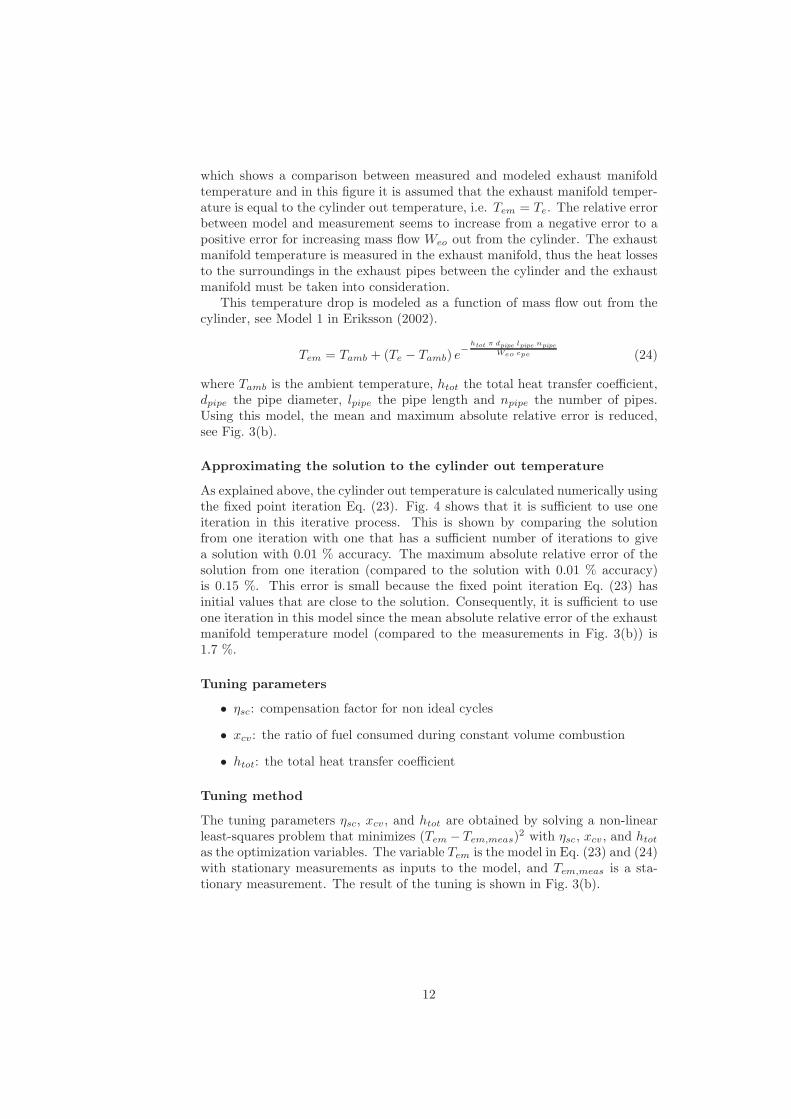
This temperature drop is modeled as a function of mass flow out from thecylinder, see Model 1 in Eriksson (2002).

Tem = Tamb + (Te − Tamb) e−

htot π dpipe lpipe npipeWeo cpe (24)

where Tamb is the ambient temperature, htot the total heat transfer coefficient,dpipe the pipe diameter, lpipe the pipe length and npipe the number of pipes.Using this model, the mean and maximum absolute relative error is reduced,see Fig. 3(b).

Approximating the solution to the cylinder out temperature

As explained above, the cylinder out temperature is calculated numerically usingthe fixed point iteration Eq. (23). Fig. 4 shows that it is sufficient to use oneiteration in this iterative process. This is shown by comparing the solutionfrom one iteration with one that has a sufficient number of iterations to givea solution with 0.01 % accuracy. The maximum absolute relative error of thesolution from one iteration (compared to the solution with 0.01 % accuracy)is 0.15 %. This error is small because the fixed point iteration Eq. (23) hasinitial values that are close to the solution. Consequently, it is sufficient to useone iteration in this model since the mean absolute relative error of the exhaustmanifold temperature model (compared to the measurements in Fig. 3(b)) is1.7 %.

Tuning parameters

• ηsc: compensation factor for non ideal cycles

• xcv: the ratio of fuel consumed during constant volume combustion

• htot: the total heat transfer coefficient

Tuning method

The tuning parameters ηsc, xcv, and htot are obtained by solving a non-linearleast-squares problem that minimizes (Tem − Tem,meas)

2 with ηsc, xcv, and htot

as the optimization variables. The variable Tem is the model in Eq. (23) and (24)with stationary measurements as inputs to the model, and Tem,meas is a sta-tionary measurement. The result of the tuning is shown in Fig. 3(b).

12

550 600 650 700 750 800 850 900500

600

700

800

900

Tem

[K]

Modeled Tem

[K]

ModeledMeasured

0.15 0.2 0.25 0.3 0.35 0.4 0.45 0.5 0.55 0.6 0.65−10

−5

0

5

10

15

rel e

rror

Tem

[%]

Weo

[kg/s]

mean abs rel error: 2.8% max abs rel error: 10.2%

(a) Without a model for heat losses in the exhaust pipes, i.e. Tem = Te.

550 600 650 700 750 800 850500

600

700

800

900

Tem

[K]

Modeled Tem

[K]

ModeledMeasured

0.15 0.2 0.25 0.3 0.35 0.4 0.45 0.5 0.55 0.6 0.65−6

−4

−2

0

2

4

6

rel e

rror

Tem

[%]

Weo

[kg/s]

mean abs rel error: 1.7% max abs rel error: 5.4%

(b) With model (24) for heat losses in the exhaust pipes.

Figure 3: Modeled and measured exhaust manifold temperature Tem and rela-tive errors for modeled Tem at steady state.

13

510 512 514 516 518 520 522 524 526 528 530200

400

600

800

1000

1200

1400

Te [K

]

One iteration0.01 % accuracy

510 512 514 516 518 520 522 524 526 528 530−0.2

−0.15

−0.1

−0.05

0

0.05

0.1

0.15

rel e

rror

[%]

Time [s]

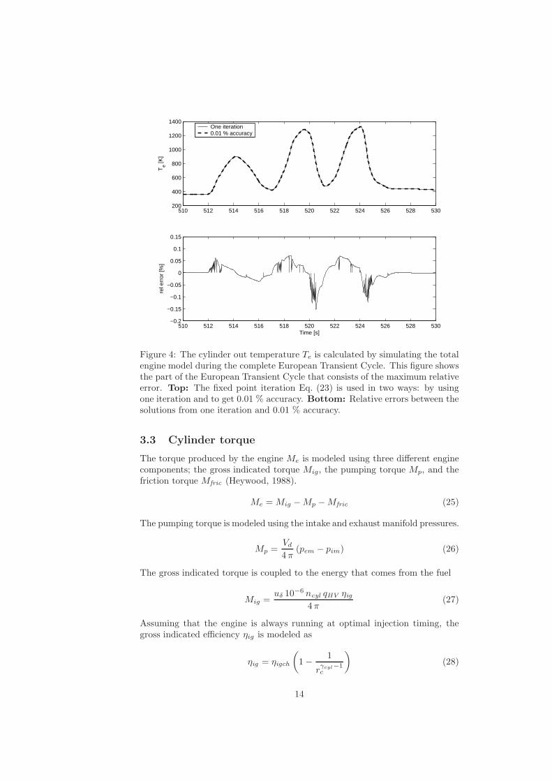
Figure 4: The cylinder out temperature Te is calculated by simulating the totalengine model during the complete European Transient Cycle. This figure showsthe part of the European Transient Cycle that consists of the maximum relativeerror. Top: The fixed point iteration Eq. (23) is used in two ways: by usingone iteration and to get 0.01 % accuracy. Bottom: Relative errors between thesolutions from one iteration and 0.01 % accuracy.

3.3 Cylinder torque

The torque produced by the engine Me is modeled using three different enginecomponents; the gross indicated torque Mig, the pumping torque Mp, and thefriction torque Mfric (Heywood, 1988).

Me = Mig −Mp −Mfric (25)

The pumping torque is modeled using the intake and exhaust manifold pressures.

Mp =Vd

4 π(pem − pim) (26)

The gross indicated torque is coupled to the energy that comes from the fuel

Mig =uδ 10

−6 ncyl qHV ηig4 π

(27)

Assuming that the engine is always running at optimal injection timing, thegross indicated efficiency ηig is modeled as

ηig = ηigch

(

1− 1

rγcyl−1c

)

(28)

14

200 400 600 800 1000 1200 1400 1600 1800 2000 22000

500

1000

1500

2000

2500M

e [Nm

]

Modeled Me [Nm]

ModeledMeasured

0.1 0.15 0.2 0.25 0.3 0.35 0.4 0.45 0.5 0.55 0.6−8

−6

−4

−2

0

2

4

rel e

rror

Me [%

]

Wc [kg/s]

mean abs rel error: 1.9% max abs rel error: 7.1%

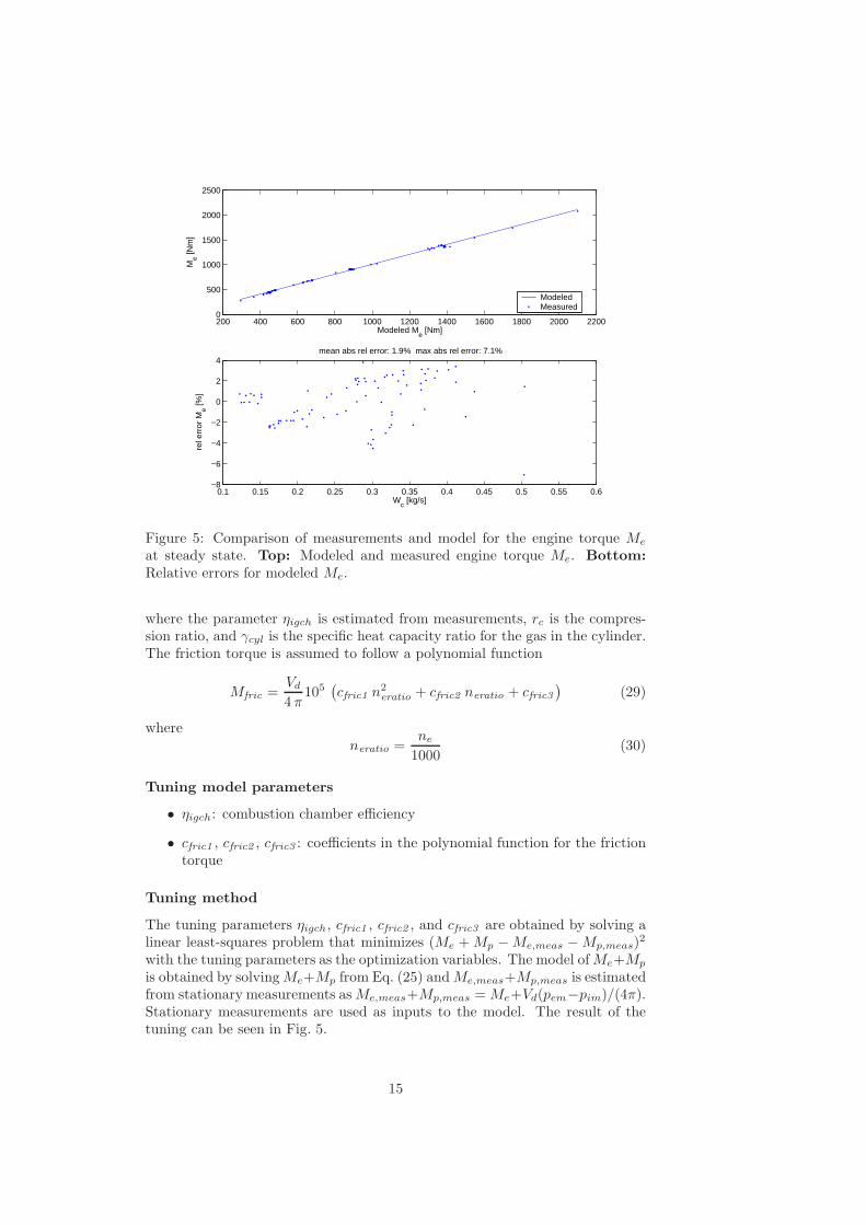
Figure 5: Comparison of measurements and model for the engine torque Me

at steady state. Top: Modeled and measured engine torque Me. Bottom:

Relative errors for modeled Me.

where the parameter ηigch is estimated from measurements, rc is the compres-sion ratio, and γcyl is the specific heat capacity ratio for the gas in the cylinder.The friction torque is assumed to follow a polynomial function

Mfric =Vd

4 π105

(

cfric1 n2eratio + cfric2 neratio + cfric3

)

(29)

whereneratio =

ne

1000(30)

Tuning model parameters

• ηigch: combustion chamber efficiency

• cfric1 , cfric2 , cfric3 : coefficients in the polynomial function for the frictiontorque

Tuning method

The tuning parameters ηigch, cfric1 , cfric2 , and cfric3 are obtained by solving alinear least-squares problem that minimizes (Me +Mp −Me,meas −Mp,meas)

2

with the tuning parameters as the optimization variables. The model ofMe+Mp

is obtained by solvingMe+Mp from Eq. (25) andMe,meas+Mp,meas is estimatedfrom stationary measurements asMe,meas+Mp,meas = Me+Vd(pem−pim)/(4π).Stationary measurements are used as inputs to the model. The result of thetuning can be seen in Fig. 5.

15

4 EGR-valve

The mass flow through the EGR-valve is modeled as a simplification of a com-pressible flow restriction with variable area (Heywood, 1988) and with the as-sumption that there is no reverse flow when pem < pim. The motive for thisassumption is to construct a simple model. The model can be extended withreverse flow, but this increases the complexity of the model since a reverse flowmodel requires mixing of different temperatures and oxygen fractions in the ex-haust manifold and a change of the temperature and the gas constant in theEGR mass flow model. However, pem is larger than pim in normal operatingpoints, consequently the assumption above will not effect the model behaviorin these operating points. Furthermore, reverse flow is not measured and cantherefore not be validated.

The mass flow through the restriction is

Wegr =Aegr pem Ψegr√

Tem Re

(31)

where

Ψegr =

√

2 γeγe − 1

(

Π2/γeegr −Π

1+1/γeegr

)

(32)

Measurement data shows that Eq. (32) does not give a sufficiently accuratedescription of the EGR flow. Pressure pulsations in the exhaust manifold orthe influence of the EGR-cooler could be two different explanations for thisphenomenon. In order to maintain the density influence (pem/(

√Tem Re)) in

Eq. (31) and the simplicity in the model, the function Ψegr is instead modeledas a parabolic function (see Fig. 6 where Ψegr is plotted as function of Πegr).

Ψegr = 1−(

1−Πegr

1−Πegropt− 1

)2

(33)

The pressure quotient Πegr over the valve is limited when the flow is choked,i.e. when sonic conditions are reached in the throat, and when 1 < pim/pem,i.e. no backflow can occur.

Πegr =

Πegropt if pim

pem< Πegropt

pim

pemif Πegropt ≤ pim

pem≤ 1

1 if 1 < pim

pem

(34)

For a compressible flow restriction, the standard model for Πegropt is

Πegropt =

(

2

γe + 1

)

γeγe−1

(35)

but the accuracy of the EGR flow model is improved by replacing the physicalvalue of Πegropt in Eq. (35) with a tuning parameter (Andersson, 2005).

The effective area

Aegr = Aegrmax fegr(uegr) (36)

16

0.7 0.75 0.8 0.85 0.9 0.95 10

0.2

0.4

0.6

0.8

1Ψ

egr

Πegr

[−]

0 10 20 30 40 50 60 70 80 90 1000

0.2

0.4

0.6

0.8

1

f egr [−

]

uegr

[%]

Figure 6: Comparison of estimated points from measurements and two sub-models for the EGR flow Wegr at steady state showing how different variablesin the sub-models depend on each other. Note that this is not a validation ofthe sub-models since the estimated points for the sub-models depend on themodel tuning. Top: Ψegr as function of pressure quotient Πegr . The estimatedpoints are calculated by solving Ψegr from Eq. (31). The model is described byEq. (33). Bottom: Effective area ratio fegr as function of control signal uegr .The estimated points are calculated by solving fegr from Eq. (31). The modelis described by Eq. (37).

is modeled as a polynomial function of the EGR valve position uegr (see Fig. 6where fegr is plotted as function of uegr)

fegr(uegr) =

cegr1 u2egr + cegr2 uegr + cegr3 if uegr ≤ − cegr2

2 cegr1

cegr3 −c2egr24 cegr1

if uegr > − cegr22 cegr1

(37)

where uegr describes the EGR actuator dynamic

d

dtuegr =

1

τegr(uegr(t− τdegr)− uegr) (38)

The EGR-valve is open when uegr = 100% and closed when uegr = 0%. Thevalues of τegr and τdegr have been provided by industry.

17

0 0.02 0.04 0.06 0.08 0.1 0.12 0.140

0.02

0.04

0.06

0.08

0.1

0.12

0.14

Weg

r [kg/

s]

Modeled Wegr

[kg/s]

ModeledCalculated from measurements

0 0.02 0.04 0.06 0.08 0.1 0.12 0.14−20

−10

0

10

20

30mean abs rel error: 6.1% max abs rel error: 22.2%

rel e

rror

Weg

r [%]

Modeled Wegr

[kg/s]

Figure 7: Top: Comparison between modeled EGR flow Wegr and estimatedWegr from measurements at steady state. Bottom: Relative errors for Wegr atsteady state.

Tuning parameters

• Πegropt: optimal value of Πegr for maximum value of the function Ψegr inEq. (33)

• cegr1, cegr2, cegr3: coefficients in the polynomial function for the effectivearea

Tuning method

The tuning parameter Πegropt is obtained by solving a non-linear least-squaresproblem that minimizes (Wegr −Wegr,meas)

2 with Πegropt as the optimizationvariable. In each iteration in the non-linear least-squares solver, the valuesfor cegr1, cegr2, and cegr3 are set to be the solution of a linear least-squaresproblem that minimizes (Wegr−Wegr,meas)

2 for the current value of Πegropt. ThevariableWegr is described by the model Eq. (31) andWegr,meas is estimated frommeasurements as Wegr,meas = Wc xegr/(1−xegr). Stationary measurements areused as inputs to the model. The result of the tuning is shown in Fig. 7.

18

5 Turbocharger

The turbocharger consist of a turbo inertia model, a turbine model, and acompressor model.

5.1 Turbo inertia

For the turbo speed ωt, Newton’s second law gives

d

dtωt =

Pt ηm − Pc

Jt ωt(39)

where Jt is the inertia, Pt is the power delivered by the turbine, Pc is the powerrequired to drive the compressor, and ηm is the mechanical efficiency in theturbocharger.

Tuning parameter

• Jt: turbo inertia

Tuning method

The tuning parameter Jt is obtained by adjusting this parameter manually untilsimulations of the complete model follow the dynamic responses in the dynamicmeasurements, see Sec. 8.1.

5.2 Turbine

The turbine models are the total turbine efficiency and the turbine mass flow.

5.2.1 Turbine efficiency

One way to model the power Pt is to use the turbine efficiency ηt, which isdefined as (Heywood, 1988)

ηt =Pt

Pt,s=

Tem − Tt

Tem(1−Π1−1/γe

t )(40)

where Tt is the temperature after the turbine, Πt is the pressure ratio

Πt =pamb

pem(41)

and Pt,s is the power from the isentropic process

Pt,s = Wt cpe Tem

(

1−Π1−1/γe

t

)

(42)

where Wt is the turbine mass flow.However, Eq. (40) is not applicable due to heat losses in the turbine which

cause temperature drops in the temperatures Tt and Tem. Consequently, therewill be errors for ηt if Eq. (40) is used to calculate ηt from measurements. Oneway to overcome this is to model the temperature drops, but it is difficult to tunethese models since there exists no measurements of these temperature drops.

19

Another way to overcome this, that is frequently used in the literature, is touse another efficiency that are approximatively equal to ηt. This approximationutilizes that

Pt ηm = Pc (43)

at steady state according to Eq. (39). Consequently, Pt ≈ Pc at steady state.Using this approximation in Eq. (40), another efficiency ηtm is obtained

ηtm =Pc

Pt,s=

Wc cpa(Tc − Tamb)

Wt cpe Tem

(

1−Π1−1/γe

t

) (44)

where Tc is the temperature after the compressor and Wc is the compressor massflow. The temperature Tem in Eq. (44) introduces less errors compared to thetemperature difference Tem−Tt in Eq. (40) due to that the absolute value of Tem

is larger than the absolute value of Tem−Tt. Consequently, Eq. (44) introducesless errors compared to Eq. (40) since Eq. (44) does not consist of Tem − Tt.The temperatures Tc and Tamb are low and they introduce less errors comparedto Tem and Tt since the heat losses in the compressor are comparatively small.Another advantage of using Eq. (44) is that the individual variables Pt and ηmin Eq. (39) do not have to be modeled. Instead, the product Pt ηm is modeledusing Eq. (43) and (44)

Pt ηm = Pc = ηtm Pt,s = ηtm Wt cpe Tem

(

1−Π1−1/γe

t

)

(45)

Measurements show that ηtm depends on the blade speed ratio (BSR) as aparabolic function (Watson and Janota, 1982), see Fig. 8 where ηtm is plottedas function of BSR.

ηtm = ηtm,max − cm(BSR−BSRopt)2 (46)

The blade speed ratio is the quotient of the turbine blade tip speed and thespeed which a gas reaches when expanded isentropically at the given pressureratio Πt

BSR =Rt ωt

√

2 cpe Tem

(

1−Π1−1/γe

t

)

(47)

whereRt is the turbine blade radius. The parameter cm in the parabolic functionvaries due to mechanical losses and cm is therefore modeled as a function of theturbo speed

cm = cm1(ωt − cm2)cm3 (48)

see Fig. 8 where cm is plotted as function of ωt.

Tuning parameters

• ηtm,max: maximum turbine efficiency

• BSRopt: optimum BSR value for maximum turbine efficiency

• cm1, cm2, cm3: parameters in the model for cm

20

0.52 0.54 0.56 0.58 0.6 0.62 0.640.4

0.5

0.6

0.7

0.8

0.9

2680

10640

η tm [−

]

BSR [−]

2000 3000 4000 5000 6000 7000 8000 9000 10000 11000−0.5

0

0.5

1

1.5

2

2.5

c m [−

]

ωt [rad/s]

Figure 8: Comparison of estimated points from measurements and the modelfor the turbine efficiency ηtm at steady state. Top: ηtm as function of bladespeed ratio BSR. The estimated points are calculated by using Eq. (44) and(47). The model Eq. (46) is plotted at two different turbo speeds ωt. Bottom:

Parameter cm as function of turbo speed ωt. The estimated points are calculatedby solving cm from Eq. (46). The model is described by Eq. (48). Note thatthis plot is not a validation of cm since the estimated points for cm depend onthe model tuning.

Tuning method

The tuning parameters BSRopt, cm2, and cm3 are obtained by solving a non-linear least-squares problem that minimizes (ηtm − ηtm,meas)

2 with BSRopt,cm2, and cm3 as the optimization variables. In each iteration in the non-linearleast-squares solver, the values for ηtm,max and cm1 are set to be the solution ofa linear least-squares problem that minimizes (ηtm − ηtm,meas)

2 for the currentvalues of BSRopt, cm2, and cm3. The efficiency ηtm is described by the modelEq. (46) and ηtm,meas is estimated from measurements using Eq. (44). Station-ary measurements are used as inputs to the model. The result of the tuning isshown in Fig. 8 and 9.

5.2.2 Turbine mass flow

The turbine mass flow Wt is modeled using the corrected mass flow (Heywood,1988; Watson and Janota, 1982)

Wt

√Tem

pem= Avgtmax fΠt(Πt) fvgt(uvgt) (49)

21

1 1.5 2 2.5 3 3.5 4

x 105

−15

−10

−5

0

5

10

15

rel e

rror

ηtm

[%]

pem

[Pa]

mean abs rel error: 4.2% max abs rel error: 13.2%

Figure 9: Relative errors for the total turbine efficiency ηtm as function ofexhaust manifold pressure pem at steady state.

where Avgtmax is the maximum area in the turbine that the gas flows through.Measurements show that the corrected mass flow depends on the pressure ratioΠt and the VGT actuator signal uvgt. As the pressure ratio decreases, thecorrected mass flow increases until the gas reaches the sonic condition and theflow is choked. This behavior can be described by a choking function

fΠt(Πt) =

√

1−ΠKt

t (50)

which is not based on the physics of the turbine, but it gives good agreementwith measurements using few parameters (Eriksson et al., 2002), see Fig. 10where fΠt is plotted as function of Πt.

When the VGT control signal uvgt increases, the effective area increases andhence also the flow increases. Due to the geometry in the turbine, the change ineffective area is large when the VGT control signal is large. This behavior canbe described by a part of an ellipse (see Fig. 10 where fvgt is plotted as functionof uvgt)

(

fvgt(uvgt)− cf2cf1

)2

+

(

uvgt − cvgt2cvgt1

)2

= 1 (51)

where fvgt is the effective area ratio function and uvgt describes the VGT actu-ator dynamic

d

dtuvgt =

1

τvgt(uvgt − uvgt) (52)

The value of τvgt has been provided by industry. The flow can now be modeledby solving Wt from Eq. (49)

Wt =Avgtmax pem fΠt(Πt) fvgt(uvgt)√

Tem

(53)

and solving fvgt from Eq. (51)

fvgt(uvgt) = cf2 + cf1

√

1−(

uvgt − cvgt2cvgt1

)2

(54)

22

0.2 0.3 0.4 0.5 0.6 0.7 0.8 0.9 1

0.6

0.8

1

1.2

f Πt [−

]

Πt [−]

20 30 40 50 60 70 80 90 100 1100.4

0.6

0.8

1

1.2

1.4

f vgt [−

]

uvgt

[%]

Figure 10: Comparison of estimated points from measurements and two sub-models for the turbine mass flow at steady state showing how different variablesin the sub-models depend on each other. Note that this is not a validation ofthe sub-models since the estimated points for the sub-models depend on themodel tuning. Top: The choking function fΠt as function of the pressure ratioΠt. The estimated points are calculated by solving fΠt from Eq. (49). Themodel is described by Eq. (50). Bottom: The effective area ratio function fvgtas function of the control signal uvgt. The estimated points are calculated bysolving fvgt from Eq. (49). The model is described by Eq. (54).

Tuning parameters

• Kt: exponent in the choking function for the turbine flow

• cf1 , cf2 , cvgt1, cvgt2: parameters in the ellipse for the effective area ratiofunction

Tuning method

The tuning parameters above are obtained by solving a non-linear least-squaresproblem that minimizes (Wt − Wt,meas)

2 with the tuning parameters as theoptimization variables. The flow Wt is described by the model Eq. (53), (54),and (50), and Wt,meas is estimated from measurements as Wt,meas = Wc +Wf ,where Wf is estimated using Eq. (12). Stationary measurements are used asinputs to the model. The result of the tuning is shown in Fig. 11.

5.3 Compressor

The compressor models the compressor efficiency and the compressor mass flow.

23

20 30 40 50 60 70 80 90 100 110−6

−4

−2

0

2

4

6

8

rel e

rror

Wt [%

]

uvgt

[%]

mean abs rel error: 2.8% max abs rel error: 7.6%

Figure 11: Relative errors for turbine flow Wt as function of control signal uvgt

at steady state.

5.3.1 Compressor efficiency

The compressor power Pc is modeled using the compressor efficiency ηc, whichis defined as (Heywood, 1988)

ηc =Pc,s

Pc=

Tamb

(

Π1−1/γac − 1

)

Tc − Tamb(55)

where Tc is the temperature after the compressor, Πc is the pressure ratio

Πc =pimpamb

(56)

and Pc,s is the power from the isentropic process

Pc,s = Wc cpa Tamb

(

Π1−1/γac − 1

)

(57)

where Wc is the compressor mass flow. The power Pc is modeled by solving Pc

from Eq. (55) and using Eq. (57)

Pc =Pc,s

ηc=

Wc cpa Tamb

ηc

(

Π1−1/γac − 1

)

(58)

The efficiency is modeled using ellipses similar to Guzzella and Amstutz(1998), but with a non-linear transformation on the axis for the pressure ratio.The inputs to the efficiency model are Πc and Wc (see Fig. 16). The flow Wc

is not scaled by the inlet temperature and the inlet pressure since these twovariables are constant. The ellipses can be described as

ηc = ηcmax − χT Qc χ (59)

χ is a vector which contains the inputs

χ =

[

Wc −Wcopt

πc − πcopt

]

(60)

where the non-linear transformation for Πc is

πc = (Πc − 1)powπ (61)

24

0.1 0.15 0.2 0.25 0.3 0.35 0.4 0.45 0.5 0.55 0.6−15

−10

−5

0

5

10

15mean abs rel error: 3.3% max abs rel error: 14.1%

rel e

rror

ηc [%

]

Wc [kg/s]

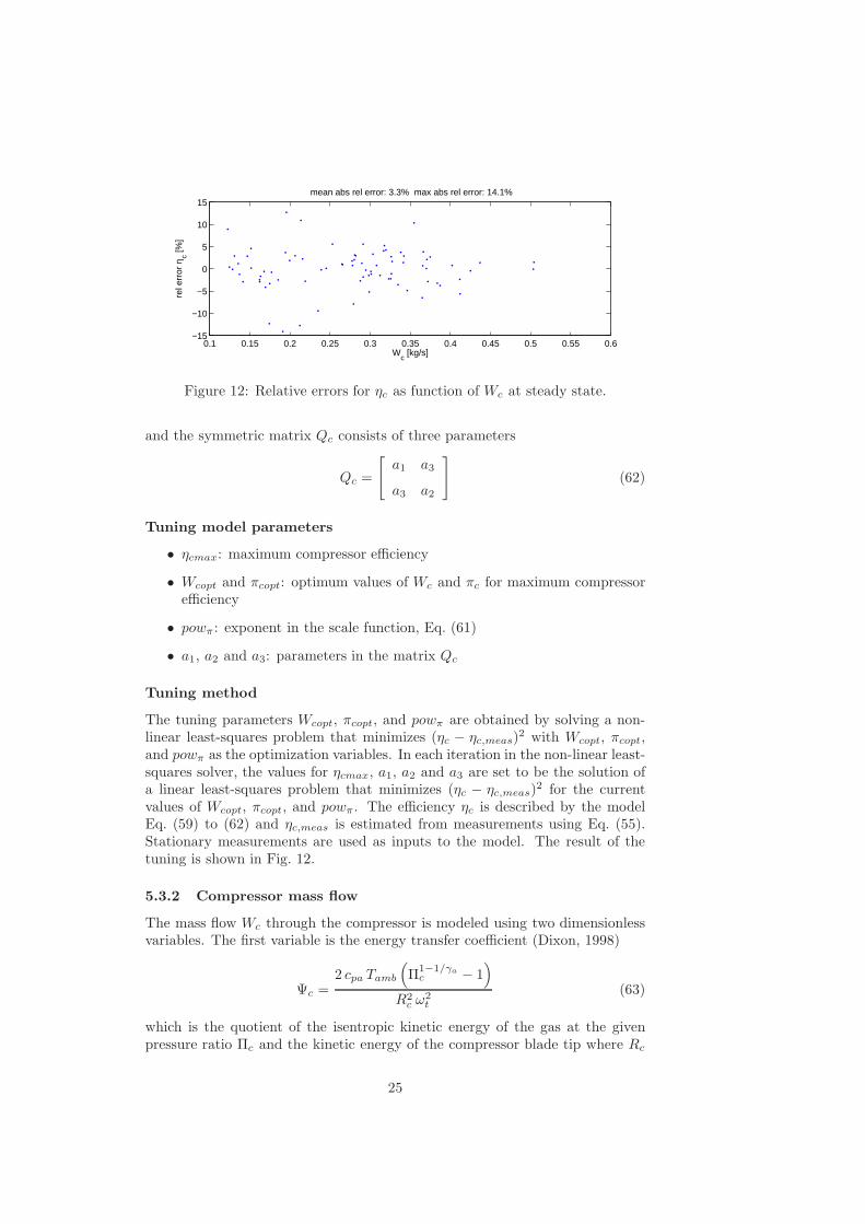
Figure 12: Relative errors for ηc as function of Wc at steady state.

and the symmetric matrix Qc consists of three parameters

Qc =

[

a1 a3

a3 a2

]

(62)

Tuning model parameters

• ηcmax: maximum compressor efficiency

• Wcopt and πcopt: optimum values of Wc and πc for maximum compressorefficiency

• powπ : exponent in the scale function, Eq. (61)

• a1, a2 and a3: parameters in the matrix Qc

Tuning method

The tuning parameters Wcopt, πcopt, and powπ are obtained by solving a non-linear least-squares problem that minimizes (ηc − ηc,meas)

2 with Wcopt, πcopt,and powπ as the optimization variables. In each iteration in the non-linear least-squares solver, the values for ηcmax, a1, a2 and a3 are set to be the solution ofa linear least-squares problem that minimizes (ηc − ηc,meas)

2 for the currentvalues of Wcopt, πcopt, and powπ. The efficiency ηc is described by the modelEq. (59) to (62) and ηc,meas is estimated from measurements using Eq. (55).Stationary measurements are used as inputs to the model. The result of thetuning is shown in Fig. 12.

5.3.2 Compressor mass flow

The mass flow Wc through the compressor is modeled using two dimensionlessvariables. The first variable is the energy transfer coefficient (Dixon, 1998)

Ψc =2 cpa Tamb

(

Π1−1/γac − 1

)

R2c ω

2t

(63)

which is the quotient of the isentropic kinetic energy of the gas at the givenpressure ratio Πc and the kinetic energy of the compressor blade tip where Rc

25

0.2 0.4 0.6 0.8 1 1.2 1.4 1.60

0.1

0.2

0.3

0.4

270053008000

10600

Ψc [−]

Φc [−

]

Figure 13: Comparison of estimated points from measurements and model forthe compressor mass flow Wc at steady state. Volumetric flow coefficient Φc asfunction of energy transfer coefficient Ψc. The estimated points are calculatedusing Eq. (63) and (64). The model (Eq. 68) is plotted at four different turbospeeds ωt.

is compressor blade radius. The second variable is the volumetric flow coeffi-cient (Dixon, 1998)

Φc =Wc/ρamb

π R3c ωt

=Ra Tamb

pamb π R3c ωt

Wc (64)

which is the quotient of volume flow rate of air into the compressor and the rateat which volume is displaced by the compressor blade where ρamb is the densityof the ambient air. The relation between Ψc and Φc can be described by a partof an ellipse (Andersson, 2005), see Fig. 13 where Φc is plotted as function ofΨc.

cΨ1(ωt) (Ψc − cΨ2)2+ cΦ1(ωt) (Φc − cΦ2)

2= 1 (65)

where cΨ1 and cΦ1 varies with turbo speed ωt and are modeled as polynomialfunctions.

cΨ1(ωt) = cωΨ1 ω2t + cωΨ2 ωt + cωΨ3 (66)

cΦ1(ωt) = cωΦ1 ω2t + cωΦ2 ωt + cωΦ3 (67)

In Fig. 14 the variables cΨ1 and cΦ1 are plotted as function of the turbo speedωt.

The mass flow is modeled by solving Φc from Eq. (65) and solving Wc fromEq. (64).

Φc =

√

1− cΨ1 (Ψc − cΨ2)2

cΦ1

+ cΦ2 (68)

Wc =pamb π R3

c ωt

Ra TambΦc (69)

Tuning model parameters

• cΨ2, cΦ2: parameters in the ellipse model for the compressor mass flow

• cωΨ1, cωΨ2, cωΨ3: coefficients in the polynomial function Eq. (66)

• cωΦ1, cωΦ2, cωΦ3: coefficients in the polynomial function Eq. (67)

26

2000 3000 4000 5000 6000 7000 8000 9000 10000 110000.3

0.4

0.5

0.6

0.7

c Ψ1 [−

]

ωt [rad/s]

2000 3000 4000 5000 6000 7000 8000 9000 10000 1100010

15

20

25

30

c Φ1 [−

]

ωt [rad/s]

Figure 14: Comparison of estimated points from measurements and two sub-models for the compressor mass flow at steady state showing how different vari-ables in the sub-models depend on each other. Note that this is not a validationof the sub-models since the estimated points for the sub-models depend on themodel tuning. The sub-models are the ellipse variables cΨ1 and cΦ1 as functionof turbo speed ωt. The estimated points are calculated by solving cΨ1 and cΦ1

from Eq. (65). The models are described by Eq. (66) and (67).

Tuning method

The tuning parameters cΨ2 and cΦ2 are obtained by solving a non-linear least-squares problem that minimizes (cΨ1(ωt) (Ψc − cΨ2)

2+cΦ1(ωt) (Φc − cΦ2)2−1)2

with cΨ2 and cΦ2 as the optimization variables. In each iteration in the non-linear least-squares solver, the values for cωΨ1, cωΨ2, cωΨ3, cωΦ1, cωΦ2, andcωΦ3 are set to be the solution of a linear least-squares problem that minimizes(cΨ1(ωt) (Ψc − cΨ2)

2+ cΦ1(ωt) (Φc − cΦ2)

2 − 1)2 for the current values of cΨ2

and cΦ2. Stationary measurements are used as inputs to the model. The resultof the tuning is shown in Fig. 15.

5.3.3 Compressor map

Compressor performance is usually presented by a map with constant efficiencylines and constant turbo speed lines and with Πc and Wc on the axes. This isshown in Fig. 16 which has approximatively the same characteristics as Fig. 2.10in Watson and Janota (1982). Consequently, the proposed compressor modelhas the expected behavior.

27

2000 3000 4000 5000 6000 7000 8000 9000 10000 11000−15

−10

−5

0

5

10

rel e

rror

Wc [%

]

ωt [rad/s]

mean abs rel error: 3.4% max abs rel error: 13.7%

Figure 15: Relative errors for compressor flow Wc as function of turbochargerspeed ωt at steady state.

0 0.1 0.2 0.3 0.4 0.5 0.6 0.71

1.5

2

2.5

3

3.5

4

Wc [kg/s]

Πc [−

]

0.5

0.5

0.5

0.5

0.5

0.5

0.55

0.55

0.55

0.55

0.55

0.55

0.6

0.6

0.6

0.6

0.6

0.6

0.6

0.65

0.65

0.65

0.65

0.65

0.65

0.65

0.7

0.7

0.7

0.7

0.7

0.7

0.7

0.73

0.73

0.73

0.73

40005000

6000

7000

8000

9000

10000

11000

12000

ηc < 0.5

0.5 < ηc < 0.55

0.55 < ηc < 0.6

0.6 < ηc < 0.65

0.65 < ηc < 0.7

0.7 < ηc < 0.73

0.73 < ηc

Figure 16: Compressor map with modeled efficiency lines (solid line), modeledturbo speed lines (dashed line with turbo speed in rad/s), and estimated ef-ficiency from measurements using Eq. (55). The estimated points are dividedinto different groups. The turbo speed lines are described by the compressorflow model.

28

6 Intercooler and EGR-cooler

To construct a simple model, that captures the important system properties,the intercooler and the EGR-cooler are assumed to be ideal, i.e. the equationsfor the coolers are

pout = pin

Wout = Win

Tout = Tcool

(70)

where Tcool is the cooling temperature. The model can be extended with non-ideal coolers, but these increase the complexity of the model since non-idealcoolers require that there are states for the pressures both before and after thecoolers.

29

7 Summary of assumptions and model equations

A summary of the model assumptions is given in Sec. 7.1 and the proposedmodel equations are given in Sec. 7.2 to 7.5.

7.1 Assumptions

To develop a simple model, that captures the dominating effects in the massflows, the following assumptions are made:

• The intercooler and the EGR-cooler are ideal, i.e. the equations for thecoolers are

pout = pin

Wout = Win

Tout = Tcool

(71)

where Tcool is the cooling temperature.

• The manifolds are modeled as standard isothermal models.

• All gases are considered to be ideal and there are two sets of thermody-namic properties:

1. Air has the gas constant Ra and the specific heat capacity ratio γa.

2. Exhaust gas has the gas constant Re and the specific heat capacityratio γe.

• No heat transfer to or from the gas inside of the intake manifold.

• No backflow can occur.

• The intake manifold temperature is constant.

• The oxygen fuel ratio λO is always larger than one.

7.2 Manifolds

d

dtpim =

Ra Tim

Vim(Wc +Wegr −Wei)

d

dtpem =

Re Tem

Vem

(Weo −Wt −Wegr)

(72)

xegr =Wegr

Wc +Wegr(73)

d

dtXOim =

Ra Tim

pim Vim((XOem −XOim)Wegr + (XOc −XOim)Wc)

d

dtXOem =

Re Tem

pem Vem

(XOe −XOem) Weo

(74)

30

7.3 Cylinder

7.3.1 Cylinder flow

Wei =ηvol pim ne Vd

120Ra Tim(75)

ηvol = cvol1√pim + cvol2

√ne + cvol3 (76)

Wf =10−6

120uδ ne ncyl (77)

Weo = Wf +Wei (78)

λO =Wei XOim

Wf (O/F )s(79)

XOe =Wei XOim −Wf (O/F )s

Weo(80)

7.3.2 Cylinder out temperature

qin,k+1 =Wf qHV

Wei +Wf

(1− xr,k)

xp,k+1 = 1 +qin,k+1 xcv

cva T1,k rγa−1c

xv,k+1 = 1 +qin,k+1 (1− xcv )

cpa

(

qin,k+1 xcv

cva+ T1,k r

γa−1c

)

xr,k+1 =Π

1/γae x

−1/γa

p,k+1

rc xv,k+1

Te,k+1 = ηsc Π1−1/γae r1−γa

c x1/γa−1

p,k+1

(

qin,k+1

(

1− xcv

cpa+

xcv

cva

)

+ T1,k rγa−1c

)

T1,k+1 = xr,k+1 Te,k+1 + (1− xr,k+1)Tim

(81)

Tem = Tamb + (Te − Tamb) e−

htot π dpipe lpipe npipeWeo cpe (82)

7.3.3 Cylinder torque

Me = Mig −Mp −Mfric (83)

Mp =Vd

4 π(pem − pim) (84)

Mig =uδ 10

−6 ncyl qHV ηig4 π

(85)

ηig = ηigch

(

1− 1

rγcyl−1c

)

(86)

Mfric =Vd

4 π105

(

cfric1 n2eratio + cfric2 neratio + cfric3

)

(87)

neratio =ne

1000(88)

31

7.4 EGR-valve

Wegr =Aegr pem Ψegr√

Tem Re

(89)

Ψegr = 1−(

1−Πegr

1−Πegropt− 1

)2

(90)

Πegr =

Πegropt if pim

pem< Πegropt

pim

pemif Πegropt ≤ pim

pem≤ 1

1 if 1 < pim

pem

(91)

Aegr = Aegrmax fegr(uegr) (92)

fegr(uegr) =

cegr1 u2egr + cegr2 uegr + cegr3 if uegr ≤ − cegr2

2 cegr1

cegr3 − c2egr24 cegr1

if uegr > − cegr22 cegr1

(93)

d

dtuegr =

1

τegr(uegr(t− τdegr)− uegr) (94)

7.5 Turbo

7.5.1 Turbo inertia

d

dtωt =

Pt ηm − Pc

Jt ωt(95)

7.5.2 Turbine efficiency

Pt ηm = ηtm Wt cpe Tem

(

1−Π1−1/γe

t

)

(96)

Πt =pamb

pem(97)

ηtm = ηtm,max − cm(BSR−BSRopt)2 (98)

BSR =Rt ωt

√

2 cpe Tem

(

1−Π1−1/γe

t

)

(99)

cm = cm1(ωt − cm2)cm3 (100)

32

7.5.3 Turbine mass flow

Wt =Avgtmax pem fΠt(Πt) fvgt(uvgt)√

Tem

(101)

fΠt(Πt) =

√

1−ΠKt

t (102)

fvgt(uvgt) = cf2 + cf1

√

1−(

uvgt − cvgt2cvgt1

)2

(103)

d

dtuvgt =

1

τvgt(uvgt − uvgt) (104)

7.5.4 Compressor efficiency

Pc =Wc cpa Tamb

ηc

(

Π1−1/γac − 1

)

(105)

Πc =pimpamb

(106)

ηc = ηcmax − χT Qc χ (107)

χ =

[

Wc −Wcopt

πc − πcopt

]

(108)

πc = (Πc − 1)powπ (109)

Qc =

[

a1 a3

a3 a2

]

(110)

7.5.5 Compressor mass flow

Wc =pamb π R3

c ωt

Ra TambΦc (111)

Φc =

√

1− cΨ1 (Ψc − cΨ2)2

cΦ1

+ cΦ2 (112)

Ψc =2 cpa Tamb

(

Π1−1/γac − 1

)

R2c ω

2t

(113)

cΨ1 = cωΨ1 ω2t + cωΨ2 ωt + cωΨ3 (114)

cΦ1 = cωΦ1 ω2t + cωΦ2 ωt + cωΦ3 (115)

33

8 Model tuning and validation

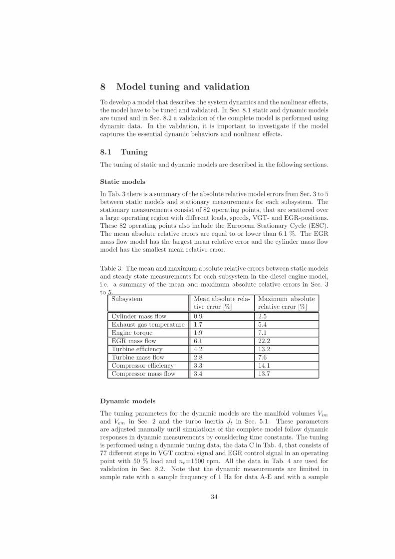
To develop a model that describes the system dynamics and the nonlinear effects,the model have to be tuned and validated. In Sec. 8.1 static and dynamic modelsare tuned and in Sec. 8.2 a validation of the complete model is performed usingdynamic data. In the validation, it is important to investigate if the modelcaptures the essential dynamic behaviors and nonlinear effects.

8.1 Tuning

The tuning of static and dynamic models are described in the following sections.

Static models

In Tab. 3 there is a summary of the absolute relative model errors from Sec. 3 to 5between static models and stationary measurements for each subsystem. Thestationary measurements consist of 82 operating points, that are scattered overa large operating region with different loads, speeds, VGT- and EGR-positions.These 82 operating points also include the European Stationary Cycle (ESC).The mean absolute relative errors are equal to or lower than 6.1 %. The EGRmass flow model has the largest mean relative error and the cylinder mass flowmodel has the smallest mean relative error.

Table 3: The mean and maximum absolute relative errors between static modelsand steady state measurements for each subsystem in the diesel engine model,i.e. a summary of the mean and maximum absolute relative errors in Sec. 3to 5.

Subsystem Mean absolute rela-tive error [%]

Maximum absoluterelative error [%]

Cylinder mass flow 0.9 2.5Exhaust gas temperature 1.7 5.4Engine torque 1.9 7.1EGR mass flow 6.1 22.2Turbine efficiency 4.2 13.2Turbine mass flow 2.8 7.6Compressor efficiency 3.3 14.1Compressor mass flow 3.4 13.7

Dynamic models

The tuning parameters for the dynamic models are the manifold volumes Vim

and Vem in Sec. 2 and the turbo inertia Jt in Sec. 5.1. These parametersare adjusted manually until simulations of the complete model follow dynamicresponses in dynamic measurements by considering time constants. The tuningis performed using a dynamic tuning data, the data C in Tab. 4, that consists of77 different steps in VGT control signal and EGR control signal in an operatingpoint with 50 % load and ne=1500 rpm. All the data in Tab. 4 are used forvalidation in Sec. 8.2. Note that the dynamic measurements are limited insample rate with a sample frequency of 1 Hz for data A-E and with a sample

34

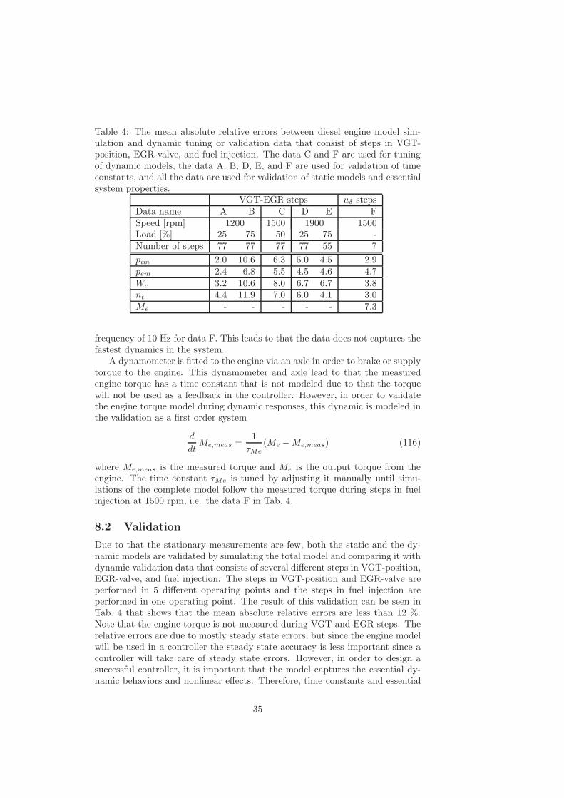
Table 4: The mean absolute relative errors between diesel engine model sim-ulation and dynamic tuning or validation data that consist of steps in VGT-position, EGR-valve, and fuel injection. The data C and F are used for tuningof dynamic models, the data A, B, D, E, and F are used for validation of timeconstants, and all the data are used for validation of static models and essentialsystem properties.

VGT-EGR steps uδ stepsData name A B C D E FSpeed [rpm] 1200 1500 1900 1500Load [%] 25 75 50 25 75 -Number of steps 77 77 77 77 55 7

pim 2.0 10.6 6.3 5.0 4.5 2.9pem 2.4 6.8 5.5 4.5 4.6 4.7Wc 3.2 10.6 8.0 6.7 6.7 3.8nt 4.4 11.9 7.0 6.0 4.1 3.0Me - - - - - 7.3

frequency of 10 Hz for data F. This leads to that the data does not captures thefastest dynamics in the system.

A dynamometer is fitted to the engine via an axle in order to brake or supplytorque to the engine. This dynamometer and axle lead to that the measuredengine torque has a time constant that is not modeled due to that the torquewill not be used as a feedback in the controller. However, in order to validatethe engine torque model during dynamic responses, this dynamic is modeled inthe validation as a first order system

d

dtMe,meas =

1

τMe(Me −Me,meas) (116)

where Me,meas is the measured torque and Me is the output torque from theengine. The time constant τMe is tuned by adjusting it manually until simu-lations of the complete model follow the measured torque during steps in fuelinjection at 1500 rpm, i.e. the data F in Tab. 4.

8.2 Validation

Due to that the stationary measurements are few, both the static and the dy-namic models are validated by simulating the total model and comparing it withdynamic validation data that consists of several different steps in VGT-position,EGR-valve, and fuel injection. The steps in VGT-position and EGR-valve areperformed in 5 different operating points and the steps in fuel injection areperformed in one operating point. The result of this validation can be seen inTab. 4 that shows that the mean absolute relative errors are less than 12 %.Note that the engine torque is not measured during VGT and EGR steps. Therelative errors are due to mostly steady state errors, but since the engine modelwill be used in a controller the steady state accuracy is less important since acontroller will take care of steady state errors. However, in order to design asuccessful controller, it is important that the model captures the essential dy-namic behaviors and nonlinear effects. Therefore, time constants and essential

35

system properties are validated in the following sections.

Validation of time constants

In Sec. 8.1, the dynamic models are tuned by considering the time constants inthe data C in Tab. 4. These time constants are validated using the dynamicvalidation data A, B, D, and E in Tab. 4. Some parts of this validation areplotted in Fig. 17 and 18. The non-minimum phase behavior in pim in Fig. 17shows that the model captures the fast dynamic in the beginning of the responseand that the model captures the slow dynamic in the end of the response. Theovershoot in the third response in Fig. 18 also shows that model captures bothfast and slow dynamics.

Validation of essential system properties

Kolmanovsky et al. (1997) and Jung (2003) show the essential system propertiesfor the pressures and the flows in a diesel engine with VGT and EGR. Someof these properties are a non-minimum phase behavior in the intake manifoldpressure and a non-minimum phase behavior, an overshoot, and a sign reversalin the compressor mass flow. These system properties are validated using thedynamic data A-E in Tab. 4. Some parts of this validation are shown in Fig. 17to 19. Fig. 17 shows that the model captures the non-minimum phase behaviorin the transfer function uegr to pim and the second step in Fig. 19 shows thatthe model captures the non-minimum phase behavior in the transfer functionuvgt to Wc. Note that the non-minimum phase behaviors in the measurementsare not obvious due to a low sample frequency. Further, the third step in Fig. 18and the third step in Fig. 19 show that the model captures the overshoot andthe sign reversal in the transfer function uvgt to Wc.

36

0 5 10 15 200

20

40

60u eg

r [%]

0 5 10 15 201.5

1.6

1.7

1.8

1.9x 10

5

Time [s]

p im [P

a]

simmeas

Figure 17: Comparison between diesel engine model simulation and dynamicvalidation data during steps in EGR-valve position showing that the modelcaptures the non-minimum phase behavior in pim. Operating point: 25 % load,ne=1900 rpm and uvgt=50 %.

0 5 10 15 20 25 30 35 4020

40

60

80

100

u vgt [%

]

0 5 10 15 20 25 30 35 400.15

0.2

0.25

0.3

0.35

Time [s]

Wc [k

g/s]

simmeas

Figure 18: Comparison between diesel engine model simulation and dynamic val-idation data during steps in VGT position showing that the model captures theovershoot and the sign reversal inWc. Operating point: 75 % load, ne=1200 rpmand uegr=40 %.

37

0 5 10 15 20 25 3020

40

60

80

100

u vgt [%

]

0 5 10 15 20 25 300.2

0.25

0.3

0.35

Time [s]

Wc [k

g/s]

simmeas

Figure 19: Comparison between diesel engine model simulation and dynamictuning data during steps in VGT position showing that the model capturesthe non-minimum phase behavior, the overshoot, and the sign reversal in Wc.Operating point: 50 % load, ne=1500 rpm and uegr=81.5 %.

38

9 Conclusions

A mean value model of a diesel engine with VGT and EGR including oxygenmass fraction was developed and validated. The intended applications of themodel are system analysis, simulation, and development of model-based con-trol systems. To be able to implement a model-based controller, the modelmust be small. Therefore the model has only seven states: intake and exhaustmanifold pressures, oxygen mass fraction in the intake and exhaust manifold,turbocharger speed, and two states describing the actuator dynamics for theEGR-valve and the VGT-position.

Model equations and tuning methods for the model parameters was de-scribed for each subsystem in the model. Parameters in the static models aretuned automatically using least square optimization and stationary measure-ments in 82 different operating points. The tuning shows that the mean relativeerrors are equal to or lower than 6.1 %. Parameters in dynamic models aretuned by adjusting these parameters manually until simulations of the completemodel follow the dynamic responses in the dynamic measurements. In order todecrease the amount of tuning parameters, flows and efficiencies are modeledusing physical relationships and parametric models instead of look-up tables.

Static and dynamic validations of the entire model were performed usingdynamic measurements, which consist of steps in fuel injection, EGR controlsignal, and VGT control signal. The validations show mean relative errorswhich are less than 12 %. The validations also show that the proposed modelcaptures the essential system properties, i.e. a non-minimum phase behaviorin the transfer function uegr to pim and a non-minimum phase behavior, anovershoot, and a sign reversal in the transfer function uvgt to Wc.

39

40

References

Andersson, P. (2005). Air Charge Estimation in Turbocharged Spark Ignition

Engines. PhD thesis, Linkopings Universitet.

Dixon, S. (1998). Fluid Mechanics and Thermodynamics of Turbomachinery.Butterworth Heinemann, Woburn, 4:th edition.

Eriksson, L. (2002). Mean value models for exhaust system temperatures. SAE2002 Transactions, Journal of Engines, 2002-01-0374, 111(3).

Eriksson, L., Nielsen, L., Brugard, J., Bergstrom, J., Pettersson, F., and An-dersson, P. (2002). Modeling and simulation of a turbo charged SI engine.Annual Reviews in Control, 26(1):129–137.

Guzzella, L. and Amstutz, A. (1998). Control of diesel engines. IEEE Control

Systems Magazine, 18:53–71.

Heywood, J. (1988). Internal Combustion Engine Fundamentals. McGraw-HillBook Co.

Jung, M. (2003). Mean-Value Modelling and Robust Control of the Airpath of

a Turbocharged Diesel Engine. PhD thesis, University of Cambridge.

Kolmanovsky, I., Stefanopoulou, A., Moraal, P., and van Nieuwstadt, M.(1997). Issues in modeling and control of intake flow in variable geometryturbocharged engines. In Proceedings of 18th IFIP Conference on System

Modeling and Optimization, Detroit.

Skogtjarn, P. (2002). Modelling of the exhaust gas temperature for diesel en-gines. Master’s thesis LiTH-ISY-EX-3379, Department of Electrical Engi-neering, Linkoping University, Linkoping, Sweden.

Vigild, C. (2001). The Internal Combustion Engine Modelling, Estimation and

Control Issues. PhD thesis, Technical University of Denmark, Lyngby.

Watson, N. and Janota, M. (1982). Turbocharging the Internal Combustion

Engine. The Mechanical Press Ltd, Hong Kong.

41

42

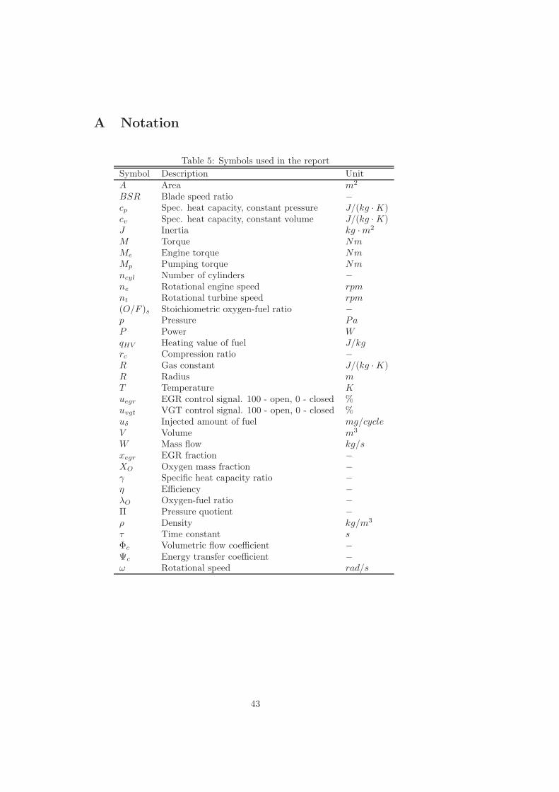
A Notation

Table 5: Symbols used in the report

Symbol Description UnitA Area m2

BSR Blade speed ratio −cp Spec. heat capacity, constant pressure J/(kg ·K)cv Spec. heat capacity, constant volume J/(kg ·K)J Inertia kg ·m2

M Torque NmMe Engine torque NmMp Pumping torque Nmncyl Number of cylinders −ne Rotational engine speed rpmnt Rotational turbine speed rpm(O/F )s Stoichiometric oxygen-fuel ratio −p Pressure PaP Power WqHV Heating value of fuel J/kgrc Compression ratio −R Gas constant J/(kg ·K)R Radius mT Temperature Kuegr EGR control signal. 100 - open, 0 - closed %uvgt VGT control signal. 100 - open, 0 - closed %uδ Injected amount of fuel mg/cycleV Volume m3

W Mass flow kg/sxegr EGR fraction −XO Oxygen mass fraction −γ Specific heat capacity ratio −η Efficiency −λO Oxygen-fuel ratio −Π Pressure quotient −ρ Density kg/m3

τ Time constant sΦc Volumetric flow coefficient −Ψc Energy transfer coefficient −ω Rotational speed rad/s

43

Table 6: Indices used in the report

Index Descriptiona airamb ambientc compressord displacede exhaustegr EGRei engine cylinder inem exhaust manifoldeo engine cylinder outf fuelfric frictionig indicated grossim intake manifoldm mechanicalt turbinevgt VGTvol volumetricδ fuel injection

Table 7: Abbreviations used in the report

Abbreviation DescriptionEGR Exhaust gas recirculationVGT Variable geometry turbocharger

44