CE 150 1

CE 150Fluid Mechanics

G.A. KallioDept. of Mechanical Engineering,

Mechatronic Engineering & Manufacturing Technology

California State University, Chico

CE 150 2

Fluid Kinematics

Reading: Munson, et al., Chapter 4

CE 150 3

Introduction

• In this chapter we consider fluid kinematics, which addresses the behavior of fluids while they are flowing without concern of the actual forces necessary to produce the motion

• Specifically, we will address – fluid velocity

– fluid acceleration

– flow pattern description and visualization

CE 150 4

Fluid Models

• Continuum model: fluids are a collection of fluid particles that interact with each other and surroundings; each particle contains a sufficient number of molecules such that fluid properties (e.g., velocity) can be defined.

• Molecular model: the motions of individual fluid molecules are accounted for; not a practical model unless fluid density is very small or flow over very small objects are considered.

CE 150 5

Flow Descriptions• Lagrangian description: properties

of individual fluid particles are defined as a function of time as they move through the fluid; the overall fluid motion is found by solving the EOMs for all fluid particles.

• Eulerian description: properties are defined at fixed points in space as the fluid flows past these points; this is the most common description and yields the field representation of fluid flow.

CE 150 6

The Velocity Field

• Consider an array of sensors that can simultaneously measure the magnitude and direction of fluid velocity at many fixed points within the flow as a function of time; in the limit of measuring velocity at all points within the flow, we would have sufficient information to define the velocity vector field:

k

jiˆ),,,(

ˆ),,,(ˆ),,,(

tzyxw

tzyxvtzyxu V

CE 150 7

The Velocity Field

• u, v, and w are the x, y, and z components of the velocity vector

• The magnitude of the velocity, or speed, is denoted by V as

• Velocity field may be one- (u), two- (u,v)or three- (u,v,w) dimensional

• Steady vs. unsteady flows:

222 wvuV V

(unsteady) 0

(steady) 0

t

tV

V

CE 150 8

Visualization of Fluid Flow

• Three basic types of lines used to illustrate fluid flow patterns:– Streamline: a line that is everywhere

tangent to the local velocity vector at a given instant.

– Pathline: a line that represents the actual path traversed by a single fluid particle.

– Streakline: a line that represents the locus of fluid particles at a given instant that have earlier passed through a prescribed point.

CE 150 9

Streamlines

• Streamlines are useful in fluid flow analysis, but are difficult to observe experimentally for unsteady flows

• For 2-D flows, the streamline equation can be determined by integrating the slope equation:

– The resulting equation is normally written in terms of the stream function: (x,y) = constant

),,( ),,( where

,

tyxvvtyxuu

uv

dxdy

CE 150 10

Pathlines & Streaklines

• The pathline is a Lagrangian concept that can be visualized in the laboratory by “marking” a fluid particle and taking a time exposure photograph of its trajectory

• The streakline can be visualized in the laboratory by continuously marking all fluid particles passing through a fixed point and taking an instantaneous photograph

• Streamlines, pathlines, and streak-lines are identical for steady flows

CE 150 11

Acceleration Field

• Acceleration is the time rate of change of velocity:

• Using the Eulerian description, we note that the total derivative of each velocity component will consist of four terms, e.g.,

kji ˆˆˆdtdw

dtdv

dtdu

dtd

Va

zuw

yuv

xuu

tu

dtdu

CE 150 12

Acceleration Field

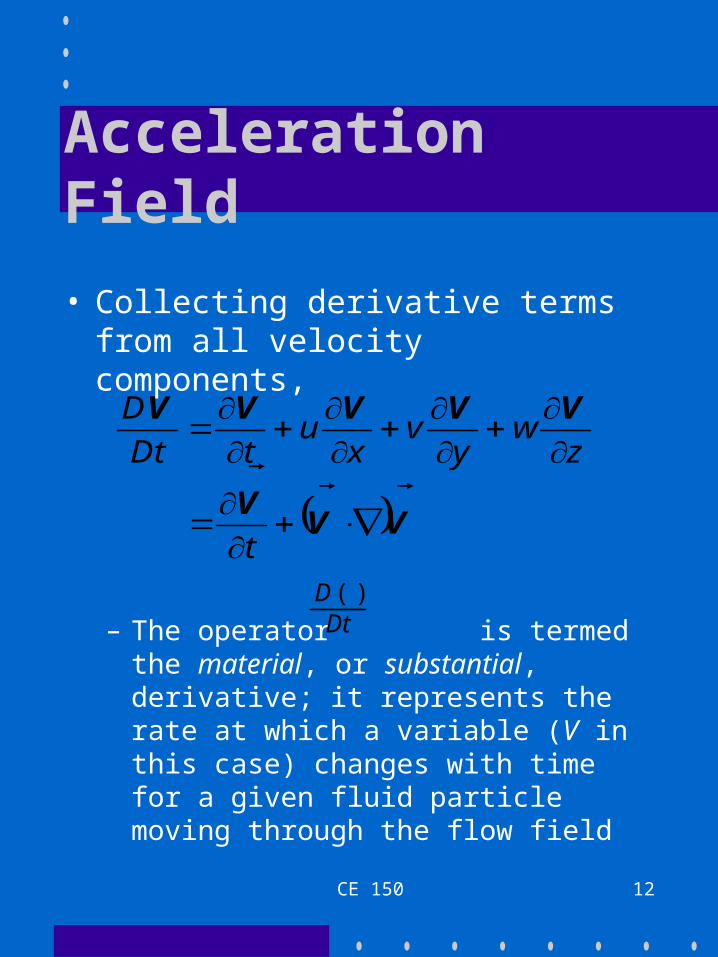
• Collecting derivative terms from all velocity components,

– The operator is termed the material, or substantial, derivative; it represents the rate at which a variable (V in this case) changes with time for a given fluid particle moving through the flow field

VVV

VVVVV

t

zw

yv

xu

tDtD

DtD ) (

CE 150 13

Acceleration Field

• The term is called the local acceleration; it represents the unsteadiness of the fluid velocity and is zero for steady flows.

• The terms are called convective accelerations; they represent the fact that the velocity of the fluid particle may vary due to the motion of the particle from one point in space to another; it can occur for both steady and unsteady flows.

tV

zyx wvu

VVV

,,

CE 150 14

The Control Volume• A control volume is a volume in space

through which fluid may flow; in some cases, the volume may move or deform

• The control volume has a boundary which separates it from the surroun-dings and defines a control surface

• In the study of fluid dynamics, the control volume approach is used to analyze fluid flow and fluid machinery

• The control volume approach is consistent with the Eulerian description

CE 150 15

The Reynolds Transport Theorem• The basic laws governing the motion

of a fluid (e.g., conservation of mass, momentum, and energy) are usually written in terms of a fixed quantity of mass, or system*

• Because a control volume does not always have constant mass, the basic laws must be rephrased

• The Reynolds Transport Theorem is a tool that allows one to shift from a system viewpoint (fixed mass) to a control volume viewpoint* In thermodynamics, a system is defined more

generally as a fixed mass or control volume

CE 150 16

The Reynolds Transport Theorem• Let B = any fluid parameter, such as

mass, velocity, temperature, momentum, etc.

• Let b = B/m, a fluid parameter per unit mass

• The mass m may be that contained in a system or a control volume

cvsys

cvcv

syssys

BB

VbdB

VbdB

CE 150 17

The Reynolds Transport Theorem• Example 4.7 (B = m, b = 1)

0

0

dt

Vdd

dtdm

dtdB

dt

Vdd

dtdm

dtdB

cvcvcv

syssyssys

CE 150 18

The Reynolds Transport Theorem

tttB

tttB

ttBttB

tB cvcvsys

)()(

)()(

III

CE 150 19

The Reynolds Transport Theorem

• Reynolds Transport Theorem (RTT) for fixed control volume with one inlet, one exit and uniform properties:

– LHS term is Lagrangian – RHS terms are Eulerian

11112222 bVAbVAt

B

BBt

BDt

DB

cv

inoutcvsys

CE 150 20

The Reynolds Transport Theorem

• A general control volume may have multiple inlets and outlets, three-dimensional flow, and nonuniform properties; the general form of the RTT is:

– for a control volume moving at constant velocity Vcv, replace V by V-Vcv

cscv

sys dAbVbdtDt

DBnV ˆ

CE 150 21

Physical Interpretation

• The RTT allows one to translate the time rate of change of some parameter B of the system in terms of the time rate of change of B of the control volume and the net flow rate of B across the control surface

• A material derivative is used because the translation consists of an unsteady term ( )/t and convective effects associated with the flow of the system across the control surface

CE 150 22

Steady Flow

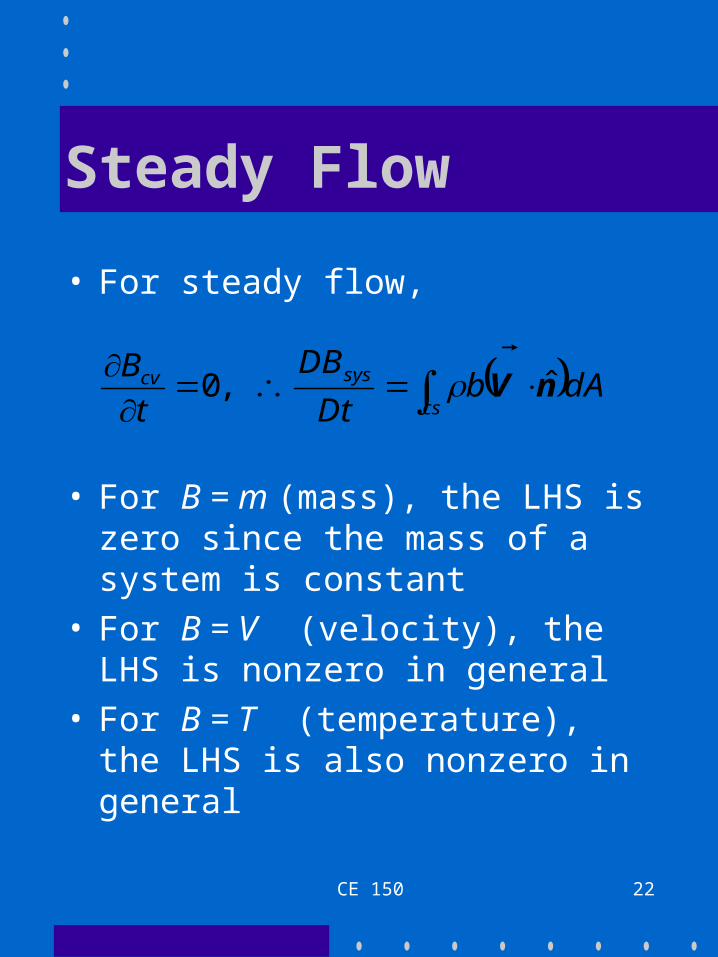
• For steady flow,

• For B = m (mass), the LHS is zero since the mass of a system is constant

• For B = V (velocity), the LHS is nonzero in general

• For B = T (temperature), the LHS is also nonzero in general

cs

syscv dAbDt

DBt

B nV ˆ ,0