University of Wisconsin MilwaukeeUWM Digital Commons

Cell and Molecular Biology iText Biological Sciences

5-4-2015

Cell and Molecular Biology: What We Know &How We Found Out (Basic iText)Gerald BergtromUniversity of Wisconsin - Milwaukee, bergtrom@uwm.edu

Follow this and additional works at: http://dc.uwm.edu/biosci_facbooks_bergtrom

This Article is brought to you for free and open access by UWM Digital Commons. It has been accepted for inclusion in Cell and Molecular BiologyiText by an authorized administrator of UWM Digital Commons. For more information, please contact gritten@uwm.edu.

Recommended CitationBergtrom, Gerald, "Cell and Molecular Biology: What We Know & How We Found Out (Basic iText)" (2015). Cell and MolecularBiology iText. Book 2.http://dc.uwm.edu/biosci_facbooks_bergtrom/2

Cell and Molecular

Biology

What We Know & How We Found Out

Gerald Bergtrom

Image Adapted From: Microarray

i

Cell and Molecular Biology What We Know & How We Found Out

A Creative Commons (Open) iText

by

Gerald Bergtrom

Page ii

Written, Compiled and Curated Under

(Creative Commons with Attribution) License

and Fair Use Rules of Distribution

Creative Commons Licensure and Permissions The following is a human-readable summary of (and not a substitute for) the license.

You are free to: Share — copy and redistribute the material in any medium or format

Adapt — remix, transform, and build upon the material for any purpose, even commercially. The licensor

cannot revoke these freedoms as long as you follow the license terms.

Under the following terms: Attribution — You must give appropriate credit, provide a link to the license, and indicate if changes

were made. You may do so in any reasonable manner, but not in any way that suggests the licensor

endorses you or your use.

No additional restrictions — You may not apply legal terms or technological measures that legally restrict

others from doing anything the license permits.

Notices: You do not have to comply with the license for elements of the material in the public domain or where your use

is permitted by an applicable exception or limitation.

No warranties are given. The license may not give you all of the permissions necessary for your intended use.

For example, other rights such as publicity, privacy, or moral rights may limit how you use the material.

Published 2015

ISBN: 978-0-9961502-0-0

Page iii

Preface

Most introductory science courses start with a discussion of scientific method, and this interactive

electronic textbook, or iText is no exception. A key feature of the iText is its focus on experimental

support for what we know about cell biology. Having a sense of how science is practiced and how

investigators think about experimental results is essential to understanding the relationship of cell

structure and function, not to mention the rest of the world around us. So we spend some time

describing the methods of cell biologists and how they are applied to experimental design. Rather

than trying to be a comprehensive reference book, the iText selectively details experiments that are

the basis of our current understanding of the biochemical and molecular basis of cell structure and

function. This focus is nowhere more obvious than in the recorded lectures (VOPs), and in your

instructor’s annotations and the graded short writing assignments in the iText. The former may

simply point to your instructor’s take on a subject, or to additional or more recent information about a

topic. The short 25 words or less writing assignments aim to strengthen critical thinking and writing

skills useful to understand science as a way of thinking… and of course, cell biology. You will likely

be discussing the underlying questions and hypotheses of experiments in class or online and at the

end of each chapter, you may even be invited to take a short objective quiz to check that they have a

good grasp of essential concepts and details. So as you use this iText, we encourage you to think

about how great experiments were inspired and designed, how alternative experimental results were

predicted, how actual data was interpreted, and finally, and what questions the investigators (and

we!) might want to ask next.

Each chapter starts with a brief introduction with links to relevant voice-over PowerPoint

presentations (VOPs). The latter add to and clarify course content, illustrating many cellular

processes with animations. To enhance accessibility, these (and all VOPs elsewhere in the iText)

are freely available on Youtubetm with optional closed captioning. Each introduction ends with a set

of specific learning objectives. These are aligned with chapter content and are intended to serve

as an aid and a guide to learning chapter content. Chapter-specific learning objectives ask students

to use new-found knowledge to make connections and demonstrate deeper concept understanding

and critical thinking skills.

While not comprehensive, this iText was written with the goal of creating content that is engaging,

free and comparable in quality to very expensive commercial textbooks. Some illustrations were

created for the iText; some were selected from online open sources (with website or other

appropriate attribution). Your instructor may upload the iText to your campus course management

system (to make it easier to use the iText and access online quizzes). Although you should find the

online iText the most efficient way to access links and complete online assignments, you are free to

download the iText so that you can read, study, and add your own annotations off-line. You can

also print out the iText and write in the margins the old fashioned way! Your instructor will

undoubtedly provide more detailed instructions for using your iText.

Page iv

Instructors Take Note: In this edition of the iText, the author’s annotations and assignments have

been removed. You are free to request this iText with the annotations alone, or with the

annotations, short assignments, one Discussion assignment and one Quiz. A smaller, easier to

download sample chapter with annotations and assignments is also available. Links to the latter two

assessments are inactive unless you create those links (and the quizzes) in your LMS. This iText is

designed to engage your students in exploring how cells work and how we figured it out. We hope

that you’ll enjoy creating and customize interactive elements in the iText and that your students will

achieve a better understanding of how scientists use skills of inductive and inferential logic to ask

questions and formulate hypotheses… and how they apply concept and method to testing those

hypotheses.

Acknowledgements

First and foremost, credit for my efforts has to go to the University of Wisconsin-Milwaukee and the

35-plus years of teaching and research experience that inform the content, concept and purpose of

this digital Open Education Resource (OER). I want to thank my colleagues in the Center for

Excellence in Teaching and Learning (CETL) and the Golda Meir Library at UW-M for the opportunity

and the critical input that led to what I have defined as an iText (interactive text). Special thanks go

to Matthew Russell, Megan Haak, Melissa Davey Castillo, Jessica Hutchings, Dylan Barth for help

and the inspiration to suggest at least a few ways to model how open course content can be made

interactive and engaging, and to Kristen Woodward and Tim Gritten for putting competent editorial

eyes on the iText.

Page v

Table of Contents

(Click title to see first page of chapter or section.)

Preface

Chapter 1: Cell Tour, Life’s Properties and Evolution, Studying Cells

Chapter 2: Basic Chemistry, Organic Chemistry and Biochemistry

Chapter 3: Details of Protein Structure

Chapter 4: Bioenergetics

Chapter 5: Enzyme Catalysis and Kinetics

Chapter 6: Glycolysis, the Krebs Cycle and the Atkins Diet

Chapter 7: Electron Transport, Oxidative Phosphorylation and Photosynthesis

Chapter 8: DNA Structure, Chromosomes, Chromatin and Replication

Chapter 9: Transcription and RNA Processing

Chapter 10: The Genetic Code and Translation

Chapter 11: Gene Regulation and Epigenetic Inheritance

Chapter 12: DNA Technologies

Chapter 13: Membrane Structure, Membrane Proteins

Chapter 14: Membrane Function

Chapter 15: The Cytoskeleton and Cell Motility

Chapter 16: Cell Division and the Cell Cycle

Videos associated with Instructor Annotations

1

Chapter 1: Cell Tour, Life’s Properties and

Evolution, Studying Cells Scientific Method; Cell structure, methods for studying cells (microscopy, cell fractionation,

functional analyses); Common ancestry, genetic variation, evolution, species diversity; cell types

& the domains of life

I. Introduction

The first two precepts of Cell Theory were enunciated near the middle of the 19th

century, after many observations of plant and animal cells revealed common structural

features (e.g., a nucleus, a wall or boundary, a common organization of cells into

groups to form multicellular structures of plants and animals and even lower life forms).

These precepts are (1) Cells are the basic unit of living things; (2) Cells can have an

independent existence. The 3rd statement of cell theory had to wait until late in the

century, when Louis Pasteur disproved notions of spontaneous generation, and German

histologists observed mitosis and meiosis, the underlying events of cell division in

eukaryotes: (3) Cells come from pre-existing cells (i.e., they reproduce)

We begin this chapter with a reminder of the scientific method, a way of thinking about

our world that emerged formally in the 17th century. We then take a tour of the cell,

reminding ourselves of basic structures and organelles. After the ‘tour’, we consider the

origin of cells from a common ancestor (the progenote) and the subsequent evolution of

cellular complexity and the incredible diversity of life forms. Finally, we consider some

of the methods we use to study cells. Since cells are small, several techniques of

microscopy, cell dissection and functional/biochemical analysis are described to

illustrate how we come to understand cell function.

Voice-Over PowerPoint Presentations

Cell Tour VOP-Part1

Cell Tour-VOP Part2

Life's Properties, Origins and Evolution VOP

Techniques for Studying Cells VOP

Learning Objectives

When you have mastered the information in this chapter and the associated VOPs, you

should be able to:

1. compare and contrast hypotheses and theories and place them and other elements

of the scientific enterprise into their place in the cycle of the scientific method.

Page 2

2. compare and contrast structures common to and that distinguish prokaryotes,

eukaryotes and archaea, and groups within these domains.

3. articulate the function of different cellular substructures and compare how

prokaryotes and eukaryotes accomplish the same functions, i.e. display the same

essential properties of life, despite the fact that prokaryotes lack most of the

structures!

4. outline a procedure to study a specific cell organelle or other substructure.

5. describe how the different structures (particularly in eukaryotic cells) relate/interact

with each other to accomplish specific functions.

6. place cellular organelles and other substructures in their evolutionary context, i.e.,

describe their origins and the selective pressures that led to their evolution.

7. distinguish between the random nature of mutation and natural selection during

evolution.

8. relate archaea to other life forms and engage in informed speculation on their origins

in evolution.

9. answer the questions “Why does evolution lead to more complex ways of sustaining

life when simpler organisms are able to do with less, and are so prolific?” & “Why

are fungi more like animals than plants?”

II. Scientific Method – The Practice of Science (click link to see Wikipedia

entry)

You can read the link at Scientific Method – The Practice of Science for a full discussion

of this topic. Here we focus on the essentials of the method and then look at how

science is practiced. As you will see, scientific method refers to a standardized

protocol for observing, asking questions about and investigating natural phenomena.

Simply put, it says look/listen, infer a cause and test your inference. But observance of

the method is not strict and is more often honored in the breach than by adherence to

protocol! As captured by the Oxford English Dictionary, the essential inviolable

commonality of all scientific practice is that it relies on “systematic observation,

measurement, and experiment, and the formulation, testing,

and modification of hypotheses."

In the end, scientific method in the actual practice of science recognizes human biases

and prejudices and allows deviations from the protocol. At its best, it provides guidance

to the investigator to balance personal bias against the leaps of intuition that successful

science requires. As followed by most scientists, the practice of scientific method would

indeed be considered a success by almost any measure. Science “as a way of

knowing” the world around us constantly tests, confirms, rejects and ultimately reveals

new knowledge, integrating that knowledge into our world view.

Page 3

Here are the key elements of the scientific method, in the usual order:

Observe natural phenomena (includes reading the science and thoughts of others).

Propose an explanation based on objectivity and reason, an inference, or

hypothesis.

An hypothesis is a declarative sentence that sounds like a fact… but isn’t! Good

hypotheses are testable - turn them into if/then (predictive) statements or yes-or-no

questions.

Design an experiment to test the hypothesis: results must be measurable evidence

for or against the hypothesis.

Perform the experiment and then observe, measure, collect data, and test for

statistical validity (where applicable).

Repeat the experiment.

Publish! Integrate your experimental results with earlier hypotheses and prior

knowledge. Shared data and experimental methods will be evaluated by other

scientists. Well-designed experiments are those that can be repeated and results

reproduced, verified and extended.

Beyond these most common parts of the scientific method, most descriptions add

two more precepts:

A Theory is a statement well-supported by experimental evidence and widely

accepted by the scientific community. Even though theories are more generally

thought of as ‘fact, they are still subject to being tested, and can even be overturned!

Scientific Laws are even closer to ‘fact’ than theories! These Laws are thought of as

universal and are most common in math and physics. In life sciences, we recognize

Mendel’s Law of Segregation and Law of Independent Assortment as much in his

honor as for their universal and enduring explanation of genetic inheritance in living

things. But we do not call these Laws facts. They are always subject to

experimental test. Astrophysicists are actively testing universally accepted laws of

physics even Mendel’s Law of Independent Assortment should not be called law

(strictly speaking) since it is not true as he stated it (go back and see how

chromosomal crossing over was found to violate this law!).

In describing how we do science, the Wikipedia entry suggests that the goal of a

scientific inquiry is to obtain knowledge in the form of testable

explanations (hypotheses) that can predict the results of future experiments. This allows

scientists to gain an understanding of reality, and later use that understanding to

intervene in its causal mechanisms (such as to cure disease). The better an hypothesis

is at making predictions, the more useful it is, and the more likely it is to be correct.

Page 4

In the last analysis, think of hypotheses as educated guesses and think of Theories

and/or Laws as one or more experimentally supported hypothesis that everyone agrees

should serve as guideposts to help us evaluate new observations and hypotheses.

Here is how Wikipedia presents the protocol of the Scientific Method:

The cycle of formulating hypotheses, testing and analyzing the results, and formulating

new hypotheses, will resemble the cycle described below:

Characterizations: observations, definitions, and measurements of the subject of

inquiry

Hypotheses: possible explanations of observations and measurements Predictions: reasoning by deductive and inferential logic from the hypothesis (note

that even widely accepted theories are subject to testing in this way)

Experiments (tests of predictions)

New Characterizations: observations, definitions, and measurements of the subject

of inquiry

A linearized, pragmatic scheme of the five points above is sometimes offered as a

guideline for proceeding:

1. Define a question

2. Gather information and resources (observe)

3. Form an explanatory hypothesis 4. Test the hypothesis by performing an experiment and collecting data in

a reproducible manner

5. Analyze the data

6. Interpret the data and draw conclusions that serve as a starting point for new

hypothesis

…To which we would add the requirement that the work of the scientist be disseminated

by publication!

III. Domains of Life

We believe with good reason (as you shall see) that all life on earth evolved from the

progenote, a cell that existed soon after the origin of life on the planet. Prokaryotes lack

nuclei (pro meaning before and karyon meaning kernel, or nucleus). Prokaryotic cells,

among the first descendants of the progenote, fall into two groups, archaea and

eubacteria (including bacteria and cyanobacteria, or blue-green algae). Prokaryotes

were long defined as a major life grouping, alongside eukaryotes. But the recent

discovery of archaea changed all that! Cells that thrive in inhospitable environments

like boiling hot springs or arctic ice were the first to be characterized as archaea, but

Page 5

now we know that these unusual organisms inhabit more temperate environments. As

of 1990, eubacteria, archaea and eukaryotes characterize the three domains of life.

That all living organisms can be shown to belong to one of these three domains has

dramatically changing our understanding of evolution.

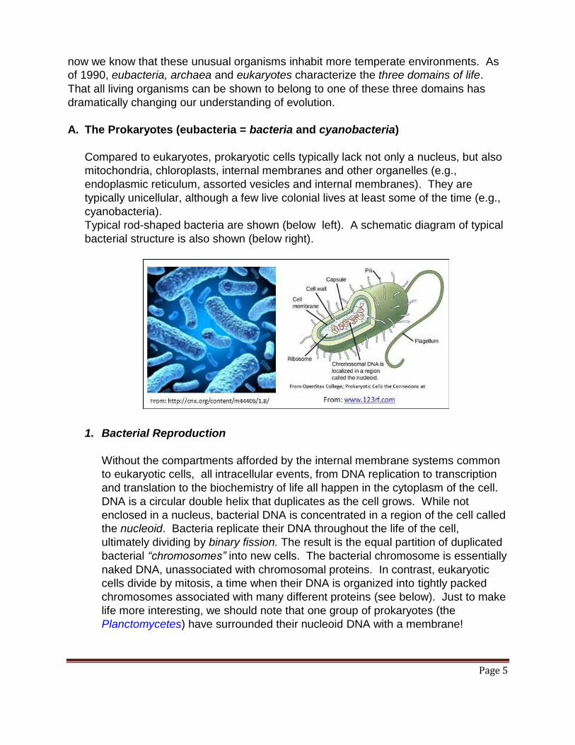
A. The Prokaryotes (eubacteria = bacteria and cyanobacteria)

Compared to eukaryotes, prokaryotic cells typically lack not only a nucleus, but also

mitochondria, chloroplasts, internal membranes and other organelles (e.g.,

endoplasmic reticulum, assorted vesicles and internal membranes). They are

typically unicellular, although a few live colonial lives at least some of the time (e.g.,

cyanobacteria).

Typical rod-shaped bacteria are shown (below left). A schematic diagram of typical

bacterial structure is also shown (below right).

1. Bacterial Reproduction

Without the compartments afforded by the internal membrane systems common

to eukaryotic cells, all intracellular events, from DNA replication to transcription

and translation to the biochemistry of life all happen in the cytoplasm of the cell.

DNA is a circular double helix that duplicates as the cell grows. While not

enclosed in a nucleus, bacterial DNA is concentrated in a region of the cell called

the nucleoid. Bacteria replicate their DNA throughout the life of the cell,

ultimately dividing by binary fission. The result is the equal partition of duplicated

bacterial “chromosomes” into new cells. The bacterial chromosome is essentially

naked DNA, unassociated with chromosomal proteins. In contrast, eukaryotic

cells divide by mitosis, a time when their DNA is organized into tightly packed

chromosomes associated with many different proteins (see below). Just to make

life more interesting, we should note that one group of prokaryotes (the

Planctomycetes) have surrounded their nucleoid DNA with a membrane!

Page 6

2. Cell Motility and the Possibility of a Cytoskeleton

Movement of bacteria is typically by chemotaxis, a response to environmental

chemicals. They can move to or away from nutrients or noxious/toxic

substances. Bacteria exhibit one of several modes of motility. For example,

many move using flagella made up largely of the protein flagellin. While the

cytoplasm of eukaryotic cells is organized by a cytoskeleton of rods and tubes

made of actin and tubulin proteins, prokaryotes were long thought not to contain

cytoskeletal analogs (never mind homologs!). However, two bacterial genes

were recently discovered and found to encode proteins homologous to eukaryotic

actin and tubulin. The MreB protein forms a cortical ring in bacteria undergoing

binary fission, similar to the actin cortical ring that pinches dividing eukaryotic

cells during cytokinesis (the actual division of a single cell into two smaller

daughter cells). This is modeled in the cross-section near the middle of a

dividing bacterium, drawn below.

The FtsZ gene encodes a homolog of tubulin proteins. Together with flagellin, the

MreB and FtsZ proteins may be part of a primitive prokaryotic cytoskeleton

involved in cell structure and motility.

3. Some Bacteria have Internal Membranes

While lacking organelles (the membrane-bound structures in eukaryotic cells),

internal membranes that appear to be inward extensions (invaginations) of

plasma membrane have been known in a few prokaryotes for some time. In

From: FtsZ_Filaments.svg

Page 7

some prokaryotic species and groups, these membranes perform capture energy

from sunlight (photosynthesis) or from inorganic molecules (chemolithotrophy).

Carboxysomes, membrane bound photosynthetic vesicles in which CO2 is

actually fixed (reduced) in cyanobacteria (shown below).

Less elaborate internal membrane systems are found in photosynthetic bacteria.

4. Bacterial Ribosomes do the Same Thing as Eukaryotic Ribosomes… and

look like them!

Ribosomes are the protein synthesizing machines of life. The ribosomes of

prokaryotes are smaller than those of eukaryotes, but in vitro they can be made

to translate eukaryotic messenger RNA (mRNA). Underlying this common basic

function is the fact that the ribosomal RNAs of all species share base sequence

and structural similarities indicating an evolutionary relationship. It was these

similarities that revealed the closer relationship of archaea to eukaryotes than

prokaryotes.

5. Bacterial Origins

You might ask which organisms came first, heterotrophic (non-photosynthetic)

bacteria or photosynthetic ones. The early earth probably favored the origin of

cells that could use environmental nutrients (i.e., carbon sources) for energy and

growth. Thus they would have been heterotrophs and perhaps some

chemoautotrophs. Using fermentative pathways similar to glycolysis,

heterotrophs would have quickly depleted their surrounding nutrients and

disappeared, save for the presence of a few rudimentary photoautotrophs

Page 8

capable of creating energy rich organic molecules using sunlight as an energy

source. While these photosynthetic cells were most likely present as mutants in

the heterotrophic population, they did not have a selective advantage until

nutrient-rich environments were depleted. This would have been because a

byproduct of photosynthesis is oxygen, a highly reactive molecule that would

have been toxic to other cells. This would have remained the case until some

heterotrophic cells evolved the biochemistry necessary to oxidize fermentation

end-products, leading to the stable carbon cycle we see today. So according to

this scenario, non-photosynthetic bacteria came first. The photosynthetic

bacterial ancestors probably evolved soon after, but it simply took some time for

them to spread and for non-photosynthetic cells to adapt to oxygen use.

In sum, prokaryotes are an incredibly diverse group of organisms, occupying

almost every wet or dry or hot or cold nook and cranny of our planet. In spite of

this diversity, all prokaryotic cells share many structural and functional metabolic

properties with each other. As we have seen with ribosomes, shared structural

and functional properties support the common ancestry of all life.

B. The Archaebacteria (Archaea)

Allessandro Volta, a physicist for whom the Volt is named, discovered methane

producing bacteria (methanogens) way back in 1776! He found them living in the

extreme environment at the bottom of Lago Maggiore, a lake shared by Italy and

Switzerland. These unusual bacteria are cheomoautotrophs that get energy from H2

and CO2 and generate methane gas in the process. It was not until the 1960s that

Thomas Brock (from the University of Wisconsin-Madison) discovered thermophilic

bacteria living at temperatures approaching 100oC in Yellowstone National Park in

Wyoming. The nickname extremophiles was soon applied to describe organisms

living in any extreme environment. One of the thermophilic bacteria, now called

Thermus Aquaticus, became the source of Taq polymerase, the heat-stable DNA

polymerase that made the polymerase chain reaction (PCR) a household name in

labs around the world!

Extremophile and “normal” bacteria both lack nuclei are similar in size and shape(s),

which initially suggested that they were closely related to bacteria and were

therefore prokaryotes (see the electron micrograph of Methanosarcina and

Pyrolobus, below). But in1977, Carl Woese compared the sequences of genes for

ribosomal RNAs in normal bacteria and an increasing number of extremophiles,

including the methanogens. Based on sequence similarities and differences, the

extremophiles seemed to form a separate group from the rest of the bacteria as well

as from eukaryotes. They were named archaebacteria, or archaea because these

organisms were thought to have evolved even before bacteria.

Page 9

Woese concluded that Archaea were a separate group, or domain of life from

bacteria and eukaryotes profoundly changing our understanding of phylogenetic

relationships. The three domains of life (Archaea, Eubacteria and Eukarya) quickly

supplanted the older division of living things into Five Kingdoms (Monera, Protista,

Fungi, Plants, and Animals). Another big surprise from rRNA gene sequence

comparisons was that the archaea were more closely related to eukaryotes than

bacteria! The evolution of the three domains is illustrated below.

Archaea contain genes and proteins as well as metabolic pathways found in

eukaryotes but not in bacteria, speaking to their closer evolutionary relationship to

eukaryotes. They also contain genes and proteins as well as metabolic pathways

unique to the group, testimony to their domain status. While some bacteria and

eukaryotes can live in extreme environments, the archaea include the most diverse

extremophiles:

Acidophiles: grow at acidic (low) pH.

Alkaliphiles: grow at high pH.

Halophiles: require high salt concentrations of salt for growth; Halobacterium

salinarium is shown below (at the left).

From: Halobacterium

Credit: James Ferry/Penn State University; Methanogen.

Page 10

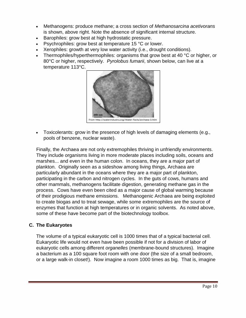
Methanogens: produce methane; a cross section of Methanosarcina acetivorans

is shown, above right. Note the absence of significant internal structure.

Barophiles: grow best at high hydrostatic pressure.

Psychrophiles: grow best at temperature 15 °C or lower.

Xerophiles: growth at very low water activity (i.e., drought conditions).

Thermophiles/hyperthermophiles: organisms that grow best at 40 °C or higher, or

80°C or higher, respectively. Pyrolobus fumarii, shown below, can live at a

temperature 113°C.

Toxicolerants: grow in the presence of high levels of damaging elements (e.g.,

pools of benzene, nuclear waste).

Finally, the Archaea are not only extremophiles thriving in unfriendly environments.

They include organisms living in more moderate places including soils, oceans and

marshes... and even in the human colon. In oceans, they are a major part of

plankton. Originally seen as a sideshow among living things, Archaea are

particularly abundant in the oceans where they are a major part of plankton,

participating in the carbon and nitrogen cycles. In the guts of cows, humans and

other mammals, methanogens facilitate digestion, generating methane gas in the

process. Cows have even been cited as a major cause of global warming because

of their prodigious methane emissions. Methanogenic Archaea are being exploited

to create biogas and to treat sewage, while some extremophiles are the source of

enzymes that function at high temperatures or in organic solvents. As noted above,

some of these have become part of the biotechnology toolbox.

C. The Eukaryotes

The volume of a typical eukaryotic cell is 1000 times that of a typical bacterial cell.

Eukaryotic life would not even have been possible if not for a division of labor of

eukaryotic cells among different organelles (membrane-bound structures). Imagine

a bacterium as a 100 square foot room with one door (the size of a small bedroom,

or a large walk-in closet!). Now imagine a room 1000 times as big. That is, imagine

Page 11

a 100,000 square foot ‘room’. Not only would you expect multiple entry and exit

doors in the eukaryotic cell membrane, but you would expect lots of interior “rooms”

with their own entry ways and exits, to make more efficient use of this large space.

The smaller prokaryotic “room” has a much larger surface area/volume ratio than a

typical eukaryotic “room”, enabling necessary environmental chemicals to enter and

quickly diffuse throughout the cytoplasm of the bacterial cell. The chemical

communication between parts of a small cell is rapid, while communication within

eukaryotic cells over a larger expanse of cytoplasm requires the coordinated

activities of subcellular components and might be expected to be slower. In fact,

eukaryotic cells have lower rates of metabolism, growth and reproduction than do

prokaryotic cells. The existence of large cells must therefore have involved an

evolution of a division of labor supported by compartmentalization. Since

prokaryotes were the first organisms on the planet, some must have evolved or

acquired membrane-bound organelles.

1. Animal and Plant cell Structure Overview

Eukaryotic cells and organisms are diverse in form but similar in function, sharing

many biochemical features with each other and as we already noted, with

prokaryotes. Typical animal and plant cells showing their organelles and other

structures are illustrated below (left and right, respectively):

Most of the internal structures and organelles of animal cells are also found in

plant cells, where they perform the same or similar functions. We begin a

consideration of the function of cellular structures and organelles with a brief

description of the function of some of these structures and organelles.

Page 12

Fungi are actually more closely related to animal than plant cells, and contain

some unique cellular structures. While fungal cells contain a wall, it is made of

chitin rather than cellulose. Chitin is the same material that makes up the

exoskeleton or arthropods (including insects and lobsters!). The organization of

fungi and fungal cells is somewhat less defined than animal cells. Structures

between cells called septa separate fungal hyphae, allowing passage of

cytoplasm and even organelles between cells. There are even primitive fungi

with few or no septa, in effect creating coenocytes that are a single giant cell with

multiple nuclei. As for flagella, they are found only in the most primitive group of

fungi.

We end this look at the domains of life by noting that, while eukaryotes are a tiny

minority of all living species, “their collective worldwide biomass is estimated at

about equal to that of prokaryotes” (Wikipedia). On the other hand, our bodies

contain 10 times as many microbial cells as human cells! In fact, it is becoming

increasingly clear that a human owes as much to its being to its microbiota as it

does to its human cells.

IV. Tour of the Eukaryotic Cell

A. Ribosomes

As noted, these are the protein synthesizing machines in the cell. They are an

evolutionarily conserved structure found in all cells, consisting of two subunits, each

made up of multiple proteins and one or more molecules of ribosomal RNA (rRNA).

Ribosomes bind to messenger RNA (mRNA) molecules and then move along the

mRNA, translating 3-base code-words (codons) and using the information to link

amino acids into polypeptides. The illustration below shows a ‘string’ group of

ribosomes, called a polyribosome or polysome for short.

Page 13

The ribosomes are each moving along the same mRNA simultaneously translating

the protein encoded by the mRNA. The granular appearance of cytoplasm in

electron micrographs is largely due to the ubiquitous distribution of ribosomal

subunits and polysomes in cells. In the electron micrographs of leaf cells from a

quiescent and an active dessert plant (Selaginella lepidophylla), you can make out

randomly distributed ribosomes/ribosomal subunits and polysomes consisting of

more organized strings of ribosomes (arrows, below left and right respectively).

Eukaryotic and prokaryotic ribosomes differ in the number of RNA and proteins in their large and small subunits, and thus in their overall size. When isolated and centrifuged in a sucrose density gradient, they move at a rate based on their size (or more specifically, their mass). Their position in the gradient is represented by an “S” value (after Svedborg, who first used these gradients to separate particles and macromolecules by mass). The illustration below shows the difference in ribosomal ‘size’, their protein composition and the number and sizes of their ribosomal RNAs.

Page 14

B. Internal membranes and the Endomembrane System

Many of the vesicles and vacuoles in cells are part of an endomembrane system, or

are produced by it. The endomembrane system participates in synthesizing and

packaging proteins dedicated to specific uses into organelles. Proteins synthesized

on the ribosomes of the rough endoplasmic reticulum and the outer nuclear

envelope membrane will enter the

interior space or lumen, or become part of the RER membrane itself. Proteins

incorporated into the RER bud off into transport vesicles that then fuse with Golgi

bodies. See some Golgi bodies (G) in the electron micrograph below.

Packaged proteins move through the endomembrane system where they undergo

different maturation steps before becoming biologically active, as illustrated below.

Some proteins produced in the endomembrane system are secreted by exocytosis.

Others end up in organelles like lysosomes. Lysosomes contain enzymes that break

Page 15

down the contents of food vacuoles that form by endocytosis. Microbodies are a

class of vesicles smaller than lysosomes, but formed by a similar process. Among

them are peroxisomes that break down toxic peroxides formed as a by-product of

cellular biochemistry.

The contractile vacuoles of freshwater protozoa expel excess water that enters cells

by osmosis; extrusomes in some protozoa release chemicals or structures that deter

predators or enable prey capture. In higher plants, most of a cell's volume is taken

up by a central vacuole, which primarily maintains its osmotic pressure. These and

other vesicles include some that do not originate in the endomembrane pathway, but

are formed when cells ingest food or other substances by the process of

endocytosis. Endocytosis occurs when the outer membrane invaginates and then

pinches off to form a vesicle containing extracellular material.

C. Nucleus

The nucleus is surrounded by a double membrane (commonly referred to as a

nuclear envelope), with pores that allow material to move in and out. As noted, the

outer membrane of the nuclear envelope is continuous with the RER (rough

endoplasmic reticulum), so that the lumen of the RER is continuous with the space

between the inner and outer nuclear membranes.

The electron micrograph of the nucleus below has a prominent nucleolus (labeled n)

and is surrounded by RER.

You can almost see the double membrane of the nuclear envelope ion this image.

Perhaps you can also make out the ribosomes looking like grains bound to the RER

Page 16

as well as to the outer membrane of the nucleus. The nucleus of eukaryotic cells

separates the DNA and its associated protein from the cell cytoplasm, and is where

the status of genes (and therefore of the proteins produced in the cell) is regulated.

Most of the more familiar RNAs (rRNA, tRNA, mRNA) are transcribed from these

genes and processed in the nucleus, and eventually exported to the cytoplasm

through nuclear pores (not visible in this micrograph). Other RNAs function in the

nucleus itself, typically participating in the regulation of gene activity. You may recall

that when chromosomes form in the run-up to mitosis or meiosis, the nuclear

envelope and nucleus disappear, eventually reappearing in the new daughter cells.

These events mark the major difference between cell division in bacteria and

eukaryotes.

In both, dividing cells must produce and partition copies of their genetic material

equally between the new daughter cells. As already noted, bacteria duplicate and

partition their naked DNA chromosomes at the same time during growth and binary

fission. Growing eukaryotic cells experience a cell cycle, within which duplication of

the genetic material (DNA replication) is completed well before cell division. The

DNA is associated with proteins as chromatin during most of the cell cycle. As the

time of cell division approaches, chromatin associates with even more proteins to

form chromosomes.

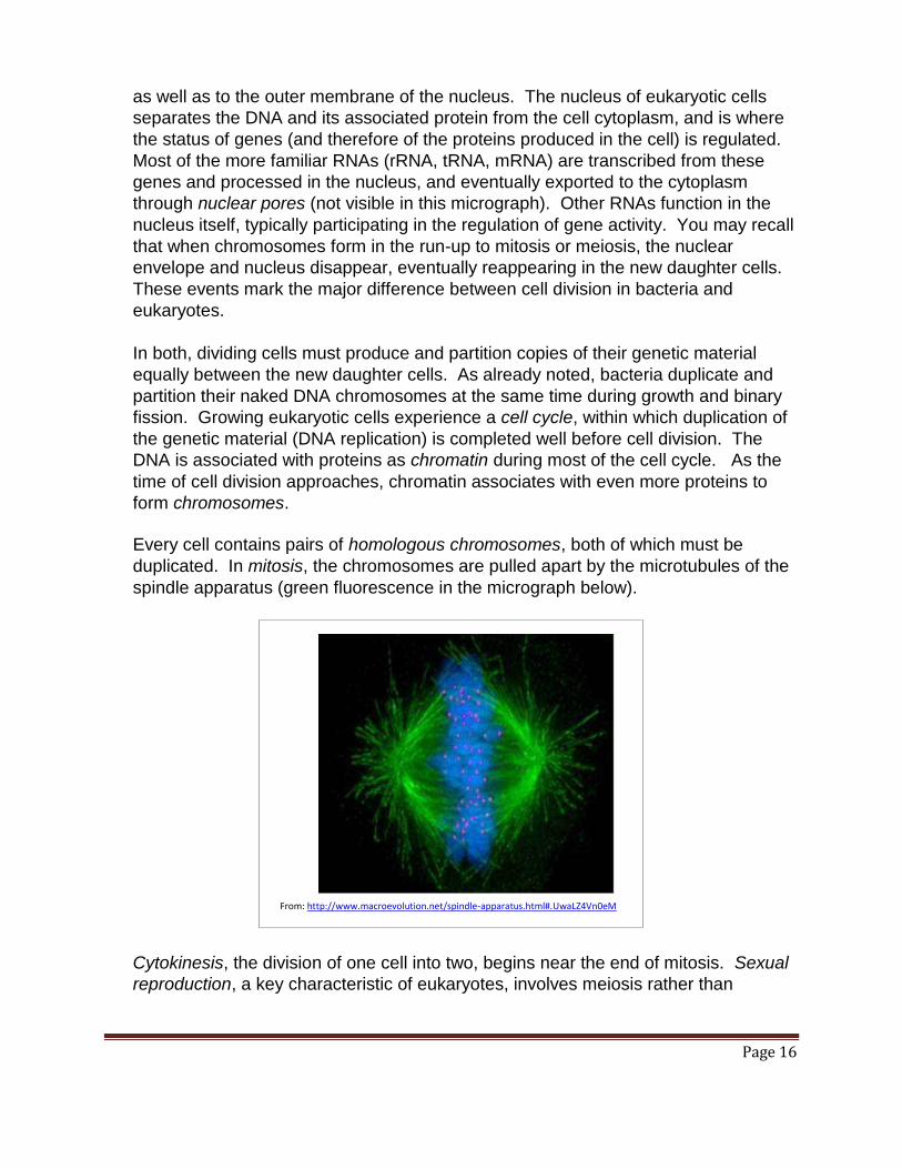
Every cell contains pairs of homologous chromosomes, both of which must be

duplicated. In mitosis, the chromosomes are pulled apart by the microtubules of the

spindle apparatus (green fluorescence in the micrograph below).

Cytokinesis, the division of one cell into two, begins near the end of mitosis. Sexual

reproduction, a key characteristic of eukaryotes, involves meiosis rather than

From: http://www.macroevolution.net/spindle-apparatus.html#.UwaLZ4Vn0eM

Page 17

mitosis. The mechanism of meiosis, the division of germ cells leading to production

of sperm and eggs, is similar to mitosis except that the ultimate daughter cells have

just one each of the parental chromosomes, eventually to become the gametes.

These aspects of cellular life are discussed in more detail elsewhere.

D. Mitochondria and Plastids

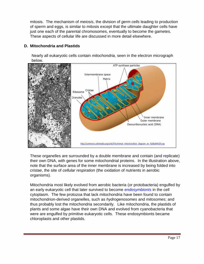
Nearly all eukaryotic cells contain mitochondria, seen in the electron micrograph

below.

These organelles are surrounded by a double membrane and contain (and replicate)

their own DNA, with genes for some mitochondrial proteins. In the illustration above,

note that the surface area of the inner membrane is increased by being folded into

cristae, the site of cellular respiration (the oxidation of nutrients in aerobic

organisms).

Mitochondria most likely evolved from aerobic bacteria (or protobacteria) engulfed by

an early eukaryotic cell that later survived to become endosymbionts in the cell

cytoplasm. The few protozoa that lack mitochondria have been found to contain

mitochondrion-derived organelles, such as hydrogenosomes and mitosomes; and

thus probably lost the mitochondria secondarily. Like mitochondria, the plastids of

plants and some algae have their own DNA and evolved from cyanobacteria that

were are engulfed by primitive eukaryotic cells. These endosymbionts became

chloroplasts and other plastids.

Page 18

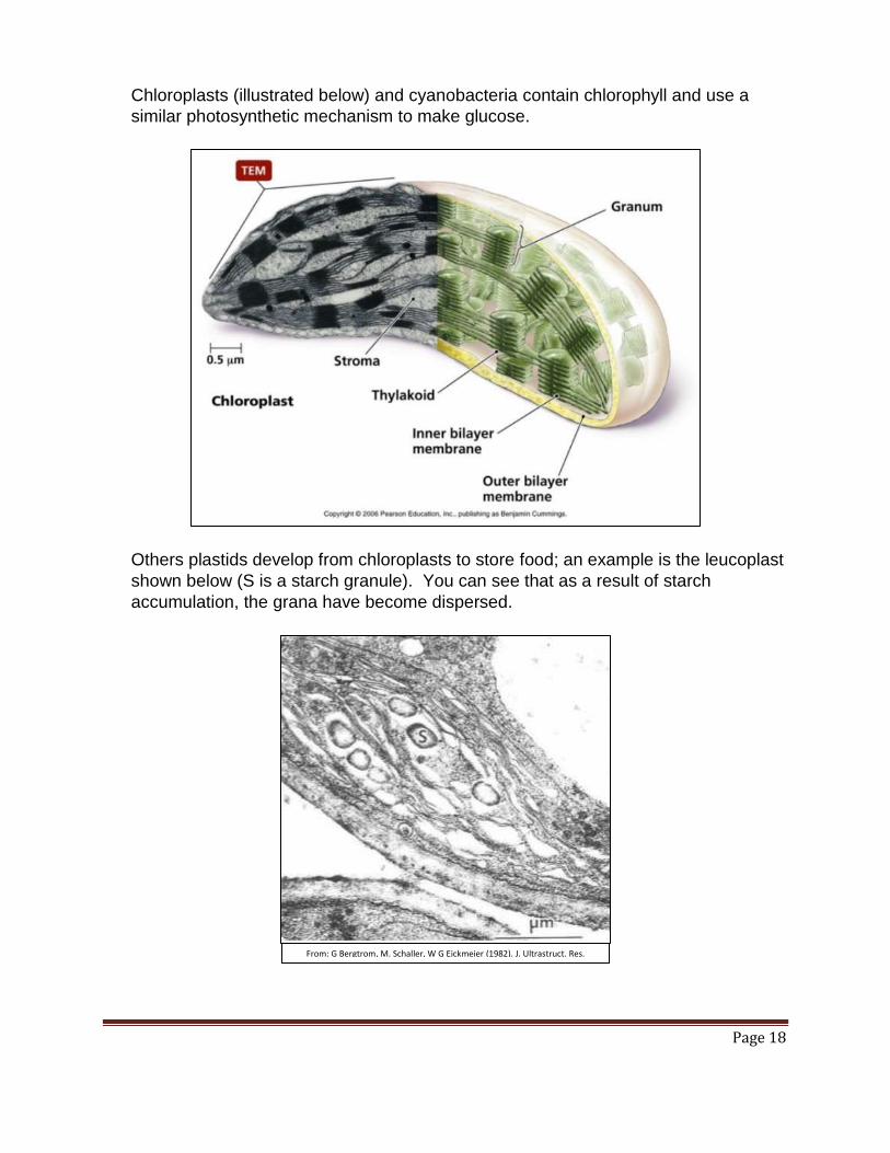
Chloroplasts (illustrated below) and cyanobacteria contain chlorophyll and use a

similar photosynthetic mechanism to make glucose.

Others plastids develop from chloroplasts to store food; an example is the leucoplast

shown below (S is a starch granule). You can see that as a result of starch

accumulation, the grana have become dispersed.

From: G Bergtrom, M. Schaller, W G Eickmeier (1982). J. Ultrastruct. Res.

78:269-282

Page 19

E. Cytoskeletal structures

We have come to understand that the cytoplasm of a eukaryotic cell is highly

structured, permeated by rods and tubules. The three main components of this

cytoskeleton are microfilaments, intermediate filaments and microtubules, with

structures illustrated below.

Microfilaments are made up of actin monomer proteins. Intermediate filament

proteins are related to keratin, the same protein found in hair, fingernails, bird

feathers, etc. Microtubules are composed of and -tubulin proteins. Cytoskeletal

rods and tubules not only determine cell shape, but also play a role in cell motility.

This includes the movement of cells from place to place and the movement of

structures within cells. We’ve already noted that a prokaryotic cytoskeleton exists

that is in part composed of proteins homologous to actins and tubulins that are

expected to play a role in maintaining or changing cell shape. Movement powered

by a bacterial flagellum relies on other proteins, notably flagellin (above). Bacterial

flagellum structures are actually attached to a molecular motor in the cell membrane

that spins a more or less rigid flagellum to propel the bacterium through a liquid

Page 20

medium. Instead of a molecular motor, eukaryotic microtubules slide past one

another causing the flagellum to undulate in wave-like motions. The motion of

eukaryotic cilia (there is no counterpart structure in prokaryote) is also based on

sliding microtubules, in this case causing the cilia to beat rather than undulate. Cilia

are involved not only in motility, but in feeding and sensation.

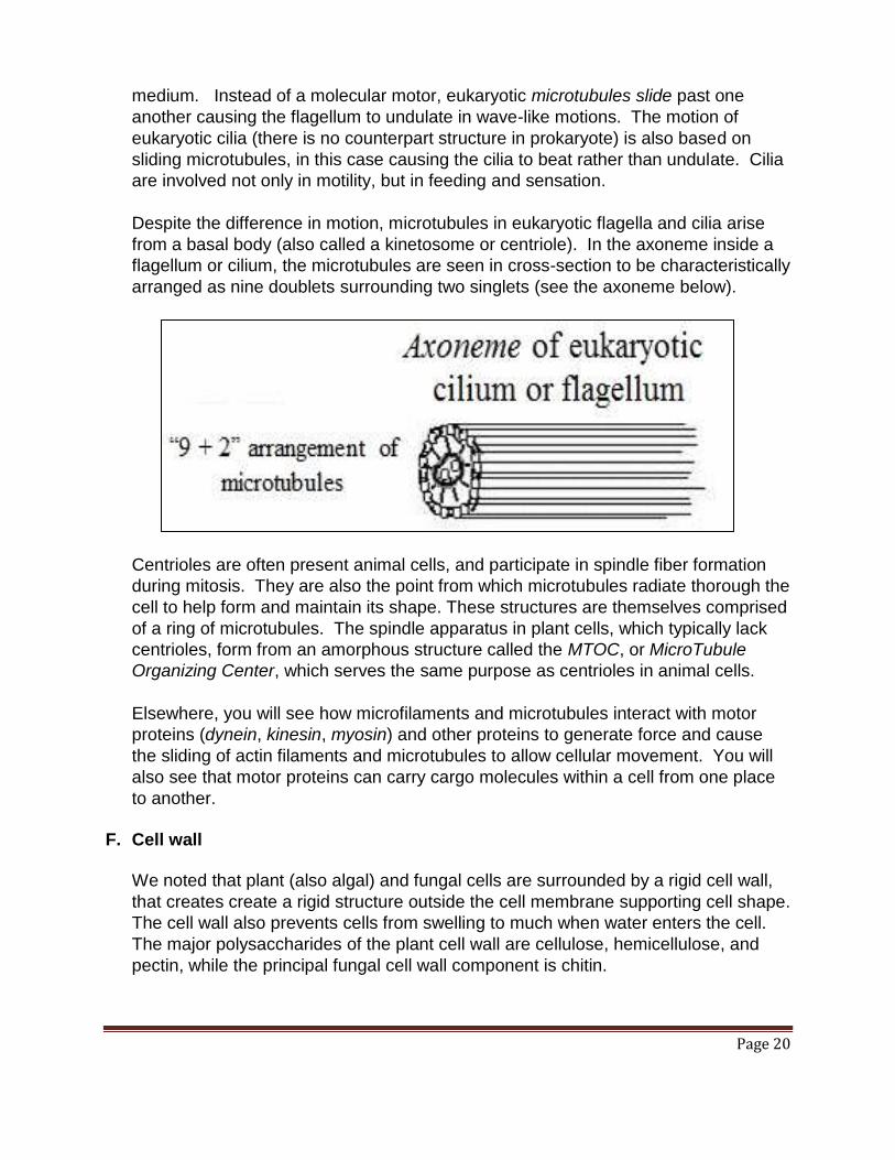
Despite the difference in motion, microtubules in eukaryotic flagella and cilia arise

from a basal body (also called a kinetosome or centriole). In the axoneme inside a

flagellum or cilium, the microtubules are seen in cross-section to be characteristically

arranged as nine doublets surrounding two singlets (see the axoneme below).

Centrioles are often present animal cells, and participate in spindle fiber formation

during mitosis. They are also the point from which microtubules radiate thorough the

cell to help form and maintain its shape. These structures are themselves comprised

of a ring of microtubules. The spindle apparatus in plant cells, which typically lack

centrioles, form from an amorphous structure called the MTOC, or MicroTubule

Organizing Center, which serves the same purpose as centrioles in animal cells.

Elsewhere, you will see how microfilaments and microtubules interact with motor

proteins (dynein, kinesin, myosin) and other proteins to generate force and cause

the sliding of actin filaments and microtubules to allow cellular movement. You will

also see that motor proteins can carry cargo molecules within a cell from one place

to another.

F. Cell wall

We noted that plant (also algal) and fungal cells are surrounded by a rigid cell wall,

that creates create a rigid structure outside the cell membrane supporting cell shape.

The cell wall also prevents cells from swelling to much when water enters the cell.

The major polysaccharides of the plant cell wall are cellulose, hemicellulose, and

pectin, while the principal fungal cell wall component is chitin.

Page 21

V. How We Know about Organelle Function A. Cell Fractionation

We could see and describe cell parts in the light or electron microscope, but we

could not definitively know their function until it became possible to release them

from cells and separate them from one another. This became possible with the

advent of differential centrifugation, a cell fractionation technique that separates

subcellular structures by differences in their mass. Cell fractionation (illustrated

below) and biochemical analysis of the isolated cell fractions were combined to

reveal what different organelles do.

Cell fractionation is a combination of various methods used to separate a cell

organelles and components. There are two phases of cell fractionation:

homogenization and centrifugation.

1. Homogenization is the process of breaking cells open. Cells are broken apart by

physical means (such as grinding in a mortar and pestle, tissue grinder or similar

device), or treatment with chemicals, enzymes, or sound waves. Some

scientists even force the cells through small spaces at high pressure to break

them apart.

Page 22

2. Centrifugation is the isolation of the cell organelles based on their different

masses. Therefore at the end of this process, a researcher has isolated the

mitochondria, the nucleus, the chloroplast, etc.

Scientists use cell fractionation to increase their knowledge of organelle functions.

To be able to do so they isolate organelles into pure groups. For example, different

cell fractions end up in the bottom of the centrifuge tubes. After re-suspension, the

pellet contents can be prepared for electron microscopy. Below are electron

micrographs of several such fractions.

The structures can be identified based (at least tentatively) based on the dimensions

and appearance of these structures. Can you tell what organelles have been

purified in each of these fractions? The functions of sub-cellular structures isolated

in this fashion were worked out by investigating their contents and testing them for

function. As an example, the structures on the left were found in a low speed

centrifugal pellet, implying that they are large structures. They look a bit like nuclei,

which are in fact the largest structures in a eukaryotic cell. If you wanted to be sure,

what biochemical or functional test might you do to confirm that the structures in the

left panel were indeed nuclei? This method has already resulted in our

understanding not only of the identity of subcellular structures, but of previously un-

noticed functions of many if not all cell organelles.

For a detailed description of the biochemical analysis, review your instructors VOP

and/or un-narrated presentation on cell fractionation. This course is devoted to

understanding cell structure and function and how prokaryotic and eukaryotic cells

(and organisms) use their common biochemical inheritance to meet very different

survival strategies. As you progress in the course, you will encounter one of the

recurring themes involving the dissection of cells. Look for this theme, involving the

isolation and analysis of function of the cell components, and where possible, the re-

assembly (reconstitution) of cellular structures and systems.

From: openi.nlm.nih.gov From: Isolated RER From: Isolated Golgi vesicles

From: Isolated Mitochondria

Page 23

IV. Evolution, Speciation and the Diversity of Life

Natural selection was Charles Darwin’s theory for how evolution led to the diversity of

species on earth. New species arise when beneficial traits are naturally selected from

genetically different individuals in a population, with the concomitant culling of less fit

individuals from populations over time. If natural selection acts on individuals, evolution

results from the persistence and spread of selected, heritable changes through

successive generations in a population. Evolution is reflected as an increase in

diversity at all levels of biological organization, from species to individual organisms to

molecules like DNA and proteins.

Life on earth originated and then evolved from a universal common ancestor some 3.7

billion years ago. Repeated speciation, the continual divergence of life forms from this

ancestor (the progenote) through natural selection and evolution is supported the

shared biochemistry we have already noted (the ‘unity’ of life) and for more closely

related organisms, by shared morphological traits. Since the revolution in molecular

biology, shared gene and other DNA sequences have confirmed shared ancestry of

diverse organisms across all three of life’s domains, and where we have them, across

species represented in the fossil record. Morphological, biochemical and genetic traits

that are shared across species are defined as homologous, and can be used to

reconstruct evolutionary histories. The biodiversity that environmentalists (and

scientists in general)) try to protect has resulted from millions of years of speciation and

by extinction. It needs protection from evolutionary processes that are accelerating in

human hands!

Let’s take a closer look at the biochemical and genetic unity among livings things.

Albert Kluyver first recognized that cells and organisms vary in form appearance in spite

of the essential biochemical unity of all organisms (http://en.wikipedia.org/wiki/Albert

Kluyver). We’ve already considered some of the consequences cells getting larger in

evolution when we tried to explain how larger cells divided their labors among smaller

intracellular structure (organelles). When eukaryotic cells evolved into multicellular

organisms, it became necessary for the different cells to communicate with each other

in addition to being able to respond to environmental cues. Some cells evolved

mechanisms to “talk” directly to adjacent cells and others evolved to transmit electrical

(neural) signals to other cells and tissues. Still other cells produced hormones to

communicate with cells to which they had no physical attachment. As species

diversified to live in very different habitats, they also evolved very different nutritional

requirements, along with more extensive and elaborate biochemical pathways to digest

their nutrients and capture their chemical energy. Nevertheless, Kluyver and many

others eventually recognized that despite billions of years of obvious evolution and

astonishing diversification, the underlying genetics and biochemistry of living things on

this planet is remarkably unchanged. This unity amidst the diversity of life is an

apparent paradox of life that we will probe in this course.

Page 24

A. Genetic Variation, the Basis of Natural Selection, Leads to Evolution

DNA contains the genetic instructions for the structure and function of cells and

organisms. When and where a cell or organism’s genetic instructions are used (i.e.,

to make RNA and proteins) is regulated. Genetic variation results from random

mutations. Genetic diversity arising from mutations is in turn, the basis of evolution.

B. The Genome: an organisms complete genetic instructions

The genome of an organism is the entirety of its genetic material (DNA or for some

viruses, RNA). Through mutation, genomes exhibit genetic variation, not only

between species, but between individuals of the same species.

C. All Organisms Alive Today Descended from a Common Ancestor

Living things were once divided into 5 kingdoms. This classification has been

replaced by 3 domains of life. All life originated from a common ancestor, the

progenote. While the progenote is often defined as the first cell, it should be seen

not so much as a single cell, but as a single population of related cells. If life

originated more than once (as seems likely), there would probably have been

several different kinds of cells that reproduced to create different populations of

cells, each increasing in size and accumulating mutations that led eventually to

speciation. Some of these populations of cells were early evolutionary dead ends

that disappeared through extinction. Then one such population survived and

underwent speciation driven by natural selection. Even among these surviving

species descended from the same original cell, many would also have gone extinct

(e.g., like dinosaurs). Apparently, the progeny of progeny of these other

populations could not compete for resources and eventually died out. This left

some descendants of the progenote evolving, eventually resulting in the organisms

alive today.

V. Microscopy Reveals Life’s Diversity of Structure and Form

For a gallery of light, fluorescence and transmission and scanning electron

micrographs, check out this site (compare these with PowerPoint lecture images):

Gallery of Micrographs

Light microscopy reveals much of cellular diversity (The Optical Microscope).

Check this site through the section on fluorescence microscopy. Click on links to

different kinds of light microscopy to see sample micrographs of cell and tissue

samples. Also check micrographs and corresponding Drawings of Mitosis

section for a reminder of how eukaryotic cells divide.

Page 25

Confocal microscopy is a special form of fluorescence microscopy that enables

imaging through thick samples and sections. The result is often 3D-like, with

much greater depth of focus than other light microscope methods. Click at

Gallery of Confocal Microscopy Images to see a variety of confocal micrographs

and related images; look mainly at the specimens.

Transmission electron microscopy (TEM) achieves more power and resolution

than any form of light microscopy (Transmission Electron Microscopy). Together

with biochemical and molecular biological studies continues to reveal how

different cell components work with each other (see cell fractionation, below).

The higher voltage in High Voltage Electron microscopy is an adaptation that

allows TEM through thicker sections than regular (low voltage) TEM. The result

is micrographs with greater resolution and contrast.

Scanning Electron Microscopy (SEM) allows us to examine the surfaces of

tissues, small organisms like insects, and even of cells and organelles (Scanning

Electron Microscopy; check this web site through Magnification for a description

of scanning EM, and look at the gallery of SEM images at the end of the entry).

Some iText & VOP Key words and Terms Actin Eukaryotes Nuclear pores

Archaea Eukaryotic flagella Nucleoid

Bacterial cell walls Evolution nucleolus

Bacterial Flagella Exocytosis Nucleus

Binary fission Extinction Optical microscopy

Cell fractionation Hypothesis Plant cell walls

Cell theory Inference Plasmid

Chloroplasts Intermediate filaments Progenote

chromatin keratin Prokaryotes

Chromosomes Kingdoms Properties of life

Cilia Lysosomes Rough endoplasmic reticulum

Confocal microscopy Meiosis Scanning electron microscopy

Cytoplasm Microbodies Scientific method

Cytoskeleton Microfilaments Secretion vesicles

Cytosol Microtubules Smooth endoplasmic reticulum

Deduction Mitochondria Speciation

Differential centrifugation Mitosis Theory

Page 26

Diversity Motor proteins Tonoplast

Domains of life Mutation Transmission electron microscopy

Dynein Natural selection Tubulins

Endomembrane system Nuclear envelope

Page 27

Chapter 2: Basic Chemistry, Organic Chemistry

and Biochemistry Basic chemistry (chemical bonding (covalent, polar covalent, ionic, H-bonds; Water

properties, water chemistry, pH); Organic molecules and Biochemistry (chemical

groups, monomers, polymers, condensation and hydrolysis); Macromolecules

(polysaccharides, lipids, polypeptides & proteins, DNA, RNA)

I. Introduction

In this chapter we review basic chemistry from atomic structure to molecular bonds to

the structure and properties of water, followed by a review of key principles of organic

chemistry - the chemistry of carbon-based molecules. We’ll see how the polar covalent

structure of water explains virtually all properties of water from the energy required to

melt or vaporize a gram of water to its surface tension to its ability to hold heat… not to

mention its ability to dissolve a wide variety of solutes from salts to proteins and other

macromolecules. We’ll distinguish hydrophilic interactions from water’s hydrophobic

interactions with lipids and fatty components of molecules. Finally, we’ll review some

basic biochemistry. We’ll look common reactions by which small monomers get linked

to form large polymers (macromolecules) like polysaccharides, polypeptides and

polynucleotides (DNA, RNA). We’ll also see the reactions that break macromolecules

down to their constituent monomers. For example amylose, a component of starch, is a

large simple homopolymer of repeating glucose monomers. Polypeptides are

heteropolymers of 20 different amino acids, while the DNA and RNA nucleic acids are

heteropolymers made using only 4 different nucleotides. So, when we eat a meal, we

digest the plant or animal polymers back down to monomers by a process called

hydrolysis. In hydrolysis, a water molecule is ‘added’ across the bonds linking the

monomers in the polymer. When the monomeric digestion products get into our cells,

they can be assembled into our own macromolecules by removing those water

molecules, the process called condensation, or dehydration. While fats (triglycerides)

and phospholipids are not (strictly speaking) macromolecules, we’ll see that they

breakdown and form by hydrolysis and condensation, respectively. Fats are of course

an important energy molecule, and phospholipids, chemical relatives of fats that are the

basis of cellular membrane structure.

Many cellular structures are based on macromolecules interacting with each other via

many relatively weak bonds (H-bonds, electrostatic interactions, Van der Waals forces).

Even the two complementary DNA strands are held in a stable double helix by millions

Page 28

of H-bonds between the bases in the nucleotides in opposite chains. Monomers also

serve other purposes related to energy metabolism, cell signaling etc. The links to

websites (mostly Wikipedia) on atoms and basic chemistry are more detailed than

required for this course, but depending on your chemistry background, you may find

“googling” these subjects interesting and useful. Of course, use the VOPs and/or the

un-narrated PowerPoints as the guide to what you must understand about the basic

chemistry and biochemistry presented here.

Voice-Over PowerPoint Presentations

Chemistry and the Molecules of Life VOP Biochemistry Part1: Carbohydrates, Lipids & Proteins VOP Biochemistry Part2: DNA, RNA, Macromolecular Assembly VOP

Learning Objectives

When you have mastered the information in this chapter and the associated VOPs, you

should be able to:

1. compare and contrast the definitions of atom, element and molecule.

2. articulate the difference between energy and position-based atomic models and the

behavior of sub-atomic particles that can absorb energy from and release energy to

the environment.

3. state the difference between atomic shells and orbitals.

4. state the difference between kinetic and potential energy and how it applies to atoms

and molecules.

5. explain the behavior of atoms or molecules that fluoresce when excited by high-

energy radiation, and those that don’t.

6. be able to distinguish between polar and non-polar covalent bonds between atoms

in molecules, and their physical-chemical properties.

7. predict the behavior of electrons in compounds held together by ionic interactions.

8. predict the behavior of highly soluble and insoluble salts when placed in water and

explain that behavior in atomic/molecular terms.

9. compare and contrast the different properties of water and explain how water’s

atomic/molecular structure supports these properties.

10. draw monomers and show how they undergo dehydration synthesis to form linkages

in polymers.

11. distinguish between chemical “bonds” and “linkages” in polymers.

12. categorize different bonds on the basis of their strengths.

13. place hydrolytic and dehydration synthetic reactions in a metabolic context.

Page 29

II. Atoms and Basic Chemistry

A. Overview of Elements and Atoms

Let’s first deal with the difference between elements and atoms, which are often

confused in casual conversation! Both terms describe matter, substances with

mass. The atom is the fundamental unit of matter. Every atom consists of a nucleus

surrounded by a cloud of electrons in motion. The different elements are different

kinds of matter distinguished by different physical and chemical properties. These

properties are in turn defined by differences in the mass and structure of their atoms,

i.e., the number of protons and neutrons in the nucleus and the arrangement of the

orbiting electrons. The nuclei of atoms of most elements contain positively charged

protons and uncharged (electrically neutral) neutrons; the exception is hydrogen,

whose most stable atoms lack neutrons. Electrons are negatively charged and are

maintained in their atomic orbits because of electromagnetic forces created in part

by their attraction to the positively charged nuclei. Protons and neutrons account for

most of the mass of atoms. They are about 2000X (more precisely, between 1836X-

1839X) more massive than electrons.

The same electromagnetic forces that keep electrons orbiting their nuclei may cause

atoms to combine to form molecules in which atoms are linked by chemical bonds.

Whether or not a given element can form chemical bonds with another element is

determined by the unique mass and structure of their atoms. Recall that atoms are

physically most stable when they are electrically uncharged, with an equal number of

protons and electrons. But atoms of the same element can have a different number

of neutrons. Isotopes are atoms of the same element with different than the usual

number of neutrons. For example, the most abundant isotope of hydrogen contains

one proton and one electron. The nucleus of the hydrogen isotope deuterium

contains a neutron; tritium contains 2 additional neutrons. While some isotopes may

be less stable than others (tritium is radioactive and subject to nuclear decay over

time), they all share the same chemical properties and behave the same way in

chemical reactions. In chemical interactions, some atoms can gain or lose

electrons, becoming charged ions; atoms do not lose protons or neutrons as a result

of chemical interactions. Up to two electrons move in a space defined as an orbital.

In addition to occupying different areas around the nucleus, electrons exist at

different energy levels, moving with different kinetic energies. Electrons can also

absorb or lose energy, jumping or falling between energy levels. The number and

arrangement of electrons in the atoms of an element ultimately determine its

Page 30

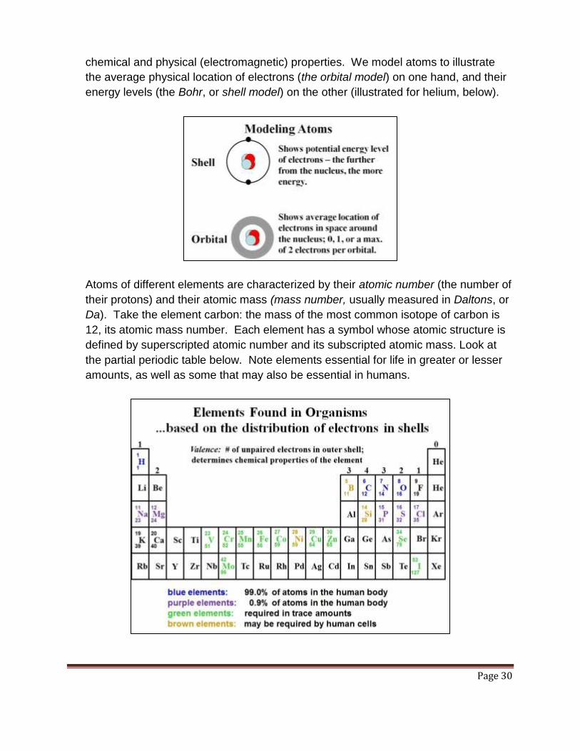
chemical and physical (electromagnetic) properties. We model atoms to illustrate

the average physical location of electrons (the orbital model) on one hand, and their

energy levels (the Bohr, or shell model) on the other (illustrated for helium, below).

Atoms of different elements are characterized by their atomic number (the number of

their protons) and their atomic mass (mass number, usually measured in Daltons, or

Da). Take the element carbon: the mass of the most common isotope of carbon is

12, its atomic mass number. Each element has a symbol whose atomic structure is

defined by superscripted atomic number and its subscripted atomic mass. Look at

the partial periodic table below. Note elements essential for life in greater or lesser

amounts, as well as some that may also be essential in humans.

Page 31

B. Electron Configuration – Shells and Subshells

The Bohr model of the atom allows a convenient way to think about the kinetic

energy of electrons, and how electrons can absorb and release energy. The shells

indicate the energy levels of electrons. Typically, beaming radiation (visible or UV

light for example) at atoms can excite electrons. Electrons can absorb energy

(radiation, light, electrical). If an electron absorbs a full quantum of energy (or

photon radiant energy) it will be excited from the ground state (the shell it normally

occupies) into a higher shell. Having absorbed this energy, the electron now moves

at greater speed around the nucleus. Thus the excited electron has more kinetic

energy than it did ‘at ground’ (below).

Excited electrons are unstable, and will eventually return to their ground state (and

their lower energy shell). The ground state is sometimes also called the ’resting

state’, but electrons at ground are by no means resting! They simply move with less

kinetic energy than when excited. Since electrons are more stable at ground state,

excited electrons will release some of the energy they originally absorbed. In most

cases, this energy is released as heat. But in some cases, they will release the

energy as light. Atoms and molecules whose excited electrons release visible light

as they return to ground state are called fluorescent. The most obvious example of

this phenomenon is the fluorescent light fixture in which electrical energy excites

electrons out of atoms in molecules coating the interior surface of the bulb. As all

those excited electrons return to ground state (only to be re-excited again), they

release the fluorescent light. As we shall see, biologists and chemists have turned

fluorescence into a tool of biochemistry, molecular biology and microscopy.

Page 32

III. Chemical bonds

Atoms combine to make molecules by forming bonds. Covalent bonds are strong

bonds. They involve unequal or equal sharing of electrons, leading to polar covalent

bonds vs. non-polar covalent bonds respectively. Ionic bonds are weaker than

covalent bonds. They are created by electrostatic interactions between elements that

gain or lose electrons. Hydrogen (H-) bonds are in a class by themselves! These

electrostatic interactions account for the physical and chemical properties of water and

are involved in the interactions between and within molecules and macromolecules.

We’ll look more closely at these bonds and see how even the weak bonds are essential

to life.

A. Covalent Bonds

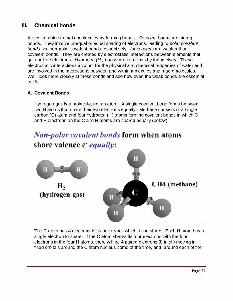
Hydrogen gas is a molecule, not an atom! A single covalent bond forms between

two H atoms that share their two electrons equally. Methane consists of a single

carbon (C) atom and four hydrogen (H) atoms forming covalent bonds in which C

and H electrons on the C and H atoms are shared equally (below).

The C atom has 4 electrons in its outer shell which it can share. Each H atom has a

single electron to share. If the C atom shares its four electrons with the four

electrons in the four H atoms, there will be 4 paired electrons (8 in all) moving in

filled orbitals around the C atom nucleus some of the time, and around each of the

Page 33

H atomic nuclei some of the time. In effect, the outer shell of the C atom and each

of the H atoms are filled at least some of the time. This stabilizes the molecule;

recall that atoms are most stable when their outer shells are filled and each electron

orbital is filled (i.e., with a pair of electrons). The bonds in methane and hydrogen

gas are non-polar covalent bonds because the electrons in the bonds are shared

equally.

If the nuclei of atoms in a molecule are more different in size that C and H, the

electrons in the bonds might not be shared equally. This is the case with water

(shown below).

The larger nucleus of the oxygen atom in H2O attracts electrons more strongly than

the two H atoms, so that the shared electrons spend more of their time around the O

atom. Compare the position of the paired electrons in water with those in hydrogen

gas or methane). Such bonds are called polar covalent bonds because the O atom

will carry a partial negative charge while each of the H atoms will carry a partial

positive charge. The partial charges are indicated by the Greek letter delta (). The

polar covalent nature of water allows it to interact with other polar molecules and

with itself. In the illustration, the partial (and opposite) charges of two water

molecules attract each other. The polar covalent nature of water goes a long way to

explaining the physical and chemical properties of water… and why water is

essential to life on this planet!

Page 34

Both polar and non-polar covalent bonds play a major role on the structure of

macromolecules, like insulin, the protein hormone shown below.

A space-filling model of the hexameric form of stored insulin on the left emphasizes

its tertiary structure based on X-Ray crystallography… that is, how the structure

might look if you could actually see it. The so-called ribbon diagram on the right

highlights regions of internal secondary structure within the protein. When secreted

from Islets of Langerhans cells in the pancreas, active insulin is a dimer of two

polypeptides, shown here in turquoise and dark blue. Almost hidden towards the

lower left of the illustration are the two disulfide bridges (yellow “V”s) holding

together the two polypeptides. Except for these two covalent disulfide bonds, insulin

subunit structure and the interactions holding the subunits together are based on

many electrostatic interactions (including H-bonds) and other weak interactions,

Protein structure is covered in more detail in a separate chapter.

For more about covalent bonds, see About Covalent Bonds (from Wikipedia).

http://commons.wikimedia.org/wiki/File:InsulinMonomer.jpg

Page 35

B. Ionic Bonds

When atoms gain or lose electrons, they form ions, so by definition, ions carry either

a negative or positive charge. Ions are produced when atoms can obtain a stable

number of electrons by giving up or gaining electrons. Common table salt is a good

example (illustrated below).

Na (sodium) can donate a single electron to Cl (chlorine) generating Na+ and Cl-.

The ion pair is held together in crystal salt by the electrostatic interaction of opposite

charges.

IV. A Close Look at Water Chemistry

A. Hydrogen Bonds, the Polarity and Properties of Water

Hydrogen bonds are a subcategory of electrostatic interaction (i.e., formed by the

attraction of oppositely charges). As noted above, water molecules cohere (stick to

one another) because of strong electrostatic interactions that form H-bonds. These

interactions lead to the formation of hydrogen bonds, or H-bonds. Another

consequence of water’s polar covalent nature is that it is a good solvent because it is

attracted to other charged molecules and molecular surfaces. In doing so, the water

molecules typically form H-bonds with the dissolving molecules. Water-soluble

molecules or molecular surfaces that are attracted to water are referred to as

hydrophilic. Lipids like fats and oils are not polar molecules and therefore that do

not dissolve in water; they are hydrophobic.

When soluble salts like NaCl are mixed with water, the salt dissolves because the Cl-

and Na+ ions are more strongly attracted to the partial positive and negative charges

(respectively) of multiple water molecules. The result is that the ions separate as

they dissolve. We call this separation of salt ionization.

Page 36

The dissolution of NaCl in water is an example of the solvent properties of water

(shown below).

Water is also a good solvent for macromolecules (proteins, nucleic acids) with

exposed polar chemical groups on their surfaces. These charged groups attract

water molecules as shown below.

Page 37

In addition to being a good solvent, we define the following properties of water:

Cohesion: the ability of water molecules to stick together via hydrogen bonds (H-

bonds).

High Surface tension: water’s high cohesion means that it can be hard to break

the surface (think the water strider insect that “walks’ on water.

Adhesion: the ability of water to form electrostatic interactions with ions and other

polar covalent molecules.

High specific heat: water’s cohesive properties are so strong that it takes a lot of

energy to heat water (1 Kcal, or Calorie, with a capital C) to heat a gram of water

by 1oC.

High heat of vaporization: It takes even more energy/gram of water to turn it into

water vapor!

In fact, all of these properties of water are based on its polar nature and H-bonding

abilities that attract other water molecules as well as ions and other polar molecules.

B. Water Ionization and pH

One last property of water – it can ionize, forming H+ and OH- ions or more correctly,

pairs of water molecules form H3O+ and OH- ions. When an acid is added to water,

H+ ions (in fact, protons!) dissociate from the acid molecule, increasing the number

of H3O+ ions in the solution. Acidic solutions have a pH below 7.0 (neutrality). When

bases are added to water, they ionize and release OH- (hydroxyl) ions which remove

H+ ions (protons) from the solution, raising the pH of the solution. To review the

basics of acid-base chemistry:

When dissolved in water,

• Acids release H+

• Bases accept H+

Since the pH of a solution is the negative logarithm of the hydrogen ion

concentration,

• at pH 7.0, a solution is neutral

• below a pH of 7.0, a solution is acidic

• above a pH of 7.0, a solution is basic

Page 38

V. Some Basic Biochemistry: Monomers and Polymers; the

Synthesis and Degradation of Macromolecules

The common themes for how living things build and break down macromolecules

involve dehydration (or condensation) and hydrolysis reactions, respectively. One

reaction is essentially the reverse of the other, as illustrated below:

Dehydration synthesis (condensation) reactions build macromolecules by removing a

water molecule from the interacting molecules. The forward reaction between two

amino acids (below left) forms a peptide bond (or peptide linkage) between the amino

acids (below right).

Hydrolysis reactions involve the addition of water molecules across linkages connecting

monomers or other molecular groups. The hydrolysis of peptide linkages, shown as the

reverse reaction in the illustration, would happen in your stomach and small intestines

after a protein-containing meal.

Condensation reactions are key reactions in the synthesis of large molecules

(macromolecules like polypeptides, polysaccharides, DNA, RNA, etc.). Glucose is a

monomer of starch in plant and glycogen in animals. We build proteins from amino

acids and we synthesize nucleic acids (DNA and RNA) from nucleotide monomers.

Page 39

Even fats and membrane phospholipids are built from smaller components in

condensation reactions. When we eat a meal, we digest the macromolecules in food

back down to monomers by hydrolysis. That’s how our cells get to finish the job of

turning a cow or turnip into you and me! For more detail, check out other chapters in

this text and see the links below:

About Glucose and its Polymers (from Wikipedia)

About Amino Acids and Polypeptides (from Wikipedia)

Nucleotides and Nucleic Acids (from Wikipedia)

About Fats (from Wikipedia)

About Phospholipids (from Wikipedia)

Some iText & VOP Key Words and Terms

acids and bases hydrogen bonds photon

adhesion hydrolysis polar covalent bonds

amino acids hydrophilic polymers

atom hydrophobic polynucleotides

atomic mass ionic bonds polypeptides

Bohr model ionization polysaccharides

Carbohydrates isotopes potential energy

cohesion kinetic energy properties of water

dehydration synthesis lipids protons

digestion macromolecules quantum

DNA molecule RNA

electron shell monomers salts

electrons neutrons scanning tunneling microscope

electrostatic interaction nucleotides sharing electrons

element orbitals solutes

Ester linkage partial charge specific heat

excitation peptide linkage surface tension

fats pH triglycerides

fluorescence phospholipids valence

glycoside linkage phosphate ester linkage Van der Waals forces

heat of vaporization phosphodiester linkage water ions

water of hydration

Page 40

Chapter 3: Details of Protein Structure Protein Structure and Configuration: Primary, Secondary, Tertiary, Quaternary;

Protein Folding, Domains and Motifs, Studying Proteins

I. Introduction

Proteins are the work-horses of cells. Comprised of one or more polypeptides, they:

are the catalysts that make biochemical reactions possible,

are components of membranes that selectively let substances into and out of the

cell,

are the basis of a cells ability to respond to changes in the environment and more

generally to communicate with one another,

form the internal structure (cytoskeleton) of cells

allow cells to move and muscles to contract…

are in fact responsible for many other cell functions!

In this chapter, we look at the different levels of protein structure and what it takes to be

a functional protein. The primary (1o) structure of a polypeptide is its amino acid

sequence. Amino acid interactions near each other in the sequence cause the

polypeptide to fold into its secondary (2o) structure ( helix, -, or pleated sheet).

Tertiary (3o) structure forms when the polypeptide further folds into more a complex 3-

dimensional structure. The accurate folding of a polypeptide into a correct and active

molecule is typically mediated by other proteins (called chaperones!). Tertiary structure

is the result of many non-covalent interactions occasionally stabilized by covalent bond

formation between amino acid side-chains at some distance from one another in the

primary sequence. Quaternary (4o) structure refers to proteins made up of two or more

polypeptide subunits. Finally, some proteins associate with metal ions (e.g., Mg++, Mn++)

or small organic molecules (e.g., heme) before they become functionally active. Finally,

we’ll look at some techniques for studying protein structure.

As with any discussion of molecular (especially macromolecular) function, a recurring

theme emerges: the function of a protein depends on its conformation - that is, the

location of critical functional groups (usually amino acid side chains) and their charge

configuration. Conformation or shape defined this way accounts for what other

molecules a protein can interact with. Watch for this theme as we look at enzymes

catalysis, the movement of molecules in and out of cells, the response of cells their

environment, the ability of cells and organelles to move, DNA replication, gene

transcription and regulation, protein synthesis and more.

Voice-Over PowerPoint Presentations

Protein Structure & Function VOP

How We Study Proteins VOP

Page 41

Learning Objectives

When you have mastered the information in this chapter and the associated VOPs, you

should be able to:

1. distinguish between the orders of protein structure based on the atomic and

molecular interactions responsible for each order.

2. differentiate beta sheet, alpha helix and random coil structure based on the atomic

interactions involved on each.

3. formulate an hypothesis for why the amino acid glycine is a disruptor of alpha helical

polypeptide structure.

4. compare and contrast motif and domain structure of proteins and polypeptides, and

their contribution to protein function.

5. describe different techniques for studying proteins and the physical/chemical

differences between proteins that make each technique possible.

6. explain the relationship between shape/configuration, cell function and

communication, and the notion of molecular communication.

II. Protein Structure

Refer to the 4 levels of protein structure below as you continue to explore them in detail.

An fold into

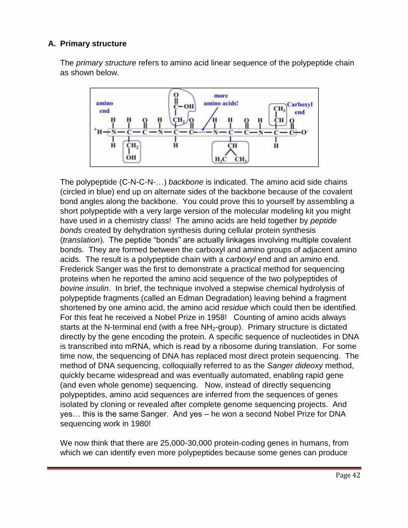
Page 42

A. Primary structure

The primary structure refers to amino acid linear sequence of the polypeptide chain

as shown below.

The polypeptide (C-N-C-N-…) backbone is indicated. The amino acid side chains

(circled in blue) end up on alternate sides of the backbone because of the covalent

bond angles along the backbone. You could prove this to yourself by assembling a

short polypeptide with a very large version of the molecular modeling kit you might

have used in a chemistry class! The amino acids are held together by peptide

bonds created by dehydration synthesis during cellular protein synthesis

(translation). The peptide “bonds” are actually linkages involving multiple covalent

bonds. They are formed between the carboxyl and amino groups of adjacent amino

acids. The result is a polypeptide chain with a carboxyl end and an amino end.

Frederick Sanger was the first to demonstrate a practical method for sequencing

proteins when he reported the amino acid sequence of the two polypeptides of

bovine insulin. In brief, the technique involved a stepwise chemical hydrolysis of

polypeptide fragments (called an Edman Degradation) leaving behind a fragment

shortened by one amino acid, the amino acid residue which could then be identified.

For this feat he received a Nobel Prize in 1958! Counting of amino acids always

starts at the N-terminal end (with a free NH2-group). Primary structure is dictated

directly by the gene encoding the protein. A specific sequence of nucleotides in DNA

is transcribed into mRNA, which is read by a ribosome during translation. For some

time now, the sequencing of DNA has replaced most direct protein sequencing. The

method of DNA sequencing, colloquially referred to as the Sanger dideoxy method,

quickly became widespread and was eventually automated, enabling rapid gene

(and even whole genome) sequencing. Now, instead of directly sequencing

polypeptides, amino acid sequences are inferred from the sequences of genes

isolated by cloning or revealed after complete genome sequencing projects. And

yes… this is the same Sanger. And yes – he won a second Nobel Prize for DNA

sequencing work in 1980!

We now think that there are 25,000-30,000 protein-coding genes in humans, from

which we can identify even more polypeptides because some genes can produce

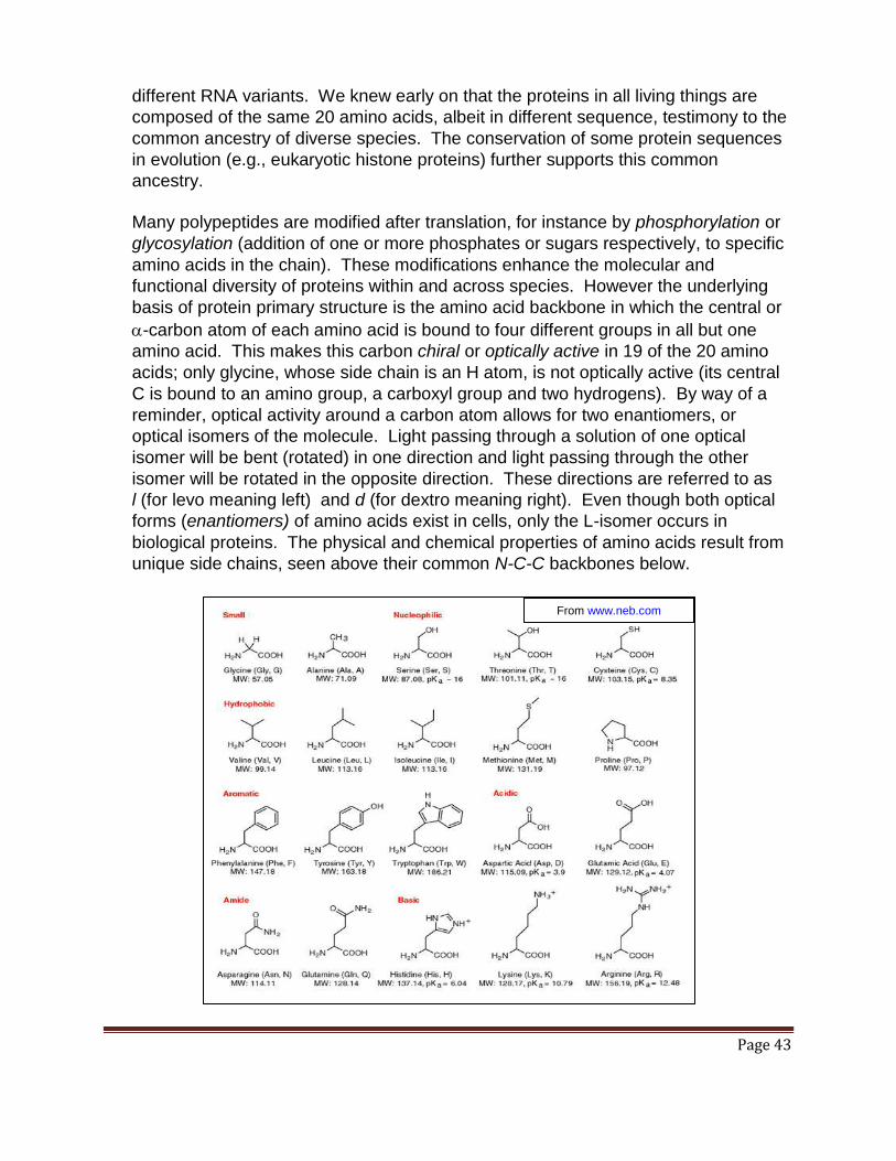
Page 43

different RNA variants. We knew early on that the proteins in all living things are

composed of the same 20 amino acids, albeit in different sequence, testimony to the

common ancestry of diverse species. The conservation of some protein sequences

in evolution (e.g., eukaryotic histone proteins) further supports this common

ancestry.

Many polypeptides are modified after translation, for instance by phosphorylation or

glycosylation (addition of one or more phosphates or sugars respectively, to specific

amino acids in the chain). These modifications enhance the molecular and

functional diversity of proteins within and across species. However the underlying

basis of protein primary structure is the amino acid backbone in which the central or

-carbon atom of each amino acid is bound to four different groups in all but one

amino acid. This makes this carbon chiral or optically active in 19 of the 20 amino

acids; only glycine, whose side chain is an H atom, is not optically active (its central

C is bound to an amino group, a carboxyl group and two hydrogens). By way of a

reminder, optical activity around a carbon atom allows for two enantiomers, or

optical isomers of the molecule. Light passing through a solution of one optical

isomer will be bent (rotated) in one direction and light passing through the other

isomer will be rotated in the opposite direction. These directions are referred to as

l (for levo meaning left) and d (for dextro meaning right). Even though both optical

forms (enantiomers) of amino acids exist in cells, only the L-isomer occurs in

biological proteins. The physical and chemical properties of amino acids result from

unique side chains, seen above their common N-C-C backbones below.

From www.neb.com

Page 44

In turn, the unique physical and chemical properties of proteins are determined by

the interaction of amino acid side chains within a polypeptide and between

polypeptides.

B. Secondary structure

Secondary structure refers to highly regular local structures within a polypeptide (

helix) and either within or between polypeptides ( sheets). These two types of

secondary structure were suggested in 1951 by Linus Pauling and coworkers.

These conformations occur due to the spontaneous formation of hydrogen bonds

between the main-chain peptide groups, as shown in the two left panels in the

drawing below.

The helix or sheets form based on which configuration of hydrogen bonds is

most stable. Some parts of a polypeptide may not form either helices or sheets, but

are instead lengths of less structured amino acids called random coils; these

typically connect more structured regions of the molecule. All three of these

elements of secondary structure can occur in a single polypeptide or protein, as

shown at the right in the illustration above. The pleated sheets are indicated as

ribbons with arrow heads representing N-to-C or C-to-N polarity of the sheets. As

you can see, a pair of peptide regions forming a pleated sheet may do so in either

the parallel or antiparallel directions (look at the arrowheads of the ribbons), which

will depend on other influences dictating protein folding to form tertiary structure.

C. Tertiary structure

When polypeptides fold into more 3-dimensional shapes, they are said to have

tertiary structure. The helix or sheets are folded and incorporated into globular

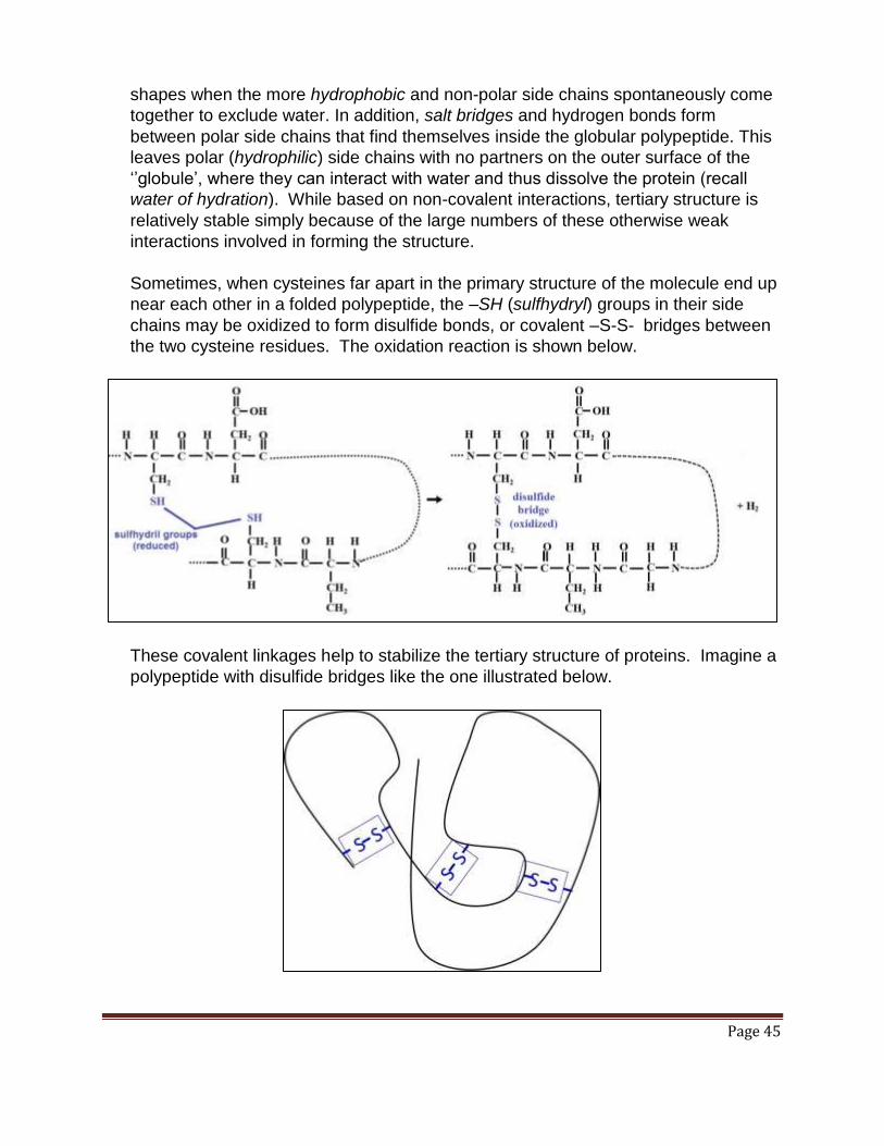
Page 45

shapes when the more hydrophobic and non-polar side chains spontaneously come

together to exclude water. In addition, salt bridges and hydrogen bonds form

between polar side chains that find themselves inside the globular polypeptide. This

leaves polar (hydrophilic) side chains with no partners on the outer surface of the

‘’globule’, where they can interact with water and thus dissolve the protein (recall

water of hydration). While based on non-covalent interactions, tertiary structure is

relatively stable simply because of the large numbers of these otherwise weak

interactions involved in forming the structure.

Sometimes, when cysteines far apart in the primary structure of the molecule end up

near each other in a folded polypeptide, the –SH (sulfhydryl) groups in their side

chains may be oxidized to form disulfide bonds, or covalent –S-S- bridges between

the two cysteine residues. The oxidation reaction is shown below.

These covalent linkages help to stabilize the tertiary structure of proteins. Imagine a

polypeptide with disulfide bridges like the one illustrated below.

Page 46

Now imagine a changing environment surrounding the protein. Blood is a good

example. Changing the temperature or salt concentration surrounding a protein

might disrupt some of the non-covalent bonds maintaining the shape of the active

protein. But the disulfide bridges limit the disruption and enable the protein to fold

correctly when conditions return to normal (think homeostasis!). Proteins with

disulfide bonds are more common in extracellular proteins (e.g., those in the

circulatory system). Because the cytosol is typically a reducing environment

cysteines in proteins tend to be reduced, remaining in the sulfhydryl (–SH) state.

D. Quaternary structure

Quaternary structure is the three-dimensional structure of a protein composed of two

or more polypeptides. In this context, the quaternary structure is stabilized by the

same non-covalent interactions and disulfide bonds as the tertiary structure. Proteins

with quaternary are called multimers. Specifically, a dimer contains two

polypeptides, a trimer contains three polypeptides, a tetramer if it contains four

polypeptides and so on. Multimers made up of identical subunits are referred to with

a prefix of "homo-" (e.g. a homotetramer). Those made up of different subunits are

heteromers. The vertebrate hemoglobin molecule, consisting of - and two -

globins (shown below) is a heterotetramer.

E. Some proteins require prosthetic Groups to be biologically active

Hemoglobins exemplify another feature of the structure of many proteins. To be

biologically active, globin polypeptides must associate with a prosthetic group, in this

case a cyclic organic molecule called heme. At the center of each heme is the iron

which reversibly binds oxygen. Hemoglobins are found in all kinds of organisms,

from bacteria to plants and animals… even some anaerobic organisms). Other

proteins must be bound to different metal ions (magnesium, manganese, cobalt…)

to be biologically active.

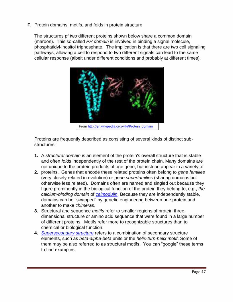
Page 47

F. Protein domains, motifs, and folds in protein structure

The structures pf two different proteins shown below share a common domain

(maroon). This so-called PH domain is involved in binding a signal molecule,

phosphatidyl-inositol triphosphate. The implication is that there are two cell signaling

pathways, allowing a cell to respond to two different signals can lead to the same

cellular response (albeit under different conditions and probably at different times).

Proteins are frequently described as consisting of several kinds of distinct sub-

structures:

1. A structural domain is an element of the protein's overall structure that is stable

and often folds independently of the rest of the protein chain. Many domains are

not unique to the protein products of one gene, but instead appear in a variety of

2. proteins. Genes that encode these related proteins often belong to gene families

(very closely related in evolution) or gene superfamilies (sharing domains but

otherwise less related). Domains often are named and singled out because they

figure prominently in the biological function of the protein they belong to, e.g., the

calcium-binding domain of calmodulin. Because they are independently stable,

domains can be "swapped" by genetic engineering between one protein and

another to make chimeras.

3. Structural and sequence motifs refer to smaller regions of protein three-

dimensional structure or amino acid sequence that were found in a large number

of different proteins. Motifs refer more to recognizable structures than to

chemical or biological function.

4. Supersecondary structure refers to a combination of secondary structure

elements, such as beta-alpha-beta units or the helix-turn-helix motif. Some of

them may be also referred to as structural motifs. You can “google” these terms

to find examples.

From http://en.wikipedia.org/wiki/Protein_domain

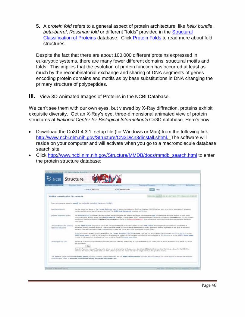
Page 48

5. A protein fold refers to a general aspect of protein architecture, like helix bundle,

beta-barrel, Rossman fold or different "folds" provided in the Structural

Classification of Proteins database. Click Protein Folds to read more about fold

structures.

Despite the fact that there are about 100,000 different proteins expressed in

eukaryotic systems, there are many fewer different domains, structural motifs and

folds. This implies that the evolution of protein function has occurred at least as

much by the recombinatorial exchange and sharing of DNA segments of genes

encoding protein domains and motifs as by base substitutions in DNA changing the

primary structure of polypeptides.

III. View 3D Animated Images of Proteins in the NCBI Database.

We can’t see them with our own eyes, but viewed by X-Ray diffraction, proteins exhibit

exquisite diversity. Get an X-Ray’s eye, three-dimensional animated view of protein

structures at National Center for Biological Information’s Cn3D database. Here’s how:

Download the Cn3D-4.3.1_setup file (for Windows or Mac) from the following link:

http://www.ncbi.nlm.nih.gov/Structure/CN3D/cn3dinstall.shtml. The software will

reside on your computer and will activate when you go to a macromolecule database

search site.

Click http://www.ncbi.nlm.nih.gov/Structure/MMDB/docs/mmdb_search.html to enter

the protein structure database:

Page 49

The search example shown above for human insulin takes you to this link:

http://www.ncbi.nlm.nih.gov/structure/?term=human+insulin&SITE=NcbiHome&subm

it.x=12&submit.y=12 The website is shown below:

Click View in Cn3D for the desired protein. For human insulin see this:

To rotate the molecule, click View then Animation, then Spin… and enjoy!

Page 50

Key Words and Terms

alpha helix hydrophobic interactions random coil

amino acid residues levels of protein structure recombinatorial exchange

-carbon orders of protein structure salt bridges

beta barrel peptide bonds secondary structure

beta sheet peptide linkages sequence motifs

chaperones phosphorylation side chains

configuration pleated sheet structural domain

disulfide bonds polypeptide backbone structural motif

functional groups primary structure sulfhydryl groups

glycosylation protein folding tertiary structure

helix-turn-helix motif quaternary structure

Page 51

Chapter 4: Bioenergetics Thermodynamics (Free Energy, Enthalpy and Entropy), Chemical Energy,

Open vs. Closed Systems

I. Introduction

The Laws of Thermodynamics describe the flow and transfer of energy in the universe.

The 3 Laws are:

1. Energy can neither be created nor destroyed.

2. Universal entropy (disorder) is always increasing.

3. Entropy declines with temperature -as temperatures approach absolute zero, so

does entropy.

In living systems we do not have to worry about the 3rd law. But as we’ll see, equations

for energy exchange in living systems reflect the temperature dependence of entropy

changes during reactions. In this chapter we’ll look how we come to understand basic

thermodynamic principles and how they apply to living systems (bioenergetics). First

we’ll look at different kinds of energy and how redox reactions govern the flow of energy

through living things. Then we’ll try to understand some simple arithmetic statements of

the Laws of Thermodynamics for closed systems and see how they apply to chemical

reactions conducted under so-called standard conditions. Finally, since there really is

no such thing a s a closed system, we’ll look at energetics (energy transfers) in open

systems.

Learning Objectives

When you have mastered the information in this chapter and the associated VOPs, you

should be able to:

1. explain the difference between energy transfer and energy transduction.

2. compare and contrast different kinds of energy (e.g., mass, heat light, etc.)

3. derive the algebraic relationship between free energy, enthalpy and entropy.

4. predict changes in free energy based on changes in the concentrations of reactants

and products in closed systems and open systems.

5. explain the reciprocal changes in universal free energy and entropy.

6. articulate the difference between reactions that are exothermic, endothermic,

exergonic, and endergonic.

7. predict whether a biochemical reaction will release free energy if it is exothermic,

and if so, under what conditions.

8. distinguish between chemical equilibrium and steady-state reaction conditions.

9. compare and contrast the same reaction under conditions where it is endergonic and

conditions where it releases free energy.

Voice-Over PowerPoint Presentations

Bioenergetics Part1 VOP

Bioenergetics Part2 VOP

Page 52

II. Kinds of Energy

We can easily recognize different kinds of energy around us like heat, light, electrical,

chemical, nuclear, sound, etc… and you probably know that energy is measurable

(calories, joules, volts, decibels, quanta, photons…). Even mass is a form of energy, as

you may recall from Albert Einstein’s famous e=mc2 equation (the law of relativity). The

problem in thinking about thermodynamics is that the universe is big and there are too

many kinds of energy to contemplate at once! Let’s try to simplify by imagining only two

kinds of energy in the universe: potential energy and kinetic energy. The best known

example of these two kinds of energy may be water above a dam, representing

potential energy. When the water flows over the dam, the potential energy is released

as kinetic energy. In the old days the kinetic energy of flowing water could be converted

into the kinetic energy of a millstone to grind flower or other grains. These days, if water

flows through a hydroelectric dam, the water’s kinetic energy can be converted

(transduced) into electricity. In this simple view, heat (molecular motion), electricity (a

current of electrons), sound (waves), and light (waves OR moving ‘particles’) are

different forms of kinetic energy. The energy of mass, or its position in the universe is

potential energy. Thus chemical energy, e.g., the energy in a mole of ATP is potential

energy. Physicists talk a lot about potential and kinetic energy flow and conversion.

An equally simple but more general way to conceptualize energy is as useful vs.

useless. This concept led directly to the arithmetic formulation of the thermodynamic

laws. In this binary way of thinking about energy, useless energy is entropy, while

useful energy can be any of the other forms of energy (potential or kinetic).

We will see that the key to understanding bioenergetics is to understand the difference

between closed systems and open systems in the universe. Systems that reach

equilibrium (like biochemical reaction in a test tube) are considered closed systems.

Closed systems are artificial, possible only in a lab where one can restrict and measure

the amount of energy and mass getting into or escaping the system. Cells, living things

in general, and basically every reaction or event in the rest of the universe (outside the

lab) are open systems that readily exchange energy and mass with their surroundings.

With this brief introduction, we can put ourselves in the position of early scientists trying

to understand energy flow in the universe. Let’s look at the thermodynamic laws and

how they apply to living systems (bioenergetics). As we go through this exercise, let’s

remember that the Laws of Thermodynamics can be demonstrated because all kinds

of energy can be measured (heat in calories or joules, electricity in volts, light in quanta,

matter in units of mass, etc.).

Page 53

III. Deriving simple energy relationships

A. Energy in the Universe: the Universe is a Closed System

Consider an event, or happening. We can agree, I think, that when stuff happens,

participants in the happening go from an unstable state to a relatively more stable

state. In a simple example you carrying a bag of marbles and you accidentally tipped

over the bag. The marbles would fall to the floor and roll and spread out, eventually

coming to a stop. At that point, the marbles are in a more stable state than they

were when you were holding the bag. If asked, you would say that gravity made the

marbles fall from the bag. That is certainly true. But couldn’t you also agree that the

drive to greater stability is what made the marbles fall? In fact, it is indeed the drive

to greater stability that makes things happen! This is the essence of the 2nd law of

thermodynamics - all universal energy transfer events occur with an increase in

stability…, that is, an increase in entropy.

Let’s accept that the tendency of things go from unstable to more stable is a natural,

rational state of affairs…, like those marbles on the floor, or a messy bedroom with

clothes strewn about. So, we can say that messy and disordered is more stable

than ordered. Of course marbles dropping or clothing going from folded and hung

onto the floor releases energy (potential energy) as they fall (kinetic energy). If you

don’t believe that this release of energy is real, just think of how much energy you

will need to pick up the marbles and fold your clothes (after laundering them of

course!). Let’s model the flow of energy in the universe that is consistent with

thermodynamic laws.

If energy can be neither created nor destroyed, a simple statement of the First Law

could be:

Euniversal = Elight + Eheat + Eelectrical + Emass....

The equation sums up the different kinds of energy in the universe. Look at it this

way:

Page 54

Energy cannot get in or out of the universe. It can only be transferred between parts

or converted from one form to another. It follows then that Euniversal is the sum of all

kinds of energy in the universe, and must be a constant, or:

Elight + Eheat + Eelectrical + Emass +… = a constant This is a statement of the First Law. If we go with the simpler binary notion or useful

and useless energy, our equation can be re-written as the sum of just two kinds of

energy in the universe:

Euniversal = Guniversal + TSuniversal where G is useful energy (“Gibbs” free energy ), S is useless energy (entropy), and

T is absolute temperature (included because of the 3rd law).

This is also a statement of the First Law. Here is our revised circle diagram:

In this binary energy model, it follows that as universal entropy increases, free

energy in the universe must decrease:

Free or ‘potentially useful’ energy is higher in more ordered, complex and therefore

relatively unstable systems. Free energy will be released spontaneously (without

help) from unstable, ordered systems.

Page 55

B. Energy is Exchange between Systems in the Universe

If we can measure the amount of energy put into or removed from a system within

the universe, we can write a more useful equation to follow the transfer of energy

between a system and its surroundings:

H = G + TS where H = change (in enthalpy, i.e., as energy entering/leaving the system in

units of heat energy); G = change in free energy; S= change in entropy, T =

absolute temperature (oK). Note that changes in entropy are often referred to as

heat lost in a reaction or physical event, and can therefore be easily confused with

enthalpy change!

According to this equation H = G + TS, interacting systems in our universe

would seem to be closed systems. Accordingly, if energy is put into or removed

from the system (H), it will be exactly balanced by increases and/or decreases in

the other two terms (G + TS). We refer to these systems as closed systems not

because they are really closed, but because we can isolate them well enough to

account for energy flow into and out of the system.

For any algebraic equation with three variables, if you know two of the values, you

can calculate the third! Here is a simple situation to illustrate the point: If I put a

liter of water on a burner and light the flame the water gets hot. If the temperature

of the liter of water rises by 1oC, we know that it has absorbed 1000 calories (one

Kcal, or one food Calorie) of the heat from the burner.

Since energy interactions depend on different physical conditions, such as

temperature and air pressure, we need to standardize those conditions when

conducting experiments that measure energy changes in those isolated (“closed”

systems. Now let’s apply this equation to chemical reactions that occur in cells.

Because most life on earth lives at sea level where the air pressure is 1 atmosphere

and the temperature is in the 20’s (Celsius), typical determinations of H, G, and

S are made under standard conditions where T=298oK (25oC), an atmospheric

pressure of pressures of 1 atm, a constant pH of 7.0. In addition, measured energy

values are corrected to be for molar quantities of reactants. Our equation for

reactions under these standard conditions becomes: H = G0 + TS where G0

is the standard free energy change for the reaction conducted in a closed system

under standard conditions, H is still the enthalpy change and S is still the entropy

change… but determined under unimolar and standard conditions.

But wait… what’s this about unimolar conditions? That just means if you are

burning glucose in a calorimeter, you would burn say 180 milligrams of the stuff and

Page 56

then multiply the calories released (H) by 1000 to get how much heat would be

released if you actually burned a whole mole (180 gm) of the stuff. So, what is the

molecular weight of glucose? How much does a mole of glucose weigh? How

much glucose was actually burned in the calorimeter, in moles? Now we are ready

to consider examples of how we determine the energetics of reactions.

C. How is Enthalpy Change (H) Determined?

H for a chemical reaction can easily be determined by conducting the reaction

under standard conditions in a bomb calorimeter. Food manufacturers determine

the calorie content of food using a bomb calorimeter. As the reaction takes place (in

the beaker in the illustration) it will either release or absorb heat. The water in the

calorimeter jacket will either get warmer or cooler, as measured by the thermometer.

A reaction that releases heat as it reaches equilibrium is exothermic that by

definition will have a negative H. For example, if the package says that a chocolate

bar has 90 Calories, then the bar will generate 90 kilocalories of heat when it is

burned in the calorimeter. (1 Calorie, with a capital C = 1000 calories, or 1 Kcal; 1

calorie is the energy needed to raise a gram of water by 1oC). On the other hand,

some chemical reactions actually absorb heat. Just take a hospital cold-pack,

squeeze it to get it going and toss it in the calorimeter. You can watch the

temperature in the calorimeter drop as the pack absorbs heat from the surroundings!

Such reactions are defined as endothermic. A bomb calorimeter schematic is

shown below.

Listen to an animated description of calorimetry at http://youtu.be/cpps2CZ0aA4.

OK, so we can determine the value of one of the energy parameters… we need to know

at least one other, either Go or S before the equation H = G0 + TS becomes

useful.

Page 57

D. How is Standard Free Energy change (G0) Determined?

The standard free energy change, G0, is directly proportional to the

concentrations of reactants and products of a reaction conducted to completion (i.e.,

equilibrium) under standard conditions. So to determine G0 we need to be able to

measure the concentration of reactants and reaction products before and after a

chemical reaction (i.e., when the reaction reaches equilibrium). For example, take

the following generic chemical reaction:

2A + B <====> 2C + D

It turns out that G0 is related to the equilibrium concentrations of A, B, C and D by

the following equation:

G0 = -RTlnKeq = RTln [C]2[D]

[A]2[B]

This is the Boltzman equation, where R= the gas constant (1.806 cal/mole-deg), T

= 298oK and Keq is the equilibrium constant. As you can see, the Keq for the

reaction is the ratio of the product of the concentrations of the products (raised to

their stoichiometric powers) to the product of the concentrations of the reactants

raised to their stoichiometric powers.

The Boltzman equation allows us to calculate G0, the standard free energy change

for a reaction, provided you can determine the equilibrium concentrations of

reactants and products in a chemical reaction. Consider the following generic

chemical reaction:

If the G0 is a negative number, the reaction releases free energy and is defined as

exergonic. If the G0 Is a positive number, the reaction absorbs free energy and is

defined as endergonic.

E. Working an Example Using these Equations for Closed Systems

Consider the following reaction:

Is this reaction endergonic or exergonic? How would you know, even without

determining G0?

You can also do the math: after measuring (assaying) the concentrations of the

reactants and products for this reaction, they are found to be:

[X] = 2,500 cal/Mole; [Y] = 500 Kcal/Mole

A + B C + D

X Y

Page 58

Use the Boltzmann equation to calculate the standard free energy for this reaction.

What is the Keq for this reaction? What is the G0 for the reaction? If you did not

come up with a Keq of 0.2 and an absolute value for the standard free energy |G0| of 866.2 cal/mole, re-calculate or collaborate with a classmate. Based on the actual

(not the absolute) value of G0 is this reaction endergonic or exergonic?

Let’s assume that when the reaction is conducted in a bomb calorimeter, the

reaction proceeded to equilibrium with a H = 2800 calories/Mole. Together with the

enthalpy change, it is now possible to calculate S for a reaction. Assume that the

H is 1,800 Kcal/mole and based on your determination for G0, calculate the S for

the reaction. At equilibrium, did the reaction proceed with an increase or decrease

in entropy under standard conditions?

F. Actual Free Energy Change in Open Systems

Later, we will be discussing the flow of energy through living things, from sunlight to

chemical energy in nutrient molecules to the extraction of this chemical energy as

ATP and heat, to the performance of all manner of cellular work. Cells are open

systems, able to exchange mass and energy with their environment, so the

conditions under which cells conduct their biochemical reactions are decidedly non-

standard. For one thing, open systems do not reach equilibrium. Cells are

constantly exchanging energy and matter with their environments. In addition,

diverse organisms live under very different atmospheric conditions and maintain

different body temperatures (e.g., your cat has a higher body temperature than you

do!). By definition then, open systems do not reach equilibrium. But if the rate of

input of energy (and matter) is equal to the rate of output of energy (and matter) for

the system (think of a biochemical pathway, like glycolysis), we say that the system

has reached a steady state. Since reaction rates can change (and are in fact

regulated in cells) the steady state can change. Be sure to view the recorded

lectures for a full explanation of the properties of the steady state of open systems.

Fortunately, we have worked out the equation that allows us to determine the free

energy changes in open systems…

For our chemical reaction 2A + B <====> 2C + D, the equation would be:

G’ = G0 + RTln [C]ss2

[D] ss

[A] ss2 [B] ss

Here, G’ is the actual free energy change for the reaction in the open system, Go

is the standard free energy change for the same reaction under standard conditions

Page 59

in a closed system, R is the gas constant (1.806 cal/mole-deg), T is the temperature

in which the reaction is actually occurring, and the subscript ‘ss’ designates reactant

and product concentrations as those under steady state conditions. To determine

the actual free energy of a biochemical; reaction in a cell (in fact in any living tissue),

all you need to know are the Go for the reaction, the steady state concentrations of

reaction components in the cells/tissues, and the absolute T under which the

reactions are occurring.

In the next chapter, we will use the reactions of the glycolytic pathway to exemplify

the energetics of open and closed systems. Pay careful attention to how the

terminology of energetics is applied to describe energy flow in closed vs. open

systems.

Some iText & VOP Key Words and Terms

Laws of Thermodynamics exergonic useless energy

energy endergonic Law of Conservation

entropy standard free energy Gibbs free energy

bioenergetics actual free energy order vs. entropy

energy transfer calories standard conditions

energy transduction volts calorimeter

mass e=mc2 Keq

free energy decibels equilibrium constant

enthalpy chemical energy chemical equilibrium

closed systems electricity Boltzman equation

open systems ATP open system properties

exothermic light steady state

endothermic useful energy gas constant

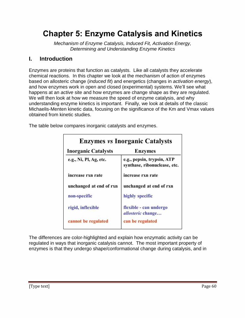
[Type text] Page 60

Chapter 5: Enzyme Catalysis and Kinetics Mechanism of Enzyme Catalysis, Induced Fit, Activation Energy,

Determining and Understanding Enzyme Kinetics

I. Introduction Enzymes are proteins that function as catalysts. Like all catalysts they accelerate chemical reactions. In this chapter we look at the mechanism of action of enzymes based on allosteric change (induced fit) and energetics (changes in activation energy), and how enzymes work in open and closed (experimental) systems. We’ll see what happens at an active site and how enzymes are change shape as they are regulated. We will then look at how we measure the speed of enzyme catalysis, and why understanding enzyme kinetics is important. Finally, we look at details of the classic Michaelis-Menten kinetic data, focusing on the significance of the Km and Vmax values obtained from kinetic studies. The table below compares inorganic catalysts and enzymes.

The differences are color-highlighted and explain how enzymatic activity can be regulated in ways that inorganic catalysis cannot. The most important property of enzymes is that they undergo shape/conformational change during catalysis, and in

[Type text] Page 61

response to cellular metabolites that indicate the biochemical status of the cell. These metabolites are often reactants (substrates) or products of other enzyme-catalyzed reactions in the same biochemical pathway as the enzyme being regulated. Voice-Over PowerPoint Presentations Catalysis VOP Enzyme Kinetics Part1 VOP Enzyme Kinetics Part2 VOP Learning Objectives

When you have mastered the information in this chapter and the associated VOPs, you should be able to: 1. compare and contrast the properties of inorganic and organic catalysts. 2. explain why catalysts do not change equilibrium concentrations of a reaction

conducted in a closed system. 3. contrast the roles of different allosteric effectors in enzymatic reactions. 4. define activation energy and compare the activation energies of catalyzed and un-

catalyzed reactions. 5. explain how an RNA molecule can function as an enzyme (ribozyme) 6. discuss how an enzyme’s active site and allosteric site interact. 7. relate enzyme kinetic equations to basic chemical rate equations. 8. distinguish between Vmax and Km in the equation for Michaelis-Menten enzyme

kinetics. 9. interpret enzyme kinetic data and the progress of an enzyme-catalyzed reaction

from this data.

II. Enzymes

Their large size and exquisite diversity of structure makes enzymes highly specific

catalysts. And because they can be deformed by interaction with other molecules, they

can be regulated. As much as catalysis itself is required to insure the efficiency of

biochemical reactions in the cell, so is this regulation. The molecular flexibility of

enzymes is required so that cells can control the rates and even the direction of

biochemical reactions and pathways. Almost no chemical reaction occurs in a that is

not directly the result of enzyme catalysis, from the digestion of nutrients in your mouth,

stomach and small intestines to pretty much every chemical reaction inside your cells.

Most enzymes are proteins, but some RNA enzymes have also been identified

(ribozymes, an example being a region of ribosomal RNA that participates in protein

synthesis) Enzymes are generally soluble in or outside cells while a few are bound to

membranes or are part of other cellular structures, but in all cases they bind to soluble

substrates.

[Type text] Page 62

The specificity of an enzyme results from the shape of the region of the molecule called

the active site, which is dependent on the 3-dimensional arrangement of amino acids in

and around the region. The active site is where reactants (called substrates) are bound

and held in place on the enzyme while rapid bond rearrangements take place. Like

many proteins, enzymes may also be bound to prosthetic groups or ions that contribute

to the shape and activity of the enzyme.

In the last few decades enzymes have been put to commercial use. For example, you

can find them in household cleaning products where they are included in detergents to

digest and remove stains caused by fats and pigmented proteins. Enzymes that break

down proteins are also added to meat tenderizers to hydrolyze proteins down to smaller

peptides.

A. The Mechanisms of Enzyme Catalysis

We describe the action of biological catalysis in two ways. One takes into account

structural features of the enzyme (active site shape, overall conformation, affinities

of the enzyme for its substrates). The other consideration involves the energetics of

enzyme action. Specifically, enzymes lower an inherent energy barrier to the

chemical reaction. This barrier is called the activation energy of the reaction. As

you may imagine, the so-called structure and energy considerations are not

unrelated.

1. Structural considerations of catalysis

From a chemistry course, you may recall that the rate of an uncatalyzed reaction

is dependent on the concentration of the reactants in solution. This is the Law of

Mass Action, recognized in then19th century. This Law makes two key

assumptions:

a) Chemical reactions eventually reach equilibrium, at which point the net rate of

formation of reaction products is zero (i.e., the forward and reverse reactions

occur at the same rate).

b) At any given time following the start of the reaction, the rate of product

formation is proportional to the concentrations of the reactants and products.

[Type text] Page 63

In practical terms, at the start of the reaction, since there are no products yet, the

reaction rate is directly proportional to the concentration of the reactants. Take a

simple reaction in which A & B are converted to B & C:

The simplified illustration of the Law of Mass Action is that at higher concentrations

of A & B there are more reactant molecules in solution and therefore a greater

likelihood that they will collide in an orientation that allows the bond rearrangements

for the reaction to occur. Of course, as products accumulate over time, reactant

concentrations decline and the rate of formation of C & D drops, now affected by

product as well as reactant concentrations.

You may recognize the chemical rate equations from a chemistry course; these

enable quantitation of reaction rates for the reaction above:

Rate of formation of products (C & D) = k1[A][B] – k-1[C][D]

This rate equation recognizes that the reaction is reversible and therefore equal to

the rate of the forward reaction (k1[A][B]) minus the rate of the reverse reaction

(k-1[C][D]). The equation is valid (applicable) at any time during the reaction.

k1 and k-1 are rate constants for the forward and reverse reactions, respectively.

So how do catalysts work? Catalysts increase chemical reaction rates by bringing

reactants together more rapidly than they would encounter each other by random

molecular motion in solution. This is possible because catalysts have an affinity for

their substrates. The attraction of reactants to inorganic catalysts is based on

relatively weak, generic attractive forces so that a metallic catalyst like silver or

platinum can attract molecules with the appropriate configurations (e.g., charge)

where they bind to the surface of catalyst just long enough to undergo a chemical

reaction.

Enzymes, unlike inorganic catalysts, have evolved highly specific shapes with

physical-chemical properties that typically attract only the substrates necessary for a

particular biochemical reaction. The active site of an enzyme thus has an affinity

for its substrate(s). The affinities of substrates for enzyme active sites are manifold

higher than for the generic surfaces of inorganic catalysts, resulting in much faster

catalysis.

A + B C + D

[Type text] Page 64

Early ideas of how substrate-enzyme interaction could be so specific involved the

Lock and Key mechanism, illustrated below.

In this model the affinity of enzyme for substrate brings them together, after which

the substrate uniquely fits into the active site like a key into a lock. Once in the

active site the substrate(s) would undergo the bond rearrangements specific for the

catalyzed reaction to generate products and regenerate an unchanged enzyme.

Subsequently the interaction of enzyme and substrate was examined using X-ray

crystallography to determine the structure of the enzyme during catalysis. These

studies revealed that upon binding to the substrate, the enzyme underwent a

conformational (i.e., allosteric) change in the active site. The result is a better fit

between enzyme and substrate.

These observations led to our understanding of the Induced Fit mechanism of

enzyme action, illustrated below.

[Type text] Page 65

2. Energetic considerations of catalysis

Catalysts work by lowering the activation energy (Ea) for a reaction, thus dramatically

increasing the rate of the reaction. Activation energy is essentially a barrier to

getting interacting substrates together to actually undergo a biochemical reaction.

Compare the random motion of substrates in solution that only occasionally

encounter one another, and even more rarely bump into one another in just the right

way to cause a reaction. This is why adding more reactants or increasing the

temperature of a reaction can speed it up (i.e., by increasing the number of random

molecular collisions). But living organisms do not have these options for conducting

fast biochemical reactions.

Inorganic catalytic surfaces can attract reactants where catalysis can then occur.

But the conformation (shape and charge configuration) of the active site of an

enzyme attracts otherwise randomly distributed substrates even more strongly,

making enzyme catalysis faster than inorganic catalysis. Again, cells do not have

the option of using inorganic catalysts because they would affect many reactions

indiscriminately… not a good way for cells to control metabolism! The advent of

enzymes with their specificity and high rate of catalysis was a key event in chemical

evolution required for the origin of life. As we saw, the initial binding of substrate to

enzyme is followed by a subtle conformational change that induces a tight fit of

substrates into the site, enabling catalysis. As a result, products of enzymatic

reactions are formed faster than those catalyzed by inorganic catalysts, and of

course much faster than the uncatalyzed reaction (millions of times faster!). The

energetics of catalysis of the simple reaction in which A & B are converted to C & D

is shown below.

[Type text] Page 66

Conducted in a closed system, enzyme-catalyzed reactions reach their equilibrium

more rapidly. As with all catalysts, enzymes are not consumed by the reactions they

catalyze, nor do they alter the equilibrium concentrations of reactants and products

of these reactions. The roughly 4000 biochemical reactions known to be catalyzed

in cells is undoubtedly an underestimate! But remember too, that we estimate that

the human genome has only 20,000 to 25,000 different genes. What do you make

of what appears to be an issue, or an inherent conflict between these two estimates?

B. Enzyme Regulation

We noted that some enzymes are regulated, which just means that factors in the cell

can slow down or speed up their rate of catalysis. In this way the cell can respond

quickly to metabolic needs reflected by the intracellular levels of these factors.

Factors that slow down catalysis are called inhibitors. Those which speed up

catalysis are called activators. In addition to responding to intracellular molecular

indicators of the biochemical status of the cell, enzymes may be inhibited by drugs,

poisons or changes in the chemical milieu (e.g. pH).

Enzymes can be regulated precisely because they are flexible and can be bent out

of shape (or into shape for that matter!). When they accumulate in cells, some small

metabolites become chemical information, signaling that they themselves are not

needed by the cell, or that the cell must accelerate other processes related to the

build-up of the metabolite.

[Type text] Page 67

Most cellular reactions occur as part of biochemical pathways, so regulating a single

enzyme can affect an entire pathway. For example, look at the pathway illustrated

below.

This generic pathway exists to produce substance E. Under normal conditions E

would be consumed in some other series of metabolic reactions. But if the cell is

meeting its metabolic needs and no longer needs so much of substance E, it will

accumulate in the cell. If there is an excess of E in the cell, some of it could bind to

any one of the enzymes in the pathway shown, inhibiting this enzyme and slowing

down the entire pathway. In this example, we can assume that allosteric regulation

of enzyme 1 evolved to control the rate of production of substance E. This is a

common mode of enzyme regulation, called feedback inhibition.

Whether an activator or an inhibitor of enzyme catalysis, regulatory molecules

typically bind to enzymes at regulatory sites (above), ultimately causing allosteric

changes in the active site. Enzyme inhibition will occur if this allosteric change

reduces the affinity of enzyme for substrate or the rate of the bond rearrangements

after the substrate has entered the active site. Activation would occur if the allosteric

effect is to increase this affinity and/or catalytic rate.

We can understand rates of enzyme catalysis and how they change when

allosterically regulated by determining enzyme kinetics. By comparing kinetic data

for each enzyme in a biochemical pathway, one can determine a standard rate-

limiting reaction under a given set of conditions. If clinical tests reveal a patient that

is producing too much or too little of an important metabolite, it might mean that a

reaction in the biochemical pathway making the metabolite that was once rate

[Type text] Page 68

limiting is not so any more. If clinical tests of a patient reveal that S/he is producing

too much of the metabolite, then the catalytic rate of the normally rate-limiting

enzyme has increased. On the other hand, if the patient is producing too little of the

metabolite, then either the catalytic rate of the rate-limiting enzyme has decreased or

the catalytic rate of another enzyme in the biochemical pathway has become rate

limiting. What might cause this phenomenon?

If levels of an important cellular molecule drop, allosteric regulation will increase

the rate of the enzyme catalyzing the rate-limiting reaction. Conversely, if an

excess of the molecule begins to accumulate in the cell, allosteric regulation can

slow down the pathway by re-establishing an appropriate rate-limiting reaction.

Viral & bacterial infection or environmental poisons can interfere with a specific

reaction in a metabolic pathway; remedies would depend on this information!

Some genetic diseases result from mutational enzyme deficiencies; prenatal

knowledge could inform the course of a pregnancy while post-natal knowledge

might dictate a course of treatment.

Treatment of a metabolic disease can itself be designed to enhance or inhibit (as

appropriate) enzyme activity.

Most enzymes are proteins. But the reaction mechanisms and kinetics of non-

protein enzymes (e.g., ribozymes and RNA components of ribosomes) can be

analyzed and classified by the same methods. We’ll look at the logic of how

enzymes are regulated in more detail when we discuss glycolysis, the anaerobic

pathway that most living things use to extract energy from nutrients.

C. Enzyme Kinetics

Common to all catalyzed chemical reactions, enzyme-catalyzed reactions display saturation kinetics, as shown below.

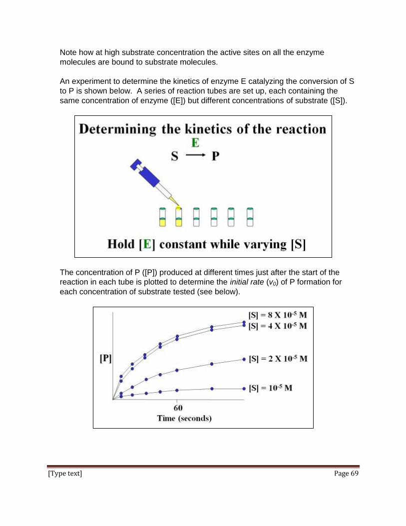
[Type text] Page 69

Note how at high substrate concentration the active sites on all the enzyme

molecules are bound to substrate molecules.

An experiment to determine the kinetics of enzyme E catalyzing the conversion of S

to P is shown below. A series of reaction tubes are set up, each containing the

same concentration of enzyme ([E]) but different concentrations of substrate ([S]).

The concentration of P ([P]) produced at different times just after the start of the

reaction in each tube is plotted to determine the initial rate (v0) of P formation for

each concentration of substrate tested (see below).

[Type text] Page 70

In this hypothetical example, the rates of the reactions (amount of P made over time)

do not increase at substrate concentrations higher than 4 X10-5 M. The upper

curves therefore represent the maximal rate of the reaction at the experimental

concentration of enzyme. We say that the maximal reaction rate occurs at

saturation.

We can estimate the initial reaction rate (vo) at each substrate concentration by

plotting the slope of the first few time points through the origin of each curve in the

graph as shown below.

Each straight (red) line is the vo for the reaction at a different [S] at the very

beginning of the reaction, when [S] is high and [P]. These rates (slopes) can be

plotted against the different concentrations of S in the experiment to get the curve

below.

[Type text] Page 71

This is an example of Michaelis-Menten kinetics common to many enzymes, named

after the two biochemists who realized that the curve described rectangular

hyperbola. Put another way, the equation mathematically describes the mechanism

of catalysis of the enzyme.

A rectangular hyperbola is mathematically described by the following equation:

You might be asked to derive, or understand the derivation of the Michaelis Menten

equation in a Biochemistry course. Suffice it to say here that Michaelis and Menten

started with some simple assumptions about how an enzyme-catalyzed reaction

would proceed and wrote reasonable chemical reactions reflecting how a catalyzed

reaction would proceed. Here are the equations for a simple reaction in which an

enzyme (E) catalyzes the conversion of substrate (S) to product (P):

Here are the reasonable chemical rate equations for this reaction that treat the

enzyme as a reactant as well as a product of the catalyzed reaction:

Next they wrote the rate equations for each of these chemical reactions, and

proceeded to re-write and combine the equations based on expectations of [S], [P],

[E], [E-S] and [E-P] at the start of the reaction.

Try writing the basic rate equations for these chemical reactions yourself!

xa

x+b y =

S P

E

E + S E-S binding of enzyme and substrate

E-S E-P conversion of substrate to product

E-P E + P dissociation of product and enzyme

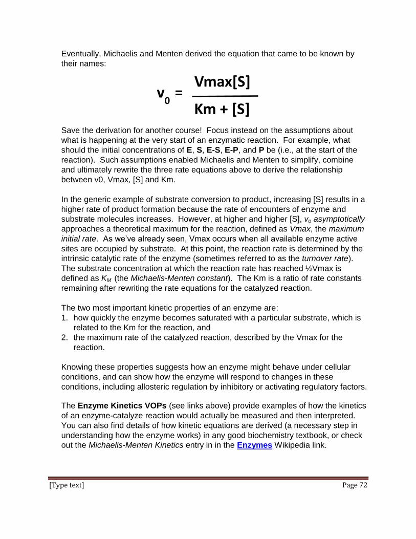
[Type text] Page 72

Eventually, Michaelis and Menten derived the equation that came to be known by

their names:

Save the derivation for another course! Focus instead on the assumptions about

what is happening at the very start of an enzymatic reaction. For example, what

should the initial concentrations of E, S, E-S, E-P, and P be (i.e., at the start of the

reaction). Such assumptions enabled Michaelis and Menten to simplify, combine

and ultimately rewrite the three rate equations above to derive the relationship

between v0, Vmax, [S] and Km.

In the generic example of substrate conversion to product, increasing [S] results in a

higher rate of product formation because the rate of encounters of enzyme and

substrate molecules increases. However, at higher and higher [S], vo asymptotically

approaches a theoretical maximum for the reaction, defined as Vmax, the maximum

initial rate. As we’ve already seen, Vmax occurs when all available enzyme active

sites are occupied by substrate. At this point, the reaction rate is determined by the

intrinsic catalytic rate of the enzyme (sometimes referred to as the turnover rate).

The substrate concentration at which the reaction rate has reached ½Vmax is

defined as KM (the Michaelis-Menten constant). The Km is a ratio of rate constants

remaining after rewriting the rate equations for the catalyzed reaction.

The two most important kinetic properties of an enzyme are:

1. how quickly the enzyme becomes saturated with a particular substrate, which is

related to the Km for the reaction, and

2. the maximum rate of the catalyzed reaction, described by the Vmax for the

reaction.

Knowing these properties suggests how an enzyme might behave under cellular

conditions, and can show how the enzyme will respond to changes in these

conditions, including allosteric regulation by inhibitory or activating regulatory factors.

The Enzyme Kinetics VOPs (see links above) provide examples of how the kinetics

of an enzyme-catalyze reaction would actually be measured and then interpreted.

You can also find details of how kinetic equations are derived (a necessary step in

understanding how the enzyme works) in any good biochemistry textbook, or check

out the Michaelis-Menten Kinetics entry in in the Enzymes Wikipedia link.

v0

=

Vmax[S]

Km + [S]

[Type text] Page 73

Some iText & VOP Key Words and Terms

activation energy enzyme Michaelis-Menten constant

active site enzyme activation Michaelis-Menten kinetics

allosteric change enzyme inhibition rate-limiting reaction

allosteric effector enzyme kinetics ribozyme

allosteric site enzyme regulation saturation kinetics

biochemical pathway induced fit substrate specificity

catalytic RNAs inorganic catalyst substrates

conformation Km Vmax

[Type text] Page 74

Chapter 6: Glycolysis, the Krebs Cycle and the

Atkins Diet Glycolysis, Gluconeogenesis & the Krebs Cycle - Getting Energy from Food;

Enzyme Regulation & the Bioenergetics of Cellular Free Energy Capture; Liver Cells in Glucose metabolism; Fooling Your Body - Atkins & South Beach Diets

I. Introduction We’ve looked at the principles governing energy flow in the universe (thermodynamics)

and in living systems (bioenergetics). We saw evidence that energy can be exchanged

between components in the universe, but it can be neither created nor destroyed. That

makes the universe a closed system, a conclusion codified as the first law of

thermodynamics. Personally, I find it a little troubling that there is no escape, until I

remind myself that the universe is a pretty big place, and I am only part of a small

system. You can define your system for yourself: the solar system, planet earth, the

country you pledge allegiance to, your city or village, your school, a farm or

homestead…)! Then derive some comfort from the realization that you can move from

one system to another and even exchange goods and services between them. This is a

metaphor for energy flow between systems in the universe.

We also said that the first law applies to closed systems within the universe. The truth

is that there are no closed systems in the universe. Systems in the universe are open,

meaning that they are always exchanging energy. What we mean by the term ‘closed

system’ is that we can define (or isolate) some small part of the universe and measure

any energy that this isolated system gives up to or takes in from its environment. The

simplest demonstration of the first law in action was using a bomb calorimeter to

measure heat released or absorbed during a chemical reaction. The second concept

we looked at was the one that says that energy flows from one place to another only

when it can. In the vernacular, we say that energy flows downhill. Anything that

happens in the universe (a galaxy moving through space, a planet rotating, you getting

out of bed, coffee perking, sugar burning in your cells, your DNA dividing) does so

because of a downhill flow of energy. We saw that by definition, any happening or

event in the universe, however large or small, is spontaneous, occurring with a release

of free energy.

With this brief reminder about energy, we are going to look at how our cells capture the

energy in nutrients. In this chapter we tackle the first two pathways of respiration to see

how we humans (and heterotrophs generally) extract the energy that was packed into

nutrients during the growth and activities of the plants and critters we eat. We’ll

compare both closed system bioenergetics for the reactions (particularly in glycolysis)

[Type text] Page 75

and then how we account for chemical reactions and energy transfer in real cells, which

are open systems that never reach equilibrium.

The manipulation of bioenergetics equations is covered in the Glycolysis VOPs. We

look at the enzymes that catalyze reactions in this evolutionarily ancient pathway, how

they are regulated, and the way in which energy is captured by several of the reactions

in the pathways . Next we’ll use the famous Atkins Diet to illustrate gluconeogenesis,

essentially a reversal of the glycolytic pathway in some cells. This pathway evolved in

animals to make glucose rather than burn it! We’ll conclude with the Krebs Cycle (also

called the TCA, or tricarboxylic acid cycle or the citric acid cycle), the second major

pathway of respiration.

The complete respiratory pathway can be summarized by the following equation:

C6H12O6 + 6O2 6CO2 + 6H2O

The standard free energy change for this reaction (Go) is about -687Kcal/mole. That

is the maximum amount of nutrient free energy that, at least in theory, could be

extracted by the complete respiration of a mole of glucose. It takes about 7.3 Kcal to

make each mole of ATP (adenosine triphosphate). Let’s see what happens in

glycolysis.

Voice-Over PowerPoint Presentations

Glycolysis Stage 1 VOP

Glycolysis Stage 2 VOP

How the Atkins Diet Works VOP

The Krebs Cycle VOP

Learning Objectives

When you have mastered the information in this chapter and the associated VOPs, you

should be able to:

1. Define (explain the difference between) glycolysis and fermentation.

2. Calculate and then compare and contrast Go and G’ for the same reaction, and

explain any differences between the change in free energy under the different

conditions.

3. Describe and explain the major events of the first and second stages of glycolysis.

4. State the role of redox reactions in glycolysis and fermentation.

5. Compare and contrast glucose (carbohydrates in general), ATP, NADH and FADH2

as high energy molecules.

[Type text] Page 76

6. Explain why only a few cell types in the human body conduct gluconeogenesis, and

articulate the purpose of this pathway.

7. Explain why the Atkins Diet works and speculate on the downside of this and the

related South Beach Diet.

8. Explain the concept of a super-catalyst and why one like the Krebs Cycle would

have evolved.

9. Compare the phosphate ester linkage in ATP and GTP and the thioester linkage in

acetyl-S-CoA and succinyl-S-CoA in terms of energetics and the reactions they

participate in.

10. Speculate on why the Krebs Cycle in E. coli generates GTP molecules and why it

generates ATP molecules eukaryotes.

II. Glycolysis (from the Greek, meaning sugar (glyco) separation (lysis), or sugar

breakdown.

One of the properties of life is that living things require energy. The pathways we look

at in this chapter are part of the flow of energy through life (shown below).

All energy on planet earth comes from the sun, via photosynthesis. Recall that light

energy fuels the formation of glucose and O2 from CO2 and water. In sum, all cells

require nutrients, using either anaerobic or aerobic processes (fermentation or

respiration) to capture nutrient free energy. The most common intracellular energy

currency is ATP. Its high energy content, derived from nutrient free energy, is readily

available to fuel almost all cellular activities. As you will see, nutrients serve to provide

energy as well as the chemical building blocks of life (amino acids, nucleic acids,

vitamins, etc.).

[Type text] Page 77

ATP is characterized as a high-energy intermediate, having captured nutrient free

energy in a form that cells can use to fuel nearly all cellular work, from building

macromolecules to bending cilia to contracting muscles to transmitting neural

information. It takes about 7.3 Kcal of free energy to make ATP in a dehydration

synthesis reaction linking a phosphate to ADP, forming a phosphate ester ‘bond’. The

hydrolysis of ATP releases that energy in reactions coupled to cellular work. The

energetics of ATP hydrolysis and synthesis are summarized below.

In animals the free energy needed to make ATP in cells comes from nutrients (sugars,

fats, proteins). Plants can capture energy from these nutrients but can also get free

energy directly from sunlight. The oxidation of a molecule of glucose releases a

considerable amount of free energy, enough to synthesize many molecules of ATP

(shown below).

[Type text] Page 78

The stepwise oxidation of glucose in cells occurs during respiration, starting with

glycolysis. Glycolysis is the first step in capturing nutrient chemical (free) energy, part

2 of the Free Energy Flow Through Life (above). It is also the oldest (most highly

conserved) biochemical pathway in evolution, found in all organisms.

The glycolytic pathway occurs in the cytosol of cells where it breaks down each

molecule of glucose (C6H12O6) into two molecules of pyruvic acid (pyruvate;

CH3COCOOH). This occurs in two stages, capturing nutrient free energy in two ATP

molecules per molecule of glucose that enters the pathway, as shown below.

In Stage 1 of glycolysis, phosphates are transferred from ATP first to glucose and then

to fructose-6-phosphate, catalyzed by hexokinase and phosphofructokinase

respectively. Free energy is consumed in Stage 1 to fuel these phosphorylations.

Next, in Stage 2, nutrient free energy is captured in ATP and NADH (reduced

nicotinamide adenine dinucleotide). In fact, four molecules of ATP and two of NADH

are produced by the time a single starting glucose molecule is split into two molecules

of pyruvic acid (pyruvate).

[Type text] Page 79

Note that NADH formation is a redox reaction; a hydrogen molecule (two protons and

two electrons) is removed from glyceraldehyde-3-phosphate and split into a proton and

a hydride ion (H-; a proton and two electrons). NAD+ is then reduced by the hydride ion.

Pyruvate is metabolized either anaerobically or aerobically. Anaerobic glycolysis

produces a net yield of two ATPs with no consumption of O2 and no net oxidation of

nutrient (i.e., glucose). Respiration is the complete oxidation of glucose to CO2 and

H2O. The anaerobic and aerobic fates of pyruvate are summarized below.

In anaerobic organisms, pyruvate is reduced by electrons in NADH, creating one of

several fermentation end-products. The most familiar, made by yeast living without

oxygen, is ethanol (alcohol). Also, if you ever experienced muscle fatigue after

especially vigorous and prolonged exercise, then you (or at least your skeletal muscles)

are guilty of fermentation, the anaerobic build-up of lactic acid in muscle cells.

In this and the next chapter we’ll focus on the oxidation of pyruvate in the Krebs cycle,

electron transport and oxidative phosphorylation, the pathways that follow glycolysis in

[Type text] Page 80

aerobes. We begin with a closer look at glycolysis, focusing on the enzyme catalyzed

reactions and watching free energy transfers between pathway components. We will

look at the energetics and enzymatic features of each reaction.

A. Glycolysis, Stage 1

Reaction 1: In the first reaction of glycolysis, glucose enters the cell and is rapidly

phosphorylated to make glucose-6-phposphate (G-6-P). This reaction is catalyzed

by the enzyme hexokinase. As shown below, the overall reaction is exergonic; the

free energy change for the reaction is -4 Kcal per mole of G-6-P synthesized.

This is a coupled reaction, meaning that the phosphorylation of glucose is coupled to

the hydrolysis of ATP. In energy terms, the free energy of ATP hydrolysis

(energetically favorable) is used to fuel the phosphorylation of glucose (energetically

unfavorable). The reaction is also biologically irreversible, as shown by the single

vertical arrow above.

Excess dietary glucose is stored in most cells, but especially liver and kidney cells,

as glycogen, a highly branched polymer of glucose monomers. Glucose made by

photosynthesis in green algae and plants stored as starch. In animals glycogen is

hydrolyzed back to glucose in the form of glucose-1-phosphate (G-1-P) which is

converted to G-6-P.

[Type text] Page 81

Let’s take a look at the energetics (free energy flow) for the coupled hexokinase-

catalyzed reaction. This reaction is actually the sum of the two coupled reactions, as

shown below.

As you can see, ~7 Kcal/mole (rounding down!) are released by ATP hydrolysis in a

closed system under standard conditions, an exergonic reaction. On the other hand,

the dehydration synthesis reaction of glucose phosphorylation occurs with a G0 of

+3 Kcal/mole. This is an endergonic reaction under standard conditions. Summing

up the free energy changes of the two reactions, we get the overall G0 of -4

Kcal/mole for the coupled reaction under standard conditions in a closed system.

Recall that all chemical reactions are inherently reversible (see Enzyme Catalysis

and Kinetics). But we noted that the overall coupled reaction is biologically

irreversible. We say an enzyme catalyzed reaction is biologically irreversible when

the products have a relatively low affinity for the enzyme active site, making catalysis

of the reverse reaction very inefficient. As you will see, biologically irreversible

reactions, including the phosphorylation of glucose catalyzed by hexokinase, are

often regulated. Hexokinase is allosterically regulated by G-6-P.

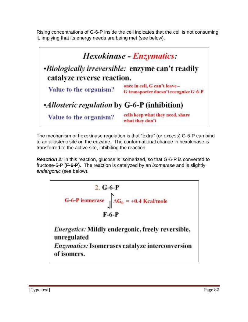
[Type text] Page 82

Rising concentrations of G-6-P inside the cell indicates that the cell is not consuming

it, implying that its energy needs are being met (see below).

The mechanism of hexokinase regulation is that “extra” (or excess) G-6-P can bind

to an allosteric site on the enzyme. The conformational change in hexokinase is

transferred to the active site, inhibiting the reaction.

Reaction 2: In this reaction, glucose is isomerized, so that G-6-P is converted to

fructose-6-P (F-6-P). The reaction is catalyzed by an isomerase and is slightly

endergonic (see below).

[Type text] Page 83

Reaction 3: In this reaction, the enzyme 6-phosphofruktokinase catalyzes the

phosphorylation of F-6-P to make fructose 1, 6 di-phosphate (F1,6 diP). This is also

a coupled reaction, with ATP providing this second phosphate. The overall reaction

and the separation of the two coupled reactions are shown below.

As for the hexokinase reaction, the 6-P-fructokinase reaction is exergonic and

biologically irreversible. Phosphofructokinase is also allosterically regulated, in this

case by several different allosteric effectors, including ATP, ADP and AMP and long-

chain fatty acids.

Reactions 4 and 5: These are the last reactions of the first stage of glycolysis. In

one reaction, F1,6 diP (6-carbon sugar) is reversibly split into dihydroxyacetone

phosphate (DHAP) and glyceraldehude-3-phposphate (G-3-P). In the second

reaction (also reversible) the DHAP is converted into G-3-P. Here are the reactions:

[Type text] Page 84

The net result is the formation of 2 molecules of G-3-P. The enzymes F-diP

aldolase and triose-P-isomerase both catalyze freely reversible reactions. Also, both

reactions proceed with a positive free energy change and are therefore endergonic.

The sum of the free energy changes for the splitting of F1,6 diP into two G-3-Ps is a

whopping +7.5 Kcal per mole, a very energetically unfavorable process.

Summing up, by the end of stage 1 of glycolysis, we have consumed 2 ATP

molecules, and split one 6C carbohydrate into two 3C carbohydrates. We have also

seen two biologically irreversible and allosterically regulated enzymes.

B. Glycolysis, Stage 2

Stage 1 of glycolysis ends with the splitting of a 6-carbon sugar (glucose) into two 3-

carbon carbohydrates (G-3-P). We’ll follow just one of these G-3-P molecules, but

remember that both are proceeding through Stage 2 of glycolysis.

Reaction 6: This is the redox reaction we promised earlier, in which G-3-P is

oxidized and NAD+ is reduced. As shown below, the enzyme glyceraldehyde-3-

phopsphate dehydrogenase also catalyzes the phosphorylation of a phosphoglyceric

acid intermediate to make 1,3, diphosphoglyceric acid (1,3, diPG).

In this freely reversible endergonic reaction, a hydrogen molecule (H2) is removed

from G-3-P in the form of a hydride ion (H-) and a proton (H+). NAD+ is reduced by

the H- ion, leaving behind the protons in solution.

[Type text] Page 85

G-3-P dehydrogenase is regulated by levels of one of its substrates, NAD+.

Regulation is by a form of allosteric regulation called negative cooperativity: the

higher the [NAD+] , the lower the affinity of the enzyme for more NAD+ and the faster

the reaction in the cell!

Reaction 7: The reaction shown below, catalyzed by the enzyme phosphoglycerate

kinase, is freely reversible and exergonic, yielding ATP and 3-phosphoglyceric acid

(3PG).

Kinases are enzymes that transfer phosphate groups between molecules, most

often to ADP to make ATP by what is called substrate-level phosphorylation. In

this coupled reaction the free energy released by hydrolyzing a phosphate from 1,3

diPG is used to make ATP. Remember that this reaction occurs twice per starting

glucose, so that at this point in glycolysis, two ATPs have been synthesized.

Reaction 8: This freely reversible endergonic reaction moves the phosphate from

the number 3 carbon of 3PG to the number 2 carbon as shown below.

Mutases like phoshoglycerate mutase are enzymes that catalyze the transfer of

functional groups within a molecule.

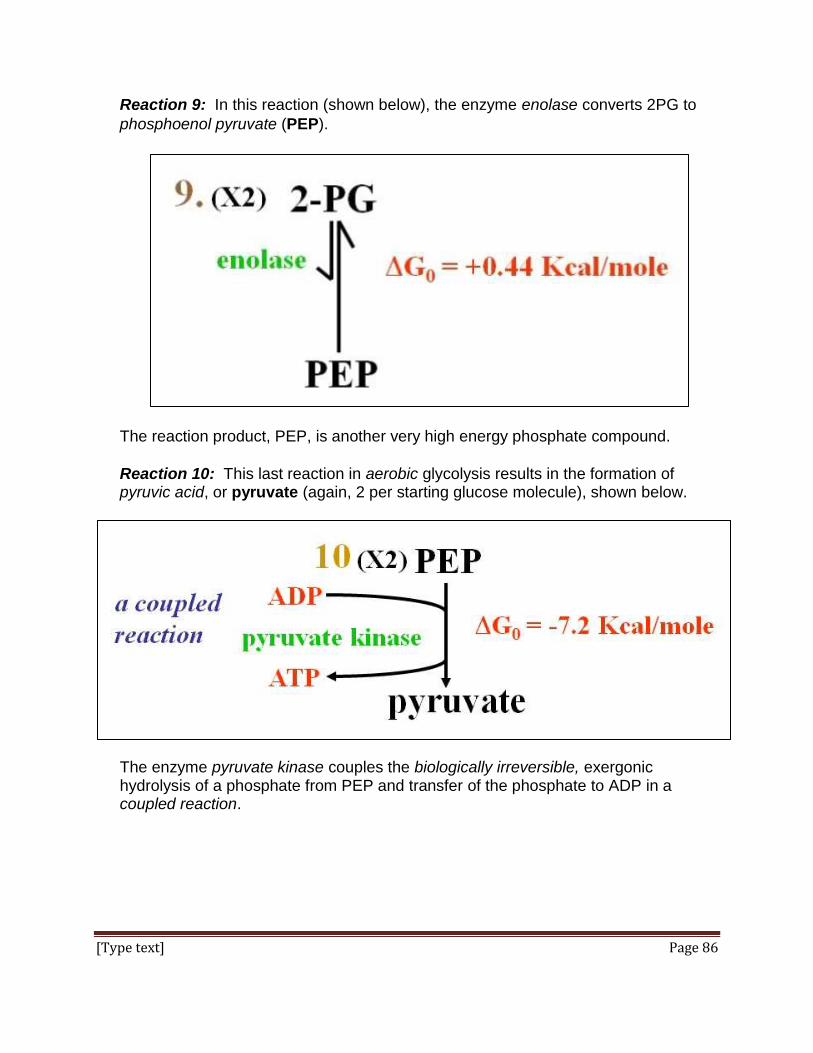
[Type text] Page 86

Reaction 9: In this reaction (shown below), the enzyme enolase converts 2PG to

phosphoenol pyruvate (PEP).

The reaction product, PEP, is another very high energy phosphate compound.

Reaction 10: This last reaction in aerobic glycolysis results in the formation of pyruvic acid, or pyruvate (again, 2 per starting glucose molecule), shown below.

The enzyme pyruvate kinase couples the biologically irreversible, exergonic hydrolysis of a phosphate from PEP and transfer of the phosphate to ADP in a coupled reaction.

[Type text] Page 87

Aerobic glycolysis is sometimes called incomplete glycolysis. If pyruvate is reduced

in subsequent reactions the pathway becomes complete glycolysis, also called a

fermentation (see the Alternate Fates of Pyruvate, above). Pyruvate kinase is

allosterically regulated by ATP, citric acid, long-chain fatty acids, F1,6 diP, and one

of its own substrates, PEP.

Here is a balance sheet for both complete and incomplete glycolysis, showing

chemical products and energy transfers.

There are 2 reactions in Stage 2 of glycolysis that each yields a molecule of ATP.

Since each of these reactions occurs twice per starting glucose molecule, the 2nd

stage of glycolysis produces 4 ATP molecules. Since 2 ATPs were consumed in

stage 1, the net yield of chemical energy as ATP by the end of glycolysis down to

pyruvate is 2 ATPs. That’s just about 15 Kcal conserved as the chemical energy of

ATP… out of 687 Kcal potentially available from the mole of glucose! As you will

see, there is a lot more free energy available from glucose, much of which remains

to be captured during the rest of respiration.

On the other hand, anaerobes which can’t make use of oxygen, usually have to

settle for the paltry 15 Kcal they get in the net yield of 2 moles of ATP per starting

mole of glucose.

[Type text] Page 88

Remember that one of the reactions in the 2nd stage of glycolysis is actually a

chemical oxidation. But check out fermentation pathways: you will find that there is

no net oxidation of glucose (i.e., glycolytic intermediates) by the end of a

fermentative pathway.

By this time, you will have realized that glycolysis is an energetically favorable

(downhill) reaction in a closed system, with an overall negative Go. In most of our

cells glycolysis is normally spontaneous, driven by a constant need for energy to do

cellular work. Thus the actual free energy of glycolysis, or G’, is also negative.

So next we’ll look at gluconeogenesis, the Atkins Diet and some not-so-normal

circumstances when glycolysis essentially goes in reverse, at least in a few cell

types. Under these conditions, glycolysis is energetically unfavorable, and those

reverse reactions are the ones proceeding with a negative G’!

III. Gluconeogenesis

In a well-fed animal, most cells can store a small amount of glucose as glycogen. All

cells break glycogen down as needed to retrieve nutrient energy as G-6-P. Glycogen

hydrolysis is called glycogenolysis. For most cells, glycogen is quickly used up between

meals. Therefore these cells depend on an external source of glucose other than diet.

Those sources are liver and to a lesser extent, kidney cells, which can store large

amounts of glycogen after meals. In continual feeders (for examples cows and other

ruminants), glycogenolysis is ongoing. In intermittent feeders (like us) liver

glycogenolysis can supply glucose to the blood for distribution to all cells of the body for

6-8 hours between meals, depending on the level of activity. So, after a good night’s

sleep, a period of intense exercise, a day or any prolonged period of low carbohydrate

intake (fasting or starvation), even liver and kidney glycogen reserves will be mobilized

and even depleted. Under these circumstances, animals use gluconeogenesis

(literally, new glucose synthesis) in liver and kidney cells to provide systemic glucose to

nourish other cells. As always in otherwise healthy individuals, the hormones insulin

and glucagon regulate blood glucose homeostasis, protecting against hypoglycemia

(low blood sugar) and hyperglycemia (high blood sugar) respectively.

Gluconeogenesis is a metabolic pathway that produces glucose from non-carbohydrate

carbon substrates. In humans these substrates include pyruvate, lactate, glycerol and

gluconeogenic amino acids (those that can be converted to alanine). Except for so-

called bypass reactions, gluconeogenesis is essentially a reversal of glycolysis. The

bypass reactions are necessary to get around the three biologically irreversible

reactions of glycolysis.

[Type text] Page 89

The pathways of glycolysis and gluconeogenesis are illustrated side by side (below) to

highlight both the bypass reactions and those of glycolysis that function in

gluconeogenesis.

If glycolysis is an exergonic pathway, then gluconeogenesis must be an endergonic

one. Gluconeogenesis is only possible if the bypass enzymes arte present. Not shown

in the pathway is the fact that gluconeogenesis consumes 4 ATP and 2 GTP molecules.

But In spite of this free energy requirement, gluconeogenesis is energetically favorable!

[Type text] Page 90

This is because the cell is an open system. An accumulation of pyruvate and the rapid

release of new glucose from the cells into the blood drive the reactions toward glucose

synthesis. And pyruvate will build up if the liver (or kidney) cells experience a buildup of

gluconeogenic amino acids.

As implied in the foregoing discussion, glycolysis and gluconeogenesis are not

simultaneous! As in all cell types, glycolysis is the normal pathway. Gluconeogenesis

in liver (and kidneys) is regulated by glucocorticoid hormones that signal the cells to

synthesize the bypass reaction enzymes (the two carboxylases and phosphatases

indicated in brown in the illustration).

The same glucocorticoid hormones also stimulate other cell types to break down fats

and proteins (below).

Levels of lipases that catalyze fat hydrolysis increase in response to glucocorticoids,

generating fatty acids and glycerol. Most cells can use fatty acids as an alternate

energy nutrient when glucose is limiting. Glycerol is then taken up by liver cells and

converted to G-3-P, contributing to gluconeogenesis. In skeletal muscle,

hypothalamic-

pituitary

axis

[Type text] Page 91

glucocorticoids stimulate the synthesis of proteolytic enzymes that catalyze protein

breakdown to amino acids that enter the circulation. Gluconeogenic amino acids

reaching the liver and kidneys are converted to pyruvate, also contributing to

gluconeogenesis.

A long night’s sleep, fasting and more extremely, starvation are a form of stress. Our

stress response begins in the hypothalamic-pituitary axis. A consequence is that the

hypothalamus secretes a neurohormone that stimulates the release of ACTH

(adrenocorticotropic hormone) from the pituitary gland. ACTH then stimulates the

release of cortisone and similar glucocorticoids from the cortex (outer layer) of the

adrenal glands . As the name glucocorticoid suggests, these hormones participate in

the regulation of glucose metabolism. At times when carbohydrate intake is low, the

organism reacts by mobilizing alternative energy sources and by making carbohydrates

(i.e., glucose) from non-carbohydrate sources. Here are the details:

Glucocorticoids stimulate gluconeogenic bypass enzyme synthesis in liver cells.

Glucocorticoids stimulate skeletal muscle protease synthesis in skeletal muscle

causing hydrolysis of the peptide bonds between amino acids. Gluconeogenic

amino acids circulate to the liver where they are the most abundant substrate for

gluconeogenesis. Ketogenic amino acids resulting from proteolysis are not used in

gluconeogenesis. When they are used as substrates for ketogenesis during

prolonged fasting, ketosis may occur, characterized by pungent “acetone” breath in

undernourished or starving patients.

The heart and brain require glucose for energy, and cannot use fats as an

alternative. Thus, the essential role of gluconeogenesis is to supply glucose to

these organs in the absence of adequate carbohydrate in the diet, including during

fasting or starvation. Glucocorticoids induced lipases catalyze hydrolysis of the

ester linkages between fatty acids and glycerol in fats (triglycerides) in most cells,

including adipose tissue, a major storehouse of fats. As we noted, fatty acids are an

alternate energy source to carbohydrates for most cells, and glycerol will circulate to

the liver where it is converted to G-3-P to serve not as a glycolytic intermediate, but

as a gluconeogenic substrate!.

It’s a pity that we humans cannot use fatty acids as gluconeogenic substrates! Plants

and some lower animals have a glyoxalate cycle pathway that can convert the product

of fatty acid oxidation (acetate) directly into carbohydrates that can enter the

gluconeogenic pathway. But we and higher animals in general lack this pathway. Thus,

we cannot convert fats to carbohydrates, in spite of the fact that we can all too easily

convert the latter to the former!

[Type text] Page 92

IV. The Atkins Diet and Gluconeogenesis

You may know that The Atkins Diet is an ultra-low carb diet. On this diet a person is in

a pretty much constant gluconeogenic state. While the liver can produce enough

glucose for brain and heart cells, the rest of the cells in our bodies will switch to burning

fats, hence the weight loss. Discredited a few years back, the Atkins Diet and similar

ones like the South Beach diet are now back in favor. On a low glucose (low carb) diet

like the Atkins diet, glucocorticoids are released, tricking the body into a gluconeogenic

state. While heart and brain get their glucose, other cells switch to fats as an alternate

source of energy by turning on the synthesis of required enzymes. Hence the weight

loss…

V. The Krebs/TCA/Citric acid cycle

In a well fed organism dietary glucose can fulfill the energy needs of all cells. Pyruvate

from glycolysis will enter mitochondria to be oxidized to Acetyl-S-Coenzyme A

(Ac-S-CoA), which will then be oxidized in the Krebs cycle. The products of complete

oxidation of each pyruvate molecule include and 3CO2 and an ATP molecule, along with

a lot of reduced electron carriers. These molecules (NADH, FADH2) have captured

most of the free energy in the original glucose molecules. These reactions are

summarized below.

[Type text] Page 93

The enzyme pyruvate dehydrogenase catalyzes the oxidation of pyruvate, converting a

3-carbon carbohydrate into acetate, a 2-carbon molecule, acetate, releasing a molecule

of CO2. In this highly exergonic reaction CoA-SH forms a high energy thioester linkage

with the acetate in Ac-S-CoA:

The Krebs cycle is a cyclic pathway whose key functions are to oxidize Ac-S-CoA,

reduce NAD+ to NADH, and provide intermediates that can be converted into some

amino acids. The Krebs Cycle we see in humans today is shared by all aerobic

organisms, indicating that that it arose early in the evolution of our oxygen environment.

Because of the role of Krebs Cycle intermediates in other biochemical pathways, parts

of the pathway may have pre-dated the complete respiratory pathway. The Krebs Cycle

takes place in mitochondria of eukaryotic cells. It is also called the citric acid cycle and

the tricarboxylic acid cycle because its first reaction product, citric acid, contains 3

carboxyl groups! The Krebs Cycle as it occurs in animals is summarized below.

[Type text] Page 94

This is a pretty busy image. It begins a series of step-wise reactions with the oxidation

of the 3-carbon pyruvate molecule, generating a of 2-carbon acetate (Ac-S-CoA)

molecule and a molecule of CO2. In the cycle:

find the 2 molecules of CO2 produced in the Krebs Cycle itself.

find GTP (which quickly transfers its phosphate to ADP to make ATP). In bacteria,

ATP is made directly at this step.

count all of the reduced electron carriers (NADH, FADH2). Each of the latter carries

a pair of electrons, so including those on the each of the NADH molecules made in

glycolysis, how many electrons have been removed from glucose during its

oxidation?

Remember that two pyruvates are produced per glucose; so for each glucose, two

molecules of Ac-S-CoA are produced and the cycle turns twice!

Each NADH carries about 50 Kcal of the 687 Kcal of free energy originally available in a mole of glucose; each FADH2 carries about 45 Kcal of this free energy. This energy will fuel ATP production during electron transport and oxidative phosphorylation. The high energy thioester bonds formed in this pathway fuel ATP synthesis as well as the condensation of oxaloacetate and acetate in the first reaction.

Finally, the story of how we come to understand the Krebs cycle is almost as interesting

as the cycle itself! In 1937, Albert Szent-Györgyi won a Nobel Prize for discovering a

few of the reactions of the cycle, which he and everyone else believed were part of a

linear pathway. In that same year, Hans Krebs performed a series of elegant

experiments that revealed these crucial respiratory reactions to be part of a cyclic

pathway. Krebs won the Nobel Prize for this work in 1953!

Some iText & VOP Key Words and Terms

Acetyl-S-coenzyme A (Ac-S-CoA)

free energy capture oxidizing agent

ADP, ATP, GDP, GTP fructose phosphatase enzymes

aerobic G, G6P, F6P, F1,6-diP phosphate-ester linkage

anaerobic gluconeogenesis redox reactions

Atkins Diet gluconeogenic amino acids reducing agent

biochemical pathways glycolysis respiration

[Type text] Page 95

bioenergetics glyoxalate cycle SDH (succinate dehydrogenase)

bypass reactions, enzymes high energy bond (linkage) spontaneous reaction

C6H12O6 (glucose) high energy molecules stage 1

cells as open systems isomerase enzymes stage 2

dehydrogenase enzymes kinase enzymes standard conditions

DHAP, G3P,1,3-diPG, 3PG, 2PG, PEP, Pry

Krebs (TCA, citric acid) cycle

steady state

diabetes metabolic effects of low carb diet

stoichiometry of glycolysis

energetics of glycolysis metformin substrate level phosphorylation

energy flow in cells mitochondria Succinyl-S-CoA

equilibrium mutase enzymes super-catalyst

FAD (oxidized nicotinamide adenine di-Phosphate)

NAD+ (oxidized nicotinamide adenine di-Phosphate)

synthase enzymes

FADH2 (reduced flaming adenine di-Phosphate)

NADH (reduced nicotinamide adenine di-Phosphate)

thioester linkage

fermentation nutrients G’ (actual free energy change)

free energy oxidation, reduction Go (standard free energy change)

[Type text] Page 96

Chapter 7: Electron Transport, Oxidative

Phosphorylation, Photosynthesis Electron Transport and Oxidative Phosphorylation; oxidizing NADH and FADH2; Chemiosmosis Mechanism and Protein Motors Make ATP; Photosynthesis as a

precursor to respiration; Reducing CO2 with electrons from H2O; Light-dependent and Light-independent reactions

I. Introduction

We have seen that glycolysis generates 2 pyruvate molecules per glucose molecule,

and that each is then oxidized to 2 Ac-S-CoA molecules. Then after each Ac-S-CoA

has been oxidized by the Krebs cycle, aerobic cells have on a molar basis, captured

about 30 Kcal out of the 687 Kcal potentially available from glucose. Not much for all

the biochemical effort! But a total of 24 H+ (protons) pulled from glucose in redox

reactions have also been captured, in the form or the reduced electron carriers NADH

and FADH2. In this chapter we look at electron transport and oxidative phosphorylation,

the linked (“coupled”) mechanism whereby a significant part of the remaining free

energy that was once in a mole of glucose ends up in ATP. We shall see that the flow

of electrons during the oxidation of electron carriers during electron transport releases

free energy that is first captured as an H+, or proton gradient. In turn, oxidative

phosphorylation uses the energy released as the gradient dissipates to fuel ATP

synthesis. We will note that the mechanism of oxidative phosphorylation is quite

different than the substrate-level phosphorylation that describes ATP synthesis in

glycolysis and the Krebs Cycle. We’ll conclude our consideration of respiration with an

energy balance sheet for respiration and summary of how free energy is captured from

alternate nutrients. Finally, we’ll provide some details of photosynthesis, which is

basically the opposite of respiration, and compare similar aspects of the photosynthetic

and respiratory pathways.

Voice-Over PowerPoint Presentations

Electron Transport VOP

Oxidative Phosphorylation VOP)

Learning Objectives

When you have mastered the information in this chapter and the associated VOPs, you

should be able to:

1. explain the centrality of the Krebs Cycle to aerobic metabolism.

2. identify the sources of electrons in redox reactions leading up to and within the

Krebs cycle.

[Type text] Page 97

3. illustrate the paths of electrons from the Krebs cycle to and through the electron

transport chain.

4. trace the evolution of the electron transport chain from its location on an aerobic

bacterial membrane to its location in eukaryotic cells.

5. distinguish between a proton gate and a proton pump.

6. interpret experiments involving redox reactions, ATP synthesis and ATP hydrolysis

conducted with intact mitochondria and separated mitochondrial membranes.

7. interpret pH changes in and surrounding mitochondria resulting from such

experiments.

8. distinguish between the component pH, H+ and electrical gradients established

during electron transport and dissipated during oxidative phosphorylation.

9. explain the chemiosmotic mechanism of ATP synthesis and contrast it with

substrate-level phosphorylation.

10. Compare and contrast the role of electron transport in respiration and

photosynthesis and discuss the evolution of each.

11. Trace the paths of electrons taken in photosynthesis and explain each path.

12. explain the presence of similar biochemical intermediates min respiration and

photosynthesis

II. The Electron Transport Chain

All cells use electron transport chains to oxidize substrates in free energy-releasing

(exergonic, spontaneous) reactions. The respiratory ETC oxidizes the reduced electron

carriers produced in glycolysis and the Krebs Cycle (NADH, FADH2), while an ETC in

plants and other photosynthetic organisms serves to oxidize NADPH (a phosphorylated

version of the electron carrier NADH). In both cases, free energy released during the

redox reactions of an ETC fuels the transport of protons (H+ ions) across a membrane,

creating a proton gradient that is at once an electrical and a chemical gradient. This

electrochemical gradient contains the free energy originally in the reduced substrates.

This free energy released when protons are allowed to flow (diffuse) back across the

membrane. This proton diffusion is coupled to ATP production. The energizing an

electrochemical gradient and capturing the gradient free energy as ATP is called the

Chemiosmotic Mechanism. In aerobic respiration, electrons are ultimately transferred

from components at the end of the ETC to molecular oxygen (O2), making water. In

photosynthesis, electron transfer reduces CO2 to sugars.

Here we focus on the details of respiration as it occurs in the mitochondria of eukaryotic

cells. The end products of electron transport are NAD+, FAD, water and protons, which

are pumped across the cristal membrane of mitochondria to create the proton gradient.

In the illustration below, roman numbered protein complexes along with Coenzyme Q

[Type text] Page 98

(just Q in the drawing) and cytochrome C (Cyt c) are participants in a sequence of

reactions in which electrons acquired by oxidizing NADH or FADH2 to NAD+ and FAD

(respectively) are transferred from one complex to the next, until electrons, protons and

oxygen unite to in complex IV to make water. Under standard conditions in a closed

system, electron transport is downhill, with an overall release of free energy (negative

Go) at equilibrium.

From the illustration above, we can see three sites in the respiratory ETC which function

as H+ pumps. That is, they are sites where the negative change in free energy of

electron transfer is large, and coupled to the action of a proton pump. The result is that

protons accumulate outside the matrix of the mitochondrion. Because the outer

mitochondrial membrane is freely permeable to protons, the electrochemical gradient is

in effect between the cytoplasm and the mitochondrial matrix. When the gradient is

relieved by allowing the protons to flow back into the mitochondrial matrix, free energy

of the gradient is released and harnessed as chemical energy.

[Type text] Page 99

III. Oxidative Phosphorylation

Free energy in mitochondrial proton gradient is captured as ATP by Oxidative

phosphorylation. Most of the ATP made in aerobic organisms is made by oxidative

phosphorylation, rather than by substrate phosphorylation (the mechanism of ATP

synthesis in glycolysis or the Krebs Cycle). In fact, aerobic respiratory pathways

evolved in an increasingly oxygenic environment because its pathways were more

efficient at making ATP than fermentations such as ‘complete’ glycolysis.

Recall that ATP synthesis from ADP and inorganic phosphate is endergonic under

standard conditions in a closed system. In substrate-level phosphorylation, the

hydrolysis of very high energy nutrient intermediates of glycolysis or the Krebs Cycle is

coupled to ATP synthesis. In oxidative phosphorylation, the controlled diffusion of

protons across the cristal membrane into the mitochondrial matrix is coupled to ATP

synthesis on a complex of proteins and enzymes called an ATP synthase.

As we have seen, the movement of electrons down the electron transport chain fuels 3

proton pumps that establish a proton gradient across the cristal membrane. Free

energy is stored in this (in fact in any) gradient. Oxidative phosphorylation is the system

that evolved to couple proton flow into the mitochondrial matrix to the capture of proton

gradient-free energy. Because protons carry a positive charge, the gradient produced is

also an electrochemical one. We say that the proton gradient has a proton-motive

force. It has two components: a difference in proton concentration (a H+ gradient, or

ΔpH) and a difference in electric potential. The latter is similar to the stored energy in a

common battery. When the battery is in an appliance (flashlight, cell phone, etc.),

turning it on with a switch is like poking holes in the cristal membrane. The switch in the

mitochondrial cristal membrane is the ATP synthase protein complex. The capture of

free energy of protons flowing through the complex is summarized below.

[Type text] Page 100

In mitochondria, the protons that are pumped out of the mitochondrial matrix using the free energy released by electron transport can flow back into the matrix through the ATP synthase. If there are 3 ETC proton pumps in the cristal membrane, then the cristal membrane ATPase complexes function as proton gates that catalyzes ATP synthesis from ADP and inorganic phosphate when protons are allowed to flow through them. But, proton flow through the gates is regulated.

When ATP is high (meaning that the cells energy needs are being met), the gate is

closed and the proton gradient cannot be relieved. But if ADP levels are relatively high

(a signal that the cell is hydrolyzing a lot of ATP… and needs more), the gate will open.

As protons move through the gate (by diffusion), they power a molecular (protein) motor

in the ATP synthase that in turn, activates ATP synthesis.

A very similar electron transport chain exists in the cell membrane of bacterial, which of

course lack mitochondria, but which according to the endosymbiotic theory, are the

ancestors of mitochondria. The chemiosmotic mechanism of ATP generation in aerobic

bacteria is therefore much the same as in eukaryotic mitochondria.

Proton gradients not only power ATP synthesis, but in some cases, can power cellular

activities more directly. The best example of this is the bacterial flagellum that is

directly attached to the molecular motor of a proton gate protein complex in the cell

membrane (below).

Electron transport in the cell membrane creates the gradient, and relief of the gradient

directly powers the flagellum.

From: H+ ions fuel a bacterial flagellar motor

[Type text] Page 101

IV. Photosynthesis

Chemically, photosynthesis is the reverse reaction of respiration. Compare the two

reactions:

1. C6H12O6 + 6O2 6CO2 + 6H2O (Go = -687Kcal/mole)

2. 6CO2 + 6H2O C6H12O6 + 6O2 (Go = +687Kcal/mole)

If respiration (reaction 1) is the complete oxidation of glucose to H2O and CO2, then

photosynthesis (reaction 2) is the reduction of CO2 using electrons from H2O.

Photosynthesis is an endergonic pathway; sunlight (specifically visible light, fuels the

reduction of CO2 (summarized below).

The evolution of photosynthesis could only have occurred before the advent of

respiration, since it is photosynthesis that began generating the molecular oxygen that

characterizes our atmosphere today. If we look at photosynthesis in some detail, we

will see an electron transport system that pumped protons and coupled gradient free

energy to ATP synthesis, one that evolved before the respiratory pathways, and that

might have been the source of respiratory pathway reactions in evolution later in

evolution.

[Type text] Page 102

Photosynthesis is basically two pathways:

Light-dependent reactions that use visible light energy to remove electrons from

water and reduce electron carriers, and to make ATP;

Light-independent reactions that use ATP to transfer electrons from the reduced

electron carriers to CO2 to synthesize glucose.

The two pathways are summarized below.

A. The Light Dependent Reactions

An early experiment (below) established that only wavelengths of visible light energy

functioned in photosynthesis, and that in fact, most wavelengths (colors) of light

would stimulate photosynthesis in plants.

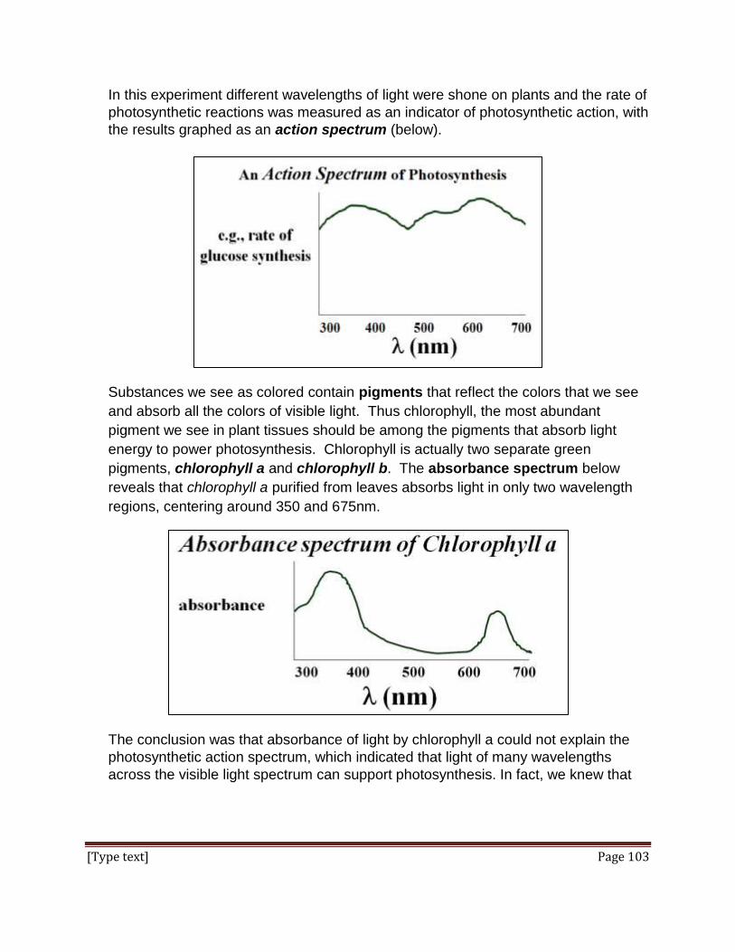
[Type text] Page 103

In this experiment different wavelengths of light were shone on plants and the rate of

photosynthetic reactions was measured as an indicator of photosynthetic action, with

the results graphed as an action spectrum (below).

Substances we see as colored contain pigments that reflect the colors that we see

and absorb all the colors of visible light. Thus chlorophyll, the most abundant

pigment we see in plant tissues should be among the pigments that absorb light

energy to power photosynthesis. Chlorophyll is actually two separate green

pigments, chlorophyll a and chlorophyll b. The absorbance spectrum below

reveals that chlorophyll a purified from leaves absorbs light in only two wavelength

regions, centering around 350 and 675nm.

The conclusion was that absorbance of light by chlorophyll a could not explain the

photosynthetic action spectrum, which indicated that light of many wavelengths

across the visible light spectrum can support photosynthesis. In fact, we knew that

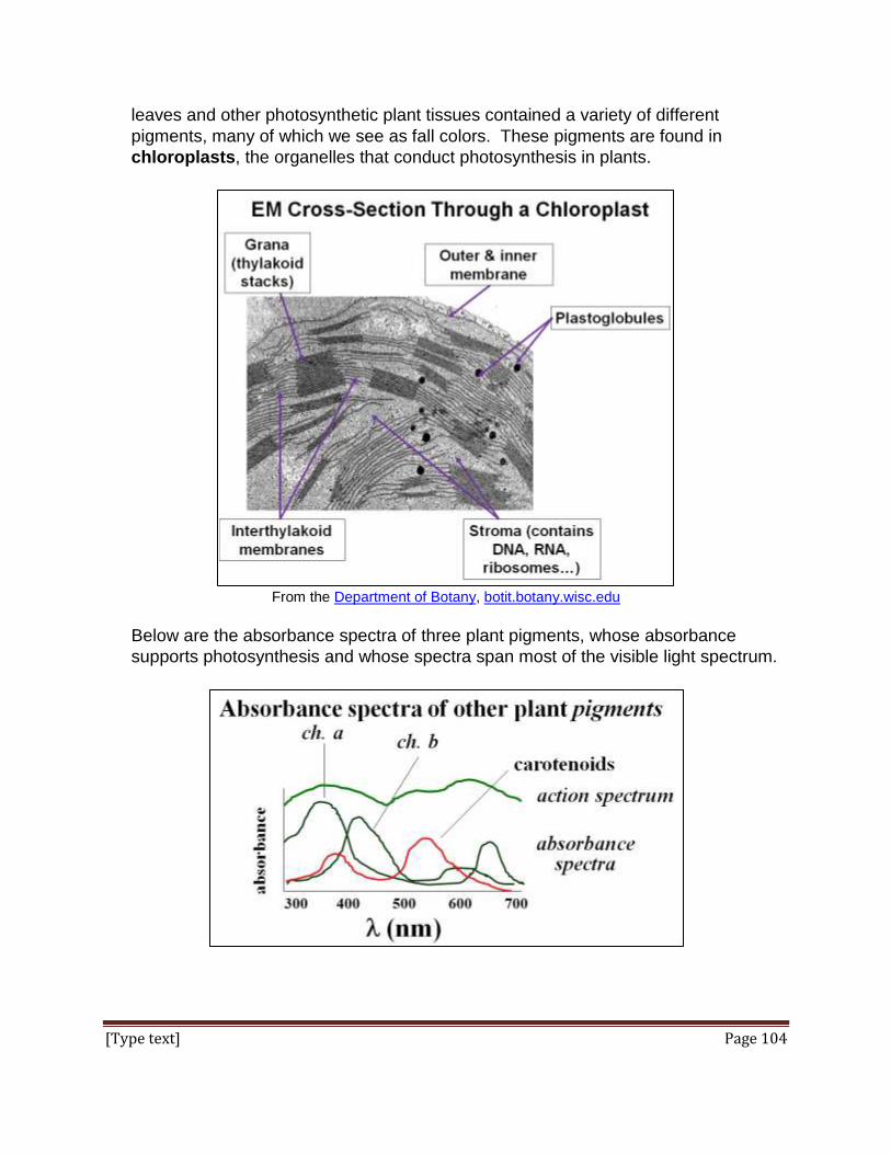
[Type text] Page 104

leaves and other photosynthetic plant tissues contained a variety of different

pigments, many of which we see as fall colors. These pigments are found in

chloroplasts, the organelles that conduct photosynthesis in plants.

From the Department of Botany, botit.botany.wisc.edu

Below are the absorbance spectra of three plant pigments, whose absorbance

supports photosynthesis and whose spectra span most of the visible light spectrum.

[Type text] Page 105

Carotenoids, chlorophyll b and other accessory pigments participate in capturing

light energy for photosynthesis. These pigments are organized into two

photosystems on thylakoid membranes of chloroplasts. The activities of

Photosystem I are animated in this link: http://youtu.be/BLEB0A_9Tt4. You should

see light (a photon) excite electron (e-) pairs excited from Photosystem I pigments

that then transfer their energy from pigment to pigment, ultimately to chlorophyll a

P700, from which an e-pair is excited and captured by a photosystem I (PSI) e-

acceptor. The reduced PSI acceptor is then oxidized with its electrons transported

along a short ETC, eventually reducing NADP+ to NADPH. Electrons on NADPH

will eventually be used to reduce CO2 to a carbohydrate. So far, so good! But that

leaves an e- deficit in Photosystem I. The Z-Scheme illustrated below follows

electrons as they are taken from water (absorbed through roots) and used to replace

those missing from PSI.

After electrons from PSI reduce NADP+ to NADPH, they are replaced with electrons

excited by light from PS2. The electrons excited in PSII are ultimately excited from

the P680 form of chlorophyll a, and are captured by a PSII electron acceptor in the

thylakoid membrane, which has been identified as pheophytin. When pheophytin is

oxidized, its electrons move to PSI down an ETC in the thylakoid membrane. Some

of the free energy released by electron transport is used to pump protons from the

[Type text] Page 106

stroma into the space surrounded by the thylakoid membranes. When the protons

are allowed to flow back into the stroma, the gradient free energy is coupled to ATP

synthesis by a chloroplast ATP synthase. The link at http://youtu.be/t4RlsDDsNi8

animates the entire Z-Scheme, showing first how PSI electrons reduce NADP+ and

then how PSII electrons replace missing PSI electrons, making ATP along the way.

The oxygen released by splitting water ends up in the atmosphere.

B. Cyclic Photophosphorylation

The Z-Scheme does not in fact make enough ATP to power the Calvin Cycle. But

when the need for ATP exceeds the capacity of the tissues to make sugar, the

photosynthetic apparatus can take a time-out, resorting to Cyclic Photo-

phosphorylation for a while.

Cyclic Photophosphorylation simply takes electrons excited to the PSI electron

acceptor, and instead of sending them to NADP+, deposits them on PC

(plastocyanin) in the electron transport chain between PSII and PSI. These

electrons then flow down this ‘long line’ of the Z, right back to PSI, releasing their

free energy to make ATP. In light, the electrons just go up and around, hence the

name Cyclic Photophosphorylation. The pathway of electrons is shown in blue

below and is animated at this link: http://youtu.be/T6HfiwC0euI.

[Type text] Page 107

C. The Light-Independent (“Dark”) Reactions

1. The Dark reactions of C3 photosynthesis

As we have seen, the light-dependent reactions of photosynthesis require light

energy and water and generate O2, ATP and NADPH. In the light-independent

(or ‘dark’) reactions, the ATP and NADPH will provide free energy and electrons

(respectively) for carbon fixation, the reduction of CO2 to make carbohydrates

(i.e., glucose). CO2 enters photosynthetic tissues through stomata. Stomata are

pores in leaves that can be open or closed, depending on light, temperature

conditions and water availability. In addition to allowing CO2 into photosynthetic

tissues, stomata also function in transpiration, which allows excess water in

cells to leave the plants and evaporate, a process sometimes called

evapotranspiration.

C3 photosynthesis is the mechanism of carbon fixation used by most plants. It’s

called C3 because its first carbohydrate product is a 3-carbon molecule, 3-

phosphoglyceric acid (3-PG), which you will recognize is also a glycolytic

intermediate. The most common dark reaction pathway is the Calvin Cycle,

animated at the following link: http://youtu.be/XtzExh3I17c. Each carbon dioxide

entering the Calvin cycle is "fixed" to a 5-carbon ribulose bisphosphate molecule

(RuBP), catalyzed by the enzyme RuBP carboxylase-oxygenase, or Rubisco

for short The expected 6-C molecule must be so quickly split into two 3-C

molecules that it has not been detected as an intermediate to date! The first

detectable products are two molecules of 3-phosphoglyceric acid, each of which

is reduced to glyceraldehyde-3-phosphate (G-3-P).

The cycle regenerates the RuBP AND produces glucose. Perhaps the easiest

way to see this is to imagine the cycle going around 12 times, fixing 12 molecules

of carbon dioxide, as shown in the link. Two of the G-3-P molecules are linked

together to make a single 6-C molecule of glucose (which in plants during the

day is polymerized into starch for storage). That leaves 10 molecules of G-3-P (a

total of 30 carbons). The latter part of the cycle will regenerate 5 molecules of

new RuBP (30 carbons!).

2. Photorespiration

But there are times that even plants in temperate environments suffer prolonged

hot, dry spells… perhaps you have seen a lawn grow more slowly and turn brown

after a dry heat wave in summer, only to re-green and grow again after the rains

resume. C3 plants resort to photorespiration during drought and dry weather,

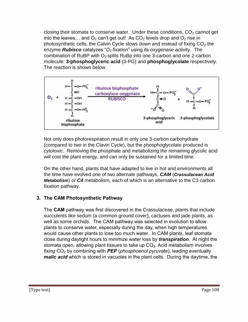
[Type text] Page 108

closing their stomata to conserve water. Under these conditions, CO2 cannot get

into the leaves… and O2 can’t get out! As CO2 levels drop and O2 rise in

photosynthetic cells, the Calvin Cycle slows down and instead of fixing CO2 the

enzyme Rubisco catalyzes “O2 fixation” using its oxygenase activity. The

combination of RuBP with O2 splits RuBp into one 3-carbon and one 2-carbon

molecule: 3-phosphoglyceric acid (3-PG) and phosphoglycolate respectively.

The reaction is shown below.

Not only does photorespiration result in only one 3-carbon carbohydrate

(compared to two in the Clavin Cycle), but the phosphoglycolate produced is

cytotoxic. Removing the phosphate and metabolizing the remaining glycolic acid

will cost the plant energy, and can only be sustained for a limited time.

On the other hand, plants that have adapted to live in hot arid environments all

the time have evolved one of two alternate pathways, CAM (Crassulacean Acid

Metabolism) or C4 metabolism, each of which is an alternative to the C3 carbon

fixation pathway.

3. The CAM Photosynthetic Pathway

The CAM pathway was first discovered in the Crassulaceae, plants that include

succulents like sedum (a common ground cover), cactuses and jade plants, as

well as some orchids. The CAM pathway was selected in evolution to allow

plants to conserve water, especially during the day, when high temperatures

would cause other plants to lose too much water. In CAM plants, leaf stomata

close during daylight hours to minimize water loss by transpiration. At night the

stomata open, allowing plant tissues to take up CO2. Acid metabolism involves

fixing CO2 by combining with PEP (phosphoenol pyruvate), leading eventually

malic acid which is stored in vacuoles in the plant cells. During the daytime, the

[Type text] Page 109

stored malic acid retrieved from the vacuoles enters chloroplasts, where it is split

into pyruvate and CO2. The latter then enters the Calvin Cycle to make glucose

and the starches. The CAM pathway is described below.

In sum, the CAM plants

open stomata to collect, fix and store CO2 as an organic acid at night.

close stomata to conserve water in the daytime.

re-fix the stored CO2 as carbohydrate using the NADPH and ATP from the

light reaction the next the day.

[Type text] Page 110

4. The C4 Photosynthetic Pathway

C4 refers to the 4-carbon end-product of CO2 fixation, which is in fact the same

as in CAM metabolism; malic acid! As in the CAM pathway, PEP carboxylase is

the catalyst of carbon fixation in C4 metabolism that converts phosphoenol

pyruvate (PEP) to oxaloacetate (OAA) that is then reduced to malic acid, as

shown below.

PEP carboxylase catalysis rapid, in part because malic acid does not accumulate

in the mesophyll cells, but instead is rapidly transferred to adjacent bundle

sheath cells. The result is that CO2 fixation is more efficient than in CAM plants.

This in turn allows C4 plants to keep stomata open for CO2 capture (unlike CAM

plants), but closed at least part of the day to conserve water. As the 4-carbon

malic acid is oxidized to pyruvate (3 carbons!) in the bundle sheath cells, CO2 is

released directly to Rubisco for rapid fixation by the Calvin Cycle. This system

allows more efficient water use and faster carbon fixation under high heat, dry

conditions than does C3 photosynthesis. Corn is perhaps the best known C4

plant!

[Type text] Page 111

V. Some Final Thoughts on the Evolution of Respiration and

Photosynthesis.

If we assume that the abundance of chemical energy on our cooling planet favored the

formation of cells that could capture free energy from these nutrients. These first cells

would have extracted nutrient free energy by non-oxidative, fermentation pathways. And

they would have been voracious feeders, quickly depleting their environmental nutrient

resources. But for the evolution of at least some autotrophic life forms, life would have

reached a dead end! Phototrophs that could capture free energy directly from light (i.e.,

the sun) would soon have become the most abundant autotrophs, if for no other reason

than sunlight is ubiquitous and always available (at least during the day). To conclude,

photosynthesis existed before respiration. Therefore one might ask whether and when

respiration co-opted photosynthetic electron transport reactions that captured the

electrons from H2O needed to reduce CO2, turning those reactions to the task of burning

sugars back to H2O and CO2.

Some iText & VOP Key Words and Terms

active transport of protons

energy efficiency of glucose metabolism

PEP carboxylase

ATP synthase energy flow in glycolysis pH gradient

bacterial flagellum energy flow in the Krebs Cycle

pheophytin

C4 photosynthesis F1 ATPase photosynthesis

Calvin Cycle FAD Photosystems

CAM photosynthesis FADH2 proton gate

carotene Light-dependent reactions proton gradient

chemiosmotic mechanism

Light-independent reactions

proton pump

Chlorophyll a Malic acid PSI electron acceptor

Chlorophyll b mitochondria PSII electron acceptor

Coenzyme Q (CoEQ) molecular motor redox reactions

complex I, II, III, IV NAD+ reduced electron carriers

[Type text] Page 112

Crassulaceae NADH RUBISCO

cristal membrane NADP+ RuBP

Cyclic photophosphorylation

NADPH Splitting water

cytochromes outer membrane stoichiometry of glycolysis

Dark Reactions oxidative phosphorylation stoichiometry of the Krebs Cycle

electrochemical gradient

oxidative phosphorylation substrate-level phosphorylation

electron transport system (chain)

P680 Z-scheme

endosymbiotic theory P700

[Type text] Page 113

Chapter 8: DNA Structure, Chromosomes,

Chromatin and Replication

The Double Helix; Chromosomes and Chromatin; Semi-Conservative

Replication; Replication Details

I. Introduction

In this chapter we look first at classic experiments that led to our understanding that

genes are composed of DNA. Then we look at the equally classic work of Watson,

Crick, Franklin and Wilkins that revealed the structure of the genetic molecule. Since

genes had been mapped to chromosomes since early in the 20th century, it was clear

that genes made up of DNA would be on chromosomes, so one section of this chapter

looks at this association. But chromosomes are a very discrete highly condensed

structures in eukaryotic cells that are visible only while the cells are dividing (i.e., during

mitosis or meiosis). At other times, during the much longer interphase portion of the cell

cycle, the DNA exists as part of a chromatin, a less organized form of chromosomal

material in the nucleus. In both chromosomes and chromatin, DNA is associated with

nuclear proteins. As we will see here and in a later chapter, understanding the

organization of DNA and proteins in chromatin is vital to our understanding of how and

when genes are expressed (turned on and off). Therefore, another section of the

chapter looks at DNA as part of chromatin. Then we’ll look at the molecular mechanism

of replication. We’ll see experiments done initially in bacteria, whose DNA is basically

just a circular DNA molecule that is not wrapped up in proteins or RNA. The

mechanisms to be described for this ‘naked’ prokaryotic and for replication of eukaryotic

DNA surrounded by proteins will differ precisely because of these differences in DNA

packing. Nevertheless, the molecular details of the process are quite similar overall,

speaking to an early and common evolutionary origin of replication.

Voice-Over PowerPoint presentations

The Stuff of Genes VOP

DNA Structure VOP

DNA & Chromosomes VOP

DNA & Chromatin VOP

Replication Part 1 VOP

Replication Part 2 VOP

[Type text] Page 114

Learning Objectives

When you have mastered the information in this chapter and the associated VOPs, you

should be able to:

1. discuss how Erwin Chargaff’’s data on the base ratios in DNA from different species

is consistent with DNA as the “stuff of genes”.

2. describe the experiments and interpret the results of Griffith, Avery et al. and

Hershey & Chase, each in the context of when the experiments were done.

3. state evidence that led to acceptance that genes are made of DNA and not proteins.

4. list and explain the evidence Watson and Crick used to build their model of DNA.

5. describe the organization of DNA in chromatin and chromosomes.

6. speculate on how this organization impacts replication.

7. list the key “actors” (proteins and enzymes) required for replication.

8. describe the actions and activities of proteins and enzymes required for replication.

9. define a viral infection.

10. trace the fate of 35SO4 (sulfate) into proteins synthesized in cultured bacteria.

11. compare and contrast the structure and functionality of different forms of chromatin.

12. outline an experiment to purify histone H1 from chromatin.

13. formulate an hypothesis for how histones evolved in eukaryotes and not in bacteria.

II. The Stuff of Genes By the late 19th century, the nucleus was known to be a major feature common to all

eukaryotic cells. By the dawn of the 20th century, the nucleus was thought likely to be

the seat of genetic information. At the same time, nuclei were shown histologically to be

made up mainly of proteins and DNA. DNA was believed to be a small, simple

molecule made up of 4 nucleotides (see DNA Structure below for a bit more historical

perspective). Following the re-discovery of Mendel’s Laws of Inheritance at about the

same time, the number of known inherited traits in any given organism increased

rapidly. As a result, early geneticists figured that DNA was too small and simple a

molecule to account for the inheritance of so many different physical traits. Early in the

20th century, enzyme activities were also inherited, just like morphological

characteristics. This led to the one-gene-one enzyme hypothesis. When enzymes

were shown to be proteins, the hypothesis became one-gene-one protein, and when

proteins were shown to be composed of one or more polypeptides, the final hypothesis

was one-gene-one-polypeptide. Because polypeptides were found to be long chains of

up to 20 different amino acids, polypeptides and proteins had the potential for enough

structural diversity to account for the growing number of heritable traits in a given

organism. Thus proteins seemed more likely candidates for the molecules of

inheritance. The experiments you will read about here occurred from the beginning of

[Type text] Page 115

World War I and lasted until just after World War 2. During this time we learned that

DNA was no mere tetramer, but was in fact a long polymer. We’ll see how some very

clever experiments eventually forced the scientific community to the conclusion that

DNA, not protein, was the genetic molecule, even with only 4 monomeric units.

A. Griffith’s Experiment

Fred Neufeld, a German bacteriologist studying pneumococcal bacteria in the early

1900s discovered 3 immunologically different strains of Streptococcus pneumonia

(Types I, II and III). The virulent strain (Type III) was responsible for much of the

mortality during the Spanish Flu (influenza) pandemic of 1918-1920. This

pandemic killed between 20 and 100 million people, mostly because the influenza

viral infection weakened the immune system of infected individuals, making them

susceptible to bacterial infection by streptococcus pneumonia. In the 1920s,

Frederick Griffith was working with the wild type virulent (Type III) and a benign

(Type II) strain of this bacterium to explore whether the Type II strain cells could

immunize mice against the virulent strain. The two strains were easy to tell apart

because the virulent strain grew in morphologically smooth colonies, while the

benign strain formed rough colonies. We now know that the smooth-colony forming

cells are coated with a polysaccharide capsule that makes colonies look smooth to

the naked eye, while the rough colony cells grow into colonies that do not shine, and

look rough because they lack the polysaccharide coating. The polysaccharide

capsule protects the virulent cells from the infected host organism’s immune system.

Lacking the polysaccharide coat, the R cells are attacked and cleared by the host

cell’s immune system before a serious infection can take hold. The experimental

design and results that Griffith published in 1928 are summarized in this illustration.

[Type text] Page 116

In the experiment, mice injected with benign (R, or rough) strain cells survived, and

no bacterial cells were found thereafter in the blood of these mice. Mice injected

with virulent (S, or smooth) strain cells died after a day, and their blood was full of S

cells. As expected, if a colony of S cells was heated to kill them before injecting

them into mice, the mice survived, and contained no bacterial cells in their blood.

This result was “expected” because heating had the same effect on the S cells as

pasteurization had on bacteria in milk!

In one experiment, Griffith injected a mixture of live R cells and heat-killed S cells,

presumably in the hope that the combination would induce immunity on the mouse.

You can imagine his surprise when the injected mice died after a day and that their

blood was filled with S cells. Griffith realized that something important had

happened in his experiments, namely that in the mix of live R cells and heat-killed S

cells, some R cells had become transformed by something from the dead S cells.

Bacterial transformation is in fact the acquisition of a genetic molecule (Griffith

called it the transforming principle) from the S cell debris by the live R cells. Thus,

the transformation made some of the R cells virulent. Griffith’s experiment opened

the way to experiments establishing that DNA, and not protein, is the “stuff of

genes”.

B. Avery-MacLeod-McCarty Experiment

A technique developed in the 1930’s demonstrated that R cells could be transformed

in vitro, that is, without the help of a mouse. With this technique, O. Avery, C.

MacLeod, and M. McCarty reported purifying heat-killed S-cell components (DNA,

proteins, carbohydrates, lipids…) and separately testing the transforming ability of

each molecular component on R cells. Their experiment is summarized below.

[Type text] Page 117

Since only the DNA fraction of the dead S cells could cause transformation, Avery

et al. concluded that DNA must be the Transforming Principle.

In spite of the results of Avery et al. many respected scientists still believed that

polypeptides (with their seemingly endless combinations of 20 amino acids) had the

biological specificity necessary to be genes. While they acknowledged to be a large

polymer, they still thought that DNA was that simple molecule, for example a

polymer mate up of repeating sequences of the 4 nucleotides with a simple base

sequence such as …AGCTAGCTAGCTAGCTAGCT…, a sequence without the

diversity needed to account for the many proteins that were known to be encoded by

genes. To adapt Marshal McLuhan’s famous statement that the medium is the

message (meaning that the airwaves don’t merely convey a message), many still

believed that proteins are the medium of genetic information as well as the functional

meaning of the message.

This position became increasingly untenable as the Avery et al. results were

confirmed following the inheritance of other genetic characteristics. But it was the

key experiment of Alfred Hershey and Martha Chase that put to rest any notion that

proteins were genes.

C. Hershey-Chase Experiment

Alfred Hershey and Martha Chase knew the life-cycle of bacterial viruses, called

bacteriophage (or phage for short), illustrated below.

Phages are inert particles until they infect bacterial cells. They start an infection

when they bind to the bacterial cell surface. Electron microscope studies revealed

the phage particle on the outside of the bacterium. Using a blender (not unlike a

kitchen blender), it was possible to “shake” off the phage particles from the bacterial

[Type text] Page 118

cells. Centrifugation could then bring the bacterial cells to a pellet at the bottom of

the centrifuge tube, leaving the detached ‘phage’ particles in the supernatant above

the pellet. If the pelleted cells had been attached to the phage for a short time they

would survive and reproduce when re-suspended in growth medium. But if the

mixture was incubated long enough (a few hours) before blending and

centrifugation, the re-suspended bacterial pellet would go on and lyse, producing

new phage. So, it took a few hours for the genetic information in the virus to be

transferred to the infected cell. This genetic material was apparently no longer

associated with the capsule of the phage particle, which could be recovered from the

centrifugal supernatant.

Hershey and Chase wanted to demonstrate that it was the DNA enclosed by the

viral protein capsule that actually caused the phage to infect the bacterium, and not

the capsule protein. In the experiment they designed, they separately grew E. coli

cells infected with T2 bacteriophage in the presence of either 32P or 35S, radioactive

isotopes of phosphorous and sulfur, respectively. The result was to produce phage

that contained either radioactive DNA or radioactive proteins, but not both (recall that

only DNA contains phosphorous and only proteins contain sulfur). They then

separately infected fresh E. coli cells with either 32P- or 35S-labeled, radioactive

phage. Their experiment is described below.

[Type text] Page 119

After allowing just enough time for infection after mixing phage with the bacterial

cells, some of the cells from each experiment were allowed to go on and lyse to

prove that they had become infected. The remainder of each mixture was sent to

the blender. After centrifugation of each blend, the pellets and supernatants were

examined to see where the radioactive proteins or DNA had gone. From the results,

the 32P always ended up in the pellet of bacterial cells while the 35S was found in the

phage remnant supernatant. Hershey and Chase concluded that the genetic

material of bacterial viruses was DNA and not protein, just as Avery et al. had

suggested that DNA was the bacterial transforming principle. But given the earlier

resistance to “simple” DNA being the genetic material they used cautious language

in framing their conclusions. They needn’t have; all subsequent experiments

confirmed that DNA was the genetic material. Concurrent with these confirmations

were experiments demonstrating that DNA might not be (indeed, was not) such a

simple, uncomplicated molecule!

III. DNA Structure

A. Early Clues and Ongoing Misconceptions

By 1878, a substance in the pus of battle-wounded soldiers derived from cell nuclei

(called nuclein) was shown to be composed of 5 bases (the familiar ones of DNA

and RNA). In the early 1900’s it was suggested that the bases (as part of

nucleotides) were connected through the phosphate groups in short repeating

chains of 4 nucleotides. Acknowledged to be a large polymer by the time of Avery et

al.’s studies, DNA was still considered to be a simple molecule with a simple

nucleotide repeat structure… too simple to account for genes. After the Hershey

and Chase experiments, there were only few who did not accept that DNA was the

genetic material. The only question was how such a “simple” molecule could

account for all the genes in even a simple organism like a bacterium. With the

advent of the X-Ray crystallography, it became possible to look at the structure of

large molecules, including DNA. If a substance can be crystallized, X-rays beamed

through the crystal will be bent (diffracted) at angles revealing the regular molecular

structure of the crystal. William Astbury demonstrated that high molecular weight

DNA had just such a regular structure, which he interpreted as a polymer of bases

(nucleotides) stacked in a linear structure, each nucleotide separated from the next

by 0.34 nm. Astbury is also remembered for describing his use of X-ray

crystallography as “molecular biology”, the term we use today to cover replication,

transcription, translation, gene regulation and all aspects of biomolecular structure.

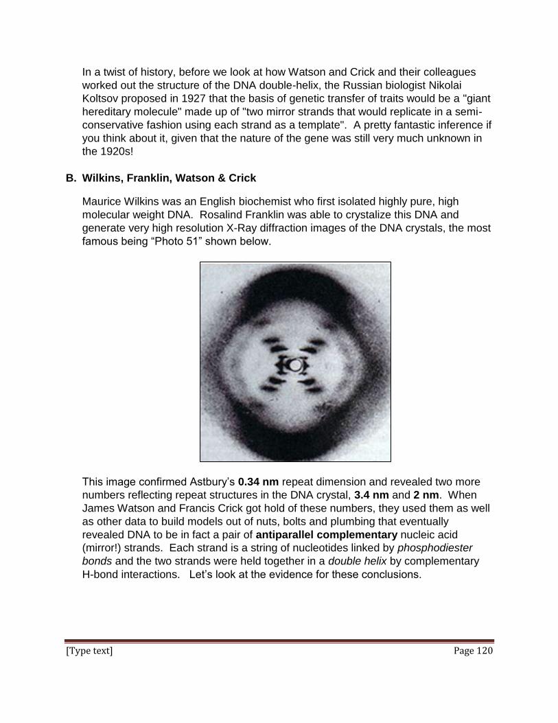
[Type text] Page 120

In a twist of history, before we look at how Watson and Crick and their colleagues

worked out the structure of the DNA double-helix, the Russian biologist Nikolai

Koltsov proposed in 1927 that the basis of genetic transfer of traits would be a "giant

hereditary molecule" made up of "two mirror strands that would replicate in a semi-

conservative fashion using each strand as a template". A pretty fantastic inference if

you think about it, given that the nature of the gene was still very much unknown in

the 1920s!

B. Wilkins, Franklin, Watson & Crick

Maurice Wilkins was an English biochemist who first isolated highly pure, high

molecular weight DNA. Rosalind Franklin was able to crystalize this DNA and

generate very high resolution X-Ray diffraction images of the DNA crystals, the most

famous being “Photo 51” shown below.

This image confirmed Astbury’s 0.34 nm repeat dimension and revealed two more

numbers reflecting repeat structures in the DNA crystal, 3.4 nm and 2 nm. When

James Watson and Francis Crick got hold of these numbers, they used them as well

as other data to build models out of nuts, bolts and plumbing that eventually

revealed DNA to be in fact a pair of antiparallel complementary nucleic acid

(mirror!) strands. Each strand is a string of nucleotides linked by phosphodiester

bonds and the two strands were held together in a double helix by complementary

H-bond interactions. Let’s look at the evidence for these conclusions.

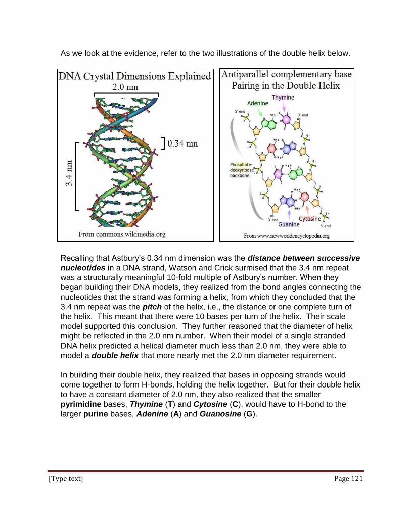
[Type text] Page 121

As we look at the evidence, refer to the two illustrations of the double helix below.

Recalling that Astbury’s 0.34 nm dimension was the distance between successive

nucleotides in a DNA strand, Watson and Crick surmised that the 3.4 nm repeat

was a structurally meaningful 10-fold multiple of Astbury’s number. When they

began building their DNA models, they realized from the bond angles connecting the

nucleotides that the strand was forming a helix, from which they concluded that the

3.4 nm repeat was the pitch of the helix, i.e., the distance or one complete turn of

the helix. This meant that there were 10 bases per turn of the helix. Their scale

model supported this conclusion. They further reasoned that the diameter of helix

might be reflected in the 2.0 nm number. When their model of a single stranded

DNA helix predicted a helical diameter much less than 2.0 nm, they were able to

model a double helix that more nearly met the 2.0 nm diameter requirement.

In building their double helix, they realized that bases in opposing strands would

come together to form H-bonds, holding the helix together. But for their double helix

to have a constant diameter of 2.0 nm, they also realized that the smaller

pyrimidine bases, Thymine (T) and Cytosine (C), would have to H-bond to the

larger purine bases, Adenine (A) and Guanosine (G).

[Type text] Page 122

Now to the question of how a “simple” DNA molecule could have the structural

diversity needed to encode thousands of different polypeptides and proteins…

Earlier studies in which E. coli DNA was purified, chemically hydrolyzed and shown

to contain nearly equal amounts of each base reinforced the notion that DNA was

that simple molecule that could not encode genes. But Watson and Crick had private

access to some revealing data from Erwin Chargaff’s base composition studies.

Chargaff found that the base composition of DNA from different species was not

always equimolar, that is the DNA was not composed of equal amounts of each of

the 4 bases. Some of this data is shown below.

The mere fact that DNA from some species could have different base compositions

that deviated from an equimolar base composition put to rest the argument that DNA

had to be a very simple sequence. Finally it was safe to accept that to accept the

obvious, namely that DNA was indeed the “stuff of genes”. Chargaff’s data also

showed a unique pattern of base ratios. Even though base compositions could vary

between species, the A/T and G/C ratio was always 1 for all species. Likewise the

ratio of (A+C)/(G+T) and (A+G)/(C+T) ratios. From this evidence, Watson and

Crick inferred that A would H-bond with T and G with C in the double helix. When

building their model with this new information, they also found H-bonding between

the complementary bases would be maximal only if the two DNA strands were

antiparallel, leading to the most stable structure of the double helix.

Watson and Crick published their conclusions about the structure of DNA in 1953

(click here to locate the article: Molecular Structure of Nucleic Acids: A Structure for

Deoxyribose Nucleic Acid). This article is famous for predicting a semiconservative

mechanism of replication, something as we’ve seen had been predicted by Koltsov

26 years earlier, albeit based on intuition… and much less evidence!

Watson, Crick and Wilkins received a Nobel Prize for their work on DNA structure in

1962. While there remains controversy surrounding the fact the Franklin did not

receive credit for this discovery, she had died in 1958, and at the time, Nobel prizes

were not awarded posthumously.

[Type text] Page 123

Final confirmation of Watson & crick’s suggestion of semiconservative replication

came from Meselson and Stahl’s very elegant experiment, which tested three

possible models of replication, shown below.

IV. Chromosomes

That chromosomes contained genes was understood from the start of the 20th century.

Therefore it becomes necessary to understand the relationship between chromosomes,

chromatin, DNA and genes. As noted earlier, chromosomes are really a specialized,

condensed version of chromatin. The main structural features of a chromosome are

shown below.

We now know that the compact structure of chromosomes prevents damage to the DNA

that might otherwise occur as chromatids are pulled apart by forces on centromeres

generated by mitotic or meiotic spindle fibers. Late 19th century observations of

[Type text] Page 124

chromosome behavior during cell division pointed to a role in heredity. Chromosomes

were seen to condense from the dispersed cytoplasmic background remaining after the

nucleus itself breaks down during both mitosis and meiosis. Thus early on,

chromosomes were quickly seen as playing a role in heredity. A recent computer-

colorized cell in mitosis is shown below.

When cells in mitosis are placed under pressure, the cells burst and the chromosomes

spread apart. Such a chromosome spread is shown below.

The number, sizes and shapes of chromosomes were shown to be species-specific.

Finally, a close look at spreads from different species revealed that chromosomes came

in morphologically matched pairs. This was so reminiscent of Gregor Mendel’s paired

Human Chromosomes

Mitotic chromosomes spread by

bursting cells in mitosis, stained

to reveal morphological

variation along their lengths.

From:

http://essayweb.net/biology/chromatid.shtml

[Type text] Page 125

hereditary factors that chromosomes were widely accepted as the structural seat of

genetic inheritance. The morphological pairing of chromosomes can readily be seen in

a karyotype, created by cutting apart a micrograph like the one above with a pair of

scissors and matching the chromosomes. The paired homologous chromosomes in the

human female karyotype shown below are easily identified.

Captured in mitosis, all dividing human cells contain 46 chromosomes that can be

karyotyped. In this karyotype, the duplicated chromatids have not yet separated,

indicating that the chromosomes were spread from metaphase cells. These

chromosomes are from a female cell; note the homologous sex (“X”) chromosome pair

at the upper right of the karyotype. The X and Y chromosomes of males are aligned

when creating a karyotype, but these chromosomes are not truly homologous.

Chromosomes in both the original spread and in the aligned karyotype have been

stained, revealing morphological markings that help distinguish the chromosomes and

their homologs.

From: http://labspace.open.ac.uk/mod/resource/view.php?id=419219

[Type text] Page 126

V. Genes and Chromatin

Chromosomes and chromatin are a uniquely eukaryotic association of DNA with more

or less protein. Bacterial DNA (and prokaryotic DNA generally) is relatively ‘naked’ – not

visibly associated with protein.

If chromosomes represent the most condensed form of chromatin, then the electron

micrograph of a eukaryotic cell below reveals that interphase cell chromatin can itself

exist in various state of condensation.

During interphase chromatin can undergo a transition between the more condensed

heterochromatin and the less condensed euchromatin. These transitions involve

changes in the amounts and types of proteins bound to the chromatin that can occur as

genes are regulated (activated or silenced). Active genes tend to be in the more

dispersed in euchromatin so that enzymes of replication and transcription have easier

access to the DNA. Genes that are inactive in transcription are heterochromatic,

obscured by chromatin proteins present in heterochromatin. We’ll be looking at some

experiments that demonstrate this in a later chapter.

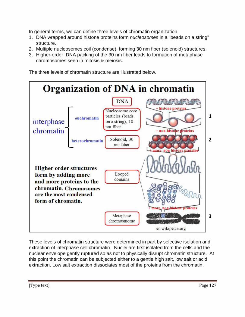
[Type text] Page 127

In general terms, we can define three levels of chromatin organization:

1. DNA wrapped around histone proteins form nucleosomes in a "beads on a string"

structure.

2. Multiple nucleosomes coil (condense), forming 30 nm fiber (solenoid) structures.

3. Higher-order DNA packing of the 30 nm fiber leads to formation of metaphase

chromosomes seen in mitosis & meiosis.

The three levels of chromatin structure are illustrated below.

These levels of chromatin structure were determined in part by selective isolation and

extraction of interphase cell chromatin. Nuclei are first isolated from the cells and the

nuclear envelope gently ruptured so as not to physically disrupt chromatin structure. At

this point the chromatin can be subjected either to a gentle high salt, low salt or acid

extraction. Low salt extraction dissociates most of the proteins from the chromatin.

1

2

3

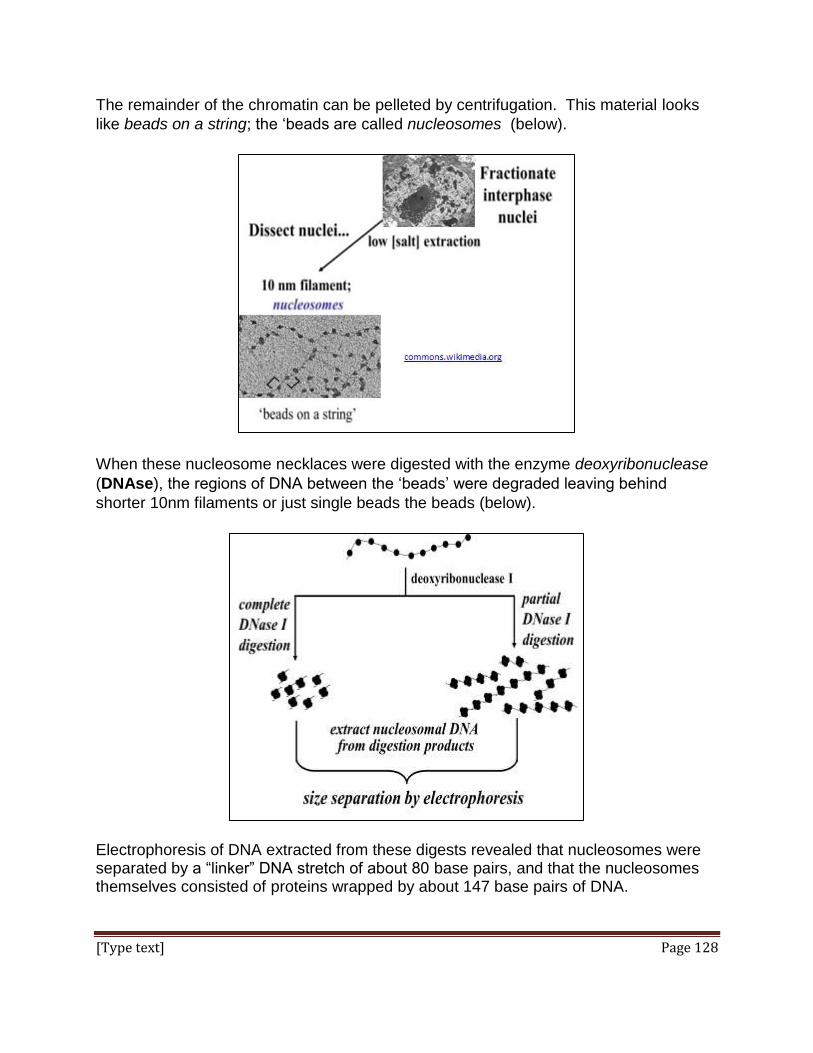
[Type text] Page 128

The remainder of the chromatin can be pelleted by centrifugation. This material looks

like beads on a string; the ‘beads are called nucleosomes (below).

When these nucleosome necklaces were digested with the enzyme deoxyribonuclease

(DNAse), the regions of DNA between the ‘beads’ were degraded leaving behind

shorter 10nm filaments or just single beads the beads (below).

Electrophoresis of DNA extracted from these digests revealed that nucleosomes were separated by a “linker” DNA stretch of about 80 base pairs, and that the nucleosomes themselves consisted of proteins wrapped by about 147 base pairs of DNA.

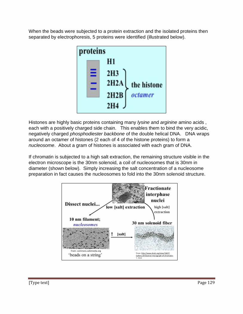
[Type text] Page 129

When the beads were subjected to a protein extraction and the isolated proteins then

separated by electrophoresis, 5 proteins were identified (illustrated below).

Histones are highly basic proteins containing many lysine and arginine amino acids ,

each with a positively charged side chain. This enables them to bind the very acidic,

negatively charged phosphodiester backbone of the double helical DNA. DNA wraps

around an octamer of histones (2 each of 4 of the histone proteins) to form a

nucleosome. About a gram of histones is associated with each gram of DNA.

If chromatin is subjected to a high salt extraction, the remaining structure visible in the

electron microscope is the 30nm solenoid, a coil of nucleosomes that is 30nm in

diameter (shown below). Simply increasing the salt concentration of a nucleosome

preparation in fact causes the nucleosomes to fold into the 30nm solenoid structure.

high [salt] extraction

From: http://www.dnalc.org/view/16637-Gallery-29-Electron-micrograph-of-chromatin-1-.html

From: commons.wikimedia.org

[Type text] Page 130

As you might guess, an acidic extraction should selectively remove the basic histone

proteins, leaving behind an association of DNA with non-histone proteins. This proved

to be the case, and an electron micrograph of the chromatin remnant after an acid

extraction of metaphase chromosomes is shown below.

The DNA, freed of the regularly spaced histone based nucleosomes, loops out away

from the long axis of the chromatin. The dark material, labeled scaffold protein, makes

up most of what is left after removal of the histones, and much of this protein is the

enzyme topoisomerase. As we will see, topoisomerases prevent DNA from breaking

apart under the strain of replication.

And this brings us to replication itself.

[Type text] Page 131

VI. DNA Replication

DNA strands have directionality, with a 5’ nucleotide-phosphate and a 3’ deoxyribose

hydroxyl end. Because the strands of the double helix are antiparallel, the 5’ end of

one strand aligns with the 3’end of the other at both ends of the double helix. The

complementary pairing of bases in DNA means that the information contained on a

single strand could be used as a template to make a new complementary strand. As

we’ll see, this structure of DNA created some interesting dilemmas for understanding

the biochemistry of replication. The puzzlement surrounding how replication proceeds

begins with experiments that visualize replicating DNA.

A. Visualizing Replication and Replication Forks

Geneticists had already determined that bacterial chromosomes were circular before

John Cairns confirmed this fact by direct visualization. He grew E. coli cells for long

periods on 3H-thymidine (3H-T) to make all of their DNA radioactive. He then

treated the cells to gently break them open and release their DNA. The DNA was

allowed to settle on membranes to which the DNA adhered. A radiation sensitive

film was layered onto the membrane to allow the radiation to expose the film,

creating an autoradiograph that which was then examined in the electron

microscope.

Cairns saw tracks of silver grains in the exposed film of his autoradiographs (the

same kind of silver grains that create an image on film in old-fashioned

photography). A sampling of his autoradiographic images is illustrated below.

[Type text] Page 132

Cairns measured the length of the “silver” tracks, which usually consisted of three

possible closed loops, or circles. Two of these circles were always equal in length,

with a circumference that was virtually predicted by the DNA content of a single,

non-dividing cell. Cairns therefore interpreted these images to be bacterial DNA in

the process of replicating, and arranged a sequence of images of disparate

autoradiographs to make his point (illustrated below).

Because the replicating chromosomes looked (rather vaguely!) like the Greek letter

, he called them theta images. Cairns inferred that replication started at a single

point on the bacterial chromosome, the origin of replication. Subsequent

experiments demonstrated that replication did indeed begin at an origin of

replication, after which the double helix was unwound and replicated away from the

origin in both directions, forming two replication forks, (illustrated below).

[Type text] Page 133

Bacterial cells can divide every hour or even less, meaning that the rate of bacterial

DNA synthesis is about 2 X 106 base pairs per hour. A nucleus of a typical

eukaryotic cell contains thousands of times as much DNA in their nucleus compared

to bacteria, and even a small chromosome can contain hundreds or thousands of

times as much DNA as a bacterium. Thus eukaryotic cells cannot afford to double

their DNA at a bacterial rate of replication! This problem was solved not by evolving

a faster biochemistry of replication, but by evolving multiple origins of replication

from which DNA synthesis proceeds in both directions, creating replicons that

eventually meet to complete replication of linear chromosomes.

Before we consider the biochemical events of replication at replication forks in detail,

let’s look at the role of DNA polymerase enzymes in the process.

B. DNA Polymerases Catalyze Replication

All DNA polymerases require a template strand against which to synthesize a new

complementary strand. And all grow new DNA by adding to the 3’ end of the

growing DNA chain in successive condensation reactions. All DNA polymerases

also have the odd property that they can only add to a pre-existing strand of nucleic

acid, raising the question of where the ‘pre-existing’ strand comes from! The

reaction catalyzed by DNA polymerases forms a phosphodiester linkage between

the end of a growing strand and the incoming nucleotide complementary to the

template strand. The energy for the formation of the phosphodiester linkage comes

in part from the hydrolysis of two phosphates (pyrophosphate) from the incoming

nucleotide during the reaction.

[Type text] Page 134

Replication requires the participation of many nuclear proteins in both prokaryotes

and eukaryotes. But all of the basic steps of replication are performed by the DNA

polymerase enzyme itself, as shown in the illustration below.

DNA polymerases replicate DNA with high fidelity, with as few as one error per 107

nucleotides. But mistakes do occur. Thanks to the proofreading ability of some

DNA polymerases, mistakes are most often corrected. The polymerase can sense a

mismatched base pair, slow down and then catalyze repeated hydrolyses of

nucleotides until it reaches the mismatched base pair (shown below).

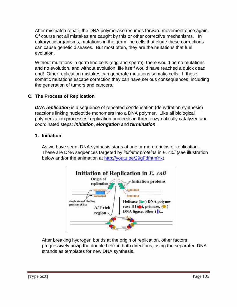
[Type text] Page 135

After mismatch repair, the DNA polymerase resumes forward movement once again.

Of course not all mistakes are caught by this or other corrective mechanisms. In

eukaryotic organisms, mutations in the germ line cells that elude these corrections

can cause genetic diseases. But most often, they are the mutations that fuel

evolution.

Without mutations in germ line cells (egg and sperm), there would be no mutations

and no evolution, and without evolution, life itself would have reached a quick dead

end! Other replication mistakes can generate mutations somatic cells. If these

somatic mutations escape correction they can have serious consequences, including

the generation of tumors and cancers.

C. The Process of Replication

DNA replication is a sequence of repeated condensation (dehydration synthesis)

reactions linking nucleotide monomers into a DNA polymer. Like all biological

polymerization processes, replication proceeds in three enzymatically catalyzed and

coordinated steps: initiation, elongation and termination.

1. Initiation

As we have seen, DNA synthesis starts at one or more origins or replication.

These are DNA sequences targeted by initiator proteins in E. coli (see illustration

below and/or the animation at http://youtu.be/29gFdfhtmYk).

After breaking hydrogen bonds at the origin of replication, other factors

progressively unzip the double helix in both directions, using the separated DNA

strands as templates for new DNA synthesis.

[Type text] Page 136

Sequences that bind to initiation proteins tend to be rich in adenine and thymine

bases. This is because A-T base pairs have two hydrogen bonds that require

less energy to break than the three hydrogen bonds holding G-C pairs together.

Once the hydrogen bonds at the origin of replication have been loosened, DNA

helicase, DNA primase, DNA polymerase III and other proteins are recruited to

the site. Helicase uses energy from ATP to unwind the double helix and DNA

polymerase III is the main enzyme that elongates new DNA. At this point, two

replication forks have formed on either side of a replication bubble (nascent

replicon), and replication can begin with repeated cycles of elongation.

All DNA replication requires the free 3' hydroxyl group of a pre-existing nucleic

acid strand to which the DNA polymerase will add additional nucleotides. This

strand is called the primer, and the question is, where does the primer come

from? Since RNA polymerases (enzymes that catalyze RNA synthesis) can

synthesize a new nucleic acid strand from scratch (i.e., from the first base), it was

suggested that a short RNA primer would be made to which new

deoxynucleotides would be added by DNA polymerase. In fact, cells use the

primase (a specialized RNA polymerase) to synthesize the short RNA primer

required for elongation by DNA polymerase.

2. Elongation

If we look at elongation at one replication fork (below), we can see a problem:

One of the two new DNA strands can grow continuously towards the replication

fork as the double helix unwinds. But what about the other strand? Either the

other strand must either grow in pieces in the opposite direction, or must wait to

begin synthesis until the double helix is fully unwound.

[Type text] Page 137

When mutants of T4 phage that grew slowly in their E. coli host cells were isolated, Okazaki and Okazaki showed that the cause was a mutation in the gene for the enzyme called DNA ligase. This enzyme was required to “stitch together” the ends of linear phage DNA to generate its circular “chromosome”. The data on T4 phage growth of wild type and mutant T4 phage is summarized below.

This suggested the hypothesis that DNA ligase plays a role in the discontinuous

synthesis of DNA. The hypothesis was that DNA replicated against the lagging

strand template was synthesized in fragments that were then linked in a

dehydration synthesis reaction by DNA ligase to form phosphodiester linkages

between DNA fragments, as illustrated below.

[Type text] Page 138

When the hypothesis was tested, the Okazakis found that short DNA fragments

did indeed accumulate in E. coli cells infected with ligase-deficient mutants, but

not in cells infected with wild type phage. The lagging strand fragments are

called Okazaki fragments after their discoverers.

But this scenario creates another dilemma! Each Okazaki fragment would have

to begin with a 5’ RNA primer. This primer would have to be removed and

replaced with DNA nucleotides before the fragments were stitched together by

DNA ligase. This in fact happens, and the process illustrated below.

Removal of the RNA primer nucleotides requires the action of DNA polymerase I.

This enzyme has a 5’-exonuclease activity that can catalyze hydrolysis of

phosphodiester bonds between the RNA (or DNA) nucleotides from the 5’-end of

a nucleic acid strand. At the same time that the RNA nucleotides are removed,

DNA polymerase I catalyzes their replacement by the appropriate deoxy-

nucleotides. Finally, when each fragment is entirely DNA, DNA ligase links it to

the rest of the discontinuously-growing DNA strand.

[Type text] Page 139

Because of its 5’ exonuclease activity (not found in other DNA polymerases),

DNA polymerase 1 also plays unique roles in DNA repair.

As Cairn’s suggested and others demonstrated, replication proceeds in two

directions from the origin to form the replication bubble, or replicon with its two

replication forks (RFs). Each RF has a primase associated with replication of

Okazaki fragments along lagging strand templates, as shown below.

We’ll look at how all of these replication activities might be coordinated after

considering what happens when replicons reach the ends of the linear

chromosomes of eukaryotes.

3. Termination

In prokaryotes, replication is complete when the two replication forks meet after

replicating their portion of the circular DNA molecule. In eukaryotes, the many

replicons fuse to become larger replicons, eventually reaching the ends of the

chromosomes. At that point, replication of linear DNA undergo a termination

process involving extending the length of one of the two strands by the enzyme

telomerase and replicating the extended DNA using DNA polymerase. This

complex set of reactions evolved in eukaryotes because without it, chromosomal

DNA would be shortened after each round of replication.

RF

RF

DNA

Primase

[Type text] Page 140

One of the more interesting recent observations was that differentiated, non-

dividing cells no longer produce the telomerase enzyme. On the other hand, the

telomerase gene is active in normal dividing cells (e.g., stem cells) and cancer

cells, which contain abundant telomerase.

The action of telomerase is summarized in the illustration below, and animated at

http://youtu.be/xdm4UpixaLU.

4. Replication is Processive

The drawing of the replicon above suggests separate events on each DNA

strand, but we now know that replication is processive, meaning that both new

DNA strands are made in the same direction at the same time. How is this

possible?

[Type text] Page 141

The illustration below shows that the lagging strand template DNA bends around

so that it faces in the same direction as the leading strand at the replication fork,

as shown in the illustration below.

The structure cartooned at the replication fork is called a replisome, and

consists of clamp proteins, primase, helicase, DNA polymerase, among other

proteins. Processive replication is animated at http://youtu.be/ThMSjtggNDo.

5. One last problem with replication

Cairns recorded many images of E. coli below.

[Type text] Page 142

The coiled, or twisted appearance of the replicating circles were interpreted to be

a natural consequence of trying to pull apart helically intertwined strands of

DNA… or in fact, intertwined strands of any material! As the strands continued to

unwind, it was reasoned that the DNA would twist into a kind of supercoiled DNA,

and that increased DNA unwinding would cause the phosphodiester bonds in the

DNA to rupture, fragmenting the DNA. Since this does not happen, experiments

to demonstrate the supercoiling phenomenon were devised, and hypotheses for

mechanism to relax the supercoils were suggested. Testing these hypotheses

revealed enzymes called topoisomerases which catalyze hydrolysis of

phosphodiester bonds, controlled unwinding of the double helix, and re-formation

of the phosphodiester linkages. It is important to note that the topoisomerases

are not part of a replisome, but can act far from a replication fork, probably

responding to the tensions in overwound DNA. Recall that the topoisomerases

comprise much of the protein lying along eukaryotic chromatin.

We have considered most of the molecular players in replication. Below is a list

of the key replication proteins and their functions (from DNA Replication in

Wikipedia:

[Type text] Page 143

Some iText & VOP Key Words and Terms

10 nm fiber helicase protein coat

30 nm fiber heterochromatin pyrophosphate

5' -to-3' replication high-speed blender replication

antiparallel DNA

strands histone octamer replication fork

bacteriophage histone proteins replication forks

base ratios influenza replicons

beads-on-a-string initiation replisome

bidirectional replication initiator proteins S phase of the cell cycle

Central Dogma karyotype

semi-conservative

replication

centromere lagging strand

single-strand binding

proteins

chromatin leading strand solenoid fiber

chromosomes lysis spindle fibers

clamp proteins metaphase chromatin S. pneumonia type III-S

condensation reactions mitosis & meiosis S. pneumonia type II-R

conservative

replication mutations supercoiling

deoxyribonuclease non-histone proteins T2 phage

discontinuous

replication nuclear proteins telomerase

dispersive replication nucleosomes telomeres

DNA Okazaki fragments tetranucleotide hypothesis

DNA ligase

levels of chromatin

packing theta images

DNA polymerase I, II

and III origin of replication topoisomerases

DNA repair phosphate backbone transforming principle

DNA topology phosphodiester linkage triplets genetic code

double helix primase viral infection

elongation primer X & Y chromosomes

euchromatin processive replication X-ray crystallography

genes proofreading X-ray diffraction

[Type text] Page 144

Chapter 9: Transcription and RNA Processing RNA Transcription, RNA Polymerases, Initiation, Elongation, Termination, Processing

I. Introduction

Transcription, the synthesis of RNA based on a DNA template, is the central step of the

Central Dogma proposed by Crick in 1958. The basic steps of transcription are the

same as for replication: initiation, elongation and termination. The differences are in the

details. For example, E. coli uses a single RNA polymerase enzyme to transcribe all

kinds of RNAs while eukaryotic cells use different RNA polymerases for ribosomal RNA

(rRNA), transfer RNA (tRNA) and messenger RNA (mRNA) synthesis. Recalling that

bacterial DNA is almost ‘naked’ while eukaryotic DNA is in a nucleus all wrapped up in

chromatin proteins, you might guess that RNA polymerases and other transcription

proteins need help accessing DNA in higher organisms. Another difference is that most

RNA transcripts in prokaryotes emerge from transcription ready to use. Eukaryotic

transcripts are typically synthesized as longer precursors that must be processed by

trimming or splicing (or both!). Another difference: in bacterial cells translation of an

mRNA can begin even before the transcript is finished. That’s because these cells have

no nucleus. In our cells, RNAs must exit he nucleus before they are used to make

proteins on ribosomes in the cytoplasm. In this chapter, you will encounter the three

major classes of RNA and detailed mechanisms of their transcription and (in

eukaryotes) their processing. You will also meet bacterial polycistronic mRNAs (mRNA

transcripts of operons that encode more than one polypeptide). We’ll introduce the

structural basis of DNA-protein interactions, looking at the structural motifs and domains

of nuclear proteins that are suited/fitted to recognizing and binding to sequences in

double-stranded DNA.

Voice-Over PowerPoint Presentations

Overview of Transcription

Transcription & Processing-Part 1 VOP

Transcription & RNA Processing-Part 2 VOP

Learning Objectives

When you have mastered the information in this chapter and the associated VOPs, you

should be able to:

1. discriminate between the 3 steps of transcription in pro- and eukaryotes, and the

factors involved in each.

2. state an hypothesis for why eukaryotes evolved complex RNA processing steps.

[Type text] Page 145

3. speculate on why any cell in its right mind would have genes containing introns and

exons so that their transcripts would have to be processed by splicing.

4. articulate the differences between RNA vs. DNA structure.

5. explain the need for sigma factors in bacteria.

6. speculate on why eukaryotes do not have operons.

7. list structural features of proteins that bind and recognize specific DNA sequences.

8. explain how proteins that do not bind specific DNA sequences can still bind to

specific regions of the genome.

9. formulate an hypothesis for why bacteria do not polyadenylate their mRNAs as much

as eukaryotes do.

10. formulate an hypothesis for why bacteria do not cap their mRNAs.

II. Overview of Transcription

A. The Major Types of Cellular RNA

All cells make three main kinds of RNA. Ribosomal RNA (rRNA) is a structural as

well as enzymatic component of ribosomes, the protein synthesizing machine in the

cytoplasm (illustrated below). Quantitatively, rRNAs are by far the most abundant

RNAs in the cell.

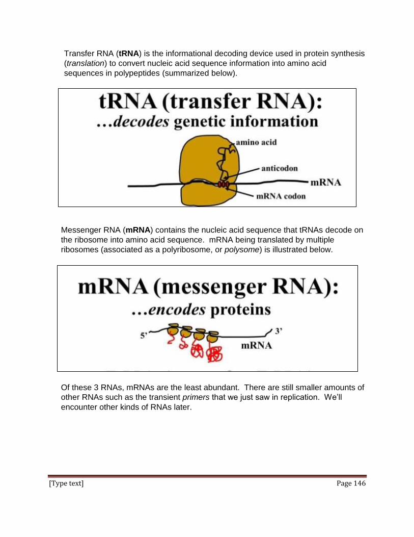
[Type text] Page 146

Transfer RNA (tRNA) is the informational decoding device used in protein synthesis

(translation) to convert nucleic acid sequence information into amino acid

sequences in polypeptides (summarized below).

Messenger RNA (mRNA) contains the nucleic acid sequence that tRNAs decode on

the ribosome into amino acid sequence. mRNA being translated by multiple

ribosomes (associated as a polyribosome, or polysome) is illustrated below.

Of these 3 RNAs, mRNAs are the least abundant. There are still smaller amounts of

other RNAs such as the transient primers that we just saw in replication. We’ll

encounter other kinds of RNAs later.

[Type text] Page 147

B. Key Steps of Transcription

In transcription, an RNA polymerase catalyzes synthesis of a complementary,

antiparallel RNA strand. RNA polymerases use ribose nucleotide triphosphate

(NTP) precursors, in contrast to DNA polymerases of replication which use

deoxyribose nucleotide (dNTP) precursors. In addition, RNAs incorporate uracil (U)

nucleotides into RNA strands instead of the thymine (T) nucleotides that end up in

new DNA. Also in contrast to replication, RNA polymerases do not require a primer.

With the help of transcription initiation factors, RNA polymerases recognize

transcription start sites in genes and can start a new nucleic acid strand from

scratch. Also, proofreading is less important during RNA synthesis. While this

means that there is a potential to make more mistakes during transcription than

during replication, transcription errors are less consequential than those made

during replication. The basic steps of transcription are summarized below:

Here we can identify several of the DNA sequences that characterize a gene. The

promoter is the binding site for RNA polymerase. It usually lies 5’ to, or upstream of

the transcription start site (the bent arrow). Binding of the RNA polymerase

positions the enzyme to start unwinding the double helix near the transcription start

site and to being synthesizing new RNA from that site. The grey regions in the 3

panels are the regions of DNA that will be transcribed. Termination sites are

typically 3’ to, or downstream from the transcribed region of the gene.

[Type text] Page 148

In bacteria, some transcription units encode more than one kind of RNA. Bacterial

operons are an example of this phenomenon, in which a single mRNA molecule

contains mRNA regions that are translated into more than one polypeptide (shown

below).

C. RNAs are Extensively Processed After Transcription in Eukaryotes

Transcription is the basic mechanism of gene expression. The DNA region that is

actually transcribed is a transcription unit. Transcription units include genes for

messenger RNA (mRNA) encoding polypeptides, ribosomal RNA (rRNA), transfer

RNA (tRNA) and a growing number of very short RNAs that help control the use of

the other kinds of RNAs. As we’ll see, many RNAs are transcribed into large pre-

RNAs that are processed (trimmed and/or chemically modified) to generate a mature

biologically active transcript.

[Type text] Page 149

Every pre-RNA (precursor RNA or primary transcript) contains in its sequence the

information necessary for its function in the cell. Processing of the three major

types of transcripts in eukaryotes is shown below.

1. Primary mRNA transcripts are spliced to remove internal sequences called

introns and to ligate the remaining coding regions of the message (called

exons) into a continuous mRNA. In some cases, the same pre-mRNA can be

transcribed into alternate mRNAs encoding related but not identical polypeptides!

2. Pre-ribosomal RNAs are cleaved and/or trimmed (not spliced!) to generate

shorter functional rRNAs.

3. Pre-tRNAs are trimmed, some bases within the transcript are modified and 3

bases (not encoded by the tRNA gene) are enzymatically added to the 3’-end

We’ll be looking at eukaryotic transcript processing in more detail later.

[Type text] Page 150

D. Transcription is Regulated: Genes Can be Turned On and Off

As we will see, transcription (gene expression) is controlled by the binding of

regulatory proteins to DNA sequences associated with the gene. Most of these

DNA regulatory sequences are relatively short and found upstream of the promoter

in the 5’-nontranscribed DNA. In eukaryotes, transcriptional regulatory sequences

are also found in the 3’-nontranscribed region of the gene, and even in introns (see

below). Often these regulatory DNA elements are quite far from the transcription

unit of the gene. In another chapter we’ll examine how regulatory proteins act to

control transcription both near, and at a sometimes considerable distance from a

gene.

Consider briefly that all DNA binding proteins must get past chromatin protein

guardians of the double helix. And even when they penetrate the chromatin protein

covering, they encounter a highly electronegative phosphodiester backbone. So

what is it that these proteins actually bind to? They “see” the base sequences in the

interior of the double helix, mainly through the major groove and to a lesser extent,

the minor groove. You can see how a bacterial regulatory protein with a helix-turn-

helix motif binds to two consecutive turns of the major groove (below).

As always in macromolecular interactions, shape plays a major role! Regions of

specific helices in the lambda repressor protein shown here are seen penetrating the

major groove.

[Type text] Page 151

III. Details of Transcription

A well written summary of transcription in prokaryotes and eukaryotes can be found in

an NIH website at Transcription in Prokaryotes and Eukaryotes. Here and at this link

you will encounter proteins that bind DNA. Some do so just to allow transcription, like

RNA polymerase and other proteins that must bind to the gene promoter to initiate

transcription). Others, the regulatory factors (like the lambda repressor proteins we just

saw) bind DNA to regulate transcription, inducing or silencing transcription of a gene.

The details of transcription and processing differ substantially in prokaryotes and

eukaryotes.

A. Prokaryotes

In E. coli, a single RNA polymerase transcribes all kinds of RNA. The RNA

polymerase associates with a sigma factor ( factor). This is a protein that binds to

the RNA polymerase to enable the enzyme to bind to the promoter sequence of a

gene. The first promoter sequence to be defined was called the Pribnow box after

its discoverer (illustrated below).

As shown, the bacterial genes can have one of several promoters, increasing

options for when a gene is active. Thus, bacteria can regulate which genes are

[Type text] Page 152

transcribed at a given moment by selectively controlling relative cellular

concentrations of the different factors. We shall see different modes of prokaryotic

gene regulation in the next chapter. Soon after transcription is initiated, the

factors fall off the RNA polymerase which continues to unwind the double helix

and to elongate the transcript. Elongation is the successive addition of nucleotides

complementary to their DNA templates, forming phosphodiester linkages. The

enzymatic reaction is similar to the DNA polymerase-catalyzed elongation of DNA

during replication.

There are two ways that bacterial RNA Polymerase ‘knows’ when it has reached the

end of a transcription unit, neither of which relies on a protein binding to a defined

sequence in DNA at the end of a gene! In one way, when the RNA polymerase

nears the 3’ end of the nascent transcript, it transcribes a 72 base, C-rich region. At

this point, a termination factor called the rho protein binds to the nascent RNA

strand. rho an ATP-dependent helicase that breaks H-bonds between the RNA and

the template DNA strand, thus preventing further transcription. rho-dependent

termination is illustrated below.

[Type text] Page 153

In the other mechanism of termination the polymerase transcribes RNA whose

termination signal assumes a secondary structure that then causes the dissociation

of the RNA Polymerase, template DNA and the new RNA transcript. This rho-

independent termination is illustrated below.

B. Eukaryotes

Whereas bacteria rely on a single RNA polymerase for their transcription needs,

eukaryotes use 3 different enzymes to synthesize the different kinds of RNA, as

shown below:

[Type text] Page 154

Transcription of eukaryotic mRNAs by RNA polymerase II requires the sequential

assembly of a eukaryotic Initiation Complex on the gene. This involves the

interaction of many proteins with a promoter, summarized below.

The typical eukaryotic promoter for a protein-encoding gene contains a TATA box

DNA sequence motif as well as additional short upstream sequences. TATA-

binding protein (TBP) first binds to the TATA box along with TFIID (transcription

initiation factor IID). This intermediate recruits TFIIA and TFIIB. Finally, TFGIIE,

TFIIF and TFIIH, several other initiation factors and finally RNA polymerase II bind to

form a transcription initiation complex. The 5’-terminus of the RNA polymerase is

then phosphorylated several times. After dissociation of some of the TF’s the

remaining RNA polymerase-TF complex starts elongation of the new RNA transcript.

[Type text] Page 155

Unlike prokaryotic RNA polymerase, eukaryotic RNA Polymerase II does not have

an inherent helicase activity. For this, eukaryotic gene transcription relies on the

multi-subunit TFIIH protein, in which two subunits have helicase activity. Consistent

with the closer relationship of archaea and eukaryotes (rather than prokaryotes),

transcription initiation in archaea and eukaryotes is similar, if somewhat less

involved. The complex is assembled at a TATA-box, but its formation in archaea

involves only RNA polymerase II, a TBP, and a TFIIB homologue called TFB.

Transcription of 5S rRNA and tRNAs by RNA Polymerase III is unusual in that the

promoter sequence to which it binds (with the help of initiation factors) is not

upstream of the transcribed sequence, but lies within the transcribed sequence

(below top). After binding to this internal promoter, the polymerase re-positions itself

to transcribe the RNA from the transcription start site (below middle). So, the final

transcript contains the promoter sequence (below bottom). The 5S rRNA and all

tRNAs are transcribed in this way by RNA polymerase III.

[Type text] Page 156

RNA Polymerase I and transcription initiation factors bind to rRNA gene promoters

upstream of the transcribed region to begin their transcription, though less is known

about the details of the process.

Likewise, transcription termination is not as well understood in eukaryotes as in

prokaryotes. In the case of mRNA synthesis, termination is coupled to the

polyadenylation processing step common to most mRNAs (discussed in more detail

below). A useful summary of what is known is presented at this link from the NIH-

NCBI website: Eukaryotic RNA Polymerase Termination Mechanisms.

IV. Details of Eukaryotic RNA Processing

A. The Two Sources of Ribosomal RNAs

1. One source is a large gene that encodes a precursor transcript containing three

size classes of rRNAs. From shortest to longest they are the 5.8S rRNA,

18SrRNA and 28S rRNA. The ‘S’ stands for Svedborg, the biochemist who

developed the sedimentation velocity ultra-centrifugation technique that

separates molecules like RNA by size. The higher the S value, the larger the

molecule and therefore the faster it moves through the viscous sugar gradient

during centrifugation. As shown in the illustration below, these rRNAs are

transcribed by RNA Polymerase I from large transcription units.

[Type text] Page 157

A 45S pre-rRNA transcript is then processed by cleavage. Actually, there are

many copies of the 45S rRNA gene in eukaryotic cells, as might be expected

since making proteins (and therefore ribosomes) will be an all-consuming cellular

activity. The 45S rRNA genes are packed in the nucleolus inside nuclei.

Because these genes are present in so many copies and organized into a

specific region of chromatin, it is possible to visualize 45S transcription in

progress in electron micrographs of nucleolar extracts. This was first done using

amphibian cells (below).

The term lampbrush came from the shape of the 45S regions being transcribed,

in which RNAs extending from the DNA template look like the old fashioned

brush used to clean the chimney of a kerosene lamp.

2. The other genetic source of rRNAs is the 5SrRNA gene, of which there are also

multiple copies. Unlike the 45S rRNA genes clustered in the nucleolus, multiple

copies of 5S rRNA genes are spread throughout the genome. The 5S gene

transcript is the 5S rRNA. All of the 5S rRNA genes are transcribed by RNA

polymerase III, without post-transcriptional significant processing. As already

noted, the promoters of the 5S genes are within the transcribed part of the gene,

rather than to the left of the genes.

[Type text] Page 158

B. tRNA Processing

Transcribed by RNA Polymerase III, tRNA genes have internal promoters, but unlike

the 5S rRNA genes, tRNA genes tend to be clustered in the genome (below).

Their primary transcripts are processed by trimming, the enzymatic addition of a

-C-C-A base triplet at the 3’ end, and the modification of bases internal to the

molecule, as illustrated below.

The 3’-terminal A residue of each tRNA will eventually bind to an amino acid specific

for that tRNA.

[Type text] Page 159

C. mRNA Processing

The primary transcripts of eukaryotic mRNAs undergo the most extensive

processing, including splicing, capping and, polyadenylation. Capping and

polyadenylation were discovered first because their results could be easily seen in

mRNAs isolated from the cytoplasm and nucleus. The processing steps described

here are considered in order of occurrence.

1. Splicing

Bacterial genes contain a continuous coding region. Therefore the discovery of

split genes in eukaryotes, with their introns and exons, came as quite a surprise.

Not only would it seem incongruous for evolution to have stuck irrelevant DNA in

the middle of coding DNA, no one could have dreamt up such a thing!

Nevertheless, all but a few eukaryotic genes are split, and some have not one or

two intervening sequences (the introns), but as many as 30-50 of them! The

illustration below summarizes the splicing process:

[Type text] Page 160

Splicing involves a number of small ribonuclear proteins (snRNPs). snRNPs, like

ribosomal subunits, are a particle composed of both RNA and proteins required

for their function. They bind to specific splice sites in an mRNA and then direct a

sequential series of cuts and ligations (the splicing) necessary to process the

mRNAs (illustrated below).

The binding of the snRNPs to the mRNA forms the spliceosome which completes

the splicing, including removal of the lariat structure (the intron to be excised).

The last step is to ligate exons into a continuous mRNA with all its codons intact

and ready for translation. Spliceosome action is summarized below.

Click http://youtu.be/UN56se_-yfY to see an animation of the order of interactions of snRNPs during mRNA splicing.

[Type text] Page 161

2. Capping

A capping enzyme places a methylated guanosine residue at the 5’-end of the

mature mRNA, resulting in the structure illustrated below.

The check marks are nucleotides linked 5’-3’. The methyl guanosine cap is

added 5’-to-5’ and functions in part to help the mRNA leave the nucleus and then

to associate with ribosomes during translation. This cap is typically added to an

exposed 5’ end even as transcription is still in progress but after splicing

generates the 5’ end of what will be the mature mRNA.

3. Polyadenylation

After transcription termination a series AMP residues (several hundred in some

cases) are added to the 3’ terminus by an enzyme called poly(A)polymerase.

The enzyme binds to an AAUAA sequence near the 3’ end of an mRNA and

begins to catalyze A addition. The result of this polyadenylation is a 3’ poly (A)

tail whose function includes regulating the mRNA half-life and assisting in transit

of mRNAs from the nucleus to the cytoplasm. The poly(A) tail shortens each

time a ribosome completes translating the mRNA.

[Type text] Page 162

The AAUAA poly(A) recognition site is indicated in red in the summary of

polyadenylation shown below.

D. Why Splicing?

The puzzle implied by this question of course is why higher organisms have split

genes in the first place. The answer may lie in the observation we made earlier

about proteins with quite different functions overall sharing a domain and thus at

least one function. Introns do not encode much genetic information, but they can be

a large target for unequal crossing over between different genes. This was surely

the basis of the phenomenon called exon shuffling (illustrated below).

In terms of generating the molecular fodder of evolution, the selection of introns in

complex higher organisms begins to make evolutionary sense.

[Type text] Page 163

E. RNA Export from the Nucleus

1. rRNA

The synthesis and processing of rRNAs is coincident with the assembly of the

ribosomal subunits of which they are a part. The rRNAs initiate assembly and

serve as a scaffold for the continued addition of ribosomal proteins to both the

small and large ribosomal subunits. After the 5S rRNA is added to the large

ribosomal subunit, processing of 45S rRNA is completed and the subunits are

separated. The separated ribosomal subunits exit the nucleus to the cytoplasm

where they will translate mRNAs into new proteins. The process is animated in

this link: http://youtu.be/jpHSgq1MIPg.

2. mRNA

As noted, the 5’ methyl guanosine cap and the poly(A) tail collaborate to facilitate

exit of mRNAs from the nucleus into the cytoplasm. We now understand that

proteins in the nucleus participate in the export process. A nuclear transport

receptor binds along the mature (or maturing) mRNA, a poly-A-binding protein

binds along the mRNA poly-A tail of the message, and another protein binds at or

near the methyl guanosine CAP itself. These interactions enable transport of the

mRNA through nuclear pores. After the mRNA is in the cytoplasm, the nuclear

transport receptor is re-cycled back into the nucleus while a translation initiation

factor replaces the protein bound to the CAP. The nuclear transport process is

summarized in the illustration below.

[Type text] Page 164

A more detailed description of mRNA transport from the nucleus is at this link:

http://www.nature.com/nrm/journal/v8/n10/fig_tab/nrm2255_F1.html . The

mature mRNA, now in the cytoplasm, is ready for translation. Translation is the

process of protein synthesis mediated by ribosomes and a host of translation

factors (including the initiation factor in the illustration. It is during translation

that the genetic code is used to direct polypeptide synthesis. Details of

translation are discussed in another chapter.

Some iText & VOP Key Words and Terms

16S rRNA introns RNA secondary structure

18S rRNA lariat rRNA

23S rRNA mature RNA transcript rRNA cleavage

28SrRNA mRNA rRNA endonucleases

45S pre-rRNA mRNA capping -factor

45S rRNA methylation mRNA polyadenylation snRNP

4S rRNA mRNA splicing spacer RNA

5.8S rRNA operons splice sites

5'-methyl guanosine capping poly (A) polymerase spliceosome

5S rRNA poly(A) tail Svedborg unit

adenine polycistronic RNA TATA binding protein

branch sites Pribnow box TBP

cytosine promoter termination

DNA binding proteins regulatory DNA sequence TFIIB, TFGIIE, TFIIF, TFIIH

E. coli RNA polymerase regulatory factor transcription

elongation rho termination factor transcription start site

eukaryotic RNA polymerases

rho-independent termination transcription unit

exons ribonucleoproteins translation

guanine RNA polymerase I tRNA

helix-turn-helix motif RNA polymerase II tRNA processing

initiation RNA polymerase III upstream v. downstream

internal promoters RNA processing uracil

[Type text] Page 165

Chapter 10: The Genetic Code and Translation The Genetic Code, tRNA (Adapter) Molecules, Translation (Protein Synthesis),

I. Introduction

We begin this chapter with a look at how the genetic code was broken (deciphered).

The very terms genetic code, broken and deciphered came from what was at the time,

the recent history of the World War II, the winning of which relied so heavily on breaking

enemy codes (recall the Enigma machine) and hiding battle information from the enemy

(recall the Navajo code talkers). We’ll look at the elegant experiments that first

deciphered the amino acid meaning of a few 3-base codons, and then all 64 codons. Of

these, 61 encode amino acids and three are stop codons. The same kinds of

experiments that broke the genetic code also led to our under-standing of the

mechanism of protein synthesis. Early assumptions were that genes and proteins were

colinear, i.e., that the length of a gene was directly proportional to the polypeptide it

encoded. It followed then that the length of mRNAs to be translated would also be

collinear with their translation products. Colinearity suggested the obvious hypotheses

that translation proceeded in 3 steps, just like transcription itself. We now know that

initiation involves the assembly of a translation machine near the 5’ end of the mRNA.

This machine consists of ribosomes, mRNA, several initiation factors and a source of

chemical energy. mRNAs are actually longer than needed to specify a polypeptide

(even after splicing!). One function of initiation factors is to position the ribosome and

associated proteins near the start codon (for the first amino acid in the new protein).

Once an initiation complex forms, elongation begins. Cycles of condensation reactions

on the ribosome connect amino acids by peptide linkages, growing the chain from its

amino- to its carboxyl end. Translation ends when the ribosome moving along the

mRNA encounters a stop codon. We’ll look in some detail at these steps of translation

here, and at how new polypeptides are processed in later chapters.

Voice-Over PowerPoint Presentations

The Genetic Code VOP

Translation Initiation VOP

Translation Elongation VOP

Translation Termination VOP

Learning Objectives

When you have mastered the information in this chapter and the associated VOPs, you

should be able to:

1. compare and contrast the mechanisms and energetics of initiation, elongation and

termination of translation and transcription.

[Type text] Page 166

2. speculate on why the genetic code is universal (or nearly so).

3. justify early thinking about a 4-base genetic code.

4. justify early thinking about an overlapping genetic code (for example, one in which

the last base of a codon could be the first base of the next coon in an mRNA.

5. explain why all tRNA structures share some, but not other features.

6. compare and contrast the roles of the ribosomal A, E and P sites in translation.

7. trace the formation of an aminoacyl-tRNA and the Initiation Complex.

8. describe the steps of translation that require chemical energy from NTPs.

9. formulate an hypothesis to explain why stop codons all begin with U.

10. create a set of rules for inferring an amino acid sequence from a stretch of DNA

sequence.

11. speculate about why the large human (in fact any eukaryotic) genome codes for so

few proteins.

II. The Genetic Code

A. Overview

The genetic code is the information for linking amino acids into polypeptides in an

order based on the base sequence of 3-base code words (codons) an mRNA. With

a few exceptions (some prokaryotes, mitochondria, chloroplasts), the genetic code

is universal – it’s the same in all organisms from bacteria to humans. The

Standard Universal Genetic Code is shown as a table of RNA codons below.

[Type text] Page 167

The translation machine is the ribosome, but the decoding device is tRNA. Each

amino acid is attached to a tRNA whose short sequence contains a 3-base

anticodon that is complementary to an mRNA codon. Enzymatic reactions catalyze

the dehydration synthesis (condensation) reactions that link amino acids together

by peptide bonds, in an order specified by the codons in the mRNA. In the universal

genetic code, stop codons ‘tell’ ribosomes the location of the last amino acid to be

added to a polypeptide. There is only one codon for methionine (AUG), but cells

have evolved to use AUG both as the start codon (so that all polypeptides begin life

with an amino-terminal methionine) and for the placement of methionine within a

polypeptide. Interestingly, there is also only one codon for tryptophan, but there are

two or more codons for each of the 18 remaining amino acids. For the latter reason,

we say that the genetic code is degenerate.

The near-universality of the genetic code from bacteria to humans implies that the

code originated early in evolution. In fact it is probable that portions of the code

were in place even before life began. Once in place, the genetic code was highly

constrained against change during subsequent evolution. This feature of our

genomes allows us to compare gene and other DNA sequences to establish and

confirm important evolutionary relationships between organisms (species) and

groups of organisms (genus, family, order, etc.).

Despite the universality of the genetic code and the availability of 61 codons that

specify amino acids, some organisms show codon bias, Codon bias refers to a

tendency to favor certain codons in genes, so that some genes might use codons

with more adenines and thymines, and other organisms might favor codons richer in

guanines and cytosines.

Finally, we tend to think of genetic information as DNA that codes for proteins even

though not all genetic information is stored in the genetic code. Much of the non-

coding genome includes introns, regulatory DNA sequences, intergenic segments,

DNA sequences supporting chromosome structural areas, and other DNA that can

contribute greatly to phenotype, but that is not transcribed into mRNA. We will look

at how genes are regulated and how patterns of regulation are inherited (the

relatively new field of epigenetics) in the next chapter. For now, simply consider

that in prokaryotes, much of the genome (i.e., the circular chromosomal DNA) is

devoted to encoding proteins. Compare this to DNA in the chromosomes of

eukaryotes where only a few percent of the DNA encodes polypeptides. Non-coding

DNA can exceed 95% of the DNA in the cells of higher organisms!

[Type text] Page 168

B. How Was the Code Deciphered?

Serious efforts to understand how proteins are encoded began after Watson and

Crick used the experimental evidence of Maurice Wilkins and Rosalind Franklin

(among others) to determine the structure of DNA. Most hypotheses about the

genetic code assumed that DNA (i.e., genes) and polypeptides were colinear. This

certainly turned out to be the case in early gene mapping experiments on the

bacterium E. coli. The concept of colinearity is illustrated below.

If the genetic code is collinear with the polypeptides it encodes, then a 1-base

codon would not work because such a code would only account for 4 amino acids.

A 2-base genetic code also won’t work because it could only account for 16 (42) of

the 20 amino acids found in proteins. A code of 3 nucleotides would code for a

maximum of 43 or 64 amino acids, more than enough to encode the 20 amino acids,

while a 4-base code also satisfies the expectation that genes and proteins are

collinear (with the’ advantage’ that there were 256 possible codons to choose from,

i.e., 44 possibilities). However, the simplest hypothesis predicts the 3-base code,

with triplet codons.

[Type text] Page 169

So, the next issue was how the triplet codons would be read by the cell’s translation

machine. One idea that would ensure that a maximum number of genes could be

contained in a genome of fixed size was that the translation machine (the ribosome

with input from mRNA and tRNA) would be read in an overlapping manner. This

would require that only 20 of the 64 possible triplet codons would actually

correspond to the 20 amino acids.

George Gamow (a Russian Physicist who became interested in DNA while working

at George Washington University), was the first to propose a three-letter code to

encode the 20 amino acids. It seemed a simple way to account for a 3-base code

and the colinearity of gene and protein…, and to ensure that there would be room in

the cell’s DNA to encode all possible genes.

Sidney Brenner, together with Frances Crick performed elegant bacterial genetic

studies that proved that the genetic code was indeed made up of triplet codons and

further, that the code was non-overlapping! These gene mapping experiments

revealed that deleting a single base from the coding region of a gene caused the

mutant bacterium to fail to make the expected protein. Likewise, deleting 2 bases

from the gene led to failure to make the protein. But bacteria containing a mutant

version of the gene in which 3 bases were deleted proceeded to make the protein,

albeit a slightly less active version of the protein.

If only 20 of the 64 possible triplet codons actually encoded amino acids, how would

the translational machinery recognize the correct 20 codons to translate, rather than

the supposedly meaningless 3-base sequences that would overlap two “real”, or

meaningful codons. One speculation was that the code was punctuated. That is,

perhaps there was the chemical equivalent of commas between the meaningful

triplets. The commas of course were had to be nucleotides. This meant that there

were 44 meaningless codons, and that any attempt to read the code beginning at

the 2nd or 3rd base in a meaningful codon would read a meaningless, or nonsense

triplet.

Then, Crick proposed the Commaless Genetic Code. He was cleverly able to divide

the 64 triplets into 20 meaningful codons that encoded the amino acids and 44

meaningless ones that did not, such that when the 20 meaningful codons were

placed in any order, any of the triplets read in overlap would be among the 44

meaningless codons. In fact, he could arrange several different sets of 20 and 44

triplets with this property! As we know, the genetic code is indeed commaless… but

not in the sense that Crick had envisioned.

[Type text] Page 170

When the genetic code was actually broken, it was found that 61 of the codons

specify amino acids and therefore, the code is degenerate. Breaking the code

began when Marshall Nirenberg and Heinrich J. Matthaei decoded the first

triplet. They fractionated E. coli and identified which fractions had to be added back

together in order to get polypeptide synthesis in a test tube (in vitro translation). The

cell fractionation is summarized below.

The various cell fractions isolated by this protocol were added back together along

with amino acids (one of which was radioactive) and ATP as an energy source.

After a short incubation, Nirenberg and his coworkers looked for the presence of

high molecular weight radioactive proteins as evidence of cell-free protein synthesis.

They found that all four final fractions had to be added together to make radioactive

proteins in the test tube.

[Type text] Page 171

One of the essential cell fractions consisted of RNA that had been gently extracted

from ribosome (fraction 2 in the illustration). Reasoning that this RNA might be

mRNA, they substituted a synthetic poly(U) preparation for this fraction in their cell-

free protein synthesizing mix, expecting that poly(U) would encode a simple

repeating amino acid. They set up 20 reaction tubes, with a different amino acid in

each… and made poly(phe). The experiment is illustrated below.

So, the triplet codon UUU means phenylalanine. Other polynucleotides were

synthesized by G. Khorana, and in quick succession, poly(A) and poly(C) were

shown to make poly lysine and poly proline in this experimental protocol. Thus, ,

AAA and CCC must encode lysine and proline respectively. With a bit more difficulty

and ingenuity, poly di- and tri-nucleotides were also tested in the cell free system,

deciphering additional codons.

But deciphering most of the genetic code was based on Crick’s realization that

chemically, amino acids have no attraction for either DNA or RNA (or triplets

thereof). Instead he predicted the existence of an adaptor molecule that would

contain nucleic acid and amino acid information on the same molecule.

[Type text] Page 172

Today we recognize this molecule as tRNA, the genetic decoding device. Nirenberg

and Philip Leder designed the experiment that pretty much broke the rest of the

genetic code. They deciphered the genetic code by adding individual amino acids to

separate test tubes containing tRNAs, in effect causing the synthesis of specific

aminoacyl-tRNAs. They then mixed their amino acid-bound tRNAs with isolated

ribosomes and synthetic triplets. Since they already knew that 3-nucleotide

fragments would bind to ribosomes, the hypothesized that triplet-bound ribosomes

would bind appropriate amino acid-bound tRNAs. The experiment is illustrated

below.

Various combinations of tRNA, ribosomes and aminoacyl-tRNAs were placed over a

filter. Nirenberg and Leder knew that aminoacyl-tRNAs alone passed through the

filter and that ribosomes did not. They predicted then, that triplets would associate

[Type text] Page 173

with the ribosomes, and further, that this complex would bind the tRNA with the

amino acid encoded by the bound triplet. This 3-part complex would also be

retained by the filter, allowing the identification of the amino acid retained on the

filter, and therefore the triplet code-word that had enabled binding the amino acid to

the ribosome.

After the code was largely deciphered, Robert Holley actually sequenced and

predicted the folded structure of a yeast tRNA. At one end of the tRNA he found the

amino acid alanine. Roughly in the middle of the short tRNA sequence, he found

one of the anticodons for an alanine codon. The illustration below shows the “stem-

&-loop structure predicted by Holley (at left). A later computer-generated structure

revealed a now familiar “L”-shaped molecule with an amino acid attachment site at

the 3’-end of the molecule, and an anticodon loop at the other ‘end’.

Amino acid attachment site

Anticodon loop

http://commons.wikimedia.org/wiki/File:3d_tRNA.png

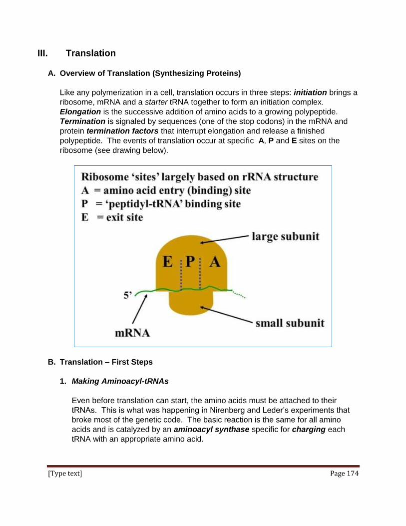
[Type text] Page 174

III. Translation

A. Overview of Translation (Synthesizing Proteins)

Like any polymerization in a cell, translation occurs in three steps: initiation brings a

ribosome, mRNA and a starter tRNA together to form an initiation complex.

Elongation is the successive addition of amino acids to a growing polypeptide.

Termination is signaled by sequences (one of the stop codons) in the mRNA and

protein termination factors that interrupt elongation and release a finished

polypeptide. The events of translation occur at specific A, P and E sites on the

ribosome (see drawing below).

B. Translation – First Steps

1. Making Aminoacyl-tRNAs

Even before translation can start, the amino acids must be attached to their

tRNAs. This is what was happening in Nirenberg and Leder’s experiments that

broke most of the genetic code. The basic reaction is the same for all amino

acids and is catalyzed by an aminoacyl synthase specific for charging each

tRNA with an appropriate amino acid.

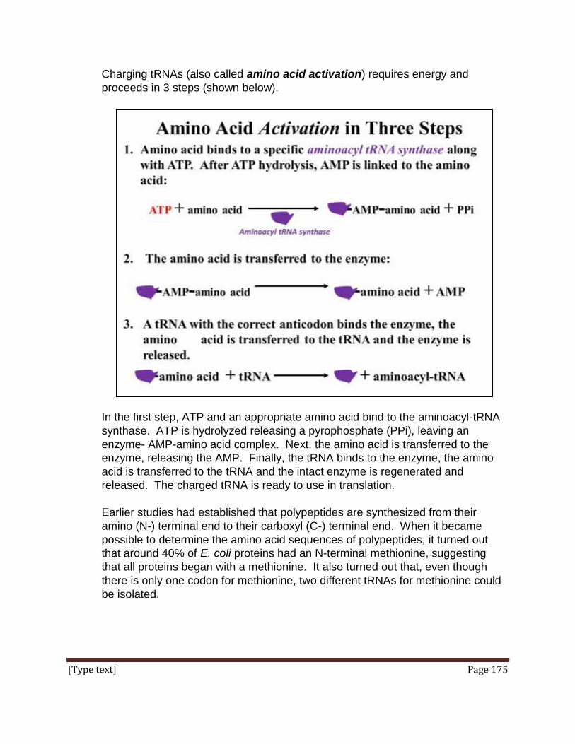
[Type text] Page 175

Charging tRNAs (also called amino acid activation) requires energy and

proceeds in 3 steps (shown below).

In the first step, ATP and an appropriate amino acid bind to the aminoacyl-tRNA

synthase. ATP is hydrolyzed releasing a pyrophosphate (PPi), leaving an

enzyme- AMP-amino acid complex. Next, the amino acid is transferred to the

enzyme, releasing the AMP. Finally, the tRNA binds to the enzyme, the amino

acid is transferred to the tRNA and the intact enzyme is regenerated and

released. The charged tRNA is ready to use in translation.

Earlier studies had established that polypeptides are synthesized from their

amino (N-) terminal end to their carboxyl (C-) terminal end. When it became

possible to determine the amino acid sequences of polypeptides, it turned out

that around 40% of E. coli proteins had an N-terminal methionine, suggesting

that all proteins began with a methionine. It also turned out that, even though

there is only one codon for methionine, two different tRNAs for methionine could

be isolated.

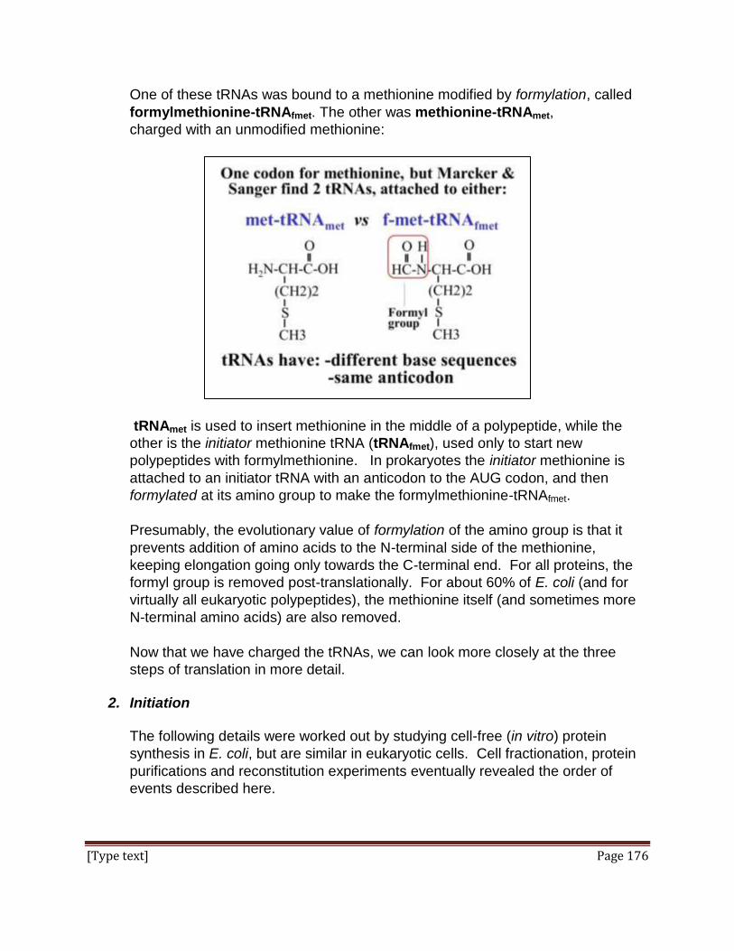
[Type text] Page 176

One of these tRNAs was bound to a methionine modified by formylation, called

formylmethionine-tRNAfmet. The other was methionine-tRNAmet,

charged with an unmodified methionine:

tRNAmet is used to insert methionine in the middle of a polypeptide, while the

other is the initiator methionine tRNA (tRNAfmet), used only to start new

polypeptides with formylmethionine. In prokaryotes the initiator methionine is

attached to an initiator tRNA with an anticodon to the AUG codon, and then

formylated at its amino group to make the formylmethionine-tRNAfmet.

Presumably, the evolutionary value of formylation of the amino group is that it

prevents addition of amino acids to the N-terminal side of the methionine,

keeping elongation going only towards the C-terminal end. For all proteins, the

formyl group is removed post-translationally. For about 60% of E. coli (and for

virtually all eukaryotic polypeptides), the methionine itself (and sometimes more

N-terminal amino acids) are also removed.

Now that we have charged the tRNAs, we can look more closely at the three

steps of translation in more detail.

2. Initiation

The following details were worked out by studying cell-free (in vitro) protein

synthesis in E. coli, but are similar in eukaryotic cells. Cell fractionation, protein

purifications and reconstitution experiments eventually revealed the order of

events described here.

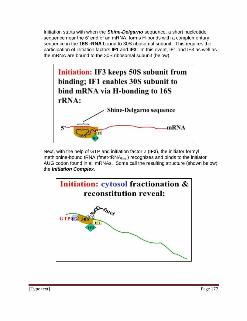
[Type text] Page 177

Initiation starts with when the Shine-Delgarno sequence, a short nucleotide

sequence near the 5’ end of an mRNA, forms H-bonds with a complementary

sequence in the 16S rRNA bound to 30S ribosomal subunit. This requires the

participation of initiation factors IF1 and IF3. In this event, IF1 and IF3 as well as

the mRNA are bound to the 30S ribosomal subunit (below).

Next, with the help of GTP and initiation factor 2 (IF2), the initiator formyl

methionine-bound tRNA (fmet-tRNAfmet) recognizes and binds to the initiator

AUG codon found in all mRNAs. Some call the resulting structure (shown below)

the Initiation Complex.

[Type text] Page 178

In the last step of initiation, the large ribosomal subunit binds to this complex,

with the concurrent disassociation of the initiation factors. The initiator fmet-

tRNAfmet ends up in the P site of the ribosome. Some prefer to call the structure

formed at this point the Initiation Complex (below).

The sequence of steps in Initiation is animated at the links below:

Small subunit binds mRNA: http://youtu.be/0m-PXfWWxNA

Formation of an initiation complex: http://youtu.be/KoU9y3W3wsk

In the next steps, look for the entry of a second aa-tRNAaa into an amino acid

entry site on the ribosome. These events will start the polypeptide elongation

process.

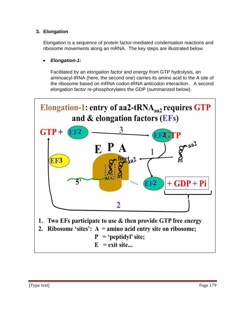
[Type text] Page 179

3. Elongation

Elongation is a sequence of protein factor-mediated condensation reactions and

ribosome movements along an mRNA. The key steps are illustrated below.

Elongation-1:

Facilitated by an elongation factor and energy from GTP hydrolysis, an

aminoacyl-tRNA (here, the second one) carries its amino acid to the A site of

the ribosome based on mRNA codon-tRNA anticodon interaction. A second

elongation factor re-phosphorylates the GDP (summarized below).

2

3

-

2

2

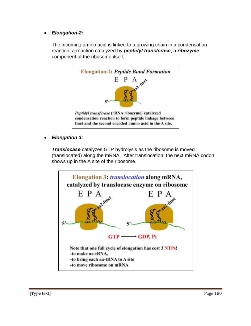
[Type text] Page 180

Elongation-2:

The incoming amino acid is linked to a growing chain in a condensation

reaction, a reaction catalyzed by peptidyl transferase, a ribozyme

component of the ribosome itself.

Elongation 3:

Translocase catalyzes GTP hydrolysis as the ribosome is moved

(translocated) along the mRNA. After translocation, the next mRNA codon

shows up in the A site of the ribosome.

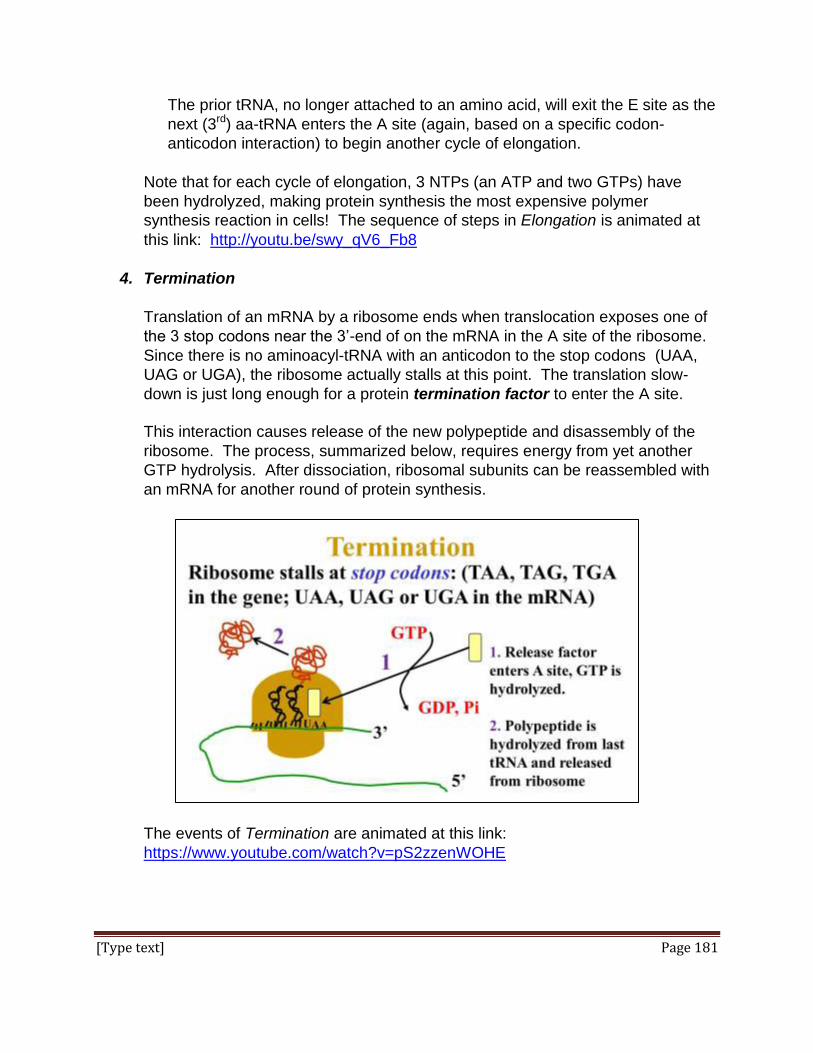
[Type text] Page 181

The prior tRNA, no longer attached to an amino acid, will exit the E site as the

next (3rd) aa-tRNA enters the A site (again, based on a specific codon-

anticodon interaction) to begin another cycle of elongation.

Note that for each cycle of elongation, 3 NTPs (an ATP and two GTPs) have

been hydrolyzed, making protein synthesis the most expensive polymer

synthesis reaction in cells! The sequence of steps in Elongation is animated at

this link: http://youtu.be/swy_qV6_Fb8

4. Termination

Translation of an mRNA by a ribosome ends when translocation exposes one of

the 3 stop codons near the 3’-end of on the mRNA in the A site of the ribosome.

Since there is no aminoacyl-tRNA with an anticodon to the stop codons (UAA,

UAG or UGA), the ribosome actually stalls at this point. The translation slow-

down is just long enough for a protein termination factor to enter the A site.

This interaction causes release of the new polypeptide and disassembly of the

ribosome. The process, summarized below, requires energy from yet another

GTP hydrolysis. After dissociation, ribosomal subunits can be reassembled with

an mRNA for another round of protein synthesis.

The events of Termination are animated at this link:

https://www.youtube.com/watch?v=pS2zzenWOHE

[Type text] Page 182

Two final notes about translation:

1. Multiple ribosomes can translate the an mRNA at the same time, forming a

polyribosome, or polysome for short (see Ch. 1).

2. We have seen some examples of post-translational processing. Most proteins,

especially in eukaryotes, undergo one or more additional steps of post-translational

processing before becoming biologically active. We’ll see more examples in

upcoming chapters.

Some iText & VOP Key Words and Terms

64 codons genetic code ribonucleoprotein

adapter molecules initiation ribosome

amino terminus initiation complex small ribosomal subunit

aminoacyl tRNA initiation factors start codon

aminoacyl tRNA synthase initiator tRNA stop codons

amino acid attachment site large ribosomal subunit termination

anticodon meaningful codons termination factor

AUG mRNA, tRNA translocation

bacterial bound ribosomes nascent chains triplets

carboxy terminus ochre, amber, opal tRNA v. tRNAaa

colinearity peptide linkage UAG, UUA, UGA

comma-less genetic code peptidyl transferase universal genetic code

degenerate genetic code polypeptide UUU

elongation polysome Wobble Hypothesis

free v. bound ribosomes reading phase

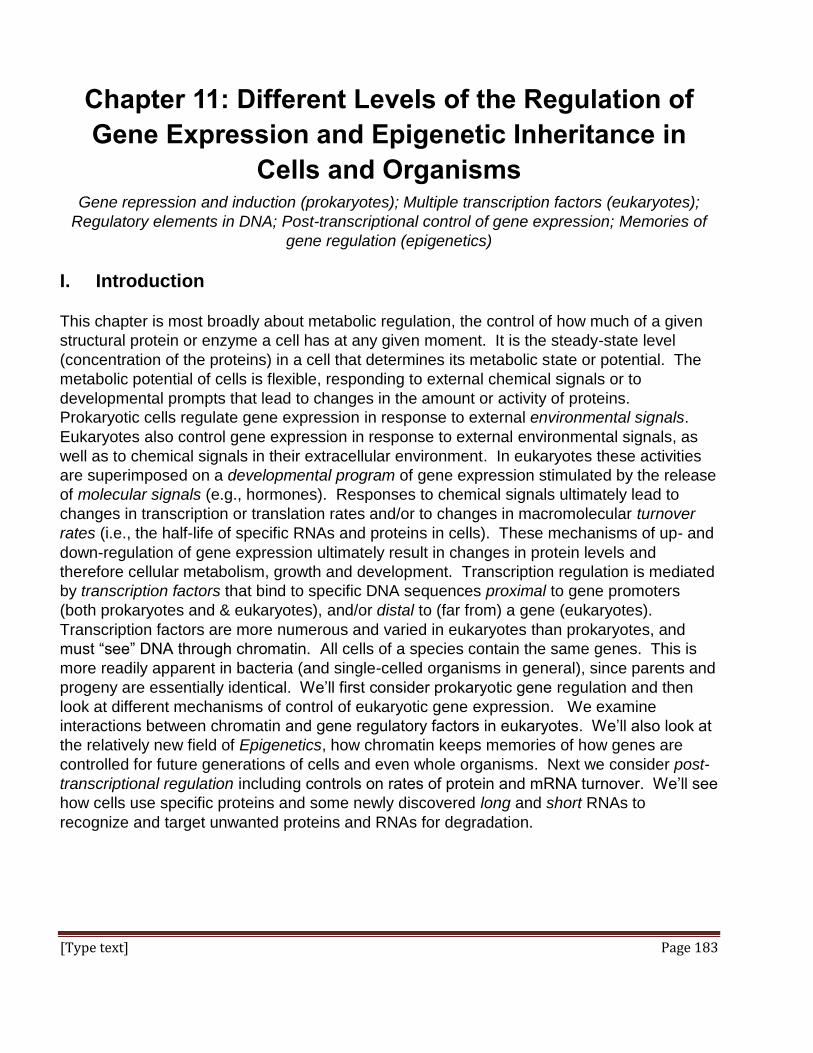
[Type text] Page 183

Chapter 11: Different Levels of the Regulation of

Gene Expression and Epigenetic Inheritance in

Cells and Organisms Gene repression and induction (prokaryotes); Multiple transcription factors (eukaryotes);

Regulatory elements in DNA; Post-transcriptional control of gene expression; Memories of

gene regulation (epigenetics)

I. Introduction

This chapter is most broadly about metabolic regulation, the control of how much of a given

structural protein or enzyme a cell has at any given moment. It is the steady-state level

(concentration of the proteins) in a cell that determines its metabolic state or potential. The

metabolic potential of cells is flexible, responding to external chemical signals or to

developmental prompts that lead to changes in the amount or activity of proteins.

Prokaryotic cells regulate gene expression in response to external environmental signals.

Eukaryotes also control gene expression in response to external environmental signals, as

well as to chemical signals in their extracellular environment. In eukaryotes these activities

are superimposed on a developmental program of gene expression stimulated by the release

of molecular signals (e.g., hormones). Responses to chemical signals ultimately lead to

changes in transcription or translation rates and/or to changes in macromolecular turnover

rates (i.e., the half-life of specific RNAs and proteins in cells). These mechanisms of up- and

down-regulation of gene expression ultimately result in changes in protein levels and

therefore cellular metabolism, growth and development. Transcription regulation is mediated

by transcription factors that bind to specific DNA sequences proximal to gene promoters

(both prokaryotes and & eukaryotes), and/or distal to (far from) a gene (eukaryotes).

Transcription factors are more numerous and varied in eukaryotes than prokaryotes, and

must “see” DNA through chromatin. All cells of a species contain the same genes. This is

more readily apparent in bacteria (and single-celled organisms in general), since parents and

progeny are essentially identical. We’ll first consider prokaryotic gene regulation and then

look at different mechanisms of control of eukaryotic gene expression. We examine

interactions between chromatin and gene regulatory factors in eukaryotes. We’ll also look at

the relatively new field of Epigenetics, how chromatin keeps memories of how genes are

controlled for future generations of cells and even whole organisms. Next we consider post-

transcriptional regulation including controls on rates of protein and mRNA turnover. We’ll see

how cells use specific proteins and some newly discovered long and short RNAs to

recognize and target unwanted proteins and RNAs for degradation.

[Type text] Page 184

Voice-Over PowerPoint Presentations

Gene Regulation in Prokaryotes VOP

Gene Regulation in Eukaryotes VOP

Gene Activity & Chromatin VOP

Epigenetic Inheritance

(Post-Transcriptional Regulation)

Learning Objectives

When you have mastered the information in this chapter and the associated VOPs, you

should be able to:

1. compare and contrast transcription factors and so-called cis-acting elements.

2. articulate the role of DNA bending in the regulation of gene expression.

3. explain the benefits of bacterial operon regulation.

4. explain why all bacterial genes are not organized into operons.

5. compare and contrast regulation of the lac and trp operons in E. coli.

6. compare and contrast regulatory genes and structural genes in E. coli.

7. discuss why a 4th gene was suspected in lac operon regulation.

8. distinguish between repression and de-repression and between positive and negative

regulation, using examples. For example, explain how it is possible to have repression by

positive regulation.

9. draw and label prokaryotic and eukaryotic genes for a protein, with all functional regions..

10. compare and contrast several different mechanisms of gene regulation in eukaryotic cells.

11. describe the transcription initiation complex of a regulated gene in eukaryotes.

12. As you would define them, articulate any differences between gene expression and

transcription regulation.

13. define a gene.

14. distinguish between the roles of enhancers and other cis-acting elements in transcription

regulation.

15. compare and contrast the genome and the epigenome.

16. compare and contrast the origins and functions of miRNA and siRNA.

17. describe the main mechanisms for degrading unwanted proteins in eukaryotic cells and

speculate on how bacteria might accomplish the same task.

II. Gene Regulation in Prokaryotes

Many prokaryotic genes are organized as operons, linked genes that are transcribed into a

single mRNA encoding 2 or more proteins. Operons usually encode proteins with related

functions. By regulating the activity of an operon, amounts of their encoded proteins can be

coordinately controlled. Genes for enzymes or other proteins whose expression must be

[Type text] Page 185

controlled are called structural genes while those that encode proteins that bind DNA to

control gene expression are called regulatory genes. The lac operon of E. coli is an example.

The polycistronic mRNA transcript is simultaneously translated into each of the proteins

encoded in the operon, as shown below (and described at http://youtu.be/YN3qUL5svnQ).

Regulation of an operon (or of an individual gene for that matter) can be by repression or by

induction. If an operon is active unless inhibited by a repressor it is a repressible operon. If

the operon is inactive but can be induced by a small molecule, it is called an inducible

operon. Induction or repression can occur when such a molecule binds to an inducer protein

that then binds to DNA near the gene causing it to be transcribed, causing it to be

transcribed. The kicker is that the molecule might instead induce transcription by de-

repression. Here a small molecule binds repressor protein, causing it to come off the DNA

near the gene. In both cases, the small molecules are intracellular metabolites that reflect

the metabolic status of the cell and thus the gene(s) that needs to be activated or silenced.

The lac and trp operons are good examples of bacterial gene regulation. The lac operon is

regulated by induction by de-repression as well as by a positive inducer. The operon is also

controlled by a process called inducer exclusion (see below). The trp operon is regulated by

repression by a repressor protein. We’ll look at the regulation of both operons in detail

below.

[Type text] Page 186

A. Mechanisms of Control of the lac Operon

In the animal digestive tract (including ours), genes of the E. coli lac operon regulate the

use of lactose as an alternative nutrient to glucose. Think of eating cheese instead of

chocolate. The operon consists of three structural genes, lacZ, lacY, and lacA.

Structural genes in bacteria are to be distinguished from regulatory genes. While both

kinds of genes encode proteins, the regulatory genes encode proteins whose function is

to bind to DNA and regulate the structural genes! The operon is transcribed into a

multigene transcript (illustrated below). The basics of lac operon transcription are

(silently!) animated at http://youtu.be/RKf66-VzYI0.

Since the preferred nutrient for E. coli is glucose, the cells will only use lactose as an

alternative energy and carbon source if glucose levels in the environment are limiting.

When glucose levels are low and lactose is available, the operon is transcribed and the 3

enzyme products are translated. The lacZ gene encodes β-galactosidase, the enzyme

that breaks lactose (a disaccharide) into galactose and glucose. The lacY gene encodes

lactose permease, a membrane protein that facilitates lactose entry into the cells. The

role of the lacA gene (a transacetylase) in lactose energy metabolism is not well

understood. The lac operon is regulated by derepression as well as direct induction,

leading to transcription of the lac genes only when necessary (i.e., in the presence of

lactose and absence of glucose).

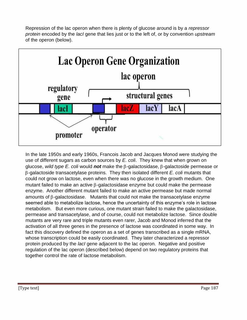
[Type text] Page 187

Repression of the lac operon when there is plenty of glucose around is by a repressor

protein encoded by the lacI gene that lies just or to the left of, or by convention upstream

of the operon (below).

In the late 1950s and early 1960s, Francois Jacob and Jacques Monod were studying the

use of different sugars as carbon sources by E. coli. They knew that when grown on

glucose, wild type E. coli would not make the -galactosidase, -galactoside permease or

-galactoside transacetylase proteins. They then isolated different E. coli mutants that

could not grow on lactose, even when there was no glucose in the growth medium. One

mutant failed to make an active -galactosidase enzyme but could make the permease

enzyme. Another different mutant failed to make an active permease but made normal

amounts of -galactosidase. Mutants that could not make the transacetylase enzyme

seemed able to metabolize lactose, hence the uncertainty of this enzyme’s role in lactose

metabolism. But even more curious, one mutant strain failed to make the galactosidase,

permease and transacetylase, and of course, could not metabolize lactose. Since double

mutants are very rare and triple mutants even rarer, Jacob and Monod inferred that the

activation of all three genes in the presence of lactose was coordinated in some way. In

fact this discovery defined the operon as a set of genes transcribed as a single mRNA,

whose transcription could be easily coordinated. They later characterized a repressor

protein produced by the lacI gene adjacent to the lac operon. Negative and positive

regulation of the lac operon (described below) depend on two regulatory proteins that

together control the rate of lactose metabolism.

[Type text] Page 188

1. Negative Regulation of the lac Operon – Repression and De-repression

Refer to the illustration below to identify the players in lac operon induction.

The first control mechanism involves a regulatory repressor protein called the lactose

repressor (#12, #7). The lacI gene (# 2) coding for the repressor protein lies

upstream of the lac operon and is always expressed (such unregulated genes are

called constitutive). In the absence of lactose in the growth medium, the repressor

protein binds very tightly to a short DNA sequence called the lac operator (#6) just

downstream of the promoter (#4) the near the start of the lacZ gene. This binding

interferes with binding of RNA polymerase (#5) to the promoter and its forward

movement. Under these conditions, transcription of the lacZ, lacY and lacA genes

(#s 8, 9 & 10) occurs at very low levels. But when cells are grown in the presence of

lactose, a lactose metabolite called allolactose (#13) is formed in the cell. Allolactose

binds to the repressor sitting on the operator DNA (a 2-part complex shown as #7),

causing a change in its shape. Thus altered, the repressor dissociates from the

operator and the RNA polymerase is able to transcribe the lac operon genes, thereby

leading to higher levels of the encoded proteins.

Activation of the lac operon by allolactose-mediated derepression is shown in the

animation at the following link: http://youtu.be/MNQ8CzhDfCg

[Type text] Page 189

2. Induction of the lac Operon

The second control mechanism regulating lac operon expression is mediated by the

cAMP-bound catabolite activator protein, also called the cAMP receptor protein, or

CAP. When glucose is available, cellular levels of cAMP are low in the cells and CAP

is in an inactive conformation. But if glucose is absent or its levels are low, cAMP

levels rise and cAMP binds to the CAP. In its active conformation, CAP binds to the

operon where it actually causes DNA to bend (below).

Bending the double helix loosens H-bonds, thus facilitating RNA polymerase binding

and transcription initiation. If lactose is available, transcription of the lac genes is

maximally induced by negative control (de-repression by allolactose) and positive

control (by cAMP-bound CAP).

In recent years, additional layers of lac operon have been uncovered. In one case,

the ability of lac permease in the cell membrane to transport lactose is regulated. In

another case, additional operator sequences have been discovered that play a role in

operon regulation.

3. Regulation of Lactose use by Inducer Exclusion

When glucose levels are high (even in the presence of lactose) phosphate is

consumed to phosphorylate glycolytic intermediates, keeping cytoplasmic phosphate

levels low. Under these conditions, unphosphorylated EIIAGlc binds to the lactose

permease enzyme in the cell membrane, preventing it from bringing lactose into the

cell. On the other hand, if glucose levels are low in the growth medium, phosphate

concentrations in the cells rise sufficiently for specific kinases to phosphorylate the

EIIAGlc. Phosphorylated EIIAGlc then undergoes an allosteric change and dissociates

from the lactose permease, making it active so that more lactose can enter the cell.

[Type text] Page 190

Glucose is normally transported into the cell by a phosphoenolpyruvate (PEP)-

dependent phosphotransferase system (PTS). PTS is a phosphorylation cascade

that is activated when glucose levels are low, and the last kinase in the cascade would

act to phosphorylate EIIAGlc. High glucose levels blocking lactose entry into the cells,

effectively preventing allolactose formation and the derepression of the lac operon.

4. Repressor Protein Structure and Additional Operator Sequences!

The lac repressor is a tetramer of identical subunits (below) and each subunit contains

a helix-turn-helix motif capable of binding to DNA.

However, the operator DNA sequence consists of a pair of inverted repeats spaced

apart in such a way that they can only interact two of the repressor subunits, leaving

the function of the other two subunits unknown… that is, until recently…!

Two more operator regions were recently characterized in the lac operon. One, called

O2, is within the lac z gene itself and the other, called O3, lies near the end but within

the lac I gene. Apart from their unusual location within actual genes, these operators,

which interact with the remaining two repressor subunits, remained undetected

because mutations in the O2 or the O3 region individually do not contribute

substantially to the effect of lactose in derepressing the lac operon. Only if both

regions are mutated at the same time is a substantial reduction in binding of the

repressor to the operon.

From: http://en.wikipedia.org/wiki/Lac_repressor

[Type text] Page 191

B. Mechanism of Control of the Tryptophan Operon

If ample tryptophan (trp) is available, the tryptophan synthesis pathway can be inhibited

in two ways. First, recall how feedback inhibition by excess tryptophan can allosterically

inhibit the trp synthesis pathway. A rapid response occurs when tryptophan is present in

excess, resulting in feedback inhibition by blocking the first of 5 enzymes in the

tryptophan synthesis pathway. The polypeptides that make up two of these enzymes are

encoded by the trp operon.

Enzyme 1 is a multimeric protein is made from polypeptides encoded by the trp5 and trp4

genes. Enzyme 3 is made up of the trp1 and trp2 gene products. When tryptophan

levels are low because the amino acid is being consumed (e.g. in protein synthesis), E.

coli cells will continue to synthesize the amino acid (illustrated below):

On the other hand, if the environment is high in tryptophan, or if the cell slows down its

use of the amino acid, trp accumulates in the cytoplasm where it will bind to the trp

repressor.

Active Transcription

translation of 5 polypeptides

[Type text] Page 192

In its altered shape, the trp-bound repressor can bind to the trp operon operator sequence

and block RNA polymerase from transcribing the operon, as shown below:

In this scenario, tryptophan is described as a co-repressor.

III. Gene Regulation in Eukaryotes

A. The Difference between Eukaryotic and Prokaryotic Gene Regulation

Every cell in any multicellular eukaryotic organism contains the same DNA (genes) as

every other cell. Here is the proof:

[Type text] Page 193

Therefore what makes one cell type different from another is which set of genes is

expressed in each. Looked at another way, different cells contain different sets of

proteins. The cells can control their metabolic state by controlling how much of each

protein they make at a given moment. This accounts for how cells with the same genetic

makeup can produce a different set of gene products and look and function so differently.

Compared to prokaryotes, eukaryotes have many steps between transcription of an

mRNA and the accumulation of a polypeptide end-product. 11 of these steps are shown

in the pathway of eukaryotic gene regulation below.

Theoretically, cells could regulate any one or multiple steps in this process, thereby

affecting the steady state concentration of a polypeptide in the cells. While regulation of

any of these steps is possible, the expression of a single gene is not typically controlled at

more than a few steps. A common form of gene regulation is at the level of transcription

initiation, turning genes on or off, similar to transcriptional control in bacteria.

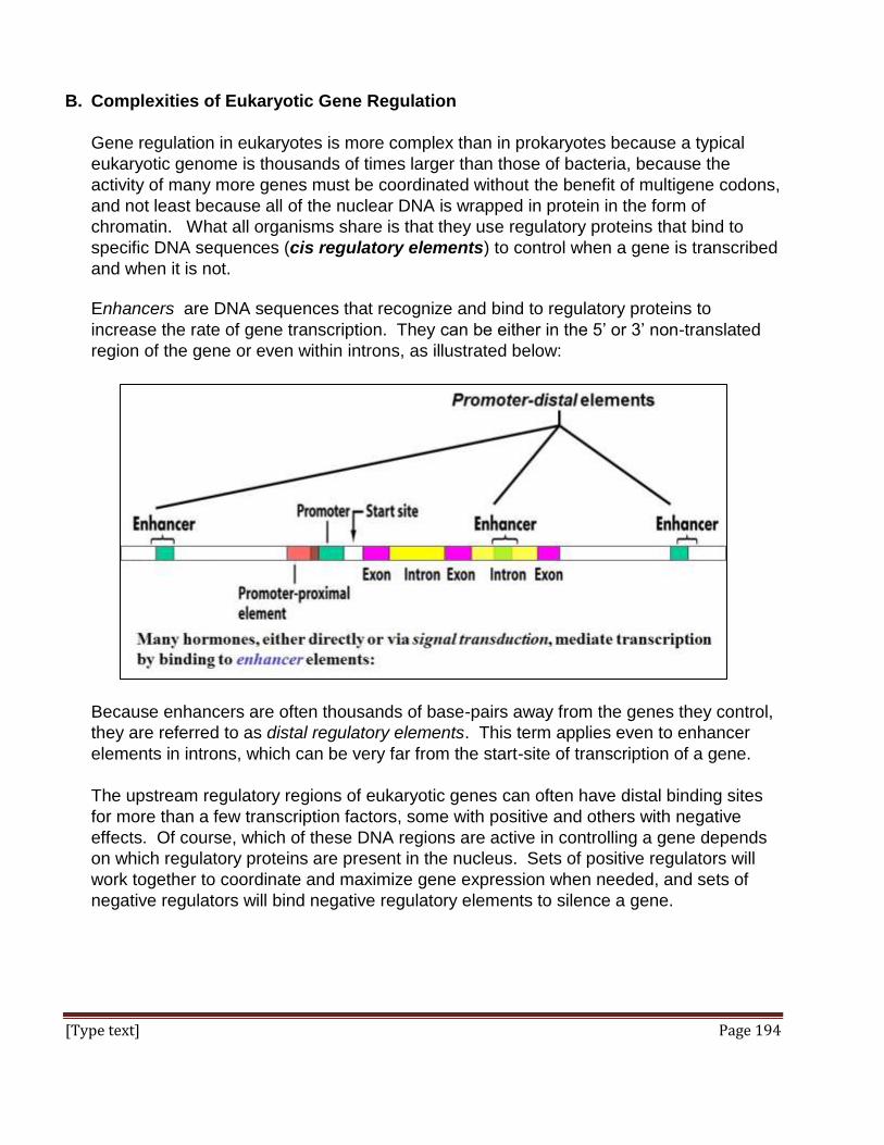
[Type text] Page 194

B. Complexities of Eukaryotic Gene Regulation

Gene regulation in eukaryotes is more complex than in prokaryotes because a typical

eukaryotic genome is thousands of times larger than those of bacteria, because the

activity of many more genes must be coordinated without the benefit of multigene codons,

and not least because all of the nuclear DNA is wrapped in protein in the form of

chromatin. What all organisms share is that they use regulatory proteins that bind to

specific DNA sequences (cis regulatory elements) to control when a gene is transcribed

and when it is not.

Enhancers are DNA sequences that recognize and bind to regulatory proteins to

increase the rate of gene transcription. They can be either in the 5’ or 3’ non-translated

region of the gene or even within introns, as illustrated below:

Because enhancers are often thousands of base-pairs away from the genes they control,

they are referred to as distal regulatory elements. This term applies even to enhancer

elements in introns, which can be very far from the start-site of transcription of a gene.

The upstream regulatory regions of eukaryotic genes can often have distal binding sites

for more than a few transcription factors, some with positive and others with negative

effects. Of course, which of these DNA regions are active in controlling a gene depends

on which regulatory proteins are present in the nucleus. Sets of positive regulators will

work together to coordinate and maximize gene expression when needed, and sets of

negative regulators will bind negative regulatory elements to silence a gene.

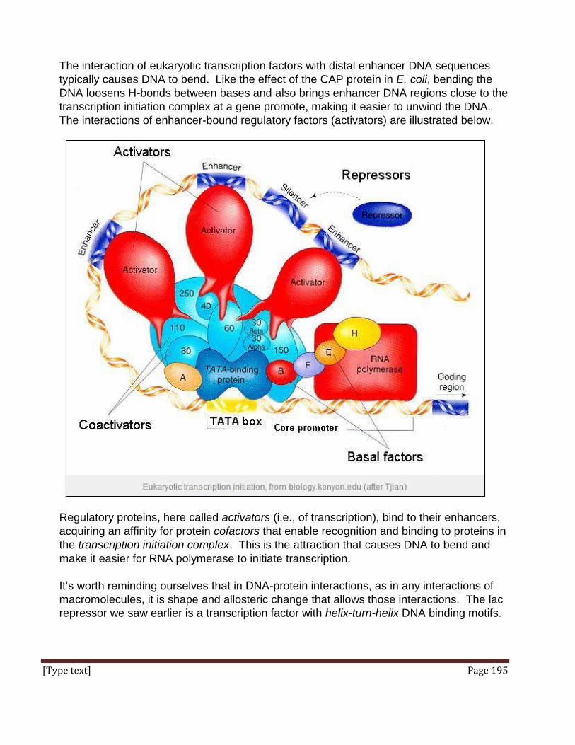
[Type text] Page 195

The interaction of eukaryotic transcription factors with distal enhancer DNA sequences

typically causes DNA to bend. Like the effect of the CAP protein in E. coli, bending the

DNA loosens H-bonds between bases and also brings enhancer DNA regions close to the

transcription initiation complex at a gene promote, making it easier to unwind the DNA.

The interactions of enhancer-bound regulatory factors (activators) are illustrated below.

Regulatory proteins, here called activators (i.e., of transcription), bind to their enhancers,

acquiring an affinity for protein cofactors that enable recognition and binding to proteins in

the transcription initiation complex. This is the attraction that causes DNA to bend and

make it easier for RNA polymerase to initiate transcription.

It’s worth reminding ourselves that in DNA-protein interactions, as in any interactions of

macromolecules, it is shape and allosteric change that allows those interactions. The lac

repressor we saw earlier is a transcription factor with helix-turn-helix DNA binding motifs.

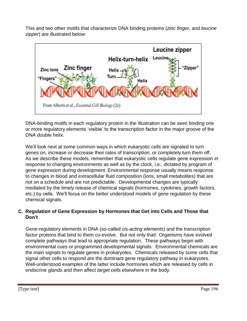
[Type text] Page 196

This and two other motifs that characterize DNA binding proteins (zinc finger, and leucine

zipper) are illustrated below:

DNA-binding motifs in each regulatory protein in the illustration can be seen binding one

or more regulatory elements ‘visible’ to the transcription factor in the major groove of the

DNA double helix.

We’ll look next at some common ways in which eukaryotic cells are signaled to turn

genes on, increase or decrease their rates of transcription, or completely turn them off.

As we describe these models, remember that eukaryotic cells regulate gene expression in

response to changing environments as well as by the clock, i.e., dictated by program of

gene expression during development. Environmental response usually means response

to changes in blood and extracellular fluid composition (ions, small metabolites) that are

not on a schedule and are not predictable. Developmental changes are typically

mediated by the timely release of chemical signals (hormones, cytokines, growth factors,

etc.) by cells. We’ll focus on the better understood models of gene regulation by these

chemical signals.

C. Regulation of Gene Expression by Hormones that Get into Cells and Those that

Don’t

Gene-regulatory elements in DNA (so-called cis-acting elements) and the transcription

factor proteins that bind to them co-evolve. But not only that! Organisms have evolved

complete pathways that lead to appropriate regulation. These pathways begin with

environmental cues or programmed developmental signals. Environmental chemicals are

the main signals to regulate genes in prokaryotes. Chemicals released by some cells that

signal other cells to respond are the dominant gene regulatory pathway in eukaryotes.

Well-understood examples of the latter include hormones which are released by cells in

endocrine glands and then affect target cells elsewhere in the body.

[Type text] Page 197

1. How Steroid Hormones Regulate Transcription

Steroid hormones cross the cell membranes to have their effects. Common ones are

testosterone, estrogens, progesterone, glucocorticoids and mineral corticoids. Once

in the cytoplasm, steroid hormones bind to a receptor protein to form a steroid

hormone-receptor complex that can enter the nucleus and bind to those cis-acting

regulatory elements (typically DNA sequences that function as enhancers, but also as

silencers). The basic events are illustrated below.

Here the steroid (the triangle) enters the cell. When binding to the steroid hormone

receptor (shown as blue and black polypeptide subunits in the cytoplasm), there is a

conformational change in the receptor and the ‘black’ protein subunit dissociates from

the hormone-receptor complex, which then enters the nucleus. The black protein is

called Hsp90, or heat shock protein 90, a protein of 90,000Da molecular weight. Note

that receptors for some steroid hormones are resident in the nucleus, but the basic

mechanism of action is quite similar.

The fascinating thing about Hsp90 and other heat shock proteins is that they were

originally discovered in cells subjected to heat stress. When the temperature gets

high enough, cells shut down most transcription and make instead special heat shock

[Type text] Page 198

transcripts and proteins. These proteins seem to protect the cells against metabolic

damage until temperatures return to normal. Since most cells never experience such

high temperatures, the evolutionary significance of this protective mechanism and of

the existence of heat shock proteins was unclear. But as we can see, heat shock

proteins do in fact have critical cellular functions, in this case blocking the DNA-

binding site of the hormone receptor until a specific steroid hormone binds to it.

Back to hormone action! No longer associated with the Hsp90 protein, the receptor

bound to its hormone cofactor binds to a transcription control element (a nucleotide

sequence cis element) in the DNA, turning transcription of a gene on or off. The

process is animated here: http://youtu.be/G590s9xZ9VA. The hormone receptors for

some steroid hormones are already in the nucleus of the cell, so the hormone has to

cross the plasma membrane and the nuclear envelope to access the receptor.

In looking at glycolysis and respiration (energy metabolism), we saw that

glucocorticoids turn on the genes of gluconeogenesis. Among other things, steroid

hormones control sexual development and reproductive cycling in females, salt and

mineral homeostasis in the blood, metamorphosis in arthropods, etc…, all by

regulating gene expression.

2. How Protein Hormones Regulate Transcription

Protein hormones are of course large and soluble, with highly charged surfaces.

Therefore they can’t cross the phospholipid membrane barrier to get into cells. To

have any effect at all, they must bind to receptors on the surface of cells. These

receptors are typically membrane glycoproteins. The information (signals) carried by

protein hormones must be conveyed into the cell indirectly. This process is called

signal transduction.

There are two well-known pathways of signal transduction, each of which involves

activating pathways of protein phosphorylation in cytoplasm that eventually results in

activation of a transcription factor that binds to regulatory DNA and either turns a gene

on or off.

Some protein hormones bind to cell membrane receptors that after undergoing

allosteric change, activates other membrane proteins. The net effect is to increase

intracellular concentrations of a cytoplasmic 2nd messenger, shown in the drawing

below as cAMP. cAMP mediates many hormonal responses, controlling both gene

activity and enzyme activity. In this case, cAMP binds to a protein kinase, the first of

several in a pathway (called a phosphorylation cascade).

[Type text] Page 199

The last in the series of proteins to be phosphorylated is an activated transcription

factor that can turn on a gene (below).

The other kind of signal transduction, shown below, involves a hormone receptor that

is itself a protein kinase (below).

[Type text] Page 200

Binding of the signal protein (e.g. hormone) to this kind receptor causes an allosteric

change that activates the kinase, starting phosphorylation cascade resulting in an

active transcription factor.

These two kinds of signal transduction are animated at this link:

http://youtu.be/CSvNSm7pqyc

We’ll be looking at signal transduction in greater detail in a later chapter.

IV. Regulating Eukaryotic Genes Means Contending with Chromatin

Consider again the illustration of the different levels of chromatin structure (below).

Transcription factors bind specific DNA sequences by detecting them through the grooves

(mainly the major groove) in the double helix. But the drawing above reminds us that unlike

the nearly naked DNA of bacteria, eukaryotic (nuclear) DNA is dressed with proteins that in

aggregate are greater than the mass of the DNA they cover. The protein-DNA complex of

the genome is of course, chromatin.

1

2

3

[Type text] Page 201

DNA coated with histone proteins forma a 9 nm diameter beads on a string necklace-like

structure, in which the beads are called nucleosomes. The association of specific non-

histone proteins causes the nucleosomes to fold over on themselves to form the 30 nm

solenoid. Further accretion of non-histone proteins leads to more folding and the formation

of the euchromatin and heterochromatin characteristic of chromatin in non-dividing cells.

In dividing cells, the chromatin is further condensed to form the chromosomes that will be

separated during either mitosis or meiosis.

As we saw earlier, it is possible to selectively extract chromatin. Take a second look at the

results of a typical extraction of chromatin from isolated nuclei below.

Recall that biochemical analysis of the 10 nm filament (nucleosome) extract revealed that the

DNA was wrapped around histone protein octamers, the nucleosomes or beads in this

beads-on-a-string structure. The histone proteins are highly conserved in the evolution of

eukaryotes (they are not found in prokaryotes). They are also very basic (many lysine and

arginine residues) and therefore very positively charged. This explains why they seem to

arrange themselves uniformly along DNA, binding to the negatively charged phosphodiester

backbone of DNA in the double helix.

[Type text] Page 202

Experiments in which total nuclear chromatin extracts were isolated and treated with the

enzyme deoxyribonuclease (DNAse) revealed that the DNA in active genes was degraded

more rapidly than non-transcribed DNA. The interpretation is that active genes are more

accessible to DNAse because they are in chromatin that is less coiled, less condensed. DNA

in more condensed chromatin is surrounded by more proteins and therefore less accessible

to the enzyme. Thus the proteins in the more coiled DNA protect the DNA from DNAse

attack. Genes packed up in chromosomes are of course inactive. Therefore regulating gene

transcription must involve changing the shape of chromatin (chromatin remodeling) in order

to silence some genes and activate others.

Changing chromatin conformation involves chemical modification of chromatin proteins and

DNA. For example, chromatin can be modified by histone acetylation de-acetylation,

methylation and phosphorylation, reactions catalyzed by histone acetyltransferases (HAT

enzymes), de-acetylases, methyl transferases and kinases, respectively.

Nucleosomes themselves can be moved, slid and otherwise repositioned by ATP-dependent

complexes that hydrolyze ATP for energy to accomplish the physical shifts. Some cancers

are associated with mutations in genes for proteins involved in chromatin remodeling, no

doubt because failures of normal remodeling could adversely affect normal cell cycling and

normal replication.

V. Epigenetics (Click to see Wikipedia’s description)

Epigenetics means around or above (epi) genes. The original use of the term dates from

before we knew that DNA was the stuff of genes. The idea was that genetic information was

pretty stable. Therefore, differences between individuals with the same genes would result

from differences in environmental chemical influences on otherwise similar genes. Simply

put, genes are affected by time of life as well as by how and where an individual organism

lives. The term epigenetic has the same meaning today, except that we know that DNA is

the stuff of genes, and that genes are indeed influenced by the chemicals around them.

The field of epigenetics looks at protein interactions in eukaryotes that affect gene

expression. These interactions change the structure NOT of genes (or DNA), but of the

proteins (and other molecules) that affect how DNA and genes are used. As we have seen,

the control of transcription involves transcription factors that recognize and bind to regulatory

sequences in DNA such as enhancers or silencers. These protein-DNA interactions often

require selective structural changes in the conformation of the chromatin surrounding genes.

These changes can be profound, stable and not easily undone.

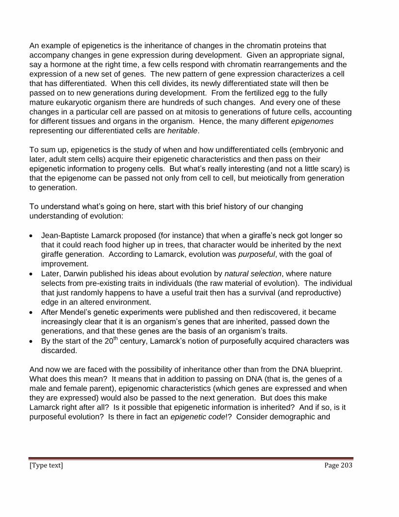
[Type text] Page 203

An example of epigenetics is the inheritance of changes in the chromatin proteins that

accompany changes in gene expression during development. Given an appropriate signal,

say a hormone at the right time, a few cells respond with chromatin rearrangements and the

expression of a new set of genes. The new pattern of gene expression characterizes a cell

that has differentiated. When this cell divides, its newly differentiated state will then be

passed on to new generations during development. From the fertilized egg to the fully

mature eukaryotic organism there are hundreds of such changes. And every one of these

changes in a particular cell are passed on at mitosis to generations of future cells, accounting

for different tissues and organs in the organism. Hence, the many different epigenomes

representing our differentiated cells are heritable.

To sum up, epigenetics is the study of when and how undifferentiated cells (embryonic and

later, adult stem cells) acquire their epigenetic characteristics and then pass on their

epigenetic information to progeny cells. But what’s really interesting (and not a little scary) is

that the epigenome can be passed not only from cell to cell, but meiotically from generation

to generation.

To understand what’s going on here, start with this brief history of our changing

understanding of evolution:

Jean-Baptiste Lamarck proposed (for instance) that when a giraffe’s neck got longer so

that it could reach food higher up in trees, that character would be inherited by the next

giraffe generation. According to Lamarck, evolution was purposeful, with the goal of

improvement.

Later, Darwin published his ideas about evolution by natural selection, where nature

selects from pre-existing traits in individuals (the raw material of evolution). The individual

that just randomly happens to have a useful trait then has a survival (and reproductive)

edge in an altered environment.

After Mendel’s genetic experiments were published and then rediscovered, it became

increasingly clear that it is an organism’s genes that are inherited, passed down the

generations, and that these genes are the basis of an organism’s traits.

By the start of the 20th century, Lamarck’s notion of purposefully acquired characters was

discarded.

And now we are faced with the possibility of inheritance other than from the DNA blueprint.

What does this mean? It means that in addition to passing on DNA (that is, the genes of a

male and female parent), epigenomic characteristics (which genes are expressed and when

they are expressed) would also be passed to the next generation. But does this make

Lamarck right after all? Is it possible that epigenetic information is inherited? And if so, is it

purposeful evolution? Is there in fact an epigenetic code!? Consider demographic and

[Type text] Page 204

health record data collected by a doctor in a town in Sweden that kept meticulous harvest,

birth, illness and death records. From the data (below), it’s as if the environment was indeed

causing an acquired change in the grandparent that is passed not to one, but through two

generations… and in a sex-specific way! It looked as if environment was influencing

inheritance! The table below shows the data from the Swedish physician.

This phenomenon was subsequently demonstrated experimentally with already pregnant rats

exposed to a toxin. The rat pups born to exposed mothers suffered a variety of illnesses.

This might be expected if the toxic effects on the mother were visited on the developing pups,

for example through the placenta. But when the diseased male rat pups matured, they were

mated to females, the pups in the new litter grew up suffering the same maladies as the male

parent, even though the pregnant females in this case were NOT exposed to the toxins.

Because the original female was already pregnant when she was exposed, the germ line

cells (eggs, sperm) of her litter had not suffered mutations in utero. This could only mean

that epigenetic patterns of gene expression caused by the toxin in pup germ line cells (those

destined to become sperm & eggs) in utero were retained during growth to sexual maturity,

and were passed on to their progeny, even while gestating in a normal unexposed female.

These days, the term epigenetics is used to describe heritable changes in chromatin

modifications and gene expression. We now know that the epigenetic configurations of

chromatin that are most stable include patterns of histone modification (acetylation,

phosphorylation, methylation…) or DNA (methylation, phosphorylation…). Such changes

can convert the 30nm fiber to the 10nm ‘beads-on-a-string nucleosome necklace… and vice

versa. Such changes in chromatin (chromatin remodeling) lead to alter patterns of gene

expression, whether during normal development or when deranged by environmental factors

(abundance or limits on nutrition, toxins/poisons or other life-style choices). The active study

of DNA methylation patterns even has its own name, methylomics!

So, what is scary about epigenetic inheritance? Can you be sure that your smoking or

sugary eating habits won’t affect the health of your children or grandchildren?

[Type text] Page 205

VI. Post-transcriptional Control of Gene Expression

A. Small RNAs – miRNA and siRNA (Excerpted and adapted from The Medical

Biochemistry Page)

Not too long ago we thought that the only non-coding RNAs were tRNAs and rRNAs of

the translational machinery. But we know now that other RNAs are transcribed and that

they play various roles in gene regulation and the degradation of spent cellular DNA or

unwanted foreign DNA. Two such RNAs share some steps in their processing and

effects, albeit on different target RNA molecules.

1. Micro RNA (miRNA)

These were first discovered as small RNAs that seemed to interfere with gene

expression in C. elegans, the small flatworm that has been the subject of numerous

molecular studies of growth and development for some time now. The particular

attractions of this model organism are that it uses a genome similar in size to the

human genome (20,168 genes that code for proteins) to produce an adult worm

consisting of just 1031 cells organized into all of the major organs found in higher

organisms..., AND that it possible to trace the origins of every single cell in its body!

Here is a drawing of what little more than a thousand cells can look like in a complete

animal.

miRNAs are known to be widely distributed in all organisms where they have been

sought, where they fold into a hairpin loop when first transcribed.

[Type text] Page 206

When precursor miRNAs are first transcribed, they fold to form a hairpin loop. They

lose the loop when they are processed to make the ‘mature’ miRNA (below).

miRNAs cooperate with a protein called RISC to cause degradation of old or no-longer

needed mRNAs or mRNAs damaged during transcription. The pathway for

processing miRNAs leading to the degradation of target cellular mRNA is animated in

the following link: http://youtu.be/21C01D2Tgeg An estimated 250 miRNAs may be

sufficient to bind to diverse target RNAs.

2. Small Interfering RNA (siRNA)

siRNA was first found in plants and C. elegans (perhaps no surprise!), but like

miRNAs, siRNAs are common in many higher organisms. They were named because

they interfere with mRNAs (e.g., the transcription products of viral genomes), and the

action of siRNAs was called RNA interference (RNAi)_.. The pathway of siRNA action

during RNA interference is animated in the following link:

http://youtu.be/BTAi3RoSkV0W.

When foreign double-stranded RNAs (e.g., some viral RNA genomes) get into cells,

they are recognized as alien by a nuclease called DICER. The short double-stranded

hydrolysis products of the foreign RNA, the siRNAs, combine with RNAi Induced

Silencing Complex, or RISC proteins. The antisense SiRNA strand in the resulting

siRNA-RISC complex binds to complementary regions of foreign RNAs, targeting

them for degradation.

Custom-designed siRNAs have been used for some time to disable expression of

specific genes in order to study their function, and both miRNAs and siRNAs are being

investigated as possible therapeutic tools to inactivate genes by RNA interference,

whose expression leads to cancer or other diseases.

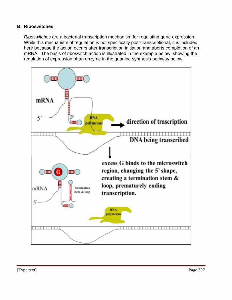
[Type text] Page 207

B. Riboswitches

Riboswitches are a bacterial transcription mechanism for regulating gene expression.

While this mechanism of regulation is not specifically post-transcriptional, it is included

here because the action occurs after transcription initiation and aborts completion of an

mRNA. The basis of riboswitch action is illustrated in the example below, showing the

regulation of expression of an enzyme in the guanine synthesis pathway below.

[Type text] Page 208

When the base guanine is at low levels in the cells, the mRNA for an enzyme in the

guanine synthesis pathway is transcribed (blue & red structure, above left). The transcript

itself folds into a a stem-&-loop structure. One of these stem-loop elements (near its 5’

end) binds gunaine when it is in excess in the cell, causing the RNA polymerase and the

partially completed mRNA to dissociate from the DNA, prematurely ending transcription.

C. Long Non-Coding RNAs

Until quite recently, we thought that only a few percent (less than 5%) of a typical

eukaryotic genome is transcribed into mRNA, with rRNAs and tRNAs making up most of

the other transcripts. And even then, only a fraction of the genome was thought to be

transcribed in any given cell. Much of the DNA between genes, and even within genes (in

the form of introns) was believed to contain junk DNA (non-descript sequences, ‘dead’

transposons, etc.) with little or no function. Regulatory DNA surrounding genes and

within introns, along with the small RNAs just discussed, intimated that more of the DNA

in cells is transcribed than we thought, and that perhaps there is no such thing as “junk

DNA”. Adding to this re-evaluation of the role of erstwhile non-functional DNA are the

recently discovered long non-coding RNAs (lncRNAs). These can involve as much as

10X more DNA than is required to encode genes, and include transcripts of antisense,

intronic, intergenic, pseudogene and retroposon DNA.

Some of these long transcripts function in controlling gene expression. Many more have

yet to be studied, and while some might turn out to be incidental transcripts that the cell

simply destroys. Others may yet be found to have a role in gene regulation. Check out a

review of lncRNAs (Lee, J.T. 2012. Epigenetic Regulation by Long Noncoding RNAs;

Science 338, 1435-1439).

Even more recent is an article summarizing findings that some long non-coding contain

short open reading frames (smORFs) that are actually translated into short peptides of

30+ amino acids! Who knows? The human genome may indeed contain more than

25,000 protein-coding genes! Read all about it at lncRNAs and smORFs.

In spite of these new discoveries, the debate about how much of our genomic DNA is a

relic of past evolutionary experiments and without genetic purpose continues. Read all

about it at Only 8.2% of human DNA is functional.

D. Eukaryotic Translation Regulation: coordinating heme & globin synthesis

This example of gene regulation is clearly post-transcriptional. Consider that reticulocytes

(the precursors to erythrocytes, or red blood cells in mammals) synthesize globin, a

protein. They also synthesize heme, an iron-bound organic molecule. Each globin must

[Type text] Page 209

bind to a single heme to make a hemoglobin protein subunit. Clearly, it would not do for a

reticulocyte to make too much globin protein and not enough heme, or vice versa. The

reticulocytes use the post-transcriptional mechanism at the following link to ensure that

they produce equimolar amounts of globin and heme: http://youtu.be/Hp0OFPV62y0.

Hemin (a heme precursor) binds to a HCR kinase in the reticulocytes. This enzyme

phosphorylates eukaryotic initiation factor 2 (eiF2). Phosphorylated eiF2 is inactive and

prevents the initiation of globin mRNA translation. But if heme production gets ahead of

globin, hemin accumulates to excess and binds HCR kinase, blocking eiF2

phosphorylation. The unphosphorylated eiF2 can now participate in the initiation of globin

mRNA translation, allowing globin synthesis to catch up with heme levels in the cell.

E. Regulating protein turnover.

We have already seen that organelles have a finite life span and that they can be

replaced by new ones when they no longer function efficiently. Recall that lysosomes

participate in destroying worn out mitochondria and their molecular components. Here we

consider how cells can target specific cytoplasmic molecules for destruction when they

have outlived their usefulness.

The steady-state concentration of any cellular molecule exists when the rate of its

synthesis is balanced by the rate of its turnover. For example, the concentration of an

mRNA can change if rates of transcription, processing or turnover change. We have

seen that the level of gene expression (the amount of a final RNA or protein gene product

available on a cell) can be regulated at the level of transcription. Riboswitches in bacteria

and miRNAs and siRNAs in eukaryotes appear to be mechanisms to regulate mRNA

turnover rate or half-life. This is defined as the time it takes for half of a specific molecule

or evidence of its biological activity to disappear in the absence of new synthesis of the

molecule). If one can block the synthesis of the RNA or protein, the half-life of cellular

RNAs (and proteins) can often be determined experimentally. By the same rationale, we

should expect the steady-state levels (concentrations) of proteins to be regulated by how

fast the proteins are produced and how fast they are degraded on cells.

The half-life of different proteins seems to be inherent in their fine structure, such that

some exposed amino acid side chains are more susceptible to change or damage over

time than others. Proteins with fewer ‘vulnerable’ amino acids should have a longer half-

life than those with more of them. Proteins damaged by errors of translation, folding,

processing gone awry or just ‘old age’ are chemically targeted for destruction.

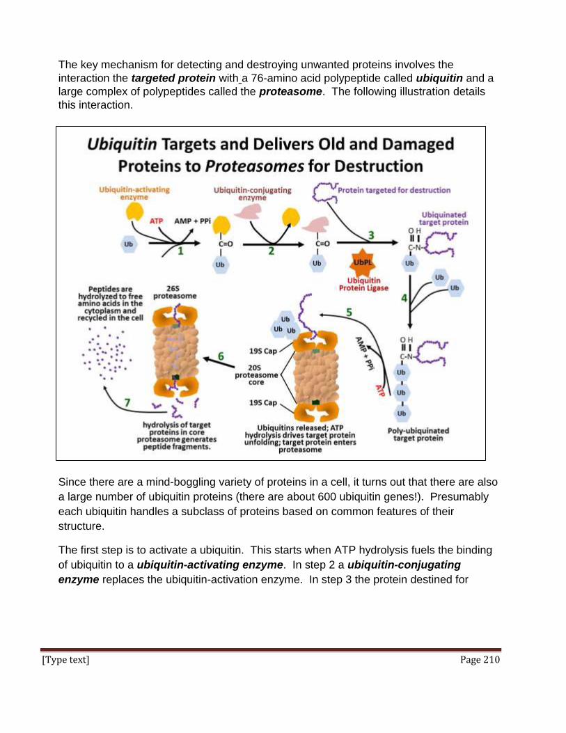
[Type text] Page 210

The key mechanism for detecting and destroying unwanted proteins involves the

interaction the targeted protein with a 76-amino acid polypeptide called ubiquitin and a

large complex of polypeptides called the proteasome. The following illustration details

this interaction.

Since there are a mind-boggling variety of proteins in a cell, it turns out that there are also

a large number of ubiquitin proteins (there are about 600 ubiquitin genes!). Presumably

each ubiquitin handles a subclass of proteins based on common features of their

structure.

The first step is to activate a ubiquitin. This starts when ATP hydrolysis fuels the binding

of ubiquitin to a ubiquitin-activating enzyme. In step 2 a ubiquitin-conjugating

enzyme replaces the ubiquitin-activation enzyme. In step 3 the protein destined for

[Type text] Page 211

destruction replaces the ubiquitin-conjugating enzyme. Several more ubiquitins bind to

this complex (step 4). Then the poly-ubiquinated protein delivers its protein to one of

the ‘CAP’ structures of the proteasome (step 5).

After binding to one of the CAP structures of a proteasome, the poly-ubiquinated target proteins dissociate. The ubiquitins are released and recycled, while the target protein unfolds (powered by ATP hydrolysis). The unfolded protein next enters the proteasome where it is digested to short peptide fragments by proteolytic enzymes in the interior of the proteasome core. The fragments are release from the CAP complex at the other end of the proteasome and digested down to free amino acids in the cytoplasm. The proteasome complex actually consists of a 20S core and two 19S CAP complexes. With its complex quaternary structure, the 26S proteasome is smaller than a eukaryotic small ribosomal subunit (40S), but is still one of the largest cytoplasmic particles… and without the benefit of any RNA in its structure! Click on this link to see an animated version of the illustration above: http://youtu.be/_g-DQq4XDfw.

Some iText & VOP Key Words and Terms

10 nm fiber galactoside transacetylase

PEP-dependent P-transferase system

3' non-transcribed DNA

gene activation phosphodiester backbone

30 nm solenoid fiber gene derepression phosphorylation cascade

5' non-transcribed DNA

gene expression pluripotent cells

adult stem cells gene induction polycistronic mRNA

allolactose gene regulation positive regulation

antisense RNA gene repression promoter

basic v. non-basic proteins

HAT enzymes proteasome

beads-on-a-string helicase protein turnover rates

-galactosidase helix-turn-helix motif proximal regulatory element

C. elegans hemin pseudogene

cAMP heterochromatin PTS

cAMP receptor protein histone acetylation regulatory genes

CAP protein histone kinases retroposon

[Type text] Page 212

CAT box histone methyl transferases

riboswitch

catabolite activator protein

histone methylation RISC

chromatin remodeling histone phosphorylation

RNA turnover rates

chromatin remodeling housekeeping genes RNA-induced silencing complex

cis-acting elements HRC kinase RNAse III (Drosha)

cistron inducer exclusion second messenger

condensed chromatin interphase O1 and O2 lac operators

developmental program

introns signal transduction

dicer lac operon siRNA (small interfering RNA)

differential gene expression

lacI gene small RNAs

distal regulatory element

lactose steroid hormone receptors

DNA bending lactose permease steroid hormones

DNAse lactose repressor structural genes

eiF2 phosphorylation lacZ, lacY and lacA genes

TATA box

EIIAGlc leucine zipper motif tetrameric lac repressor

embryonic stem cells levels of chromatin structure

totipotent cells

enhancers lncRNA transcription factors

environmental signals long non-coding RNAs transcription regulation

epigenome major groove transcription start site

euchromatin minor groove translation regulation

exons miRNA (micro RNA) trp operon

exportin negative regulation trp repressor

extended chromatin nucleosomes ubiquitin

fully differentiated cells

operator zinc finger motif

galactose operon regulation

[Type text] Page 213

Chapter 12: DNA Technologies

Manipulating DNA; cDNA libraries, Genomic Libraries, DNA Sequencing, PCR,

Microarrays, Genomics, Transcriptomics, Proteomics

I. Overview

We begin this chapter buy looking at seminal recombinant DNA technologies that led to

what we call genetic engineering. First we’ll look at cDNA (copy DNA) synthesis, a normal

process in the pathway of retrovirus reproduction. The retrovirus injects its RNA into target

cells where it transcribes a reverse transcriptase enzyme. This enzyme then reverse-

transcribes a DNA complementary to the viral RNA. Then a double stranded version of this

reverse transcript is made that replicates and directs the synthesis of new viral RNAs and

viruses. Purified versions of reverse transcriptase can be used to reverse transcribe a copy

DNA from virtually any RNA sequence. We’ll look at how a cDNA library is created and

screened for cDNA clones, and how cloned cDNAs can be used to fish out the clone of an

entire gene from a genomic library. We’ll also look at the polymerase chain reaction which

can be used to produce (amplify) millions of copies of a single gene (or other) DNA sequence

from as little DNA as is found in a single cell. Apart from its well-publicized use in forensics,

PCR remains an important laboratory tool for fetching, amplifying and studying sequences of

interest. Traditionally cloned and amplified DNA sequences have been used to study the

evolution and expression of individual genes. These venerable technologies serve here to

illustrate important principles of cloning and sequence analysis. In recent years cloning and

PCR techniques have given way to Genomics and Proteomics. These newer fields of

research leverage a growing battery of technologies to study many genes and their

regulation at the same time, allowing us to probe regulatory networks. Genomics and

Proteomics promise to get us past incomplete and even naïve notions of correlation, i.e.,

because a single genetic mutation is correlated with a genetic illness, it is the cause of the

illness. We may be soon able to identify many likely correlations that sum up to causation or

propensity to an illness.

Voice-Over PowerPoint Presentations

cDNA Libraries VOP

DNA Sequencing VOP

Genomic Libraries VOP

Polymerase Chain Reaction (PCR) VOP

Microarrays VOP.

[Type text] Page 214

Learning Objectives

When you have mastered the information in this chapter and the associated VOPs, you

should be able to:

1. Suggest molecular techniques to design experiments to test an hypothesis (specific

examples are listed below).

2. Determine when to make or use a cDNA library or a genomic library. 3. Design an experiment to purify rRNA from eukaryotic cells.

4. Design an experiment to isolate a cDNA for a human protein and clone it so you can

manufacture insulin for the treatment of disease.

5. Design an experiment using a cDNA clone or PCR product to clone a human gene.

6. Explain circumstance under which you might want to clone and express a human

growth hormone gene.

7. List the components you will need to make a cDNA library once you have isolated

poly(A) RNA from cells.

8. List the components you will need to make a genomic library once you have isolated

genomic DNA from cells.

9. Compare and contrast the use of PCR to cloning a gene from genomic DNA.

10. Choose when to use a genomic library and when to use a microarray to obtain a gene

you want to study.

11. Explain and demonstrate the logic of using fly DNA to clone or otherwise obtain copies

of a human DNA sequence.

II. Make & Screen a cDNA Library (Click to see Wikipedia’s description)

cDNAs are DNAs copied from cellular mRNAs using the enzyme reverse transcriptase.

This is the enzyme that a retroviruses like HIV uses to copy its RNA genome into DNA. It is

the copied DNA that will be made double-stranded (by the same reverse transcriptase) that

then replicates in an infected cell to make more viruses.

Under ideal conditions of cellular extraction, an mRNA isolate should represent all of the

transcripts present and being synthesized in the cell at the time of isolation. Such a

collection of mRNAs is referred to as a cell-specific transcriptome. This term is used by

analogy to genome, except that a genome is all of the genetic information of an organism,

while the transcriptome of a (typically eukaryotic) cell, is specific not only to a cell type, but to

the particular time or metabolic state of the cells at the time the mRNAs were originally

isolated! In this sense, a transcriptome reflects all of the genes being expressed in a given

cell type at a moment in time. The cDNAs that can be made and cloned from this mRNA

extract may also be referred to as a transcriptome.

[Type text] Page 215

A cDNA library is a typically a tube full of bacterial cells, each of which contains plasmids that

have been recombined with one of the many cDNAs isolated from experimental cells of

interest. When cells in this tube are spread out on an agar nutrient petri dish, each cell will

be the starting cell for a new colony of cells and each colony will contain clones of the

starting cell. cDNA libraries can be used simply to identify and determine the DNA sequence

encoding a polypeptide you are studying. Or they can be made from different cell types or

from cells of the same type but at different times or culture conditions. This allows

comparison of which genes are turned on or off in the cells.

Recall that the mature mRNA in eukaryotic cells is spliced. This means that cDNAs from

eukaryotic cells do not include introns. Introns, as well as sequences of enhancers and other

regulatory elements in and surrounding a gene must be studied in genomic libraries

(discussed below).

A. cDNA construction

mRNA is only a few percent of a eukaryotic cell; most is rRNA. But that small amount of

mRNA can be separated from other cellular RNAs by virtue of their 3’ poly(A) tails, simply

running a total RNA extract over an oligo-d(T) column (illustrated below).

The strings of Ts (thymidines) can H-bond with the poly(A) tails of mRNAs, tethering the

mRNAs on the column. All of the RNA without a 3’ poly(A) tail then flows through the

column as waste. A second buffer is passed over the column to destabilize the A-T

interactions (H-bonds) allowing elution of the mRNA fraction (below).

[Type text] Page 216

To make cDNAs from purified mRNAs, ‘free’ oligo d(T) is added to the eluted mRNA,

where it now also forms H-bonds with the poly(A) tails of the mRNAs. The oligo d(T)

serves as a primer for the synthesis of a cDNA copy of the polyadenylated mRNAs

originally in the cells. Reverse transcriptase (nowadays ‘store-bought’ but originally

isolated from chicken retrovirus-infected cells) is added next, along with DNA precursors

(the 4 deoxynucleotides), and a cDNA strand complementary to the RNA is synthesized

(below).

After heating to separate the mRNA from its cDNA, the cDNA is copied into its

complement, again using reverse transcriptase. Reverse transcriptase has the same 5’-

to-3’ DNA polymerizing activity as DNA polymerases, and so can use DNA as well as

RNA as a template. There is a short sequence at the 5’-end of most eukaryotic mRNAs

that ends up at the 3’-end of the reverse-transcribed cDNA. This sequence is

complementary to a short sequence near the 3’ end of the message, allowing formation of

a hairpin loop in which the 3’ end of the cDNA serves as a built-in primer for second-

strand synthesis (below)!

[Type text] Page 217

After the 2nd cDNA strand is made, S1 nuclease (a specifically single-stranded

endonuclease) is added to open the loop of the double stranded cDNA structure and

trimming any remaining single-stranded DNA and leaving behind a double-stranded

cDNA.

B. Cloning cDNAs into plasmid vectors

To understand cDNA cloning and other aspects of making recombinant DNA, we need to

talk about the recombinant DNA tool kit. The kit consists of several enzymes. One we

have already seen is reverse transcriptase. As noted earlier, this enzyme was originally

discovered in retrovirus-infected cells because it was required to “copy” (reverse

transcribe) retroviral RNA in infected host cells into double-stranded DNA that can be

replicated in the host cell (summarized below).

Other necessary enzymes in the ‘tool kit’ include the restriction endonucleases, or

restriction enzymes. In normal bacterial cells, these enzymes locate specific restriction

site sequences in DNA (most often palindromic DNA sequences).

[Type text] Page 218

Some restriction enzymes make the equivalent of a scissors cut through the two strands

of the double helix, leaving blunt ends. Other restriction enzymes make a staggered cut

on each strand at their restriction site, leaving behind sticky, or complementary ends

(below).

As you can imagine, two fragments of double-stranded DNA with the same sticky ends

(even in DNA from different species) can come together and form H-bonds because of

their complementary ends. That is, they can recombine! All that is left is to use DNA

ligase, another ‘tool kit’ enzyme, to form the phosphodiester linkages between the two

DNA molecules. Look for these ‘tools’ being used in the descriptions below.

1. Preparing recombinant plasmid vectors containing cDNA inserts

Vectors are carrier DNAs that are recombined with a foreign DNA of interest. When

the recombinant vector with its foreign DNA insert gets into a host cell, it can replicate

many copies of itself along with the insert DNA to be studied. Plasmids are typical

vectors for cloning cDNAs. To prepare for recombination, a plasmid vector is

digested with restriction enzyme to open the DNA circle, leaving overhanging sticky

ends. The double-stranded cDNAs to be inserted into the plasmid vectors are mixed

with linkers and DNA ligase to put a linker DNA at both ends of the ds cDNA.

[Type text] Page 219

Linkers are short double-stranded DNA oligomers containing restriction sites that can

be cut with the same restriction enzyme as the plasmid. Once the linkers have been

attached to the ends of the plasmid DNAs, they can be digested with the appropriate

restriction enzyme (usually the same one used to ‘cut’ the plasmid itself). This leaves

both the ds cDNAs and the plasmid vectors with the same (complementary) sticky

ends. These steps in the preparation of vector and ds cDNA for recombination are

illustrated below.

2. Recombining plasmids and cDNA inserts and transforming host cells

The next step is to mix the cut plasmids with the digested linker-cDNAs in just the right

proportions so that the most of the cDNA (linker) ends will anneal (form H-bonds) with

the most of the sticky plasmid ends. In early cloning experiments the goal was to

generate plasmids with only one copy of a given cDNA insert, rather than lots of re-

ligated plasmids with no inserts or lots of plasmids with multiple inserts. Using better-

engineered vector and linker combinations, this issue became less important.

[Type text] Page 220

In this example, adding DNA ligase forms the phosphodiester bonds, completing the

recombinant circle of DNA (illustrated below).

The recombinant DNA molecules are added to E. coli or other host cells that have

been made permeable so that they can be easily transformed (below).

Recall that bacterial transformation as defined by Griffith is bacterial uptake of foreign

DNA leading to a genetic change in the bacterium. The transforming principle in

this bit of genetic engineering is the recombinant plasmid! The preparation of

recombinant plasmids and their transformation into host cells is animated here:

http://youtu.be/_z-ydn718yM.

[Type text] Page 221

Not all the plasmid molecules in the mix after all these treatments are recombinant,

and some cells in the mix haven’t even taken up a plasmid. So when the recombinant

cells are plated out on agar, how does one tell which of the colonies that grow came

from cells that took up a recombinant plasmid? Both the host strain of E. coli and

plasmid vectors used these days were engineered to solve this problem. For

example, host cells chosen to be transformed are sensitive to antibiotics. On the other

hand, typical plasmid vectors were engineered to carry antibiotic resistance genes.

Recombinant cells from a library created with plasmids containing an ampicillin

resistance gene will grow on media containing ampicillin (a form of penicillin), while

cells containing non-recombinant plasmids will not grow (illustrated below).

A typical cloning plasmid will also contain a second antibiotic resistance gene, for

example streptomycin. The streptomycin resistance gene has been engineered to

contain the restriction endonuclease sites for insertion of foreign e.g., cDNAs.

So, only transformed with recombinant plasmids will grow on ampicillin agar. But

those cells may include some that were transformed by non-recombinant plasmids

(ones that do not contain an insert). The latter cells will grow on media containing

streptomycin, while cells transformed with plasmids containing an insert will NOT grow

in the presence of streptomycin. This is because the foreign DNA has been inserted

smack in the middle of the streptomycin-resistance gene, and therefore cannot

express the protein that would otherwise destroy streptomycin. We can tell apart

transformants containing recombinant plasmids from those containing non-

recombinant plasmids by the technique called replica plating.

[Type text] Page 222

After colonies grow on the ampicillin agar plate, lay a filter over the plate. The filter will

pick up a few cells from each colony, in effect becoming a replica (mirror image) of the

colonies on the plate. Place the replica filter on a new agar plate containing

streptomycin. When new colonies form, they will only be non-recombinant clones.

Finally, when you go back to the original ampicillin agar plate, you can easily identify

the recombinant colonies (below).

The replica plating procedure is animated at http://youtu.be/nemMygDhMLc.

3. Identifying colonies containing recombinant plasmids (recombinant clones)

The next step is to screen the recombinant colonies for those containing the specific

cDNA that you are after. Typically this begins with in situ lysis to break open cells

that have grown on a replica filter like the one above. In situ lysis disrupts cell walls

and membranes so that the cell contents are released and the DNA is denatured (i.e.,

becomes single-stranded). The DNA then adheres to the filter in place (in situ, where

the colonies were). The result is a filter with faint traces of the original colony (below)

In Situ Cell Lysis

[Type text] Page 223

Next, a molecular probe is used to identify DNA containing the sequence of interest.

The probe is often a synthetic oligonucleotide whose sequence was inferred from

known amino acid sequences. These oligonucleotides are made radioactive and

placed in a bag with the filter(s), where complementary sequences find each other.

The result is that colonies containing cells with recombinant plasmids containing an

insert of interest will bind the complementary probe (below).

After rinsing the filters to remove un-bound radioactive oligomers, the filters are placed

on X-ray film. After a period of exposure, the film is developed and will show a black

spot corresponding to the position of any colonies containing a recombinant plasmid

with your target sequence (below).

[Type text] Page 224

Once a positive clone is isolated, the recombinant colony is located on the original

plate, the colony is grown up in a liquid culture and the plasmid DNA is isolated.

Typically, the cloned cDNA is sequenced. The DNA sequence is then compared to

the genetic code ‘dictionary’ to verify that the cDNA insert in the plasmid in fact

encodes the protein of interest.

Cloned plasmid cDNAs can be tagged (made radioactive or fluorescent) to probe for

the genes from which they originated, locate specific mRNAs in cells, identify them in

RNA isolates from other cell types, and to quantitatively measure amounts of specific

mRNAs. Isolated plasmid cDNAs can even be expressed in suitable cells to make the

encoded protein. The synthetic insulin given to diabetics these days is no longer pig

insulin, but is made from expressed human cDNAs. While the introduction of the

polymerase chain reaction (PCR, see below) has superseded some uses of cDNAs,

they still play a role in genome-level studies of e.g., the transcriptome.

III. DNA sequencing (Click to see Wikipedia’s description)

A. A Brief History of DNA Sequencing

RNA sequencing came first, when Robert Holley sequenced a tRNA in 1965. tRNA

sequencing was possible because the bases in tRNAs were chemically modified after

transcription, and because tRNAs are short! Many tRNAs were eventually sequenced

directly. An early method for sequencing DNA involving DNA fragmentation was

developed by Walter Gilbert and colleagues. Frederick Sanger in England developed a

DNA synthesis-based ‘dideoxy’ method of sequencing that quickly became the DNA

sequencing standard. Sanger and Gilbert won a Nobel Prize in 1983 for their DNA

sequencing efforts.

The first complete genome to be sequenced was that of a bacteriophage (bacterial virus)

called φX174. At the same time as the advances in sequencing technology were

occurring, so were some of the early developments in recombinant DNA technology.

Together these led to the sequencing of DNA from more diverse sources than viruses.

The first focus was on sequencing the genes and genomes of important model

organisms, such as E. coli, C. elegans and yeast (S. cerevisiae). By 1995, Craig Venter

and colleagues at the Institute for Genomic Research had completed the sequence of an

entire bacterial genome (Haemophilus influenzae) and by 2001, Venter’s private group

along with Frances Collins and colleagues at the NIH had published a first draft of the

sequence of the human genome. Venter had proved the efficacy of a whole-genome

sequencing approach called shotgun sequencing, which was much faster than the gene-

by-gene, fragment-by-fragment ‘linear’ sequencing strategy being used by other

investigators (more later!).

[Type text] Page 225

B. Details of DiDeoxy Sequencing

Sanger’s sequencing method is based on two key technologies:

1. The ability to replicate template different length fragments of DNA from a template

DNA whose sequence you want to determine.

2. The ability to identify the last nucleotide on each newly made DNA fragment.

Since the Sanger dideoxynucleotide DNA sequencing method remains the most common

and economical, let’s consider the basics of the protocol.

Deoxynucleotides contain a ribose missing its 2’ OH (hydroxyl) group. Phosphodiester

bonds formed during replication link the phosphate of a free nucleotide triphosphate

to the 3’ OH of a deoxynucleotide at the end of a growing DNA strand.

Dideoxynucleotide triphosphates are missing the 2’ AND 3’ OH groups on the sugar

(shown as the hydrogen in red below).

As a result, if this nucleotide is added to the end of a growing DNA strand, no further

nucleotides can be added (the 3’–OH is necessary for the dehydration synthesis of the

next phosphodiester bond). A look at the original form of manual sequencing

reveals what is going on in the sequencing reaction.

[Type text] Page 226

Four reaction tubes are set up, each containing the template DNA to be sequenced, a

primer and the 4 deoxynucleotide precursors necessary to replicate DNA (illustrated

below).

Each tube also contains a different dideoxynucleotide (ddATP, ddCTP, ddGTP or ddTTP).

To start the sequencing reaction, DNA polymerase is added to each tube. to start the

DNA synthesis reaction. During DNA synthesis, different length fragments of new DNA

are generated as the ddNTPs are incorporated at random opposite complementary bases

in the template DNA being sequenced (below).

A short time after adding the DNA polymerase to begin the reactions, the mixture is

heated to separate the DNA strands and fresh DNA polymerase is added to repeat the

synthesis reactions. These sequencing reactions are repeated as many as 30 times in

order to produce enough radioactive DNA fragments to be detected. With the advent

of Taq polymerase from the thermophilic bacterium Thermus aquaticus, it became

unnecessary to add fresh DNA polymerase after each replication cycle. The mixture

could be heated and cooled at will without destroying the Taq DNA polymerase. Finally,

the many cycles of chain-termination sequencing were automated by using

programmable thermocyclers.

[Type text] Page 227

Since a small amount of a radioactive deoxynucleotide (usually 32P-labeled ATP) was

present in each reaction tube, the newly made DNA fragments were radioactive. The

new DNA fragments from each tube are separated by electrophoreses. An

autoradiograph of the gel then reveals the position of each terminated fragment, from

which the DNA sequence can be read. A simulated gel is shown below.

The first semi-automated DNA sequencing method was invented in Leroy Hood’s

California lab in 1986. This was still Sanger sequencing, but in this method, the 4

dideoxynucleotides in the sequencing reaction were tagged with a fluorescent dye.

Instead of requiring radioactive phosphate-tagged nucleotides for DNA fragment

detection, each dye-terminated DNA strand could be detected by its fluorescence. The

color of fluorescence indicated which base terminated the DNA chain as it passed

through a fluorescence detector, the smallest chains first, followed by the longer ones. A

computer generated color-coded graph like the one below shows the order (and therefore

length) of the fragments passing the detector and thus, the sequence of the strand.

[Type text] Page 228

Hood’s innovations were quickly commercialized making major sequencing projects

possible, including whole genome sequencing. The rapidity of automated DNA

sequencing led to the creation of large sequence storage databases in the U.S. and

Europe. The U.S. database is maintained at the NCBI (National Center for Biological

Information). Despite its location, the NCBI archives virtually all DNA sequences

determined worldwide. With newer sequencing methods (some are described below) the

databases and the tools to find, compare and otherwise analyze DNA sequences have

grown by leaps and bounds.

C. Large scale sequencing

Large scale sequencing targets entire prokaryotic genomes and eukaryotic chromosomes

(typically much larger than any bacterial genome) and requires strategies that either

sequence long DNA fragments and/or sequencing DNA fragments more quickly. We

already noted shotgun sequencing, used by Venter to sequence smaller and larger

genomes (including our own… or more accurately, his own!). Shotgun sequencing is

summarized below.

[Type text] Page 229

In shotgun sequencing, long cloned DNA fragments as long as or longer than 1000 base

pairs are broken down at random into smaller, more easily sequenced fragments. The

fragments are themselves cloned and sequenced, and non-redundant sequences are

assembled by aligning overlapping regions of sequence. Computer software these days

are quite adept at rapidly aligning short overlapping sequences and displaying long

contiguous DNA sequences.

Sequence gaps that remain after shotgun sequencing can be filled in by primer walking,

in which a known sequence near the gap is the basis of creating a sequencing primer to

“walk” into the gap region on an intact DNA that has not been fragmented. Another

technique involves PCR (the Polymerase Chain Reaction, described later), in which two

oligonucleotides are synthesized based on sequence information on either side of a gap,

and used to synthesize the missing fragment, which can then be sequenced to foil in the

gap.

IV. Genomic Libraries (Click to see Wikipedia’s description)

A. Overview

A genomic library might be a tube full of recombinant bacteriophage. Each phage

DNA molecule contains an insert, a fragment of cellular DNA from a foreign organism.

The library is made so that it contains a representation of all of possible fragments of that

genome. The viral genomes of bacteria were used clone genomic DNA fragments

because:

they could be engineered to remove a large amount of DNA that is not needed

infection and replication in bacterial host cells.

the missing DNA could be replaced by fragments of foreign insert DNA as long as 18-

20kbp (kilobase pairs), nearly 20 times as long as typical cDNA inserts.

purified phage coat proteins could be mixed with the recombined phage DNA to make

infectious phage particles that would infect host bacteria, replicate lots of new

recombinant phage, and then lyse the cells to release the phage.

The need for vectors like bacteriophage that can accommodate long inserts becomes

obvious from the following bit of math. A typical mammalian genome consists of more

than 2 billion base pairs. Inserts in plasmids are very short, rarely exceeding 1000 base

pairs. Dividing 2,000,000,000 by 1000, you get 2 million, a minimum number of phage

clones that would need to be screened to find a sequence of interest. In fact, you would

need many more than this number of clones to find a gene. Part of the solution to this

“needle in a haystack” dilemma was to clone larger DNA inserts in suitable vectors.

[Type text] Page 230

From this brief description, you may recognize the common strategy for genetically

engineering a cloning vector: Determine the minimum properties that your vector must

have and remove non-essential DNA sequences. Consider the Yeast Artificial

Chromosome (YAC), hosted by (replicated in) yeast cells. YACs can accept humongous

foreign DNA inserts! This is because to be a eukaryotic chromosome requires one

centromere and two telomeres… and little else! Recall that telomeres are needed in

replication to keep the chromosome from shortening during replication of the DNA. The

centromere is needed to attach chromatids to spindle fibers so that they can separate

during anaphase in mitosis (and meiosis). So along with a centromere and two

telomeres, just include restriction sites to enable recombination with inserts as long as

2000 Kbp. That’s a YAC! Getting the YAC is the easy part. Keeping a 2000Kbp long

DNA fragment intact long enough to get it into the YAC is the challenge.

Whatever the vector chosen and however they are obtained, sequences of genomic DNA

can show us how a gene is regulated by revealing known and uncovering new regulatory

DNA sequences. They can tell us what other genes are nearby, and where genes are on

chromosomes. They can be used to find similar sequences in different species and

comparative sequence analysis can tell us a great deal about gene evolution and the

evolution of species. One early surprise from gene sequencing studies was that we share

many common genes and DNA sequences with other species, from yeast to worms to

flies… and of course mammals and other vertebrates. You probably know that our

human genome and the chimpanzee genome are 99% similar. And we have already

seen comparative sequence analysis that showed how proteins with different functions

nevertheless share structural domains.

B. Preparing Recombinant Genomic Clones

1. Preparing Genomic DNA of a Specific Length for Cloning

Let’s look at the approach to cloning a genomic library in phage – the principles would

apply to any genomic cloning operation, but the numbers and details used here

exemplify cloning in phage. To begin with, high molecular weight (i.e., long molecules

of) the desired genomic DNA are isolated and purified and then digested with a

restriction enzyme. Usually, the digest is partial, aiming to generate overlapping

fragments of random length DNA. When the digest is electrophoresed on agarose

gels, the DNA (stained with ethidium bromide, a fluorescent dye that binds to DNA)

looks like a bright smear on the gel (e.g., below). All of the DNA could be recombined

with suitably digested vector DNA. But to further reduce the number of clones to be

screened for a sequence of interest, early cloners would generate a Southern blot to

determine the size of genomic DNA fragments most likely to contain a desired gene.

[Type text] Page 231

Briefly here is the protocol for making a Southern blot (named after Edward Southern,

the inventor of the technique) and cloning inserts of a specific size:

a) Digest genomic DNA with one or more restriction endonucleases.

b) Run the digest products on an agarose gel to separate the fragments by size

(length). The DNA will appear as a smear when stained with a fluorescent dye.

c) Place a filter on the gel. Over several hours, the DNA will be blotted to the filter.

d) Remove the filter and place it in a bag in a solution that can denature the DNA.

e) Add a radioactive probe (e.g., cDNA) containing the gene or sequence of interest.

The probe will hybridize (bind) to a complementary genomic sequence on the filter.

f) Prepare an autoradiograph of the filter and see a ‘band’ representing the size of

genomic fragments of DNA that include the sequence of interest.

g) Run another gel of the digested genomic DNA and using the information from the

Southern blot, cut out the piece of gel containing the fragments that ‘lit up’ in the

autoradiograph.

h) Remove the DNA from the gel piece and use it as the source of inserts for genomic

cloning.

These steps are illustrated below.

[Type text] Page 232

2. Recombining Size-Restricted Genomic DNA with Phage DNA

The Southern blot allows identification of a set of restriction enzymes that generates

18-20 Kbp genomic DNA fragments that hybridize to the probe. More genomic DNA is

digested with the same set of restriction enzymes and then separated on an agarose

gel. A chunk of agarose containing only those fragments ranging between 18kbp and

20kbp is excised from the gel. The DNA in this gel chunk is isolated and mixed with

compatibly digested phage DNA at concentrations that favor the formation of H-bonds

between the ends of the phage DNA and the genomic fragments. The addition of

DNA ligase covalently links the recombined DNA molecules. These steps are

abbreviated in the illustration below.

[Type text] Page 233

3. Creating Infectious Viral Particles with Recombinant phage DNA As noted, the recombined phage DNA can be introduced into a bacterial host by adding viral coat proteins to make infections phage (below).

The phage are added to a tube-full of host bacteria. Infection follows and the

recombinant DNA enters the cells where it replicates and directs the production of new

phage that eventually lyse the host cell (illustrated below).

[Type text] Page 234

The recombined vector can also be introduced directly into the host cells by

transduction (which is to phage DNA what transformation is to plasmid DNA).

Whether by infection or transduction, the recombinant phage DNA ends up in host

cells which produce new phage that lyse the host cell. The released phages go on to

infect more host cells until all cells have lysed. What remains is a tube full of lysate

containing cell debris and recombinant phage particles.

4. A Note About Some Other Vectors

As we see comparing plasmids to phage DNA vectors, different vectors can

accommodate different size inserts. For larger genomes, the need is to choose a

vector able to house larger insets so that you end up screening the minimum number

of clones. Given a large enough eukaryotic genome, it may be necessary to screen

more than a hundred thousand clones in a phage –based genomic library. Apart from

size-selection of genomic fragments before inserting them into a vector, selecting the

appropriate vector is just as important. The table below lists commonly used vectors

and the sizes of inserts they will accept.

Vector type Insert size (thousands

of bases)

Plasmids up to 15

Phage lambda (λ) up to 25

Cosmids up to 45

Bacteriophage P1 70 to 100

P1 artificial chromosomes (PACs) 130 to 150

Bacterial artificial chromosomes (BACs) 120 to 300

Yeast artificial chromosomes (YACs) 250 to 2000

Click on the vectors to learn more about them. We’ll continue this example by looking at how recombinant phage in a genomic library are screened for a genomic sequence of interest.

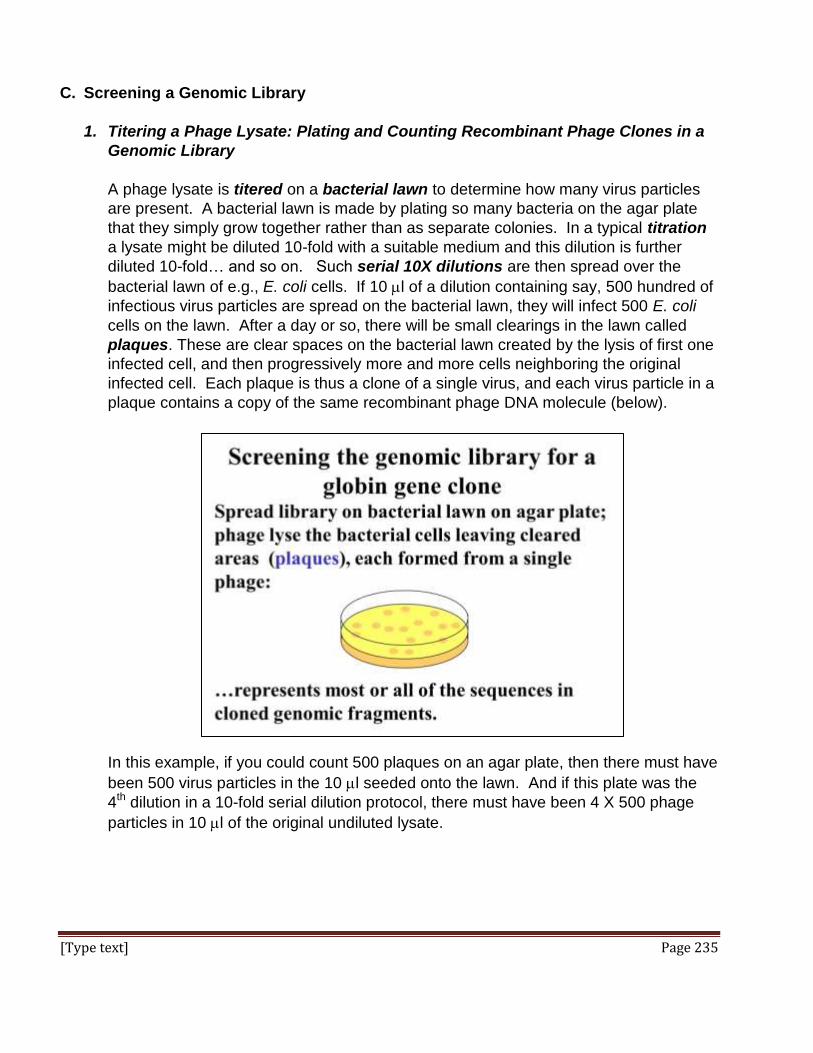
[Type text] Page 235

C. Screening a Genomic Library

1. Titering a Phage Lysate: Plating and Counting Recombinant Phage Clones in a

Genomic Library

A phage lysate is titered on a bacterial lawn to determine how many virus particles

are present. A bacterial lawn is made by plating so many bacteria on the agar plate

that they simply grow together rather than as separate colonies. In a typical titration

a lysate might be diluted 10-fold with a suitable medium and this dilution is further

diluted 10-fold… and so on. Such serial 10X dilutions are then spread over the

bacterial lawn of e.g., E. coli cells. If 10 l of a dilution containing say, 500 hundred of

infectious virus particles are spread on the bacterial lawn, they will infect 500 E. coli

cells on the lawn. After a day or so, there will be small clearings in the lawn called

plaques. These are clear spaces on the bacterial lawn created by the lysis of first one

infected cell, and then progressively more and more cells neighboring the original

infected cell. Each plaque is thus a clone of a single virus, and each virus particle in a

plaque contains a copy of the same recombinant phage DNA molecule (below).

In this example, if you could count 500 plaques on an agar plate, then there must have

been 500 virus particles in the 10 l seeded onto the lawn. And if this plate was the

4th dilution in a 10-fold serial dilution protocol, there must have been 4 X 500 phage

particles in 10 l of the original undiluted lysate.

[Type text] Page 236

2. Probing the Genomic Library

In order to represent a complete genomic library, it is likely that many plates of such a

dilution (~500 plaques per plate) will have to be created and then screened for a

plaque containing a gene of interest. If only size-selected fragments were inserted

into the phage vectors, the plaques will represent a partial genomic library, requiring

screening fewer clones to find the sequence of interest. For either kind of library, the

next step is to make replica filters of the plaques. Replica plating of plaques is similar

to making a replica filter bacterial colonies. But in this case, there will be DNA in the

plaque replicas that never got packaged into viral particles. The filters can be treated

to denature this DNA and can then be probed directly with a known sequence

In the early days of cloning, this probe was usually an already isolated and sequenced

cDNA clone, either from the same species as the genomic library, or from a cDNA

library of a related species. After soaking the filters in a tagged (radioactive) probe, X-

Ray film is placed over the filter, exposed and developed. Black spots will form where

the film lay over a plaque containing genomic DNA complementary to (and therefore

hybridized to) the radioactive probe, as illustrated below.

3. Isolating a Gene for Further Study

Genomic clones are typically much larger (longer) than any gene of interest, and

always longer than any cDNA from a cDNA library. They are also embedded in a

genome that is thousands of times as long as the gene itself. As noted earlier,

[Type text] Page 237

cloning large chunks of a genome in commodious vectors reduces the number of

clones to be screened for a gene. If the genome can be screened among a

reasonable number of cloned phage (under 100,000 plaques for instance)., the one

plaque containing a positive signal would be further studied. To find out where a gene

is in a large genomic clone (20+kbp long), the traditional strategy is to purify the

cloned DNA, digest it with restriction endonucleases and separate the digest particles

by agarose gel electrophoresis. Using Southern Blotting, the separated DNA

fragments are denatured and blotted to a nylon filter. The filter is then probed with the

same tagged probe used to find the positive clone (plaque). The smallest DNA

fragment containing the gene of interest will usually be the object of further study and

analysis. Such fragments can themselves be subcloned (in suitable vectors) and

grown to provide enough DNA to further study the gene.

V. The Polymerase Chain Reaction (PCR) (Click to see Wikipedia’s description)

The polymerase chain reaction (PCR) can amplify a region of DNA from any source, even

from a single cell’s worth of DNA or from fragments of DNA obtained from a fossil. This

amplification, which can take just a few hours, can generate millions of copies of the desired

target DNA sequence, in effect purifying the DNA from surrounding sequences in a single

reaction!. Kary B. Mullis was awarded a Nobel prize in 1993 for his development of PCR,

which is now the basis of innumerable molecular strategies for producing DNAs for research

in gene structure, function and evolution as well as in criminal forensics, medical diagnostics

and other commercial uses. PCR is described in detail below.

A. PCR – the Basic Process

PCR relies on using some bits of known DNA sequence, such as that of a cDNA, to

design short oligonucleotide sequences (oligomers) that are then synthesized in the

laboratory. The oligomers are chosen to be complementary to sequences near the

opposite ends of the known DNA sequence such that the oppose (face) each other. That

just means that the 3’ end of one oligomer faces the 3’ end of the opposing oligomer.

This way the two oligomers can serve as primers for the elongation replication of both

strands of a double stranded target DNA sequence. The primers are added to the target

DNA source from which a gene is to be amplified by PCR.

The mixture is then heated to denature the target DNA. After cooling the mixture to allow

the primers to H-bond with their complementary target DNA strands, the four

deoxynucleotide precursors to DNA (dATP, dCTP, dTTP and dGTP) are added along with

a small amount of a DNA polymerase. This allows elongation of new DNA strands from

the oligonucleotide primers on the template DNAs.

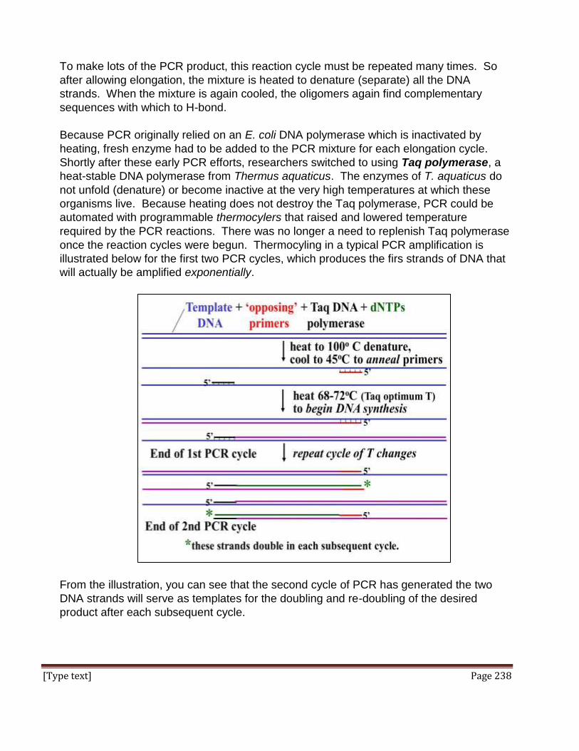
[Type text] Page 238

To make lots of the PCR product, this reaction cycle must be repeated many times. So

after allowing elongation, the mixture is heated to denature (separate) all the DNA

strands. When the mixture is again cooled, the oligomers again find complementary

sequences with which to H-bond.

Because PCR originally relied on an E. coli DNA polymerase which is inactivated by

heating, fresh enzyme had to be added to the PCR mixture for each elongation cycle.

Shortly after these early PCR efforts, researchers switched to using Taq polymerase, a

heat-stable DNA polymerase from Thermus aquaticus. The enzymes of T. aquaticus do

not unfold (denature) or become inactive at the very high temperatures at which these

organisms live. Because heating does not destroy the Taq polymerase, PCR could be

automated with programmable thermocylers that raised and lowered temperature

required by the PCR reactions. There was no longer a need to replenish Taq polymerase

once the reaction cycles were begun. Thermocyling in a typical PCR amplification is

illustrated below for the first two PCR cycles, which produces the firs strands of DNA that

will actually be amplified exponentially.

From the illustration, you can see that the second cycle of PCR has generated the two

DNA strands will serve as templates for the doubling and re-doubling of the desired

product after each subsequent cycle.

[Type text] Page 239

A typical PCR reaction might involve 30 PCR cycles, resulting in a nearly exponential

amplification of the desired sequence.

The amplified products of PCR amplification products are in such abundance that they

can easily be seen under fluorescent illumination on an ethidium bromide-stained agarose

gel (below).

In this gel, the first lane contains a DNA ladder, which is a mixture of DNAs of known

lengths that can be used to size the PCR fragments in the adjacent lanes. The gel lane

next to the ladder is empty, while the two bright bands in the 3rd and 4th lanes are PCR

products generated with two different oligomer primer pairs. PCR-amplified DNAs can be

sequenced and then used in many subsequent studies.

B. The many Uses of PCR

PCR-amplified products can be labeled with radioactive or fluorescent tags to serve as

hybridization probes for clone isolation from cDNA or genomic libraries, or on Southern

blots (or northern blots, a more fanciful name for RNAs that are separated by size on gels

and blotted to filters). We noted above that PCR has wide applications to research,

medicine and other practical applications. A major advance was Quantitative PCR,

applied to studies of differential gene expression and gene regulation. In Quantitative

PCR, initial cDNAs are amplified to detect not only the presence, but the relative amounts

of specific transcripts being made in cells.

Adapted from: http://upload.wikimedia.org/wikipedia/commons/e/e6/AgarosegelUV.jpg

[Type text] Page 240

Another application of PCR is in the forensics, to identify a person or organism by

comparing its DNA to some standard, or control DNA. An example of a gel showing

these DNA fingerprints is shown below.

The ability of PCR fingerprinting to detect genetic relationships between near and distant

relatives (and to exclude such relationships), is the basis of solving crimes and the

discrimination of paternity, as well as evolutionary relationships between organisms. A

video on DNA fingerprinting is at the following link: Alu and DNA fingerprinting. Alu is a

highly repeated ~300bp DNA sequence found throughout the human genome. Alu

sequences are short interspersed elements, or SINES, a category of mobile, or

transposable elements (transposons). DNA fingerprinting is

possible in part because each of us has a unique number and distribution of Alu SINEs in

our genome. You can read more about Alu sequences and human diversity at

http://www.ceinge.unina.it/~zollo/Studenti/alu.pdf.

From: http://www.dnalc.org/view/15582-DNA-fingerprint.html

[Type text] Page 241

Intriguing examples of the use of PCR for identification include establishing the identities

of Egyptian mummies, the Russian Tsar deposed during the Russian revolution, and the

recently unearthed body of King Richard the 3rd of England. Variant PCR protocols and

applications are manifold and often quite inventive! A list is presented at this link:

Variations on Basic PCR.

VI. Genomic Approaches: The DNA Microarray (Click to see Wikipedia’s

description)

Where cell levels of a protein are known to change in response to a chemical effector,

molecular studies traditionally focused on control of transcription of its gene. These studies

often revealed that the control of gene expression was at the level of transcription, turning a

gene on or off through interactions of transcription factors with DNA. However, control of a

protein level sometimes turns out to be post-transcriptional, at the level of the rate of mRNA

degradation or of translation. Such studies were seminal to our understanding of how a gene

is controlled and how the right correct protein is made at the right time.

We might have suspected, but now we know that control of gene expression and cellular

responses can be more complex than increasing the transcription of a single gene or

translation of a single protein. Whole genome sequences and new techniques make

possible the study of the expression of virtually all genes in a cell at the same time, a field of

investigation called genomics. Genomic studies reveal a web, or network of responses that

must be understood to more fully explain developmental and physiological changes in an

organism. When you can ‘see’ all of the genes that are active in a cell or tissue, you are

looking at its transcriptome, an area of study sometimes called transcriptomics. The study

of which proteins are being synthesized in a cell or a tissue, how they are modified

(processed) before use and how much of each is being synthesized is called proteomics.

The technologies applied to proteomic studies include proteins microarrays immunochemical

techniques and other uniquely suited to proteins analysis (see

http://en.wikipedia.org/wiki/Proteomics for more).

Microarray technology involves ‘spotting’ cloned DNA (oligonucleotides, PCR products, or

DNA from a genomic or cDNA library) on a glass slide, or chip. In the language of microarray

analysis, the slides are the probes. Spotting a chip is a robotic process, animated in this

link: http://youtu.be/p2zxwQl8n9s. Because the DNA spots are microscopic,

oligonucleotides, PCR products, or a cell-specific transcriptome (cDNA library) can usually be

accommodated on a single chip. A small genome microarray might also fit on a single chip,

while larger genomes might need several slides.

[Type text] Page 242

A primary use of DNA microarrays is transcriptional profiling. A genomic microarray can

probe a mixture of fluorescently tagged target cDNAs made from mRNAs, in order to identify

which genes are expressed in the cells, or its transcriptome. A cDNA microarray can probe

quantitative differences in gene expression in cells or tissues during normal differentiation or

in response to chemical signals. They are also valuable for genotyping, (i.e. characterizing

the genes in an organism).

Microarrays are so sensitive that they can even distinguish between two genes or regions of

DNA that differ by a single nucleotide. Such differences are called SNPs, or single

nucleotide polymorphisms (click the link to learn more). After probing with one or more

fluorescence-tagged nucleic acids, the microarray is viewed in a fluorescent microscope

(below).

The UV light in the microscope causes spots to fluoresce a different color for each

fluorescently tagged target molecule that has hybridized to probe sequences on the

microarray. When quantitative microarray procedures are used, the brightness of the signal

from each probe can be measured and is an indication of the amount of nucleic acid bound

to the spot on the array, or the relative amounts of cDNA (and therefore RNA) from different

tissues or tissue treatments hybridizing to the same spot on identical microarrays. On the

next page is a table of different applications of microarrays (adapted from Wikipedia).

From: A Microarray

Microarray on a glass slide

[Type text] Page 243

Application or technology Synopsis

Gene expression profiling

In a transcription( mRNA or gene expression) profiling

experiment the expression levels of thousands of genes are

simultaneously monitored to study the effects of certain

treatments, diseases, and developmental stages on gene

expression.

Comparative genomic hybridization

Assessing genome content in different cells or closely related

organisms, where one organism’s genome is the probe for a

target genome from a different species.

GeneID

Small microarrays to check IDs of organisms in food and feed for

genetically modified organisms (GMOs), mycoplasms in cell

culture, or pathogens for disease detection. These detection

protocols often combine PCR and microarray technology.

Chromatin immunoprecipitation on Chip

(ChIP)

DNA sequences bound to a particular protein can be isolated by

immunoprecipitating that protein. These fragments can be then

hybridized to a microarray (such as a tiling array) allowing the

determination of protein binding site occupancy throughout the

genome.

DamID

Analogously to ChIP, genomic regions bound by a protein of

interest can be isolated and used to probe a microarray to

determine binding site occupancy. Unlike ChIP, DamID does not

require antibodies but makes use of adenine methylation near the

protein's binding sites to selectively amplify those regions,

introduced by expressing minute amounts of protein of interest

fused to bacterial DNA adenine methyltransferase.

SNP detection

Identifying single nucleotide polymorphism among alleles within

or between populations. Several applications of microarrays

make use of SNP detection, including Genotyping, forensic

analysis, measuring predisposition to disease, identifying drug-

candidates, evaluating germline mutations in individuals or

somatic mutations in cancers, assessing loss of heterozygosity, or

genetic linkage analysis.

Alternative splicing detection

An exon junction array design uses probes specific to the

expected or potential splice sites of predicted exons for a gene. It

is of intermediate density, or coverage, to a typical gene

expression array (with 1-3 probes per gene) and a genomic tiling

array (with hundreds or thousands of probes per gene). It is used

to assay the expression of alternative splice forms of a gene.

Exon arrays have a different design, employing probes designed

to detect each individual exon for known or predicted genes, and

can be used for detecting different splicing isoforms.

Tiling array

Genome tiling arrays consist of overlapping probes designed to

densely represent a genomic region of interest, sometimes as

large as an entire human chromosome. The purpose is to

empirically detect expression of transcripts or alternatively

spliced forms which may not have been previously known or

predicted.

[Type text] Page 244

Some iText & VOP Key Words and Terms

2', 3' di-deoxy CTP chemotherapy genome regulatory networks

alternative splicing genome projects restriction endonucleases

automated DNA sequencing genomic library reticulocyte

autoradiography insert DNA reverse transcriptase

BACs and YACs library screening RNA probes

bacterial artificial chromosome vectors linkers RNAse

blunt ends Northern blot shotgun sequencing

cDNA oligo d(T) column single nucleotide polymorphisms

cDNA hairpin loop PCR SNPs

cDNA library PCR Southern blot

cDNA probes PCR primers sticky ends

chemiluminescence PCR steps systematics

cosmid vectors phage lambda vectors Taq polymerase

di-deoxy chain termination plasmids thermophilic bacteria

di-deoxy sequencing method poly(A) tail thermophilic DNA polymerases

DNA ligase polymerase chain reaction Thermus aquaticus

DNA sequencing primer transcriptome

elution primer walking transformation

ethidium bromide probe hybridization vectors

fluorescence proteome Western blot

forensics recombinant vector yeast artificial chromosome vectors

Genetic (DNA) fingerprint recombination

[Type text] Page 245

Chapter 13: Membrane Structure

Membrane Structure and Function: the fluid mosaic, membrane proteins,

glycoproteins, glycolipids

I. Overview

All intracellular membranes, including the plasma membrane, share a common

phospholipid bilayer construction. All membranes are a fluid mosaic of proteins attached

to or embedded in the phospholipid bilayer. The different proteins in cellular membranes are

key in making one kind of membrane structurally and functionally different from another.

Integral membrane (Transmembrane) proteins span the lipid bilayer. They are

characterized by a hydrophobic domain and two hydrophilic domains. In the case of the

plasma membrane, the hydrophilic domains interact with the aqueous extracellular fluid on

one side and the cytoplasm on the other, while a hydrophobic domain keeps the proteins

attached to the membrane. Once embedded in the fatty acid interior of a membrane, integral

membrane proteins cannot escape! Peripheral membrane proteins bind to membrane

surfaces, typically held in place by hydrophilic interactions between the protein and charged

features of the membrane surface (phospholipid heads, hydrophilic surface domains of

integral proteins). Recall that extracellular surfaces are “sugar coated” because the integral

proteins are often glycoproteins that expose their sugars to the outside of the cell. Thus cells

present a glycocalyx to the outside world. As cells form tissues and organs, they become

bound to extracellular proteins and glycoproteins that they themselves or other cells secrete,

to form an extracellular matrix. Using mainly the plasma membrane, we’ll look at

characteristic structures and biological activities of membrane proteins that inform their

specific functions.

Voice-Over PowerPoint Presentations

Membrane Structure VOP

Structure of Membrane Proteins VOP

Learning Objectives

When you have mastered the information in this chapter and the associated VOPs, you

should be able to:

1. distinguish components of the membrane that can move (diffuse) laterally in the

membrane from those that can flip (switch from the outer to the inner surface of the

phospholipid bilayer).

2. compare the fluid mosaic membrane to earlier membrane models and cite the evidence for and against each (as appropriate).

[Type text] Page 246

3. describe how the plasma membrane is made by the cell, and suggest an experiment

that would demonstrate your hypothesis.

4. distinguish between transmembrane and peripheral membrane proteins, provide

specific examples of each.

5. decide whether or not a newly discovered protein might be a membrane protein.

6. predict the effect of molecular and physical influences on membrane fluidity.

7. suggest how organisms living in warm tropical waters have adapted to the higher

temperatures. Likewise, fish living under the arctic ice.

8. explain how salmon are able to spend part of their lives in the ocean and part swimming

upstream in freshwater to spawn without their cells shriveling of exploding!

9. list the diverse functions of membrane proteins.

10. speculate on why only eukaryotic cells have evolved to have sugar-coated cell surfaces.

11. compare and contrast the glycocalyx and extracellular matrix of some cells.

II. Plasma Membrane Structure (Click to see Boundless.com’s description) The cell or plasma membrane surrounds the cytoplasm within cells, which in eukaryotes is

filled with membrane-bound organelles. All cellular membranes are selectively permeable

(semi-permeable), allowing only certain substances to cross the membrane. All cellular

membranes are composed of two layers of phospholipids embedded with proteins and

glycoproteins. Different phospholipid and protein compositions give different cellular

membranes their unique functions. Decades of research have reveled these functions (see

earlier discussions of mitochondrial and chloroplast function for instance). Here we will

describe general features of membranes, using the plasma membrane as our example.

A. The Phospholipid Bilayer

A bilayer membrane structure was predicted by Gorter and Grendel as early as 1925.

They knew that red blood cells (erythrocytes) have no nucleus or other organelles, and

thus have only a plasma membrane. They also knew that a major chemical component of

these membranes were lipids, specifically phospholipids. Basic phospholipid structure

as we understand it today is shown in the space-filling molecular model below,

highlighting its hydrophilic (polar) head and hydrophobic tails. Molecules with

hydrophilic and hydrophobic domains are called amphipathic.

[Type text] Page 247

By the early 1900s, Gorter and Grendel had experimentally measured the surface area of

red blood cells, disrupted them and calculated the amount of phospholipids in the

membranes that remained. Although Gorter and Grendel made two calculation errors,

their mistakes compensated each other. So their estimate that there were enough lipid

molecules per cell to wrap around each cell twice was prophetic if not strictly speaking,

‘correct’!

Common membrane phospholipids are shown below.

When amphipathic molecules are mixed with water they will spontaneously aggregate to

‘hide’ their hydrophobic regions from the water. Phospholipids in water will aggregate so

that polar heads face away from each other and the hydrophobic tails interact with each

other. Knowledge that membranes were composed of phospholipids led to a picture of

membrane architecture based on phospholipid interactions (below).

[Type text] Page 248

B. Models of Membrane Structure

In 1935, Davson and Danielli suggested that proteins might be more or less fortuitously

bound to the polar heads of the phospholipids. J.D. Robertson first observed membranes

in the transmission electron microscope at high power some decades later, revealing

them to have a trilamellar structure (below).

The trilamellar structure was consistent with the biochemical evidence of a phospholipid

bilayer in which the clear layer was interpreted as the lipid region of the membrane. The

electron-dense regions facing the aqueous regions inside and outside the cell would be

the polar heads of the phospholipids, associated with the polar surfaces of proteins. This

seemed to confirm the Davson-Danielli model, though Robertson offered his Unit

Membrane theory in which only proteins with specific functions associated with a

membrane were actually bound to the phospholipid heads.

The static view of the trilamellar models of membrane structure implied by the Davson-

Danielli or Robertson models were replaced in 1972 when Singer and Nicolson proposed

the Fluid Mosaic model of membrane structure. They suggested that in addition to

peripheral proteins that do bind to the surfaces of membranes, many integral

membrane proteins actually span the membrane. Integral membrane proteins were

imagined as a mosaic of protein ‘tiles’ embedded in a phospholipid medium. But unlike a

mosaic of glazed tiles set in a firm, cement-like structure, the protein ‘tiles’ were predicted

to be mobile (fluid) in a phospholipid sea. The key to the fluid mosaic is that embedded

proteins are held in membranes by a hydrophobic domain, while they expose their

hydrophilic domains to the external aqueous and cytosolic environments. Because the

hydrophilic domains of each integral membrane protein are different from each other, we

say that cellular membranes are asymmetric. In other words, cells expose different

surface structural (and functional) features to opposite sides of the membranes.

[Type text] Page 249

A typical model of the plasma membrane of a cell is illustrated below (peripheral proteins

are designated as a “Surface protein”).

Because of their own aqueous hydrophilic domains, membrane proteins are a natural

barrier to the free passage of charged molecules across the membrane. On the other

hand, membrane proteins are responsible for the selective permeability of membranes,

facilitating the movement of specific molecule in and out of cells. Membrane proteins also

account for specific and selective interactions with their extracellular environment,

including the adhesion of cells to other cells, their attachment to surfaces, communication

between cells (both direct and via hormones and neurons), etc.. The extracellular surface

of plasma membranes is ‘sugar-coated’ with oligosaccharides covalently linked to

membrane proteins (as glycoproteins) or to phospholipids (as glycolipids). The

carbohydrate components of glycosylated membrane proteins inform their function. For

example, the glycoproteins enable specific interaction of cells with each other to form

tissues. They also allow interaction with extracellular surfaces to which they must adhere.

And they figure prominently as part of receptors for many hormones and other chemical

communication biomolecules. Protein domains exposed to the cytoplasm are not

glycosylated. They are often connected to components of the cytoskeleton, giving cells

their shape and allowing cells to change shape when necessary. Many membrane

proteins have essential enzymatic features, as we will see. Given the crucial role of

proteins and glycoproteins in membrane function, it should come as no surprise that

proteins constitute an average of 40-50% of the mass of a membrane. In some cases,

proteins are as much as 70% of membrane mass (think cristal membranes in

mitochondria!).

[Type text] Page 250

C. Evidence for Membrane Structure

Integral membrane proteins are also called trans-membrane proteins. The fact that

different membrane features face opposite sides of the membrane (membrane

asymmetry) was demonstrated directly by the scanning electron microscope technique of

freeze-fracture. The technique involves freezing of isolated membranes in water and

then chipping the ice. When the ice cracks, the encased membranes split along a line of

least resistance… which turns out to be between the fatty acids in the interior of the

membrane. Scanning electron microscopy then reveals features of the interior and

exterior membrane surfaces (cartooned below).

The asymmetry of membranes was also demonstrated biochemically. Whole cells or a

plasma membrane fraction of the cells were treated with proteolytic enzymes. Next, each

experimental membrane digest was extracted and the remnant membrane proteins

separated by size on an electrophoretic gel. The results demonstrated that different

components of integral membrane proteins were present in the two digest experiments.

The idea that membranes are fluid was of course, also tested.

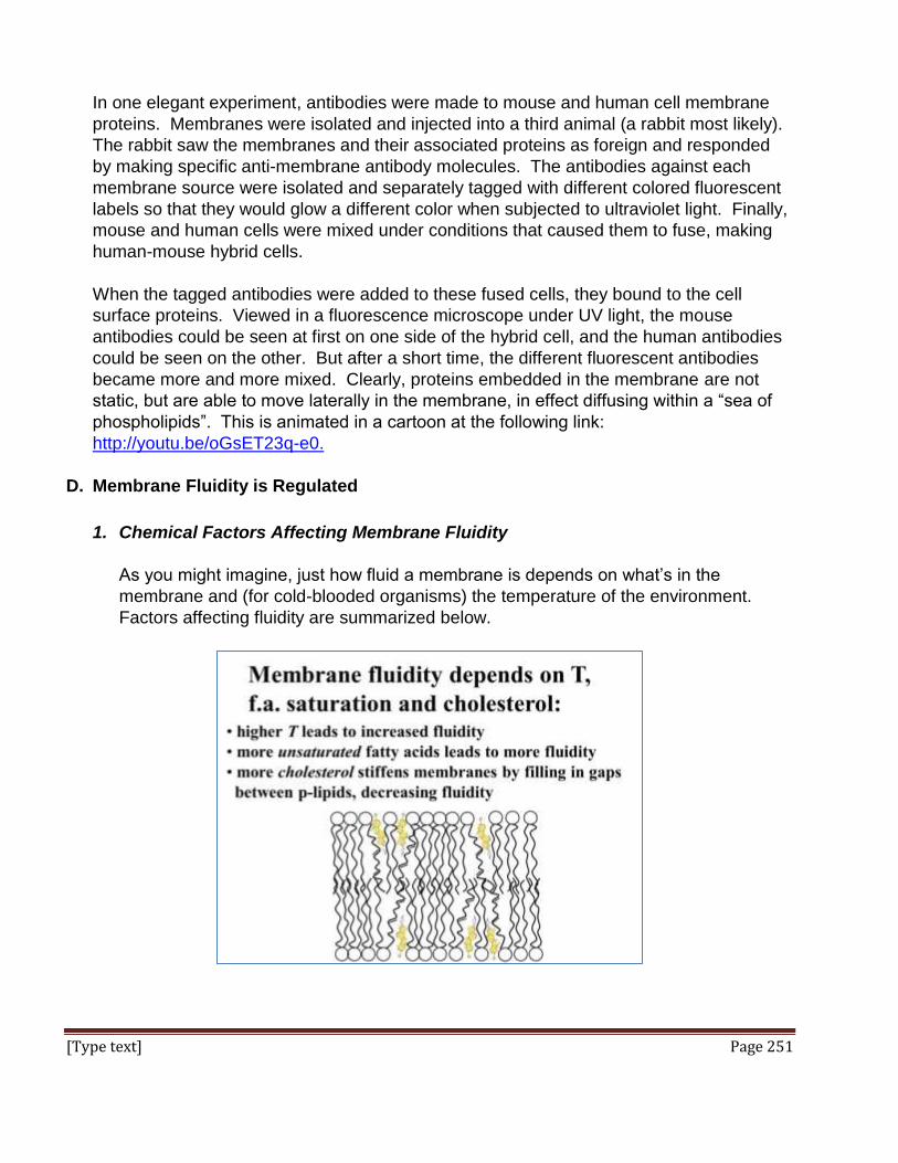
[Type text] Page 251

In one elegant experiment, antibodies were made to mouse and human cell membrane

proteins. Membranes were isolated and injected into a third animal (a rabbit most likely).

The rabbit saw the membranes and their associated proteins as foreign and responded

by making specific anti-membrane antibody molecules. The antibodies against each

membrane source were isolated and separately tagged with different colored fluorescent

labels so that they would glow a different color when subjected to ultraviolet light. Finally,

mouse and human cells were mixed under conditions that caused them to fuse, making

human-mouse hybrid cells.

When the tagged antibodies were added to these fused cells, they bound to the cell

surface proteins. Viewed in a fluorescence microscope under UV light, the mouse

antibodies could be seen at first on one side of the hybrid cell, and the human antibodies

could be seen on the other. But after a short time, the different fluorescent antibodies

became more and more mixed. Clearly, proteins embedded in the membrane are not

static, but are able to move laterally in the membrane, in effect diffusing within a “sea of

phospholipids”. This is animated in a cartoon at the following link:

http://youtu.be/oGsET23q-e0.

D. Membrane Fluidity is Regulated

1. Chemical Factors Affecting Membrane Fluidity

As you might imagine, just how fluid a membrane is depends on what’s in the

membrane and (for cold-blooded organisms) the temperature of the environment.

Factors affecting fluidity are summarized below.

[Type text] Page 252

Since higher temperatures result in more molecular motion, membrane phospholipid

and protein components of the membrane would be more fluid (move faster). Fatty

acid tails with more unsaturated C-C bonds (especially polyunsaturated fatty acids)

have more kinks, or bends. These will tend to push apart the hydrophobic tails of the

phospholipids, creating more space between them, again allowing for more movement

of membrane components. On the other hand, cholesterol molecules tend to fill the

space between fatty acids in the hydrophobic interior of the membrane, reducing the

lateral mobility of phospholipid and protein components in the membrane. In so doing,

cholesterol makes membranes less fluid and reduces membrane permeability to some

ions.

2. Functional Factors Affecting Membrane Fluidity

Evolution has adapted cell membranes to different and changing environments to

maintain the fluidity necessary for proper cell function. Cold-blooded or

poikilothermic organisms, from prokaryotes to fish and reptiles, do not regulate their

body temperatures. Thus, when exposed to lower temperatures, poikilotherms

respond by increasing the unsaturated fatty acid content of their cell membranes; at

higher temperatures, they increase membrane saturated fatty acid content. For

example, the cell membranes of fish living under the arctic ice maintain fluidity by

having high levels of both monounsaturated and polyunsaturated fatty acids. But for

fish species that range across warmer and colder environments (or that live in

climates with changing seasons) membrane composition can change to adjust fluidity.

Warm-blooded, homeothermic organisms that maintain a more or less constant body

temperature have less need to regulate membrane composition. But in an apparent

paradox, even though cells of homeotherms (mammals and birds) are in warm

internal environments, their cell membranes of have a higher ratio of polyunsaturated

fat to monounsaturated fats than say, reptiles. The resulting greater membrane fluidity

supports the higher metabolic rate of the warm-blooded species compared to

poikilotherms. Just compare the life styles of almost any mammal to a lazy alligator!

E. Making and Experimenting with Artificial Membranes

Membrane-like structures can form spontaneously. When phospholipids interact in an

aqueous environment, they aggregate to exclude their hydrophobic fatty tails from water,

forming spherical phospholipid monolayers by self-assembly, a natural aggregation of the

[Type text] Page 253

these amphipathic molecules. Called micelles, these monolayer spheres can further

self-assemble into spherical phospholipid bilayers called liposomes (below).

When they are formed in the laboratory, these structures behave somewhat like cells.

They can be centrifuged to form a pellet at the bottom of a centrifuge tube. Liposomes

can be custom designed from different kinds of phospholipids and amphipathic proteins

that become integral to the liposome membranes. And they can be made to contain

specific proteins or other molecules within the structure that cannot cross membranes.

Such were the studies that allowed the identification of the mitochondrial respiratory chain

complexes. The ability to manipulate liposome content and membrane composition make

them candidates for the drug delivery to specific cells and tissues.

F. The Plasma Membrane is Segregated into Regions with Different Properties of

Fluidity and Selective Permeability

As we will see shortly, fluidity does not result in an equal diffusion of all membrane

components around the cell membrane surface. Instead, extracellular connections

between cells as well as intracellular connections of the membrane to differentiated

regions of the cytoskeleton effectively compartmentalize the membrane into sub-regions.

Just imagine a sheet of epithelial like those in the cartoon below.

The cells expose surfaces with unique functions to the inside of the organ they line, and

one with a quite different function on the other side of the sheet. The lateral surfaces of

[Type text] Page 254

the cells are yet another membrane compartment, one that functions to connect and

communicate between the cells in the sheet. Components within a compartment may

remain fluid, but each compartment serves a unique function. This macro-differentiation

of cell membranes to permit cell-cell interactions makes intuitive sense.

The recent observation that cellular membranes are even more compartmentalized was

perhaps less anticipated. In fact, membranes are divided into micro-compartments within

which components are fluid but across which components seldom mix. Recent studies

indicate that cytoskeletal elements create and maintain these micro-discontinuities.

When integral membrane proteins are attached to cytoskeletal fibers (e.g., actin) they are

immobilized in the membrane. Furthermore, when aggregates of these membrane

proteins line up due to similar interactions, they form kind of fence, inhibiting other

membrane components from crossing. By analogy, this mechanism of micro-

compartmentalization was called the Fences and Pickets model, with the proteins

attached to the cytoskeleton serving as the pickets. The infrequent movement across the

fences was infrequent; their motion was called hop diffusion, to distinguish this motion

from the Brownian motion implied by the original fluid mosaic model.

III. Membrane Proteins (Click to see Boundless.com’s description)

Proteins may be anchored to membranes in several ways. Integral membrane proteins are

not covalently linked to membrane lipids, but because they are amphipathic, they have

hydrophobic domains that interact strongly with the fatty acid interior of membranes. Some

integral membrane proteins span the entire membrane, with hydrophilic domains facing the

cytosol or cell exterior. Peripheral proteins are held to the surface of membranes through

non-covalent interactions, and are typically dissociable from the membrane. Membrane

lipoproteins are proteins covalently linked to fatty acids in the membrane interior. These

membrane protein types are illustrated below.

[Type text] Page 255

Membrane proteins function as receptors for hormones or neurotransmitters, as antibodies,

as cell-recognition molecules that bind cells together, as cell-cell communication structures

that pass chemical information between cells, as anchors to extracellular surfaces like

connective tissue, as transporters allowing the entry into or exit of substances from cells,

even as enzymes that catalyze crucial reactions in cells. Some of these functions are

summarized and illustrated below.

Most of the functions illustrated here are performed by transmembrane proteins. However,

peripheral membrane proteins also play important roles in membrane function. Cytochrome

C in the electron transport system on the mitochondrial cristal membrane is a peripheral

protein. Other peripheral membrane proteins may serve to regulate the transport or signaling

activities of transmembrane protein complexes or may mediate connections between the

membrane and cytoskeletal elements. Peripheral membrane proteins by definition do not

penetrate membranes. They bind reversibly to the internal or external surfaces of

membranes the biological membrane with which they are associated.

[Type text] Page 256

We’ll be looking more closely at how membrane proteins are held in membranes and how

they perform their unique functions. For now, check out the table below listing major

membrane protein functions, their actions and where they act.

Basic Function Specific Actions Examples

Facilitated transport Regulate diffusion of substances

across membranes along a

concentration gradient

Ca++ & other ion channels,

glucose transporters

Active transport Use energy to move ions from low to

high concentration across membranes

Mitochondrial protein pumps,

the Na+/K+ ion pump in

neurons

Signal transduction For e.g., hormones that can’t enter

cells, these convey information from

molecular signals to cytoplasm,

leading to a cellular response

Protein hormone and growth

factor signaling,

antibody/antigen interactions,

cytokine mediation of

inflammatory responses etc.

Cell-cell interactions Cell-cell recognition and binding to

form tissues

Formation of desmosomes,

gap junctions and tight

junctions

Anchors to

cytoskeleton

Link membrane proteins to

cytoskeleton

Give cells their shape, cell

movement and response to

molecular signals

Enzymatic Usually multifunctional proteins with

enzymatic activities

The F1 ATP synthase that

uses proton gradient to make

ATP; adenylyl cyclase that

makes cAMP during signal

transduction; note that some

receptor proteins are linked to

enzymatic domains in the

cytoplasm.

[Type text] Page 257

A. How membrane proteins are held in membranes

As already noted, membrane proteins are amphipathic. The hydrophobic domain of

integral membrane proteins consists of one or more alpha-helical regions that interact

with the hydrophobic interior of the membrane, while hydrophilic domains face the

aqueous cytosol and cell exterior. Two trans-membrane proteins are cartooned below.

The protein on the left crosses the membrane once, while the one on the right crosses the

membrane three times. The locations of the N- terminus and C-terminus of a

transmembrane polypeptide are dictated by how the protein is inserted into the

membrane during synthesis and by how many times the protein crosses the membrane.

As you will see, the N-terminal end of a plasma membrane polypeptide is inserted into the

membrane such that they will always be exposed to the outside of the cell.

The alpha helical domains that anchor proteins in a membrane are mostly non-polar, and

hydrophobic themselves. As an example, consider the amino acids in the alpha-helical

domain of the red blood cell protein glycophorin A (below) that prevents red blood cells

from aggregating, or clumping in the circulation.

[Type text] Page 258

Proteins that span membranes multiple times may include amino acids with charged,

polar side chains, provided that these side chains interact between helices so that they

are shielded from the fatty acid environment in the membrane. Because of these

hydrophilic interactions, such proteins can create pores for the transport of polar

molecules and ions. Integral membrane proteins that do not span the membrane still

have a helical hydrophobic domain that anchors them in the membrane. These

membrane proteins typically interact with intracellular or extracellular molecules to hold

cells in place or otherwise give cells and tissues their structure.

The very presence of the hydrophobic alpha-helical domains in trans-membrane proteins

makes them difficult if not impossible to isolate from membranes in a biologically active

form. By contrast, the peripheral polypeptide cytochrome C readily dissociates from the

cristal membrane, making it easy to purify. For many years our understanding of the

structure and function of the mitochondrial electron transport system was limited by an

inability to purify the other biologically active electron carriers in the cristal membrane.

Hydrophobic alpha-helical domains are in fact a defining hallmark of membrane-spanning

proteins. These days, it is possible to determine the primary structure of a polypeptide

encoded by a gene even before the protein itself is discovered. For example, when the

sequence of a newly discovered polypeptide is identified following genome sequencing,

the amino acid sequence of the protein can be inferred from the coding region of the

gene. A hydrophobicity analysis of the inferred amino acid sequence can tell us if the

protein encoded by the gene is likely to be a membrane protein. Let’s look at a

hydropathy (hydrophobicity) plot (below).

[Type text] Page 259

B. Glycoproteins

Membrane proteins are often covalently linked to oligosaccharides. These

oligosaccharides are called glycans, and sugar-linked proteins are therefore called

glycoproteins. Glycoproteins are rare in the cytosol, but common on secreted proteins

and membrane proteins. The oligosaccharides are branched glycoside-linked sugars

(averaging around 15 sugar residues), typically linked via the hydroxyl group on serine or

threonine. Less frequent linkages are to modified amino acids like hydroxylysine or

hydroxyproline (O-glycosylation), and occasionally via the amide nitrogen on asparagine

(N-glycosylation). As already noted, the oligosaccharide domains of glycoproteins

typically play a major role in membrane protein function. Along with the extracellular polar

domains of integral and peripheral proteins and glycolipids, glycoproteins are a major

feature of the glycocalyx (below).

The oligosaccharides begin their synthesis in the rough endoplasmic reticulum (RER),

with the creation of a core glycoside. This partial glycan is enzymatically linked to one of

several amino acids of a membrane protein. As these proteins travel through the Golgi

vesicles of the endomembrane system, more sugars are added to the core glycoside in a

process called terminal glycosylation. The process, which explains why cells are ‘sugar

coated’ is demonstrated in the animation at this link: http://youtu.be/TkHNC8ePMPE.

Membrane glycoproteins and glycolipids enable cell-cell recognition. The O, A, B and AB

blood groups in humans are an example in which red blood cells are characterized by

different cell surface antigens that keep the cells from clumping unless mixed

inappropriately. That’s why blood is ‘typed’ before giving patients a transfusion. Other

functions include white blood cell surface antibodies that recognize foreign substances

[Type text] Page 260

(antigens) in the blood and immunoglobulins (circulating antibodies that also recognize

antigens), and cell-surface molecules of the major histocompatibility complex (MHC).

Because organs from incompatible donors will be rejected, tissue typing determines if

MHC proteins are compatible between a donor and recipient prior to an organ transplant.

Many secreted proteins (e.g., hormones) are also glycoproteins, as are those that bind to

extracellular surfaces.

C. Glycolipids

Glycolipids are phospholipids attached to oligosaccharides, and as noted, are part of the

glycocalyx. Both are only found on the extracellular surface. Glycolipids are synthesized

in much the same way as glycoproteins. Specific enzymes catalyze initial glycosylation of

either phospholipids or polypeptides, followed by the addition of more sugars.

Along with glycoproteins, glycolipids play a role in cell-cell recognition and the formation

of tissues. The glycans on the surfaces of one cell will recognize and bind to

carbohydrate receptors (lectins) on adjacent cells, leading to cell-cell attachment as well

as intracellular responses in the interacting cells. Glycoproteins and glycolipids also

mediate the interaction of cells with extracellular molecular signals and with chemicals of

the extracellular matrix (below).

[Type text] Page 261

The extracellular matrix includes components of connective tissue, basement

membranes, in fact any surfaces to which cells attach. In the next chapter we will look

more closely at the functions of membranes ad their proteins.

Some iText & VOP Key Words and Terms

amphipathic molecules glycolipids peripheral membrane

proteins

asparagine glycosylation phospholipid bilayer

cell membrane Golgi vesicles plasma membrane

cell-cell attachment Hydropathy plot poikilothermic organisms

cytoskeleton hydrophilic phosphate heads

RER

Davson–Danielli membrane model

hydrophobic fatty acid tails

Rough endoplasmic reticulum

endomembrane system hydrophobicity plot saturated fatty acids

exocytosis hydroxyproline serine

extracellular matrix (ECM) hydroxylysine temperature effects on membranes

fluid mosaic integral membrane proteins

threonine

freeze fracture method membrane asymmetry transmembrane proteins

membrane evolution membrane proteins unsaturated fatty acids

glycan N-glycosylation

glycocalyx O-glycosylation

[Type text] Page 262

Chapter 14: Membrane Function

Passive, facilitated and active transport, the traffic of proteins in cells, cell-cell

interactions, excitability and signal transduction

I. Introduction

Small molecules like O2 or CO2 can cross cellular membranes unassisted; neither the

hydrophilic surfaces nor the hydrophobic interior of the phospholipid bilayer are barriers to

their transit. On the other hand, most molecules (even water!) need the help of membrane

transport proteins to get in or out of cells and organelles. Such facilitated transport proteins

can act as gates that might be open or closed. When open, they permit diffusion of

molecules into or out of cells along a concentration gradient so that their concentrations

equalize across the membrane. Like the passive diffusion of small gasses, facilitated

diffusion does not require an input of energy. In contrast, some transport proteins are

actually pumps, using chemical energy to move molecules against a concentration gradient

by active transport so that they are at higher concentration on one side of the membrane.

For example, pumps that create sodium and potassium ion gradients are responsible for the

fact that cells are excitable. Recall that this is one of the fundamental properties of life: the

ability of cells and organisms to respond to stimuli. We’ll see such gates and pumps in action

in this chapter, as well as examples of membrane proteins involved in cell-cell interactions,

allowing their assembly into tissues and organs. We’ll also look at how cells direct proteins

appropriately to the cytoplasm, into organelles into membranes… or out of the cell. We’ll see

how membrane proteins participate in intercellular communication as well as the response of

cells to external chemical signals such as neurotransmitters, hormones, and other effector

molecules. As you read this chapter, look for how allosteric change enables regulation of the

function of membrane proteins.

Voice-Over PowerPoint Presentations

Transport Across Membranes VOP

Membrane Potential and Excitation VOP

Directing Protein Traffic in Cells VOP

Cell-Cell Communication: the Cell Surface and Cell Junctions

(Intercellular Communication: Signal Transduction VOP)

Learning Objectives

When you have mastered the information in this chapter and the associated VOPs, you

should be able to:

1. explain how and why one cell’s plasma membrane differs from that of a different cell type.

2. explain how and why the plasma membrane differs from other membranes in the cell.

[Type text] Page 263

3. determine if a solute is crossing the plasma membrane by passive or facilitated diffusion.

4. explain how salmon are able to spend part of their lives in the ocean and part swimming

upstream in freshwater to spawn without their cells shriveling of exploding!

5. explain the role of active transport in storing chemical energy (recall electron transport). 6. explain the role of active transport in maintaining or restoring a cell’s resting potential.

7. compare and contrast different kinds of gated channels.

8. describe in order the ion movements that generate an action potential.

9. compare and contrast exocytosis, pinocytosis, phagocytosis and receptor-mediated

endocytosis.

10. distinguish between signal molecules that enter cells to deliver their chemical message

and those deliver their message only to the plasma membrane.

11. trace an intracellular response to a steroid hormone to its most likely cellular effect.

12. trace the response of a liver cell to adrenalin from the plasma membrane to the

breakdown of glycogen.

13. compare the signal transduction activities of different G-protein receptors leading to the

first active kinase enzyme.

14. explain the molecular basis of a liver cells identical response to two different hormones

(i.e., adrenalin and glucagon).

15. Describe/explain how a phosphorylation cascade amplifies a cellular response to a small

amount of an effector (signal) molecule.

16. discuss the difference and interactions between the glycocalyx, basement membrane and

extracellular matrix (ECM).

17. explain the functions of the ECM and identify components involved in those functions.

18. describe how the molecular structure of fibronectin supports its different functions.

19. speculate about the structural relationship between cell surface and the cytoskeleton.

20. compare and contrast the structures and functions of the different cell junctions.

21. distinguish between the structures and functions of cadherins, clathrin, COPs, adaptin,

selectins, SNAREs and CAMs.

22. state an hypothesis to explain why some cancer cells divide without forming a tumor.

II. Membrane Transport

Molecules move in and out of cells in one of 3 ways: passive diffusion, facilitated

transport and active transport. The first two release free energy; active transport

consumes it. The first control on the passage of molecules across membranes is the semi-

permeable character of the membrane itself. Only a few small relatively uncharged

molecules can cross a membrane unassisted (i.e., by passive diffusion). And only specific

hydrophilic molecules are allowed to cross cellular membranes. That specificity resides in

the integral membrane proteins of facilitated transport and active transport. For a long

time, water was thought by many to cross membranes unassisted. And indeed it does so…

[Type text] Page 264

to a limited extent. But water is a small and highly charged polar covalent molecule, and

some suspected that water would require an assist to get across membranes efficiently. We

now know that most water, just like most solutes, crosses membranes by facilitated diffusion.

As you may imagine, the molecular movement into or out of cells is further controlled by

allosteric regulation of these proteins. Shortly, we’ll consider water transport as a special

case of facilitated diffusion of a solvent rather than solutes. First, let’s look at passive

diffusion.

A. Passive Diffusion

Passive diffusion is the movement of molecules over time by random motion from regions

of higher concentration to regions of lower concentration. Diffusion of solutes in a

solution is illustrated in this link: http://youtu.be/1PPz5kzOChg. Significant passive

diffusion across cellular membranes is limited to a few molecules, like gasses (O2, CO2,

N2…) that can freely cross the hydrophobic phospholipid barrier. The rapid diffusion of

these gasses is essential during physiological respiration when O2 and CO2 exchange

between the alveolar capillaries and cells of the lungs, and during cellular respiration in

mitochondria. Diffusion across membranes does not require energy. In fact, diffusion

across membranes releases energy - recall the movement of protons thought the F1

ATPase proton gate linked to ATP synthesis during oxidative phosphorylation. As

suggested in the animation, the diffusion of a molecule is determined by its own

concentration; it is unaffected by the concentration of other molecules. Over time,

random motion of solutes within and across compartments results in a dynamic

equilibrium for each different solute over time. At equilibrium, solute molecules continue to

diffuse across the membrane but for each molecule moving across in one direction,

another molecule of the same solute crosses in the other direction.

B. Facilitated Diffusion of Solutes and Ions

Facilitated diffusion is the spontaneous (downhill) passage of molecules or ions across a

biological membrane passing through specific transmembrane proteins. The difference

between passive and facilitated diffusion is easily seen in the kinetics of each. Recall that

the rate of enzyme catalysis is saturable. That is, as the concentration of substrate is

increased, the rate of the catalyzed reaction approaches a maximum (Vmax), when all

enzyme molecules in solution are bound to substrate molecules. The same saturation

phenomenon applies to facilitated transport – the rate of solute movement across a

membrane is directly proportional to the number of transport proteins in the membrane.

[Type text] Page 265

The kinetics of passive and facilitated diffusion can be measured and graphed as shown

below.

There are three kinds of facilitated transport of solutes (below).

The GLUT protein (glucose transporter) protein illustrated above (left) allows glucose

uniport, the specific transport of a single substance in or out of cells. Other glucose

transport proteins couple the simultaneous movement of glucose and sodium ions into

cells, an example of symport (above center). Molecules can also be exchanged across

[Type text] Page 266

membranes by antiport (above right). In this example, ATP crosses the cristal

membrane out of the mitochondrial matrix at the same time as ADP enters the matrix.

Whether by uniport, symport or antiport, solutes independently cross membranes from

regions where each is at high concentration to cellular compartments where each is at

lower concentration. Recall that diffusion proceeds with a release of free energy, the

amount being dependent on the concentrations of the solutes. The difference between

uniport of glucose and symport of glucose and sodium ions is animated at

http://youtu.be/OEFUvF56deU.

Proteins mediating facilitated diffusion include carrier proteins and channel proteins.

Carrier proteins allow solute transport while channel proteins are essentially ion pores;

with their high charge-to-mass ratio, ions cannot freely cross the hydrophobic membrane

barrier. Both carrier and channel proteins undergo allosteric change during transport.

They are also typically subject to allosteric regulation, rather than being in a constant

‘open’ state. Click http://youtu.be/SXL1RBK3Rm8 to compare passive and facilitated

diffusion. Examples of facilitated diffusion are considered in further detail below.

1. Carrier Proteins

Carrier proteins undergo allosteric change when they bind to a solute to be

transported. As the solute is transported, the carrier protein undergoes a second

conformational change, so that when the solute reaches the other side of the

membrane, it no longer has a high affinity for the carrier protein. Upon release of the

solute after transport, a final allosteric change restores the shape of the transport

protein (below).

Any given carrier protein is specific for a single solute, or at most a single family of

closely related solutes. We just saw the GLUT1 transporter carrier protein that allows

glucose (but not fructose or ribose!) to cross cell membranes. Specific carrier proteins

[Type text] Page 267

also facilitate the transport of amino acids and other charged solutes across cell

membranes. Once again, carrier proteins can be allosterically regulated by molecules

inside or outside of cells that are indicators of cell status, i.e., their need to take up or

release a particular solute. A perfect example is the regulation of glucose transport

into cells by insulin. One of the consequences of insulin released during a meal (or

even just in anticipation of a meal) stimulates glucose transporters to take up glucose.

Type II (adult onset) diabetes is in part caused by an inability of those transporters to

respond to insulin.

Now for that special case! Most water gets across membranes by facilitated diffusion

using aquaporins. Small amount of water can cross the phospholipid bilayer

unassisted or incidentally when ions flow through their channel proteins. Butt

aquaporins are required to facilitate diffusion of water across membranes at high

rates. Some aquaporins only transport water. Others have evolved to co-facilitate the

transport of glucose (see above), glycerol, urea, ammonia and carbon dioxide and

even ions (protons) along with water. Like other carrier proteins, aquaporins are

allosterically regulated to allow cells to meet their specific water balance requirements.

So fundamental was the understanding of water balance that the discovery of

aquaporins earned Peter Agre a Nobel Prize in Chemistry in 2003.

Since Agre’s discovery (in 1992), several genetic diseases have been linked to

mutations in aquaporin genes. One is a rare form of diabetes in which the kidneys

excrete abnormally large volumes of water; kidney cells are critically involved in

vertebrate water balance and contain large amounts of aquaporins in their

membranes. Another example involves mutations in aquaporin genes that lead to the

development of cataracts in both eyes. Since their initial discovery in red blood cells

in 1992, aquaporins have been found in bacteria and plants. See more about

aquaporin research at http://en.wikipedia.org/wiki/Aquaporin. Learn more about the

osmosis shortly.

2. Ion Channels

Ion homeostasis in blood and extracellular fluids is tightly controlled, often within very

narrow limits, by allosteric regulation of ion channel proteins. Ion channels are often

formed from more than one integral membrane protein. When stimulated, channel

proteins rearrange to open a polar pore to allow specific ion transport. Some ion

channels (like the glucose/sodium ion symport system noted above) mobilize the

energy of diffusion to co-transport an ion with another solute through a carrier protein.

Ion channels are also responsible for the excitability of cells, where Na+ , K+ and Ca++

channels collaborate in ion movements into and out of cells leading to neuronal or

muscle cell responses (more shortly!).

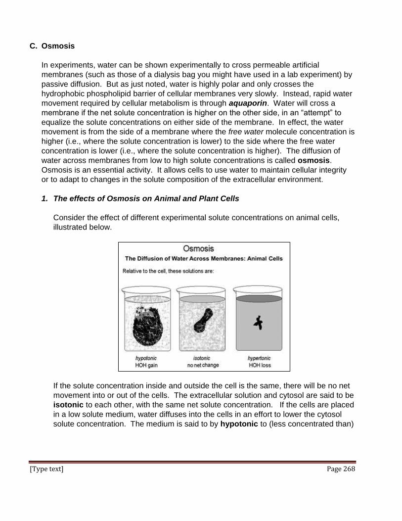
[Type text] Page 268

C. Osmosis

In experiments, water can be shown experimentally to cross permeable artificial

membranes (such as those of a dialysis bag you might have used in a lab experiment) by

passive diffusion. But as just noted, water is highly polar and only crosses the

hydrophobic phospholipid barrier of cellular membranes very slowly. Instead, rapid water

movement required by cellular metabolism is through aquaporin. Water will cross a

membrane if the net solute concentration is higher on the other side, in an “attempt” to

equalize the solute concentrations on either side of the membrane. In effect, the water

movement is from the side of a membrane where the free water molecule concentration is

higher (i.e., where the solute concentration is lower) to the side where the free water

concentration is lower (i.e., where the solute concentration is higher). The diffusion of

water across membranes from low to high solute concentrations is called osmosis.

Osmosis is an essential activity. It allows cells to use water to maintain cellular integrity

or to adapt to changes in the solute composition of the extracellular environment.

1. The effects of Osmosis on Animal and Plant Cells

Consider the effect of different experimental solute concentrations on animal cells,

illustrated below.

If the solute concentration inside and outside the cell is the same, there will be no net

movement into or out of the cells. The extracellular solution and cytosol are said to be

isotonic to each other, with the same net solute concentration. If the cells are placed

in a low solute medium, water diffuses into the cells in an effort to lower the cytosol

solute concentration. The medium is said to by hypotonic to (less concentrated than)

[Type text] Page 269

the cytosol. Under hypotonic conditions animal cells will swell and burst. If the cells

are placed in a hypertonic solution (one with a higher solute concentration than the

cytosol) water leaves the cell and the cells shrivel up. From this brief description you

can conclude that water crosses from the hypotonic to the hypertonic side of a

membrane.

Exposure of plant cells to hypotonic or hypertonic solutions has similar effects on

water movement across cell membranes. However, cell walls limit how much a plant

cell can swell, and shriveling looks different because the cell membrane is actually

attached to the cell wall! Thus, water entering plant cells in hypotonic media moves

from the cytosol into water vacuoles called tonoplasts. This results in higher

osmotic pressure (water pressure) in the tonoplasts, and therefore in the cytosol,

thus pushing against the cell membrane. Rather than bursting, the cell membrane

pushes against cell walls causing the cells and plant tissues to stiffen, or become

turgid. The pressure against plant cell walls is called turgor pressure. You will have

encountered this phenomenon if you ever over-watered house plants; the stiffened

leaves and stems become brittle and are easily snapped or broken. As you might

guess, water cannot enter plant cells indefinitely, even in hypotonic solutions. Instead,

water stops entering the cells when the osmotic pressure outside the cells and the

turgor pressure inside the cells are at equilibrium. The effects of hypertonic and

hypotonic solutions on plant cells are illustrated below.

Plant cell membranes are actually attached to the cell wall at plasmodesmata,

structures that connect the plasma membranes of adjacent cells through their cell

walls, allowing them to directly share chemical information. So, when plant cells lose

water in a hypertonic solution, they undergo plasmolysis, membrane shrinkage while

maintaining cell wall attachments. You may have seen under-watered plants with

floppy or droopy stems and leaves. These have become flaccid because the turgor

pressure is insufficient to keep the leaves and stems upright.

[Type text] Page 270

Normally, plant cells require a continual supply of water for use in photosynthesis (to

provide hydrogen to reduce CO2 to glucose) and because excess water is lost from

plant tissues (especially leaves) by transpiration. The use and loss of water lowers

cellular osmotic pressure. As water moves up from the roots to replace water used

and lost by leaf cells, the osmotic pressure drops in the fine root hair cells (with their

high surface area). This draws water into the cells and roots by osmosis. Thus

osmotic pressure is the main force driving water into plants and, defying gravity, up

from the roots to the rest of the plant.

Formally, osmotic or turgor pressure is defined as the force per unit area (pressure)

required to prevent the passage of water across a semipermeable membrane from a

hypotonic to a hypertonic solution.

2. Osmotic Pressure and Osmoregulation

Changes in osmotic environment can stress or kill an organism. For example,

freshwater organisms (protozoa or fish) placed in sea water will die. Likewise salt-

water fish placed in freshwater. However, organisms can osmoregulate, or control

the osmotic pressure in their cells, at least to a point. Take Paramecium for example.

Water constantly enters these freshwater protists because the solute concentration in

the cytosol is always higher than the freshwater water they live in. To cope with a

constant uptake of water, the cells contain contractile vacuoles that collect excess

water and then contract to expel the water.

At a high energy cost, Paramecia constantly pump water out of the cell to maintain

water balance (i.e., correct osmotic pressure). Larger organisms like freshwater fish

cope with their hypotonic environment by urinating a lot!

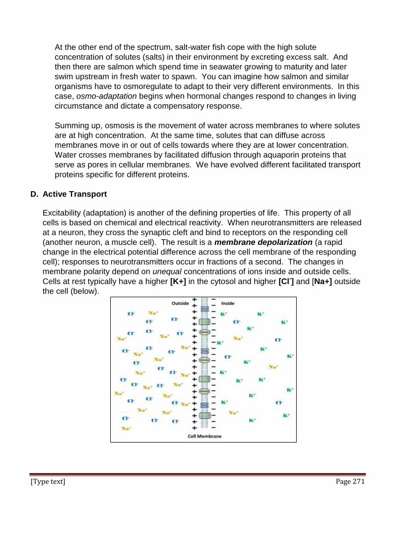
[Type text] Page 271

At the other end of the spectrum, salt-water fish cope with the high solute

concentration of solutes (salts) in their environment by excreting excess salt. And

then there are salmon which spend time in seawater growing to maturity and later

swim upstream in fresh water to spawn. You can imagine how salmon and similar

organisms have to osmoregulate to adapt to their very different environments. In this

case, osmo-adaptation begins when hormonal changes respond to changes in living

circumstance and dictate a compensatory response.

Summing up, osmosis is the movement of water across membranes to where solutes

are at high concentration. At the same time, solutes that can diffuse across

membranes move in or out of cells towards where they are at lower concentration.

Water crosses membranes by facilitated diffusion through aquaporin proteins that

serve as pores in cellular membranes. We have evolved different facilitated transport

proteins specific for different proteins.

D. Active Transport

Excitability (adaptation) is another of the defining properties of life. This property of all

cells is based on chemical and electrical reactivity. When neurotransmitters are released

at a neuron, they cross the synaptic cleft and bind to receptors on the responding cell

(another neuron, a muscle cell). The result is a membrane depolarization (a rapid

change in the electrical potential difference across the cell membrane of the responding

cell); responses to neurotransmitters occur in fractions of a second. The changes in

membrane polarity depend on unequal concentrations of ions inside and outside cells.

Cells at rest typically have a higher [K+] in the cytosol and higher [Cl-] and [Na+] outside

the cell (below).

[Type text] Page 272

Thus cells have a resting potential, typically about -50mv to -70mv, shown here as a

difference in charge or potential difference across the membrane. Membrane

depolarization in responsive cells (neuron, muscle) results in a flow of ions, as does the

e.g., the ion-assisted symport of glucose already noted. And, while not subject to ion flow

mediating a specific cellular function, the ion gradients sustaining a cellular resting

potential are slowly disturbed by a slow leakage across membranes otherwise

impermeable to ions. Whether by a dramatic depolarization or other utilitarian ion flow or

just ion leakage, cells must expend energy to restore cellular ion concentrations. The

maintenance of a correct balance of ions requires the active transport of these ions

across the membrane. This energetically unfavorable process requires an input of free

energy. ATP hydrolysis provides the energy for operation of a Na+/K+ pump, an active

transport protein complex linked to ATPase activity. Jens C. Skou discovered the Na+/K+

pump in 1950 and received a Nobel Prize in 1997 in recognition of the importance of our

understanding of ion movements across cell membranes. We will consider ion flow

during cell excitation and at how ion pumps work. Let’s begin by looking at how a Na+/K+

pump works to restore and maintain ion gradients.

Refer to the animation at this link as you read: http://youtu.be/-xZvya2Gt50. From the

video at this link you see that as ATP is hydrolyzed by the ATPase domain of the Na+/K+

pump, the hydrolyzed phosphate attaches to the pump. This results in a allosteric change

allowing the pump to bind 3 Na+ ions. Binding of the Na+ ions causes a second

conformational change causing release of the Na+ ions into the extracellular fluid. In this

new conformation, two K+ ions from the extracellular fluid bind to the pump protein. K+

binding causes the hydrolysis of the phosphate from the pump protein, along with a final

allosteric change allowing the release of the two K+ ions into the cytosol. Returned to its

starting shape, the Na+/K+ pump is ready for action again.

III. Ligand and Voltage Gated Channels at Work in Neurotransmission.

A. Measuring Ion Flow and Membrane Potential

When a neurotransmitter binds to receptors on a responding cell (e.g., another neuron, a

muscle cell), ligand-gated ion channels open, allowing an influx of Na+ ions, thereby

disrupting the resting potential of the target cell. The effect is only transient if the

membrane potential remains negative. But if enough Na+ ions enter the cell, the

membrane is depolarized and can become hyperpolarized, causing a localized reversal

of normal membrane polarity (say from –70 mV to +65mV or more). Hyperpolarization

generates an action potential that will travel like a current along the neural or muscle cell

membrane, eventually triggering a physiological response, e.g., the excitation of the next

nerve cell in a neuronal pathway or contraction of the muscle cell.

[Type text] Page 273

Ion flow across a cell membrane can be detected using the patch-clamp technique,

illustrated below:

The patch-clamp technique reveals a correlation between ion movements during the

generation of an action potential, as illustrated below.

An action potential (in fact any degree of shift from resting potential) involves facilitated

diffusion of specific ions into or out of the cell through specific gated ion channels that

must open and close in sequence. You can see from this illustration that active transport

will not be necessary for restoring the resting potential, at least not directly. The cell can

continue to respond to stimuli with action potentials… for as long as there is sufficient Na+

outside the cell and K+ inside the cell.

[Type text] Page 274

The ATP-dependent Na+/K+ pump does participates indirectly to restore the resting

potential across membranes by restoring the appropriate Na+-K+ balance across the

responding cell membrane. After a nerve or muscle cell fires once or several times, the

[K+] inside the cell and the [Na+] outside the cell would drop to a point where the cell can’t

fire again… were it not for the operation of Na+/K+ pumps. Each cycle of pumping

exchanges 3 Na+ ions from the intracellular space for 2 K+ ions from the extracellular

space. The pump has three effects:

It restores sodium concentrations in the extracellular space relative to the cytoplasm.

It restores potassium concentrations in the cytoplasm relative to the extracellular

space.

Together with the higher Cl- ion concentration in the cytosol, the unequal exchange of

Na+ for K+ ions maintains the resting potential of the cell.

B. Ion Channels in Neurotransmission

The initial membrane depolarization phase of an action potential results from an orderly,

sequential response of voltage-gated and ligand-gated channels in the signaling neuron.

In a responding muscle cell, membrane ion channels will either open upon electrical

stimulation or by binding of a chemical ligand (the neurotransmitter). The cooperation of

different gated channels at a neuromuscular junction is illustrated below:

See this process animated at this link: http://youtu.be/tSks9WPDxHM

[Type text] Page 275

As you can see from the illustration, two kinds of channels are at work here, ligand-gated

channels and voltage-gated channels. After a neuron fires, an electrical impulse (a

moving region of hyperpolarization) travels down the axon to the nerve ending, where this

transient charge difference across the cell membrane (an electrical potential) stimulates a

Ca++-specific voltage-gated channel to open. Ca++ ions then flow into the cell because

they are at higher concentrations in the synaptic cleft than in the cytoplasm. The Ca++

ions cause release of neurotransmitters into the synaptic cleft. The neurotransmitters

bind to a receptor on the responding cell plasma membrane. This receptor is a ligand-

gated channel (also called a chemically-gated channel). Upon binding of the ligand

(neurotransmitter) the channel protein opens, allowing rapid diffusion of Na+ ions into the

cell, creating the action potential that leads to the cellular response, in this case, muscle

contraction. We have already seen that K+ channels participate in restoring membrane

potential after an action potential. We’ll look later at the cellular events, including more

ion flux and pumping involved in contraction.

IV. Endocytosis and Exocytosis

Endocytosis is a mechanism for internalizing extracellular substances, usually large

molecules like proteins, or insoluble particles or microorganisms. Exocytosis is the

secretion of large molecules (proteins and glycoproteins) from cells into the extracellular fluid.

Exocytosis also places proteins made by cells onto the cell surface.

A. Endocytosis

The three main kinds of endocytosis are summarized below.

[Type text] Page 276

1. Phagocytosis (above left): Phagocytes extend pseudopodia by membrane

evagination. The pseudopodia of amoeba (and amoeboid cells generally) engulf

particles of food that end up in digestive vesicles (phagosomes) inside the cytosol.

Phagocytes, a class of white blood cells that are part of our immune system, engulf

foreign particles that must be eliminated from the body. Engulfed particles are

digested when a lysosome fuses with the phagosome, activating stored hydrolytic

enzymes. Phagocytosis is initiated when particles are detected at the outer cell

surface.

2. Pinocytosis (above center): Pinocytosis is a non-specific, more or less constant

pinching off of small vesicles that engulfs extracellular fluid containing solutes; they

are too small to include significant particulates.

3. Receptor-mediated endocytosis (above right): Receptor-mediated endocytosis

relies on the affinity of receptors for specific extracellular substances that must be

internalized by the cell. Upon binding their ligands, the receptors aggregate in

differentiated regions of cell membrane called coated pits. The coated pits then

invaginate and pinch off to form a coated vesicle. The contents of the coated vesicle

are eventually delivered to their cellular destinations, after which their membranes are

recycled to the plasma membrane. As receptor-mediated endocytosis is perhaps the

best understood mechanism for bringing larger substances into cells, let’s take a

closer look…

The electron micrograph series below illustrates the invagination of coated pits to form

clathrin-coated vesicles; the receptor and coat proteins are clearly visible as large

particles!

[Type text] Page 277

Clathrin, a large protein, is linked to specific integral membrane proteins via adaptor

protein 1 (AP1). While clathrin is the principal protein on the surface of the

invaginated coated pit, AP1 recruits specific cargo proteins to be brought into the cell

when the coated pits invaginate. Some details of receptor-mediated endocytosis is

illustrated below.

As the illustration shows, substances to be internalized bind to receptors on the cell

membrane that then cluster to form a coated pit. Assisted by the protein dynamin (a

GTPase), the coated pits invaginate. The final pinching off of a coated vesicle

required GTP hydrolysis.

Once internalized, the coated vesicles lose their clathrin and associated adaptor

protein coat. The uncoated vesicle fuses with an early endosome to form a sorting

vesicle that separates imported content from the receptors that are recycled to the

membrane. In the vesicle that remains, now called a lysosome, digestive enzymes

catalyze hydrolysis of the vesicle contents which are released for cellular use.

Adaptor protein

[Type text] Page 278

A major example of receptor-mediated endocytosis is the uptake of cholesterol bound

to low density lipoprotein (LDL), a complex of phospholipid, protein and cholesterol

illustrated below.

As many as 15,000 molecules of cholesterol can be carried by a single LDL complex.

LDL is sometimes called “bad cholesterol” because it is not good for you when it is too

high, compared to high-density lipoprotein (HDL), often called “good cholesterol”.

B. Exocytosis

Maintaining cell size or volume seems to be a built-in component of the machinery of

receptor-mediated endocytosis. However, exocytosis is necessary to restore plasma

membrane internalized by pinocytosis and phagocytosis, and for eliminating cellular

[Type text] Page 279

waste products. Exocytosis is also the end-point of a complex process of packaging

proteins destined to be secreted from the cell or to be membrane proteins themselves.

Below is a more detailed summary pathways shared by exocytosis and endocytosis,

including the formation of lysosomes, secretion vesicles and similar organelles, along with

the fate of endocytosed particles whose molecular components will be digested and used

by the cell.

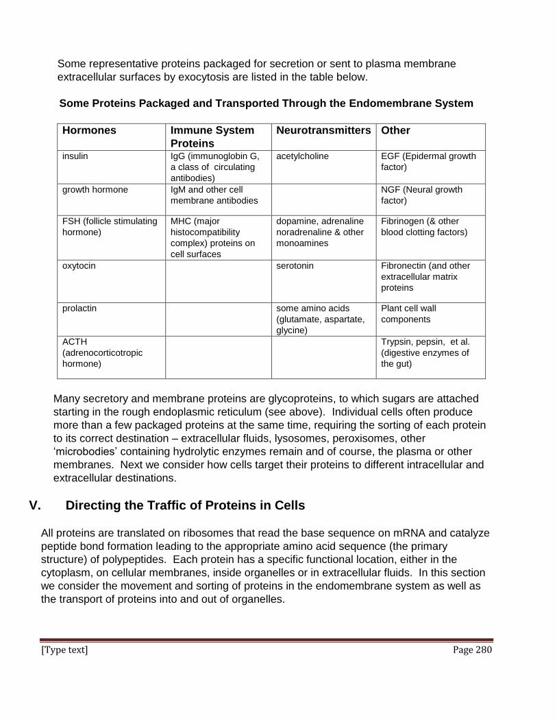
[Type text] Page 280

Some representative proteins packaged for secretion or sent to plasma membrane

extracellular surfaces by exocytosis are listed in the table below.

Some Proteins Packaged and Transported Through the Endomembrane System

Hormones Immune System

Proteins

Neurotransmitters Other

insulin IgG (immunoglobin G,

a class of circulating

antibodies)

acetylcholine EGF (Epidermal growth

factor)

growth hormone IgM and other cell

membrane antibodies

NGF (Neural growth

factor)

FSH (follicle stimulating

hormone)

MHC (major

histocompatibility

complex) proteins on

cell surfaces

dopamine, adrenaline

noradrenaline & other

monoamines

Fibrinogen (& other

blood clotting factors)

oxytocin serotonin Fibronectin (and other

extracellular matrix

proteins

prolactin some amino acids

(glutamate, aspartate,

glycine)

Plant cell wall

components

ACTH

(adrenocorticotropic

hormone)

Trypsin, pepsin, et al.

(digestive enzymes of

the gut)

Many secretory and membrane proteins are glycoproteins, to which sugars are attached

starting in the rough endoplasmic reticulum (see above). Individual cells often produce

more than a few packaged proteins at the same time, requiring the sorting of each protein

to its correct destination – extracellular fluids, lysosomes, peroxisomes, other

‘microbodies’ containing hydrolytic enzymes remain and of course, the plasma or other

membranes. Next we consider how cells target their proteins to different intracellular and

extracellular destinations.

V. Directing the Traffic of Proteins in Cells

All proteins are translated on ribosomes that read the base sequence on mRNA and catalyze

peptide bond formation leading to the appropriate amino acid sequence (the primary

structure) of polypeptides. Each protein has a specific functional location, either in the

cytoplasm, on cellular membranes, inside organelles or in extracellular fluids. In this section

we consider the movement and sorting of proteins in the endomembrane system as well as

the transport of proteins into and out of organelles.

[Type text] Page 281

A. Packaging proteins in the RER

All proteins begin synthesis in the same way, with the formation of an initiation complex

and subsequent elongation cycles of carboxy terminal growth by amino acid

addition. But secretory proteins and proteins destined for lysosomes, peroxisomes or

other microbodies complete elongation directly into the RER cisternae.

An early experiment showed that secreted polypeptides made in an in vitro translation

system were larger (longer) than the same polypeptides isolated from secretion fluids. In

this experiment, mRNA was isolated from a mouse myeloma (cancer) cell line that

synthesized an easily identified immunoprotein, the IgG light chain. The cells were

allowed to grow in media containing radioactive amino acid precursors so that they would

secrete radioactive IgG light chain. mRNA was extracted from another batch of myeloma

cells and mixed with a cell-free translation system also containing radioactive amino

acids. The proteins made in vivo and those translated in vitro were compared side by

side on electrophoretic gels that separate proteins by molecular weight (effectively

equivalent to polypeptide length). As detected by autoradiography after electrophoresis,

the radioactive polypeptide synthesized in vitro migrated more slowly on the gel than the

mature, secreted polypeptide, meaning that the cell-free translation product was larger

than the mature secreted polypeptide. This experiment is summarized below.

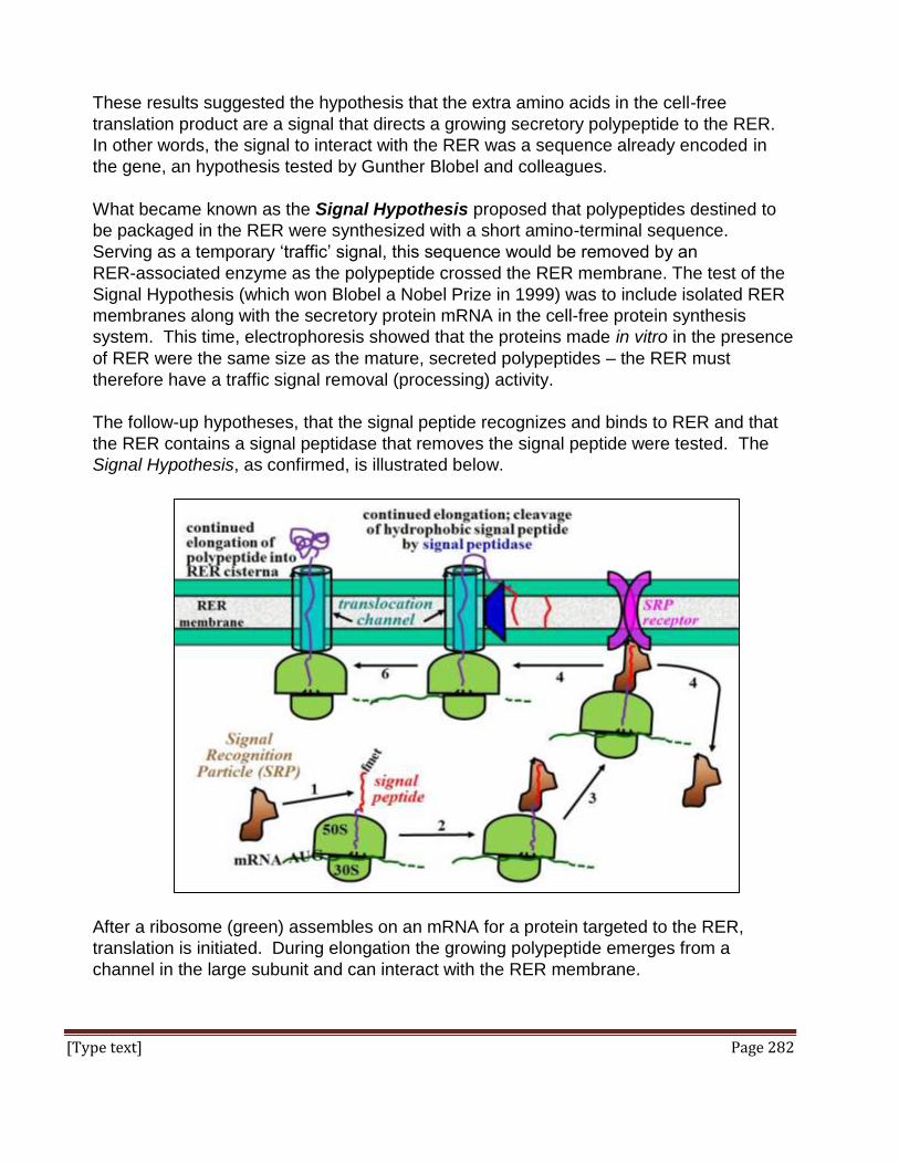
[Type text] Page 282

These results suggested the hypothesis that the extra amino acids in the cell-free

translation product are a signal that directs a growing secretory polypeptide to the RER.

In other words, the signal to interact with the RER was a sequence already encoded in

the gene, an hypothesis tested by Gunther Blobel and colleagues.

What became known as the Signal Hypothesis proposed that polypeptides destined to

be packaged in the RER were synthesized with a short amino-terminal sequence.

Serving as a temporary ‘traffic’ signal, this sequence would be removed by an

RER-associated enzyme as the polypeptide crossed the RER membrane. The test of the

Signal Hypothesis (which won Blobel a Nobel Prize in 1999) was to include isolated RER

membranes along with the secretory protein mRNA in the cell-free protein synthesis

system. This time, electrophoresis showed that the proteins made in vitro in the presence

of RER were the same size as the mature, secreted polypeptides – the RER must

therefore have a traffic signal removal (processing) activity.

The follow-up hypotheses, that the signal peptide recognizes and binds to RER and that

the RER contains a signal peptidase that removes the signal peptide were tested. The

Signal Hypothesis, as confirmed, is illustrated below.

After a ribosome (green) assembles on an mRNA for a protein targeted to the RER,

translation is initiated. During elongation the growing polypeptide emerges from a

channel in the large subunit and can interact with the RER membrane.

[Type text] Page 283

From the illustration above, the steps of the process are:

1. Elongation results in the extension of a signal sequence (signal peptide) beyond the

confines of the large ribosomal subunit. The signal peptide is a mostly hydrophobic

region at the N-terminus of the growing chain.

2. An SRP (signal recognition particle) binds to the amino-terminal hydrophobic signal

peptide.

3. Translation is then arrested until the SRP-ribosome complex finds the RER

membrane.

4. The ribosome-SRP complex binds SRP receptor on the RER membrane and the SRP

detaches from the growing polypeptide chain. The SRP is recycled).

5. Translation elongation resumes through a translocation channel.

6. A signal peptidase enzyme in the RER membrane recognizes and catalyzes co-

translational hydrolysis of the signal peptide, which remains embedded in the RER

membrane.

7. Elongation continues; the growing polypeptide begins to fold in the RER.

B. Synthesis of Membrane-Spanning (Integral) Proteins

N-terminal signal sequences also guide integral proteins to the RER. But a stop-transfer

sequence (hydrophobic domain within the polypeptide chain) traps the protein in the fatty

acid interior of the membrane. Multiple stop-transfer sequences result in transmembrane

proteins that span a membrane more than once (below)

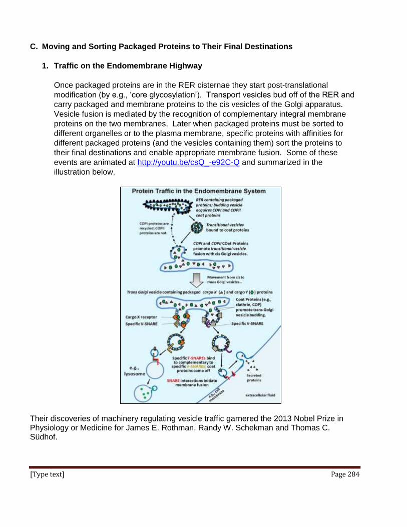
[Type text] Page 284

C. Moving and Sorting Packaged Proteins to Their Final Destinations

1. Traffic on the Endomembrane Highway

Once packaged proteins are in the RER cisternae they start post-translational

modification (by e.g., ‘core glycosylation’). Transport vesicles bud off of the RER and

carry packaged and membrane proteins to the cis vesicles of the Golgi apparatus.

Vesicle fusion is mediated by the recognition of complementary integral membrane

proteins on the two membranes. Later when packaged proteins must be sorted to

different organelles or to the plasma membrane, specific proteins with affinities for

different packaged proteins (and the vesicles containing them) sort the proteins to

their final destinations and enable appropriate membrane fusion. Some of these

events are animated at http://youtu.be/csQ_-e92C-Q and summarized in the

illustration below.

Their discoveries of machinery regulating vesicle traffic garnered the 2013 Nobel Prize in Physiology or Medicine for James E. Rothman, Randy W. Schekman and Thomas C. Südhof.

[Type text] Page 285

Let’s follow some proteins in and on RER membranes through the cell:

Transition vesicles carrying their mix of packaged proteins bud off of RER with

the help of COP (Coat Proteins). Transition vesicles are smooth, having lost the

ribosomes that characterize RER.

These vesicles fuse with the cis Golgi vesicles, a process also mediated by COP

proteins. COPI proteins detach during or after fusion to be recycled back to the

RER

.

Packaged proteins and membrane proteins are further processed as the pass

through the Golgi vesicle stack, for example undergoing terminal glycosylation.

At the trans face of the Golgi vesicles, cargo receptor proteins in the membranes

begin to bind specific packaged proteins (now called cargo proteins). With the

help of clathrin and other COP proteins, cargo protein-bound receptor proteins

bud off from the trans Golgi stack. But this time, specific cargo proteins are

sequestered in separate vesicles as they are sorted to different destinations.

These budding vesicles also acquire membrane V-SNARE (for vesicle-SNARE)

proteins.

When V-SNARE proteins on their vesicles bind to T-SNARE (for target SNARE)

proteins on receiving membranes, the membranes fuse.

o Some vesicles follow this pathway, fusing with lysosomes or similar vesicles to

stock them with appropriate enzymes and other protein content. Coat proteins

come off of the fusing vesicle and are recycled while the vesicle contents are

transferred.

o Vesicles containing proteins to be secreted typically fuse to form larger

secretory vesicles. Secretory vesicles can be stored until the cells are

signaled to release their contents from the cell. At that point, secretion vesicles

fuse with the plasma membrane, releasing their contents to the extracellular

fluid. Once again, coat proteins and clathrin come off of the secretory vesicle

during fusion.

Other players have been left out of this discussion, notably those that hydrolyze

nucleotide triphosphates to provide the energy for this protein trafficking. Perhaps it

should be no surprise that some of the molecular players in controlling protein traffic

also have a role in receptor-mediated endocytosis (e.g., clathrin). After all,

endocytosis is at least partly, molecular traffic in the opposite direction of vesicle

formation and secretion.

[Type text] Page 286

1. Nuclear Protein Traffic

Almost all proteins are encoded in the nucleus and translated in the cytosol, including

most of those found in nuclei, mitochondria and chloroplasts (see the Endosymbiotic

Hypothesis for a description of intra-organelle gene expression). Proteins

synthesized in the cytosol destined for these organelles contain oligopeptide traffic

signals that direct them to their appropriate destinations.

We saw earlier that large molecules (mRNAs, tRNAs) and even whole particles (i.e.,

ribosomal subunits) cross the nuclear envelope through nuclear pores. As for proteins

headed for the nucleus, a nuclear localization signal rich in positively charged amino

acids (lysine, proline) enables binding to a negatively charged domain in a nuclear

transport receptor protein in the cytosol (below).

As the complex of the two proteins approach a nuclear pore it interacts with nuclear

pore fibrils, causing the pore to open. The two bound proteins cross the double

membrane of the nuclear envelope, accumulating against a concentration gradient.

The active transport comes from ATP hydrolysis as the nuclear proteins enter the

nucleus as animated at http://youtu.be/vgZHf_Ju-PQ.

[Type text] Page 287

3. Mitochondrial Protein Traffic

Recall that mitochondria contain their own genome and translational machinery,

transcribing their own RNAs and translating their own proteins. However, many

mitochondrial proteins are encoded by nuclear genes. These proteins are synthesized

with an N-terminal signal sequence which binds to a receptor protein that spans

both the mitochondrial outer membrane (OM) and cristal membrane (CM), as

illustrated below.

The receptor protein delivers the protein to membrane contact proteins that also

span both mitochondrial membranes. The membrane contact proteins serve as a

pore through which the protein crosses into the mitochondrial matrix. However, unlike

the co-translational packaging of proteins by the RER, mitochondrial protein transfer is

post-translational and involves a so-called chaperone protein, in this case the HSP70

protein. An HSP70 protein enables unfolding of the mitochondrial protein as it passes

into the matrix. After the signal peptide is removed by a mitochondrial signal

peptidase, another HSP70 molecules in the mitochondria facilitate refolding of the

protein into a biologically active shape. Recall that HSPs was initially discovered in

heat stressed organisms, so that HSP70 is the acronym for heat-shock protein 70, a

70 kD protein. The role of HSP70 mitochondrial import of cytosol proteins is animated

at http://youtu.be/cTlu79rhJYs.

[Type text] Page 288

VI. How Cells are Held Together and How They Communicate

Proteins and glycoproteins on cell surfaces play a major role in how cells interact with

their surroundings and with other cells. Some of the proteins in the glycocalyx of

adjacent cells interact to form cell-cell junctions, while others interact with extracellular

proteins and carbohydrates to form the ECM (extracellular matrix). Still others are part of

receptor systems that bind hormones and other signaling molecules at the cell surface,

conveying information into the cell by signal transduction.

A. Cell Junctions

1. Normal Cells

Junctions in healthy cells serve to bind cells tightly, to give tissues structural integrity

and to allow cells in contact with one another to pass chemical information directly

between them. Electron micrographs and illustrations of the 3 functionally different

kinds of cell junctions are shown and described below.

[Type text] Page 289

a) Tight Junctions, also called zonula occludens are typical of epithelial sheets of

cells that line the lumens of organs (e.g., intestines, lungs, etc.). Zonula refers to

the fact that these structures form a band encircling an entire cell and attaching it

to all surrounding cells. Occludens refers to the function of a tight junction, which

is to form a ‘water-tight’ seal or occluding barrier that prevents extracellular fluids

from crossing to the other side of the cell sheet by sneaking between the cells.

The seal is made using TJMPs (tight junction membrane proteins) to create the

waterproof barrier between cells.

b) The micrographs show two kinds of desmosomes, both of which essentially glue

(adhere) cells together, giving tissues their strength. Belt desmosomes (zonula

adherens) surround entire cells, strongly binding them to other adjacent cells. Spot

desmosomes (macula adherens) act like rivets, attaching cells at different points.

In both cases, the glycoprotein cadherin crosses cell membranes from plaque

proteins inside the cell, linking the membranes of adjacent cells together in the

intracellular space between them. The plaques in turn are connected to

intermediate filaments (keratin) of the cytoskeleton, further strengthening the cells

and tissue cell layer.

c) Gap junctions are the third kind cell ‘junction’. They do not so much bind cells

together physically as they enable chemical communication between cells.

Connexon structures made of connexin proteins serve as pores that open to

allow direct movement of ions and some small molecules between cells. This

communication by ion or molecular movement is quite rapid, and ensures that all

cells in a sheet or other tissue in one metabolic state can respond to each other

and switch to another state simultaneously.

Most proteins interacting to form cell junctions are glycoproteins. The intercellular

interactions of these glycocalyx proteins are summarized below.

(IgG cell adhesion

molecules) Ca++

I

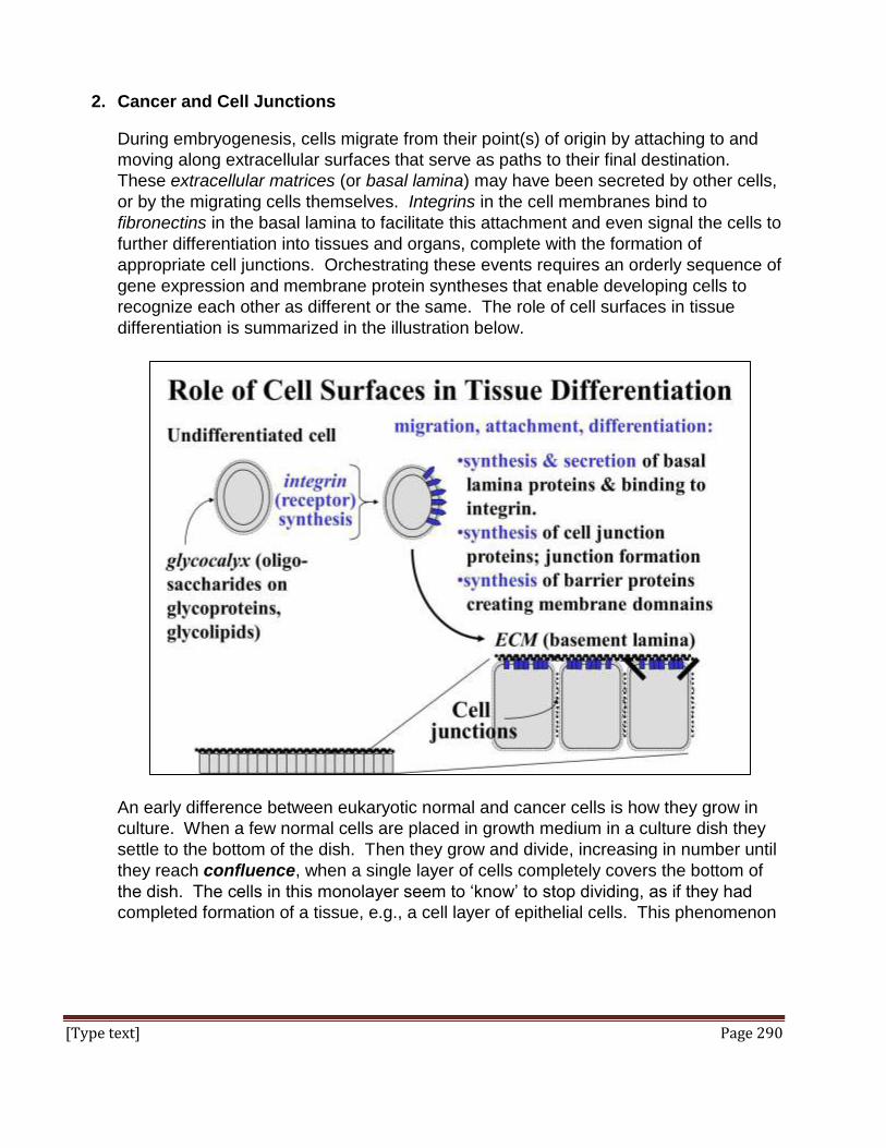
[Type text] Page 290

2. Cancer and Cell Junctions

During embryogenesis, cells migrate from their point(s) of origin by attaching to and

moving along extracellular surfaces that serve as paths to their final destination.

These extracellular matrices (or basal lamina) may have been secreted by other cells,

or by the migrating cells themselves. Integrins in the cell membranes bind to

fibronectins in the basal lamina to facilitate this attachment and even signal the cells to

further differentiation into tissues and organs, complete with the formation of

appropriate cell junctions. Orchestrating these events requires an orderly sequence of

gene expression and membrane protein syntheses that enable developing cells to

recognize each other as different or the same. The role of cell surfaces in tissue

differentiation is summarized in the illustration below.

An early difference between eukaryotic normal and cancer cells is how they grow in

culture. When a few normal cells are placed in growth medium in a culture dish they

settle to the bottom of the dish. Then they grow and divide, increasing in number until

they reach confluence, when a single layer of cells completely covers the bottom of

the dish. The cells in this monolayer seem to ‘know’ to stop dividing, as if they had

completed formation of a tissue, e.g., a cell layer of epithelial cells. This phenomenon

[Type text] Page 291

was originally called contact inhibition, implying that the cells let each other know

that they have finished forming a tissue, and that they can stop cycling and dividing.

In contrast, cancer cells do not stop dividing at confluence, but continue to grow and

divide, piling up in multiple layers. These differences in growth in culture between

normal and cancer cells are illustrated below.

Among other deficiencies in cancer cells, they do not form gap junctions and typically

have fewer cadherens and integrins in their membranes. Thus cancer cells can’t

inform each other when they reach confluence. Neither can they form firm adherens

junctions. In vivo, a paucity of integrins would inhibit cancer cells from binding and

responding to fibronectin. Therefore they also have difficulty attaching firmly to an

extracellular matrix, which may explain why many cancers metastasize, or spread

from their original site of formation.

[Type text] Page 292

VII. Signal Transduction

When hydrophobic chemical effector molecules such as steroid hormones reach a target cell

they can cross the hydrophobic membrane and bind to an intracellular receptor to initiate a

response. When large effector molecules (like protein hormones) or highly polar hormones

like adrenalin reach a target cell, they can’t cross the cell membrane. Instead they bind to

cell surfaces via transmembrane protein receptors. A conformational change initiated on the

extracellular domain of the receptor induces further allosteric change on the cytoplasmic

domain of the receptor. A series of molecular events then converts information delivered by

the external effector into intracellular information, a process called signal transduction. A

general outline of signal transduction events is illustrated below.

Many effects of signal transduction are mediated by a sequence of protein phosphorylations

catalyzed by protein kinases inside the cell. Here we consider G Protein-linked and

enzyme-linked receptors.

A. G-Protein Mediated Signal Transduction

GTP-binding proteins (G-Proteins) transduce extracellular signals by inducing production

of different second messenger molecules in the cells. When hormones or other effector

(signal) molecules bind to their membrane receptors, an allosteric change on the

cytoplasmic domain of the receptor increases the affinity of the receptor for G proteins on

the inner plasma membrane surface. G proteins are trimers consisting of , and

subunits.

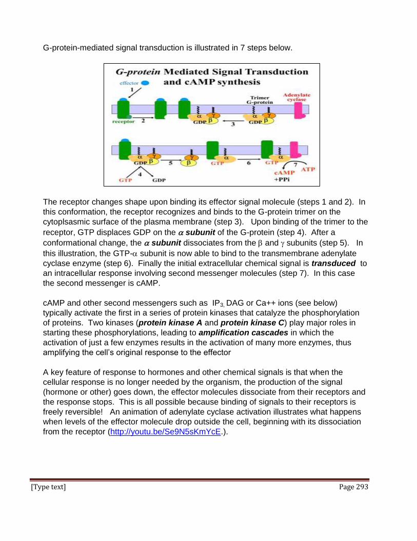
[Type text] Page 293

G-protein-mediated signal transduction is illustrated in 7 steps below.

The receptor changes shape upon binding its effector signal molecule (steps 1 and 2). In

this conformation, the receptor recognizes and binds to the G-protein trimer on the

cytoplsasmic surface of the plasma membrane (step 3). Upon binding of the trimer to the

receptor, GTP displaces GDP on the subunit of the G-protein (step 4). After a

conformational change, the subunit dissociates from the and subunits (step 5). In

this illustration, the GTP- subunit is now able to bind to the transmembrane adenylate

cyclase enzyme (step 6). Finally the initial extracellular chemical signal is transduced to

an intracellular response involving second messenger molecules (step 7). In this case

the second messenger is cAMP.

cAMP and other second messengers such as IP3, DAG or Ca++ ions (see below)

typically activate the first in a series of protein kinases that catalyze the phosphorylation

of proteins. Two kinases (protein kinase A and protein kinase C) play major roles in

starting these phosphorylations, leading to amplification cascades in which the

activation of just a few enzymes results in the activation of many more enzymes, thus

amplifying the cell’s original response to the effector

A key feature of response to hormones and other chemical signals is that when the

cellular response is no longer needed by the organism, the production of the signal

(hormone or other) goes down, the effector molecules dissociate from their receptors and

the response stops. This is all possible because binding of signals to their receptors is

freely reversible! An animation of adenylate cyclase activation illustrates what happens

when levels of the effector molecule drop outside the cell, beginning with its dissociation

from the receptor (http://youtu.be/Se9N5sKmYcE.).

[Type text] Page 294

B. Signal Transduction using PKA

Many G-protein mediated effector responses begin by activating the integral membrane

adenylate cylase. The enzyme catalyzes the hydrolysis of pyrophosphate (PPi) from

ATP and results in c-AMP synthesis. An example of a G-Protein-mediated response

involving cAMP is the fight-or-flight response to adrenaline in liver cells of higher

animals illustrated below.

After adrenalin, binds to its receptor, a G-protein mediated adenylate cyclase catalyzes

cAMP production (steps 1 an 2 in the illustration). The cAMP in the cytosol binds to two

of four subunits of an inactive enzyme protein kinase A (PKA) (step 3). A conformational

change dissociates the tetramer into two cAMP-bound inert subunits and two active PKA

subunits (step 4), each of which catalyzes phosphorylation and activation of an enzyme

called phosphorylase kinase (step 5). Phosphorylase kinase in turn catalyzes

phosphorylation of (glycogen) phosphorylase (step 6). Active glycogen phosphorylase

then catalyzes the hydrolysis glycogen to glucose-1-phosphate (step 7). This results in a

rapid retrieval free glucose from liver cells into the circulation (review glycolysis and

gluconeogenesis). Of course, the increase in circulating glucose provides energy for the

fight-or-flight decision. These events are animated at http://youtu.be/fz9Irqm0lyg.

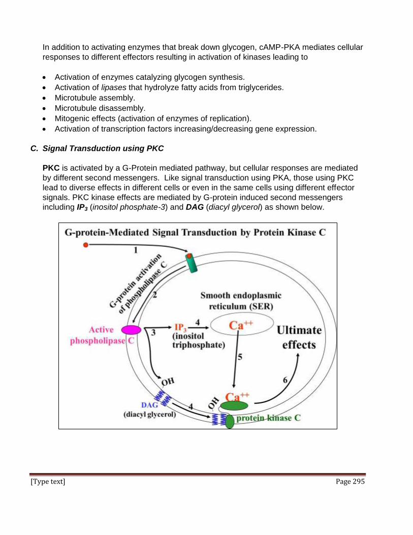
[Type text] Page 295

In addition to activating enzymes that break down glycogen, cAMP-PKA mediates cellular

responses to different effectors resulting in activation of kinases leading to

Activation of enzymes catalyzing glycogen synthesis.

Activation of lipases that hydrolyze fatty acids from triglycerides.

Microtubule assembly.

Microtubule disassembly.

Mitogenic effects (activation of enzymes of replication).

Activation of transcription factors increasing/decreasing gene expression.

C. Signal Transduction using PKC

PKC is activated by a G-Protein mediated pathway, but cellular responses are mediated

by different second messengers. Like signal transduction using PKA, those using PKC

lead to diverse effects in different cells or even in the same cells using different effector

signals. PKC kinase effects are mediated by G-protein induced second messengers

including IP3 (inositol phosphate-3) and DAG (diacyl glycerol) as shown below.

[Type text] Page 296

Like adenylate cyclase, activation of the integral membrane phospholipase C is

mediated by G proteins in response to extracellular signals (steps 1 and 2 in the

illustration). In step 3, phospholipase C action generates cytosolic inositol triphosphate

(IP3) and membrane bound diacyl glycerol (DAG). IP3 interacts with receptors on

smooth endoplasmic reticulum (step 4), causing calcium ions sequestered there to be

released into the cytoplasm (step 5). Ca++ and DAG activate Protein Kinase C (PKC).

Active PKC then initiates a phosphorylation amplification cascade leading cell-specific

responses. PKC effects include:

Neurotransmitter release.

Hormone (growth hormone, leutinizing hormone, testosterone) secretion leading to

cell growth, division and differentiation.

Glycogen hydrolysis, fat synthesis.

Additional phospholipase C effects include:

Liver glycogen breakdown.

Pancreatic amylase secretion.

Platelet aggregation

PKA and PKC are called serine-threonine kinases because the place phosphates on

serine or threonine in target polypeptides. This distinguishes their activity from the

receptor-mediated kinases discussed next.

D. Receptor Tyrosine Kinase-Mediated Signal Transduction

These combined receptor-kinases catalyze the phosphorylation of specific tyrosines in

target proteins. Furthermore, this kinase activity is in the cytoplasmic domain of the

receptor itself. Stanley Cohen and Rita Levi-Montalcini studied the effects and

mechanism of action of nerve growth factor (NGF) and epidermal growth factor

(EGF), chemical signals that stimulated growth and differentiation of nerve and skin.

Cohen’s work included the discovery of the EGF receptor, the first enzyme-linked kinase

(which was also the first tyrosine kinase) to be described.

When monomer membrane receptor kinases bind their effector ligand, they dimerize, at

which point sulfhydryl group-containing SH2 proteins) bind to each monomer, activating

the kinase domain. These initial events in receptor kinase signaling are animated at

http://youtu.be/Czs2hIWvCQQ. After multiple cross-phosphorylations of the receptor

monomers, the SH2 proteins fall away allowing the receptors to interact with other

cytoplasmic proteins in the response pathway. The basics of this complex pathway are

best viewed in the animation at http://youtu.be/FjS6HtpLOgE).

[Type text] Page 297

Many so-called cancer genes, or oncogenes, are really mutations of genes involved in

normal growth and differentiation. Some of these are in mitogenic signal transduction

pathways. Under normal circumstances, mitogenic chemical signals (like EGF) bind to

their receptors and induce target cells to begin dividing. Mutations in genes for proteins in

these signal transduction pathways (a well-studied example is animated at

http://youtu.be/m9cVMHFKDhY) can leave them active even in the absence of timely

signaling, resulting in uncontrolled (cancerous) cell division. MAP (mitogen-activated

protein) kinase is a central protein in receptor kinase signaling pathways. This enzyme

can phosphorylate inactive transcription factors and other nuclear proteins that affect

gene activity leading to cell proliferation and differentiation, as illustrated below.

E. Signal Transduction in Evolution

We have seen that signal transduction characteristically takes a few signal molecules interacting with cell surface receptors and amplifies a response in a cascade of enzymatic reactions in which proteins are phosphorylated to activate them (or in some cases, inactivate them). Amplification cascades can take a single effector-receptor interaction and magnify its effect in the cell by orders of magnitude, making the signaling systems highly efficient. The range of cellular and systemic (organismic) responses to the same chemical signal is broad and complex since different cell types can have receptors for the

[Type text] Page 298

same effector, but will respond differently. Thus, adrenaline is a hormone that targets liver cells and blood vessels among others, with different effects in each cell type. And, adrenaline is also a neurotransmitter. What seems to have happened in evolution is that as organisms became more complex in response to environmental imperatives, they have adapted by co-opting already existing signaling systems in the service of new pathways.

Just as the same signal transduction event can lead to different pathways of response in different cells, evolution has allowed different signal transduction pathways to engage in crosstalk. This is when two different signal transduction pathways intersect in the same cells. In one example, the cAMP produced at the front end of the PKA signaling pathway can activate (or under the right circumstances, inhibit) enzymes in the MAP kinase pathway. These effects result in changes in the levels of active or inactive transcription factors and therefore a modulation of gene expression by two (or more) signals. We are only beginning to understand what looks more like a web of signal transduction and less like a linear pathway.

Some iText & VOP Key Words and Terms

action potential fight-or-flight peroxisomes

active transport flaccid phagocytosis

adaptin free energy phospholipase C

adenylate cyclase G protein subunits phosphorylase kinase

adherens junctions gap junctions pinocytosis

adrenaline gluconeogenesis PKA

allosteric change regulates transport

GLUT1 PKC

antiport glycolysis plasmodesmata

aquaporins good cholesterol plasmolysis

bad cholesterol G-Protein-linked receptors poikilothermic organisms

basal lamina Heat shock protein potential difference

belt desmosomes HSP70 protein Protein kinase A

Ca++ ions hydrophilic corridor protein kinase C

cadherin hypertonic protein packaging

cargo receptor hypotonic protein phosphorylation

carrier proteins IgG light chain proton gate

cell adhesion molecules inositol triphosphate proton pump

cell-cell attachment integrin receptor-mediated endocytosis

cell-cell recognition ion channels RER membrane

cell-free translation ion flow resting potential

[Type text] Page 299

channel proteins ion pumps secondary active transporters

chaperone proteins IP3 serine-threonine kinases

cholesterol effects in membranes

isotonic signal peptide

clathrin LDL (low density lipoprotein)

signal recognition particle

coated pits ligand (chemically) gated channels

signal sequence

coated vesicle lysosome signal transduction

connexins MAP kinase Smooth endoplasmic reticulum

contact inhibition mechanically gated channels

sodium-potassium pump

contractile vacuole membrane depolarization solute concentration gradients

COP membrane hyperpolarization

solute transport

cotransport membrane invagination sorting vesicle

coupled transport membrane potential spot desmosomes

cytoskeleton microbodies stop-transfer sequence

DAG mitochondrial membane contact proteins

symport

diffusion kinetics mitogenic effects tight junction membrane proteins

early endosome nerve growth factor tight junctions

ECM neurotransmitters TJMPs

effector molecules NGF tonoplast

EGF nuclear envelope T-SNARE

endocytosis nuclear pore fibrils turgid

endomembrane system nuclear transport receptor turgor pressure

Enzyme-lined receptors O-glycosylation tyrsine kinases

epidermal growth factor osmoregulation uniport

excitability osmosis uphill v. downhill solute movement

exocytosis osmotic pressure voltage gated channels

facilitated diffusion passive diffusion V-SNARE

fibronectin patch clamp techniques

[Type text] Page 300

Chapter 15: The Cytoskeleton & Cell Motility

Microfilaments, intermediate filaments and microtubules – roles in cell structure,

secretion, cell migration and other organelle movements

I. Overview of the Cytoskeleton

The cell as it appears in a microscope was long thought to be a bag of liquid surrounded by a membrane. The electron microscope revealed a cytoskeleton composed of tubes, rods and filaments in witch other intracellular structures were enmeshed. We will compare the molecular compositions of these structures and their subunit proteins. The cytoskeleton accounts for the location of organelles in cells and the shapes of cells themselves. We’ll see how cytoskeletal components also account for cell motility, which includes how cells and organisms move as well as how structures within cells (often vesicles) move from one part of the cell to another. These movements are not random! A long- and well-studied system of cell motility is the interaction of actin and myosin during skeletal muscle contraction. We will first consider a paradox which suggested that ATP was required for contraction AND for relaxation of muscle fibers. Then we look at experiments resolving the paradox. Some muscles in the animal body contract rhythmically with little or no control on the part of the animal (think heart). But animals do control when they contract their skeletal muscles, implying that this kind of contraction is regulated. We will take a look at the role calcium ions and the regulatory proteins that control skeletal muscle contraction. Voice-Over PowerPoint Presentations The Cytoskeleton – Microtubules, Microfilaments and Intermediate Filaments VOP The Actin-Myosin Contraction Paradox VOP Resolving the Actin-Myosin Contraction Paradox VOP Regulation of Skeletal Muscle Contraction VOP Learning Objectives

When you have mastered the information in this chapter and the associated VOPs, you

should be able to:

1. compare and contrast the roles of microfilaments and microtubules in different forms of cell motility.

2. distinguish the roles of microfilaments, microtubules and intermediate filaments in the maintenance and alteration of cell shape and structure.

3. state an hypothesis explaining how microtubules in cilia maintain their length. 4. propose an experiment to determine which part of a motor protein has the ATPase

activity. 5. define the actin-myosin, or contraction paradox.

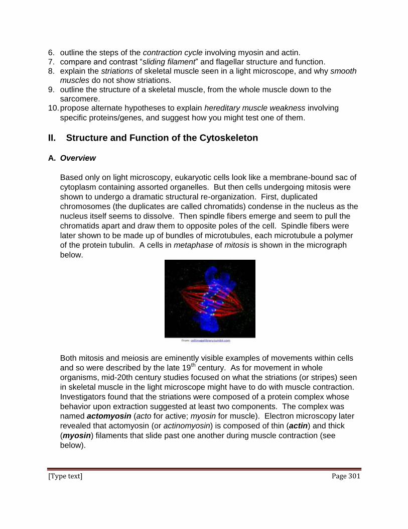
[Type text] Page 301

6. outline the steps of the contraction cycle involving myosin and actin. 7. compare and contrast “sliding filament” and flagellar structure and function. 8. explain the striations of skeletal muscle seen in a light microscope, and why smooth

muscles do not show striations. 9. outline the structure of a skeletal muscle, from the whole muscle down to the

sarcomere. 10. propose alternate hypotheses to explain hereditary muscle weakness involving

specific proteins/genes, and suggest how you might test one of them.

II. Structure and Function of the Cytoskeleton

A. Overview

Based only on light microscopy, eukaryotic cells look like a membrane-bound sac of

cytoplasm containing assorted organelles. But then cells undergoing mitosis were

shown to undergo a dramatic structural re-organization. First, duplicated

chromosomes (the duplicates are called chromatids) condense in the nucleus as the

nucleus itself seems to dissolve. Then spindle fibers emerge and seem to pull the

chromatids apart and draw them to opposite poles of the cell. Spindle fibers were

later shown to be made up of bundles of microtubules, each microtubule a polymer

of the protein tubulin. A cells in metaphase of mitosis is shown in the micrograph

below.

Both mitosis and meiosis are eminently visible examples of movements within cells

and so were described by the late 19th century. As for movement in whole

organisms, mid-20th century studies focused on what the striations (or stripes) seen

in skeletal muscle in the light microscope might have to do with muscle contraction.

Investigators found that the striations were composed of a protein complex whose

behavior upon extraction suggested at least two components. The complex was

named actomyosin (acto for active; myosin for muscle). Electron microscopy later

revealed that actomyosin (or actinomyosin) is composed of thin (actin) and thick

(myosin) filaments that slide past one another during muscle contraction (see

below).

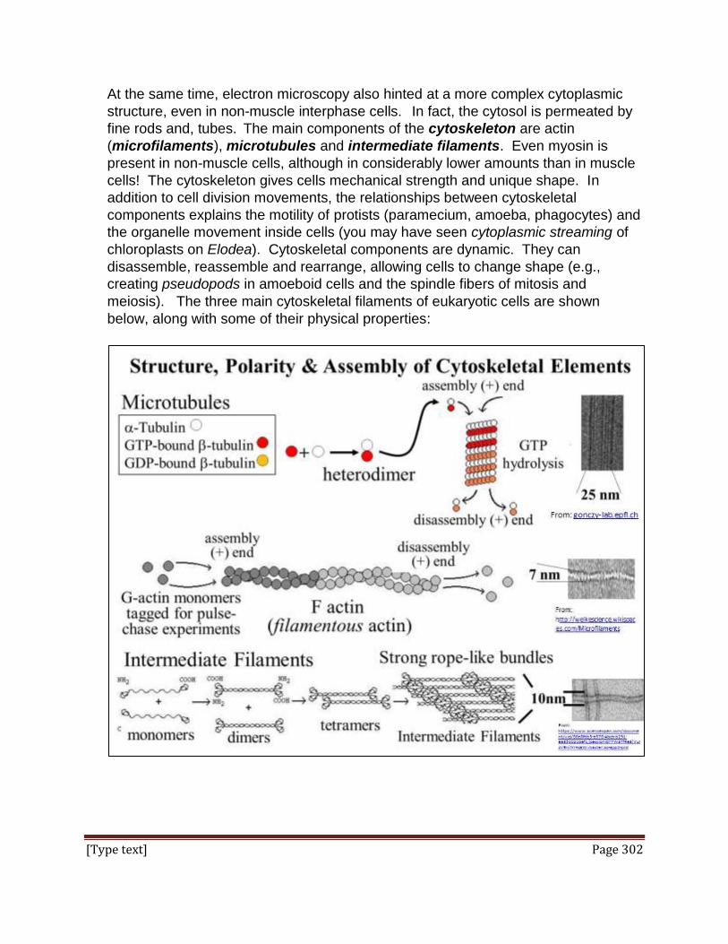
[Type text] Page 302

At the same time, electron microscopy also hinted at a more complex cytoplasmic

structure, even in non-muscle interphase cells. In fact, the cytosol is permeated by

fine rods and, tubes. The main components of the cytoskeleton are actin

(microfilaments), microtubules and intermediate filaments. Even myosin is

present in non-muscle cells, although in considerably lower amounts than in muscle

cells! The cytoskeleton gives cells mechanical strength and unique shape. In

addition to cell division movements, the relationships between cytoskeletal

components explains the motility of protists (paramecium, amoeba, phagocytes) and

the organelle movement inside cells (you may have seen cytoplasmic streaming of

chloroplasts on Elodea). Cytoskeletal components are dynamic. They can

disassemble, reassemble and rearrange, allowing cells to change shape (e.g.,

creating pseudopods in amoeboid cells and the spindle fibers of mitosis and

meiosis). The three main cytoskeletal filaments of eukaryotic cells are shown

below, along with some of their physical properties:

[Type text] Page 303

While intermediate filaments serve a mainly structural role in cells, microtubules and

microfilaments have dual functions, both in maintaining and changing cell shape

and in enabling cell motility. For example, by attaching to components of the plasma

membrane, microfilaments contribute to maintain cell shape, but by interacting

with motor proteins in cells (e.g., myosin), they can move against the membrane

causing changes in cell shape. Likewise, motor proteins such as dynein and kinesin

proteins along microtubule tracks to bring ‘cargo’ from one point to another in the

cell. The general location of different cytoskeletal components is shown in the

illustration and micrographs of typical animal cells below:

These localizations hint at (or are consistent with known) functions of microtubules,

microfilaments and intermediate filaments in cell structure and motility.

[Type text] Page 304

More recently, elements of a cytoskeleton have been demonstrated in prokaryotic

cells - thus all cells are more than a bag of sap with no particular organization! Next,

we’ll consider the role of microtubules, microfilaments, intermediate filaments and

related proteins in the cytoskeleton.

B. Microtubules – an Overview

Microtubules assemble from and tubulin monomers. After forming tubulin

dimers, the dimers add to a growing plus, or +end. Assembly is fueled by GTP

hydrolysis. Dynamic microtubules involved in changing the shape of cells or in

spindle fibers during mitosis or meiosis will disassemble at the opposite minus, or -

end.

Individual microtubules can be isolated. These ‘purified’ microtubules were shown to

grow by addition to one end and to disassemble at the opposite end, thereby

demonstrating +ends and –ends. A summary of the experiment that demonstrated

this ‘polarity’ of microtubules is animated at http://youtu.be/CkeYBSD9RJg

Microtubules in cells can seem disordered, although they tend to radiate from

centrioles in non-dividing animal cells. In dividing cells, we say that microtubule

formation is nucleated from centrioles in animal cells and from a more amorphous

microtubule organizing center (MTOC) plant cells. A typical centriole (or basal

body) in cross section has a ‘9 triplet’ microtubule array as seen below.

1. The Two kinds of Microtubules in Spindle Fibers

Kinetochore microtubules

At prophase of mitosis and meiosis, duplicated chromosomes condense,

becoming visible as paired chromatids attached at their centromeres.

During condensation, proteins associate with the centromeres of the

chromatids to create a kinetochore. As the spindle apparatus forms, some

[Type text] Page 305

spindle fibers attach to the kinetochore. By metaphase these spindles

(bundles of microtubules) are seen stretching from kinetochores at the center

of the cell to the centrioles or MTOCs of the dividing cells.

We now know that the assembly or growth ends (+ends) of kinetochore

microtubules are at the kinetochore! At anaphase, chromatids are separated

by forces generated when microtubules shorten at their disassembly ends

(their –ends) at the centrioles/MTOC. Microtubule disassembly also provides

the force that draws daughter chromosomes to the opposite poles of the cell

as cell division continues.

Polar microtubules

These microtubules extend from centrioles/MTOCs at the poles, overlapping

at the center of dividing cells. These microtubules slide past one another in

opposite directions during anaphase. The effect is to push apart the poles of

the cell., even as the chromatids are being pulled to the opposite poles. But

in this case, ATP hydrolysis powers a motor protein called dynein attached

to one microtubule that in effect ‘walks’ along a microtubule extending from

the opposite pole of the cell.

The roles of polar and kinetochore microtubules are illustrated in below.

The role of microtubule disassembly at the centrioles (i.e., the minus end)

was demonstrated in a clever experiment in which a tiny laser beam was

aimed into a cell at spindle fibers attached to the kinetochore of a pair of

chromatids. What happened when the laser cut the spindle fiber is animated

at http://youtu.be/1PSenpp7TmE.

[Type text] Page 306

2. Microtubules in Cilia and Flagella

The microtubules of cilia or flagella emerge from a basal body (below left).

Basal bodies are structurally similar to centrioles, organized as a ring of 9

triplets. Cilia and flagella formation begin at basal bodies but show a typical

9+2 (nine outer doublet plus two central) microtubule arrangement in cross

section. When cilia or flagella are isolated and their membranes are

removed, what remains is the axoneme, which preserved the 9+2 microtubule

arrangement. Isolated axonemes can be seen with no surrounding

membrane (below right).

The structural relationship between the axoneme of a cilium or flagellum and

an individual microtubule is shown below.

[Type text] Page 307

In cross section it is possible to see the tubulin subunits that make up a

microtubule polymer. Each tubule is made up of a ring of 13 tubulin subunits.

The microtubules in the ‘doublets’ share tubulins, but are also composed of

13 tubulins. When fully formed, the 25 nm diameter microtubules appear to

be a hollow cylinder. But microtubules are typically isolated with motor

proteins and other Microtubule-Associated Proteins (MAPs).

3. Microtubule Motor Proteins Move Cargo from Place to Place in Cells

Motor proteins are ATPases that use the free energy of ATP hydrolysis to

power cellular and intracellular motility. Let’s take a closer look at how two

major motor proteins, dynein and kinesin, carry cargo from place to place

inside of cells. Organelles are a typical cargo. Examples include moving

secretory vesicles trans Golgi vesicles to the plasma membrane for

exocytosis. Vesicles containing neurotransmitters also move along

microtubule tracks running from the cell body to the nerve ending. And in a

chameleon moving between light and dark background foliage, pigment

vesicles in skin cells disperse or aggregate along microtubule tracks to

change skin color to match the background. The role of kinesin and dynein

motor proteins in carrying neurotransmitter vesicles in opposite directions

along axonal microtubules is well understood. Kinesin moves

neurotransmitter vesicles (e.g., protein neurotransmitters made in the

endomembrane system) to nerve endings (anterograde movement). In

contrast, as part of a dynactin complex, dynein moves empty vesicles back

to the cell body (retrograde movement). This is illustrated below, along with

some details of motor protein structure.

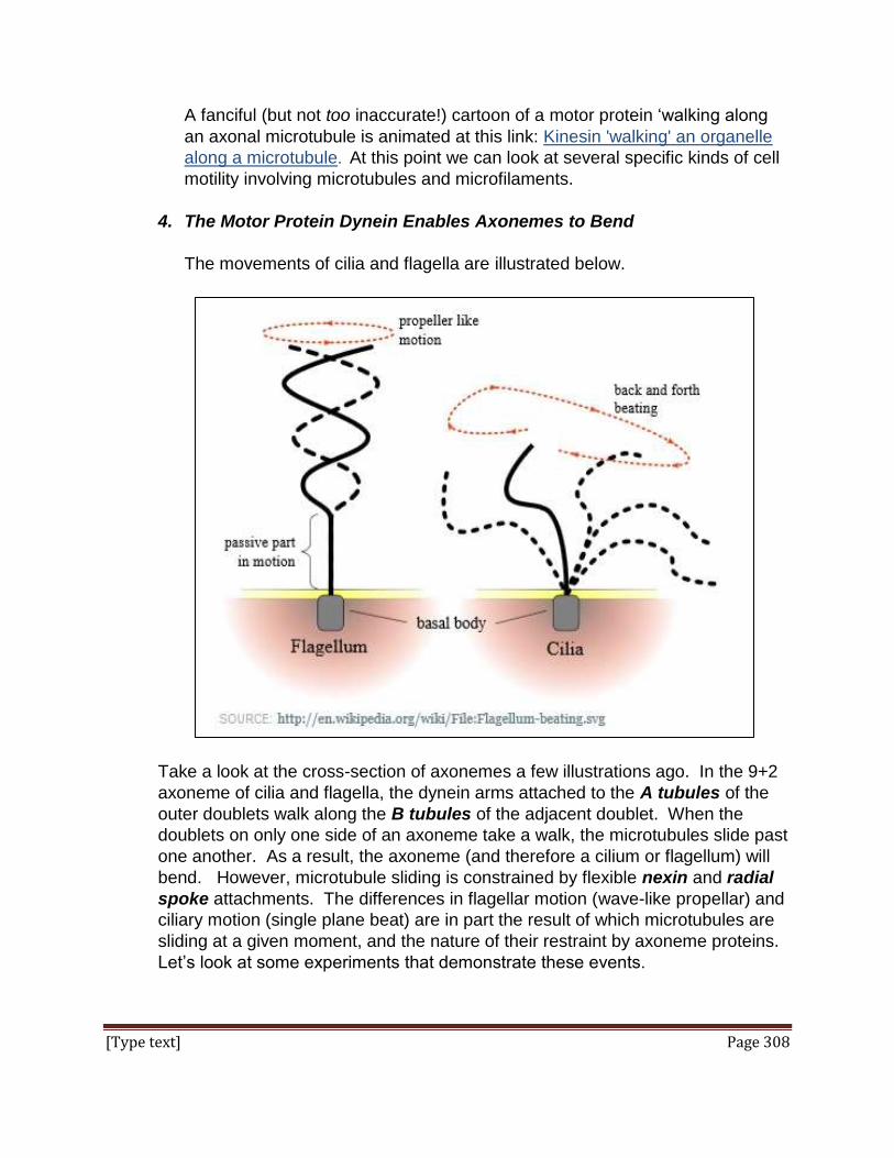
[Type text] Page 308

A fanciful (but not too inaccurate!) cartoon of a motor protein ‘walking along

an axonal microtubule is animated at this link: Kinesin 'walking' an organelle

along a microtubule. At this point we can look at several specific kinds of cell

motility involving microtubules and microfilaments.

4. The Motor Protein Dynein Enables Axonemes to Bend

The movements of cilia and flagella are illustrated below.

Take a look at the cross-section of axonemes a few illustrations ago. In the 9+2

axoneme of cilia and flagella, the dynein arms attached to the A tubules of the

outer doublets walk along the B tubules of the adjacent doublet. When the

doublets on only one side of an axoneme take a walk, the microtubules slide past

one another. As a result, the axoneme (and therefore a cilium or flagellum) will

bend. However, microtubule sliding is constrained by flexible nexin and radial

spoke attachments. The differences in flagellar motion (wave-like propellar) and

ciliary motion (single plane beat) are in part the result of which microtubules are

sliding at a given moment, and the nature of their restraint by axoneme proteins.

Let’s look at some experiments that demonstrate these events.

[Type text] Page 309

The sliding microtubule mechanism of ciliary and flagellar motility was

determined by experiments on isolated axonemes. One such experiment is

illustrated below.

Agitating sperm or ciliated cells in a high speed blender for a few seconds will shear and detach flagella or cilia from the rest of the cell. Adding ATP to either will cause them to beat, a phenomenon easily seen in a light microscope. Axonemes isolated from detached cilia or flagella by detergent treatment (to disrupt membranes) retain their characteristic 9+2 microtubule arrangement as well as other ultrastructural features. And even isolated axonemes will beat in the presence of ATP!

[Type text] Page 310

Additional detergent treatment removes radial spokes, nexin and other proteins from the axoneme, causing the microtubules to separate. Dissociated microtubule doublets and central ‘singlets’ could be observed in the electron microscope. When such separated microtubules are dialyzed to remove the detergents, the doublet microtubules re-associate, forming sheets, as shown in the cartoon below.

When ATP is added back to the ‘reconstituted’ microtubule doublets, they again separate as the ATP is hydrolyzed. And if such preparations are fixed for electron microscopy immediately after adding the ATP, they can be caught in the act of sliding! The interpretation of these electron microscope observations is at http://youtu.be/Y6RBJfUpZec.

C. Microfilaments – an Overview

At 7 nm in diameter, microfilaments (actin filaments) are the thinnest component of

the cytoskeleton. Globular actin protein monomers (G-actin) polymerize to form a

linear F-actin polymer. Two polymers combine to form the twin helical actin

microfilament. As with microtubules, microfilaments have a +end to which new actin

monomers are added to assemble the F-actin and a –end at which the

microfilaments disassemble when they are in a dynamic state, such as when a cell is

changing shape. When one end of a microfilament is anchored to a cellular

structure, for example to plaques in the cell membrane, motor proteins (e.g.,

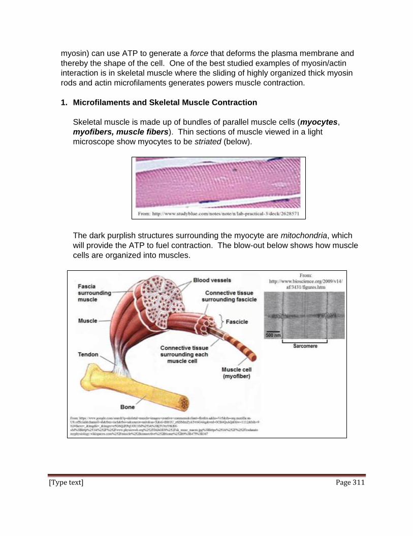
[Type text] Page 311

myosin) can use ATP to generate a force that deforms the plasma membrane and

thereby the shape of the cell. One of the best studied examples of myosin/actin

interaction is in skeletal muscle where the sliding of highly organized thick myosin

rods and actin microfilaments generates powers muscle contraction.

1. Microfilaments and Skeletal Muscle Contraction

Skeletal muscle is made up of bundles of parallel muscle cells (myocytes,

myofibers, muscle fibers). Thin sections of muscle viewed in a light

microscope show myocytes to be striated (below).

The dark purplish structures surrounding the myocyte are mitochondria, which

will provide the ATP to fuel contraction. The blow-out below shows how muscle

cells are organized into muscles.

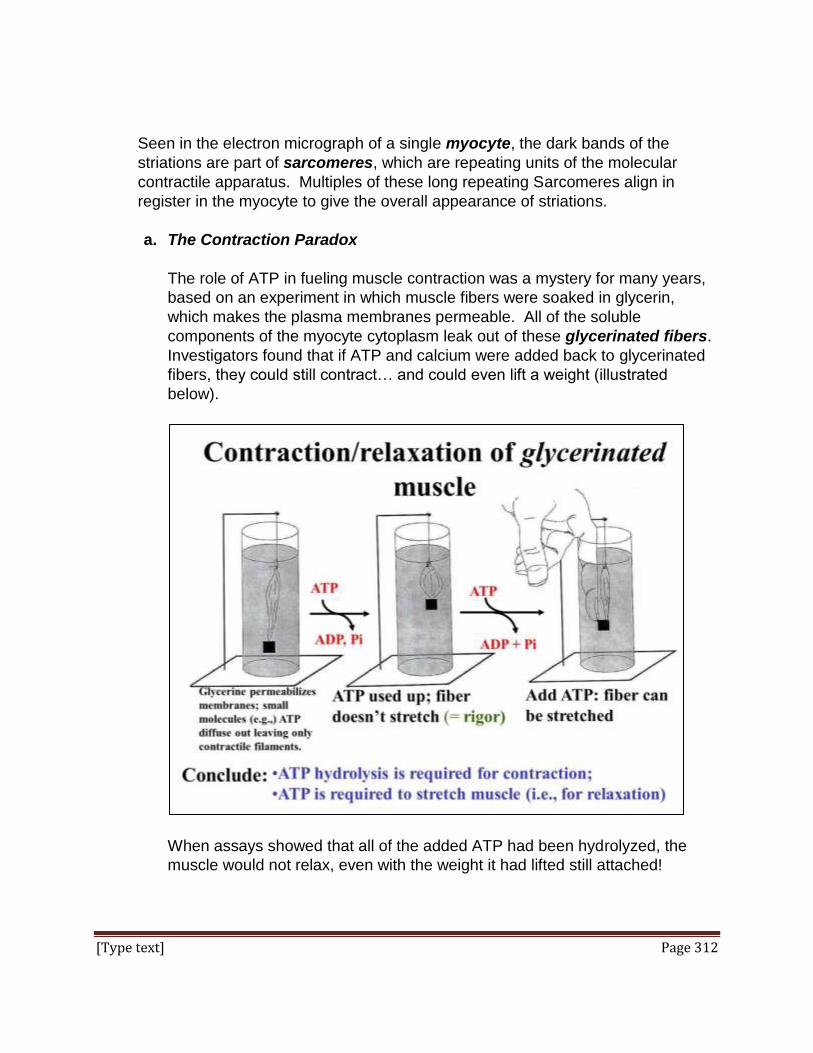
[Type text] Page 312

Seen in the electron micrograph of a single myocyte, the dark bands of the

striations are part of sarcomeres, which are repeating units of the molecular

contractile apparatus. Multiples of these long repeating Sarcomeres align in

register in the myocyte to give the overall appearance of striations.

a. The Contraction Paradox

The role of ATP in fueling muscle contraction was a mystery for many years,

based on an experiment in which muscle fibers were soaked in glycerin,

which makes the plasma membranes permeable. All of the soluble

components of the myocyte cytoplasm leak out of these glycerinated fibers.

Investigators found that if ATP and calcium were added back to glycerinated

fibers, they could still contract… and could even lift a weight (illustrated

below).

When assays showed that all of the added ATP had been hydrolyzed, the

muscle would not relax, even with the weight it had lifted still attached!

[Type text] Page 313

Attempting to manually force the muscle back to its relaxed position didn’t

work. But if fresh ATP was added to the preparation, it was possible to

stretch the fiber. And if after stretching the fiber the experimenter let go, the

muscle would again contract and lift the weight. A cycle of forced stretching

and contraction could be repeated until all of the ATP was hydrolyzed, at

which point the fiber could no longer contract or could no longer be stretched.

The contraction paradox then, was that ATP hydrolysis was required for

muscle contraction as well as for relaxation (stretching). The paradox was

resolved when the functions of the molecular actors of contraction were finally

understood. Here we review some of the classic experiments that led to this

understanding.

b. Actomyosin and the Sliding Filament Model of Skeletal Muscle

Contraction

Early extractions of homogenates of skeletal muscle led to the isolation of a

viscous substance named actomyosin (acto for active and myosin for muscle

substance). Under the right conditions, adding ATP to actomyosin

preparations caused a decrease in viscosity, but after a while (i.e., after the

added ATP was hydrolyzed), the mixture became viscous again. Further

extraction of the non-viscous preparation (before it re-congealed) led to the

separation of two main substances, actin and myosin. Adding these

components back together reconstituted the viscous actomyosin extract (now

often referred to as actinomyosin to reflect its composition).

High resolution electron microscopy in the 19040s revealed the fine structure

of skeletal muscle, allowing characterization of the sarcomere (below).

[Type text] Page 314

In this micrograph of a sarcomere from relaxed muscle, two Z-lines

demarcate the sarcomere (Z for zwischen, German for ‘between’). Thin

(actin) filaments can be seen coming from the Z lines towards the myosin

filaments which are thicker than the actin microfilaments. The region of the

actin filaments are the I bands while the region of the thick myosin filaments

makes up the A band, with an M line running down its center. The H zone

includes the M line and the lighter region on either side of the M line. Electron

micrographs of sarcomeres from relaxed and contracted skeletal muscle are

shown below.

The micrographs show that the H zone has almost disappeared in the

sarcomere of the contracted muscle cell. While the width of the A band has

not changed, those of the I bands have decreased and the Z-lines are closer

together after contraction. Given that the thin filaments are part of the I bands

and the A band is composed mainly of thick filaments, the suggestion was

that during contraction, the thin filaments slide along the thick filaments,

drawing the Z-lines (to which they are attached) closer together. This was

called the sliding filament hypothesis, or model of skeletal muscle

contraction.

[Type text] Page 315

The sliding filament model is diagrammed below.

c. Actin-Myosin Interactions in Contraction

Recall the early purification of actomyosin components from skeletal muscle

cells (above). After adding ATP, the separated components were examined

in the electron microscope. Both thick (myosin) and thin (actin) filaments

were recognized as separate entities that could be separated by

centrifugation (as cartooned below).

In these experiments, actin filaments were still attached to Z-lines.

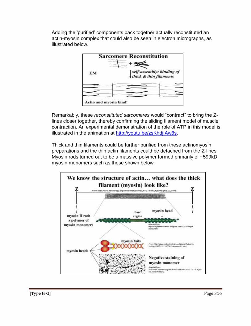
[Type text] Page 316

Adding the ‘purified’ components back together actually reconstituted an

actin-myosin complex that could also be seen in electron micrographs, as

illustrated below.

Remarkably, these reconstituted sarcomeres would “contract” to bring the Z-

lines closer together, thereby confirming the sliding filament model of muscle

contraction. An experimental demonstration of the role of ATP in this model is

illustrated in the animation at http://youtu.be/zsKhdjIAw8s.

Thick and thin filaments could be further purified from these actinomyosin

preparations and the thin actin filaments could be detached from the Z-lines.

Myosin rods turned out to be a massive polymer formed primarily of ~599kD

myosin monomers such as those shown below.

[Type text] Page 317

An early observation was isolated actin filaments had no ATPase activity. But

while myosin preparations did have an ATPase activity, they would only

catalyze ATP hydrolysis very slowly compared to muscle fibers. Faster ATP

hydrolysis occurred only if the myosin filaments were mixed with

microfilaments (on or off Z-lines).

In the electron microscope, isolated myosin protein monomers appeared to

have head and tail regions. The monomers were shown to be composed of a

pair of heavy chain and two pairs of light chain polypeptides (below).

Treatment of monomers with certain proteolytic enzymes that hydrolyze

peptide linkages only between specific amino acids was shown to ‘break’

peptide linkages within the heavy chains. The resulting S1 and tail fragments

could be separated by ultracentrifugation, examined in the electron

microscope and assayed for ATPase activity. It turned out that the S1

fraction of myosin heads had a slow ATPase activity while the tails had none.

The slow activity was not an artifact of isolation since if the S1 fraction was

mixed with action filaments, the catalytic rate increased. The S1 fragments

were then shown to also contain an action-binding domain.

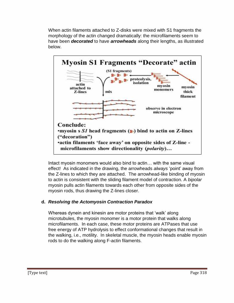
[Type text] Page 318

When actin filaments attached to Z-disks were mixed with S1 fragments the

morphology of the actin changed dramatically: the microfilaments seem to

have been decorated to have arrowheads along their lengths, as illustrated

below.

Intact myosin monomers would also bind to actin… with the same visual

effect! As indicated in the drawing, the arrowheads always ‘point’ away from

the Z-lines to which they are attached. The arrowhead-like binding of myosin

to actin is consistent with the sliding filament model of contraction. A bipolar

myosin pulls actin filaments towards each other from opposite sides of the

myosin rods, thus drawing the Z-lines closer.

d. Resolving the Actomyosin Contraction Paradox

Whereas dynein and kinesin are motor proteins that ‘walk’ along

microtubules, the myosin monomer is a motor protein that walks along

microfilaments. In each case, these motor proteins are ATPases that use

free energy of ATP hydrolysis to effect conformational changes that result in

the walking, i.e., motility. In skeletal muscle, the myosin heads enable myosin

rods to do the walking along F-actin filaments.

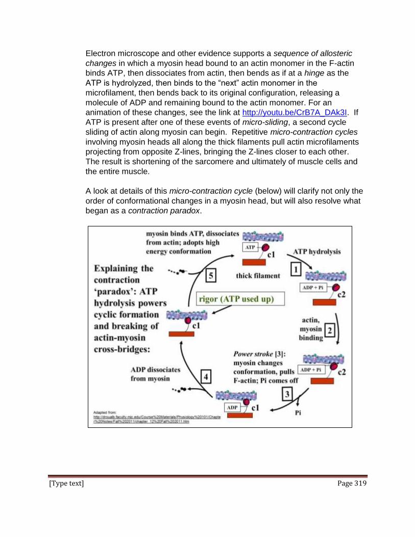
[Type text] Page 319

Electron microscope and other evidence supports a sequence of allosteric

changes in which a myosin head bound to an actin monomer in the F-actin

binds ATP, then dissociates from actin, then bends as if at a hinge as the

ATP is hydrolyzed, then binds to the “next” actin monomer in the

microfilament, then bends back to its original configuration, releasing a

molecule of ADP and remaining bound to the actin monomer. For an

animation of these changes, see the link at http://youtu.be/CrB7A_DAk3I. If

ATP is present after one of these events of micro-sliding, a second cycle

sliding of actin along myosin can begin. Repetitive micro-contraction cycles

involving myosin heads all along the thick filaments pull actin microfilaments

projecting from opposite Z-lines, bringing the Z-lines closer to each other.

The result is shortening of the sarcomere and ultimately of muscle cells and

the entire muscle.

A look at details of this micro-contraction cycle (below) will clarify not only the

order of conformational changes in a myosin head, but will also resolve what

began as a contraction paradox.

[Type text] Page 320

The myosin head micro-contraction cycle resolves the contraction paradox

as follows:

ATP is necessary for muscle contraction: When ATP is hydrolyzed

myosin heads undergo a transition from a low energy conformation

(c1) to a high energy conformation (step [1]). In this conformation, the

myosin heads bind to actin monomers in the microfilament (step [2]).

This binding results the power stroke (step [3]) in which ATP

hydrolysis and a allosteric change in myosin (back to the c1

conformation) that pulls the actin along the myosin. in effect causing a

micro-shortening of the sarcomere. Pi bound to the head after ATP

hydrolysis is released during the power stroke.

ATP (but not its hydrolysis!) is necessary for muscle relaxation: In

step [4], the ADP still bound to the myosin head is released. In this

state, the myosin head will remain bound to actin until ATP can again

bind to the myosin head (step [5[), causing dissociation of myosin from

actin, and starting the micro-contraction cycle again.

In the absence of ATP (as after the death of an organism), the micro-

contraction cycle is interrupted as all myosin heads remain bound to the

actin filaments in whatever the state of muscle contraction or relaxation

(stretch) was at the time of death. This is rigor mortis at the molecular

level. At the level of whole muscle, rigor mortis is seen in an inability to

stretch or otherwise move body parts.

e. Regulating Skeletal Muscle Contraction

An action potential at a neuromuscular junction initiates contraction:

[Type text] Page 321

Typically, acetylcholine released by a motor neuron binds to receptors on

muscle cells to initiate contraction. In early experiments, Ca++ was shown

to be needed along with ATP to get glycerinated skeletal muscle to

contract. It was subsequently demonstrated that Ca++ ions were stored in

the smooth endoplasmic reticulum of muscle cells (or sarcoplasmic

reticulum). As we have already seen, an action potential generated in

the cell body of a neuron can be propagated along an axon to the nerve

terminal, or synapse. In a similar fashion, an action potential generated at

a neuromuscular junction travels along the sarcolemma to points where

the sarcolemma is continuous with transverse tubules (T-tubules). The

action potential then moves along the T-tubules and then along the

sarcoplasmic reticulum. This propagation of an action potential opens

Ca++ channels in the sarcoplasmic reticulum. The Ca++ released bathes

the sarcomeres of the myofibrils, allowing filaments to slide (i.e.,

contraction). This process is shown above and animated at this link:

http://youtu.be/HpZpA-vYDBU.

The molecular basis of Ca++ ion regulation of muscle contraction involves

4 proteins that are bound to actin microfilaments in skeletal muscle.

These proteins (three troponin subunits and tropomyosin) are shown

lying on actin in the illustration below.

[Type text] Page 322

Ca++ ions bind to troponins along the actin filaments causing

conformational changes in troponins and tropomyosin that expose myosin-

binding sites on actin. Only then can ATP-bound myosin bind to actin and

initiate the micro-contraction cycle illustrated earlier. The allosteric

changes initiated by Ca++ binding are shown in greater detail in the

drawing of an actin filament in cross-section, below.

In resting muscle, tropomyosin (a fibrous protein) lies along the actin

filament, covering up the myosin binding sites on seven G-actin subunits

in the filament. In this conformation, troponin T (tropomyosin-binding

troponin) and troponin I (inhibitory troponin) hold the tropomyosin in

place. A chain reaction of conformational changes begins when Ca++

ions bind to troponin-C (Ca++-binding troponin). The result is that

tropomyosin shifts position along the filament to expose the myosin-

binding sites on the G-actin subunits.

2. Muscle contraction generates force

Contraction by ATP-powered sliding of thin along thick filaments generates force

on the Z-lines (in 3 dimensions, these are actually Z-disks) to which the actin

thin filaments are attached. The protein -actinin in the Z-disks anchors the

ends of the actin filaments to the disks so that when the filaments slide, the Z-

disks are drawn closer, shortening the sarcomeres. Another Z-disk protein,

desmin, is an intermediate filament organized around the periphery of Z-disks.

Desmin connects multiple Z-disks in a myofibril. By keeping the Z-Disks in

register, muscle cell, and ultimately, muscle contraction is coordinated.

[Type text] Page 323

Finally, for a muscle cell to shorten during contraction of myofibrils, the actin

filaments at the ends of the cell must be connected to the cell membrane. Several

proteins, including syntrophins and dystrophin (another intermediate filament

protein) anchor the free ends of microfilaments coming from Z-disks to the cell

membrane. Still other proteins anchor the cell membrane in this region to the

extracellular matrix (tendons) that are attached to bones! Force generated by

myosin hydrolysis of ATP and the sliding of filaments in individual sarcomeres is

thus transmitted to the ends of muscles to effect movement. If the name

dystrophin sounds familiar, it should! The protein is named for a mutation that

causes muscular dystrophy, characterized by progressive weakening of the

muscles. Like many genes, the dystrophin gene gets its name from the

malfunctions caused by its mutation.

3. Non-muscle Microfilaments

Electron microscopy revealed thin filaments in the cytoskeleton of eukaryotic

cells. When myosin S1 heads placed atop electron micrograph thin sections

were shown to decorate these microfilaments with arrowheads, it was clear that

they were a form of F-actin. Decorated actin in the microfilament bundles of

microvilli in the brush border of epithelial cells are shown below.

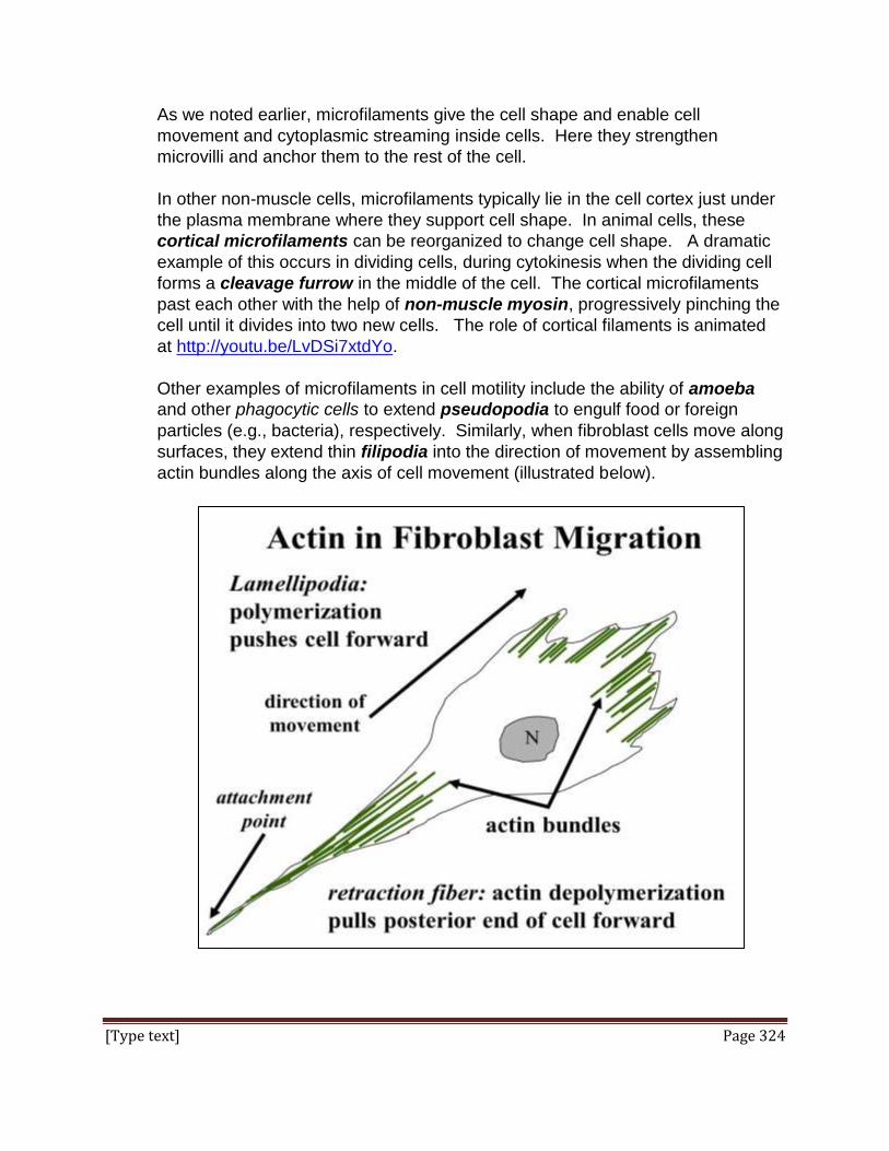
[Type text] Page 324

As we noted earlier, microfilaments give the cell shape and enable cell

movement and cytoplasmic streaming inside cells. Here they strengthen

microvilli and anchor them to the rest of the cell.

In other non-muscle cells, microfilaments typically lie in the cell cortex just under

the plasma membrane where they support cell shape. In animal cells, these

cortical microfilaments can be reorganized to change cell shape. A dramatic

example of this occurs in dividing cells, during cytokinesis when the dividing cell

forms a cleavage furrow in the middle of the cell. The cortical microfilaments

past each other with the help of non-muscle myosin, progressively pinching the

cell until it divides into two new cells. The role of cortical filaments is animated

at http://youtu.be/LvDSi7xtdYo.

Other examples of microfilaments in cell motility include the ability of amoeba

and other phagocytic cells to extend pseudopodia to engulf food or foreign

particles (e.g., bacteria), respectively. Similarly, when fibroblast cells move along

surfaces, they extend thin filipodia into the direction of movement by assembling

actin bundles along the axis of cell movement (illustrated below).

[Type text] Page 325

As we saw for microtubule-mediated cell motility, some actin-mediated motility

may be primarily based on actin assembly and disassembly, as in the extension

of filipodia at the moving front of a fibroblast. As the fibroblast moves forward, a

retraction fiber at the hind-end of the cell remains attached to the surface

(substratum) along which it is migrating. Eventually however, actin-myosin

interactions (in fact, sliding) causes retraction of most of this ‘fiber’ back into the

body of the cell.

Cytoplasmic streaming, which results in a balanced distribution of cellular

components and nutrients throughout the cell, also involves actin-myosin

interactions. In fact, non-muscle cell motility involving actin almost always

involves its interaction with non-muscle myosin.

4. Actins and Myosins are Encoded by Large Gene Families

Like actin, myosin has been found in virtually every cell type. Myosins are not

the same protein in all cells, and their genes comprise a large gene family, each

gene encoding a different myosin isoform. Some of these genes express

myosin isoforms that perform specific motility functions in the cells where they

are expressed. Unique functions have not been identified for other isoforms.

Despite this diversity of isoforms and amino acid sequences, all myosins have an

ATPase function, and a myosin from one species can decorate the actin

filaments of another species, even across wide phylogenetic distances.

Actin genes also comprise a large gene family, and while some actin genes are

expressed in a cell-specific manner, the physiological advantages of a cell

containing one and not another kind of actin are generally unclear.

D. Intermediate filaments – an Overview

Once formed, the 10 nm diameter intermediate filaments are more rigid and more

stable than actin filaments or microtubules. They are a family of proteins related to

keratin, the common extracellular protein of hair and fingernails. As proteins, they

do not readily fold into tertiary structures, but remain elongated; their secondary

structure accounts for their relatively low solubility and rigidity. In cells, they

permeate the cytosol where they function to maintain cell shape. As we have just

seen, they also anchor cells to other cells (recall their role in cell junctions) and

thereby provide tensile strength to tissues. Finally, lamins are intermediate

filaments that make up structural elements of the nuclear lamina, a kind of

nucleoskeleton.

[Type text] Page 326

As we saw earlier, intermediate filament subunits have a common structure

consisting of a pair of monomers, each with globular domains at their C- and N-

terminal ends. The basic unit of intermediate filament structure is a dimer of these

monomers, with a coiled rod separating the pairs of globular heads. These dimers

further aggregate to form larger filaments that, unlike microfilaments and

microtubules, are non-polar. They lack ATPase activity and can be disassembled as

needed when cells change shape. A unique property of intermediate filaments is

that they are flexible rods that can be stretched, so that they can allow actins and

microtubules a degree of freedom of movement of and within cells.

In addition to a role in helping to maintain cell shape, we have already seen

intermediate filaments as part of desmosomes that generally bind cells firmly

together, and in muscle cells anchoring actin to either Z-disks or the plasma

membrane. Thus, while not participating in capturing the energy needed for cell

motility, intermediate filaments nonetheless have a major role in transducing the

energy into a motile force. And of course, intermediate filaments make up many

extracellular structures, from fur and hair to feathers to toenails and fingernails.

Some iText & VOP Key Words and Terms

"9+2" F-actin myosin ATPase

F-actin polarity myosin

A-band flagella myosin "heads"

acetylcholine fluorescence microscopy neuromuscular junction

acidic keratin force transduction nuclear lamina

actin G-actin plus and minus ends

actin-binding proteins hair, horn protofilaments

actin-myosin interactions I-band pseudopodia

actin-myosin paradox intermediate filaments sarcomere

action potential intestinal microvilli sarcoplasmic reticulum

amoeboid movement keratin sarcolemma

ATPase keratin isoforms scales, feathers, fingernails

axoneme lamins secretion vesicle transport

membrane depolarization skeletal muscle contraction

basal body microfilaments skeletal muscle relaxation

basic keratin microtubule assembly end sliding filament model

[Type text] Page 327

Ca++ regulation of contraction

microtubule disassembly end syncytium

Ca++ release v. active transport microtubule doublets thick and thin filaments

cell motility microtubule organizing center titin

centriole microtubule polarity transverse (T) tubules

cilia microtubule-associated proteins treadmilling

contraction regulation microtubules tropomyosin

cortical cellular microfilaments

mitotic, meiotic spindle fibers troponin I

creatine phosphate M-line troponin T

cross-bridges motor proteins troponins

cytoplasmic streaming MTOC troponin C

cytoskeleton muscle cell tubulin heterodimer

desmosomes muscle fiber tubulins

dynein myocyte Z-disks

evolution of actin genes myofiber Z-line

evolution of myosin genes myofibril

[Type text] Page 328

Chapter 16: Cell Division and the Cell Cycle

Separation of replication from cell division in eukaryotes; cell cycle checkpoints,

cyclins and MPF, cell death, cancer

I. Introduction

It will be helpful here to review mitosis and cytokinesis since these parts of the cell cycle

will be noted but not covered in detail here. Mitosis is divided into 4-5 phases

(depending on whose text you are reading!). Mitosis and cytokinesis last about 1-1.5

hours in the life of a cell. The rest of the time (typically 16-20 hours) was called

interphase because 19th century microscopists saw nothing happening in cells when

they were not in mitosis or actually dividing. It was not until the 1970s that interphase

events began to be described. Experiments then revealed that interphase, like mitosis,

is divided into phases: G1, S and G2. Thus the life of dividing cells is defined by the

sequence of Mitosis>Cytokinesis>G1>S>G2>… We soon discovered that progress

through the cell cycle is generally regulated by protein phosphorylations catalyzed by

kinases. The early experiments lead to the discovery of mitosis-promoting factor

(MPF), one of these kinases. Kinase-regulated events are checkpoints that cells must

pass through in order to enter the next step in the cell cycle. As you might guess, the

failure of a checkpoint can have serious consequences, notably carcinogenesis, the

runaway proliferation of cancer cells. As we consider the fate of differentiating cells,

we’ll also look at details of cellular end-of-life, or apoptosis (also called programed cell

death).

Voice-Over PowerPoint Presentations

Cell Division and the Discovery of the Cell Cycle VOP

Cyclins-MPF-Apoptosis-Cell Cycle Checkpoints VOP

Learning Objectives

When you have mastered the information in this chapter and the associated VOPs, you

should be able to:

1. describe the phases of the cell cycle and what occurs in each. 2. interpret experiments leading to our understanding the separation of chromosomal

events from duplication of the DNA contained in those chromosomes.

3. describe the role of cyclin and cdk (cyclin-dependent kinases) in MPF

4. compare the roles of different cyclins and cdks in regulating progress through the

cell cycle

[Type text] Page 329

5. formulate hypothesis to explain what mistakes of cell cycling might transform a

normal cell into a cancer cell.

6. suggest examples of apoptosis in insects and humans.

7. compare and contrast examples of apoptosis and necrosis.

8. formulate an hypothesis to account for the degradation of cyclin after mitosis.

9. research and explain how different chemotherapeutic agents work and how they

achieve their side effects.

II. Overview of the Cell Cycle The life of actively growing bacteria is not separated into a time for duplicating genes

(i.e., DNA synthesis) and a time for binary fission (dividing and partitioning the new

DNA into new cells). Instead, the single circular chromosmome of a typical bacterium

is already replicating even before cell division is complete, so that the new daughter

cells already contained partially duplicated chromosomes. Cell growth, replication and

fission are illustrated below.

The roughly 30-60 minute life of an actively growing bacterium is not divided into a

cycle with discrete phases.

[Type text] Page 330

On the other hand, typical eukaryotic cells have a roughly 16-24 hour cell cycle divided

into four separate phases. In the late 1800s, light microscope observations revealed

that some cells lost their nuclei and formed chromosomes (from chroma, colored;

soma, bodies). Paired, attached chromosomes (chromatids) were seen to separate and

to be drawn along spindle fibers to opposite poles of dividing cells. Thus homologous

chromosomes were equally partioned to the daughter cells at the end of cell division.

Because of the ubiquity of this process of mitosis, chromosomes were soon described

as being the stuff of inheritance, the carrier of genes! The short period of intense

activity was in stark contrast to the much longer ‘quiet’ time in the life of the cell, called

interphase. The events of mitosis itself were described as occurring in 4 phases, as

shown below.

Depending on whom you ask, cytokinesis (the cell movements of actually dividing a

cell in two) is not part of mitosis. In that sense we can think of three stages in the life of

a cell: interphase, mitosis and cytokinesis. Of course, it turned out that interphase is

not cellular ‘quiet time’ at all!

[Type text] Page 331

A. Defining the Phases of the Cell Cycle

The first clue that the formation of chromosomes was not the same as the replication

of DNA came from the following experiment:

1. Cultured cells were incubated with 3H-thymine, the base that would be used by

the cell to synthesize the nucleotide thymidine.

2. After a short period of exposure to the 3H-thymine, the cells are expected to

make radioactive thymidine triphosphate (dTTP) and then radioactive DNA. The

cells are then fixed for microscopy spread on a glass slide.

3. Autoradiography of the slides will show which of the cells on the slide had made

radiolabeled dTTP nucleotide and incorporated it into DNA.

4. After the exposure, the excess 3H-thymine was washed away and a piece of film

was placed over the slide. Any radioactive molecules remaining in the cells

should expose spots on the film where cells have made radioactive DNA.

5. When the film is developed, the spots should become visible.

This experiment and its results are illustrated below.

[Type text] Page 332

Observation of the autoradiographs showed that none of the cells in mitosis were

radioactively labeled. The conclusion was that DNA is not synthesized during mitosis

and that therefore, DNA synthesis must take place sometime in interphase (before

mitosis and cytokinesis (below).

Next a series of pulse-chase experiments were done in which cells were exposed to 3H-thymine for a short time and then allowed to grow in non-radioactive medium for

different times thereafter before being prepared for autoradiography. Autoradiographs

of cells at these different ‘chase’ times were analyzed and three different phases were

identified within interphase: Gap1 (G1), a time of DNA synthesis (S) and Gap 2 (G2).

Here are the details of these very creative experiments (performed before it became

possible to synchronize cells in culture so that they would all be growing and dividing at

the same time).

1. Cells were exposed to 3H-thymine for just 5 minutes (the pulse) and then

centrifuged. The radioactive supernatant was then discarded

2. The cells were rinsed and centrifuged again to remove as much labeled

precursor as possible.

3. The cells were re-suspended in fresh medium containing unlabeled (i.e., non-

radioactive) thymine and incubated for different times thereafter (the chase

periods).

[Type text] Page 333

4. After overlaying the slides with X Ray film, exposing and developing the film, the

autoradiographs were examined.

a) After a 3 hour (or less) chase period, the slides looked just like they would

immediately after the pulse. That is, many interphase cells showed labeled

nuclei, but cells in mitosis were not labeled (below).

b) After 4 hours of chase, a few cells in mitosis were labeled, along with others

in interphase (below).

c) After a 5 hour chase, most of the cells in mitosis (still about 7% of the cells on

the slide) were labeled (below).

[Type text] Page 334

d) After a 20 hour chase, while 7% of cells were in mitosis (as on all slides in this

experiment), none were labeled. All of the labeled cells were in interphase

(below).

5. Radiolabeled mitotic cells were counted at each chase time and plotted against

chase times as shown below.

The duration of several events or time intervals in the cell cycle can be defined

from the graph:

a) Period #1 is the time between the end of DNA synthesis & the start of mitosis

(called gap 2, or G2).

b) Independent measurements of cell doubling time are easily done by

spreading cells sampled at different times from the same culture on glass

slides and counting them over time in the light microscope. For the cells in

this experiment, the cell doubling time was ~20 hours, consistent with time

period #2, the roughly 20 hours between successive peaks in the number of

radiolabeled mitotic cells after the pulse.

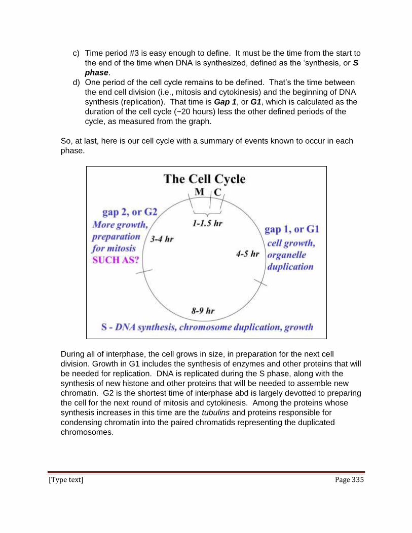
[Type text] Page 335

c) Time period #3 is easy enough to define. It must be the time from the start to

the end of the time when DNA is synthesized, defined as the ‘synthesis, or S

phase.

d) One period of the cell cycle remains to be defined. That’s the time between

the end cell division (i.e., mitosis and cytokinesis) and the beginning of DNA

synthesis (replication). That time is Gap 1, or G1, which is calculated as the

duration of the cell cycle (~20 hours) less the other defined periods of the

cycle, as measured from the graph.

So, at last, here is our cell cycle with a summary of events known to occur in each

phase.

During all of interphase, the cell grows in size, in preparation for the next cell

division. Growth in G1 includes the synthesis of enzymes and other proteins that will

be needed for replication. DNA is replicated during the S phase, along with the

synthesis of new histone and other proteins that will be needed to assemble new

chromatin. G2 is the shortest time of interphase abd is largely devotted to preparing

the cell for the next round of mitosis and cytokinesis. Among the proteins whose

synthesis increases in this time are the tubulins and proteins responsible for

condensing chromatin into the paired chromatids representing the duplicated

chromosomes.

[Type text] Page 336

Cohesin is a relatively recent example of a protein made in the run-up to mitosis. It

holds centromeres of chromatids together until they are ready to separate.

In a final note, typical dividing cells have generation times ranging from 16 to 24

hours. But some cells, like newly fertilized eggs might divide every hour or so. How

would you imagine a shortened cell cycle would look? How would events that

normally take a longer time occur in a much shorter time?

B. When cells stop dividing…

Cells that are terminally differentiated are those that will spend the rest of their lives

performing a specific function. These cells no longer cycle. Instead, shortly after

entering G1 they enter a phase called G0 (below).

Referred to as terminally differentiated, these cells will normally never divide

again. With a few exceptions (e.g., many neurons), most terminally differentiated

cells have a finite lifespan, and if necessary will be replaced by stem cells. Examples

include red blood cells; with a half-life of about 60 days, they are regularly replaced

by reticulocytes produced in bone marrow.

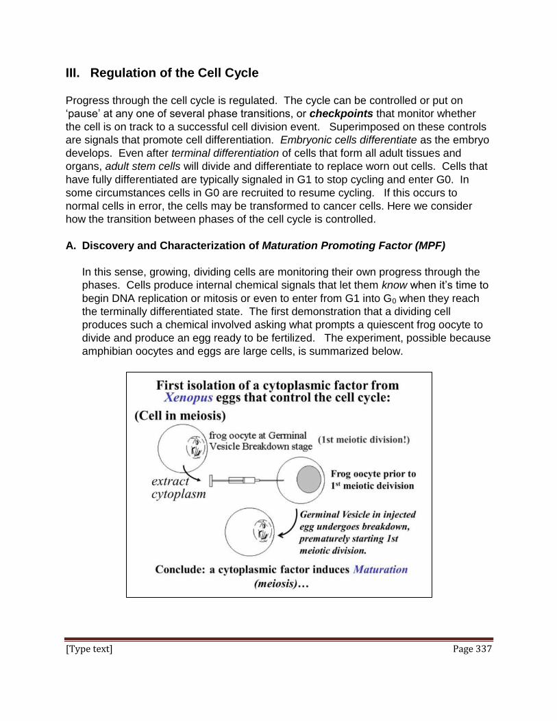
[Type text] Page 337

III. Regulation of the Cell Cycle

Progress through the cell cycle is regulated. The cycle can be controlled or put on

‘pause’ at any one of several phase transitions, or checkpoints that monitor whether

the cell is on track to a successful cell division event. Superimposed on these controls

are signals that promote cell differentiation. Embryonic cells differentiate as the embryo

develops. Even after terminal differentiation of cells that form all adult tissues and

organs, adult stem cells will divide and differentiate to replace worn out cells. Cells that

have fully differentiated are typically signaled in G1 to stop cycling and enter G0. In

some circumstances cells in G0 are recruited to resume cycling. If this occurs to

normal cells in error, the cells may be transformed to cancer cells. Here we consider

how the transition between phases of the cell cycle is controlled.

A. Discovery and Characterization of Maturation Promoting Factor (MPF)

In this sense, growing, dividing cells are monitoring their own progress through the

phases. Cells produce internal chemical signals that let them know when it’s time to

begin DNA replication or mitosis or even to enter from G1 into G0 when they reach

the terminally differentiated state. The first demonstration that a dividing cell

produces such a chemical involved asking what prompts a quiescent frog oocyte to

divide and produce an egg ready to be fertilized. The experiment, possible because

amphibian oocytes and eggs are large cells, is summarized below.

[Type text] Page 338

In this experiment, the hypothesis was that the cytoplasm of a frog oocyte in the

middle of meiosis must contain a chemical factor that caused the cell to lose its

nuclear membrane, condense its chromatin into chromosomes and enter meiosis.

Using a fine hypodermic needle, cytoplasm was withdrawn from these large oocytes

in the germinal vesicle breakdown stage, i.e., in the midst of the first meiotic division.

When this cytoplasm was transferred by injection into an oocyte not yet in meiosis,

the cell proceeded to enter meiosis prematurely. Clearly mature meiotic oocyte

cytoplasm contains a chemical factor that could be transferred from one cell to

another, inducing it to undergo meiosis. This chemical, called maturation

promoting factor (MPF) was isolated and purified from meiotic cells. When

injected into pre-meiotic cells, purified MPF caused them to enter meiosis (below).

[Type text] Page 339

MPF was subsequently shown to stimulate somatic cells in G2 to enter premature

mitosis; so conveniently, MPF can also be Mitosis Promoting Factor! Purified

MPF from meiotic or mitotic cells turns out to be a protein kinase made up of two

polypeptide subunits. When active, the kinase activity targets many cellular

proteins. One subunit contains the kinase enzyme active site and the other is a

regulatory polypeptide. To be an active kinase, both subunits must be bound.

Assays of MPF activity as well as the actual levels of the two subunits over time

during the cell cycle are shown below.

Based on the data, the regulatory subunit was called cyclin because its levels rise

gradually after cytokinesis, peaking at the next mitosis/meiosis. Levels of the kinase

subunit do not change during the life of the cell. Because its kinase activity required

cyclin, the subunit was called cyclin-dependent kinase (cdk). Note how MPF

enzyme activity and cyclin rise near the end of G2, peak in mitosis/meiosis and drop

precipitously thereafter. We now know as a cell approaches mitosis/meiosis, cyclin

binds to more and more cdk subunits, eventually reaching the threshold needed to

trigger entry into meiosis or mitosis.

[Type text] Page 340

B. Other Cyclins, CDKs and Cell Cycle Checkpoints

Other chemical signals accumulate at different points in the cell cycle. For example,

cells in S were fused with cells in G1), causing the G1 cells to begin synthesizing

DNA (visualized as 3H-thymine incorporation), as shown below.

In this case, an S-phase factor was isolated. This factor also turns out to be a two-

subunit protein kinase, albeit a different one from MPF. If the S-phase factor is not

produced during replication, the cell does not progress to G2. Unless these and

other regulatory cell cycle kinases are produced in cells at the right time, the cycle

would stall and the cells would not progress to the next phase. Together, these

kinases are part of a molecular sensing mechanism that act as checkpoints by

phosphorylating cytoplasmic and/or nuclear proteins involved in upcoming phases of

the cycle. Each of the factors will not be produced if the cells have not properly

completed the prior phase. And if any factor is not produced, the cells will be

arrested at one or another phase of the cell cycle.

[Type text] Page 341

The sequence of signals that control progress through the cell cycle is probably

more intricate and extensive than we currently know, but the three best described

checkpoints are in G1, G2 and M (below).

The G1 checkpoint is an interesting exception to the operation of “checkpoints” that

govern the forward progress of cycling cells. When cells in a tissue are fully

differentiated they are signaled to stop producing the active G1 checkpoint kinase.

These terminally differentiated cells do not progress beyond G1 into S. As we have

seen, these cells are instead arrested in G0. Let’s take a closer look at some events

that are being monitored at these checkpoints.

1. The G1 Checkpoint

We have already encountered the G1 (or ‘restriction’) checkpoint, which

determines whether cells will continue to the S phase. Cells will only progress to

the S phase if chemicals (mostly proteins) necessary for the replication process

are being made. These include enzymes of replication (DNA polymerases,

helicases, primases…) and others. Only when these molecules have

accumulated or become active at appropriate levels is it appropriate (and “safe”!)

to enter S.

2. The G2 Checkpoint

Passage through the G2 checkpoint is only possible if DNA made in the prior S

phase is not damaged, or if it was, that the damage has been or can be repaired

(e.g., by proofreading functions of replication). Cells that pass the G2 checkpoint

have active genes allowing accumulation of proteins that will be needed for

[Type text] Page 342

mitosis, such as nuclear proteins necessary to condense chromatin into

chromosomes, tubulins for making microtubules, etc. Only when levels of these

and other required proteins reach a threshold can the cell begin mitosis.

3. M Checkpoint

This is the checkpoint governed by the original MPF. It functions at metaphase,

phosphorylating proteins that bind to chromatin causing it to condense and form

chromatids. MPF-catalyzed phosphorylation also enables spindle fiber formation

and the breakdown of the nuclear envelope. At metaphase, tension developed in

the spindle apparatus tugs at the kinetochores holding the duplicated chromatids

together. When this tension reaches a threshold level, MPF peaks and an active

separase is produced causing the chromatids to separate. The tension in the

spindle apparatus becomes the force that separates the new chromosomes in

anaphase. At this time, proteins phosphorylated by MPF even initiate the

breakdown of cyclin in the cell. Passing the M checkpoint means that the cell will

complete mitosis (anaphase and telophase) and cytokinesis, and that each

daughter cell will enter a new G1 phase.

4. The G0 State

This is not really a phase of the cell cycle, since cells in G0 have reached a

terminally differentiated state and stopped dividing. In development this means

that the formation of a tissue or an organ is complete. Some cells live short lives

in G0 (e.g., some embryonic cells), and others live so long in G0 that they are

seldom if ever replaced (muscle cells, neurons). An example of a differentiated

cell type that can be normally reactivated from G0 is the lymphocyte, an immune

system white blood cell. Exposure to foreign chemicals or pathogens activates

lymphocytes to re-enter the cell cycle where the newly divided cells make the

antibodies that neutralize the chemicals and fight off the pathogens. On the

other hand, if cells are unable to enter G0 when they are supposed to, or if they

are inappropriately signaled to exit G0, they will re-enter the cell cycle. Such cells

have escaped the checkpoints and controls on cell division, and may become the

focal point of tumor and other cancer cell growth.

Dividing yeast cells seem to have only the three checkpoints discussed here. More

complex eukaryotes have more cell cycle controls, including more cyclins, more

cdks and consequently, more checkpoints. Cyclins are conserved proteins encoded

by related genes. Like the one in MPF, these cyclins are characterized by cyclic

patterns of synthesis. Likewise, cdks are also encoded by evolutionarily conserved

genes, and are maintained at constant levels throughout the cell cycle. Each kinase

holoprotein (cyclin-bound cdk) is different, catalyzing the phosphorylation of sets of

cellular proteins specific to each phase of the cell cycle.

[Type text] Page 343

C. When Cells Die

As noted, few cell types live forever, and most live for a finite time. These cells are

destined to turn over (another euphemism for dying). This programmed cell death is

called Apoptosis. It occurs during normal development when cells are temporarily

required for a maturation process (e.g., embryo formation, metamorphosis). When

these cells are no longer necessary, or when a genetically or otherwise damaged

cell is detected in a population of dividing cells, they undergo apoptosis.

Programmed cell death often starts with an external signal programmed to appear at

a specific time in development. The signal molecule acts on target cells to induce

transcription of the Bcl2 gene. The Bcl2 proteins Bak and Bax are outer

mitochondrial membrane channel components that will allow the organelles to

release cytochrome C, setting off the sequence of molecular events leading to

apoptosis. This is animated at http://youtu.be/QL7M_j4LjVc. The effects of

cytochrome C in the cytoplasm are illustrated below and animated at

http://youtu.be/x3-ZKUbY_SY.

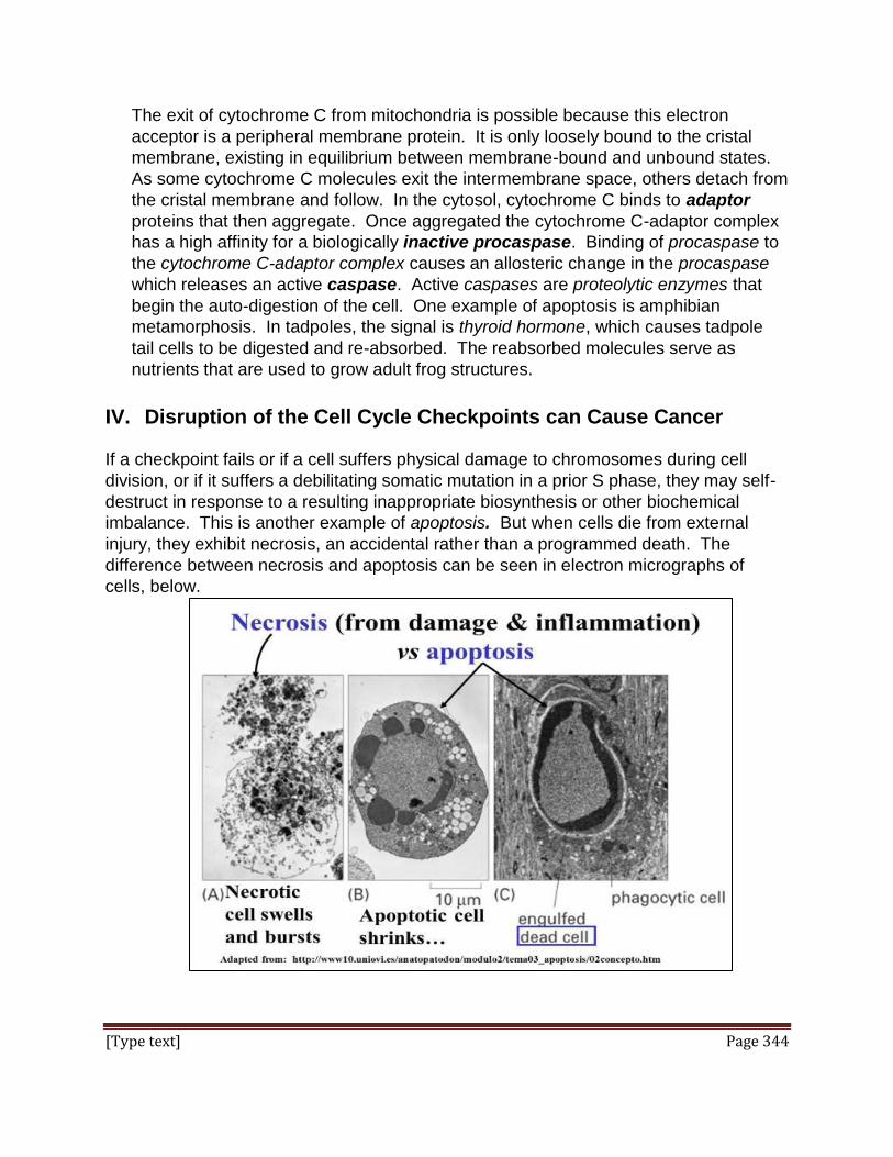
[Type text] Page 344

The exit of cytochrome C from mitochondria is possible because this electron

acceptor is a peripheral membrane protein. It is only loosely bound to the cristal

membrane, existing in equilibrium between membrane-bound and unbound states.

As some cytochrome C molecules exit the intermembrane space, others detach from

the cristal membrane and follow. In the cytosol, cytochrome C binds to adaptor

proteins that then aggregate. Once aggregated the cytochrome C-adaptor complex

has a high affinity for a biologically inactive procaspase. Binding of procaspase to

the cytochrome C-adaptor complex causes an allosteric change in the procaspase

which releases an active caspase. Active caspases are proteolytic enzymes that

begin the auto-digestion of the cell. One example of apoptosis is amphibian

metamorphosis. In tadpoles, the signal is thyroid hormone, which causes tadpole

tail cells to be digested and re-absorbed. The reabsorbed molecules serve as

nutrients that are used to grow adult frog structures.

IV. Disruption of the Cell Cycle Checkpoints can Cause Cancer

If a checkpoint fails or if a cell suffers physical damage to chromosomes during cell

division, or if it suffers a debilitating somatic mutation in a prior S phase, they may self-

destruct in response to a resulting inappropriate biosynthesis or other biochemical

imbalance. This is another example of apoptosis. But when cells die from external

injury, they exhibit necrosis, an accidental rather than a programmed death. The

difference between necrosis and apoptosis can be seen in electron micrographs of

cells, below.

[Type text] Page 345

In the normal course of events, cycling cells continue to divide until they attain G0 in the

terminally differentiated state. We noted that most terminally differentiated cells have a

finite lifespan in an organism, to be cleared by apoptosis and replaced by stem cells.

We also noted that accidental signaling can bring cells out of G0, leading to renewed cell

proliferation. While these cells are obviously abnormal, they are not detected by

apoptotic defense mechanisms, so that they undergo uncontrolled cell divisions to

become cancer cells. Likewise, physically damaged cells or cells with certain kinds of

mutations may sometimes escape clearance by apoptosis. When they do, they may

also become cancer cells. Apoptotic clearance and the uncontrolled proliferation of

cancer cells are shown below.

From: Normal_cancer_cell_division_from_NIH.png

[Type text] Page 346

A. Somatic Mutations that Can Lead to Deregulation of the Cell Cycle

Cancerous growth could result for example if a normal dividing cell should suffer a

somatic mutation such that a cdk is over-expressed. And if cyclin levels in daughter

cells fail to drop, the cell would not be able to stop cycling. Likewise, a cell in G0

might be stimulated to begin cycling again by an inappropriate encounter with a

hormone or other signal. These are examples of anomalies that if undetected can

transform cells to cancer cells. Thus cancer cells arise when mutations eliminate a

cell cycle checkpoint, or when inappropriate timing of cell signaling fools a quiescent

cell into resuming cell divisions. Uncontrolled cell growth is an apt description of

cancer cell growth, since their normal cycling has been deregulated.

B. Growth and Behavior of Cancer Cells

Different cancer cell types have different growth and other behavioral properties.

You may have heard of slow growing and fast growing cancers. Colon cancers

are typically slow growing. In middle-age or older people, periodic colonoscopies

can detect and remove colorectal tumors. Pancreatic cancers are fast growing and

often go undetected until they reach an advanced stage. The twin goals of medical

research are to detect the different cancers early enough for successful intervention,

and of course to find effective treatments.

A single mutated cell in a tissue can become the growth point of a tumor, essentially

a mass of cells cloned from the original mutated one. Benign tumors or growths

(for example breast and uterine fibroids in women, or common moles) stop growing

and are not life threatening. They are often surgically removed for the comfort of the

patient (or because cells in some otherwise benign tumors have a potential to

become cancerous). Malignant tumors (also called malignant neoplasms) are

cancerous and can grow beyond the boundaries of the tumor itself. When tumor

cells are shed they may enter the bloodstream and travel to other parts of the body

(the phenomenon called metastasis), where they can initiate the growth of more

tumors. Because cancer cells continue to cycle and replicate their DNA, they can

undergo additional somatic mutations. These further changes can facilitate

metastasis and cancer cell growth in different locations in the body.

C. Cancer Treatment Strategies

There are many different kinds of cancers originating in different tissues of the body.

They all share the property of uncontrolled cell division, albeit for different molecular

and not well known reasons. The two major treatment strategies for cancers all aim

[Type text] Page 347

at disrupting replication in some way. For example, radiation therapy aims

mutagenic radiation at tumors in the hope that replicating DNA will be mutated at so

many sites (i.e., genes) that they can no longer survive. Some tumors do not

respond well to radiation (or can’t easily be reached by radiation technologies), and

some cancers do not even form focused tumors (for example lymphomas and

leukemias involving lymph and blood cells). These are treated by chemotherapy,

which also aims to derange replication or mitotic activities. One of the

dideoxynucleotides we saw used in the Sanger method of DNA sequencing, ddCTP

is in fact a chemotherapeutic agent (called cordycepin) because once it is

incorporated into a growing DNA chain during replication, no additional nucleotides

can be added to the DNA strand. Taxol is another chemo drug that acts by blocking

spindle fiber microtubules from depolymerizing, thus blocking mitosis. These

therapies are not necessarily specific for cancer cell types. When they are

successful it is because cancer cells proliferate rapidly and constantly while other

cell types do not.

The message you should be getting is that we have a long way to go before we

develop cancer therapies that target specific cancers rather than spraying shotgun

pellets at the DNA of all dividing cells. Many if not all of the side effects of radiation

and chemical therapies result from the damage these treatments do to normal

dividing cells (e.g., hair follicle cells accounting for hair loss among many cancer

patients, depletion of blood cells that fail to be replaced by stem cells in bone

marrow). So, we must wait for more specific cancer treatments, perhaps

immunotherapies that will recognize only cancer and not normal cells.

Some iText & VOP Key Words and Terms

anaphase G0 of the cell cycle mitosis

apoptosis G1 checkpoint mitosis promoting factor

benign tumors G1 phase mitotic phases

cancer cells G2 checkpoint MPF

CDKs G2 phase mTOR signaling

cell cycle interphase necrosis

[Type text] Page 348

cell cycle checkpoints invasive tumors programmed cell death

chemotherapy M checkpoint prophase

colchicine M phase of the cell cycle protein phosphorylation

cyclin level in cell cycle malignant tumors radiation therapy

cyclin-dependent kinases maturation S phase

cyclin maturation promoting factor Taxol

cytokinesis metaphase telophase

dideoxyNTP chemotherapy metastasis

[Type text] Page 349

List of Videos on Youtube

Videos Embedded in the iText (02-04-2015) http://youtu.be/cpps2CZ0aA4 Calorimetry http://youtu.be/BLEB0A_9Tt4 PSI photosynthesis clip http://youtu.be/t4RlsDDsNi8 Z Scheme of Photosynthesis http://youtu.be/T6HfiwC0euI Cyclic Photophosphorylation http://youtu.be/XtzExh3I17c Dark reactions photosynthesis http://youtu.be/29gFdfhtmYk E. coli Replication Initiation http://youtu.be/xdm4UpixaLU Telomerase action http://youtu.be/ThMSjtggNDo Processive Replication http://youtu.be/UN56se_-yfY snRNPs and mRNA splicing http://youtu.be/jpHSgq1MIPg rRNA ribosome assembly and export http://youtu.be/0m-PXfWWxNA mRNA-30S subunit association http://youtu.be/KoU9y3W3wsk Translation Initiation Complex formation http://youtu.be/swy_qV6_Fb8 Translation Elongation http://youtu.be/YN3qUL5svnQ lac operon transcription & translation http://youtu.be/RKf66-VzYI0 Basic lac operon transcription http://youtu.be/MNQ8CzhDfCg lac Operon Derepression http://youtu.be/G590s9xZ9VA Transcription Regulation by Steroid Hormones http://youtu.be/CSvNSm7pqyc Signal Transduction Pathways http://youtu.be/21C01D2Tgeg miRNAs http://youtu.be/BTAi3RoSkV0W siRNA Pathway http://youtu.be/Hp0OFPV62y0 Translational control of globin gene expression by Hemin http://youtu.be/_g-DQq4XDfw Proteasome-Ubiquitin Action http://youtu.be/_z-ydn718yM Make Recombinant Plasmids-Transform Bacteria http://youtu.be/nemMygDhMLc Replica plating to identify recombinant clones http://youtu.be/p2zxwQl8n9s Microarray Robotics http://youtu.be/oGsET23q-e0 Demonstrating a Fluid Mosaic Membrane http://youtu.be/TkHNC8ePMPE Making Cell Surface Glycoproteins http://youtu.be/1PPz5kzOChg Diffusion Across Membranes http://youtu.be/OEFUvF56deU Glucose Transport vs. Symport http://youtu.be/SXL1RBK3Rm8 Facilitated Diffusion http://youtu.be/-xZvya2Gt50 [Na+][K+] Pump http://youtu.be/tSks9WPDxHM Ion Channels in Neurotransmission http://youtu.be/csQ_-e92C-Q COPs and SNARES http://youtu.be/vgZHf_Ju-PQ Importing Proteins to Nucleus http://youtu.be/cTlu79rhJYs Mitochondrial Protein Import http://youtu.be/Se9N5sKmYcE G-Protein Signaling http://youtu.be/fz9Irqm0lyg Fight or Flight Amplification Cascade http://youtu.be/Czs2hIWvCQQ Receptor Kinase Ligand Binding http://youtu.be/FjS6HtpLOgE Receptor Tyrosine Kinase Activation http://youtu.be/m9cVMHFKDhY Receptor Kinase e.g., Mitogenic Pathway http://youtu.be/CkeYBSD9RJg Microtubule Polarity Experiment http://youtu.be/1PSenpp7TmE Spindle Fibers Exert Force on Chromatids http://youtu.be/Y6RBJfUpZec Sliding Microtubules http://youtu.be/zsKhdjIAw8s Reconstituted Sarcomere Contraction http://youtu.be/CrB7A_DAk3I Myosin Head Allostery During Sliding Along Actin http://youtu.be/HpZpA-vYDBU Calcium Release from Sarcoplasmic Reticulum http://youtu.be/LvDSi7xtdYo Actin and Cytokinesis http://youtu.be/QL7M_j4LjVc Bcl2 Gene Activation in Apoptosis http://youtu.be/x3-ZKUbY_SY Caspase Activation leads to Apoptosis

[Type text] Page 350

Videos associated with Instructor Annotations

http://youtu.be/g6Ra9_c2IaQ Polar H2O http://youtu.be/qPgZnmVFv8g Thermodynamic Laws http://youtu.be/27B0D1uf8GM Enthalpy http://youtu.be/PwLbYYyudZA Electron Flow in ET… http://youtu.be/p_c7VJvqEbo Prescott Experiment http://youtu.be/BLvXIoKh8uI Propagation of an Action Potential http://youtu.be/SlM6U0Y6BxQ Endomembranes in Action http://youtu.be/Bw23E7e0YNk ID EM Nuclei http://youtu.be/oZX1H0X7xQY Phase Contrast Micrograph of Isolated Chloroplasts http://youtu.be/BCsGqmO35BY Calorimeter Experiment http://youtu.be/gKSFLTyyzEI Reduction Potentials… http://youtu.be/51sT-3YU9yk Semicon Replication… http://youtu.be/_c_JCjYrTZM Eukaryotic Replicons in S Phase http://youtu.be/KgNjHunG79M Restriction Map Experiment http://youtu.be/9Qp3Ff90K_A Microarray Question http://youtu.be/qgkwqly-ROE Channel States in an Action Potential