cell-aware fault analysis and test set optimization in

Southern Methodist UniversitySMU ScholarComputer Science and Engineering Theses andDissertations Computer Science and Engineering

Spring 5-19-2018

Cell-Aware Fault Analysis and Test SetOptimization in Digital Integrated CircuitsFanchen ZhangSouthern Methodist University, [email protected]

Jennifer DworakSouthern Methodist University, [email protected]

Follow this and additional works at: https://scholar.smu.edu/engineering_compsci_etds

Part of the Electronic Devices and Semiconductor Manufacturing Commons

This Dissertation is brought to you for free and open access by the Computer Science and Engineering at SMU Scholar. It has been accepted forinclusion in Computer Science and Engineering Theses and Dissertations by an authorized administrator of SMU Scholar. For more information,please visit http://digitalrepository.smu.edu.

Recommended CitationZhang, Fanchen and Dworak, Jennifer, "Cell-Aware Fault Analysis and Test Set Optimization in Digital Integrated Circuits" (2018).Computer Science and Engineering Theses and Dissertations. 4.https://scholar.smu.edu/engineering_compsci_etds/4

https://scholar.smu.edu?utm_source=scholar.smu.edu%2Fengineering_compsci_etds%2F4&utm_medium=PDF&utm_campaign=PDFCoverPages

https://scholar.smu.edu/engineering_compsci_etds?utm_source=scholar.smu.edu%2Fengineering_compsci_etds%2F4&utm_medium=PDF&utm_campaign=PDFCoverPages


https://scholar.smu.edu/engineering_compsci?utm_source=scholar.smu.edu%2Fengineering_compsci_etds%2F4&utm_medium=PDF&utm_campaign=PDFCoverPages


http://network.bepress.com/hgg/discipline/272?utm_source=scholar.smu.edu%2Fengineering_compsci_etds%2F4&utm_medium=PDF&utm_campaign=PDFCoverPages

https://scholar.smu.edu/engineering_compsci_etds/4?utm_source=scholar.smu.edu%2Fengineering_compsci_etds%2F4&utm_medium=PDF&utm_campaign=PDFCoverPages

http://digitalrepository.smu.edu

CELL-AWARE FAULT ANALYSIS AND

TEST SET OPTIMIZATION

IN DIGITAL INTEGRATED CIRCUITS

Approved by:

Dr. Jennifer Dworak

Associate Professor

Dr. Ping Gui

Professor

Dr. LiGuo Huang

Associate Professor

Dr. Theodore Manikas

Clinical Professor

Dr. Sukumaran Nair

Professor

Dr. Kundan Nepal

Associate Professor

CELL-AWARE FAULT ANALYSIS AND

TEST SET OPTIMIZATION

IN DIGITAL INTEGRATED CIRCUITS

A Dissertation Presented to the Graduate Faculty of the

Lyle School

Southern Methodist University

in

Partial Fulfillment of the Requirements

for the degree of

Doctor of Philosophy

with a

Major in Computer Engineering

by

Fanchen Zhang

B.A., Telecommunication Engineering, Harbin Institute of Technology, ChinaM.S., Electrical Engineering, Southern Methodist University

May 19, 2018

Copyright (2018)

Fanchen Zhang

All Rights Reserved

iii

ACKNOWLEDGMENTS

This work could not have been accomplished by the wisdom of my wonderful advisor,

Prof. Dworak, along with her many colleagues in the Department of Computer Science

here at SMU. I would like to express sincere acknowledgement to labmates Allison Garcia,

Micah Thornton, Daphne Hwong, Yi Sun, and Soha Alhelaly for their dedicated work to

these projects. I am thankful for Geoff Shofner and LeRoy Winemberg for their industrial

suggestion to lead projects to be practicabililty. I’m also forever grateful to my family for

being so patient with me and my friends for reminding me to take breaks and go be great

instead of just reading about greatness all of the time.

iii

Zhang, Fanchen B.A., Telecommunication Engineering, Harbin Institute of Technology, ChinaM.S., Electrical Engineering, Southern Methodist University

Cell-Aware Fault Analysis and

Test Set Optimization

in Digital Integrated Circuits

Advisor: Dr. Jennifer Dworak

Doctor of Philosophy degree conferred May 19, 2018

Dissertation completed May 10, 2018

Structural tests have many advantages over functional patterns. The fault coverage

of structural patterns is generally higher and easier to quantify, well-known algorithms are

available to generate them, and they are often a much easier choice for debugging and

diagnosis. However, depending on the fault models used,traditional structural patterns can

still miss many defects, such as the defects that may occur inside the standard cells, and

when chips are placed on a board, they may fail in functional mode even if they pass all

structural tests. This can happen even if those same structural tests are applied in-system

on the board, making debug very difficult.

Cell-aware faults have been proposed to model those defects inside the standard cells

and allow ATPG tools to target them. In some cases, for small circuits, the test set is

reasonably short. However, for industrial circuits, the test sets that obtain 100% cell-aware

fault coverage are often much too long to be applied efficiently. One previous study has

shown that the increase in test pattern count may be more than 50% to 80%.

The goal of this research is to reduce the time required to apply test sets capable of of

detecting cell-aware faults. In this dissertation, we explore an approach that involves the

insertion of Design for Testability (DFT) logic into the circuit to utilize the wasted scan-

shift clock cycles to enhance the fortuitous detections of cell-aware faults. In particular, we

consider an approach that allows data to be captured in shadow flip-flops during scan shift,

where those flip-flops have been collected into a MISR (Multiple Input Signature Register)

iv

to allow a single signature to be obtained.

In this investigation, we initially fault simulated all scan-shift clock cycles for a given

stuck-at fault test set to determine which flip-flops should be shadowed and included in

the MISR. Unfortunately, fault simulating this many patterns is very time consuming and

may be impractical for large circuits—especially if the scan chains are also long. This fault

simulation is also needed to identify which cell-aware faults may still be missed by the

intermediate shift patterns so that additional top-off patterns may be added. Finally, the

area overhead required to maximize cell-aware fault detection using shadow flops may be

prohibitive for some circuits.

To resolve these issues, we considered several optimizations. First, we use scan shift cycle

sampling to reduce the fault simulation time, and we designed a MISR capture controller

to allow scan shift capture to happen at regular intervals. Second, we use fault cones to

predict which flip-flops should be shadowed without doing any fault simulation. Finally,

we explored algorithms for selecting shadow flops to best trade off additional fault coverage

with additional area overhead and further reduced test set size by using a heuristic that

iteratively ran ATPG multiple times with varying fault lists.

v

TABLE OF CONTENTS

LIST OF FIGURES . . . . . . . . . . . . . . . . . . . . . . . . . . . . . . . . . . . . . . . . . . . . . . . . . . . . . . . . . . . . . . . . . x

LIST OF TABLES . . . . . . . . . . . . . . . . . . . . . . . . . . . . . . . . . . . . . . . . . . . . . . . . . . . . . . . . . . . . . . . . . . xiv

CHAPTER

1. INTRODUCTION . . . . . . . . . . . . . . . . . . . . . . . . . . . . . . . . . . . . . . . . . . . . . . . . . . . . . . . . . . . . 1

1.1. Manufacturing Test . . . . . . . . . . . . . . . . . . . . . . . . . . . . . . . . . . . . . . . . . . . . . . . . . . . . . . 1

1.1.1. The Role of Testing in VLSI Circuit Manufacturing . . . . . . . . . . . . . . . . 1

1.1.2. Basic Digital Testing . . . . . . . . . . . . . . . . . . . . . . . . . . . . . . . . . . . . . . . . . . . . . . 1

1.1.3. The Challenges for Testing . . . . . . . . . . . . . . . . . . . . . . . . . . . . . . . . . . . . . . . . 2

1.2. Motivation . . . . . . . . . . . . . . . . . . . . . . . . . . . . . . . . . . . . . . . . . . . . . . . . . . . . . . . . . . . . . . . 4

1.3. Main Contributions . . . . . . . . . . . . . . . . . . . . . . . . . . . . . . . . . . . . . . . . . . . . . . . . . . . . . . 6

2. BACKGROUND . . . . . . . . . . . . . . . . . . . . . . . . . . . . . . . . . . . . . . . . . . . . . . . . . . . . . . . . . . . . . . 9

2.1. Functional vs. Structural Testing . . . . . . . . . . . . . . . . . . . . . . . . . . . . . . . . . . . . . . . . . 9

2.1.1. Functional Test . . . . . . . . . . . . . . . . . . . . . . . . . . . . . . . . . . . . . . . . . . . . . . . . . . . 9

2.1.2. Structural Test . . . . . . . . . . . . . . . . . . . . . . . . . . . . . . . . . . . . . . . . . . . . . . . . . . . . 9

2.2. Fault Models . . . . . . . . . . . . . . . . . . . . . . . . . . . . . . . . . . . . . . . . . . . . . . . . . . . . . . . . . . . . . 10

2.2.1. Single Stuck-at Fault Model . . . . . . . . . . . . . . . . . . . . . . . . . . . . . . . . . . . . . . . 11

2.2.2. Transition Fault Model . . . . . . . . . . . . . . . . . . . . . . . . . . . . . . . . . . . . . . . . . . . . 12

2.2.3. Cell-aware Fault Model . . . . . . . . . . . . . . . . . . . . . . . . . . . . . . . . . . . . . . . . . . . . 13

2.3. Test Set Generation . . . . . . . . . . . . . . . . . . . . . . . . . . . . . . . . . . . . . . . . . . . . . . . . . . . . . . 14

2.3.1. Probabilistic . . . . . . . . . . . . . . . . . . . . . . . . . . . . . . . . . . . . . . . . . . . . . . . . . . . . . . 15

2.3.1.1. N-detect . . . . . . . . . . . . . . . . . . . . . . . . . . . . . . . . . . . . . . . . . . . . . . . . . 15

2.3.1.2. Gate Exhaustive . . . . . . . . . . . . . . . . . . . . . . . . . . . . . . . . . . . . . . . . . 15

2.3.1.3. Random Test and Logic BIST . . . . . . . . . . . . . . . . . . . . . . . . . . . . 16

vi

2.3.2. Deterministic . . . . . . . . . . . . . . . . . . . . . . . . . . . . . . . . . . . . . . . . . . . . . . . . . . . . . 19

2.3.2.1. Automatic Test-Pattern Generator . . . . . . . . . . . . . . . . . . . . . . . 19

2.3.2.2. Fault Cones . . . . . . . . . . . . . . . . . . . . . . . . . . . . . . . . . . . . . . . . . . . . . . 20

2.3.2.3. Scan-Chain . . . . . . . . . . . . . . . . . . . . . . . . . . . . . . . . . . . . . . . . . . . . . . 20

3. FUNCTIONAL VS. NONFUNCTIONAL FAULT DETECTION . . . . . . . . . . . . . . . 24

3.1. Sub-Gate-Exhaustive Faults And Their Relation To Stuck-at ATPG . . . . . . . 25

3.1.1. The Reasoning Behind N-detect Test Sets . . . . . . . . . . . . . . . . . . . . . . . . . 27

3.1.2. Experiments for Sub-Gate-Exhaustive Fault Detection by N -detect Test Patterns. . . . . . . . . . . . . . . . . . . . . . . . . . . . . . . . . . . . . . . . . . . . . . . 28

3.1.3. Determing which Sub-Gate-Exhaustive Faults to Target . . . . . . . . . . . . 31

3.2. Summary . . . . . . . . . . . . . . . . . . . . . . . . . . . . . . . . . . . . . . . . . . . . . . . . . . . . . . . . . . . . . . . . 41

4. CHARACTERIZATION OF CELL-AWARE FAULT DETECTABILITY . . . . . . . 43

4.1. Background . . . . . . . . . . . . . . . . . . . . . . . . . . . . . . . . . . . . . . . . . . . . . . . . . . . . . . . . . . . . . . 43

4.2. Extracting Layout-Based Cell-Aware-Type Faults from Cell-Aware ATPGof Standard Cells . . . . . . . . . . . . . . . . . . . . . . . . . . . . . . . . . . . . . . . . . . . . . . . . . . . . . . . . . 44

4.3. Exploring the Additional Patterns Required for Static Cell-Aware FaultDetections at the Standard Cell Level . . . . . . . . . . . . . . . . . . . . . . . . . . . . . . . . . . . . . 45

4.4. Exploring the Additional Patterns Required for Delay-Based Cell-AwareFault Detections at the Standard Cell Level . . . . . . . . . . . . . . . . . . . . . . . . . . . . . . . 52

4.5. Summary and Next Work . . . . . . . . . . . . . . . . . . . . . . . . . . . . . . . . . . . . . . . . . . . . . . . . 52

5. PUTTING WASTED CLOCK CYCLES TO USE: ENHANCING FORTU-

ITOUS CELL-AWARE FAULT DETECTION WITH SCAN SHIFT CAPTURE 57

5.1. Background and Related Work . . . . . . . . . . . . . . . . . . . . . . . . . . . . . . . . . . . . . . . . . . . 58

5.2. Capturing Test Results on Scan Shift . . . . . . . . . . . . . . . . . . . . . . . . . . . . . . . . . . . . . 59

5.3. Experimental Setup . . . . . . . . . . . . . . . . . . . . . . . . . . . . . . . . . . . . . . . . . . . . . . . . . . . . . . 62

5.3.1. Defining Intermediate Shift Patterns . . . . . . . . . . . . . . . . . . . . . . . . . . . . . . . 63

5.3.2. Handling Chains of Different Lengths . . . . . . . . . . . . . . . . . . . . . . . . . . . . . . 66

vii

5.3.3. Handling X’s in Capture Values . . . . . . . . . . . . . . . . . . . . . . . . . . . . . . . . . . . 66

5.4. Experimental Results . . . . . . . . . . . . . . . . . . . . . . . . . . . . . . . . . . . . . . . . . . . . . . . . . . . . . 67

5.4.1. Fortuitous Cell-Aware Fault Detectionby Intermediate Scan ShiftPatterns . . . . . . . . . . . . . . . . . . . . . . . . . . . . . . . . . . . . . . . . . . . . . . . . . . . . . . . . . . 67

5.4.2. Test Set Size Reduction . . . . . . . . . . . . . . . . . . . . . . . . . . . . . . . . . . . . . . . . . . . 68

5.4.3. Area Overhead . . . . . . . . . . . . . . . . . . . . . . . . . . . . . . . . . . . . . . . . . . . . . . . . . . . . 68

5.4.4. Intermediate Shift Cycles Needed for Capture . . . . . . . . . . . . . . . . . . . . . . 71

5.4.5. MISR Aliasing . . . . . . . . . . . . . . . . . . . . . . . . . . . . . . . . . . . . . . . . . . . . . . . . . . . . 73

5.4.6. Reducing the Stuck-at Fault Test Set . . . . . . . . . . . . . . . . . . . . . . . . . . . . . . 73

5.5. Summary . . . . . . . . . . . . . . . . . . . . . . . . . . . . . . . . . . . . . . . . . . . . . . . . . . . . . . . . . . . . . . . . 77

6. OPTIMIZATIONS FOR REDUCED AREA OVERHEAD AND FAULT SIM-

ULATION TIME. . . . . . . . . . . . . . . . . . . . . . . . . . . . . . . . . . . . . . . . . . . . . . . . . . . . . . . . . . . . . . 78

6.1. Sampling Intermediate Shift Cycles . . . . . . . . . . . . . . . . . . . . . . . . . . . . . . . . . . . . . . . 79

6.1.1. On-chip Circuitry for Shift Cycle Capture . . . . . . . . . . . . . . . . . . . . . . . . . 80

6.1.2. Fortuitous Cell-Aware Fault Detection by Intermediate Scan ShiftPatterns at Different Sampling Rates . . . . . . . . . . . . . . . . . . . . . . . . . . . . . . 81

6.1.3. Test Set Size Reduction with Shift Cycle Sampling . . . . . . . . . . . . . . . . . 83

6.1.4. Area Overhead with Scan Shift Sampling . . . . . . . . . . . . . . . . . . . . . . . . . . 84

6.1.5. Intermediate Shift Cycles Needed for Capture . . . . . . . . . . . . . . . . . . . . . . 85

6.1.6. MISR Aliasing . . . . . . . . . . . . . . . . . . . . . . . . . . . . . . . . . . . . . . . . . . . . . . . . . . . . 87

6.2. Tradeoff between the size of the test set and the shadow flop overhead . . . . . 87

6.3. Summary . . . . . . . . . . . . . . . . . . . . . . . . . . . . . . . . . . . . . . . . . . . . . . . . . . . . . . . . . . . . . . . . 91

7. ATPG TEST SET REDUCTION USING SCAN SHIFT CAPTURE WITH

FAULT CONES TO SELECT SHADOW FLOPS . . . . . . . . . . . . . . . . . . . . . . . . . . . . . . 92

7.1. Selecting Shadow Flip-Flops Using Fault Cone . . . . . . . . . . . . . . . . . . . . . . . . . . . . 92

7.2. Iterative Test Pattern Generation . . . . . . . . . . . . . . . . . . . . . . . . . . . . . . . . . . . . . . . . . 94

7.3. Experimental Results . . . . . . . . . . . . . . . . . . . . . . . . . . . . . . . . . . . . . . . . . . . . . . . . . . . . . 97

viii

7.4. Summary . . . . . . . . . . . . . . . . . . . . . . . . . . . . . . . . . . . . . . . . . . . . . . . . . . . . . . . . . . . . . . . . 99

8. CONCLUSION. . . . . . . . . . . . . . . . . . . . . . . . . . . . . . . . . . . . . . . . . . . . . . . . . . . . . . . . . . . . . . . . 101

APPENDIX

BIBLIOGRAPHY . . . . . . . . . . . . . . . . . . . . . . . . . . . . . . . . . . . . . . . . . . . . . . . . . . . . . . . . . . . . . . . . . . . 104

ix

LIST OF FIGURES

Figure Page

1.1 Conceptual approach used for digital testing . . . . . . . . . . . . . . . . . . . . . . . . . . . . . . . . . . 2

1.2 Possible testing outcomes . . . . . . . . . . . . . . . . . . . . . . . . . . . . . . . . . . . . . . . . . . . . . . . . . . . . 3

2.1 A half adder with a single stuck-at fault . . . . . . . . . . . . . . . . . . . . . . . . . . . . . . . . . . . . . . 12

2.2 BIST architecture in the high level . . . . . . . . . . . . . . . . . . . . . . . . . . . . . . . . . . . . . . . . . . . 16

2.3 LFSR with third degree polynomial . . . . . . . . . . . . . . . . . . . . . . . . . . . . . . . . . . . . . . . . . . 17

2.4 Multiple Input Signature Register (MISR) . . . . . . . . . . . . . . . . . . . . . . . . . . . . . . . . . . . . 18

2.5 One of stuck-at fault test pattern . . . . . . . . . . . . . . . . . . . . . . . . . . . . . . . . . . . . . . . . . . . . . 19

2.6 Faults and fault cones . . . . . . . . . . . . . . . . . . . . . . . . . . . . . . . . . . . . . . . . . . . . . . . . . . . . . . . . 21

2.7 Scan chain . . . . . . . . . . . . . . . . . . . . . . . . . . . . . . . . . . . . . . . . . . . . . . . . . . . . . . . . . . . . . . . . . . . 21

2.8 Scan flip-flop . . . . . . . . . . . . . . . . . . . . . . . . . . . . . . . . . . . . . . . . . . . . . . . . . . . . . . . . . . . . . . . . . 22

3.1 Mandatory and non-mandatory input combinations for full stuck-at faultcoverage. . . . . . . . . . . . . . . . . . . . . . . . . . . . . . . . . . . . . . . . . . . . . . . . . . . . . . . . . . . . . . . . . . 26

3.2 Test Patterns Required for Stuck-at and Sub-Gate-Exhuastive Faults forSub-Gate-Exhuastive Fault Set 1 and Good State Set 1 . . . . . . . . . . . . . . . . . . . . 30


3.4 Overall flow for determining which sub-gate-exhaustive faults are function-ally important for one set of sub-gate-exhaustive faults and one-set-ofgood states. This flow is repeated four times: for two fault lists and twosets of good states. . . . . . . . . . . . . . . . . . . . . . . . . . . . . . . . . . . . . . . . . . . . . . . . . . . . . . . . 33



x

3.7 Percent Increase in Test Set Length when Potentially Non-Functional Sub-Gate-Exhaustive Faults are Targeted for Sub-Gate-Exhaustive Fault Set1 and Good State Set 1 . . . . . . . . . . . . . . . . . . . . . . . . . . . . . . . . . . . . . . . . . . . . . . . . . . . 37




3.11 Distribution of Sub-Gate-Exhaustive Faults Between Functional & Non-Functional for those not Detected by Stuck-At ATPG for Cell-AwareFault Set 1 and Good State Set 1 . . . . . . . . . . . . . . . . . . . . . . . . . . . . . . . . . . . . . . . . . 39




4.1 Flowchart for obtaining data regarding test patterns obtained by targetingcell-aware faults and stuck-at or transition faults . . . . . . . . . . . . . . . . . . . . . . . . . . 45

4.2 Comparison between the number of test patterns required for compressedtest sets covering different types static faults for NanGateTM library . . . . . . . 46

4.3 Comparison between the number of test patterns required for compressedtest sets covering different types of static faults for the commercial library . . 47

4.4 Comparison between the number of test patterns required for compressedtest sets covering different types static faults without gate exhuastivepattern counts for commercial library . . . . . . . . . . . . . . . . . . . . . . . . . . . . . . . . . . . . . 48

4.5 Percent Increase in the Number of Patterns Needed for Cell-aware Faultsover Stuck-At Faults for NanGateTM library . . . . . . . . . . . . . . . . . . . . . . . . . . . . . . . 49

xi

4.6 Percent Increase in the Number of Patterns Needed for Cell-aware Faultsover Stuck-At Faults for the Commercial Library . . . . . . . . . . . . . . . . . . . . . . . . . . 49

4.7 Average percentage of X’s in a test pattern for NanGateTM library . . . . . . . . . . . . 51

4.8 Average percentage of X’s in a test pattern for the commercial library . . . . . . . . . 51

4.9 Comparison between the number of test pattern pairs required for com-pressed test sets covering different types dynamic faults with gate ex-huastive patterns for NanGateTM library . . . . . . . . . . . . . . . . . . . . . . . . . . . . . . . . . . 52

4.10 Comparison between the number of test pattern pairs required for com-pressed test sets covering different types dynamic faults without gateexhuastive patterns for NanGateTM library . . . . . . . . . . . . . . . . . . . . . . . . . . . . . . . . 53

4.11 Comparison between the number of test pattern pairs required for com-pressed test sets covering different types dynamic faults with gate ex-huastive patterns for commercial library . . . . . . . . . . . . . . . . . . . . . . . . . . . . . . . . . . . 53

4.12 Comparison between the number of test pattern pairs required for com-pressed test sets covering different types dynamic faults without gateexhuastive patterns for commercial library . . . . . . . . . . . . . . . . . . . . . . . . . . . . . . . . . 54

4.13 Percent Increase in the Number of Pattern Pairs Needed for Cell-awareFaults over Transition Faults for NanGateTM library . . . . . . . . . . . . . . . . . . . . . . . 54

4.14 Percent Increase in the Number of Pattern Pairs Needed for Cell-awareFaults over Transition Faults for commercial library . . . . . . . . . . . . . . . . . . . . . . . 55

4.15 Average percentage of Xs in a test pattern pair for NanGateTM library . . . . . . . . 55

4.16 Average percentage of Xs in a test pattern pair for commercial library . . . . . . . . . 56

5.1 Capturing data during scan shift will destroy the pattern being shifted intothe circuit. . . . . . . . . . . . . . . . . . . . . . . . . . . . . . . . . . . . . . . . . . . . . . . . . . . . . . . . . . . . . . . . 60

5.2 Sequential circuit in which selected scan flip-flops are shadowed in a MISRso that a signature can be collected using intermediate shift data as testpatterns . . . . . . . . . . . . . . . . . . . . . . . . . . . . . . . . . . . . . . . . . . . . . . . . . . . . . . . . . . . . . . . . . . 61

5.3 Procedure for identifying detectable cell-aware faults . . . . . . . . . . . . . . . . . . . . . . . . . . 64

5.4 Example of disassembling original test patterns into multiple intermediatetest patterns . . . . . . . . . . . . . . . . . . . . . . . . . . . . . . . . . . . . . . . . . . . . . . . . . . . . . . . . . . . . . . 65

5.5 Percentage of cell-aware faults missed by stuck-at ATPG patterns that aredetected when intermediate shift patterns are used for fault detection. . . . . . 67

xii

5.6 Percentage of original cell-aware pattern count applied when a stuck-at testset (with or without top-off patterns) is applied instead of a cell-awaretest set. . . . . . . . . . . . . . . . . . . . . . . . . . . . . . . . . . . . . . . . . . . . . . . . . . . . . . . . . . . . . . . . . . . 69

5.7 Flip-Flop Selection Procedure for Inclusion in the MISR . . . . . . . . . . . . . . . . . . . . . . 70

5.8 Percentage of original circuit flip-flops that were included in a set of flip-flopscapable of detecting all detectable cell-aware faults in the circuit. . . . . . . . . . . 71

5.9 Percentage of all intermediate patterns that are needed for cell-aware faultdetection. . . . . . . . . . . . . . . . . . . . . . . . . . . . . . . . . . . . . . . . . . . . . . . . . . . . . . . . . . . . . . . . . . 72

5.10 Example demonstrating interaction between adjacent patterns. . . . . . . . . . . . . . . . . 74

5.11 Example demonstrating interaction between adjacent patterns. . . . . . . . . . . . . . . . . 76

6.1 Schematic of MISR capture controller . . . . . . . . . . . . . . . . . . . . . . . . . . . . . . . . . . . . . . . . 80

6.2 Percentage of cell-aware faults missed by stuck-at ATPG patterns that aredetected when intermediate shift patterns are used for fault detection. . . . . . 82

6.3 Percentage of original cell-aware pattern count applied when a stuck-at testset (with or without top-off patterns) is applied instead of a cell-awaretest set. . . . . . . . . . . . . . . . . . . . . . . . . . . . . . . . . . . . . . . . . . . . . . . . . . . . . . . . . . . . . . . . . . . 83

6.4 Flip-Flop Selection Procedure for Inclusion in the MISR . . . . . . . . . . . . . . . . . . . . . . 84

6.5 Percentage of original circuit flip-flops that were included in a set of flip-flopscapable of detecting all detectable cell-aware faults in the circuit. . . . . . . . . . . 85

6.6 Percentage of all intermediate patterns that are needed for cell-aware faultdetection. . . . . . . . . . . . . . . . . . . . . . . . . . . . . . . . . . . . . . . . . . . . . . . . . . . . . . . . . . . . . . . . . . 86

6.7 MISR aliasing . . . . . . . . . . . . . . . . . . . . . . . . . . . . . . . . . . . . . . . . . . . . . . . . . . . . . . . . . . . . . . . . 87

6.8 The balance between test patterns and flip-flop overhead . . . . . . . . . . . . . . . . . . . . . . 89

7.1 Flip-flop selection procedure for inclusion in the MISR . . . . . . . . . . . . . . . . . . . . . . . . 93

7.2 Test patterns generation procedure . . . . . . . . . . . . . . . . . . . . . . . . . . . . . . . . . . . . . . . . . . . 96

7.3 Percentage of original ATPG stuck-at pattern count when different overheadshadow flip-fops are applied . . . . . . . . . . . . . . . . . . . . . . . . . . . . . . . . . . . . . . . . . . . . . . . 98

7.4 Percentage of original ATPG cell-aware pattern count when different over-head shadow flip-fops are applied . . . . . . . . . . . . . . . . . . . . . . . . . . . . . . . . . . . . . . . . . . 99

xiii

LIST OF TABLES

Table Page

3.1 Detection of sub-gate-exhaustive faults by stuck-at fault n-detect test sets . . . . . 31

5.1 Circuit Charactierstics . . . . . . . . . . . . . . . . . . . . . . . . . . . . . . . . . . . . . . . . . . . . . . . . . . . . . . . 63

5.2 MISR Aliasing . . . . . . . . . . . . . . . . . . . . . . . . . . . . . . . . . . . . . . . . . . . . . . . . . . . . . . . . . . . . . . . 73

xiv

Chapter 1

INTRODUCTION

1.1. Manufacturing Test

1.1.1. The Role of Testing in VLSI Circuit Manufacturing

Very large scale integration (VLSI) is the process of integrating millions or even billions

of transistors on a chip to create an integrated circuit (IC). Design of ICs requires system

specification, architectural design, functional design and logic design, circuit design, physical

design, physical verification, fabrication, packaging, and testing.

Chip testing is the last procedure of the design and manufacturing flow before chips are

attached to boards, and it is used to detect manufacturing defects inside the circuits. Every

copy of the circuit must be tested effectively and efficiently. After the circuits pass testing,

they will be delivered to customers. Circuits that fail test may be discarded or further

analyzed to increase yield. Therefore, the testing process is the final check that determines

the quality of VLSI circuits that make it to the field.

1.1.2. Basic Digital Testing

In the simplest case, digital testing involves applying binary values at the primary inputs

of the circuit and comparing the corresponding output responses of the circuit with the

expected values. If any of the observed responses is not identical to the expected value, the

circuit will be labeled as a defective circuit and fail the test. If the test does not identify any

unmatching results, the circuit will pass the test. This process is shown in Figure 1.1.

1

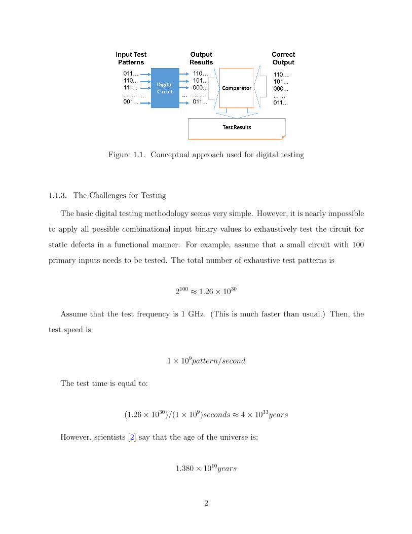
Figure 1.1. Conceptual approach used for digital testing

1.1.3. The Challenges for Testing

The basic digital testing methodology seems very simple. However, it is nearly impossible

to apply all possible combinational input binary values to exhaustively test the circuit for

static defects in a functional manner. For example, assume that a small circuit with 100

primary inputs needs to be tested. The total number of exhaustive test patterns is

2100 ≈ 1.26 × 1030

Assume that the test frequency is 1 GHz. (This is much faster than usual.) Then, the

test speed is:

1 × 109pattern/second

The test time is equal to:

(1.26 × 1030)/(1 × 109)seconds ≈ 4 × 1013years

However, scientists [2] say that the age of the universe is:

1.380 × 1010years

2

That means that exhaustively testing for a circuit of only 100 inputs with all possible

input requries 2900 times the age of our universe. Obviously, only a very small subset of all

possible test patterns can be applied. Therefore, to achieve high quality parts, an optimized

test set should detect the maximum number of defects with the available testing resources.

Unfortunately, even when they are created with signficant effort, test sets may not be

perfect, as shown in Figure 1.2. For example, because only a subset of all possible patterns

are applied, some of the defective circuits may pass testing and increase the customer’s risk

of buying bad chips. The fraction of all chips that are sold to customers but are actually

defective is called the defect level. At the same time, when circuit conditions during test

that do not match actual conditions in the field (or when non-logic based tests are applied)

may cause good circuits to fail the tests, leading to yield loss. Therefore, how to select the

test patterns for the test set and apply them in an appropriate way is a challenge for testing.

The increasing number of embedded instruments being inserted in the chip makes the

chip more complexity. Meanwhile, this embedded integration reduces the primary inputs

of the chip also challenged for testing. IEEE 1149 [1] and IEEE 1687 [3] standards have

been established. Based on these standards, there are the improvement have been proposed,

such as [85]. However, these standards have security risks. To resolved these risks, many

proposals have been published, such as [29,38,39].

Figure 1.2. Possible testing outcomes

3

1.2. Motivation

Generally, test sets for manufacturing defects attempt to detect them using at least one

of two basic strategies. When test sets are generated with automtatic test pattern generation

(ATPG) software, they usually model at least some of the defects as faults, target them, and

deterministically ensure that they are covered by the test set. The other primary approach

is probablistic. Much longer test sets are applied, and it is hoped that the defects will be

detected fortuitously.

Probabilistic approaches include both Logic Built-In-Self-Test (LBIST) with pseudo-

random or weighted psuedo-random patterns as well as approaches that attempt to maximize

the defect detection obtained with ATPG test sets. Examples include N-Detect [91], Gate-

Exhaustive Testing [24], and Embedded-Multi-Detect (EMD) [34]. However, these methods

are not efficient. Too many test patterns are used, and this often leads to memory issues

in automatic test equipment (ATE) when ATPG-based probabilistic approaches are to be

applied. This also signifcantly increases test time and test cost. Furthermore, some of the

defects require very specific detection conditions that are not usually met by the fortuitous

test patterns.

The alternative to probabilistic detection is to deterministically target specific faults that

are (hopefully) well-matched to the defects that actually occur. The most common fault

models are stuck-at faults, transition faults [94] and bridging faults [67]. Traditionally, all of

these fault models are based on the same assumption—that a fault only occurs at a library

cell’s input or output or the interconnect lines between the library cells. Unfortunately,

researchers have recently noted that those traditional fault test sets are not necessarily good

at detecting all of the real layout-based defects that occur inside standard cells [40].

To address this issue, in 2009, some researchers proposed the cell-aware fault model [40]

to explicitly represent and target library cell-internal defects. Cell-aware faults are obtained

from the detailed analog models that consider different types of defects that may occur in

the standard cell’s layout. The detection conditions are abstracted up to logic values at

the inputs of the standard cell that can be targeted during ATPG. Unfortunately, the test

4

set needed to achieve 100% cell-aware fault coverage often leads to a large increase in test

pattern count that can be commercially prohibitive. For example, a previously published

paper [41] showed that on average a 49% and 70% increase in test pattern count was needed

to achieve full cell-aware static and delay fault coverage when compared to full stuck-at and

transition fault detection, respectively on ten industrial circuits. Thus, a primary goal of

our research is to detect cell-aware faults efficiently with a smaller test set that reduces the

test time.

5

1.3. Main Contributions

This dissertation is composed of three main parts:

1. Preliminary Investigation: Exploration of the relationship between the detection re-

quirements of cell-aware and stuck-at faults and the characterization of cell-aware fault

detectability for standard cells from two digital standard cell libraries.

2. Development of a DFT-based Approach to Reduce Cell-Aware Test Pattern Count

through Scan Shift cCapture: Enhanced the detection capability of stuck-at test sets

for cell-aware static fault detection by using intermediate shift patterns.

3. Optimizations of the DFT Approach: reducing hardware overhead, reducing fault sim-

ulation time, and test set generation.

For the Preliminary Investigation:

• We generated a simple fault model, which we call the sub-gate-exhaustive fault model,

that can be used to investigate more stringent detection requirements than those needed

for stuck-at faults without requiring layout information or analog circuit analysis. For

each fault, we selected one of the possible input combinations at the inputs of the

standard cell and combined that input combination with the appropriate stuck-at fault

at the output. This defined the detection conditions for the sub-gate-exhaustive fault.

The fault could then be analyzed for its ability to be detected by various test sets.

• We explored the ability of different N-detect test sets to detect sub-gate-exhaustive

faults. We showed that some of these test sets are biased against detecting sub-gate-

exhaustive faults whose detection requirements prevent observation of upstream sig-

nals. In other words, an N-detect stuck-at test set may be unsuitable for detecting

some of these faults.

• We built on previous work that explored approaches to target test sets at those faults

that are most likely to be functional [90] and extended this analysis to sub-gate-

exhaustive faults. We peformed functional simulation of a good version of the circuit

6

and extracted flip-flop values on each clock cycle as a “good state.” We then refor-

matted these good states as test patterns that could be sent to a fault simulator to

determine which sub-gate-exhaustive faults were functional faults as opposed to poten-

tially non-functional. We then determined the number of top-off ATPG test patterns

needed to cover functional sub-gate-exhaustive faults missed by stuck-at test sets.

• We then began investigating true cell-aware faults. Our analysis showed that test sets

that detect all cell-aware faults in standard cells with more than two inputs are usually

much smaller than the corresponding gate exhaustive test sets for those cells. These

experimental results were obtained for both an academic standard cell library and a

commercial standard cell library. These results indicate that the gate exhaustive tests

may be overkill when trying to cover the defects inside the standard cell, and thus it

is worthwhile to analyze the layout and explicitly model the cell-aware faults.

• We investigated the ratio of care/don’t care bits in the test patterns generated to detect

all cell-aware faults in a single standard cell. Our experimental results showed that

generally the percentage of don’t care bits in the test sets targeting static or dynamic

cell-aware faults is much less than the corresponding percentage for test sets that

detect stuck-at or transition faults. This makes it more difficult to generate compact

cell-aware test sets in larger circuits comprised of multiple standard cells.

For the DFT Approach:

• We investigated a DFT design that allows us to harness scan shift cycles for proba-

bilistic fault detection. The approach involves inserting a Multiple Input Signature

Register (MISR) comprised of shadow flip-flops to collect a signature of the circuit

response while test values are being shifted into/out of the scan-chain. This allows

those intermediate shift patterns to serve as actual test patterns capable of testing for

cell-aware faults on each clock cycle.

• Our experimental results showed that, in most of the circuits studied, intermediate

shift patterns can cover 90% or more of the cell-aware faults that would otherwise be

missed by a stuck-at test set.

7

• This approach can also be used to fortuitously detect stuck-at faults and reduce stuck-

at fault test set size.

For the Optimizations:

• Because fault simulating all intermediate shift patterns for large circuits may be im-

practical, we investigated the effectiveness of capturing test data only on a subset of

regularly sampled intermediate shift patterns.

• We designed a MISR capture controller to enable capturing of shift cycle data to occur

at regular intervals. This reduces fault simulation time and/or reduces the need to tell

the tester hardware on which cycles capture should occur.

• We explored the ability to trade off the reduction of test patterns with the need to

meet low overhead requirements and achieved good results.

• To obtain a test-set agnostic method for selecting which flip-flops to shadow, we in-

vestigated an approach that uses the counts of the number of fault cones that pass

through a flip-flop.

• We investigated an approach that gradually generated test patterns with a heuristic

method to reduce redundant detection conditions.

8

Chapter 2

BACKGROUND

2.1. Functional vs. Structural Testing

2.1.1. Functional Test

To avoid the exhaustive testing mentioned in section 1.1.3, one of the obvious approaches

is to restrict the test to those input combinations that can occur in functional mode. If all

functional behavior is included in the test, then defects that would be missed by such a

test set can be considered harmless for the functional operation of the circuit. In fact,

detecting such faults could lead to unnecessary yield loss [81]. Such a test set used would

be equivalent to one used for brute-force complete design verification. However, while such

an approach may be better than a truly exhaustive test set, it is still extremely expensive

timewise whether used for test or design verification.

Furthermore, functional tests used for design verification are often not complete, and even

these incomplete tests are often much too long to be used for manufacturing test of every

device. Hence, a functional test set applied at manufacturing generally can include only a

limited subset of the functional test patterns. Such test sets are generally not considered

sufficient for acheiving high quality parts. Instead, structural tests must be applied as well.

2.1.2. Structural Test

In 1959, Eldred [32] proposed that tests should be generated by targeting the logical

structure of the circuit instead of its functional modes. In particular, because defects are

physical problems in the circuit structure, he proposed modeling the effect of such defects

on the logical operation of the circuit. A fault is a model of a defect. Faults can be targeted

9

deterministically by automatic test pattern generation (ATPG) software.

Structural test has many advantages, including the following:

• Structural test pattern generation does not require knowledge of the underlying func-

tional intent of the design and thus can be performed without designer expertise.

• Fault coverage (the percentage of all targeted faults detected by a test set) can serve

as a straightforward metric for test set quality. Even though this metric is not perfect

because modeled faults may differ from the actual defects, it allows us to compare test

sets and can provide a stopping point for ATPG.

• When appropriate DFT hardware, such as scan chains, are inserted into a design for

structural test, the controllability and observability of the circuit sites can be signifi-

cantly increased. The circuit can be placed in an arbitrary state, and even a sequential

circuit may be treated as combinational logic during ATPG.

• Structural tests generally achieve higher fault coverage than functional tests.

• Debug and diagnosis are often more efficient when structural tests are used because it

is easier to pinpoint the pattern that caused the failure.

However, while structural tests have many advantages, some defects that would be caught

by a limited set of functional tests may be missed by structural tests. For example, the

authors of [64] showed that 2% of the defective parts missed by purely structural tests for a

circuit were covered by functional test patterns. As a result, when high quality is desired, a

combination of structural and functional tests are often used.

2.2. Fault Models

Defects are physical problems in a manufactured copy of a chip that may prevent that

chip from operating correctly. In contrast, faults are models of defects that abstract the

behavior of a defect to its effect on the circuit’s logic. This effect can then be used to

generate test sets that target the modeled faults and deterministically detect them. When

faults are well-matched to defects, a test set that covers all of the faults will often cover all of

10

the defective circuits as well. Circuits that contain defects that were not covered during test

are known as test escapes, and to reduce the number of test escapes, multiple fault models

have been proposed: single stuck-at faults and multiple stuck-at faults, transition faults,

bridging faults, path delay faults, and cell-aware faults, among others.

2.2.1. Single Stuck-at Fault Model

The single stuck-at fault model assumes that a defective circuit site is permanently set

at either a logic 1 or logic 0. For example, this would occur if a circuit site were shorted

to either power or ground, respectively. Only a single site in the circuit is assumed to be

defective, where a circuit site corresponds to either an input or output of a logic gate. In the

case of a fanout connection, the branch is considered as a distinct site from the stem. Figure

2.1 is an example of a faulty circuit where a single stuck-at fault that occurs at a branch of

a fanout does not affect the other branch. More specifically the fault affects the input to the

XOR but does not affect the AND gate.

Two conditions must be satisfied to detect a fault or defect. First, the fault must be

excited. This means that the value at the faulty site must be different in the good and faulty

circuits. In Figure 2.1, exciting fault P stuck-at 0 requires setting site P to a logic 1 in

the good circuit to create this difference, and this value at P must be justified at a primary

input. Thus, exciting the fault requires setting input A to a logic 1.

The second requirement that must be satisfied is observation. This entails propagating

the value at the defective site to an observable output so that the fault effect can be seen. In

Figure 2.1, this means that the fault effect at site P must be propagated to the output Sum.

Note that because the site P is an input to an XOR gate, either value on the other XOR

gate input will allow propagation to occur. Thus, the value of B is X (i.e. ”don’t care”) and

here we have randomly selected the value of logic 1 to be used to replace the X.

Traditionally, the single fault model is the most widely used fault model for structural

test. Some of its advantages include the following:

• It is a structural fault model that allows ATPG to operate at the netlist level.

11

Figure 2.1. A half adder with a single stuck-at fault

• Because it is a static fault model, it is easily modeled, and fewer test patterns are

needed than for delay faults.

• The number of faults grows linearly with circuit size and is equal to 2n when the

number of sites in the circuit is equal n. This number can be further reduced with

fault equivalence and dominance relations. (Although it is possible to have more than

one defect in a circuit, circuits that contain mulitple defects are often easier to detect

and thus, the single fault assumption has shown itself to be a good assumption for

ATPG.)

• Well developed ATPG and fault simulation tools and algorithms are available.

• Some of the defects that do not perfectly match the stuck-at fault model are often

detected with tests that target stuck-at faults. For example, bridge faults are often

detected by stuck-at tests. This occurs because a test set targeting stuck-at faults

is required to observe every site in the circuit at least twice with different excitation

conditions. Further excitation requirements that need to be satisfied for more complex

defects can sometimes be met fortuitously during stuck-at fault detection.

2.2.2. Transition Fault Model

Static fault models, such as the stuck-at fault model, assume that a defect causes a

12

permanent change in the circuit’s function. However, some defects only insert additional

delay into the circuit. If one waits long enough, the circuit will provide the correct response.

However, if it does not provide a correct response in the required clock period, errors will

occur. To better model delay defects, various fault models have been proposed. The simplest

of these is the transition fault model.

There are two types of transition faults: slow-to-rise and slow-to-fall. Any site in a circuit

where a stuck-at fault can occur could contain a transition fault instead. Thus, as in the

case of stuck-at faults, the number of transition faults in the fault list grows linearly with

circuit size, and is equal to 2n for n circuit sites. The transition fault model also assumes

that the delay added by the fault is large, and thus transition faults may be detected even

along short paths with high slacks.

Because delay faults need to excite transitions in the circuit for the fault to be excited,

two-pattern tests are needed. For example, to detect site P slow-to-rise, the first pattern

must set site P to a logic 0, while the second pattern must set site P to a logic 1. This causes

the value at site P to “rise.” At the same time, the value of site P must be propagated to

an output during the second pattern to observe the fault.

2.2.3. Cell-aware Fault Model

Traditional fault models such as stuck-at and transition faults on place faults on the

interconnections between gates in the circuit. It is assumed that the interior of standard

cells are fault-free or that the faults modeled at the inputs and outputs can detect any

faults associated with the interior of those cells. However, this is not guaranteed. Thus,

as acceptable test escape rates have decreased to a few defective parts per million or less—

especially for critical applications such as automotive—some researchers have proposed the

cell-aware fault model [40,43–45,79] to explicilty target the defects inside the standard cells

and deterministically test for them.

Cell-aware faults are obtained by identifying all possible physical cell defects extracted

from the standard cell layout. Analog analysis is performed and detection conditions are

13

abstracted from analog level up to digital logic values at the inputs of the standard cell. The

detection conditions for a cell-aware fault can be listed as one or more combinations of logic

values at the inputs to the standard cell along with a corresponding stuck-at fault (for static

defects) or transition fault (for delay defects) at the cell’s output that must be propagated

to a circuit output for observation to occur.

Some important characteristics of the cell-aware fault model are:

• A test set with 100% cell-aware fault coverage targets more defects than a test set that

targets stuck-at and/or transition faults because stuck-at and transition faults are a

subset of a cell-aware fault list.

• Because this model abstracts the analog detection conditions of the defects up to digital

values at the inputs and outputs of the standard cell, ATPG algorithms can be used

to generate tests for them.

Unfortunately, because the cell-aware fault model introduces more faults with more strin-

gent detection conditions than traditional fault models, such as stuck-at and transition faults,

test sets that target cell-aware faults generally require more patterns, although they are sig-

nificantly shorter than gate-exhaustive patterns [45], [25]. For some industrial circuits, the

increase is large. For example, the authors of [41] performed experiments on 10 industrial cir-

cuits. They generated test sets that maximized the cell-aware fault coverage. They achieved

an average defect coverage gain of around 5% (1% static and 4% delay). However, the

number of static test patterns increased by 49% versus a stuck-at fault test set. For delay

patterns, the test set increased by 70%.

2.3. Test Set Generation

Generally, the methodology of test generation is classified into two categories: probabilistic

and deterministic.

14

2.3.1. Probabilistic

The probabilistic method is to maximize the fortuitous detection of untargeted (unmod-

eled) defects. In other words, we hope to detect the defects “through luck.” Well-known

techniques that include N-detect, Gate Exhaustive, and random test and LBIST.

2.3.1.1. N-detect

All faults and defects, regardless of type, must be both excited and observed for detec-

tion to occur. Excitation requirements vary from one type of fault/defect to another, but

observation of the site in error is a common requirement. Every time a site is observed, there

is a chance that defects at that site may be fortuitiously excited at the same time. Thus,

the more times a site is observed with different patterns, the higher the likelihood that all

defects at that site have been detected.

This observation leads to the n-detect approach for defect detection. In this approach,

every targeted fault is guaranteed to be detected at least n times, where n is generally

greater than one. Usually, the targeted faults are stuck-at faults, and an n-detect test set

that targets stuck-at faults guarantees that each circuit site is observed at least 2n times—n

times when that site is equal to a logic one and n times when that site is equal to a logic

zero. These tests have been shown to obtain good fortuitous detection of unmodeled faults

and defects (e.g. [15,31,37,62,75,76]).

Such test sets are easy to generate with standard ATPG tools. However, they are gener-

ally much longer than a standard test set. Furthermore, in some cases, an n-detect test that

tries to maximize n with as few patterns is possible can be biased against detecting defects

that block observation of upstream logic values, as will be discussed in Chapter 3.

2.3.1.2. Gate Exhaustive

Another probabilistic approach is Gate Exhaustive Testing [66]. In this approach, the

output of every m-input gate in the circuit is observed at least 2m times—once for each of

the 2m possible logic values for that gate. Such test sets use a brute-force approach to make

15

sure that static defects inside the gate are excited and observed. However, the resulting test

sets are often even longer than an n-detect test set unless n is very high. Such test sets for

single standard cells will be compared to cell-aware test sets later in the dissertation.

2.3.1.3. Random Test and Logic BIST

Random pattern generation had been used for testing in [12]. This technique is especially

appropriate for Built-In-Self-Test, where on-chip circuitry is used to generate pseudo-random

patterns to be applied to the Circuit Under Test (CUT). They are called pseudo-random

because, although they may have many characteristics of random patterns, the patterns

applied to the circuit can be predicted ahead of time based on knowledge of the circuit

generating them. Because the pseudo-random patterns to be applied are known ahead of

time, good circuit simulation can be used to predict the appropriate response. At a high

level, this architecture is shown in Figure 2.2.

Figure 2.2. BIST architecture in the high level

Generally, the pattern generator shown in 2.2 is a pseudo-random generator based on

a linear feedback shift register (LFSR). An LFSR consists of a series of flip-flops wired as

a shift-register with feedback at specific points through XOR gates. Figure 2.3 shows an

example of an LFSR. An LFSR can be specified using a characteristic polynomial equation.

The polynomial for the LFSR shown in Figure 2.3 is

16

Figure 2.3. LFSR with third degree polynomial

P (x) = 1 + x2 + x3 (2.1)

The maximum number of unique pseudo-random test patterns that can be generated by

an LFSR is

2n − 1 (2.2)

where n is the number of flip-flops in the LFSR. This corresponds to all possible combi-

nations of n bits except for the combination that corresponds to all 0s. (If all 0s are placed

in the flip-flops of an LFSR, then the LFSR’s state cannot change.) The LFSR shown in

Figure 2.3 can generate up to 23 − 1 = 7 unique test patterns. They are:

100, 010, 101, 110, 111, 011, 001

The response analyzer for LBIST is usually implemented with a multiple input signature

register (MISR). The function of a MISR is to combine and compress several output streams

into a single signature. The value the MISR should contain at the end of testing can be

determined based upon good circuit simulation. However, if defects are present in the circuit

and the error propagates to the MISR, the signature will generally be different from that of

the good circuit. This allows the defect to be detected when the actual signature is compared

to the expected signature.

17

Figure 2.4. Multiple Input Signature Register (MISR)

However, there is still the low possibility that a fault signature is identical to the fault-free

one. This is called MISR aliasing. In this situation, the fault will escape the test. To resolve

this problem, we can change the connections of XORs by using an different characterisic

polynomial, change the seed for starting the MISR, or add additional flip-flops and make a

larger MISR.

The capability of pseudo-random patterns to detect faults is highly dependent on circuit

characteristics. Circuits that are highly observable and controllable may have many “easy-

to-detect” faults and be very random-pattern testable. Other circuits may have sites that

are much more difficult to observe and control and be much less amenable to this approach.

Weighted random patterns and test points have both been proposed to increase the fault

coverage during LBIST [22, 46]. Alternatively, top-off ATPG patterns can be applied to

detect those faults that are not covered by LBIST.

LBIST is particularly useful when tests are applied in the field. However, the overhead,

power consumption, and costs of the added logic gates are increasing. Furthermore, the chip

yield may actually decrease due to defects in the LBIST circuitry. Therefore, the feasiblity

of using LBIST for a circuit must be evaluated based on the cost-benefit analysis.

18

2.3.2. Deterministic

The deterministic method targets the modeled faults directly, and generates a test set

to detect them. Fault models were discussed in Section 2.2. Here we further explain test

generation.

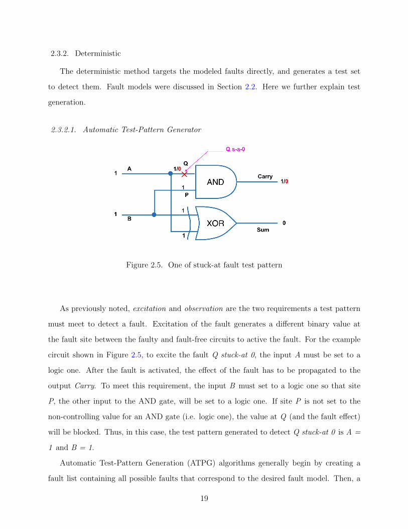
2.3.2.1. Automatic Test-Pattern Generator

Figure 2.5. One of stuck-at fault test pattern

As previously noted, excitation and observation are the two requirements a test pattern

must meet to detect a fault. Excitation of the fault generates a different binary value at

the fault site between the faulty and fault-free circuits to active the fault. For the example

circuit shown in Figure 2.5, to excite the fault Q stuck-at 0, the input A must be set to a

logic one. After the fault is activated, the effect of the fault has to be propagated to the

output Carry. To meet this requirement, the input B must set to a logic one so that site

P, the other input to the AND gate, will be set to a logic one. If site P is not set to the

non-controlling value for an AND gate (i.e. logic one), the value at Q (and the fault effect)

will be blocked. Thus, in this case, the test pattern generated to detect Q stuck-at 0 is A =

1 and B = 1.

Automatic Test-Pattern Generation (ATPG) algorithms generally begin by creating a

fault list containing all possible faults that correspond to the desired fault model. Then, a

19

fault is selected for targeting, and a pattern is generated. If dynamic compaction is used, and

if sufficient “don’t care” values are present in the generated pattern, then other faults can

be targeted, and new assignments to the primary inputs can be made to try to detect them

with the same pattern. Two of the earliest ATPG algorithms were the D-Algorithm [82]

and PODEM [36]. Over the years, a variety of optimizations and additional algorithms have

been proposed to reduce the time required to run ATPG and generate more efficient and

compact test sets.

2.3.2.2. Fault Cones

One of the optimizations used to make ATPG more efficient has been the use of fault

cones. Through a forward trace of a circuit’s topology starting at a fault site, some of parts

of the circuit can be reached. Those parts are reachable are called the fault cone [19]. Figure

2.6 illustrates this concept. Consider two possible stuck-at faults: A stuck-at 0 and P stuck-

at 1. Starting at fault A stuck-at 0 and tracing the circuit’s topology toward the outputs,

we find that gates G1, G2, G3, and the output Y are downstream. Therefore, G1, G2, G3,

and Y compose the fault cone of fault A stuck-at 0 and are marked in blue. Similarly, G5,

G6, and Z are in the fault cone of fault P stuck-at 1 and are marked in orange. .

Fault cones have been used during ATPG to analyze which circuit sites can possibly be

affected by a fault [71]. Some papers have also proposed analyzing fault cones to insert test

points [96–98].

2.3.2.3. Scan-Chain

ATPG for sequential circuits is much more difficult than for combinational circuits be-

cause sequential circuits cannot be placed immediately in an arbitrary state, and some circuit

sites cannot propagate their values immediately to a circuit output. More specifically, justi-

fying values in the circuit interior to the circuit’s primary inputs may first require justifying

values to the circuit’s flip-flops (or other state holding elements) and then further justify-

ing those flip-flop values to the inputs over one or more previous clock cycles. In addition,

20

Figure 2.6. Faults and fault cones

Figure 2.7. Scan chain

21

propagation of a fault to a flip-flop does not make it immediately observable. If a fault can

only be propagated to a flip-flop in the current clock cycle, then that flip-flop value must

be propagated to the primary outputs in a subsequent clock cycle. Thus, sequential ATPG

requires analysis of the circuit over many time cycles. This is difficult and inefficient, and

the fault coverage achieved is often low.

To address this problem, scan chains have been devised to aid in ATPG by allowing

circuits to be considered as combinational logic during ATPG. They do this by modifying

the circuit to allow an arbitrary state to be shifted into the circuit’s flip-flops and allow

values that have been captured in the flip-flops to be shifted out.

The high-level structure of a circuit containing a scan chain is shown Figure 2.7. This

figure shows a the standard Huffman model for a sequential circuit, in which combinational

logic uses the current input values and current state held in the flip-flops to calculate the

current output and next state values that will be clocked into the flip-flops on the next clock

edge. When a scan chain architecture is used, each flip-flop in the circuit is replaced with a

scan flip-flop that allows it to be concatenated into a large shift register that can be used to

shift patterns into and out of the flip-flops from Scan in to Scan out during test.

Figure 2.8. Scan flip-flop

Scan chain insertion generally involves replacing each flip-flop in the design with a MUX-

D Scan flip-flop, such as that shown in Figure 2.8 [19]. The scan flop consists of a flip-flop

and a multiplexer (MUX). By controlling the scan enable (SE) signal, we can determine

22

whether the value clocked into the flip-flop is coming from the previous bit on the chain (SI

for Shift In) or from the circuit’s combinational logic (D).

During test, each test pattern is first shifted into the scan chain from scan in. For a

chain of length n, this takes n clock cycles. Next, the circuit is placed in functional mode

by changing the value of SE. The clock is pulsed, and data from the circuit is captured in

the flop flops. Then the circuit is once again placed in shift mode, and the test results are

shifted out at the same time that the next pattern is shifted in. The values shifted out can

then be compared to the expected values.

23

Chapter 3

FUNCTIONAL VS. NONFUNCTIONAL FAULT DETECTION

As discussed in Chapter 2, ATPG-generated structural tests have many advantages over

functional patterns. The fault coverage of these structural patterns is generally high and easy

to quantify, and many well-known algorithms are available to generate them. They are also

often an easier choice for debugging and diagnosis. However, traditional structural patterns

can still miss many defects if they are generated by targeting faults that don’t match the

defects that actually occur. One possible solution is to target additional fault models to

capture a wider variety of defect behavior. The cell-aware fault model is one such model.

In Chapter 2, we also discussed probabilistic approaches to defect detection. Instead

of explicitly modeling different types of defects, these ATPG methods aim to enhance the

chances of fortuitously detecting the unmodeled defects. The most common probabilistic

approach is n-detect, where the ATPG tool tries to detect each targeted fault at least n

times, where n is generally greater than one. In fact, ATPG tools, such as Mentor GraphicsTM

Tessent [6], allow one to specify not only the number of guaranteed fault detections, but also

the number of desired fault detections. This allows the corresponding test set to attempt to

maximize the number of fault detections without significantly affecting the pattern count.

Thus, a reasonable question to ask is whether these various optimized tests are capable

of fortuitously detecting faults that have more stringent conditions to satsify at the inputs to

a standard cell than a normal stuck-at fault. Such requirements are related to those needed

for cell-aware fault detection. We explore this question by investigating the detection of

“sub-gate-exhaustive” faults and how they interact with the optimization techniques used

for n-detect.

24

In this chapter1, we define a sub-gate-exhaustive fault by selecting one of the possible

input combinations of a standard cell combined with a stuck-at fault at the output of the

corresponding standard cell. Then, we use Mentor GraphicsTM Tessent to generate multiple

probabilistic n-detect test sets with different values of n and evaluate each test set for its

ability to detect sub-gate-exhaustive faults. We determine which sub-gate-exhaustive faults

are missed by the probabilistic approaches and show why an n-detect test set may actually

be biased against their detection. We then explore how many top-off patterns would be

needed to detect the missed sub-gate-exhaustive faults and how functional evaluation of

their criticality can potentially reduce the number of patterns that need to be applied.

Thus, we aim to determine whether it is possible to use a combination of a probabilistic and

deterministic approaches in concert with functional analysis to create effective and efficient

test sets for these types of faults..

3.1. Sub-Gate-Exhaustive Faults And Their Relation To Stuck-at ATPG

Usually, to make ATPG easier, the detection conditions for defects are abstracted to

logical values at the inputs of the cells. A standard cell with n inputs has 2n possible input

combinations. We define a sub-gate-exhaustive fault as a fault whose detection requires

exactly one of these input combinations to be placed at the inputs to the cell while the

appropriate stuck-at fault is observed at the output of the standard cell. Of these input

combinations, some subset may be needed for 100% stuck-at fault coverage of the cell, but

not all. For example, consider Figure. 3.1.

This figure shows a simple AND gate and the four possible input combinations for that

AND gate. The second input combination in the list is required to detect A stuck-at-1

because it is the only input combination that both excites the stuck-at-1 fault and allows its

value to propagate through the gate to the output. Similarly, the third input combination

is required to detect B stuck-at-1 while the last input combination is required to detect A

stuck-at-0, B stuck-at-0, and F stuck-at-0.

1This chapter is based on a previously published paper [92].

25

Figure 3.1. Mandatory and non-mandatory input combinations for full stuck-at fault cov-

erage.

Only the first input combination, with both inputs equal to zero, is not required for the

detection of any fault. It does not allow either of the two input signals to be propagated

through the gate and observed. If all the sub-gate-exhaustive faults in our fault list for this

AND gate required one of the final three input combinations for detection, then all of them

would be guaranteed to be detected by a stuck-at fault test set. Only when a sub-gate-

exhaustive fault list required the 00 input combination would the ATPG tool need to be

“lucky to obtain full sub-gate-exhaustive fault coverage.

In general, for all AND, OR, NAND, and NOR gates of n inputs, the number of input

combinations required for full stuck-at fault coverage is equal to n + 1. This corresponds to

setting all inputs to the non-controlling value for one input combination, as well as setting all

inputs but one to the non-controlling value, iterated over each input, for n additional input

combinations. In the case of XOR and XNOR gates, no input combination is mandatory

because there is no controlling value. In general, as the number of inputs to the gate

increases, the percentage of input combinations that are not required for full stuck-at fault

26

coverage increases as well. Other potential standard cells, such as multiplexers and AOI

(and-or-invert) cells also have multiple input combinations that are not required for full

single stuck-at fault coverage, although they could be a part of a stuck-at fault test set.

3.1.1. The Reasoning Behind N-detect Test Sets

At least in full-scan circuits, ATPG tools are generally capable of creating test sets with

very high stuck-at fault coverage. However, a problem often arises due to the presence of

defects that are not well-modeled by the targeted faults, and this leads to test escapes.

There are two primary requirements for the detection of any fault or defect: excitation

and observation. Defect excitation corresponds to creating a difference in logic value at the

defect site between a good and defective circuit. In the case of a stuck-at fault, this simply

requires setting the logic value at the defect site to the non-stuck value. In the case of a

bridge fault, it requires setting the value of the two ends of the bridge to opposite values. In

the case of a sub-gate-exhaustive faults, it may require a particular combination of values at

the inputs of a standard cell. Obviously, these requirements vary from one type of fault or

defect to another.

In contrast, site observation is a common requirement among all types of defects. No

matter what type of defect occurs or what its excitation requirements are, the incorrect logic

value must be propagated to an observation point (output or flip-flop on the scan chain) for

the defect to be detected.

Thus, in the past, we have shown that the reason why n-detect test sets improve defect

detection is because they increase the number of observations of circuit sites [31]. Each

additional stuck-at fault detection at a site provides another opportunity for fortuitously

exciting an unknown defect. Of course, to ensure that these additional observations are

valuable, the resulting patterns must be sufficiently different from each other. For example,

previous research has shown that increasing the probability that circuit sites are balanced

with respect to their excitation values [28], and considering the values in a particular region

around a gate in the layout [27] can improve the defect coverage of n-detect test sets. Also

27

note that the impact of each additional detection of a fault is greater when there are fewer

detections of that fault so far. The second detection is more valuable than the third, and

the third detection is more valuable than the fourth. In fact, we have shown previously that

the ability of another stuck-at fault detection to detect an as yet undetected defect (such as

a bridging defect) decreases exponentially as the number of previous detections of that fault

increases (e.g. [30,88,89]).

As a result, of this, one might expect that increasing the value of n when n is currently

very small would provide a good opportunity to increase the detection of sub-gate-exhaustive

faults while at the same time also detecting other types of untargeted faults. Thus, improved

sub-gate-exhaustive faults coverage might be free. However, there is a potential contradiction

between the requirements for achieving the maximum number of stuck-at fault detections and

obtaining high sub-gate-exhaustive faults coverage. Specifically, for many gates, those input

combinations to a cell that are not mandatory for 100% stuck-at fault coverage are exactly

those that prevent the inputs of the cell from being observed. Thus, choosing patterns that

maximize the number of stuck-at fault detections could be biased against the detection of

at least some sub-gate-exhaustive faults. To investigate this, we ran experiments on several

different types of n-detect test sets.

3.1.2. Experiments for Sub-Gate-Exhaustive Fault Detection by N -detect Test Patterns

Our preliminary investigations were performed on several of the largest ISCAS 89 bench-

mark circuits: s38584, s38417, s15850, s13207 and s9234 [18]. Because we are interested in

those input combinations on logic gates that may be required for the detection of a sub-

gate-exhaustive faults and yet are not guaranteed to be detected by a test set with 100%

stuck-at fault coverage, we selected a subset of these input combinations combined with

the appropriate stuck-at fault at the ouput of the corresponding standard cell as our ”sub-

gate-exhuastive” fault, and added them to the fault list as separate faults. To ensure that

the results were not highly dependent on the particular input combinations selected, two

different fault lists were created for each circuit.

28

Specifically, each fault set differed in the input combinations required for sub-gate-

exhuastive detection for all gates with more than 2 inputs. (Two input gates that are

not XOR or XNOR have only one input combination that is not required for 100% stuck-at

fault detection.) Thus, for example, in one fault set the input combination required for a

sub-gate-exhuastive fault detection on a four input AND gate might be 0101, while in the

other fault set it could be 0010. Each fault list was implemented with the User Defined

Fault Model option in Mentor GraphicsTM Tessent, and fault simulation was performed for

stuck-at fault ATPG test sets created with four different n-detect test set strategies:

• n0 (disable multiple detection function)

• n1 (guaranteed detections=1, desired detections=3)



In this case, the n1 test set is most similar to the embedded n-detect test set used in [40]

because additional detections are added to a single-detect test set with minimal increase (if

any) in pattern count. Which sub-gate-exhuastive faults in each fault list were detected by

each test set was recorded, and the total number of sub-gate-exhuastive faults detected in

each case is shown in Table 3.1. Those faults that were not detected by the corresponding

n-detect test set were subsequently targeted with sub-gate-exhuastive ATPG. The total

number of test patterns in each test set, including the sub-gate-exhuastive top-off patterns,

is shown in Figures 3.2 and 3.3, with the total height of the bar corresponding to the total

length of the combined test set. (For now, ignore the reference to“good state set 1” as this

refers to functional simulations that will be described shortly.)

At this point, we are only interested in the number of test patterns allocated to each test

set for sub-gate-exhaustive fault detection vs. stuck-at fault detection. The orange and blue

portions of each bar correspond to top-off patterns generated separately for full detection

of the non-redundant sub-gate-exhaustive faults in the fault list, while the cream colored

29

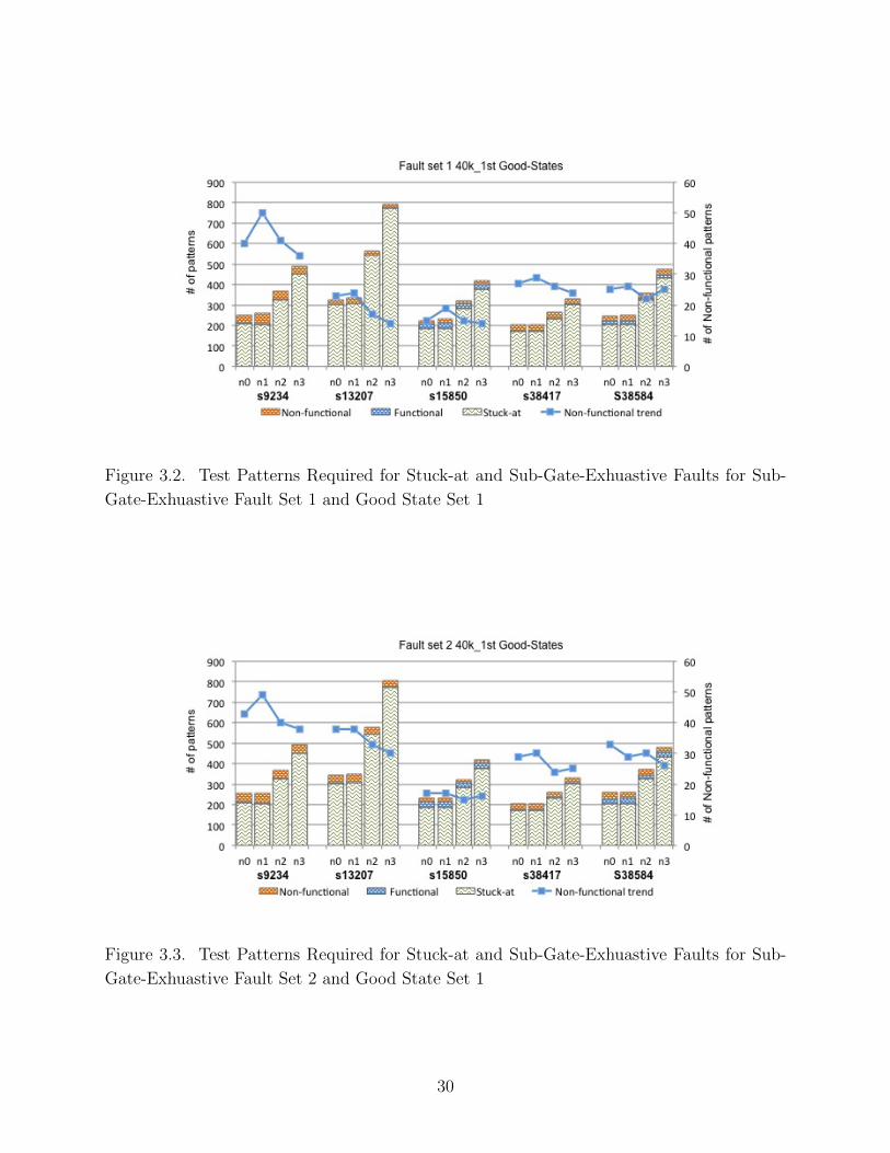
Figure 3.2. Test Patterns Required for Stuck-at and Sub-Gate-Exhuastive Faults for Sub-

Gate-Exhuastive Fault Set 1 and Good State Set 1



30

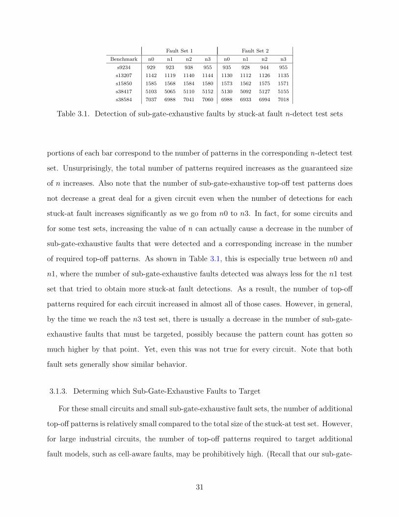
Fault Set 1 Fault Set 2

Benchmark n0 n1 n2 n3 n0 n1 n2 n3

s9234 929 923 938 955 935 928 944 955

s13207 1142 1119 1140 1144 1130 1112 1126 1135

s15850 1585 1568 1584 1580 1573 1562 1575 1571

s38417 5103 5065 5110 5152 5130 5092 5127 5155

s38584 7037 6988 7041 7060 6988 6933 6994 7018

Table 3.1. Detection of sub-gate-exhaustive faults by stuck-at fault n-detect test sets

portions of each bar correspond to the number of patterns in the corresponding n-detect test

set. Unsurprisingly, the total number of patterns required increases as the guaranteed size

of n increases. Also note that the number of sub-gate-exhaustive top-off test patterns does

not decrease a great deal for a given circuit even when the number of detections for each

stuck-at fault increases significantly as we go from n0 to n3. In fact, for some circuits and

for some test sets, increasing the value of n can actually cause a decrease in the number of

sub-gate-exhaustive faults that were detected and a corresponding increase in the number

of required top-off patterns. As shown in Table 3.1, this is especially true between n0 and

n1, where the number of sub-gate-exhaustive faults detected was always less for the n1 test

set that tried to obtain more stuck-at fault detections. As a result, the number of top-off

patterns required for each circuit increased in almost all of those cases. However, in general,

by the time we reach the n3 test set, there is usually a decrease in the number of sub-gate-

exhaustive faults that must be targeted, possibly because the pattern count has gotten so

much higher by that point. Yet, even this was not true for every circuit. Note that both

fault sets generally show similar behavior.

3.1.3. Determing which Sub-Gate-Exhaustive Faults to Target

For these small circuits and small sub-gate-exhaustive fault sets, the number of additional

top-off patterns is relatively small compared to the total size of the stuck-at test set. However,

for large industrial circuits, the number of top-off patterns required to target additional

fault models, such as cell-aware faults, may be prohibitively high. (Recall that our sub-gate-

31

exhaustive faults are intended to correspond to one set of detection conditions that may be

needed for a potential cell-aware fault.) In addition, even when the number of additional

patterns seems to be small overall, if those additional patterns require a re-load of tester

memory, even a small number of extra patterns may be prohibitively expensive. As a result,

we also looked at which sub-gate-exhaustive faults should be targeted if we cannot target all

of them.

Recall that one of the reasons to add sub-gate-exhaustive faults to our ATPG process at

all is to reduce the number of test escapes and subsequent field returns. Thus, intuitively, it

makes sense that those sub-gate-exhaustive faults that are more important from a functional

perspective, and thus most likely to lead to field returns, should be targeted first. The

realization that some faults are more important than others is not a new idea. In [81],

Rearick noted that detecting non-functional timing defects could unnecessarily lower yields.

Other researchers have even deemed that known defective parts can be sold if it is unlikely

that the end user will ever use the product in such a way that the defects present will affect

them (e.g. [16, 17, 52, 60]). The authors of [48] intentionally modify test sets to minimize

the detection of acceptable faults so that they cannot cause failures and reduce yields. The

authors of [49] ran test patterns to determine how defective a chip actually was for product

grading purposes.

While we do not necessarily advocate selling parts known to be defective or avoiding

fault detections to increase yields, in the past, we have also optimized stuck-at fault test sets

for fault criticality, which we considered to be a function of the number of times a fault on

a given clock cycle would cause an error that could ultimately propagate to an output seen

by the end user [89], [88], [87]. We were able to show that detecting more critical stuck-at

faults could lead to detecting more critical untargeted surrogate defects. In the current work,

we harness this idea, but instead of trying to fortuitously detect more critical untargeted

defects with our stuck-at fault test patterns, we instead investigate the ratio of how many

sub-gate-exhaustive faults appear to really be functionally important as opposed to those

that have not yet been shown to be detectable.

32

Figure 3.4. Overall flow for determining which sub-gate-exhaustive faults are functionally

important for one set of sub-gate-exhaustive faults and one-set-of good states. This flow is

repeated four times: for two fault lists and two sets of good states.

The overall flow of the experimental procedure is shown in Figure 3.4. First, we create

our two sub-gate-exhaustive fault lists for each circuit as described in Section 3.1.2. At the

same time, we use SynopsysTM VCS [9] to generate good-state patterns. For our purposes,

good state patterns correspond to circuit states (inputs and flip-flop values) that were seen

during normal sequential simulation of a design. Unfortunately, we do not know the real

applications for these benchmark circuits, and thus, our input sequences are random. (We

are assuming that these random sequences are representative of field operation.) In these

experiments, we run two different test sets of 40,000 patterns each for each circuit to obtain

two sets of good circuit states for each circuit.

Next, we insert a scan chain into each benchmark circuit for use during ATPG and

fault simulation. We then create three different types of test sets for the evaluation of

sub-gate-exhaustive detection characteristics. First, we perform stuck-at fault ATPG using

Mentor GraphicsTM Tessent [6] for the four types of n-detection test sets listed in Section

3.1.2. These are our baseline test sets that we assume would be applied regardless of their

detection of sub-gate-exhaustive faults. We also take our good circuit states extracted from

33

sequential simulation and place them in a format that can be used by Tessent to perform

fault simulation. Finally, we also run ATPG on our sub-gate-exhaustive faults using the

UDFM option in Mentor GraphicsTM Tessent. This allows us to determine which of these

sub-gate-exhaustive faults are redundant (or tied) and can be ignored.

Both the stuck-at ATPG test sets and the good state patterns are then fault simulated

for our sub-gate-exhaustive faults to determine which non-redundant sub-gate-exhaustive

faults are detected by each set of patterns. Simulation of the ATPG test sets allows us

to determine which of our sub-gate-exhaustive faults were not fortuitously detected by each

stuck-at n-detect test set. In contrast, the fault simulation of our good state patterns for sub-

gate-exhaustive faults is used to determine which sub-gate-exhaustive faults were detected

by the good state patterns and thus are assumed to be functionally relevant. Faults that have

been shown to be functionally relevant should be targeted before potentially non-functional

faults when the number of test patterns that can be applied is limited.

Note that in these experiments, we are assuming that if a fault reaches a flip-flop or a true

output on a single good state cycle that it is indeed detected. Of course, there is a possibility

that an error that reaches a flip-flop in the first cycle may subsequently be masked and never

reach a true output. Also note that just because a fault is not detected during good-state

simulation does not mean that it is guaranteed to be non-functional. In fact, faults with

very low detection probability relative to the number of patterns applied may show up as

functional for one set of random patterns and not another, and we saw this happen in rare

cases. Other faults with lower detection probabilities may not show up at all. As a result,

it is important to remember that these faults are only potentially non-functional.

Thus, for each circuit studied and for each n-detect test set, we obtain one list of functional

sub-gate-exhaustive faults that were not detected by the n-detect test set and one list of

potentially non-functional sub-gate-exhaustive faults that were not detected by the n-detect

test set for four different cases:

• Good State Set 1, Cell-Aware Fault Set 1


34



Keeping the functional and potentially non-functional faults separated allows us to gen-

erate the top-off patterns for them separately. The simulation results of these experiments

for the first set of good state patterns are shown in Figures 3.2 and 3.3. The results for the

second set of good state patterns are shown below in Figures 3.5 and 3.6.



In these figures we can see that varying the good state test sets and the fault lists did not

significantly change the results. In each graph, the blue portion of each bar corresponds to

top-off patterns needed to detect sub-gate-exhaustive faults that were detected at least once

during the good state simulation (i.e. would have caused an error to occur and propagate

to an output or flip-flop during normal sequential simulation.) The orange bars correspond

to the top-off patterns needed for sub-gate-exhaustive faults that were never seen to cause

a failure in the corresponding good state simulation. In each of the four graphs, there

are generally more top-off patterns needed to test for potentially non-functional sub-gate-

35



exhaustive faults than those that test for functional sub-gate-exhaustive faults. The blue

lines on each figure correspond to the y-axis on the right side of each graph and show how

many patterns are being added to detect potentially non-functional faults. Once again, it is

clear that simply increasing the number of guaranteed and desired detects during stuck-at

ATPG does not necessarily reduce the number of additional patterns that are being added for

what may very well be functionally redundant faults. This is especially true as we move from

n0 to n1, although it can also happen between n1 and n2 and between n2 and n3. Yet, the

overall trend is that the total number of patterns added for potentially non-functional sub-

gate-exhaustive fault detections appears to decrease significantly from n0 to n3. However,

the number of patterns added may still be significant. The percentage increase in test length

is shown in Figures 3.7 through 3.10.

These graphs represent the total percent increase in pattern count corresponding to

patterns that test for potentially non-functional faults and were added as top-off patterns

compared to the number of tests for stuck-at ATPG plus top-off patterns needed to test for

known functionally relevant sub-gate-exhaustive faults. Here again we see that two different

36

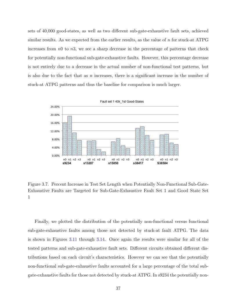
sets of 40,000 good-states, as well as two different sub-gate-exhaustive fault sets, achieved

similar results. As we expected from the earlier results, as the value of n for stuck-at ATPG

increases from n0 to n3, we see a sharp decrease in the percentage of patterns that check

for potentially non-functional sub-gate-exhaustive faults. However, this percentage decrease

is not entirely due to a decrease in the actual number of non-functional test patterns, but

is also due to the fact that as n increases, there is a significant increase in the number of

stuck-at ATPG patterns and thus the baseline for comparison is much larger.

Figure 3.7. Percent Increase in Test Set Length when Potentially Non-Functional Sub-Gate-

Exhaustive Faults are Targeted for Sub-Gate-Exhaustive Fault Set 1 and Good State Set

1

Finally, we plotted the distribution of the potentially non-functional versus functional

sub-gate-exhaustive faults among those not detected by stuck-at fault ATPG. The data

is shown in Figures 3.11 through 3.14. Once again the results were similar for all of the

tested patterns and sub-gate-exhaustive fault sets. Different circuits obtained different dis-

tributions based on each circuit’s characteristics. However we can see that the potentially

non-functional sub-gate-exhaustive faults accounted for a large percentage of the total sub-

gate-exhaustive faults for those not detected by stuck-at ATPG. In s9234 the potentially non-

37



1



2

38

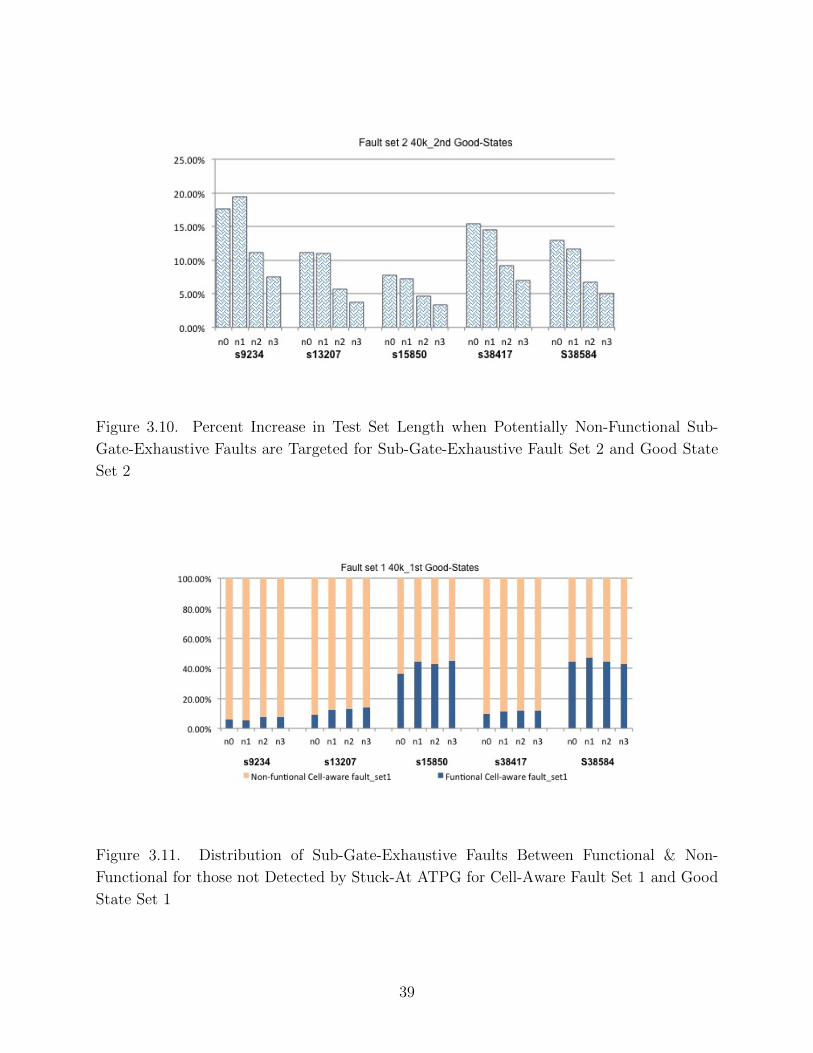
Figure 3.10. Percent Increase in Test Set Length when Potentially Non-Functional Sub-

Gate-Exhaustive Faults are Targeted for Sub-Gate-Exhaustive Fault Set 2 and Good State

Set 2

Figure 3.11. Distribution of Sub-Gate-Exhaustive Faults Between Functional & Non-

Functional for those not Detected by Stuck-At ATPG for Cell-Aware Fault Set 1 and Good

State Set 1

39



State Set 1



State Set 2

40



State Set 2

functional sub-gate-exhaustive faults accounted for 90-94% of all the sub-gate-exhaustive

faults that were not detected by stuck-at ATPG. Even in s38584, the potentially non-

functional sub-gate-exhaustive faults accounted for 50-56% of the total sub-gate-exhaustive

faults that were not detected by stuck-at ATPG. Finally, there does not seem to be a clear

trend in the data as the test sets go from n0 to n3.

3.2. Summary

In this chapter we have described an investigation of the relationship between the detec-

tion of sub-gate-exhaustive faults and test sets optimized for n-detect. Overall, the exact

trends may vary from one circuit to another, but in general, even the large increases in

pattern count that occur with the n3 test sets do not necessarily yield a corresponding in-

crease in sub-gate-exhaustive fault detection. In some cases the gain in sub-gate-exhaustive

coverage is negligible. Furthermore, when the number of desired detections increases, but

the pattern count does not change significantly (as occurs when going from n0 to n1), the

number of detected sub-gate-exhaustive faults may actually decrease. This is not a flaw in

41

the ATPG tool or n-detect algorithm. It is due to a fundamental tension between the fact

that some sub-gate-exhaustive fault detection conditions may require us to reduce circuit

site observations while maximizing the number of stuck-at fault detections requires us to

increase circuit site observations. Thus, other options may be needed to reduce the impact

of sub-gate-exhaustive faults on the overall test set size when testing resources are limited.

One way to do this is through the analysis of which of the sub-gate-exhaustive faults are

truly capable of (or more likely to) cause functional failures. These faults should be targeted

first, and our experiments have shown that some sub-gate-exhaustive faults do appear to

be more likely to cause errors in functional mode. These experiments were performed using

limited simulation of good circuit states. However, while such simulation may show that

faults are functional, it does not prove that undetected faults are non-functional. Thus, Fur-

ther analysis may be needed if it is necessary to prove that faults are truly non-functional

before they are not targeted during test. Such analysis may be necessary for highly critical

applications with very high quality requirements.

42

Chapter 4

CHARACTERIZATION OF CELL-AWARE FAULT DETECTABILITY

This chapter expands the previous analysis of sub-gate-exhaustive faults to encompass

both true cell-aware fault and gate exhaustive fault models. In particular, it explores how a

subset of all possible input combinations for a standard cell can be used as a compact test

set that will detect all of the internal cell-aware faults identified through layout and analog

based analysis of a single standard cell in the NanGate Open Cell Library [7] or a commercial

library. One goal is to determine the underlying character of the cell-aware faults and verify

why they lead to larger tests sets. Another goal is to determine how close the single cell test

set is to the set of gate exhaustive patterns for that cell.

4.1. Background

In Chapter 3, we investigated ways in which various input combinations that may be

needed for the detection of internal faults could be detected (or not) by n-detect test sets.

We showed that some input combinations for various gates are “n-detect resistant,” and any

cell-aware faults that require those combinations for detection may actually be more likely to

be missed when the number of “guaranteed” and “desired” detections are increased without

a corresponding increase in pattern count.

However, at the time that data was collected, we did not have access to actual cell-aware

faults that were identified through analog analysis of faults inserted into the layout. Instead,

we had to select a subset of all input combinations as our “sub-gate-exhaustive faults.” Later,

we found and began analyzing the NanGate FreePDK45 Generic Open Cell Library [8] and

began investigating the characterization of static and dynamic (i.e. delay-based) cell-aware

faults.

43

The NanGate FreePDK45 Generic Open Cell Library [8] is a generic open source 45 nm

library that was created for research purposes by the Silicon Integration Intiative. According

to their website, it was generated using Nangate’s Library Creator TM [7] and North Carolina

State University’s FreePDK Base Kit [4]. Characterization was performed using Arizona

State’s Predictive Technology Model (PTM). Because it was intended only for research, the

library was generated using non-optimized Open PDK and cannot be used for the actual

manufacture of integrated circuits. However, this library is compatible with the commercial

cell-aware fault generation tool we used that automates the analysis of standard cell libraries

for potential defects, and thus it allows us to generate a cell-aware fault list for each circuit.

Later, our experiments were also repeated using standard cells from a commercial standard

cell library.

4.2. Extracting Layout-Based Cell-Aware-Type Faults from Cell-Aware ATPG

of Standard Cells

In this portion of the project, we focused on standard cells operating as individual circuits

so that we could characterize the test patterns needed to achieve 100% fault coverage of the

standard cell when traditional fault models were used as opposed to the cell-aware fault

model. More specifically, we wanted to explore how many patterns layout-based cell-aware

faults required when compared to the normal stuck-at and transition patterns that would

need to be applied to achieve 100% coverage of those other types of faults. In particular, the

goal here was to see how many additional patterns are really necessary for detecting cell-

aware faults when compared to both stuck-at and transition faults when no other constraints

arising from other gates in the circuit are involved. (In a larger circuit, more patterns may be

needed if these particular input combinations conflict with required logic value assignments

on other gates/standard cells. On the other hand, faults for multiple standard cells in a

larger circuit may be detectable with a single pattern.) We also wanted to determine how

similar these “best case” pattern counts are to not only stuck-at and transition faults, but

also to gate exhaustive faults. Thus, we also ran ATPG for stuck-at and transition faults on

44

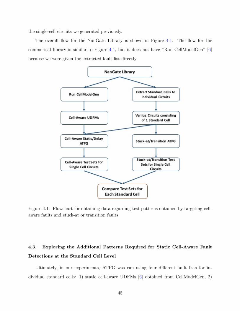
the single-cell circuits we generated previously.

The overall flow for the NanGate Library is shown in Figure 4.1. The flow for the

commerical library is similar to Figure 4.1, but it does not have “Run CellModelGen” [6]

because we were given the extracted fault list directly.

Figure 4.1. Flowchart for obtaining data regarding test patterns obtained by targeting cell-

aware faults and stuck-at or transition faults

4.3. Exploring the Additional Patterns Required for Static Cell-Aware Fault

Detections at the Standard Cell Level

Ultimately, in our experiments, ATPG was run using four different fault lists for in-

dividual standard cells: 1) static cell-aware UDFMs [6] obtained from CellModelGen, 2)

45

dynamic/delay-based cell-aware UDFMs created with CellModelGen, 3) stuck-at faults, and

4) transition faults. Each type of experiment was implemented using standard cells from

the NanGate library and from the commerical library. We were primarily interested in the

pattern count for each resulting test set. Gate exhaustive test set sizes depend only on the

number of gate inputs and do not require ATPG. Once test sets were obtained for each fault

list, we considered static and dynamic faults separately. Figures 4.2, 4.3, 4.4, 4.5 and 4.6

show the corresponding data for static faults.

Figure 4.2. Comparison between the number of test patterns required for compressed test

sets covering different types static faults for NanGateTM library

Figure 4.2 shows the number of test patterns in the stuck-at (red line) and cell-aware

(green line) test sets for each of the 96 standard cells in the NanGateTM library. The standard

cells are sorted on the x-axis in increasing number of inputs (1 to 6) as well as in increasing

number of stuck-at fault test patterns. The blue line shows the number of patterns that

would be needed for each standard cell for gate exhaustive testing.

As would be expected, as the number of inputs increases, the number of patterns needed

to achieve 100% fault coverage of the standard cell increases as well. In the case of both

46

the stuck-at and cell-aware faults, the number of patterns needed is actually quite similar

and usually much lower than the number of test patterns needed for gate exhaustive testing,

indicating that gate exhaustive tests are probably not needed to obtain good cell-aware fault

coverage for defects within the standard cell and that a layout-based analysis is worthwhile.

Figure 4.3. Comparison between the number of test patterns required for compressed test

sets covering different types of static faults for the commercial library

The results shown in Figure 4.3 have been collected from standard cells in the commer-

cial library. It has almost 2500 cells and is much larger than the NanGateTMlibrary. The

collection and formatting of the data is similar to that shown in Figure 4.2. Once again, gate

exhaustive testing appears to be much more expensive than what is necessary for stuck-at

and cell-aware faults, especially for those cells with a high number inputs. Thus, layout

based analysis for fault extraction is important if compact test sets are desired.

To more clearly show the differences in pattern counts between stuck-at and cell-aware

faults for the commercial library standard cells, Figure 4.4 shows a “zoomed-in” version of

the data without the gate exhaustive pattern counts. The result is quite similar to Figure

4.2. The test set size required for cell-aware faults is usually bigger than stuck at faults for

47

Figure 4.4. Comparison between the number of test patterns required for compressed test sets

covering different types static faults without gate exhuastive pattern counts for commercial

library

each standard cell.

Figure 4.5 shows related data for the NanGateTM library, but in this case, the percent in-

crease in the number of patterns required for full stuck-at coverage vs.̃full cell-aware coverage

is shown as calculated with the formula:

Percent increase =] cell-aware patterns − ] stuck-at patterns

] stuck-at patterns× 100% (4.1)

Clearly, for some standard cells, there is a significant percent increase in the number of

patterns required. Generally, this is due to the presence of more complex standard cells. For

example, the increases in pattern count for the three-input gates 50-52 correspond to MUX

and Full Adder cells. Another increase at gate 58 is due to the OAI21 X4 gate.

Figure 4.6 shows similar data for the commercial library. However, the magnitude of the

increase is often larger than that shown in Figure 4.5. For example, some of the 3-inputs

cells require an almost 300% increase. We believe that this is due to characteristics of the

48

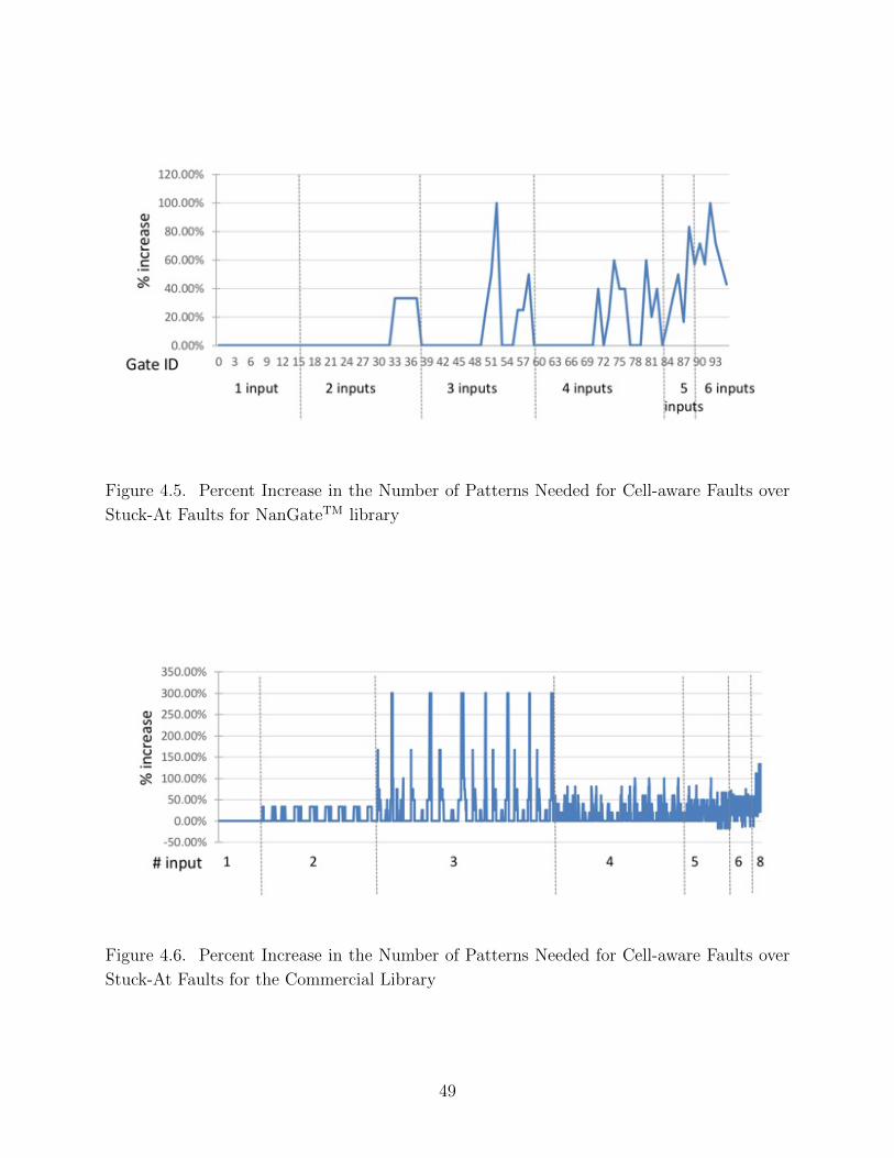
Figure 4.5. Percent Increase in the Number of Patterns Needed for Cell-aware Faults over

Stuck-At Faults for NanGateTM library

Figure 4.6. Percent Increase in the Number of Patterns Needed for Cell-aware Faults over

Stuck-At Faults for the Commercial Library

49

standard cells in the library.

Also note that for some of the standard cells with 5, 6, and 8 inputs, the number of

patterns required for cell-aware fault coverage is less than that required for stuck-at faults.

We believe that this may be due to random decisions made during ATPG during test pattern

generation.

Finally, we investigated the number of don’t care bits in the test patterns of the two

test sets for both stuck-at and static cell-aware faults. The results based on the NanGateTM

library are shown in Figure 4.7. The number of X’s is important because having more X’s in

the patterns means that these input combinations are likely to be more easily satisfied when

the faults are targeted in a larger circuit where compatible values must be found among

multiple gates on each test pattern. In Figure 4.7, we can see that the percentage of X’s in

the test patterns is very low for those standard cells that have few inputs. The percentage of

X’s increases for some standard cells with 3, 4, 5, or 6 inputs; however, in general, stuck-at

fault test patterns have more X’s than cell-aware. This is expected because internal cell-

aware faults that are not detected by stuck-at are likely to have more conditions that must

be satisfied for detection to occur. In fact, in most cases, the cell-aware test patterns have

no X’s at all.

The same experiment for comparing the number of don’t care bits in the test patterns

was also performed on standard cells from the commercial library. The results are similar to

those obtained from the NanGateTM library and are shown in Figure 4.8. When the number

of inputs to the standard cell is three or more, there are often significantly more X’s in the

stuck-at patterns than in the cell-aware patterns.

50

Figure 4.7. Average percentage of X’s in a test pattern for NanGateTM library

Figure 4.8. Average percentage of X’s in a test pattern for the commercial library

51

4.4. Exploring the Additional Patterns Required for Delay-Based Cell-Aware

Fault Detections at the Standard Cell Level

Similar data was also obtained for delay faults. Figures 4.9, 4.10, 4.11, 4.12, 4.13, 4.14,

4.15, and 4.16 show data for transition faults and delay-based cell-aware faults.

Figure 4.9. Comparison between the number of test pattern pairs required for compressed

test sets covering different types dynamic faults with gate exhuastive patterns for NanGateTM

library

We see the same trends in this data as in the static case, but they are often more

pronounced. More pattern pairs were required for cell-aware delay fault coverage than for

the transition fault coverage beginning with two-input cells. This increase occurs earlier

and remains more pronounced than the corresponding increase in the cell-aware static and

stuck-at pattern graph. The percentage of X’s in the pattern pairs is also much larger in the

case of transition faults than in the case of cell-aware faults.

4.5. Summary and Next Work

In this chapter, we have investigated the relationship between both delay-based and static

cell-aware faults and their corresponding traditional faults. We have found that the number

52

Figure 4.10. Comparison between the number of test pattern pairs required for com-

pressed test sets covering different types dynamic faults without gate exhuastive patterns

for NanGateTM library


test sets covering different types dynamic faults with gate exhuastive patterns for commercial

library

53


test sets covering different types dynamic faults without gate exhuastive patterns for com-

mercial library

Figure 4.13. Percent Increase in the Number of Pattern Pairs Needed for Cell-aware Faults

over Transition Faults for NanGateTM library

54

Figure 4.14. Percent Increase in the Number of Pattern Pairs Needed for Cell-aware Faults

over Transition Faults for commercial library

Figure 4.15. Average percentage of Xs in a test pattern pair for NanGateTM library

55

Figure 4.16. Average percentage of Xs in a test pattern pair for commercial library

of patterns needed to detect all cell-aware faults for a standard cell is much less than the

number of gate exhaustive test patterns. In addition, for less complex standard cells (such

as standard logic gates), the number of patterns required for both stuck-at and cell-aware

fault detection is often identical. It is primarily for more complex or high-input gates that

the difference between the two becomes pronounced, and a layout-based analysis becomes

necessary. In addition, the percentage of X’s in the cell-aware fault patterns is much less

than the percentage of X’s in the corresponding stuck-at or transition patterns. This has

the potential to make the detection of multiple cell-aware faults with a single pattern much

harder to do in larger circuits made up of many standard cells and helps to further explain

the increase in pattern count seen by many researchers for cell-aware test sets.

As previously noted, restricting fault targeting to only truly functional faults in a circuit

has the potential to make test sets more efficient. However, identifying which faults are

truly functional can be difficult. Thus, an alternative approach involves the use of enhanced

Design for Testability (DFT) circuitry to detect more cell-aware faults with an efficient test

set. The next chapter will investigate such an approach for the detection of cell-aware faults.

56

Chapter 5

PUTTING WASTED CLOCK CYCLES TO USE: ENHANCING FORTUITOUS

CELL-AWARE FAULT DETECTION WITH SCAN SHIFT CAPTURE

In Chapter 4, we investigated various aspects of the detectability of cell-aware faults

when only a single standard cell was present. The experimental results showed that even

for a single standard cell, the number of patterns required to detect all cell-aware faults was

often considerably larger than that required to detect all traditional (stuck-at or transition)

faults. Futhermore, the resulting test sets had fewer don’t care values in the patterns. As

a result, there are more opportunities for conflicts between the detection requirements of

various cell-aware faults, likely requiring separate patterns to detect each of them.

The authors of [11] have proposed adding control test points to appropriate locations in

the circuit where these conflicts may occur—allowing fanout branches to be set to different

values and reducing the number of cell-aware faults that cannot be detected together due to

either excitation or observation incompatibilities. ATPG tools must then take advantage of

those new controllability points to try to detect as many cell-aware faults with each pattern

as possible.

In this chapter2, we take a different approach. Instead of adding controllability test

points to try to make otherwise incompatible faults compatible, we aim to detect cell-aware

faults using only a stuck-at fault test set that has been generated normally. We consider the

fact that generally, when tests are applied to circuits that contain scan chains, test results

are only captured once the entire pattern has been shifted in and the desired deterministic

pattern has been applied. Intervening shift cycles serve only as overhead. This is done

because capturing data in the circuit’s scan flip-flops during scan shift would destroy the

pattern being shifted in. However, if data is captured in shadow flops in a MISR instead,

2This chapter is based on a previously published paper [93]

57

those shift cycles could be used to obtain additional fault coverage.

Thus, in this chapter, we investigate the ability of the intervening shift cycles to achieve

high static cell-aware fault coverage using only the test patterns generated to detect stuck-at

faults. We also investigate reducing the number of shadow flops required. Our results show

that high cell-aware coverage is achievable even when only a stuck-at test set is applied—in

some cases equal to the coverage obtained by a dedicated cell-aware test set.

5.1. Background and Related Work

As previously noted, an alternative probabilistic approach to detecting defects with

ATPG test patterns involves using an Linear Feedback Shift Register (LFSR) or another

pseudo-random pattern generator to apply a large number of patterns to the circuit dur-

ing Logic Built-In Self Test (LBIST) (e.g. [10, 20, 21, 26, 51, 56, 59, 101]). Often, test results

are captured as a signature using a Multiple Input Signature Register (MISR) that can be

compared against an expected signature.

Both test-per-scan and test-per-clock approaches have been proposed for LBIST. Test-

per-scan approaches use scan chains to shift the entire pseudo-random pattern into a circuit-

under-test before the test is applied, whereas test-per-clock approaches feed the outputs of

the test pattern generator to the circuit under test on each clock and collect the results from

the outputs of the circuit under test with a signature analyzer [19, 57, 58, 73]. For example,

the authors of [73] suggest a BIST scheme in which all flip-flops in the circuit are shadowed

to capture responses in a test-per-clock mode. The shadowed data is then combined with

the circuit output data in a separate MISR structure. Test patterns to detect stuck-at faults

are optimized for this structure and stored in an on-chip memory. In this chapter, we will

consider a related scheme with lower overhead that focuses on the fortuitous detection of

cell-aware faults in the presence of on-chip decompressors.

Other recent work describes a method that uses a test-per-clock approach and adds a

multiplexer and XOR gate to every flip-flop in the design so that different chains may be in

one of three modes during test: stimulus, compaction, or mission mode [69]. Compaction

58

mode utilizes the XORs to obtain a signature for selected chains. Stimulus mode involves

shifting, and mission mode simply allows that chain’s flip-flops to operate in normal mode.

Scan path stitching is changed to collect flip-flops into chains amenable to the approach, and

simulated annealing is used to determine which chain should be in each mode. Specialized

ATPG is used to create the test patterns. The authors of [80] also consider a pattern

generation and application approach that may shift data less than the full amount before

capturing data in flops without a MISR.

Because some faults are difficult to detect with random patterns, weights may be used

to bias the inputs in favor of a logic 0 or logic 1 to help increase the detection capability

(e.g. [23, 59, 100]). However, top-off patterns created with ATPG or deterministic BIST

are often still required to achieve acceptably high coverage for even single stuck-at faults

(e.g. [13], [47]).

5.2. Capturing Test Results on Scan Shift

Traditional scan-based test requires that a significant amount of time be spent shifting

data into and out of the scan chains. In fact, if the longest scan chain is of length L, then

at least L clock cycles are needed to shift the pattern into the chain. This is followed by at

least one cycle in normal mode to capture the values generated by the circuit in response to

the applied pattern (i.e. perform the test). This is then followed by at least an additional L

clock cycles required to shift the resulting data out. Of course, it is standard to overlap the

shifting in of one pattern with the shifting out of the following pattern. However, in general,

only one clock cycle out of every L+1 cycles is actually used for defect detection. This is

one reason why on-chip decompressors are often added to circuits, so that a long chain can

be broken up into many shorter scan chains that can be shifted simultaneously, if desired.

Intuitively, it seems that it should be possible to use the intervening shift cycles for defect

detection, but standard scan chain design makes this difficult or impossible if all chains are

going to be shifted simultaneously. In particular, if data were to be captured in the chains

on the intervening shift cycles, the captured data would destroy whatever pattern we were

59

attempting to shift into the chain, as shown in Figure 5.1.

This figure shows the standard Huffman model for sequential circuits with the state-

holding flip-flops connected together into a scan chain. Assume that we intend to shift the

pattern 0111 into the chain, starting with 0. If we capture data in the flops after the first

three bits have been shifted into the chain, then the contents of the chain will correspond

to the captured values, not the 011 that have been shifted in already. Thus, for example,

if the circuit generates a logic 0 on the bottom flop when X011 is currently present in the

chain, then the last bit will be set to 0 before the next shift if we capture first. Similarly, in

this figure, the second flop from the top will be set to a logic 1 before the next shift. The

end result is that the data that appears in the scan chain at the end of scan chain shifting

is 1101 instead of the 0111 that was intended.

Figure 5.1. Capturing data during scan shift will destroy the pattern being shifted into the

circuit.

60

Using the captured data for intervening shift cycles as part of the pattern is possible

(and to some extent is already done when applying launch on last shift or launch on capture

delay patterns at the very end of the scan shift process to apply delay patterns). However, as

in [80], this would make ATPG more complex if data were captured many times in the middle

of the scan shift sequence. The difficulty would likely be even higher for large numbers of

hard-to-detect cell-aware faults.

To avoid this increase in ATPG complexity and possible loss of coverage, we consider that

scan shift cycles can be harnessed for fortuitous cell-aware defect detection if a small amount

of additional DFT circuitry is added to the design to enhance its testability. In particular,

we explore how selected circuit sites can be augmented with observation test points that can

be collected into a MISR [70] that will capture data on the intervening scan shift cycles,

allowing each partially shifted in pattern to serve as an actual test pattern that can detect

cell-aware defects, as shown in Figure 5.2.

Figure 5.2. Sequential circuit in which selected scan flip-flops are shadowed in a MISR so

that a signature can be collected using intermediate shift data as test patterns

Thus, with this approach, we have the opportunity to augment the original deterministic

test set by increasing the number of effective patterns applied by up to a factor of L. When

61

one considers that a standard industrial circuit may contain scan chains with hundreds of

thousands of flip-flops, the potential impact on probabilistic defect detection with no increase

in test time is highly significant.

In the rest of this chapter, we will explore how this approach can improve the detectability

of cell-aware faults with a test set that was generated to target only stuck-at faults. We

will show that for most of the circuits studied, a large portion of the cell-aware faults are

fortuitously detected with a small number of scan shift patterns. We will explore the number

of scan flip-flops that need to be shadowed, the number of clock cycles on which the MISR

must capture data, as well as the possibility of aliasing in the MISR. Furthermore, we will

show that even the stuck-at test set size may be reduced with very little effort if the scan

shift patterns are used to detect stuck-at faults as well. This is all accomplished in the

presence of an on-chip decompressor.

5.3. Experimental Setup

Our experimental analysis was performed on five different circuits from opencores.org [5]

and one industrial circuit. The characteristics of these circuits are shown in Table 5.1. The

OpenCoresTM circuits were synthesized using the NanGate FreePDK45TM Generic Open

Cell Library [8], a standard cell library that contains the layout of each standard cell. As

discussed in the previous chapter, although the library was intentionally designed so that

it cannot be used to manufacture circuits, it was intended to allow challenges regarding

advanced technology nodes to be explored. This library is compatible with the commercial

cell-aware fault generation tool we used that automates the analysis of standard cell libraries

for potential defects, and thus it allows us to generate a cell-aware fault list for each circuit.

We also performed experiments on an industrial size circuit, Circuit A, that was synthe-

sized with a commercial library. All circuits shown in this paper were implemented with

on-chip decompressors. The sizes of the fault lists in the presence of on-chip decompressors

for each circuit are shown in Table 5.1.

62

compression

ratioffs

#stuck-at

faults

#cell-aware

faults

quadratic 2 120 ∼8200 ∼34500

des56 4 193 ∼13800 ∼54000

fm receive 9 501 ∼20000 ∼79000

colorconv 9 584 ∼38500 ∼184000

fpu double 27 5231 ∼297000 ∼1210000

circuit A 57 30462 ∼1263000 ∼5143000

Table 5.1. Circuit Charactierstics

The original cell-aware fault list created for each circuit contained both detectable and

non-detectable cell-aware faults. To determine how many faults were actually detectable, we

followed the overall procedure shown in Figure 5.3. We first ran cell-aware-ATPG and fault

simulation to see how many faults could be detected and to determine how many patterns

were required in a cell-aware test set for each circuit. We also ran normal stuck-at fault

ATPG to generate a stuck-at fault test set for each circuit. We then used a commercial tool

to perform cell-aware fault simulation on the stuck-at test set to determine which cell-aware

faults were missed by stuck-at fault ATPG. Finally, we extracted a test set that consisted of

all the intermediate shift patterns that would be seen by the circuit during scan-shift when

the stuck- at test pattern set was shifted through the chain. This test set of intermediate shift

patterns could then be fault simulated to determine its cell-aware fault detection capabilities

and identify how many additional detections of cell-aware faults were possible compared to

those detected by just the original stuck-at fault test patterns.

5.3.1. Defining Intermediate Shift Patterns

The procedure for defining the intermediate shift patterns is shown in Figure 5.4. We

assume that the flip-flops are reset to contain all 0’s before the first pattern begins to be

shifted in. This is necessary to avoid capturing X’s in the MISR. Alternatively, the MISR

could be set to not capture anything while the first pattern was being shifted in.

63

Figure 5.3. Procedure for identifying detectable cell-aware faults

64

Figure 5.4. Example of disassembling original test patterns into multiple intermediate test

patterns

65

Assume that the length of the scan chain is n. We then create n-1 intermediate test

patterns for pattern 1 that consist of the pattern iteratively being shifted in. They are

denoted as pattern 1_1, pattern 1_2, etc. Finally, on the nth shift, the 1st ATPG pattern

is entirely present in the scan chain. This is the pattern that will be applied, and the

corresponding test results will be captured in the normal scan chain (as opposed to just the

shadow flops/MISR). Thus, once the values are captured, the state of the chain corresponds

to the values that we expect to be scanned out from the chain due to pattern 1’s application

to the circuit under test. This capture pattern is shown with the dashed lines in the figure.

Next, pattern 2 starts to be shifted into the chain. Its intermediate scan patterns are a

combination of the capture values from pattern 1 as well as the ATPG-created values that

correspond to pattern 2. This process repeats until we have n*m partial patterns (including

the original ATPG patterns), where m is the number of patterns in the stuck-at test set,

and n is the maximum number of flip-flops in the chain.

5.3.2. Handling Chains of Different Lengths

When chains of different lengths are present in a circuit, the ATPG tool may pad the

test patterns for the shorter chains with X’s so that X’s are shifted into the short chains

before the actual values for the pattern are shifted in. For these experiments, those X’s were

replaced with randomly filled values of 1’ s and 0’s.

5.3.3. Handling X’s in Capture Values

In our experiments, only one of the circuits generated X’s in any of the capture values.

Fortunately, these X’s appeared only at the end of the test set (i.e. in the last several

patterns) as opposed to most patterns. We simply disabled the MISR (prevented it from

capturing any data) when any X’s would have been present in an intermediate shift pattern.

In other industrial circuits, more X’s may be present throughout the test set. Such X’s

could be handled with previously proposed techniques used for LBIST. Ways to optimize

the handling of X’s for the approach described in this chapter is part of our future work.

66

5.4. Experimental Results

5.4.1. Fortuitous Cell-Aware Fault Detectionby Intermediate Scan Shift Patterns

Our initial experiments tried to determine what percentage of the detectable cell-aware

faults that would have been missed by simply applying traditional stuck-at fault test pat-

terns could be detected by the same stuck-at fault test patterns if data were captured on

intermediate scan shift cycles as well as at the end of scan shift. In each case, all X’s in the

test patterns were filled with a standard random-fill procedure and the requirements of the

on-chip decompressor. The fault detection results can be seen in Figure 5.5.

Figure 5.5. Percentage of cell-aware faults missed by stuck-at ATPG patterns that are

detected when intermediate shift patterns are used for fault detection.

The overall detection percentages are generally very high. In all but one case, 90% or

more of the cell-aware faults that would have been missed were detected fortuitously with

scan shift intermediate patterns. For two circuits, all of the missed cell-aware faults were

detected. FPU has the lowest percentage of faults covered. We believe that this is due to

67

the character of the circuit. For example, the circuit likely has a large number of difficult-

to-observe sites. In future work, we will investigate ways of increasing coverage for this kind

of circuit by possibly changing observation points to be in alternative locations and by more

intelligent filling of X’s in the test patterns.

5.4.2. Test Set Size Reduction

Because we decided to apply the entire stuck-at fault test set regardless of the number of

stuck-at faults that might have been detected fortuitously by the intermediate patterns, the

reduction in pattern count for patterns to be stored is limited by the difference between the

test set that was generated by targeting cell-aware faults and the test set that was generated

by targeting stuck-at faults.

Of course, as shown in the previous section, for some circuits we were still not able to

obtain 100% cell-aware coverage through fortuitous detection in the intermediate pattern

test set. If we still want to detect those faults, one approach is to generate top-off patterns

for them with ATPG. Alternately, it may be possible to modify the tests (e.g. by adding

more constraints or intelligently filling X’s to achieve better coverage with the original test

pattern set. The test set size compared to the cell-aware-test set when the stuck-at test set

or the stuck-at test set with top-off patterns are used can be seen in Figure 5.6.

In this figure, the percentage of patterns required varies between 45% and 80% of the orig-

inal cell-aware test set when top-off patterns are not used to get the remaining coverage for

all of the cell-aware faults. (Lower numbers are better.) When top-off patterns are applied,

the pattern counts vary between approximately 55% and 90% of the original. Note that in

each case, the original test set was generated for a circuit with an on-chip decompressor.

Also note that the overall reduction is ultimately limited by the size of the original stuck-at

test set, which we kept intact. Finally, note that even reducing the overall pattern count

by 10% can correspond to significant savings when the total number of original patterns is

large.

68

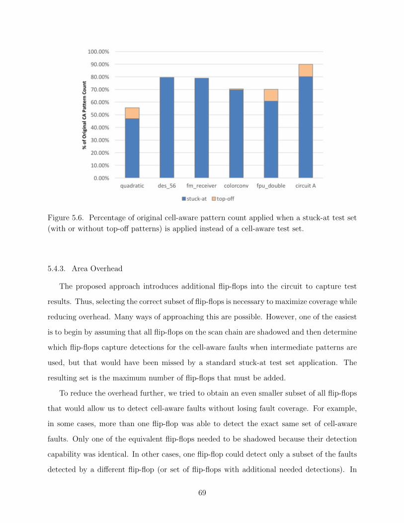
Figure 5.6. Percentage of original cell-aware pattern count applied when a stuck-at test set

(with or without top-off patterns) is applied instead of a cell-aware test set.

5.4.3. Area Overhead

The proposed approach introduces additional flip-flops into the circuit to capture test

results. Thus, selecting the correct subset of flip-flops is necessary to maximize coverage while

reducing overhead. Many ways of approaching this are possible. However, one of the easiest

is to begin by assuming that all flip-flops on the scan chain are shadowed and then determine

which flip-flops capture detections for the cell-aware faults when intermediate patterns are

used, but that would have been missed by a standard stuck-at test set application. The

resulting set is the maximum number of flip-flops that must be added.

To reduce the overhead further, we tried to obtain an even smaller subset of all flip-flops

that would allow us to detect cell-aware faults without losing fault coverage. For example,

in some cases, more than one flip-flop was able to detect the exact same set of cell-aware

faults. Only one of the equivalent flip-flops needed to be shadowed because their detection

capability was identical. In other cases, one flip-flop could detect only a subset of the faults

detected by a different flip-flop (or set of flip-flops with additional needed detections). In

69

that case, only the flip-flops that detected a greater number of faults (e.g. the dominating

flip-flops) would need to be shadowed. Following these rules, we identified a set of flip-flops

that could be used to detect all cell-aware faults that were detectable by the intermediate

shift patterns. Figure 5.7 shows a flow-chart depicting this optimization procedure.

Figure 5.7. Flip-Flop Selection Procedure for Inclusion in the MISR

The overhead results are shown in Figure 5.8. This figure shows the percentage of the

original flip-flops that were included in the MISR. The subset of flip-flops selected for the

first five circuits (i.e. the OpenCoresTM circuits) was identified using the algorithm described

in Figure 5.7. Due to time constraints, the overhead for Circuit A contains all flip-flops that

can detect any of the cell-aware faults missed by normal stuck-at fault ATPG. The additional

procedure shown in Figure 5.7 was not applied. In all cases, the circuits contained an on-chip

decompressor, and the data going into the actual scan chains in the devices was used to do

fault simulation.

70

Figure 5.8. Percentage of original circuit flip-flops that were included in a set of flip-flops

capable of detecting all detectable cell-aware faults in the circuit.

The maximum percentage of flops that needed to be shadowed varied from approximately

1.8% for fm rev to 41.67% for quad, the smallest circuit. The largest circuit, circuit A,

required approximately 10.23% of all scan flip-flops to be shadowed.

Note that even further reductions in the area overhead are likely possible. For example,

we could reduce the number of flip-flops required by XORing multiple values to compact

them into one shadow flop as long as the same fault cannot propagate along multiple paths

into the XOR. Other less greedy algorithms could also be applied to help cover all fault

detections with an even smaller number of flops.

5.4.4. Intermediate Shift Cycles Needed for Capture

In general, the number of intermediate shift patterns available for fault detection is very

large because it is proportional to the number of flip-flops on the chain. So, in the case of fpu,

we have the equivalent of over 470,000 patterns available. Of these, only a very small fraction

is needed to detect the remaining cell-aware faults. If our main goal is to only achieve high

71

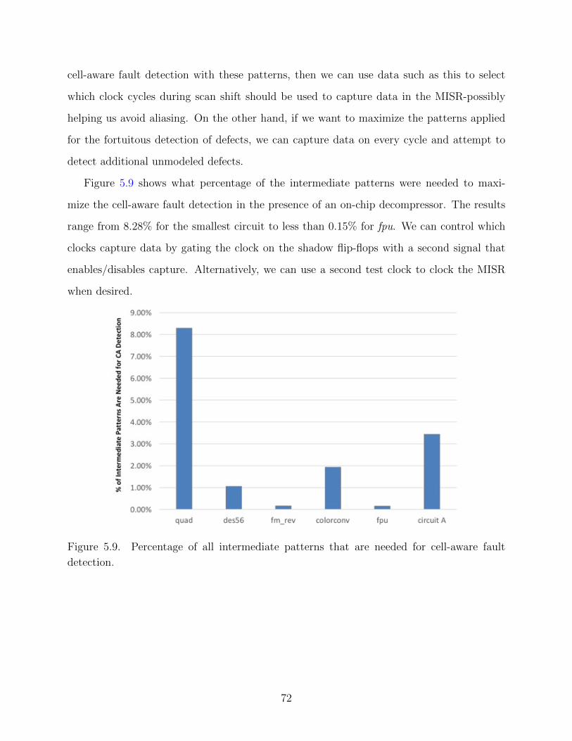
cell-aware fault detection with these patterns, then we can use data such as this to select

which clock cycles during scan shift should be used to capture data in the MISR-possibly

helping us avoid aliasing. On the other hand, if we want to maximize the patterns applied

for the fortuitous detection of defects, we can capture data on every cycle and attempt to

detect additional unmodeled defects.

Figure 5.9 shows what percentage of the intermediate patterns were needed to maxi-

mize the cell-aware fault detection in the presence of an on-chip decompressor. The results

range from 8.28% for the smallest circuit to less than 0.15% for fpu. We can control which

clocks capture data by gating the clock on the shadow flip-flops with a second signal that

enables/disables capture. Alternatively, we can use a second test clock to clock the MISR

when desired.

Figure 5.9. Percentage of all intermediate patterns that are needed for cell-aware fault

detection.

72

5.4.5. MISR Aliasing

Once we know which clock cycles and flip-flops that will be used to capture data into the

MISR, we can investigate the possibility of aliasing. To explore this, we need to identify the

fault-free MISR signature through simulation and then fault simulate each of the targeted

cell-aware faults to find the corresponding faulty signature. Due to time constraints, only

the OpenCoresTM circuits were simulated for aliasing effects. The results are shown in Table

5.2 for the OpenCoresTM circuits.

Clearly, the number of fault detections missed due to aliasing in the MISR is tiny, and

in some cases zero. Although we were not able to obtain this data on Circuit A, we believe

that the results will likely be similar. Note that some of this aliasing could be reduced by

adding a few flip-flops to the MISR or otherwise changing the MISR design.

5.4.6. Reducing the Stuck-at Fault Test Set

All of our experiments so far have assumed that the original stuck-at fault test set will

be applied regardless of which stuck-at faults may be detected using the intermediate scan

shift patterns. However, just as it is possible to fortuitously detect cell-aware faults with

intermediate shift patterns, it is possible to fortuitously detect stuck-at faults with those

patterns as well. In fact, it is likely to be even easier because stuck-at faults are generally

easier to excite than the related cell-aware faults.

Circuit Flip-flops in MISR # Faults Missed

quadratic 50 0

des56 65 3

fm receive 9 2

colorconv 81 0

fpu double 305 1

Table 5.2. MISR Aliasing

73

To get an initial estimate for how much the stuck-at test set itself could be reduced, we

took a very greedy approach. Specifically, the intermediate patterns were fault simulated

for stuck-at faults. The number of new stuck-at faults detected by each pattern (both the

ATPG-generated pattern and the intermediate patterns seen during scan-in) was recorded.

Unfortunately, all patterns with zero new stuck-at fault detections could not necessarily

be removed from the test set. This is because the intermediate patterns applied depend

on both the pattern being shifted in as well as the captured values from the pattern being

shifted out. For example, consider Figure 5.10.

Figure 5.10. Example demonstrating interaction between adjacent patterns.

In this figure, the values already in the chain while the new pattern j is being shifted

in are shown as Ci. They correspond to the values captured in the chain(s) when pattern i

was applied. The new values for pattern j are shown as J ′s. They fill the chain so that the

74

intermediate patterns are a combination of the Ci and J values. Finally, pattern J has been

entirely shifted into the chain, the test pattern is applied, and the results are captured as

Cj. The Cj patterns are then shifted out as pattern K is shifted in.

Thus, the usefulness of pattern J is dependent on both its interaction with the previous

patterns capture values and the subsequent patterns shift in values. If no new faults are

detected while pattern J is being shifted in, but if new faults are detected when pattern K is

being shifted in while J ′s capture values are being shifted out, it isnt safe to remove pattern

J without performing more analysis. To avoid this additional analysis, we were very greedy

in our approach and only removed a pattern from the stuck-at fault test set if both that

pattern and the pattern after it achieved no new fault detections. Thus, for every string of

patterns that do not detect new stuck-at faults, we leave one of them (the last one) in the

test set. Note that this removal of patterns is only possible because the ATPG tool resets the

on-chip decompressor after every pattern is applied to place the decompressor in a known

state that is not dependent on the previous pattern.

Finally, it is well known that often the test patterns that are generated late in the ATPG

process are more effective for detecting hard faults. They are generated to target the difficult

faults that were not fortuitously detected earlier in the ATPG process. In addition, they

may be able to detect not only the hard faults they target, but also easier faults that were

selected and targeted earlier during ATPG. Thus, we also fault- simulated our test sets in

reverse order so that the last pattern was applied first and the first pattern was applied last.

The test compaction results when the pattern sets are simulated in both forward and

reverse order are shown in Figure 5.11. This figure shows the percent decrease in stuck-at

pattern count. Thus, higher numbers correspond to better results. In the best case, (for

fm˙receive) we can achieve almost a 90% decrease in test pattern count. In other words, only

10% of the original test pattern set was needed to achieve 100% stuck-at fault coverage. We

believe that this is because the circuit itself likely has many highly observable sitespromoting

good fortuitous fault detection when the intermediate patterns are used to capture test

results, and because in these simulations we assumed that the entire chain was shadowed.

75

This high degree of fortuitous fault detection also matches the cell-aware test results that

showed that the intermediate patterns were very effective at fortuitously detecting all cell-

aware faults for fm˙receive. Similarly, the des56 circuit can also detect all stuck-at faults with

very few patterns; the percent decrease is approximately 85%. Once again, this reduction is

accomplished in the presence of an on- chip decompressor.

Figure 5.11. Example demonstrating interaction between adjacent patterns.

In contrast, very little reduction was possible for fpu. We think that this is also due

to the nature of the circuit. Unlike fm˙receive, we believe that many of fpu ′s faults may

be observation limited, and thus intelligent X-filling for the patterns applied or alternate

locations for the shadow flops may be needed to obtain significantly reduced stuck-at pattern

counts. However, note that when circuits are large and test sets are long, even a small percent

decrease in pattern count can correspond to a significant number of patterns. Our approach

was also very greedy and further reduction is likely possible with more effort.

Also note that aliasing analysis in the MISR was not performed, and as already stated,

we assume that the entire chain was shadowed. In a real implementation scenario, it would

be possible to not only apply more detailed analysis of the stuck-at fault detections, possibly

76

allowing more patterns to be removed, but we could also implement intelligent tradeoffs

between test cost/test time reduction and the hardware overhead present in the circuit due

to shadow flops

5.5. Summary

In this chapter we have explored the effectiveness of using scan-shift patterns to enhance

fortuitous defect detection with a traditional stuck-at fault test set. We have shown that

we can detect a large percentage of the cell-aware faults missed by the simple stuck-at fault

test set without adding any patterns to the set. This is true even in the presence of an

on- chip decompressor. Such detections may be considered especially important in 0 dppm

applications. Even if top-off patterns are applied to get the remaining coverage, the number

of patterns in the test set is still significantly smaller than the original cell-aware test set.

In addition, only a fraction of all of the flip-flops on the chain must be shadowed to achieve

the maximum coverage. This fraction of flip-flops is less than 11% for the largest circuit,

Circuit A. More reduction may be possible with additional optimization procedures. Finally,

if we allow the stuck-at faults themselves to be detected with intermediate patterns, it may

be possible to dramatically reduce the number of patterns that need to be applied for some

circuits-especially those that have more observable circuit sites.

77

Chapter 6

OPTIMIZATIONS FOR REDUCED AREA OVERHEAD AND FAULT SIMULATION

TIME

In Chapter 5 we presented simple DFT modifications that would enable us to capture

values generated by the circuit during scan shift for the purpose of maximizing the detection

of cell-aware faults. In particular, we showed that shadowing a fraction of all flip-flops and

including them in a MISR allowed us to capture test data during scan shift and detect a

high fraction of the cell-aware faults that would otherwise be missed without adding any test

patterns. If full cell-aware coverage was needed, a small number of top-off patterns could

be added, but on average a 15% reduction in test set length was obtained. We were able

to achieve this reduction even in the presence of an on-chip decompressor, and no changes

in the ATPG procedure or restriction of the ability of the chains to shift in the pattern we

wished to apply were necessary. Aliasing in the MISR was also found to be extremely low.

However, additional optimizations of this approach are possible. In this chapter, we will

examine two of these optimizations:

1. Reducing fault simulation time by using only a regularly sampled subset of the inter-

mediate shift cycles for scan shift capture

2. Trading off area overhead for shadow flip-flops and test set reduction

Also, when appropriate, the data from Chapter 5 was recollected for this chapter using a

newer version of the commercial tool used to generate cell-aware fault lists and ATPG test

patterns.

The first issue that will be addressed is the long fault simulation times required when

exact analysis of fault coverage and MISR aliasing is desired. In particular, the number of

test patterns that must be simulated (because they may contribute to fault detection and

78

will change the MSIR signature if they are used for capture) increases by approximately a

factor of L, where L is the length of the longest scan chain. For a large circuit or circuits

with long chains, this can easily increase the effective test pattern count by multiple orders of

magnitude. Although the improved chances of additional fault detections are very valuable,

our results in Chapter 5 indicated that only a small fraction of all shift cycles were needed

to capture data to achieve high cell-aware fault coverage.

Thus, in this chapter we further explore this observation and investigate the coverage

that can be achieved if only a pre-determined set of all shift cycles are used for sampling.

We will also further consider the selection of the shift cycles used for capture, such that

capture occurs at regular intervals, allowing relatively simple logic to indicate when that

capture should occur in the shadow flops during test.

Furthermore, although we used a greedy algorithm to reduce the number of flip-flops that

needed to be shadowed in Chapter 5, the analysis in that chapter was relatively simplistic.

In this chapter we will explore a more sophisticated approach that allows us to quantify the

tradeoff in flip-flops shadowed with test set size, demonstrating that we can achieve good

test set reduction even when only 1-2% of all flip-flops are shadowed.

6.1. Sampling Intermediate Shift Cycles

For industrial circuits, although the scan chain length can generally be shortened with the

use of on-chip decompressors, the total number of shift cycles is usually enormous because the

test set contains a large number of patterns. Based on our experimental results in Chapter

5, it is unnecessary to capture data on all shift cycles (or even most of the shift cycles) to

detect the cell-aware faults missed by a stuck-at ATPG test set.

However, performing fault simulation on all intermediate shift patterns and saving data

on a tester to allow capturing data on very precise shift cycles would by very expensive in

test time, data volume, and complexity. Thus, in this chapter we investigate how much

coverage can be achieved if intermediate shift cycles are used for capture only at regular

intervals. More specifically, in our experiments we investigated sampling 100%, 10%, and

79

5% of the intermediate shift cycles for each test pattern for the five OpenCoresTMcircuits

studied in the previous chapter. Due to time contstraints, data for the industrial circuit was

obtained in this chapter only for a sample rate of 5%.

6.1.1. On-chip Circuitry for Shift Cycle Capture

To efficiently capture data only on the desired shift cycles during test, we designed a

MISR capture controller whose schematic is shown in Figure 6.1. A simple n-bit binary

counter is used to enable the capturing of data in the MISR at regular intervals. Capture

is set to occur when the output cap_misr_en is asserted. This signal is asserted when the

counter is at the desired maximum value corresponding to the chosen sampling rate. Once

the counter reaches this maximum value, it rolls over and begins to count again.

Figure 6.1. Schematic of MISR capture controller

The controller has 4 inputs: clk, count_en, count_rst, and pat_sw. The clk input is

connected to the shift clock. The count_en signal allows the counter to be disabled when

we are not in test mode. The counter is reset when count_rst or pat_sw is equal to 1.

When pat_sw = 1, it means that a new test pattern is going to be shifted in, so the count

should restart. Thus, each pattern to be shifted in starts with a count of 0 in the MISR.

80

This on-chip capture controller is small when compared to the size of a large industrial

circuit. By placing it in the circuit itself, we can minimize the changes that must be made

to the external test interface and allow it to be used to self-test sessions in the field. Fur-

thermore, by sampling at regular intervals, we avoid the need to store information regarding

which cycles should be sampled.

6.1.2. Fortuitous Cell-Aware Fault Detection by Intermediate Scan Shift Patterns at

Different Sampling Rates

This chapter’s experimental analysis was performed on the same set of five different

circuits from opencores.org [5] and one industrial circuit, Circuit A. All circuits were imple-

mented with on-chip decompressors. The sizes of the fault lists in the presence of on-chip

decompressors for each circuit are shown in Table 5.1. We also followed the same overall

procedure shown in Figure 5.3.

Our initial experiments tried to determine the impact that different sampling rates would

have on cell-aware fault detection. As before, all X’s in the test patterns were filled with a

standard random-fill procedure and the requirements of the on-chip decompressor. Because

none of the circuits studied in Chapter 5 needed to capture data on more than 10% of the

intermediate patterns to maximize cell-aware coverage during scan shift, as shown in Figure,

5.9, we chose to investigate sampling rates of 100%, 10%, and 5% of the intermediate shift

cycles for the five OpenCoresTM circuits. We only collected new data for a sampling rate of

5% for circuit A due to time constraints. The fault detection results can be seen in Figure

6.2.

The overall detection percentages are generally very high.

Once again, it is possible to achieve high coverage, although coverage percentages go

down as the sampling rate decreases. Although intermediate patterns exist to detect some

of these fault, they did not happen to correspond to one of the sampled patterns. Note that

Circuit A was able to still detect approximately 75.61% of the cell-aware faults that would

have otherwise been missed—even when only a 5% sampling rate is used. (This is in contrast

81

Figure 6.2. Percentage of cell-aware faults missed by stuck-at ATPG patterns that are

detected when intermediate shift patterns are used for fault detection.

82

to the approximately 95% coverage seen in Figure 5.5 in the last chapter.) Once again, fpu

double has the lowest detection rates.

6.1.3. Test Set Size Reduction with Shift Cycle Sampling

As shown in the previous section, for some circuits we were still not able to obtain

100% cell-aware coverage through fortuitous detection in the intermediate pattern test set—

especially when intermediate shift patterns were sampled. As discussed in the last chapter,

if we still want to detect those faults, one approach is to generate top-off patterns for them

with ATPG. The test set size compared to the cell-aware-test set when the stuck-at test set

or the stuck-at test set with top-off patterns are used can be seen in Figure 6.3.

Figure 6.3. Percentage of original cell-aware pattern count applied when a stuck-at test set

(with or without top-off patterns) is applied instead of a cell-aware test set.

In this figure, the full stuck-at test set is assumed to be applied regardless of the interme-

diate pattern sampling rate. Thus, for a given circuit, the dark bars are the same, and this

represents a lower bound on the test set size. It is the top-off patterns that vary for different

sampling rates. Although the pattern counts increase for lower sampling rates, the increase

is not dramatic and the overall number of top-off patterns added appears to be small. Thus,

83

the significant improvements in fault simulation time achieved with sampling are likely to

generally be worthwhile—especially if the use of sampling allows the method to be used at

all.

6.1.4. Area Overhead with Scan Shift Sampling

The same greedy procedure as the one described in Chapter 5 to reduce the number of

flip-flops that needed to be shadowed was applied. Figure 6.4 shows a flow-chart depicting

this optimization procedure.

Figure 6.4. Flip-Flop Selection Procedure for Inclusion in the MISR

The overhead results with sampling are shown in Figure 6.5. This figure shows the per-

centage of the original flip-flops that were included in the MISR. The subset of flip-flops

selected for the first five circuits (i.e. the OpenCoresTM circuits) was identified using the al-

84

gorithm described in Figure 6.4. In all cases, the circuits contained an on-chip decompressor,

and the data going into the actual scan chains in the devices was used to do fault simulation.

Figure 6.5. Percentage of original circuit flip-flops that were included in a set of flip-flops

capable of detecting all detectable cell-aware faults in the circuit.

The overhead for all of the larger circuits is less than 10%, and the overhead required

for Circuit A is only around 2.51%. As the number of sampled intermediate shift patterns

decreases, the number of flip-flops shadowed generally decreases as well. This is due to

the fact that some flip-flops no longer detect new cell-aware faults when they are shadowed

because the intermediate shift patterns that previously allowed fault detections to occur are

no longer being used for capture. The exception to this trend is colorconv. In this case, it

may be that the most efficient pattern(s) that allowed a large number of fault detections at

a smaller number of flip-flops are no longer being used for capture. If less efficient patterns

that distribute their detections among more flip-flops are needed for detection instead, it is

possible for the overhead to increase.

85

6.1.5. Intermediate Shift Cycles Needed for Capture

Although shift cycle sampling can greatly reduce the number of shift cycles used for

capturing data in the MISR and the amount of fault simulation that must be done to analyze

them, there is no guarantee that all (or even many of them) will contribute to additional

cell-aware fault detection. Thus, we also investigated what percentage of the intermediate

patterns were needed to maximize the cell-aware fault detection in the presence of an on-chip

decompressor. The results are shown in Figure 6.6.

Figure 6.6. Percentage of all intermediate patterns that are needed for cell-aware fault

detection.

In this figure, when only a sample of scan shift cycles are used for capture, the number of

capture cycles is divided by the total number of sampled patterns, not all possible intermedi-

ate shift patterns, to obtain the percentage. As shown in the figure, when sampling is used, a

larger percentage of the sampled intermediate shift cycles are useful for obtaining additional

cell-aware fault coverage. The percentage goes up as fewer shift cycles are included in the

sample. When 5% of shift cycles are sampled, the useful percentage ranges from 50.93% for

86

the smallest circuit quadratic to less than 9.28% for fm_receiver.

6.1.6. MISR Aliasing

Once we know which clock cycles and flip-flops will be used to capture data into the

MISR, we can investigate the possibility of aliasing. To explore this, we needed to identify the

fault-free MISR signature through simulation and then fault simulated each of the targeted

cell-aware faults to find the corresponding faulty signature.

Figure 6.7. MISR aliasing

Clearly, in Figure 6.7, the percentage of total of detectable cell-aware fault detections

missed due to aliasing in the MISR is tiny, and is even zero in some cases. For circuit_A,

a little over 0.05% of detectable faults were missed due to aliasing. However, those faults

could still be detected with top-off patterns. Futhermore, note that some of this aliasing

could likely be reduced by adding a few flip-flops to the MISR or otherwise changing the

MISR design.

87

6.2. Tradeoff between the size of the test set and the shadow flop overhead

While the greedy algorithm already presented is capable of reducing the MISR overhead

by reducing the number of shadowed flip-flops, some designs, such as mobile chips, have very

strict overhead constraints (e.g. it may be necessary to shadow less than 1% of the flops).

However, for other designs, such as automotive, quality is very important. (In this case,

more than 1% overhead may be tolerable.) Therefore, the allowable shadow flop overhead

that can be employed is based on the design’s requirements. As a result, in this section we

investigate a tradeoff between the overhead and the number of test patterns that must be

applied to get full coverage as the number of shadow flops is reduced.

To trade off the number of flip-flops shadowed vs. the number of test patterns saved, the

following approach was used for shadow flop selection:

1. All of the shadow flops were ordered by the number of faults they could detect based

upon the detection counts obtained in the greedy algorithm. (Note that because faults

were removed from consideration once they were detected by a selected flip-flop, each

fault is associated with at most one flop.)

2. A shadow flop was removed individually from the list, starting with the flop that

detected the fewest cell-aware faults and ending with the flop that detected the most.

3. ATPG was used to generate top-off patterns to target all cell-aware faults that are not

covered by the stuck-at test set or by the intermediate shift patterns that correspond

to the remaining shadow flip-flops.

To discover the relationship between the flip-flop overhead and test pattern counts, we

collected the data shown in Figure 6.8. In this figure, the five OpenCoresTM circuits’ results

were collected by capturing data on all shift cycles. In contrast, Circuit A’s data was collected

with sampling when only 5% of the shift cycles were sampled.

The x-axis on this graph corresponds to the number of shadow flops that have been

removed at each point. Each graph contains two lines. The scale for both lines is the y-axis

to the left. The darker line corresponds to the percentage of flip-flops that are being shadowed

88

Figure 6.8. The balance between test patterns and flip-flop overhead

89

in the MISR. Thus, it monotonically decreases from left to right in a linear fashion—ending

with 0% for each circuit. However, for circuits with very little overhead to start with, the

line may actually look flat due to the y-axis scale.

The lighter line corresponds to pattern count percentages. In each case, the reference test

set length is the number of patterns generated by the ATPG tool directly targeting all the

cell-aware faults in that circuit. The line shows the percentage of the reference pattern count

required to detect cell-aware faults when the patterns applied correspond to the stuck-at test

set plus top-off patterns.

As the shadow flip-flops are removed, the test pattern counts generally increase. However,

this is not always the case due to randomness in the ATPG algorithms. (Also, in the case of

Circuit A, inefficiencies involved in generating the stuck-at and cell-aware top-off test sets

separately actually lead to an increase in pattern counts for the smallest number of shadow

flops versus a test set that targets all the cell-aware faults directly.) As the last flip-flops are

removed (toward the right side of the graph), the test pattern counts tend to increase at a

faster rate. This is likely because we remove flip-flops from the MISR starting with those

that detect the fewest faults and ending with those that detect the most. Thus, the faults

removed last generally have the biggest impact.

These results are encouraging because they show that many flip-flops can be removed

from the MISR without causing a significant increase in pattern count. In fact, for all of

the circuits studied, even if we can only afford a 1% shadow flip-flop overhead, we still can

achieve an almost 10% reduction in test set length.

(Also note that one cannot make a “good” MISR with just a couple of flip-flops. Thus,

in an actual circuit, the minimum overhead would need to take into account the ability of

the MISR to avoid aliasing. However, in large circuits with many flip-flops, even a MISR

whose size correpsonds to a very small percentage of the circuit’s flip-flops is likely to be

sufficeintly large.)

90

6.3. Summary

In this chapter we explored optimizations for the proposed approach. In particular, we

considered the ability of the MISR to attain good coverage when only a sample of all scan-

shift cycles were used for capture. A simple on-chip circuit can be used to enable this capture

to occur at regular intervals, and the results obtained show that good test set reduction is still

possible, although some additional top-off patterns are likley to be needed. This sampling is

important to make the computation time required for fault simulation of intermediate shift

patterns more reasonable for large circuits.

In addition, tradeoffs between flip-flop overhead and test pattern counts were investigated.

Our results showed that it was possible to significantly reduce the number of flip-flops in the

MISR without significantly increasing pattern counts. In fact, for all of the circuits studied,

even if we can only afford a 1% shadow flip-flop overhead, we still can achieve an almost

10% reduction in test set length.

91

Chapter 7

ATPG TEST SET REDUCTION USING SCAN SHIFT CAPTURE WITH FAULT

CONES TO SELECT SHADOW FLOPS

In the previous chapters, we used fault simulation of the intermediate shift patterns to

identify which flip-flops should be shadowed. Unfortunately, this makes the choice of flip-

flops dependent on ATPG. In addition, it is time consuming to perform large amounts of fault

simulation—even when only a sample of all intermediate shift cycles are used for capture.

Thus, in this chapter, we use the structure of the circuit to predict which flip-flops should

be shadowed. In particular, we utilize the same fault cones that are used during ATPG to

propagate faults to determine which flip-flops should be added to the MISR. We follow this

analysis with a heuristic test pattern generation method that can be used as an alternative

to using a simple stuck-at test set plus top-off patterns.

7.1. Selecting Shadow Flip-Flops Using Fault Cone

By a forward trace of a circuit topology starting at a fault site, some of the parts of the

circuit can be reached while others cannot. Those parts of the circuit that are reachable

are called the fault cone [19]. ATPG algorithms must propagate the fault effect through

this fault cone for the fault to be observed. For example, the D-Algorithm [83] advances

the D-frontier on a propagation path inside the fault cone to generate a test pattern that

will detect that fault. The authors of [72] proposed partitioning the fault cones to obtain

different fault propagation paths and increase the ability of test sets to detect defects. Test

point insertion through analysis of fault cones has also been proposed [35].

In this chapter, we use an ATPG tool to identify which flip-flops on the scan chain

are in the fault cone of each cell-aware fault and stuck-at fault respectively. This allows the

creation of an array that links all of the faults with the flip-flops to which they may be able to

92

Figure 7.1. Flip-flop selection procedure for inclusion in the MISR

93

propagate. A greedy algorithm that iteratively chooses the flip-flop that is present in the fault

cone of the most “uncovered” faults is then used to select which flip-flops will be contained

in the MISR. This continues until the shadow flip-flop overhead exceeds a previously defined

theshold. Figure 7.1 shows a flow-chart depicting this optimization procedure.

Note that unlike the approach used in previous chapters that was linked to a specific test

set, when a topological analysis alone is done, there is no guarantee that the downstream

flip-flops selected will actually be able to detect the desired faults. It is possible that the

propagation path of that fault may be permanently blocked due to irresolvable conflicts

between logic values needed to justify the excitation of the fault and/or its propagation

along that path. Even if such propagation is not impossible, the likelihood of propagation

of a fault to a flip-flop on a random pattern is highly dependent on the path length and

the controllability of the off-path inputs. Thus, when a fault is considered “covered” by a

flip-flop in this procedure, it is an “optimistic” assumption. Future work can investigate

whether additional optimizations are needed to reduce this “optimism.”

7.2. Iterative Test Pattern Generation

Usually, the test set generated by ATPG is more efficient than random test patterns

because the ATPG tool targets the specific fault model we want to cover when it generates

test patterns. As already seen, test pattern generation requires assigning values to circuit

inputs that can justify needed conditions for the excitation and observation of faults within

the circuit. This search space grows exponentially, and many algorithms have been proposed

to perform efficient and effective ATPG through a variety of optimizations and heuristics,

including PODEM [36], FAN [33], and SOCRATES [86]. Such algorithms attempt to find all

necessary signal assignments for a test as early as possible and search as little of the above

decision space as possible.

Other optimizations focus on test set length, test data volume, or test time instead of

ATPG efficiency. For example, the authors of the recently published paper [99] proposed a

staggered ATPG method to generate test patterns while deploying capture-per-cycle obser-

94

vation. This method generates test cubes by targeting a part of the faults first. The test

cubes are then merged to generate a pattern. Next, fault simulation is performed for each

shift clock cycle and all detected faults are removed from the fault list. This procedure is

repeated until all of the faults are detected. In [14], the authors proposed two-step test pat-

tern generation for bridges and opens faults. They first generate test patterns by targeting

the critical bridge area and then fault simulate by targeting all of bridge fualts and extract

undetected faults. Next, they generate the second test set to target those undetected bridge

faults. Then, they apply a greedy algorithm to pick up a pattern from the second test set

which have the maximum detecbility for both undetected birdge and open fault models. This

procedure has been repeated untill reach the target test coverage.

We have already explored utilizing scan shift clock cycles for fault detection. In this

chapter we will also iteratively use ATPG to generate part of a test set whose scan shift

patterns can be fault simulated to determine which faults still need to be covered. However,

instead of using an ATPG tool to extract test cubes for merging (which can generate diffi-

culties if one wants to use an on-chip decompressor unless one has access to the internals of

the ATPG engine and can modify it), we make use of the ATPG tools’ built-in abilities to

generate a compact test set in the presence of an on-chip decompressor. An overview of our

approach can be found in Figure 7.2.

More specifically, our approach is as follows:

1. We generate a traditional ATPG test set using a commercial tool by targeting stuck-at

faults and cell-aware faults respectively. The length of this test set is T .

2. We then select M = 0.1T patterns from the middle of the test set. It is well-known that

test patterns generated early in the ATPG process often target easy faults while those

at the end are focused on detecting very specific “hard-to-detect” faults. Thus, by

extracting patterns from the middle we hope to be unbiased with respect to detecting

easy or hard faults.

3. We generate the intermediate shift patterns that correspond to these M patterns. We

assume that the values in the scan flip-flops and the MISR are reset before the first of

95

Figure 7.2. Test patterns generation procedure

96

the M patterns starts being shifted in.

4. We perform fault simulation on the M patterns and the corresponding intermediate

shift patterns and remove all detected faults from the fault list.

5. We use the ATPG tool to generate a new compact test set that targets the remaining

faults in the fault list. We constrain ATPG to stop after N patterns are generated

(where N < M) even if some of the faults haven’t been detected.

6. We append the newly generated patterns to the current test set and generate interme-

diate shift patterns for them.

7. Fault simulation and ATPG are repeated for another N patterns and the process

repeats until the ATPG tool has either detected all of the faults or cannot generate

patterns for the ones that remain.

This test set generation approach is able to harness deterministic features of ATPG while

also leveraging the ability to use scan shift cycles of those patterns that have been generated

already for fault detection. The heuristic approach that generates a subset of the test set

and then analyzes the current coverage keeps test set generation efficient and while reducing

test set size.

7.3. Experimental Results

Experiments were run combining both optimizations presented in this chapter: the fault

cone approach to shadow flip flop selection and iterative intermediate-pattern-aware test

pattern generation. Test set reduction experiments were performed separately for stuck-at

and cell-aware patterns.

The test compaction results for stuck-at ATPG are shown in Figure 7.3. In this figure,

different flip-flop overheads are shown on the x-axis. The y-axis shows the percentage of

patterns needed compared to a standard stuck-at test set. Each line corresponds to a different

OpenCoresTMcircuit.

97

Figure 7.3. Percentage of original ATPG stuck-at pattern count when different overhead

shadow flip-fops are applied

The percentage of patterns required when 1% of the flops are shadowed varies between

88.10% for fpu to 65.76% for fm receiver. Across the circuits, as the shadow flop overhead

increased, the number of test patterns decreased. However, for fpu and colorconv, the test

set size is not significantly reduced. In contrast, fm˙receiver requires only 30% of the original

patterns when the overhead is 2%. Futhermore, des 56 reduces patten counts by 50% when

the flip-flop overhead is 10%.

Figure 7.4 shows similar data when cell-aware faults are targeted instead of stuck-at

faults. The trends are similar, although in general, the rate of decrease as overhead increases

is somewhat lower. This is likely because cell-aware faults are harder to excite than stuck-at

faults and thus are likely to be less random-pattern testable. However, many factors go into

determining these test pattern counts, including random choices made while executing the

ATPG tool’s algorithm itself.

98

Figure 7.4. Percentage of original ATPG cell-aware pattern count when different overhead

shadow flip-fops are applied

7.4. Summary

In this chapter, we have discussed an alternative approach for selecting flip-flops to be

shadowed in the MISR without using fault simulation. Instead, a topological analysis of

fault cones was employed to determine which flip-flops may be capable of observing different

fault effects. Shadow flip-flop subsets corresponding to 1%, 2%, 4%, and 10% of the total

flip-flops in the circuit were extracted with this approach.

Next, a heuristic ATPG method that iteratively generates test sets so that fortuitous

detections by intermediate shift patterns can be incorporated in the ATPG procedure was

used to generate test sets for each circuit with the different shadow flop sets. The approach

can be used with existing commercial tools and doesn’t require modification of the internal

test generation algorithm of those tools. In general, this approach can reduce the number

of test patterns for both stuck-at and cell-aware ATPG by more than 10% even when only

1% of the flip-flops are shadowed. In fact, in some cases, the reductions are much higher. In

99

the case of colorconv, we can even achieve 40% reduction in test patterns for the cell-aware

fault test set and 30% for the stuck-at test set with a 1% shadow flop overhead. This is true

even in the presence of an on-chip decompressor.

Although pattern counts tend to decrease with increasing shadow flop overhead, the

relationship between overhead and pattern counts (e.g. rate of decrease) is very dependent on

circuit characteristics, such as the random pattern testability of the circuits and distribution

of fault cones among flip-flops. Graphs such as those shown in this chapter that allow one

to see the rate at which test pattern counts decrease with increased overhead can be used to

intelligently find appropriate cutoffs for MISR overhead.

100

Chapter 8

CONCLUSION

As circuit scaling has continued to create standard cells made of transistors with ever

smaller feature sizes, and as quality requirements have increased for critical applications such

as automotive, the need for new fault models that more accurately model defects inside the

standard cells has become apparent. This has led to other researchers proposing the cell-

aware fault model that targets defects that occur within standard cells. While this model

has previously been shown to enhance the detection of defects that are not caught by test

sets targeting more traditional fault models, the resulting tests are often long. As a result, in

this dissertation we have investigated characteristics of these faults and have explored both

ATPG and DFT methods for reducing test set size and test time.

After briefly introducing manufacturing test and the motivation of this work, in Chapter

2 we reviewed some important testing concepts. Fault models and types of deterministic

and probablistic fault detection were discussed.

In Chapter 3, we introduced the concept of sub-gate-exhaustive faults. Here, detection of

a sub-gate-exhaustive fault requires assigning a particular set of values to all of the standard

cell’s inputs while observing the appropriate stuck-at fault at the cell’s output. In our

experiments, only input combinations that were not required for stuck-at fault detection

were used to define gate-exhaustive faults. Our experiments showed that some n-detect

test sets can be biased against meeting the detection conditions for some of these sub-

gate-exhaustive faults when those detection conditions block the observation of logic values

upstream from the standard cell. This is especially true when ATPG attempts to maximize

the number of fault detections without increasing pattern counts. Under those conditions,

explicitly targeting such faults may be necessary as they may be less likely to be fortuitously

detected by an n-detect test set. When the resulting test sets are too long, focusing on the

101

faults that are most likely to be functional first can make better use of limited test resources.

To reduce the increase in test set size that usually arises when targeting cell-aware faults,

in Chapter 5 we proposed a DFT approach to utilize wasted scan shift clock cycles to enhance

fortuitous cell-aware fault detection. In general, scan-chains are responsible for shifting test

patterns into the scan chain and shifting out the capture values. In general, only after the

entire test pattern has been shifted into the scan-chain can test results be captured in the

scan flops. Otherwise, the test patterns being shifted in will be destroyed by the values

captured from the circuit into the scan-chain.

Therefore, we inserted test points into the scan-chain and collected shadow flops into

a MISR. Values generated by the circuit logic can be captured in the MISR during scan

shift—allowing intermediate shift cycles to be used for test. The experimental results showed

that, in all but one circuit studied, we could detect approximately 90% or more of the cell-

aware faults that would otherwise be missed by a stuck-at test set merely by using the

MISR to capture data on scan shift. Top-off patterns could be generated to detect the

remaining missed faults, and the overall test set (consisting of stuck-at and top-off patterns)

was still smaller than one generated by specifically targeting cell-aware faults. Additional

investigations considered ways of reducing the MISR overhead, using the approach to reduce

the size of stuck-at test sets, and an investigation of MISR aliasing if data is only captured

on shift cycles that improve the cell-aware fault detection. The MISR aliasing was found to

be very low for the circuits studied.

While the proposed approach can reduce test pattern counts, determining which flip-

flops to shadow and evaluating the fault coverage of the intermediate shift patterns can be

very time consuming. The number of intermediate shift patterns is huge even for relatively

short chains if the original test set is long, as it may be for large circuits. Thus, to reduce

the fault simulation time, in Chapter 6, we proposed sampling shift clock cycles at regular

intervals corresponding to 5% or 10% of the shift cycles. Although sampling does decrease

the fortuitous detection of cell-aware faults, the corresponding increase in test set size is

relatively small. Even when only 5% of the flip-flops were sampled, test lengths could be

102

reduced from 8.7% to 38.47% when compared to a dedicated cell-aware test set depending

on the circuit. Trading off flip-flops and area overhead could also be peformed when smaller

MISRs were needed.

In Chapter 7, we explored methods of selecting shadow flops that are not dependent

on a specific ATPG test set. In particular, we used the topological approach of obtaining

fault cones to determine which flip-flops could potentially observe a given fault site. A

greedy algorithm was used to select a subset of flops up to a desired hardware overhead.

This was then combined with an interative ATPG approach that generates part of a test

set and performs fault simulation and fault dropping before running ATPG again to detect

some of the remaining faults. This is an alternative approach to adding top-off patterns to

a stuck-at test set. By applying these two optimization methods, we achieved more than

10% test pattern reduction with only a 1% shadow flip-flop overhead for most of the circuits

studied. For colorconv, we even achieved a 39.29% reduction in test pattern count for the

cell-aware test set and a 31.63% reduction for the stuck-at test set when 1% of the flip-flops

were shadowed.

In summary, we have shown that it is possible to reduce the number of patterns that

must be applied to achieve high static cell-aware fault coverage when scan shift cycles are

harnessed for fortuitous fault detection. This is true even when only 1% of the flip-flops are

shadowed in the MISR. Future work will explore extensions of the approach to cell-aware

delay faults.

103

BIBLIOGRAPHY

[1] Ieee standard for test access port and boundary-scan architecture. IEEE Std1149.1-2013 (Revision of IEEE Std 1149.1-2001) (May 2013), 1–444.

[2] NASA Universe Age.https://science.nasa.gov/science-news/science-at-nasa/2013/21mar cmb/, 2013.

[3] Ieee standard for access and control of instrumentation embedded within asemiconductor device. IEEE Std 1687-2014 (Dec 2014), 1–283.

[4] Freepdk - ncsu eda wiki. http://www.eda.ncsu.edu/wiki/FreePDK, 2016.

[5] Home:: Opencores. http://opencores.org/, 2016.

[6] Mentor Graphics Tessent. https://www.mentor.com/products/silicon-yield/, 2016.

[7] Nangate - the standard cell library optimization company.http://www.nangate.com/?option=com content&task=view&id=69&Itemid=96,2016.

[8] Si2: Project info-nangate freepdk45 generic open cell library.http://www.si2.org/openeda.si2.org/projects/nangatelib/, 2016.

[9] Synopsys. https://www.synopsys.com/home.aspx, 2016.

[10] Abu-Issa, A. S., Tumar, I. K., and Ghanem, W. T. Sr-tpg: A low transitiontest pattern generator for test-per-clock and test-per-scan bist. In 2015 10thInternational Design Test Symposium (IDT) (Dec 2015), pp. 124–128.

[11] Acero, C., Feltham, D., Hapke, F., Moghaddam, E., Mukherjee, N.,Neerkundar, V., Patyra, M., Rajski, J., Tyszer, J., and Zawada, J.Embedded deterministic test points for compact cell-aware tests. In 2015 IEEEInternational Test Conference (ITC) (Oct 2015), pp. 1–8.

[12] Agrawal, V. D., and Agrawal, P. An automatic test generation system for illiaciv logic boards. IEEE Transactions on Computers C-21, 9 (Sept 1972), 1015–1017.

[13] Al-Yaman, A. A. Deterministic Built-In Self Test. PhD thesis, StanfordUniversity, 2004.

104

https://science.nasa.gov/science-news/science-at-nasa/2013/21mar_cmb/

http://www.eda.ncsu.edu/wiki/FreePDK

http://opencores.org/

https://www.mentor.com/products/silicon-yield/

http://www.nangate.com/?option=com_content&task=view&id=69&Itemid=96

http://www.si2.org/openeda.si2.org/projects/nangatelib/

https://www.synopsys.com/home.aspx

[14] Arai, M., Inuyama, S., and Iwasaki, K. Layout-aware 2-step window-basedpattern reordering for fast bridge/open test generation. In 2017 IEEE InternationalTest Conference (ITC) (Oct 2017), pp. 1–8.

[15] Benware, B., Schuermyer, C., Tamarapalli, N., Tsai, K.-H.,Ranganathan, S., Madge, R., Rajski, J., and Krishnamurthy, P. Impactof multiple-detect test patterns on product quality. In Test Conference, 2003.Proceedings. ITC 2003. International (Sept 2003), vol. 1, pp. 1031–1040.

[16] Breuer, M. A. Intelligible test techniques to support error-tolerance. In 13th AsianTest Symposium (Nov 2004), pp. 386–393.

[17] Breuer, M. A., Gupta, S. K., and Mak, T. M. Defect and error tolerance inthe presence of massive numbers of defects. IEEE Design Test of Computers 21, 3(May 2004), 216–227.

[18] Brglez, F., Bryan, D., and Kozminski, K. Combinational profiles of sequentialbenchmark circuits. In IEEE International Symposium on Circuits and Systems,(May 1989), pp. 1929–1934 vol.3.

[19] Bushnell, M., and Agrawal, V. Essentials of Electronic Testing for Digital,Memory and Mixed-Signal VLSI Circuits. Springer Publishing Company,Incorporated, 2000.

[20] Carbine, A., and Feltham, D. Pentium(r) pro processor design for test anddebug. In Proceedings International Test Conference 1997 (Nov 1997), pp. 294–303.

[21] Carbine, A., and Feltham, D. Pentium pro processor design for test and debug.IEEE Design Test of Computers 15, 3 (Jul 1998), 77–82.

[22] Chang, P., Keller, B., and Paliwal, S. Design and implementation of aparallel weighted random pattern and logic built in self test algorithm. In Proceedings1999 IEEE International Conference on Computer Design: VLSI in Computers andProcessors (Cat. No.99CB37040) (1999), pp. 175–180.

[23] Chang, P., Keller, B., and Paliwal, S. Design and implementation of aparallel weighted random pattern and logic built in self test algorithm. In Proceedings1999 IEEE International Conference on Computer Design: VLSI in Computers andProcessors (Cat. No.99CB37040) (1999), pp. 175–180.

[24] Cho, K. Y., Mitra, S., and McCluskey, E. J. Gate exhaustive testing. InIEEE International Conference on Test, 2005. (Nov 2005), pp. 7 pp.–777.

[25] Cho, K. Y., Mitra, S., and McCluskey, E. J. Gate exhaustive testing. InIEEE International Conference on Test, 2005. (Nov 2005), pp. 7 pp.–777.

[26] Damarla, T. R., Su, W., Chung, M. J., Stroud, C. E., and Michael,G. T. A built-in self test scheme for vlsi. In Design Automation Conference, 1995.Proceedings of the ASP-DAC ’95/CHDL ’95/VLSI ’95., IFIP International

105

Conference on Hardware Description Languages. IFIP International Conference onVery Large Scal (Aug 1995), pp. 217–222.

[27] Dwarakanath, K. N., and Blanton, R. D. Universal fault simulation usingfault tuples. In Proceedings 37th Design Automation Conference (June 2000),pp. 786–789.

[28] Dworak, J., Cobb, B., Wingfield, J., and Mercer, M. R. Balancedexcitation and its effect on the fortuitous detection of dynamic defects. InProceedings Design, Automation and Test in Europe Conference and Exhibition (Feb2004), vol. 2, pp. 1066–1071 Vol.2.

[29] Dworak, J., Conroy, Z., Crouch, A., and Potter, J. Board securityenhancement using new locking sib-based architectures. In 2014 International TestConference (Oct 2014), pp. 1–10.

[30] Dworak, J., Grimaila, M. R., Lee, S., Wang, L. C., and Mercer, M. R.Enhanced do-re-me based defect level prediction using defect site aggregation-mpg-d.In Proceedings International Test Conference 2000 (IEEE Cat. No.00CH37159)(2000), pp. 930–939.

[31] Dworak, J., Wicker, J. D., Lee, S., Grimaila, M. R., Mercer, M. R.,Butler, K. M., Stewart, B., and Wang, L. C. Defect-oriented testing anddefective-part-level prediction. IEEE Design Test of Computers 18, 1 (Jan 2001),31–41.

[32] Eldred, R. D. Test routines based on symbolic logical statements. J. ACM 6, 1(Jan. 1959), 33–37.

[33] Fujiwara, H., and Shimono, T. On the acceleration of test generationalgorithms. IEEE Transactions on Computers C-32, 12 (Dec 1983), 1137–1144.

[34] Geuzebroek, J., Marinissen, E. J., Majhi, A., Glowatz, A., and Hapke,F. Embedded multi-detect atpg and its effect on the detection of unmodeled defects.In 2007 IEEE International Test Conference (Oct 2007), pp. 1–10.

[35] Geuzebroek, M. J., van der Linden, J. T., and van de Goor, A. J. Testpoint insertion that facilitates atpg in reducing test time and data volume. InProceedings. International Test Conference (Oct 2002), pp. 138–147.

[36] Goel, P. An implicit enumeration algorithm to generate tests for combinationallogic circuits. IEEE Transactions on Computers C-30, 3 (March 1981), 215–222.

[37] Grimaila, M. R., Lee, S., Dworak, J., Butler, K. M., Stewart, B.,Balachandran, H., Houchins, B., Mathur, V., Park, J., Wang, L. C.,and Mercer, M. R. Redo-random excitation and deterministic observation-firstcommercial experiment. In Proceedings 17th IEEE VLSI Test Symposium (Cat.No.PR00146) (1999), pp. 268–274.

106

[38] Gupta, S., Crouch, A., Dworak, J., and Engels, D. Increasing ijtagbandwidth and managing security through parallel locking-sibs. In 2017 IEEEInternational Test Conference (ITC) (Oct 2017), pp. 1–10.

[39] Gupta, S., Dworak, J., Engels, D., and Crouch, A. Mitigating simple poweranalysis attacks on lsib key logic. In 2017 IEEE North Atlantic Test Workshop(NATW) (May 2017), pp. 1–6.

[40] Hapke, F., Krenz-Baath, R., Glowatz, A., Schloeffel, J., Hashempour,H., Eichenberger, S., Hora, C., and Adolfsson, D. Defect-orientedcell-aware atpg and fault simulation for industrial cell libraries and designs. In 2009International Test Conference (Nov 2009), pp. 1–10.

[41] Hapke, F., Redemund, W., Glowatz, A., Rajski, J., Reese, M., Hustava,M., Keim, M., Schloeffel, J., and Fast, A. Cell-aware test. IEEETransactions on Computer-Aided Design of Integrated Circuits and Systems 33, 9(Sept 2014), 1396–1409.

[42] Hapke, F., Redemund, W., Glowatz, A., Rajski, J., Reese, M., Hustava,M., Keim, M., Schloeffel, J., and Fast, A. Cell-aware test. IEEETransactions on Computer-Aided Design of Integrated Circuits and Systems 33, 9(Sept 2014), 1396–1409.

[43] Hapke, F., Reese, M., Rivers, J., Over, A., Ravikumar, V., Redemund,W., Glowatz, A., Schloeffel, J., and Rajski, J. Cell-aware production testresults from a 32-nm notebook processor. In 2012 IEEE International TestConference (Nov 2012), pp. 1–9.

[44] Hapke, F., and Schloeffel, J. Introduction to the defect-oriented cell-aware testmethodology for significant reduction of dppm rates. In 2012 17th IEEE EuropeanTest Symposium (ETS) (May 2012), pp. 1–6.

[45] Hapke, F., Schloeffel, J., Hashempour, H., and Eichenberger, S.Gate-exhaustive and cell-aware pattern sets for industrial designs. In Proceedings of2011 International Symposium on VLSI Design, Automation and Test (April 2011),pp. 1–4.

[46] He, M. T., Contreras, G. K., Tehranipoor, M., Tran, D., andWinemberg, L. Test-point insertion efficiency analysis for lbist applications. In2016 IEEE 34th VLSI Test Symposium (VTS) (April 2016), pp. 1–6.

[47] Hellebrand, S., Reeb, B., Tarnick, S., and Wunderlich, H. J. Patterngeneration for a deterministic bist scheme. In Proceedings of IEEE InternationalConference on Computer Aided Design (ICCAD) (Nov 1995), pp. 88–94.

[48] Hsieh, T. Y., Lee, K. J., and Breuer, M. A. Reduction of detected acceptablefaults for yield improvement via error-tolerance. In 2007 Design, Automation Test inEurope Conference Exhibition (April 2007), pp. 1–6.

107

[49] Hsieh, T. Y., Lee, K. J., and Breuer, M. A. An error-tolerance-based testmethodology to support product grading for yield enhancement. IEEE Transactionson Computer-Aided Design of Integrated Circuits and Systems 30, 6 (June 2011),930–934.

[50] Huang, X., Lee, W.-C., Kuo, C., Hisamoto, D., Chang, L., Kedzierski, J.,Anderson, E., Takeuchi, H., Choi, Y.-K., Asano, K., Subramanian, V.,King, T.-J., Bokor, J., and Hu, C. Sub 50-nm finfet: Pmos. In Electron DevicesMeeting, 1999. IEDM ’99. Technical Digest. International (Dec 1999), pp. 67–70.

[51] Ichino, K., Asakawa, T., Fukumoto, S., Iwasaki, K., and Kajihara, S.Hybrid bist using partially rotational scan. In Proceedings 10th Asian TestSymposium (2001), pp. 379–384.

[52] Jiang, Z., and Gupta, S. K. An atpg for threshold testing: obtaining acceptableyield in future processes. In Proceedings. International Test Conference (2002),pp. 824–833.

[53] Kantipudi, K. R. Minimizing N-Detect Tests for Combinational Circuits. PhDthesis, Auburn, 2007.

[54] Kantipudi, K. R., and Agrawal, V. D. On the size and generation of minimaln-detection tests. In 19th International Conference on VLSI Design held jointly with5th International Conference on Embedded Systems Design (VLSID’06) (Jan 2006),pp. 6 pp.–.

[55] Konemann, B., Mucha, J., and Zwiehoff, G. Built-in test for complex digitalintegrated circuits. In Solid State Circuits Conference - ESSCIRC 79, Fifth European(Sept 1979), pp. 89–90.

[56] Konemann, B., Zwiehoff, G., and Mucha, J. Built-in test for complex digitalintegrated circuits. IEEE Journal of Solid-State Circuits 15, 3 (Jun 1980), 315–319.

[57] Krasniewski, A., and Pilarski, S. Circular self-test path: A low-cost bisttechnique. In 24th ACM/IEEE Design Automation Conference (June 1987),pp. 407–415.

[58] Krasniewski, A., and Pilarski, S. Circular self-test path: a low-cost bisttechnique for vlsi circuits. IEEE Transactions on Computer-Aided Design ofIntegrated Circuits and Systems 8, 1 (Jan 1989), 46–55.

[59] Lai, L., Patel, J. H., Rinderknecht, T., and Cheng, W.-T. Hardwareefficient lbist with complementary weights. In 2005 International Conference onComputer Design (Oct 2005), pp. 479–481.

[60] Lee, K.-J., Hsieh, T.-Y., and Breuer, M. A. A novel test methodology basedon error-rate to support error-tolerance. In IEEE International Conference on Test,2005. (Nov 2005), pp. 9 pp.–1144.

108

[61] Lin, Y. T., Ezekwe, C. U., and Blanton, R. D. Physically-aware n-detect testrelaxation. In 2009 27th IEEE VLSI Test Symposium (May 2009), pp. 197–202.

[62] Ma, S. C., Franco, P., and McCluskey, E. J. An experimental chip toevaluate test techniques experiment results. In Proceedings of 1995 IEEEInternational Test Conference (ITC) (Oct 1995), pp. 663–672.

[63] Ma, S. C., Franco, P., and McCluskey, E. J. An experimental chip toevaluate test techniques experiment results. In Proceedings of 1995 IEEEInternational Test Conference (ITC) (Oct 1995), pp. 663–672.

[64] Maxwell, P., Hartanto, I., and Bentz, L. Comparing functional andstructural tests. In Proceedings International Test Conference 2000 (IEEE Cat.No.00CH37159) (2000), pp. 400–407.

[65] Maxwell, P. C., and Aitken, R. C. Test sets and reject rates: all fault coveragesare not created equal. IEEE Design Test of Computers 10, 1 (March 1993), 42–51.

[66] McCluskey, E. J., and Tseng, C.-W. Stuck-fault tests vs. actual defects. InProceedings International Test Conference 2000 (IEEE Cat. No.00CH37159) (2000),pp. 336–342.

[67] Mei, K. C. Y. Bridging and stuck-at faults. IEEE Transactions on ComputersC-23, 7 (July 1974), 720–727.

[68] Moore, G. E. Cramming more components onto integrated circuits, reprinted fromelectronics, volume 38, number 8, april 19, 1965, pp.114 ff. IEEE Solid-State CircuitsSociety Newsletter 11, 5 (Sept 2006), 33–35.

[69] Mrugalski, G., Rajski, J., Solecki, J., Tyszer, J., and Wang, C.Testexpress-new time-effective scan-based deterministic test paradigm. In 2015 IEEE24th Asian Test Symposium (ATS) (Nov 2015), pp. 19–24.

[70] Navabi, Z. Digital System Test and Testable Design Using HDL Models andArchitectures. Springer Publishing Company, Incorporated, 2011.

[71] Neophytou, S., Michael, M. K., and Christou, K. Generating diverse testsets for multiple fault detections based on fault cone partitioning. In 2009 24th IEEEInternational Symposium on Defect and Fault Tolerance in VLSI Systems (Oct2009), pp. 401–409.

[72] Neophytou, S., Michael, M. K., and Christou, K. Generating diverse testsets for multiple fault detections based on fault cone partitioning. In 2009 24th IEEEInternational Symposium on Defect and Fault Tolerance in VLSI Systems (Oct2009), pp. 401–409.

[73] Novak, O., and Nosek, H. Test-per-clock testing of the circuits with scan. InProceedings Seventh International On-Line Testing Workshop (2001), pp. 90–92.

109

[74] Pomeranz, I. Non-uniform coverage by n-detection test sets. IEEE Transactions onVery Large Scale Integration (VLSI) Systems 20, 11 (Nov 2012), 2138–2142.

[75] Pomeranz, I., and Reddy, S. M. On n-detection test sets and variablen-detection test sets for transition faults. In Proceedings 17th IEEE VLSI TestSymposium (Cat. No.PR00146) (1999), pp. 173–180.

[76] Pomeranz, I., and Reddy, S. M. On the use of fault dominance in n-detectiontest generation. In Proceedings 19th IEEE VLSI Test Symposium. VTS 2001 (2001),pp. 352–357.

[77] Pomeranz, I., and Reddy, S. M. A measure of quality for n-detection test sets.IEEE Transactions on Computers 53, 11 (Nov 2004), 1497–1503.

[78] Pomeranz, I., and Reddy, S. M. On the saturation of n-detection test generationby different definitions with increased n. IEEE Transactions on Computer-AidedDesign of Integrated Circuits and Systems 27, 5 (May 2008), 946–957.

[79] Rajski, J., Potkonjak, M., Singh, A., Chatterjee, A., Navabi, Z.,Guthaus, M., and Gren, S. Embedded tutorials: Embedded tutorial 1:Cell-aware test-from gates to transistors. In 2013 IFIP/IEEE 21st InternationalConference on Very Large Scale Integration (VLSI-SoC) (Oct 2013), pp. xv–xvi.

[80] Rao, W., and Orailoglu, A. Virtual compression through test vector stitchingfor scan based designs. In 2003 Design, Automation and Test in Europe Conferenceand Exhibition (2003), pp. 104–109.

[81] Rearick, J. Too much delay fault coverage is a bad thing. In ProceedingsInternational Test Conference 2001 (Cat. No.01CH37260) (2001), pp. 624–633.

[82] Roth, J. P. Diagnosis of automata failures: A calculus and a method. IBM Journalof Research and Development 10, 4 (July 1966), 278–291.

[83] Roth, J. P. Diagnosis of automata failures: A calculus and a method. IBM Journalof Research and Development 10, 4 (July 1966), 278–291.

[84] Roth, J. P., Bouricius, W. G., and Schneider, P. R. Programmedalgorithms to compute tests to detect and distinguish between failures in logiccircuits. IEEE Transactions on Electronic Computers EC-16, 5 (Oct 1967), 567–580.

[85] S. Gupta, J. W., and Dworak, J. Staggered atpg with capture-per-cycleobservation test points. In 2018 IEEE VLSI Test Symposium (vts) (April 2018).

[86] Schulz, M. H., and Auth, E. Improved deterministic test pattern generationwith applications to redundancy identification. IEEE Transactions onComputer-Aided Design of Integrated Circuits and Systems 8, 7 (Jul 1989), 811–816.

[87] Shi, Y., DiPalma, K., and Dworak, J. Efficient determination of fault criticalityfor manufacturing test set optimization. In 2008 IEEE International Symposium onDefect and Fault Tolerance of VLSI Systems (Oct 2008), pp. 403–411.

110

[88] Shi, Y., and Dworak, J. A simulated annealing inspired test optimizationmethod for enhanced detection of highly critical faults and defects. J. Electron. Test.29, 3 (June 2013), 275–288.

[89] Shi, Y., Hu, W. C., and Dworak, J. Too many faults, too little time on creatingtest sets for enhanced detection of highly critical faults and defects. In 2010 28thVLSI Test Symposium (VTS) (April 2010), pp. 319–324.

[90] Shi, Y., Kaewtip, K., Hu, W. C., and Dworak, J. Partial state monitoring forfault detection estimation. In 2011 IEEE International Test Conference (Sept 2011),pp. 1–10.

[91] Spinner, S., Polian, I., Engelke, P., Becker, B., Keim, M., and Cheng,W. T. Automatic test pattern generation for interconnect open defects. In 26thIEEE VLSI Test Symposium (vts 2008) (April 2008), pp. 181–186.

[92] c© 2014 IEEE. Reprinted, with permission, from F. Zhang, Thornton,M., and Dworak, J. When optimized n-detect test sets are biased: Aninvestigation of cell-aware-type faults and n-detect stuck-at atpg. In 2014 IEEE 23rdNorth Atlantic Test Workshop (May 2014), pp. 32–39.

[93] c© 2016 IEEE. Reprinted, with permission, from F. Zhang, Hwong, D.,Sun, Y., Garcia, A., Alhelaly, S., Shofner, G., Winemberg, L., andDworak, J. Putting wasted clock cycles to use: Enhancing fortuitous cell-awarefault detection with scan shift capture. In 2016 IEEE International Test Conference(ITC) (2016).

[94] Waicukauski, J. A., Lindbloom, E., Rosen, B. K., and Iyengar, V. S.Transition fault simulation. IEEE Design Test of Computers 4, 2 (April 1987),32–38.

[95] Williams, and Brown. Defect level as a function of fault coverage. IEEETransactions on Computers C-30, 12 (Dec 1981), 987–988.

[96] Yang, J. S., Nadeau-Dostie, B., and Touba, N. A. Reducing test point areafor bist through greater use of functional flip-flops to drive control points. In 200924th IEEE International Symposium on Defect and Fault Tolerance in VLSI Systems(Oct 2009), pp. 20–28.

[97] Yang, J. S., Nadeau-Dostie, B., and Touba, N. A. Test point insertion usingfunctional flip-flops to drive control points. In 2009 International Test Conference(Nov 2009), pp. 1–10.

[98] Yang, J. S., Touba, N. A., and Nadeau-Dostie, B. Test point insertion withcontrol points driven by existing functional flip-flops. IEEE Transactions onComputers 61, 10 (Oct 2012), 1473–1483.

111

[99] Yingdi Liu, Janusz Rajski, S. M. R. J. S. J. T. Staggered atpg withcapture-per-cycle observation test points. In 2018 IEEE VLSI Test Symposium (vts)(April 2018).

[100] Yu, C., Reddy, S. M., and Pomeranz, I. Weighted pseudo-random bist forn-detection of single stuck-at faults. In 13th Asian Test Symposium (Nov 2004),pp. 178–183.

[101] Zeng, G., and Ito, H. Hybrid bist for system-on-a-chip using an embedded fpgacore. In 22nd IEEE VLSI Test Symposium, 2004. Proceedings. (April 2004),pp. 353–358.

112

cell-aware fault analysis and test set optimization in

Documents