CELL DECOMPOSITION FOR THE GENERATION OF BUILDING MODELS AT MULTIPLE SCALES

Norbert Haala, Susanne Becker, Martin Kada

Institute for Photogrammetry, Universitaet Stuttgart Geschwister-Scholl-Str. 24D, D-70174 Stuttgart, Germany

Forename.Lastname@ifp.uni-stuttgart.de KEY WORDS: CAD, Data Structures, Representation, Three-dimensional, Point Cloud, Urban, LIDAR, Modelling ABSTRACT: Existing tools for 3D building reconstruction usually apply approaches, which are either based on constructive solid geometry (CSG) or boundary representation (B-Rep). After a brief discussion of their respective advantages and disadvantages, the paper will present an alternative approach based on cell decomposition. This type of representation is also well known in solid modelling, and can be used efficiently for building reconstruction. Firstly, topological correct representations of building polyhedrons can be constructed easily from planar surface patches as they can for example be extracted from airborne LIDAR data. Furthermore, constraints between different object parts like co-planarity or right angles can be integrated relatively easy. The approach will be demonstrated exemplarily by a building reconstruction based on airborne LIDAR data and given outlines of the respective buildings. In principle, different levels of generalisation can be defined during reconstruction. This also allows a refinement of an already given building model based on terrestrial LIDAR data as it will be demonstrated in the final part of the paper.

1. INTRODUCTION

Since the acquisition of 3D urban data has become a topic of major interest, a number of algorithms have been made available both for the automatic and semiautomatic collection of building models. Usually, these tools for the generation of polyhedral building models are either based on a constructive solid geometry (CSG) or a boundary representation (B-Rep) approach. In the following, the pros and cons of both approaches will be discussed briefly. This will motivate our new approach for building reconstruction, which is based on cell decomposition as an alternative form of solid modelling.

Within B-Rep approaches, the planar surface boundaries of the reconstructed building are directly generated from measured vertices, edges or faces. If the reconstruction is for example based on 3D point clouds from airborne laser scanning, a triangulation can in principle be directly applied to generate an appropriate surface model. For this purpose, a number of algorithms are available from computer graphics, which automatically compute geometric surface representations from polygonal or triangular meshes. These algorithms include surface simplification processes for reduction or smoothing of the originally measured dense 3D point clouds. By these means, discrete and continuous representations can be generated at different levels of detail, while optimization criteria are used to preserve the original shape. However, while these approaches are suitable for free-form objects, they are usually not adequate for modelling man-made objects such as buildings. Building architecture features special characteristics like right angles or parallel lines. If these constraints are not maintained during surface simplification, the visual impression of the resulting building model will be limited significantly. The human eye is very sensitive to deviations between piecewise flat building objects and their approximation by the meshed surface. Thus, an adequate visualisation will not be feasible for a number of scenarios even when the great computational load of dense

meshes from directly triangulated original LIDAR points is accepted.

These deviations are inevitable at least to a certain degree due to limitations in point sampling distance and accuracy of LIDAR sensors. In order to reduce their influence to the final result, a number of B-Rep based approaches first extract planar regions of appropriate size from the LIDAR data. Based on this segmentation, polyhedral building models are then generated from these regions by intersection and step edge generation. However, while numerous approaches are available for the extraction of such building fragments, the combination of these segments to generate topological correct boundary representations is difficult to implement (Rottensteiner 2001). This task is additionally aggravated if geometric constraints, such as meeting surfaces, parallelism and rectangularity have to be guaranteed for respective segments, which have been extracted from measured and thus error-prone data.

Such regularization conditions can be met easier, if object representations based on CSG are used (Brenner 2004). Within CSG based modelling, simple primitives are combined by means of regularized Boolean set operators. An object is then stored as a tree with simple primitives as the leaves and operators at internal nodes. Some nodes represent Boolean operators like union or intersection, or set difference, whereas others perform translation, rotation and scaling. Since modelling using primitives and Boolean operations is much more intuitive than specifying B-rep surfaces directly, CSG is used widely in computer aided design (Mäntylä 1988). CSG representations are also always valid since the simple primitives are topologically correct and this correctness is preserved during their combination by the Boolean operations. Additionally, the implicit geometrical constraints of these primitives like parallel or normal faces of a box type object allows for the quite robust parameter estimation. This is especially important for reconstructions based on error prone measurements. However, semi-automatic reconstruction

requires the availability of an appropriate set of primitives. This can be difficult for complex buildings. Additionally, the derivation of a boundary representation from the collected CSG model is required for most visualization and simulation applications. While this so-called boundary evaluation is not difficult conceptually, its correct and efficient implementation can be difficult. Error-prone measurements, problems of numerical precision and unstable calculation of intersections can considerably hinder the robust generation of a valid object topology. These difficulties to provide robust implementations in this context seem to be rooted in the interaction of approximate numerical and exact symbolic data (Hoffmann 1989).

As it will be demonstrated in the paper, the application of cell decomposition can help to facilitate these problems of CSG and B-Rep based 3D building reconstruction. Cell decomposition is a special type of decomposition models, which subdivides the 3D space into relatively simple solids. Similar to CSG, these spatial-partitioning representations describe complex solids by a combination of simple, basic objects in a bottom up fashion. In contrast to CSG, decomposition models are limited to adjoining primitives, which must not intersect. The basic primitives are thus ‘glued’ together, which can be interpreted as a restricted form of a spatial union operation. The simplest type of spatial-partitioning representations is exhaustive enumeration. There the object space is subdivided by non overlapping cubes of uniform size and orientation, which allows for very simple algorithms. However, due to large memory consumption and the restricted accuracy of the object representation the applicability of exhaustive enumeration is usually limited. These problems can be alleviated while preserving these nice properties of spatial-occupancy enumeration, if other basic elements than just cubes are used. Cell decompositions are therefore based on a variety of basic cells, which may be any objects that are topologically equivalent to a sphere i.e. do not contain holes.

In solid modelling, cell decomposition is mainly used as auxiliary representation for specific computations (Mäntylä 1988). As it will be demonstrated, by a reconstruction algorithm using LIDAR data and given ground plans, cell decomposition can be applied efficiently for the automatic reconstruction of topological correct building models at different levels of detail. In the following section, the basic idea of cell decomposition is introduced by the decomposition of 2D building outlines. As it is demonstrated in section 3, this process can be extended to a 3D building reconstruction by the additional integration of a point cloud from airborne LIDAR. Section 4 will present the refinement of the building models using terrestrial LIDAR, while a concluding discussion will be given in section 5.

2. CELL DECOMPOSITION FOR BUILDING BLOCK APPROXIMATION

Within our cell decomposition approach, the reconstruction of polyhedral 3D building models is based on a subdivision of space into 3D primitives. As input data a 2D building ground plan and a triangulated 2.5D point cloud from airborne laser scanning are used. As first step, a set of space dividing planes is derived from the input data. This subdivision generates a set of primitives that organize the infinite space into building and non-building parts. After these building primitives are glued together, the resulting 3D building model is a good approximation of the real world object. This process is similar to a generalisation approach presented in (Kada 2006) that simplifies the 3D geometry of existing polygonal building

blocks. In contrast, now the 3D shape of the building is generated from scratch by a combination of a 2D ground plan and 2.5D airborne LIDAR data as previously mentioned. Afterwards, we use this approximation as the basic building block for further refinement of the façade structure by an additional integration of terrestrial laser scanning data.

2.1 2.5D reconstruction based on ground plans

A first approximation of the 3D building can be generated by an extrusion of the 2D ground plan. The vertical extension conforms to the minimum height value of all LIDAR points within that region. Within the extrusion process each segment of the ground plan generates a polygonal face perpendicular to the horizontal ground plane. However, for easier understanding within the following figures, only the horizontal footprints of these 3D objects are depicted. Thus, within Figure 1 to Figure 3 the planes perpendicular to the horizontal ground plan are depicted as straight lines. However, in addition to these 2D sketches, the reconstruction process will be demonstrated by a sequence of 3D visualisations at the end of this section in Figure 4 and Figure 5.

In order to generate the cell decomposition from the extruded ground plan, a set of subdivision planes is computed in an iterative approach. Since an approximating 3D model is aspired, planar buffers are used to minimize the required number of planes. In doing so, protrusions and other small structural elements that are included in the buffer can be optionally eliminated before any further reconstruction. This process is depicted exemplarily in Figure 1.

Figure 1: Buffer operation for the generation of approximating

planes.

At the beginning of an iteration step, a buffer is created for each polygonal face, which is depicted exemplarily by the highlighted area in Figure 1. Buffers are delimited by two parallel planes, which initially coincide with the plane equation of its defining polygon. As it is shown in the middle and right image of Figure 1 within an iterative process the size of the buffer is adapted to keep track of a set of polygons that are completely inside this buffer region. For new buffers, this set consists solely of their single defining polygon. As a buffer grows, more polygons are inserted.

The total area of the polygons inside this set also denotes the importance of the buffer. The buffers are then tested pair wise against each other. If the orientations of their delimiting planes are approximately the same, the pair is a candidate for a merge. Though, the distance between the delimiting planes of the merged buffers might be higher then a maximum threshold. Therefore, a new buffer is created that contains both sets of polygons and the delimiting planes are adjusted to this set accordingly. A candidate pair is valid if the distance of the delimiting planes of this merge is under the aforementioned threshold. Only valid candidate pairs that create new buffer of high importance are created. The algorithm stops when no more buffers can be merged and the buffer of highest importance is returned for that iteration step. From the set of polygons, an averaged plane equation is calculated in order to create a subdivision plane. The set of polygons inside the buffer is discarded from further processing. By this iterative process, a set of subdivision planes is detected in descending order of

importance. In order to preserve right angles and parallelism in the final building model, the orientation of the subdivision planes can further be analyzed and adjusted accordingly. Figure 2 (top) exemplarily shows a given ground plan, while the six vertical subdivision planes are represented by the red lines in Figure 2 (bottom). Additionally, a buffer area for one subdivision plane is depicted by the grey area.

Figure 2: Approximation of 2D building ground plan by six

subdivision planes represented by red lines.

2.2 Construction of decomposition cells

Once the subdivision planes have been determined, they are used to create a decomposition of the infinite space. In practice an infinite space is unsuitable, so a solid two times the size of the building’s bounding box is used as a substitute. The result is a set of solid blocks. Until now, there is no information available, what subset needs to be glued together to form the final shape. Therefore, the solids are differentiated in building

and non-building primitives in a subsequent step. For this purpose, a percentage value is calculated for each primitive that denotes the volume of the original building model inside the respective block (see Figure 3 top). All solids with a percentage value under a given threshold value are then denoted as non-building primitives and are discarded from further processing. Because the primitives are rather coarse, a threshold value of around 50% is suitable in most cases.

100%

97% 96%

3%

Figure 3: Building fragments with computed overlap to the

original ground plan (top) and combination of building cells (bottom).

When glued together as depicted in Figure 3 (bottom) the building blocks form a flat-top approximation that is shaped after the original ground plan. However, the cell decomposition simplifies the reconstruction of the roof structure from airborne laser scanning data. This comes from the fact that the roof can be reconstructed per cell and not per building

a)

b)

d) e)

Figure 4: 3D building reconstruction by cell decomposition a) extruded 2D ground plan and meshed LIDAR points, b) subdivision planes and 3D cells from ground plan analysis, c) selected 3D cell and extruded ground plan, d) additional 3D cells for roof approximation from meshed LIDAR points e) selected 3D building cells overlaid to extruded ground plan and meshed LIDAR points, f) final 3D model after gluing.

c)

f)

2.3 Roof reconstruction from airborne LIDAR

The sequence in Figure 4 exemplarily shows the reconstruction of a building including the roof structure. For this process only the triangulated points from laser scanning, which are completely inside the extruded ground plan are used (Figure 4a). Due to the buffer operation discussed in section 2.1, the ground plan analysis results in four perpendicular planes, which subdivide the 3D space (Figure 4b). By intersection of these planes, the 3D cell shown in Figure 4c is generated. In addition to the selected 3D cell, the extruded ground plan is depicted again in red.

In principle, the iterative generation of subdivision planes for roof reconstruction, which is demonstrated in the bottom row of Figure 4, is similar to the process already described in sections 2.1 and 2.2. There, the initial planes were provided from the ground plan segments, while now the meshed triangles of the LIDAR points are used. Similar to a process described in (Gorte 2002), each TIN mesh defines a planar surface at the start of a merging process. Within this process, coplanar surfaces are iteratively merged and the plane equation is updated until there no more similar surfaces can be found. Although the first subdivision process based on the extruded ground plan will generate individual building blocks, the planes for roof reconstruction are determined globally from the triangulated 2.5D point cloud. This ensures that the resulting roof polygons still fit against each other at neighbouring blocks. Subsequent to the decomposition (Figure 4d), the building cells have to be identified. For this purpose, the coverage of potential roof cells by the meshed surface from LIDAR measurement is computed. In Figure 4e, this surface is depicted in red, while the selected 3D cells are shown in grey. As a final step, these cells are glued together to shape the 3D building model (Figure 4f).

Figure 5: 3D building reconstruction from 2D ground plan and

triangulated LIDAR points.

An additional result of the algorithm is given in Figure 5. The top image again shows the extruded ground plan and the meshed LIDAR points while the bottom image contains the selected 3D cells, which were generated from ground plan analysis and mesh merging. These cells are then glued together in a final step. The airborne LIDAR data used in the examples given in Figure 4 and Figure 5 were collected at a mean point

distance of 1,5m, which prevents a very detailed reconstruction of the respective roof. However, the general structure of the building is captured successfully.

3. FAÇADE REFINEMENT BY TERRESTRIAL LIDAR

Urban models extracted from airborne data are sufficient for a number of applications. However, some tasks like the generation of realistic visualisations from pedestrian viewpoints require an increased quality and amount of detail for the respective 3D building models. This can be achieved by terrestrial images mapped against the facades of the buildings. However, this substitution of geometric modelling by real world imagery is only feasible to a certain degree. Thus, for a number of applications a geometric refinement of the building facades will be necessary. As an example, protrusions at balconies and ledges, or indentations at windows will disturb the visual impression if oblique views are generated. As it will be demonstrated by the integration of window objects, our approach based on cell decomposition is also well suited for such a geometric refinement of an existing 3D model.

3.1 Data pre-processing

In contrast to an image based detection of windows (Mayer & S. Reznik 2005), we use densely sampled point clouds from terrestrial laserscanning, which contain a considerable amount of geometric detail. Usually, such data are collected from multiple viewpoints to allow a complete coverage of the scene while avoiding occlusions. This requires a co-registration and geocoding of the different scans as a first processing step. Traditionally, control point information from specially designed targets is used for this purpose. Alternatively, an approximate direct georeferencing can be combined with an automatic alignment to existing 3D building models (Böhm & Haala 2005). After this step, the 3D point cloud and the building models are available in a common reference system. Thus, relevant 3D point measurements can be selected for each façade by a simple buffer operation.

Figure 6: 3D point cloud as used for the geometric refinement

of the corresponding building façade.

As an example, for the 3D building in Figure 5, terrestrial LIDAR data was selected by such a buffer operation. For data collection, LIDAR points were measured by a HDS 3000 scanner at an approximate spacing of 4cm. Figure 6 shows this point cloud after transformation to a local coordinate system as defined by the façade plane. Since the LIDAR measurements are more accurate than the available 3D building model, this plane is determined from the 3D points by a robust estimation process. After mapping of the 3D points to this reference plane, further processing can be simplified to a 2.5D problem. Thus

algorithms originally developed for filtering of airborne LIDAR (Sithole & Vosselman 2004) can be applied.

3.2 Generation of façade cells

For the refinement of the façade geometry, 3D cells are generated from LIDAR points which have been measured at the window borders. These cells either represent a homogenous part of the façade or an empty space in case of a window. Therefore, they have to be differentiated based on the availability of measured LIDAR points. After this classification step empty cells are eliminated, while the remaining façade cells are glued together to generate the refined 3D building model.

3.2.1 Point cloud segmentation As it is visible for the façade in Figure 6, usually no 3D points are measured at window areas. Either no measurement is feasible at all due to specular reflections of LIDAR pulses at the glass, or the available points refer to the inner parts of the building and are eliminated due to their large distance to the façade. Thus, in our point cloud segmentation algorithm, window edges are given by no data areas. In principle, such holes can also result from occlusions. However, this is avoided by using point clouds from different viewpoints. In that case, occluding objects only reduce the number of LIDAR points since a number of measurements are still available from the other viewpoints.

Figure 7: Detected edge points at horizontal and vertical

window structures.

Figure 8: Detected horizontal and vertical window lines.

During segmentation of edge points, four different types of window borders are distinguished: horizontal structures at the top and the bottom of the window, and two vertical structures that define the left and the right side. As an example, to extract edge points at the left border of a window, points with no neighbour measurements to the right have to be detected. In this way, four different types of structures are detected in the

LIDAR points of Figure 6. These extracted points are shown in Figure 7. Figure 8 then depicts horizontal and vertical lines, which can be estimated from non-isolated edge points in Figure 7. Each line depicted in Figure 8 can be used to define a plane, which is perpendicular to the building façade. Thus, similar to the ground plan fragmentation in section 2.1, these planes provide the basic structure of the 3D cells to be generated. For this purpose, these planes are intersected with the façade plane and an additional plane behind the façade at window depth. This depth is available from LIDAR measurements at window cross bars. The points are detected by searching a plane parallel to the façade, which is shifted in its normal direction.

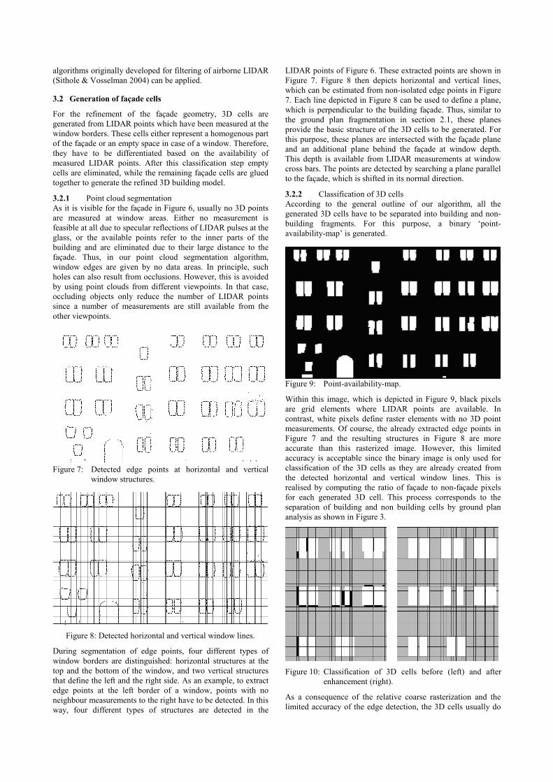
3.2.2 Classification of 3D cells According to the general outline of our algorithm, all the generated 3D cells have to be separated into building and non-building fragments. For this purpose, a binary ‘point-availability-map’ is generated.

Figure 9: Point-availability-map.

Within this image, which is depicted in Figure 9, black pixels are grid elements where LIDAR points are available. In contrast, white pixels define raster elements with no 3D point measurements. Of course, the already extracted edge points in Figure 7 and the resulting structures in Figure 8 are more accurate than this rasterized image. However, this limited accuracy is acceptable since the binary image is only used for classification of the 3D cells as they are already created from the detected horizontal and vertical window lines. This is realised by computing the ratio of façade to non-façade pixels for each generated 3D cell. This process corresponds to the separation of building and non building cells by ground plan analysis as shown in Figure 3.

Figure 10: Classification of 3D cells before (left) and after enhancement (right).

As a consequence of the relative coarse rasterization and the limited accuracy of the edge detection, the 3D cells usually do

not comprise of facade pixels or window pixels, exclusively. Within the classification, 3D cells including more than 70% façade pixels are defined as façade solids, whereas 3D cells with less than 10% façade pixels are assumed to be window cells. These segments are depicted in Figure 10 as grey and white cells, respectively.

While most of the 3D cells can be classified reliably, the result is uncertain especially at window borders or in areas with little point coverage. Such cells with a relative coverage between 10% and 70% are represented by the black segments in the left image of Figure 10. For the final classification of these cells depicted in the right image of Figure 10, neighbourhood relationships as well as constraints concerning the simplicity of the resulting window objects are used. As an example, elements between two window cells are assumed to belong to the façade, so two small windows are reconstructed instead of one large window. This is justified by the fact that façade points have actually been measured in this area. Additionally, the alignment as well as the size of proximate windows is ensured. For this purpose the classification of uncertain cells is defined depending on their neighbours in horizontal and vertical direction. Within this process it is also guaranteed that the merge of window cells will result in convex window objects.

a)

b)

c)

Figure 11: Integration of additional façade cell.

As it is depicted in Figure 11, additional façade cells can be integrated easily if necessary. Figure 11a shows the LIDAR measurement for two closely neighboured windows. Since in this situation only one vertical line was detected, a single window is reconstructed (Figure 11b). To overcome this problem, a window objects is separated into two smaller cells by an additional façade cell. This configuration is kept, if it can be verified as a valid assumption if façade points were actually measured at this position (Figure 11c).

Figure 12: Refined facade of the reconstructed building.

The final result of the building façade reconstruction from terrestrial LIDAR is depicted in Figure 12. For this example window areas were cut out from the coarse model depicted in Figure 5. While the windows are represented by polyhedral cells, also curved primitives can be integrated in the reconstruction process. This is demonstrated exemplarily by the round-headed door of the building.

4. CONCLUSION

Within the paper, an approach for 3D building reconstruction based on cell decomposition was presented. As input data, 2D ground plans and 3D point clouds from airborne and terrestrial LIDAR were used. During the generation of intersecting planes by the combination of ground plan segments, buffer operations are used. By these means the aspired level of generation is defined. Thus, the extruded ground plan can be simplified according to the point density available from airborne LIDAR, which is used for roof reconstruction. Additionally, symmetry relations like coplanarity can be detected during the generation of the planes also for larger distances between different building parts since the extension of these planes is only limited by the subsequent intersection step. The cell decomposition also showed to be very flexible if additional detail has to be integrated. While in our approach windows are represented by indentations, a reconstruction based on cell decomposition can also be used to efficiently subtract such rooms from an existing 3D model if measurements in the interior of the building are available.

Still there is enough room for further algorithmic improvement. However, in our opinion the concept of generating 3D cells by the mutual intersection of planes already proved to be very promising and has a great potential for processes aiming at the reconstruction of building models at different scales.

5. REFERENCES

Brenner, C. [2004]. Modelling 3D Objects Using Weak CSG Primitives. IAPRS Vol. 35.

Böhm, J. & Haala, N. [2005]. Efficient Integration of Aerial and Terrestrial Laser Data for Virtual City Modeling Using LASERMAPS. IAPRS Vol. 36 Part 3/W19 ISPRS Workshop Laser scanning 2005 , pp.192-197.

Gorte, B. [2002]. Segmentation of TIN-Structured Surface Models. Proceedings Joint International Symposium on Geospatial Theory, Processing and Applications, on CDROM, 5p.

Hoffmann, C.M. [1989]. Geometric & Solid Modelling. Morgan Kaufmann Punblishers, Inc., San Mateo, CA.

Mäntylä, M. [1988]. An Introduction to Solid Modeling. Computer Science Press, Maryland, U.S.A.

Mayer, H. & S. Reznik [2005]. Building Façade Interpretation from Image Sequences. IAPRS Vol. 36-3/W24.

Rottensteiner, F. [2001] Semi-automatic extraction of buildings based on hybrid adjustment using 3D surface models and management of building data in a TIS. PhD. thesis TU Wien .

Sithole, G. & Vosselman, G. [2004]. Experimental comparison of filter algorithms for bare-earth extraction from airborne laser point clouds. ISPRS Journal of Photogrammetry and Remote Sensing 59(1-2), pp.85-101.