cell design and resource allocation for small cell networks

HAL Id: tel-00745594https://tel.archives-ouvertes.fr/tel-00745594v2

Submitted on 7 Mar 2014

HAL is a multi-disciplinary open accessarchive for the deposit and dissemination of sci-entific research documents, whether they are pub-lished or not. The documents may come fromteaching and research institutions in France orabroad, or from public or private research centers.

L’archive ouverte pluridisciplinaire HAL, estdestinée au dépôt et à la diffusion de documentsscientifiques de niveau recherche, publiés ou non,émanant des établissements d’enseignement et derecherche français ou étrangers, des laboratoirespublics ou privés.

Cell design and resource allocation for small cellnetworks

Sreenath Ramanath

To cite this version:Sreenath Ramanath. Cell design and resource allocation for small cell networks. Other [cs.OH].Université d’Avignon, 2011. English. NNT : 2011AVIG0194. tel-00745594v2

https://tel.archives-ouvertes.fr/tel-00745594v2

https://hal.archives-ouvertes.fr

THÈSE

présentée pour obtenir le grade de Docteur en Sciences de l’Université d’Avignon

SPÉCIALITÉ : Informatique

École Doctorale ED 536 «Sciences and Agrosciences»Laboratoire d’Informatique d’Avignon (UPRES No 4128)

Cell Design and Resource Allocation for Small CellNetworks

par

Sreenath Ramanath

Soutenue publiquement le 6 Octobre 2011 devant un jury composé de :

M. CHAHED Tijani Professeur, Telecom SudParis, France RapporteurM. BONALD Thomas Maître de conférences, Telecom ParisTech, France RapporteurM. ALTMAN Eitan Directeur de recherche, INRIA, France DirecteurM. DEBBAH Mérouane Professeur, Supelec, France Co-directeurM. GESBERT David Professeur, Eurecom, France ExaminateurM. KUMAR Vinod Directeur, Global Research Partnerships,

Alcatel Lucent, France Examinateur

This dissertation is carried out in the framework of the INRIA and Alcatel-Lucent BellLabs Joint Research Lab on Self Organized Networks.

To my parents, family, friends and teachers.

Part I

Prologue

5

Preface

It was a warm February evening (2008) in Bangalore that I met Dr. Eitan Altman thefirst time. He had just offered my wife, Kavitha, a post doc position at INRIA andwanted to know what were my plans. I was intending to take a sabbatical from my jobto support my wife’s research interests, when, he presented an irresistible offer: to behis student!. A dormant ambition, a desire to learn and the challenges of an untroddenpath beckoned me to a world of research. It is with great pleasure that i thank Eitan forgiving me this opportunity. His ideas, encouragement and support have gone a longway in understanding new topics and trends in wireless and networking research.

I would like to thank Dr. Philippe Nain for accepting me into the Maestro Group atINRIA, Sophia Antipolis and encouraging me to actively participate in group meetings,conferences and workshops.

I would like to acknowledge Laurant Thomas for accepting me to be a part of theINRIA-Bell Labs initiative on Self Organizing Networks and proposing a very interest-ing and happening research topic. I appreciate Dr. Vinod Kumar’s encouragement andinitiative to make me feel comfortable and settle down with research as well as life inFrance.

A fortnight into my arrival in France, i found a surprise mail. This opened up alot of new opportunities and dimensions in my research. Thank you Prof. MerouaneDebbah for being my thesis co-advisor and for your support and encouragement.

Over the course of my thesis, i was introduced to Laurant Roullet. I would like toacknowledge his interest and patience in understanding and encouraging me in myresearch.

Innovation is key in any research and i do hope to find some of the ideas presentedin this thesis to find use in practice. I would like to acknowledge Dr. Veronique Capdev-ille in showing interest in my research and encouraging me to participate in realizingthese in practice.

I would like to thank the administrative staff at INRIA, especially, Ephie Dericheand Laurie Vermeersch for being patient with our many queries and helping us to planvisits to conferences and workshops. I would like to acknowledge the administrativestaff at LIA, specifically, Simone Mouzac and Jocelyne Gourret for taking care of ourday to day requirements and activities.

7

I want to express my sincere gratitude to Prof. Tijani Chahed and Prof. ThomasBonald, who accepted to review the manuscript and Prof. David Gesbert and Dr. VinodKumar, who accepted to be my thesis examiners. Thankyou for your patient reading,valuable comments to improvise the thesis and kind words of encouragement.

A review comment sparked a thought process which resulted in a flash survey tofind the top five innovations and advancements in the field of wireless communica-tions in recent years. I would like to express my sincere thanks to many Professors,colleagues, colloborators and acquaintances who took part and shared their views.

I would like to thank my colleagues in INRIA, LIA and Supelec for many interestingdiscussions and words of encouragement. Special thanks go to Kostia, Tania, Rachid,Yezekael, Sabir, Tembine, Julio, Sulan, Yuedong, Amar, Manjesh, Baslam, Habib, Wis-sam, Romain, Alonso, Veronica, Leonardo, Antonia, Jakob, Salam and Subhash for theirtechnical as well as friendly interactions.

A special mention of Merci Beaucoup goes to Richard Combes for his help in writingthe thesis abstract in French (Résumé).

A very special thanks to my daughter, Prajna, who learnt and taught me French. Herschool, friends and activities made my everyday life more colorful, joyous and fun, notto mention the feeling of revisiting my childhood.

Coming back to Kavitha, she has been an inspiration which i couldn’t catch up!.Her willingness and dedication to understand and learn is exemplary. She has beena constant source of encouragement and help in understanding and solving many atricky twists and turns that came in the course of my research. I owe her a lot.

I wish to thank my parents, sisters and their families, my in-laws, for their uncondi-tioned love, encouragement and support.

And thanks to all my friends and relatives for their love and encouragement duringthe tenure of my studies.

Sep 2011, Avignon, France Sreenath Ramanath

8

Résumé

Récemment, il y a eu une hausse massive du trafic dans les réseaux mobiles à causede nouveaux services et applications. Les architectures actuelles des réseaux cellulairesne sont plus capables de gérer de façon satisfaisante ce trafic. Les Réseaux de PetitesCellules (RPC), basées sur un déploiement dense de stations de bases portables, auto-organisantes et efficaces en termes d’énergie apparait comme une solution prometteuseà ce problème. Les RPC augmentent la capacité du réseau, réduisent sa consommationénergétique et améliorent sa couverture. Par contre, elles posent des défis importantsen termes de design optimal.

Dans cette thèse, des aspects liés au design cellulaire et à l’allocation de ressourcesdans les RPC sont traités. La thèse se compose de deux parties.

Dans la première partie, le design cellulaire est étudié: une population statiqued’utilisateurs est considérée, et la taille optimale de cellule maximisant le débit spa-tial est donnée en fonction du modèle de récepteur, des conditions radio et des par-titions indoor/outdoor. En considérant des utilisateurs mobiles, la taille de celluleoptimale est étudiée afin de minimiser le temps de service, et minimiser le blocageet la déconnexion en cours de communication, en fonction de la vitesse des utilisa-teurs et du type de trafic. Le problème de placement des stations de base optimal esttraité en fonction de différents critères de qualité (maximisation de débit total, équitéproportionnelle, minimisation de délai, équité max-min) pour différentes distributionsd’utilisateurs et partitions de cellules. Le problème de scaling de capacité dans un RPClimité par l’interférence avec pré-codage est étudié, et la quantité optimale d’antennespar utilisateurs en fonction de l’interférence inter-cellules est dérivée. Dans le cadred’un réseau “green”, pour une charge du réseau donnée, on étudie les politiques op-timales en boucle ouverte, afin de maximiser soit une fonction coût du système (con-trôle centralisé) soit des fonctions de coût de chacune des stations de base (contrôledistribué).

Dans la seconde partie, nous étudions l’allocation de ressources, nous introduisonsles concepts de d’équité T-échelle et équité multi-échelle. Ces concepts permettentde distribuer les ressources équitablement pour les différentes classes de trafic. Cesconcepts sont illustrés par des applications au partage de spectre et à l’allocation deressources dans les femto-cellules indoor/outdoor. L’allocation de puissance pour sat-isfaire les demandes de trafic des utilisateurs avec un grand nombre d’interféreurs estune tâche difficile. Ce problème est abordé, et nous proposons un algorithme universel

9

qui converge vers une configuration de puissance optimale qui satisfait les demandesdes utilisateurs dans toutes les stations de base. Les performances de l’algorithme sontillustrées pour différentes configurations du système et différents niveaux de coopéra-tion entre les stations de base.

10

Abstract

An ever increasing demand for mobile broadband applications and services is lead-ing to a massive network densification. The current cellular system architectures areboth economically and ecologically limited to handle this. The concept of small-cellnetworks (SCNs) based on the idea of dense deployment of self-organizing, low-cost,low-power base station (BSs) is a promising alternative.

Although SCNs have the potential to significantly increase the capacity and cov-erage of cellular networks while reducing their energy consumption, they pose manynew challenges to the optimal system design.

Due to small cell sizes, the mobile users cross over many cells during the course oftheir service resulting in Frequent handovers. Also, due to proximity of base stations(BS), users (especially those at cell edges) experience a higher degree of interferencefrom neighboring base stations. If one has to derive advantages from small networks,these alleviated effects have to be taken care either by compromising on some aspectsof optimality (like dedicating extra resources) or by innovating smarter algorithms orby a combination of the two.

The concept of umbrella cells is introduced to take care of frequent handovers. Hereextra resources are dedicated to ensure that the calls are not dropped within an um-brella cell. To manage interference, one might have to ensure that the neighboringcells always operate in independent channels or design algorithms which work wellin interference dominant scenarios or use the backhaul to incorporate base station co-operation techniques. Further, small cell BS are most often battery operated, whichcalls for efficient power utilization and energy conservation techniques. Also, whendeployed in urban areas, some of the small cells can have larger concentration of usersthroughout the cell, for example, hot-spots, which calls in for design of small cell net-works with dense users. Also, with portable base stations, one has the choice to installthem on street infrastructure or within residential complexes. In such cases, cell designand resource allocation has to consider aspects like user density, distribution (indoor-outdoor), mobility, attenuation, etc.

We present the thesis in two parts. In the first part we study the cell design aspectswhile the second part deals with the resource allocation. While the focus is on smallcells, some of the results derived and the tools and techniques used are also applicableto conventional cellular systems.

11

In the first part, we study various aspects of cell design like cell dimensioning, basestation placement, optimal fraction of users per transmit antenna, base station(s) acti-vation policies etc.

For cell dimensioning, we consider two scenarios based on the mobility patternof the users. For systems supporting only static users (Chapter 2), under fluid limits(i.e., when the number of users is large), we compute the cell size that maximizes thespatial throughput density. For systems that support mobile users (Chapter 3), weuse the concept of umbrella cells. We model the small cell network using queueingtheoretic models and obtain cell size that optimizes various performance measures likeexpected waiting times, service times, call block and drop probabilities, etc. We nextforego this umbrella assumption and obtain the cell size that optimizes call block anddrop probabilities. We make some interesting observations like that the optimal cellsize is independent of the traffic type and that for a given power there is a limit velocitybeyond which useful communication ceases.

Once the cell dimensioning is done, further design rules tend to assume that the BSis centrally located. But, does the placement of BS matter? Does it change dependingon some criteria? We analyze this in the context of locating base stations (Chapter4) according to some fairness criterion. We show that the location of the base stationconverges to the center of the cell as the fairness parameter tends to infinity; i.e, themax-min fair BS placement is the center of the cell. Further, this is true independent ofthe underlying user density or characteristics of the cell (eg. indoor-outdoor partitions,hot-spots, etc.).

While, it is well known that dividing a large cell into number of small cells enhancesthe system capacity, the spatial dimension can be exploited to enhance the capacity fur-ther. In this aspect, we consider a MIMO broadcast channel (Chapter 5) and investigatethe effect of multi-cell interference in precoded small cell networks. We show that theirexists an optimal ratio of number of antennas at the BS to the number of users for agiven interference level. The problem is solved in the asymptotic limit using randommatrix theory and we show via numerical simulations that the asymptotic expressionsare reliable even in the finite case.

Cell design considering dense deployment of BS as in small cell networks need tobe energy efficient. We come up with optimal open loop BS activation policies (Chapter6), which depends on the system load. We use tools from multimodularity to derive thestructure of the optimal policies.

In the second part of the thesis, we address resource allocation. Resources are to beallocated so as to fair share the average utilities that corresponds to the assignments.But the exact definition of average share depends on the application! Different applica-tions require averaging over different time periods or time scales (eg., real time voice,file downloads, gaming, multimedia streaming). Hence fairness need to be definedover mixed timescales. In this context, we introduce T-scale and multiscale fairness(Chapter 7). This new concept allows one to distribute the network resources fairlyamong different classes of traffic. We illustrate this concept via some example applica-tions in spectrum allocation and in indoor-outdoor femtocells.

12

Futher, given that we have users with varying QoS demands, how do we allocatepower to satisfy their demands? What if we have different system architectures, sup-porting various standards and interfering with each other?. Is there a simple and effec-tive self-organizing power allocation mechanism, which can work for any or a combi-nation of these systems? We address this problem of power allocation to satisfy userdemand rates (Chapter 8) in a multicell network. We propose a simple and universalpower allocation algorithm which guarantees convergence to user demands, wheneverthe demands lie within the system specific rate region. This algorithm can work from acompletely centralized to a fully distributed setting. Further, with macrocells and smallcells co-existing, we propose an extension of the algorithm to multi-tier networks.

We have used a variety of tools to model and analyze the problems that arise indimensioning and resource allocation. Specifically, queueing theory, random matrixtheory, stochastic approximation, etc, have been used to understand, characterize andderive asymptotic results and practically implementable algorithms for self organizingnetworks.

Our hope is that this thesis will form a initial framework to explore and exploit themany dimensions that arise in designing optimal small cell systems, which will satisfythe next generation mobile broadband user.

13

Contents

I Prologue 5

Preface 7

Résumé 9

Abstract 11

1 Introduction 251.1 General introduction . . . . . . . . . . . . . . . . . . . . . . . . . . . . . . 251.2 Recent innovations and advances in wireless communication . . . . . . . 261.3 Small cell networks . . . . . . . . . . . . . . . . . . . . . . . . . . . . . . . 301.4 Thesis Overview . . . . . . . . . . . . . . . . . . . . . . . . . . . . . . . . 341.5 Tools used in the thesis . . . . . . . . . . . . . . . . . . . . . . . . . . . . . 351.6 Organization and Contributions . . . . . . . . . . . . . . . . . . . . . . . 37

II Cell Design 41

2 Cell Dimensioning with Static Users, a fluid perspective 432.1 Introduction . . . . . . . . . . . . . . . . . . . . . . . . . . . . . . . . . . . 43

2.1.1 Related work . . . . . . . . . . . . . . . . . . . . . . . . . . . . . . 442.2 Received Power computation . . . . . . . . . . . . . . . . . . . . . . . . . 45

2.2.1 Single frequency (SF) . . . . . . . . . . . . . . . . . . . . . . . . . . 452.2.2 Frequency reuse (FR) . . . . . . . . . . . . . . . . . . . . . . . . . . 46

2.3 Throughput . . . . . . . . . . . . . . . . . . . . . . . . . . . . . . . . . . . 472.3.1 Matched filter (MF) . . . . . . . . . . . . . . . . . . . . . . . . . . . 472.3.3 Multi-user detection (MD) . . . . . . . . . . . . . . . . . . . . . . . 482.3.5 Comments on the fluid approach . . . . . . . . . . . . . . . . . . . 50

2.4 Impact of cell size on throughput . . . . . . . . . . . . . . . . . . . . . . . 512.4.1 Numerical results . . . . . . . . . . . . . . . . . . . . . . . . . . . . 512.4.2 Optimizing the cell size . . . . . . . . . . . . . . . . . . . . . . . . 52

2.5 Indoor analysis . . . . . . . . . . . . . . . . . . . . . . . . . . . . . . . . . 532.5.1 BS located inside the building . . . . . . . . . . . . . . . . . . . . . 532.5.2 BS located outside the building . . . . . . . . . . . . . . . . . . . . 54

2.6 Dimension 2 . . . . . . . . . . . . . . . . . . . . . . . . . . . . . . . . . . . 54

15

2.6.1 A simple approximation to the hexagonal grid . . . . . . . . . . . 552.6.2 A more precise approximation for the 2-D hexagonal grid . . . . 572.6.3 Throughput density with reuse . . . . . . . . . . . . . . . . . . . . 572.6.4 Indoor analysis . . . . . . . . . . . . . . . . . . . . . . . . . . . . . 58

2.7 Coverage and capacity . . . . . . . . . . . . . . . . . . . . . . . . . . . . . 592.7.1 Coverage and capacity in a single cell . . . . . . . . . . . . . . . . 592.7.2 Coverage and capacity on a line segment (1D) . . . . . . . . . . . 612.7.3 Coverage and capacity in two dimension . . . . . . . . . . . . . . 62

2.8 Conclusions and future perspectives . . . . . . . . . . . . . . . . . . . . . 622.9 Publications . . . . . . . . . . . . . . . . . . . . . . . . . . . . . . . . . . . 63

3 Spatial Queueing Analysis for Design and Dimensioning of Small Cell Net-works with Mobile Users 653.1 Introduction . . . . . . . . . . . . . . . . . . . . . . . . . . . . . . . . . . . 653.2 System Model . . . . . . . . . . . . . . . . . . . . . . . . . . . . . . . . . . 683.3 System Analysis . . . . . . . . . . . . . . . . . . . . . . . . . . . . . . . . . 69

3.3.1 Time required for communicating S bytes (Bc) . . . . . . . . . . . 703.3.3 Maximum velocity handled by the system . . . . . . . . . . . . . 723.3.4 Service time : The time of the Macrocell spent for user’s service . 733.3.5 Macro Handovers . . . . . . . . . . . . . . . . . . . . . . . . . . . . 733.3.6 Moments of Service time . . . . . . . . . . . . . . . . . . . . . . . 743.3.7 Cell size optimizing the moments of the service time . . . . . . . 743.3.8 ES Calls : Average Waiting time . . . . . . . . . . . . . . . . . . . 753.3.9 NES Calls : Block and Drop Probabilities . . . . . . . . . . . . . . 77

3.4 Mobility on a street grid . . . . . . . . . . . . . . . . . . . . . . . . . . . . 783.5 Mobility Examples . . . . . . . . . . . . . . . . . . . . . . . . . . . . . . . 793.6 Call drops at Small cell boundaries (NES calls) . . . . . . . . . . . . . . . 80

3.6.2 Service Time : Time of the Small cell spent for user’s service . . . 813.6.3 Small cell Handovers . . . . . . . . . . . . . . . . . . . . . . . . . . 823.6.5 Stability Factor . . . . . . . . . . . . . . . . . . . . . . . . . . . . . 833.6.6 New Call Block Probability . . . . . . . . . . . . . . . . . . . . . . 833.6.7 Drop Probability . . . . . . . . . . . . . . . . . . . . . . . . . . . . 84

3.7 Conclusions and Future work . . . . . . . . . . . . . . . . . . . . . . . . . 853.8 Appendix M: Calculations related to Macro queue . . . . . . . . . . . . . 86

3.8.1 M.1 Proof of Theorem 3.3.3.1 . . . . . . . . . . . . . . . . . . . . . 863.8.2 M.2 Moments of service time and its derivatives . . . . . . . . . . 863.8.3 M.3 ν has an unique maximizer: . . . . . . . . . . . . . . . . . . . 873.8.4 M.4 Derivatives db(k)/dL vanish only at L∗

ν(v) when V ≡ v . . . . 873.9 Appendix P: Calculations for Small cell queue . . . . . . . . . . . . . . . 88

3.9.1 P.1 Small cell Handover Speed Distribution . . . . . . . . . . . . . 883.9.2 P.2 Small cell Stability Factor . . . . . . . . . . . . . . . . . . . . . 893.9.3 P.3 Drop probability . . . . . . . . . . . . . . . . . . . . . . . . . . 89

3.10 Publications . . . . . . . . . . . . . . . . . . . . . . . . . . . . . . . . . . . 90

4 Fair Assignment of Base Station Locations 914.1 Introduction . . . . . . . . . . . . . . . . . . . . . . . . . . . . . . . . . . . 91

16

4.2 Our model and assumptions . . . . . . . . . . . . . . . . . . . . . . . . . . 924.3 Large population limits and problem statement . . . . . . . . . . . . . . . 93

4.3.1 Power computation : . . . . . . . . . . . . . . . . . . . . . . . . . . 934.3.2 Throughput computation: . . . . . . . . . . . . . . . . . . . . . . . 944.3.3 α-fair placement criterion : . . . . . . . . . . . . . . . . . . . . . . . 954.3.4 Problem statement . . . . . . . . . . . . . . . . . . . . . . . . . . . 95

4.4 Analysis : Single BS Placement . . . . . . . . . . . . . . . . . . . . . . . . 964.4.1 Ptot(z) is independent of BS location z : . . . . . . . . . . . . . . . 964.4.5 Ptot(z) is dependent on BS location z : . . . . . . . . . . . . . . . . 98

4.5 Optimal and fair placement of a single BS . . . . . . . . . . . . . . . . . . 994.5.1 Outdoor cell . . . . . . . . . . . . . . . . . . . . . . . . . . . . . . . 994.5.2 Indoor-outdoor cell (Split-cell) . . . . . . . . . . . . . . . . . . . . 102

4.6 Optimal and fair placement of two BS in an outdoor cell . . . . . . . . . 1064.7 Conclusions and future perspectives . . . . . . . . . . . . . . . . . . . . . 1104.8 Appendix A : Large population limits - power, throughput and α-fair

placement of two base stations: . . . . . . . . . . . . . . . . . . . . . . . . 1104.9 Publications . . . . . . . . . . . . . . . . . . . . . . . . . . . . . . . . . . . 112

5 Asymptotic Analysis of Precoded Small Cell Networks 1135.1 Introduction . . . . . . . . . . . . . . . . . . . . . . . . . . . . . . . . . . . 1135.2 Random Matrix Theory Tools . . . . . . . . . . . . . . . . . . . . . . . . . 1155.3 System model and assumptions . . . . . . . . . . . . . . . . . . . . . . . . 1165.4 Channel inversion precoding . . . . . . . . . . . . . . . . . . . . . . . . . 117

5.4.1 Single cell . . . . . . . . . . . . . . . . . . . . . . . . . . . . . . . . 1175.4.2 Asymptotic analysis for a single-cell . . . . . . . . . . . . . . . . . 1185.4.3 Optimizer β∗ for the single cell . . . . . . . . . . . . . . . . . . . . 1195.4.4 Multi-cell . . . . . . . . . . . . . . . . . . . . . . . . . . . . . . . . 1205.4.5 Asymptotic analysis for the multi-cell . . . . . . . . . . . . . . . . 1215.4.7 Optimizer β∗ for the multi-cell . . . . . . . . . . . . . . . . . . . . 1225.4.8 Some observations: . . . . . . . . . . . . . . . . . . . . . . . . . . . 1235.4.9 Single cell and multi-cell with unequal power . . . . . . . . . . . 124

5.5 Simulation results . . . . . . . . . . . . . . . . . . . . . . . . . . . . . . . . 1265.6 Conclusions . . . . . . . . . . . . . . . . . . . . . . . . . . . . . . . . . . . 1275.7 Publications . . . . . . . . . . . . . . . . . . . . . . . . . . . . . . . . . . . 129

6 Open Loop Control of BS Deactivation 1316.1 Introduction . . . . . . . . . . . . . . . . . . . . . . . . . . . . . . . . . . . 1316.2 Multimodularity . . . . . . . . . . . . . . . . . . . . . . . . . . . . . . . . 1336.3 Centralized optimal control . . . . . . . . . . . . . . . . . . . . . . . . . . 1346.4 Decentralized optimal control . . . . . . . . . . . . . . . . . . . . . . . . . 1366.5 Future Directions . . . . . . . . . . . . . . . . . . . . . . . . . . . . . . . . 1376.6 Conclusions . . . . . . . . . . . . . . . . . . . . . . . . . . . . . . . . . . . 1386.7 Publications . . . . . . . . . . . . . . . . . . . . . . . . . . . . . . . . . . . 141

17

III Resource Allocation 143

7 Multiscale Fairness and its Application in Wireless Networks 1457.1 Introduction . . . . . . . . . . . . . . . . . . . . . . . . . . . . . . . . . . . 1457.2 Resource Sharing model and different fairness definitions . . . . . . . . . 147

7.2.1 Fairness over time: Instantaneous Versus Long term α-fairness . 1487.2.2 Fairness over time: T-scale α-fairness . . . . . . . . . . . . . . . . 1507.2.3 Fairness over different time scales: Multiscale fairness . . . . . . 152

7.3 Instantaneous α-fairness for linear resources . . . . . . . . . . . . . . . . 1537.4 Application to spectrum allocation in random fading channels . . . . . . 1557.5 Application to indoor-outdoor scenario . . . . . . . . . . . . . . . . . . . 160

7.5.1 Instantaneous Fairness . . . . . . . . . . . . . . . . . . . . . . . . . 1617.5.2 Long term Fairness . . . . . . . . . . . . . . . . . . . . . . . . . . . 162

7.6 Conclusion and Future Research . . . . . . . . . . . . . . . . . . . . . . . 1647.7 Publications . . . . . . . . . . . . . . . . . . . . . . . . . . . . . . . . . . . 164

8 Satisfying Demands in Multicell Networks: A Universal Power AllocationAlgorithm 1658.1 Introduction . . . . . . . . . . . . . . . . . . . . . . . . . . . . . . . . . . . 1658.2 System model . . . . . . . . . . . . . . . . . . . . . . . . . . . . . . . . . . 1678.3 System specific problem formulation . . . . . . . . . . . . . . . . . . . . . 169

8.3.1 Game theoretic formulation . . . . . . . . . . . . . . . . . . . . . . 1718.4 Universal Algorithm : UPAMCN . . . . . . . . . . . . . . . . . . . . . . . 173

8.4.1 UPAMCN algorithm . . . . . . . . . . . . . . . . . . . . . . . . . . 1738.4.2 Analysis . . . . . . . . . . . . . . . . . . . . . . . . . . . . . . . . . 1748.4.3 Analysis of the specific systems . . . . . . . . . . . . . . . . . . . 1748.4.5 Extensions to UPAMCN . . . . . . . . . . . . . . . . . . . . . . . . 175

8.5 Simulation . . . . . . . . . . . . . . . . . . . . . . . . . . . . . . . . . . . . 1758.6 Conclusions . . . . . . . . . . . . . . . . . . . . . . . . . . . . . . . . . . . 1788.7 Appendix A: Example Systems . . . . . . . . . . . . . . . . . . . . . . . . 1788.8 Appendix B: Proofs . . . . . . . . . . . . . . . . . . . . . . . . . . . . . . . 1808.9 Publications . . . . . . . . . . . . . . . . . . . . . . . . . . . . . . . . . . . 181

IV Epilogue 183

9 Conclusions 185

Appendix 189

Publications 195

References 197

18

List of Figures

1.1 Evolution of wireless applications and services (Qualcomm [112]) . . . . 301.2 Example of heterogeneous network deployment with macrocells com-

plemented by relays and pico/femto cells (Guillaume de la Roche, et.al., [50]) . . . . . . . . . . . . . . . . . . . . . . . . . . . . . . . . . . . . . . 31

1.3 Traffic demand (Claussen [44]) . . . . . . . . . . . . . . . . . . . . . . . . 321.4 Mobile data forecast (Cisco [154]) . . . . . . . . . . . . . . . . . . . . . . . 321.5 Example of Pico cell deployment serving static and moving users . . . . 331.6 Possible alternatives to support mobility in small cells (Alcatel Lucent -

Bell Labs [4]) . . . . . . . . . . . . . . . . . . . . . . . . . . . . . . . . . . . 34

2.1 Frequency allocation in 1D. . . . . . . . . . . . . . . . . . . . . . . . . . . 442.2 Total power received at the BS in C0 vs L (α = 2, 4; single frequency). . . 542.3 Total power density from C0 vs L (α = 2, 4; single frequency, matched

filter). . . . . . . . . . . . . . . . . . . . . . . . . . . . . . . . . . . . . . . . 542.4 Total throughput of cell C0 vs L (α = 2). . . . . . . . . . . . . . . . . . . . 552.5 Throughput density vs L (α = 2). . . . . . . . . . . . . . . . . . . . . . . . 562.6 Throughput density vs L (α = 4). . . . . . . . . . . . . . . . . . . . . . . . 562.7 Throughput density vs L (α = 2, wall attenuation 12dB, BS indoors). . . 562.8 Throughput density vs L (α = 2, wall attenuation 12dB, BS outdoors). . . 562.9 Optimal cell size L∗ vs path-loss factor α (reuse factor m = 1) . . . . . . . 562.10 width=7cm . . . . . . . . . . . . . . . . . . . . . . . . . . . . . . . . . . . . 562.11 Frequency allocation in 2D. . . . . . . . . . . . . . . . . . . . . . . . . . . 592.12 Throughput density vs L for different α and decoding schemes compar-

ing MethodA with MethodB. . . . . . . . . . . . . . . . . . . . . . . . . . . 602.13 Throughput density vs L for α = 4.1 and different reuse factors. . . . . . 602.14 Throughput density vs L for α = 4.1 and different reuse factors (BS in-

doors). . . . . . . . . . . . . . . . . . . . . . . . . . . . . . . . . . . . . . . 602.15 Throughput density vs L for α = 4.1 and different reuse factors (indoor

cell, BS outdoors). . . . . . . . . . . . . . . . . . . . . . . . . . . . . . . . . 602.16 Capacity vs cell coverage x for α = 2, 4. . . . . . . . . . . . . . . . . . . . 602.17 Throughput density vs L for 100 % and 75 % cell coverage (α = 2, 1D). . 612.18 Throughput density vs L for 100 % and 75 % cell coverage (α = 4.1,

multi-user detection, 2D). . . . . . . . . . . . . . . . . . . . . . . . . . . . 61

3.1 User moving with velocity V along a line . . . . . . . . . . . . . . . . . . 68

19

3.2 Approximation of Communication time, Bc . . . . . . . . . . . . . . . . . 723.3 2D network for rectangular-grid small cell networks . . . . . . . . . . . . 793.4 Moments of the service time and the expected waiting time versus L. . . 793.5 Optimal cell size versus mean velocity for different variances. . . . . . . 803.6 Optimal cell size versus variance of the velocity. . . . . . . . . . . . . . . 80

4.1 Open-cell: BS located at z, user density λ(x) = x . . . . . . . . . . . . . . 1004.2 Open cell: Global throughput (4.3) as a function of the BS location. User

density λ(x) = x and β = 2) . . . . . . . . . . . . . . . . . . . . . . . . . . 1014.3 Proportional fair objective function fα given by (4.4) with α ≈ 1, as func-

tion of BS location z. User density λ(x) = x, β = 2) . . . . . . . . . . . . 1014.4 Harmonic fair objective function fα given by (4.4) with α = 2, as function

of BS location z. User density λ(x) = x, β = 2) . . . . . . . . . . . . . . . 1014.5 α-fair BS location, z∗(α) as a function of α. . . . . . . . . . . . . . . . . . 1014.6 Split-cell: BS located at z, wall located at y . . . . . . . . . . . . . . . . . . 1034.7 Split-cell: Global throughput (Objective function fα(z) (4.6) with α = 0)

as a function of BS location z. . . . . . . . . . . . . . . . . . . . . . . . . . 1044.8 Split-cell: Objective function fα(z) (4.7) for proportional fairness (α =

0.99) as a function of BS location z. . . . . . . . . . . . . . . . . . . . . . . 1044.9 Split-cell: Objective function fα(z) (4.7) for harmonic fairness (α = 2) as

a function of BS location z. . . . . . . . . . . . . . . . . . . . . . . . . . . . 1044.10 Split-cell: α-fair BS location z∗(α) as a function of α. . . . . . . . . . . . . 1044.11 Split-cell: Global throughput (4.6) as a function of BS location z and wall

location y. . . . . . . . . . . . . . . . . . . . . . . . . . . . . . . . . . . . . 1054.12 Split-cell: Global throughput (4.6) as a function of BS location z and at-

tenuation η. . . . . . . . . . . . . . . . . . . . . . . . . . . . . . . . . . . . 1054.13 Open-cell: BS1 located at z1, BS2 located at z2, user density λ(x) ≡ 1/2D 1074.14 Outdoor cell, two BS: Global throughput (objective function fα(z1, z2)

with α = 0) as a function of BS1 location (z2 = −z1)). . . . . . . . . . . . 1084.15 Outdoor cell, two BS: Global throughput (objective function fα(z1, z2)

with α = 0) as a function of BS2 location(z1 = −z2)). . . . . . . . . . . . . 1084.16 Outdoor cell, two BS: 3-D contour plot of global throughput (objective

function fα(z1, z2) with α = 0) as a function of BS locations (z1, z2) . . . . 1084.17 Outdoor cell, two BS: α-fair BS location z∗2(α) as a function of α (Place-

ment of BS2 shown here). . . . . . . . . . . . . . . . . . . . . . . . . . . . 108

5.1 System model: multi-cell network. BS with M antennas, serving K users.Users at X experience nominal interference and users at Y experiencehigh interference . . . . . . . . . . . . . . . . . . . . . . . . . . . . . . . . 114

5.2 β∗ vs SNR for various interference factors (M = 16) . . . . . . . . . . . . 1235.3 K∗ vs SNR for various interference factors (M = 16) . . . . . . . . . . . . 1235.4 Sum rate at β∗ for various interference factors (M = 16) . . . . . . . . . . 1245.5 Sum rate at β = 2 for various interference factors (M = 16) . . . . . . . . 1245.6 Rate per antenna vs β at SNR of 20 dB for various interference factors γ 1285.7 Rate per antenna vs γ, when, β = 2, SNR ρ = 20 dB for various interfer-

ence factors γ . . . . . . . . . . . . . . . . . . . . . . . . . . . . . . . . . . 128

20

5.8 Sum rate per antenna as a function of M for β = 2 at SNR of 0 dB forvarious interference factors . . . . . . . . . . . . . . . . . . . . . . . . . . 128

5.9 Sum rate per antenna as a function of M for β = 2 at SNR of 20 dB forvarious interference factors . . . . . . . . . . . . . . . . . . . . . . . . . . 128

7.1 Performance index of [2,1] (dashed line) and [1,2] (solid line) assign-ments as a function of α (horizontal axis) . . . . . . . . . . . . . . . . . . 151

7.2 Performance index of [2,1] (dashed line) and [2,2] (solid line) assign-ments as a function of α (horizontal axis) . . . . . . . . . . . . . . . . . . 151

7.3 Throughput(θ) as a function of α for instantaneous, mid-term, long-termand (1,∞)-scale fairness criteria (Case 1). . . . . . . . . . . . . . . . . . . . 160



7.6 Coefficient of variation in expected throughput as a function of α for in-stantaneous, mid-term, long-term and (1,∞)-scale fairness criteria (Case3). . . . . . . . . . . . . . . . . . . . . . . . . . . . . . . . . . . . . . . . . . 161

7.7 Scheduler s∗ for the indoor and outdoor user with instantaneous fairnessas a function of α for α > 1. Wall attenuation 6 dB, path-loss β = 3,position of outdoor user x = −3. . . . . . . . . . . . . . . . . . . . . . . . 162

7.8 Throughput θ for the indoor and outdoor user with instantaneous fair-ness as a function of α for α > 1. Wall attenuation 6 dB, path-loss β = 3,position of outdoor user x = −3. . . . . . . . . . . . . . . . . . . . . . . . 162

7.9 l(α) for long-term fairness as a function of α (α > 1) and wall attenuationof 6 dB ,path-loss β = 2, position of outdoor user x = −2. . . . . . . . . . 163

8.1 2D Wyner model . . . . . . . . . . . . . . . . . . . . . . . . . . . . . . . . 1698.2 Rate convergence for Systems S1, S2 and S3 (H1 Network) . . . . . . . . 1768.3 Power convergence for Systems S1, S2 and S3 (H1 Network) . . . . . . . 1768.4 Demand satisfying NE. System S2. (L1, L2 & H1 networks) . . . . . . . . 1768.5 Rate convergence for System S4 and S5 (H2 Network) . . . . . . . . . . . 1778.6 Power convergence for Systems S4 and S5 (H2 Network) . . . . . . . . . 177

21

List of Tables

1.1 Evolution of wireless generations . . . . . . . . . . . . . . . . . . . . . . . 26

2.1 total received power as a function of α . . . . . . . . . . . . . . . . . . . . 462.2 Interference contribution for different reuse factors. . . . . . . . . . . . . 58

4.1 Outdoor cell: The α-fair BS locations and normalized throughput. Userdensity λ(x) = x, L = 10 and path-loss β = 2 . . . . . . . . . . . . . . . . 100

4.2 Outdoor cell: BS placement for globally-fair throughput for various path-loss β. User density λ(x) = x and L = 10 . . . . . . . . . . . . . . . . . . 102

4.3 Outdoor cell: BS placement for globally-fair throughput for various noise-variance σ2. User density λ(x) = x, path-loss β = 2 and L = 10 . . . . . 102

4.4 Split-cell: The α-fair BS location and normalized throughput. User den-sity λ(x) ≡ 1/2D, L = 10, y = 0.75L, path-loss β = 2 and wall attenua-tion η = 12dB . . . . . . . . . . . . . . . . . . . . . . . . . . . . . . . . . . 105

4.5 Split cell: BS placement for globally-fair throughput for various path-lossβ. User density λ(x) ≡ 1/2D and L = 10 . . . . . . . . . . . . . . . . . . 106

4.6 Split cell: BS placement for globally-fair throughput for various noise-variance σ2. User density λ(x) ≡ 1/2D, path-loss β = 2 and L = 10 . . . 106

4.7 The α-fair BS location(s) and normalized throughput for outdoor cellwith two BS, user density λ(x) = 1/2L, L = 10, path-loss β = 2 . . . . . 109

4.8 Outdoor cell with two BS: BS placement for globally-fair throughput forvarious path-loss β. User density λ(x) = 1/2L and L = 10 . . . . . . . . 109

7.1 Case 1,2 & 3: Shannon capacity (q)/probability(π) . . . . . . . . . . . . . 159

23

Chapter 1

Introduction

1.1 General introduction

Emergence of a variety of standards for Wireless Communication Networks in culmina-tion with advances in Radio Access Technologies offer increased reach, higher capacity,improved quality of service and many more things, while reducing energy consump-tion and deployment costs, paving the way for new applications and services in mobilebroadband access.

A pioneer of a computer networking systems is ALOHAnet [2], popularly knownas ALOHA, developed at the University of Hawaii, which became operational in 1971,providing the first demonstration of a wireless data network.

ALOHA used experimental UHF frequencies to begin with; as frequency assign-ments for commercial applications were not available in the 1970s. Further, ALOHAwas used in cable (Ethernet based) and satellite (Immarsat) applications. In the early1980s frequencies for mobile networks became available, and in 1985 frequencies suit-able for Wi-Fi were allocated in the US. These regulatory developments made it possibleto use ALOHA in both Wi-Fi and in mobile telephone networks. Since then ALOHAhas found applications across a multitude of wireline and wireless technologies.

While ALOHA has been a pioneer networking system, which spanned across wire-line and wireless networks, the wireless technology itself has evolved over the past fewyears from using analog FM transmission for voice telephony to OFDM / OFDMA formobile intenet and video streaming applications in the recent years. In table 1.1, wesummarize the evolution of wireless generations over the past few decades [158].

25

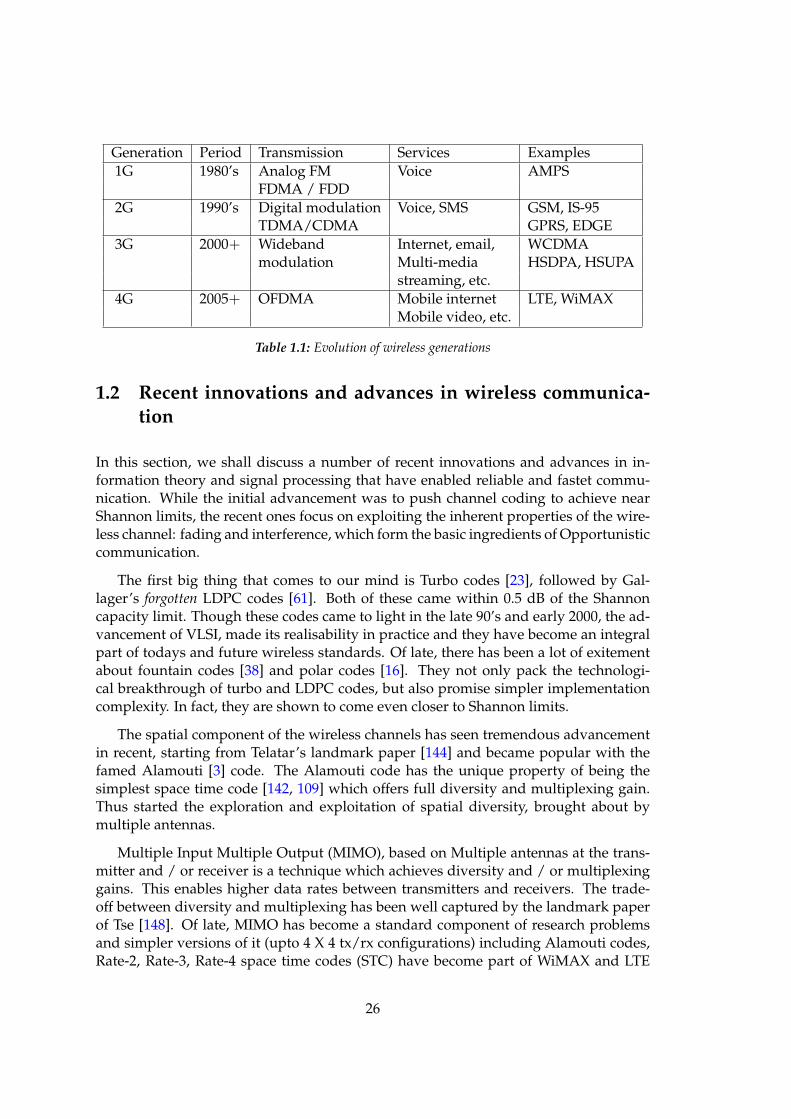
Generation Period Transmission Services Examples1G 1980’s Analog FM Voice AMPS

FDMA / FDD2G 1990’s Digital modulation Voice, SMS GSM, IS-95

TDMA/CDMA GPRS, EDGE3G 2000+ Wideband Internet, email, WCDMA

modulation Multi-media HSDPA, HSUPAstreaming, etc.

4G 2005+ OFDMA Mobile internet LTE, WiMAXMobile video, etc.

Table 1.1: Evolution of wireless generations

1.2 Recent innovations and advances in wireless communica-tion

In this section, we shall discuss a number of recent innovations and advances in in-formation theory and signal processing that have enabled reliable and fastet commu-nication. While the initial advancement was to push channel coding to achieve nearShannon limits, the recent ones focus on exploiting the inherent properties of the wire-less channel: fading and interference, which form the basic ingredients of Opportunisticcommunication.

The first big thing that comes to our mind is Turbo codes [23], followed by Gal-lager’s forgotten LDPC codes [61]. Both of these came within 0.5 dB of the Shannoncapacity limit. Though these codes came to light in the late 90’s and early 2000, the ad-vancement of VLSI, made its realisability in practice and they have become an integralpart of todays and future wireless standards. Of late, there has been a lot of exitementabout fountain codes [38] and polar codes [16]. They not only pack the technologi-cal breakthrough of turbo and LDPC codes, but also promise simpler implementationcomplexity. In fact, they are shown to come even closer to Shannon limits.

The spatial component of the wireless channels has seen tremendous advancementin recent, starting from Telatar’s landmark paper [144] and became popular with thefamed Alamouti [3] code. The Alamouti code has the unique property of being thesimplest space time code [142, 109] which offers full diversity and multiplexing gain.Thus started the exploration and exploitation of spatial diversity, brought about bymultiple antennas.

Multiple Input Multiple Output (MIMO), based on Multiple antennas at the trans-mitter and / or receiver is a technique which achieves diversity and / or multiplexinggains. This enables higher data rates between transmitters and receivers. The trade-off between diversity and multiplexing has been well captured by the landmark paperof Tse [148]. Of late, MIMO has become a standard component of research problemsand simpler versions of it (upto 4 X 4 tx/rx configurations) including Alamouti codes,Rate-2, Rate-3, Rate-4 space time codes (STC) have become part of WiMAX and LTE

26

standards. Multiple antenna transmissions also makes it possible to offer better QoS tocell edge users by cleverly beamforming or precoding the transmissions towards them.

Coming to multiplexing techniques, CDMA (Code Division Multiple Access) wasthe popular choice of 90’s, while OFDM (Orthogonal Frequency Disision Multiplexing[40]) has become the defacto in the 2000s. The advancement in signal processing in cul-mination with the gains of narrow band signalling has made OFDM a popular choicein todays modems. The biggest disadvantage comes from fluctuations in the signal lev-els when the frequency domain information is converted to time domain via FFT. Theextent of these fluctuations are measured by the metric peak to average power ratio(PAPR), which can be as high as 15-20 dB and large PAPR leads to problems with thedesign of power amplifiers (larger dynamic range). With the advancement in PAPR re-duction techniques, using both signal processing and RF techniques and with improvedpower amplifier technology, this issue seems to be well taken care off and OFDM is hereto stay.

OFDMA [169] is a multiple access technique based on OFDM. Here, the availablesub carriers spreading across the spectrum of interest is split amongst multiple users.With this it is possible to choose a cluster of sub-carriers and users in an optimal wayto combat fading and achieve diversity as well.

Ultra wide band (UWB) [163] was talked about a lot in recent years. This is a mod-ulation scheme which uses narrow (time domain) pulses spreading over multiple GHzof frequency spectrum. They were proposed for multiple applications including shortrange communications (Personal Area Networks: communication over few tens of me-ters). Though there was a huge surge of interest initially, in recent years, it is still wait-ing to take off owing to spectral and economic viability issues.

We come back to our initial discussion about the two fundamental properties ofwireless channel and discuss how in recent years, these are further exploited to improvespectral efficiency and resource utilization.

The fading nature of wireless channels is exploited to advantage via Opportunisticcommunication [72]. This involves the transmitters being aware of the channel towardsits users (via feedback) and favoring those users with better channel conditions. Sincefading is a time/frequency varying phenomenon, everyone stands to benefit over someaveraging duration. Further, fair schedulers [91] can be employed to guarentee certainQoS, even to disadvantaged users (cell edge or non LOS).

The other interesting idea of opportunistic communication is the principle of Cog-nitive radio [83]. This exploits unused spectrum and transmission opportunities ofprimary subscribers to schedule secondary users.

Relaying [80], yet another aspect of Opportunistic communication, manages inter-fernce and improve end to end QoS. Signals from transmitters to receivers are routedthrough relays which offer the best channel conditions. Also, due to the reduced trans-mission ranges, power budgets are reduced and hence interfernce. The disadvantage isthe extra resouces needed to setup and maintain relays.

27

Of late, co-operative as well as distributive strategies are gaining popularity. Co-operative strategies like multi cell co-opertion [67, 80] aim at managing interfernce ac-tively. At any given time the channel state of the entire system is known and a cen-tral controller can now decide the most optimal way the communciation happens be-tween individual transmitters and receivers. Recently, using these strategies, it has beenshown that the multicell capacity is same as the single cell capacity multiplied by thenumber of cells [67]. However, in practice, due to multiple limitations involving back-haul, latency, processing power, etc., sub-optimal schemes like clustering [67, 80], wherefew neighboring base stations (e.g, clustering) share the channel state or schemes thatuse a very minimal form of channel states like channel statistics have been proposedto make it possible for practical realization. Some of these are already underway forstandardization.

Decentralized and distributed processing is becoming popular to manage the com-plexity of central control. Here, each agent (base station), simultaneously updates itsparameters (runs an algorithm) to achieve a certain purpose. For example, each basestation could run a power allocation algorithm to meet its users demands with powerbudget contraints, while exchanging minimal information (channel statistics, rates allo-cated, etc.,) with its neighbours. Thus distributed processing becomes an essential partof a self organizing system, guaranteeing a certain minimum QoS to each user. Eachagent (base station / mobile) learns and adapts to the environment and thus managesto do the best. This is where the concepts of learning and adaptive algorithms comein. Reinforcement learning [165, 138], stochastic approximation [93], etc are becomingan integral part of new generation base stations. Game theory [11] and ODE (OrdinaryDifferntial Equations) tools are extensively used to formulate, analyze and understandthe behaviour of these algorithms.

Another point to mention is the recent surge in usage of tools like stochastic ge-ometry to analyze cellular networks [17]. The traditional methods of network analysisassumes linear or hexagonal networks. Stochastic geometry takes into account the ran-dom location (distribution) of transmit and receive nodes, which is a more realisitcassumption and many a times, it is possible to obtain explicit expressions for impor-tant system metrics. For example, one can compute explicit expressions for the totalinterference at a base station with simultaneous transmissions from randomly locatednodes, distributed according to a poisson process [17]. This can be plugged into theSignal to Interference plus Noise (SINR) equations to get a more realistic value as com-pared to a idealized value with regular placement of nodes. Thus the upper boundsand lower bounds of system metrics become more tighter. Though this is an emergingidea, it is still very difficult to analyze systems with spatial randomness and one oftenis comfortable using the popular Wyner-type cellular modelling [166] to get first cutunderstanding of new advancements like multi cell co-operation strategies [67].

Current view: With all these discussions, a point to ponder is that some of the inno-vations and advancements are a promise for the future, what about today? We need tofind a quicker solution to meet todays smart phones, gaming devices and tablets needs.This is where topology comes to aid technology. Dividing a large cell into number ofsmall cells [107, 49, 44, 82, 52] fits the old adage ’divide and conquer’. The reduced

28

cell sizes improve capacity and coverage. There are drawbacks related to infrastruc-tural costs, backbone, mobility induced frequent handovers, etc. Some of these, weshall address in due course. But, small cells appear promising to overcome coverageand capacity bottlenecks of todays applications. Also, it is a matter of time before thetechnical advancements we discussed become integral part of the small cell technology.

A recent survey: With so many new and exiting possibilites as discussed in previ-ous paragraphs, we wanted to know what were the most landmark innovations andadvancements in recent years as seen by experts in the research and engineering com-munity. We prepared a simple survey to identify the top few innovations and advance-ments in wirless communications and predict the next big thing in Information theory.We got some very interesting view points (See Appendix 9). Some said the survey itselfwas very thought provoking and needs careful thinking. Others felt that the guessinggame is difficult, citing examples of LDPC. Few others opined that it is all related tosimplicity of the idea, ease of implementation, standardization and economics of de-ployment. Citing from law of large numbers (of opinions), the top five without anyparticular order were Turbo/LDPC codes, OFDMA, MIMO, Opportunistic communi-cation and Multicell co-operative networks. The answer for the next big thing: Networkinformation theory.

Topology vs. Technology: Let us now illustrate via a few examples as to how reduc-ing the cell size turns out to be more beneficial when combined with recente technicaladvancements.

For example, opportunistic communication aims at scheduling and allocating userswhich have good channel conditions. Users close to the base station enjoy the benefitsof such schemes owing to better channel conditions (better signal strength, LOS compo-nents, etc.), while users at cell edge are disadvantaged. To circumvent this, a base sta-tion can employ a proportional-fair scheduler to improve the QoS of the cell edge user,but, this will be at the cost of decreasing the QoS for users with better channel condi-tions. Thus decreasing the cell size benefits opportunistic communication schemes andalso increases the fairness in the system.

Another example, OFDMA, aims at dividing the available sub-carriers amongst theusers to avail the benefits of frequency non-selective transmissions. But, again the lim-itations are apparent as one has to allocate more number of sub-carriers to cell edgeusers to maintain the QoS of the link. Shrinking the cell size translates to meeting thesame QoS with lesser number of sub-carriers. The left over sub-carriers can be used tosupport additional users for example.

Multiple antennas at the base station and users can dramatically improve the achiev-able capacity on a given link. Beam forming or precoding can effectively focus a beamto create better SINR conditions for cell edge users, while reducing interference towardsother users. But, this comes at the cost of using more resources at the transmitter. Forexample, a significant portion of the available power from the total power budget at thebase station is used towards the cell edge users. Bringing the cell edges closer, powerallocation towards the cell edge users dramatically decreases.

29

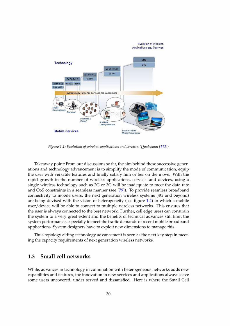
Figure 1.1: Evolution of wireless applications and services (Qualcomm [112])

.

Takeaway point: From our discussions so far, the aim behind these successive gener-ations and technology advancement is to simplify the mode of communication, equipthe user with versatile features and finally satisfy him or her on the move. With therapid growth in the number of wireless applications, services and devices, using asingle wireless technology such as 2G or 3G will be inadequate to meet the data rateand QoS constraints in a seamless manner (see [79]). To provide seamless broadbandconnectivity to mobile users, the next generation wireless systems (4G and beyond)are being devised with the vision of heterogeneity (see figure 1.2) in which a mobileuser/device will be able to connect to multiple wireless networks. This ensures thatthe user is always connected to the best network. Further, cell edge users can constrainthe system to a very great extent and the benefits of technical advances still limit thesystem performance, especially to meet the traffic demands of recent mobile broadbandapplications. System designers have to exploit new dimensions to manage this.

Thus topology aiding technology advancement is seen as the next key step in meet-ing the capacity requirements of next generation wireless networks.

1.3 Small cell networks

While, advances in technology in culmination with heterogeneous networks adds newcapabilities and features, the innovation in new services and applications always leavesome users uncovered, under served and dissatisfied. Here is where the Small Cell

30

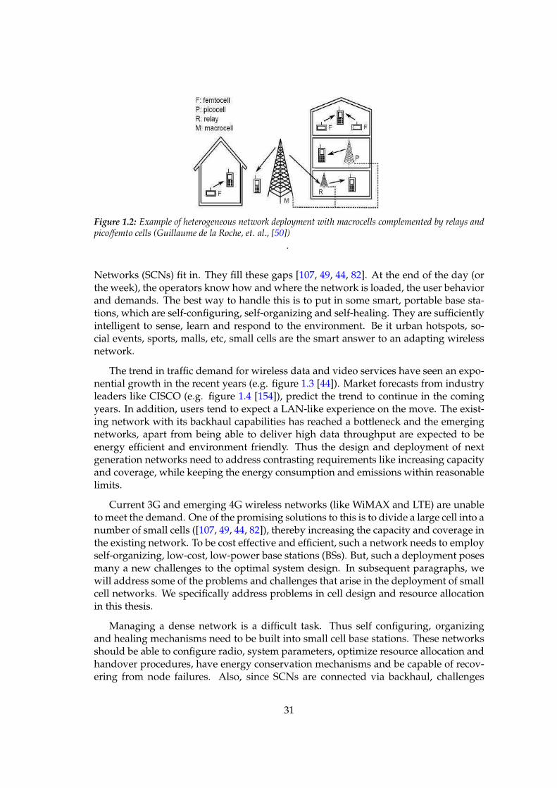
Figure 1.2: Example of heterogeneous network deployment with macrocells complemented by relays andpico/femto cells (Guillaume de la Roche, et. al., [50])

.

Networks (SCNs) fit in. They fill these gaps [107, 49, 44, 82]. At the end of the day (orthe week), the operators know how and where the network is loaded, the user behaviorand demands. The best way to handle this is to put in some smart, portable base sta-tions, which are self-configuring, self-organizing and self-healing. They are sufficientlyintelligent to sense, learn and respond to the environment. Be it urban hotspots, so-cial events, sports, malls, etc, small cells are the smart answer to an adapting wirelessnetwork.

The trend in traffic demand for wireless data and video services have seen an expo-nential growth in the recent years (e.g. figure 1.3 [44]). Market forecasts from industryleaders like CISCO (e.g. figure 1.4 [154]), predict the trend to continue in the comingyears. In addition, users tend to expect a LAN-like experience on the move. The exist-ing network with its backhaul capabilities has reached a bottleneck and the emergingnetworks, apart from being able to deliver high data throughput are expected to beenergy efficient and environment friendly. Thus the design and deployment of nextgeneration networks need to address contrasting requirements like increasing capacityand coverage, while keeping the energy consumption and emissions within reasonablelimits.

Current 3G and emerging 4G wireless networks (like WiMAX and LTE) are unableto meet the demand. One of the promising solutions to this is to divide a large cell into anumber of small cells ([107, 49, 44, 82]), thereby increasing the capacity and coverage inthe existing network. To be cost effective and efficient, such a network needs to employself-organizing, low-cost, low-power base stations (BSs). But, such a deployment posesmany a new challenges to the optimal system design. In subsequent paragraphs, wewill address some of the problems and challenges that arise in the deployment of smallcell networks. We specifically address problems in cell design and resource allocationin this thesis.

Managing a dense network is a difficult task. Thus self configuring, organizingand healing mechanisms need to be built into small cell base stations. These networksshould be able to configure radio, system parameters, optimize resource allocation andhandover procedures, have energy conservation mechanisms and be capable of recov-ering from node failures. Also, since SCNs are connected via backhaul, challenges

31

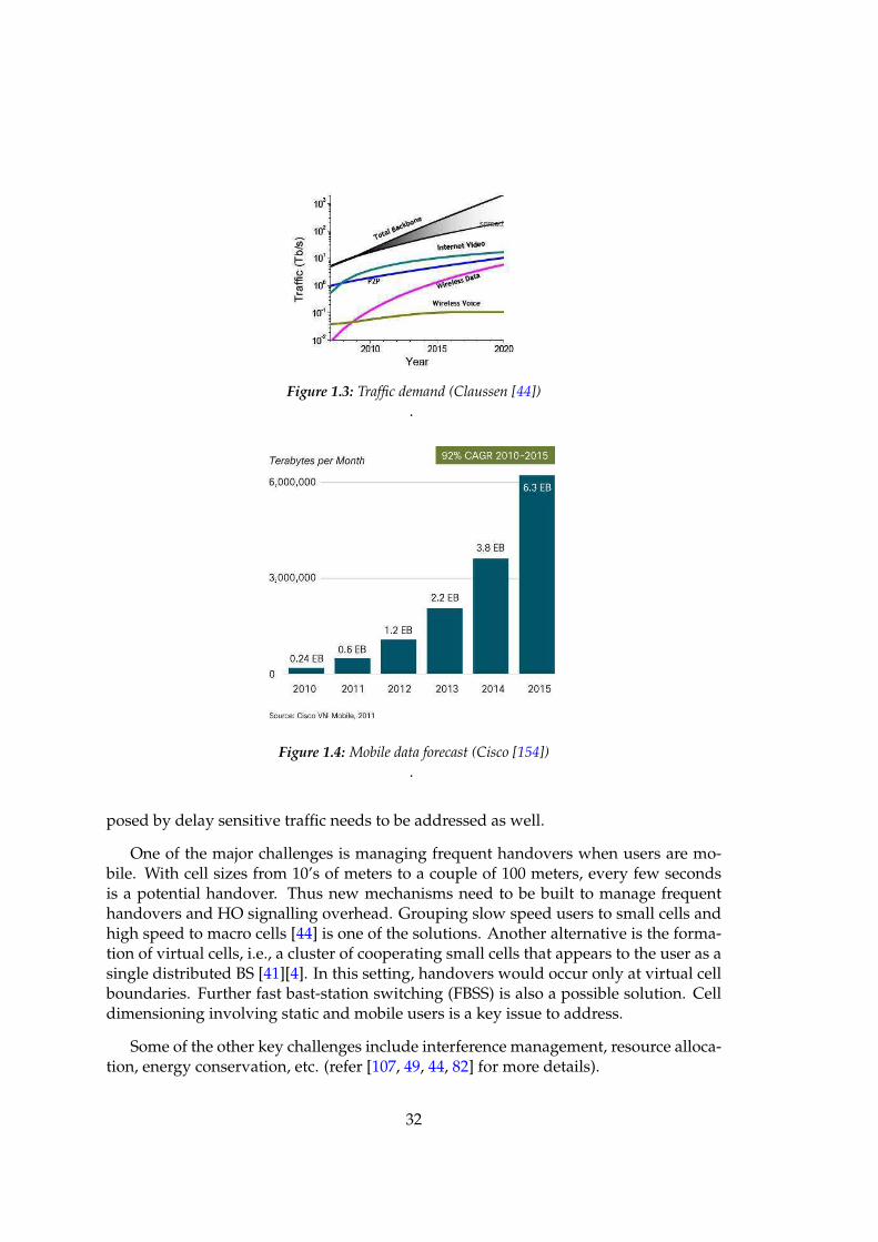
Figure 1.3: Traffic demand (Claussen [44])

.

Figure 1.4: Mobile data forecast (Cisco [154])

.

posed by delay sensitive traffic needs to be addressed as well.

One of the major challenges is managing frequent handovers when users are mo-bile. With cell sizes from 10’s of meters to a couple of 100 meters, every few secondsis a potential handover. Thus new mechanisms need to be built to manage frequenthandovers and HO signalling overhead. Grouping slow speed users to small cells andhigh speed to macro cells [44] is one of the solutions. Another alternative is the forma-tion of virtual cells, i.e., a cluster of cooperating small cells that appears to the user as asingle distributed BS [41][4]. In this setting, handovers would occur only at virtual cellboundaries. Further fast bast-station switching (FBSS) is also a possible solution. Celldimensioning involving static and mobile users is a key issue to address.

Some of the other key challenges include interference management, resource alloca-tion, energy conservation, etc. (refer [107, 49, 44, 82] for more details).

32

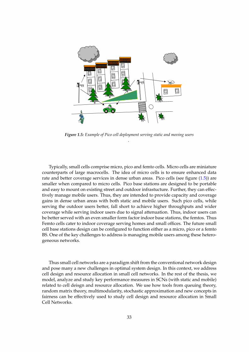
Figure 1.5: Example of Pico cell deployment serving static and moving users

.

Typically, small cells comprise micro, pico and femto cells. Micro cells are miniaturecounterparts of large macrocells. The idea of micro cells is to ensure enhanced datarate and better coverage services in dense urban areas. Pico cells (see figure (1.5)) aresmaller when compared to micro cells. Pico base stations are designed to be portableand easy to mount on existing street and outdoor infrastucture. Further, they can effec-tively manage mobile users. Thus, they are intended to provide capacity and coveragegains in dense urban areas with both static and mobile users. Such pico cells, whileserving the outdoor users better, fall short to achieve higher throughputs and widercoverage while serving indoor users due to signal attenuation. Thus, indoor users canbe better served with an even smaller form factor indoor base stations, the femtos. ThusFemto cells cater to indoor coverage serving homes and small offices. The future smallcell base stations design can be configured to function either as a micro, pico or a femtoBS. One of the key challenges to address is managing mobile users among these hetero-geneous networks.

Thus small cell networks are a paradigm shift from the conventional network designand pose many a new challenges in optimal system design. In this context, we addresscell design and resource allocation in small cell networks. In the rest of the thesis, wemodel, analyze and study key performance measures in SCNs (with static and mobile)related to cell deisgn and resource allocation. We use how tools from queuing theory,random matrix theory, multimodularity, stochastic approximation and new concepts infairness can be effectively used to study cell design and resource allocation in SmallCell Networks.

33

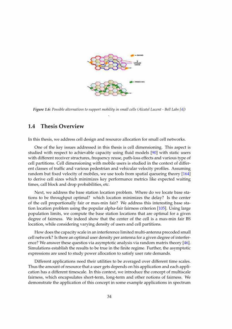
Figure 1.6: Possible alternatives to support mobility in small cells (Alcatel Lucent - Bell Labs [4])

.

1.4 Thesis Overview

In this thesis, we address cell design and resource allocation for small cell networks.

One of the key issues addressed in this thesis is cell dimensioning. This aspect isstudied with respect to achievable capacity using fluid models [90] with static userswith different receiver structures, frequency reuse, path-loss effects and various type ofcell partitions. Cell dimensioning with mobile users is studied in the context of differ-ent classes of traffic and various pedestrian and vehicular velocity profiles. Assumingrandom but fixed velocity of mobiles, we use tools from spatial queueing theory [164]to derive cell sizes which minimizes key performance metrics like expected waitingtimes, call block and drop probabilities, etc.

Next, we address the base station location problem. Where do we locate base sta-tions to be throughput optimal? which location minimizes the delay? Is the centerof the cell proportionally fair or max-min fair? We address this interesting base sta-tion location problem using the popular alpha-fair fairness criterion [105]. Using largepopulation limits, we compute the base station locations that are optimal for a givendegree of fairness. We indeed show that the center of the cell is a max-min fair BSlocation, while considering varying density of users and cell partitions.

How does the capacity scale in an interference limited multi-antenna precoded smallcell network? Is there an optimal user density per antenna for a given degree of interfer-ence? We answer these questios via asymptotic analysis via random matrix theory [46].Simulations establish the results to be true in the finite regime. Further, the asymptoticexpressions are used to study power allocation to satisfy user rate demands.

Different applications need their utilities to be averaged over different time scales.Thus the amount of resource that a user gets depends on his application and each appli-cation has a different timescale. In this context, we introduce the concept of multiscalefairness, which encapsulates short-term, long-term and other notions of fairness. Wedemonstrate the application of this concept in some example applications in spectrum

34

allocation and indoor-outdoor femto cells.

How do we allocate power to satisfy user demands in a multi-cell, heterogeneousnetwork?. We address this problem and propose a stochastic approximation [93] baseduniversal power allocation algorithm. We demonstrate the working of this algorithmfor systems with various degree of co-operation. This self-organizing algorithm fits theparadigm of self organizing small cell networks.

Dense deployment of small cell’s address capacity and coverage holes. But, thesystem load varies over time. Hence, from a greener perspective, one can switch off afraction of base stations via a central control or put a base station in an idle mode viadecentralized control, depending on the load. We derive the structure of this controlusing tools from multimodularity [12].

High speed mobiles are subjected to frequent handovers due to the dimension ofsmall cells during the course of their service. We address this problem of managing highspeed mobility. We propose novel ways of power and resource allocation to managehigh speed users in small cells.

1.5 Tools used in the thesis

In this section, we present a brief overview of the tools used in the thesis. We have usedfluid limits [90] to address cell dimensioning with static users in chapter 2. Fluid lim-its many a times yield explicit expressions for relevant performance measures, whichare tractable and are a good starting point to study complex problems (e.g, cell dimen-sioning). Further they reduce the simulation overhead. Similar tools are also used inchapter 4 to address the base station placement problem.

Fluid limits are asymptotic limits and hence are valid when some underlying quan-tities tend to infinity. For example when the user density or base station density in-creases to infinity. Alternatively, queueing tools are useful when asymptotics are notvalid. In chapter 3, we use queueing tools to derive cell dimensions that optimize ser-vice times, waiting times, call block and drop probabilities, while considering mobileusers. Explicit expressions for various performance metrics can be easily found in mostof the books on queueing theory, e. g., [164] and can be straightaway used if a systemcan be modeled as a certain type of a queue.

To analyze capacity scaling and per antenna user density that can be supported ininterference limited multicell precoded systems in chapter 5, we have used randommatrix theory [149, 46]. Most often, the limiting spectral distribution of these largerandom matrices, representative of the system under consideration can be expressedexplicitly by the popular Stieltjes or other transforms. The asymptotic results obtainedvia such an approach has been shown to be quite effective even in the finite regime.

For the problem of deriving the structure of the control policy for base station ac-tivation in chapter 6, we have used tools from Multimodularity. Multimodularity ad-dresses convex functions over integer spaces and if applied to systems whose cost func-

35

tion evolves in a max-plus algebra, the axioms of Multimodularity can be proven andthe result is a simple well structured policy. This tool, introduced in [75] has been usedto address many problems in admission control, routing and other applications [12].

Fairness comes at the cost of efficiency. But, users can demand the same QoS ir-respective of their location w.r.t the serving base station. So, the resource allocationpolicies at the base stations cannot always be selfish to maximize their own revenue.To keep the user satisfied, they have to sometimes maximize the utility of the weakestuser. So, it is necessary to be fair on many counts (global, proportional, delay minimiz-ing, max-min, etc., ). These different notions of fairness are encapsulated in the conceptof alpha fairness [105]. Further, different applications need the utilties to be averagedover different time scales. With this view, the concept of alpha fairness in conjunctionwith traffic type and averaging durations has been used to come up with new fairnessconcepts; the T-scale and multiscale fairness in chapter 7. The concept of alpha fairnessis also used in fair location of base stations chapter 4.

Stochastic approximation (e.g., [93]) analysis are powerful and are used extensivelyin a variety of applications with iterative algorithms. They are handful in obtainingthe transient as well as steady state behaviour of the iterative algorithms. Ordinarydifferential equation (ODE) approach is a popular one while studying the stochasticapproximation based algorithms. In this approach, either the iterative algorithm is ap-proximated by the trajectory of an appropriate ODE or the time asymptotic limits ofan algorithm are obtained via the attractors of a ODE. In chapter 8, we proposed auniversal (one which works in variety of systems) power allocation algorithm, whichwhile running independently and simultaneosly at all the base stations of the network,assymptotically satisfies the demands of all the users of the network. We obtained theanalysis of the proposed algorithm via the ODE analysis. The same chapter also usesGame theoretic tools to obtain the demand satisfying power profile as a nash equilib-rium of an appropriate game.

These analysis are used for obtaining the For our power allocation problem to sat-isfy user demands with base station power constraints i we have proposed a stochas-tic approximation based universal algorithm which can work in a variety of systems.This algorithm converges to a power profile, which is the zero of the function beingaddressed in this case. Also, specific to this problem, we have used a simple game the-oretic framework [11] to formulate the problem and as has been a popular approach,we use an ordinary differential equation (ODE) [93] approach to analyze the algorithm.

For the purpose of simulations, we have used MATLAB and MAPLE extensively.Especially MAPLE is a favorite tool to check if explicit expressions are possible forseemingly difficult integrals and other mathematical functions. We further propose touse the LTE system level simulator [161] to validate some of the ideas and algorithmsdeveloped during the course of our thesis.

36

1.6 Organization and Contributions

This dissertation focuses on cell design and resource allocation for small cell networks.The chapters are organized in two parts. The first part deals with cell design, while thesecond part discusses resource allocation. Our main contributions and the outline ofthe chapters content are the following

Part A: Cell design and dimensioning

1. Cell dimensioning with static users: A fluid perspective [115].

2. Cell dimensioning with moving users: A Spatial queuing approach [89], [119],[118].

3. Where to locate the base station?: A large population perspective [116].

4. Capacity scaling and per-antenna user density in multi-antenna precoded net-works: A random matrix approach [117].

5. BS activation control for green networking: A multimodularity approach [120].

Part B: Resource allocation

1. Multiscale Fairness and its Application to Resource Allocation in Wireless Net-works [8], [10], [9], [114].

2. Satisfying Demands in a Multicellular Network: A Universal Power AllocationAlgorithm [121].

In Introduction 1, we provided a brief overview of the generation of wireless net-works, the need for small cells, an overview of the thesis, tools used to address prob-lems in the thesis and chapter highlights.

In Chapter 2, we present a systematic study of the uplink capacity and coverage ofpico-cell wireless networks. Both the one dimensional as well as the two dimensionalcases are investigated. Our goal is to compute the size of pico-cells that maximizes thespatial throughput density. To achieve this goal, we consider fluid models that allow usto obtain explicit expressions for the interference and the total received power at a basestation. We study the impact of various parameters on the performance: the path lossfactor, the spatial reuse factor and the receiver structure (matched filter or multiuserdetector).

In Chapter 3, we characterize the performance of Picocell networks in presence ofmoving users. We model various traffic types between base-stations and mobiles asdifferent types of queues. We derive explicit expressions for expected waiting time,service time and drop/block probabilities for both fixed as well as random velocity ofmobiles. We obtain (approximate) closed form expressions for optimal cell size whenthe velocity variations of the mobiles is small for both non-elastic as well as elastictraffic. We conclude from the study that, if the expected call duration is long enough,the optimal cell size depends mainly on the velocity profile of the mobiles, its mean and

37

variance. It is independent of the traffic type or duration of the calls. Further, for anyfixed power of transmission, there exists a maximum velocity beyond which successfulcommunication is not possible. This maximum possible velocity increases with thepower of transmission. Also, for any given power, the optimal cell size increases wheneither the mean or the variance of the mobile velocity increases.

In Chapter 4, we address the problem of fair assignment of base station locationsin a cellular network. We use the generalized α-fairness criterion, which encompassesthe different notions of fairness: that of global, proportional, harmonic or max-minfairness in our study. We derive explicit expression for α-fair BS locations under ’largepopulation’ limits in the case of simple 1D models. We show analytically that as αincreases asymptotically, the optimal location for a single BS converges to the center ofthe cell. We validate our analysis via numerical examples. We further study throughputachievable as a function of α-fair BS placement, path-loss factor β and noise variance σ2

via numerical examples. We also briefly address the problem of optimal placement oftwo base stations and obtain similar conclusions.

In Chapter 5, we study precoded MIMO based small cell networks. We derive thetheoretical sum-rate capacity, when multi-antenna base stations transmit precoded in-formation to its multiple single-antenna users in the presence of inter-cell interferencefrom neighboring cells. Due to an interference limited scenario, increasing the num-ber of antennas at the base stations does not yield necessarily a linear increase of thecapacity. We assess exactly the effect of multi-cell interference on the capacity gain fora given interference level. We use recent tools from random matrix theory to obtainthe ergodic sum-rate capacity, as the number of antennas at the base station, numberof users grow large. Simulations confirm the theoretical claims and also indicate thatin most scenarios the asymptotic derivations applied to a finite number of users givegood approximations of the actual ergodic sum-rate capacity.

In recent years there has been an increasing awareness that the deployment as wellas utilization of new information technology may have some negative ecological im-pact. This includes awareness to energy consumption which could have negative con-sequences on the environment. In recent years, it was suggested to increase energysaving by deactivating base stations during periods in which the traffic is expected tobe low. In Chapter 6, we study the optimal deactivation policies, using recent toolsfrom Multimodularity (which is the analog concept of convexity in optimization overintegers). We consider two scenarios: In the first case, a central control derives the opti-mal open loop policies so as to maximize the expected throughput of the system giventhat at least a certain percentage of Base stations are deactivated (switched OFF). In thesecond case, we derive optimal open loop polices, which each base station can employin a decentralized manner to minimize the average buffer occupancy cost when thefraction of time for which the BS station is deactivated (idle mode) is lower bounded.In both the cases, we show that the cost structure is Multimodular and characterize thestructure of optimal policies.

Fair resource allocation is usually studied in a static context, in which a fixed amountof resources is to be shared. In dynamic resource allocation one usually tries to assign

38

resources instantaneously so that the average share of each user is split fairly. The exactdefinition of the average share may depend on the application, as different applica-tions may require averaging over different time periods or time scales. In Chapter 7,we study dynamic resource allocation in wireless networks. Our main contributionis to introduce new refined definitions of fairness that take into account the time overwhich one averages the performance measures. We examine how the constraints on theaveraging durations impact the amount of resources that each user gets.

Power allocation to satisfy user demands in the presence of large number of inter-ferers in a multicellular network is a challenging task. Further, the power to be allo-cated depends upon the system architecture, for example upon components like cod-ing, modulation, transmit precoder, rate allocation algorithms, available knowledge ofthe interfering channels, etc. This calls for an algorithm via which each base station inthe network can simultaneously allocate power to their respective users so as to meettheir demands (when they are within the achievable limits), using whatever informa-tion is available of the other users. In Chapter 8, we propose one such algorithm whichin fact is universal: the proposed algorithm works from a fully co-operative settingto almost no co-operation and or for any configuration of modulation, rate allocation,etc. schemes. The algorithm asymptotically satisfies the user demands, running simul-taneously and independently within a given total power budget at each base station.Further, it requires minimal information to achieve this: every base station needs toknow its own users demands, its total power constraint and the transmission rates al-located to its users in every time slot. We formulate the power allocation problem ina system specific game theoretic setting, define system specific capacity region and an-alyze the proposed algorithm using ordinary differential equation (ODE) framework.Simulations confirm the effectiveness of the proposed algorithm.

Summary and future research directions are discussed in Conclusion 9. A list ofpublications during the course of the thesis is available in Publications 9

39

Part II

Cell Design

41

Chapter 2

Cell Dimensioning with StaticUsers, a fluid perspective

Contents2.1 Introduction . . . . . . . . . . . . . . . . . . . . . . . . . . . . . . . . . 43

2.2 Received Power computation . . . . . . . . . . . . . . . . . . . . . . . . 45

2.3 Throughput . . . . . . . . . . . . . . . . . . . . . . . . . . . . . . . . . . 47

2.4 Impact of cell size on throughput . . . . . . . . . . . . . . . . . . . . . 51

2.5 Indoor analysis . . . . . . . . . . . . . . . . . . . . . . . . . . . . . . . . 53

2.6 Dimension 2 . . . . . . . . . . . . . . . . . . . . . . . . . . . . . . . . . . 54

2.7 Coverage and capacity . . . . . . . . . . . . . . . . . . . . . . . . . . . . 59

2.8 Conclusions and future perspectives . . . . . . . . . . . . . . . . . . . 62

2.9 Publications . . . . . . . . . . . . . . . . . . . . . . . . . . . . . . . . . . 63

2.1 Introduction

In a Small cell, the shorter transmission distance coupled with lower transmit power,enhances both capacity as well as the Signal to Interference Noise Ratio (SINR) achiev-able within the cell. But, a designer or a system architect would like to answer questionssuch as: What is the optimum number of cells that one would want to divide the macro-cell?, What is the optimum cell size which maximizes the throughput achievable at aSmall cell?. Does the receiver configuration matter? How is throughput affected whenone moves from a deployment of Small cells on a street (1D) to a deployment in a officespace or shopping mall (2D)?. What if the entire cell is located indoors? What happensif the Small cell BS is within the building or located outside? What is the implication offrequency reuse on the throughput achievable?

In this chapter, we try to address several of these questions. In particular, we deriveexplicit expressions for the up-link (UL) SINR and throughput for simple 1D and 2D

43

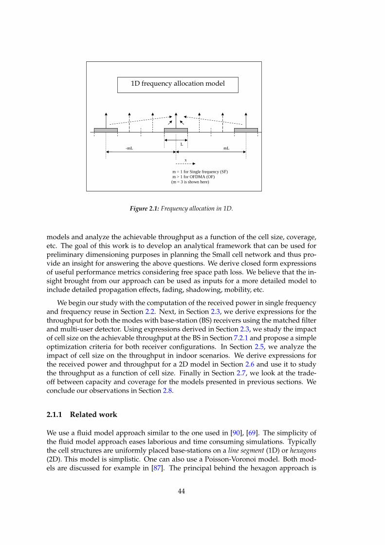
L mL -mL

m = 1 for Single frequency (SF) m > 1 for OFDMA (OF) (m = 3 is shown here)

x

Figure 2.1: Frequency allocation in 1D.

models and analyze the achievable throughput as a function of the cell size, coverage,etc. The goal of this work is to develop an analytical framework that can be used forpreliminary dimensioning purposes in planning the Small cell network and thus pro-vide an insight for answering the above questions. We derive closed form expressionsof useful performance metrics considering free space path loss. We believe that the in-sight brought from our approach can be used as inputs for a more detailed model toinclude detailed propagation effects, fading, shadowing, mobility, etc.

We begin our study with the computation of the received power in single frequencyand frequency reuse in Section 2.2. Next, in Section 2.3, we derive expressions for thethroughput for both the modes with base-station (BS) receivers using the matched filterand multi-user detector. Using expressions derived in Section 2.3, we study the impactof cell size on the achievable throughput at the BS in Section 7.2.1 and propose a simpleoptimization criteria for both receiver configurations. In Section 2.5, we analyze theimpact of cell size on the throughput in indoor scenarios. We derive expressions forthe received power and throughput for a 2D model in Section 2.6 and use it to studythe throughput as a function of cell size. Finally in Section 2.7, we look at the trade-off between capacity and coverage for the models presented in previous sections. Weconclude our observations in Section 2.8.

2.1.1 Related work

We use a fluid model approach similar to the one used in [90], [69]. The simplicity ofthe fluid model approach eases laborious and time consuming simulations. Typicallythe cell structures are uniformly placed base-stations on a line segment (1D) or hexagons(2D). This model is simplistic. One can also use a Poisson-Voronoi model. Both mod-els are discussed for example in [87]. The principal behind the hexagon approach is

44

to construct a disc with an equivalent area similar to the hexagon (OR hexagons of in-terest). While in the Poisson-Voronoi model, the base station locations and cell sizesare random. These two are extreme and complementary architectures: The hexagonalmodel represents perfectly structured networks, whereas the Poisson-Voronoi modeltakes into account irregularities of real networks in a statistical way. We shall treat indetail the hexagonal model in this work.

An alternative fluid model has been introduced in [31, 30] to study the performanceand optimal cell size for CDMA networks. The model includes fading, and the fluidlimits are those obtained when the density of mobiles become large. The main toolthere has been random matrix theory. The approach in [31, 30] requires complete ho-mogeneity within each cell: the gain from a mobile to a base station does not depend onthe location of the mobile. In contrast, in our work, we take into account the detailedimpact of the distance on the channel gains. In [135] the authors address a relatedproblem of optimizing the spectral efficiency of cellular indoor wireless networks byadjusting the location and power of the base-stations. They apply both continuous andcombinatorial approaches to find a solution to the optimization problem.

2.2 Received Power computation

We compute the total power received at the base station for single frequency and fre-quency reuse modes as a function of the cell size. The single frequency or frequencyreuse modes can employ single carrier or OFDM modulation for transmission.

2.2.1 Single frequency (SF)

Assume a single frequency deployment. There is a uniform density of mobiles onthe line L = ((−∞, 0), (∞, 0), each transmitting at a unit power (similar to the fluidmodel approach used in [90], [31]). There are base stations (BS) located at (nL, 1), n =...,−1, 0, 1, .... Since we consider Small cells, we explicitly include in the geometricmodel the vertical distance (normalized to one) of the base station (which could benegligible in large cells). Let α represent the attenuation factor or path loss factor inthe given wireless environment (for practical values of alpha one can refer for ex. to[123]). Thus the power received at the BS from a mobile at a distance of x is equal to(1 + x2)−α/2.

Denote β1 = (α − 1)/2 and β2 = (α + 1)/2. The total power received at the BS is

Ptotbs =

∫ ∞

−∞(1 + x2)−α/2dx =

√πΓ(β1)

Γ(α/2)(2.1)

In particular, we have in Table 4.1 explicit expressions for some integer valued α’s:

45

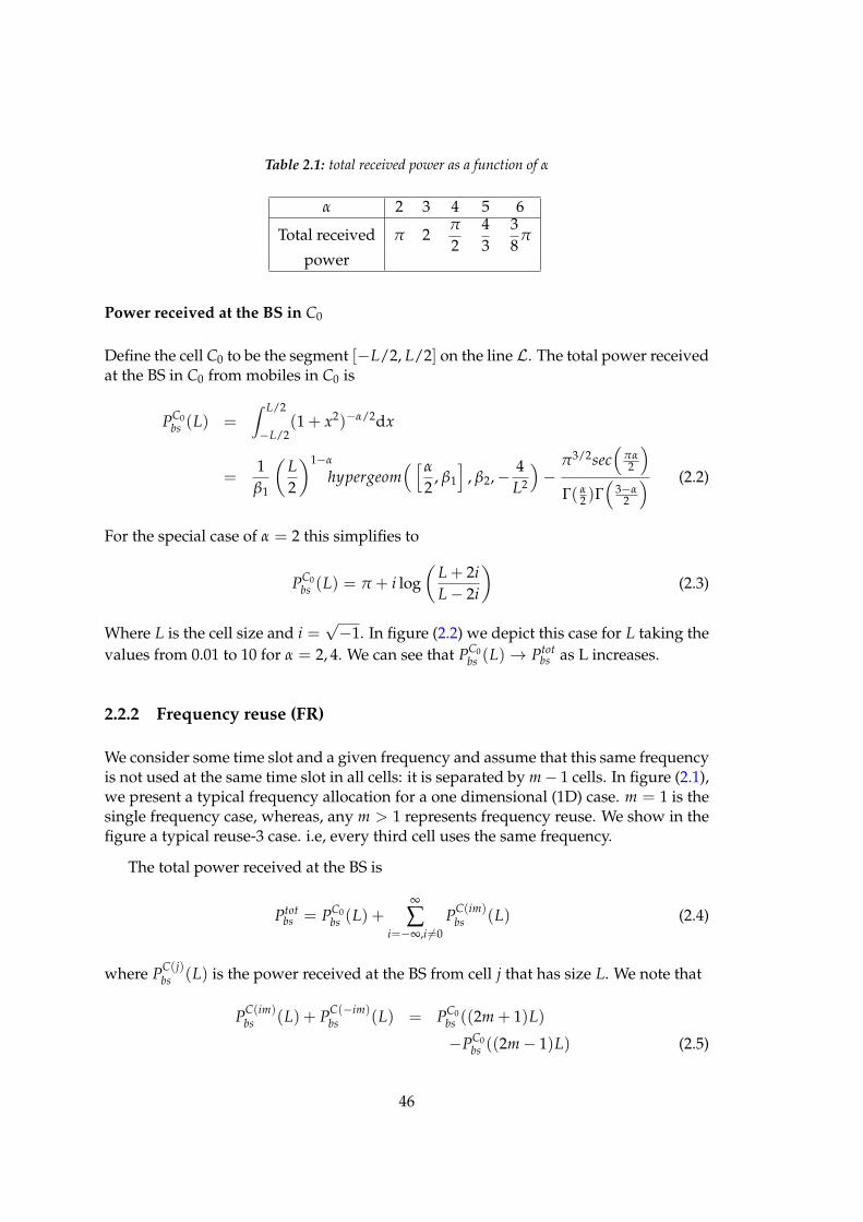
Table 2.1: total received power as a function of α

α 2 3 4 5 6

Total received π 2π

243

38

π

power

Power received at the BS in C0

Define the cell C0 to be the segment [−L/2, L/2] on the line L. The total power receivedat the BS in C0 from mobiles in C0 is

PC0bs (L) =

∫ L/2

−L/2(1 + x2)−α/2dx

=1β1

(

L

2

)1−α

hypergeom( [α

2, β1

]

, β2,− 4L2

)

−π3/2sec

(

πα2

)

Γ( α2 )Γ(

3−α2

) (2.2)

For the special case of α = 2 this simplifies to

PC0bs (L) = π + i log

(

L + 2i

L − 2i

)

(2.3)

Where L is the cell size and i =√−1. In figure (2.2) we depict this case for L taking the

values from 0.01 to 10 for α = 2, 4. We can see that PC0bs (L) → Ptot

bs as L increases.

2.2.2 Frequency reuse (FR)

We consider some time slot and a given frequency and assume that this same frequencyis not used at the same time slot in all cells: it is separated by m − 1 cells. In figure (2.1),we present a typical frequency allocation for a one dimensional (1D) case. m = 1 is thesingle frequency case, whereas, any m > 1 represents frequency reuse. We show in thefigure a typical reuse-3 case. i.e, every third cell uses the same frequency.

The total power received at the BS is

Ptotbs = PC0

bs (L) +∞

∑i=−∞,i 6=0

PC(im)bs (L) (2.4)

where PC(j)bs (L) is the power received at the BS from cell j that has size L. We note that

PC(im)bs (L) + P

C(−im)bs (L) = PC0

bs ((2m + 1)L)

−PC0bs ((2m − 1)L) (2.5)

46

2.3 Throughput

We compute the total achievable throughput at a cell in the case where the BS receiveruses a matched filter or employs a multi-user detection scheme like successive interfer-ence cancellation.

2.3.1 Matched filter (MF)

We model the power received at BS in cell C0 from a mobile at x as the total powerreceived from [x, x + dx], i.e. dP(x) = (1 + x2)−α/2dx. We use the Shannon capacityto compute the throughput while treating the interferences from all other mobiles atthe same frequency and time as noise. Using a detection scheme based on the matchedfilter, the achievable throughput from the mobile at x is

dθ(x) = log(

1 +dP(x)

σ2 + Ptotbs

)

where, σ2 is the noise power.

Since the quantitydP(x)

Ptotbs

<< 1, we use log(1 + x) ≈ x and rewrite

dθ(x) =dP(x)

σ2 + Ptotbs

(2.6)

Hence the total throughput at the cell is given by

Θ(L) =

∫ L/2−L/2 dP(x)dx

σ2 + Ptotbs

=PC0

bs (L)

σ2 + Ptotbs

. (2.7)

and the throughput density is given by

ΨMF(L) =ΘC

L=

PC0bs (L)/L

σ2 + Ptotbs

. (2.8)

Let L∗ denote the cell size which maximizes the throughput density.Lemma 2.3.2. In the case of the matched filter, the throughput density is maximized by takingbase stations as dense as possible. i.e, L∗ → 0.

Proof : From equation (2.8),

L∗ = arg maxL

PC0bs (L)/L

(

σ2 + Ptotbs

)

= arg maxL

PC0bs (L)/L

= arg maxL

(

1L

∫ L

0(1 + x2)

−α2 dx

)

47

as σ2 and Ptotbs are independent of L. Clearly,

∫ L

01

−α2 dx >

∫ L

0(1 + x2)

−α2 dx >

∫ L

0(1 + L2)

−α2 dx

and hence,

1 >PC0

bs (L)

L> (1 + L2)

−α2 .

From the above, it is easy to see that,

PC0bs (L)

L< 1 if L > 0,

PC0bs (L)

L→ 1 as L → 0.

And thus, L∗ = 0.

2.3.3 Multi-user detection (MD)

We assume that all the signal received at BS in cell C0 from mobiles out of C0 are consid-ered noise; however within C0, some multi-user detection scheme that maximizes thecell throughput is used. For example, successive interference cancellation is assumed.Then the SINR is given by

SINR =PC0

bs (L)

σ2 + Ptotbs − PC0

bs (L). (2.9)

and the throughput achievable using the Shannon capacity limit with the multi-userdetection constraint [153]

Θ(L) = log (1 + SINR) (2.10)

and the throughput density is

ΨMD(L) =Θ

L=

log (1 + SINRC)

L(2.11)

Lemma 2.3.4. In the case of multi-user detection, the cell size which maximizes throughputdensity is such that L∗

> 0

Proof : From equation (2.11),

L∗ = arg maxL

1L

log

(

1 +PC0

bs (L)


bs (L)

)

(2.12)

Let σ2 + Ptotbs = K. By monotonicity of log function,

L∗ = arg maxL

(

K

K − PC0bs (L)

) 1L

.

48

Clearly,L > PC0

bs (L) > L(1 + L2)−α2

and hence,(

K

K − L(1 + L2)−α2

) 1L

>

(

K

K − PC0BS(L)

) 1L

>

(

K

K − L

) 1L

From the above, it is easy to see that

(

K

K − PC0BS(L)

) 1L

> 1 if L > 0,

(

K

K − PC0BS(L)

) 1L

→ 1 as L → 0.

Thus there is an L∗> 0, which maximizes the throughput density.

Computation of L∗: By virtue of Lemma 2.3.4, L∗> 0, i.e., the maximizer is not

at the boundary point and the objective function is clearly a differentiable function.Hence, the cell size which maximizes the throughput density is a zero of the derivativedΨMD/dL and hence is a zero of

Ω(L∗; α, σ2) = 0 (2.13)

where

Ω(L; α, σ2) := L

(

1 +L2

4

)

−α2

−(


bs

)

log

(

σ2 + Ptotbs


bs

)

Finding an explicit expression for L∗ is not easy. We outline a simple procedure tocompute L∗ iteratively.

Lk+1 = Lk + ǫ Ω(Lk; α, σ2) (2.14)

L0 > 0 is the initial value for the first iteration and L∗ is the converged value. One canconfirm the above iteration has converged whenever the error |Lk+1 − Lk| < µ for somesmall enough positive constant µ.

For example, with α = 2, σ2 = 1, L0 = 0.1 and ǫ = 0.1, we converge to L∗ = 0.85 in150 iterations. This matches with the optimal (max) value for the curve labeled SF_MDin figure (2.5).

Asymptotic Approximations for L∗ in Small cells: We derive approximations forL∗ as the path-loss factor α converges to 0 or to ∞. We recall from equation (2.11),

L∗ = arg maxL∈[0,Lmax ]

1L

log

(

1 +PC0

bs (L)


bs (L)

)

.

49

In the above, Lmax represents the maximum cell size that we can design. Since we aredealing with Small cells Lmax itself is a small number and hence PC0

bs (L) ≪ Ptotbs . So we

can use the approximation log(1 + x) ≈ x and re-write

L∗ = arg maxL∈[0,Lmax ]

1L

(

PC0bs (L)

Kα − PC0bs (L)

)

,

where Kα := σ2 + Ptotbs .

For large values of α : By bounded convergence theorem as α → ∞, PC0bs (L)− L(1 +

L2)−α/2 → 0. Therefore for large values of α,

L∗ ≈ arg maxL

1L

(

L(1 + L2)−α/2

Kα − L(1 + L2)−α/2

)

or L∗ approximately solves

d(

(1+L2)−α/2

Kα−L(1+L2)−α/2

)

dL

∣

∣

∣

∣

∣

∣

L=L∗

= 0.

Solving this yields

L∗ ≈ 1αKα

for large values of α. (2.15)

For small values of α : By bounded convergence theorem again as α → 0, PC0bs (L) → L.

Therefore, L∗ ≈ arg maxL

(

1Kα − L

)

for small values of α. Hence

L∗ ≈ Lmax for small values of α. (2.16)

In figure (2.9), we plot L∗ as a function of α computed using equations (2.15), (2.16)and compare it with the value of L∗ computed via numerical simulations. We see thatthe numerically evaluated values lie within the two bounds. Also, for smaller valuesof α, the simulation results are closer to the α small bound and for larger values, thesimulation results are closer to the α large bound.

2.3.5 Comments on the fluid approach

So far we have been working with a fluid model which had the advantage (over a moredetailed discrete stochastic model) of being sufficiently simple to allow us to obtainexplicit expressions for performance measures related to the system capacity. We nowaddress the question of the validity of the fluid approximation: can we estimate whatthese expressions say on the original discrete system? To address the question we firstdefine our stochastic model. We assume a Poisson arrival process with constant inten-sity.

50

Assume that mobiles are located according to a uniform Poisson point process X =Xi with intensity λ which we normalize to one unit. Nx(A) denotes the number ofpoints of the process X in a set A. Consider first the single frequency setting of Section

2.2.1. Then the total power received at the BS is given by∞

∑i=−∞

(1 + X2i )

−α/2 and its

expectation equals precisely to∫ ∞

−∞(1 + x2)−α/2dx, for which equation (2.1) provides

an explicit expression (for integer α’s).

The power and the interferences received at the BS according to the fluid approxi-mation are thus precisely the expectation of those corresponding to the discrete model.In particular, the remaining equations of Section 2.2.1 also hold for the expectations ofthe corresponding objects in the discrete model.

The total throughput of the cell is then given by equation (2.7) and its expectationsatisfies

E[Θ(L)] = E[PC0bs (L)]E

[

1σ2 + Ptot

bs

]

≥ E[PC0bs (L)]

σ2 + E[Ptotbs ]

where the first equality follows from the independence properties due to the Poissonassumption on the location of mobiles, and the last step follows by Jensen’s inequality.We conclude that the throughput results of the fluid model provide lower bounds tothose of the discrete model.

2.4 Impact of cell size on throughput

In this section, we use the expressions obtained in the previous sections to study theimpact of the cell size on throughput. This analysis will allow us to optimize the cell sizefor the different modes and receiver schemes considered. We perform the throughputanalysis via some numerical examples.

2.4.1 Numerical results

In figure (2.4), we plot the total achievable throughput in C0 as a function of the cellsize L which is obtained using equation (2.7), (2.10). We consider two cases, the firstcase when all the cells deployed use the same frequency and the second case where weuse a reuse factor of 3. i.e, every third cell uses the same frequency. We compute thethroughput for the matched filter as well as the multi-user detection scheme in bothsingle frequency and frequency reuse. We plot the throughput as a function of L infigure (2.4) for α = 2. As expected, the throughput increases with L and multi-userdetection performs better than the matched filter.

Next, we look at the total throughput density achievable in C0 as a function of L.For the single frequency case, when the BS receiver uses a matched filter (SF_MF), wenote that the numerator in the throughput density (equation (2.8)) depends on L; it

51

represents the useful power density received. By Lemma 1, we know that the optimalcell size that maximizes the throughput density, L∗ → 0. Figure (2.3) plots the powerdensity as a function of L. We observe that the power density decreases with L andis maximum when L∗ → 0. Thus we can conclude that the throughput density is maxi-mized by taking base stations as dense as possible for a BS receiver which uses a matchedfilter. With frequency reuse, the throughput density also depends upon L via the totalreceived power (see equations (2.4), (2.8)). Hence, we directly compute the throughputdensity in this case.

As before, we consider the two cases described previously. We plot the through-put density as a function of L in figure (2.5), for α = 2. We also plot the throughputdensity for a single frequency with a matched filter (SF_MF), frequency reuse with amatched filter (FR_MF), single frequency with multi-user detection (SF_MD) and fre-quency reuse with multi-user detection (FR_MD) in the same figure.

By Lemma 2, we would expect that the cell size which maximizes the throughputdensity, L∗

> 0, for the BS receiver which employs multi-user detection. From thenumerical example we conducted (figure (2.5) ), we indeed see that L∗

> 0 and infact, there is a unique optimal L for a certain frequency reuse which maximizes thethroughput density. The effect is more pronounced in the frequency reuse case. Also,we achieve a higher throughput density for smaller cell sizes for the more practical caseof α = 4 in contrast to α = 2.

2.4.2 Optimizing the cell size

Matched filter: We see from figure (2.5) that in the matched filter case, the throughputdensity is maximized for smaller cell sizes. However there is a cost for deploying basestations. So it is more natural to pose the problem of maximizing

J(L) =1L(c1Θ(L)− c2) (2.17)

where c1/L is the revenue per throughput density and c2 is the cost of each BS.

We note from figure (2.10)

that the throughput density is not sensitive at all to the reuse parameter m in thematched filter case. (the cell size, L∗, which maximizes the throughput density is always equalto the smallest L considered in the numerical analysis). Also, note that the optimization isover the integers and L is typically not larger than a few hundreds. This allows one tosolve the optimization problem in a very short time even if exhaustive search is used.

Multi-user detection: For a BS which employs multi-user detection, we observefrom numerical analysis (see figure (2.10)) that L∗ decreases as the reuse factor m in-creases. So, as the reuse factor increases, one would prefer to reduce the cell size inorder to maximize throughput density (densify base stations). However, this increasesdeployment costs. Hence, our problem is to find an optimal cell size which balancesthe throughput and deployment costs over the reuse factors of interest. Assuming that

52

the deployment cost is proportional to the frequency reuse factor m, we can formulatethis problem as:

J(L, m) =1L(c1Θ(L)− c2 − mc3) (2.18)

as before, c1/L is the revenue per throughput density and c2 is the cost of each BS. Theadditional cost mc3 is incurred due to reuse co-ordination where m is the reuse factorand c3 is the cost per reuse.

2.5 Indoor analysis

2.5.1 BS located inside the building

Next, we consider the cell of interest to be enclosed within a wall. All the interferers arelocated outside of the wall. We use our earlier received power and throughput compu-tation to analyze the performance of the desired cell for both the matched filter as wellas the multi-user detection schemes. Here again, we consider single frequency as wellas frequency reuse, first in the 1D case. We add to the gain, a constant multiplicationterm to take into account the attenuation due to penetration through walls (refer [131],[1], [168] for some example values).

Thus the throughput density equations (2.8) and (2.11) change as

ΨMF(L) =PC0

bs (L)/L

σ2 + ηPtotbs + (1 − η)PC0

bs (L).

and

ΨMD(L) =1L

log

(

1 +PC0

bs (L)

σ2 + η(Ptotbs − PC0

bs (L))

)

, where η is the wall attenuation factor .

We plot the numerical results in figure (2.7) for attenuation η = 12dB

Observations:

• When the interference is attenuated, there does not exist an optimal cell sizewhich maximizes the throughput density for both the matched filter as well asmulti-user detection schemes in single frequency and frequency reuse respec-tively.

• Throughput density increases with path-loss α.

• Throughput density increases with attenuation η.

53

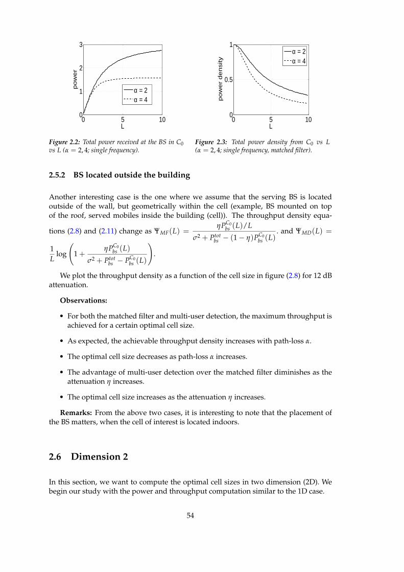
0 5 100

1

2

3

L

po

we

r

α = 2α = 4

Figure 2.2: Total power received at the BS in C0vs L (α = 2, 4; single frequency).

0 5 100

0.5

1

L

po

we

r d

en

sity

α = 2α = 4

Figure 2.3: Total power density from C0 vs L(α = 2, 4; single frequency, matched filter).

2.5.2 BS located outside the building

Another interesting case is the one where we assume that the serving BS is locatedoutside of the wall, but geometrically within the cell (example, BS mounted on topof the roof, served mobiles inside the building (cell)). The throughput density equa-

tions (2.8) and (2.11) change as ΨMF(L) =ηPC0

bs (L)/L

σ2 + Ptotbs − (1 − η)PC0

bs (L). and ΨMD(L) =

1L

log

(

1 +ηPC0

bs (L)


bs (L)

)

.

We plot the throughput density as a function of the cell size in figure (2.8) for 12 dBattenuation.

Observations:

• For both the matched filter and multi-user detection, the maximum throughput isachieved for a certain optimal cell size.

• As expected, the achievable throughput density increases with path-loss α.

• The optimal cell size decreases as path-loss α increases.

• The advantage of multi-user detection over the matched filter diminishes as theattenuation η increases.

• The optimal cell size increases as the attenuation η increases.

Remarks: From the above two cases, it is interesting to note that the placement ofthe BS matters, when the cell of interest is located indoors.

2.6 Dimension 2

In this section, we want to compute the optimal cell sizes in two dimension (2D). Webegin our study with the power and throughput computation similar to the 1D case.

54

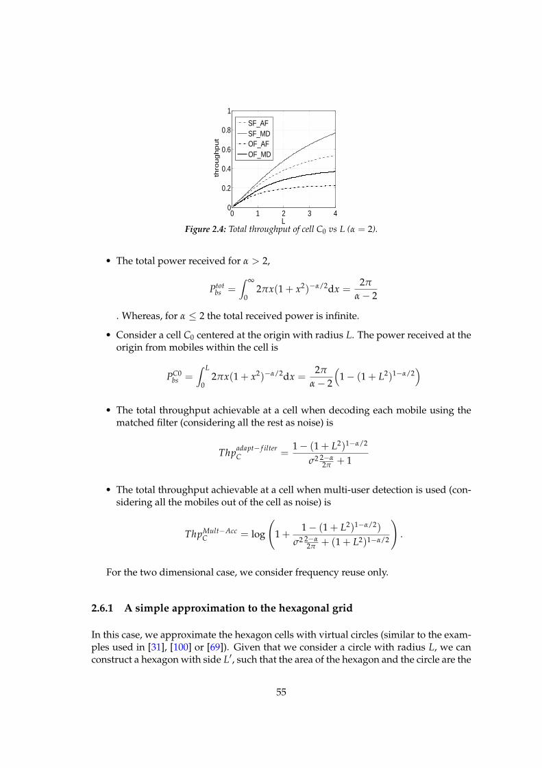
0 1 2 3 40

0.2

0.4

0.6

0.8

1

Lth

roughput

SF_AFSF_MDOF_AFOF_MD

Figure 2.4: Total throughput of cell C0 vs L (α = 2).

• The total power received for α > 2,

Ptotbs =

∫ ∞

02πx(1 + x2)−α/2dx =

2π

α − 2

. Whereas, for α ≤ 2 the total received power is infinite.

• Consider a cell C0 centered at the origin with radius L. The power received at theorigin from mobiles within the cell is

PC0bs =

∫ L

02πx(1 + x2)−α/2dx =

2π

α − 2

(

1 − (1 + L2)1−α/2)

• The total throughput achievable at a cell when decoding each mobile using thematched filter (considering all the rest as noise) is

Thpadapt− f ilterC =

1 − (1 + L2)1−α/2

σ2 2−α2π + 1

• The total throughput achievable at a cell when multi-user detection is used (con-sidering all the mobiles out of the cell as noise) is

ThpMult−AccC = log

(

1 +1 − (1 + L2)1−α/2)

σ2 2−α2π + (1 + L2)1−α/2

)

.

For the two dimensional case, we consider frequency reuse only.

2.6.1 A simple approximation to the hexagonal grid

In this case, we approximate the hexagon cells with virtual circles (similar to the exam-ples used in [31], [100] or [69]). Given that we consider a circle with radius L, we canconstruct a hexagon with side L′, such that the area of the hexagon and the circle are the

55

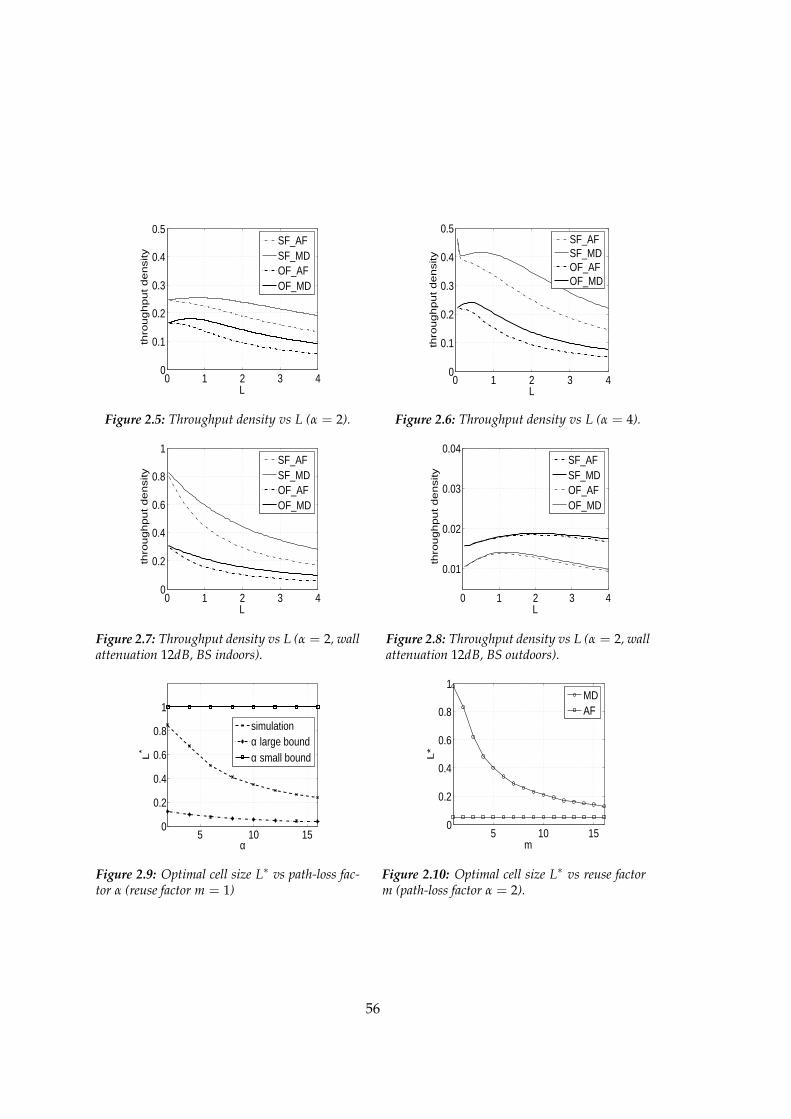
0 1 2 3 40

0.1

0.2

0.3

0.4

0.5

L

thro

ughput density


Figure 2.5: Throughput density vs L (α = 2).

0 1 2 3 40

0.1

0.2

0.3

0.4

0.5

L

thro

ughput density


Figure 2.6: Throughput density vs L (α = 4).

0 1 2 3 40

0.2

0.4

0.6

0.8

1

L

thro

ughput density


Figure 2.7: Throughput density vs L (α = 2, wallattenuation 12dB, BS indoors).

0 1 2 3 4

0.01

0.02

0.03

0.04

L

thro

ughput density


Figure 2.8: Throughput density vs L (α = 2, wallattenuation 12dB, BS outdoors).

5 10 150

0.2

0.4

0.6

0.8

1

α

L*

simulationα large boundα small bound

Figure 2.9: Optimal cell size L∗ vs path-loss fac-tor α (reuse factor m = 1)

5 10 150

0.2

0.4

0.6

0.8

1

m

L*

MDAF

Figure 2.10: Optimal cell size L∗ vs reuse factorm (path-loss factor α = 2).

56

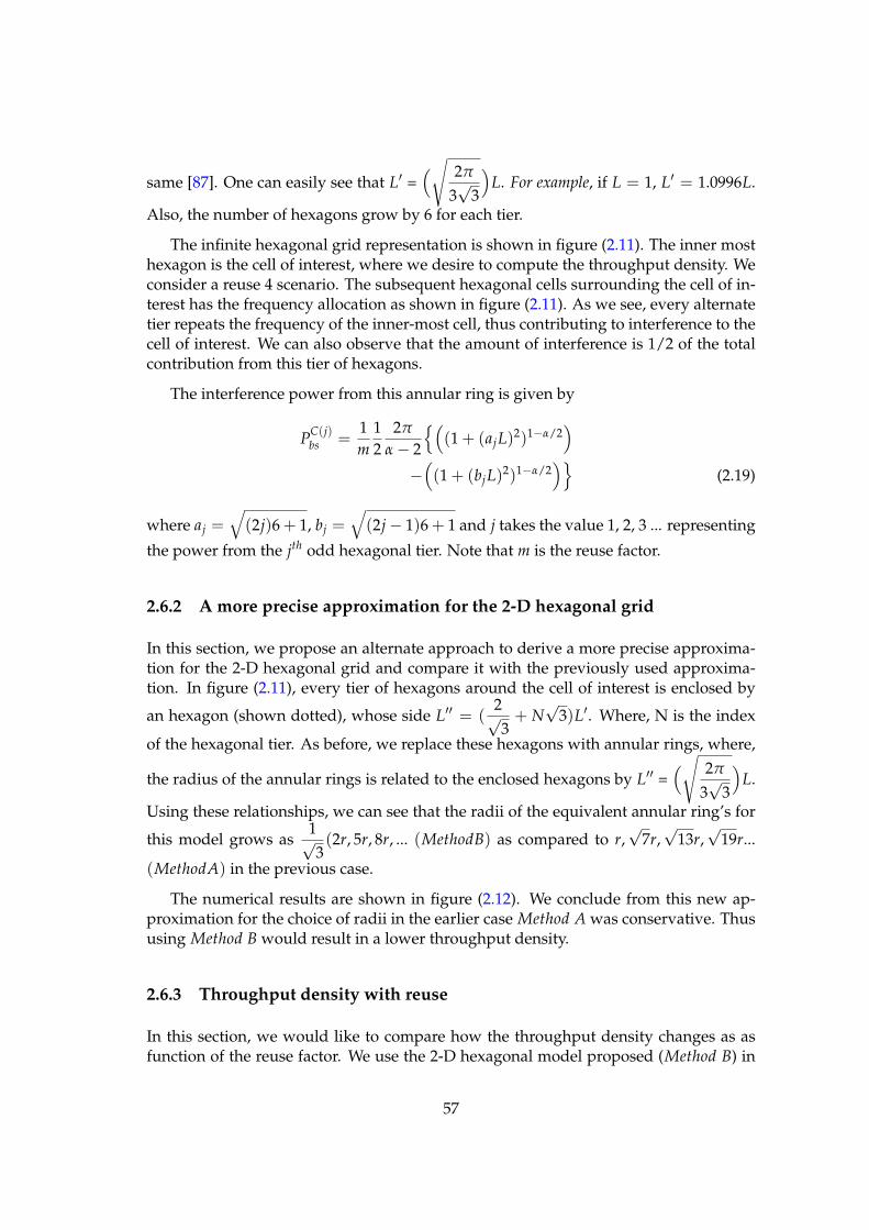
same [87]. One can easily see that L′ =(

√

2π

3√

3

)

L. For example, if L = 1, L′ = 1.0996L.

Also, the number of hexagons grow by 6 for each tier.

The infinite hexagonal grid representation is shown in figure (2.11). The inner mosthexagon is the cell of interest, where we desire to compute the throughput density. Weconsider a reuse 4 scenario. The subsequent hexagonal cells surrounding the cell of in-terest has the frequency allocation as shown in figure (2.11). As we see, every alternatetier repeats the frequency of the inner-most cell, thus contributing to interference to thecell of interest. We can also observe that the amount of interference is 1/2 of the totalcontribution from this tier of hexagons.

The interference power from this annular ring is given by

PC(j)bs =

1m

12

2π

α − 2

(

(1 + (ajL)2)1−α/2

)

−(

(1 + (bjL)2)1−α/2

)

(2.19)

where aj =√

(2j)6 + 1, bj =√

(2j − 1)6 + 1 and j takes the value 1, 2, 3 ... representing

the power from the jth odd hexagonal tier. Note that m is the reuse factor.

2.6.2 A more precise approximation for the 2-D hexagonal grid

In this section, we propose an alternate approach to derive a more precise approxima-tion for the 2-D hexagonal grid and compare it with the previously used approxima-tion. In figure (2.11), every tier of hexagons around the cell of interest is enclosed by

an hexagon (shown dotted), whose side L′′ = (2√3+ N

√3)L′. Where, N is the index

of the hexagonal tier. As before, we replace these hexagons with annular rings, where,

the radius of the annular rings is related to the enclosed hexagons by L′′ =(

√

2π

3√

3

)

L.

Using these relationships, we can see that the radii of the equivalent annular ring’s for

this model grows as1√3(2r, 5r, 8r, ... (MethodB) as compared to r,

√7r,

√13r,

√19r...

(MethodA) in the previous case.

The numerical results are shown in figure (2.12). We conclude from this new ap-proximation for the choice of radii in the earlier case Method A was conservative. Thususing Method B would result in a lower throughput density.

2.6.3 Throughput density with reuse

In this section, we would like to compare how the throughput density changes as asfunction of the reuse factor. We use the 2-D hexagonal model proposed (Method B) in

57

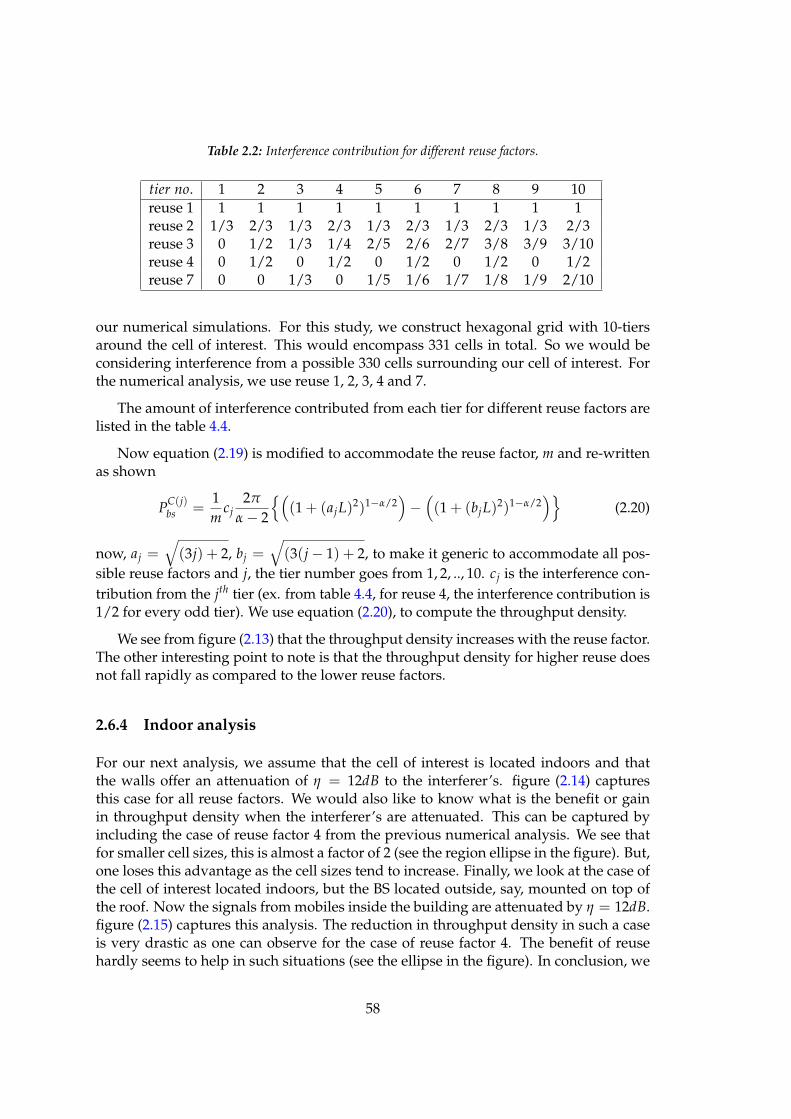
Table 2.2: Interference contribution for different reuse factors.

tier no. 1 2 3 4 5 6 7 8 9 10reuse 1 1 1 1 1 1 1 1 1 1 1reuse 2 1/3 2/3 1/3 2/3 1/3 2/3 1/3 2/3 1/3 2/3reuse 3 0 1/2 1/3 1/4 2/5 2/6 2/7 3/8 3/9 3/10reuse 4 0 1/2 0 1/2 0 1/2 0 1/2 0 1/2reuse 7 0 0 1/3 0 1/5 1/6 1/7 1/8 1/9 2/10

our numerical simulations. For this study, we construct hexagonal grid with 10-tiersaround the cell of interest. This would encompass 331 cells in total. So we would beconsidering interference from a possible 330 cells surrounding our cell of interest. Forthe numerical analysis, we use reuse 1, 2, 3, 4 and 7.

The amount of interference contributed from each tier for different reuse factors arelisted in the table 4.4.

Now equation (2.19) is modified to accommodate the reuse factor, m and re-writtenas shown

PC(j)bs =

1m

cj2π

α − 2

(

(1 + (ajL)2)1−α/2

)

−(

(1 + (bjL)2)1−α/2

)

(2.20)

now, aj =√

(3j) + 2, bj =√

(3(j − 1) + 2, to make it generic to accommodate all pos-sible reuse factors and j, the tier number goes from 1, 2, .., 10. cj is the interference con-tribution from the jth tier (ex. from table 4.4, for reuse 4, the interference contribution is1/2 for every odd tier). We use equation (2.20), to compute the throughput density.

We see from figure (2.13) that the throughput density increases with the reuse factor.The other interesting point to note is that the throughput density for higher reuse doesnot fall rapidly as compared to the lower reuse factors.

2.6.4 Indoor analysis

For our next analysis, we assume that the cell of interest is located indoors and thatthe walls offer an attenuation of η = 12dB to the interferer’s. figure (2.14) capturesthis case for all reuse factors. We would also like to know what is the benefit or gainin throughput density when the interferer’s are attenuated. This can be captured byincluding the case of reuse factor 4 from the previous numerical analysis. We see thatfor smaller cell sizes, this is almost a factor of 2 (see the region ellipse in the figure). But,one loses this advantage as the cell sizes tend to increase. Finally, we look at the case ofthe cell of interest located indoors, but the BS located outside, say, mounted on top ofthe roof. Now the signals from mobiles inside the building are attenuated by η = 12dB.figure (2.15) captures this analysis. The reduction in throughput density in such a caseis very drastic as one can observe for the case of reuse factor 4. The benefit of reusehardly seems to help in such situations (see the ellipse in the figure). In conclusion, we

58

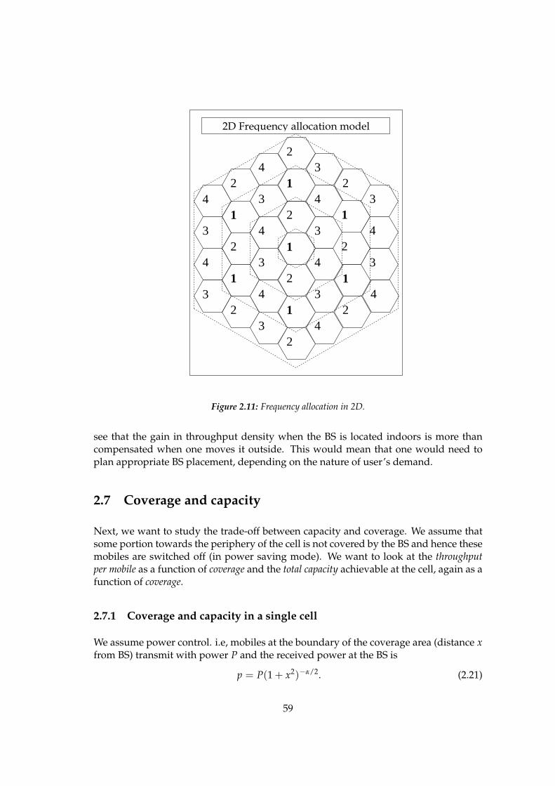
2

1

4

3

3

4

1

2

2

4

3

3

4

1

2

3

2

2

1

4

3

2

1

4

3

2

1

4

1

2

4

3

4

3

3

4

2

Figure 2.11: Frequency allocation in 2D.

see that the gain in throughput density when the BS is located indoors is more thancompensated when one moves it outside. This would mean that one would need toplan appropriate BS placement, depending on the nature of user’s demand.

2.7 Coverage and capacity

Next, we want to study the trade-off between capacity and coverage. We assume thatsome portion towards the periphery of the cell is not covered by the BS and hence thesemobiles are switched off (in power saving mode). We want to look at the throughputper mobile as a function of coverage and the total capacity achievable at the cell, again as afunction of coverage.

2.7.1 Coverage and capacity in a single cell

We assume power control. i.e, mobiles at the boundary of the coverage area (distance xfrom BS) transmit with power P and the received power at the BS is

p = P(1 + x2)−α/2. (2.21)

59

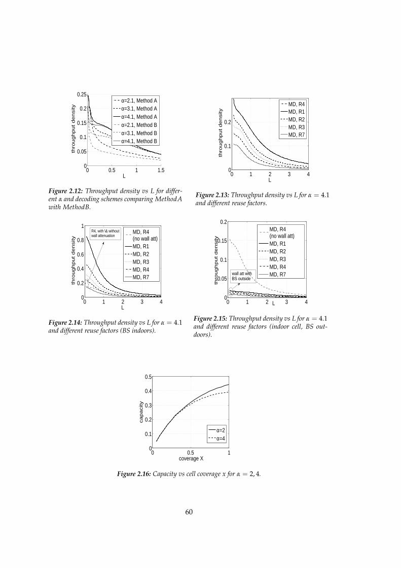
0 0.5 1 1.50

0.05

0.1

0.15

0.2

0.25

L

thro

ughput density

α=2.1, Method Aα=3.1, Method Aα=4.1, Method Aα=2.1, Method Bα=3.1, Method Bα=4.1, Method B

Figure 2.12: Throughput density vs L for differ-ent α and decoding schemes comparing MethodAwith MethodB.

0 1 2 3 40

0.1

0.2

L

thro

ughput density

MD, R4MD, R1MD, R2MD, R3MD, R7

Figure 2.13: Throughput density vs L for α = 4.1and different reuse factors.

0 1 2 3 40

0.2

0.4

0.6

0.8

1

L

thro

ughput density

MD, R4(no wall att)MD, R1MD, R2MD, R3MD, R4MD, R7

R4, with \& withoutwall attenuation

Figure 2.14: Throughput density vs L for α = 4.1and different reuse factors (BS indoors).

0 1 2 3 40

0.05

0.1

0.15

0.2

L

thro

ughput density

MD, R4(no wall att)MD, R1MD, R2MD, R3MD, R4MD, R7wall att with

BS outside

Figure 2.15: Throughput density vs L for α = 4.1and different reuse factors (indoor cell, BS out-doors).

0 0.5 10

0.1

0.2

0.3

0.4

0.5

coverage X

capacity

α=2α=4

Figure 2.16: Capacity vs cell coverage x for α = 2, 4.

60

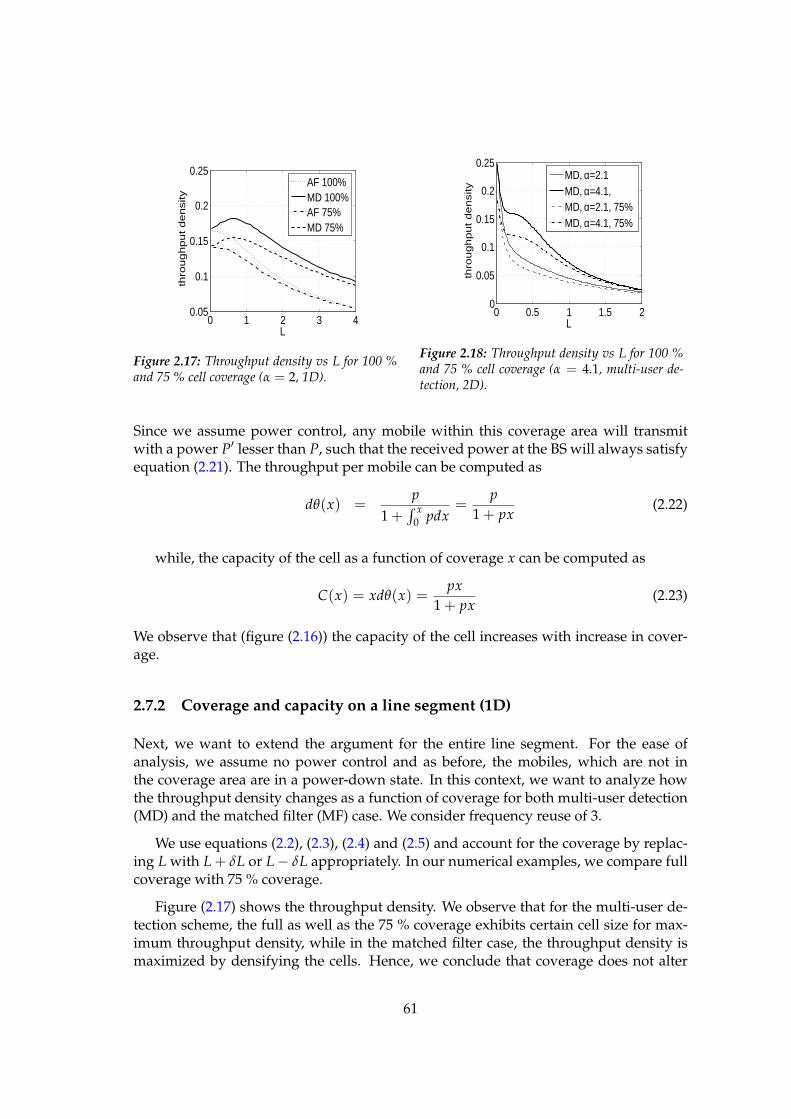
0 1 2 3 40.05

0.1

0.15

0.2

0.25

L

thro

ughput density

AF 100%MD 100%AF 75%MD 75%

Figure 2.17: Throughput density vs L for 100 %and 75 % cell coverage (α = 2, 1D).

0 0.5 1 1.5 20

0.05

0.1

0.15

0.2

0.25

L

thro

ughput density

MD, α=2.1MD, α=4.1,MD, α=2.1, 75%MD, α=4.1, 75%

Figure 2.18: Throughput density vs L for 100 %and 75 % cell coverage (α = 4.1, multi-user de-tection, 2D).

Since we assume power control, any mobile within this coverage area will transmitwith a power P′ lesser than P, such that the received power at the BS will always satisfyequation (2.21). The throughput per mobile can be computed as

dθ(x) =p

1 +∫ x

0 pdx=

p

1 + px(2.22)

while, the capacity of the cell as a function of coverage x can be computed as

C(x) = xdθ(x) =px

1 + px(2.23)

We observe that (figure (2.16)) the capacity of the cell increases with increase in cover-age.

2.7.2 Coverage and capacity on a line segment (1D)

Next, we want to extend the argument for the entire line segment. For the ease ofanalysis, we assume no power control and as before, the mobiles, which are not inthe coverage area are in a power-down state. In this context, we want to analyze howthe throughput density changes as a function of coverage for both multi-user detection(MD) and the matched filter (MF) case. We consider frequency reuse of 3.

We use equations (2.2), (2.3), (2.4) and (2.5) and account for the coverage by replac-ing L with L + δL or L − δL appropriately. In our numerical examples, we compare fullcoverage with 75 % coverage.

Figure (2.17) shows the throughput density. We observe that for the multi-user de-tection scheme, the full as well as the 75 % coverage exhibits certain cell size for max-imum throughput density, while in the matched filter case, the throughput density ismaximized by densifying the cells. Hence, we conclude that coverage does not alter

61

the behavior of achievable maximum throughput, albeit at a different cell size for themulti-user detection case.

We observe that for small cell sizes, the throughput density (refer to figure (2.17))is proportional to the coverage. But, as cell size increases, the throughput density fordifferent coverage tends to converge.

2.7.3 Coverage and capacity in two dimension

Next, we look at coverage and capacity in 2-dimension. As before, we have an infinitehexagonal grid and our analysis assumes interference coming from hexagonal ringssurrounding the cell of interest. Here again, we consider full and 75 % cell coverageand compute throughput density for different values of α

The following are note-worthy observations (see figure (2.18)).

1. The achievable throughput density falls very sharply in the vicinity of a small cellradii, irrespective of the coverage.

2. We achieve a maximum throughput density proportional to the coverage. i.efor example, the MD scheme with 75 % coverage achieves about 75 % of maximumthroughput density of the full coverage case at small cell radii. But, as the cell sizeincreases, the achieve throughput density with 75 % coverage starts moving closer tothe full coverage case.

2.8 Conclusions and future perspectives

We study aspects of cell dimensioning with static users under fluid limits. We char-acterize the throughput achievable at the BS as a function of the cell size. The aim ofthis study is to investigate if there exists a cell size which maximizes the achievablethroughput. We derived explicit expressions for power and throughput for both singlefrequency and frequency reuse with different receiver configurations and numericallyanalyze the impact of the cell size on throughput for various 1D, 2D models in bothindoor and outdoor scenarios. Our first cut analysis used free space path loss and wedid not consider the impact of shadowing, fading, etc. The analysis shows that thethroughput achievable is not always maximized by densifying the base-stations (BS),but rather depends on a case to case basis on factors like deployment (1D, 2D, indoor,outdoor), frequency reuse, etc. Our initial analysis did not incorporate radio fading,shadowing effects, mobility of users, etc. It would be interesting to study the behaviorof throughput achieved as a function of cell size with these effects. Further, we as-sumed continuum of users, which would enable us to use fluid limits and thus obtainsimple explicit expressions and an initial insight into cell design. A more realistic situ-ation is to assume users at discrete points or users distributed randomly according tosome distribution. Properties of such distributions can be used to analyze and obtain

62

dimensioning rules. It would be interesting to compare these results in the limitingregime.

2.9 Publications

1. Sreenath Ramanath, Eitan Altman, Vinod Kumar, Merouane Debbah, "Optimiz-ing cell size in pico-cell networks", proceedings of the Workshop on ResourceAllocation in Wireless Networks (RAWNET’09), Jun 27, Seoul, South Korea.

63

Chapter 3

Spatial Queueing Analysis forDesign and Dimensioning of SmallCell Networks with Mobile Users


3.2 System Model . . . . . . . . . . . . . . . . . . . . . . . . . . . . . . . . . 68

3.3 System Analysis . . . . . . . . . . . . . . . . . . . . . . . . . . . . . . . 69

3.4 Mobility on a street grid . . . . . . . . . . . . . . . . . . . . . . . . . . . 78

3.5 Mobility Examples . . . . . . . . . . . . . . . . . . . . . . . . . . . . . . 79

3.6 Call drops at Small cell boundaries (NES calls) . . . . . . . . . . . . . 80

3.7 Conclusions and Future work . . . . . . . . . . . . . . . . . . . . . . . 85

3.8 Appendix M: Calculations related to Macro queue . . . . . . . . . . . 86

3.9 Appendix P: Calculations for Small cell queue . . . . . . . . . . . . . 88

3.10 Publications . . . . . . . . . . . . . . . . . . . . . . . . . . . . . . . . . . 90

3.1 Introduction

In this chapter, we study cell design and dimensioning with mobile users.

To prevent a large number of handovers that would result from the small size of thecells ([127, 4]), it has been proposed to group together a number of Small cells in onevirtual Macrocell and to restrict the effort of preventing losses due to the handover onlyto those handovers that occur between Small cells of the same virtual cell. In betweenthe Small cells some fast switching mechanisms are proposed such as frequency follow-ing mechanism where the frequency used by a mobile follows it from one Small cell tothe next. This requires reserving the same channel for a user in the entire Macrocell.

65

In this chapter, we consider a large Macrocell divided into a number of Small cellsand study the impact of mobility on such systems, especially the effect of frequent han-dovers. We assume that the ongoing call is never dropped at the Small cell boundary,however base station switching (BSS) at any Small cell boundary requires some fixedamount of information (in terms of bytes) to be exchanged. There is however a possibil-ity of calls being dropped at Macrocell boundaries. We further assume that the activeusers cross Macrocell boundaries at maximum once, i.e., the calls always end beforereaching the second Macro boundary. The handovers at the Macrocell boundaries aremodeled as independent Poisson process (this is a commonly made assumption, forexample see [108, 53]).

We have several goals. First, to model the system so as to predict its performancemeasures. We are thus interested in developing tools using spatial queuing , that takeinto account not only the instantaneous geometry but also the way it varies in time. Itshould thus account for the impact of the speed of the users. We model the Macrocellsby various types of queues and well known results from queuing theory (for example[164]) are used to obtain performance measures like expected waiting time , expectedservice time , drop or blocking probabilities , etc. We shall use these results for prelimi-nary dimensioning purposes in planning the Small cell network catering to pedestrianand vehicular mobility, typical of urban and sub-urban areas. We derive closed formexpressions of useful performance metrics considering free space path loss, handoverconstraints, traffic type etc. We also obtain closed form expressions for optimal cell size,optimal for various performance metrics, when all the users move at the same fixed ve-locity. To derive these performance measures, we would require the moments of thetime taken by the system to serve1 the customers, which in our case will equivalentlybe the time the Macrocell spends on a call. We derive the expressions for these servicetimes, during which the information is exchanged between the moving user and theset of appropriate base stations (which it encounters during its journey), using variablerate of transmission. We further simplify the expressions for service time under thefollowing assumption: in a typical Small cell network, a moving user would have tra-versed across a number of cells before the completion of call. In this system, arrivalsoccur in space and the service time depend on the position, movement of the user andthe serving base station(s). The queues modeling these systems are referred to as spa-tial queues and have been used in interesting applications ([170, 88, 125, 18]). We makethe following theoretical and or simulation based observations:

1) Maximum possible velocity: For any fixed power of transmission P, there exists amaximum user velocity Vlim(P) and the users moving at speeds greater than Vlim cannot successfully communicate with the BS;

2) Larger cells for larger velocities: Given P, the optimal cell size increases with an in-crease in the highest velocity that the system has to support. This is true as long asthe highest velocity is less than Vlim(P). However the system cannot cater for velocitiesabove the limit Vlim(P), even if one increases the cell size indefinitely;

3) Insensitivity to application: The optimal cell size remains the same for non-elastic

1Throughout we use the terms from queuing theory like arrivals, service time etc.

66

(NES) as well as elastic (ES) calls for large file sizes, when the rest of the parametersremain same;

4) Two dimensional Manhattan Grid: The one dimensional results can be applied di-rectly to a two dimensional regular street grid (for example [103, 14]).

We extended the analysis to systems, where (negligible number of ) call drops canalso occur at Small cell boundaries, and obtained some initial results. To completelyavoid call drops at Small cell boundaries, one needs a centralized call admission con-trol (a control based on the total number of calls in the entire Macrocell). This require-ment can be relaxed if one can design a system delivering required QoS, in spite of(negligible) call drops at Small cell boundaries. We consider one such system (with de-centralized call admission control) and obtain closed form expressions for the optimalcell size catering to non elastic traffic.

In [118], we extended the analysis to a hexagonal 2D cellular structure in which theusers can move in any direction across the cell. The 2D system also considers possibledrops at Small cell boundaries as well as works with a more distributed call manage-ment system.

Several authors have examined the impact of mobility on the performance of wire-less networks. The authors in [72], have shown that mobility in fact increases the ca-pacity in ad hoc networks. In [21], the authors discuss the trade off between delay andachievable throughput in the presence of mobility in wireless ad-hoc networks. Fur-ther, In [28, 29, 36, 35], the authors discuss the impact of inter and intra-cell mobility oncapacity, flow level performance, trade-off between throughput and fairness, etc. Theyshow that mobility tends to increase the capacity with globally optimal as well as fairsharing policies, when the base stations interact. In conclusion, we see that the mobility(via multiuser diversity, opportunistic scheduling etc) can in fact improve the overallperformance of the system. However, most of the work assume that the handoversoccurs without extra cost. But in reality, each handover requires exchange of some in-formation between the user and the new BS and has a risk of not finding free resourcesin the new cell. Our work mainly focuses on these issues which become significantwhenever the frequency of handovers increases, as in the case of Small cell networks.

We describe our system in Section 3.2 while the service time is discussed in Sub-section 3.3.1 and is optimized in 3.3.6. The NES, ES calls are modeled by appropriatequeuing models and performance measures are derived in Subsections 3.3.8, 3.3.9 re-spectively. The two dimensional regular street grid is studied in Section 3.4 while thenumerical examples are provided in Section 3.5. Some initial results on a system withpossible call drops at Small cell boundaries and with a decentralized call admissioncontrol are in Section 3.6. Some lengthy derivations are provided in two appendices(Appendix M and P) placed at the end of the chapter.

67

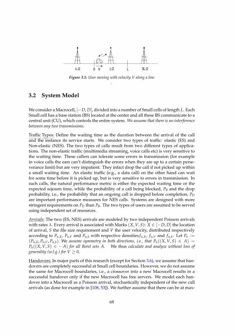
Figure 3.1: User moving with velocity V along a line

.

3.2 System Model

We consider a Macrocell, [−D, D], divided into a number of Small cells of length L. EachSmall cell has a base station (BS) located at the center and all these BS communicate to acentral unit (CU), which controls the entire system. We assume that there is no interferencebetween any two transmissions.

Traffic Types: Define the waiting time as the duration between the arrival of the calland the instance its service starts. We consider two types of traffic: elastic (ES) andNon-elastic (NES). The two types of calls result from two different types of applica-tions. The non-elastic traffic (multimedia streaming, voice calls etc) is very sensitive tothe waiting time. These callers can tolerate some errors in transmission (for examplein voice calls the ears can’t distinguish the errors when they are up to a certain perse-verance limit) but are very impatient. They infact drop the call if not picked up withina small waiting time. An elastic traffic (e.g., a data call) on the other hand can waitfor some time before it is picked up, but is very sensitive to errors in transmission. Insuch calls, the natural performance metric is either the expected waiting time or theexpected sojourn time, while the probability of a call being blocked, PB and the dropprobability, i.e., the probability that an ongoing call is dropped before completion, PD

are important performance measures for NES calls. Systems are designed with morestringent requirements on PD than PB. The two types of users are assumed to be servedusing independent set of resources.

Arrivals: The two (ES, NES) arrivals are modeled by two independent Poisson arrivalswith rates λ. Every arrival is associated with Marks (X, V, S): X ∈ [−D, D] the locationof arrival, S the file size requirement and V the user velocity, distributed respectivelyaccording to Pn,X, Pn,V and Pn,S with respective densities fn,X, fn,V and fn,S. Let Pn :=(Pn,X, Pn,V , Pn,S). We assume symmetry in both directions, i.e., that Pn((X, V, S) ∈ A) =Pn((X, V, S) ∈ −A) for all Borel sets A. We thus calculate and analyze without loss ofgenerality (w.l.g.) for V ≥ 0.

Handovers: In major parts of this research (except for Section 3.6), we assume that han-dovers are completely successful at Small cell boundaries. However, we do not assumethe same for Macrocell boundaries, i.e., a crossover into a new Macrocell results in asuccessful handover only if the new Macrocell has free servers. We model each han-dover into a Macrocell as a Poisson arrival, stochastically independent of the new callarrivals (as done for example in [108, 53]). We further assume that there can be at max-

68

imum one handover, i.e., the calls get finished before reaching the second Macrocellboundary. This simplifies the analysis to a good extent and is quite a good assumptionas the Macrocells are typically large in dimension. We consider generalization of thisassumption in our future work. Lastly in Section 3.6 we obtain some initial results byrelaxing the ’handovers at Small cell boundaries are completely successful’ assumption.

Radio Conditions: The BS communicates with the mobiles using a wireless link, at a ratethat depends upon the distance between the two. Since our primary focus is on mobil-ity we implicitly consider Small cells deployed outdoors, for example urban, suburbanscenarios. Hence we can assume significant line of sight signal. Further, Small cells be-ing small in size, it will be sufficient to consider only the direct path for communication.A user located at x communicates with BS of cell m using unit transmit power (whenreceiver noise variance is one) at rate2 given by,

R(x; m) := 1|x−(mL− L2 )|≤d0 + 1|x−(mL− L

2 )|>d0d0β

∣

∣

∣

∣

x −(

mL − L

2

)∣

∣

∣

∣

−β

, (3.1)

where β ≥ 1 represents path loss factor and d0 > 0 is a small distance up to which thereis no propagation loss. The above model is valid for systems with low signal to noiseratios, where in the rates are directly given by the SNRs.

3.3 System Analysis

The users are moving continuously with a fixed but random velocity. The Macrocellcan handle at maximum K parallel calls. Transmission always occurs at fixed powerP. Since Small cells are small in size, the movement of the users results in frequenthandovers. The number of handovers will be quite large that it would be complicatedto design a reliable system without redundancy: We assume that every BS can alsohandle K parallel calls3. This ensures that, once a call is picked up it is not dropped atany Small cell boundary: when a user crosses over to a new BS, the new BS would atmaximum be handling K − 1 calls and hence will have at least one free server. Howeverit is important to note that the maximum power used at any time in the system equalsKP. We further assume that :

1) Every BSS (base station switching at a Small cell boundary) requires fixed Bh bytesof information to be communicated (independent of the user’s velocity), after which the

2The analysis will go through for any other rate functions, for example like R(x; 1) =

(1 + (x − L/2)2)−β/2 ([115]), R(x; 1) = log[

1 + (1 + (x − L/2)2)−β/2]

([115]), R(x; 1) =

log[

1 +(

dβ0 |x − L/2|−β 1|x−L/2|>d0 + 1|x−L/2|≤d0

)]

etc. Some of the simplifications that weobtain in subsequent sections, may not be possible with these rate functions. However one can alwaysconduct Monte Carlo simulations to obtain the required inferences.

3In practical systems, each BS will have M backup servers to manage handovers. This means eachBS can handle M parallel calls. In general M need not be equal to K, however M has to be chosen largeenough to ensure negligible call drops at Small cell boundaries, taking into consideration the large numberof handover associated with Small cells. With this large enough M the system’s behavior will be close tothe system considered in this work (the case with M = K).

69

user’s service is resumed by the BS of the cell it just entered;

2) The user is served by the BS of the Small cell in which it is moving, as it is physi-cally nearest to this BS.

In the following sections up to and excluding Section 3.6, all the results are derivedunder the assumption that, no call drops ever happen at Small cell boundaries.

3.3.1 Time required for communicating S bytes (Bc)

Define by Bc(S, X, V) the time required to communicate a packet of length S bytes toa user located at X (when the service starts) and moving with velocity V. If the usercan communicate at a fixed rate r bytes/sec then the communication time would havebeen S/r. The maximum rate at which a user can communicate with the BS in cell m isgiven by (3.1). This position dependent rate varies: minimum when the user is at thecell edges and increases as the user moves towards the cell center. This poses a needto calculate the communication time considering the variable rates. The location of theuser (under service) will change according to X(t) = X + Vt (Figure 3.1). At time t, if

the user is in cell m, i.e. if X(t) ∈ [(m − 1)L, mL], it communicates with the BS of mth

cell. Hence the user gets service at time varying rate given by

R(t; X, V) := PR(X(t); m) if t ∈[

(m − 1)L − X

V,

mL − X

V

]

.

Without loss of generality we consider the users, whose communication started in thefirst Small cell, i.e., with X ∈ [0, L]. The communication time Bc required by the user,i.e., the time required to communicate S bytes satisfies :

S =∫ Bc

0R(t; X, V)dt. (3.2)

Let, g(l) :=∫ l/V

0PR(Vt; 1)dt = P

∫ l

0R(l′; 1)

dl′

V,

represent the number of bytes communicated while the mobile traverses interval [0, l].Note that (throughout it is assumed that L > 2d0: one can easily show that the optimalcell size has to be greater than 2d0),

g(L) =Pd

β0

V

∫ L/2−d0

0

(

L

2− l

)−β

dl +Pd

β0

V

∫ L

L/2+d0

(

l − L

2

)−β

dl +2Pd0

V

=

2Pd0

V(β − 1)

(

β −(

L

2d0

)1−β)

when β > 1

2Pd0

V(log(L/2)− log(d0)) when β = 1.

(3.3)

For any m, the number of bytes communicated as the user traverses through mth Smallcell (by change of variable l = X + Vt − (m − 1)L),

∫ mL−XV

(m−1)L−XV

R(t; X, V)dt =∫ mL−X

V

(m−1)L−XV

PR(X + Vt; m)dt =P

V

∫ L

0R(l; 1)dl = g(L)

70

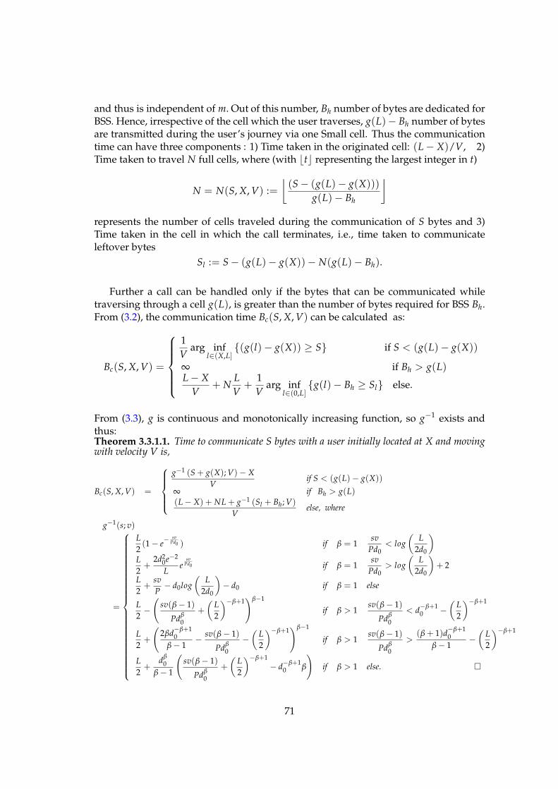
and thus is independent of m. Out of this number, Bh number of bytes are dedicated forBSS. Hence, irrespective of the cell which the user traverses, g(L)− Bh number of bytesare transmitted during the user’s journey via one Small cell. Thus the communicationtime can have three components : 1) Time taken in the originated cell: (L − X)/V, 2)Time taken to travel N full cells, where (with ⌊t⌋ representing the largest integer in t)

N = N(S, X, V) :=⌊

(S − (g(L)− g(X)))

g(L)− Bh

⌋

represents the number of cells traveled during the communication of S bytes and 3)Time taken in the cell in which the call terminates, i.e., time taken to communicateleftover bytes

Sl := S − (g(L)− g(X))− N(g(L)− Bh).

Further a call can be handled only if the bytes that can be communicated whiletraversing through a cell g(L), is greater than the number of bytes required for BSS Bh.From (3.2), the communication time Bc(S, X, V) can be calculated as:

Bc(S, X, V) =

1V

arg infl∈(X,L]

(g(l)− g(X)) ≥ S if S < (g(L)− g(X))

∞ if Bh > g(L)L − X

V+ N

L

V+

1V

arg infl∈(0,L]

g(l)− Bh ≥ Sl else.

From (3.3), g is continuous and monotonically increasing function, so g−1 exists andthus:Theorem 3.3.1.1. Time to communicate S bytes with a user initially located at X and movingwith velocity V is,

Bc(S, X, V) =

g−1 (S + g(X); V)− X

Vif S < (g(L)− g(X))

∞ if Bh > g(L)(L − X) + NL + g−1 (Sl + Bh; V)

Velse, where

g−1(s; v)

=

L

2(1 − e

− svPd0 ) if β = 1

sv

Pd0< log

(

L

2d0

)

L

2+

2d20e−2

Le

svPd0 if β = 1

sv

Pd0> log

(

L

2d0

)

+ 2

L

2+

sv

P− d0log

(

L

2d0

)

− d0 if β = 1 else

L

2−(

sv(β − 1)

Pdβ0

+

(

L

2

)−β+1)β−1

if β > 1sv(β − 1)

Pdβ0

< d−β+10 −

(

L

2

)−β+1

L

2+

(

2βd−β+10

β − 1− sv(β − 1)

Pdβ0

−(

L

2

)−β+1)β−1

if β > 1sv(β − 1)

Pdβ0

>(β + 1)d−β+1

0β − 1

−(

L

2

)−β+1

L

2+

dβ0

β − 1

(

sv(β − 1)

Pdβ0

+

(

L

2

)−β+1− d

−β+10 β

)

if β > 1 else.

71

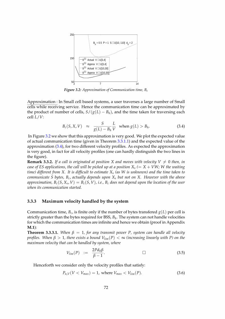
2 7 1450

150

250

b(1) Actual V ∼ U[3,4]

b(1) Approx V ∼ U[3,4]

b(1) Actual V ∼ U[10,30]

b(1) Approx V ∼ U[10,30]

Bh = 0.5 P = 1 S ∼ U[10, 110] d

0 = 2

Figure 3.2: Approximation of Communication time, Bc

Approximation : In Small cell based systems, a user traverses a large number of Smallcells while receiving service. Hence the communication time can be approximated bythe product of number of cells, S/(g(L)− Bh), and the time taken for traversing eachcell L/V:

Bc(S, X, V) ≈ S

g(L)− Bh

L

Vwhen g(L) > Bh. (3.4)

In Figure 3.2 we show that this approximation is very good. We plot the expected valueof actual communication time (given in Theorem 3.3.1.1) and the expected value of theapproximation (3.4), for two different velocity profiles. As expected the approximationis very good, in fact for all velocity profiles (one can hardly distinguish the two lines inthe figure).Remark 3.3.2. If a call is originated at position X and moves with velocity V 6= 0 then, incase of ES applications, the call will be picked up at a position Xs (= X + VW; W the waitingtime) different from X. It is difficult to estimate Xs (as W is unknown) and the time taken tocommunicate S bytes, Bc, actually depends upon Xs but not on X. However with the aboveapproximation, Bc(S, Xs, V) = Bc(S, V), i.e., Bc does not depend upon the location of the userwhen its communication started.

3.3.3 Maximum velocity handled by the system

Communication time, Bc, is finite only if the number of bytes transfered g(L) per cell isstrictly greater than the bytes required for BSS, Bh. The system can not handle velocitiesfor which the communication times are infinite and hence we obtain (proof in AppendixM.1):Theorem 3.3.3.1. When β = 1, for any transmit power P, system can handle all velocityprofiles. When β > 1, there exists a bound Vlim(P) < ∞ (increasing linearly with P) on themaximum velocity that can be handled by system, where

Vlim(P) :=2Pd0β

β − 1. (3.5)

Henceforth we consider only the velocity profiles that satisfy:

Pn,V(V < Vmax) = 1, where Vmax < Vlim(P). (3.6)

72

3.3.4 Service time : The time of the Macrocell spent for user’s service

The user reaches the boundary of the Macrocell starting from a point X in time:

B∂(X, V) :=D − X

V. (3.7)

The Macrocell has to serve the user either until all its S bytes are transmitted (whichtakes time Bc) or till the user reaches the boundary. Thus, the overall service time re-quirement of the user in a Macrocell is BD := min(D − Xs)/V, Bc(V, S), where Xs

(defined in Remark 3.3.2) is the user position when its service starts. By Remark 3.3.2,Bc does not depend upon Xs. For NES applications Xs = X the position of arrival. ForES applications, it is difficult to estimate Xs, instead we approximate Xs with X, i.e.,BD(X, V, S) ≈ minB∂(X, V), Bc(V, S). The error in this approximation is given (withW representing the waiting time) by:

Err = W1Bc>D−X

V +

(

Bc −D − Xs

V

)

1 D−XsV <Bc<

D−XV

and so for any k,

E[Ekrr] ≤ E

[

Wk1Bc>D−X

V −W]

.

The error is small either whenever the number of servers is large (so waiting times are small) orwhen the Macrocell is large in size (which usually is the case).

3.3.5 Macro Handovers

Handover are modeled as Poisson arrivals (as done in [108, 53]). In this subsection wederive the other characteristics of the handover calls.

Distribution of handover call marks (X, S): In general handover densities will be differ-ent from the new call densities fn,X, fn,S and fn,V . As the users move in either directionwith equal probability, Ph,X the position of handover arrival occurs either at −D orat D with half probability. If handover occurs at −D the corresponding velocity willbe positive, which is the case we consider w.l.g. We assume fn,S is exponential, i.e.,fn,S(s) = µe−µs for some µ > 0, in which case by memoryless property, fh,S = fn,S.

Rate of handovers: Let

ν(v, L) :=η(L)− vBh

L= v

g(L)− Bh

L. (3.8)

Then from (3.4) and (3.7),

Pho := Prob(B∂ < Bc) = En,X,V

[

e−µν(V,L)(D−X)/V]

(3.9)

gives the probability that a call is not completed in one Macrocell. This precisely repre-sents that fraction of new arrivals which get converted into handover calls. So

λho := λPho

73

is the rate at which handovers occur.

Speed of handover arrival : A handover call arrives at X = −D with velocity v > 0only if a new call with velocity v is not completed before reaching the boundary. Herewe use the assumption that handover occurs at maximum at one Macrocell boundary,i.e., an handover call is not converted to another handover. Let

Pho,v := Prob(B∂ < Bc|v) = En,X

[

e−µν(v,L)(D−X)/v]

(3.10)

represent the conditional probability given V = v. Then the handover speed distribu-tion,

fh,V(v) =fn,V(v)Pho,v

Pho.

3.3.6 Moments of Service time

Under assumption (3.6), the kth moment of BD exists (whenever the correspondingfor S and V−1 exist) and equals, b(k) := EX,V,S[(BD(X, V, S))k], where EX,V,S is theexpectation w.r.t. the (new call and handover call) joint distribution,

PX,V,S :=λ(Pn,X, Pn,V , Pn,S) + λho(Ph,X,V , Ph,S)

λ + λho.

In Appendix M.2 we obtain (recall En is expectation w.r.t. Pn, the new call distribution):

b(k) = En

[

BD(x, v, s)k + BD(−D, v, s)kPho,v

1 + Pho

]

and (3.11)

db(k)

dL= En

[

d

dL

(


1 + Pho

)]

. (3.12)

3.3.7 Cell size optimizing the moments of the service time

The number of bytes that can be communicated in a cell increases with the increasein cell size: from (3.3) g is continuous and monotonically increasing w.r.t. L. For anygiven velocity there exists a minimum cell size (the smallest cell size at which one cantransmit more than Bh bytes per cell), below which successful communication is notpossible. When cell size is closer to this smallest one, the useful bytes transmitted percell (g(L) − Bh) are very small and hence it takes more time to transmit S bytes, i.e.,the communication time Bc will be large. As the cell size increases from this smallestsize, the communication time Bc starts reducing. However after some point, due topath loss, the number of bytes per cell starts saturating and hence the gain in termsof useful bytes transmitted per cell will be small in comparison with the extra timetaken to traverse each cell, resulting in increasing the communication time again. Thus

74

there exists an optimal cell size for every fixed velocity. One can extrapolate similar thingseven for random velocity. We derive the optimal cell size L∗

b(1)and relate the same to

the optimizer of more interesting performance measures for ES and NES calls in thesubsequent sub-sections.

Define L∗ν(v) := arg max

Lν(v, L), the maximizer of the function ν given by (3.8). In

Appendix M.3 we show that, there exists an unique L∗ν(v) > 0 for every velocity v.

In the Appendix M.4 we further show that, for fixed velocities (i.e., when V ≡ v), the

derivatives of all the (existing) kth moments of the service time vanish only at L∗ν(v).

Thus for fixed velocities, all the (existing) moments of the service time have unique and commonminima:

L∗b(k)

:= arg minL

b(k) = arg maxL

ν(v, L) = L∗ν(v) for all k.

The common optimizer L∗ (for example for β > 1) satisfies

∂ν(v, L)

∂L

∣

∣

∣

∣

L=L∗= 0 or 2P

(

L∗

d0

)−β

L∗ − η(L∗) + vBh = 0 and therefore

Theorem 3.3.7.1. For fixed velocity profile, i.e., Pn,V(V = v) = 1 the optimal cell size for theexpected service time is,

L∗b(1)

= L∗ν =

2

2Pdβ0

ββ−1

2Pd0β

β−1 − vBh

1β−1

when β > 1

2d0evBh

2Pd0 when β = 1.

Further, if the kth moment of the service time exists then L∗b(k)

= L∗b(1)

.

For velocity profiles with small variance, the optimizers of all the moments of the servicetime will be equal approximately. Hence when Pn,V has small variance with mean v thenL∗

b(1)is close to L∗

ν(v) . From the above it is clear that L∗b(1)

increases when the mean v increases.

Having obtained the service time, we now turn our attention to model variousconfigurations of the Macrocell with appropriate queues to further obtain their per-formance measures.

3.3.8 ES Calls : Average Waiting time

Each Macrocell can handle at maximum K parallel calls. The CU of the Macrocell keepsa record of the users entered into the system and serves them in FIFO (first in first out)order via the BSs of the Small cells. When a new user initiates a call, it is immediatelypicked up if there are less than K active calls in the system. If not the user will haveto wait. Its service will start at the time : 1) when one of the active K users finish theirservice and exit 2) if there are no other waiting users arrived before it. The BS nearest tothe user, at the time of its service start, will initiate the call. Hence after, its call is served(by the Macrocell under consideration) as discussed in subsection 3.3.1 either till its

75

service is over or till it reaches the Macrocell boundary. When it reaches the boundarythe call will be transfered to the next Macrocell as a handover call and the handovercall is treated by the new cell similar to that of a new call. Thus each Macrocell can bemodeled by a M/G/K queue with service time BD and Poisson arrivals at rate λ + λho.This queue has been analyzed to a good extent and the system is stable only if ([140])

ρ :=(λ + λho)b

(1)

K< 1.

For stable queues, the expected waiting time of a randomly arrived customer can beapproximated by ([140]):

E[W]K =

(

b(2)

2(b(1))2

)(

b(1)

K(1 − ρ)

)

(

(Kρ)K

K!

)

π0; π−10 =

(Kρ)K

K!+ (1 − ρ)

K−1

∑i=0

(Kρ)i

i!.(3.13)

where b(1), b(2) are given by (3.11). If the system is unstable the number of waitingcustomers grows towards infinity and thus one should consider only the cell sizes Lwith ρ < 1. Hence, the optimal size, which minimizes (3.13) is

L∗ES := arg min

L:ρ<1E[W]K.

We saw in the previous section that the optimizer of b(2) is same as that of b(1) for fixedvelocities and will be close to each other for smaller velocity variances. In a similar waythe same thing is true for ρ, i.e., for fixed velocities,

L∗ρ := arg min

L:ρ<1ρ = L∗

b(1).

The expected waiting time (3.13) is continuously differentiable in b(1), b(2) and ρ. Thus(minimizer of (3.13) is a zero of its derivative and E[W]K depends upon L only via b(1),b(2), ρ),Theorem 3.3.8.1. Optimal cell size for a system with elastic traffic, with Pn,V(V = v) = 1 is,

L∗ES = arg min

L:ρ<1E[W]k = L∗

b(1).

So, L∗b(1)

minimizes both expected waiting time and expected service time. Also, it minimizesthe expected sojourn time, as it is the sum of expected waiting and service times.

Also from (3.13), when L∗b(1)

and L∗b(2)

are close, it is easy to see that the optimizer ofE[W]K will be close to that of the expected service time, b(1). Thus even for low velocityvariances,

L∗ES ≈ arg min

L:ρ<1b(1) = L∗

b(1).

We see that this is true even for many general velocity profiles in examples section 3.5.

76

3.3.9 NES Calls : Block and Drop Probabilities

As before the system can handle at maximum K parallel calls. The call is picked upimmediately (by the BS of the Small cell in which the call is originated) only if theMacrocell is serving lesser than K users at the time of its arrival. If all the K servers arebusy it is dropped. When an active customer reaches the boundary of a Macrocell, itscall is continued in the next Macrocell only if the new Macrocell has free servers. EachMacrocell can thus be modeled by an M/G/K/K queue. And its call block probabilityis given by the Erlang Loss formula (ρ was defined in previous section),

PB(L) =ρ(L)K/K!

∑Kk=0 ρ(L)k/k!

.

It is interesting to note that PB(L) and ρ are both differentiable w.r.t. L and further thatif the derivative dρ/dL is zero at a L∗ so is the derivative dPB/dL. By taking the secondderivative, we can in fact show that their minimizers are the same. Hence,

L∗PB

= arg minL:ρ(L)<1

PB(L) = L∗ρ.

Further at fixed velocities, L∗ρ = L∗

b(1)and so we have,

Theorem 3.3.9.1. The minimizer, L∗b(1)

also minimizes the block probability, PB, for fixed veloc-ities. For any velocity profile, L∗

ρ also minimizes the block probability.

Drop Probability : Under the assumptions stated earlier, only a new call can reachthe boundary and not a call which was already handed over once. Further, an activecall is dropped only when it reaches the Macrocell boundary and the new Macrocell isbusy. By independence of the two events (status of the new Macrocell prior to handoveris independent of the call that is handed over), the drop probability is

PD(L) = PhoPB(L).

One can design an optimal system, catering to NES calls, either by jointly mini-mizing both the block and drop probabilities or by minimizing one of the probabilitieswhile placing a constraint on the other. Usually systems are designed with more strin-gent requirements on PD than on PB. We note from the above calculations that PD isdirectly proportional to PB and will be smaller than PB by a factor Pho. We make inthe rest of this subsection, a commonly made assumption that, the location of the callarrivals is uniformly distributed, i.e. that X ∼ U [−D, D]. Under this assumption:

Pho = Pn (B∂(X, V) < Bc(V, S)) = En,S,V [PX(D − X < VBc(V, S))]

=En,S,V

[

min

2D, VSLη(L)−VBh

]

2D

= En,V

[

e−µ2D(η(L)−VBh)/VL]

+E[

1 − e−µ2D(η(L)−VBh)/VL(

1 + 2Dµ(η(L)−VBh)VL

)]

2Dµ

< En,V

[

e−µ2D(η(L)−VBh)/VL]

+1

2Dµ.

77

Thus Pho decreases with 2D, the Macrocell size. Macrocells are large in dimension andhence PD can be ensured to be within the prescribed limits (the limit is a design param-eter) by directly minimizing PB itself. Thus we propose to choose cell size L to minimizePB and hence equivalently ρ:

L∗NES := L∗

ρ = arg minL:ρ(L)<1

ρ(L) ≈ L∗b(1)

.

Remark 3.3.10. Thus for both ES and NES applications one needs to minimize the first moment

of the service time, b(1), to obtain the optimal cell size. This optimal cell size has been discussedin the previous section for fixed velocities and for velocity profiles with small variances. Thegeneral situation is studied in section 3.5 via numerical examples.

3.4 Mobility on a street grid

We assume that users are moving in a rectangular grid overlaying a large area [−D, D]×[−D, D] with grid size b, d as shown in Figure 3.3. This example is typical of urban ar-eas where the streets are in a criss-cross manner (this is a well known model, see forexample [103, 14]) and hence is an interesting example for study.

In this case, we assume that the location of arrival X is uniformly distributed on thelines, i.e, X ∼ U [G], where the grid

G := ∪D/di=1 [−D, D]×

id +d

2

∪ ∪D/bi=1

ib +b

2

× [−D, D].

A one dimensional vector V represents the speed of the vehicle, which is uniformlydistributed, i.e., V ∼ U [0, Vmax] . It’s direction depends upon the position of arrivalX: it is horizontal if X is on horizontal line and is vertical if on vertical line. One caneasily extend the analysis to include zig-zag paths. In either case we assume it be equi-probable in the two possible directions; towards left or right in case of horizontal lineand towards up or down in case of vertical line.

Any Small cell is a line segment of a street and a base station is placed at the centerof this cell (if we neglect the small number of Small cells that might possibly span acrosstwo intersecting streets). The mobiles may change directions as they take a turn, butthe rate they obtain with their BS once again follows periodic pattern as explained insection 3.3.1. Hence the time to reach the boundary B∂, the time to serve S bytes BS andhence the service time BD are just the same as those derived in the previous sections.Thus the analysis and the results of all the previous sections is applicable to the grid structure.So in the grid structure, the 2 dimensional analysis actually boils down to one dimensionalanalysis itself.

78

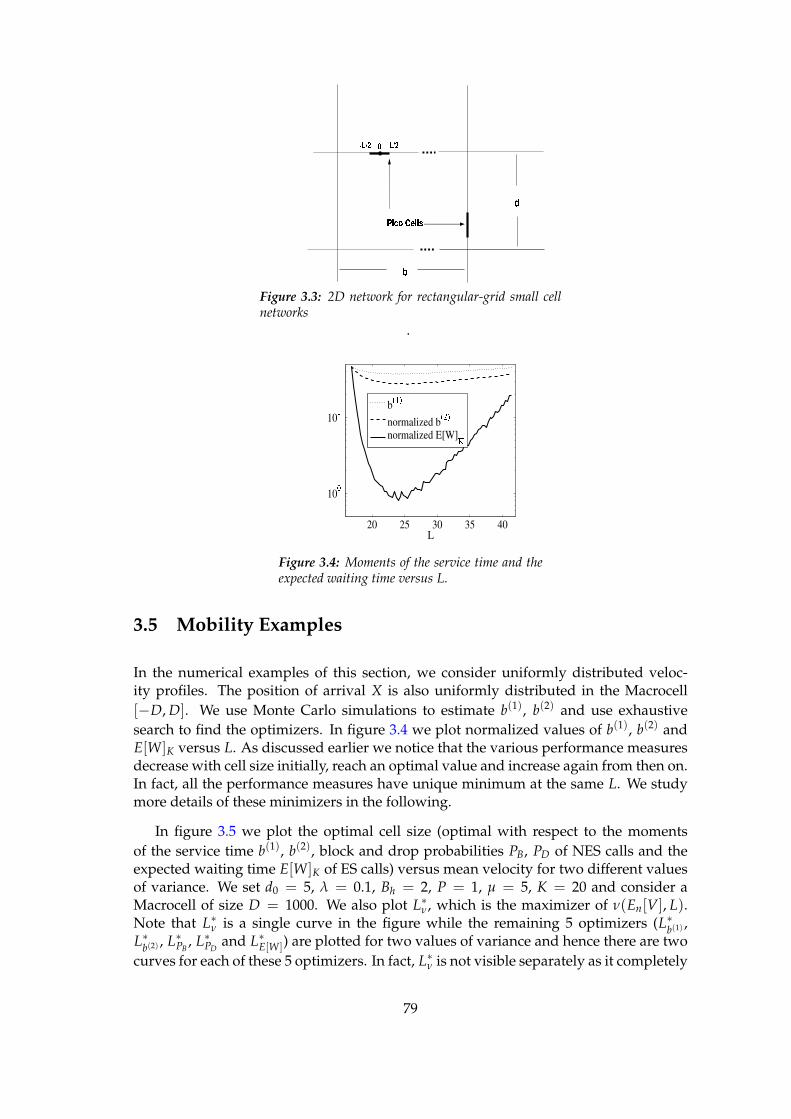
Figure 3.3: 2D network for rectangular-grid small cellnetworks

.

Figure 3.4: Moments of the service time and theexpected waiting time versus L.

3.5 Mobility Examples

In the numerical examples of this section, we consider uniformly distributed veloc-ity profiles. The position of arrival X is also uniformly distributed in the Macrocell[−D, D]. We use Monte Carlo simulations to estimate b(1), b(2) and use exhaustivesearch to find the optimizers. In figure 3.4 we plot normalized values of b(1), b(2) andE[W]K versus L. As discussed earlier we notice that the various performance measuresdecrease with cell size initially, reach an optimal value and increase again from then on.In fact, all the performance measures have unique minimum at the same L. We studymore details of these minimizers in the following.

In figure 3.5 we plot the optimal cell size (optimal with respect to the momentsof the service time b(1), b(2), block and drop probabilities PB, PD of NES calls and theexpected waiting time E[W]K of ES calls) versus mean velocity for two different valuesof variance. We set d0 = 5, λ = 0.1, Bh = 2, P = 1, µ = 5, K = 20 and consider aMacrocell of size D = 1000. We also plot L∗

ν, which is the maximizer of ν(En[V], L).Note that L∗

ν is a single curve in the figure while the remaining 5 optimizers (L∗b(1)

,L∗

b(2), L∗

PB, L∗

PDand L∗

E[W]) are plotted for two values of variance and hence there are twocurves for each of these 5 optimizers. In fact, L∗

ν is not visible separately as it completely

79

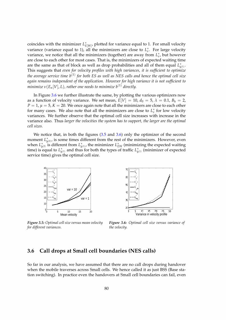
coincides with the minimizer L∗E[W], plotted for variance equal to 1. For small velocity

variance (variance equal to 1), all the minimizers are close to L∗ν. For large velocity

variance, we notice that all the minimizers (together) are away from L∗ν, but however

are close to each other for most cases. That is, the minimizers of expected waiting timeare the same as that of block as well as drop probabilities and all of them equal L∗

b(1).

This suggests that even for velocity profiles with high variances, it is sufficient to optimize

the average service time b(1) for both ES as well as NES calls and hence the optimal cell sizeagain remains independent of the application. However for high variance it is not sufficient to

minimize ν(En[V], L), rather one needs to minimize b(1) directly.

In Figure 3.6 we further illustrate the same, by plotting the various optimizers nowas a function of velocity variance. We set mean, E[V] = 10, d0 = 5, λ = 0.1, Bh = 2,P = 1, µ = 5, K = 20. We once again note that all the minimizers are close to each otherfor many cases. We also note that all the minimizers are close to L∗

ν for low velocityvariances. We further observe that the optimal cell size increases with increase in thevariance also. Thus larger the velocities the system has to support, the larger are the optimalcell sizes.

We notice that, in both the figures (3.5 and 3.6) only the optimizer of the secondmoment L∗

b(2), is some times different from the rest of the minimizers. However, even

when L∗b(2)

is different from L∗b(1)

, the minimizer L∗EW (minimizing the expected waiting

time) is equal to L∗b(1)

and thus for both the types of traffic L∗b(1)

(minimizer of expectedservice time) gives the optimal cell size.

0 5 10 15 205

10

15

20

25

30

35

40

Mean velocity

L*ν

L*b

(1)

L*b

(2)

L*EW

L*Pb

L*Pd var = 1

var = 10

Figure 3.5: Optimal cell size versus mean velocityfor different variances.

Figure 3.6: Optimal cell size versus variance ofthe velocity.

3.6 Call drops at Small cell boundaries (NES calls)

So far in our analysis, we have assumed that there are no call drops during handoverwhen the mobile traverses across Small cells. We hence called it as just BSS (Base sta-tion switching). In practice even the handovers at Small cell boundaries can fail, even

80

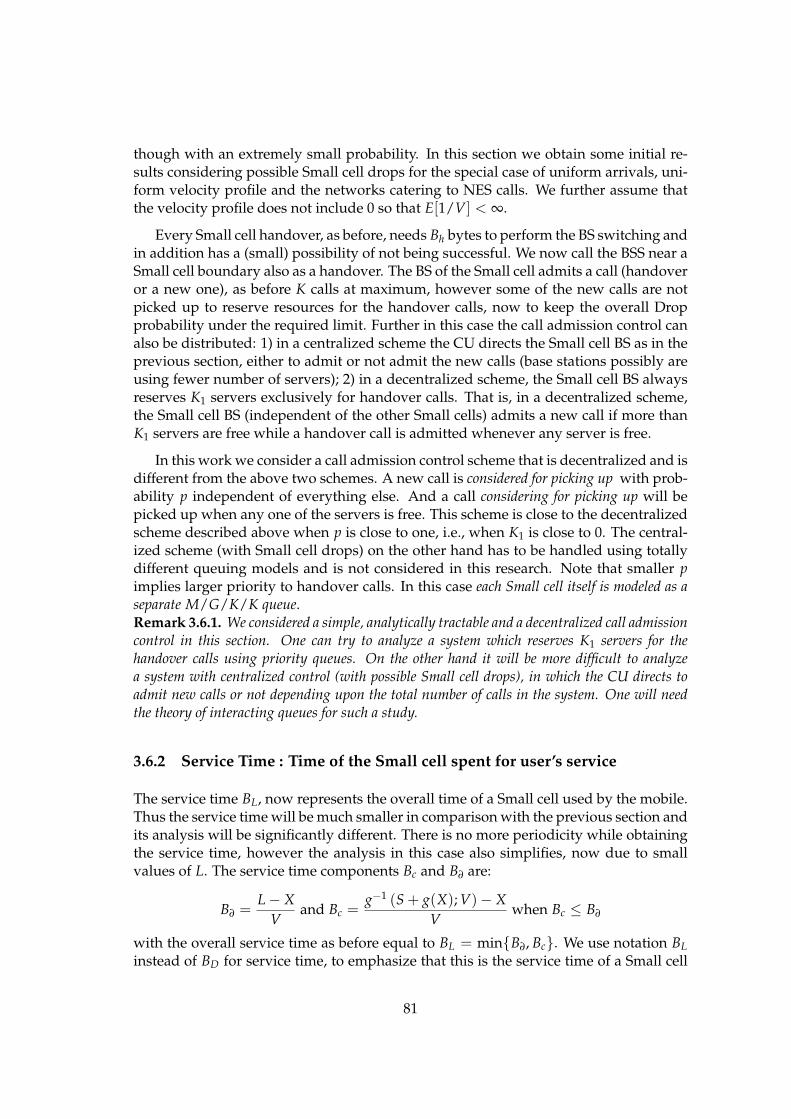
though with an extremely small probability. In this section we obtain some initial re-sults considering possible Small cell drops for the special case of uniform arrivals, uni-form velocity profile and the networks catering to NES calls. We further assume thatthe velocity profile does not include 0 so that E[1/V] < ∞.

Every Small cell handover, as before, needs Bh bytes to perform the BS switching andin addition has a (small) possibility of not being successful. We now call the BSS near aSmall cell boundary also as a handover. The BS of the Small cell admits a call (handoveror a new one), as before K calls at maximum, however some of the new calls are notpicked up to reserve resources for the handover calls, now to keep the overall Dropprobability under the required limit. Further in this case the call admission control canalso be distributed: 1) in a centralized scheme the CU directs the Small cell BS as in theprevious section, either to admit or not admit the new calls (base stations possibly areusing fewer number of servers); 2) in a decentralized scheme, the Small cell BS alwaysreserves K1 servers exclusively for handover calls. That is, in a decentralized scheme,the Small cell BS (independent of the other Small cells) admits a new call if more thanK1 servers are free while a handover call is admitted whenever any server is free.

In this work we consider a call admission control scheme that is decentralized and isdifferent from the above two schemes. A new call is considered for picking up with prob-ability p independent of everything else. And a call considering for picking up will bepicked up when any one of the servers is free. This scheme is close to the decentralizedscheme described above when p is close to one, i.e., when K1 is close to 0. The central-ized scheme (with Small cell drops) on the other hand has to be handled using totallydifferent queuing models and is not considered in this research. Note that smaller pimplies larger priority to handover calls. In this case each Small cell itself is modeled as aseparate M/G/K/K queue.Remark 3.6.1. We considered a simple, analytically tractable and a decentralized call admissioncontrol in this section. One can try to analyze a system which reserves K1 servers for thehandover calls using priority queues. On the other hand it will be more difficult to analyzea system with centralized control (with possible Small cell drops), in which the CU directs toadmit new calls or not depending upon the total number of calls in the system. One will needthe theory of interacting queues for such a study.

3.6.2 Service Time : Time of the Small cell spent for user’s service

The service time BL, now represents the overall time of a Small cell used by the mobile.Thus the service time will be much smaller in comparison with the previous section andits analysis will be significantly different. There is no more periodicity while obtainingthe service time, however the analysis in this case also simplifies, now due to smallvalues of L. The service time components Bc and B∂ are:

B∂ =L − X

Vand Bc =

g−1 (S + g(X); V)− X

Vwhen Bc ≤ B∂

with the overall service time as before equal to BL = minB∂, Bc. We use notation BL

instead of BD for service time, to emphasize that this is the service time of a Small cell

81

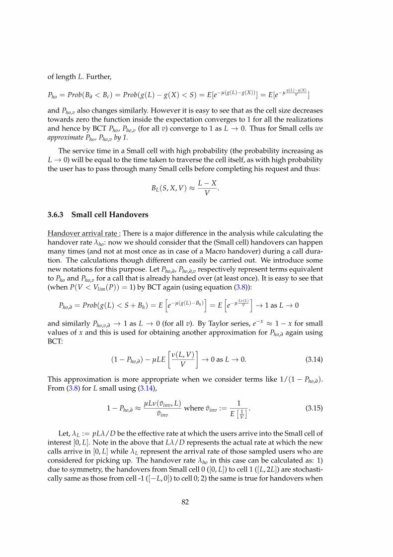
of length L. Further,

Pho = Prob(B∂ < Bc) = Prob(g(L)− g(X) < S) = E[e−µ(g(L)−g(X))] = E[e−µη(L)−η(X)

V ]

and Pho,v also changes similarly. However it is easy to see that as the cell size decreasestowards zero the function inside the expectation converges to 1 for all the realizationsand hence by BCT Pho, Pho,v (for all v) converge to 1 as L → 0. Thus for Small cells weapproximate Pho, Pho,v by 1.

The service time in a Small cell with high probability (the probability increasing asL → 0) will be equal to the time taken to traverse the cell itself, as with high probabilitythe user has to pass through many Small cells before completing his request and thus:

BL(S, X, V) ≈ L − X

V.

3.6.3 Small cell Handovers

Handover arrival rate : There is a major difference in the analysis while calculating thehandover rate λho: now we should consider that the (Small cell) handovers can happenmany times (and not at most once as in case of a Macro handover) during a call dura-tion. The calculations though different can easily be carried out. We introduce somenew notations for this purpose. Let Pho,∂, Pho,∂,v respectively represent terms equivalentto Pho and Pho,v for a call that is already handed over (at least once). It is easy to see that(when P(V < Vlim(P)) = 1) by BCT again (using equation (3.8)):

Pho,∂ = Prob(g(L) < S + Bh) = E[

e−µ(g(L)−Bh)]

= E[

e−µLν(L)

V

]

→ 1 as L → 0

and similarly Pho,v,∂ → 1 as L → 0 (for all v). By Taylor series, e−x ≈ 1 − x for smallvalues of x and this is used for obtaining another approximation for Pho,∂ again usingBCT:

(1 − Pho,∂)− µLE

[

ν(L, V)

V

]

→ 0 as L → 0. (3.14)

This approximation is more appropriate when we consider terms like 1/(1 − Pho,∂).From (3.8) for L small using (3.14),

1 − Pho,∂ ≈ µLν(vinv, L)

vinvwhere vinv :=

1E[ 1

V

] . (3.15)

Let, λL := pLλ/D be the effective rate at which the users arrive into the Small cell ofinterest [0, L]. Note in the above that Lλ/D represents the actual rate at which the newcalls arrive in [0, L] while λL represent the arrival rate of those sampled users who areconsidered for picking up. The handover rate λho in this case can be calculated as: 1)due to symmetry, the handovers from Small cell 0 ([0, L]) to cell 1 ([L, 2L]) are stochasti-cally same as those from cell -1 ([−L, 0]) to cell 0; 2) the same is true for handovers when

82

a mobile travels from right to left; 3) so, the handovers into a cell of interest (cell 0) arestochastically same as those that go out of the cell 0; 4) thus under the assumption thathandovers are Poisson in nature, the handover rate should satisfy the following fixedpoint equation:

λhLPho,∂ + λLPho = λhL.

Using the approximation in equation (3.15),

λhL =λLPho

1 − Pho,∂≈ λ

pvinv

Dµν(vinv, L). (3.16)

Remark 3.6.4. Note that L∗λhL

:= arg minL

λhL = L∗ν(vinv) and that for fixed velocities (when

V ≡ v) vinv = v. Thus for fixed velocities, interestingly for any value of p, the cell sizeoptimizing the the handover rate λhL (considering the Small cell drops) is the same one that isoptimal for NES as well as ES calls, obtained by neglecting the Small cell drops.

Handover Speed distribution: Note in equation (3.16) the expectation E[1/V] in the lastterm is w.r.t. to the distribution corresponding to the handover calls and hence oneneeds to calculate these distributions. The handover arrivals are either at 0 or at L withhalf probability and since we are considering the positive velocities without loss of generalitythe position is always at 0. The (Small cell) handover speed distribution, fh,V(v), (afterconsidering the drops at Small cells) once again satisfies another fixed point equationdue to the statistical similarity between the arrivals into and out of the cell 0. In Ap-pendix P, this fixed point equation is derived and the Small cell handover speed dis-tribution is shown to converge to uniform speed distribution as the cell size L tends tozero. Thus the (Small cell) handover arrivals have approximately uniform speed distribution.

3.6.5 Stability Factor

The stability factor ρ in a Small cell queue is calculated in Appendix P using the ap-proximations for small cell sizes and we obtain:

ρpico

(L) =(λL + λhL)b

(1)

K≈ λpL

KDµν(vinv, L). (3.17)

Define

L∗ν/L(v) := arg max

L

ν(v, L)

L.

Thus the optimal cell size for stability factor is,

L∗ρ,pico := arg min

Lρ

pico(L) = L∗

ν/L(vinv).

3.6.6 New Call Block Probability

The Small cell can be modeled by an M/G/K/K queue as in the previous section. LetPBusy,pico represent the probability that an arrival (a new or an handover call) finds all

83

the K servers busy in the Small cell. This probability can be calculated using the resultsfrom queuing theory as done in the previous section using Erlang Loss formula,

PBusy,pico(L) :=ρ

pico(L)K/K!

∑Kk=0 ρ

pico(L)k/k!

.

A new arrival is not picked up either with probability 1 − p when the BS intentionallydoes not consider it for picking up or with probability pPBusy,pico when all the serversare busy. Thus, the new call block probability for system when considering Small celldrops will be given by,

PB,pico(L) = (1 − p) + pPBusy,pico(L).

From the above the cell size optimizing the block probability PB,pico will be same as thatoptimizing PBusy,pico, which further is same as L∗

ρ,pico (using the logic as in section 3.3.9).Thus it is clear that, L∗

PB,pico = L∗ν/L(vinv) and from (3.17) this optimizer is a zero of

dρ

dL= c1

2L(η(L)− vinvBh)− L2η′(L)

(η(L)− vinvBh)2 ,

where c1 is an appropriate positive constant. Hence we have,Theorem 3.6.6.1. The cell size optimizing the block probability of the NES calls consideringthe possible drops at Small cell boundaries, when resources are reserved for handover calls byintensionally dropping some of the new arrivals, is given by,

L∗PB,pico

= L∗ρ,pico = L∗

ν/L =

2

Pdβ0

β+1β−1

2Pd0β

β−1 − vinvBh

1β−1

when β > 1

2d0evinv Bh−Pd0

2Pd0 when β = 1.

When this optimal cell size is compared at fixed velocities with that obtained afterneglecting the Small cell drops (that obtained in Theorem 3.3.7.1) we find that: 1) whenβ > 1, the two cell sizes matches except for a factor of ((β + 1)/(2β))1/(β−1); 2) whenβ = 1, the difference is in the power of the exponent, an extra −Pd0 factor for the cellsize with Small cell drops. This differences are negligible only when β is close to 1 (butnot equal to 1). The two systems use different call admission control mechanisms andhence the difference. Nevertheless the optimal cell size of the Theorem 3.6.6.1 is valid for adistributed call management system and further it gives the cell size even for velocity profileswith non zero variance.

3.6.7 Drop Probability

It was straight forward to calculate the drop probability for the previous case (i.e., with-out Small cell drops) as the drop could have occurred at maximum at one Macro bound-ary. It is more tedious to calculate the same when drops are also possible at Small cell

84

boundary. This tedious job is carried out in Appendix P, wherein the drop probabilityis obtained by conditioning on two events. We obtain (see Appendix P):

PD,pico =PBusy,pico

µ(η(L)−vinvBh)vinv

+ PBusy,pico

It is interesting to see that both the call drop and the new call block probabilities dependupon the busy probability PBusy,pico and one can thus design a optimal system (consid-ering Small cell drops) by minimizing the busy probability or equivalently the stabilityfactor ρ

pico. We thus propose to choose the optimal cell size:

L∗NES,pico := L∗

ρ,pico = L∗PB,pico,

which is obtained in Theorem 3.6.6.1.

3.7 Conclusions and Future work

We looked at the problem of characterizing the performance of Small cell networksin the presence of mobility. We modeled various traffic types between base-stationsand mobiles as different types of queues. We derived explicit expressions for expectedwaiting time, service time and drop/block probabilities for the various queuing modelsconsidered for both fixed as well as random velocity of mobiles. We showed that thereexists an optimal cell size for a given velocity profile, which minimizes the service timefor elastic applications as well as the drop and block probabilities of non-elastic appli-cations. We obtained (approximate) closed form expressions for this optimal cell sizewhen the velocity variations of the mobiles is very small. We find that if the call islong enough, the optimal cell size depends mainly on the velocity profile of the mo-biles, its mean and variance.; It is independent of the traffic type or duration of thecalls. We show that for any fixed power of transmission, there exists a maximum veloc-ity beyond which successful communication between the mobile and the system is notpossible. This maximum possible velocity increases with the power of transmission.Further, for any given power, the optimal cell size increases when either the mean orthe variance of the mobiles velocity increases.

The mobility models considered in this work are suitable for modeling users trav-eling continuously with considerable speeds (example users traveling in a car). Themovement of slower users (e.g., pedestrians) can be better captured by either RandomWalk or Random Way-point model. Still better would be to consider systems with het-erogeneous users (slow moving, fast moving and users that are at rest). We consideredtwo dimensional Small cell networks in [118] catering to non elastic users, in which theusers can move in any direction across the cell. In that work, we brought out someissues while designing the Small cell networks that are specific to two dimensional cel-lular networks. It would be interesting to extend those results for elastic users andfurther for heterogeneous users.

85

3.8 Appendix M: Calculations related to Macro queue

3.8.1 M.1 Proof of Theorem 3.3.3.1

The communication time is finite with probability one if and only if

Prob(Bh > g(L)) = Pn,V(VBh > η(L)) = 0, where η(L) := Vg(L).

Note from (3.3) that η is only a function of P, L and hence that this probability dependsonly upon the velocity profile V, cell size L and the transmit power P. Because of thepath loss, for any fixed P, η(L) increases as L increases and finally saturates (whenβ > 1). Thus for all L (when β > 1),

η(L) ≤ η∞ := limL→∞

η(L) < ∞.

When β = 1, η∞ = ∞ and this proves the first statement of the Theorem. As Prob(Bh >

g(L)) = Prob (VBh > η(L)), there exists a cell size L with P(Bh > g(L)) = 0 if and onlyif

Prob

(

V >η∞

Bh

)

= 0.

Thus with a given power P, the system can handle all velocities that are strictly lessthan

Vlim :=η∞

Bh=

2Pd0β

β − 1.

3.8.2 M.2 Moments of service time and its derivatives

The moments can be rewritten as,

b(k) =1

(1 + Pho)

∫ ∞

0

∫ D

−D

∫ Vmax

0

[


]

fn,V(v)dv fn,X(x)dx µe−µsds.

= En

[


1 + Pho

]

.

By Bounded Convergence Theorem (BCT), all b(k) are continuously differentiable(c.d.) in L and the derivative is

db(k)

dL= En

[

d

dL

(


1 + Pho

)]

86

because: 1) BD is almost surely c.d.; 2) Pho,v is c.d. everywhere in L; 3) Pho is c.d. and 4)all the derivatives involved are uniformly bounded almost surely; 4) hence by virtue ofmean value theorem, the terms like

|BD(X, V, S; L + δ)− BD(X, V, S; L)|δ

,|Pho,v(L + δ)− Pho,v(L)

δetc

can be bounded uniformly by a constant.

3.8.3 M.3 ν has an unique maximizer:

From equation (3.3), g and hence η = vg are both concave in L on (0, ∞) for every v.Thus from (3.8), for any fixed velocity v, ν has a unique maxima,

L∗ν(v) := arg max

Lν(v, L),

which satisfies ∂ν/∂L = 0 (as clearly L∗ν(v) > 0 for all v).

3.8.4 M.4 Derivatives db(k)/dL vanish only at L∗ν(v) when V ≡ v

Define Ψ(L) := En

[

BD(X, V, S)k + BD(−D, V, S)kPho,V

]

. Then from (3.11)

b(k) =Ψ(L)

1 + Pho.

From (3.4), Bc depends upon L only via the function ν given by (3.8) and hence so is theservice time BD(x, v, s) = minBc(v, s), B∂(x, v) for all x, v, s. Similarly from (3.10) and(3.9), Pho,v and Pho depend upon L only via the function ν. Hence with

Θ(v) := −∂Pho,v

∂ν=

µ

vEn,X

[

(D − X)e−µν(v,L)(D−X)/v]

db(k)

dL=

11 + Pho

En

[

∂ν(V, L)

∂L

(

∂BD(X, V, S)k

∂ν+ Pho,V

∂BD(−D, V, S)k

∂ν+

∂Pho,V

∂νBD(−D, V, S)k

)]

− 1(1 + Pho)2 Ψ(L)

dPho

dL

=1

1 + PhoEn

[

∂ν(V, L)

∂L

(

−kBD(X, V, S)k−1 S1SV<(D−X)ν(V,L)ν(V, L)2

− kPho,V BD(−D, V, S)k−1 S1SV<2Dν(V,L)ν(V, L)2 − BD(−D, V, S)kΘ(V)

)]

+1

(1 + Pho)2 Ψ(L)En

[

∂ν(V, L)

∂LΘ(V)

]

= En

∂ν(V, L)

∂L( −k

Sk1SV<(D−X)ν(V,L)ν(V,L)k+1 − kPho,V

Sk1SV<2Dν(V,L)ν(V,L)k+1 − BD(−D, V, S)kΘ(V)

1 + Pho

+Ψ(L)Θ(V)

(1 + Pho)2 )

. (3.18)

87

Thus the derivatives will have the form

db(k)

dL= En,V

[

∂ν(V, L)

∂LEn,X,S[Γ

(k)(X, V, S, ν(V, L))]

]

(3.19)

for some functions Γ(k). Thus for fixed velocities, i.e., when V ≡ v

db(k)

dL=

∂ν(v, L)

∂LEn,X,S[Γ

(k)(X, v, S, ν(v, L))]. (3.20)

Claim : The term En,X,S[Γ(k)(X, v, S, ν(v, L))] is strictly negative.

Proof of Claim: For any velocity v, BD(X, v, S) ≤ BD(−D, v, S) for all (X, S). Thus, forfixed velocities,

Ψ(L) ≤ (1 + Pho,v)En,S[BD(−D, v, S)k].

Further Pho = En,V [Pho,V ] = Pho,v. Hence the sum of the last two inner terms of theequation (3.18),

En,X,V

[

−BD(−D, V, S)kΘ(V)

1 + Pho+

Ψ(L)Θ(V)

(1 + Pho)2

]

≤ 0.

The remaining two inner terms of (3.18) are always negative and this proves the Claim.

From (3.20), by the virtue of the Claim, derivative db(k)/dL is zero only at a zero of∂ν/∂L. But ∂ν/∂L has a unique zero at the maximizer L∗

ν(v). Thus L∗ν(v) is the only

zero of all the service time moments.

3.9 Appendix P: Calculations for Small cell queue

3.9.1 P.1 Small cell Handover Speed Distribution

In the following the event ∂ arrival = ∂ means that the arrival in cell 0 was at theboundary (i.e., it was an handover arrival from cell -1), the event int arrival = intmeant a new arrival in cell 0 and the event ho implies the cell 0 active user has reachedthe next boundary before finishing his service (i.e, has to be handed over to cell 1). Notethat an handover from cell 0 occurs either due to an already handed over call or newcall, whose service could not be completed before reaching the (other) boundary of cell0 and thus:

Prob(ho) =λLPho + λhLPho,∂

λL + λhL.

88

Note that Prob(ho) → 1 as L → 0 (as both Pho, Pho,∂ converge to 1). With the abovenotations, the fixed point equation for the handover speed density can be obtained as:

fh,V(v) = Prob(V ∈ vdv|ho f rom cell 0)

= Prob(V ∈ vdv int arrival|ho) + Prob(V ∈ vdv ho arrival|ho)

=Prob(ho V ∈ vdv int) + Prob(V ∈ vdv ∂ ho)

Prob(ho)

=Prob(ho|int v)Prob(V ∈ vdv|int)Prob(int)

Prob(ho)

+Prob(ho|∂ v)Prob(V ∈ vdv|∂)Prob(∂)

Prob(ho)

=Pho,v fn,V(v)

Prob(ho)

λL

λL + λhL+

Pho,v,∂ fh,V(v)

Prob(ho)

λhL

λL + λhL

Solving (when fn,V(v) = 1/Vmax for all v ≤ Vmax) the handover speed density is,

fh,V(v) =

λL

Prob(ho)(λL+λhL)VmaxPho,v

1 − λhLPho,v,∂

Prob(ho)(λL+λhL)

Thus as L tends to zero (Pho,v, Pho,v,∂, Prob(ho), Pho → 1), the speed of an handover arrivalwill tend to uniform distribution. This effect is seen faster if the packet sizes S are larger.

3.9.2 P.2 Small cell Stability Factor

The stability factor ρ in a Small cell queue is given by:

ρpico

(L) =(λL + λhL)b

(1)

K=

1K

EV [λLEX[ES[BL(S, X, V)]] + λhLES[BL(S + Bh, 0, V)]]

≈ 1K(λL(L − E[X]) + LλhL) E

[

1V

]

=1K

(

λLL

2+ LλhL

)

E

[

1V

]

= c0L(λL + 2λhL)as Pho ≈ 1

≈ c0LλL1 − Pho,∂ + 2

1 − Pho,∂≈ 2c0λLL

1 − Pho,∂

where c0 = 1/(2K)E[1/V] is a constant independent of L. Using the approximation in(3.15),

ρpico

(L) =λpL

KDµν(vinv, L). (3.21)

3.9.3 P.3 Drop probability

The drop probability PD,pico considering possible Small cell drops can be calculated asbelow:

PD,pico = Prob( Call ever Dropped before completion| Call is picked up)

= Pho

(

Pho,D(1 − PBusy,pico) + PBusy,pico

)

+ (1 − Pho)(0)

89

where Pho,D is defined as the probability of call drop at any of the future instances ofhandovers, given that the current handover (first handover in the context of the aboveequation) is successful. Because of the memoryless nature of S, this probability doesnot depend upon the number of the handover. Probability Pho,D can be calculated byfirst conditioning on the event that the call is completed in the current cell (call it as C)and then on the event that the call is not picked up in the next cell (call it as S). Notethat Pho(Cc) = Pho,∂ and Pho(S|Cc) = Pho, f ail = 1 − PBusy,pico. Thus, by conditioning

Pho,D = Pho( Call dropped ∩ C) + Pho( Call dropped ∩ Cc)

= 0 + Pho,∂Pho( Call dropped |Cc)

= Pho,∂ (Pho( Call dropped ∩ S c|Cc) + Pho( Call dropped ∩ S|Cc))

= Pho,∂(

Pho,D(1 − PBusy,pico) + 1PBusy,pico

)

Solving=

PBusy,picoPho,∂

1 − Pho,∂(1 − PBusy,pico)and hence,

PD,pico =PhoPBusy,pico

1 − Pho,∂(1 − PBusy,pico)≈ PBusy,pico

1 − Pho,∂ + PBusy,pico. (3.22)

=PBusy,pico

µLν(vinv,L)vinv

+ PBusy,pico

=PBusy,pico

µ(η(L)−vinvBh)vinv

+ PBusy,pico

3.10 Publications

1. Veeraruna Kavitha, Sreenath Ramanath and Eitan Altman, "Spatial queuing anal-ysis for design and dimensioning of Picocell networks with mobile users", Else-viers Performance Evaluation, Volume 68, Issue 8.

2. Sreenath Ramanath, Veeraruna Kavitha, Eitan Altman, "Spatial queuing analysisfor mobility in pico cell networks", proceedings of WiOpt 2010, May 31-Jun 04,Avignon, France.

3. Sreenath Ramanath, Veeraruna Kavitha, Eitan Altman, "Impact of mobility oncall block, call drops and optimal cell size in small cell networks", proceedings ofthe Workshop on Indoor and Outdoor Femto Cells (IOFC’10), Sep 26, Istanbul,Turkey.

90

Chapter 4

Fair Assignment of Base StationLocations


4.2 Our model and assumptions . . . . . . . . . . . . . . . . . . . . . . . . 92

4.3 Large population limits and problem statement . . . . . . . . . . . . . 93

4.4 Analysis : Single BS Placement . . . . . . . . . . . . . . . . . . . . . . 96

4.5 Optimal and fair placement of a single BS . . . . . . . . . . . . . . . . 99

4.6 Optimal and fair placement of two BS in an outdoor cell . . . . . . . 106

4.7 Conclusions and future perspectives . . . . . . . . . . . . . . . . . . . 110

4.8 Appendix A : Large population limits - power, throughput and α-fairplacement of two base stations: . . . . . . . . . . . . . . . . . . . . . . 110

4.9 Publications . . . . . . . . . . . . . . . . . . . . . . . . . . . . . . . . . . 112

4.1 Introduction

In a cellular network, models used to derive analytic expressions for capacity, coverage,etc, often assume base station (BS) locations to be at the center of the cell. Such a modelbrings in a regular geometry to the problem being addressed and many a times resultsin closed-form analytic expressions for metrics of interest.

While, this indeed facilitates analysis, the actual throughput achievable at the BS,tends to vary significantly, depending on the BS placement and cell geometry. Theregular geometric model with a centrally located BS is a good model, when one assumesuniform density of users. But, today’s cellular networks have concentration of users, forexample hot-spots or indoor-outdoor partitions that offer various levels of attenuationto radio signals, not to mention the ever present channel fading and shadowing effectsabove this.

91

The goal of our research is to place the BS in a manner which is optimal for anygeneral fairness criterion; that of α-fairness [105, 147], which addresses popular fairnesscriterion like global, proportional, harmonic and max-min fairness. We show that theα-fair BS location varies continuously with fairness parameter α and moves close to thecenter of the cell as α increases asymptotically. This implies that, the regular geometricmodels (which place BS at the center) have max-min fair BS placement.

We further observe (via some numerical examples) that α-fair BS location variessignificantly based on system parameters like path-loss, noise variance. However weshow that the max-min fair BS placement is close to the center of the cell irrespective ofthe system parameters.

To bring in the importance of BS placement, we consider cells which are completelyoutdoors or which have indoor-outdoor partitions (Split cells). We consider cases whereuser density can be uniform or tend to increase along the cell (a simplistic model for ahot spot) [99]. We consider cases where adjacent cells can use the same frequency ordifferent frequencies. For the later case, we look at the problem of fair assignmentof two base stations (BS), where the cell gets divided into sub-cells from the users’perspective based on SINR association criteria. We limit our study to free space path-loss and the analysis with fading and shadowing would be our subsequent focus.

We derive simplified expressions for α-fair objective functions using large popula-tion limits , i.e., as the number of users become large. We use Strong Law of Large Num-bers (SLLN) to replace summation of large number of terms in the objective functionwith appropriate expected value almost surely (AS). The expected value is expressed asintegrals. Using these large population limits, we obtain both theoretical and numeri-cal results. The α-fair BS locations obtained are optimal for almost all realizations of theusers locations.

We begin our study by introducing our model and review the generalized α-fairfairness criterion in Section 4.2. In Section 4.3, we derive the α-fair placement crite-rion under large population limits. In Section 4.4, we analyze α-fair placement of basestations as α increases asymptotically and come across some interesting insights. InSection 4.5, we study the α-fair BS locations for the case of a) an outdoor cell and b) amixed partition cell (split-cell) via some numerical examples. Next, in Section 4.6, wederive the α-fair BS locations for an outdoor cell which has two BS. We conclude ourstudy in Section 4.7.

4.2 Our model and assumptions

Our focus is on communication in the uplink (UL) direction. Large number, N, of usersare located on i.i.d. locations on the line segment [−D, D]. The line segment is dividedinto cells of length L and one or more base stations, each of unit height, are placed inevery cell.

The placement of the BS(s) is the issue that we address in this work. One is usually

92

interested in maximizing global throughput (the sum throughput due to all users) ateach BS, i.e., place the BS(s) such that the global throughput is maximized. However,maximizing the global throughput can result in starving the users at a far away location,which in turn can reduce the network efficiency. Hence, several fairness criterion havebeen suggested and implemented in various network architectures ([105, 147]).

In [105] it is shown that all these fairness criterion are special cases of a generalizedfairness concept: the α-fairness . Given a positive constant α 6= 1, consider for examplethe problem of determining z so as to maximize

maxz∈[0,L]

∑xi∈[0,L]

θ(xi, z)1−α

1 − α(4.1)

where, θ(xi, z) is the throughput at the BS located at z from a user located at xi. Notethat the above objective function is defined over the convex set [0, L]. Further, when theobjective function is concave (we will show in later sections that this is the case most ofthe times) and the constraints are linear, this defines a unique allocation which we callthe α-fair allocation. It turns out that α-fairness gives global optimum for α → 0, pro-portional fairness when α → 1, harmonic (delay minimization) fairness indexHarmonicfairnessfor α = 2 and max-min fairness when α → ∞.

We begin our study by first deriving explicit expressions for power, throughput andα-fair placement criterion under large population limits (as the number of users becomelarge). Throughout the work, we use large population limits for analytical purposes.The idea is similar to fluid limits (see [90]), where summation of large number of termsis approximated by appropriate integrals.

4.3 Large population limits and problem statement

Large number, N, of users are located at Xii≤N , where the locations Xi of the usersare i.i.d., according to some probability measure P(dx) = λ(x)dx. We assume that eachuser uses the same power for transmission. Without loss of generality, the total power inthe system equals 1 and hence the power used by each user is 1/N.

We first consider the case of a single BS in the cell and compute the total powerreceived, throughput achievable and the α-fair placement for the BS under large popu-lation limits. The case of two base stations follows in a similar way and is addressed inAppendix.

4.3.1 Power computation :

The power received at a BS located at z from a user at Xi is given by,

P(Xi, z) =1N(1 + (z − Xi)

2)−β2 .

93

Thus the total power received at the BS is

Ptot(z) =N

∑i=1

P(Xi, z) =1N

N

∑i=1

(1 + (z − Xi)2)

−β2 .

This is a random power. By the Strong Law of Large Number (SLLN) this convergesP-a.s. to a constant limit

limN→∞

Ptot(z) = E[

(1 + (z − Xi)2)

−β2

]

=∫ D

−D(1 + (z − x)2)

−β2 λ(x)dx. (4.2)

Hence for large values of N one can approximate Ptot(z) almost surely with the aboveintegral.

4.3.2 Throughput computation:

The signal to interference noise ratio (SINR) at the BS located at z from a user at Xi is

SINR(Xi, z) =P(Xi, z)

σ2 + Ptot(z)− P(Xi, z),

where σ2 is the noise variance. In the above, Ptot(z) is approximated P−almost surelyby a constant value, i.e., by the integral of (4.2). However SINR(Xi, z) is still randombecause of the term P(Xi, z). The Shannon capacity or throughput achievable at the BSlocated at z from a user at Xi is

θ(Xi, z) = log (1 + SINR(Xi, z))

Considering a receiver with an adapted filter and using the approximation log(1 +x) ≈ x (for smaller values of x), the throughput achievable is

θ(Xi, z) =P(Xi, z)

σ2 + Ptot(z)− P(Xi, z)

The total (global) throughput achievable at the BS from all the users in the cell ofinterest is:

f (z) =N

∑i=1

1Xi∈[0,L]θ(Xi, z)

=1N

N

∑i=1

1Xi∈[0,L](1 + (z − Xi)

2)−β2

σ2 + Ptot(z)− P(Xi, z)

≈ 1N

N

∑i=1

1Xi∈[0,L](1 + (z − Xi)

2)−β2

σ2 + Ptot(z),

94

as for large values of N, P(Xi, z) is negligible in comparison with Ptot(z). Again, theabove Random sum can be approximated using Strong Law of Large Numbers when-ever the number of users inside the cell is large P-almost surely, giving rise to the fol-lowing large population approximation:

f (z) ≈ E[

IX1∈[0,L]ψ(X1, z)]

=∫ L

0ψ(x, z)λ(x)dx with (4.3)

ψ(x, z) :=(1 + (z − x)2)

−β2

σ2 + Ptot(z).

4.3.3 α-fair placement criterion :

The α-fair objective function of (4.1) in a similar way can be approximated almost surelyunder large population limits by:

fα(z) := Nα 11 − α

∫ L

0ψ(x, z)(1−α)λ(x)dx

Thus α-fair placement of the BS is given by,

z∗(α) = arg maxz

fα(z)

= arg maxz

fα(z) where (4.4)

fα(z) :=1

1 − α

∫ L

0ψ(x, z)(1−α)λ(x)dx.

Important point to note here is that, for almost all realizations of the locations of the usersthe objective function is approximated by the constant integral and hence z∗(α) is optimal α-fairlocation for almost all users locations.

4.3.4 Problem statement

Now with this background, we pose the following problems:

1. Find BS location z so as to maximize global throughput f (z). See large populationlimit (4.3).

2. Find the α-fair BS location z∗ which maximizes fα(z) for various fairness criterion.See large population limit (4.4)

In subsequent sections, we analyze and apply the α-fair placement criterion to ob-tain BS locations which are both optimal and fair in various cellular environments con-sidered.

95

4.4 Analysis : Single BS Placement

We notice that both the global throughput (large population limit (4.3)) and the α-fairplacement (large population limit (4.4)) of the BS is dependent on the total power re-ceived Ptot(z) at the BS, which in-turn depends on its location z. In many cases, thetotal-power received can be assumed independent of the location of the BS, wheneverthe cell size is small (which is typical of pico cells). This for example is true for cells

with user density λ(x) being symmetric aboutL

2(uniform being the trivial case) and

completely located outdoors.

The above assumption simplifies analysis to a good extent and is considered in thefirst subsection, while an approximate analysis is given in the following subsectionwithout this assumption.

We consider asymptotic analysis in this section and hence consider only the caseswith α > 1. For notational simplicities, we redefine fα(z) of equation (4.4) after drop-ping the division by (1 − α) factor and now,

z∗(α) := arg maxz∈[0,L]

(− fα(z)) .

4.4.1 Ptot(z) is independent of BS location z :

As Ptot(z) is independent of z, the α-fair location is obtained by minimizing the function,

fα(z) :=∫ L

0

(

1 + (z − x)2)−β2 (1−α)

λ(x)dx

We can easily show that fα(z) is concave in z. We also have joint continuity in (α, z) byBounded Convergence theorem. Hence, by maximum theorem [137] under convexity,we getLemma 4.4.2. The function z∗(α) is continuous in α.

By differentiability of fα(.),

g(α, z∗(α)) = 0.

where with γ :=β

2(α − 1)− 1 (for some appropriate c 6= 0),

g(α, z) := c∂ fα(z)

∂z

=∫ L

0(z − x)

(

1 + (z − x)2)γλ(x)dx.

96

If z <L

2then,

(

1 +(

L

2

)2)−γ

g(α, z) =∫ L

2 +z

0(z − x)

(

1 + (z − x)2

1 + ( L2 )

2

)γ

λ(x)dx

+∫ L

L2 +z

(z − x)

(

1 + (z − x)2

1 + ( L2 )

2

)γ

λ(x)dx

tends to −∞ as α ↑ ∞, because the first term tends to zero while the later tends to −∞

(by bounded convergence theorem). Therefore there exists α0 > 0 such that, g(α, z) < 0and hence such that,

g(α, z) 6= 0 for all α > α0.

Similarly if z >L

2then,

(

1 +(

L

2

)2)−γ

g(α, z) tends to ∞ as α ↑ ∞ and hence we

have,

g(α, z) 6= 0 for all α > α0(z) whenever z 6= L

2.

However

(

1 +(

L

2

)2)−γ

g

(

α,L

2

)

→ 0 as α ↑ ∞.

In fact, we have (by monotonicity arguments) for all z0 <L

2:

g(α, z) 6= 0 for all α > α0(z0), z ∈ [0, z0] ∪ [L − z0, L],

and hence the optimizer lies in a smaller interval aroundL

2for all larger values of α and

thus we get the following:

Lemma 4.4.3. For every ǫ <L

2there exists an α0(ǫ) (depending upon ǫ), such that for all

α > α0(ǫ)

z∗(α) ∈[

L

2− ǫ,

L

2+ ǫ

]

.

i.e, the optimizer lies in a smaller interval aroundL

2for all larger values of α. That is, z∗α(z) →

L

2as α → ∞.

Whenever the density λ(x) is symmetric aboutL

2within the cell [0, L], using similar

derivative arguments one can get,Lemma 4.4.4. The partial derivatives under symmetric conditions, for all α

∂ fα(z)

∂α

∣

∣

∣

∣

z=z0

= 0

and hence optimal locations for all α are atL

2.

97

Summary of the results :

1. α-fair location is continuous in α (by Lemma 4.4.2).

2. When the density function λ is symmetric aboutL

2then by Lemma 4.4.4 all the

α-fair locations are at the center of the cell.

3. If density is not symmetric aboutL

2then, by Lemma 4.4.3, the α-fair locations

tend toL

2as α tends to infinity.

4. Lemma 4.4.3, 4.4.4 are correct as long as the support of measure λ contains both

the end points, i.e., 0, L ⊂ supp(λ). If not, the same results are true withL

2replaced

with length(supp(λ))/2.

4.4.5 Ptot(z) is dependent on BS location z :

Next, we consider cases when the total power Ptot(z) is dependent on base station lo-cation z. This is true for cases with non-symmetric user densities, cells with partitions,etc.

Let h(.; z) represent the following parametrized function :

h(x; z) :=(

σ2 + Ptot(z)) (

1 + (x − z)2)β2 .

and let ||h(.; z)||p represent its Lp norm with respect to the probability measureλ(x)dx∫ L

0 λ(x)dx.

With the above definitions, for α > 1, we can equivalently write the optimal α-fairlocation as,

z∗(α) = arg minz∈[0,L]

||h(.; z)||α−1.

As α → ∞, ||h(.; z)||α−1 → ||h(.; z)||∞ and one can show that,

limα→∞

z∗(α) ≈ arg minz∈[0,L]

||h(.; z)||∞.

Since,

||h(.; z)||∞ =(

σ2 + Ptot(z))

supx∈[0,L]

(

1 + (x − z)2)β2

=(

σ2 + Ptot(z))

(

1 + (maxz, L − z)2)

β2

=(

σ2 + Ptot(z))

max(1 + z2)β2 , (1 + (L − z)2)

β2 ,

98

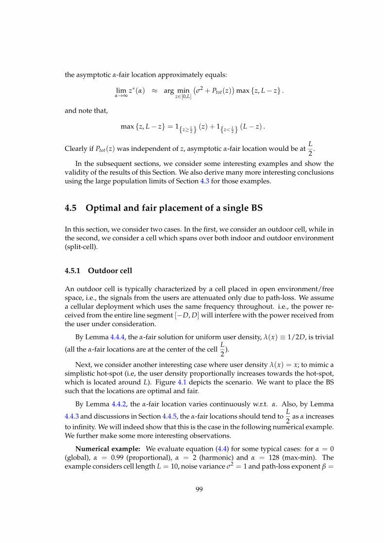
the asymptotic α-fair location approximately equals:

limα→∞

z∗(α) ≈ arg minz∈[0,L]

(

σ2 + Ptot(z))

max z, L − z .

and note that,

max z, L − z = 1z≥ L2 (z) + 1z< L

2 (L − z) .

Clearly if Ptot(z) was independent of z, asymptotic α-fair location would be atL

2.

In the subsequent sections, we consider some interesting examples and show thevalidity of the results of this Section. We also derive many more interesting conclusionsusing the large population limits of Section 4.3 for those examples.

4.5 Optimal and fair placement of a single BS

In this section, we consider two cases. In the first, we consider an outdoor cell, while inthe second, we consider a cell which spans over both indoor and outdoor environment(split-cell).

4.5.1 Outdoor cell

An outdoor cell is typically characterized by a cell placed in open environment/freespace, i.e., the signals from the users are attenuated only due to path-loss. We assumea cellular deployment which uses the same frequency throughout. i.e., the power re-ceived from the entire line segment [−D, D] will interfere with the power received fromthe user under consideration.

By Lemma 4.4.4, the α-fair solution for uniform user density, λ(x) ≡ 1/2D, is trivial

(all the α-fair locations are at the center of the cellL

2).

Next, we consider another interesting case where user density λ(x) = x; to mimic asimplistic hot-spot (i.e, the user density proportionally increases towards the hot-spot,which is located around L). Figure 4.1 depicts the scenario. We want to place the BSsuch that the locations are optimal and fair.

By Lemma 4.4.2, the α-fair location varies continuously w.r.t. α. Also, by Lemma

4.4.3 and discussions in Section 4.4.5, the α-fair locations should tend toL

2as α increases

to infinity. We will indeed show that this is the case in the following numerical example.We further make some more interesting observations.

Numerical example: We evaluate equation (4.4) for some typical cases: for α = 0(global), α = 0.99 (proportional), α = 2 (harmonic) and α = 128 (max-min). Theexample considers cell length L = 10, noise variance σ2 = 1 and path-loss exponent β =

99

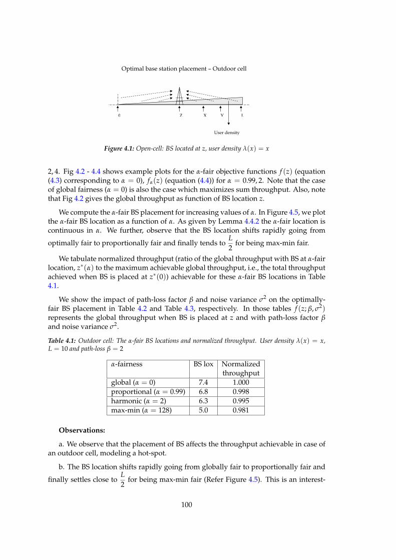
0 L Z X Y

Figure 4.1: Open-cell: BS located at z, user density λ(x) = x

2, 4. Fig 4.2 - 4.4 shows example plots for the α-fair objective functions f (z) (equation(4.3) corresponding to α = 0), fα(z) (equation (4.4)) for α = 0.99, 2. Note that the caseof global fairness (α = 0) is also the case which maximizes sum throughput. Also, notethat Fig 4.2 gives the global throughput as function of BS location z.

We compute the α-fair BS placement for increasing values of α. In Figure 4.5, we plotthe α-fair BS location as a function of α. As given by Lemma 4.4.2 the α-fair location iscontinuous in α. We further, observe that the BS location shifts rapidly going from

optimally fair to proportionally fair and finally tends toL

2for being max-min fair.

We tabulate normalized throughput (ratio of the global throughput with BS at α-fairlocation, z∗(α) to the maximum achievable global throughput, i.e., the total throughputachieved when BS is placed at z∗(0)) achievable for these α-fair BS locations in Table4.1.

We show the impact of path-loss factor β and noise variance σ2 on the optimally-fair BS placement in Table 4.2 and Table 4.3, respectively. In those tables f (z; β, σ2)represents the global throughput when BS is placed at z and with path-loss factor βand noise variance σ2.

Table 4.1: Outdoor cell: The α-fair BS locations and normalized throughput. User density λ(x) = x,L = 10 and path-loss β = 2

α-fairness BS lox Normalizedthroughput

global (α = 0) 7.4 1.000proportional (α = 0.99) 6.8 0.998harmonic (α = 2) 6.3 0.995max-min (α = 128) 5.0 0.981

Observations:

a. We observe that the placement of BS affects the throughput achievable in case ofan outdoor cell, modeling a hot-spot.

b. The BS location shifts rapidly going from globally fair to proportionally fair and

finally settles close toL

2for being max-min fair (Refer Figure 4.5). This is an interest-

100

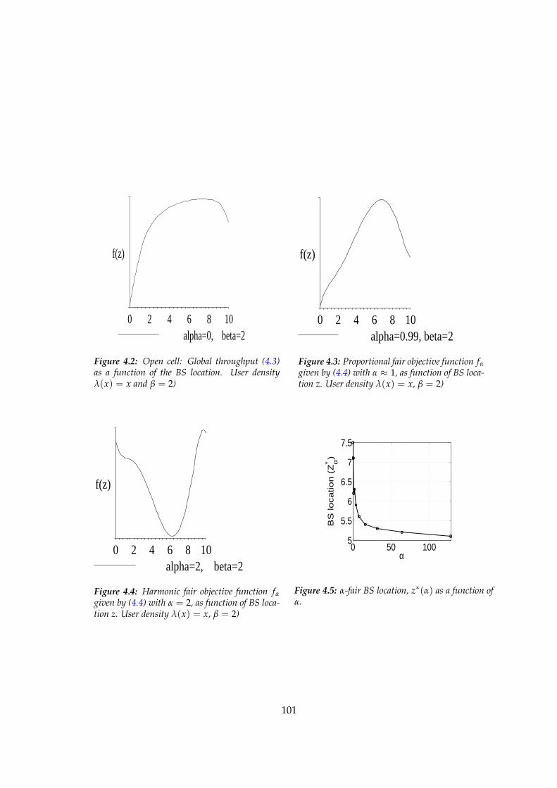
64 820

f(z)

10alpha=0, beta=2

Figure 4.2: Open cell: Global throughput (4.3)as a function of the BS location. User densityλ(x) = x and β = 2)

642

f(z)

0 108alpha=0.99, beta=2

Figure 4.3: Proportional fair objective function fα

given by (4.4) with α ≈ 1, as function of BS loca-tion z. User density λ(x) = x, β = 2)

6420

f(z)

108alpha=2, beta=2

Figure 4.4: Harmonic fair objective function fα

given by (4.4) with α = 2, as function of BS loca-tion z. User density λ(x) = x, β = 2)

0 50 1005

5.5

6

6.5

7

7.5

α

BS

lo

ca

tio

n (

Zα*)

Figure 4.5: α-fair BS location, z∗(α) as a function ofα.

101

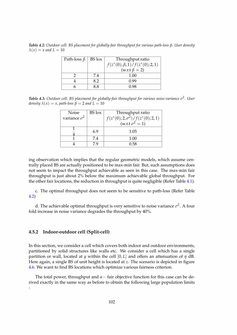
Table 4.2: Outdoor cell: BS placement for globally-fair throughput for various path-loss β. User densityλ(x) = x and L = 10

Path-loss β BS lox Throughput ratiof (z∗(0); β, 1)/ f (z∗(0); 2, 1)

(w.r.t β = 2)2 7.4 1.004 8.2 0.996 8.8 0.98

Table 4.3: Outdoor cell: BS placement for globally-fair throughput for various noise-variance σ2. Userdensity λ(x) = x, path-loss β = 2 and L = 10

Noise BS lox Throughput ratiovariance σ2 f (z∗(0); 2, σ2)/ f (z∗(0); 2, 1)

(w.r.t σ2 = 1)14

6.9 1.05

1 7.4 1.004 7.9 0.58

ing observation which implies that the regular geometric models, which assume cen-trally placed BS are actually positioned to be max-min fair. But, such assumptions doesnot seem to impact the throughput achievable as seen in this case. The max-min fairthroughput is just about 2% below the maximum achievable global throughput. Forthe other fair locations, the reduction in throughput is quite negligible (Refer Table 4.1).

c. The optimal throughput does not seem to be sensitive to path-loss (Refer Table4.2)

d. The achievable optimal throughput is very sensitive to noise variance σ2. A fourfold increase in noise variance degrades the throughput by 40%.

4.5.2 Indoor-outdoor cell (Split-cell)

In this section, we consider a cell which covers both indoor and outdoor environments,partitioned by solid structures like walls etc. We consider a cell which has a singlepartition or wall, located at y within the cell [0, L] and offers an attenuation of η dB.Here again, a single BS of unit height is located at z. The scenario is depicted in figure4.6. We want to find BS locations which optimize various fairness criterion.

The total power, throughput and α− fair objective function for this case can be de-rived exactly in the same way as before to obtain the following large population limits:

102

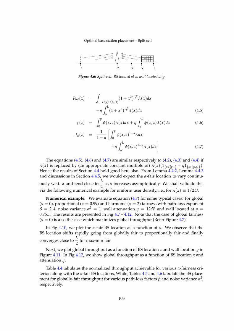
0 L Z X Y

Figure 4.6: Split-cell: BS located at z, wall located at y

Ptot(z) =∫

[−D,y)∪[L,D)(1 + x2)

−β2 λ(x)dx

+η∫ L

y(1 + x2)

−β2 λ(x)dx (4.5)

f (z) =∫ y

0ψ(x, z)λ(x)dx + η

∫ L

yψ(x, z)λ(x)dx (4.6)

fα(z) =1

1 − α

[

∫ y

0ψ(x, z)1−αλdx

+η∫ L

yψ(x, z)1−αλ(x)dx

]

(4.7)

The equations (4.5), (4.6) and (4.7) are similar respectively to (4.2), (4.3) and (4.4) ifλ(x) is replaced by (an appropriate constant multiple of) λ(x)(1x/∈[y,L] + η1x∈[y,L]).Hence the results of Section 4.4 hold good here also. From Lemma 4.4.2, Lemma 4.4.3and discussions in Section 4.4.5, we would expect the α-fair location to vary continu-

ously w.r.t. α and tend close toL

2as α increases asymptotically. We shall validate this

via the following numerical example for uniform user density, i.e., for λ(x) ≡ 1/2D.

Numerical example: We evaluate equation (4.7) for some typical cases: for global(α = 0), proportional (α = 0.99) and harmonic (α = 2) fairness with path-loss exponentβ = 2, 4, noise variance σ2 = 1 ,wall attenuation η = 12dB and wall located at y =0.75L. The results are presented in Fig 4.7 - 4.12. Note that the case of global fairness(α = 0) is also the case which maximizes global throughput (Refer Figure 4.7).

In Fig 4.10, we plot the α-fair BS location as a function of α. We observe that theBS location shifts rapidly going from globally fair to proportionally fair and finally

converges close toL

2for max-min fair.

Next, we plot global throughput as a function of BS location z and wall location y inFigure 4.11. In Fig 4.12, we show global throughput as a function of BS location z andattenuation η.

Table 4.4 tabulates the normalized throughput achievable for various α-fairness cri-terion along with the α-fair BS locations, While, Tables 4.5 and 4.6 tabulate the BS place-ment for globally-fair throughput for various path-loss factors β and noise variance σ2,respectively.

103

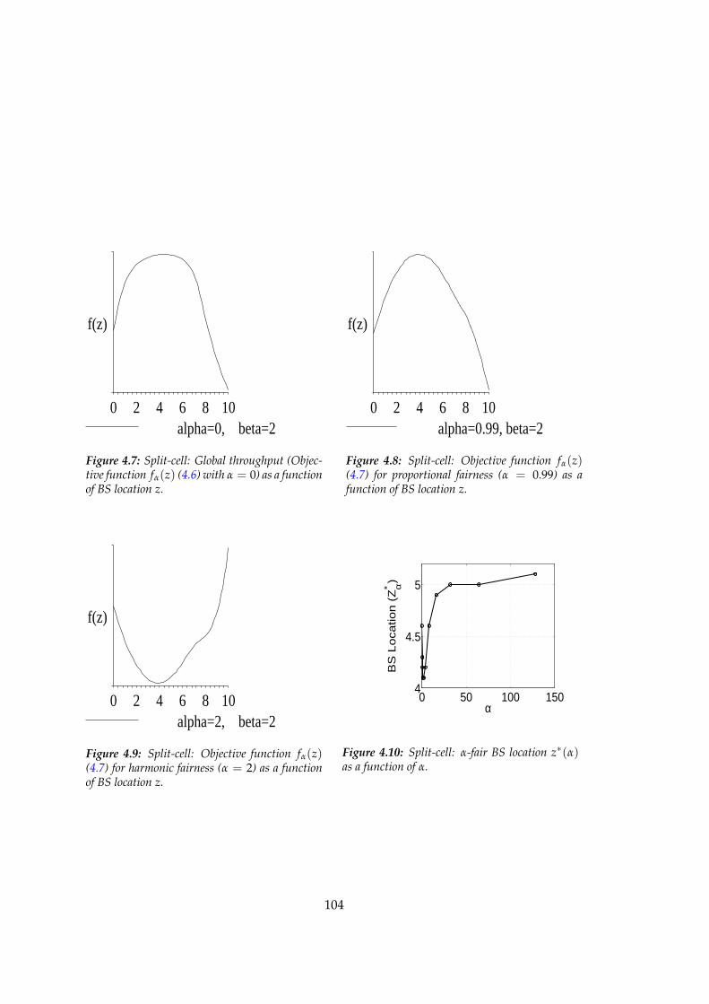
642

f(z)

0 108alpha=0, beta=2

Figure 4.7: Split-cell: Global throughput (Objec-tive function fα(z) (4.6) with α = 0) as a functionof BS location z.

642

f(z)

0 108alpha=0.99, beta=2

Figure 4.8: Split-cell: Objective function fα(z)(4.7) for proportional fairness (α = 0.99) as afunction of BS location z.

64 820

f(z)

10alpha=2, beta=2

Figure 4.9: Split-cell: Objective function fα(z)(4.7) for harmonic fairness (α = 2) as a functionof BS location z.

0 50 100 1504

4.5

5

α

BS

Lo

catio

n (

Zα*)

Figure 4.10: Split-cell: α-fair BS location z∗(α)as a function of α.

104

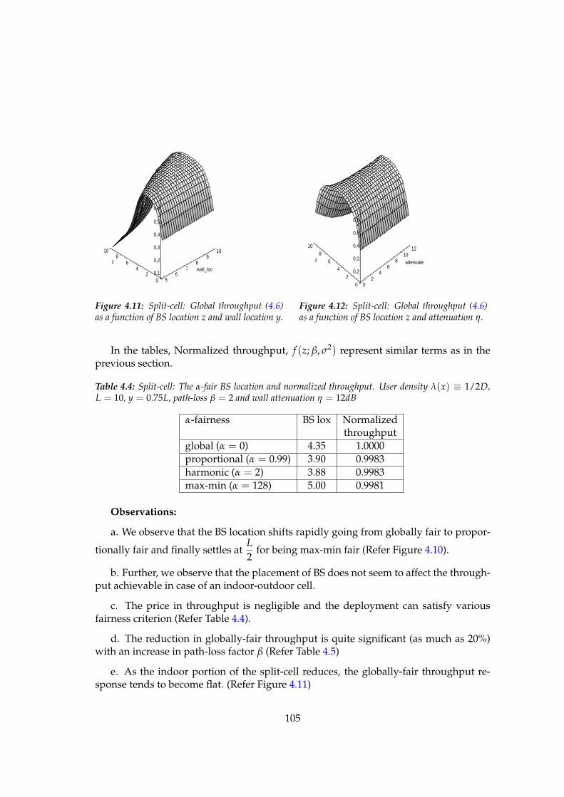
10 108 9

z 6 874 wall_loc

6250

0,1

0,2

0,3

0,4

0,5

0,6

Figure 4.11: Split-cell: Global throughput (4.6)as a function of BS location z and wall location y.

10 128 10

z 86 attenuate64

42 2

0 0

0,2

0,3

0,4

0,5

0,6

Figure 4.12: Split-cell: Global throughput (4.6)as a function of BS location z and attenuation η.

In the tables, Normalized throughput, f (z; β, σ2) represent similar terms as in theprevious section.

Table 4.4: Split-cell: The α-fair BS location and normalized throughput. User density λ(x) ≡ 1/2D,L = 10, y = 0.75L, path-loss β = 2 and wall attenuation η = 12dB

α-fairness BS lox Normalizedthroughput

global (α = 0) 4.35 1.0000proportional (α = 0.99) 3.90 0.9983harmonic (α = 2) 3.88 0.9983max-min (α = 128) 5.00 0.9981

Observations:

a. We observe that the BS location shifts rapidly going from globally fair to propor-

tionally fair and finally settles atL

2for being max-min fair (Refer Figure 4.10).

b. Further, we observe that the placement of BS does not seem to affect the through-put achievable in case of an indoor-outdoor cell.

c. The price in throughput is negligible and the deployment can satisfy variousfairness criterion (Refer Table 4.4).

d. The reduction in globally-fair throughput is quite significant (as much as 20%)with an increase in path-loss factor β (Refer Table 4.5)

e. As the indoor portion of the split-cell reduces, the globally-fair throughput re-sponse tends to become flat. (Refer Figure 4.11)

105

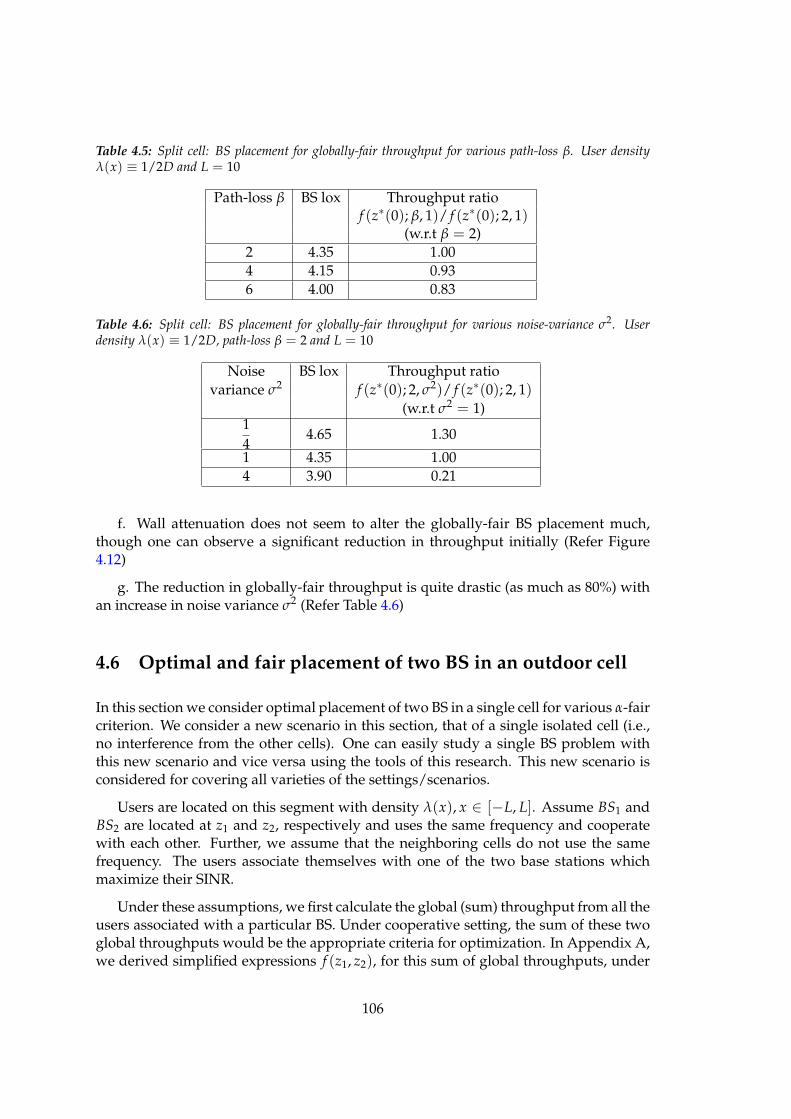
Table 4.5: Split cell: BS placement for globally-fair throughput for various path-loss β. User densityλ(x) ≡ 1/2D and L = 10

Path-loss β BS lox Throughput ratiof (z∗(0); β, 1)/ f (z∗(0); 2, 1)

(w.r.t β = 2)2 4.35 1.004 4.15 0.936 4.00 0.83

Table 4.6: Split cell: BS placement for globally-fair throughput for various noise-variance σ2. Userdensity λ(x) ≡ 1/2D, path-loss β = 2 and L = 10

Noise BS lox Throughput ratiovariance σ2 f (z∗(0); 2, σ2)/ f (z∗(0); 2, 1)

(w.r.t σ2 = 1)14

4.65 1.30

1 4.35 1.004 3.90 0.21

f. Wall attenuation does not seem to alter the globally-fair BS placement much,though one can observe a significant reduction in throughput initially (Refer Figure4.12)

g. The reduction in globally-fair throughput is quite drastic (as much as 80%) withan increase in noise variance σ2 (Refer Table 4.6)

4.6 Optimal and fair placement of two BS in an outdoor cell

In this section we consider optimal placement of two BS in a single cell for various α-faircriterion. We consider a new scenario in this section, that of a single isolated cell (i.e.,no interference from the other cells). One can easily study a single BS problem withthis new scenario and vice versa using the tools of this research. This new scenario isconsidered for covering all varieties of the settings/scenarios.

Users are located on this segment with density λ(x), x ∈ [−L, L]. Assume BS1 andBS2 are located at z1 and z2, respectively and uses the same frequency and cooperatewith each other. Further, we assume that the neighboring cells do not use the samefrequency. The users associate themselves with one of the two base stations whichmaximize their SINR.

Under these assumptions, we first calculate the global (sum) throughput from all theusers associated with a particular BS. Under cooperative setting, the sum of these twoglobal throughputs would be the appropriate criteria for optimization. In Appendix A,we derived simplified expressions f (z1, z2), for this sum of global throughputs, under

106

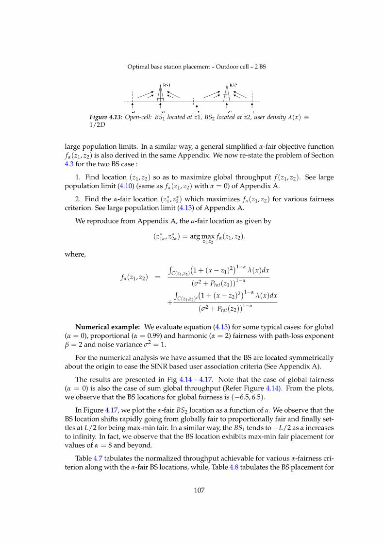
Figure 4.13: Open-cell: BS1 located at z1, BS2 located at z2, user density λ(x) ≡1/2D

large population limits. In a similar way, a general simplified α-fair objective functionfα(z1, z2) is also derived in the same Appendix. We now re-state the problem of Section4.3 for the two BS case :

1. Find location (z1, z2) so as to maximize global throughput f (z1, z2). See largepopulation limit (4.10) (same as fα(z1, z2) with α = 0) of Appendix A.

2. Find the α-fair location (z∗1 , z∗2) which maximizes fα(z1, z2) for various fairnesscriterion. See large population limit (4.13) of Appendix A.

We reproduce from Appendix A, the α-fair location as given by

(z∗1α, z∗2α) = arg maxz1,z2

fα(z1, z2).

where,

fα(z1, z2) =

∫

C(z1,z2)

(

1 + (x − z1)2)1−α

λ(x)dx

(σ2 + Ptot(z1))1−α

+

∫

C(z1,z2)c

(

1 + (x − z2)2)1−α

λ(x)dx

(σ2 + Ptot(z2))1−α

Numerical example: We evaluate equation (4.13) for some typical cases: for global(α = 0), proportional (α = 0.99) and harmonic (α = 2) fairness with path-loss exponentβ = 2 and noise variance σ2 = 1.

For the numerical analysis we have assumed that the BS are located symmetricallyabout the origin to ease the SINR based user association criteria (See Appendix A).

The results are presented in Fig 4.14 - 4.17. Note that the case of global fairness(α = 0) is also the case of sum global throughput (Refer Figure 4.14). From the plots,we observe that the BS locations for global fairness is (−6.5, 6.5).

In Figure 4.17, we plot the α-fair BS2 location as a function of α. We observe that theBS location shifts rapidly going from globally fair to proportionally fair and finally set-tles at L/2 for being max-min fair. In a similar way, the BS1 tends to −L/2 as α increasesto infinity. In fact, we observe that the BS location exhibits max-min fair placement forvalues of α = 8 and beyond.

Table 4.7 tabulates the normalized throughput achievable for various α-fairness cri-terion along with the α-fair BS locations, while, Table 4.8 tabulates the BS placement for

107

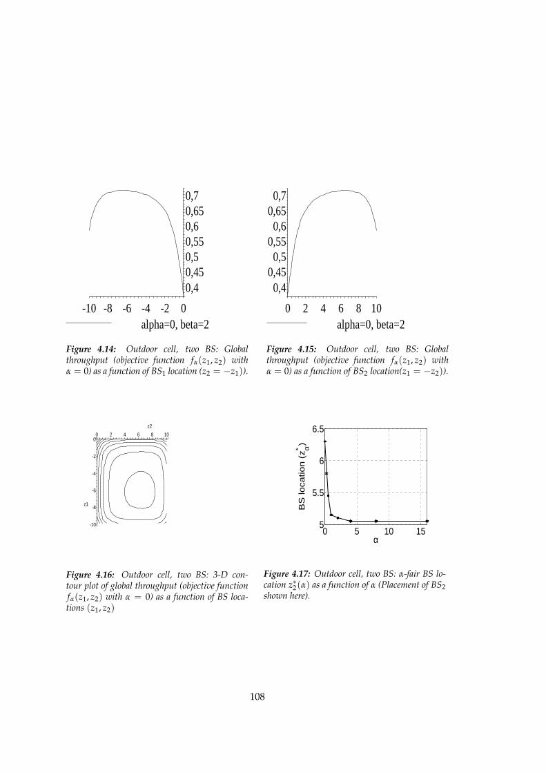
-4-6-8-10

0,70,650,60,550,50,450,4

0-2alpha=0, beta=2

Figure 4.14: Outdoor cell, two BS: Globalthroughput (objective function fα(z1, z2) withα = 0) as a function of BS1 location (z2 = −z1)).

6420

0,70,65

0,60,55

0,50,45

0,4

108alpha=0, beta=2

Figure 4.15: Outdoor cell, two BS: Globalthroughput (objective function fα(z1, z2) withα = 0) as a function of BS2 location(z1 = −z2)).

-10

-8z1

-6

-4

-2

02 6 10840

z2

Figure 4.16: Outdoor cell, two BS: 3-D con-tour plot of global throughput (objective functionfα(z1, z2) with α = 0) as a function of BS loca-tions (z1, z2)

0 5 10 155

5.5

6

6.5

α

BS

loca

tion

(z α*

)

Figure 4.17: Outdoor cell, two BS: α-fair BS lo-cation z∗2(α) as a function of α (Placement of BS2shown here).

108

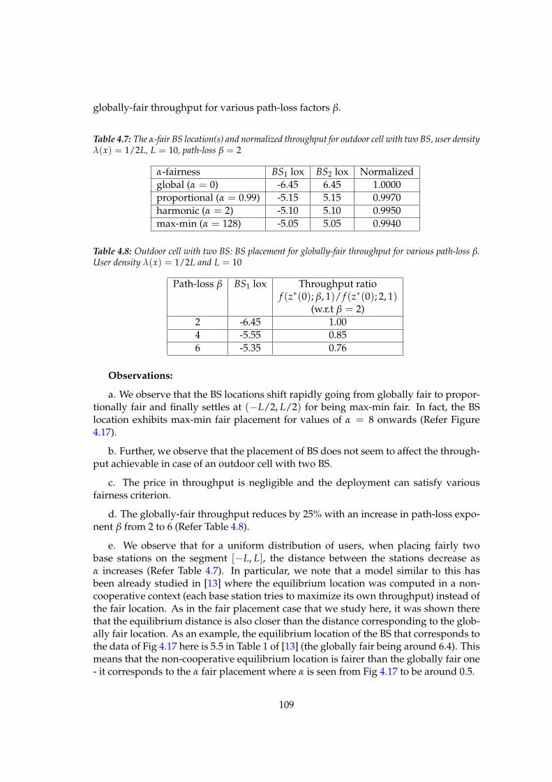
globally-fair throughput for various path-loss factors β.

Table 4.7: The α-fair BS location(s) and normalized throughput for outdoor cell with two BS, user densityλ(x) = 1/2L, L = 10, path-loss β = 2

α-fairness BS1 lox BS2 lox Normalizedglobal (α = 0) -6.45 6.45 1.0000proportional (α = 0.99) -5.15 5.15 0.9970harmonic (α = 2) -5.10 5.10 0.9950max-min (α = 128) -5.05 5.05 0.9940

Table 4.8: Outdoor cell with two BS: BS placement for globally-fair throughput for various path-loss β.User density λ(x) = 1/2L and L = 10

Path-loss β BS1 lox Throughput ratiof (z∗(0); β, 1)/ f (z∗(0); 2, 1)

(w.r.t β = 2)2 -6.45 1.004 -5.55 0.856 -5.35 0.76

Observations:

a. We observe that the BS locations shift rapidly going from globally fair to propor-tionally fair and finally settles at (−L/2, L/2) for being max-min fair. In fact, the BSlocation exhibits max-min fair placement for values of α = 8 onwards (Refer Figure4.17).

b. Further, we observe that the placement of BS does not seem to affect the through-put achievable in case of an outdoor cell with two BS.

c. The price in throughput is negligible and the deployment can satisfy variousfairness criterion.

d. The globally-fair throughput reduces by 25% with an increase in path-loss expo-nent β from 2 to 6 (Refer Table 4.8).

e. We observe that for a uniform distribution of users, when placing fairly twobase stations on the segment [−L, L], the distance between the stations decrease asα increases (Refer Table 4.7). In particular, we note that a model similar to this hasbeen already studied in [13] where the equilibrium location was computed in a non-cooperative context (each base station tries to maximize its own throughput) instead ofthe fair location. As in the fair placement case that we study here, it was shown therethat the equilibrium distance is also closer than the distance corresponding to the glob-ally fair location. As an example, the equilibrium location of the BS that corresponds tothe data of Fig 4.17 here is 5.5 in Table 1 of [13] (the globally fair being around 6.4). Thismeans that the non-cooperative equilibrium location is fairer than the globally fair one- it corresponds to the α fair placement where α is seen from Fig 4.17 to be around 0.5.

109

Further, our work can be extended to find the α-fair BS locations when multiple BSare to be located on a line segment or on a 2D grid. This is a step towards optimalBS placement to satisfy various fairness criteria when a macro-cell is divided into anumber of small cells. For example, the optimal placement of BS in pico-cell networks.

4.7 Conclusions and future perspectives

We studied the problem of optimal BS placement, optimal for various α-fair criterionin cellular networks. We considered simple 1D models which characterize both indoorand outdoor cellular environments with mixed partitions. We derived explicit expres-sions for α-fair criterion under large population limits. These limits were used to obtainthe theoretical asymptotic analysis of the α-fair locations. We show that the α-fair lo-cations converge close to center of the cell as α increases to infinity (which basicallyrepresents the max-min fair location).

The large population limits were also used to numerically compute BS locationswhich satisfy global, proportional, harmonic and max-min fairness. For the modelsconsidered, we presented results via plots and tables to show the variations in achiev-able throughput for the different fairness criterion. We also confirmed, via numericalexamples, that the α-fair locations converge to the center of the cell as α tends to infinity.

We next considered a two base station optimal placement problem again for vari-ous α-fair criterion. We obtained large population limits under cooperative setting andusing this we showed, via numerical examples, that the α-fair BS locations converge toa pair of locations which divide the cell once again into equal regions.

We used large population limits to get some initial insight into this problem. An-other interesting way would be to consider users distributed accord to a stochastic pro-cess according to some distribution. One can try to use tools like stochastic geometry orthe likes to analyze the problem. It would be interesting to compare the results obtainedvia different approaches in the limiting regime.

4.8 Appendix A : Large population limits - power, throughputand α-fair placement of two base stations:

In Section 4.3, we derived power, throughput and α-fair placement expressions for asingle BS located in the cell. In this appendix section, we derive the same for two BS.For simplicity, we consider the cell of interest to span [−L, L]. Also, in this case, weassume that neighboring cells use different frequencies (i.e, there is no frequency reuse)

As before, the power from a user located at Xi received at BS1 located at z1 is

P(Xi, z1) =1N(1 + (z1 − Xi)

2)−β2 .

110

The total power received at BS1 under large population limits is

Ptot(z1) =∫ L

−L(1 + (z1 − x)2)

−β2 λ(x)dx,

assuming no frequency re-use.

The throughput (which is approximately equal to the SINR in case of an adaptivefilter) at BS1 is

θ(Xi, z1) ≈ SINR(Xi, z1) =P(Xi, z1)

σ2 + Ptot(z1).

Similarly throughput at BS2 is,

θ(Xi, z2) ≈ SINR(Xi, z2) =P(Xi, z2)

σ2 + Ptot(z2).

The user at Xi will associate itself with BS1 if

SINR(Xi, z1) > SINR(Xi, z2). (4.8)

Let

C(z1, z2) := x : SINR(x, z1) ≥ SINR(x, z2) (4.9)

represent the set of users which associate themselves with BS1.

Under cooperative setting, the total sum throughput received at both the base sta-tions is,

f (z1, z2) :=1

(1 − α)

N

∑i=1

[

θ(Xi, z1)1Xi∈C(z1,z2)

+θ(Xi, z2)1Xi∈C(z1,z2)c]

(4.10)

The α-fair solution in this case is given by the BS location pair (z∗1 , z∗2) which maxi-mizes fα where,

fα(z1, z2) :=1

(1 − α)

N

∑i=1

[

θ(Xi, z1)1∈C(z1,z2)

+θ(Xi, z2)1Xi∈C(z1,z2)c]1−α

=1

(1 − α)

N

∑i=1

[

θ(Xi, z1)1−α1Xi∈C(z1,z2)

+θ(Xi, z2)1−α1Xi∈C(z1,z2)c

]

111

which under large population limits is approximated by,

fα(z1, z2) (4.11)

≈ Nα

(1 − α)

∫

C(z1,z2)

(

1 + (x − z1)2)1−α

λ(x)dx

(σ2 + Ptot(z1))1−α

+

∫

C(z1,z2)c

(

1 + (x − z2)2)1−α

λ(x)dx

(σ2 + Ptot(z2))1−α

(4.12)

Thus α fair placement of the two BS is given by,

(z∗1α, z∗2α) = arg maxz1,z2

fα(z1, z2) where

fα(z1, z2) =

(−1)1α>1

∫

C(z1,z2)

(

1 + (x − z1)2)1−α

λ(x)dx

(σ2 + Ptot(z1))1−α

+

∫

C(z1,z2)c

(

1 + (x − z2)2)1−α

λ(x)dx

(σ2 + Ptot(z2))1−α

(4.13)

4.9 Publications

1. Sreenath Ramanath, Eitan Altman, Vinod Kumar, Veeraruna Kavitha, LaurentThomas, "Fair assignment of base stations in cellular networks", proceedings ofthe 22nd World Wireless Research Forum (WWRF’09), May 5-7, Paris, France.

112

Chapter 5

Asymptotic Analysis of PrecodedSmall Cell Networks


5.2 Random Matrix Theory Tools . . . . . . . . . . . . . . . . . . . . . . . . 115

5.3 System model and assumptions . . . . . . . . . . . . . . . . . . . . . . 116

5.4 Channel inversion precoding . . . . . . . . . . . . . . . . . . . . . . . . 117

5.5 Simulation results . . . . . . . . . . . . . . . . . . . . . . . . . . . . . . 126

5.6 Conclusions . . . . . . . . . . . . . . . . . . . . . . . . . . . . . . . . . . 127

5.7 Publications . . . . . . . . . . . . . . . . . . . . . . . . . . . . . . . . . . 129

5.1 Introduction

While, dividing a macro-cell into multiple small cells enhances the capacity, the spatialdimension has been exploited in the recent past to enhance the capacity further. It isnow well established that Multiple antenna at the transmitter (Nt) and the receiver (Nr)achieve capacity gains which grow linearly as min(Nt, Nr).

Recently, the MIMO broadcast channel [155, 160, 77], where, a multi-antenna basestation, transmitting on M antennas to K single antenna users is shown to achieve ca-pacity gains which grow linearly as min(M, K), provided the transmitter and receiversall know the channel [85]. To achieve this, several methods have been proposed amongwhich linear precoders offer a good compromise between complexity and performancetrade-off [156],[110].

Further, MIMO based systems have been studied in the framework of multi-cellnetworks. In a multi-cell scenario, the achievable sum-rate in the downlink, diminishesdue to interference from neighboring base stations. Thus increasing the number ofantennas at the base-stations does not necessarily yield a linear increase in capacity.

113

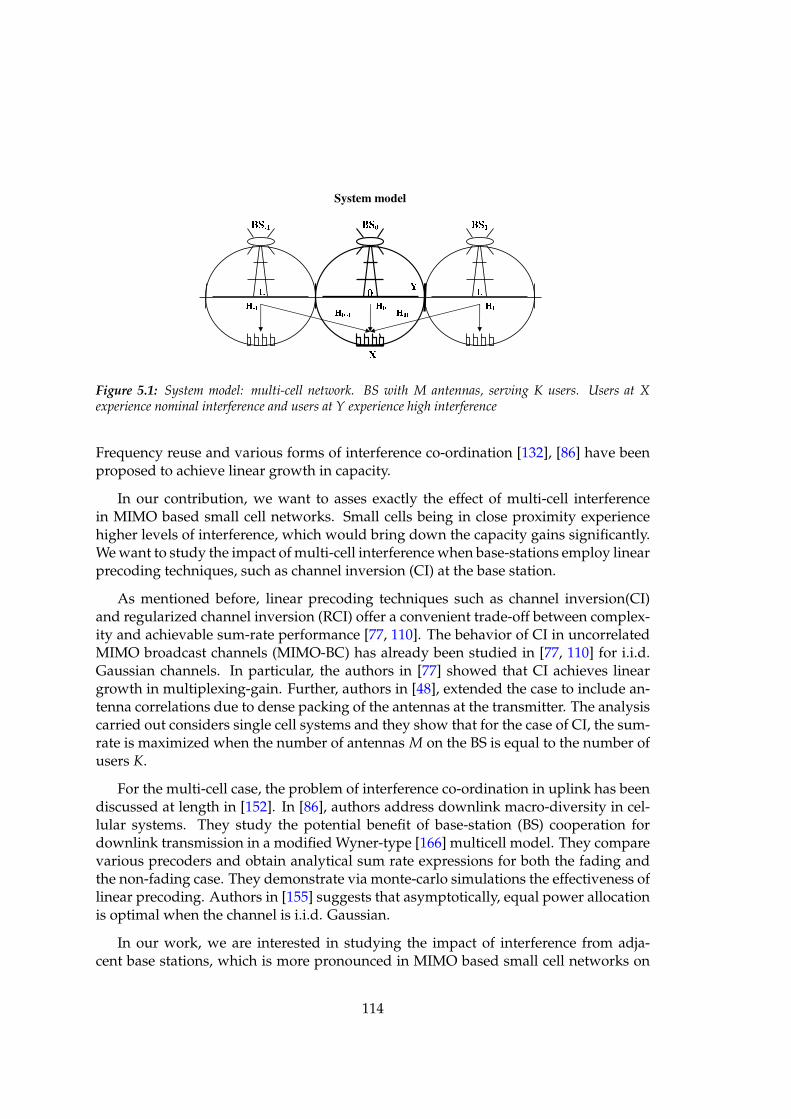
Figure 5.1: System model: multi-cell network. BS with M antennas, serving K users. Users at Xexperience nominal interference and users at Y experience high interference

Frequency reuse and various forms of interference co-ordination [132], [86] have beenproposed to achieve linear growth in capacity.

In our contribution, we want to asses exactly the effect of multi-cell interferencein MIMO based small cell networks. Small cells being in close proximity experiencehigher levels of interference, which would bring down the capacity gains significantly.We want to study the impact of multi-cell interference when base-stations employ linearprecoding techniques, such as channel inversion (CI) at the base station.

As mentioned before, linear precoding techniques such as channel inversion(CI)and regularized channel inversion (RCI) offer a convenient trade-off between complex-ity and achievable sum-rate performance [77, 110]. The behavior of CI in uncorrelatedMIMO broadcast channels (MIMO-BC) has already been studied in [77, 110] for i.i.d.Gaussian channels. In particular, the authors in [77] showed that CI achieves lineargrowth in multiplexing-gain. Further, authors in [48], extended the case to include an-tenna correlations due to dense packing of the antennas at the transmitter. The analysiscarried out considers single cell systems and they show that for the case of CI, the sum-rate is maximized when the number of antennas M on the BS is equal to the number ofusers K.

For the multi-cell case, the problem of interference co-ordination in uplink has beendiscussed at length in [152]. In [86], authors address downlink macro-diversity in cel-lular systems. They study the potential benefit of base-station (BS) cooperation fordownlink transmission in a modified Wyner-type [166] multicell model. They comparevarious precoders and obtain analytical sum rate expressions for both the fading andthe non-fading case. They demonstrate via monte-carlo simulations the effectiveness oflinear precoding. Authors in [155] suggests that asymptotically, equal power allocationis optimal when the channel is i.i.d. Gaussian.

In our work, we are interested in studying the impact of interference from adja-cent base stations, which is more pronounced in MIMO based small cell networks on

114

the achievable sum-rate capacity. We consider multiple-input multiple-output (MIMO)multi-cell systems, each cell composed of a transmitter equipped with M antennas andK single-antenna receivers. We consider Wyner-type cellular models in our study. Weneglect the effects of channel correlation due to densely packed antennas at the base-station transmitter, with a view to keep the analysis tractable.

The analytic expressions of the sum-rates for CI are derived by applying recent toolsfrom random matrix theory (RMT . These expressions are independent of the specificchannel realizations.

In our study, we find that

• The achievable sum-rate is significantly diminished by the effect of multi-cell in-terference in MIMO based small cell networks.

• The sum-rate capacity tends to grow sub-linearly with respect to the number ofbase-station antennas as long as the interference is non-zero.

• Also, there is an optimal number of users for a given number of antennas at thetransmitter, which maximizes the sum-capacity. This depends on the interferencelevel and the transmit power at the base-station.

The remainder of this chapter is organized as follows: Section 5.2 briefly reviewsvarious tools of random matrix theory which will be used in later derivations. Section5.3 introduces the multi-cell system model. In Section 5.4 we study channel inversionprecoding. Section 5.5 provides simulation results which are shown to corroborate thetheoretical derivations. Finally in Section 5.6 we provide our conclusions.

Notations: In the following, boldface lower-case symbols represent vectors, capitalboldface characters denote matrices (IN is the N × N identity matrix). The Hermitiantranspose is denoted (·)H. The operator tr[X] represents the trace of matrix X. Theeigenvalue distribution of an Hermitian random matrix X is µX(x). The symbol E[·]denotes expectation. The derivative of a function f (x) of a single variable x is denotedf ′(x). All logarithms are base-2 logarithms.

5.2 Random Matrix Theory Tools

In this work, we are interested in the behavior of large random Hermitian matrices,and particularly in the asymptotic distribution of their eigenvalues. Specifically, theeigenvalue distribution of large Hermitian matrices converges, in many practical cases,to a definite probability distribution, hereafter called the empirical distribution of therandom matrix, when the matrix dimensions grow to infinity.

A tool of particular interest in this work is the Stieltjes transform SX of a large Hermi-tian non-negative definite matrix X, defined on the half the space C

+ = C \ R+ = z ∈C, Re(z) < 0, as

SX(z) =∫ +∞

0

1λ − z

µX(λ)dλ (5.1)

115

where µX is the empirical distribution of X.

Couillet et al. [47] derived a fixed-point expression of the Stieltjes transform forGaussian matrices with correlations in the following theorem,Theorem 5.2.0.1. Let the entries of the K × M matrix W be i.i.d. Gaussian with zero meanand variance 1/M. Let X and Q be respectively K × K and M × M Hermitian non-negativedefinite matrices with eigenvalue distributions µX and µQ. We impose further that the largesteigenvalues of X and Q are bounded independently of K, M. Let Y be an K × K Hermitianmatrix with the same eigenvectors as X and let f be some function mapping the eigenvalues ofX to those of Y. Let z ∈ C

+ = C \ R+. Then, for M, K large with K/M = 1/β, the Stieltjes

transform SH(z) of H = X1/2WQWHX1/2 + Y is given

SH(z) =∫

(

f (x) + x∫ q · µQ(q)q.

1 + 1β qTH(z)

− z

)−1

µX(x)x. (5.2)

where TH is a solution of the fixed-point equation

TH(z) =∫

x

(

f (x) + x∫ q · µQ(q)q.

1 + 1β qTH(z)

− z

)−1

µX(x)x. (5.3)

An immediate corollary, when only right-correlation is considered, unfolds natu-rally as follows,Corollaire 5.2.1. [130] Let the entries of the K × M matrix W be i.i.d. Gaussian with zeromean and variance 1/M. Let Y be an K × K Hermitian non-negative matrix with eigenvaluedistribution µY(x). Moreover, let Q be a M × M non-negative definite matrix with eigenvaluedistribution µQ(x), such that the eigenvalues of Q are bounded irrespectively of M. Then, forlarge K, M, such that K/M = α, the Stieltjes transform on C

+ of the matrix

H = WQWH + Y (5.4)

verifies

SH(z) = SY

(

z −∫

q

1 + αqSH(z)µQ(q)dq

)

(5.5)

5.3 System model and assumptions

We discuss the system model in this section. We consider a multi-cell Wyner-typemodel, for example as shown in figure (5.1). For simplicity and to be able to keepthe analysis tractable, we consider a three-cell network. The cell at the center is our ref-erence. The users in this cell experience interference from the neighboring base stationsas shown. Each cell serves K users from a base-station with M antennas. We assumethat the base station antennas are uncorrelated. The information from the base-stationto its user set is precoded assuming perfect channel state information at the transmit-ter (CSIT). i.e, each base station knows perfectly the channel towards the users in its

116

cell, but not the interfering channels. Users receive desired signal plus interference sig-nals from adjacent base stations. We assume channel inversion (CI) precoding at thetransmitter. The transmitted signals from the base stations undergo Rayleigh fadingand path-loss. Further, we assume that the channel is constant for some interval longenough for the transmitter to learn and use it until it changes to a new value. We areinterested in the behavior of the system and its sum-rate capacity. Many of our resultsare obtained for large limits, because the limiting results are often tractable. Neverthe-less, we often consider M, K small in our simulation examples. Further, all users areassumed to have the same average (but not instantaneous) received signal power, soour model assumes that the users are similar distances from the base station and arenot in deep shadow fades.

5.4 Channel inversion precoding

Channel inversion precoding, also referred to as zero-forcing (ZF) precoding, annihi-lates all the inter-user interference by performing an inversion of the channel matrix Hat the transmitter. We begin our analysis with the single cell case, which is discussed indetail in [48], [77], and further we shall consider the multi-cell case.

5.4.1 Single cell

Without loss of generality, we consider cell 0. The signal received by users in this cell is

y = Hx + n. (5.6)

where, H is the K× M channel matrix with zero-mean unit-variance i.i.d complex Gaus-sian entries, x = Gs is the transmit vector obtained by linear precoding of the symbolvector s with the precoding matrix G. Symbol sk ∈ s for any user k is complex Gaussianwith zero mean and unit variance. The M × K linear precoding matrix is defined as

G = αHH

(

HHH

)−1. (5.7)

where α is chosen appropriately to satisfy the total transmit power constraint tr(E[xxH ]) ≤tr(GGH) ≤ P.

Now the received vector in Cell 0

y = αs + n. (5.8)

The parameter α which satisfies the transmit power constraint and depends only onthe channel realization H is given by

α2 =P

tr ((HHH)−1)(5.9)

117

The SNR (signal to noise ratio) for any user k is defined as

ηk =Es

[

|αsk|2]

E|nk|2=

α2

σ2 . (5.10)

is independent of the selected user. σ2 is the noise variance.

The ergodic capacity for user k is

Ck = log(1 + ηk). (5.11)

and the sum-rate is

Rci =K

∑k=1

log(1 + ηk). (5.12)

5.4.2 Asymptotic analysis for a single-cell

α is a function of H and as M, K → ∞, α tends to a constant. Thus the sum-rate can bewritten as

Rci = K log (1 + ηk) (5.13)

Let us denote H′ =1√M

H. It follows from (5.9) that When M is large with M/K =

β,

1M

tr(

H′H′H)−1

=1M

K

∑i=1

1λi

=K

M

(

1K

K

∑i=1

1λi

)

=K

M

∫ 1λ

(

1K

K

∑i=1

δ(λ − λi)

)

dλ

=1β

∫ 1λ

µKH′H′H(λ)dλ

=1βSH′H′H(0)

As a consequence, for large (K, M)

α2

σ2 → ρβ

SH′H′H(0), where ρ = P/σ2 (5.14)

and the sum-rate is

Rci = K log(

1 +ρβ

SH′H′H(0)

)

(5.15)

118

According to Corollary 5.2.1, SH′H′H(0) is the solution of1

SH′H′H(0) =

(

∫

λ

1 + λβSH′H′H(0)

µ(λ)dλ

)−1

=

(

∫

λ δ(λ − 1)1 + λ

βSH′H′H(0)

)−1

=

(

1 +SH′H′H(0)

β

)

(5.16)

Solving for SH′H′H(0) yields,

SH′H′H(0) =β

(β − 1)(5.17)

and the sum-rate is re-written as

Rci = K log (1 + ρ(β − 1)) for β ≥ 1 (5.18)

The rate-per-antenna is

Rci

M=

1β

log (1 + ρ(β − 1)) . (5.19)

As β → 1, Rci/M → 0, which implies that the sum rate of channel inversion doesnot increase linearly with M (or K)

5.4.3 Optimizer β∗ for the single cell

Following [77] we now look for a value β⋆ of the ratio M/K such that, for a fixed num-ber of transmit antennas M, the sum-rate Rci(β) is maximized. By differentiating eqn(5.19) with respect to β and setting the derivative to zero, β∗ is the solution of the im-plicit equation

ρβ∗ = (1 + ρ(β∗ − 1)) log (1 + ρ(β∗ − 1)) (5.20)

1it is important to note here that we slightly misapply Corollary 5.2.1 since the result is only provenvalid outside for any z > 0.

119

5.4.4 Multi-cell

In this section, we study the effect of multi-cell interference. Without loss of generality,we consider users in Cell 0 affected by interference from adjacent base-stations. Weconsider a 3-cell Wyner-type model as shown in figure 5.1. Cell C0 is at the center.Adjacent cells are designated Cell C1 and Cell C−1.

Following our analysis of the single cell case, the received vector for users of cell C0,is

y = H0G0s0 +√

γH01G1s1 +√

γH0−1G−1s−1 + n. (5.21)

As before, H0 is the channel matrix from base station in cell C0 to its users. H01 andH0−1 are interfering channels from cell C1 and C−1, respectively. G1 and G−1 are pre-coding matrices for users in cell C1 and C−1, respectively. γ is the signal (interference)attenuation.

As stated earlier, all users in cell C0 are assumed to have the same average receivedsignal power, so our model assumes that the users are similar distances from the basestation and are not in deep shadow fades.

The precoding matrices in cell i can be written as

Gi = αiHH

i (HiHH

i )−1 (5.22)

The ergodic capacity for user k in cell C0 is expressed as

Ck = log(

1 +α2

0

E[|nk|2]

)

(5.23)

Where, nk is the kth element of the covariance matrix n. The expectation of this matrixcan be written as

E[nnH] = γH01G1GH

1 HH

01

+ γH0−1G−1GH

−1HH

0−1 + σ2I (5.24)

Expanding and simplifying,

E[nnH] = γα21H01HH

1 (H1HH

1 )−2H1HH

01

+ γα2−1H0−1HH

−1(H−1HH

−1)−2H−1HH

0−1

+ σ2I (5.25)

Since,

E[|n1|2] = E[|n2|2] . . . = E[|nk|2] (5.26)

We can write,

E[|nk|2] → 1K

K

∑k=1

E[|ni|2]

=1K

tr(

E[nnH])

(5.27)

120

E[|nk|2] =1K

tr(

γα21H01HH

1 (H1HH

1 )−2H1HH

01

+ γα2−1H0−1HH

−1(H−1HH

−1)−2H−1HH

0−1

)

+σ2I (5.28)

5.4.5 Asymptotic analysis for the multi-cell

Lemma 5.4.6. As K, M → ∞

1K

tr(

H01HH

1 (H1HH

1 )−2H1HH

01

)

→ 1β − 1

Proof: DenoteA = HH

1 (H1HH

1 )−2H1

Now,

1K

tr(

H01AHH

01

)

=1K

E[

tr(

H01AHH

01

)]

=1K

tr(

E[

H01AHH

01

])

=1K

tr (E [tr(A)] IK×K)

= E [tr(A)]

= E[

tr(

HH

1 (H1HH

1 )−2H1

)]

= E[

tr(

H1HH

1 )−1)]

If K × M matrix H1 is zero-mean, i.i.d. Gaussian, then W = H1HH

1 is a Wishart matrix.For a Wishart matrix 2,

E[

tr(

W)−1)]

=K

M − K

E[

tr(

H1HH

1 )−1)]

=K

M − K=

1β − 1

and hence,

1K

tr(

H01HH

1 (H1HH

1 )−2H1HH

01

)

→ 1β − 1

2Refer section 2.1.6, equation (2.9) of [149] and the references there-in ([71, 97])

121

Thus the expectation in eq. (5.28) reduces to,

E[|nk|2] → α21γ

1β − 1

+ α2−1γ

1β − 1

+ σ2 (5.29)

And hence, the sum-rate is

Rci = K log

(

1 +α2

0(β − 1)α2

1γ + α2−1γ + σ2(β − 1)

)

(5.30)

Following (5.14), for large (K, M),

α20

σ2 =α2

1σ2 =

α2−1

σ2 → ρβ

SH′H′H(0), where ρ = P/σ2 (5.31)

Thus the above sum-rate expression can be simplified as

Rci = K log(

1 +ρβ(β − 1)

(β − 1)SH′H′H(0) + 2γρβ

)

(5.32)

Substituting for SH′H′H(0),

Rci = K log(

1 +ρ(β − 1)1 + 2γρ

)

(5.33)

Re-writing,

Rci

M=

1β

log(

1 +ρ(β − 1)1 + 2γρ

)

(5.34)

We observe that when γ = 0, that is when there is no interference, the capacity formulais that of the single-cell case.

As β → 1, Rci/M → 0, which implies that the sum rate of channel inversion doesnot increase linearly with M (or K)

5.4.7 Optimizer β∗ for the multi-cell

Following on similar lines of the single-cell case, we now look for a value β⋆ of theratio M/K such that, for a fixed number of transmit antennas M, the sum-rate Rci(β)is maximized. By differentiating eqn (5.34) with respect to β and setting the derivativeto zero, β∗ is the solution of the implicit equation

ρβ∗ = [ρ(β∗ − 1) + (1 + 2γρ)] log[

1 +ρ(β∗ − 1)1 + 2γρ

]

(5.35)

One can observe that by setting γ = 0, we fall back to the implicit equation (5.20) of thesingle cell case.

122

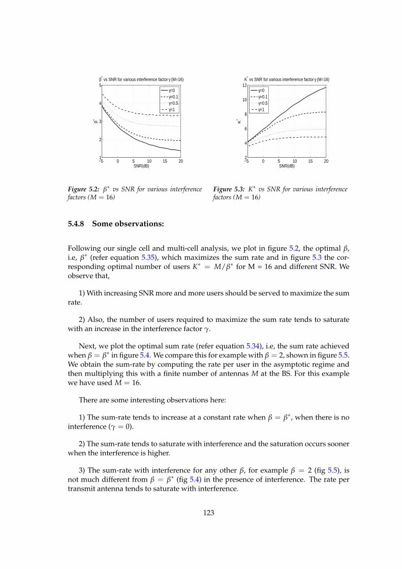
−5 0 5 10 15 201

2

3

4

5β* vs SNR for various interference factor γ (M=16)

SNR(dB)

β*

γ=0γ=0.1γ=0.5γ=1

Figure 5.2: β∗ vs SNR for various interferencefactors (M = 16)

−5 0 5 10 15 202

4

6

8

10

12K* vs SNR for various interference factor γ (M=16)

SNR(dB)

K*

γ=0γ=0.1γ=0.5γ=1

Figure 5.3: K∗ vs SNR for various interferencefactors (M = 16)

5.4.8 Some observations:

Following our single cell and multi-cell analysis, we plot in figure 5.2, the optimal β,i.e, β∗ (refer equation 5.35), which maximizes the sum rate and in figure 5.3 the cor-responding optimal number of users K∗ = M/β∗ for M = 16 and different SNR. Weobserve that,

1) With increasing SNR more and more users should be served to maximize the sumrate.

2) Also, the number of users required to maximize the sum rate tends to saturatewith an increase in the interference factor γ.

Next, we plot the optimal sum rate (refer equation 5.34), i.e, the sum rate achievedwhen β = β∗ in figure 5.4. We compare this for example with β = 2, shown in figure 5.5.We obtain the sum-rate by computing the rate per user in the asymptotic regime andthen multiplying this with a finite number of antennas M at the BS. For this examplewe have used M = 16.

There are some interesting observations here:

1) The sum-rate tends to increase at a constant rate when β = β∗, when there is nointerference (γ = 0).

2) The sum-rate tends to saturate with interference and the saturation occurs soonerwhen the interference is higher.

3) The sum-rate with interference for any other β, for example β = 2 (fig 5.5), isnot much different from β = β∗ (fig 5.4) in the presence of interference. The rate pertransmit antenna tends to saturate with interference.

123

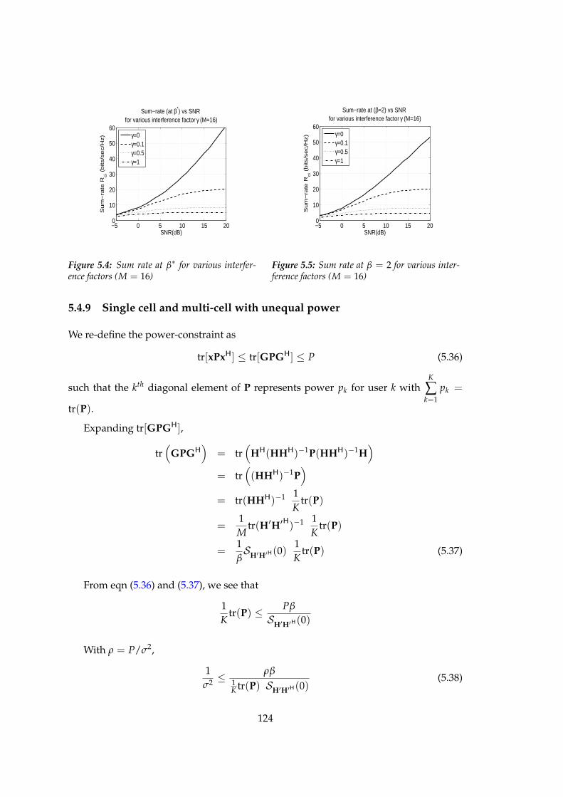
−5 0 5 10 15 200

10

20

30

40

50

60

Sum−rate (at β*) vs SNR for various interference factor γ (M=16)

SNR(dB)

Su

m−

rate

Rci (

bits/s

ec/H

z) γ=0

γ=0.1γ=0.5γ=1

Figure 5.4: Sum rate at β∗ for various interfer-ence factors (M = 16)

−5 0 5 10 15 200

10

20

30

40

50

60

SNR(dB)

Su

m−

rate

Rci (

bits/s

ec/H

z)

Sum−rate at (β=2) vs SNR for various interference factor γ (M=16)

γ=0γ=0.1γ=0.5γ=1

Figure 5.5: Sum rate at β = 2 for various inter-ference factors (M = 16)

5.4.9 Single cell and multi-cell with unequal power

We re-define the power-constraint as

tr[xPxH] ≤ tr[GPGH] ≤ P (5.36)

such that the kth diagonal element of P represents power pk for user k withK

∑k=1

pk =

tr(P).

Expanding tr[GPGH],

tr(

GPGH

)

= tr(

HH(HHH)−1P(HHH)−1H)

= tr(

(HHH)−1P)

= tr(HHH)−1 1K

tr(P)

=1M

tr(H′H′H)−1 1K

tr(P)

=1βSH′H′H(0)

1K

tr(P) (5.37)

From eqn (5.36) and (5.37), we see that

1K

tr(P) ≤ Pβ

SH′H′H(0)

With ρ = P/σ2,

1σ2 ≤ ρβ

1K tr(P) SH′H′H(0)

(5.38)

124

Substituting SH′H′H(0) = β/(β − 1), the ergodic capacity for user k in the single-cellcase is

Ck = log(

1 +pk

σ2

)

= log

(

1 +pkρ(β − 1)

1K tr(P)

)

. (5.39)

and the sum-rate is

Rci =K

∑k=1

log

(

1 +pkρ(β − 1)

1K tr(P)

)

. (5.40)

We can easily see that with equal power for all users,1K

tr(P) = p = pk and the above

expression will reduce to the expressions derived for the single-cell case with equalpower constraint (eqn 5.18).

The rate per antenna is

Rci

M=

1β

1K

K

∑k=1

log

(

1 +pkρ(β − 1)

1K tr(P)

)

(5.41)

For the multi-cell case, the ergodic capacity eqn (5.23) for user k is

Ck = log(

1 +pk

E[|nk|2]

)

(5.42)

Where,

E[nnH] = γH01G1P1GH

1 HH

01

+ γH0−1G−1P−1GH

−1HH

0−1

+ σ2I (5.43)

After suitable simplification similar to the multi-cell analysis in the previous section,we can re-write the above expression as

E[|nk|2] =1K

tr(

H01HH

1 (H1HH

1 )−1

P1(H1HH

1 )−1

H1HH

01

+H0−1HH

−1(H−1HH

−1)−1

P−1(H−1HH

−1)−1

H−1HH

0−1

)

+σ2I (5.44)

As M, K → ∞,

tr(

H01HH

1 (H1HH

1 )−1Pi(H1HH

1 )−1H1HH

01

)

→ 1β − 1

tr(Pi) (5.45)

125

Therefore, the expectation can be written as,

E[|nk|2] = γ1

β − 1tr(P1)

K+ γ

1β − 1

tr(P−1)

K

+σ2I. (5.46)

The capacity of user k is

Ck = log

(

1 +(β − 1) pk

γ tr(P1)K + γ tr(P−1)

K + σ2(β − 1)

)

(5.47)

Substituting eqn (5.38) for 1/σ2,

Ck = log

(

1 +ρ(β − 1) pk

γρ tr(P1)K + γρ tr(P−1)

K + tr(P)K

)

(5.48)

and the sum-rate is expressed as

Rci =K

∑k=1

log

(

1 +ρ(β − 1) pk


K + tr(P)K

)

(5.49)

Notice that if1K

tr(Pi) = p = pk, the above expression will reduce to the expressions

derived for the multi-cell case with equal power constraint (eqn 5.33).

The sum-rate per antenna is

Rci

M=

1β

1K

K

∑k=1

log

(

1 +ρ(β − 1) pk


K + tr(P)K

)

(5.50)

We observe two things here. 1) One can come up with an optimal power allocationpolicy (for ex. based on the channel characteristics) which maximizes the sum-capacityin the unequal power allocation scheme. 2) If some of the users in the adjacent base sta-tions are not being serviced, i.e, their respective antenna at the transmitter is switchedoff, the interference comes down (for ex. if one or more user links are inactive in cell 1,then tr(P1) < P1) and hence the sum-capacity scales up.

5.5 Simulation results

In this section we evaluate by simulation how interference from neighboring base sta-tions impacts the behavior of the sum-rate of linearly precoded MIMO small cell net-works when the antenna array at the transmitter are large. We compare numerical

126

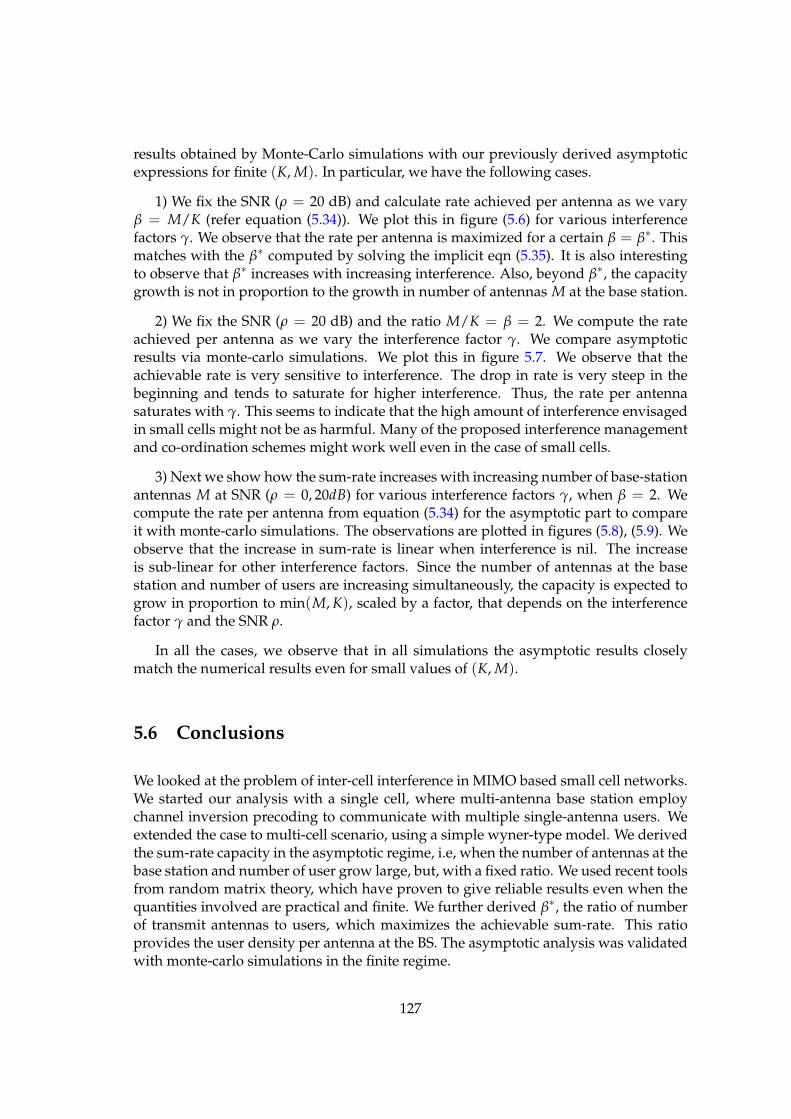
results obtained by Monte-Carlo simulations with our previously derived asymptoticexpressions for finite (K, M). In particular, we have the following cases.

1) We fix the SNR (ρ = 20 dB) and calculate rate achieved per antenna as we varyβ = M/K (refer equation (5.34)). We plot this in figure (5.6) for various interferencefactors γ. We observe that the rate per antenna is maximized for a certain β = β∗. Thismatches with the β∗ computed by solving the implicit eqn (5.35). It is also interestingto observe that β∗ increases with increasing interference. Also, beyond β∗, the capacitygrowth is not in proportion to the growth in number of antennas M at the base station.

2) We fix the SNR (ρ = 20 dB) and the ratio M/K = β = 2. We compute the rateachieved per antenna as we vary the interference factor γ. We compare asymptoticresults via monte-carlo simulations. We plot this in figure 5.7. We observe that theachievable rate is very sensitive to interference. The drop in rate is very steep in thebeginning and tends to saturate for higher interference. Thus, the rate per antennasaturates with γ. This seems to indicate that the high amount of interference envisagedin small cells might not be as harmful. Many of the proposed interference managementand co-ordination schemes might work well even in the case of small cells.

3) Next we show how the sum-rate increases with increasing number of base-stationantennas M at SNR (ρ = 0, 20dB) for various interference factors γ, when β = 2. Wecompute the rate per antenna from equation (5.34) for the asymptotic part to compareit with monte-carlo simulations. The observations are plotted in figures (5.8), (5.9). Weobserve that the increase in sum-rate is linear when interference is nil. The increaseis sub-linear for other interference factors. Since the number of antennas at the basestation and number of users are increasing simultaneously, the capacity is expected togrow in proportion to min(M, K), scaled by a factor, that depends on the interferencefactor γ and the SNR ρ.

In all the cases, we observe that in all simulations the asymptotic results closelymatch the numerical results even for small values of (K, M).

5.6 Conclusions

We looked at the problem of inter-cell interference in MIMO based small cell networks.We started our analysis with a single cell, where multi-antenna base station employchannel inversion precoding to communicate with multiple single-antenna users. Weextended the case to multi-cell scenario, using a simple wyner-type model. We derivedthe sum-rate capacity in the asymptotic regime, i.e, when the number of antennas at thebase station and number of user grow large, but, with a fixed ratio. We used recent toolsfrom random matrix theory, which have proven to give reliable results even when thequantities involved are practical and finite. We further derived β∗, the ratio of numberof transmit antennas to users, which maximizes the achievable sum-rate. This ratioprovides the user density per antenna at the BS. The asymptotic analysis was validatedwith monte-carlo simulations in the finite regime.

127

1 2 3 4 5 60

1

2

3

4Rate per antenna vs β (SNR=20dB)

β

Rate

per

ante

nna (

bits/s

ec/H

z) γ=0

γ=0.1γ=0.5γ=1

Figure 5.6: Rate per antenna vs β at SNR of 20dB for various interference factors γ

0 0.2 0.4 0.6 0.8 10

0.5

1

1.5

2

2.5

3

3.5Rate per antenna vs γ (SNR=20dB)

γ

Rate

per

ante

nna (

bits/s

ec/H

z)

sim

asy

Figure 5.7: Rate per antenna vs γ, when, β = 2,SNR ρ = 20 dB for various interference factors γ

5 10 15 20 25 300

2

4

6

8

10

12

14

16Sum−rate vs M (SNR=0dB)

M

su

m−

rate

Rci (

bits/s

ec/H

z)

γ=0

γ=0.1

γ=0.5

γ=1

Figure 5.8: Sum rate per antenna as a function ofM for β = 2 at SNR of 0 dB for various interfer-ence factors

5 10 15 20 25 300

20

40

60

80

100

120Sum−rate vs M (SNR=20dB)

M

su

m−

rate

Rci (

bits/s

ec/H

z)

γ=0

γ=0.1

γ=0.5

γ=1

Figure 5.9: Sum rate per antenna as a function ofM for β = 2 at SNR of 20 dB for various inter-ference factors

128

We conclude that the achievable sum-rate is significantly diminished by the effect ofmulti-cell interference in MIMO based small cell networks. The sum-rate capacity tendsto grow sub-linearly with increasing interference. Also, there is an optimal number ofusers for a given number of antennas at the transmitter, which maximizes the sum-capacity. This depends on the interference level and the transmit power at the base-station. For a given number of transmit antenna, moving away from the optimal, β∗,tends to saturate the capacity growth at high SNR. The saturation occurs sooner withhigher interference.

5.7 Publications

1. Sreenath Ramanath, Merouane Debbah, Eitan Altman, Vinod Kumar, "Asymp-totic analysis of precoded small cell networks", proceedings of InfoCom 2010, Mar15-19, San Diego, USA.

129

Chapter 6

Open Loop Control of BSDeactivation


6.2 Multimodularity . . . . . . . . . . . . . . . . . . . . . . . . . . . . . . . 133

6.3 Centralized optimal control . . . . . . . . . . . . . . . . . . . . . . . . . 134

6.4 Decentralized optimal control . . . . . . . . . . . . . . . . . . . . . . . 136

6.5 Future Directions . . . . . . . . . . . . . . . . . . . . . . . . . . . . . . . 137

6.6 Conclusions . . . . . . . . . . . . . . . . . . . . . . . . . . . . . . . . . . 138

6.7 Publications . . . . . . . . . . . . . . . . . . . . . . . . . . . . . . . . . . 141

6.1 Introduction

In recent years, there is a paradigm shift towards greener and denser networks [39,81]. While green networks aim at reducing overall power and energy consumption innetworks, denser networks increase the capacity and coverage of networks. Typically,dense networks, popularly referred to as small cell networks comprise Femto and picocells serving indoor, hot-spot and urban mobility regions. The base stations used insuch cells are compact and small portable devices, which can be easily installed onexisting infrastructure and are often battery operated. They recharge periodically and itwould be beneficial from a greener perspective if this can be as less frequent as possible.Thus these base stations need to judiciously use the available battery power. Further,if one assumes that all these base stations are accessible to a central control unit via aback haul link, depending on the load, some of these devices can be switched OFF toconserve their battery life.

In our current work, we derive optimal policies to conserve energy in two scenarios.1) A central control unit, which, depending on the load in the system can switch OFF

131

certain base stations to reduce overall energy conservation in the system, but, withan objective to maximize the expected throughput. 2) Each base station can derive itspolicy independent of its neighbors to minimize an average cost metric (for example,its buffer occupancy), while keeping a lower bound on the fraction of time the it isswitched OFF. To address these problems, we use tools from Multimodularity.

The natural counterpart of convex functions over integer sets turn out to be the socalled Multimodular functions ([75]) and for such functions we have indeed the propertythat local minima are global minima. The property of Multimodularity can handle thecontrol of discrete events and we utilize the same to obtain optimal activation policiesfor base stations. These tools were earlier used in the context of stochastic control ofQueuing systems ([12] and reference therein). In a recent work [34], while addressingthe problem of energy limited wireless handsets, the authors use tools from Multimod-ularity to address open loop control and establish optimality of bracket sequences basedcontrol.

We consider a regular network, wherein the base stations form a linear network andhere the tools of Multimodularity fit in. Tools like stochastic geometry can be used toaddress networks which have base stations and mobiles distributed stochastically ac-cording to some given process (for eg. Poisson) and this study is not addressed here.Our objective is to obtain open loop policies. Later, we plan to derive closed loop poli-cies for the same. The main results from this chapter are:

1. We show that the cost structure for the both centralized and decentralized scenar-ios is Multimodular.

2. For the central control, among all feasible policies with at least an asymptoticfraction ρ of the base stations being switched OFF, the bracket policy with rate ρis optimal.

3. For the decentralized control, among all feasible policies with the BS switchedOFF for at least an asymptotic fraction ρ of the time, the bracket policy with rateρ is optimal.

4. In both the cases, the optimal policy is given by (⌊x⌋ denotes the largest integersmaller or equal to x)

an = ⌊nρ⌋ − ⌊(n − 1)ρ⌋.

Here, an = 0(1), if the n-th BS (centralized) or BS in the n-th time slot (decentral-ized) is switched OFF (ON).

5. The optimal policies depend only upon the conservation factor ρ and are inde-pendent of all other system parameters, for example path loss coefficient, powerper transmission, etc.

In both the problems, we call ρ, the switch OFF fraction (the total fraction of basestations to be switched OFF in central control or the fraction of time a base station isswitched OFF in decentralized control), as the conservation factor. In the first case, thisis decided by the central control based on system statistics (like traffic type, load distri-bution, QoS, time of hour, day of week, power saving, etc.), while in the decentralized

132

case, it is derived based on resources available and the QoS setting (memory, powersaving, waiting time, sojourn time, etc.). Further, in our analysis, we assume that thisfactor is known a priori.

Organization of the chapter: In Section 6.2, we introduce Multimodularity conceptsand the tools relevant in this work. In Section 6.3, we address the central control prob-lem, while Section 6.4 studies the decentralized control. In Section 6.5, we discuss somepossible future directions and we conclude our work in Section 6.6.

Notations: Bold letters, for example a, represent an infinite sequence while akj rep-

resents a part of this sequence defined by (aj, · · · , ak). Let 1n1 represent a n vector of all

ones while 1 represents the infinite sequence of all ones. In the sections, where the infi-nite sequences are not used and where all the vectors used are of the same length, thenbold letters (for example a) themselves are used to represent the finite length vectors.lim, lim is limit infimum and supremum, respectively.

6.2 Multimodularity

Multimodularity can be used to address a wide class of control problems over se-quences of integer numbers. Multimodular functions turn out to be the natural counterpart of Convex functions, in the case of integer valued functions, for which the existenceof a local minima guarantees a global minima. Also, they induce a particular form ofoptimal policies, which turn out to be very regular, and are described by the well knownbracket sequences. We reproduce the related definitions (see [12] for general definitions)specific to the spaces considered in this work.

In this section, we use notation a to represent the N−length vector aN1 as here we do

not need the infinite length sequences.Definition 6.2.0.1. A function f : 0, 1N → R is Multimodular if

f (a + v) + f (a + u) ≥ f (a) + f (a + u + v) (6.1)

for all a ∈ 0, 1N and for all u, v ∈ F with u 6= v and such that a + u, a + v, a + u + v ∈0, 1N .

The Multimodular base F contains the vectors −e1, s2, s3, · · · , sN , eN, where,

−e1 = (−1 0 0 0 0 . . . 0 0),s2 = (1 − 1 0 0 0 . . . 0 0),s3 = (0 1 − 1 0 0 . . . 0 0),· · · ,sN = (0 0 0 0 0 . . . 1 − 1) andeN = (0 0 0 0 0 . . . 0 1)

Definition 6.2.0.2. The bracket sequence a(ρ, θ) := an(ρ, θ) with rate ρ ∈ [0, 1) and initialphase θ ∈ [0, 1) is defined as

an(ρ, θ) = ⌊nρ + θ⌋ − ⌊(n − 1)ρ + θ⌋ (6.2)

133

In this work, we mainly use Theorem 6, pp. 25, [12] which establishes the optimalityof bracket sequences and the same is reproduced here.Theorem 6.2.0.3. A bracket sequence a(ρ, θ) for any θ ∈ [0, 1) minimizes the cost

limN→∞

1N

N

∑n=1

fn(a1, · · · , an)

over all the sequences that satisfy

limN→∞

1N

N

∑n=1

an ≥ ρ,

when ρ ∈ [0, 1), under the following assumptions:

A.1 fn is Multimodular ∀n.

A.2 fn(a1, . . . , an) ≥ fn−1(a2, . . . , an), ∀n > 1 and

A.3 for any sequence an, ∃ a sequence bn such that ∀n, m with n > m,

fn(b1, . . . , bn−m, a1, . . . , am) = fm(a1, . . . , am)

A.4 all functions fn(a1, · · · , an) are increasing in all ai.

6.3 Centralized optimal control

We have uniformly placed points on a line, which are separated by a distance d. Eachpoint can potentially contain a BS and / or a mobile. The mobile at any point is active(i.e., has a communication request) with probability q and this process is identical andindependent across the space. Some of the base stations are switched OFF to optimizethe battery performance. Every BS that is ON is associated to some of the mobiles basedon the nearest distance criterion. Further the BS uses directional antennae and can onlycommunicate with the users to its right. The throughput at the base station from amobile located at distance r is given by

θ = q log(

1 +pr−β

σ2

)

,

where p, r, β, σ2 respectively represent the transmit power from mobile, distance be-tween BS and mobile, path loss factor and the noise variance. Further we assume thatthere is no intra or inter-cell interference. Note that the throughput is achieved onlywhen the mobile has a request, which occurs with probability q.

Our goal is to find an optimal switch OFF pattern of the base stations so as to maximize thesum of the expected throughputs of all the mobiles when one has to at least switch OFF a fractionρ of the base stations. The conservation factor ρ at any time period will be decided by the

134

network based on the load and for a given ρ the network prefers to adopt an optimalON-OFF pattern.

We obtain this answer in the asymptotic as N, the number of points in the space tendto ∞. Consider a sequence a ∈ 0, 1∞ to represent the control sequence in the follow-ing sense: ai, the action at ith point is 1 if BS is switched OFF and 0 if BS is ON. The goalis to find an optimal sequence a∗ which maximizes the expected throughput (definedvia Cesaro limit) such that the total fraction of the base stations, that are switched OFF,is lower bounded by ρ. We assume that the system starts at point 0 where a BS is alwaysswitched ON and we control the ON-OFF status of the remaining base stations, i.e., theones starting from point 1 onwards. We neglect the throughput due to the mobile at 0as it does not contribute to optimization. Thus, we maximize

maxa

limN→∞

1N

N

∑n=1

θn(a) (6.3)

subject to limN→∞

1N

N

∑n=1

an ≥ ρ (6.4)

where θn(a) is the throughput due to the mobile at position n (which depends uponthe position of the nearest base station). This depends upon the sequence a and equals(note the base station at point 0 is always ON):

θn(a) = q log

(

1 +p(

1 + r2n

)−β/2

σ2

)

where (6.5)

rn :=

nd if an1 = 1n

1inf

1≤j≤n

|n − j|d : aj = 0

else. (6.6)

We use tools from Multimodularity [12] to address this problem. The related defi-nitions are summarized in section 6.2. We use Theorem 6.2.0.3 and obtain (proof is inAppendix A)Theorem 6.3.0.4. The function fn(an

1) := −θn(a) is Multimodular for every n. Further, thecentralized problem (6.3) is optimized by a bracket sequence (6.2),

a∗ = a(ρ, θ) for some θ ∈ [0, 1). ⋄

From the above theorem it is clear that the optimal sequence depends only uponthe conservation factor ρ and nothing else. We now give some examples of bracket se-quences. Example 1: The bracket sequence 100100100 maximizes the expected through-put for (ρ, θ) = (0.33, 0.9) . Example 2: The bracket sequence 1001001000 maximizes theexpected throughput for (ρ, θ) = (0.3, 0.9) . If the factor ρ is rational, then the sequenceis periodic ([75]). In this case the optimal policy is to switch OFF the base stations in aperiodic fashion, for example with ρ = 0.33 one needs to switch OFF every third BS.The optimality of bracket sequence is established in the limit N, the number of points,tending to infinity. This would imply the bracket sequence would be nearly optimal for

135

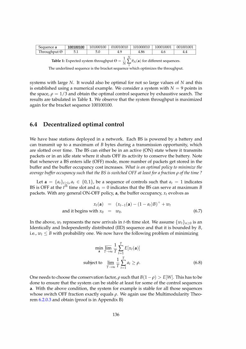
Sequence a 100100100 101000100 010010010 101000010 100010001 001001001Throughput Θ 5.1 5.0 4.9 4.86 4.6 4.4

Table 1: Expected system throughput Θ =1N

N

∑1

θN(a) for different sequences.

The underlined sequence is the bracket sequence which optimizes the throughput.

systems with large N. It would also be optimal for not so large values of N and thisis established using a numerical example. We consider a system with N = 9 points inthe space, ρ = 1/3 and obtain the optimal control sequence by exhaustive search. Theresults are tabulated in Table 1. We observe that the system throughput is maximizedagain for the bracket sequence 100100100.

6.4 Decentralized optimal control

We have base stations deployed in a network. Each BS is powered by a battery andcan transmit up to a maximum of B bytes during a transmission opportunity, whichare slotted over time. The BS can either be in an active (ON) state where it transmitspackets or in an idle state where it shuts OFF its activity to conserve the battery. Notethat whenever a BS enters idle (OFF) mode, more number of packets get stored in thebuffer and the buffer occupancy cost increases. What is an optimal policy to minimize theaverage buffer occupancy such that the BS is switched OFF at least for a fraction ρ of the time ?

Let a = att≥1, at ∈ 0, 1, be a sequence of controls such that at = 1 indicatesBS is OFF at the tth time slot and at = 0 indicates that the BS can serve at maximum Bpackets. With any general ON-OFF policy, a, the buffer occupancy, xt evolves as

xt(a) = (xt−1(a)− (1 − at)B)+ + wt

and it begins with x0 = w0. (6.7)

In the above, wt represents the new arrivals in t-th time slot. We assume wtn≥0 is anIdentically and Independently distributed (IID) sequence and that it is bounded by B,i.e., wt ≤ B with probability one. We now have the following problem of minimizing

mina

limT→∞

1T

T

∑t=1

E[xt(a)]

subject to limT→∞

1T

T

∑t=1

at ≥ ρ. (6.8)

One needs to choose the conservation factor, ρ such that B(1− ρ) > E[W]. This has to bedone to ensure that the system can be stable at least for some of the control sequencesa. With the above condition, the system for example is stable for all those sequenceswhose switch OFF fraction exactly equals ρ. We again use the Multimodularity Theo-rem 6.2.0.3 and obtain (proof is in Appendix B)

136

Theorem 6.4.0.5. The function ft(at1) := E[xt(a)] = E[xt(at

1)] is Multimodular for every t.And, the decentralized problem (6.8) is optimized by a bracket sequence.

a∗ = a(ρ, θ) for some θ ∈ [0, 1). ⋄

Thus the optimal sequence is again a bracket sequence which depends only on ρ,the conversation factor. Hence, in both centralized and decentralized problems, wehave similar optimal control pattern which in both the cases depends only upon theconservation factor ρ and none of the other design parameters.

6.5 Future Directions

We saw in previous examples how individual BS can decide switch OFF (in time) ora central control can switch OFF base stations (in space) to conserve the energy. Infuture, one can consider some more interesting problems which can be solved usingMultimodularity tools.

Optimization in space and time: We have uniformly placed M points on a line, whichare separated by a distance d. Each point can potentially contain a BS and a queue ofwaiting mobiles. We assume that the BS service is directional and they can potentiallyserve up to a maximum of B mobiles to the right in every time slot. The service orderof the mobiles depend on their proximity to the BS (to its left). Further, to conservepower, a central control can decide to switch OFF certain number of BS every timeslot. This scenario results from a network equipped with cooperative base stationsand in this case one needs to design an ON-OFF control that not only spans across thespace but also across time. We expect to obtain again a bracket sequence as the optimalsequence and now we further expect this sequence to have ’periodicity’ along space(when confined to the same time slot), have a small phase change in the next time slotand the periodicity in space continues.

Coverage problems: A mobile is covered, i.e., serviced when it is within a distance ndfrom a BS that is ON. One can study the optimal ON-OFF pattern which optimizes thefraction of the mobiles covered.

Closed Loop Policies: For the decentralized problem we would like to obtain theclosed loop policies. That is, we obtain the optimal policies, which at any time t de-pend upon the history up to time t − 1, (a∗t−1

1 , xt−11 ). We here consider minimizing the

finite time horizon problem

minaT

1 ∈AT

T

∑t=1

E[

xt(aT1 )− λat

]

where,

AT := aT1 ; for every t ≤ T, at : (at−1

1 , wt−11 ) 7→ 0, 1,

that is for every t the action at time t, at is a function of the history (at−11 , wt−1

1 ).

137

One can again use the tools of Multimodularity to obtain the structure of close loopoptimal policy. We propose to use Theorem 64, page 214, [12] to show that the optimalpolicy is a threshold policy in the following sense: for any given t and history a∗t−1

1 , xt−11

(optimal actions and optimal state trajectory till time t − 1), the optimal action at timet, a∗t is 0 until the state xt is above a threshold and is 1 otherwise.

6.6 Conclusions

In this chapter, we derived energy conserving policies for Base stations in regular greennetworks using tools from Multimodularity. We considered two example scenarios andshow how the cost functions are Multimodular. In the first case, for the case of cen-tral control, we derived the optimal open loop policies so as to maximize the expectedthroughput of the system given that at least a certain percentage of Base stations areswitched OFF. In the second case, we derived optimal open loop polices, which eachbase station can employ in a decentralized manner to minimize buffer occupancy costs,while keeping the long term average fraction of the BS switch OFF time at least abovea given threshold. We established the optimality of bracket policies for both the cases.We established that these regular sequences optimize the (respective) performance(s)and these sequences depend only upon the conservation factor and nothing else. Weconclude that Multimodularity can be applied in several interesting example scenariosto derive optimal control in Green Networks and provide some examples for futuredirection of research in this area.

Appendix A: Proofs related to centralized control

Proof of Theorem 6.3.0.4: The proof is obtained using Theorem 6.2.0.3 of section 6.2.By Theorem 6.6.0.6, the function fn(a1, · · · , an) = −θn(a) is Multimodular and henceassumption A.1 of Theorem 6.2.0.3 is satisfied.

Given an1 , define a0 = 0 and then define nb := arg inf

0≤j≤n|n − j| : aj = 0, to denote

the index of the nearest base station in the left for the mobile at point n. When nb > 1,assumption A.2 is satisfied as then fn(an

1) = fn−1(an2) = f (an

nb). When nb = 1 (i.e., when

an1 = (0, 1, · · · , 1)) the equality still holds in A.2 by the definition (6.5) of θn(a). When

an1 = 1n

1 , then the assumption A.2 is satisfied with inequality as θn(1n1) < θn−1(1n−1

1 ).

Assumption A.3 is satisfied by taking bn to be all zeros and clearly fn satisfies A.4.Thus all the hypothesis of Theorem 6.2.0.3 are satisfied and hence the theorem follows.⋄Theorem 6.6.0.6. For every n, fn is Multimodular.

Proof: All the sequences in this proof are n length vectors and hence we use the shortnotation a in place of an

1 . Consider any sequence a. We need to show for u 6= v ∈ F

138

(see section 6.2 for definitions) fn satisfies

fn(a + u) + fn(a + v) ≥ fn(a) + fn(a + u + v)

whenever, a + u, a + v, a + u + v are all in 0, 1n.

Without loss of generality let v = sj (see section 6.2) which result in shifting an ONposition of the base station from j − 1 location to location j. Since we can only considersuch sj for which a + sj is in 0, 1n the sequence a should have aj−1 = 0 and aj = 1.Further, (a + v)j−1 = 1 and (a + v)j = 0 while for every i 6= j or i 6= j − 1, ai = (a + v)i.Thus, addition of vector v to a results in changes in the base station associations andhence the throughputs, only for the the mobiles located in (j − 1, · · · , ηr

j − 1), where ηrj

is defined as the nearest base station to the right of the location j that is switched ON ina:

ηrj :=

arg infn>j

|n − k| : ak = 0 if set is non empty

n + 1 else.(6.9)

Hence,

fn(a)− fn(a + v) =n

∑k=1

θk(a)−n

∑k=1

θk(a + v)

=

ηrj −1

∑k=j−1

θk(a)− θk(a + v).

Let u = sl with l > j + 1 (l 6= j + 1 as then it is not possible that both a + u and a + vare in 0, 1n). The addition of u to a will introduce changes in mobile throughputsonly at locations (l − 1, · · · , ηr

l ), which do not overlap with locations changed by v,(j − 1, · · · , ηr

j ). Further, the addition of v to a + u also changes the mobile throughputsonly in locations (j − 1, · · · , ηr

j ) (w.r.t. the mobile throughputs under a + u). Becauseof the independence of the locations of the changes due to v and u and because themobile throughputs only depend upon the distance w.r.t. the serving BS, the mobilethroughput changes from a + u to a + u + v will be same as that when a is changed toa + v. Thus,

fn(a + u) − fn(a + u + v) =ηr

j

∑k=j−1

θk(a + u)− θk(a + u + v) =

ηrj

∑k=j−1

θk(a)− θk(a + v) =

fn(a)− fn(a + v). (6.10)

The second vector u can either be sl with l > j + 1 or l < j − 1 (as both a + u anda + v have to be in 0, 1n) or u can be en when j < n or it can e1 when j > 1. Inall the combinations, addition of vectors u and v results in changes to the base stationassociation at independent locations as above. Thus for any u 6= v, as in (6.10), one canshow that fn(a + u) + fn(a + v) = fn(a) + fn(a + u + v). ⋄

139

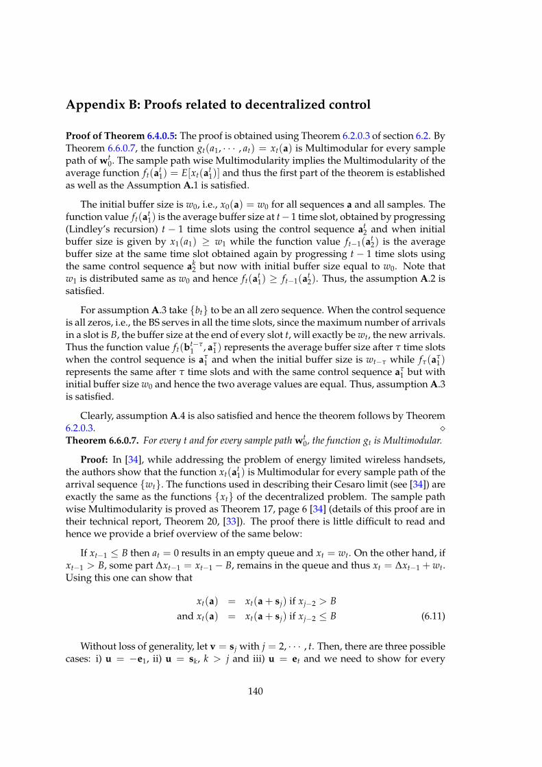
Appendix B: Proofs related to decentralized control

Proof of Theorem 6.4.0.5: The proof is obtained using Theorem 6.2.0.3 of section 6.2. ByTheorem 6.6.0.7, the function gt(a1, · · · , at) = xt(a) is Multimodular for every samplepath of wt

0. The sample path wise Multimodularity implies the Multimodularity of theaverage function ft(at

1) = E[xt(at1)] and thus the first part of the theorem is established

as well as the Assumption A.1 is satisfied.

The initial buffer size is w0, i.e., x0(a) = w0 for all sequences a and all samples. Thefunction value ft(at

1) is the average buffer size at t− 1 time slot, obtained by progressing(Lindley’s recursion) t − 1 time slots using the control sequence at

2 and when initialbuffer size is given by x1(a1) ≥ w1 while the function value ft−1(at

2) is the averagebuffer size at the same time slot obtained again by progressing t − 1 time slots usingthe same control sequence ak

2 but now with initial buffer size equal to w0. Note thatw1 is distributed same as w0 and hence ft(at

1) ≥ ft−1(at2). Thus, the assumption A.2 is

satisfied.

For assumption A.3 take bt to be an all zero sequence. When the control sequenceis all zeros, i.e., the BS serves in all the time slots, since the maximum number of arrivalsin a slot is B, the buffer size at the end of every slot t, will exactly be wt, the new arrivals.Thus the function value ft(bt−τ

1 , aτ1) represents the average buffer size after τ time slots

when the control sequence is aτ1 and when the initial buffer size is wt−τ while fτ(aτ

1)represents the same after τ time slots and with the same control sequence aτ

1 but withinitial buffer size w0 and hence the two average values are equal. Thus, assumption A.3is satisfied.

Clearly, assumption A.4 is also satisfied and hence the theorem follows by Theorem6.2.0.3. ⋄Theorem 6.6.0.7. For every t and for every sample path wt

0, the function gt is Multimodular.

Proof: In [34], while addressing the problem of energy limited wireless handsets,the authors show that the function xt(at

1) is Multimodular for every sample path of thearrival sequence wt. The functions used in describing their Cesaro limit (see [34]) areexactly the same as the functions xt of the decentralized problem. The sample pathwise Multimodularity is proved as Theorem 17, page 6 [34] (details of this proof are intheir technical report, Theorem 20, [33]). The proof there is little difficult to read andhence we provide a brief overview of the same below:

If xt−1 ≤ B then at = 0 results in an empty queue and xt = wt. On the other hand, ifxt−1 > B, some part ∆xt−1 = xt−1 − B, remains in the queue and thus xt = ∆xt−1 + wt.Using this one can show that

xt(a) = xt(a + sj) if xj−2 > B

and xt(a) = xt(a + sj) if xj−2 ≤ B (6.11)

Without loss of generality, let v = sj with j = 2, · · · , t. Then, there are three possiblecases: i) u = −e1, ii) u = sk, k > j and iii) u = et and we need to show for every

140

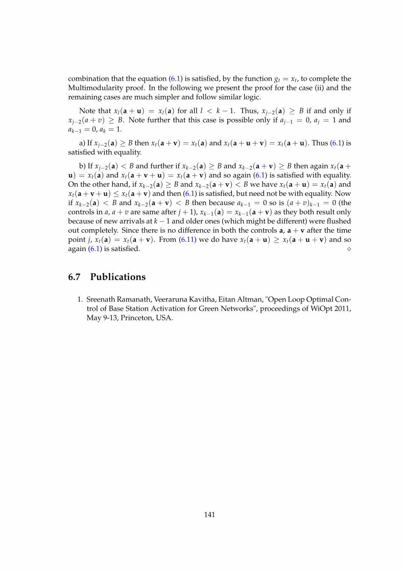
combination that the equation (6.1) is satisfied, by the function gt = xt, to complete theMultimodularity proof. In the following we present the proof for the case (ii) and theremaining cases are much simpler and follow similar logic.

Note that xl(a + u) = xl(a) for all l < k − 1. Thus, xj−2(a) ≥ B if and only ifxj−2(a + v) ≥ B. Note further that this case is possible only if aj−1 = 0, aj = 1 andak−1 = 0, ak = 1.

a) If xj−2(a) ≥ B then xt(a + v) = xt(a) and xt(a + u + v) = xt(a + u). Thus (6.1) issatisfied with equality.

b) If xj−2(a) < B and further if xk−2(a) ≥ B and xk−2(a + v) ≥ B then again xt(a +u) = xt(a) and xt(a + v + u) = xt(a + v) and so again (6.1) is satisfied with equality.On the other hand, if xk−2(a) ≥ B and xk−2(a + v) < B we have xt(a + u) = xt(a) andxt(a+ v+ u) ≤ xt(a+ v) and then (6.1) is satisfied, but need not be with equality. Nowif xk−2(a) < B and xk−2(a + v) < B then because ak−1 = 0 so is (a + v)k−1 = 0 (thecontrols in a, a + v are same after j + 1), xk−1(a) = xk−1(a + v) as they both result onlybecause of new arrivals at k − 1 and older ones (which might be different) were flushedout completely. Since there is no difference in both the controls a, a + v after the timepoint j, xt(a) = xt(a + v). From (6.11) we do have xt(a + u) ≥ xt(a + u + v) and soagain (6.1) is satisfied. ⋄

6.7 Publications

1. Sreenath Ramanath, Veeraruna Kavitha, Eitan Altman, "Open Loop Optimal Con-trol of Base Station Activation for Green Networks", proceedings of WiOpt 2011,May 9-13, Princeton, USA.

141

Part III

Resource Allocation

143

Chapter 7

Multiscale Fairness and itsApplication in Wireless Networks


7.2 Resource Sharing model and different fairness definitions . . . . . . 147

7.3 Instantaneous α-fairness for linear resources . . . . . . . . . . . . . . 153

7.4 Application to spectrum allocation in random fading channels . . . . 155

7.5 Application to indoor-outdoor scenario . . . . . . . . . . . . . . . . . . 160

7.6 Conclusion and Future Research . . . . . . . . . . . . . . . . . . . . . . 164

7.7 Publications . . . . . . . . . . . . . . . . . . . . . . . . . . . . . . . . . . 164

7.1 Introduction

Fair resource allocation is usually studied in a static context, in which a fixed amountof resources is to be shared. In dynamic resource allocation one usually tries to assignresources instantaneously so that the average share of each user is split fairly. The exactdefinition of the average share may depend on the application, as different applicationsmay require averaging over different time periods or time scales. We study dynamicresource allocation and examine how the constraints on the averaging durations impactthe amount of resources that each user gets.

Let us consider some set S of resource that we wish to distribute among I usersby assigning user i a subset Si of it. We shall be interested in allocating subsets of theresource fairly among the users. The set S may actually correspond to one or to severalresources. We shall consider standard fairness criteria for sharing the resources amongusers. We shall see, however, that the definition of a resource will have a major impacton the fair assignment.

145

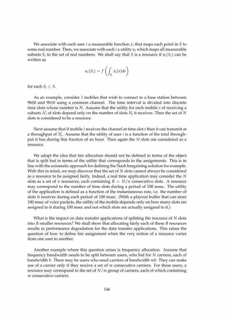
We associate with each user i a measurable function xi that maps each point in S tosome real number. Then, we associate with each i a utility ui which maps all measurablesubsets Si to the set of real numbers. We shall say that S is a resource if ui(Si) can bewritten as

ui(Si) = f

(

∫

Si

xi(s)ds

)

for each Si ⊂ S.

As an example, consider I mobiles that wish to connect to a base station between9h00 and 9h10 using a common channel. The time interval is divided into discretetime slots whose number is N. Assume that the utility for each mobile s of receiving asubsets Ni of slots depend only on the number of slots Ni it receives. Then the set of Nslots is considered to be a resource.

Next assume that if mobile i receives the channel at time slot t then it can transmit ata throughput of Xi

t. Assume that the utility of user i is a function of the total through-put it has during this fraction of an hour. Then again the N slots are considered as aresource.

We adopt the idea that fair allocation should not be defined in terms of the objectthat is split but in terms of the utility that corresponds to the assignments. This is inline with the axiomatic approach for defining the Nash bargaining solution for example.With this in mind, we may discover that the set of N slots cannot always be consideredas a resource to be assigned fairly. Indeed, a real time application may consider the Nslots as a set of n resources, each containing B = N/n consecutive slots. A resourcemay correspond to the number of time slots during a period of 100 msec. The utilityof the application is defined as a function of the instantaneous rate, i.e. the number ofslots it receives during each period of 100 msec. (With a playout buffer that can store100 msec of voice packets, the utility of the mobile depends only on how many slots areassigned to it during 100 msec and not which slots are actually assigned to it.)

What is the impact on data transfer applications of splitting the resource of N slotsinto B smaller resources? We shall show that allocating fairly each of these B resourcesresults in performance degradation for the data transfer applications. This raises thequestion of how to define fair assignment when the very notion of a resource variesfrom one user to another.

Another example where this question arises is frequency allocation. Assume thatfrequency bandwidth needs to be split between users, who bid for N carriers, each ofbandwidth b. There may be users who need carriers of bandwidth mb. They can makeuse of a carrier only if they receive a set of m consecutive carriers. For these users, aresource may correspond to the set of N/m group of carriers, each of which containingm consecutive carriers.

146

Related work

Our work is based on the α-fairness notion introduced by Mo and Walrand [105]. Thisnotion provides a continuum of fairness definitions through the real parameter α and itincludes various known fairness concepts that are obtained for some specific values ofthe real parameter α (the max-min fairness, the proportional fairness and the harmonicfairness). This, as well as other fairness notions can be defined through a set of axioms,see [94]. This work is inspired by several papers which already observed or derivedfairness at different time-scales [7, 5, 6, 37, 113, 91]. However, we would like to mentionthat the T-scale fairness (a unifying generalization of long- and short- term fairness)and multiscale fairness are new concepts introduced in the present work.

Structure of the chapter

The chapter is organized as follows: In the next Section 7.2 we introduce a resourcesharing model which is particularly suitable for wireless network applications. In Sec-tion 7.2 we also define several fairness criteria, illustrate them by examples and provetheoretical properties of the introduced fairness criteria. In Section 7.3 we derive ex-plicit formulae for instantaneous α-fairness in the case of linear resources. The case oflinear resources corresponds to the frequency as a resource in wireless networks. InSections 7.4 and 7.5 we apply different fairness criteria to spectrum allocation in fad-ing channels and to indoor-outdoor scenario, respectively. Section 7.6 concludes thechapter and provides avenues for future research.

7.2 Resource Sharing model and different fairness definitions

Consider n mobiles located at points x1, x2, ..., xn, respectively. We assume that the util-ity Ui of mobile i depends on its location xi and on the amount of resources si it gets.

Let S be the set of assignments; an assignment s ∈ S is a function from the vectorx to a point in the n-dimensional simplex. Its ith component, si(x) is the fraction ofresource assigned to mobile i.Definition 7.2.0.8. (α-fair assignment) An assignment s is α-fair if it is a solution of:

Z(x, α) := maxs

∑i

Zi(si, xi, α)

s.t. ∑i

si = 1, si ≥ 0∀i = 1, ..., n (7.1)

where,

Zi(xi, si, α) :=(Ui(xi, si))

1−α

1 − α

for α 6= 1. For α = 1 we define

Zi(xi, si, α) := log(Ui(xi, si))

147

We shall assume throughout that Ui is non-negative, strictly increasing and is con-cave in si. Then for any α > 0, Zi(xi, si, α) is strictly concave in si. We conclude thatZ(xi, si, α) is strictly concave in s for any α > 0 and therefore there is a unique solutions∗(α) to (7.1).Definition 7.2.0.9. (Mo and Walrand [105]) We call Zi(si, ·, α) the fairness utility of mobile iunder si, and we call Z(s, ·, α) the instantaneous degree of α-fairness under s.

In applications, the state X will be random, so that the instantaneous amount ofresource assigned by an α-fair allocation will also be a random variable. Thus, in addi-tion to instantaneous fairness we shall be interested in the expected amount assignedby being fair at each instant.Definition 7.2.0.10. We call E[Z(s, X, α)] the expected instantaneous degree of α-fairness un-der s.

In Section 7.2.1 we introduce the expected long-term fairness in which the expectedamount of resource is assigned fairly.Definition 7.2.0.11. We say that a utility is linear in the resource if it has the form:

Ui(xi, si) := siqi(xi).

For example, consider transmission between a mobile source and a base station, andassume(i) that the base station is in the origin (x = 0) but at a height of one unit, whereasall mobiles are on the ground and have height 0. Thus, the distance between the base

station and a mobile located on the ground at point x is√

1 + ||x||2.(ii) that the Shannon capacity can be used to describe the utility. If the resource that isshared is the frequency then the utility has the linear form:

U(C, x) := Cq(x)

where q(x) = log(

1 +P(x2 + 1)−β/2

σ2

)

Note: if the power and not the frequency, were taken to be the resource then wewould not obtain the linear form of the resource.

In the linear case, we write Zi as:

Zi(s, x, α) := s1−αi vi(x), vi :=

(qi(xi))1−α

1 − α

7.2.1 Fairness over time: Instantaneous Versus Long term α-fairness

Next we consider the case where xi(t), i = 1, ..., n, may change in time.

148

Definition 7.2.1.1. We define an assignment to be instantaneous α-fair if at each time t eachmobile is assigned a resource so as to be α-fair at that instant.

Consider the instantaneous α-fair allocation and assume that time is discrete. Wethus compute the instantaneous α-fair fair assignment over a period of T slot as theassignment that maximizes (for α 6= 1)

n

∑i=1

(Ui(xi(t), si(t)))1−α

1 − α.

for every t = 1, ..., T. This is equivalent to maximizing

T

∑t=1

n

∑i=1


1 − α. (7.2)

For α = 1 the same is true but where we replace


1 − α

bylog[Ui(xi(t), si(t))]

We make the following surprising observation: The optimization problem (7.2) corre-sponds to the α-fair assignment problem in which there are nT players instead of nplayers, where the utility of player i = kn + j (k = 0, ..., T − 1, j = 1, ..., n) is defined as

Ui(xi, si) = Uj(xj(k + 1), sj(k + 1))

. Thus the expected instantaneous fairness criterion in the stationary and ergodic caseregards assignments at different time slots of the same player as if it were a differentplayer at each time slot!

Note that when considering the proportional fair assignment, then the resultingassignment is the one that maximizes

n

∏i=1

T

∏t=1

Ui(xi(t), si(t))

Definition 7.2.1.2. Assume that the state process X(t) is stationary ergodic. Let λi be thestationary probability measure of X(0). The long term α-fairness index of an assignment s ∈ Sof a stationary process X(t) is defined as

Zλ(s) :=n

∑i=1

Ziλ(s)

where Ziλ(s) =

(

Eλ [Ui(Xi(0), si(X(0)))])1−α

1 − α

An assignment s is long-term α-fair if it maximizes Zλ(s) over s ∈ S.

149

As we see, instead of attempting to have a fair assignment of the resources at everyt, it is the expected utility in the stationary regime that one assigns fairly according tothe the long-term fairness. Under stationarity and ergodicity conditions on the processX(t) this amounts in an instantaneous assignment of the resources in a way that thetime average amount allocated to the users are α-fair.

7.2.2 Fairness over time: T-scale α-fairness

Next we define fairness concepts that are in between the instantaneous and the ex-pected fairness. They are related to fairness over a time interval T. Either continuoustime is considered or discrete time where time is slotted and each slot is considered tobe of one time unit. Below, we shall understand the integral to mean summation whenever time is discrete.Definition 7.2.2.1. The T-scale α-fairness index of an assignment s ∈ S is defined as

ZT(s) :=n

∑i=1

ZiT(s)

where ZiT =

[

1T

∫ T0 Ui(Xi(t), si(X(t)))dt

]1−α

1 − α

The expected T-scale α-fairness index is its expectation. An assignment s is T-scale α-fair if itmaximizes ZT(s) over s ∈ S.Definition 7.2.2.2. The T-scale expected α-fairness index of an assignment s ∈ S is defined as

ZT(s) :=n

∑i=1

ZiT(s)

where ZiT =

[

1T

∫ T0 E[Ui(Xi(t), si(X(t)))]dt

]1−α

1 − α

We shall consider the following simple example of 2-scale fairnessExample 7.2.2.3. Consider two time slots and two mobile stations. To whoever the first timeslot will be allocated, that mobile would send or receive 25 units. At the second slot, a rate of 5(resp. 10) units will be used if the slot is assigned to mobile 1 (resp. 2). We make the followingobservations. By [i,j] we shall denote the allocation that assigns slot 1 to mobile i and slot 2to mobile j. The allocation [1,2] maximizes the global utility and moreover, the α-fair 2-scaleutility for any α.

Thus, we observe that the α-assignment is not monotone: The player with largerutilities received less at the α-fair utility, for all values of α!Example 7.2.2.4. (Example 7.2.2.3 continued) We now change a single utility in the last ex-ample: assume that if mobile 2 receives the first slot then it earns 102 units.

(i) Now the global optimal solution is the assignment [2,2].

(ii) The proportional fair solution (α = 1) is [2,1].

150

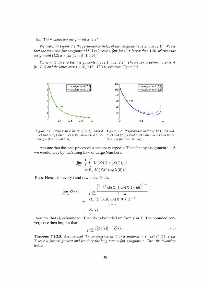
(iii) The maxmin fair assignment is [1,2].

We depict in Figure 7.1 the performance index of the assignments [1,2] and [2,1]. We seethat the max-min fair assignment [2,1] is 2-scale α-fair for all α larger than 1.36, whereas theassignment [1,2] is α fair for α ∈ [1, 1.36].

For α < 1 the two best assignments are [2,1] and [2,2]. The former is optimal over α ∈[0.17, 1] and the latter over α ∈ [0, 0.17]. This is seen from Figure 7.2.

1.4 1.6 1.8 20

1

2

3

4

5

6

assignment [2,1]assignment [1,2]

1.36

Figure 7.1: Performance index of [2,1] (dashedline) and [1,2] (solid line) assignments as a func-tion of α (horizontal axis)

0 0.5 10

20

40

60

80

100

120

assignment [2,2]assignment [2,1]

0.17

Figure 7.2: Performance index of [2,1] (dashedline) and [2,2] (solid line) assignments as a func-tion of α (horizontal axis)

Assume that the state processes is stationary ergodic. Then for any assignment s ∈ Swe would have by the Strong Law of Large Numbers:

limT→∞

1T

∫ T

0Ui(Xi(t), si(X(t)))dt

= Eλ [Ui(Xi(0), si(X(0)))]

P-a.s. Hence, for every i and s, we have P-a.s.

limT→∞

ZiT(s) = lim

T→∞

[

1T

∫ T0 Ui(Xi(t), si(X(t)))dt

]1−α

1 − α

=(Eλ [Ui(Xi(0), si(X(0)))])1−α

1 − α

= ZiT(s).

Assume that Ui is bounded. Then ZiT is bounded uniformly in T. The bounded con-

vergence then implies that

limT→∞

E[ZiT(s)] = Z

iT(s). (7.3)

Theorem 7.2.2.5. Assume that the convergence in (7.3) is uniform in s. Let s∗(T) be theT-scale α fair assignment and let s∗ be the long term α-fair assignment. Then the followingholds:

151

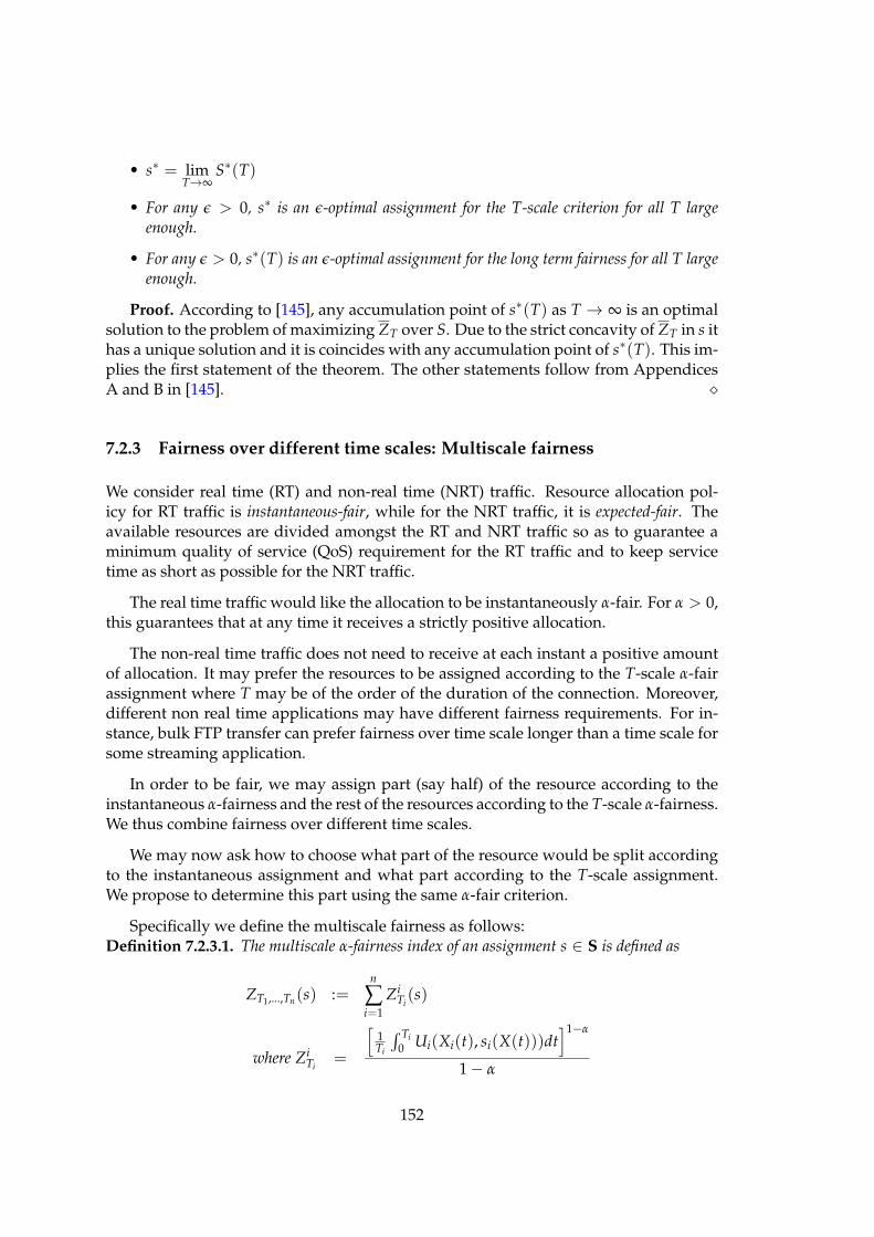
• s∗ = limT→∞

S∗(T)

• For any ǫ > 0, s∗ is an ǫ-optimal assignment for the T-scale criterion for all T largeenough.

• For any ǫ > 0, s∗(T) is an ǫ-optimal assignment for the long term fairness for all T largeenough.

Proof. According to [145], any accumulation point of s∗(T) as T → ∞ is an optimalsolution to the problem of maximizing ZT over S. Due to the strict concavity of ZT in s ithas a unique solution and it is coincides with any accumulation point of s∗(T). This im-plies the first statement of the theorem. The other statements follow from AppendicesA and B in [145]. ⋄

7.2.3 Fairness over different time scales: Multiscale fairness

We consider real time (RT) and non-real time (NRT) traffic. Resource allocation pol-icy for RT traffic is instantaneous-fair, while for the NRT traffic, it is expected-fair. Theavailable resources are divided amongst the RT and NRT traffic so as to guarantee aminimum quality of service (QoS) requirement for the RT traffic and to keep servicetime as short as possible for the NRT traffic.

The real time traffic would like the allocation to be instantaneously α-fair. For α > 0,this guarantees that at any time it receives a strictly positive allocation.

The non-real time traffic does not need to receive at each instant a positive amountof allocation. It may prefer the resources to be assigned according to the T-scale α-fairassignment where T may be of the order of the duration of the connection. Moreover,different non real time applications may have different fairness requirements. For in-stance, bulk FTP transfer can prefer fairness over time scale longer than a time scale forsome streaming application.

In order to be fair, we may assign part (say half) of the resource according to theinstantaneous α-fairness and the rest of the resources according to the T-scale α-fairness.We thus combine fairness over different time scales.

We may now ask how to choose what part of the resource would be split accordingto the instantaneous assignment and what part according to the T-scale assignment.We propose to determine this part using the same α-fair criterion.

Specifically we define the multiscale fairness as follows:Definition 7.2.3.1. The multiscale α-fairness index of an assignment s ∈ S is defined as

ZT1,...,Tn(s) :=n

∑i=1

ZiTi(s)

where ZiTi

=

[

1Ti

∫ Ti

0 Ui(Xi(t), si(X(t)))dt]1−α

1 − α

152

The expected multiscale α-fairness index is its expectation. An assignment s is multiscale α-fair if it maximizes ZT1,...,Tn(s) over s ∈ S. We also say that multiscale α-fair assignment is(T1, ..., Tn)-scale fair assignment.Example 7.2.3.2. Let us consider an example of multiscale fairness. Say, we have in total Ntime slots. The allocation happens in a bundle of 6 slots, such that, either we allocate all of it toan outdoor user located at x1 or fair share them amongst 3 indoor users located at (y1, y2, y3)with yi ∈ (0, L), with any user getting two consecutive slots. Now the question is "Given thatwe fair-share among the indoor users, how do we fair share between the outdoor and the indoorusers?".

In this example, we assume any user gets a throughput q ∈ [0, 1]. Let U1, U2, representthe utility of user 1 and sum utility of users 2− 4 and let T1, 1− T1 represent their respectiveassignment of resources. Now, utility of user 1,

U1(T1) = 6T1q1(x1).

Let s = s1, s2, 1 − s1 − s2 represent the assignment of resources for the indoor users. Then,utility of users 2 − 4 is

u2(T1, s) = 6s1(1 − T1)q2(y2),

u3(T1, s) = 6s2(1 − T1)q3(y3)

and

u4(T1, s) = 6(1 − s1 − s2)(1 − T1)q4(y4)

Now the α-fair share s∗ = s∗1 , s∗2 , 1 − (s∗1 − s∗2) is given by,

s∗ = arg maxs

4

∑i=2

E[ui(T1, s)]1−α1

1 − α1

The sum utility of users 2 − 4 is,

U2(T1) =4

∑i=2

6si∗(1 − T1)qi(yi)

The α-fair share between the outdoor and indoor users is,

T∗1 = arg max

T1

E [U1(T1)]1−α + E [U2(1 − T1)]

1−α

1 − α

7.3 Instantaneous α-fairness for linear resources

In the case of linear resources the instantaneous α-fairness has a nice explicit expression.

153

Theorem 7.3.0.3. (i) The α-fair share is given by

s∗i =vi(xi)

1/α

∑j vj(xj)1/α=

qi(xi)1/α−1

∑j qj(xj)1/α−1

(ii) The utility for mobile i under the fair assignment is then

Ui(s∗, x) =

vi(xi)1/α

∑j vj(xj)1/αqi(xi) =

qi(xi)1/α

∑j qj(xj)1/α−1

(iii) The optimal value Z is given by

Z =1

1 − α ∑i

(

qi(xi)1+1/α

∑j qj(xj)1/α

)1−α

Proof. We relax the constraint and use KKT condition. s is optimal if and only ifthere is some λ > 0 such that s maximize Lλ s.t. si ≥ 0 for all i, where

Lλ = ∑i

s1−αi vi + λ(1 − ∑

i

si)

Equating the derivative w.r.t. si to zero gives

s−αi vi(xi) =

λ

1 − α

so that si =

(

1 − α

λvi(xi)

)1/α

Since the sum of si is 1, we conclude that

λ

1 − α=

(

∑j

vj(xj)1/α

)α

Substituting in the previous equation yields (i), which then implies the rest. ⋄Example 7.3.0.4. Consider as an example a path loss β = 2 and let the base station be locatedone unit above the mobiles. We assume that qi(x) is proportional to the attenuation between themobile and the base station: qi(x) = ciq(x) where q(x) = (1 + x2)−1/2. For β = α = 2 wehave

s∗i (x) =c−1/2

i (1 + x2i )

−1/2

∑j c−1/2j (1 + x2

j )−1/2

.

Furthermore,

Ui(s∗, x) = s∗i (x)qi(xi) =

c1/2i (1 + x2

i )

∑j c−1/2j

√

1 + x2j

.

154

7.4 Application to spectrum allocation in random fading chan-nels

We consider two users: fast-changing user and slowly-changing user. The users’ chan-nels are modeled by the Gilbert model. The users can be either in a good or in abad state. The dynamics of the fast-changing user is described by a Markov chainY1(t)t=0,1,... with the following transition matrix

P1 =

[

1 − α1 α1β1 1 − β1

]

.

Its stationary distribution is given by

π1 =

[

β1

α1 + β1

α1

α1 + β1

]

.

The slowly-changing user is described by a Markov chain Y2(t)t=0,1,... with the fol-lowing transition matrix

P2 =

[

1 − ǫα2 ǫα2ǫβ2 1 − ǫβ2

]

.

Its stationary distribution is given by

π2 =

[

β2

α2 + β2

α2

α2 + β2

]

.

Note that the parameter ǫ does not have an effect on the stationary distribution but itinfluences for how long the slowly-changing user stays in some state. The smaller ǫ, themore seldom the user changes the states. If we choose α1 = α2 and β1 = β2, then thefast-changing user and the slowly-changing user have the same stationary distribution.

We assume that state 1 is a bad state and state 2 is a good state. When the fast-changing user is in the bad state, its channel gain coefficient is h11 and when the fast-changing user is in the good state, its channel gain coefficient is h12. Of course, we haveh11 < h12. Thus, the achievable throughputs in different states are given by

U11 = s11q11 = s11 log(

1 +h11P1

σ2

)

,

U12 = s12q12 = s12 log(

1 +h12P1

σ2

)

where P1 is the power applied by the fast-changing user.

Similarly, for the slowly-changing user we associate with the bad state (state 1) thechannel gain h21 and with the good state (state 2) the channel gain h22. Again we haveh21 < h22, and the achievable throughputs in different states are given by

U21 = s21q21 = s21 log(

1 +h21P2

σ2

)

,

U12 = s22q22 = s22 log(

1 +h22P2

σ2

)

155

where P2 is the power applied by the slowly-changing user.

First, we would like to analyze T-scale fairness and to see the effect of the timescale on the resource allocation. Specifically, we consider the following optimizationcriterion

2

∑i=1

11 − α

[

1T

T

∑t=0

Ui(t)

]1−α

→ maxs1,s2

(7.4)

with Ui(t) = si(t)qi,Yi(t) and s1(t) + s2(t) = 1.

Let us consider several options for the time horizon T:

Instantaneous fairness. If we take T = 1 we obtain the instantaneous fairness. Namely,the criterion (7.4) takes the form

11 − α

[

U1−α1 (0) + U1−α

2 (0)]

→ maxs1,s2

The solution of the above optimization problem (follows from Theorem 1) is given by

si(0) =q(1−α)/α

i,Yi(0)

q(1−α)/α

1,Y1(0)+ q

(1−α)/α

2,Y2(0)

This allocation results in the following expected throughputs

θ1 = ∑i,j

q1/α1,i

q(1−α)/α1,i + q

(1−α)/α2,j

π1,iπ2,j,

θ2 = ∑i,j

q1/α2,j

q(1−α)/α1,i + q

(1−α)/α2,j

π1,iπ2,j. (7.5)

Mid-term fairness. Let us take the time horizon as a function of the underlying dy-namics time parameter ǫ, that is T = T(ǫ), satisfying the following conditions: (a)T(ǫ) → ∞ and (b) T(ǫ)ǫ → 0. The condition (a) ensures that

1T(ǫ)

T(ǫ)

∑t=0

1Y1(t) = i → π1,i, as ǫ → 0,

and the condition (b) ensures that

1T(ǫ)

T(ǫ)

∑t=0

1Y2(t) = i → δY2(0),i, as ǫ → 0.

This follows from the theory of Markov chains with multiple time scales (see e.g., [58]).It turns out to be convenient to take the following notation for the resource allocation:We denote by s(t) the allocation for the fast-changing user and by 1 − s(t) the resource

156

allocation for the slowly-changing user. Thus, we have s1(t) = s(t) and s2(t) = 1− s(t).We denote by si,j = E[s(t)|Y1(t) = i, Y2(t) = j]. We note that since the fast-changinguser achieves stationarity when T(ǫ) → ∞ we are able to solve (7.4) in stationary strate-gies. Then, the criterion (7.4) takes the form

11 − α

[

(π1,1q1,1s1,Y2(0) + π1,2q1,2s2,Y2(0))1−α

+ ((1 − π1,1s1,Y2(0) − π1,2s2,Y2(0))q2,Y2(0))1−α]

→ maxs1,Y2(0)

, s2,Y2(0)

The above nonlinear optimization problem can be solved numerically. The expectedthroughputs in the mid-term fairness case are given by

θ1 = (π1,1q1,1s1,1 + π1,2q1,2s2,1)π2,1

+ (π1,1q1,1s1,2 + π1,2q1,2s2,2)π2,2

θ2 = (1 − π1,1s1,1 − π1,2s2,1)q2,1π2,1

+ (1 − π1,1s1,2 − π1,2s2,2)q2,2π2,2 (7.6)

Long-term fairness. In the case of long-term fairness we set T = ∞ which results in thefollowing criterion

11 − α

[

E[U1]1−α + E[U2]

1−α]

→ maxs1,s2

Due to stationarity, we can solve the above optimization problem over sequences instationary strategies. Namely, we have the following optimization problem

11 − α

((π1,1π2,1s1,1 + π1,1π2,2s1,2)q1,1

+ (π1,2π2,1s2,1 + π1,2π2,2s2,2)q1,2)1−α

+ ((π2,1 − π1,1π2,1s1,1 − π1,2π2,1s2,1)q2,1

+ (π2,2 − π1,1π2,1s1,1 − π1,2π2,2s2,2)q2,2)1−α]

→ maxs1,1, s1,2, s2,1, s2,2

The expected throughputs in the long-term fairness case are given by

θ1 = (π1,1π2,1s1,1 + π1,1π2,2s1,2)q1,1

+ (π1,2π2,1s2,1 + π1,2π2,2s2,2)q1,2

θ2 = (π2,1 − π1,1π2,1s1,1 − π1,2π2,1s2,1)q2,1

+ (π2,2 − π1,1π2,1s1,1 − π1,2π2,2s2,2)q2,2 (7.7)

Let us also consider the expected instantaneous fairness which is given by the criterion

11 − α

[

E[U1−α1 (t)] + E[U1−α

2 (t)]]

→ maxs1,s2

157

which is equivalent to

11 − α

[

∑ij

π1,iπ2,j

∫ 1

0(sq1,i)

1−αdFij(s)

+∑ij

π1,iπ2,j

∫ 1

0((1 − s)q2,j)

1−αdFij(s)

]

→ maxFij

where Fij(s) is the distribution for s(t) conditioned on the event Y1(t) = i, Y2(t) = j.The above criterion is maximized by

Fij(s) =

0, if s < q(1−α)/α1,i /(q(1−α)/α

1,i + q(1−α)/α2,j ),

1, if s ≥ q(1−α)/α1,i /(q(1−α)/α

1,i + q(1−α)/α2,j ).

Thus, we can see that the expected instantaneous fairness criterion is equivalent toinstantaneous fairness.

Let us consider a numerical example. The parameters are given in Table 1. We con-sider three typical cases. For these three cases, we plot the expected throughput of themobiles for various fairness criteria (see Figures 7.3-7.5). The first case corresponds tothe symmetric scenario. Since in this scenario the users have the same stationary dis-tributions and the same conditional Shannon capacities, the expected throughputs arethe same when we use either instantaneous fairness criterion or long-term fairness cri-terion. Interesting, in the long-term fairness case, both users experience degradation inthroughput when α increases. In the case of mid-term fairness, the expected through-put of the fast-changing user is higher as in the mid-term fairness criterion the utilityof the fast-changing user is the α-fairness function of the expected throughput. In thesecond case, the fast-changing user has in general better channel conditions. In thiscase, different fairness criteria provide different resource allocation. We observe thatinstantaneous and mid-term fairness allocations are more sensitive with respect to theparameter α than the long-term fairness allocation. In the third scenario the slowly-changing user (user 2) is more often in the good channel state than the fast-changinguser (user 1). Now, for all the criteria the slowly-changing user has better expectedthroughput.

Next, let us consider multiscale fairness over time. Specifically, (T1, T2)-scale fair-ness is defined by the following criterion

11 − α

(

1T1

T1

∑t=0

U1(t)

)1−α

+

(

1T2

T2

∑t=0

U2(t)

)1−α

→ maxs1,s2

In this particular example, there are 6 possible combinations of different time scales.It turns out that in this example only the (1, ∞)-scale fairness gives a new resourceallocation. The other combinations of time scales reduce to some T-scale fairness. Thus,let us first consider the multiscale fairness when we apply instantaneous fairness to the

158

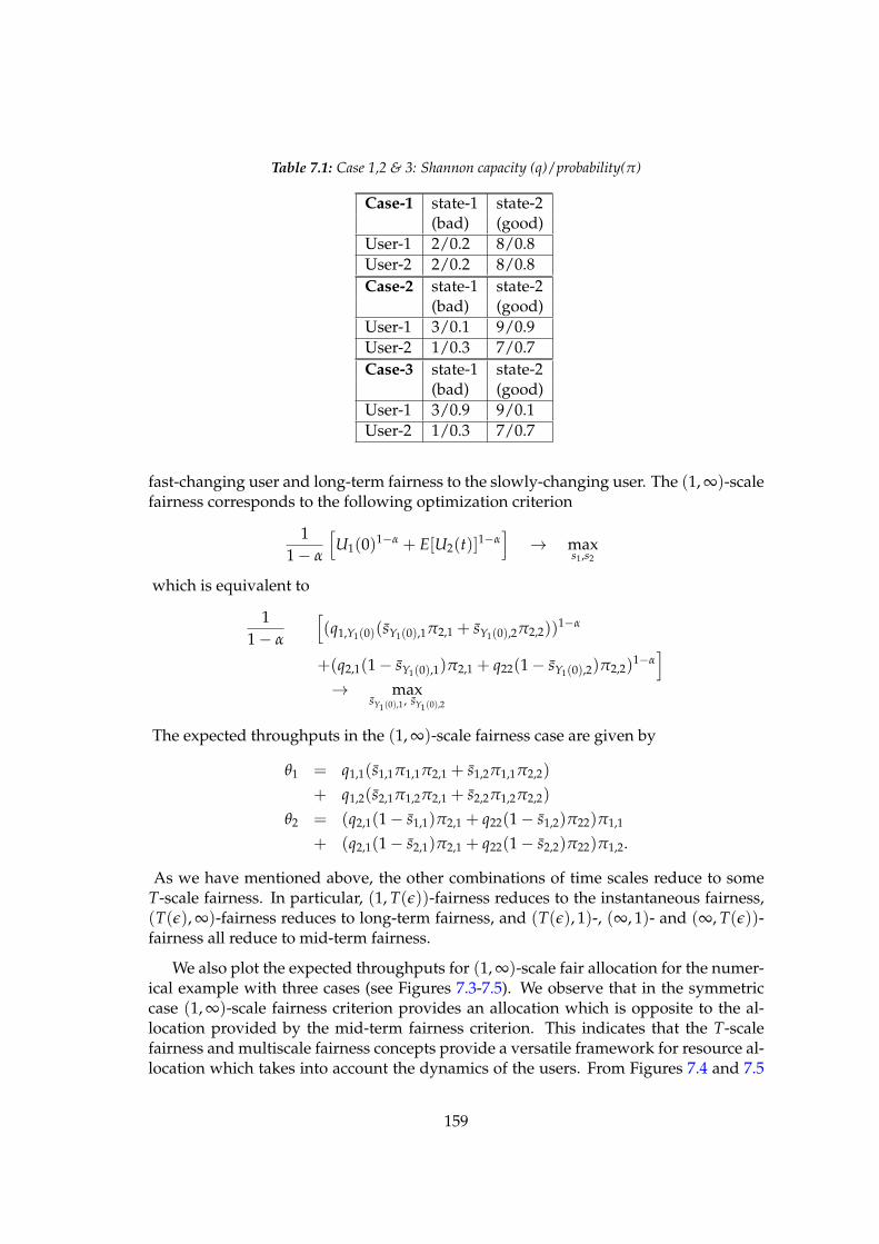
Table 7.1: Case 1,2 & 3: Shannon capacity (q)/probability(π)

Case-1 state-1 state-2(bad) (good)

User-1 2/0.2 8/0.8User-2 2/0.2 8/0.8Case-2 state-1 state-2

(bad) (good)User-1 3/0.1 9/0.9User-2 1/0.3 7/0.7Case-3 state-1 state-2

(bad) (good)User-1 3/0.9 9/0.1User-2 1/0.3 7/0.7

fast-changing user and long-term fairness to the slowly-changing user. The (1, ∞)-scalefairness corresponds to the following optimization criterion

11 − α

[

U1(0)1−α + E[U2(t)]1−α]

→ maxs1,s2

which is equivalent to

11 − α

[

(q1,Y1(0)(sY1(0),1π2,1 + sY1(0),2π2,2))1−α

+(q2,1(1 − sY1(0),1)π2,1 + q22(1 − sY1(0),2)π2,2)1−α]

→ maxsY1(0),1

, sY1(0),2

The expected throughputs in the (1, ∞)-scale fairness case are given by

θ1 = q1,1(s1,1π1,1π2,1 + s1,2π1,1π2,2)

+ q1,2(s2,1π1,2π2,1 + s2,2π1,2π2,2)

θ2 = (q2,1(1 − s1,1)π2,1 + q22(1 − s1,2)π22)π1,1

+ (q2,1(1 − s2,1)π2,1 + q22(1 − s2,2)π22)π1,2.

As we have mentioned above, the other combinations of time scales reduce to someT-scale fairness. In particular, (1, T(ǫ))-fairness reduces to the instantaneous fairness,(T(ǫ), ∞)-fairness reduces to long-term fairness, and (T(ǫ), 1)-, (∞, 1)- and (∞, T(ǫ))-fairness all reduce to mid-term fairness.

We also plot the expected throughputs for (1, ∞)-scale fair allocation for the numer-ical example with three cases (see Figures 7.3-7.5). We observe that in the symmetriccase (1, ∞)-scale fairness criterion provides an allocation which is opposite to the al-location provided by the mid-term fairness criterion. This indicates that the T-scalefairness and multiscale fairness concepts provide a versatile framework for resource al-location which takes into account the dynamics of the users. From Figures 7.4 and 7.5

159

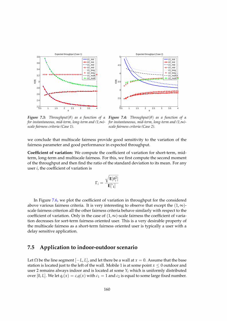
0.5 1 1.5 2 2.5 3 3.5 42.2

2.4

2.6

2.8

3

3.2

3.4

3.6

3.8Expected throughput (Case 1)

α

E[θ

]

U1_instU2_instU1_midU2_midU1_longU2_longU1_multiU2_multi

Figure 7.3: Throughput(θ) as a function of αfor instantaneous, mid-term, long-term and (1,∞)-scale fairness criteria (Case 1).

0.5 1 1.5 2 2.5 3 3.5 42

2.5

3

3.5

4

4.5

5Expected throughput (Case 2)

α

E[θ

]



we conclude that multiscale fairness provide good sensitivity to the variation of thefairness parameter and good performance in expected throughput.

Coefficient of variation: We compute the coefficient of variation for short-term, mid-term, long-term and multiscale fairness. For this, we first compute the second momentof the throughput and then find the ratio of the standard deviation to its mean. For anyuser i, the coefficient of variation is

Γi =

√

E[θ2i ]

E[`i]

In Figure 7.6, we plot the coefficient of variation in throughput for the consideredabove various fairness criteria. It is very interesting to observe that except the (1, ∞)-scale fairness criterion all the other fairness criteria behave similarly with respect to thecoefficient of variation. Only in the case of (1, ∞)-scale fairness the coefficient of varia-tion decreases for sort-term fairness oriented user. This is a very desirable property ofthe multiscale fairness as a short-term fairness oriented user is typically a user with adelay sensitive application.

7.5 Application to indoor-outdoor scenario

Let Ω be the line segment [−L, L], and let there be a wall at x = 0. Assume that the basestation is located just to the left of the wall. Mobile 1 is at some point x ≤ 0 outdoor anduser 2 remains always indoor and is located at some Yt which is uniformly distributedover [0, L]. We let qi(x) = ciq(x) with c1 = 1 and c2 is equal to some large fixed number.

160

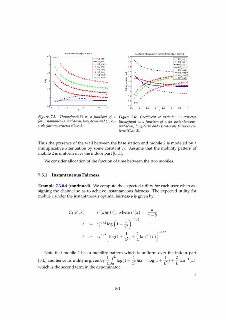
0.5 1 1.5 2 2.5 3 3.5 41.5

2

2.5

3

3.5

4

4.5Expected throughput (Case 3)

α

E[θ

]



0.5 1 1.5 2 2.5 3 3.5 40.7

0.8

0.9

1

1.1

1.2

1.3

1.4

1.5

1.6

1.7Coefficient of variation in expected throughput (Case 3)

α

Cff

t o

f va

ria

tion

in θ


Figure 7.6: Coefficient of variation in expectedthroughput as a function of α for instantaneous,mid-term, long-term and (1,∞)-scale fairness cri-teria (Case 3).

Thus the presence of the wall between the base station and mobile 2 is modeled by amultiplicative attenuation by some constant c2. Assume that the mobility pattern ofmobile 2 is uniform over the indoor part [0, L].

We consider allocation of the fraction of time between the two mobiles.

7.5.1 Instantaneous Fairness

Example 7.3.0.4 (continued). We compute the expected utility for each user when as-signing the channel so as to achieve instantaneous fairness. The expected utility formobile 1 under the instantaneous optimal fairness s is given by

U1(s∗, x) = s∗(x)q1(x), where s∗(x) :=

a

a + b

a := c−1/21 log

(

1 +1x2

)−1/2

b := c−1/22

[

log(1 +1L2 ) +

2L

tan−1(L)

]−1/2

Note that mobile 2 has a mobility pattern which is uniform over the indoor part

[0,L] and hence its utility is given by1L

∫ L

0log(1 +

1x2 )dx = log(1 +

1L2 ) +

2L

tan−1(L),

which is the second term in the denominator.

⋄

161

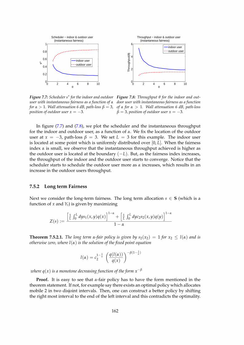
0 2 4 6 8 100

0.2

0.4

0.6

0.8

1

Scheduler − indoor & outdoor user (instantaneous fairness)

α

s*

indoor useroutdoor user

Figure 7.7: Scheduler s∗ for the indoor and outdooruser with instantaneous fairness as a function of αfor α > 1. Wall attenuation 6 dB, path-loss β = 3,position of outdoor user x = −3.

0 2 4 6 8 100

2

4

6

Throughput − indoor & outdoor user (instantaneous fairness)

α

Th

rou

gh

pu

t(θ)

indoor useroutdoor user

Figure 7.8: Throughput θ for the indoor and out-door user with instantaneous fairness as a functionof α for α > 1. Wall attenuation 6 dB, path-lossβ = 3, position of outdoor user x = −3.

In figure (7.7) and (7.8), we plot the scheduler and the instantaneous throughputfor the indoor and outdoor user, as a function of α. We fix the location of the outdooruser at x = −3, path-loss β = 3. We set L = 3 for this example. The indoor useris located at some point which is uniformly distributed over [0, L]. When the fairnessindex α is small, we observe that the instantaneous throughput achieved is higher asthe outdoor user is located at the boundary (−L). But, as the fairness index increases,the throughput of the indoor and the outdoor user starts to converge. Notice that thescheduler starts to schedule the outdoor user more as α increases, which results in anincrease in the outdoor users throughput.

7.5.2 Long term Fairness

Next we consider the long-term fairness. The long term allocation s ∈ S (which is afunction of x and Yt) is given by maximizing

Z(s) :=

[

1L

∫ L0 dys1(x, y)q(x)

]1−α+[

1L

∫ L0 dyc2s2(x, y)q(y)

]1−α

1 − α

Theorem 7.5.2.1. The long term α-fair policy is given by s2(x2) = 1 for x2 ≤ l(α) and isotherwise zero, where l(α) is the solution of the fixed point equation

l(α) = c1− 1

α2

(

q(l(α))

q(x)

)−β(1− 1α )

where q(x) is a monotone decreasing function of the form x−β

Proof. It is easy to see that α-fair policy has to have the form mentioned in thetheorem statement. If not, for example say there exists an optimal policy which allocatesmobile 2 in two disjoint intervals. Then, one can construct a better policy by shiftingthe right most interval to the end of the left interval and this contradicts the optimality.

162

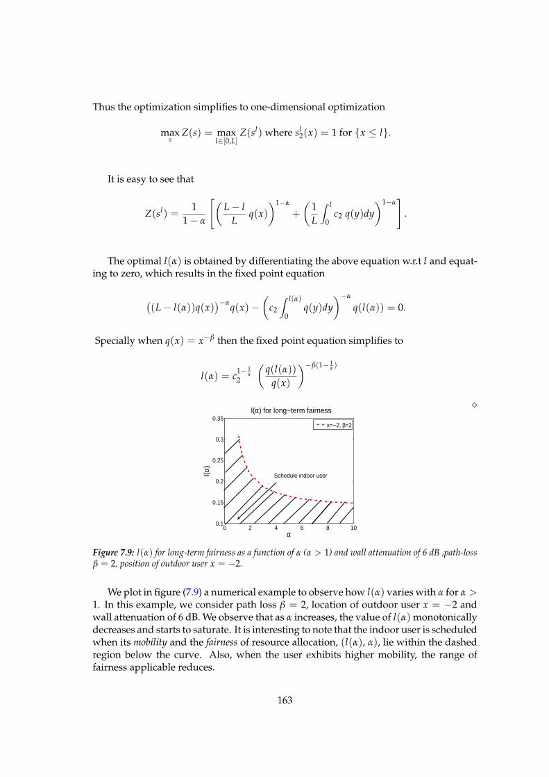
Thus the optimization simplifies to one-dimensional optimization

maxs

Z(s) = maxl∈[0,L]

Z(sl) where sl2(x) = 1 for x ≤ l.

It is easy to see that

Z(sl) =1

1 − α

[

(

L − l

Lq(x)

)1−α

+

(

1L

∫ l

0c2 q(y)dy

)1−α]

.

The optimal l(α) is obtained by differentiating the above equation w.r.t l and equat-ing to zero, which results in the fixed point equation

(

(L − l(α))q(x))−α

q(x)−(

c2

∫ l(α)

0q(y)dy

)−α

q(l(α)) = 0.

Specially when q(x) = x−β then the fixed point equation simplifies to

l(α) = c1− 1

α2

(

q(l(α))

q(x)

)−β(1− 1α )

⋄

0 2 4 6 8 100.1

0.15

0.2

0.25

0.3

0.35l(α) for long−term fairness

α

l(α)

x=−2, β=2

Schedule indoor user

Figure 7.9: l(α) for long-term fairness as a function of α (α > 1) and wall attenuation of 6 dB ,path-lossβ = 2, position of outdoor user x = −2.

We plot in figure (7.9) a numerical example to observe how l(α) varies with α for α >

1. In this example, we consider path loss β = 2, location of outdoor user x = −2 andwall attenuation of 6 dB. We observe that as α increases, the value of l(α) monotonicallydecreases and starts to saturate. It is interesting to note that the indoor user is scheduledwhen its mobility and the fairness of resource allocation, (l(α), α), lie within the dashedregion below the curve. Also, when the user exhibits higher mobility, the range offairness applicable reduces.

163

7.6 Conclusion and Future Research

We have introduced T-scale fairness and multiscale fairness. The notion of T-scale fair-ness allows one to address in a flexible manner requirements of emerging applications(like YouTube) which demand quality of service requirement between strict real timetraffic and best effort traffic. The notion of multiscale fairness allows one to use a singleoptimization criterion for resource allocation when different applications are present inthe network. We have compared the new fairness notions with previously known cri-teria of instantaneous and long-term fairness criteria. We have illustrated the new no-tions by their application in wireless networks. Specifically, we have considered spec-trum allocation when users with different dynamics are present in the system. We havedemonstrated that the multiscale fairness provides a versatile framework for resourceallocation. We have also considered the resource allocation in indoor-outdoor scenarioand have observed how the spacial component influences the resource scheduling un-der different fairness criteria. In the near future we plan to investigate in detail howmultiscale fairness criterion allocates resources when a number of applications withdifferent QoS requirements are present in the network. It is also interesting to investi-gate T-scale fairness in the non-stationary regime.

7.7 Publications

1. Eitan Altman, Konstantin Avrachenkov, Sreenath Ramanath, "Multiscale Fairnessand its Application to Resource Allocation in Wireless Networks", proceedings ofIFIP Networking 2011, LNCS 6631, May 9-13, Valencia, Spain.

2. Sreenath Ramanath, Eitan Altman, Konstantin Avrachenkov, "A heterogeneousapproach to fair resource allocation and its application in femtocell networks",proceedings of the Workshop on Indoor and Outdoor Femto Cells (IOFC’11), May13, Princeton USA.

3. Eitan Altman, Konstantin Avrachenkov, Sreenath Ramanath, "Multiscale Fairnessand its Networking Application", Poster, Performance 2010, Nov 17-19, Namur,Belgium.

164

Chapter 8

Satisfying Demands in MulticellNetworks: A Universal PowerAllocation Algorithm


8.2 System model . . . . . . . . . . . . . . . . . . . . . . . . . . . . . . . . . 167

8.3 System specific problem formulation . . . . . . . . . . . . . . . . . . . 169

8.4 Universal Algorithm : UPAMCN . . . . . . . . . . . . . . . . . . . . . 173

8.5 Simulation . . . . . . . . . . . . . . . . . . . . . . . . . . . . . . . . . . . 175

8.6 Conclusions . . . . . . . . . . . . . . . . . . . . . . . . . . . . . . . . . . 178

8.7 Appendix A: Example Systems . . . . . . . . . . . . . . . . . . . . . . . 178

8.8 Appendix B: Proofs . . . . . . . . . . . . . . . . . . . . . . . . . . . . . . 180

8.9 Publications . . . . . . . . . . . . . . . . . . . . . . . . . . . . . . . . . . 181

8.1 Introduction

Multi-input multi-output (MIMO) combined with network densification promise im-proved network coverage and capacity for mobile broadband access. But, due to anincreased number of transmit antennas and or the proximity of base stations (BS), usersat cell edges experience a higher degree of interference from neighboring base stations.

Network MIMO or other forms of BS co-operation enable sharing complete or sta-tistical knowledge of channel states (CS) amongst neighbors via back-haul links to alle-viate interference and offer better rates to users. When back-haul is not available, eachBS may estimate the local channel state information and use the same for better perfor-mance. In some cases, a low rate feedback from the receiver indicating the QoS of the

165

current transmissions is utilized, while in the worst case the transceivers are designedwith no CS information. Thus we have a variety of systems with varying degrees ofthe information about the interfering channels. However the goal in each is the same:satisfy the demands of all the users. We may require higher power profiles to satisfy thesame demands when working with lesser information. Further diverse situations canarise because of the system configuration like modulation, precoding, channel coding,resource allocation etc.

For a given vector of power constraints at various base stations, Shannon capacitygives the maximum achievable rate, i.e., the capacity region. This is an upper bound.We define "system specific capacity region" (achievable rate region of a given system)which depend on coding (space-time, channel), modulation, channel state informationavailability, synchronization, feedback errors and many other things. Given a systemarchitecture with a chosen set of parameters which define its rate allocation, modula-tion, etc, the achievable rates are usually inferior to the theoretical rates and the systemspecific capacity region is defined based on these rates. The system-specific capacityregion for the same power constraint varies: for example it shrinks if the number ofsupported discrete rates reduce. Thus, the power allocated to any user to achieve thesame demand rate varies with the set of system parameters.

The main contribution of this work is an universal algorithm which can work withmany of the systems mentioned above. It satisfies asymptotically the demands of allthe users irrespective of the system in which it is operating, albeit with different powerprofiles. Each base station requires minimal information: its user’s demands, its total powerconstraint and the current transmission rates to its users. The current transmission ratesare decided by the serving base stations either using complete CSIT (algorithm can alsobe used as a centralized scheme in this case) or has to be estimated completely blindlyor using some partial information. The following are the contributions of this work:

1) A system specific game theoretic problem formulation using the system specificcapacity region.

2) A Stochastic Approximation based universal power allocation algorithm in an in-terference limited multi-cell network.

3) Various properties (eg., convergence) of the proposed algorithm is analyzed usingan ODE framework.

4) Simulation results demonstrate the effectiveness of the proposed algorithm for avariety of systems.

Related Work: For an excellent survey on power control in wireless networks, thereader is referred to [43] and the references there-in (eg. [60, 165, 78, 150, 55]). In recentyears, several authors have addressed distributed power control strategies with variouslevels of co-operation for a given system configuration (eg. [171]). Typically, the designobjective is to maximize the total sum rate of all the users subject to BS power constraintsor to minimize the total transmit power satisfying some SINR constraints of the users.

Most of the existing algorithms aim at either optimizing the total power spent keep-

166

ing the QoS above a required level and or optimize the QoS while keeping the powerutilized within a given budget. But our algorithm does not optimize, it only meetsthe demands (in the form of average transmission rates) on average asymptotically1.This relaxation helps us in proposing an algorithm that requires minimal information(hence has minimal complexity) at the transmitters: rates at which the information iscorrectly transmitted to the user in every slot. Data is pumped out from the transmitterand hence these rates are readily known to the transmitter. Hence this algorithm doesnot require any extra information and this can be exploited in many more ways. Forexample, one can probably use this algorithm in networks with heterogeneous cells,i.e., when each cell has a system configuration that can be different from the other cells.

Organization: We introduce the system model in section 8.2. In section 8.3, wedescribe the system specific problem formulation. The algorithm and its analysis ispresented in section 8.4. Section 8.5 provides simulations. Appendix contains examplesystems and proofs.

Notations: Boldface lower-case symbols represent vectors, capital boldface symbolsdenote matrices (IN is the N × N identity matrix). Hermitian transpose is denoted (·)Hwhile tr[X] represents the trace of matrix X. All logarithms are base-2 logarithms. Small

letters represent the scalars. Let ak represent the kth component of the vector a. If the

vector is already indexed like for example in pj, then pk,j represents its kth component.Let (p.s) represent the component-wise product, i.e., (p.s)k = pksk for all k while

√p

represents component wise square root. E[·] denotes expectation and Es is expectationw.r.t to s when conditioned (if any) on the other random variables.

8.2 System model

We consider a multi-cell MIMO system. Each base station has M transmit antennas andis communicating with K single-antenna users (see figure 8.1). Every user experiencesboth intra-cell (transmissions from parent BS) and inter-cell (transmissions from neigh-boring BS) interference. Each user in a cell demands a certain rate and all these rateshave to be jointly satisfied by the BS (present in the cell) while operating within a totalpower constraint.

Let Hj,l represent the K × M channel matrix, when the users in cell j receive signalsfrom the BS of cell l and let its elements be given by zero-mean unit-variance i.i.d.complex Gaussian entries. Let nj represent the additive white Gaussian noise at thereceivers of cell j, xj be the M length transmit vector in cell j and γl ∈ [0, 1] be theinterference factor, representative of the level of interference from cell l. For example,as base stations become denser, interference increases and hence γl → 1. The signal

1We show that the demand meeting power profile to be a NE of a ’leaky’ game. We call this game’leaky’, because the utility of the game is upper bounded by the demands (see definition (8.5), section8.3.1). In summary our aim is to provide a channel, to each one of the users, whose (system specific)capacity is more than or equal to the user’s demand.

167

vector (of length K) received by users in cell j is given by,

yj = Hj,jxj +N

∑l=1,l 6=j

γlHj,lxl + nj for all j ≤ N. (8.1)

In the above the first term represents the useful signal part as well as the intra-cellinterference while the second term (summation) represents the inter-cell interference tothe jth cell from its neighbors.

If Pj represents the total power constraint in cell j, then tr(E[xjxHj ]) ≤ Pj to satisfy

the power constraint. As an example if the BS in cell j uses power levels specifiedby pj and a precoding matrix Gj (of size M × K), then the transmit vector is given byxj = Gj(

√pj.sj) (sj is a K length independent symbol vector of zero mean and unit

variance components). In this case the power constraint leads to,

tr(E[xjxHj ]) ≤ tr(E[Gj

√pj(Gj

√pj)

H ]) ≤ Pj for any j.

Given a precoding scheme, this constraint can equivalently be represented by (for apossibly different Pj) ∑

k

pk,j ≤ Pj. The symbol, yk,j, received by the user k of cell j is,

yk,j = hH

k,j,jxj +K

∑i=1,i 6=k

hH

i,j,jxj +N

∑l=1,l 6=j

K

∑i=1

γlhH

i,j,lxl + nk,j

= uk,j + ik,j,j + ∑l 6=j

ik,j,l + nk,j (8.2)

where hk,j,l , the kth row of matrix Hj,l, represents the M length channel vector for user kof cell j as received from the BS of cell l. In the above, uk,j, ij,j,k and ik,j,l respectively rep-resent the useful, intra-cell interference and inter-cell interference signal, respectively.

System with No Precoding:

This work proposes an algorithm which works for any system in general. By system, wemean a particular multi-cell network with a given configuration like, precoding scheme, channelcoding, resource allocation etc. We will derive the exact received signal characteristics forone such example system. The received signal characteristics of the others system canbe derived in a similar way. We consider a system with no precoding (for example,systems which does not have access to channel state information). Further we considera system with M = K and with xj = (

√pj.sj). The average power in the useful, intra-

cell, inter-cell interference signals of the received signal (after channel coding at thetransmitter and channel decoding at the receiver) after averaging w.r.t. to the symbolstatistics sj for any given channel state:

Esj,1≤j≤N [|uk,j|2] = pk,j|hk,j,j,k|2,

Esj,1≤j≤N [|ik,j,j|2] = ∑k 6=k

pk,j|hk,j,j,k|2 and

Esj,1≤j≤N [|ik,j,l |2] = ∑k

γl pk,l |hk,j,l,k|2 (8.3)

168

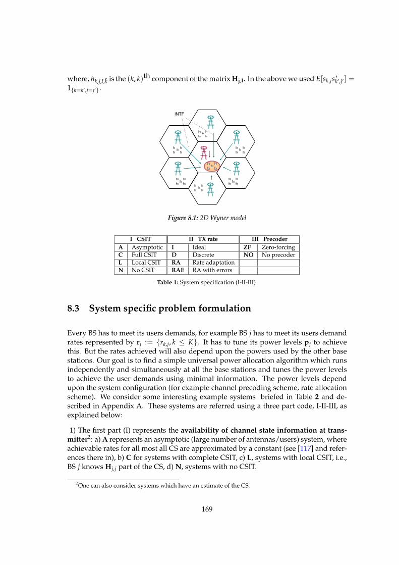
where, hk,j,l,k is the (k, k)th component of the matrix Hj,l. In the above we used E[sk,js∗k′,j′ ] =

1k=k′,j=j′.

Figure 8.1: 2D Wyner model

I CSIT II TX rate III PrecoderA Asymptotic I Ideal ZF Zero-forcingC Full CSIT D Discrete NO No precoderL Local CSIT RA Rate adaptationN No CSIT RAE RA with errors

Table 1: System specification (I-II-III)

8.3 System specific problem formulation

Every BS has to meet its users demands, for example BS j has to meet its users demandrates represented by rj := rk,j, k ≤ K. It has to tune its power levels pj to achievethis. But the rates achieved will also depend upon the powers used by the other basestations. Our goal is to find a simple universal power allocation algorithm which runsindependently and simultaneously at all the base stations and tunes the power levelsto achieve the user demands using minimal information. The power levels dependupon the system configuration (for example channel precoding scheme, rate allocationscheme). We consider some interesting example systems briefed in Table 2 and de-scribed in Appendix A. These systems are referred using a three part code, I-II-III, asexplained below:

1) The first part (I) represents the availability of channel state information at trans-mitter2: a) A represents an asymptotic (large number of antennas/users) system, whereachievable rates for all most all CS are approximated by a constant (see [117] and refer-ences there in), b) C for systems with complete CSIT, c) L, systems with local CSIT, i.e.,BS j knows Hj,j part of the CS, d) N, systems with no CSIT.

2One can also consider systems which have an estimate of the CS.

169

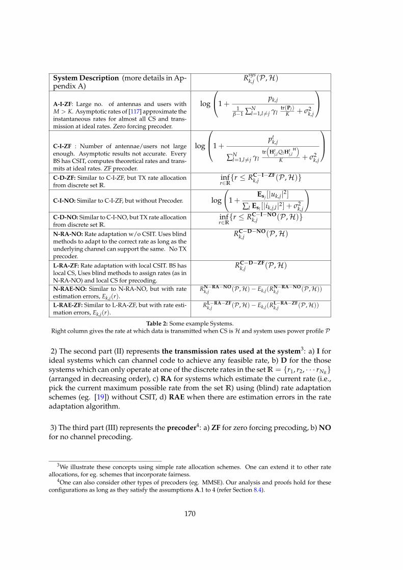
System Description (more details in Ap-pendix A)

Rsysk,j (P ,H)

A-I-ZF: Large no. of antennas and users withM > K. Asymptotic rates of [117] approximate theinstantaneous rates for almost all CS and trans-mission at ideal rates. Zero forcing precoder.

log

1 +pk,j

1β−1 ∑

Nl=1,l 6=j γl

tr(Pl)K + σ2

k,j

C-I-ZF : Number of antennae/users not largeenough. Asymptotic results not accurate. EveryBS has CSIT, computes theoretical rates and trans-mits at ideal rates. ZF precoder.

log

1 +

ptk,j

∑Nl=1,l 6=j γl

tr(

Htj,l QlHt

j,lH)

K + σ2k,j

C-D-ZF: Similar to C-I-ZF, but TX rate allocationfrom discrete set R.

infr∈R

r ≤ RC−I−ZFk,j (P ,H)

C-I-NO: Similar to C-I-ZF, but without Precoder. log

(

1 +Esj

[|uk,j|2]∑l Esl

[|ik,j,l |2] + σ2k,j

)

C-D-NO: Similar to C-I-NO, but TX rate allocationfrom discrete set R.

infr∈R

r ≤ RC−I−NOk,j (P ,H)

N-RA-NO: Rate adaptation w/o CSIT. Uses blindmethods to adapt to the correct rate as long as theunderlying channel can support the same. No TXprecoder.

RC−D−NOk,j (P ,H)

L-RA-ZF: Rate adaptation with local CSIT. BS haslocal CS, Uses blind methods to assign rates (as inN-RA-NO) and local CS for precoding.

RC−D−ZFk,j (P ,H)

N-RAE-NO: Similar to N-RA-NO, but with rateestimation errors, Ek,j(r).

RN−RA−NOk,j (P ,H)− Ek,j(RN−RA−NO

k,j (P ,H))

L-RAE-ZF: Similar to L-RA-ZF, but with rate esti-mation errors, Ek,j(r).

RL−RA−ZFk,j (P ,H)− Ek,j(RL−RA−ZF

k,j (P ,H))

Table 2: Some example Systems.Right column gives the rate at which data is transmitted when CS is H and system uses power profile P

2) The second part (II) represents the transmission rates used at the system3: a) I forideal systems which can channel code to achieve any feasible rate, b) D for the thosesystems which can only operate at one of the discrete rates in the set R = r1, r2, · · · rNR

(arranged in decreasing order), c) RA for systems which estimate the current rate (i.e.,pick the current maximum possible rate from the set R) using (blind) rate adaptationschemes (eg. [19]) without CSIT, d) RAE when there are estimation errors in the rateadaptation algorithm.

3) The third part (III) represents the precoder4: a) ZF for zero forcing precoding, b) NOfor no channel precoding.

3We illustrate these concepts using simple rate allocation schemes. One can extend it to other rateallocations, for eg. schemes that incorporate fairness.

4One can also consider other types of precoders (eg. MMSE). Our analysis and proofs hold for theseconfigurations as long as they satisfy the assumptions A.1 to 4 (refer Section 8.4).

170

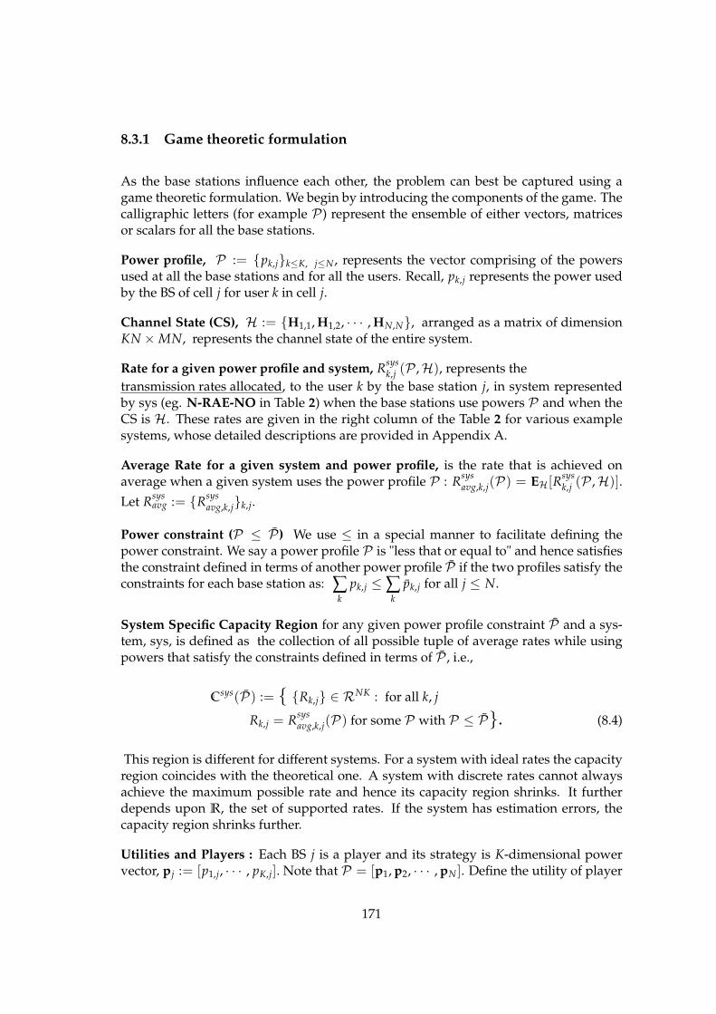
8.3.1 Game theoretic formulation

As the base stations influence each other, the problem can best be captured using agame theoretic formulation. We begin by introducing the components of the game. Thecalligraphic letters (for example P) represent the ensemble of either vectors, matricesor scalars for all the base stations.

Power profile, P := pk,jk≤K, j≤N , represents the vector comprising of the powersused at all the base stations and for all the users. Recall, pk,j represents the power usedby the BS of cell j for user k in cell j.

Channel State (CS), H := H1,1, H1,2, · · · , HN,N, arranged as a matrix of dimensionKN × MN, represents the channel state of the entire system.

Rate for a given power profile and system, Rsysk,j (P ,H), represents the

transmission rates allocated, to the user k by the base station j, in system representedby sys (eg. N-RAE-NO in Table 2) when the base stations use powers P and when theCS is H. These rates are given in the right column of the Table 2 for various examplesystems, whose detailed descriptions are provided in Appendix A.

Average Rate for a given system and power profile, is the rate that is achieved onaverage when a given system uses the power profile P : R

sysavg,k,j(P) = EH[R

sysk,j (P ,H)].

Let Rsysavg := R

sysavg,k,jk,j.

Power constraint (P ≤ P) We use ≤ in a special manner to facilitate defining thepower constraint. We say a power profile P is "less that or equal to" and hence satisfiesthe constraint defined in terms of another power profile P if the two profiles satisfy theconstraints for each base station as: ∑

k

pk,j ≤ ∑k

pk,j for all j ≤ N.

System Specific Capacity Region for any given power profile constraint P and a sys-tem, sys, is defined as the collection of all possible tuple of average rates while usingpowers that satisfy the constraints defined in terms of P , i.e.,

Csys(P) := Rk,j ∈ RNK : for all k, j

Rk,j = Rsysavg,k,j(P) for some P with P ≤ P. (8.4)

This region is different for different systems. For a system with ideal rates the capacityregion coincides with the theoretical one. A system with discrete rates cannot alwaysachieve the maximum possible rate and hence its capacity region shrinks. It furtherdepends upon R, the set of supported rates. If the system has estimation errors, thecapacity region shrinks further.

Utilities and Players : Each BS j is a player and its strategy is K-dimensional powervector, pj := [p1,j, · · · , pK,j]. Note that P = [p1, p2, · · · , pN ]. Define the utility of player

171

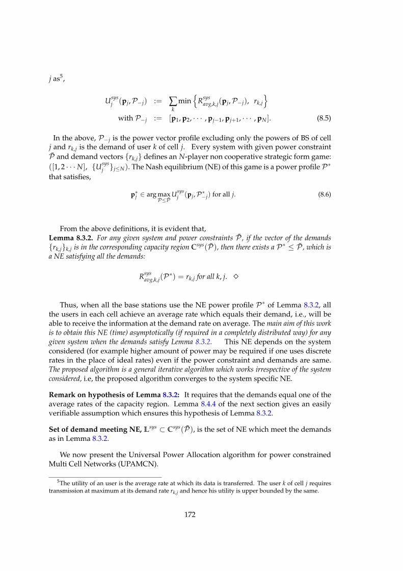
j as5,

Usysj (pj,P−j) := ∑

k

min

Rsysavg,k,j(pj,P−j), rk,j

with P−j := [p1, p2, · · · , pj−1, pj+1, · · · , pN ]. (8.5)

In the above, P−j is the power vector profile excluding only the powers of BS of cellj and rk,j is the demand of user k of cell j. Every system with given power constraintP and demand vectors rk,j defines an N-player non cooperative strategic form game:([1, 2 · · · N], U

sysj j≤N). The Nash equilibrium (NE) of this game is a power profile P∗

that satisfies,

p∗j ∈ arg max

P≤PU

sysj (pj,P∗

−j) for all j. (8.6)

From the above definitions, it is evident that,Lemma 8.3.2. For any given system and power constraints P , if the vector of the demandsrk,jk,j is in the corresponding capacity region C

sys(P), then there exists a P∗ ≤ P , which isa NE satisfying all the demands:

Rsysavg,k,j(P∗) = rk,j for all k, j. ⋄

Thus, when all the base stations use the NE power profile P∗ of Lemma 8.3.2, allthe users in each cell achieve an average rate which equals their demand, i.e., will beable to receive the information at the demand rate on average. The main aim of this workis to obtain this NE (time) asymptotically (if required in a completely distributed way) for anygiven system when the demands satisfy Lemma 8.3.2. This NE depends on the systemconsidered (for example higher amount of power may be required if one uses discreterates in the place of ideal rates) even if the power constraint and demands are same.The proposed algorithm is a general iterative algorithm which works irrespective of the systemconsidered, i.e, the proposed algorithm converges to the system specific NE.

Remark on hypothesis of Lemma 8.3.2: It requires that the demands equal one of theaverage rates of the capacity region. Lemma 8.4.4 of the next section gives an easilyverifiable assumption which ensures this hypothesis of Lemma 8.3.2.

Set of demand meeting NE, Lsys ⊂ C

sys(P), is the set of NE which meet the demandsas in Lemma 8.3.2.

We now present the Universal Power Allocation algorithm for power constrainedMulti Cell Networks (UPAMCN).

5The utility of an user is the average rate at which its data is transferred. The user k of cell j requirestransmission at maximum at its demand rate rk,j and hence his utility is upper bounded by the same.

172

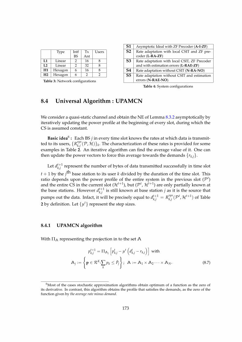
Type Intf Tx UsersBS Ant

L1 Linear 2 16 8L2 Linear 2 32 8H1 Hexagon 6 16 8H2 Hexagon 6 2 2

Table 3: Network configurations

S1 Asymptotic Ideal with ZF Precoder (A-I-ZF)S2 Rate adaptation with local CSIT and ZF pre-

coder (L-RA-ZF)S3 Rate adaptation with local CSIT, ZF Precoder

and with estimation errors (L-RAE-ZF)S4 Rate adaptation without CSIT (N-RA-NO)S5 Rate adaptation without CSIT and estimation

errors (N-RAE-NO).

Table 4: System configurations

8.4 Universal Algorithm : UPAMCN

We consider a quasi-static channel and obtain the NE of Lemma 8.3.2 asymptotically byiteratively updating the power profile at the beginning of every slot, during which theCS is assumed constant.

Basic idea6 : Each BS j in every time slot knows the rates at which data is transmit-ted to its users, R

sysk,j (P ,H)k. The characterization of these rates is provided for some

examples in Table 2. An iterative algorithm can find the average value of it. One canthen update the power vectors to force this average towards the demands rk,j.

Let dt+1k,j represent the number of bytes of data transmitted successfully in time slot

t + 1 by the jth base station to its user k divided by the duration of the time slot. Thisratio depends upon the power profile of the entire system in the previous slot (P t)and the entire CS in the current slot (Ht+1), but (P t, Ht+1) are only partially known atthe base stations. However dt+1

k,j is still known at base station j as it is the source that

pumps out the data. Infact, it will be precisely equal to dt+1k,j = R

sysk,j (P t,Ht+1) of Table

2 by definition. Let µt represent the step sizes.

8.4.1 UPAMCN algorithm

With ΠA representing the projection in to the set A

pt+1k,j = ΠAj

[

ptk,j − µt

(

dtk,j − rk,j

)]

with

Aj :=

p ∈ RK :∑k

pk ≤ Pj

; A := A1 × A2 · · · × AN . (8.7)

6Most of the cases stochastic approximation algorithms obtain optimum of a function as the zero ofits derivative. In contrast, this algorithm obtains the profile that satisfies the demands, as the zero of thefunction given by the average rate minus demand.

173

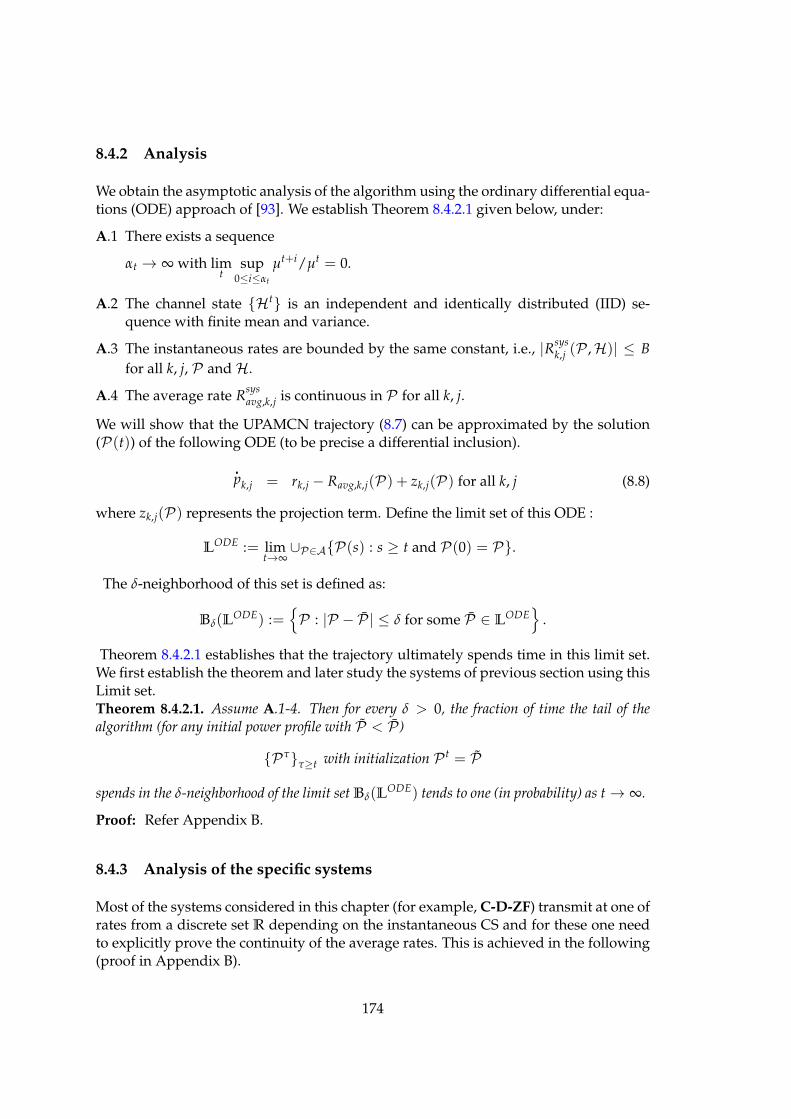
8.4.2 Analysis

We obtain the asymptotic analysis of the algorithm using the ordinary differential equa-tions (ODE) approach of [93]. We establish Theorem 8.4.2.1 given below, under:

A.1 There exists a sequence

αt → ∞ with limt

sup0≤i≤αt

µt+i/µt = 0.

A.2 The channel state Ht is an independent and identically distributed (IID) se-quence with finite mean and variance.

A.3 The instantaneous rates are bounded by the same constant, i.e., |Rsysk,j (P ,H)| ≤ B

for all k, j, P and H.

A.4 The average rate Rsysavg,k,j is continuous in P for all k, j.

We will show that the UPAMCN trajectory (8.7) can be approximated by the solution(P(t)) of the following ODE (to be precise a differential inclusion).

pk,j = rk,j − Ravg,k,j(P) + zk,j(P) for all k, j (8.8)

where zk,j(P) represents the projection term. Define the limit set of this ODE :

LODE := lim

t→∞∪P∈AP(s) : s ≥ t and P(0) = P.

The δ-neighborhood of this set is defined as:

Bδ(LODE) :=

P : |P − P| ≤ δ for some P ∈ LODE

.

Theorem 8.4.2.1 establishes that the trajectory ultimately spends time in this limit set.We first establish the theorem and later study the systems of previous section using thisLimit set.Theorem 8.4.2.1. Assume A.1-4. Then for every δ > 0, the fraction of time the tail of thealgorithm (for any initial power profile with P < P)

Pττ≥t with initialization P t = P

spends in the δ-neighborhood of the limit set Bδ(LODE) tends to one (in probability) as t → ∞.

Proof: Refer Appendix B.

8.4.3 Analysis of the specific systems

Most of the systems considered in this chapter (for example, C-D-ZF) transmit at one ofrates from a discrete set R depending on the instantaneous CS and for these one needto explicitly prove the continuity of the average rates. This is achieved in the following(proof in Appendix B).

174

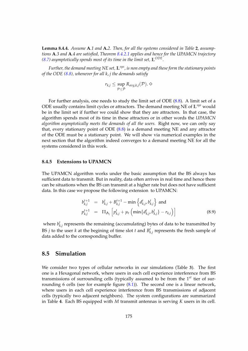
Lemma 8.4.4. Assume A.1 and A.2. Then, for all the systems considered in Table 2, assump-tions A.3 and A.4 are satisfied, Theorem 8.4.2.1 applies and hence for the UPAMCN trajectory(8.7) asymptotically spends most of its time in the limit set, L

ODE.

Further, the demand meeting NE set, Lsys, is non empty and these form the stationary points

of the ODE (8.8), whenever for all k, j the demands satisfy

rk,j ≤ supP≤P

Ravg,k,j(P). ⋄

For further analysis, one needs to study the limit set of ODE (8.8). A limit set of aODE usually contains limit cycles or attractors. The demand meeting NE of L

sys wouldbe in the limit set if further we could show that they are attractors. In that case, thealgorithm spends most of its time in these attractors or in other words the UPAMCNalgorithm asymptotically meets the demands of all the users. Right now, we can only saythat, every stationary point of ODE (8.8) is a demand meeting NE and any attractorof the ODE must be a stationary point. We will show via numerical examples in thenext section that the algorithm indeed converges to a demand meeting NE for all thesystems considered in this work.

8.4.5 Extensions to UPAMCN

The UPAMCN algorithm works under the basic assumption that the BS always hassufficient data to transmit. But in reality, data often arrives in real time and hence therecan be situations when the BS can transmit at a higher rate but does not have sufficientdata. In this case we propose the following extension to UPAMCN:

bt+1k,j = bt

k,j + Bt+1k,j − min

dtk,j, bt

k,j

and

pt+1k,j = ΠAj

[

ptk,j + µt

(

mindtk,j, bt

k,j − rk,j

)]

(8.9)

where btk,j represents the remaining (accumulating) bytes of data to be transmitted by

BS j to the user k at the begining of time slot t and Btk,j represents the fresh sample of

data added to the corresponding buffer.

8.5 Simulation

We consider two types of cellular networks in our simulations (Table 3). The firstone is a Hexagonal network, where users in each cell experience interference from BStransmissions of surrounding cells (typically assumed to be from the 1st tier of sur-rounding 6 cells (see for example figure (8.1)). The second one is a linear network,where users in each cell experience interference from BS transmissions of adjacentcells (typically two adjacent neighbors). The system configurations are summarizedin Table 4. Each BS equipped with M transmit antennas is serving K users in its cell.

175

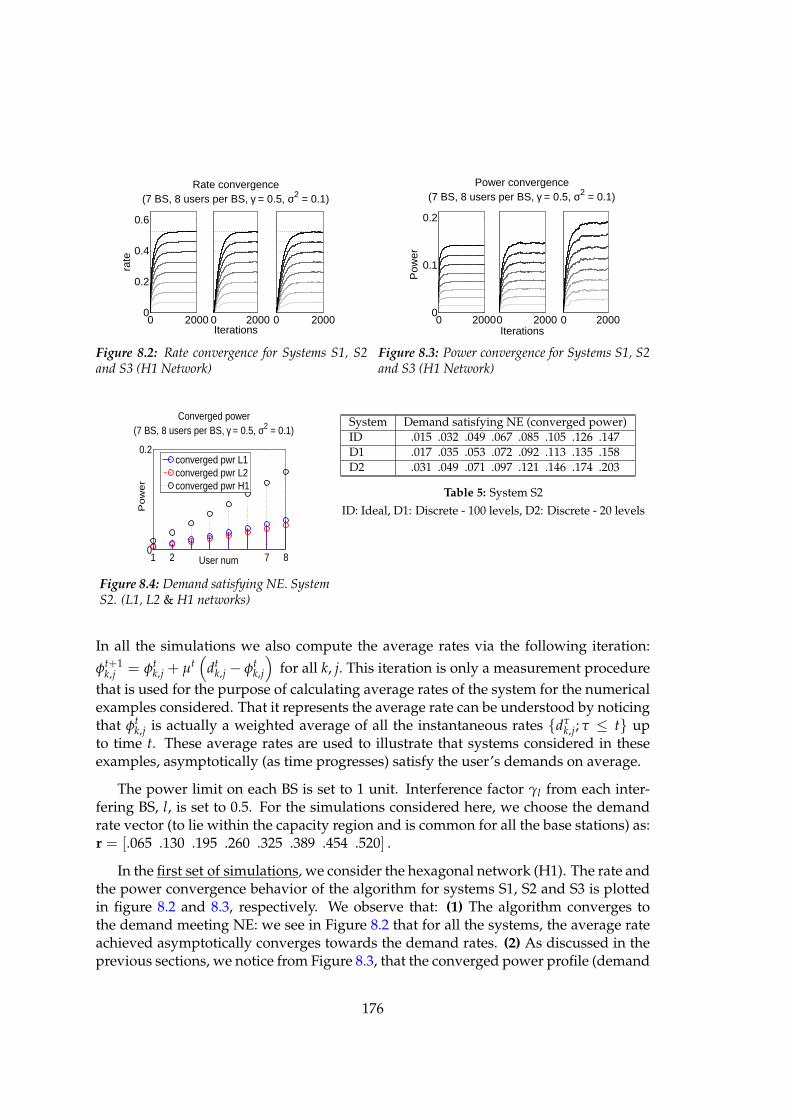
0 20000

0.2

0.4

0.6

rate

0 2000

Rate convergence(7 BS, 8 users per BS, γ = 0.5, σ2 = 0.1)

Iterations0 2000

Figure 8.2: Rate convergence for Systems S1, S2and S3 (H1 Network)

0 20000

0.1

0.2

Pow

er

0 2000

Power convergence(7 BS, 8 users per BS, γ = 0.5, σ2 = 0.1)

Iterations0 2000

Figure 8.3: Power convergence for Systems S1, S2and S3 (H1 Network)

1 2 7 80

0.2

User num

Po

we

r

Converged power(7 BS, 8 users per BS, γ = 0.5, σ2 = 0.1)

converged pwr L1converged pwr L2converged pwr H1

Figure 8.4: Demand satisfying NE. SystemS2. (L1, L2 & H1 networks)

System Demand satisfying NE (converged power)ID .015 .032 .049 .067 .085 .105 .126 .147D1 .017 .035 .053 .072 .092 .113 .135 .158D2 .031 .049 .071 .097 .121 .146 .174 .203

Table 5: System S2

ID: Ideal, D1: Discrete - 100 levels, D2: Discrete - 20 levels

In all the simulations we also compute the average rates via the following iteration:

φt+1k,j = φt

k,j + µt(

dtk,j − φt

k,j

)

for all k, j. This iteration is only a measurement procedurethat is used for the purpose of calculating average rates of the system for the numericalexamples considered. That it represents the average rate can be understood by noticingthat φt

k,j is actually a weighted average of all the instantaneous rates dτk,j; τ ≤ t up

to time t. These average rates are used to illustrate that systems considered in theseexamples, asymptotically (as time progresses) satisfy the user’s demands on average.

The power limit on each BS is set to 1 unit. Interference factor γl from each inter-fering BS, l, is set to 0.5. For the simulations considered here, we choose the demandrate vector (to lie within the capacity region and is common for all the base stations) as:r = [.065 .130 .195 .260 .325 .389 .454 .520] .

In the first set of simulations, we consider the hexagonal network (H1). The rate andthe power convergence behavior of the algorithm for systems S1, S2 and S3 is plottedin figure 8.2 and 8.3, respectively. We observe that: (1) The algorithm converges tothe demand meeting NE: we see in Figure 8.2 that for all the systems, the average rateachieved asymptotically converges towards the demand rates. (2) As discussed in theprevious sections, we notice from Figure 8.3, that the converged power profile (demand

176

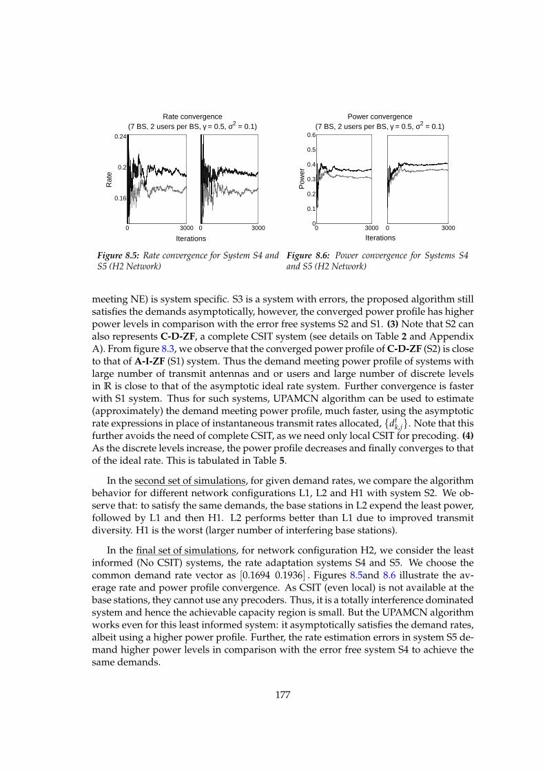
0 3000

0.16

0.2

0.24

Rat

eRate convergence

(7 BS, 2 users per BS, γ = 0.5, σ2 = 0.1)

0 3000

Iterations

Figure 8.5: Rate convergence for System S4 andS5 (H2 Network)

0 30000

0.1

0.2

0.3

0.4

0.5

0.6

Pow

er

Power convergence(7 BS, 2 users per BS, γ = 0.5, σ2 = 0.1)

0 3000

Iterations

Figure 8.6: Power convergence for Systems S4and S5 (H2 Network)

meeting NE) is system specific. S3 is a system with errors, the proposed algorithm stillsatisfies the demands asymptotically, however, the converged power profile has higherpower levels in comparison with the error free systems S2 and S1. (3) Note that S2 canalso represents C-D-ZF, a complete CSIT system (see details on Table 2 and AppendixA). From figure 8.3, we observe that the converged power profile of C-D-ZF (S2) is closeto that of A-I-ZF (S1) system. Thus the demand meeting power profile of systems withlarge number of transmit antennas and or users and large number of discrete levelsin R is close to that of the asymptotic ideal rate system. Further convergence is fasterwith S1 system. Thus for such systems, UPAMCN algorithm can be used to estimate(approximately) the demand meeting power profile, much faster, using the asymptoticrate expressions in place of instantaneous transmit rates allocated, dt

k,j. Note that thisfurther avoids the need of complete CSIT, as we need only local CSIT for precoding. (4)As the discrete levels increase, the power profile decreases and finally converges to thatof the ideal rate. This is tabulated in Table 5.

In the second set of simulations, for given demand rates, we compare the algorithmbehavior for different network configurations L1, L2 and H1 with system S2. We ob-serve that: to satisfy the same demands, the base stations in L2 expend the least power,followed by L1 and then H1. L2 performs better than L1 due to improved transmitdiversity. H1 is the worst (larger number of interfering base stations).

In the final set of simulations, for network configuration H2, we consider the leastinformed (No CSIT) systems, the rate adaptation systems S4 and S5. We choose thecommon demand rate vector as [0.1694 0.1936] . Figures 8.5and 8.6 illustrate the av-erage rate and power profile convergence. As CSIT (even local) is not available at thebase stations, they cannot use any precoders. Thus, it is a totally interference dominatedsystem and hence the achievable capacity region is small. But the UPAMCN algorithmworks even for this least informed system: it asymptotically satisfies the demand rates,albeit using a higher power profile. Further, the rate estimation errors in system S5 de-mand higher power levels in comparison with the error free system S4 to achieve thesame demands.

177

Further, we observe that the convergence to the demand meeting NE is quicker inthose systems where base stations have more information (see for eg. figure 8.3).

8.6 Conclusions

Mobile broadband users demand certain rates depending on the end application andQoS requirements. The base station serving these users has to allocate power to satisfyuser demands operating within its own total power budget. Intra-cell and inter-cellinterference diminish the available rates in multicell networks. Neighboring base sta-tions can co-operate to exchange some form of channel state information dependingon backhaul capacity and processing power to alleviate interference and thus enhanceachievable rates. Further, system specific components like modulation, coding, rateallocation, channel estimation and synchronization impacts the achievable rates andhence the power allocation. In our work, we propose an universal power allocationalgorithm which works in this setting. The stochastic approximation based univer-sal power allocation algorithm runs at each BS, independently and simultaneously tomeet the user demands as long as the demands are achievable. The power allocationis formulated as a game problem. A system specific capacity region is defined andthe proposed algorithm is analyzed with an ODE framework. The proposed algorithmworks well in a multitude of system configurations as demonstrated via simulationsand analysis.

Our algorithm assumes that the serving BS always has sufficient amount of datato transmit. However, in many applications, the data is available in real time. Wementioned a possible extension of the same in the work.

8.7 Appendix A: Example Systems

1) Asymptotic Ideal Rate system : In a multicellular system with large number of antennasat the BS and large number of users, the rate for a given CS can be obtained usingrandom matrix theory. For example, in [117] the asymptotic rates are derived for a zeroforcing (ZF) precoder. It is shown that for almost all realizations of CS, the rate can beapproximated by the expression given below in equation (8.10). Further, we consider asystem in which, the base stations use channel coding schemes to transmit very closeto the theoretical rates. When this system (which we call as asym-ideal-zeroforcing or inshort A-I-ZF according to our notations) uses power profile P and when the channelstate (CS) is H, the BS j transmits to the user k at rate ([117]) (when M > K):

RA−I−ZFk,j (P ,H) ≈ log

1+pk,j

1β−1 ∑

Nl=1,l 6=j γl

tr(Pl)K + σ2

k,j

(8.10)

where, β = M/K is the ratio of number of transmit antennas on the BS to the numberof users and γl ∈ (0, 1) represents the interference from cell l. This rate is same for

178

almost all CS H as it is an asymptotic rate. Similar expression is available for the casewith M = K in [117].

2) Ideal rates using complete CSIT : If the number of antennae/number of users is not largeenough, the asymptotic results are not accurate. If BS has access to CSIT (and if eachBS could channel code to obtain rates closer to the ideal rate) then with ZF precoder ittransmits at rate:

RC−I−ZFk,j (P ,H) = log

1 +pt

k,j

∑Nl=1,l 6=j γl

tr(

Htj,l Ql Ht

j,lH)

K + σ2k,j

Ql := HtlH(Ht

l HtlH)−1Pt

l(Htl H

tlH)−1Ht

l

For the same configuration, but without transmitter precoding, the the instantaneoustransmission rate (as obtained using Shannon’s capacity expression), from equation(8.2) is:

RC−I−NOk,j (P ,H) = log(1 + ηk,j) where (8.11)

SINR, ηk,j :=E[|uk,j|2]

ρk,jwith noise + interference, ρk,j := ∑

l

E[|ik,j,l |2] + σ2k,j.

3) Finite number of Rates : Ideal rate systems are not realistic, they can’t be implementedin practice. We consider a system, in which the BS can transmit at one of the availablediscrete rates from the set R. When transmitter has CSIT, it knows the exact theoreticalrate and hence will pick the largest rate from set R that is smaller than the currenttheoretical rate:

RC−D−ZFk,j (P ,H) = inf

r∈R

r ≤ RC−I−ZFk,j (P ,H), (8.12)

RC−D−NOk,j (P ,H) = inf

r∈R

r ≤ RC−I−NOk,j (P ,H). (8.13)

4) Rate adaptation Without CSIT : It is once again not realistic to assume the knowl-edge of complete CSIT. There are many schemes that estimate the rate blindly or usingsome partial CSIT (eg. [19]). The UPAMCN algorithm is a very general algorithm andworks with all those systems which satisfy assumptions A.1-4. These are quite simpleassumptions and most of the systems can satisfy these and hence the algorithm worksfor majority of the blind/partial CSIT systems.

We explain one such blind system wherein, the BS estimates the transmission rateswithout knowledge of CSIT. Each time, the BS begins by attempting at the highest avail-able rate r1. If the data is not received correctly (information obtained via a feedbackfrom the receiver), the BS sends some more information about the same data packetso that the overall rate now is the second highest r2. This procedure repeats until thetwo agree upon the correct rate. We assume that this rate adaptation system is alwayssuccessful, i.e, it can estimate the actual rates without errors. Such a system does not re-quire CSIT, however the final rate at which the transmission takes place depends uponthe current channel state in exactly the same way as in the case of C-D (or A-D for largeantenna and user case and note there is no channel coding in this case as there is noCSIT) and hence,

RN−RA−NOk,j (P ,H) = RC−D−NO

k,j (P ,H) (8.14)

179

5) Rate Adaptation with local CSIT: All the base stations have local CSIT, i.e., BS j knowsthe Hj,j part of CS. However they can’t estimate the current rates just based on localCSIT. So, they once again use rate adaptation technique as in the system (4). They canhowever design a better system by using for example a zero forcing precoder. In thiscase, as in system (4) the rate will be adapted to the actual underlying rate and hencewill be same as that in C-D-ZF:

RL−RA−ZF(P ,H) = RC−D−ZFk,j (P ,H) (8.15)

6) Rate Adaptation with errors : There can be some errors in rate adaptation algorithmof system (4) or (5). In this case

RN−RAE−NOk,j (P ,H)

= RN−RA−NOk,j (P ,H)− Ek,j(RN−RA−NO

k,j (P ,H)) (8.16)

RL−RAE−ZFk,j (P ,H)

= RL−RA−ZFk,j (P ,H)− Ek,j(RL−RA−ZF

k,j (P ,H)) (8.17)

where (assuming independent errors) Ek,j(r) can take values in the subset R ∩ r ≤ rwith a given probability distribution.

8.8 Appendix B: Proofs

Proof of Theorem 1: As a first step, we rewrite the algorithm as in [93]:

Ytk,j := rk,j − dt

k,j, pt+1k,j = ΠAj

[

ptk,j + µtYt

k,j

]

.

Define, Ft := σ(

Pτ, Yτ−1k,j k,j, for all τ ≤ t

)

and let Et represent the expectation w.r.t.Ft, the filtration. Under the assumptions A.2 and A.3 clearly the condition expectation

Et[Ytk,j] = g

pk,j(P t) := rk,j − Ravg,k,j(P t)for all k, j and t.

For every j, the constrain set Aj satisfies the assumption (A3.2), page 107 of [93]. Byassumption A.3 Yt

k,j; t is uniformly integrable and hence satisfies assumption A.2.1,pp. 258 [93]. They also satisfy the assumption A.2.3 to A.2.7 of pages 258, 259 [93] withgt = g = gp and with βt = 0 ξt = 0 for all time t. Assumption A.2.2, pp 258, [93] issatisfied because of our Assumption A.4. Let zj represent the projection or constraintterm, the minimum force needed to keep the vector pj in Aj. Then by Theorem 2.3,pp. 259, [93] the UPAMCN algorithm trajectory P t converges weekly to the trajectoryof the solution of the ODE (8.8) (in the sense as explained in [93]). Further by the sametheorem of [93], for any δ > 0, the fraction of time that the tail sequence Pττ≥t, withinitializations pt

k,j = pk,j for every (k, j), spends in the δ-neighborhood of the limit of set

of the above ODE (8.8), Bδ(LODE), goes to one (in probability) as t → ∞. ⋄

180

Proof of Lemma 8.4.4: The boundedness assumption A.3 is direct for discrete ratesystems and is also true for ideal rate systems as seen from the formulas. The idealrates are point wise continuous and are bounded and hence by bounded convergencetheorem satisfy the continuous assumption A.4. The same for the discrete rates is givenby Lemma 8.8.1.

The continuity assumption A.4 now also holds for the rate adaptation system with er-rors, L-RAE-NO, whenever the statistics of the errors Ek,j are independent of thepower profile or when they are continuous in P . Thus for all the systems considered in thiswork Theorem 8.4.2.1 applies.

Conditions for existence of demand meeting NE : For all the systems considered sofar, the hypothesis of Lemma 8.3.2 is satisfied, i.e., L

NE is non empty whenever thepower constraints are sufficient to cater to the demand rates. This fact is established bythe continuity of the average rates w.r.t. the power profile, i.e., the establishment of theassumption A.4. To be precise Lemma 8.3.2 is satisfied, i.e., L

NE is non empty whenever forall k, j rk,j ≤ sup

P≤PRavg,k,j(P). ⋄

Lemma 8.8.1. The average rates Rsysavg,k,j for systems C-D-ZF and C-D-NO are continuous

w.r.t. power profile P for all k, j.

Proof : Let Rk,j(P ,H) represent the corresponding ideal rate (the rate before dis-cretization) for the given CS H. From all the rate formulas in this work, we can see thatthese rates bounded and are continuous in P , for all H. For the discretized systems, theaverage rates can be written as,

Ravg,k,j(P) = ∑i≤N

q(i,P)ri where

q(i,P) :=∫

1ri−1≤Rk,j(P ,H)≤ridΓ(H) (8.18)

with dΓ representing the Gaussian measure. For a given P , the probability of the setsof the type (the boundaries of the sets used while defining the indicators in (8.18))

Γ(

H : Rk,j(P ,H) = ri

)

= 0,

because of the continuity of the Gaussian measure. Hence, the point wise functions ofintegral (8.18) are continuous w.r.t. to P for almost all H. Thus the lemma follows bybounded convergence theorem. ⋄

8.9 Publications

1. Sreenath Ramanath, Veeraruna Kavitha, Merouane Debbah, "Satisfying Demandsin a Multicellular Network: An Universal Power Allocation Algorithm", proceed-ings of WiOpt 2011, May 9-13, Princeton, USA.

181

Part IV

Epilogue

183

Chapter 9

Conclusions

Summary and general discussion

Small cell networks are a promising alternative to increasing data demands arising dueto new applications and services in mobile broadband. Optimal design of small cells isa challenging task. In this thesis we addressed two important aspects of small cells: celldimensioning and resource allocation.

We began our discussion with dimensioning of static and moving users. For the caseof static users, in chapter 2, we used fluid limits to derive explicit expressions for owncell and interference power and computed throughput achievable as a function of cellsize. Our analysis considered frequency reuse, path-loss, different receiver structures,indoor-outdoor partitions, etc. Our results showed that optimal cell sizes exist in someconfigurations, while in the others, the way to maximize achievable throughput was toincrease the base station density. A scope for future directions is to consider more so-phisticated radio propagation models, fading and shadowing effects, etc. Further, fluidmodels were used to get first-cut results for cell dimensioning, but one can consider amore closer to realistic situations, like the users are distributed according to a stochasticprocess and thus meaningful results can be obtained using tools like stochastic geome-try [17].

For the case of mobile users, in chapter 3, we used queuing theoretic tools to de-rive optimal cell sizes which optimize important system metrics like expected wait-ing/service times, call drop/block probabilities, etc. Our analysis was predominantlyfor users traversing in single dimensions and further once a velocity is chosen by a cer-tain user, it is assumed that the user continues with the same velocity until his serviceis completed or until the time he is blocked or dropped. Many interesting possibili-ties exist as scope towards future research. Some of these have been mentioned in ourwork [89]. Extensions would include analysis in 2-dimensions and further assumingthat users travel with a velocity with a certain mean and variance. We have carried outpartial analysis of some of these in our work [118]. Further, it would be interesting toconsider more sophisticated and realistic user movements which can be modeled by

185

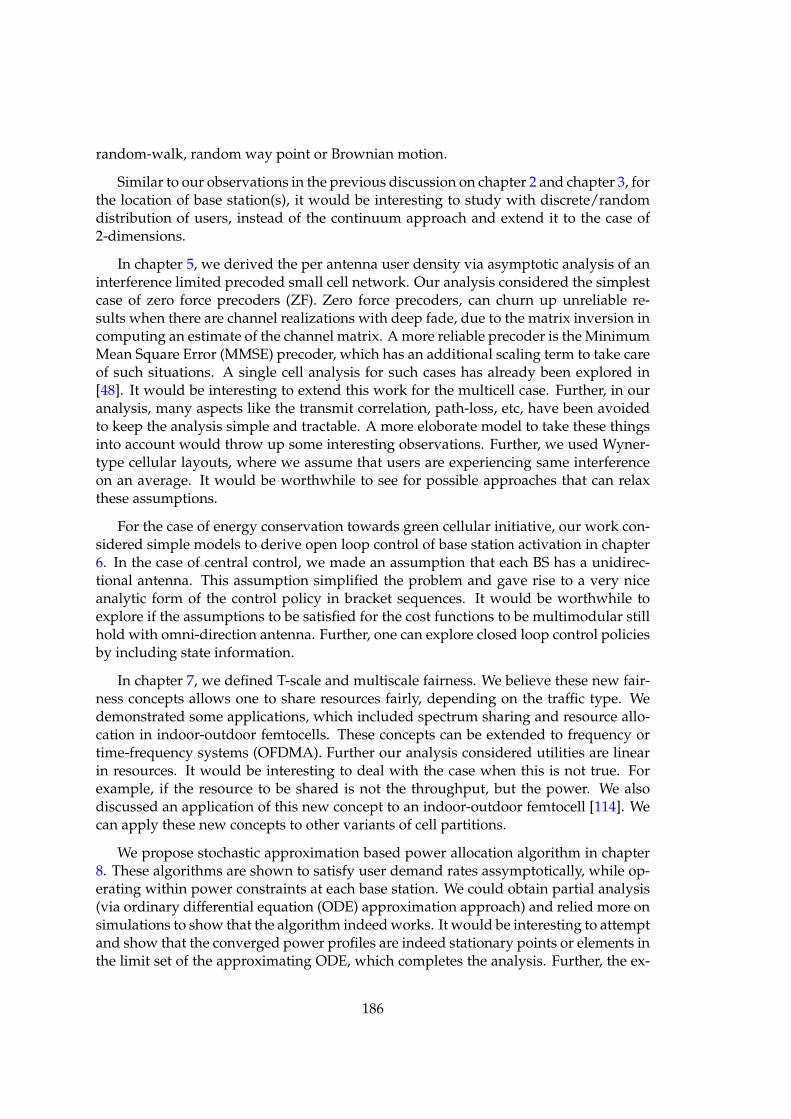
random-walk, random way point or Brownian motion.

Similar to our observations in the previous discussion on chapter 2 and chapter 3, forthe location of base station(s), it would be interesting to study with discrete/randomdistribution of users, instead of the continuum approach and extend it to the case of2-dimensions.

In chapter 5, we derived the per antenna user density via asymptotic analysis of aninterference limited precoded small cell network. Our analysis considered the simplestcase of zero force precoders (ZF). Zero force precoders, can churn up unreliable re-sults when there are channel realizations with deep fade, due to the matrix inversion incomputing an estimate of the channel matrix. A more reliable precoder is the MinimumMean Square Error (MMSE) precoder, which has an additional scaling term to take careof such situations. A single cell analysis for such cases has already been explored in[48]. It would be interesting to extend this work for the multicell case. Further, in ouranalysis, many aspects like the transmit correlation, path-loss, etc, have been avoidedto keep the analysis simple and tractable. A more eloborate model to take these thingsinto account would throw up some interesting observations. Further, we used Wyner-type cellular layouts, where we assume that users are experiencing same interferenceon an average. It would be worthwhile to see for possible approaches that can relaxthese assumptions.

For the case of energy conservation towards green cellular initiative, our work con-sidered simple models to derive open loop control of base station activation in chapter6. In the case of central control, we made an assumption that each BS has a unidirec-tional antenna. This assumption simplified the problem and gave rise to a very niceanalytic form of the control policy in bracket sequences. It would be worthwhile toexplore if the assumptions to be satisfied for the cost functions to be multimodular stillhold with omni-direction antenna. Further, one can explore closed loop control policiesby including state information.

In chapter 7, we defined T-scale and multiscale fairness. We believe these new fair-ness concepts allows one to share resources fairly, depending on the traffic type. Wedemonstrated some applications, which included spectrum sharing and resource allo-cation in indoor-outdoor femtocells. These concepts can be extended to frequency ortime-frequency systems (OFDMA). Further our analysis considered utilities are linearin resources. It would be interesting to deal with the case when this is not true. Forexample, if the resource to be shared is not the throughput, but the power. We alsodiscussed an application of this new concept to an indoor-outdoor femtocell [114]. Wecan apply these new concepts to other variants of cell partitions.

We propose stochastic approximation based power allocation algorithm in chapter8. These algorithms are shown to satisfy user demand rates assymptotically, while op-erating within power constraints at each base station. We could obtain partial analysis(via ordinary differential equation (ODE) approximation approach) and relied more onsimulations to show that the algorithm indeed works. It would be interesting to attemptand show that the converged power profiles are indeed stationary points or elements inthe limit set of the approximating ODE, which completes the analysis. Further, the ex-

186

tension to multi-tier and heterogeneous networks, considering this algorithm is againdemonstrated via simulations. It would be challenging to analyze this problem viasome sort of two-time scale stochastic approximation based analysis (e.g., see [32]).

Finally, some of the ideas developed during the process of study should find use inpractical implementation of small cell networks. It would be of great value to demon-strate few key ideas used in cell dimensioning and resource allocation on a more com-prehensive evaluation platform, like an LTE simulator [161].

187

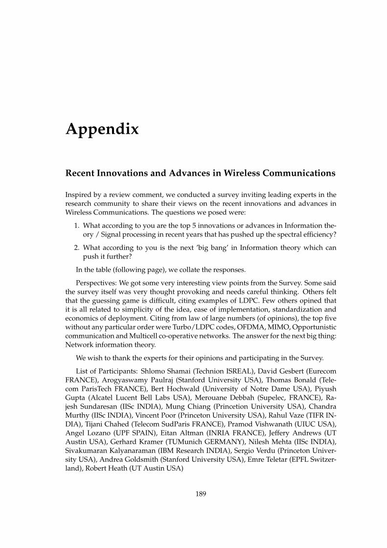
Appendix

Recent Innovations and Advances in Wireless Communications

Inspired by a review comment, we conducted a survey inviting leading experts in theresearch community to share their views on the recent innovations and advances inWireless Communications. The questions we posed were:

1. What according to you are the top 5 innovations or advances in Information the-ory / Signal processing in recent years that has pushed up the spectral efficiency?

2. What according to you is the next ’big bang’ in Information theory which canpush it further?

In the table (following page), we collate the responses.

Perspectives: We got some very interesting view points from the Survey. Some saidthe survey itself was very thought provoking and needs careful thinking. Others feltthat the guessing game is difficult, citing examples of LDPC. Few others opined thatit is all related to simplicity of the idea, ease of implementation, standardization andeconomics of deployment. Citing from law of large numbers (of opinions), the top fivewithout any particular order were Turbo/LDPC codes, OFDMA, MIMO, Opportunisticcommunication and Multicell co-operative networks. The answer for the next big thing:Network information theory.

We wish to thank the experts for their opinions and participating in the Survey.

List of Participants: Shlomo Shamai (Technion ISREAL), David Gesbert (EurecomFRANCE), Arogyaswamy Paulraj (Stanford University USA), Thomas Bonald (Tele-com ParisTech FRANCE), Bert Hochwald (University of Notre Dame USA), PiyushGupta (Alcatel Lucent Bell Labs USA), Merouane Debbah (Supelec, FRANCE), Ra-jesh Sundaresan (IISc INDIA), Mung Chiang (Princetion University USA), ChandraMurthy (IISc INDIA), Vincent Poor (Princeton University USA), Rahul Vaze (TIFR IN-DIA), Tijani Chahed (Telecom SudParis FRANCE), Pramod Vishwanath (UIUC USA),Angel Lozano (UPF SPAIN), Eitan Altman (INRIA FRANCE), Jeffery Andrews (UTAustin USA), Gerhard Kramer (TUMunich GERMANY), Nilesh Mehta (IISc INDIA),Sivakumaran Kalyanaraman (IBM Research INDIA), Sergio Verdu (Princeton Univer-sity USA), Andrea Goldsmith (Stanford University USA), Emre Teletar (EPFL Switzer-land), Robert Heath (UT Austin USA)

189

!" # $%

• &&'

•

• #

• & (

• '% &#

)*+ &&' )*,**- &&'./ *

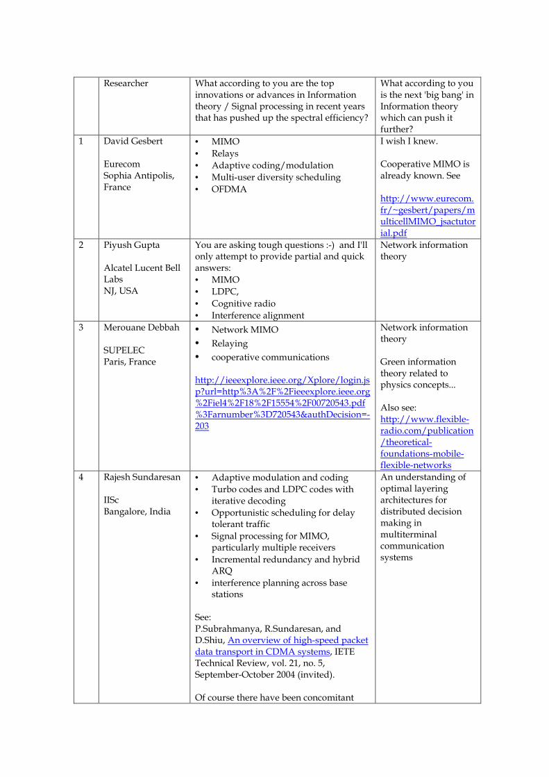
0 1 !#23245$6#

7) 8 ,(9 8 ),

• &&'

• 2 1+$

• +

•

4)

: & 61"2"+1 $%

• 4)&&'

•

• , * *; */<=:#=0%=0% * *=0% >=0%?=0%@@@>=0%AAB0A@>:*=:%=: B0A@>:C <(0A:

4) ! ***#,,* ( * ( ( ( ()

> /3$

• #

• D2 1+

• '

• &&'$

• #E

•

,1*$*$ * $# () + &#$"D"D $*0$*@$('0AA>F 9*'

# )

G28 *

@ " #4# # $%

• D)

• + +)3 1

• ( (

H D I $

• FD(2 1+9 *

• '$ ( F) J9$ K F@ 9$ $ $ *

#$ $8 *4 $ D *4 F 2 1+ ! 9 /$ $ *

B 5#6D# 6#

D) (8 *D ) $ ) * *L+AAAL) *

? #2K61%3$

1I7, * *.*/<@B>HA

M D3D1 D%

• D2 1+

• '

• # C

• &&'

• '% &#

A 1G D8 *

66+6$2$6#

F L)( L$ $ $ F 99 ) * 8 ) )

GKD%& $4 #

I7*9D@*9 )9+ &&'9# F 99D 'F* $N 99& %F390943 ,9N $4) D *

0 3I6 4 $6#

/$ (( &&'*D 2 1+$ + (03$&&' *') $ '% &# (F+ &#D &#9 $ &2D"*D $ ) *

: # *1/6 $6#

,*0A* * <H0

> G 11 6 $6#

D) $O ) $ , *D &&'$ $*

@ &+ 1 6 $6#

) $*#) $*)0A8*

H +3$4 #

D 8 J )()J

B !PD6& $!"&#47

) $ *

Index

T-scale fairness, 150α-fair assignment, 147α-fairness, 93, 148α-fairness instantaneous, 149α-fairness long term, 149

Arrivals, 68Asymptotic, 118, 135Attenuation, 53

Block probability, 66, 77, 83Bracket sequence, 133BS location-indoor, 53BS location-outdoor, 54BS placement, 91, 95, 96, 110

Centralized control, 134Channel inversion precoding, 117Coefficient of variation, 160Conservation factor, 134

Decentralized control, 136Drop probability, 66, 77, 84, 89

Elastic calls, 75Ergodic capacity, 118

Fairness instantaneous, 156, 161Fairness longterm, 157, 162Fairness midterm, 156Fairness multiscale, 158Fairness parameter, 92Fast BS switching, 65Fluid model, 50

Gilbert channel, 155

Handover, 68Handover distribution, 88Handover macrocell, 73

Handover rate, 73Handover smallcell, 82Handover speed distribution, 83Hexagonal grid, 55

Indoor-outdoor, 160

Large population limits, 92, 93, 110Limit Velocity, 72

Max-min fairness, 93MIMO, 113Moments of service time, 74, 86Multimodularity, 133Multiscale fairness, 152

Non-elastic calls, 77

Open loop, 132Optimal cell size, 52, 74Outdoor cell, 99

Path loss, 69Policy, 132Power allocation, 172Power constraint, 117Precoding matrix, 117Proportional fairness, 93

Radio conditions, 69Random matrix theory, 115Resource allocation, 145

Service time, 66, 73, 81Spatial queuing, 66Split cell, 102Stability factor, 83, 89Stieltjes transform, 115Stochastic approximation, 173Street grid, 78

193

Sum rate, 118System specific capacity region, 166, 171

Throughput density, 57Traffic types, 68

Utility, 148, 171

Virtual Cell, 65

Waiting time, 66, 75Wyner, 115

ZF precoding, 117

194

Publications

JOURNALS

1. Veeraruna Kavitha, Sreenath Ramanath and Eitan Altman, "Spatial queuing anal-ysis for design and dimensioning of Picocell networks with mobile users", Else-viers Performance Evaluation, Volume 68, Issue 8.

CONFERENCES AND WORKSHOPS

1. Sreenath Ramanath, Veeraruna Kavitha, Eitan Altman, "Open Loop Optimal Con-trol of Base Station Activation for Green Networks", proceedings of WiOpt 2011,May 9-13, Princeton, USA.

2. Sreenath Ramanath, Veeraruna Kavitha, Merouane Debbah, "Satisfying Demandsin a Multicellular Network: An Universal Power Allocation Algorithm", proceed-ings of WiOpt 2011, May 9-13, Princeton, USA.

3. Sreenath Ramanath, Eitan Altman, Konstantin Avrachenkov, "A heterogeneousapproach to fair resource allocation and its application in femtocell networks",proceedings of the Workshop on Indoor and Outdoor Femto Cells (IOFC’11), May13, Princeton USA.

4. Eitan Altman, Konstantin Avrachenkov, Sreenath Ramanath, "Multiscale Fairnessand its Application to Resource Allocation in Wireless Networks", proceedings ofIFIP Networking 2011, LNCS 6631, May 9-13, Valencia, Spain.

5. Eitan Altman, Konstantin Avrachenkov, Sreenath Ramanath, "Multiscale Fairnessand its Networking Application", Poster, Performance 2010, Nov 17-19, Namur,Belgium.

6. Sreenath Ramanath, Veeraruna Kavitha, Eitan Altman, "Impact of mobility oncall block, call drops and optimal cell size in small cell networks", proceedings ofthe Workshop on Indoor and Outdoor Femto Cells (IOFC’10), Sep 26, Istanbul,Turkey.

7. Sreenath Ramanath, Veeraruna Kavitha, Eitan Altman, "Spatial queuing analysisfor mobility in pico cell networks", proceedings of WiOpt 2010, May 31-Jun 04,Avignon, France.

195

8. Sreenath Ramanath, Merouane Debbah, Eitan Altman, Vinod Kumar, "Asymp-totic analysis of precoded small cell networks", proceedings of InfoCom 2010, Mar15-19, San Diego, USA.

9. Sreenath Ramanath, Eitan Altman, Vinod Kumar, Merouane Debbah, "Optimiz-ing cell size in pico-cell networks", Invited paper, Workshop on Resource Alloca-tion in Wireless Networks (RAWNET’09), Jun 27, Seoul, South Korea.

10. Sreenath Ramanath, Eitan Altman, Vinod Kumar, Veeraruna Kavitha, LaurentThomas, "Fair assignment of base stations in cellular networks", proceedings ofthe 22nd World Wireless Research Forum (WWRF’09), May 5-7, Paris, France.

TECHNICAL REPORTS

1. Eitan Altman, Konstantin Avrachenkov and Sreenath Ramanath, "Multiscale Fair-ness and its Application to Dynamic Resource Allocation in Wireless Networks",INRIA research report number RR-7382 available at http://hal.inria.fr/inria-00515430/en/

196

Bibliography

[1] Robert. A, Dinesh. T, and Xinrong. Li. Indoor propogation modeling at 2.4 ghzfor 1eee 802.11 networks. In Proceedings of the International conference on wirelessand optical communication, Jul 2006.

[2] N. Abramson. The aloha system - another alternative for computer communica-tions. In Proceedings of the Fall Joint Computer Conference, 1970.

[3] S. M. Alamouti. A simple transmit diversity technique for wireless communica-tions. IEEE JSAC, 16:1451–1458, 1998.

[4] Alcatel-Lucent. Beyond the base station router. technical note.

[5] E. Altman, K. Avrachenkov, and A. Garnaev. Generalized alpha-fair resourceallocation in wireless networks. In Proceedings of CDC, Cancun, Mexico, 2008.

[6] E. Altman, K. Avrachenkov, and A. Garnaev. Alpha-fair resource allocation underincomplete information and presence of a jammer. In Proceedings of NETCOOP,LNCS 5894, 2009.

[7] E. Altman, K. Avrachenkov, and B. J. Prabhu. Fairness in mimd congestion con-trol algorithms. In Proceedings of the IEEE INFOCOM, Miami, USA, 2005.

[8] E. Altman, K. Avrachenkov, and S. Ramanath. Multiscale fairness and its appli-cation to dynamic resource allocation in wireless networks, September 2010.

[9] E. Altman, K. Avrachenkov, and S. Ramanath. Multiscale fairness and its net-working application. In Poster session, IFIP Performance, Namur, Belgium, 2010.

[10] E. Altman, K. Avrachenkov, and S. Ramanath. Multiscale fairness and its applica-tion to resource allocation in wireless networks. In Proceedings of IFIP Networking(LNCS 6631), Valencia, Spain, 2011.

[11] E. Altman, T. Boulogne, R. El Azouzi, T. Jiménez, and L. Wynter. A survey onnetworking games in telecommunications. Computers and Operations Research,33(2):286–311, 2006.

[12] E. Altman, B. Goujal, and A. Hordijk. Discrete-Event Control of Stochastic Networks:Multimodularity and Regularity. Springer, Lecture Notes in Mathematics, No. 1829,2001.

197

[13] Eitan Altman, Anurag Kumar, Chandramani Singh, and Rajesh Sundaresan. Spa-tial sinr games combining base station placement and mobile association. In Pro-ceedings of INFOCOM, 2009.

[14] J.B Andersen, T.S Rappaport, and S Yoshida. Propagation measurements andmodels for wireless communications channels. IEEE Communications Magazine,33:42–49, Aug 1996.

[15] J. Andrews. Interference cancellation for cellular systems: A contemporaryoverview. IEEE Wireless Communications Magazine, 12, Apr 2005.

[16] E Arikan. Channel polarization: A method for constructing capacity-achievingcodes. In Proceedings of IEEE ISIT, pages 1173–1177, 2008.

[17] F. Baccelli and B. Blaszczyszyn. Stochastic Geometry and Wireless Networks: Vol I,II. Now, 2009.

[18] F. Baccelli, B. Blaszczyszyn, and M. Karray. A spatial markov queuing processand its applications to wireless loss systems, 2007.

[19] K. Balachandran, S. R. Kadaba, and S. Nanda. Channel quality estimation andrate adaptation for cellular mobile radio. IEEE JSAC, 17, Jul 1999.

[20] N. Bansal and Z. Liu. Capacity, delay and mobility in wireless ad-hoc networks.In Proceedings of the IEEE Infocom, pages 1553–1563, 2003.

[21] N. Bansal and Z. Liu. Capacity, delay and mobility in wireless ad-hoc networks.In Proceedings of IEEE INFOCOM, 2003.

[22] B. Baynat, G. Nogueira, M. Maqbool, and M. Coupechoux. An efficient analyt-ical model for the dimensioning of wimax networks. In Proceedings of the IFIPNetworking, pages 521–534, 2009.

[23] C. Berrou, A. Glavieux, and P. Thitimajshima. Shannon limit error-correctingcoding and decoding: Turbo-codes. In Proceedings of the IEEE ICC, pages 1064–1070, 1993.

[24] D. Bertsekas and R. Gallager. Data Networks. PRENTICE HALL, EnglewoodCliffs, New Jersey, 1987.

[25] N. Bisnik and A.A. Abouzeid. Queuing network models for delay analysis ofmultihop wireless ad hoc networks. Ad Hoc Networks, 7:79–97, 2009.

[26] M. Bloem, T. Alpcan, and T. Basar. A stackelberg game for power control andchannel allocation in cognitive radio networks. In Proceedings of the ACM/ICSTGameComm workshop, Nantes, France, October 2007.

[27] O. Blume and et al. Energy savings in mobile networks based on adaptation totraffic statistics. Bell Labs Tech. J., 15, Sep 2010.

198

[28] T. Bonald, S. Borst, N. Hegde, M. Jonckheere, and A. Proutiere. Flow-level per-formance and capacity of wireless networks with user mobility. QUESTA, 63, Dec2009.

[29] T. Bonald, S. Borst, and A. Proutiere. How mobility impacts the flow-level per-formance of wireless data systems. In Proceedings of IEEE INFOCOM, 2004.

[30] N. Bonneau, M. Debbah, and E. Altman. Spectral efficiency of cdma downlinkcellular networks with matched filter. EURASIP Journal on Wireless Communica-tions and Networking, 2005.

[31] N. Bonneau, M. Debbah, E. Altman, and G. Caire. Spectral efficiency of cdma up-link cellular networks. In Proceedings of IEEE International Conference on Acoustics,Speech and Signal Processing (ICASSP), Philadelphia, USA, Mar 2004.

[32] V. S. Borkar. Stochastic approximation with two time scales. Systems and ControlLetters, 29, 1997.

[33] V. S. Borkar, A. A. Kherani, and B. J. Prabhu. Control of buffer and energy of awireless device: Closed and open loop approaches, Dec 2004.

[34] V. S. Borkar, A. A. Kherani, and B. J. Prabhu. Closed and open loop optimal con-trol of buffer and energy of a wireless device. In Proceedings of 3rd Intl. Symposiumon Modeling and Optimization in Mobile, Ad Hoc, and Wireless Networks (WiOpt’05),Trentino, Italy, 2005.

[35] S. Borst, N. Hegde, and A. Proutiere. Mobility-driven scheduling in wirelessnetworks. In Proceedings of IEEE INFOCOM, 2009.

[36] S. Borst, A. Proutiere, and N. Hegde. Capacity of wireless data networks withintra- and inter-cell mobility. In Proceedings of IEEE INFOCOM, 2006.

[37] M. Bredel and M. Fidler. Understanding fairness and its impact on quality ofservice in ieee 802.11. In arXiv, 2008.

[38] John W. Byers, Michael Luby, Michael Mitzenmacher, and Ashutosh Rege. Adigital fountain approach to reliable distribution of bulk data. In Proceedings ofACM SIGCOMM, 1998.

[39] Han. C., Harrold. T., Krikidis. I., Ku. I., Le. T. A., Videv. S., Zhang. J., Armour. S.,Grant. P. M., Haas. H., Hanzo. L., Nakhai. M. R., Thompson. J. S., and C. X. Wang.Green radio: Radio techniques to enable energy efficient wireless networks. IEEEComm. Mag., Special Issue: Green Communications.

[40] R. W Chang. Synthesis of band-limited orthogonal signals for multi-channel datatransmission. In Bell System Technical Journal, pages 1775–1796, 1966.

[41] P. Charriere, J. Brouet, and V. Kumar. Optimum channel selection strategies formobility management in high traffic tdma-based networks with distributed cov-erage. In Proceedings of the IEEE Int. Conf. Personal Wireless Communications, Bom-bay, India, Dec 1997.

199

[42] Kwang-Cheng Chen and J. Roberto B. de Marca. Mobile WiMAX. John Wiley &Sons, Ltd, Publication. ISBN 978-0-470-51941-7, 2008.

[43] M. Chiang, P. Hande, T. Lan, and C. W. Tan. Power Control in Wireless CellularNetworks. now Publishers, 2008.

[44] H. Claussen. The future of small cell networks. IEEE COMMSOC MMTC E-Lett.,Sep 2010.

[45] R. B. Cooper. Introduction to Queueing Theory. North Holland, 2nd edition, 1981.

[46] R. Couillet and M. Debbah. Random matrix theory methods for wireless communica-tions. Cambridge University Press, 2011.

[47] R. Couillet, M. Debbah, and J. Silverstain. A deterministic equivalent approachfor the capacity analysis of multi-user mimo channels. IEEE Trans. on Info. Theory,Submitted, 2009.

[48] Romain Couillet, Sebastian Wagner, and Merouane Debbah. Asymptotic analysisof linear precoding techniques in correlated multi-antenna broadcast channels.IEEE Trans. on Info. Theory, Submitted, 2009.

[49] G. Davi. Using picocells to build high-throughput 802.11 networks, Jul 2004.

[50] Guillaume de la Roche and Jie Zhang. Femtocell networks: Perspectives beforewide deployments, Sep 2010.

[51] M. Debbah and R. Muller. Mimo channel modeling and the principle of maxi-mum entropy. IEEE Trans. on Info. Theory, 51, 2005.

[52] Merouane Debbah. Theoretical foundations of mobile flexible networks. RevJournal on Electronics and Communications, 1, Jan 2011.

[53] S. Dharmaraja, Kishor S. Trivedi, and Dimitris Logothetis. Performance analysisof cellular networks with generally distributed handoff interarrival times. ElsevierComputer Communications, 10, 2003.

[54] D. Dutta, A. Goel, and J. Heidemann. Oblivious aqm and nash equilibria. InProceedings of the IEEE Infocom, April 2003.

[55] T. ElBatt and A. Ephremides. Joint scheduling and power control for wireless adhoc networks. IEEE Trans. on Wireless Comm., 3, Jan 2004.

[56] Kumar et al. Fountain broadcast for wireless networks. In Second InternationalWorkshop on Networked Sensing Systems (INSS), 2005.

[57] R. Fantacci and D. Tarchi. Bridging solutions for a heterogeneous wimax-wifiscenario. Journal of Communications and Networks, 8:1–9, 2006.

[58] J. Filar, H.A. Krieger, and Z. Syed. Cesaro limits of analytically perturbed stochas-tic matrices. Linear Algebra Applications, 353, 2002.

200

[59] G. Fodor, A. Eriksson, and A. Tuoriniemi. Providing quality of service in alwaysbest connected networks. IEEE Communications Magazine, 41:154–163, June 2003.

[60] G. J. Foschini and Z. Miljanic. A simple distributed autonomous power controlalgorithm and its convergence. IEEE Trans. on Veh. Tech., 42, Nov 1993.

[61] R. G. Gallager. Low Density Parity Check Codes. Cambridge, MA, USA: MIT Press,1963.

[62] A. E. Gamal, J. Mammen, B. Prabhakar, and D. Shah. Optimal throughput-delayscaling in wireless networks: part i: the fluid model. IEEE/ACM TransactionsNetworking, 14:2568–2592, 2006.

[63] A.E. Gamal, J. Mammen, B. Prabhakar, and D. Shah. Throughput-delay trade-offin wireless networks. In Proceedings of the IEEE Infocom, March 2004.

[64] Stephane Gaubert and et. al. Methods and applications of (max,+) linear algebra,Jan 1997.

[65] V. Gazis, N. Alonistioti, and L. Merakos. Toward a generic “always best con-nected” capability in integrated wlan/umts cellular mobile networks (and be-yond). IEEE Wireless Communications, 12:20–29, 2005.

[66] L. Georgiadis, M. Neely, and L. Tassiulas. Resource allocation and cross layercontrol in wireless networks. Foundations and Trends in Networking, 1, 2006.

[67] D. Gesbert and et al. Multi-cell mimo cooperative networks: A new look at inter-ference. IEEE J. Select. Areas Commun., 28, Dec 2010.

[68] P. Glasserman and D. D. Yao. Monotone structures in discrete event systems. Wiley,New York, 1994.

[69] P. Godlewski, M. Maqbool, M. Coupechoux, and J-M. Kelif. Analytical evaluationof various frequency reuse schemes in cellular ofdma networks. In Proceedings ofValueTools, 2008.

[70] A. Goldsmith. Wireless Communications. Cambridge University Press, 2005.

[71] P. Graczyk, G. Letac, and H. Massam. The complex wishart distribution and thesymmetric group. Annals of Statistics, 31, 2003.

[72] M. Grossglauser and D. N. C. Tse. Mobility increases the capacity of ad hoc wire-less networks. IEEE/ACM Transactions on Networking, 10:477–486, Aug 2002.

[73] The Climate Group and Global e Sustainability Initiative (GeSI). Smart 2020:Enabling the low carbon economy in the information age, 2008.

[74] P. Gupta and P. R. Kumar. The capacity of wireless networks. IEEE Transactionson Information Theory, 46:388–404, 2000.

[75] B. Hajek. External splittings of point processes. Mathematics of operation research,10, 1985.

201

[76] Y. Hayel, S. Lasaulce, R. El-Azouzi, and M. Debbah. Introducing hierarchy inenergy efficient power control games. In Proceedings of the ACM/ICST Interna-tional Conference on Performance Evaluation Methodologies and Tools (valuetools’08,GameComm), Athens, Greece, October 2008.

[77] B. Hochwald and S. Vishwanath. pace-time multiple access: Linear growth in thesum rate. In Proceedings of ALERTON, 1998.

[78] T. Holliday, A. Goldsmith, P. Glynn, and N. Bambos. Distributed power andadmission control for time varying wireless networks. In Proceedings of the IEEEGlobecom, Nov 2004.

[79] Ekram Hossain. Heterogeneous Wireless Access Networks Architectures and Protocols.Springer, ISBN: 978-0-387-09776-3, 2009.

[80] Ekram Hossain, Dong In Kim, and Vijay K. Bhargava (Editors). Cooperative Cellu-lar Wireless Networks. Cambridge University Press, 2011.

[81] J. Hoydis and M. Debbah. Green, cost-effective, flexible, small cell networks.IEEE Comsoc MMTC E-Letter, 5, Sep 2010.

[82] J. Hoydis and et al. Green small-cell networks. IEEE Vehicular Technology Maga-zine, Mar 2011.

[83] J. Mitola III and Jr. G. Q. Maguire. Cognitive radio: making software radios morepersonal. IEEE Personal Communications Magazine, 6:13–18, August 1999.

[84] R. Jain, D. W. Chiu, and W. R. Hawe. A quantitative measure of fairness anddiscrimination for resource allocation in shared computer system. dEC researchreport tr-301., September 1984.

[85] N. Jindal and A. Goldsmith. Dirty-paper coding versus tdma for mimo broadcastchannels. IEEE Trans. on Info. Theory, 51, 2005.

[86] Zheng Jing, David N. C. Tse, Joseph B. Soriaga I, Jilei Hou, John E. Smeet, andRoberto Padovani. Downlink macro-diversity in cellular networks. In Proceedingsof ISIT, 2007.

[87] M. K. Karray. Analytic evaluation of wireless cellular networks performance bya spatial markov process accounting for their geometry, dynamics and controlschemes, doctoral thesis, Sep 2007.

[88] V. Kavitha and E. Altman. Queueing in space: design of message ferry routes insensor networks. In Proceedings of the International Teletraffic Congress (ITC), 2009.

[89] V. Kavitha, S. Ramanath, and E. Altman. Spatial queuing analysis for designand dimensioning of picocell networks with mobile users. Elsevier PerformanceEvaluation, 68, 2011.

[90] J. M. Kelif and E. Altman. Downlink fluid model of cdma networks. In Proceedingsof IEEE VTC Spring, May 2010.

202

[91] F. P. Kelly, A. K. Maulloo, and D. K. H. Tan. Rate control for communicationnetworks: shadow prices, proportional fairness and stability. Journal of OperationsResearch, 1998.

[92] S.R. Kulkarni and P. Viswanath. A deterministic approach to throughput scalingin wireless networks. IEEE Transaction on Information Theory, 50:1041–1049, 2004.

[93] H. J. Kushner and G. Yin. Stochastic Approximation and Recursive Algorithms andApplications. Springer, Second edition, 2003.

[94] T. Lan, D. Kao, M. Chiang, and A. Sabharwal. An axiomatic theory of fairness forresource allocation. In Proceedings of the IEEE INFOCOM, San Diego, USA, 2010.

[95] S. Lasaulce, M. Debbah, and E. Altman. Methodologies for analyzing equilibriain wireless games. IEEE Signal Processing Magazine, Special issue on Game Theory,26:51–52, 2009.

[96] J. D. C. Little. A proof for the queueing formula: L = λW. Operations Research,9:383–387, May-June 1961.

[97] A. Lozano, A. M. Tulino, and S. Verdu. Multiple-antenna capacity in the low-power regime. IEEE Trans. on Info. Theory, 49, Oct 2003.

[98] M. Luby. Lt codes. In Proceedings of the 43rd Annual IEEE Symposium on Founda-tions of Computer Science (FOCS), pages 271–282, 2002.

[99] Jingxiang Luo and Carey Williamson. Managing hotspot regions in wireless cel-lular networks with partial coverage picocells. In Proceedings of the 6th ACM in-ternational symposium on Mobility management and wireless access, 2008.

[100] Zorzi. M. On the analytical computation of the interference statistics with appli-cations to the performance evaluation of mobile radio systems. IEEE Transactionson Communications, 45:103–109, Jan 1997.

[101] D. J. C. Mackay. Fountain codes. IEE Proceedings - Communications, 152:1062–1068,December 2005.

[102] P. Marbach and R. Pang. Transmission costs, selfish nodes, and protocol design.In Proceedings of the Third International Symposium on Modeling and Optimization inMobile, Ad Hoc, and Wireless Networks (WiOpt’05), pages 31–40, 2005.

[103] J. G. Markoulidakis, G. L. Lyberopoulos, D. F. Tsirkas, and E. D. Sykas. Mobilitymodeling in third-generation mobile telecommunications systems. IEEE PersonalCommunications, 4:41–56, Aug 1997.

[104] F. Meshkati, H.V. Poor, S.C. Schwartz, and N.B. Mandayam. An energy efficientapproach to power control and receiver design in wireless data networks. IEEETransactions on Communications, 53:1885–1894, November 2005.

[105] J. Mo and J. Walrand. Fair end-to-end window-based congestion control. IEEEACM Transactions on Networking, 5, Oct 2000.

203

[106] Femtocell Networks. Special issue. EURASIP Journal on Wireless Communicationand Networking, 2010.

[107] Tropos Networks. Picocell mesh: Bringing low-cost coverage, capacity and sym-metry to mobile wimax, Mar 2007.

[108] Philip V. Orlik and Stephen S. Rappaport. On the handoff arrival process in cel-lular communications. Wireless Networks, 7, 2001.

[109] Arogyaswami Paulraj, Rohit Nabar, and Dhananjay Gore. Introduction to Space-Time Wireless Communications. Cambridge University Press, 2003.

[110] C. Peel, B. Hochwald, and A. Swindlehurst. A vector-perturbation technique fornear-capacity multiantenna multiuser communication-part i: Channel inversionand regularization. IEEE Trans. on Communications, 53, 2005.

[111] J. Pérez-Romero, O. Sallent, and R. Agustí. Policy-based initial rat selection algo-rithms in heterogeneous networks. In Proceedings of the 7th IFIP International Con-ference on Mobile and Wireless Communication Networks (MWCN’05), Marrakech,Morocco, September 2005.

[112] Qualcomm. Evolution of wireless applications and services, Dec 2007.

[113] V. Ramaiyan, A. Kumar, and E. Altman. Fixed point analysis of single cell ieee802.11e wlans: uniqueness, multistability and throughput differentiation. In Pro-ceedings of the ACM SIGMETRICS, Performance Evaluation Rev., volume 33, pages109–120, Barcelona, Spain, April 2005.

[114] S. Ramanath, E. Altman, and K. Avrachenkov. A heterogeneous approach to fairresource allocation and its application in femtocell networks. In Proceedings of theWorkshop on Indoor and Outdoor Femtocells (IOFC’11), Princeton, USA, 2011.

[115] S. Ramanath, E. Altman, V. Kumar, and M. Debbah. Optimizing cell size in pico-cell networks. In Proceedings of the Workshop on Resource Allocation in Wireless Net-works (RAWNET’09), Seoul, South Korea, 2009.

[116] S. Ramanath, E. Altman, V. Kumar, V. Kavitha, and L. Thomas. Fair assignmentof base stations in cellular networks. In Proceedings of 22nd World Wireless ResearchForum (WWRF’09), Paris, France, 2009.

[117] S. Ramanath, M. Debbah, E. Altman, and V. Kumar. Asymptotic analysis of pre-coded small cell networks. In Proceedings of IEEE Infocom, San Diego, USA, 2010.

[118] S. Ramanath, V. Kavitha, and E. Altman. Impact of mobility on call block, calldrops and optimal cell size in small cell networks. In Proceedings of 2rd Intl. Work-shop on Indoor and Outdoor Femtocells (IOFC’10), Istanbul, Turkey, 2010.

[119] S. Ramanath, V. Kavitha, and E. Altman. Spatial queuing analysis for mobilityin pico cell networks. In Proceedings of 8th Intl. Symposium on Modeling and Op-timization in Mobile, Ad Hoc, and Wireless Networks (WiOpt’10), Avignon, France,2010.

204

[120] S. Ramanath, V. Kavitha, and E. Altman. Open loop optimal control of base sta-tion activation for green networks. In Proceedings of 9th Intl. Symposium on Mod-eling and Optimization in Mobile, Ad Hoc, and Wireless Networks (WiOpt’11), Prince-ton, USA, 2011.

[121] S. Ramanath, V. Kavitha, and M. Debbah. Satisfying demands in a multicellu-lar network: An universal power allocation algorithm. In Proceedings of 9th Intl.Symposium on Modeling and Optimization in Mobile, Ad Hoc, and Wireless Networks(WiOpt’11), Princeton, USA, 2011.

[122] R. Rao and A. Ephremides. On the stability of interacting queues in a multiple-access system. IEEE Transactions on Information Theory, 34:918–930, September1988.

[123] T. Rappaport. Wireless Communications: Principles and Practice (2nd Edition). Pren-tice Hall, 2001.

[124] S. Ray, D. Starobinski, and J.B. Carruthers. Performance of wireless networks withhidden nodes: A queuing-theoretic analysis. Computer Communications, 28:1179–1192, 2005.

[125] W. Saad, Z. Han, T. Basar, M. Debbah, and A. Hjørungnes. A selfish approachto coalition formation among unmanned air vehicles in wireless networks. InProceedings of the International Conference on Game Theory for Networks (Gamenets),2009.

[126] M. Schwartz. Information, Transmission, Modulation and Noise. Third edition,McGraw-Hill, New York, 1980.

[127] S. Sen, A. Arunachalam, K. Basu, and M. Wernik. A qos management frame-work for 3g wireless mobile network. In Proceedings of the Wireless Conference onNetworking and Communications (WCNC), 1999.

[128] C. E. Shannon. A mathematical theory of communication. Bell System TechnicalJournal, 27:379–423 and 623–656, April 1948.

[129] A. Shokrollahi. Raptor codes. IEEE Transactions on Information Theory, 52:2551–2567, June 2006.

[130] J. Silverstein and Z. Bai. On the empirical distribution of eigenvalues of a class oflarge dimensional random matrices. Journal of Multivariate Analysis, 54, 1995.

[131] G. L. Siqueira, E. V. Vasquez, R. A. Gomes, C. B. Sampaio, V. C. F. Costa, andM. A. Socorro. Propagation measurements for indoor mobile picocell coverage.In Proceedings of the Microwave and Optoelectronics Conference, Aug 1997.

[132] O. Somekh, B. M. Zaidel, and S. Shamai. Asymptotic analysis of linear precodingtechniques in correlated multi-antenna broadcast channels. IEEE Trans. on Info.Theory, 53, Dec 2007.

205

[133] G. Song and Y. Li. Cross-layer optimization for ofdm wirless networks-part i:theoritical framework. IEEE transactions on wireless communications, 4:614–624,March 2005.

[134] V. Srinivasan, P. Nuggehalli, C.F. Chiasserini, and R.R. Rao. Cooperation in wire-less ad hoc networks. In Proceedings of the IEEE Infocom, volume 2, pages 808–817,San Francisco, March 2003.

[135] D. Stamatelos and A. Ephremides. Spectral efficiency and optimal base placementfor indoor wireless networks. IEEE JSAC, 14:651–661, May 1996.

[136] R. Stemm and R. Katz. Vertical handoffs in wireless overlay networks. Journal onMobile Networks and applications, 3:335–350, 1998.

[137] R. K. Sundaram. A first course in optimization theory. Cambridge university press,2007.

[138] Richard S Sutton and Barto Andrew G. Reinforcement Learning: An Introduction.MIT Press, 1998.

[139] W. Szpankowski. Stability conditions for some distributed systems. Buffered ran-dom access systems, Advances in Applied Probability, 26:498–515, 1994.

[140] Y. Takahashi. An approximation formula for the mean waiting time of an m/g/cqueue. Journal on Operations Research, pages 150–163, 1977.

[141] R. Tandra, A. Sahai, and S. M. Mishra. What is a spectrum hole and what does ittake to recognize one? Proc. IEEE, 97, May 2009.

[142] V. Tarokh, N. Seshadri, and A. R. Calderbank. Space-time codes for high data ratewireless communication: Performance criteria and code construction. IEEE Transon Information Theory, March 1998.

[143] Emre Telatar. Capacity of multi-antenna gaussian channels. European Transactionson Telecommunications, 10:585–595, 1999.

[144] Emre Telatar. Capacity of multi-antenna gaussian channels. European Transactionson Telecommunications, 10:585–595, 1999.

[145] M. Tidball, A. Lombardi, O. Pourtallier, and E. Altman. Continuity of optimalvalues and solutions for control of markov chains with constraints. SIAM Journalon Control and Optimization, 38, 2000.

[146] C. K. Toh, W. K. Tsai, V. O. L. Li, and G. Guichai. Transporting audio over wire-less ad hoc networks: Experiments and new insights. In Proceedings of the 14thPersonal, Indoor and Mobile Radio Communications Symposium (PIMRC), volume 1,pages 772–777, China, 2003.

[147] Corrine Touati, Eitan Altman, and Jerome Galtier. Fair power and transmissionrate control in wireless networks. In Proceedings of GLOBECOM, 2002.

206

[148] D.N.C. Tse, P. Viswanath, and Lizhong Zheng. Diversity-multiplexing tradeoff inmultiple-access channels. IEEE Transactions on Information Theory, 50:1859–1874,2004.

[149] Antonia M. Tulino and Sergio Verdu. Random Matrix Theory and Wireless Commu-nications. Now, 2004.

[150] S. Ulukus and R. Yates. Stochastic power control for cellular radio systems. IEEETrans. on Comm., 46, Jun 1998.

[151] A. Urpi, M. A. Bonuccelli, and S. Giordano. Modeling cooperation in mobile adhoc networks: a formal description of selfishness. In Proceedings of the InternationalSymposium on Modeling and Optimization in Mobile, Ad Hoc, and Wireless Networks(WiOpt), Sophia Antipolis, France, 2003.

[152] Sivarama Venkatesan, Angel Lozano, and Reinaldo Valenzuela. Network mimo:Overcoming intercell interference in indoor wireless systems. In Proceedings ofASILOMAR, 2007.

[153] S. Verdu. Multiuser Detection. Cambridge press, 2003.

[154] Cisco visual networking index:. Global mobile data traffic forecast update,2009-2014.

[155] H. Viswanathan and S. Venkatesan. Asymptotics of sum rate for dirty papercoding and beamforming in multiple-antenna broadcast channels. In Proceedingsof ALERTON, 1998.

[156] Mai Vu and Arogyaswami Paulraj. Mimo wireless linear precoding. IEEE SignalProcessing Mag., Sep 2007.

[157] J.G. Wardrop. Some theoretical aspects of road traffic research. In Proceedings ofthe Institution of Civil Engineers, volume 2, pages 325–378, 1952.

[158] W. Webb. Wireless Communications: The Future. New York: Wiley, 2007.

[159] R. R. Weber and S. Stidham. Optimal control of service rates in a network ofqueues. Advances in applied probability, 19, 1987.

[160] H. Weingarten, Y. Steinberg, and S. Shamai. The capacity region of the gaussianmultiple-input multiple-output broadcast channel. IEEE Trans. on Info. Theory, 52,2006.

[161] T. U. Wien. Lte system level simulator. http://www.nt.tuwien.ac.at/about-us/staff/josep-colom-ikuno/lte-system-level-simulator.

[162] Wikipedia. Femtocell. available at http://en.wikipedia.org/wiki/femtocell.

[163] Wikipedia. Ultra-wideband. available at http://en.wikipedia.org/wiki/ultra-wideband.

207

[164] R. W. Wolff. Stochastic Modeling and the Theory of Queues. Prentice Hall, 1989.

[165] C. Wu and D. P. Bertsekas. Distributed power control algorithms for wirelessnetworks. In Proceedings of the IEEE VTC, Mar 2001.

[166] Aaron D. Wyner. Shannon-theoretic approach to a gaussian cellular multiple-access channel. IEEE Trans. on Info. Theory, 40, Nov 1994.

[167] L. L. Xie and P. R. Kumar. A network information theory for wireless communica-tion: scaling laws and optimal operation. IEEE Transactions on Information Theory,50:748–767, 2004.

[168] Ding Xu, Jianhua Zhang, Xinying Gao, Ping Zhang, and Yufei Wu. Indoor officepropagation measurements and path loss models at 5.25 ghz. In Proceedings of theVTC, Sep 2007.

[169] Hujun Yin and Siavash Alamouti. Ofdma: A broadband wireless access technol-ogy. In Proceedings of IEEE Sarnoff Symposium, pages 1–4, 2006.

[170] W. J. Yuan, Y. Smeers, X. Huamg, and R. F. Serfozo. Spatial queueing processes.Mathematics of Operations Research, 24:865–886, Nov 1999.

[171] R. Zakhour and D. Gesbert. Coordination on the miso interference channel usingthe virtual sinr framework. In Proceedings of the International Workshop on SmartAntennas, 2009.

[172] M. Zorzi and R.R. Rao. Comments on “capture and retransmission control inmobile radio”. IEEE Journal on Selected Area in Communications, 24:2341–2342,December 2006.

208

cell design and resource allocation for small cell networks

Documents