Cellular Automata Modeling Approaches to Forecasting of Urban Growth

for Adana, Turkey: A Comparative Approach

Suha BERBEROGLU*a, Anıl AKIN*b, Keith C. CLARKE§

*a Cukurova University, Department of Landscape Architecture, Adana, Turkey

*b Bursa Technical University, Regional and Urban Planning Department, Bursa, Turkey§University of California, Geography Department of Geography, Santa Barbara, USA

*a suha@cu.edu.tr; § kclarke@geog.ucsb.edu.

*bCorresponding author: Phone: (+90) 224 314 17 29 e-mail: anil.akin@hotmail.com

The application of cellular automata (CA) in urban modeling can give insights

into a wide variety of urban phenomena, but what among the many methods produce the

best forecasts? We describe the different most commonly used urban modeling

approaches relating to cellular modeling, including Markov Chains, SLEUTH, Logistic

regression (LR), Regression tree (RT) and Artificial Neural Networks (ANN) within

Cellular Automata models (CA) to assess their effectiveness for in forecasting the urban

growth of Adana, Turkey for the year 2023. The application of cellular automata (CA) in

urban modeling can give insights into a wide variety of urban phenomena. Calibration

data were from remotely sensed data recorded in 1967, 1977, 1987, 1998 and 2007. Three

models: SLEUTH, a Markov Chain model and a RT models resulted in the overall Kappa

accuracy measures of 75 %, 72% and 71 % respectively, measured over the past data

using hindcasting. LR and ANN yielded the least accurate results with an overall Kappa

accuracy of 66 %. Different modeling approaches have their own merits and advantages.

However, the SLEUTH model was the most accurate for handling the variability in the

present in urban/non-urban development in Adana.

Keywords: Urban modeling, SLEUTH, Logistic Regression, Regression Tree, Artificial

Neural Network, Markov Chain.

1

Software Availability

Name of softwares: (1) SLEUTH3.0beta_p01; (2) Dinamica EGO 1.4.0, Idrisi Selva

Developers: (1) Dr. Keith C. Clarke and others; (2) Dinamica Project Team

Contact address: (1) University of California, Santa Barbara, Department of Geography;

(2) CSR - Remote Sensing lab at UFMG (Universidade Federal de Minas

Gerais).

e_mail: (1) kclarke@geog.ucsb.edu; (2) dinamica@csr.ufmg.br.

Availability and Online Documentation: (1) All the source code and software is

available on the website: http://www.ncgia.ucsb.edu/projects/gig ; (2) The

software and tutorial is available on the website :

http://www.csr.ufmg.br/dinamica

Year first available: (1) 1996; (2) 1998

Hardware required: Well equipped hardware in terms of CPU and RAM.

Software required: (1) Cygwin (Linux interface for Windows), or Linux; (2) Windows,

(3) ArcMap, (4) See5, (5) Erdas imagine, (6) Idrisi, (7) MATLAB.

Programing Language: (1) C programing language.

Program Size: (1) 3.30 mb; (2) 62.7 mb.

2

1. Introduction

Land use/land cover degradation is the a major environmental problem resulted

resulting in habitat losses, poor resource management practices, invasive species, and air

pollution. Urban sprawl is a major cause of this loss and degradation (Claggett et al.,

2004). Accurate information on the change changing trends of within the urban

environment is needed to develop strategies for sustainable development and to improve

the liveability of cities. The ability to exhibit historic and potantial future urban change is

highly desirable for local communities and decision makers alike (Xian and Crane, 2005).

Urban modeling became widespread in the 1960s (Wilson, 1974; Batty, 1981),

and recent technological innovations (such as remote sensing and GIS) have helped the

development of more sophisticated approaches that can simulate future development

scenarios. Over the last 20 years, there have been an increasing number of studies that

have simulated urban growth using cellular automata (CA) techniques (White and

Engelen, 1997, Batty and Xie 1994, Wu, 1998, Clarke et al. 1997). CA was were first

proposed by Ulam and Von Neumann in the 1940s to investigate the logical nature of

self-reproducible systems in the 1940s (White and Engelen 1997). CA models are

expressed rather simply, and their power comes from the ease with which simple

preconditions, distributions, rules, and actions can lead to extraordinary complexity.

These rules can be defined according to an intuitive understanding of the processes

behind geographical phenomena (Li and Liu, 2006). Various types of transition rules

have been proposed according to experts’ preferences and knowledge (Batty and Xie

1994; Clarke et al. 1997; Wu and Webster 1998). For example, transition rules can be

represented by using weighting matrices (White and Engelen 1993), Markov Chains

(Tang et al. 2007, Weng et al. 2001), adjacency and local environmental constraints

(Clarke and Gaydos 1998; Silva and Clarke, 2005), Multicriterion Evaluation (MCE)

(Wu and Webster 1998), logistic regression (Wu 2002), and neural networks (Li and Yeh

2002; Almeida and Gleriani 2005; Shmueli 1998).

3

The city of Adana in Turkey represents a case of dense population and rapid

changes in urban land. Since the reform of farming in Adana in the 1950s, great changes

have taken place. Immigration from neighboring cities has been the main concern of city

planners. In order to assess the potential effectiveness of growth trends in Adana, it was

thought desirable to develop a predictive modeling system. The topic of this research was

to determine which among the variants of CA produces the most accurate simulations and

forecasts. Given success with regional scale modeling, and the ability to incorporate

different levels of protection for different areas, models such as: i) Markov Chain; ii)

SLEUTH (slope, land use, excluded layer, urban extent, transportation, hillshade); iii)

Logistic regression (LR); iv) Regression tree (RT); and v) Artificial Neural Network

(ANN) models were adopted to simulate the urban growth of Adana for the year 2023

based on common data. The models can use a large range of information like remotely

sensed images, biophysical and socio-economic variables, land use scenarios, census

data, etc. and can eventually also be used in combination (Mas et al., 2014). For the our

study, models were randomly chosen from among the most popular dynamic spatially

explicit models. In this frame, the goal of this research was to simulate urban/non-urban

growth process accurately and identify the strengths and weaknesses of these different

modelling approaches in the context of the local geographic scale. The application of the

different modeling approaches enables enabled a comparison among the models.

Implementation of each of the models had two general phases: (1) calibration,

where historic growth patterns were simulated; and (2) prediction, where patterns of

growth were projected into the future. The outcomes of the urban growth modeling

collectively will be the baseline data for further socio-economic planning and

management.

2. Cellular automata for urban growth simulation

A cellular automaton (CA) is a theoretical framework that permits computational

experiments in spatial arrangements over time. Components of a CA model are: (1)

reference set of cells, usually a raster grid of pixels covering an urban area; (2) a set of

states associated with the cells, which can be in the set {urban, not urban} or more

detailed land uses such as {urban, forest, agricultural, wildland, wetlands, water}, and

4

such that all cells have a state at any given time; (3) a set of rules that govern state

changes over time; (4) an update mechanism, in which rules are applied to the state at one

time period to yield the states of the same cells in the next time period; and (5) a n initial

condition of the framework (Clarke, 2008). (The same from Clarke, 2008) Cells are the

smallest units which and must manifest some adjacency or proximity. The state of a cell

can change according to transition rules which are defined in terms of neighborhood

functions, and can also model 1,2,3 and n-dimensional spaces. The notion of

neighborhood is central to the CA paradigm (Couclelis, 1997), but the definition of

neighborhood is rather relaxed. Although many CA use 1 or 3+ dimensions, urban

models CA are exclusively cell-based methods that can model two-dimensional space.

Formally, standard cellular automata can be generalized as follows (Li and Yeh

2000):

S[t+1] = f (S[t], N ) (1)

where S is a set of actual states of all the cells of the automaton in time step t, N is a

neighborhood of all cells providing input values for the function f(), and f is a transition

function that defines the change of the state from between time t to and t+1.

CA has have a broad range of applications and CA models haves become a

powerful tools for simulating many geographical phenomena. Wu and Martin (2002),

used population surface modelling and CA to conduct an empirical urban growth

simulation for Southeast England. They concluded that CA simulation is useful in

exploring future urban growth by understanding the impact of different development

conditions. Li et al (2012), proposed a pattern-calibrated CA based on a genetic algorithm

to improve the goodness-of-fit between simulated and observed development patterns.

Chen et al., (2013), developed a patch-logistic-CA by incorporating a patch-based

simulation strategy into the conventional cell-based Logistic-CA to eliminate the

limitations for simulating realistic urban growth. Akın et al., (2014), emphasized the

impact of historical exclusion on the calibration of the SLEUTH model in the frame of

CA approach.

CA models are useful for simulating urban systems because they are inherently

spatial, directly compatible with raster GIS and temporally dynamic, with state transitions

5

intuitively simulating the temporal/spatial dynamics of urban change (Syphard et al,

2005; Couclelis, 2002).

3. Study area and the data

3.1. Study Area

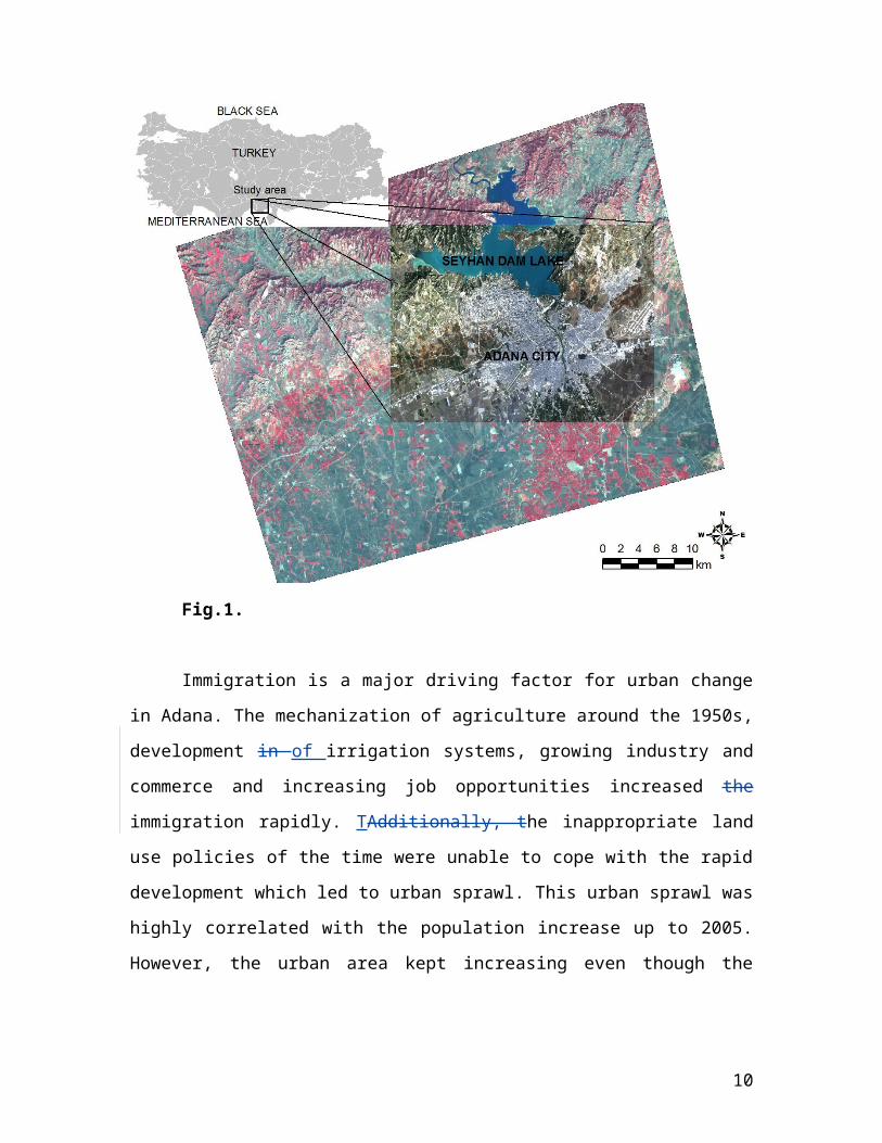
Geographically, Adana is located at the Southeastern Mediterranean coast of

Turkey. The region covers latitudes and longitudes are 36°00'- 37°30'N and and

longitudes 34°30'- 36°00'E respectively. The city is situated on the River Seyhan,

30 kilometers inland from the Mediterranean Sea. Adana Province has a population of

1.56 million, making it the fifth most populous city in Turkey (Fig. 1). Adana is nestled

in the most fertile area of the country, on land irrigated by the Seyhan. The southern part

of the province is entirely flat with various crops such as citrus, vegetables, maize, cotton

and wheat.

Fig.1.

6

Immigration is a major driving factor for urban change in Adana. The

mechanization of agriculture around the 1950s, development in of irrigation systems,

growing industry and commerce and increasing job opportunities increased the

immigration rapidly. TAdditionally, the inappropriate land use policies of the time were

unable to cope with the rapid development which led to urban sprawl. This urban sprawl

was highly correlated with the population increase up to 2005. However, the urban area

kept increasing even though the population increase gradually slowed down after 2005

(Fig. 2).

0

20

40

60

80

100

120

140

160

180

1965 1975 1985 1995 2007Time Periods

Area

0

200,000

400,000

600,000

800,000

1,000,000

1,200,000

1,400,000

1,600,000

Popu

latio

n

Area (km2) Population

Fig. 2.

3.2. Data Set and Spatial Variables

The data for this study comprised five different remotely sensed images recorded

on: 18 August 1967, 24 August 1977 (Corona satellite photos with 2-4m spatial

resolution), 25 November 1987 and 27 July 1998 (SPOT 1 with a 20 m spatial resolution

and panchromatic band of SPOT 4 with a 10 m spatial resolution) and 22 February 2007

(10 m spatial resolution ALOS AVNIR). In addition, we used 1:25,000 scale topographic

maps for deriving the Digital Elevation Model (DEM) calculation. Different resolutions

of data was were selected for the study area due to lack of high resolution historical

remotely sensed data (Table 1).

7

The input data variables and resolution were kept constant all throughout each of

the modeling approaches to ensure comparability among the five techniques.

Input data with high spatial resolution were was classified and spatial variables

were also prepared in their original resolutions and then resampled to a common scale

cell size of 10 m by using Nearest Neighbor (for classification) and Cubic Convolution

(spatial variables) methods. The models were calibrated and predicted in at the same

common spatial resolution of 10 m.

Table 1. Remotely sensed dataset.

Date of acquisition Data Source Spatial resolution18 August 1967,24 August 1977 Corona satellite photo 2-4m

25 November 1987,27 July 1998

SPOT 1 and SPOT 4 images (with 10 m panchromatic band)

20m

22 February 2007 ALOS AVNIR-2 10m

Establishment of the multivariate spatial model relies relied on integrating various

spatial variables to derive the overall probability of urban development for each pixel.

DEM, slope, excluded layer, urban extent, transportation, hillshade, distance to urban,

road and water maps were defined as spatial variables that influence the future urban

development of Adana City. Hillshade was included, even though it is only input to

SLEUTH model to increase the visual interpretation of the output. SLEUTH has

necessary pre-defined inputs that make the model run i.e. it requires a transportation layer

for distance calculation whereas, other methods useuses road distance. The other four

approaches have flexibility of in integrating various inputs. However our research utilized

the similar inputs as SLEUTHs to ensure comparison of among the techniques. Also

Tthese inputs are the main physical driving factors of urban growth which makes it

applicable for different cities all over the world like Sidney (Liu and Phinn, 2004),

Alexandria (Azaz, 2004), Iran (Rafiee et al., 2009), Cape Town (Watkiss, 2007), Houston

8

(Oğuz et al., 2007), Adana (Akın, 2011), and Hyderabad (Gandhi and Suresh, 2012).

Table 2 shows each spatial variable associated with a the different modeling approaches

in detail.

Model inputs are were derived from the same point in time. For all models, the

initial or “seed” year is was 1967 and the spatial variables (road distance, urban distance

etc.) were calculated twice considering the relevant prediction year. A 2007 prediction

was performed for accuracy assessment. Images recorded in 1977 and 1987 were only

used for the SLEUTH model as it requires at least four urban extent and two

transportation layers for different time periods. These explain the time differences in the

table 2.

Table 2. Model inputs for different model approaches.

Model USED Model Inputs SourceData Year

2007 (For accuracy) 2023

[SLEUTH]

SlopeLand useExcluded layerUrban extent Transportation Hillshade

Computed from DEM(Optional, not used here)Masked from classified mapMasked from classified mapDigitized from remotely sensed dataComputed from DEM

2007

19981967-19981967-1998

2007

2007

20071967-20071967-1998

2007

[Markov ChainLR,RT,ANN]

Slope Excluded layerUrban Distance Road DistanceWater DistanceDEM

Computed from DEMMasked from classified mapCalculated from urban extentCalculated from transportationCalculated from classified mapComputed from 1:25.,000 digitized topographic map

200719981998199819982007

200720072007200720072007

4. Method

This study can be summarized into four phases as: (i) geometric correction of the

multitemporal remotely sensed images, (ii) creation of urban maps derived from an object

based classification approach to determine the urban change detection with a ten year

9

interval, (iii) preparation of the spatial variables for modeling, (iv) model calibration,

validation and predicting urban development for the year 2023 with different modeling

approaches, (v) comparison of future modeling prediction results and selection of the

most appropriate model for the study area (Fig. 3).

Fig 3.

Urban The urban map, DEM etc. were determined as basic variables. Urban

distance, road distance, and water distance was were calculated by using basic variables

like urban extent and transportation layers.

10

A Markov Chain is a series of random values whose probabilities at a time

interval depend on the value of the number at the previous time (Fan 2008). The key

factor for a Markov chain is the transition probability matrix which defines change trends

from the past to today and into the future for a certain class type for each pixel. The

probability matrix is a set of conditional probabilities for the cells in the model to go

change to a particular new state. Markov modeling needs defined land use suitability

maps for each class. MCE was used to build these suitability maps. Distance from each

pixel to the urban, road and water classes, plus the DEM, slope and land use maps (as an

excluded layer) were defined as factors. These variables are common for each modelling

approaches. Water resources (the reservoir and distribution channels), green belts and

existing urban settlements were defined as limits. The weighting was determined

according to the historical land use change data based on the expansion pattern and the

observed land use transformations.

The SLEUTH model is implemented as a computer program written in the C

language, available as Open Source via the SLEUTH web site. The program operates as a

set of nested loops: the outer control loop repeatedly executes each growth “history”,

retaining cumulative statistical data, while the inner loop executes the growth rules for a

single “year.” The rules apply to onea cell at a time and the whole grid is updated as the

“annual” iterations complete. The modified array forms the basis for urban expansion in

each succeeding year. Potential cells for urbanization are selected at random and the

growth rules evaluate the properties of the cell and its neighbors (e.g., whether or not they

are already urban, what their topographic slope is, how close they are to a road). The

decision to urbanize is based on mechanistic growth rules as well as a set of weighted

probabilities that encourage or inhibit growth (Clarke and Gaydos 1998). Five factors

control the behavior of the system and four types of growth are defined in the model

(Table 3).

Table 3. Sequential growth types and controlling coefficients in the UGM (Jantz et al. 2003).

Growth cycle order Growth Type Controlling coefficient Description

1 Spontaneous Dispersion, slope resistanceRandomly selects cells for new growth

11

2 Diffusive Breed, slope resistanceExpansion from cells urbanized in spontaneous growth

3 Organic Spread, slope resistanceExpansion from existing settlements

4Road-influenced

Road gravity, dispersion, breed and slope resistance

Growth along transportation network

Logistic regression describes the relation between a categorical or qualitative

outcome variable and one or more predictor variables (Peng and So, 2002).

LR is a special case of multiple regression in which the dependent variable is discrete,

such as land cover types. If the dependent variable is dichotomous, y takes 1 and 0

values.

Logistic regression can be used only with two types of target variables:

1. A categorical target variable that has exactly two categories (i.e., a binary or

dichotomous variable).

2. A continuous target variable that has values in the range 0.0 to 1.0 representing

probability values or proportions.

In the case of n independent variables, the logistic regression equation can be expressed

as follows:

Logit (p) = ln(p/(1-p)) = a+b1*x1+ b2*x2+ bn*xn (2)

where p is the dependent variable expressing the probability that Y=1, x1, x2, and xn are the

independent variables; a is the intercept and b1, b2 and b3 are the coefficients of the

independent variables x1, x2, and xn respectively. The relationship between the dependent

variable and independent variables follows a logistic curve. The logit transformation of

the equation effectively linearizes the model so that the dependent variable of the

regression is continuous in the range of 0-1 (Eastman 2005).

Regression tree is a technique for modeling the probability of an event in terms

of predictor variables and uses repeated resampling of the data to develop empirical

sampling distributions of the relevant statistics in place of the distributional assumptions

(Joel et al. 1994). The regression tree algorithm conducts a binary recursive partitioning

and produces a set of rules and regression models to predict a target variable (historical

landuse change data) based on training data. Each rule set defines the conditions under

which a multivariate linear regression model is established for prediction (Yang et al.

12

2003; Breiman et al. 1984). “The goal in RT is to use a set of predictor variables to

estimate the means of one or more response variables. A binary tree is constructed by

repeatedly splitting the data set into subsets. Each individual split is based on a single

predictor variable and is chosen to minimize the variability in the response variables in

each of the resulting subsets. The tree begins with the full data set and ends with a series

of terminal nodes. Within each terminal node the means of the response variables are

taken as the predictions for observations” (Michaelsen et al., 1994).

ANNs were first discussed by Rosenblatt (1958), who introduced the concept of

the perceptron. His single perceptron was able to classify only linearly separable data,

which was an important limitation to its use. Nonlinear data separation was achieved in

the 1980s as a result of increased computing power and the development of new

algorithms and network topologies. This enabled the use of ANNs for the classification of

remotely sensed imagery (Key et al. 1989; Benediktsson et al. 1990). The multi-layer

perceptron described by Rumelhart et al. (1986) is the most commonly encountered ANN

model in remote sensing. This type of ANN model consists of an input layer, one or more

hidden layers and an output layer. Each layer consists of processing elements called units

or nodes. It holds input values and distributes the information to all units in the next

layer. The input values can be spectral bands or additional information such as image

texture measures. The output layer comprises the land cover classes or in the study case,

transition probability matrix for a specific land use transformation. Layers between input

and output layers are termed as hidden layers. The number of hidden layers within the

network are is defined by the user.

4.1. Object based classification and urban growth change

The object-based classification approach involves the integration of vector and

raster data within a GIS environment and this approach enabled enables the extraction of

image object primitives at different spatial resolutions, termed multi-resolution

segmentation. (Bian and Walsh 1992).

The next stage involved involves a supervised object based classification with the

nearest neighbor algorithm. In our classification, eEach image object was assigned to

13

settlement, agriculture, citrus, forest, bare ground, green belt, water and road classes (Fig.

4).

Fig.4.

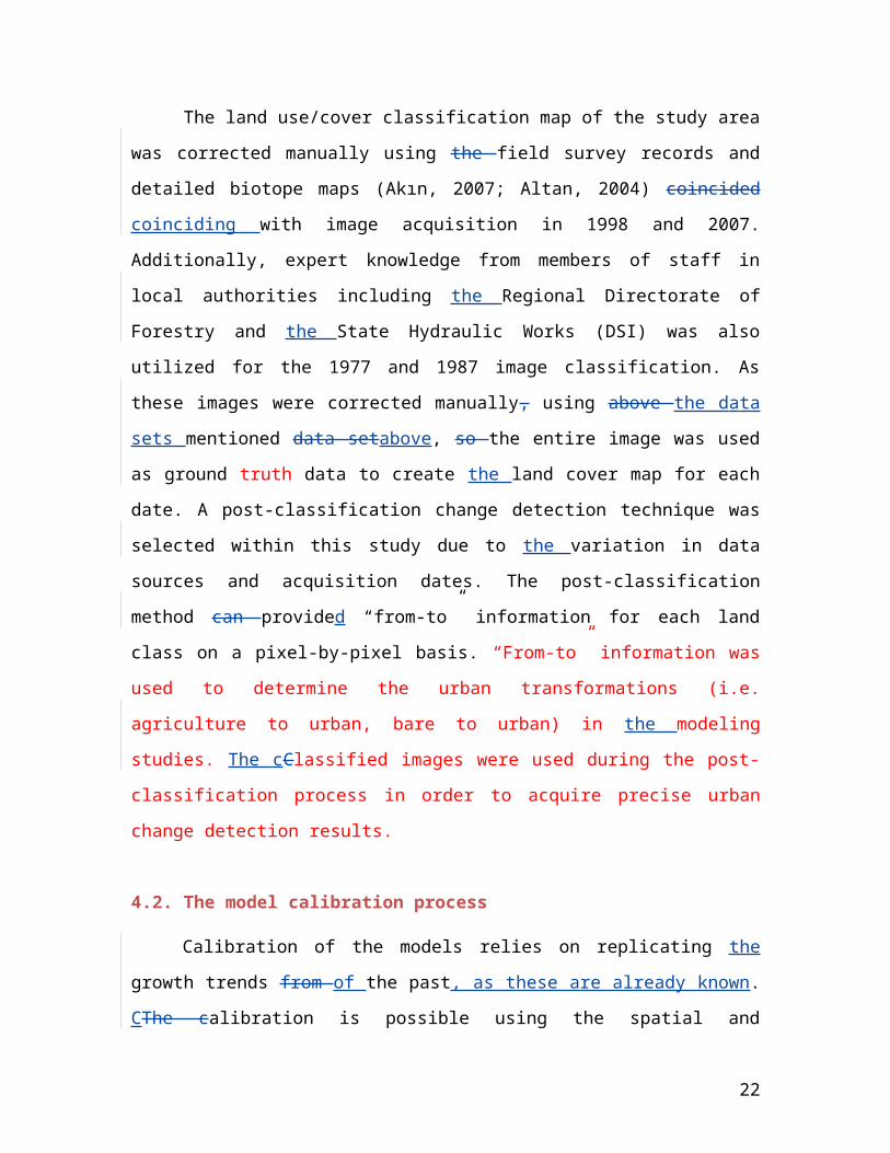
The land use/cover classification map of the study area was corrected manually

using the field survey records and detailed biotope maps (Akın, 2007; Altan, 2004)

coincided coinciding with image acquisition in 1998 and 2007. Additionally, expert

knowledge from members of staff in local authorities including the Regional Directorate

of Forestry and the State Hydraulic Works (DSI) was also utilized for the 1977 and 1987

image classification. As these images were corrected manually, using above the data sets

mentioned data setabove, so the entire image was used as ground truth data to create the

14

land cover map for each date. A post-classification change detection technique was

selected within this study due to the variation in data sources and acquisition dates. The

post-classification method can provided “from-to” information for each land class on a

pixel-by-pixel basis. “From-to” information was used to determine the urban

transformations (i.e. agriculture to urban, bare to urban) in the modeling studies. The

cClassified images were used during the post-classification process in order to acquire

precise urban change detection results.

4.2. The model calibration process

Calibration of the models relies on replicating the growth trends from of the past,

as these are already known. CThe calibration is possible using the spatial and statistical

properties of the past to ‘predict’ the known present. Once the most descriptive weighting

values are set to understand urban change over time, these values are used to forecast

future growth. The calibration processes of the Markov Chain, LR, RT and ANN,

resulted in a transition probability maps (TPM) values that best simulate “historical

growth” for the region.

4.2.1. Markov Chain Model

For the Markov Chain TPM calculation, first a cross tabulation is undertaken

between the land cover maps for two dates. “From this, the basic transition probability

matrix (x) is calculated using the table entries and the marginal totals. If the projected

time period is in between even multiples of the training period, then the power rule is

used to generate 3 transition matrices that envelop the projection time period. If the 3

time periods are times A (1967), B (2007) and C (2023), the period to be interpolated will

be between A and B. The three values at each cell in the transition probability matrix are

then fed into a quadratic regression (thus there will be a separate regression for each cell).

Given that a quadratic regression (Y=a+b1X+b2X2) has 3 unknowns and we have three

data points, it yields a perfect fit. This equation is then used to interpolate the unknown

transition probability” (Takada et al., 2010).

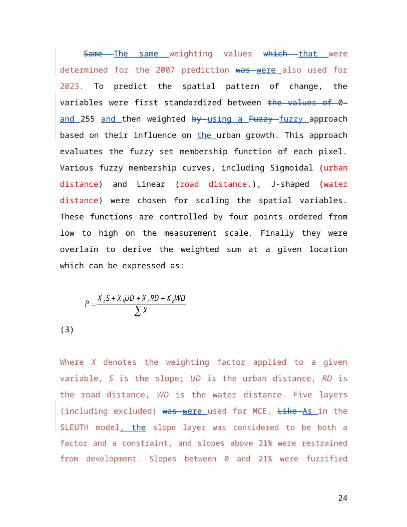
Same The same weighting values which that were determined for the 2007

prediction was were also used for 2023. To predict the spatial pattern of change, the

15

variables were first standardized between the values of 0- and 255 and then weighted by

using a Fuzzy fuzzy approach based on their influence on the urban growth. This

approach evaluates the fuzzy set membership function of each pixel. Various fuzzy

membership curves, including Sigmoidal (urban distance) and Linear (road distance.), J-

shaped (water distance) were chosen for scaling the spatial variables. These functions are

controlled by four points ordered from low to high on the measurement scale. Finally

they were overlain to derive the weighted sum at a given location which can be expressed

as:

(3)

Where X denotes the weighting factor applied to a given variable, S is the slope; UD is

the urban distance, RD is the road distance, WD is the water distance. Five layers

(including excluded) was were used for MCE. Like As in the SLEUTH model, the slope

layer was considered to be both a factor and a constraint, and slopes above 21% were

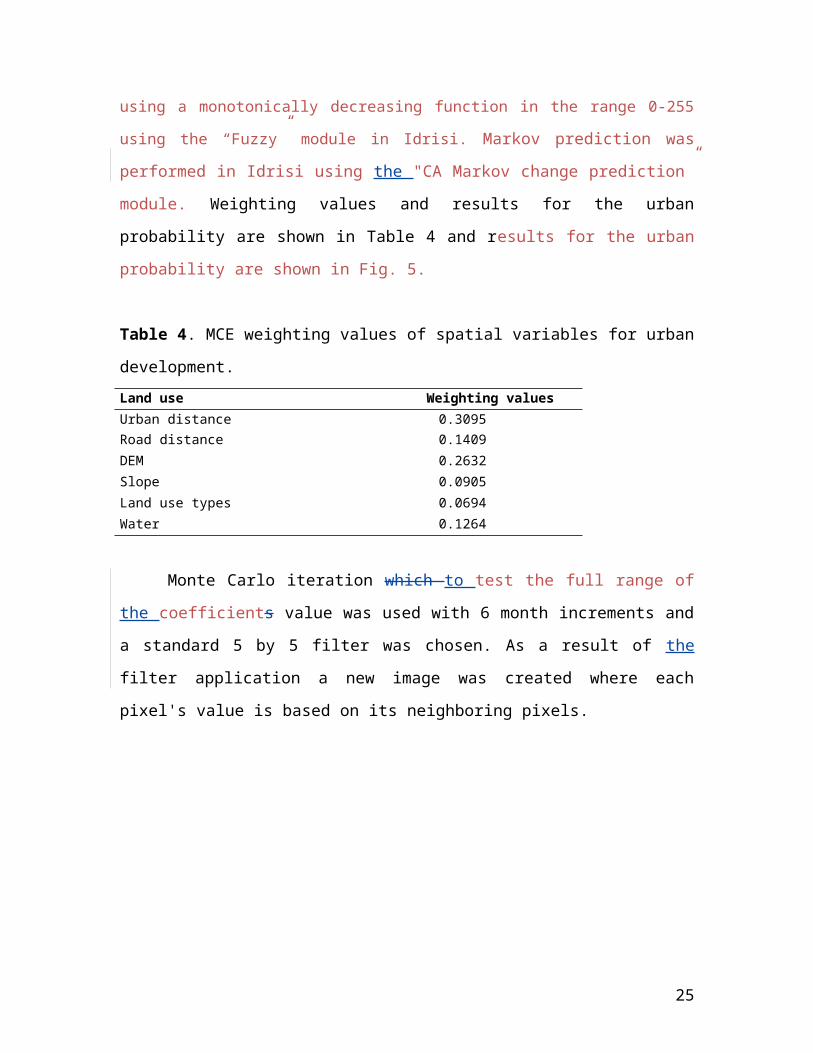
restrained from development. Slopes between 0 and 21% were fuzzified using a

monotonically decreasing function in the range 0-255 using the “Fuzzy” module in Idrisi.

Markov prediction was performed in Idrisi using the "CA Markov change prediction”

module. Weighting values and results for the urban probability are shown in Table 4 and

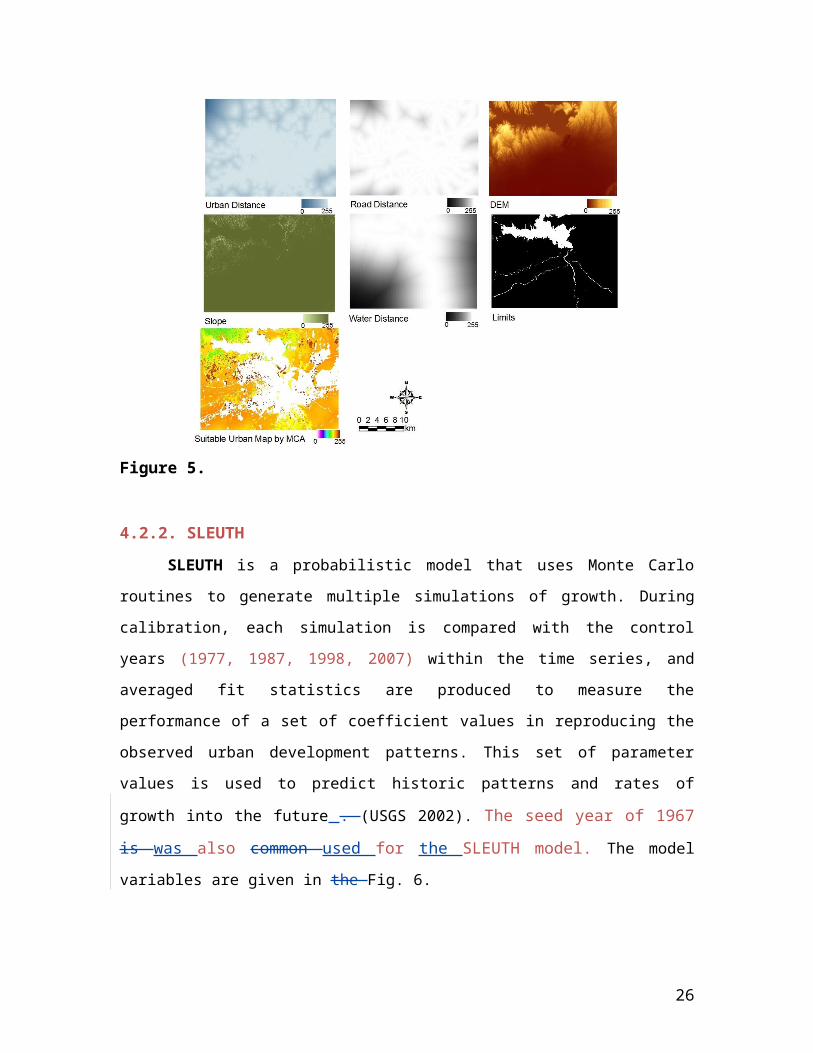
results for the urban probability are shown in Fig. 5.

Table 4. MCE weighting values of spatial variables for urban development.

Land use Weighting valuesUrban distance 0.3095Road distance 0.1409DEM 0.2632Slope 0.0905Land use types 0.0694Water 0.1264

Monte Carlo iteration which to test the full range of the coefficients value was used with 6 month increments and a standard 5 by 5 filter was chosen. As a

16

result of the filter application a new image was created where each pixel's value is based

on its neighboring pixels.

Figure 5.

4.2.2. SLEUTH

SLEUTH is a probabilistic model that uses Monte Carlo routines to generate multiple

simulations of growth. During calibration, each simulation is compared with the control years

(1977, 1987, 1998, 2007) within the time series, and averaged fit statistics are produced to

measure the performance of a set of coefficient values in reproducing the observed urban

development patterns. This set of parameter values is used to predict historic patterns and

rates of growth into the future . (USGS 2002). The seed year of 1967 is was also common

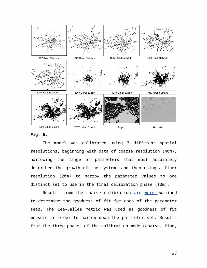
used for the SLEUTH model. The model variables are given in the Fig. 6.

17

Fig. 6.

The model was calibrated using 3 different spatial resolutions, beginning with

data of coarse resolution (40m), narrowing the range of parameters that most accurately

described the growth of the system, and then using a finer resolution (20m) to narrow the

parameter values to one distinct set to use in the final calibration phase (10m).

Results from the coarse calibration are were examined to determine the goodness

of fit for each of the parameter sets. The Lee-Sallee metric was used as goodness of fit

measure in order to narrow down the parameter set. Results from the three phases of the

calibration mode (coarse, fine, final and derive) are presented in table 5 which presents

the highest scores from model runs.

18

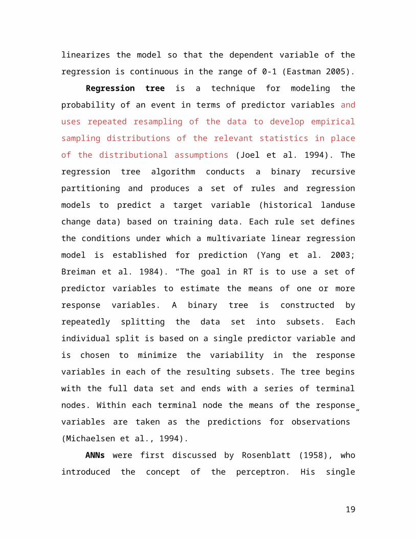
Table 5. Final calibration results and coefficient values for final and drive phases.

Product Compare Pop Edges Cluster Cluster Size LeesaleeCoarse 0.006 0.97678 0.99147 0.07394 0.60499 0.90081 0.41352Fine 0.02135 0.89927 0.9931 0.69567 0.75976 0.77954 0.40686Final 0.03838 0.89453 0.99362 0.64 0.7428 0.75544 0.40249

Slope %Urban Xmean Ymean Rad FmatchCoarse 0.93925 0.99134 0.7234 0.94417 0.9905 0.58997Fine 0.81331 0.99269 0.73476 0.40451 0.99203 0.5991Final 0.87589 0.99326 0.70301 0.8262 0.99245 0.59566

Diff Brd Sprd Slp RGCoarse 1 25 50 100 50Fine 1 25 60 50 25Final 1 24 62 38 30Derive 1 30 62 48 25

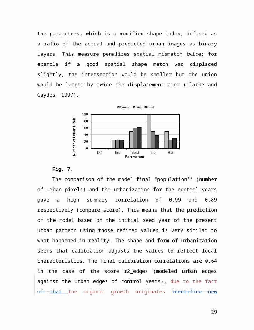
Tables Table 5 shows successive improvement in the parameters that control the

behavior of the system, although some measures decline at higher resolutions. (Fig. 7).

The Lee Sallee (Lee and Sallee, 1970) value was used to narrow the parameters, which is

a modified shape index, defined as a ratio of the actual and predicted urban images as

binary layers. This measure penalizes spatial mismatch twice; for example if a good

spatial shape match was displaced slightly, the intersection would be smaller but the

union would be larger by twice the displacement area (Clarke and Gaydos, 1997).

Fig. 7.

The comparison of the model final “population’’ (number of urban pixels) and the

urbanization for the control years gave a high summary correlation of 0.99 and 0.89

respectively (compare_score). This means that the prediction of the model based on the

initial seed year of the present urban pattern using those refined values is very similar to

what happened in reality. The shape and form of urbanization seems that calibration

19

adjusts the values to reflect local characteristics. The final calibration correlations are

0.64 in the case of the score r2_edges (modeled urban edges against the urban edges of

control years), due to the fact of that the organic growth originates identified new

structures and it is difficult to replicate these compared to known urban, and 0.74 in the

case of the cluster_r2 score (modeled number of urban clusters against known number of

urban clusters). The A high value of 0.99 for %Urban was acquired which is the least

squares regression of percentage of available pixels urbanized compared to the urbanized

pixels for the control years. For the Lee-Sallee value (degree of shape match between the

modeled growth and the known urban extent) 0.40 was achieved. Other studies have

shown that (Clarke and Gaydos, 1998, Silva and Clarke, 2002) it is difficult to obtain

high values of shape match (Clarke and Gaydos, 1998, Silva and Clarke, 2002). The A

value of 0.40 for the Lee-Sallee metric was equal to or better than that achieved in other

comparable SLEUTH applications.

The urbanization of the metropolitan area tended to occur outward from the main

nucleus and along the main transportation infrastructure. This explains why the final

spread_coefficient is was as high as 62.

4.2.3. LR, RT and ANN Models

CA modelling is the simulation process of the The LR, RT and ANN models.

They use similar steps in order to carry out the urban simulation with different level of

merits. The models were trained using predetermined spatial variables as inputs to

produce five probability maps as an outputs. First, a comparison of LULC maps derived

from two different dates (1967 and 1998; 1967 and 2007) were was performed and then

change analysis used to is conducted to identify the most effective urban growth

transformations like , such as i. agriculture to urban; ii. citrus to urban; iii. forest to urban;

iv. bare to urban; v. green to urban. Land use transformations is usually dependent on a

series of spatial variables in terms of proximityies. Each spatial variable took a weighting

value according to these transformations and the TPM was calculated for each of them.

Also for the training process, small descriptive subsets were extracted (Fig.8). The

models require continuous quantitative variables. For the prediction, the TMP maps were

overlaid together and served as a single map during the application. For LR, Idrisi

20

software; for RT, See5 and the Erdas Imagine NLSD tool and for ANN, MATLAB

software was used.

Figure 8. 2023 calibration process for the LR, RT and ANN models.

The TPMs was then integrated into a CA simulator Dinamica EGO 1.4.0 for the

future urban growth predictions. Expander and Patcher tools were used for the CA

simulation (Fig.9).

Fig.9.

Dinamica EGO (Environment for Geoprocessing Objects) which is written in C++

and Java, holds a series of algorithms called functors and composed of two

complementary “functors” the Expander and the Patcher, which are set to the average

size of patches, stains and the variances of the isometry. Increasing the patch size and

21

variance creates a less fragmented and a more diverse landscape. Isometry greater than

one gives more isometric patches. The first process is dedicated only to the expansion or

contraction of previous patches of a certain class, while the second process is designed to

generate or form new patches through a seeding mechanism. The Patcher searches for

cells around a chosen location for a joint transition. The process is started by selecting the

core cell of the new patch and then selecting a specific number of cells around the core

cell, according to the TPM (Dinamica, 2013).

The combination of the two processes is shown in the equation below (Filho et al.,

2013) :

Qij=r*(Expander Function)+s*(Patcher Function) (4)

Where Qij Stands for the number of transitions of type ij specified per simulation

step and r and s represent respectively the percentage of transitions executed by each

function, being that r+s=1. Both functions incorporate an allocation device which is

responsible for locating the cells with the highest transition probabilities for the given

transition. One step of Dinamica prediction corresponds to one year.

Dinamica EGO has successfully been applied in numerous environmental studies.

Examples of Dinamica EGO application include modeling tropical deforestation in the

Amazon from local to basin-wide scales (Soares-Filho et al., 2010 ); land use and cover

change in the Atlantic Forest (Texeira et al., 2009) and in the tropical dry forest of

Mexico (Cuevas et al., 2008); urban dynamics (Almeida et al., 2005; Godoy and Soares-

Filho, 2008); logging in the Amazon (Merry et al., 2009), and forest fire risk (Silvestrini

et al., 2011).

The calibration process was repeated for accuracy assessment. In other words, the

1967-1998 calibration was performed for the 2007 prediction (validation) and the 1967-

2007 calibration was performed for the 2023 prediction. Urban change and related spatial

variables were defined as response and predictor variables respectively. Multiple

regression tree models were built using various pruning and input band combinations.

500 randomly sampled pure pixels per class were used as training data, and 250 pixels

per class formed the testing data.

A rule set of conditions under each regression tree model was built. Error

estimates of the regression tree predicted probability images were made for model

22

validation. The average absolute error of the 2007 and 2023 probability image prediction

(by comparing model prediction against “true” values from the test data) are given in

table 6 (Cl refers to Class).

Table 6. Error and correlation matrix for Regression Tree.

1967-1998 1968-2007Cl1 Cl 2 Cl 3 Cl 4 Cl 1 Cl 2 Cl 3 Cl 4

Average error 19.4 6.7 5.8 2.4 22.6 6.5 4.8 0.7Relative error 0.3 0.32 0.36 0.49 0.29 0.32 0.3 0.28Correlation coefficient 0.89 0.85 0.8 0.63 0.9 0.85 0.86 0.87

Two rules generated from the regression tree model are presented here as an example:

Rule 1: [26319 cases, mean 0.1, range 0 to 10, est err 0.1] if

band02 <= 253 then

dep = 0.1

Rule 100: [741 cases, mean 212.4, range 83 to 250, est err 26.2] if

band03 > 220band04 > 179band06 > 27band06 <= 29band07 > 219

thendep = 1007.3 - 19.56 band06 - 1.23 band03 + 0.2 band07

where dep is defined as the response variable and presents historic urban change in the

model. The average absolute error of the urban change probability map prediction was

measured as 13% by comparing the model prediction of the known year against real

values from the test data.

With the LR, ROC (Receiver operating characteristic) statistics were obtained

after creating the probability maps for the time period of 1967-2007 (Table 7).

Table 7. Regression statistics for different time periods.Regression Statistics 1967-2007

Observed Fitted 0 Fitted 1 Percent correct0 175768 36471 82.811 31195 70147 69.21

23

ROC 0.82

The ROC method has been introduced to LULC modeling to compute the correlation

between simulated and actual changes (e.g., Pontius and Schneider, 2001). ROC = 1

indicates a perfect fit and ROC = 0.5 indicates a random fit. A highest value of 0.82 was

obtained, which verifies the accuracy of the LR model. However, the comparison of

actual and future simulation maps did not yield the same accuracy as described in the last

section.

Through a training/learning process, the ANN adjusts the weight and bias values

at the nodes and so determines the best suitable transition rules and parameters. The

outputs of the network are compared and evaluated with the targets that are samples of

the real world, e.g. the urban change data in this study. Then, based on this comparison,

the weight and bias values of the network are adjusted in order to reduce the difference

between the network outputs and the targets. This process is repeated until the difference

between the outputs and the targets reaches a previously set goal (Guan et al., 2005).

MATLAB software was used for ANN training process. Variables were scaled to the

range of 0-1. The number of training cycles was set at 2000 (fig. 10).

Fig. 10.

5. Discussion

This study has significance for the study area because: (i) it represents the first

urban growth modeling study for Adana City that uses different modeling approaches; (ii)

historic urban changes were measured and prediction was made with high spatial

24

resolution remotely sensed data; (iii) there is a lack of studies that evaluate land use

changes and urban development over a longer term history, such as from 1960.

The change detection results showed that there is a growing trend toward urban

areas at the expense of agricultural land. Approximately 161 km2 of new urban area was

gained mainly from the productive agricultural areas around the city center. By itself, 112

km2 of agriculture areas were converted primarily to urban and a total of 145 km 2 were

lost during the time period of the study. A second large urban transformation took place

on the bare ground and in green belts adding 27 km2 and 15 km2 of new urban area

respectively. The spatial prediction results for urban expansion showed that urban areas

have been expanding continuously. The direction of expansion is around the existing

urban areas and along transportation routes. Organic growth is highly characteristic of

Adana city.

Once each model had successfully replicated past urban expansion, it was used to

project future development of urban land uses. The predictive accuracy of the model was

evaluated by comparing the predicted and the actual map of urban areas on a pixel basis

for 2007. Current urban extent was the key factor for the comparison. The ‘traditional’

error matrix and Kappa coefficient and multiple map comparisons were used to assess the

accuracy (Congalton 1991; Pontius et al. 2001). Allocation and Quantity Disagreement

maps were prepared as described by Pontius et al. (2008). Each modeling application was

assessed statistically using: 1) a reference map of the initial time (1967), 2) a reference

map of the subsequent time (2007) and 3) prediction map of subsequent time (2007).

Two-map comparisons for each application were performed to derive: 1) dynamics of the

model (observed change), 2) the behavior of the model (predicted change) and 3) the

accuracy of the prediction (Pontius et al, 2008; Pontius and Spencer 2005; Pontius and

Millones, 2011). The sum of two components of quantity disagreement and allocation

disagreement provided more clear interpretation of the model results relative to the

Kappa ratio as both components were present in parts of the study area (Pontius and

Millones, 2011).

Modeling results were compared for the year 2007 (Fig. 11). All models

overestimated the urban prediction results.

25

0 0.05 0.1 0.15 0.2 0.25 0.3 0.35

Observed

Markov(Predict)

Markov(Error)

SLEUTH(Predict)

SLEUTH(Error)

ANN(Predict)

ANN(Error)

LogisticR(Predict)

LogicticR(Error)

RegressionT(Predict)

RegressionT(Error)

Disaggrement (Proportions of Urban Class)

Quantity Allocation

Fig. 11.

When the models predict the observed change accurately, then predicted change is

identical to observed change. For LR and RT models, most of the observed change was

allocation disagreement. However, when considering the gain and loss of built values, the

SLEUTH and Markov models were the most consistent models with the real data. ANN

has the highest disagreement value compared with other models. For example, ANN, LR

and RT models have the observed change value of 138 km2, 141 km2 and 138 km2

respectively, while the actual observed change was calculated as 136 km2. These models

have the closest urban change value of the real change which is inadequate to compare

model performance. Thus, disagreements maps enable us to produce the distribution of

predicted change in addition to the quantity of change. Quantity and Allocation

Disagreements maps are shown in Fig. 12.

26

27

Fig. 12.

Kappa accuracies were also calculated. The most accurate results were achieved

by SLEUTH, Markov Chain and RT with Kappa accuracies of 0.7463, 0.7214, and

28

0.7108 respectively. LR and ANN did not meet the expectations with lower Kappa

accuracies of 0.6640 and 0.6586 for the urban class respectively (Table 8).

Table 8. Kappa Index of Agreement values for different modeling approaches.

Markov Chain ANN SLEUTH Logistic Regression

Regression Tree

2007 Predicted Urban class

(km2)156 138 146 141 138

Urban class accuracy (KIA) 0.72 0.66 0.75 0.66 0.71

One of the most important findings was that the SLEUTH accuracy is actually higher

than 0.7463. After the last step of the modeling, the SLEUTH prediction maps were

passed back into the GIS without any coordinate information. A second rectification

process was performed to the SLEUTH thematic simulation map for Kappa calculation in

order to ensure perfect overlay of the predicted and actual 2007 maps. Root-mean square

(RMS) error was found to be 1.3 pixels.

6. Conclusions

The objective of this research was to quantify the amount of urbanization (as

urban/non-urban) and to select an appropriate model for the fast growing Mediterranean

city of Adana. Five different modeling approaches were applied including Markov Chain,

SLEUTH, LR, RT and ANN within CA modeling and the results were compared and

evaluated to find most appropriate model for this region.

The models used for this study can be sorted into two general categories:

statistical (LR, RT, ANN) and stochastic models (Markov Chain, SLEUTH). In statistical

based models urban dynamics take place through a set of statistic variables and historic

change itself is the dependent variable. These models are more data oriented and also

present different degrees of fit for the change potential to observed past changes (Mas et

al., 2014). Stochastic models predict future urban land use based on probabilistic

estimates and rules.

Results from the future modelling suggest that the SLEUTH, Markov Chain and

RT models generate better prediction for urban growth compared with RT and ANN

29

models. From the calibration point of view, the Markov Chain is considered somewhat

subjective due to the preparation of suitability maps using the weighting values which

need to be defined by the user. Once the proper weighting values are managed based on

expert knowledge, detailed information about LULC change is acquired and the model

performance can be improved. Besides, there is a growing approval that knowledge-

driven approaches like Markov Chains are more controllable than machine learning

approaches like ANN. (Vega at al., 2012; Mas et al., 2014; Arsanjani et al., 2013, Akın,

2012). Also, the rates of the observed change during the calibration are assumed to be

stable with the Markov method. The Markov chain approach led to an urban area of 59

km2 for 2023 (2023-2007) and 156 km2 (2007-1967) for 2007. The observed urban

change between 1967-2007 time period was 136 km2.

The most outstanding advantage of the SLEUTH model is the ability to get

periodic historical urban extent data as the control data during the calibration. Roughly

ten years increments separated the data layers used, i.e., including 1967, 1977, 1987,

1998 and 2007. The model is calibrated year by year. There are thirteen elements that

measure best fit statistics by comparing historical data and simulated growth. So, no

additional validation process is required. But in order to ensure comparability, KIA and

Allocation and Disagreement maps were applied. Boom and bust values were determined

only with the SLEUTH model. For the study, only historic change trends were

considered. Scenario development in the model is embedded within the excluded layers.

If the user does not use a scenario layer, then the model assumes the same growth trend

as in the past. One of the disadvantages for the SLEUTH model is that the calibration

process was time consuming. Recent SLEUTH model developments promise to reduce

this time considerably. The SLEUTH model application resulted in 146 km2 of total

urban area for 2007 and 75 km2 for 2023 respectively.

The advantage of the RT, RT and ANN techniques is the capacity to explore the

relationships between LULC transformations and their causative factors quantitatively,

which enables us to distinguish between the spatial variables (Park et al., 2011, Arsanjani

et al., 2013). Integrating the desired number of variables is possible. Weighting of the

spatial variables was performed objectively without any user knowledge. Determination

of the historic change map for the training is the key factor of the TPM calculation. Also

30

an additional CA predictor module or software is required for the future growth

estimation. These groups of models suffer from several limitations such as temporal

determination, quantification and allocation of change (Arsanjani et al., 2013; Hu and Lo,

2007). Exporting the outputs into a CA model eliminated this deficiency. Like the

Markov model, using a single period of data for the TPM can lead to forecasts that are

short-term and to discontinuous trends. Predictions based on a period of strong growth or

decline may tend to overshoot or undershoot the actual LULC change trends (Iacono et

al., 2012). Defining boom and bust values with multiple period data would prevent the

over/under estimation of the prediction maps substantially. Also, more descriptive

variables for the target state may increase the accuracy of the RT, RT and ANN models.

RT simulated urban growth for 2023 and 2007 with an area of 51 km2 and 138 km2; LR

simulated an area of 226 km2 and 164 km2; ANN simulated an area of 40 km2 and 138

km2 respectively.

According to the 1:100,000 regional plans, the development of the Northwestern

side of the study area is very likely. These pixels are mostly threatened agricultural areas

and have the highest urban probability values due to their closeness to the existing urban

pixels. Among the five techniques, SLEUTH was the most accurate one in predicting

these pixels as urban.

Different modeling approaches have their own merits and no single approach is

appropriate for all cases. In practice, different modeling approaches are often compared

to find the most useful results for a specific location. The selection of an appropriate

modeling technique is important. This study provided a better understanding of the

various techniques within a densely populated Mediterranean city. We hope that these

conclusions, forecasts and results are of use in other sustainable environmental planning

studies. In future work, we hope to better integrate physical and socio-economic variables

into the modelling approaches.

REFERENCES

31

Almeida, C. M., Gleriani, J. M., 2005. Cellular automata and neural networks as a

modelling framework for this simulation of urban land use change. Anais XII

Simpósio Brasileiro de Sensoriamento Remoto, Goiânia, Brasil, INPE, 3697-

3705.

Almeida, C. M., Gleriani, J. M., Castejon, E. F., and Soares-Filho, B. S. (2008). Using

neural networks and cellular automata for modelling intra-urban land-use

dynamics. International Journal of Geographical Information Science, 22(9), 943-

963.

Balzter, H., Braun, P. W., Kohler, W., 1998. Cellular automata models for vegetation

dynamics. Ecological Modeling 107, 113–125.

Batty, M., Couclelis, H., Eichen, M., 1997. Urban systems as cellular automata.

Environment and Planning B 24, 159–164.

Batty, M., Xie, Y., 1994. From cells to cities. Environment and Planning B: Planning and

Design 21, 531–548.

Bian, L., Walsh, S. J., 1992. Scale dependencies of vegetation and topography in

mountainous environment of Montana. Professional Geographer 45, 1–11.

Bourne, L. S., 1976. Monitoring change and evaluating the impact of planning policy on

urban structure: a markov chain experiment. Plan Canada 5–14.

Breiman, L., Friedman, J. H., Olshen, R. A., Stone, C. J., 1984. Classification and

Regression Trees. Wadsworth, Belmont.

Clarke, K. C., Hoppen, S., Gaydos, L., 1997. A Self-modifying cellular automaton model

of historical urbanization in the San Francisco Bay Area. Environmental and

Planning B 24, 247–261.

Clarke, K. C, Gaydos, L. J., 1998. Loose-Coupling a cellular automaton model and GIS:

long-term urban growth prediction for San Francisco and Washington/ Baltimore”

International Journal of Geographical Information Science 12, 699–714.

Congalton, R. G., 1991. A review of assessing the accuracy of classifications of remotely

sensed data. Remote Sensing Environment 37, 35–46.

Couclelis, H., 1997. From cellular automata to urban models: new principles for model

development and implementation. Environment and Planning B: Planning and

Design, 24 165-174.

32

Cuevas S G, Mas J-F., 2008. Land use scenarios: a communication tool with local

Communities. In: Paegelow M. & Camacho Olmedo M.T., Ed. Modelling

Environmental Dynamics, Springer-Verlag,.

Chen, Y., Li, X., Liu, X., Ai, B., 2013. Modeling urban land-use dynamics in a fast

developing city using the modified logistic cellular automaton with a patch-based

simulation strategy. International Journal of Geographical Information Science.

Dinamica Project, 2013. http://www.csr.ufmg.br/dinamica/

Eastman, J. R., McKendry. J., Fulk, M. A., 2005. Change and time series analysis.

Explorations in Geographic Informations Systems Technology. Geneva, United

Nations Institude for Training and Research (UNITAR).

Fan, F., Wang, Y., Wang, Z., 2008. Temporal and spatial change detecting (1998–2003)

and predicting of land use and land cover in Core corridor of Pearl River Delta

(China) by using TM and ETM+ images. Environmental Monitoring and

Assessment 137, 127–147.

Gilpin, M. E., 1990. Extinction of finite meta populations in correlated environments in

Shorrocks, B., Swingland, I.R. (Eds.), Living in A Patchy Environment. Oxford

University Press, New York, 177–86.

Guan, Q., Wang, L. and Clarke, K. C. (2005) An Artificial-Neural-Network-based,

Constrained CA Model for Simulating Urban Growth . Cartography and

Geographic Information Science, 32, 4, 369-380.

Hemphill, J. J., Clarke, K. C., Gazulis, N., Oguz, H., Dietzel, C., 2005. Diffusion and

coalescence of the Houston Metropolitan Area: evidence supporting a new urban

theory. Environment and Planning B: Planning and Design 32, 231-246.

Itami, R. M., 1994. Simulating spatial dynamics: cellular automata theory. Landscape

and Urban Planning 30, 24– 47.

Jantz, C, J., Goetz, S. J., Smith, A, J., Shelly, M., 2003. Using the SLEUTH Urban

growth model to simulate the impacts of future policy scenarios on land use in the

Baltimore-Washington metropolitan area. Environment and Planning B 31, 251-

271.

33

Li, X., Yeh, A. G., 2000. Modeling sustainable urban development by the integration of

constrained cellular automata and GIS. International Journal of Geographical

Information Science 14, 131-152.

Li, X., Yeh, A. G., 2002. Neural-network-based cellular automata for simulating multiple

land use changes using GIS, International Journal of Geographical Information

Science 16, 323-343.

Li, X., Liu, X., 2006. An extended cellular automaton using case-based reasoning for

simulating urban development in a large complex region. International Journal of

Geographical Information Science 20, 1109 -1136.

Liu H, Zhou Q, 2005, “Developing urban growth predictions from spatial indicators

based on multi-temporal images” Computers, Environment and Urban Systems 29

580–594.

Merry, F.; Soares-Filho, B. S.; Nepstad, D.; Aamacher, G.; Rodrigues, H. Balancing

Conservation and Economic Sustainability: The Future of the Amazon Timber

Industry. Environmental Management, EUA, 44 (3): 395-407.2009.

Michaelsen, J., Schimel, D. S., Friedl, M. A., Davis, F. W. and Dubayah, R. C. (1994),

Regression Tree Analysis of satellite and terrain data to guide vegetation sampling

and surveys. Journal of Vegetation Science, 5: 673–686.

Muller, R. M., Middleton, J., 1994. A Markov model of land-use change dynamics in the

Niagara region. Ontario, Canada. Landscape Ecology 9, 151–157.

Olden, J. D., Jackson, D. A., 2001. Fish–habitat relationships in lakes: gaining predictive

and explanatory insight by using artificial neural networks. Transactions of the

American Fisheries Society 130, 878-897.

Peng, C.J., So, T,H., Logistic Regression Analysis and Reporting: A Primer.

Understanding Statistics, 1:31-70.

Pontius, R. G., Cornell, J. D., Hall, C. A. S., 2001. Modeling the spatial pattern of land-

use change with geomod2: application and validation for Costa Rica agriculture.

Ecosystems and Environment, 1775 1–13.

Pontius, R. G., Shusas, E., McEachern, M., 2004. Detecting important categorical land

changes while accounting for persistence. Agriculture, Ecosystems and

Environment 101, 251–268

34

Pontius, R. G., Gilmore, R., Spencer, J., 2005. Uncertainty in extrapolations of predictive

land change models. Environment and Planning B: Planning and Design 32, 211-

230.

Pontius, R. G., Millones, M., 2011. Death to Kappa: birth of quantity disagreement and

allocation disagreement for accuracy assessment. Journal of Remote Sensing, 32:

4407-4429.

Pontius, R. G., Boersma, W., Castella, J. C., Clarke, C. K., Nijs, T., Dietzel, C., Duan, Z.,

Fotsing, E., Goldstein, N., Kok, K., Koomen, K., Lippitt, C. D., McConnell, W.,

Sood, A. M., Pijanowski, B., Pithadia, S., Sweeney, S., Trung, T. N., Veldkamp,

A. T., Verburg, P. H., 2008. Comparing the input, output, and validation maps

for several models of land change. The Annals of Regional Science 42, 11-47.

Rumelhart, D. E., Hinton, G. E, Williams, R. J., 1986. Learning representations by back-

propagation errors. Nature 323, 533-536

Ruxton, G. D., 1996. Effects of the spatial and temporal ordering of events on the

behaviour of a simple cellular automaton. Ecological Modeling 84, 311–314.

Shmueli, D., 1998. Applications of neural networks in transportation planning. Progress

in Planning 50, 141-204.

Silva, E. A., Clarke, K. C., 2002. Calibration of the SLEUTH urban growth model for

Lisbon and Porto, Portugal” Computers, Environment and Urban Systems 26,

525–552.

Silva, E. A., Clarke, C. K., 2005. Complexity, Emergence and Cellular Urban Models:

Lessons Learned from Appling SLEUTH to two Portuguese Cities. European

Planning Studies 13, 93-115.

Silvestrini, R.A.; Soares-Filho, B.S.; Nepstad, D.; Coe, M.; Rodrigues, H.O.; Assunção,

R. 2011. Simulating fire regimes in the Amazon in response to climate change and

deforestation. Ecological Applications, 21(5), 2011, pp. 1573–1590.

Soares-Filhoa, B., Moutinhob, P., Nepstadb, D., Andersond, A., Rodriguesa, H., Garciaa,

R., Dietzschb, L., Merrye, F., Bowmanc, M., Hissaa, L., Silvestrinia, R., and

Marettid, R. 2010. Role of Brazilian amozon protected areas in climate change

mitigation. Proceedings of the National Academy of the United states of America.

35

Stevens, D., Dragicevic, S., Rothley, K., 2007. iCity: A GIS-CA modelling tool for

urban planning and decision making. Environmental Modelling & Software 22,

761-773.

Syphard, A.D., Clarke, K. C., Franklin, J., Regan, H. M., McGinnis, M., 2011. Forecasts

of habitat loss and fragmentation due to urban growth are sensitive to source of

input data. Journal of Environmental Management 92, 1882-1893.

Teixeira, A. M.; Soares-Filho, B. S.; Freitas, S.; Metzger, J. P. W. Modeling Landscape

dynamics in the Atlantic Rainforest domain: Implications for conservation. Forest

Ecology and Management, 257, 1219–1230, 2009.

Tang, J., Wang, L., Yao, Z., 2007. Spatio-temporal urban landscape change analysis

using the Markov chain model and a modified genetic algorithm. International

Journal of Remote Sensing 28, 3255 –3271.

USGS, 2002. Project Gigalopolis: Urban and Land Cover Modeling.

http://www.ncgia.ucsb.edu/projects/gig/index.html

Weng, Q., 2001. A remote sensing-GIS evaluation of urban expansion and its impact on

surface temperature in the Zhujiang Delta, China. International Journal of Remote

Sensing 22, 1999–2014.

White, R., Engelen, G., 199. Cellular automata and fractal urban form: a cellular

modelling approach to the evolution of urban land use patterns. Environment and

Planning A, 25, 1175–1199.

White, R.W., Engelen, G., 1997. Cellular automaton as the basis of integrated dynamic

regional modeling. Environmental and Planning B 24, 235–246.

Wu, F., 2002. Calibration of stochastic cellular automata: the application to rural–urban

land conversions. International Journal of Geographical Information Science 16,

795–818.

Wu, F., Martin, D., 2002. Urban expansion simulation of Southeast England using

population surface modelling and cellular automata. Environment and Planning A,

34, 1855-1876.

Wu, F., Webster, C. J., 1998. Simulation of land development through the integration of

cellular automata and multicriteria evaluation. Environment and Planning B 25,

103–126.

36

Yang X, and Lo C P, 2003, “Modelling urban growth and landscape changes in the

Atlanta metropolitan area. International Journal of Geographical Information

Science 17, 463–488.

37