cellular automata software for engineering rockmass

工程岩体破裂过程细胞自动机分析软件

Cellular Automata Software for engineering Rockmass fracturing process

V1.0

User's Manual

Institute of Rock and Soil Mechanics, Chinese Academy of Sciences

Northeastern University

RockCAS

1

CONTENTS

1. Software Overview .................................................................................................... 1

2. Operating system requirements .................................................................................. 1

3. Installation.................................................................................................................. 1

4. Numerical analysis using CASRock .......................................................................... 3

4.1 Grid building ............................................................................................ 3 4.2 Pre-processing .......................................................................................... 4

4.2.1 Working directory setting .............................................................. 4

4.2.2 Import grid .................................................................................... 5

4.2.3 Material Definition........................................................................ 6

4.2.4 Analysis type ................................................................................. 6

4.3 Solution .................................................................................................... 7

4.3.1 Load control .................................................................................. 7

4.3.2 Calculation control ........................................................................ 9

4.3.3 Output control ............................................................................. 10

4.3.4 Calculation .................................................................................. 11

4.4 Post-processing ...................................................................................... 12

4.4.1 Reading results ............................................................................ 12

4.4.2 Curve Plotting ............................................................................. 14

4.4.3 Contour ....................................................................................... 14

4.4.4 Mesh Plot .................................................................................... 15

4.4.5 Section......................................................................................... 15

4.4.6 Sectioning ................................................................................... 16

4.4.7 Element Plot ................................................................................ 17

4.4.8 Animation Display ...................................................................... 17

4.5 System Settings ...................................................................................... 17

4.5.1 Display settings ........................................................................... 17

4.5.2 Other settings .............................................................................. 18

5. Menu bar .................................................................................................................. 19

5.1 Home Page ............................................................................................. 19

5.1.1 Cell .............................................................................................. 19

2

5.1.2 Element mode ............................................................................. 19

5.1.3 Material Mode ............................................................................. 19

5.1.4 Page ............................................................................................. 20

5.1.5 Camera ........................................................................................ 20

5.2 Function ................................................................................................. 21

5.2.1 Color table ................................................................................... 21

5.2.2 Display ........................................................................................ 21

5.2.3 Effect ........................................................................................... 22

5.2.4 Element display ........................................................................... 22

5.2.5 Other ........................................................................................... 22

5.3 Object ..................................................................................................... 22

5.3.1 Anchor Bolt ................................................................................. 22

5.3.2 Ball / Vector ................................................................................ 22

5.3.4 Graphical annotation ................................................................... 23

5.4 Output .................................................................................................... 23

5.4.1 Animation output ........................................................................ 23

5.4.2 Picture output .............................................................................. 23

5.4.3 Variable output ............................................................................ 23

6. Typical cases ............................................................................................................ 23

6.1 2D failure process of rocks under uniaxial compression ....................... 24 6.2 3D failure process of rocks under true triaxial compression ................. 26 6.3 Excavation process of rockmass ............................................................ 29

1

1. Software Overview

With the rapid development of computing science, system theory, interactive

computer graphics and topological applications, the cellular automaton (CA) method

with local consideration and parallel characteristics has been proposed to simulate the

failure process of heterogeneous rocks. The overall mechanical response of rock is

only reflected by the local CA updating rule between the cell and its neighbours. It is

more reasonable to reflect the actual fracturing process of heterogeneous rocks. Based

on previous work, cellular automata software for the engineering rockmass fracturing

process (CASRock) is developed.

CASRock contains a series of previous developed numerical systems, namely,

EPCA for the elastoplastic analysis, VEPCA for the visco-elastoplastic simulation,

D-EPCA for the dynamic analysis of rocks, THMC-EPCA for the coupled

thermo-hydro-mechanical-chemical processes simulation and RDCA2D for the

simulation of rock fracturing process from continuity to discontinuity.

2. Operating system requirements

CASRock works with all Windows desktop PCs and laptops, and it is compatible

with Windows 2003 and above version.

3. Installation

Enter the official website en.casrock.cn, click the "Download" button, and select

the 64-bit or 32-bit version according to the computer configuration (Figure 1).

2

Figure 1 Download page of the CASRock website

Unzip the downloaded file, the CASRock software installation package is shown

in Figure 2.

Figure 2 Installation package of CASRock

The installing process is listed as follows:

Run CASRock_x64_eng.exe (Figure 2) as administrator.

Click“Next”(Figure 3a).

Select the installation path (Figure 3b).

Click“Install”(Figure 3c).

Click“Finish”to complete the installation (Figure 3d).

(a) (b)

3

(c) (d)

Figure 3 Software installation of CASRock

After installation, run the shortcut on the desktop or Start Menu to start

CASRock (Figure 4).

Figure 4 CASRock interface

4. Numerical analysis using CASRock

4.1 Grid building

CASRock supports importing 2D and 3D grids from ANSYS software. The grid

building process using ANSYS is reviewed briefly:

1) In ANSYS, click Main menu-> Preprocessor-> Element Type-> Add / Edit /

Delete to define the element type. Four-node Solid182 / Plane182 is required for

2D elements, and eight-node Solid185 is required for 3D elements.

2) Click Main menu-> Preprocessor-> Material Props-> Material models to define

4

the material parameters. Define the material as isotropic linear elastic type, then

set the elastic modulus and Poisson's ratio. Multiple groups of materials can be

set according to the modeling demands.

3) Click Main menu-> Preprocessor-> Modeling to create an entity model.

4) Click Main menu-> Meshing-> Mesh Tool-> Element Attributes-> Volumes /

Areas-> Set-> Material number to assign the material number.

5) Click Main menu-> Meshing to mesh. Mesh 2D entity with triangle element or

quadrilateral element, and 3D entity with tetrahedron or hexahedron element.

After 3D meshing, enter aclear, all command in the APDL command textbox to

clear extra areas.

6) Click Main menu-> Solution-> Define loads-> apply to apply force or

displacement boundary. For non-zero displacement constraints, enter a non-zero

value with the sign (±) to identify the loading direction. For force boundary, The

magnitude of normal stress is 111 in the x direction, 222 in the y direction, 333 in

the z direction.

7) Click Main menu-> Preprocessor-> Numbering Ctrls-> Compress Numbers, and

select all in the drop-down menu to compress all numbers.

8) Run cdwrite, all, path / file, txt command in the APDL command textbox to

export the grid.

4.2 Pre-processing

4.2.1 Working directory setting

Click the path under the working directory menu to set the working directory

(Figure 5). Enter or select a directory path, and then confirm.The “input” and “data”

folders will be automatically generated in this path (Figure 6), of which “input” is the

model input folder and “data” is the result output folder.

5

Figure 5 Working directory setting

Figure 6 Folders generated in the working directory

4.2.2 Import grid

Click on the CASRock main menu: Preprocessing module -> Import New Model,

select the model grid file (XX.txt) created by ANSYS, the interface after importing is

shown in Figure 7.

Figure 7 Model grid import interface

6

4.2.3 Material Definition

Click Preprocessing module -> Material Definition. Set parameters such as

strength, heterogeneity, and constitutive model in the Material Model Definition

dialog box (Figure 8). Click Material to add a new material, while click Edit to

remove materials. Meanwhile, right-click one material type to add, delete, and copy it.

Figure 8 Material parameter setting interface

4.2.4 Analysis type

Click Preprocessing module -> Analysis Type, select the appropriate analysis

type (Figure 9) and confirm.

7

Figure 9 Analysis type selection.

4.3 Solution

4.3.1 Load control

1) General Mechanical problems

Click Solution module-> load control-> general mechanical problem. Set the

magnitudes and increments of boundary stresses (Figure 10), and adjust the

displacement loading rate, and loading step. The changing step of the boundary stress

magnitude and increment are editable.

UNIT:

Confining pressure: Pa

Confining pressure increment: Pa / s

Displacement loading rate: m / s

8

Figure 10 Loading control settings for general static problems

2) Excavation problem

Click Solution module-> load control-> excavation problem to perform

multi-step excavation simulation settings for geotechnical engineering. Figure 11

shows the three initial stress applying methods for excavation problems.

a) Stress field b) Boundary stress c) Gravity field

Figure 11 Initial stress applying methods for excavation problems

Click add button to set the excavation scheme (Figure 12), or import the

excavation schemes from an external file. Multi-step excavation can be realized in

this way.

9

Figure 12 Setup of excavation schemes

After excavation scheme setup, the program generates Exca_support.txt in“input”

folder (Figure 13).

Figure 13 Exca_support.txt file

4.3.2 Calculation control

Click Solution module-> calculation control, set the plastic iteration and the

maximum iteration step (Figure 14).

10

Figure 14 Calculation control parameter settings

4.3.3 Output control

Click Solution module-> output control, select outputting method (Figure 15).

Figure 15 Output control settings

Figure 16 shows the output results of element display mode and node display

mode in“data”folder.

11

Figure 16 Output results in “data” folder

4.3.4 Calculation

Click Solution module-> calculation to start calculation (Figure 17).

12

Figure 17 Calculation interface

4.4 Post-processing

4.4.1 Reading results

Node display mode: Click Postprocessing module-> result output to read the file

with "stress strain" as the prefix and ".3depca" as the suffix in“data”folder. One single

file (Figure 18) or several files (Figure 19) can be selected.

Figure 18 Read a single file

13

Figure 19 Read several files at the same time

Element display mode: Click Postprocessing module-> results output to read the

file with "Elem_contour" as the prefix and ".econ" as the suffix in“data”folder (Figure

20). One single file or several files can also be selected.

Figure 20 Open the element display mode file

Options for results output:

1）Replace data set and reset setting: replace the current interface view and reset

current settings.

2）Replace data set and retain setting: replace the current interface view, and keep

current settings.

3）Add to current data set: add a new data file to the data set. Each data file can

14

display in front after selecting it in the page property menu bar.

4.4.2 Curve Plotting

Click Postprocessing module-> curve plotting and read Disp_Load.txt file to plot

the curve（Figure 21）.

Figure 21 Plotting the curve

4.4.3 Contour

Select variables to display the contour image (Figure 22).

Figure 22 X-direction displacement contour diagram in element mode

Disp-X: x-direction displacement Sx: x-direction stress

15

Disp-Y: y-direction displacement Sy: y-direction stress

Disp-Z: z-direction displacement Sz: z-direction stress

S1: Maximum principal stress

S2: Intermediate principal stress

S3: Minimum principal stress

Energy: strain energy

RFD: Rock fracturing degree

LERR: local energy release rate

Epstn: equivalent plastic shear strain

4.4.4 Mesh Plot

Turn on or off the mesh grid (Figure 23).

Figure 23 Turn on the mesh grid

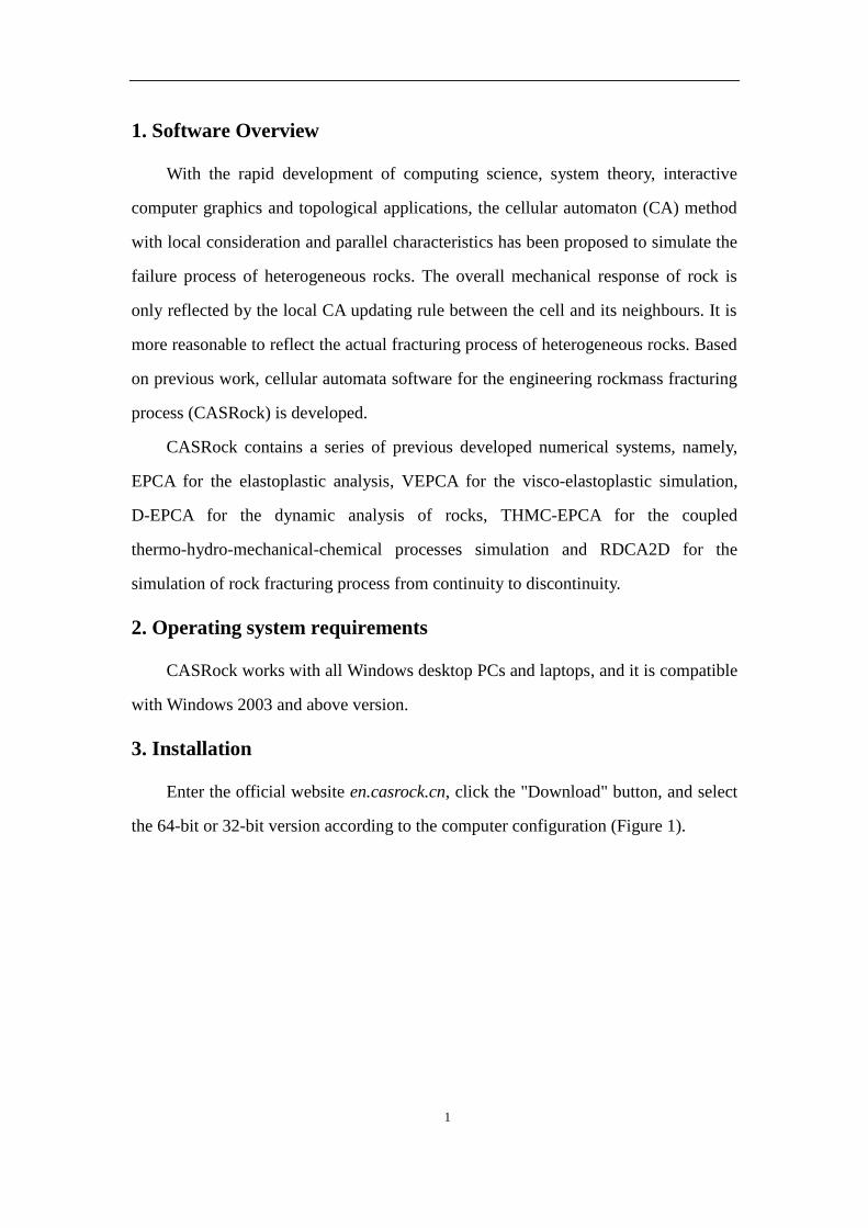
4.4.5 Section

The section dialog is shown in Figure 24.

16

Figure 24 Section

After setting the cut plane, turn off the contour image to display the actual cut

plane.

4.4.6 Sectioning

The sectioning dialog is shown in Figure 25.

Figure 25 Profile

Extract the boundary: remove the solid part of the 3D model and leave the model

boundary surface.

17

4.4.7 Element Plot

Display results in element display mode.

4.4.8 Animation Display

Read several result files, click animation display, set the starting and ending

calculation steps (Figure 26), and click preview to acquire the evolution process.

Click output AVI button to save.

Figure 26 Animation display

4.5 System Settings

4.5.1 Display settings

Set the background color, destroy color, contour font and size (Figure 27).

18

Figure 27 Display settings

4.5.2 Other settings

As shown in Figure 28, workspace directory, output setting, and language can be

set here.

Figure 28 Other settings

19

5. Menu bar

5.1 Home Page

5.1.1 Cell

1) Node mode: display results in the form of node interpolation;

2) Mesh plot: show or hide the grid;

3) Contour: show contour map of a certain variable;

4) Boundary Mesh: show or hide the model boundary;

5) CM variable: select the corresponding variable.

5.1.2 Element mode

1) Element mode: read the result with "Elem_contour" as the prefix and "econ" as

the suffix in“data”folder (Figure 29);

Figure 29 Element mode

2) Mode setting: set amplification factor of the result.

5.1.3 Material Mode

1) Material mode: different material categories can be displayed, as shown in Figure

30;

20

Figure 30 Material Mode

2) Material filter: Show or hide the material group corresponding to the material

number.

5.1.4 Page

This function takes effect when there are several data files.

1) First page: display the first one of the data file set;

2) Previous page: go to the previous one;

3) Next page: go to the next one;

4) Last page: display the last one of the data file set.

5.1.5 Camera

1) Rotation: three-dimensional rotation;

2) Rotate by X：rotation around the X-axis;

3) Rotate by Y：rotation around the Y-axis;

4) Rotate by Z：rotation around the Z-axis;

5) Translation: move the model;

6) Scaling: zoom the model;

7) Fit View: the model fills the view at the maximum scale;

8) XY plane: provide front view;

21

9) XZ plane: provide right view;

10) YZ plane: provide top view;

11) Isometric: provide axis side view ;

12) Camera: Record current view set;

13) Resetting: Restore to the recorded view set.

5.2 Function

5.2.1 Color table

1) Color Map: adjust the color of the legend, as shown in Figure 31;

2) Modify: add, delete and other operations to the color table;

3) Display setting: adjust the color table position, style, format, and precision.

Figure 31 The System of Color Table

4) Display color table: display or hide the color table;

5) Horizontal display: the color table is placed horizontally;

6) Vertical display: the color table is placed vertically;

7) Mesh Plot: show or hide color table boundaries;

8) Height / Width: adjust the color table size.

5.2.2 Display

1) Axis: display the coordinate system;

22

2) AE / MS: display the results of acoustic emission or micro- seismic balls;

3) Vector: display the result of a certain vector, such as displacement vector;

4) Contour line: display the contour line of contour image;

5) Section: display the cut plane;

6) Sectioning: display the profile.

5.2.3 Effect

1) Light: turn on or off the light;

2) Brightness: adjust the brightness;

3) Transparency: adjust the transparency.

5.2.4 Element display

Display element display results.

5.2.5 Other

1) Select node: acquire the information of the selected node;

2) Formula variables: combine existing variables with basic mathematical

operations for contour image output;

3) Displacement scaling: adjust the degree of displacement zoom.

5.3 Object

5.3.1 Anchor Bolt

1) Insert anchor bolt: insert bolt to the model;

2) AB Cloud Map: displays the bolt contour image.

5.3.2 Ball / Vector

1) AE / MS: display the results of acoustic emission or micro-seismic balls;

2) Vector: display a certain vector result.

23

5.3.4 Graphical annotation

1) Text box: insert a text box;

2) ChildWindow: Insert a sub-window.

5.4 Output

5.4.1 Animation output

Select several result files and output AVI video files.

5.4.2 Picture output

Select the result file and output the JPG image file.

5.4.3 Variable output

As shown in Figure 32, output data on a specified line or points.

Figure 32 Output specified point data

6. Typical cases

In the installation directory (" ...\CASRock\data\preprocessing\sample mesh

model "), several mesh grids of typical cases are provided, which can be directly

imported into the software (Figure 33).

24

Figure 33 Mesh grid

6.1 2D failure process of rocks under uniaxial compression

Simulating procedures :

(1) Set the working directory (e.g., D: \ CASRock \ 0.1-0.05-2d);

(2) Import the model grid file (0.1-0.05-2d.txt);

(3) Define the material parameters (Figure 34);

(4) Define the analysis type (Figure 35);

(5) Set the loading control method for general mechanical problems (Figure 36);

(6) Set the calculation and output control (Figure 37);

(7) Start calculation.

Read the result file (Figure 38) and display the variable contour graph (Figure 39)

in CASRock.

25

Figure 34 Material definition

Figure 35 Definition of analysis type

Figure 36 Uniaxial loading control

Figure 37 Calculation and output control

26

Figure 38 Read the result file of node display mode

Figure 39 Variable contour graph

6.2 3D failure process of rocks under true triaxial compression

Simulating procedures:

27

(1) Set the working directory (e.g., D: \ CASRock \ 3d-2000);

(2) Import the model grid file (3d-2000.txt, Figure 33);

(3) Define the material parameter (Figure 40);


(5) Set the loading control method for general mechanical problems (Figure 42);

(6) Set calculation and output control (Figure 43) ;


After calculation, the variable contour graph of node display mode (Figure 44)

and element display mode (Figure 45) can be acquired.



28

Figure 42 True triaxial loading control


Figure 44 Variable contour of node display mode result

Figure 45 Variable contour of element display mode result

29

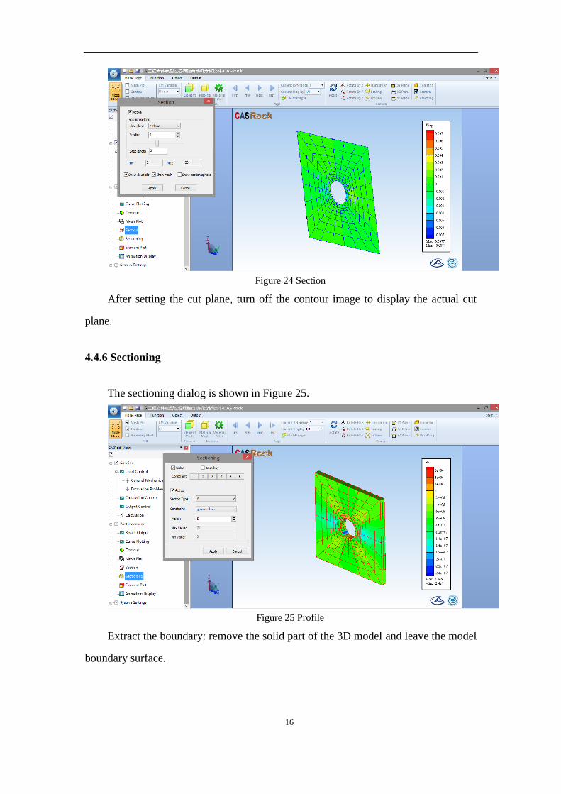
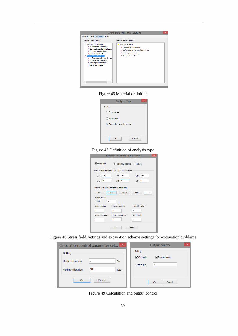
6.3 Excavation process of rockmass

Simulating procedures:

(1) Set the working directory (e.g., D: \ CASRock \ jp-3d);

(2) Import the model grid file (jp-3d.txt, Figure 33);

(3) Define the material parameter (Figure 46):


(5) Set loading condition for excavation problems, including stress condition

settings and excavation scheme settings (Figure 48);

(6) Set calculation and output control (Figure 49);


After calculation, contour graphs of displacement can be acquired in CASRock

(Figure 50).

30



Figure 48 Stress field settings and excavation scheme settings for excavation problems


31

Step 1 Step 2

Step 3 Step 4

Step 5

Figure 50 Displacement contour image during excavation

cellular automata software for engineering rockmass

Documents