cellular biophysics software based on matlab · cellular biophysics software based on matlab ......
TRANSCRIPT
CELLULAR BIOPHYSICS
SOFTWARE BASED ON MATLAB
Thomas Fischer Weiss
and Tanmaya Shubham Bhatnagar
Department of Electrical Engineering and Computer Science Massachusetts Institute of Technology
Fall 1997
Date of last modification: October 25, 1997

ii

iii
Preface
Historical perspective
During the 1980’s the use of computers and information technologies began to have an impact on higher education (Kulik and Kulik, 1986; Balestri, 1988; Wilson and Redish, 1989; Athena, 1990a; Athena, 1990b). As an integral part of this trend, in 1983 MIT in partnership with the Digital Equipment Corporation and the IBM Corporation launched Project Athena which was designed to make computation available to undergraduate students through a network of computers located in public clusters on the MIT campus (Athena, 1990a; Athena, 1990b). A major objective of Project Athena was to improve undergraduate education through the use of computation and information technologies. Faculty were encouraged to participate, and support for faculty software developers was provided on a competitive basis.
One of us (TFW) has been involved in teaching cellular biophysics at MIT since the 1960’s. The possibility of using software as a pedagogical aid was intriguing. With support from Project Athena, a software package on the Hodgkin-Huxley model for nerve excitation was developed as part of an undergraduate thesis (by David Huang), and was first used to teach cellular biophysics in the Fall 1984 semester. The software was designed to be easy to use so that a student’s attention would be focussed on the Hodgkin-Huxley model and not on the computer. Informal discussions with students and a survey of student views showed that the software was an enormous success. During the first semester, the software was used primarily in lecture demonstrations and as the basis for student projects. Both pedagogic methods were found to be effective. The use of the software in lecture was very effective in motivating and engaging students. The student projects were effective in allowing students to pursue a research project of their choice with staff assistance. For many students this was their first experience with a research project. The use of these projects, developed in the first year, was so successful that it has been used ever since.
The initial results with the Hodgkin-Huxley software were so successful educationally, that several other software development projects involving student programmers were launched. In all, 5 software packages were developed and have been used every year to teach the subject. All of these packages were revised extensively in response to suggestions from students and staff. The original software runs on UNIX workstations under MIT’s Project Athena and is available to the MIT community on a network of about 1000 UNIX workstations located in public clusters on the MIT campus as well as in some living groups. All this software was written in C and XWindows and was based on a library of graphic user interface subroutines written by one of the students (Giancarlo Trevisan). The software has been used in lectures, in recitations held in an electronic classroom in which each student uses a workstation, in homework assignments, and in stu

iv
dent projects. Various modes of use of the software in teaching were developed and are described briefly elsewhere (Weiss et al., 1992) and more extensively in the last chapter of this manual. The software has become an integral part of the subject, and it is difficult to imagine teaching the subject without the software.
Several problems became apparent in the development and utilization of the software. First, it was very expensive, in time and in money, to develop the software with the software tools available in the late 1980’s. Much of the time was expended in the development of graphic user interfaces that make the software easy for the user but which are tedious for the programmers to specify. These graphic user interfaces had to be written in a low-level language (XWindows). When Project Athena ended in 1991 and the funds from corporate sponsors were no longer available to support the development of new software, this development slowed considerably. Second, maintenance of the software became a major headache. It became difficult for a single faculty member with research, teaching, and other academic commitments to maintain a library of software in the face of changes in the operating systems. Third, as word spread about the existence of the software, educators and students outside of MIT requested the software. These requests accelerated dramatically after one of the software packages entitled Hodgkin-Huxley Model won the 1990 EDUCOM/NCRIPTAL Higher Education Software award for Best Engineering Software. However, almost all of the requests came from students and faculty with access to Macintosh or PC computers and not to UNIX workstations. Thus, when these people were informed that the software ran only on UNIX workstations, they invariably lost interest. At the time the software was written, the computational power of workstations so exceeded that of personal computers (PCs) that it was simply not possible to provide the type of performance on PCs that was achieved on the workstations. Furthermore, MIT’s Project Athena was committed to a network of UNIX workstations. Thus, for both software and hardware considerations, it did not make sense to port the existing software to PCs. Furthermore, the high cost of software development and maintenance did not justify further development of educational software on UNIX workstations alone. Thus, the development of new software was terminated in 1991.
By 1995, a number of developments made it feasible to address the problems described above and to develop software for teaching cellular biophysics in a manner that would make it easier to maintain, easier to modify, and widely available. Thus, all the software was rewritten to operate under MATLAB, which is a software package produced by The MathWorks, Inc., for the following reasons:
MATLAB is a powerful interpretive computational and visualization soft• ware package with a large number of higher-level built-in functions. Thus, it is suitable for the development of educational software packages.
MATLAB is available for Macintosh computers running on MacOS, PCs run• ning Microsoft Windows, and UNIX workstations running XWindows. Thus,

v
MATLAB runs on all the platforms commonly found in academic settings. The vendor supports changes in MATLAB that are required as changes in computer platforms occur. With the use of software built on MATLAB, this major maintenance job is transferred from individual faculty members to the vendor who has both the financial incentive and expertise to maintain the vendor software.
Large improvements in performance of PCs have made the development of • computationally intensive educational software feasible on these platforms.
MATLAB has provided increasingly sophisticated tools for building graphic • user interfaces (GUIs). These GUIs are essential for building user-friendly educational software packages.
MATLAB has rapidly become the de facto leader in supporting educational • computational subjects at MIT and elsewhere. Thus, students are exposed to MATLAB in other subjects and the different exposures are mutually reinforcing.
The effort to port the software to MATLAB was supported for 3 years by the National Science Foundation. The present software manual describes this software. Although the software is not linked directly to any textbook, it was developed in parallel with textbooks in cellular biophysics (Weiss, 1996a; Weiss, 1996b).
Acknowledgement
A number of people contributed to the success of the development of this software. We thank Project Athena, especially its two directors Steven Lerman and Earll Murman, for their support. In addition Gerald Wilson, Joel Moses, Richard Adler, Paul Penfield, and Jeffrey Shapiro were unfailingly supportive of this effort. A number of students were involved in this effort. David Huang wrote the first version of the Hodgkin-Huxley model package. David Koehler also contributed to this package. Devang M. Shah wrote the first version of the random-walk model package which was also revised by Elana B. Doering. Chapter 2 is based heavily on Devang’s thesis (Shah, 1990). Scott I. Berkenblit wrote the first version of the macroscopic diffusion package. Chapter 3 is based heavily on Scott’s thesis (Berkenblit, 1990). Stephanie Peek and Leela Obilichetti helped to develop the carrier-mediated transport package. Giancarlo Trevisan was a major contributor to all the packages. He wrote the first version of the voltage-gated ion channel package. He later rewrote the Hodgkin-Huxley package and the carrier-mediated transport package. He wrote all the graphic user interface routines that were ultimately used by all the packages. Generations of students benefited from his efforts. The recipients of the 1990 EDUCOM/NCRIPTAL Higher Education Software Award for Best Engineering Software for the Hodgkin-Huxley package were

vi
Thomas Weiss, Giancarlo Trevisan, and David Huang. More than a dozen generations of the students who took the subject helped to find flaws in the software and made valuable suggestions for its improvements.
Besides the support from Project Athena, the development of the software was supported by the Howard Hughes Medical Institute for which we are grateful. TFW was supported in part by the Thomas and Gerd Perkins professorship. The porting of the software to MATLAB was supported by the National Science Foundation (NSF), Division of Undergraduate Education. We would particularly like to thank Dr. Herbert Levitan, Section Head of Course and Curriculum Development of NSF. Dr. Karen C. Cohen has been helpful in the evaluation of the software.
The division of labor on the present MATLAB-based software is as follows: The software was designed by both TSB and TFW but is based heavily on the previous software. The MATLAB code was written by TSB. Both TSB and TFW tested the software extensively. The manual was written primarily by TFW.

Contents
1 INTRODUCTION 11.1 Overview Of Software Packages . . . . . . . . . . . . . . . . . . . . . . . 1 1.2 Brief Introduction To MATLAB . . . . . . . . . . . . . . . . . . . . . . . 2
1.2.1 Jargon . . . . . . . . . . . . . . . . . . . . . . . . . . . . . . . . . . 2 1.2.2 Help . . . . . . . . . . . . . . . . . . . . . . . . . . . . . . . . . . . 4
1.3 Starting And Quitting The Software . . . . . . . . . . . . . . . . . . . . 4 1.3.1 Directory structure . . . . . . . . . . . . . . . . . . . . . . . . . . 4 1.3.2 Starting the software . . . . . . . . . . . . . . . . . . . . . . . . . 4 1.3.3 Quitting the software . . . . . . . . . . . . . . . . . . . . . . . . . 7
1.4 Common Features Of Software Packages . . . . . . . . . . . . . . . . . 7 1.4.1 Controls . . . . . . . . . . . . . . . . . . . . . . . . . . . . . . . . . 7 1.4.2 Quitting a package . . . . . . . . . . . . . . . . . . . . . . . . . . 7 1.4.3 Printing/saving a figure . . . . . . . . . . . . . . . . . . . . . . . 8 1.4.4 Reading from and saving to a file . . . . . . . . . . . . . . . . . 8 1.4.5 Flexible graphic resource . . . . . . . . . . . . . . . . . . . . . . 8 1.4.6 Scripts . . . . . . . . . . . . . . . . . . . . . . . . . . . . . . . . . . 12
2 RANDOM WALK MODEL OF DIFFUSION 152.1 Introduction . . . . . . . . . . . . . . . . . . . . . . . . . . . . . . . . . . . 16
2.1.1 Historical background . . . . . . . . . . . . . . . . . . . . . . . . 16 2.1.2 Macroscopic and microscopic models . . . . . . . . . . . . . . . 16 2.1.3 Overview of software . . . . . . . . . . . . . . . . . . . . . . . . . 17
2.2 Description Of The Random-Walk Model . . . . . . . . . . . . . . . . . 18 2.2.1 Particle parameters within a region . . . . . . . . . . . . . . . . 19 2.2.2 Boundary conditions . . . . . . . . . . . . . . . . . . . . . . . . . 21 2.2.3 Parameters that change the number of particles in the field . 232.2.4 Statistics . . . . . . . . . . . . . . . . . . . . . . . . . . . . . . . . . 24
2.3 User’s Guide To The Software . . . . . . . . . . . . . . . . . . . . . . . . 25 2.3.1 RW controls . . . . . . . . . . . . . . . . . . . . . . . . . . . . . . . 26 2.3.2 Parameters . . . . . . . . . . . . . . . . . . . . . . . . . . . . . . . 26 2.3.3 Particles . . . . . . . . . . . . . . . . . . . . . . . . . . . . . . . . . 28 2.3.4 Histogram . . . . . . . . . . . . . . . . . . . . . . . . . . . . . . . . 29 2.3.5 Graph . . . . . . . . . . . . . . . . . . . . . . . . . . . . . . . . . . 29
vii

viii CONTENTS
2.3.6 Summary . . . . . . . . . . . . . . . . . . . . . . . . . . . . . . . . 29 2.3.7 Miscellaneous issues . . . . . . . . . . . . . . . . . . . . . . . . . 31
2.4 Problems . . . . . . . . . . . . . . . . . . . . . . . . . . . . . . . . . . . . . 31
3 MACROSCOPIC DIFFUSION PROCESSES 373.1 Introduction . . . . . . . . . . . . . . . . . . . . . . . . . . . . . . . . . . . 38
3.1.1 Background . . . . . . . . . . . . . . . . . . . . . . . . . . . . . . . 38 3.1.2 Macroscopic model of diffusion . . . . . . . . . . . . . . . . . . 38 3.1.3 Overview of software . . . . . . . . . . . . . . . . . . . . . . . . . 39
3.2 Methods of Solution . . . . . . . . . . . . . . . . . . . . . . . . . . . . . . 41 3.2.1 Exact solutions . . . . . . . . . . . . . . . . . . . . . . . . . . . . . 42 3.2.2 Numerical Solutions . . . . . . . . . . . . . . . . . . . . . . . . . . 44 3.2.3 Summary . . . . . . . . . . . . . . . . . . . . . . . . . . . . . . . . 45
3.3 User’s Guide To The Software . . . . . . . . . . . . . . . . . . . . . . . . 45 3.3.1 MD controls . . . . . . . . . . . . . . . . . . . . . . . . . . . . . . . 45 3.3.2 Initial concentration profile . . . . . . . . . . . . . . . . . . . . . 46 3.3.3 Numerics . . . . . . . . . . . . . . . . . . . . . . . . . . . . . . . . 52 3.3.4 Analysis figures . . . . . . . . . . . . . . . . . . . . . . . . . . . . 53 3.3.5 Arbitrary concentration profiles . . . . . . . . . . . . . . . . . . 55
3.4 Problems . . . . . . . . . . . . . . . . . . . . . . . . . . . . . . . . . . . . . 56
4 CARRIER-MEDIATED TRANSPORT 614.1 Introduction . . . . . . . . . . . . . . . . . . . . . . . . . . . . . . . . . . . 62 4.2 Models . . . . . . . . . . . . . . . . . . . . . . . . . . . . . . . . . . . . . . 62
4.2.1 Steady-state behavior of a simple, four-state carrier that bindsone solute . . . . . . . . . . . . . . . . . . . . . . . . . . . . . . . . 63
4.2.2 Steady-state behavior of a simple, six-state carrier that bindstwo solutes . . . . . . . . . . . . . . . . . . . . . . . . . . . . . . . 65
4.2.3 Transient and steady-state behavior of a general, four-statecarrier that binds one solute . . . . . . . . . . . . . . . . . . . . 67
4.3 Numerical Methods . . . . . . . . . . . . . . . . . . . . . . . . . . . . . . 70 4.3.1 Numerical methods . . . . . . . . . . . . . . . . . . . . . . . . . . 70 4.3.2 Choice of numerical parameters . . . . . . . . . . . . . . . . . . 71
4.4 User’s Guide . . . . . . . . . . . . . . . . . . . . . . . . . . . . . . . . . . . 71 4.4.1 CMT controls . . . . . . . . . . . . . . . . . . . . . . . . . . . . . . 71 4.4.2 Model . . . . . . . . . . . . . . . . . . . . . . . . . . . . . . . . . . 72 4.4.3 Steady-state interactive analysis . . . . . . . . . . . . . . . . . . 76 4.4.4 Steady-state graphic analysis . . . . . . . . . . . . . . . . . . . . 77 4.4.5 Transient analysis . . . . . . . . . . . . . . . . . . . . . . . . . . . 79
4.5 Problems . . . . . . . . . . . . . . . . . . . . . . . . . . . . . . . . . . . . . 81
5 HODGKIN-HUXLEY MODEL 855.1 Introduction . . . . . . . . . . . . . . . . . . . . . . . . . . . . . . . . . . . 86
5.1.1 Background . . . . . . . . . . . . . . . . . . . . . . . . . . . . . . . 86

CONTENTS ix
5.1.2 Overview of the software . . . . . . . . . . . . . . . . . . . . . . 86 5.2 Description Of The Model . . . . . . . . . . . . . . . . . . . . . . . . . . 86
5.2.1 Voltage-clamp and current-clamp configurations . . . . . . . . 87 5.2.2 The membrane current density components . . . . . . . . . . 87 5.2.3 The membrane conductances . . . . . . . . . . . . . . . . . . . . 88 5.2.4 The activation and inactivation factors . . . . . . . . . . . . . . 88 5.2.5 The rate constants . . . . . . . . . . . . . . . . . . . . . . . . . . . 89 5.2.6 Time constants and equilibrium values of activation and in
activation factors . . . . . . . . . . . . . . . . . . . . . . . . . . . 89 5.3 Numerical Methods . . . . . . . . . . . . . . . . . . . . . . . . . . . . . . 90
5.3.1 Background . . . . . . . . . . . . . . . . . . . . . . . . . . . . . . . 90 5.3.2 Choice of integration step �t . . . . . . . . . . . . . . . . . . . . 90 5.3.3 Method for computing solutions . . . . . . . . . . . . . . . . . . 91
5.4 User’s Guide To The Software . . . . . . . . . . . . . . . . . . . . . . . . 92 5.4.1 Controls . . . . . . . . . . . . . . . . . . . . . . . . . . . . . . . . . 92 5.4.2 Setup . . . . . . . . . . . . . . . . . . . . . . . . . . . . . . . . . . . 93 5.4.3 Analysis . . . . . . . . . . . . . . . . . . . . . . . . . . . . . . . . . 102 5.4.4 Scripting . . . . . . . . . . . . . . . . . . . . . . . . . . . . . . . . . 108
5.5 Problems . . . . . . . . . . . . . . . . . . . . . . . . . . . . . . . . . . . . . 109 5.6 PROJECTS . . . . . . . . . . . . . . . . . . . . . . . . . . . . . . . . . . . . 115
5.6.1 Practical considerations in the choice of a topic . . . . . . . . 116 5.6.2 Choice of topics . . . . . . . . . . . . . . . . . . . . . . . . . . . . 116 5.6.3 The proposal . . . . . . . . . . . . . . . . . . . . . . . . . . . . . . 122 5.6.4 The computations . . . . . . . . . . . . . . . . . . . . . . . . . . . 122 5.6.5 The report . . . . . . . . . . . . . . . . . . . . . . . . . . . . . . . . 122
6 VOLTAGE-GATED ION CHANNELS 1256.1 Introduction . . . . . . . . . . . . . . . . . . . . . . . . . . . . . . . . . . . 126
6.1.1 Historical background . . . . . . . . . . . . . . . . . . . . . . . . 126 6.1.2 Overview of software . . . . . . . . . . . . . . . . . . . . . . . . . 126
6.2 Description Of The Model . . . . . . . . . . . . . . . . . . . . . . . . . . 127 6.3 Numerical Methods . . . . . . . . . . . . . . . . . . . . . . . . . . . . . . 130
6.3.1 Integration step . . . . . . . . . . . . . . . . . . . . . . . . . . . . 130 6.3.2 Initial conditions . . . . . . . . . . . . . . . . . . . . . . . . . . . . 131
6.4 User’s Guide . . . . . . . . . . . . . . . . . . . . . . . . . . . . . . . . . . . 131 6.4.1 Controls . . . . . . . . . . . . . . . . . . . . . . . . . . . . . . . . . 132 6.4.2 Channel parameters . . . . . . . . . . . . . . . . . . . . . . . . . . 132 6.4.3 Membrane potential . . . . . . . . . . . . . . . . . . . . . . . . . . 136 6.4.4 Numerics . . . . . . . . . . . . . . . . . . . . . . . . . . . . . . . . 136 6.4.5 Analysis . . . . . . . . . . . . . . . . . . . . . . . . . . . . . . . . . 137
6.5 Problems . . . . . . . . . . . . . . . . . . . . . . . . . . . . . . . . . . . . . 142

x CONTENTS

List of Figures
1.1 Softcell figure showing the available software packages . . . . . . . . 5 1.2 The print figure . . . . . . . . . . . . . . . . . . . . . . . . . . . . . . . . 8 1.3 Example of the use of the flexible graphic resource . . . . . . . . . . 9 1.4 The select x,y figure . . . . . . . . . . . . . . . . . . . . . . . . . . . . . . 10 1.5 The axis scale figure . . . . . . . . . . . . . . . . . . . . . . . . . . . . . . 11
2.1 Definition of grid of particle locations . . . . . . . . . . . . . . . . . . 18 2.2 Definition of simulation field, regions, and boundaries . . . . . . . . 19 2.3 Motion of a particle in a homogeneous region . . . . . . . . . . . . . . 20 2.4 Motion of a particle at a vertical perimeter boundary . . . . . . . . . 22 2.5 Motion of a particle at an internal vertical boundary . . . . . . . . . . 23 2.6 The rw controls figure . . . . . . . . . . . . . . . . . . . . . . . . . . . . 26 2.7 Parameters figure . . . . . . . . . . . . . . . . . . . . . . . . . . . . . . . 27 2.8 Initial locations of particles . . . . . . . . . . . . . . . . . . . . . . . . . 28 2.9 Locations of particles after a 100 step random walk . . . . . . . . . . 29 2.10 Histogram of particle locations after a 100 step random walk . . . . 30 2.11 Standard deviation of particle location versus step number . . . . . 30 2.12 Numerical summary of statistics after a 100 step random walk . . . 302.13 Parameters for a random walk in 3 regions . . . . . . . . . . . . . . . 34 2.14 Initial locations of particles for a random walk in 3 regions . . . . . 35
3.1 Classes of initial concentration profiles simulated by the software . 403.2 The MD controls figure . . . . . . . . . . . . . . . . . . . . . . . . . . . . 46 3.3 Initial concentration figure for impulses . . . . . . . . . . . . . . . . . 47 3.4 Initial concentration figure for sinusoids . . . . . . . . . . . . . . . . . 48 3.5 Initial concentration figure for discontinuities . . . . . . . . . . . . . 49 3.6 Initial concentration figure using the arbitrary option . . . . . . . . . 50 3.7 Initial concentration figure for the two compartments option . . . . 51 3.8 The diffusion parameters figure . . . . . . . . . . . . . . . . . . . . . . 52 3.9 The numerics figure . . . . . . . . . . . . . . . . . . . . . . . . . . . . . . 53 3.10 Plots versus position figure . . . . . . . . . . . . . . . . . . . . . . . . . 54 3.11 Plots versus time figure . . . . . . . . . . . . . . . . . . . . . . . . . . . . 54
4.1 Kinetic diagram of the simple, four-state carrier . . . . . . . . . . . . 63 4.2 Kinetic diagram of a simple, six-state carrier that binds two solutes 65
xi

xii LIST OF FIGURES
4.3 Kinetic diagram of a general, four-state carrier model . . . . . . . . . 68 4.4 Controls figure . . . . . . . . . . . . . . . . . . . . . . . . . . . . . . . . . 72 4.5 Units of all variables in the carrier models . . . . . . . . . . . . . . . . 72 4.6 Parameters and state figures for the simple, four-state carrier model
that binds one solute . . . . . . . . . . . . . . . . . . . . . . . . . . . . . 73 4.7 Parameters and state figures for the simple, six-state carrier that
binds two solutes . . . . . . . . . . . . . . . . . . . . . . . . . . . . . . . 74 4.8 Parameters and state figures for the general, four-state carrier that
binds one solute . . . . . . . . . . . . . . . . . . . . . . . . . . . . . . . . 75 4.9 The steady-state graphic analysis figure . . . . . . . . . . . . . . . . . 78 4.10 The transient analysis figure . . . . . . . . . . . . . . . . . . . . . . . . 79 4.11 The set up transients figure . . . . . . . . . . . . . . . . . . . . . . . . . 80 4.12 The transient numerics figure . . . . . . . . . . . . . . . . . . . . . . . . 81
5.1 Voltage-clamp configuration . . . . . . . . . . . . . . . . . . . . . . . . . 87 5.2 Current-clamp configuration . . . . . . . . . . . . . . . . . . . . . . . . 87 5.3 The controls figure after the software is initiated . . . . . . . . . . . . 92 5.4 The controls figure after the software is initiated . . . . . . . . . . . . 93 5.5 The parameters versus membrane potential figure . . . . . . . . . . . 95 5.6 The select y figure . . . . . . . . . . . . . . . . . . . . . . . . . . . . . . . 95 5.7 Stimulus figure . . . . . . . . . . . . . . . . . . . . . . . . . . . . . . . . . 96 5.8 Example of a stimulus waveform . . . . . . . . . . . . . . . . . . . . . . 98 5.9 The numerics figure . . . . . . . . . . . . . . . . . . . . . . . . . . . . . . 98 5.10 The block diagram figure . . . . . . . . . . . . . . . . . . . . . . . . . . . 100 5.11 Expansion of the current clamped block . . . . . . . . . . . . . . . . . 100 5.12 The simulink figure . . . . . . . . . . . . . . . . . . . . . . . . . . . . . . 101 5.13 The sink figure . . . . . . . . . . . . . . . . . . . . . . . . . . . . . . . . . 101 5.14 Block diagram with oscilloscope attached . . . . . . . . . . . . . . . . 102 5.15 The oscilloscope screen . . . . . . . . . . . . . . . . . . . . . . . . . . . 103 5.16 The plot versus time figure . . . . . . . . . . . . . . . . . . . . . . . . . 103 5.17 The variable summary figure. . . . . . . . . . . . . . . . . . . . . . . . . 104 5.18 Comparison figure . . . . . . . . . . . . . . . . . . . . . . . . . . . . . . . 105 5.19 Phase-plane plot of membrane conductance versus membrane po
tential . . . . . . . . . . . . . . . . . . . . . . . . . . . . . . . . . . . . . . 106 5.20 Membrane potential obtained at different temperatures . . . . . . . 107 5.21 Simulation results for different parameters that block the action
potential . . . . . . . . . . . . . . . . . . . . . . . . . . . . . . . . . . . . . 114 5.22 Examples of action potentials . . . . . . . . . . . . . . . . . . . . . . . . 117 5.23 Dependence of the action potential on temperature . . . . . . . . . . 118 5.24 Effect of extracellular sodium concentration on the action potential 1185.25 Sample project proposal . . . . . . . . . . . . . . . . . . . . . . . . . . . 123
6.1 Kinetic diagram of a channel that has 5 states . . . . . . . . . . . . . 127 6.2 The probability of occurrence of more than 1 event in an interval �t 131
LIST OF FIGURES xiii
6.3 The controls figure after the software is initiated . . . . . . . . . . . . 132 6.4 The channel parameters figure . . . . . . . . . . . . . . . . . . . . . . . 133 6.5 Rate constant window . . . . . . . . . . . . . . . . . . . . . . . . . . . . . 134 6.6 View rate constant figure after both the forward and reverse rate
constants have been defined . . . . . . . . . . . . . . . . . . . . . . . . 135 6.7 Membrane potential figure . . . . . . . . . . . . . . . . . . . . . . . . . . 136 6.8 Numerics figure . . . . . . . . . . . . . . . . . . . . . . . . . . . . . . . . 136 6.9 State occupancy figure . . . . . . . . . . . . . . . . . . . . . . . . . . . . 138 6.10 Single channel ionic current . . . . . . . . . . . . . . . . . . . . . . . . . 139 6.11 Summary figure . . . . . . . . . . . . . . . . . . . . . . . . . . . . . . . . 140 6.12 Comparison figure . . . . . . . . . . . . . . . . . . . . . . . . . . . . . . . 141

xiv LIST OF FIGURES

List of Tables
2.1 The macroscopic laws of diffusion . . . . . . . . . . . . . . . . . . . . . 16
3.1 Summary of computational methods. . . . . . . . . . . . . . . . . . . 45
4.1 Modifiable parameters of the carrier models . . . . . . . . . . . . . . . 76
xv

xvi LIST OF TABLES

Chapter 1
INTRODUCTION
1.1 Overview Of Software Packages
The software for cellular biophysics consists of 5 software packages. The titles of the software packages, with acronyms in parentheses and brief descriptions, are:
Random Walk Model of Diffusion (RW) allows users to select parameters of the random walks of particles in a field and to observe the resulting space-time evolution of particle location. This package is intended to link the macroscopic laws of diffusion to its probabilistic, microscopic basis.
Macroscopic Diffusion Processes (MD) allows users to select the initial spatial distribution of solute concentration, the diffusion parameters, and to observe the resulting space-time evolution of solute concentration and flux. This package is intended to give users intuition about macroscopic diffusion processes.
Carrier-Mediated Transport (CMT) allows users to examine simple models of carrier-mediated transport through cellular membranes. For each of three models, the user can change any parameter and can instantly see the effect on the state of the carrier-model. This interactive mode is intended to build intuition about these models. In addition, there is a graphic mode that allows display of steady-state and transient responses to changes in any parameter.
Hodgkin-Huxley Model (HH) allows users to change parameters of the Hodgkin-Huxley model of a space-clamped giant axon of a squid, and to perform simulation experiments in either the voltage-clamp or the current-clamp configuration. This package is built on a block-diagram language providing users a graphic access to the model.
Voltage-Gated Ion Channels (IC) allows users to design a voltage-gated ion channel. The user selects the number of states, the conductance and gating
1
2 CHAPTER 1. INTRODUCTION
charge associated with each state, and the voltage-dependence of state transition rates. The user can then perform simulation experiments on the channel.
These packages are all designed to enhance comprehension of topics in cellular biophysics by providing pedagogic tools that can be used as a basis for lecture demonstration, open-ended problems that lend themselves to classes held in an electronic classroom in which students have access to computers, homework problems, and research projects. Although independent of any textbook, this suite of software packages was developed in parallel with textbooks in cellular biophysics (Weiss, 1996a; Weiss, 1996b).
1.2 Brief Introduction To MATLAB
All the software packages are written in MATLAB/SIMULINK which is an interactive programming environment for numerical and symbolic computations and for visualization of computational results. MATLAB is especially effective in systems analysis and signal processing. Because MATLAB runs on all the major computer platforms, the cellular biophysics software operates on all the major platforms: PCs using Windows, Macintosh computers using MacOS, and Unix workstations. Both MATLAB (version 4.2c) and SIMULINK (version 1.3) are required to operate this software.1
The MATLAB environment is interpretive. That is, commands can be entered at a prompt and interpreted within the scope of a MATLAB session. Thus, computational results generated by a simulation are available to the user for further analysis. The software is designed to perform all the simulations with minimal typed commands. The graphical user interface allows navigation through the software using a sequence of mouse events (e.g., clicking the mouse, pulling down a menu, dragging the mouse).
Users of the software do not need to learn MATLAB to use the software. However, knowledge of MATLAB can enhance user’s usage of the software. A number of texts on MATLAB are available (Hanselman and Littlefield, 1996). In addition, MATLAB manuals can be ordered directly from MathWorks. Section 1.2.1 is a glossary of some useful terms in the MATLAB vocabulary. Section 1.2.2 mentions resources that can provide on-line help with MATLAB.
1.2.1 Jargon
The following terms are useful in navigating in the MATLAB environment.
1Although not tested extensively, RW, MD, CMT, and IC run on the Student Version of MATLAB. However, it may be that parameters can be chosen for these packages which will not satisfy the limitations of the Student Version. HH requires SIMULINK in addition to MATLAB. However, currently HH does not run on the Student Versions of MATLAB plus SIMULINK.

3 1.2. BRIEF INTRODUCTION TO MATLAB
workspace A collection of variables in the current session of MATLAB. When MATLAB is started, the workspace is empty. Each software package defines its own variables and parameters which it adds to the workspace.
command window The window that appears when MATLAB is started. Commands entered at the MATLAB prompt (>>) in this window are evaluated in the workspace.
figure A rectangular window containing graphical objects, such as axes, buttons, and menu items. See the MATLAB command figure.
axes The area in a figure containing plots and annotation. See the MATLAB command axes.
buttons Rectangular regions allowing a sequence of commands to be executed when they are clicked, selected, or edited. See the MATLAB command uicontrol.
popup-menu A rectangular region showing the current popup-menu selection. When clicked, the menu is expanded to show all the options. See the MATLAB command uicontrol.
menubar A bar at the top of a figure (Windows and UNIX implementations) or at the top of the monitor screen (MacOS implementation) associated with the currently selected figure. When selected, the menu item expands to show its related submenu items. Submenu items marked with a check-mark are currently active selections.
M-file A text file containing a sequence of commands to be evaluated in the MATLAB workspace. The software contains a collection of m-files which can be recognized by the extension .m.
MAT-file A binary data file containing MATLAB variables. Each software package uses and stores a different set of variables.
parameters Numeric values that define each model.
variables Numeric values of independent variables set by the user or of dependent variables calculated from the model.
SIMULINK A block-diagram language that extends MATLAB’s capabilities to simulate dynamic systems.

4 CHAPTER 1. INTRODUCTION
1.2.2 Help
Help on MATLAB and SIMULINK is available through the command window usingthe following commands at the MATLAB prompt (>>)
who lists the variables in the current workspace.
help function provides some help on the command function.
help help provides help on getting started using help.
lookfor word finds functions that involve word.
Additional help is available in the descriptions of individual software packages.
1.3 Starting And Quitting The Software
1.3.1 Directory structure
The software is designed to be run from a directory that includes the following files/directories:
cmt is a directory that contains the carrier-mediated transport software.
hh is a directory that contains the Hodgkin-Huxley model software.
ic is a directory that contains the voltage-gated ion channel software.
md is a directory that contains the macroscopic diffusion processes software.
rw is a directory that contains the random walk model software.
softcell.m is a MATLAB m-file that initializes the software and allows the user to choose software packages from a menu.
tlib is a directory that contains a library of software routines used by all the packages.
1.3.2 Starting the software
The software is accessible through MATLAB/SIMULINK via a menu that allows selection of the software packages and initializes all packages. The startup procedure is given for the different platforms.

5 1.3. STARTING AND QUITTING THE SOFTWARE
Figure 1.1: Softcell figure showing the available software packages.
UNIX workstation on Project Athena. From the dashboard at the top of the monitor select Courseware �≥Electrical Engineering and Computer Science �6.021J/6.521J Quantitative Physiology �≥
≥
New MATLAB SoftwareThis procedure displays the softcell figure shown in Figure 1.1. Clicking on any package, initializes that package and hides the softcell figure.
Windows, MacOS, UNIX, and other operating systems. Initialize MATLAB, and type the following instruction (in the MATLAB window) at the MATLAB prompt (>>) >> cd directory where directory is the name of the directory (folder) that houses the cellular biophysics software.2 Then type >> softcell This command displays the softcell figure shown in Figure 1.1. Clicking on any package, initializes that package and hides the softcell figure.
In addition, there are two m-files used by the software that may not be part of the standard distribution of MATLAB 4.2c.
ODE Suite. One feature of the packages (transient response for CMT) makes use of MATLAB’s ODE Suite (specifically, the ode solver ode15s), a collection of algorithms optimized for solving ordinary differential equations. To use transient response with CMT, it is imperative that the ODE Suite be on MATLAB’s search path. Use the following checklist to insure that the ODE Suite is accessible to the cellular biophysics software:
2To verify that the directory is the right one, either type pwd to indicate the name of the present directory or type ls to list the contents of the directory. It should contain the file softcell.m. If it does not contain this file then either the selected directory is wrong or the cellular biophysics software is not installed on your computer.

6 CHAPTER 1. INTRODUCTION
1. At the MATLAB prompt, typewhich ode15s.
If MATLAB returns the name of a file, the ODE Suite is already installed; skip the rest of the checklist.
2. Check if the ODE Suite is resident in your computer. If the suite came with MATLAB, it is most likely in the directory (folder) hierarchy
matlab/toolbox/contrib. If you can find the file ode15s.m, skip to step 4.
3. Install a copy of the ODE Suite on your computer. You can download it from the MathWorks website at the URL
http://www.mathworks.com/ Place the new directory (folder) into contrib.
4. Append the folder which contains the ODE Suite to MATLAB’s search path. If the ODE Suite resides in
matlab/toolbox/contrib/ode, type the command
>> path(path,’matlab/toolbox/contrib/ode’);
[For a Windows/PC system the directory (folder) is specified by an address that looks like c:\matlab\toolbox\contrib\ode, whereas on MacOs, the directory (folder) is specified by an address that looks like MacHD:matlab:toolbox:contrib:ode.] For the remainder of the session, MATLAB will look through the folder matlab/toolbox/contrib/ode when searching for files from the ODE Suite. To make this change permanent, see MATLAB documentation on setting the default MATLAB search path.
Printing. All the packages make use of an m-file (printdlg.m) for printing. Use the following check list to insure that printdlg.m is accessible to the software.
1. At the MATLAB prompt, typewhich printdlg.
If MATLAB returns the name of a file, printdlg.m is already installed; skip the rest of the checklist.
2. The m-file printdlg.m is distributed in a folder called uitools. Check if uitools is resident in your computer. If the uitools came with MATLAB, it is most likely in the directory (folder) hierarchy
matlab/toolbox/uitools. If you can find the file printdlg.m, skip to step 4.
3. Install a copy of the uitools folder on your computer. You can download it from the MathWorks website or their ftp site which can be reached through their web site:

1.4. COMMON FEATURES OF SOFTWARE PACKAGES 7
ftp://ftp.mathworks.com/pub/mathworks/toolbox/uitools .
Place the new directory (folder) into toolbox.
4. Append the folder which contains the uitools folder to MATLAB’s search path, i.e., type the command
>> path(path,’matlab/toolbox/uitools’);
1.3.3 Quitting the software
Quitting any package displays the softcell figure again. To quit MATLAB, click on QUIT in the menubar and select Exit MATLAB. The menubar is located at the top of the figure in UNIX and Windows implementations and at the top of the monitor screen in the MacOS implementation.
1.4 Common Features Of Software Packages
Certain features are common to all the software packages and these are described here. When any of the software packages is selected in the softcell figure, one or more windows is displayed on the screen. MATLAB refers to these as figures.
1.4.1 Controls
Each package has a controls figure that allows the user to control the package. Although individual packages have different controls figures, all controls figures contain a log panel and a message panel. The log panel contains options for recording log entries of the session. Log entries are records of actions of the user during the simulation session. Clicking on Select file displays a window that allows choosing the name of the log file into which the log entries will be saved. The log entries can also be displayed in the message panel. In general, the message panel is used to send messages to the user.
1.4.2 Quitting a package
Each figure associated with each package contains a menubar. The menubar occurs at the top of the figure in UNIX and Windows implementations and at the top of the screen in Macintosh versions of the software. This menubar enables the user to quit the software package by clicking on XX and then selecting quit XX, where XX is the acronym for the package (e.g., CMT for carrier-mediated transport).

8 CHAPTER 1. INTRODUCTION
Figure 1.2: The print figure after Print was selected in the RW package (Particles #1 figure).
1.4.3 Printing/saving a figure
The menubar for each figure associated with each package also contains Print which if selected brings up the print figure (Figure 1.2). The user can either print the figure to the default printer, print to any printer by editing Device Option (to see how to do it type help print at the MATLAB prompt), or store a postscript file of the figure.
1.4.4 Reading from and saving to a file
A variety of information about the software can be saved in MAT-files using the standard MATLAB binary file format (see MATLAB’s save and load commands). For example, all the packages allow storage of simulation parameters to allow a simulation to be repeated at a later time. In addition, results of simulations can also be saved in files for later retrieval. However, the information stored varies for different software packages, and the individual descriptions of the packages should be consulted for more detailed information.
To restore state variables from a prior simulation, use Read parameters push-buttons which are found on some of the figures of all of the packages. Although data can be restored using load from the command-line, this method will not, in general, restore all relevant state variables necessary to run the software.
1.4.5 Flexible graphic resource
A flexible graphics resource is used by all the software packages to compare results of simulations. This resource is customized for each software package but contains features that are common to all the software packages and these are described in detail here. We illustrate the usage of this resource with examples from the carrier-mediated transport package. Selection of graphic analysis in the controls figure of the carrier-mediated transport package results in the display of the steady-state graphic analysis figure (Figure 1.3). This is a typical usage of the graphic resource. This figure contains a number of panels.
Plot control. The panel in the upper left corner controls plotting in the manner described below.

9 1.4. COMMON FEATURES OF SOFTWARE PACKAGES
Figure 1.3: An example of the use of the flexible graphic resource in the CMT package. The steady-state graphic analysis figure shows a plot of fluxes and carrier densities
iversus the inside concentration of solute S, cS , in linear ordinate and abscissa scales.

10 CHAPTER 1. INTRODUCTION
Figure 1.4: The select x,y figure that produced the plot shown in Figure 1.3. Note that ci (which is S highlighted in blue) was selected as the independent variable that defines the abscissa (horizontal axis) in the plot. The variables �E , �ES , nE
i , no E ,
nES , and noi ES were selected as the dependent vari
ables and plotted as the ordinates (vertical axis).
Select x,y. Clicking on this entry results in the display of the Select x,y figure (Figure 1.4) which allows selection of one independent variable which determines the abscissa of the plot and multiple dependent variables which determine the ordinates. Clicking on an independent variable selects it for the abscissa variable and deselects a previously selected variable. Clicking on an unselected dependent variable adds it to the collection of selected variables. Clicking on a selected dependent variable deselects it. A maximum of four types of dependent variables can be selected for plotting. In some packages (CMT), the range of the independent variable is selected in this figure.
Select data files. Clicking on this entry displays a figure that allows selection of a file from which previously stored parameters can be read. The types of data that are read varies with each package.
Graph x,y. Clicking on this entry results in a plot of the selected data.
Overlay. When this button is activated, the next set of plots are overlayed over the current set. When this option is not checked, the following plots replace the current ones.
Use data files. When this button is activated, the next set of plots are derived from the selected data files.
Save results. Clicking this button displays a figure that allows selection of a file into which the current data can be stored. The types of data that are stored varies with each package.
Clear. Clicking this button clears the plot area as well as the legend and cross-hair information.

11 1.4. COMMON FEATURES OF SOFTWARE PACKAGES
Figure 1.5: The axis scale figure after the abscissa was selected in Figure 1.3.
Axes control. The lowest panel in the figure shows the selected plots. The axes can be changed by clicking on either the ordinate or the abscissa variable which results in the display of the axis scale figure (Figure 1.5). The axis scale can be chosen to be linear, logarithmic, and/or reciprocal. If none of the options is chosen, the scale is linear. If log scale is chosen, the scale is logarithmic. If invert is chosen (available only in CMT) then the reciprocal of the abscissa variable is plotted either on a linear or on a logarithmic scale. In logarithmic coordinates, negative values of a variable (i.e., the fluxes) are truncated. Clicking on done hides the figure.
Legend. The legend panel records a list of all data plotted. The following are recorded.
Time stamp. The time and date when the curves were generated are indicated. Clicking on the time stamp alternately displays and hides all the curves associated with this legend item.
Line and symbol type. The color, line style, and symbol type are used to encode a particular variable; this marker is shown in the legend.
Variable name. The name of the variable that was plotted is shown. Clicking on the variable name alternately displays and hides the curve associated with this entry. When variables are added or deleted, the axis is auto-scaled if that option is selected — it is selected by default — in the axis figure.
Cross-line value. When the cross line is used, the value of all variables at a particular value of the independent variable is displayed. These values are accurate only when cross line is selected in the mouse-event controls panel (see below).
Message window. Messages to the user are displayed in the message window.

12 CHAPTER 1. INTRODUCTION
Mouse-event controls. The plot can be modified or queried in several ways.
Annotate. Click on annotate and then click on a desired location in the plot area. A text edit box appears at that location. Type the annotation in the text edit box and type <RETURN> when the annotation is completed. Clicking on the annotation and dragging the mouse moves the annotation to a desired location in the plot field. Clicking on clear removes the annotation.
Cross hair. Clicking on cross hair places a mouse-controlled cross hair in the plot field. Clicking the mouse at some location in the plot field places (in the cross-hair panel) the values of all variables at the location of the cursor. Clicking on hide removes the cross-hair values.
Cross line. Clicking on cross line displays a vertical line, the cross line, in the plot field at the location of the pointer cursor. The line follows the cursor as it moves across the plot field. The values of all plotted variables at the intersection with the cross line are displayed in the legend. The value of the independent variable is displayed above the legend. Clicking on reset removes the cross-line values from the legend and clicking off cross line removes the cross line from the plotting field.
Zoom. Clicking on zoom allows the user to magnify a region of the plotting field. Clicking and dragging the mouse produces a rectangle in a portion of the plot field; the rectangle defines the region to be magnified. Additional magnification can be achieved by zooming again. Click unzoom to undo the effects of all prior zooms.
1.4.6 Scripts
Scripting commands alleviate the burden of being present while repetitive, time consuming simulations are computed.3 The set of commands available to the software user can be found by issuing the command help XXscr, where XX is the acronym for the package.
Scripting can also be used to create customized plots of variables. For example, in the Hodgkin-Huxley package, after running a simulation, the time dependance of the sodium conductance can be plotted on a separate figure using the following commands:
u_gna = hhscr(’get’,’G_Na’); %get the sodium conductance vector u_time = hhscr(’get’,’t’); %get the vector of sampled time values figure; %create a new figure plot(u_time,u_gna); %plot sodium conductance vs. time
3A sample script is given in the chapter on the Hodgkin-Huxley model.

13 1.4. COMMON FEATURES OF SOFTWARE PACKAGES
Once the values of these variables are so obtained, they can be manipulated, modified, and saved to files. It is important to practice safe-workspace-integrity techniques by creating names of variables that are similar to but different from those defined in the workspace. To see a list of variables in the workspace, type who. In general, prefix the names of your own variables with a set of characters such as u_. In this way, variables can be manipulated or plotted without danger of creating inconsistencies in the workspace.
Although the set of scripting commands in the various XXscr files is not exhaustive enough to allow operating all aspects of the software from the command-line, it is sufficient to carry out some of the time-consuming elements of the simulation. Furthermore, by issuing only sanctioned scripting commands from the MATLAB >> prompt, the user is assured that variables in the workspace will not be corrupted with inconsistencies.

14 CHAPTER 1. INTRODUCTION

Chapter 2
RANDOM WALK MODEL OF DIFFUSION
15
16 CHAPTER 2. RANDOM WALK MODEL OF DIFFUSION
2.1 Introduction
2.1.1 Historical background
A bolus of soluble material will gradually spread out in its solvent until a uniform solution results. This diffusion process must have been familiar to humans in antiquity. However, a mathematical description of these macroscopic changes in concentration was not available until the 1850s (Fick, 1855), and a microscopic or particle-level model, not until the turn of this century (Einstein, 1906).
Diffusion plays an important role in such a wide range of disciplines, that it is important for students of science and engineering to develop an understanding of the macroscopic laws of diffusion and their microscopic basis. We will review some important characteristics of the macroscopic laws of diffusion and their relation to random-walk models. A fuller treatment is available elsewhere (Weiss, 1996a).
2.1.2 Macroscopic and microscopic models
Macroscopic laws of diffusion
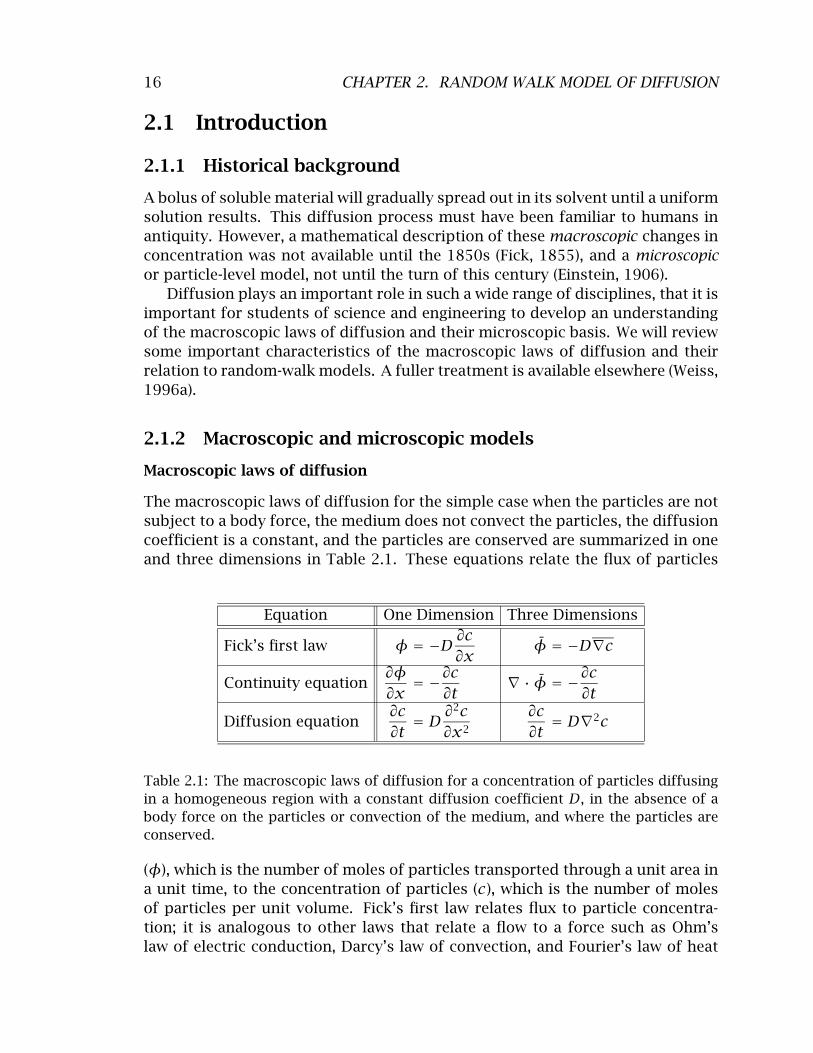
The macroscopic laws of diffusion for the simple case when the particles are not subject to a body force, the medium does not convect the particles, the diffusion coefficient is a constant, and the particles are conserved are summarized in one and three dimensions in Table 2.1. These equations relate the flux of particles
Equation One Dimension Three Dimensions
Fick’s first law � = −D θc
θx �̄ = −D∞c
Continuity equation θ�
θx = −
θc
θt ∞ · �̄ = −
θc
θt
Diffusion equation θc
θt = D
θ2c
θx2
θc
θt = D∞2c
Table 2.1: The macroscopic laws of diffusion for a concentration of particles diffusing in a homogeneous region with a constant diffusion coefficient D, in the absence of a body force on the particles or convection of the medium, and where the particles are conserved.
(�), which is the number of moles of particles transported through a unit area in a unit time, to the concentration of particles (c), which is the number of moles of particles per unit volume. Fick’s first law relates flux to particle concentration; it is analogous to other laws that relate a flow to a force such as Ohm’s law of electric conduction, Darcy’s law of convection, and Fourier’s law of heat

17 2.1. INTRODUCTION
flow. Fick’s first law implies that a solute concentration gradient causes a solute flux in a direction to reduce the concentration gradient. The continuity equation follows from conservation of particles, and the diffusion equation is obtained by combining Fick’s first law with the continuity equation.
Microscopic basis of diffusion
An important notion in understanding diffusion processes is to relate the macroscopic laws of diffusion to microscopic models of diffusing particles. The simplest microscopic model that captures the essence of diffusion is the discrete-time, discrete-space random walk. In a one-dimensional random walk in a homogeneous region of space, we assume a particle moves along the x-axis in a series of statistically independent steps of length +l or −l, where the time between steps is � . In an unbiased walk, positive and negative steps are equally likely, i.e., each has probability 1/2. It can be shown that statistical averages of properties of a population of particles obey the macroscopic laws of diffusion. In particular, this simple model can be shown (Weiss, 1996a) to yield Fick’s first law with a diffusion coefficient,
l2
D .2�
=
Therefore, the connection between the random walk of a particle and the laws of macroscopic diffusion can be made clear if the motion of a number of particles (on the order of 50) can be visualized for a number of steps.
2.1.3 Overview of software
The software described here is intended to allow users to investigate the properties of the simplest microscopic model that captures the essence of diffusion: the discrete-time, discrete-space random-walk model.
In the discrete-time, discrete space random walk model described here, there is a population of particles which execute statistically-independent, but otherwise identical two-dimensional random walks in a rectangular field. The field can be divided into one, two, or three homogeneous regions whose widths are specifiable, and whose properties may differ. Each particle undergoes a random walk with parameters that include: the probability that the particle takes a step to the left or right, and the step size. These parameters can be set independently in the three regions. The particles can be set to have a specifiable lifetime. One source and one sink of particles can be placed in the field and the initial concentration of particles can be specified in each of the three regions. Characteristics of the boundary conditions between regions can also be specified. With this software package it is possible: to visualize the spatial evolution of particle concentration from a variety of initial distributions selectable by the user; to examine the evolution of particle concentration from a source and in the presence of a sink;

18 CHAPTER 2. RANDOM WALK MODEL OF DIFFUSION
1 unit
j +2
j +1 Figure 2.1: Definition of grid of particle locations. A particle j is shown at the grid location (i, j). The distance between
j −1 adjacent grid locations, in both the horizontal and vertical directions, is the unit distance.
i −2
j −2
i −1 i i +1 i +2
to examine diffusion in regions of differing diffusion coefficients; to simulate diffusion of particles subjected to a body force; to simulate diffusion between two compartments separated by a membrane; to investigate the effects of chemical reactions or recombination which consume particles at a fixed rate; and to investigate the effects of different boundary conditions between regions. Two diffusion regimes can be run and displayed simultaneously to allow direct comparison between the space-time evolution of two different diffusion processes. In addition, a variety of statistics of the spatial distribution of particles can also be displayed.
By watching the particles move and by comparing simulation results to expectations, the user can develop an intuition for the way in which the random motions of particles lead to their diffusive spread.
2.2 Description Of The Random-Walk Model
In this simulation, the discrete-time, discrete-space random walk takes place on a finite two-dimensional grid of locations accessible to the particles and called the field. The location of each particle is specified by giving its coordinates on this grid (i, j) where i is the horizontal coordinate and ranges from 0 to 399 and j is the vertical coordinate and ranges from 0 to 99 (Figure 2.1). The horizontal distance between adjacent grid locations is 1 unit of distance and all spatial dimensions of the random walk are expressed as multiples of this unit distance. The location of the particle in the grid can change probabilistically at each step of the random walk. Thus, successive steps represent successive times that are separated by a unit time interval. All times are expressed in terms of the number of steps of the random walk.
The field can be divided into one, two or three homogeneous regions (Figure 2.2). Certain parameters of the simulation are defined for the entire field, others at boundaries between regions, and still others are defined independently for each region. The latter parameters will be described first and include: region size, particle step size, directional probabilities, and initial particle distribution.

19 2.2. DESCRIPTION OF THE RANDOM-WALK MODEL
Region 1 Region 2 Region 2
Region 1 size
vertical internal boundaries
perimeter boundary:
vertical horizontal
Figure 2.2: Definition of simulation field, regions, and boundaries. Solid lines delimit the perimeter boundaries of the field; dashed lines indicate the internal vertical boundaries that separate the regions.
2.2.1 Particle parameters within a region
The parameters that define the random walk are identical at each location within a region — each region is homogeneous. These parameters are described below.
Region size
The width of each region can be specified, but the sum of the widths cannot exceed 400. This allows a variety of diffusion regimes to be defined. For example, if Region 1 has width of 400 then the other two regions must have width 0 and the random walk is defined for one homogeneous region. By specifying two regions with non-zero widths, it is possible to define a diffusion process with different initial conditions in the two regions. This allows a rich variety of initial distributions to be defined. Three non-zero width regions allows simulation of diffusion between two regions separated by a third region with different properties. This might be used to investigate diffusion between two baths separated by a membrane.
Step size
The step size defines the distance, in multiples of unit distances, that particles may move in each step of time. Varying the step size simulates varying the diffusion coefficient. The size of a region is always set to a multiple of the step size in that region; all particles in a region are located at integer multiples of the step size starting from the left boundary of the region. This ensures that particles at a boundary fall on the boundary and simplifies the specification of particle motion at a boundary.

20 CHAPTER 2. RANDOM WALK MODEL OF DIFFUSION
upper left upper right
step size
expired
lower left lower right
step size
Figure 2.3: Schematic diagram of motion of a particle in a homogeneous region. The grid of possible particle locations, separated by unit distances, are indicated by + symbols. A particle is shown in the center of the figure at one instant in time. One time step later the particle either stays in the same location or moves to one of 4 possible locations (indicated by the shaded particle) or it expires (is removed from the field). If the particle moves, it translates one step size (here shown as 2 units of distance) in both the vertical and the horizontal direction.
Particle motion — directional probabilities
At each instant in time, a particle is at some location in the region. The disposition of the particle at the next instant in time is determined by one of six mutually exclusive and collectively exhaustive possibilities as illustrated in Figure 2.3. The particle can move one step size to the upper left, upper right, lower left, or lower right; stay in the same location (center); or be eliminated (expire). The probabilities for each of the six outcomes is as follows:
P[expired] 1/L , =
P[center] (1 − 1/L) (1 − p − q) , =
P[upper left] 0.5 (1 − 1/L)q ,=
P[upper right] 0.5 (1 − 1/L)p , (2.1)=
P[lower left] 0.5 (1 − 1/L)q ,=
P[lower right] 0.5 (1 − 1/L)p ,=
where L is the average lifetime of the particle, i.e. the average number of time steps to expiration; p is the conditional probability that the particle moves to the right given that it has not expired; q is the conditional probability that the particle moves to the left given that it has not expired. Note that while the probability of moving to the left and to the right can differ, the probability of moving up or down is always the same. Because the six probabilities define all the possible outcomes at each instant in time, they sum to unity.
Different types of random walks are described by changing the directional probabilities. The random walk defined by assuming p = q = 1/2 is the simple,

21 2.2. DESCRIPTION OF THE RANDOM-WALK MODEL
unbiased random walk described in Section 2.1. In general, if p = q the random walk is unbiased; there is no statistical tendency for particles to move preferentially in either horizontal direction. However, if p � q, the random walk is biased so that there is a tendency for particles to move in one horizontal direction. For a step size of S, the mean distance E[m] that the particle moves to the right in n units of time is
E[m] = Sn(1 − 1/L)(p − q) .
Initial distribution of particles
The initial distribution of particles can be specified in each of the three regions. Particles start at locations that are integral multiples of the step size in each region. Particles are distributed randomly (with a uniform distribution) in the vertical direction and have the selected distribution in the horizontal direction. The initial distribution of particles can be selected to be one of the following.
Empty implies that initially there are no particles in the region. •
Pulsatile implies that a specified number of particles are placed at a spec• ified horizontal location in the region and spaced randomly in the vertical direction.
Linear implies that a linear concentration profile is generated whose slope • and number of particles are specified. A uniform distribution of particles is obtained if the slope is set to zero. Negative concentrations are not allowed: if the parameters are chosen such that the concentration would become negative at some point in the region, these putative negative concentrations are set to zero.
Sinusoidal implies that the spatial distribution is sinusoidal with a specified • period and number of particles.
2.2.2 Boundary conditions
The field contains three different types of boundaries (Figure 2.2) which are, in order of increasing complexity, horizontal perimeter boundaries at the top and bottom of the field, vertical perimeter boundaries at the left and right ends of the field, and vertical internal boundaries that separate regions.
Horizontal perimeter boundaries
Horizontal perimeter boundaries act as perfectly reflecting walls. If a particle is located within one step size of such a boundary and takes a step toward the boundary then the new vertical location of the particle is determined in the following manner: the vertical distance the particle travels to reach the wall plus

22 CHAPTER 2. RANDOM WALK MODEL OF DIFFUSION
step size
upper right
lower right
expired
Figure 2.4: Schematic diagram of motion left vertical of a particle at a vertical perimeter bound-perimeter ary. For purposes of illustration the partiboundary
cle motion at the left boundary is shown. Conditions at the right boundary are the mirror-image of those shown here.
step size
the vertical distance the particle travels after reflecting from the wall must sum to the step size. This relation determines the new location given the old location and the value of the step size.
Vertical perimeter boundaries
The vertical perimeter boundaries are also reflecting walls. Because the probabilities of stepping to the left and right need not be the same, we found that purely reflecting wall of the type described for the horizontal perimeter boundaries created undesirable artefacts especially when the conditional probabilities of moving to the left and right were not equal (p � q). Therefore, we modified the boundary condition so that a particle that would have crossed a vertical perimeter boundary at a given step was placed on the boundary and then subject to the following boundary condition which is illustrated for the left boundary in Figure 2.4 and whose directional probabilities are:
P[expired] 1/L , =
P[center] (1 − 1/L) (1 − p) , (2.2)=
P[upper right] 0.5 (1 − 1/L)p ,=
P[lower right] 0.5 (1 − 1/L)p ,=
i.e. the particle cannot move to the left.
Vertical internal boundaries
The motion of particles at a vertical internal boundary is similar to that within a homogenous region. The differences are that: the step sizes in the two adjacent regions may differ; and special directional probabilities, specified by the user, apply at the boundary. These have been provided to allow users to explore the consequences of a rich variety of boundary conditions. To simplify boundary conditions, the software ensures that particles do not cross this boundary in one time step but rather they land on the boundary. This is guaranteed by forcing the width of boundaries, initial particle locations, locations of sources and sinks to be
23 2.2. DESCRIPTION OF THE RANDOM-WALK MODEL
step size inright region
step size inleft region
step size inright region
upper left
upper right
lower left
lower right
expired
left region right region
internal vertical boundary
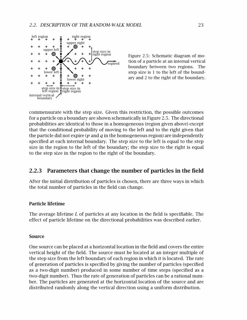
Figure 2.5: Schematic diagram of motion of a particle at an internal vertical boundary between two regions. The step size is 1 to the left of the boundary and 2 to the right of the boundary.
commensurate with the step size. Given this restriction, the possible outcomes for a particle on a boundary are shown schematically in Figure 2.5. The directional probabilities are identical to those in a homogeneous (region given above) except that the conditional probability of moving to the left and to the right given that the particle did not expire (p and q in the homogeneous region) are independently specified at each internal boundary. The step size to the left is equal to the step size in the region to the left of the boundary; the step size to the right is equal to the step size in the region to the right of the boundary.
2.2.3 Parameters that change the number of particles in the field
After the initial distribution of particles is chosen, there are three ways in which the total number of particles in the field can change.
Particle lifetime
The average lifetime L of particles at any location in the field is specifiable. The effect of particle lifetime on the directional probabilities was described earlier.
Source
One source can be placed at a horizontal location in the field and covers the entire vertical height of the field. The source must be located at an integer multiple of the step size from the left boundary of each region in which it is located. The rate of generation of particles is specified by giving the number of particles (specified as a two-digit number) produced in some number of time steps (specified as a two-digit number). Thus the rate of generation of particles can be a rational number. The particles are generated at the horizontal location of the source and are distributed randomly along the vertical direction using a uniform distribution.

24 CHAPTER 2. RANDOM WALK MODEL OF DIFFUSION
Sink
A sink can be placed at a horizontal location in the field and covers the entire vertical height of the field. The sink is located at an integer multiple of the step size from the left boundary of each region in which it is located. Particles that land on the sink are absorbed; hence the number of particles at the sink is always zero.
2.2.4 Statistics
Two sets of computations are performed simultaneously during a simulation: statistics based on the actual locations of particle and statistics based on the expected locations of particles. Given a particle location at one step and a set of directional probabilities, a random number generator is used to determine which of the possible new locations occurs at the next step. These sequence of locations determines the locations of the particles on the screen and all the statistics labelled actual. However, given a particle location at one time and the same directional probabilities, an expected location of the particle in the next step is also computed. Thus, during a simulation both the set of actual and expected locations for the particles are computed and can be displayed.
Histogram of horizontal particle locations
Histograms summarize the spatial distribution of particle locations. Each histogram consists of a set of bins that spans the field in the horizontal direction; the number of bins depends upon the specification of the bin size. With a bin size of 16, there are 25 bins that span the entire field of 400 locations. The histogram shows the number of particles in each bin as a function of bin location. Choice of bin size is important. A small bin size depicts the particle distribution with high spatial distribution. However, a small bin size implies that each bin will contain relatively few particles and the number of particles will fluctuate randomly from bin to bin. Conversely, a large bin size gives a histogram with poor spatial resolution but a larger amount of statistical averaging of the spatial distribution of particles.
The shape of the histogram is sensitive to the choice of bin size and can lead to confusing patterns. For example, suppose the bin size is five and the step size is two. Suppose further that particles are located uniformly in the field; one particle per accessible location. However, the step size constrains the possible locations that a particle may occupy to be separated by 2. Therefore, with a bin size of five, successive bins in the histogram alternate between 2 and 3 particles. Thus the histogram will not appear uniform, but oscillatory. This problem is cured if the bin size is an integral multiple of the step size. If the step sizes differ in the three regions, then the bin size should be set equal to the least common multiple of the three step sizes.

2.3. USER’S GUIDE TO THE SOFTWARE 25
Statistics as a function of step number
A number of statistics (both actual and expected) can be plotted versus step number. These are:
Mean is the mean location of the particles in the entire field. •
Standard Deviation is the standard deviation of particle location in the • entire field.
#Generated is the cumulative number of particles generated by the source • since the beginning of the simulation.
#Absorbed is the cumulative number of particles absorbed by the sink since • the beginning of the simulation.
#Expired is the cumulative number of particles lost (due to their finite life• times) since the beginning of the simulation.
Total #Particles is the total number of particles in the entire field at each • step number.
Region 1 #Particles is the total number of particles in Region 1 at each step • number.
Region 2 #Particles is the total number of particles in Region 2 at each step • number. For this total only, the particles located at the boundary between Region 1 and Region 2 are counted as belonging to Region 2.
Region 3 #Particles is the total number of particles in Region 3 at each step • number. For this total only, the particles located at the boundary between Region 2 and Region 3 are counted as belonging to Region 3.
These statistics allow a quantitative evaluation of simulation results. We give a number of examples of the use of these statistics. A systematic change in the mean location of the particles as a function of step number demonstrates a drift or migration of the particles as can be achieved by a bias in the directional probabilities. A difference in the standard deviation of two distributions can be achieved by changing the step size. The dependence on step number of the number of particles in the field, in a region, generated, absorbed, or expired can be used to assess whether a particle distribution has reached steady state. The change in the total number of particles in each region can be used to estimate the rate of transport of particles between regions.
2.3 User’s Guide To The Software
When this software package is selected, 3 figures are displayed (in addition to MATLAB’s command window) — RW Controls, Parameters #1, and Particles #1.

26 CHAPTER 2. RANDOM WALK MODEL OF DIFFUSION
Figure 2.6: The controls figure.
2.3.1 RW controls
The controls figure controls the random walk software and is shown in Figure 2.6. The part of the controls figure below the menubar is divided into four horizontal panels. The top panel indicates which aspects of the simulation(s) are to be displayed. Two independent simulations can be run simultaneously. The left-hand side contains the controls for Simulation #1 and the right-hand side for Simulation #2. Clicking on Histogram #1, for example, displays a histogram of particle locations for Simulation #1. Clicking on it again hides this histogram. These displays are described in detail below. The next panel down allows the simulation to be started, paused, continued, or stopped. The number of steps in the random walk before the simulation pauses can be entered in the text edit box. The end step indicates the current maximum value of the number of steps. This value is incremented if the simulation pauses and is continued. Clicking 1-step executes one step of the random walk. The third horizontal panel from the top is a message window that displays information to the user. The log panel contains options for recording log entries of the session and is described in Chapter 1. The bottom right panel allows reading parameters from a file and saving parameters to a file.
2.3.2 Parameters
The parameters figure is shown in Figure 2.7. The parameters figure allows selection of the parameters of the simulation(s). The parameters are given below.
Region Size. The user may define up to three regions, whose combined • width may not exceed 400. To eliminate a region, enter 0 for the region size. Regions can also be of size k(step − size) where k 3, 4, 5, .... That= is, regions of size stepsize and 2(stepsize) are not allowed.
27 2.3. USER’S GUIDE TO THE SOFTWARE
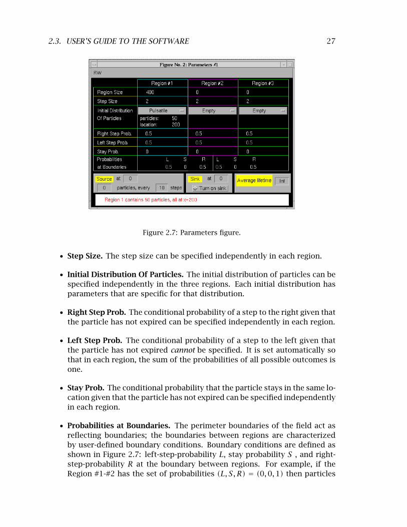
Figure 2.7: Parameters figure.
Step Size. The step size can be specified independently in each region. •
Initial Distribution Of Particles. The initial distribution of particles can be • specified independently in the three regions. Each initial distribution has parameters that are specific for that distribution.
Right Step Prob. The conditional probability of a step to the right given that • the particle has not expired can be specified independently in each region.
Left Step Prob. The conditional probability of a step to the left given that • the particle has not expired cannot be specified. It is set automatically so that in each region, the sum of the probabilities of all possible outcomes is one.
Stay Prob. The conditional probability that the particle stays in the same lo• cation given that the particle has not expired can be specified independently in each region.
Probabilities at Boundaries. The perimeter boundaries of the field act as • reflecting boundaries; the boundaries between regions are characterized by user-defined boundary conditions. Boundary conditions are defined as shown in Figure 2.7: left-step-probability L, stay probability S , and right-step-probability R at the boundary between regions. For example, if the Region #1-#2 has the set of probabilities (L, S, R) = (0, 0, 1) then particles
28 CHAPTER 2. RANDOM WALK MODEL OF DIFFUSION
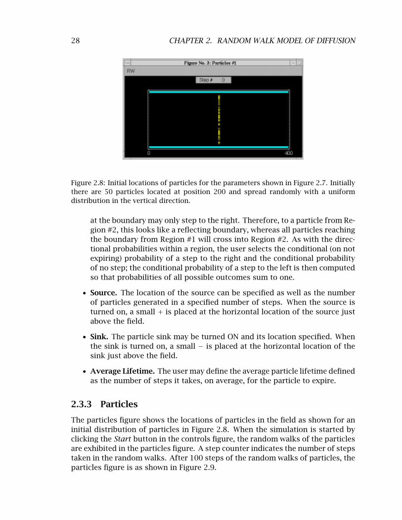
Figure 2.8: Initial locations of particles for the parameters shown in Figure 2.7. Initially there are 50 particles located at position 200 and spread randomly with a uniform distribution in the vertical direction.
at the boundary may only step to the right. Therefore, to a particle from Region #2, this looks like a reflecting boundary, whereas all particles reaching the boundary from Region #1 will cross into Region #2. As with the directional probabilities within a region, the user selects the conditional (on not expiring) probability of a step to the right and the conditional probability of no step; the conditional probability of a step to the left is then computed so that probabilities of all possible outcomes sum to one.
Source. The location of the source can be specified as well as the number • of particles generated in a specified number of steps. When the source is turned on, a small + is placed at the horizontal location of the source just above the field.
Sink. The particle sink may be turned ON and its location specified. When • the sink is turned on, a small − is placed at the horizontal location of the sink just above the field.
Average Lifetime. The user may define the average particle lifetime defined • as the number of steps it takes, on average, for the particle to expire.
2.3.3 Particles
The particles figure shows the locations of particles in the field as shown for an initial distribution of particles in Figure 2.8. When the simulation is started by clicking the Start button in the controls figure, the random walks of the particles are exhibited in the particles figure. A step counter indicates the number of steps taken in the random walks. After 100 steps of the random walks of particles, the particles figure is as shown in Figure 2.9.

29 2.3. USER’S GUIDE TO THE SOFTWARE
Figure 2.9: Locations of particles after a 100 step random walk for the same parameters as shown in Figure 2.7 and for the initial locations of particles shown in Figure 2.8.
2.3.4 Histogram
Selecting Histogram in the controls figure displays the histogram figure (Figure 2.10). The binwidth of the histogram can be selected in the upper right-hand corner. The binwidth determines the resolution of the histogram. Small bin widths produce histograms of particle locations with high spatial resolution but a great deal of statistical variation. Large bin widths result in histograms with poorer spatial resolution but less statistical variation in the histogram. The binwidth should be a multiple of the particle step size to avoid artefacts that result from incommensurate values. Clicking on the ordinate axis label displays an axis figure that allows the user to change the ordinate scale.
2.3.5 Graph
Selecting Graphs in the control figure displays the graphs figure. The temporal evolution of any of the statistics described in Section 2.2 can be plotted versus the step number. Figure 2.11 shows an example of the standard deviation of particle locations plotted versus step number. Clicking on the ordinate axis label displays an axis figure that allows the user to change the ordinate scale.
2.3.6 Summary
Numerical values of statistics can be displayed in the summary figure as shown in Figure 2.12

30 CHAPTER 2. RANDOM WALK MODEL OF DIFFUSION
Figure 2.10: Histogram of particle locations after a 100 step random walk for the same parameters as shown in Figure 2.7 and for the initial locations of particles shown in Figure 2.8. The histogram is for the particle locations shown in Figure 2.9.
Figure 2.11: Standard deviation of particle location versus step number for the same parameters as shown in Figure 2.7 and for the initial locations of particles shown in Figure 2.8.
Figure 2.12: Numerical summary of statistics after a 100 step random walk for the same parameters as shown in Figure 2.7 and for the initial locations of particles shown in Figure 2.8.

2.4. PROBLEMS 31
2.3.7 Miscellaneous issues
Time taken for random walks
All of the figures can be displayed simultaneously as the random walks are executed for two independent simulations. However, the display of each additional figure slows down the simulation. Increasing the number of particles also slows down the simulation.
Color coding of regions
Region #1 is indicated in blue in both the parameters figure and the particles figure; magenta is used for region #2 and green for region #3.
2.4 Problems
Problem 2.1 This problem deals with random walks of particles that begin from the same horizontal location.
a. Use the default simulation parameters with a pulsatile initial distribution of particles but set the step size to 2 and 4 for Simulations #1 and #2, respectively. Run the simulation for 100 steps. Note that the parameters of Simulation #1 and #2 differ only in step size. Examine graphs of the average and the standard deviation of the horizontal locations of the particles versus step number.
i. Explain quantitatively the differences in the graphs in terms of the difference in step size of the two simulations.
ii. Why does the slope of the standard deviation decrease with step number? What type of dependence on step number do you expect? Explain.
b. Now set the step size to 2 for both simulations and decrease the number of particles in the pulsatile initial distribution for one of the simulations to 25. Rerun the simulation. How does the number of particles affect the dependence of average location and standard deviation on step number?
c. Set all the parameters at their default values and then set the step size for both Simulation #1 and #2 to 2. For simulation #1 set the right step probability to 0.75, the left step probability to 0.25, place an impulse of 50 particles at location 100. For simulation #2 set the right step probability to 0.25, the left step probability to 0.75, place an impulse of 50 particles at location 300. Run the simulation for at least 100 steps. Examine graphs of the average and the standard deviation of the horizontal locations of the particles versus step number. Explain these results quantitatively.

32 CHAPTER 2. RANDOM WALK MODEL OF DIFFUSION
Problem 2.2 This problem deals with the steady-state distribution of particles in the presence of a source and sink for both unbiased and biased random walks. For all parts of this problem set the parameters for both Simulation #1 and #2 as follows: make the size of Region #1 400; the step size 20; and make the initial distribution of particles empty. Also place a source at location 0 and a sink at location 400 and make the histogram bin size 20.
a. Make the random walks for both Simulation #1 and #2 unbiased with a right step probability of 0.5. For simulation #1 make a source that generates 1 particle every 2 steps and for Simulation #2 make a source that generates 1 particle every 1 step. Make the particle lifetime infinite for both simulations. Now run the simulation. In the steady-state, by definition the particle distribution will not depend upon step number.
i. Before you run the simulation, estimate the form of the steady-state particle distribution. Is it uniform, exponential, pulsatile, linear, Gaussian, or none of these?
ii. Using the statistics available, determine a criterion for estimating when the particle distribution is in steady state.
iii. Now run the simulation until your criterion for steady state is met. What is the steady-state particle distribution? Does it fit with your initial expectation?
iv. How can you explain the difference in steady-state distribution for the two simulations?
v. Show that the steady-state particle distribution you have found for the random walks is consistent with Fick’s laws.
b. Use the same parameters for Simulation #2 as in part a, but change those of Simulation #1 so that the source rate is also 1 particle every 1 step; and so that the probability of a right step is 0.55. Run the simulation until it has reached a steady state.
i. Compare the steady-state distributions for the biased and unbiased random walks. How do they differ?
ii. What is the shape of the steady-state distribution for the biased walk?
iii. How would you modify Fick’s first law to account for not only diffusion of particles but a steady drift of particles of velocity v ? What steady-state distribution of particles is predicted from Fick’s laws and the continuity equation in the presence of this steady drift of particles? Is this consistent with the simulation results you obtained?
c. Keep the parameters of Simulation #1 and #2 the same as in part b, but change the right step probability of Simulation #2 to 0.48. Explain the differences in the shapes of the steady-state distributions for the two simulations.

33 2.4. PROBLEMS
Problem 2.3 This problem deals with the effect of a finite particle lifetime on the statistics of random walks.
a. Define a simulation with an initial particle distribution that is a uniform distribution of particles in space, but with a finite average particle lifetime. Run the simulation until all the particles have expired. Examine a graph of # particles versus step number. Explain the shape of this function.
b. Define another simulation that is identical with the one in part a, but this time with a source of particles. Do you expect a steady state to be reached between the the source and expirations? Determine a criterion for steady state and check out your intuition.
c. Design a combination of source rate and lifetime such that the distribution reaches a steady state. This might correspond, for example, to a drug concentration reaching steady state in the body, as it is both infused and eliminated.
d. Design a combination of source rate and lifetime such that most particles in the region have expired by the time the source injects the next batch. This might correspond to the drug concentration when the dosing interval is longer than the elimination half-life of the drug.
Problem 2.4 This problem deals with a random walk in three regions. Set up the parameters as shown in Figure 2.13. For both simulations, the two end regions contain uniform concentrations of particles; but the number of particles differs. There is a concentration difference between the end regions as shown in Figure 2.14 for one of the simulations; the other is similar. The center region can be regarded as a membrane that separates the two end regions and contains no particles initially. The random walk in the membrane region is unbiased in one simulation and biased in the other. Run the simulation for several hundred steps.
a. Explain the differences between the distributions of particles for the two simulations.
b. Quantitatively describe the flux of particles between the two end compartments — both the magnitude and sign of the flux.
c. What physical process might be represented in Simulation #2?
Problem 2.5 Design a three region diffusion regime where the center region is considered to be a membrane. Design membrane characteristics such that the membrane is transparent for particles moving from left to right but purely reflecting for particles moving from right to left. Test your design by running the simulation.

34 CHAPTER 2. RANDOM WALK MODEL OF DIFFUSION
Figure 2.13: Parameters for a random walk in 3 regions (Problem 2.4).

35 2.4. PROBLEMS
Figure 2.14: Initial locations of particles for a random walk in 3 regions (Problem 2.4).
Problem 2.6 Start with two identical simulations with Regions #1 and #2 that have: a region size of 400; a step size of 2; unbiased random walks; no sources or sinks; infinite particle lifetimes; and sinusoidal initial particle distributions. Choose one simulation with a period of 200 and the other with a period of 50. Choose an appropriate bin size for the histograms. Run the simulation.
a. What is the shape of the equilibrium distribution of particles?
b. Which particle distribution approaches this equilibrium faster?
c. Experiment with different frequencies and generalize your conclusion from part b.

36 CHAPTER 2. RANDOM WALK MODEL OF DIFFUSION

Chapter 3
MACROSCOPIC DIFFUSION PROCESSES
37

38 CHAPTER 3. MACROSCOPIC DIFFUSION PROCESSES
3.1 Introduction
3.1.1 Background
Diffusion is an important transport process in physical, chemical, and biological systems. Two theoretical models of diffusion capture complementary aspects of the phenomenon. The microscopic model describes the probabilistic behavior of a population of individual solute particles which execute statistically independent, but otherwise identical, random walks. Software dealing with such a microscopic model of diffusion is described in Chapter 2. The software described in this chapter involves macroscopic diffusion which describes the aggregate behavior of large populations of solute particles.
3.1.2 Macroscopic model of diffusion
In 1855, Adolph Fick proposed a macroscopic model for passive diffusion (Fick, 1855). By analogy to Fourier’s law of heat conduction and Ohm’s law for electrical conduction, Fick proposed that the flux of solute at a point in space is proportional to the concentration gradient at that point. Mathematically, this relation is expressed by Fick’s first law, which, in its one-dimensional form, is as follows:
θc (3.1)� = −D
θx,
where c(x, t) is the solute concentration and �(x, t) is the solute flux. The constant of proportionality, D, is known as the diffusion coefficient. Conservation of solute (in the absence of sources or sinks or of chemical reactions that create or destroy solute) results in a second relation between concentration and flux, the continuity equation:
θ� θc
θx = −
θt . (3.2)
Differentiating both sides of Equation 3.1 with respect to x and using the continuity equation yields Fick’s second law, or the one-dimensional diffusion equation:
θc θ2cD (3.3)
θt θx2=
In principle, any one-dimensional diffusion process can be modelled by solving this equation subject to the appropriate initial conditions and boundary conditions.
We next consider the same problem but with two changes: (1) a body force acts uniformly on the solute so that it drifts (migrates) and (2) a chemical reaction occurs that removes solute. The solute flux, �(x, t), is now the sum of the diffusive flux, given by Fick’s law, and the flux due to drift. Thus, in this case,
θc
θx + vc, (3.4)� = −D

39 3.1. INTRODUCTION
where v is the drift velocity of the solute; i.e., the velocity of the solute in response to the body force in the absence of diffusion. If r is the reaction rate at which solute is removed, then the continuity equation becomes
θ� θc
θt − rc. (3.5)
θx = −
Combining these expressions yields a modified diffusion equation:
θc θ2c θcDθx2
− vθx − rc. (3.6)
θt =
Thus, solute drift and a chemical reaction that removes solute contribute additional terms to the diffusion equation.
If the initial concentration, c(x, 0) is known in some region of space and if the relation between the concentration and flux is known at each boundary of this region, then a unique solution exists for t > 0. This agrees with intuition. Given an initial concentration profile, c(x, 0), Fick’s laws govern the unique evolution of the concentration profile for all later times.
3.1.3 Overview of software
While macroscopic diffusion has been successfully modelled by Fick’s equations, studying the equations alone provides only limited insight into the behavior of diffusion processes. The goal of this software is to help users gain intuition about diffusion in one dimension. The solutions to the diffusion equation are functions of two variables: one spatial variable, x, and time, t. These solutions can be plotted either as a function of time at a particular point in space or as a function of the spatial variable at a particular instant in time. Such isolated snapshots, however, do not fully convey the dynamic behavior of diffusion processes. With this software, the user can view a movie of the solute concentration or flux profile, as a function of position, as it evolves in time. Thus, the software enables the user to gain intuition about the dynamic behavior of macroscopic diffusion processes.
Furthermore, the software provides an opportunity for users to experiment with the macroscopic diffusion processes. For example, the user can explore how changing the diffusion coefficient affects the time-course of the simulation. The user can also specify transparent or reflecting boundaries and can explore how a body force acting on the solute or a chemical reaction that removes solute influence the diffusion process. Thus, the software can be used as a tool for investigating how various parameters and boundary conditions influence diffusion processes.
Five options for initial concentration profiles, corresponding to five characteristic diffusion problems, are implemented in the software (Figure 3.1). Four of these problems involve diffusion from a specified initial concentration profile in a one-dimensional region of space (which may be infinite in extent), while the fifth involves diffusion between two finite, well-mixed compartments separated by a membrane.

40 CHAPTER 3. MACROSCOPIC DIFFUSION PROCESSES
Bath 1 M Bath 2
Init
ial
con
cen
trat
ion
Impulse
Sinusoid
Discontinuity
Arbitrary
Two compartment
Figure 3.1: Schematic representation of the five classes of initial concentration profiles simulated by the software. M designates the membrane.
Position

3.2. METHODS OF SOLUTION 41
One-dimensional diffusion
In one-dimensional diffusion, the initial concentration can be chosen to be one of four options: impulses, sinusoids, discontinuities, and an arbitrary spatial distributions. An impulse of solute concentration is a mathematical idealization corresponding to a finite amount of solute initially concentrated at a single point in space. In the impulses option, the user can specify the magnitude and position of up to four impulses. This option illustrates diffusion from point sources. The sinusoids option illustrate the spatial frequency response of a system governed by the diffusion equation, specifically, the low-pass spatial filtering effect of diffusion. By superimposing up to four sinusoids, the user can observe the dependence of the space-time evolution of concentration on its spatial frequency content. In the discontinuities option, the initial concentration profile may be piecewise-constant but contain discontinuities. The user can specify the magnitude and location of up to four such discontinuities. For example, this allows simulation of the diffusion that results from an initial rectangular pulse of solute concentration. The user can also explore the response for more complicated initial conditions which can be specified by drawing an arbitrary initial concentration on the monitor screen with a mouse.
For these different initial distributions, the user can specify the boundary type (transparent or reflecting), the value of the drift velocity, and the chemical reaction rate at which solute is removed.
Two-compartment diffusion through a membrane
In the two compartment option, the user can also investigate diffusion between two well-stirred compartments, or baths, through a membrane which is permeable to the solute. Two-compartment diffusion through a membrane is an important transport process in biological systems. It can model, for example, diffusion between the cytoplasm of a cell and the extracellular fluid, across the plasma membrane. The baths are assumed to be well-stirred, so that the concentration within each bath varies with time but not with position in the bath. The total amount of solute in the system is assumed to be finite. The user can specify the width of each bath and of the membrane, the initial concentration of each bath, and an arbitrary initial concentration profile in the membrane.
3.2 Methods of Solution
For several of the diffusion problems implemented in the software, exact solutions of the modified diffusion equation (Equation 3.6) are available in a form that makes computation efficient. Such solutions have been used wherever possible. The remainder of the solutions were obtained by numerical methods. The

42 CHAPTER 3. MACROSCOPIC DIFFUSION PROCESSES
methods are described in some detail elsewhere (Berkenblit, 1990); only a brief summary of the methods is given here.
The method used to obtain solutions depends upon the type of boundary condition. Two types of boundary conditions for the diffusion problems can be selected by the user: transparent or reflecting boundary conditions. If transparent boundaries are specified, then the region over which diffusion occurs is infinite; the spatial limits of the region over which diffusion is displayed are set by the user. At a reflecting boundary, on the other hand, the solute flux is constrained to be zero, since no solute particles can cross such a boundary.
3.2.1 Exact solutions
Exact solutions were used to compute the response for all one-dimensional diffusion problems with transparent boundaries. These are described in this section.
Impulse response — Green’s function
No drift, no chemical reaction. First, we consider the case when the drift velocity is zero and the chemical reaction rate is zero. Let the initial concentration be a unit impulse located at position x β and delivered at time t 0,= =
c(x, 0) = ω(x − β). (3.7)
The solution of the diffusion equation (Equation 3.3), called the Green’s function G(x, t; β, 0), is
1 e−(x−β)
2/4Dtc(x, t) = G(x, t; β, 0) = �4γDt
. (3.8)
Thus, the concentration profile is a Gaussian function of the spatial variable. The standard deviation of the concentration,
�2Dt, increases with increasing
time, but the total area of the concentration remains constant because solute is conserved.
Drift but no chemical reaction. We next consider the same problem but with a non-zero drift velocity. In this case, the concentration satisfies the modified diffusion equation, Equation 3.6, with r 0:=
θc θ2c θcDθx2
− v θx, (3.9)
θt =
with the initial condition c(x, 0) = ω(x − β). (3.10)
The solution can be shown to be
1c(x, t) = �
4γDte−(x−β−vt)
2/4Dt = G(x − vt, t; β, 0). (3.11)

� �
� � ��
43 3.2. METHODS OF SOLUTION
Thus, the response in this case is a Gaussian function, as before, but the entire profile drifts in the positive x-direction with drift velocity v .
Drift and chemical reaction. With a non-zero chemical rate, r , and drift velocity, v , we need to solve Equation 3.6 which has a solution
c(x, t) = e−rtG(x − vt, t; β, 0). (3.12)
In general, if c (x, t) is the solution to Equation 3.3, with a specified initial con-≈
centration profile and transparent boundaries, then the solution to the modified equation, 3.6, satisfying the same initial conditions, is given by
c(x, t) = e−rtc≈(x − vt, t). (3.13)
Sinusoid
First we consider the solution to Equation 3.3 with the initial condition
c(x, 0) = A(1 + sin(∂x + �)) (3.14)
for some arbitrary constant amplitude, A, spatial radian frequency, ∂, and phase, �. The solution for t > 0 is given by
c(x, t) = A 1 + e−D∂2t sin(∂x + �) , (3.15)
which can be verified by substituting this expression into Equation 3.3. Thus, an initially sinusoidal concentration profile remains sinusoidal for all later time, but the amplitude decreases exponentially with time. The rate of attenuation is proportional to the square of the spatial frequency.
With drift and a chemical reaction between solute and solvent, the solution is
c(x, t) = Ae−rt 1 + e−D∂2t sin ∂(x − vt) + � , (3.16)
where v is the drift velocity and r is the reaction rate.
Discontinuous initial profile
We next consider the case of an initial profile that is piecewise-constant but contains a jump discontinuity at x β. The initial condition is that = ⎢
cL, x < β c(x, 0) = cR, x > β
, (3.17)
which can also be written as ⎨
c(x, 0) = cL + (cR − cL) �
ω(x − x≈)dx . (3.18)≈β

44 CHAPTER 3. MACROSCOPIC DIFFUSION PROCESSES
For t > 0, we can integrate the Green’s function defined by Equation 3.8 to obtain the solution: ⎨
c(x, t) cL + (cR − cL) �G(x, t; x≈, 0)dx≈=
β⎨ 1
cL + (cR − cL) β
��
4γDte−(x−x
≈)2/4Dt dx≈= ⎦ ⎦ ��1
cL + (cR − cL) erfc x − β
, (3.19)1 −2 2
�Dt
=
where the complementary error function, erfc(x), is defined by the integral ⎨2
erfc(x) = �γ x
�e−t
2 dt. (3.20)
With a drift velocity, v , and reaction rate, r , the solution is ⎦ ⎦ ��1rt rtc(x, t) = cLe− + (cR − cL)e− 1 − erfc
x − vt − β. (3.21)
2 2�Dt
3.2.2 Numerical Solutions
One-dimensional problems with reflecting boundaries and the two-compartment problem are solved using numerical methods. To solve a diffusion problem numerically over some specified spatial region and some specified time interval, the position and time variables are discretized. Denoting the time increment by �t and the position increment by �x, we define
jui = c(xi, tj), (3.22)
where x0 + i�x, i 1, . . . , Nxi = =
(3.23) tj = t0 + j�t, 1, . . . ,M. j =
A general approach to solving partial differential equations numerically is to replace the partial derivatives by finite-difference approximations. The finite-
jdifference expressions involve the ui terms defined above and result in sets of algebraic equations that can be solved by numerical methods for solving matrix equations. In the software, the equation with no drift term is solved by the implicit Crank-Nicolson algorithm, while for problems with a non-zero drift term, this algorithm is combined with the explicit Two-Step Lax-Wendroff method (Press et al., 1988; Gerald and Wheatley, 1989). When a non-zero chemical reaction rate, r , is specified, the computed concentration is multiplied by the attenuation factor, e−rt . The Crank-Nicolson and Lax-Wendroff formulas involve the parameters τ D�t/(�x)2 and α v�t/�x. The numerical methods give sta= =ble solutions provided τ < 0.5 and α| ← 1. For the two compartments option, |the boundary conditions at the membrane solution interface is that the concentration in the membrane at the interface is equal to the bath concentration.

45 3.3. USER’S GUIDE TO THE SOFTWARE
Option Boundary Type Computational Method
Impulse Transparent Exact solution
Reflecting Crank-Nicolson
Sinusoid Transparent Exact solution
Discontinuity Transparent Exact solution
Reflecting Crank-Nicolson
Arbitrary Reflecting Crank-Nicolson
Two-Compartment Crank-Nicolson
Table 3.1: Summary of computational methods.
3.2.3 Summary
A variety of techniques are used to find exact solutions to one-dimensional diffusion problems with transparent boundaries. The specific methods used in the software to solve one-dimensional problems depend on the initial conditions and are summarized in Table 3.1. With two reflecting boundaries and in the absence of drift, the exact solutions consist of infinite series. Thus it is cumbersome to compute these exact solutions. With two reflecting boundaries and with drift, exact solutions are in general not available. Therefore, we have chosen to solve these problems numerically using the Crank-Nicolson and Lax-Wendroff methods. The latter methods are also used to compute the solutions to the two-compartment problem.
3.3 User’s Guide To The Software
When this software package is selected, 4 figures are displayed (in addition to MATLAB’s command window) — MD Controls, Initial concentration profile, Plots versus position, and Plots versus time. A typical session with the software consists of selecting one of five initial concentration profile options, selecting the values of parameters, executing a simulation, and analyzing the results.
3.3.1 MD controls
The controls figure controls the macroscopic diffusion software and is shown in Figure 3.2. The part of the controls figure below the menubar is divided into six panels. The upper left panel controls the display of the initial concentration and the numerics. The upper middle panel controls timing of the simulation. The upper right panel (the analysis panel) controls the display of simulation results.
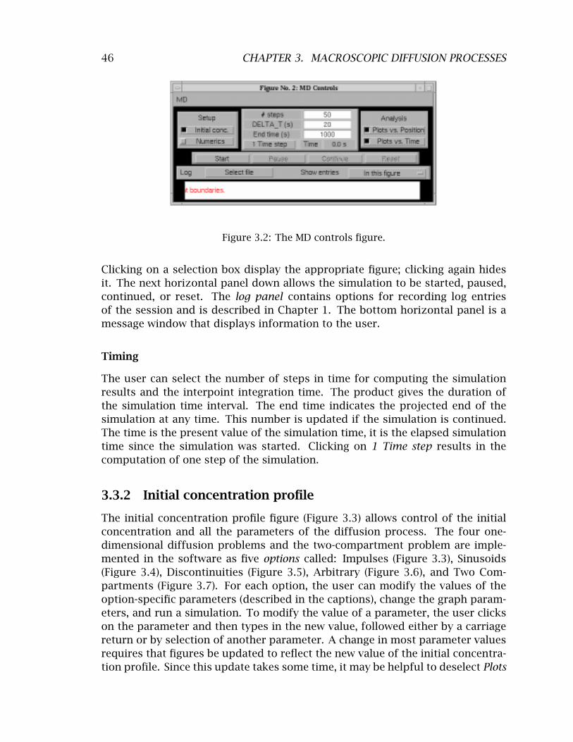
46 CHAPTER 3. MACROSCOPIC DIFFUSION PROCESSES
Figure 3.2: The MD controls figure.
Clicking on a selection box display the appropriate figure; clicking again hides it. The next horizontal panel down allows the simulation to be started, paused, continued, or reset. The log panel contains options for recording log entries of the session and is described in Chapter 1. The bottom horizontal panel is a message window that displays information to the user.
Timing
The user can select the number of steps in time for computing the simulation results and the interpoint integration time. The product gives the duration of the simulation time interval. The end time indicates the projected end of the simulation at any time. This number is updated if the simulation is continued. The time is the present value of the simulation time, it is the elapsed simulation time since the simulation was started. Clicking on 1 Time step results in the computation of one step of the simulation.
3.3.2 Initial concentration profile
The initial concentration profile figure (Figure 3.3) allows control of the initial concentration and all the parameters of the diffusion process. The four one-dimensional diffusion problems and the two-compartment problem are implemented in the software as five options called: Impulses (Figure 3.3), Sinusoids (Figure 3.4), Discontinuities (Figure 3.5), Arbitrary (Figure 3.6), and Two Compartments (Figure 3.7). For each option, the user can modify the values of the option-specific parameters (described in the captions), change the graph parameters, and run a simulation. To modify the value of a parameter, the user clicks on the parameter and then types in the new value, followed either by a carriage return or by selection of another parameter. A change in most parameter values requires that figures be updated to reflect the new value of the initial concentration profile. Since this update takes some time, it may be helpful to deselect Plots

47 3.3. USER’S GUIDE TO THE SOFTWARE
Figure 3.3: Initial concentration figure for impulses. When the software is initiated, Impulses is the default initial concentration profile. In general, the magnitudes and positions of four impulses can be specified. The positions of each impulse can be set only if its magnitude is non-zero. The boundary type (transparent or reflecting) is selectable, and, if the boundaries are reflecting, the positions of the two reflecting boundaries can be set.

48 CHAPTER 3. MACROSCOPIC DIFFUSION PROCESSES
Figure 3.4: Initial concentration figure for sinusoids. The frequencies and amplitudes of the four sinusoids were chosen to correspond to the first four terms in the Fourier series of a square wave. In general, the amplitudes, frequencies, and phases of four sinusoids can be specified. The frequency and phase of a sinusoid can be set only if its amplitude is non-zero. Only transparent boundaries are available for the sinusoids option.

49 3.3. USER’S GUIDE TO THE SOFTWARE
Figure 3.5: Initial concentration figure for discontinuities. Two discontinuities were used to generate an initial concentration profile that is a rectangular pulse. In general, the magnitude and position of four discontinuities can be specified. The position of a discontinuity can be set only if its magnitude is non-zero. The boundary type (transparent or reflecting) is selectable, and, if the boundaries are reflecting, the positions of the two boundaries can be set.

50 CHAPTER 3. MACROSCOPIC DIFFUSION PROCESSES
Figure 3.6: Initial concentration figure drawn using the arbitrary option. Only the reflecting boundary condition is available for this option, and the positions of the two boundaries is specifiable. The initial profile is drawn on the monitor screen by moving the mouse cursor. The details are described in Section 3.3.5.

51 3.3. USER’S GUIDE TO THE SOFTWARE
Figure 3.7: Initial concentration figure for the two compartments option. In general, specification can be made for the width and the initial concentration in each bath, the membrane width, and the initial membrane concentration profile, drawn with a mouse cursor (as described in Section 3.3.5). The user can also chose how the two baths and the membrane are to be displayed. Selecting the View membrane option displays the membrane and a bit of each bath on each side. Selecting the View baths option displays the membrane and both baths to scale.

52 CHAPTER 3. MACROSCOPIC DIFFUSION PROCESSES
Figure 3.8: The diffusion parameters figure.
vs. position and Plots vs. time from the MD controls figure. All the parameters for each option can be saved in a file and read from a file.
Diffusion parameters
Clicking on Diffusion parameters in the Initial concentration profile figure displays the Diffusion parameters figure (Figure 3.8). This figure allows the user to specify the diffusion parameters (diffusion coefficient, drift velocity, and chemical reaction rate) for each option independently. For the two compartments option these diffusion parameters apply to the membrane and not to the baths.
Graph of initial concentration
The initial concentration is plotted in the Initial concentration profile figure (Figures 3.3-3.7). A check box in the upper right-hand corner allows display of the initial flux. An axis scale can be changed by clicking on its label to display the axis-scale figure which is described in Chapter 1. The new axis limits can be typed into the edit boxes to change the axis. In addition, there are two markers that are indicated by two triangles on the abscissa. These markers indicated positions at which the concentration and flux can be displayed as a function of time. The positions of these markers can be controlled numerically or graphically. Numerical control is achieved by typing into the appropriate text edit box. Graphical control is achieved by clicking on the abscissa axis. The left marker is controlled by clicking the left button on a two-button mouse or by clicking the button on a single-button mouse. The right marker is controlled by clicking the right button on a two-button (or three-button) mouse or by shift-clicking the button on a single-button mouse.
3.3.3 Numerics
Clicking on Numerics in the MD Controls figure displays the Numerics figure (Figure 3.9). The numerics figure controls the spatial resolution of the simulation. The upper portion of this figure deals with those computations that make use of exact solutions of the diffusion equation (i.e., all one-dimensional diffusion problems with transparent boundaries). For this case, the user can select the

53 3.3. USER’S GUIDE TO THE SOFTWARE
Figure 3.9: The numerics figure.
number of spatial points at which the solution is computed. The larger the number of points, the higher the spatial resolution of the computation and the longer it will take to complete the computation. The lower portion of this figure deals with those computations that use numerical integration of the diffusion equation (i.e., all one-dimensional diffusion problems with reflecting boundaries and the two-component diffusion problem). The user can choose to select the number of points in space at which the solution is computed. The user has a choice in how the interpoint integration time is to be determined. The numerical method is stable provided an inequality that relates the temporal and spatial resolution is satisfied. If Auto-link with DELTA_T is selected, the simulation determines the integration time to satisfy the inequality and to guarantee a stable integration method which results in an accurate solution. If this choice is not selected, the user can choose the temporal resolution (integration time) and spatial resolution independently. However, with this choice there is no guarantee that the solution will be accurate.
3.3.4 Analysis figures
There are two figures that display the solute concentration and flux during a simulation. The Plots versus position figure displays the concentration and/or the flux as a function of position at each instant in time during the simulation (Figure 3.10). The current simulation time is displayed near the top of the figure. Axes limits can be changed by clicking on the axes labels to display the axis-scale figure. The two green triangular markers mirror the markers shown in the Initial concentration profile figure. With the Two compartments option, the user can also chose how the two baths and the membrane are to be displayed. Selecting the View membrane option displays the membrane and a bit of each bath on each side. Selecting the View baths option displays the membrane and both baths to scale.
The Plots versus time figure (Figure 3.11) displays the concentration and/or the flux as a function of time during the simulation for two positions selected by the markers found in both the Initial concentration profile figure and the Plots versus position figure (Figure 3.10). The locations of the markers are indicated at

54 CHAPTER 3. MACROSCOPIC DIFFUSION PROCESSES
Figure 3.10: Plots versus position figure.
Figure 3.11: Plots versus time figure.

55 3.3. USER’S GUIDE TO THE SOFTWARE
the top of the figure. Axes limits can be changed by clicking on the axes labels to display the axis-scale figure.
3.3.5 Arbitrary concentration profiles
For the Arbitrary and Two compartments options, the user can draw an arbitrary initial concentration profile by clicking on the Draw initial profile button and can erase an existing profile by selecting the Erase initial profile button. Clicking on the Draw initial profile button will erase the existing profile.
Drawing a profile consists of generating a list of concentration values at a corresponding array of positions. The user selects these points by moving the mouse and clicking any mouse button. As the pointer moves within the plotting field in the Initial concentration profile figure, a line joins the last point which was selected to the current pointer position. There are two modes of action that the user can use to draw the profile:
Clicking a mouse button within the axes of the graph adds a position and • concentration value to the coordinate lists and draws a line segment from the previous point to the current point. In this manner, the user can construct a profile made up of line segments.
Moving the mouse while a mouse button is held down causes a series of • points to be added to the coordinate lists. In this manner, the user can construct more complicated curves.
The two methods can be combined in drawing a single profile. As soon as a complete profile has been drawn, the drawing routine terminates and stores the profile data.
There are some additional rules of operation for drawing initial profiles. When a button is pressed, the position and concentration that are added to the coordinate arrays depend on the pointer location:
A button press at a position that does not lie to the right of the previous • point is ignored, in order to ensure that the user-drawn concentration profile is a single-valued function of position.
If a button is pressed within the graph axes, then the coordinates of the • pointer location are added to the list.
If a button is pressed outside the boundaries of the graph (but still within • the graph window), then the point that is added to the list is the point of intersection between the graph boundary and a line from the previous point to the current position. Thus, while a profile is being drawn, it is constrained to lie entirely within the boundaries of the graph.
56 CHAPTER 3. MACROSCOPIC DIFFUSION PROCESSES
By default in the arbitrary option, the concentration at the left-hand point of • the profile is zero. The user can change the first value, however, by making the first button press at the desired vertical location but to the left of the concentration axis. In the two components option, the concentration at the left-hand point of the profile is set equal to the concentration in the left bath (bath #1), and the concentration at the right-hand point of the profile is set equal to the concentration in the right bath (bath #2).
Clicking outside the Initial concentration profile figure at any time aborts the drawing procedure.
3.4 Problems
Problem 3.1 In this problem you will investigate the space-time evolution of solute diffusion from a point source. For all parts of this problem use a single impulse and transparent boundaries. Set the impulse strength to 100 moles/cm2, place the impulse at position 0.5 cm, and set the drift velocity and the reaction rate to zero. Set the marker positions to 0.55 and 0.6 cm unless indicated otherwise. Set the diffusion coefficient to 10−5 cm2/s and run the simulation for 1000 seconds. Obtain a plot of the concentration and flux on appropriate ordinate scales. You should obtain the spatial distribution of the concentration and the flux at 1000 seconds and both variables as a function of time at the two marker positions. Repeat these two steps for a diffusion coefficient of 4 × 10⁻⁵ cm2/s.
a. Describe qualitatively the effect of the change in diffusion coefficient on the spatial distribution of concentration. Be brief.
b. For both values of the diffusion coefficient, determine the maximum amplitude of the concentration versus position and the width of the spatial distribution of concentration at an amplitude that is e−1 of its peak value. Explain the numerical values of all four measurements. Be brief and precise; state your assumptions explicitly.
c. For the diffusion coefficient at 10−5 cm2/s, examine the concentration versus time at the two positions 0.55 and 0.6 cm. Describe qualitatively the differences in concentration versus time at the two positions. Be brief.
d. For the diffusion coefficient at 10−5 cm2/s, measure the maximum concentration as a function of time at the two positions and the time of occurrence of this maximum. Explain the values of all four measurements. Be brief and precise; state your assumptions explicitly.
e. Explain the shape of the spatial distribution of flux for a diffusion coefficient of 10−5 cm2/s.

57 3.4. PROBLEMS
f. Explain the relation between the flux and concentration versus time at location 0.55 cm for a diffusion coefficient of 10−5 cm2/s.
g. Rerun the simulation for a diffusion coefficient of 10−5 cm2/s at positions 0.45 and 0.55 cm. Explain the differences in the flux as a function of time for these two locations.
Problem 3.2 This problem deals with the solution from a point source in the presence of drift. Set the impulse strength to 100 moles/cm2; place the impulse at position 0.5 cm; set the diffusion coefficient to 10−5 cm2/s, and the reaction rate to zero. Set the marker positions to 0.75 and 0.9 cm unless indicated otherwise. The parts of this problem that deal with reflecting boundaries are solved numerically. To decrease the time taken for these computations, consider decreasing the spatial resolution of the computation to 10 points.
a. Set the boundary conditions to transparent and the drift velocity to zero and run the simulation for 1000 s. Now set the drift velocity to 10−4 cm/s and run the simulation again for 1000 s. Describe the effect of the drift on the spatial distribution of concentration. Account quantitatively for the position of the peak of the spatial distribution at 1000 s.
b. Set the boundary conditions to reflecting and the drift velocity to zero. Run the simulation until the spatial distribution is no longer a function of time. This is the equilibrium distribution. What is the spatial distribution at equilibrium? Explain your answer.
c. Set the boundary conditions to reflecting, the drift velocity to 10−4 cm/s, and run the simulation. Describe the effect of drift on the spatial distribution of concentration. Illustrate your description with printed copies of the distribution at characteristic times.
d. With the boundary conditions still set to reflecting and the drift velocity 10−4 cm/s, determine the equilibrium spatial distribution of concentration. Account quantitatively for this distribution.
e. It is known that the density of air decreases exponentially with distance above the earth’s surface. Explain this phenomenon.
Problem 3.3 As shown elsewhere (Weiss, 1996a, Chapter 3), two-compartment diffusion is based on 4 assumptions:
1. The two compartments are well-mixed so that the concentrations of solute n are uniform and have values at time t of c1
n(t).n(t) and c2
2. Solute particles are conserved, e.g., there is no chemical reaction present that either creates or destroys particles.

58 CHAPTER 3. MACROSCOPIC DIFFUSION PROCESSES
3. The membrane is sufficiently thin and the number of solute particles contained in the membrane at any time is negligibly small.
4. The membrane is sufficiently thin that at each instant in time the concentration profile in the membrane is in steady state.
This problem concerns the conditions for the validity of assumptions 3 and 4. Specifically, you will explore the effect of bath dimensions on two-compartment diffusion without making these two assumptions.
In all parts of the problem, use the Two compartments option of the software. Set the membrane width to 0.01 cm, and the concentration of bath #1 to 70 and bath #2 to 10 mol/cm3. Leave the drift velocity and reaction rate at 0 and the diffusion coefficient at 10−5 cm2/s. Set the parameters of the plot of concentration versus position so that the membrane and a little of each bath are visible on the screen — select membrane view. Note that the left edge of the membrane is at a position of 0 cm. Draw some initial concentration in the membrane. Make sure all ordinate scales on all plots are 0 to 100 mol/cm3. Keep these parameters fixed throughout this problem. To reduce the time taken for the computation reduce the spatial resolution in the membrane to 10 points in space. The software will determine the time increment (DELTA_T). Initially set the number of steps so that the end time is 5 s.
For each of the pairs of bath widths — Bath #1 = 1 cm, Bath #2 = 1 cm; Bath #1 = 0.1 cm, Bath #2 = 0.1 cm; Bath #1 = 0.01 cm, Bath #2 = 0.01 cm; Bath #1 = 0.01 cm, Bath #2 = 0.05 cm; Bath #1 = 0.001 cm, Bath #2 = 0.001 cm; — answer the following questions.
a. Assess the validity of assumption 4.
i. Make rough estimates of both the steady-state (�ss ) and equilibrium (�eq ) time constants from the computations.
ii. Estimate the same two time constants based on theoretical considerations (Weiss, 1996a, Chapter 3).
iii. What is your conclusion based on your computations and your estimates of time constants?
b. Assess the validity of assumption 3.
i. Before you do the computation, make an estimate of the final concentration in each bath. Then do the computation, and check your initial estimates against the computed values
ii. If they differ, explain the basis of the difference.
iii. How good is the assumption that the quantity of solute in the membrane is negligible? If you decide that the quantity of solute in the membrane is not negligible, design a simulation experiment to test your conclusion.

59 3.4. PROBLEMS
e. Are the bath concentrations exponential functions of time? Explain.
Problem 3.4 Some problems in diffusion with a reflecting boundary can be solved by using the solution for a transparent boundary and the method of images to match the reflecting boundary condition. This problem explores the successes and pitfalls of this method. In all parts of this problem, set the drift velocity to zero, the reaction rate to zero, and the diffusion coefficient to 10−5 cm2/s unless state otherwise. The parts of this problem that deal with reflecting boundaries are solved numerically. To decrease the time taken for these computations, consider decreasing the spatial resolution of the computation to 10 points.
a. Use reflecting boundaries, and an initial impulse of concentration of strength 100 moles/cm2 located at 0.2 cm. Run the simulation for 1000 s and obtain a print of the spatial distribution of concentration at time 1000 s and the concentration versus time at locations 0 and 0.3 cm.
b. At a reflecting boundary, the flux must be zero. Change the boundary condition to transparent and determine the parameters of two impulses: one to match the left boundary condition and another to independently match the right boundary condition. Run the simulation again and compare with the results in part a. Does this “method of images” work exactly? Explain.
Problem 3.5 Diffusion from an initial sinusoidal concentration distribution gives important insights into the space-time evolution of diffusion processes. In all parts of this problem, use a drift velocity of zero, a reaction rate of zero, and a diffusion coefficient of 10−5 cm2/s unless state otherwise.
a. Use an initial concentration that is sinusoidal with amplitude 50 moles/cm2
and a spatial frequency of 1 cycle/cm. Run the simulation for 1000 s and print the spatial distribution of concentration at 1000 s and the concentration versus time at 0.25 and 0.75 cm. Repeat this procedure for sinusoids with the same amplitudes but the following spatial frequencies: 3, 5, and 7 cycles/cm. Summarize your results both qualitatively (in words) and then quantitatively (with suitable calculations).
b. Construct a periodic waveform from four sinusoids with the following amplitudes (moles/cm2) and spatial frequencies (cycles/cm): 105, 1; 35, 3; 21, 5; 15, 7. Run the simulation and observe the spatial distribution of concentration. Summarize your results and relate them to results of part a.
c. Switch to the arbitrary initial distribution option and set the boundary conditions to reflecting. Using the mouse draw an arbitrary, preferably jagged, initial profile. This part of this problem uses a numerical solution method that is time consuming. To decrease the time taken for these computations, consider decreasing the spatial resolution of the computation to 10

60 CHAPTER 3. MACROSCOPIC DIFFUSION PROCESSES
points. Run the simulation and watch the spatial distribution of concentration change. Summarize your results. What is the effect of diffusion on the spatial distribution?

Chapter 4
CARRIER-MEDIATED TRANSPORT
61

62 CHAPTER 4. CARRIER-MEDIATED TRANSPORT
4.1 Introduction
Transport of many solutes including important metabolites (e.g. monosaccharides, amino acids, mononucleotides, phosphates, uric acid, etc.) through cellular membranes is accomplished by membrane-bound carrier molecules that combine with the solute molecule on one face of the membrane, then translocate in the membrane and uncombine at the other face. Thus, transport involves chemical reactions in which the solute binds and unbinds with a carrier. This type of transport is called carrier-mediated transport. Carrier-mediated transport has distinctive properties. For example, the relation of flux to concentration saturates, i.e., it does not obey Fick’s law for membranes. In addition, different molecules compete for the carrier. For example, glucose and sorbose (two monosaccharides) compete for the sugar carrier. Hence, transport of one sugar can inhibit transport of another simply by occupying a site to which both can bind.
There are canonical models of carrier-mediated transport that capture important properties of the transport of metabolites through cellular membranes. It is important to understand these canonical models in order to understand how metabolites are transported across these membranes. Derivations of predictions of these models are not particularly difficult to follow; the individual steps are simple. However, the models typically result in messy algebraic expressions that relate flux to concentration and transport parameters. Thus, it is easy to get lost in algebraic manipulation as well as in a sea of parameters so that an intuitive grasp of the models becomes illusive. The intent of this software is to allow the user to develop intuition for these models.
4.2 Description Of The Models
Descriptions of carrier-mediated transport as well as models of such transport processes can be found elsewhere (Stein, 1986; Weiss, 1996a). Here we consider three models and list both the assumptions and the important results. First, we consider the steady-state behavior of a simple, four-state carrier that binds one solute Then, we consider the steady-state behavior of a simple, six-state carrier that binds two solutes with different affinities. Finally, we consider both the transient and the steady-state behavior of a general, four-state carrier model that binds one solute.

63
c
4.2. MODELS
Membrane
�EinE no E
Ki S Ko S
τES αES
τE
Ei Eo
ESi ESo
Si + So +
Extr
acel
lula
r
Figure 4.1: Kinetic diagram ofthe simple, four-state carrier that binds one solute.
Intr
acel
lula
r
i S
o Sc
αEi onES �S �ES nES =
4.2.1 Steady-state behavior of a simple, four-state carrier that binds one solute
Assume that the membrane contains NET moles of carrier per unit area of mem-brane.1 Each of these carriers exist in one of four states labeled ESi , ESo , Ei, and Eo (Figure 4.1). In the ES states, the solute S is bound to the carrier E; in the E state the carrier is unbound. In the ESi and Ei states, the carrier, bound and unbound, communicates with the solution on the inner side of the membrane. In the ESo and Eo states, the carrier, bound and unbound, communicates with the solution on the outer side of the membrane. The densities of carrier in the
i o ofour states are nES , nES , nEi , and nE moles per unit area of membrane. The fluxes
of bound and unbound carrier are �ES and �E and the flux of solute is �S . The flux is defined as positive when the flux is in the outward direction; the units are in moles per unit area per second. The model is defined by the following assumptions:
The total amount of carrier, bound and unbound, is constant, i.e. the sum • of the carrier density over all of its states equals the total density of carrier in the membrane
NET i o i o (4.1)= nES + nES + nE + nE.
Since the carrier resides permanently in the membrane, the total flux of • carrier must be zero, i.e.
�ES + �E = 0. (4.2)
The only time the solute crosses the membrane is when it is bound to the • carrier; ESo is assumed to undergo a reversible change in conformation to the form ESi. The unbound carrier is assumed to undergo a similar reaction
1Because the kinetic equations for binding of the carrier to the solute are analogous to those of the binding of an enzyme to its substrate, the carrier is denote by E which stands for enzyme.

� �� � � �
64 CHAPTER 4. CARRIER-MEDIATED TRANSPORT
between the two conformations Ei and Eo. These two reactions are assumed to be first-order reactions with forward and reverse rate constants, τE , τES , αE , and αES , so that the fluxes are defined as follows:
ES, (4.3)�ES = �S τESnESi − αESno =
τEnEi − αEno�E E. (4.4)=
In the simple model, the binding reactions at the membrane interfaces are • assumed to be so rapid, compared to the rate of transport of solute across the membrane, that the membrane interface reactions are assumed to be at equilibrium, i.e.,
co o i i
S and cSnE KiSnE Ko
S, (4.5)no ES
= nESi =
where Ko and Ki S S are the dissociation constants on the two membrane interfaces.
These equations can be solved to determine the n’s in terms of the concentrations and transport parameters. Equations 4.3 and 4.4 can be used to determine the �’s. Combining Equations 4.2, 4.3, and 4.4 yields
(τESnESi − αESno
ES) + (τEnEi − αEno 0. (4.6)E) =
Equations 4.1, 4.5, and 4.6 can be expressed as a matrix equation as follows:
iKi 0S i0 0−c
0 nS ES���⎤
���⎤
⎪⎪⎪⎣
⎪⎪⎪⎣=���⎤
⎪⎪⎪⎣Ko S −co
S
−αE
no ES
ni E
0 0 0
. (4.7)τES −αES τE
1 1 no E NET1 1
The first two rows correspond to the two relations in Equation 4.5. The third row results from Equation 4.6, and the fourth row corresponds to Equation 4.1. This set of simultaneous equations has the following solutions (Weiss, 1996a):
icS(αEKo
S )i D1
, (4.8)nES = NET S + αESco
i S (τEK
i no ES = NET
coS + τEScS), (4.9)D1
S(αEKoKi S + αESco
inE = NET D1
S ), (4.10)
i S (τEK
iKo S + τEScS)no
E = NET D1 , (4.11)
where
i iD1 = (αEKo S )(K
iS + τEScS)(K
o S ). (4.12)S + αESco
S + cS) + (τEKi S + co

65
c
c
4.2. MODELS
Membrane i �S �ES o
ni E no E
nES nES
Ki S Ko S
τES αES
τE αE
�E
=
Ei Eo
ESi ESo
Ki R Ko R
τERERi ERo
i ocS S
Extr
acel
lula
r
Figure 4.2: Kinetic diagram of a simple,six-state carrier that binds two solutes (Sand R).
Intr
acel
lula
r
Si So + +Ri Ro
i ocR R
i αER onER nER �R = �ER
�S and �E can be obtained from Equations 4.3 and 4.4. The flux of solute can also be expressed in terms of the uni-directional fluxes
as �S =
≤�S −
��S ,
where ≤�S = τES ni ES and
��S = αES no
ES .
4.2.2 Steady-state behavior of a simple, six-state carrier that binds two solutes
The simple, four-state carrier shown in Figure 4.1 can be extended to account for the binding of two solutes that compete competitively for binding sites on the carrier (Figure 4.2). In this scheme, solutes S and R combine with carrier E but with different affinities. The binding to solute S has dissociation constants Ki S
and Ko R and Ko
S and the binding to R has dissociation constants Ki R. The kinetic equations are analogous to those derived for the simple, four-state
carrier except that the carrier now has 6 states:
The total amount of carrier, bound and unbound, is constant, i.e. the sum• of the carrier density over all of its six states equals the total density of carrier in the membrane
NET nESi + no i
ES + nER + no iE, (4.13)ER + nE + no =

� �� � � �
66 CHAPTER 4. CARRIER-MEDIATED TRANSPORT
where NET is the total density of carrier in the membrane.
Since the carrier remains in the membrane, the net flux of carrier must be • zero
�ES + �ER + �E = 0. (4.14)
The fluxes are related to the carrier densities so that •
(τESnESi − αESno�ES = �S ES). (4.15)=
(τERnERi − αERno�ER = �R ER). (4.16)=
o�E (τEnEi − αEnE). (4.17)=
In the simple model, the reactions at the membrane interfaces are assumed • to take place so rapidly, compared to the rate of transport of solute across the membrane, that the membrane interface reactions are assumed to be at equilibrium, i.e.,
Sno i i co i
E Kico
E KocSnE Ki Rn
o
Ko cRni
no S , i S and no
E R, R, (4.18)
ES
= nES
= ER =
nERi =
where Ko S , K
o R are the dissociation constants for solutes S and R,S , K
i R and Ki
respectively at the two membrane interfaces.
Combining Equations 4.14 and 4.15, 4.16, and 4.17 yields
ES) + (τERnERi − αERno(τESnES
i − αESno ER) + (τEnE
i − αEno 0. (4.19)E) =
It is of interest to obtain the flux of solutes S and R as a function of both concentrations and the transport parameters Ki S , K
i R, τES , τER, τE , αES , αER,S , K
o R, Ko
αE , and NET . Therefore, it is useful to regard the system of algebraic equations given by Equations 4.14 through 4.19 as a set of 6 equations in the 6 unknowns i
ES , nER, no inES , no i
ER, nE , and no E . These can be written in matrix form as follows:
iKi 0 0 0S i0 0−c
0 nS ES �������⎤
�������⎤
⎪⎪⎪⎪⎪⎪⎪⎣
⎪⎪⎪⎪⎪⎪⎪⎣
=
�������⎤
⎪⎪⎪⎪⎪⎪⎪⎣
Ko S −co
S
0 no ES0 0 0 0
0 0 0
iKi 0R i ER0 0 −c
0 nR . (4.20)Ko
R −co R
−αE
no ER0 0 0 i EτES −αES τER −αER τE
1 1 1 1 nno E NET1 1
The first four rows correspond to the four relations in Equation 4.18. The fifth row results from Equation 4.19, and the sixth row corresponds to Equation 4.13. This set of simultaneous equations has solutions (Weiss, 1996a):
i nES NET
R(αEKo
R + αESco R + αERKo
R)i cSKi
SKo
SKo
Sco
, (4.21)= D2

67 4.2. MODELS
i i
ES NET co
R(τEKi
R + τEScSKi
ScR)SKo
SKi
R + τERKi no , (4.22)= D2
Ki i SK
o SK
o Sc
o
nER = NET ScR(αEK
o R + αESco
R + αERKo R)i , (4.23)
D2
i i
ER = NET co
S (τEKi
R + τEScSKi
ScR)RKo
SKi
R + τERKi no , (4.24)D2
SKi
SKo
SKo
Sco
nE = NET Ki R(αEK
o R + αESco
R + αERKo R)i , (4.25)
D2
i i
E = NET Ko
R(τEKi
R + τEScSKi
ScR)SKo
SKi
R + τERKi no , (4.26)D2
where
D2 S(ci
RτE)(Ko
R + co R + Ko
R) +Ki RτER + Ki SKo
SKo
Sco =
i i S (c
o RαE)(K
i R + cSK
i ScR) +
i Ko
RαER + Ko SKi
R + Ki
cSKi
SKo
SKo
Sco
RτES(Ko
R + co R + Ko
R) +i i
SKo
SKi
R + Kico RαES(K
i R + cSK
i ScR). (4.27)
The fluxes can be computed using Equations 4.15-4.17. The solute fluxes can also be expressed in terms of the uni-directional fluxes
as
�S
≤�S −
��S,=
�R
≤�R −
��R,=
where
≤�S τESnES
i and ��S = αESno
ES,=
o≤�R τERnER
i and ��R= αERnER.=
4.2.3 Transient and steady-state behavior of a general, four-state carrier that binds one solute
Transient solution
Suppose that in the simple, four-state carrier model shown in Figure 4.1, the assumption that the interfacial binding reactions are fast is dropped. The model which results is called the general, four-state carrier model and the kinetic diagram for this model is shown in Figure 4.3.
This model is defined by the following assumptions:
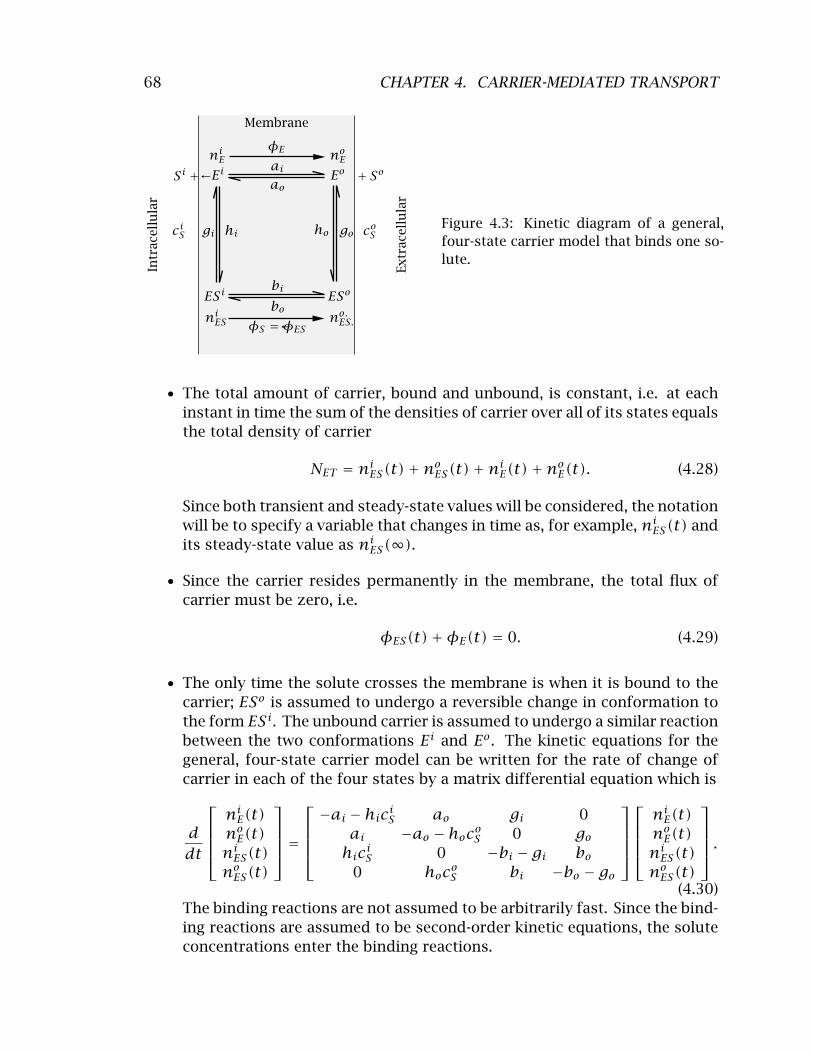
� � � �� �
c
68 CHAPTER 4. CARRIER-MEDIATED TRANSPORT
Membrane
i �E onE nE + Ei Eo
ESi ESo
ai ao
bi
gi gohi ho
Si + So
Extr
acel
lula
r
Figure 4.3: Kinetic diagram of a general,four-state carrier model that binds one solute.
Intr
acel
lula
r
i S
o Sc
boi onESnES �S �ES=
The total amount of carrier, bound and unbound, is constant, i.e. at each • instant in time the sum of the densities of carrier over all of its states equals the total density of carrier
ES(t) + nEi (t) + noNET nES
i (t) + no E(t). (4.28)=
Since both transient and steady-state values will be considered, the notation will be to specify a variable that changes in time as, for example, nES
i (t) and its steady-state value as nES
i (�).
Since the carrier resides permanently in the membrane, the total flux of • carrier must be zero, i.e.
�ES(t) + �E(t) = 0. (4.29)
The only time the solute crosses the membrane is when it is bound to the • carrier; ESo is assumed to undergo a reversible change in conformation to the form ESi. The unbound carrier is assumed to undergo a similar reaction between the two conformations Ei and Eo . The kinetic equations for the general, four-state carrier model can be written for the rate of change of carrier in each of the four states by a matrix differential equation which is
i E(t)
i S
i E(t) −ai − hic
ai 0n ao gi n���⎤
⎪⎪⎪⎣=���⎤
���⎤
⎪⎪⎪⎣
⎪⎪⎪⎣d
dtno E(t) −ao − hoco
S
0 no E(t) 0 go .i
ES(t) i S
i ES(t) hic −bi − gi bo
bi n nno ES(t) 0 hoco
S no ES(t) −bo − go
(4.30) The binding reactions are not assumed to be arbitrarily fast. Since the binding reactions are assumed to be second-order kinetic equations, the solute concentrations enter the binding reactions.

� � � �� � � �
� �� � � �
4.2. MODELS 69
The four kinetic equations are not independent; e.g., the fourth can be derived from the first three equations. Thus, the fourth equation can be eliminated and no ES(t) can be eliminated using the conservation of carrier relation,
ES(t) = NET − nEi (t) − nono
E(t) − nESi (t), (4.31)
to yield the matrix equation
0i E(t)
i S
i E(t) −ai − hicn ao gi nd �⎤
⎪⎣�⎤
�⎤⎪⎣
⎪⎣�⎤gono
E(t) S−ao − go − hoco no E(t) NET .ai − go
i ES(t)
i −go +
dt=
i ES(t) S − bo −bo −bi − gi − bo
(4.32) This matrix equation can be solved for the three carrier densities and Equation 4.31 can be used to solve for the fourth density. The solution for each of the carrier densities has the form
nj(t) = Aj1eφ1t + Aj2eφ2t + Aj3eφ3t, (4.33)
where the nj ’s are the four carrier densities, the φ’s are the three non-zero eigenvalues of the system, and the A’s are the residues. This solution is valid when the eigenvalues are distinct. All 4 carrier densities have the same 3 eigenvalues, but in general, the residues differ. Since the rate constants and concentrations are all positive quantities, it can be shown that all the eigenvalues have negative real parts. Both the eigenvalues and residues are functions of the rate constants and the solute concentrations. Hence, the solutions yield the carrier densities
ES(t), nEi (t), and no(nES
i (t), no E(t)) as functions of time for any values of the con
centrations of solute S and of the transport parameters ai, ao, bi, bo, gi, go, hi, ho, and NET .
Steady-state solution
In the steady state, the density of carrier in each of its four states is constant and the derivative terms on the left-hand side of Equation 4.30 are zero. As noted previously, the four equations are not independent. Thus, one of the equations can be eliminated. However, conservation of carrier leads to an independent constraint which can be added to the three independent steady-state equations to yield the following four steady-state equations
hic bon n
i S)
i−(ai + hicai
E(�) no E(�)
0 0ao gi n���⎤
���⎤
⎪⎪⎪⎣
⎪⎪⎪⎣
���⎤
⎪⎪⎪⎣−(ao + hoco
S ) 0
0 0go . (4.34)i S
ihic −(bi + gi) bo
1 ES(�) no ES(�) NET
0=n
1 1 1
The solutions (Weiss, 1996a) are ratios of sums of products of rate constants
i Mo E E(�) Mo nES
i (�) Mi nonE(�) Mi no
DE , ES ES(�) ES
NET = D , NET
= NET
= D , NET
= D, (4.35)
⎪⎣

70 CHAPTER 4. CARRIER-MEDIATED TRANSPORT
where
Mi S ,E aobigo + aogigo + aobogi + bogihoco =
Mo i E aibigo + aigigo + aibogi + bigohicS,=
i iMi aibohoco i S , (4.36)ES S + aogohicS + aobohicS + bohihocSco =
S + aigihoco i iMo aibihoco S + aobihicS + bihihocSc
o ES S ,=
D Mi E + Mi
E + Mo ES + Mo
ES.=
The steady-state flux is found elsewhere and equals (Weiss, 1996a) i
Sno
−�E(�) = �S(�) = �ES(�) = bigohicSnE
i (�) − bogihoco E(�). (4.37)
bigo + bogi + gigo
These equations yield the values of the n(�)’s and the �(�)’s in steady state as a function of the concentrations of solute S and of the transport parameters ai, ao, bi, bo, gi, go, hi, ho, and NET .
The flux of solute can also be expressed in terms of the uni-directional fluxes as ≤
�S(�) = �S (�)−��S (�),
where
bigohicSnEi (�)i≤
�S (�) = bigo + bogi + gigo
, o obogihocSnE(�) .
��S (�) =
bigo + bogi + gigo
4.3 Numerical Methods And Parameters
4.3.1 Numerical methods
The steady-state values of the carrier densities and the carrier fluxes are algebraic functions of the solute concentrations and of the parameters. They could have been computed directly from the steady-state matrix equations for each carrier model. However, it proved to be faster to compute these quantities directly from the solutions of these matrix equations which are: Equations 4.3-4.4 and Equations 4.8-4.11 for the simple, four-state carrier, Equations 4.15-4.17 and Equations 4.21-4.26 for the simple, six-state carrier, and Equations 4.35-4.37 for the general, four-state carrier.
The transient solution for the general, four-state carrier was obtained by solving Equation 4.32 numerically using MATLAB’s ode15s routine for solving sets of ordinary differential equations. The solution for 3 of the 4 carrier densities were computed; the fourth was computed from Equation 4.31. Eigenvalues of the matrix of rate constants (Equation 4.32) were computed to aid the user in choosing a time scale for displaying transient responses. Eigenvalues were computed using MATLAB’s eig function.

4.4. USER’S GUIDE 71
4.3.2 Choice of numerical parameters
Simple models
The software enables the user to compute the n’s and �’s for any values of the parameters, the τ’s, α’s, K’s, NET , and the concentrations of solute, the c’s. The software is initiated with default parameters chosen to approximate hexose transport in human erythrocytes (Carruthers, 1984; Stein, 1986) assuming a symmetric transport scheme. The density of carriers was set to NET 10 pmoles/cm2.= The dissociation constant of solute S was set to approximate that of D-glucose, Ki Ko 2 µmoles/cm2, and that of R was set to that of a solute to which S S= = the carrier binds with lower affinity, approximating that of D-xylose, so that Ki Ko 200 µmoles/cm2. All the rate constants were set equal with a value R R= = that made the maximum flux 100 pmoles/cm2-s so that τES αES τER= = = αER = τE = αE = 20 s−1. The concentrations of solute were chosen arbitrarily as
ifollows: cS 2, c0 1, ci R = 2, co 1 µmoles/cm3.S= = R =
General model
[To be written]
4.4 User’s Guide
When the program is selected, 3 figures are displayed (in addition to MATLAB’s command window): Controls, Parameters, and State. The controls figure controls the software. The remaining figures are for steady-state interactive analysis of the simple, four-state carrier. In the interactive mode, any parameter of the carrier model can be changed and the resulting steady-state values of carrier densities and fluxes are displayed immediately. The same steady-state interactive analysis is available in all three models: the simple symmetric, four-state carrier; the simple symmetric, six-state carrier; and the general, four-state carrier. Additional modes of analysis allow plotting the steady-state values of carrier densities and fluxes as continuous functions of a user-specified model parameter. In addition, for the general, four-state carrier, the user can observe transient changes in carrier densities in response to a change in parameters. All of these modes of analysis are selected using the controls figure.
4.4.1 CMT controls
The part of the controls figure (Figure 4.4) below the menubar is divided into five panels. The model panel allows the user to choose a particular model for analysis. The analysis panel allows the user to choose among the various modes of analysis available in the software by clicking on the appropriate button. The

72 CHAPTER 4. CARRIER-MEDIATED TRANSPORT
Figure 4.4: Controls figure.
Figure 4.5: Units of all variables in the carrier models.
miscellaneous panel allows the user to display the units for all variables used by the software (Figure 4.5). The log panel contains options for recording log entries of the session and is described in Chapter 1. The message panel at the bottom of the controls figure is used to send messages to the user.
4.4.2 Model
Clicking on model in the controls figure allows selection of three models of carrier-mediated transport. Selecting a different model will initiate the steady-state, interactive analysis for that model. The models are listed below.
Simple, four-state: refers to the simple, four-state carrier that binds one solute. This is the default model that is displayed when the software is initialized. The parameters and state figures associated with this model are shown in Figure 4.6.
Simple, six state: refers to the simple, six-state carrier that binds two solutes shown in Figure 4.7.
General, four-state: refers to the general, four-state carrier that binds one solute shown in Figure 4.8.

73 4.4. USER’S GUIDE
Figure 4.6: Parameters and state figures for the simple, four-state carrier model that binds one solute.

74 CHAPTER 4. CARRIER-MEDIATED TRANSPORT
Figure 4.7: Parameters and state figures for the simple, six-state carrier that binds two solutes.

75 4.4. USER’S GUIDE
Figure 4.8: Parameters and state figures for the general, four-state carrier that binds one solute.
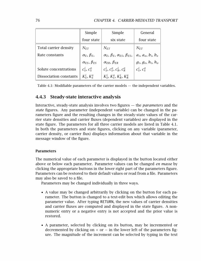
76 CHAPTER 4. CARRIER-MEDIATED TRANSPORT
Simple Simple General
four state six state four state
Total carrier density NET NET NET
Rate constants τE , αE , τE , αE , τES , αES , ai, ao, bi, bo
Solute concentrations
Dissociation constants
τES , αES
ci S , co S
Ki S , Ko S
τER, αER
ci S , co S , c
i R, co
R
Ki S , Ko S , K
i R , K
o R
gi, go, hi, ho
ci S , co S
Table 4.1: Modifiable parameters of the carrier models — the independent variables.
4.4.3 Steady-state interactive analysis
Interactive, steady-state analysis involves two figures — the parameters and the state figures. Any parameter (independent variable) can be changed in the parameters figure and the resulting changes in the steady-state values of the carrier state densities and carrier fluxes (dependent variables) are displayed in the state figure. The parameters for all three carrier models are listed in Table 4.1. In both the parameters and state figures, clicking on any variable (parameter, carrier density, or carrier flux) displays information about that variable in the message window of the figure.
Parameters
The numerical value of each parameter is displayed in the button located either above or below each parameter. Parameter values can be changed en masse by clicking the appropriate buttons in the lower right part of the parameters figure. Parameters can be restored to their default values or read from a file. Parameters may also be saved to a file.
Parameters may be changed individually in three ways.
A value may be changed arbitrarily by clicking on the button for each pa• rameter. The button is changed to a text-edit box which allows editing the parameter value. After typing RETURN, the new values of carrier densities and carrier fluxes are computed and displayed in the state figure. A nonnumeric entry or a negative entry is not accepted and the prior value is restored.
A parameter, selected by clicking on its button, may be incremented or • decremented by clicking on + or − in the lower left of the parameters figure. The magnitude of the increment can be selected by typing in the text

4.4. USER’S GUIDE 77
edit box in the lower left part of the parameters figure. The state figure is updated with each incremental change in the parameter.
A parameter, selected by clicking on its button, may be incremented or • decremented repeatedly by clicking on the repeat button to the right of the + or to the left of the −, respectively. The state figure is updated with each incremental change in the parameter. Clicking on the repeat button again stops the repetitive process.
In the general, four-state carrier, passive transport of solute (also called the principle of detailed balance) requires that (Weiss, 1996a)
aihobogi = aohibigo.
When this condition is violated, a warning messages is displayed in the message window of the parameters figure, and the ratio
aohibigo r = aihobogi
is displayed.
State
The steady-state values of carrier densities and carrier fluxes are displayed below each quantity for the particular set of parameters shown in the parameters figure. These quantities are also displayed graphically. Carrier densities are displayed with bar graphs that represent the relative densities of carrier in each states. Both
i E , nES , and nofour-state carriers display nE
i , no ES . The six-state carrier displays nE
i , no i E , nES , n
o i ES , nER , and no
ER . The carrier fluxes are displayed with thick arrows in the center of the figure. No arrow is displayed when the flux is zero . The direction of the arrow indicates the direction of the flux. The color of the arrow indicates the relative magnitude of the carrier flux; a small magnitude flux has a black arrow, a large magnitude flux has a bright red arrow.
4.4.4 Steady-state graphic analysis
Selection of graphic analysis in the controls figure, displays the steady-state graphic analysis figure (Figure 4.9). This figure allows the user to plot any variable versus any of the parameters of the carrier-mediated transport model. Use of this figure is described in detail in Chapter 1. The variables are listed as: flux E
i �S .for �E , flux ES for �ES , n E i for nE , . . . , efflux S for ≤

78 CHAPTER 4. CARRIER-MEDIATED TRANSPORT
Figure 4.9: The steady-state graphic analysis figure showing a plot of fluxes and carrier densities versus c on linear ordinate and abscissa scales. i
S

79 4.4. USER’S GUIDE
Figure 4.10: The transient analysis figure showing the transient response to the change in parameters shown in Figure 4.11 and using the numerical data shown in Figure 4.12.
4.4.5 Transient analysis
Transient analysis is available only for the generalized, four-state carrier by clicking on transient in the controls figure. This action displays the transient analysis figure (Figure 4.10). Use of the transient analysis figure is described in detail in Chapter 1. Differences occur only in the control of transient analysis panel shown in the upper left panel of the figure. We describe this panel only.
Set up transients. Clicking on this item displays the set up transients figure shown in Figure 4.11. The first column of this figure shows all the 11 independent variables for the general, four-state carrier. The initial values are shown in the second column and the final values are shown in the fourth column. The initial values can be changed individually by typing in the new value in the appropriate text edit box. The third column gives several options for changing any particular variable. Several independent variables can be changed. Clicking on Done terminates selection of variables to be changed.

80 CHAPTER 4. CARRIER-MEDIATED TRANSPORT
Figure 4.11: The set up transients figure.

81 4.5. PROBLEMS
Figure 4.12: The transient numerics figure.
The bottom of the figure gives several additional options for changing variables that are explained by positioning the mouse cursor over the option.
Graph n’s. Clicking on this item displays the carrier densities as a function of time.
Numerics. Clicking on this item displays the transient numerics figure which gives information to the user and allows for control of the time scale of the transient response (Figure 4.12). The transient numerics figure displays the eigenvalues of the transient response at the top. These eigenvalues can be computed for the initial or the final values of all parameters by clicking on the appropriate button in this figure. The final value of the time in the plot is determined by the information in the maximum time for transient response panel.
Absolute scale. Selecting this item displays plots of all carrier densities on the same absolute scale.
Relative scale. Selecting this item displays plots of all carrier densities on individual scales so that all the carrier densities are discernible.
Clear plotting axes. Selecting this item clears the plot field.
4.5 Problems
Problem 4.1 This problem is intended to develop your intuition for the steady-state behavior of the simple, four-state carrier model for a single solute. You will observe the effects of changes in parameters on both the flux and the carrier densities. Use the simple, four-state carrier model and start with all the parameters at their default values.
a. What is the relation of �S and �E ? Explain.

82 CHAPTER 4. CARRIER-MEDIATED TRANSPORT
b. What is the relation of the direction of �S to the sign of cS − coiS ? Explain.
c. How does the state of the carrier depend on solute concentration?
i ii. Do changes in cS change nESi and nE ? If so, how? If not, why not?
ii. Do changes in cS change no E ? If so, how? If not, why not? i
ES and no
S change nESi and nE ? If so, how? If not, why not? iii. Do changes in co i
iv. Do changes in co ES and no
S change no E ? If so, how? If not, why not?
Reset all the parameters to their default values, except set τES 100 s−1.=
d. What is the relation of the direction of �S to the sign of cS − coiS ? Explain.
Reset all the parameters to their default values, except set τE αE 0 s−1.= =
e. What is the relation of �S to cS − coiS ? Explain.
Problem 4.2 This problem is designed to explore the functional relation between flux and solute concentration when expressed in different coordinates. Use the simple, four-state carrier model and start with all the parameters at their default values, except set co 0. In parts a through c your job is to estimate the values S = of (�S)max and Ki from the graphs specified, where (�S)max is the maximum S
flux of S with co 0.S =
ia. Obtain a graph of �S versus cS in linear coordinates.
ib. Obtain a graph of �S versus cS in double logarithmic coordinates.
c. Obtain a graph of 1/�S versus 1/ci S .
d. Determine the values of (�S)max and Ki S from the model parameters.
e. Compare the 4 sets of values you have obtained for (�S)max and Ki S .
Problem 4.3 Use the simple, four-state carrier model and start with all the parameters at their default values, except set co 0. Obtain a graph of all four S
i =
carrier states as a function of cS . Some of the these n’s increase, others decrease, while others remain constant. Summarize and explain the results you found.
Problem 4.4 Use the simple, six-state carrier model and start with all the parameters at their default values. Set the solute concentrations of S and R to zero on both sides of the membrane.
a. Explain the initial carrier states and flux values.

83 4.5. PROBLEMS
ib. Increase cS and observe both the carrier states and the flux. What is the irelation of the flux of S to cS ?
i ic. Now set cS 10 and increase cR. How do the fluxes of S and R depend i
= upon cR?
i id. Set cS 10 and co 5. Now increase cR from an initial value of 0. How S= = ido the fluxes of S and R depend upon cR? Pay particular attention to the
direction of the flux of S.
Problem 4.5 The transient response shown in Figure 4.10 appears to show that the carrier densities change discontinuously at t 0 in response to the change = in parameter shown in Figure 4.11. Reproduce this result.
a. On the basis of the theoretical development given in Section 4.2, can the carrier densities change discontinuously in response to a discontinuous change in any of the parameters? Explain.
b. By experimenting with the transient response, explain the results shown in Figure 4.10. Make your explanation as quantitative as possible.

84 CHAPTER 4. CARRIER-MEDIATED TRANSPORT

Chapter 5
HODGKIN-HUXLEY MODEL
85

86 CHAPTER 5. HODGKIN-HUXLEY MODEL
5.1 Introduction
5.1.1 Background
Electrically excitable cells produce action potentials which are important for transmission of information in neurons, for contraction of muscle cells, and for secretion of chemical substances by neurosecretory cells (Aidley, 1989; Hodgkin, 1964; Katz, 1966; Kandel et al., 1991; Keynes and Aidley, 1991; Nicholls et al., 1992; Weiss, 1996b). The macroscopic mechanisms of production of action potentials can be understood in terms of the nonlinear electrical characteristics of cellular membranes first described by Hodgkin and Huxley for the membrane of the giant axon of the squid (Hodgkin and Huxley, 1952). Since the nonlinear properties of the membranes of electrically excitable cells are controlled by the membrane potential, it is relatively simple to understand these mechanisms when the membrane potential is constant, but vastly more difficult when the membrane potential is not constant such as occurs during an action potential. Of course, it is the properties of electrically-excitable cells under the latter conditions that are the most important for the function of these cells.
5.1.2 Overview of the software
The purpose of this software is to allow users to enhance their comprehension of the Hodgkin-Huxley model by providing a complete simulation of the model under space clamped conditions. Any of the parameters of the Hodgkin-Huxley model can be changed by the user and simulation experiments can be done to examine the consequences of the parameter changes. Extensive graphics utilities allow the user to plot any variable versus any other variable in the model. Since the model is built on a block diagram language (SIMULINK), the user can also make changes in the model structure.
5.2 Description Of The Model
Descriptions of the Hodgkin-Huxley model are available elsewhere (Aidley, 1989; Hodgkin, 1964; Katz, 1966; Plonsey and Barr, 1988; Johnston and Wu, 1995; Weiss, 1996b). A summary of this model is given in this section. The model that is the basis of this software is a one-compartment model that represents a space-clamped axon stimulated by means of two electrodes so that the membrane current density and membrane potential are uniform along the length of the axon.

87 5.2. DESCRIPTION OF THE MODEL
+
−
Jm(t)
Vm(t)
Jm(t) Figure 5.1: Schematic diagram and circuit model
JC
−+ −
+ −
+ −
JK JNa JL
GK(Vm, t) GNa(Vm, t) GL
VK VNa VL
of a space-clamped axon in the voltage-clamp configuration.+
Cm Vm(t)
+
− Jm(t)Vm(t)
+
−
Vm(t)
+ −
+ −
+ −
JK JNa JL
GK(Vm, t) GNa(Vm, t) GL
VK VNa VL
Figure 5.2: Schematic di-JC agram and circuit model
of a space-clamped axon in the current-clamp con-
Jm(t) figuration.Cm
5.2.1 Voltage-clamp and current-clamp configurations
Two simple and mutually exclusive stimulus configurations can be used to investigate the model: the voltage-clamp and current-clamp configurations. In the voltage-clamp configuration (Figure 5.1), the simulated space-clamped axon is driven by a voltage source and the membrane current density is computed. In the current-clamp configuration, the simulated space-clamped axon is driven by a current source and the membrane potential is computed.
5.2.2 The membrane current density components
The total membrane current density, Jm, is the sum of the capacitance current density plus the ionic current density
Jm = JC + Jion, (5.1)

88 CHAPTER 5. HODGKIN-HUXLEY MODEL
where the capacitance current density is
dVm(t) (5.2)JC Cm dt,=
and Vm is the membrane potential. The ionic current density can be expressed in terms of its components
Jion = JNa + JK + JL, (5.3)
where the ionic current densities due to sodium, potassium and leakage are
JNa GNa(Vm, t)(Vm(t) − VNa), (5.4)=
JK GK(Vm, t)(Vm(t) − VK), (5.5)=
JL GL(Vm(t) − VL), (5.6)=
and where the Nernst equilibrium potential for the nth ion is defined in terms of the concentrations as follows ⎦ �
RT co nVn =
znF ln i , (5.7)
cn
where R is the molar gas constant, T is absolute temperature, F is Faraday’s constant, and zn, co and ci are the valence, outside, and inside concentrations n n
of ion n, respectively. For a univalent ion, the Nernst equilibrium potential is expressed as ⎦ � co
nVn = 0.08616 (Tc + 273.16) ln (mV), (5.8)icn
where Tc is the temperature in Centigrade.
5.2.3 The membrane conductances
The sodium and potassium conductances are defined as
¯GNa(Vm, t) GNam3(Vm, t)h(Vm, t), (5.9)= ¯GK(Vm, t) GKn4(Vm, t). (5.10)=
5.2.4 The activation and inactivation factors
The first-order kinetic equations for the activation and inactivation factors are written in terms of the rate constants as follows:
dm τm − m(τm + αm), (5.11)
dt =
dh τh − h(τh + αh), (5.12)
dt =
dn τn − n(τn + αn), (5.13)
dt =
where the τ’s and α’s depend upon Vm.

� � � �
89 5.2. DESCRIPTION OF THE MODEL
5.2.5 The rate constants
The dependence of the rate constants on membrane potential has been generalized from the original Hodgkin-Huxley model to allow control of the potential dependence of individual rate constants and to represent approximately the effects of changes in calcium concentration and temperature.
The rate constants are
τm
αm
=
=
−0.1(35 + Vm + �VCa + Vτm) e−0.1(35+Vm+�VCa+Vτm) − 1
KT Km,
4e−(Vm+�VCa +Vαm +60)/18 KT Km,
(5.14)
(5.15)
τh = 0.07e−0.05(Vm +�VCa+Vτh+60) KT Kh, (5.16)
αh
τn
αn
=
=
=
1 1 + e−0.1(Vm+�VCa+Vαh+30) KT Kh,
−0.01(Vm + �VCa + Vτn + 50) e−0.1(Vm +�VCa+Vτn+50) − 1
KT Kn,
0.125e−0.0125(Vm +�VCa+Vαn +60) KT Kn,
(5.17)
(5.18)
(5.19)
where KT is a temperature factor, that is defined as
3(Tc −6.3)/10KT . (5.20)=
KT multiplies all the rate constants; this effect approximates the effect of temperature on the electrical properties of the membrane of the squid giant axon (Huxley, 1959). The factors Km, Kh and Kn have been added to the original Hodgkin-Huxley model to allow changes to be made in the individual rate constants of m, h, and n. The factor �VCa is used to approximate the dependence of rate constants on calcium concentration and is
co
�VCa = 0.03335 (Tc + 273.16) ln Ca − 12.995 (mV). (5.21)icCa
At the normal calcium concentration, the potential �VCa has the value 0. For calcium concentration ratios that differ from the normal value, �VCa differs from 0 and the dependence of the rate constants on the membrane potential is shifted by a term that is proportional to the calcium equilibrium potential. This approximates the effect of a change in calcium concentration on the parameters of squid giant axon membrane (Frankenhaeuser and Hodgkin, 1957). The potentials Vτm, Vαm, Vτh, Vαh, Vτn, and Vαn have the value 0 in the original Hodgkin-Huxley model. These potentials can be used to shift the dependence of individual rate constants on membrane potential.
5.2.6 Time constants and equilibrium values of activation and inactivation factors
Equations 5.11-5.13 are expressed in terms of rate factors, but it is also useful to express these equations in terms of time constants and equilibrium values, as
90 CHAPTER 5. HODGKIN-HUXLEY MODEL
follows dm m� −m,dt
= �m
dh h� − h, (5.22)dt =
�h
dn n� −n.dt
= �n
The time constants and equilibrium values can be defined in terms of the rate constants by comparing Equations 5.11-5.13 to Equation 5.22.
1 τm�m = τm + αm
and m� = τm + αm ,
1 τh�h = τh + αh
and h� = τh + αh , (5.23)
1 τn�n and n .= τn + αn
� = τn + αn
5.3 Numerical Methods
5.3.1 Background
In order to compute the membrane potential for a given set of parameters, the equations describing the Hodgkin-Huxley model (listed in Section 5.2) must be approximated in a form that is appropriate for numerical solution on a digital computer. A variety of methods exist for the numerical integration of a set of coupled differential equations (Press et al., 1986). The simplest method, called the Euler method, is to approximate all derivatives by first differences, and to solve the resulting collection of algebraic equations at a series of discrete times separated by a time increment �t. Although simple in concept, the Euler method is not a particularly accurate or efficient method. Because the Hodgkin-Huxley software is built on MATLAB/SIMULINK which includes a variety of methods of numerical integration, the user can choose the method of integration from a number of choices. The default method of integration used in the Hodgkin-Huxley simulation is called the fifth-order Runge-Kutta method.
5.3.2 Choice of integration step �t
The accuracy of all numerical methods is dependent on the choice of the integration step �t. Simulation users will need to concern themselves with the choice of �t. If �t is decreased, the accuracy of a single step increases but the time it takes to compute the solution increases. Furthermore, if computations are continued for a large number of steps, the accumulation of round-off errors, due to the limited precision for representing numbers in a computer, can become appreciable.

91 5.3. NUMERICAL METHODS
Conversely, if �t is increased, the accuracy of the computation decreases and the solution may even diverge. This divergence can lead to spurious phenomena that may mistakenly be attributed to the Hodgkin-Huxley model when they are really artifacts of the numerical methods. A plausible empirical test of whether or not a solution is sufficiently accurate is to test the sensitivity of the solution to changes in �t. If increasing the value of �t does not appreciably change the solution, then the value of �t used initially is too small and time was wasted in performing the computation. If decreasing the value of �t does not appreciably change the computational result, then the larger value is preferable. The simulation of the Hodgkin-Huxley model is set initially with default numerical parameters. For changes in parameters of the model that do not appreciably change the various time constants of the model, the default numerical parameters are adequate. However, if changing a model parameter (such as the temperature, membrane capacitance, etc.) appreciably decreases some time constant of the system, then a smaller value of �t should be used. Therefore, it is advisable to explore briefly the effects of varying �t on simulation results.
5.3.3 Method for computing solutions
In the voltage clamp simulation, the solution is obtained as follows: Suppose the solution is known at time tp − �t and the solution at time tp is desired. The value of the membrane potential Vm(tp) at tp is determined from specification of the stimulus (see Equations 5.24 and 5.25 on Page 97). This value is substituted into Equations 5.14 and 5.19 to determine the rate constants at tp . Using these rate constants, and given the values of m, h, and n at time tp − �t, the values of m, h, and n are determined at tp by solving Equations 5.11-5.13 by an integration method; the default method is the fifth-order Runge-Kutta method. The values of these factors are used to compute the values of the conductances and current densities from Equations 5.1-5.6. The computation is begun with initial values of m, h, and n that are determined from Equation 5.23 for a membrane potential equal to the source voltage for t < 0.
In the current clamp simulation, the initial values of m, h, n, and Vm are computed first. This is done by using MATLAB’s trim function to solve the set of Equations 5.1, 5.3-5.21 and a specification of the source current (Equation 5.24 on Page 97) with the derivatives of all the variables set to zero. Starting with these initial values, the time-varying equations are solved numerically by an integration method that can be chosen by the user. The default method is the fifth-order Runge-Kutta method.

92 CHAPTER 5. HODGKIN-HUXLEY MODEL
Figure 5.3: The controls figure after the software is initiated.
5.4 User’s Guide To The Software
When this software is selected, 3 figures are displayed (in addition to MATLAB’s command window): controls, parameters, stimulus. The controls figure controls the software (Figure 5.3). The parameters figure allows the user to change any of the parameters of the model. The stimulus figure allows the user to specify the stimulus. Once the parameters and the stimulus are specified, selecting Start simulation results in the computation of the response as a function of time. Upon completion of the computation, the software is in the analysis mode to allow the user to examine the results graphically and numerically.
5.4.1 Controls
The part of the controls figure (Figure 5.3) below the menubar is divided into six panels. The left side of the top panel allows the user to choose the model.1 The right side allows the user to choose between voltage-clamp and current-clamp configurations. In the next panel down, the simulation is started by clicking on the button Start simulation. The setup panel allows the user to select the parameters figure (which is used to specify the parameters), the stimulus figure (which is used to specify the stimulus as a function of time), the numerics figure (which control the numerical methods and numerical parameters), and the block diagram figure (which gives the user access to a block diagram of the system in the SIMULINK language). The analysis panel becomes active after the simulation is completed and allows the user to select three options for analysis of the results. The first option allows the user to plot any model variable as a function of time. This figure is displayed automatically at the completion of a simulation. The second option displays a numerical summary of simulation results. The third option allows the user to access a quite general plotting facility that not only plots any of the model variables versus any other model variable, but allows plotting results stored in files. The message panel is used to send messages to
1At the present time only the default HH model is available.

93 5.4. USER’S GUIDE TO THE SOFTWARE
Figure 5.4: The controls figure after the software is initiated.
the user. The log panel contains options for recording log entries of the session and is described in Chapter 1.
5.4.2 Setup
Parameters
Selecting parameters in the controls figure displays the Parameters figure (Figure 5.4) which is used to view parameters and to change parameters.
Changing parameter values. The Parameters figure contains three columns for each parameter: the first column identifies the parameter, the second gives its default value, and the third column shows the value of the parameter if it is modified from its default value. Clicking on the parameter name displays the definition as well as the units of the parameter in the message panel. Parameters are selected for modification by clicking the button in the third column of the parameter field. When a parameter is selected, its third column button will be replaced by an edit box. Clicking any mouse button inside the edit box allows the parameter to be changed. The new value of the parameter is entered from the keyboard; < RETURN > terminates the parameter entry. If the new value differs from the default value, then the new value will appear in the third column. With this method of display, the parameter list can be scanned quickly to indicate which parameters differ from their default values.
There are some restrictions on the numerical values of parameters; G’s � 0,

94 CHAPTER 5. HODGKIN-HUXLEY MODEL
Cm � 0, c’s > 0, K’s > 0, and the temperature must be above absolute zero. The derived parameters cannot be changed but are derived from the other parameters and are displayed for the convenience of the user. For example, the sodium equilibrium potential VNa cannot be changed directly by the user, but changes automatically when the sodium concentrations or temperature are changed.
Reading and saving parameters in files. Near the bottom of the parameters figure there are options that allow parameters to be read from a file or saved to a file.
Viewing the voltage dependent parameters. The Hodgkin-Huxley model contains several parameters that are instantaneous functions of the membrane potential. Plots of parameters are available as a function of Vm for the following: τm(Vm), αm(Vm), m�(Vm), �m(Vm), τh(Vm), αh(Vm), h�(Vm), �h(Vm), τn(Vm), αn(Vm), n�(Vm), �n(Vm). These can be accessed by clicking on Plot parameters versus voltage which displays a new figure (Figure 5.5). This figure makes use of the graphics package described in Chapter 1 with a few differences that are described here. Since the independent variable for these plots is the membrane potential, only the dependent variables can be chosen by clicking on select y which displays the select y figure (Figure 5.6). The select y figure allows selection of multiple dependent variables which determine the ordinates of the plot.
Identification. The lower right-hand corner of the parameters figure contains room for a text string of the user’s choice. This is intended to identify the parameters figure. The user might consider entering the date and time, a run number, or other identification. Clicking in that area displays a text edit box into which the user types the identification.
Stimulus
Selecting Stimulus in the controls figure displays the Stimulus figure as shown in Figure 5.7. The stimulus is the membrane potential in the voltage-clamp configuration and the membrane current density in the current-clamp configuration.
Use of stimulus m-files. By default, the stimulus is generated by the MATLAB m-file hhstim.m which uses the parameters listed in the lower part of the stimulus figure. This specification of the stimulus is quite rich, as will become clear below. However, a user who wishes to define a stimulus that differs from the one provided can write a MATLAB m-file to generate that stimulus. That file can then be selected in the stimulus figure, and the stimulus it generates will be displayed

95 5.4. USER’S GUIDE TO THE SOFTWARE
Figure 5.5: The parameters versus membrane potential figure after selection of parameters as in Figure 5.6.
Figure 5.6: The select y figure that was used to produce the plot shown in Figure 5.5.

96 CHAPTER 5. HODGKIN-HUXLEY MODEL
Figure 5.7: Stimulus figure with the default stimulus waveform for a current-clamp configuration.

� � ���
97 5.4. USER’S GUIDE TO THE SOFTWARE
in the stimulus figure. The script for the available m-files can be used to define new user-specified m-files.
Use of the m-file hhstim.m The default m-file, hhstim.m, uses the numerical parameters in the stimulus figure. The stimulus is the sum of a constant plus two independently specifiable pulses. Each pulse can be a rectangular pulse, a ramp pulse or an exponential pulse or a combination of these. If the slope and the time constant are set to zero, then the remaining parameters specify the amplitude, duration and onset time of a rectangular pulse. If the slope has a non-zero value, a ramp of that slope is added to the rectangular pulse for the duration of the pulse. Similarly, if the time constant has a non-zero value, then an exponential pulse with the selected time constant is added to the waveform. The time constant can be positive or negative.
The stimulus, s(t), is defined as follows
s(t) = so + s1(t) + s2(t), (5.24)
where so is a constant and s1(t) and s2(t) are independently specifiable pulses. Each pulse has the form
si(t) = o) + Aie−(t−ti mi(t − ti o)/�i if to t← ← to + tdur ,
(5.25) 0 otherwise,
where pulse i (i 1 or 2) starts at to and has a duration tdur . The amplitude of= the pulse is Ai , the slope is mi , and the time constant is �i . With this specification, a rich variety of stimuli can be produced; an example is shown in Figure 5.8.
The stimulus parameters can be read from or saved to a file by selecting the appropriate button at the bottom of the stimulus figure.
Identification. The upper right-hand corner of the stimulus figure also contains room for a text string of the user’s choice for identifying the stimulus. This works identically to the identification of the parameters figure.
Numerics
Selecting Numerics in the controls figure displays the numerics figure (Figure 5.9). This figure allows selection of the numerical method used to solve the ordinary differential equations (or ode solver) as well as the numerical parameters of the simulation. The dialog-box that appears at the top allows direct selection of one of seven ode solvers: Euler, Third Order Runge-Kutta, Fifth Order Runge-Kutta, Adams, Gear, a hybrid Adams/Gear, Linsim. The MATLAB manuals or MATLAB’s help facility should be consulted for further information about these

98 CHAPTER 5. HODGKIN-HUXLEY MODEL
Figure 5.8: Example of a stimulus current waveform consisting of a constant plus two pulses: the first pulse is a ramp plus rectangular pulse; the second is an exponential pulse.
Figure 5.9: The numerics figure.

99 5.4. USER’S GUIDE TO THE SOFTWARE
methods. More detailed descriptions are available elsewhere (Shampine and Reichelt, 1997). By default, the software uses the fifth-order Runge-Kutta method of integration with a variable integration step size (�t). The integration methods require that the following parameters be defined: Minimum step-size, Maximum step-size, Tolerance. The tolerance is an estimate of the accuracy of the solution, i.e., a tolerance of 0.001 implies that the error in the solution is less than 0.1% of the correct value. Decreasing the tolerance will increase the accuracy of the solution, but will increase the computation time.
Block diagram
The Hodgkin-Huxley model is simulated in SIMULINK which is a block diagram language addition to MATLAB. The model simulation consists of a nested set of block diagrams.2 Although the software can be run without reference to the block diagram, convenient access to the block diagram has been provided for the interested user. Since the block diagrams are easily edited, the user has the option of modifying many aspects of the model. However, modification of the block diagrams should be done with some caution.
Selecting Block diagram in the controls figure results in the display of the block diagram shown in Figure 5.10. Double clicking on the block labelled Current clamped displays a block diagram of this block as shown in Figure 5.11. Each of the blocks in Figure 5.11 can be double-clicked and each of the resulting block diagrams can also be revealed by double clicking. In addition, the controls, parameters, and stimulus figures can be accessed from this block diagram by double clicking on the appropriate block.
An example of customization of the software. A simple example of the usage of SIMULINK to customize the software is described here. Suppose for a particular investigation of the model, it is desirable to plot some variable (e.g., the sodium conductance) in the Hodgkin-Huxley model as a function of time during the simulation. This is easily done with SIMULINK. Double clicking on the G(V ) block in Figure 5.11 displays a block diagram of the conductance computation. To obtain a plot of the sodium conductance during a computation, an oscilloscope is attached to the sodium conductance. Typing simulink in the MATLAB command window displays the SIMULINK elements (Figure 5.12). Double clicking on sinks displays the sinks available in SIMULINK which includes an oscilloscope or Scope (Figure 5.13). To attach the oscilloscope to the sodium conductance, click on the oscilloscope and drag the oscilloscope to the appropriate place in the block diagram and connect it to the sodium conductance by clicking and
2It is important to keep in mind that the block diagrams in SIMULINK reflect not just the flow of signals in the Hodgkin-Huxley model, but some of the idiosyncratic properties of linking the block diagram description to MATLAB.

100 CHAPTER 5. HODGKIN-HUXLEY MODEL
Figure 5.10: The block diagram figure after the block diagram option is selected in the controls figure. This block diagram is for the current-clamp configuration.
Figure 5.11: Expansion of the current clamped block in Figure 5.10.

101 5.4. USER’S GUIDE TO THE SOFTWARE
Figure 5.12: The simulink figure obtained by typing simulink at the MATLAB prompt.
Figure 5.13: The sink figure obtained after double clicking on sinks in the simulink figure (Figure 5.12).
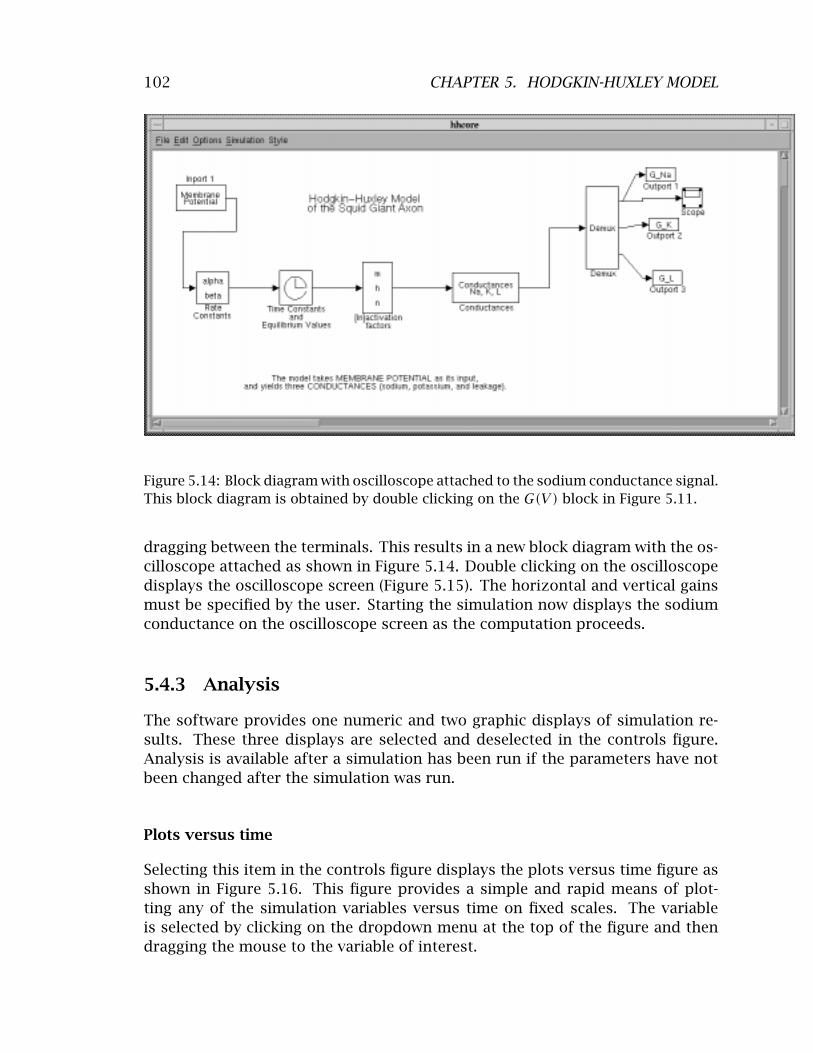
102 CHAPTER 5. HODGKIN-HUXLEY MODEL
Figure 5.14: Block diagram with oscilloscope attached to the sodium conductance signal. This block diagram is obtained by double clicking on the G(V ) block in Figure 5.11.
dragging between the terminals. This results in a new block diagram with the oscilloscope attached as shown in Figure 5.14. Double clicking on the oscilloscope displays the oscilloscope screen (Figure 5.15). The horizontal and vertical gains must be specified by the user. Starting the simulation now displays the sodium conductance on the oscilloscope screen as the computation proceeds.
5.4.3 Analysis
The software provides one numeric and two graphic displays of simulation results. These three displays are selected and deselected in the controls figure. Analysis is available after a simulation has been run if the parameters have not been changed after the simulation was run.
Plots versus time
Selecting this item in the controls figure displays the plots versus time figure as shown in Figure 5.16. This figure provides a simple and rapid means of plotting any of the simulation variables versus time on fixed scales. The variable is selected by clicking on the dropdown menu at the top of the figure and then dragging the mouse to the variable of interest.

103 5.4. USER’S GUIDE TO THE SOFTWARE
Figure 5.15: The oscilloscope screen showing a plot of the sodium conductance which is displayed as the computation proceeds.
Figure 5.16: The plot versus time figure with Vm chosen for plotting.

104 CHAPTER 5. HODGKIN-HUXLEY MODEL
Figure 5.17: The variable summary figure after the simulation has been completed using the default parameters for a current-clamp configuration.
Variable summary
Selecting this item in the controls figure displays the variable summary figure as shown in Figure 5.17. This figure contains four columns of text. The first column identifies the simulation variable. The second contains the initial value of the variable. The third and fourth columns contain the minimum and maximum values of the variables during the course of the simulation.
Comparison
Selecting this item in the controls figure displays the comparison figure as shown in Figure 5.18. This flexible graphic resource is described more fully in Chapter 1. Briefly, this figure allows plotting any result of the simulation against any other in coordinates chosen by the user. Several dependent variables can be plotted simultaneously. In addition, results saved in files can be plotted so that results for different parameters can be compared. In addition, results of consecutive simulations can be overlayed. We give a few examples of the types of graphics that are readily available with this resource.
As shown in Figure 5.19, parametric plots of one variable versus another with time as the parameter are easily obtained. Figure 5.20 shows the membrane potential obtained at several different temperatures. This figure was obtained by overlaying successive computations. It could also have been created by saving the results of simulations performed for different temperatures in files and then plotting the results from these files.

105 5.4. USER’S GUIDE TO THE SOFTWARE
Figure 5.18: Comparison figure showing the membrane potential and ionic conductance obtained from a simulation with model parameters and the stimulus defined in Figures 5.4 and 5.7.

106 CHAPTER 5. HODGKIN-HUXLEY MODEL
Figure 5.19: Phase-plane plot of membrane conductances versus membrane potential during an action potential. All the parameters were the default parameters shown in Figure 5.4 and the stimulus was the same as shown in Figure 5.7 except that the duration was increased to 20 ms.

107 5.4. USER’S GUIDE TO THE SOFTWARE
Figure 5.20: Membrane potential obtained at different temperatures. All the parameters were the default parameters shown in Figure 5.4 except for the temperature and the stimulus was the same as shown in Figure 5.7.

108 CHAPTER 5. HODGKIN-HUXLEY MODEL
5.4.4 Scripting
As mentioned in the Introductory chapter, some of the software packages lend themselves to user written scripts that automate a sequence of computations. The following is an example of a script used to perform current clamp simulations at different temperatures.
%A Hodgkin-Huxley script demonstration%(contents are in HHDEMO1.M)
%This script can be used to generate simulation data using the%current-clamped configuration. The temperature is varied while%all other parameters remain unchanged.
%With each setting of the temperature, the simulation is run%and the resulting data are saved to data files which can then be%used to display the results in the Comparison figure.
%Before using the script, make sure that the Hodgkin-Huxley%biophysics software has been started.%If it hasn’t been started, start the software using SOFTCELL.M% softcell(’hh’);
%hhscr(’set’) will list the parameters that can be changed%The parameter names are case-sensitive, so make sure that%you type them exactly as shown.
%Insure that the current clamped configuration is being used.hhscr(’set’,’Configuration’,’Current clamped’);
%Since a lot of files will be created, it is best to store%them in a separate folder.foldername = pwd;
%Examples of foldername are%foldername = ’C:\data\temp’;%foldername = ’/user/tsb/data/temp’;
%Make sure that a separator character ends the pathnamepathname = tfname(foldername);
%Set up a loop that samples through a temperature range.%In this case, we use the range T = [0 10 20 30] Celsiusfor temp = 0:10:30

109 5.5. PROBLEMS
%set the model’s temperature parameternewtemp = hhscr(’set’,’T_C’,temp);
%perform simulationhhscr(’start’);
%give yourself a note: indicate in the console what the%settings aredisp([’Temperature is set to ’ num2str(newtemp)]);
%create a unique filename that contains the simulation datafilename = [’temp’ num2str(temp) ’.mat’];
%save the simulation data to the file hhscr(’save’,’simulation’,filename,pathname);
end
%That’s it -- all the data have been saved.
%Now, put up all the data simultaneously by following these steps:%1. call up the "Comparison plots" figure,%2. insure that the "Use data files" radiobutton is on,%3. using "Select x,y", select whichever variable(s) to plot,%4. use "Graph x,y" in the "Comparison plots" figure to view all% the data.
5.5 Problems
Problem 5.1 Use the default parameters of the Hodgkin-Huxley model under voltage-clamp conditions to complete the following problems. You may change only the stimulus parameters.
a. The potassium conductance
i. Find the amplitude and duration of a rectangular pulse of membrane potential such that the potassium conductance reaches its final of GK(Vm, �) = 9 ± 0.2 mS/cm2.
ii. What is the value of the time constant of n, �n, during this pulse?
b. The sodium conductance
i. Find the amplitude and duration of a rectangular pulse of membrane potential such that the peak sodium conductance is 15 ± 0.2 mS/cm2.

�
110 CHAPTER 5. HODGKIN-HUXLEY MODEL
Make sure that the pulse duration is sufficient so that there is a peak in the sodium conductance before the pulse terminates.
ii. What are the values of m and h at the time of the peak value of the sodium conductance?
iii. Increase the amplitude of the pulse 20 mV from the value you found above and determine the peak sodium conductance and the values of m and h at the time of the peak value of the sodium conductance.
iv. Decrease the amplitude of the pulse 20 mV from the value you found above and determine the peak sodium conductance and the values of m and h at the time of the peak value of the sodium conductance.
Problem 5.2 This problem deals with the differences in time dependence of the [in]activation factors in voltage-clamp and current-clamp experiments.
a. Run the simulation in the voltage-clamp configuration using the default parameters, except delay the onset of the pulse of voltage by 1 ms to make the on and off transients more readily visible. Examine the results of the simulation and answer the following questions.
i. Describe and explain the dependence on time of �m, m�, and m.
ii. Describe and explain the dependence on time of �h, h�, and h.
iii. Describe and explain the dependence on time of �n, n�, and n.
iv. Plot the voltage dependence of �m, �h, �n, m�, h�, and n . Check the numerical values of these variables against those obtained in parts i, ii, and iv.
b. Run the simulation in the current-clamp configuration using the default parameters. Examine the results of the simulation and answer the following questions.
i. Describe and explain the dependence on time of �m, m�, and m.
ii. Describe and explain the dependence on time of �h, h�, and h.
iii. Describe and explain the dependence on time of �n, n�, and n.
c. Succinctly summarize the differences in the time dependence of all these variables in voltage-clamp and current-clamp configurations.
Problem 5.3 In this problem we illustrate another useful aspect of performing simulation experiments on the model; the model can be used to test ideas concerning proposed measurements on cells.
Assume that the membrane of neuron X has voltage-current characteristics as described by the Hodgkin-Huxley model except that the voltage dependences

�.
�
111 5.5. PROBLEMS
of the parameters of the factors n, m, and h are unknown. In this problem you are asked to develop methods to estimate the voltage dependence of some of these parameters and to assess the accuracy of your methods. To make the simulations realistic, in all parts of the problem you may only change the following parameters: the concentrations of sodium, potassium, and calcium either inside or outside the cell, and the temperature. You may use either voltage-clamp experiments or current clamp experiments. You can choose any stimulus waveform that you can construct with the simulation. However, you must base your estimation method on the membrane current in voltage clamp experiments and/or on the membrane potential in current-clamp experiments. For example, you cannot base your estimation method on a direct measurement of m(t).
a. Develop a method to estimate the voltage dependence of m�. Use the simulation to assess the accuracy of your method by comparing the results of your estimation of m� with a direct computation of m
b. Develop a method to estimate the voltage dependence of h . Use the simulation to assess the accuracy of your method as in part a.
Problem 5.4 By changing the amplitude of the stimulus pulse, while keeping all other parameters at their default values, determine the threshold of the action potential to a precision of 4 significant digits.
a. Describe the changes in action potential waveform as a function of current amplitude.
b. Does the change in waveform of the action potential as a function of stimulus amplitude violate the all-or-none principal? Explain.
c. Investigate the basis of the change in waveform of the action potential by examining the behavior of variables in addition to the membrane potential as the current amplitude is varied.
Problem 5.5 Examine the refractory properties of the model by applying two current pulses, each of amplitude 30 µA/cm2 and duration 0.5 ms and separated by 12 ms in time. Set the simulation duration to 20 ms. Run the simulation. You should observe two action potentials. Reduce the inter-pulse interval to 10 ms. What happens? Now change the amplitude of the second pulse to 50 µA/cm2
and observe the response. Change the inter-pulse interval to 5 ms and observe the outcome.
a. Have you observed properties of the absolute or the relative refractory period?

112 CHAPTER 5. HODGKIN-HUXLEY MODEL
b. By examining the behavior of the factors m, n, and h during these two-pulse simulations, determine which of these factors are most influential in refractory properties.
Problem 5.6 Observe the phenomena of repetitive activity and depolarization block by performing a sequence of simulations with the following parameters. Use a single current pulse of duration 40 ms, a simulation duration of 50 ms, and stimulus amplitudes of 10, 25, 50, 100, and 200 µA/cm2.
a. Note that both the number of action potentials and their amplitudes vary with the current amplitude. Sketch the relation between the number of action potentials and current amplitude and between action potential amplitude and current amplitude.
b. By examining the behavior of the factors m, n, and h determine which of these factors are most influential in determining repetitive activity. Explain your reasoning.
Problem 5.7 The phenomenon of anode-break excitation can be demonstrated by applying a pulse of current of duration 20 ms and amplitude −20 µA/cm2. Use a simulation duration of 40 ms.
a. Why is this phenomenon called anode-break excitation?
b. By exploring the model variables explain this phenomenon.
Problem 5.8 The phenomenon of accommodation can be illustrated by applying a ramp of current of slope 0.4 µA/(cm2 ms) starting at an amplitude of 0 for a · duration of 6 seconds (also set the simulation duration to 6 seconds). The model
¯does not show accommodation for the default value of GNa 120 mS/cm2 but= does for a value of 80 mS/cm2. When the simulation is completed, plot the sodium, potassium and membrane current versus the membrane potential.
a. Perhaps no action potential has occurred in response to the ramp of current because the reduced value of the sodium conductance prevents action potential from being generated for any stimulus. Test this hypothesis.
b. Explain the underlying basis of accommodation.
c. What does the phenomenon of accommodation suggest about the notion of the threshold for eliciting an action potential?
Problem 5.9 Sub-threshold oscillations can be observed by using the default parameters with current pulses of 50 ms duration and simulation durations of 100 ms. Use current amplitudes of .01, .1, 1, 2, and 2.5 µA/cm2.
5.5. PROBLEMS 113
a. Describe your observations.
b. Can the response of the model to a step of current be represented by the response of a network consisting of a constant resistance in parallel with a constant capacitance. Explain.
c. If your answer to part b was no, then devise a current stimulus such that the model’s response will approximate that of a network consisting of a constant resistance in parallel with a constant capacitance. Explain your method.
Problem 5.10 Determine the threshold current amplitudes (to three significant figures) for eliciting action potentials for current pulses of duration 0.01, 0.05, 0.1, 0.5, 1, 2, 5, 10, and 20 ms.
a. How does the threshold depend on current duration for low durations? Explain this behavior.
b. How does the threshold depend on current duration for long durations? Explain this behavior.
Problem 5.11 The Hodgkin-Huxley model with the default parameters stimulated by a pulse of membrane current of amplitude 20 µA/cm2 and of duration 0.5 ms produces an action potential as shown in Figure 5.21. In each of the following computations, one membrane parameter only differs from the default parameters, and for each of these computations no action potential occurs. The parameter changes are:
i. A change in the temperature from 6.3� C to 35� C blocks the action potential as shown in Figure 5.21.
ii. A change in the maximum potassium conductance from 36 to 72 mS/cm2
blocks the action potential. [Results not shown.]
iii. A change in the internal calcium concentration from 0.0001 to 0.0002 mmole/l blocks the action potential. [Results not shown.]
iv. A change in the membrane capacitance from 1 µF/cm2 to 20 µF/cm2 blocks the action potential as shown in Figure 5.21.
v. A change in the external calcium concentration from 44 mmole/l to 22 mmole/l blocks the action potential. [Results not shown.]
Examination of the results for the above computations (e.g., Figure 5.21) reveals that there is no large change in membrane potential, i.e., no action potential has occurred. For each of the computations:
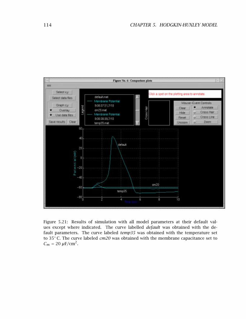
114 CHAPTER 5. HODGKIN-HUXLEY MODEL
Figure 5.21: Results of simulation with all model parameters at their default values except where indicated. The curve labelled default was obtained with the default parameters. The curve labeled temp35 was obtained with the temperature set to 35� C. The curve labeled cm20 was obtained with the membrane capacitance set to
20 µF/cm2.Cm =

5.6. PROJECTS 115
a. Explain why no action potential occurred. You may wish to base your explanation on the results obtained with each of the above computations. For example, you may wish to examine the membrane currents, conductances, and activation variables that occurred for each computation. You may also wish to perform additional computations using different model parameters. For example, to see why no action potential occurs for a large temperature change, it might be instructive to examine the effects produced by smaller changes in temperature. Since for many of the parts of this problem, there are large changes in parameters you may wish to explore the role of the numerical methods in arriving at the solutions.
b. Determine a set of parameters so as to produce an action potential with a waveform that is identical, except for a change in time scale and a change in resting potential, to the action potential obtained with the default parameters. However, for each of the above parts, you may not change the parameter that differs from its default value. For example, for computation in part i, you may not change the temperature. Your task is to change some other parameter or group of parameters such that the action potential is restored. For computation in part ii, you may not change the maximum potassium conductance. For computations in parts iii and v, you may not change either the internal or the external calcium concentration, etc. REMEMBER — the objective is not just to produce an action potential, that is too easy, but to obtain an action potential whose waveform is identical to that obtained with the default parameters. To determine whether or not the action potential is identical to that obtained with the default parameters, you can superimpose plots and/or look at the variables summary figures from the responses. You should use the computer as a tool to check your ideas and not as a substitute for thinking. You should avoid a strictly trial-and-error approach. There are simply too many parameters in the Hodgkin-Huxley model for you to explore them all randomly. When you have arrived at a satisfactory solution, print a hard copy of the model parameters figure showing the parameters you used to solve the problem and include this with your solution. Explain why your parameter change produces the desired result. [HINT: simulations are not required to solve these problems, but they are helpful for checking ideas quickly.]
5.6 PROJECTS
The simulation software lends itself to more extensive study than that included in the Problems. These more extensive studies are called Projects and these are described here.

116 CHAPTER 5. HODGKIN-HUXLEY MODEL
5.6.1 Practical considerations in the choice of a topic
Projects can involve almost any of the properties of the Hodgkin-Huxley model. However, to avoid projects whose aims are vague (e.g., “I would like to understand how the Hodgkin-Huxley model works”) the proposed project should be in the form of a specific and testable hypothesis. Projects that involve months of computation should obviously be avoided. Experience should indicate the duration required to run simulations of the Hodgkin-Huxley model. These durations should be taken into account explicitly in planning a project. For example, any project that involves measuring the threshold of occurrence of an action potential for many different parameter values is bound to be very time consuming, because determining the threshold for a single set of parameters itself involves many computations. The task is to choose a physiological property of the excitation of the action potential that is of interest, and then to define a specific, feasible project.
5.6.2 Choice of topics
Topics can involve comparing predictions of the Hodgkin-Huxley model with measurements on cells. For example, the effects of changes in sodium ion concentration on the action potential have been measured (Hodgkin and Katz, 1949a; Baker et al., 1961). A project might involve reading the original papers that describe such measurements (some were made before the Hodgkin-Huxley model was formulated), and testing the hypothesis that these measurements are (or are not) consistent with the Hodgkin-Huxley model. Similarly, a project might involve examining the effect of some pharmacological substance on measurements of the action potential and testing the hypothesis that the substance produces its effect by changing one or another parameter of the model. These projects will require some reading of original literature which is often difficult and usually time consuming. However, such a project can lead to a very rewarding educational experience. Alternatively, the project might involve a purely theoretical topic in which some property of the model is explained in terms of the underlying structure of the model. This type of project does not necessarily involve reading the original literature. To make the process of project definition more tangible, we shall discuss one property of the Hodgkin-Huxley model of a space-clamped axon, the shape of the action potential, and suggest some appropriate projects based on this property.
Background
The waveform of the action potential is different in different types of electrically-excitable cells. As demonstrated in Figure 5.22, while the action potential waveform has a peak-to-peak amplitude of about 100 mV, the duration and time course vary greatly. It is also known that the action potential waveform of a cell can

117 5.6. PROJECTS
+50
Squid giant axon
Electric eelelectroplaque
+50
0 0
−50 −50
−100 −100
0 4 8 0 3 6 9Time (ms) Time (ms)
+50
Mem
bra
ne
pot
enti
al (
mV
)
Catmotoneuron
Frog sartoriusmuscle fiber
+50
0 0
−50 −50
−100
0 4Time (ms)
+50
0
−50
−100
−100
8 0 10 20 30 Time (ms)
+50
0
-50
−100
Cat myelinated fiber
Sheep purkinje fiber
0 1 2 0 0.5 1 1.5Time (ms) Time (s)
Figure 5.22: Examples of action potentials measured in a variety of cell types (Keynes and Aidley, 1991, adapted from Figure 2.4).

118 CHAPTER 5. HODGKIN-HUXLEY MODEL
20.2
32.5
13.3 9.8
6.3
3.6V m (t
) − V m o
(mV
)
50
0
100
0 1 2 3Time (ms)
Figure 5.23: Dependence of the action potential on temperature for measurements obtained from a giant axon of the squid (Hodgkin and Katz, 1949b).
0 1 2 3 4
0
40
-40
-80
Mem
bra
ne
pot
enti
al (
mV
)
Time (ms)
1
2 3
Figure 5.24: Effect of extracellular sodium concentration on the membrane potential of a giant axon of a squid (Hodgkin and Katz, 1949a, adapted from Figure 4). Traces 1 and 3 are the action potentials obtained in normal sea water before and after trace 2 which was obtained in sea water with 50% sodium content. Isotonic solutions were obtained by using mixtures of sea water and a glucose solution.
be changed by changing a number of experimental variables. For example, increasing the temperature tends to decrease the duration of the action potential (Figure 5.23), and reducing the external sodium concentration reduces the amplitude and increases the duration of the action potential (Figure 5.24). Since action-potential waveforms vary from cell to cell and vary for one cell if environmental variables are changed, this raises a question — To what extent are changes in action-potential waveforms seen in different cells due to inherent differences in the membrane mechanisms rather than to differences in membrane parameters with identical membrane mechanisms? For example, the action potentials of the squid axon and the frog and rat nodes of Ranvier shown in Figure 5.22 were measured at different temperatures. In fact, the briefest action potentials were obtained at the highest temperatures. Since Figure 5.23 indicates that the duration of the action potential does become shorter at higher temperatures in squid axon, it may be that the temperature differences in the measurements could explain the differences in the waveforms of the action potentials of these three preparations. It is clear that temperature changes alone cannot explain all the

119 5.6. PROJECTS
variations seen in Figure 5.22 since the long-duration action potential of frog cardiac muscle was obtained at a higher temperature than was the action potential of the squid giant axon. However, perhaps some combination of changes of parameters in addition to temperature (e.g., ion concentrations, ion conductances, membrane capacitance, etc.) might explain the long-duration action potential of cardiac muscle.
Examples of hypotheses
The list of projects given below includes a number that deal with the waveform of the action potential generated by the Hodgkin-Huxley model as well as a few that deal with other topics.
1. Hypothesis — The difference in waveform of the action potential of a frog node of Ranvier and of a squid giant axon (Figure 5.22) can be reproduced by the Hodgkin-Huxley model of a squid giant axon by a change in temperature.
2. Hypothesis — The membrane capacitance determines the time course of the rising phase of the action potential. Increasing the membrane capacitance decreases the rate of increase of the rising phase of the action potential.
3. Hypothesis — The falling phase of the action potential (repolarization) can occur in the absence of a change in potassium conductance.
4. Hypothesis — Increasing the temperature sufficiently blocks the occurrence of the action potential because the membrane time constant limits the rate at which the membrane variables can change and prevents the difference in time course of the sodium and potassium activation which is responsible for initiation of the action potential.
5. Hypothesis — The initiation of the action potential is independent of the potassium conductance.
6. Hypothesis — The prolonged plateau of the cardiac muscle action potential can be accounted for by the Hodgkin-Huxley model with a potassium conductance that has a slow activation.
7. Hypothesis — The effect of tetraethylammonium chloride (TEA) on the action potential of the squid giant axon can be modelled with the Hodgkin-Huxley model by decreasing Kn and increasing Kh. Articles in the literature should be consulted for this project (Armstrong, 1966; Armstrong and Bin-stock, 1965; Tasaki and Hagiwara, 1957).
8. Hypothesis — The shape of the action potential in the presence of tetraethylammonium chloride (TEA) can be accounted for by the Hodgkin-Huxley
120 CHAPTER 5. HODGKIN-HUXLEY MODEL
model with a reduced maximum value of the potassium conductance. Articles in the literature should be consulted for this project (Armstrong, 1966; Armstrong and Binstock, 1965; Tasaki and Hagiwara, 1957).
9. Hypothesis — Increasing the external calcium concentration will block the occurrence of the action potential because this will reduce the difference in the time constant of sodium and potassium activation which is responsible for the initiation of the action potential.
10. Hypothesis — Increasing the external concentration of potassium will decrease the refractory period; decreasing this concentration will lengthen the refractory period.
11. Hypothesis — Increasing the external concentration of sodium will decrease the refractory period; decreasing this concentration will lengthen the refractory period.
12. Hypothesis — Absolute and relative refractory periods are decreased by increasing the rate constants for sodium inactivation and for potassium activation.
13. Hypothesis — Repolarization cannot occur if the potassium activation rate constant is zero.
14. Hypothesis — The threshold of the action potential to a brief pulse of current decreases as the external potassium current is increased.
15. The Hodgkin-Huxley model with default parameters does not exhibit accommodation (Weiss, 1996b). Hypothesis — Accommodation occurs if the leakage conductance is increased.
16. The Hodgkin-Huxley model with default parameters does not exhibit accommodation (Weiss, 1996b). Hypothesis — Accommodation occurs if the potassium conductance is increased.
17. Hypothesis — Increasing the leakage equilibrium potential will block the action potential.
18. Hypothesis — The effect of the changes in concentration of sodium ions on the action potential of the giant axon of the squid can be accounted for by the Hodgkin-Huxley model. Articles in the literature should be consulted for this project (Hodgkin and Katz, 1949a; Baker et al., 1961).
19. Hypothesis — In response to rectangular pulses of current, the rheobase of the strength-duration relation increases as temperature increases.
20. Hypothesis — An increase in temperature results in a decrease in the duration of the refractory period.

121 5.6. PROJECTS
21. Hypothesis — The threshold membrane potential at which the Hodgkin-Huxley model produces an action potential in response to a brief pulse of current is equal to the membrane potential for which the linearized Hodgkin-Huxley equations have unstable eigenvalues.
22. Application of a long-duration constant current to the Hodgkin-Huxley model produces a train of action potentials. Hypothesis — The frequency of the action potentials increases with increasing current amplitude.
23. Application of a long-duration constant current to the Hodgkin-Huxley model produces a train action potentials. Hypothesis — The frequency of action potential increases as the parameter Kn is increased.
24. Application of a long-duration constant current to the Hodgkin-Huxley model produces a train action potentials. Hypothesis — The frequency of action potential increases as the temperature is increased.
25. Hypothesis — An increase in the external concentration of potassium increases the threshold potential at which an action potential is elicited.
26. Hypothesis — Increasing Kh will result in an increase in the steepness of the repolarization phase of the action potential.
Any of these (or other) hypotheses can be the starting point for a project. Most of the hypotheses given above are simplistic, and a careful investigation will reveal their shortcomings. The Hodgkin-Huxley model is sufficiently complex that investigation of any of the hypotheses will most likely lead to unexpected results. You should pursue these unexpected results and try to understand their bases. For example, you may find that in pursuing some hypothesis you choose to change some parameter of the model that you expect to result in some change in action potential waveform. The resulting computation might reveal, much to your surprise and chagrin, that no action potential has occurred. Determine why no action potential occurred. The explanation will usually be instructive. Your aim should be not simply to reject or accept the hypothesis but to delve into the topic in sufficient depth so as to a deepen your understanding of the model. One outcome of the project might be to restate your original hypothesis in a new and more sophisticated form.
Beginning with the proposal and extending through the project, you should keep clearly in mind that you are not investigating nerve membrane. You are investigating the Hodgkin-Huxley model for the membrane of the squid giant axon. Your explanations of all phenomena must be in terms of the primitive concepts of this model — the ionic conductances, ionic concentrations, ionic currents, the capacitance, and the variables m, n, and h. Explanations in terms of molecular channel mechanisms or electrodiffusion of ions in the membrane or ion pumps are irrelevant in so far as they are not contained in the Hodgkin-Huxley model!
122 CHAPTER 5. HODGKIN-HUXLEY MODEL
5.6.3 The proposal
The proposal should contain a brief statement of the hypothesis you propose to test, as well as your proposed method of procedure. Include a list of the computations you will perform and the measurements you plan to make. Indicate how the measurements will be used to help you come to a conclusion. The proposal should be written on one 8 1/2 × 11 sheet of paper. A sample proposal is shown in Figure 5.25.
5.6.4 The computations
After carefully defining the computations needed to determine the validity of your hypothesis, you should perform the necessary computations. You should keep careful track of the computations you perform by entering relevant information in a notebook. The notebook should indicate the date of each computational session as well as the identity of the computer you used (make and model). Keep an accurate record of each computation so that you can reconstruct what you did at a later date. Save your results in files. Make composite plots to summarize a series of measurements. For example, to show the effect on the action potential of some parameter, plot the action potentials for selected values of the parameter on one set of axes. Arrange you work so that you have time for some final computations after you begin writing the report. You may find that new questions will arise as you write the report. If you leave adequate time, you may be able to resolve these questions.
5.6.5 The report
The report is an opportunity for you to work on your ability to express yourself succinctly. Your report should contain text, figures, tables, etc. whatever you need to make your point most effectively. Assume that the background of your readers is that of the students and faculty in your class.
Your report should contain several sections.
Hypothesis
Briefly restate your original hypothesis.
Rationale
Briefly explain your approach to testing your hypothesis. In broad terms, explain what you did to test your hypothesis and why you did it.

123 5.6. PROJECTS
PROPOSAL: HODGKIN-HUXLEY MODEL PROJECT
Name: Hy I.Q. Student •
Email address: hiqstudent•
Hypothesis: The difference in observed action potential shape between • the giant axon of the squid and the node of Ranvier of the rat is due to a difference in temperature.
Background: The rate constants that determine the variables m, n, and • h in the Hodgkin-Huxley model increase as the temperature is increased. Hence, I would expect that with increased temperature the time course of the action potential would be briefer. The observed action potential of the rat node of Ranvier measured at 37�C. is briefer than the action potential of the squid giant axon measured at 16�C. Hence, I will determine whether this difference in temperature is adequate to explain the difference in action-potential waveform. In this study, I will assume that the Hodgkin-Huxley model accounts for action potentials in both preparations. Since the intracellular and extracellular ionic concentrations of sodium, potassium and calcium also differ in these two preparations, if time permits I will also investigate the effect of this difference.
Procedure: I will obtain the intracellular and extracellular concentrations of • sodium and potassium ions for the rat node of Ranvier from the literature. I will perform a series of simulation studies with a single pulse of membrane current whose amplitude will be set at a constant suprathreshold value. I propose the following series of simulations
# Temp. Ion Concentrations
�C
1 16 default values for squid giant axon
2 37 default values for squid giant axon
3 16 values found for rat node
4 37 values found for rat node
The waveforms of the action potentials obtained under the various conditions will be compared on the graphics display and the summary statistics for each condition will be examined. If condition 4 yields an action potential that resembles that which is measured on the rat node of Ranvier, then the hypothesis will be supported by these calculations. If they differ, then I will investigate the bases of the differences.
Figure 5.25: Sample proposal for a project.

124 CHAPTER 5. HODGKIN-HUXLEY MODEL
Methods and procedures
In this section you should explain any methodological or procedural issues. For example, if you measured the time of the peak of the action potential as a function of some parameter, explain how you measured the time of the peak and how you defined when an action potential occurred, i.e., how did you separate the action potential from the local response.
Results
Describe your computational results and provide documentation such as that shown in Figures 5.18-5.20, as well as summary plots and tables. This section should be organized to lead the reader through a logical sequence of results that terminates inexorably in a conclusion. Your objective is to construct an airtight case for some conclusion whether or not it supports or rejects your original hypothesis. This is not the place to interpret or to discuss your results.
Conclusions and Discussion
State your conclusions concisely and point out how your results support your conclusions. You might also suggest additional computations to further test your hypothesis. Your conclusions and discussion should be focussed on the relation between your results and your hypothesis.
Grade
Your grade on this report will be determined largely by the extent to which you follow the above directions, avoid extraneous and irrelevant discussion, and express your thoughts clearly.

Chapter 6
VOLTAGE-GATED ION CHANNELS
125

126 CHAPTER 6. VOLTAGE-GATED ION CHANNELS
6.1 Introduction
6.1.1 Historical background
Passive transport of ions through cellular membranes is mediated by membrane-bound channel proteins that form selectively permeable ion channels. Although their existence was long suspected, the first direct physiological evidence for these channels became available in 1976 (Neher and Sakmann, 1976). Subsequently, many different types of channels have been identified (Hille, 1992). Channels can be categorized on the basis of the physical/chemical variable that opens or gates the channel. For example, the channels that underlie the properties of electrically excitable cells are gated by the membrane potential and are called voltage-gated channels. These channels are opened by a change in membrane potential. Other channels are gated by the binding of specific chemical substances, mechanical deformation of the membrane, etc. In all of these cases, the channels behave as if they have a discrete number of states, of which a few (usually only one) are conducting or open states and the others (usually more than one) are non-conducting or closed states. The channel switches rapidly and randomly among its allowable states, and the probability that a transition occurs at a particular time depends on the value of the gating variable.
Models of the gating of single ion channels were developed almost immediately after single-channel data were obtained (Colquhoun and Hawkes, 1977). Descriptions of these models can be found elsewhere (Colquhoun and Hawkes, 1995a; Weiss, 1996b).
6.1.2 Overview of software
This software package enables users to enhance their understanding of models of the gating of single voltage-gated ion channels. The software allows the user to design a channel by choosing the number of states, the voltage dependence of transitions between states, the conductance and gating charge of each state, and the equilibrium potential for the channel. After the channel is designed, the user can analyze the behavior of the channel to a change in membrane potential. Any of the variables associated with the channel can be displayed including the state occupancy probability, conductance, ionic current, gating charge, and gating current. Both random variables and their expected values can be displayed as a function of time. The software is sufficiently powerful and flexible to allow users to synthesize realistic, state-of-the-art models for the gating of voltage-gated ion channels.

6.2. DESCRIPTION OF THE MODEL 127
6.2 Description Of The Model
A brief description of the channel model is given here; a more complete description is given elsewhere (Weiss, 1996b). We assume that a channel has N states and that at each instant in time t, the channel is found in one of its states (Figure 6.1). The states are enumerated as {S1, S2, S3, . . . SN }. Each state has state at-
S1 S2 S3 S4
S5
�12 �23 �34
�45�51
�21 �32 �43
�54�15
�1, Q1 �2, Q2 �3, Q3 �4, Q4
�5, Q5
Figure 6.1: Kinetic diagram of a channel that has 5 states. The states are shown linked by rate constants for transitions between states, where τij is the rate of transition from state i to state j. When the channel is in state j the conductance of the channel is γj and the gating charge of the channel is Qj .
tributes: the state conductance and the state gating charge. The state attributes for these states are denoted as {γ1, γ2, γ3, . . . γN } for the state conductances and {Q1, Q2, Q3, . . . QN } for the state gating charges. Given the membrane potential Vm
and the equilibrium potential Veq, the state ionic currents are {I1, 2, 3, . . . N }.I I IThus, when the channel is in state Sj , the state conductance is γj , the state ionic current is j γj(Vm − Veq), and the state gating charge is Qj . Gating currents I = occur at the transitions of the gating charge.
The temporal evolution of the electrical properties of a channel depend upon the state occupancy probabilities which we discuss briefly. Define the probability that the channel is in state j at time t as xj(t), and the transition probability that the channel is in state j at time t + �t given that it was in state i at time t as yij(t + �t). The fundamental assumption of the model for state transitions is that the transition probabilities depend on the present state of the channel and not on previous states. Such a probabilistic process is called a Markov process. Formally, we assume that
yij(t + �t) = τij�t + o(�t) ,
where o(�t) has the property that lim�t≤0 o(�t)/�t 0 and τij is a rate con= stant for transitions from state i to state j. The first term is the probability of

�
� �
128 CHAPTER 6. VOLTAGE-GATED ION CHANNELS
occurrence of a single transition in the interval of duration �t when this interval is short and the rate of transitions is τij . The second term takes into account the probability of the occurrence of multiple transitions in the interval. For intervals �t that are sufficiently small so that no more than one transition is likely to occur in the interval, the o(�t) term is negligible; we will ignore this term in the development that follows. The probability that the channel is in state j at time t +�t and in state i at time t is yij(t +�t)xi(t) √ τijxi�t.
The increase in probability that the channel is in state j in the time interval (t, t + �t) is xj(t + �t) − xj(t). In this time interval, this probability increases as a result of transitions from states i into state j and decreases as a result of transitions from state j into state i. By collecting all such terms we obtain,
N⎩N
xj(t +�t) − xj(t) √ τijxi(t)�t − τjixk(t)�t , i 1,i i 1,i= →=j = →=j
where the first summation is due to transitions into state j and the second sum-
⎩
jmation is due to transitions out of state If we rearrange the terms and take. the limit as �t ≤ 0, we obtain the differential equation
N⎩
dt = i 1,i= →=j
N⎩ τijxi(t) − τjixj(t). (6.1)
i
dxj(t)
1,i →=j=
This equation can be written in matrix form by defining the matrix of transitionprobabilities to be
��������⎤
τ11 τ12 τ1N· · ·
τ21 τ22 τ2N· · ·
· · · · · · · · · · · ·
τN1 τN 2 τNN· · ·
⎪⎪⎪⎪⎪⎪⎪⎪⎣
.=
where τij is the transition rate from state i to state j when i →= j, and τii is�Nchosen so that i 1 τij 0. The state occupancy probability satisfies the matrix = = differential equation
dx(t) x(t)�, (6.2)
dt =
where x(t) is a row matrix of state occupancy probabilities. In addition, since the channel is in one of its N states at each instant in time,
N⎩ xj(t) = 1 .
1j=
The equilibrium state occupancy probability can be obtained directly from Equation 6.2 by setting dx(t)/dt = 0 to yield
0 x(�)�, (6.3)=

� � ���
129 6.2. DESCRIPTION OF THE MODEL
to obtain the equilibrium state occupancy probability x(�). If the matrix � is constant, then the solution to the matrix equation for the
state occupancy probability is (Colquhoun and Hawkes, 1995a)
x(t) = x(0)e�t,
where x(0) is the matrix of the initial value of x(t). Evaluation of the exponential matrix yields the result
N
x(t) = x(0) Sjeφjt, (6.4) j=
where φj is the jth eigenvalue of and Sj is the jth spectral matrix of �. Therefore, we see that the state occupancy probabilities are weighted sums of exponentials whose exponents are the eigenvalues of the transition rate matrix. Because the � matrix is singular, one eigenvalue has value zero. All other eigenvalues have negative real parts (Cox and Miller, 1965). Thus, the non-zero eigenvalues lead
⎩
1
to solution exponentials that decay with time. For a voltage-gated channel, the transition rates depend explicitly on the mem
brane potential which in turn may vary with time. If the rate constants are assumed to satisfy the theory of absolute reaction rates (Weiss, 1996a; Weiss, 1996b), then they depend exponentially on the membrane potential,
τij(Vm) = AijeaijVm if i � j,
0 if i = j,
where Aij is a rate factor and aij is an exponential factor. τij(Vm) depends on the membrane potential which in turn depends upon time. Therefore, the rate constants will in general depend upon time.
During intervals of time when the membrane potential is a constant, Equation 6.2 is a linear, first-order matrix differential equation with constant coefficients. The solution determines the state occupancy probabilities, the {xj(t)}s. The expected values of the channel conductance, channel current, and gating charge are computed directly from the state occupancy probabilities. If the conductance of the channel is γj when the channel is in state j, then the expected value of the conductance of the channel, g(t), is
N⎩ g(t) = γjxj(t). (6.5)
1j=
If we assume that the current through the channel when the channel is in state j is γj(Vm − Veq), the expected value of the single-channel current, i(t), is
N⎩ i(t) = γjxj(t)(Vm − Veq) = g(t)(Vm − Veq). (6.6)
1j=

130 CHAPTER 6. VOLTAGE-GATED ION CHANNELS
Similarly, if the gating charge of the channel when the channel is in state j is Qj , the expected value of the single-channel gating charge, qg(t), is
N⎩ qg(t) = Qjxj(t). (6.7)
1j=
The expected value of the single-channel gating current, ig(t), is
ig(t) = dqg(t) . (6.8)dt
6.3 Numerical Methods
6.3.1 Integration step
The differential equation for the state occupancy probability (Equation 6.2) is solved numerically using methods described elsewhere (Colquhoun and Hawkes, 1995b). The accuracy and efficiency of the numerical solution depends upon the value of the integration step, �t. The value of �t needs to be chosen small enough so that the time rate of change in the occupancy probabilities can be resolved accurately and so that the random variables are represented accurately. The choice of an adequate value of �t depends upon the eigenvalues of the state transition rate matrix. Typically, �t should be chosen so that �t 1/ φmax , where ◦ |φmax is the eigenvalue with the largest magnitude. The smaller
|�t is chosen
the more accurate the integration in any one step, but the longer the computation will take. In addition, long computations can result in the accumulation of round-off errors. Thus, the choice of �t is a compromise between the speed and accuracy of the simulation. Solution of the matrix equation (Equation 6.4) determines the occupancy probabilities of each state. From these probabilities, the expected values of the conductances, currents and gating charge are computed using Equations 6.5-6.8.
Random variables are computed from state transition probabilities. Transitions probabilities from state i to state j are computed from the relation yij(t +�t) √ τij �t at each instant in time. The time interval for computing random variables is set equal to the integration step �t. The occurrence of a transition is determined by a random number generator. The sequence of state transitions determines the sequence of conductance values and gating charges since each state has a unique conductance and gating charge. The conductance values determines the current since this current is determined by specifying the conductance, the membrane potential, and the channel equilibrium potential. The gating current random variable is represented by impulses at the times of transition of the gating charge and whose areas equal the discontinuities in gating charge.
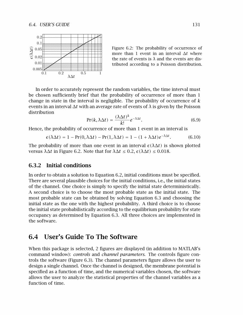
131 6.4. USER’S GUIDE
0.2
0.1
0.05
0.02
0.01
0.005
�(φ�t) Figure 6.2: The probability of occurrence of
more than 1 event in an interval �t where the rate of events is φ and the events are distributed according to a Poisson distribution.
0.1 0.2 0.5 1 φ�t
In order to accurately represent the random variables, the time interval must be chosen sufficiently brief that the probability of occurrence of more than 1 change in state in the interval is negligible. The probability of occurrence of k events in an interval �t with an average rate of events of φ is given by the Poisson distribution
Pr(k, φ�t) = (φ�t)k
e−φ�t. (6.9)k!
Hence, the probability of occurrence of more than 1 event in an interval is
�(φ�t) = 1 − Pr(0, φ�t) − Pr(1, φ�t) = 1 − (1 + φ�t)e−φ�t. (6.10)
The probability of more than one event in an interval �(φ�t) is shown plotted versus φ�t in Figure 6.2. Note that for φ�t ← 0.2, �(φ�t) ← 0.018.
6.3.2 Initial conditions
In order to obtain a solution to Equation 6.2, initial conditions must be specified. There are several plausible choices for the initial conditions, i.e., the initial states of the channel. One choice is simply to specify the initial state deterministically. A second choice is to choose the most probable state as the initial state. The most probable state can be obtained by solving Equation 6.3 and choosing the initial state as the one with the highest probability. A third choice is to choose the initial state probabilistically according to the equilibrium probability for state occupancy as determined by Equation 6.3. All three choices are implemented in the software.
6.4 User’s Guide To The Software
When this package is selected, 2 figures are displayed (in addition to MATLAB’s command window): controls and channel parameters. The controls figure controls the software (Figure 6.3). The channel parameters figure allows the user to design a single channel. Once the channel is designed, the membrane potential is specified as a function of time, and the numerical variables chosen, the software allows the user to analyze the statistical properties of the channel variables as a function of time.

132 CHAPTER 6. VOLTAGE-GATED ION CHANNELS
Figure 6.3: The controls figure after the software is initiated.
6.4.1 Controls
The portion of the controls figure (Figure 6.3) below the menubar is divided into five panels. The setup panel allows the user to select the channel parameters figure (which is used to design the channel), the membrane potential figure (which is used to specify the membrane potential as a function of time), and the numerics figure (which is used to specify the initial conditions and the integration step of the solution). A panel just below the setup panel controls the simulation. The simulation can be started, stopped, paused, or continued. The analysis panel allows display of a variety of the results of a simulation. The log panel contains options for recording log entries of the session and is described in Chapter 1. This message panel is used to send messages to the user.
6.4.2 Channel parameters
After the program is initiated, the channel parameters figure displays the default channel kinetic diagram as shown in Figure 6.4. In general, the user constructs a channel model by editing the default channel model. Editing entails adding new states, adding or modifying rate constants that link the states, assigning ionic conductances and gating charges to states, and assigning an equilibrium potential to the channel model.
Each box in the channel parameters figure (Figure 6.4) represents a particular state of the channel and is given a number from 1 to 8 (a maximum of 8 states is possible). The arrows connecting these states depict the transition rates between states. Each box also contains the ionic conductance of the channel when the channel is in that state; the ionic conductance can be changed by clicking on it’s value and typing the new value into the edit box. The ionic conductance is expressed in picosiemens (pS). A value of zero denotes a non-conducting state. Each box also contains the gating charge valence z of the channel when the channel is in that state; the gating charge valence can be changed by clicking on it’s

133 6.4. USER’S GUIDE
Figure 6.4: The channel parameters figure. The rate constant τ12 has already been defined and is displayed in the message panel at the bottom of the figure.
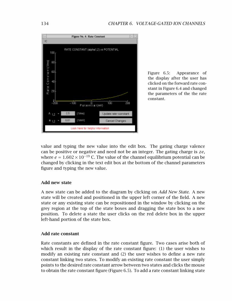
134 CHAPTER 6. VOLTAGE-GATED ION CHANNELS
Figure 6.5: Appearance of the display after the user has clicked on the forward rate constant in Figure 6.4 and changed the parameters of the the rate constant.
value and typing the new value into the edit box. The gating charge valence can be positive or negative and need not be an integer. The gating charge is ze, where e 1.602 × 10⁻¹⁹ C. The value of the channel equilibrium potential can be = changed by clicking in the text edit box at the bottom of the channel parameters figure and typing the new value.
Add new state
A new state can be added to the diagram by clicking on Add New State. A new state will be created and positioned in the upper left corner of the field. A new state or any existing state can be repositioned in the window by clicking on the grey region at the top of the state boxes and dragging the state box to a new position. To delete a state the user clicks on the red delete box in the upper left-hand portion of the state box.
Add rate constant
Rate constants are defined in the rate constant figure. Two cases arise both of which result in the display of the rate constant figure: (1) the user wishes to modify an existing rate constant and (2) the user wishes to define a new rate constant linking two states. To modify an existing rate constant the user simply points to the desired rate constant arrow between two states and clicks the mouse to obtain the rate constant figure (Figure 6.5). To add a rate constant linking state
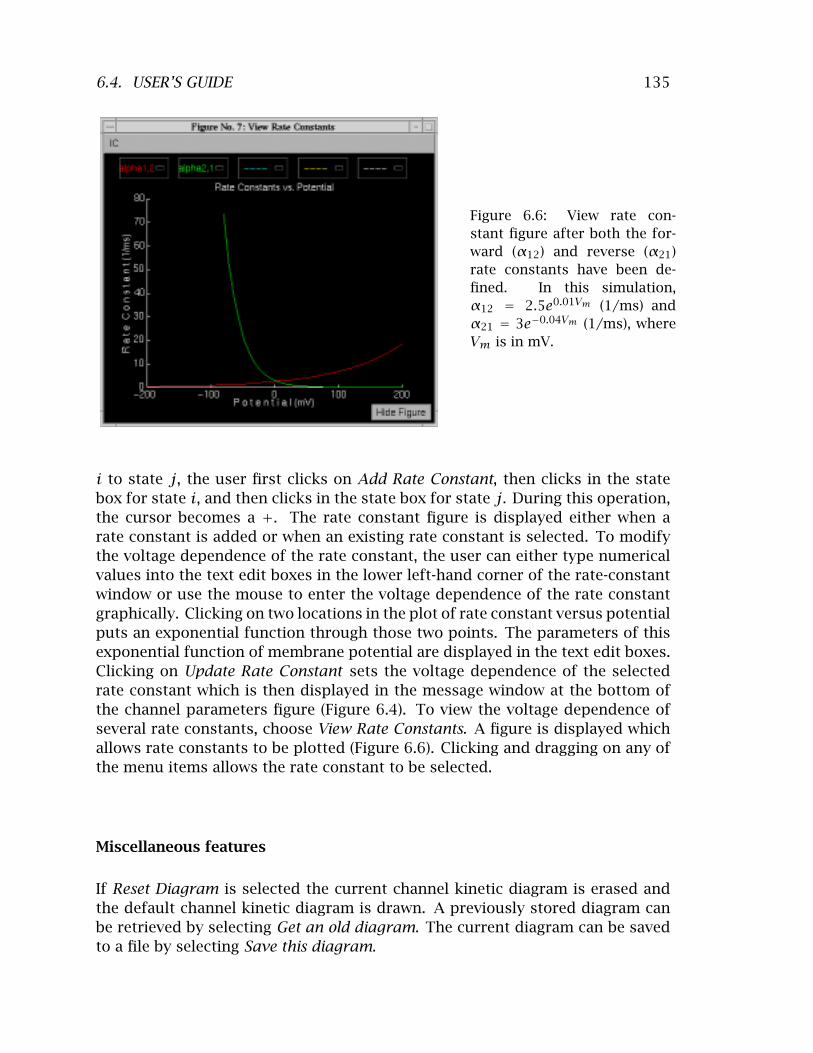
135 6.4. USER’S GUIDE
Figure 6.6: View rate constant figure after both the forward (τ12) and reverse (τ21) rate constants have been defined. In this simulation,
2.5e0.01Vmτ12 (1/ms) and = 3e−0.04Vmτ21 (1/ms), where =
Vm is in mV.
i to state j, the user first clicks on Add Rate Constant, then clicks in the state box for state i, and then clicks in the state box for state j. During this operation, the cursor becomes a +. The rate constant figure is displayed either when a rate constant is added or when an existing rate constant is selected. To modify the voltage dependence of the rate constant, the user can either type numerical values into the text edit boxes in the lower left-hand corner of the rate-constant window or use the mouse to enter the voltage dependence of the rate constant graphically. Clicking on two locations in the plot of rate constant versus potential puts an exponential function through those two points. The parameters of this exponential function of membrane potential are displayed in the text edit boxes. Clicking on Update Rate Constant sets the voltage dependence of the selected rate constant which is then displayed in the message window at the bottom of the channel parameters figure (Figure 6.4). To view the voltage dependence of several rate constants, choose View Rate Constants. A figure is displayed which allows rate constants to be plotted (Figure 6.6). Clicking and dragging on any of the menu items allows the rate constant to be selected.
Miscellaneous features
If Reset Diagram is selected the current channel kinetic diagram is erased and the default channel kinetic diagram is drawn. A previously stored diagram can be retrieved by selecting Get an old diagram. The current diagram can be saved to a file by selecting Save this diagram.

136 CHAPTER 6. VOLTAGE-GATED ION CHANNELS
Figure 6.7: Membrane potential figure after selection of a pulse of potential.
Figure 6.8: Numerics figure appropriate for rate constants shown in Figure 6.6 and membrane potential shown in Figure 6.7.
6.4.3 Membrane potential
Selection of Membrane Potential in the controls figure displays the membrane potential figure (Figure 6.7). The membrane potential can be a rectangular pulse of potential superimposed on a steady holding potential. The user can select the holding potential, the duration of the stimulus, the onset time of the pulse starts, the pulse duration, and pulse amplitude.
6.4.4 Numerics
The numerics figure (Figure 6.8) controls the choice of the integration step and initial conditions for the simulation. The figure consists of four panels. The two upper panels deal with integration steps for the two allowable membrane poten
137 6.4. USER’S GUIDE
tial levels. The next panel down deals with choice of initial conditions (initial states). The final panel is a message window that includes an estimate of the time it will take to complete the simulation for the chosen parameters.
Integration step
For a given choice of membrane potential and voltage-dependent rate constants, the software computes the eigenvalues of the transition rate matrix and displays these results to the user. The smallest time constant is computed from the fastest eigenvalue and the user can choose, by editing the text edit box, to make the integration step a fraction (or a multiple) of this smallest time constant. Alternatively, the user can choose a fixed integration time. The integration time that results from the user’s choice is displayed as is the probability of more than one transition during an interval of time that equals the integration step.
Initial state
The initial state for a simulation can be chosen deterministically to be any of the allowable states or the most probable state for the given initial values of the membrane potential. By default, the initial state is chosen probabilistically by computing the state occupancy probabilities for the chosen initial value of the membrane potential and choosing the initial state randomly using these probabilities.
6.4.5 Analysis
Clicking on the analysis panel of the controls figure allows access to a variety of displays of simulation results including such variables as: the state occupancy, the state occupancy probability, the ionic conductance, the ionic current, the gating charge, and the gating current. Both the random variables and their expected values can be displayed. Ten channels with similar characteristics can be examined simultaneously to allow users to relate macroscopic to microscopic variables. Results of multiple simulations can also be plotted on a single set of axes for the sake of direct comparison.
Three different types of graphs are available. The first type allows plotting a single variable as a function of time in fixed coordinates. An example is the state occupancy figure shown in Figure 6.9. The top panel shows the simulation for 10 independent channels, the middle panel shows the results for channel 1 alone, and the bottom panel shows the state occupancy probabilities for both states of the channel. A second example of this type of graph is the ionic current shown in Figure 6.10. Both the ionic current random variable and its expected value have been selected for plotting. In addition, the average ionic current of 10 identically distributed but statistically independent channels can also be displayed. Similar

138 CHAPTER 6. VOLTAGE-GATED ION CHANNELS
Figure 6.9: State occupancy figure with all variables selected for display.

139 6.4. USER’S GUIDE
Figure 6.10: Single channel ionic current showing the relation between the random variable and its expected value.
plots are available for the ionic conductance, gating charge, and gating current. These displays are helpful for relating macroscopic to microscopic variables and random variables to their expected values.
A second type of graph is the summary graph which allows comparison of the time dependence of channel variables to each other in fixed coordinates (Figure 6.11). Most of the variables are self-evident from the display. However, the representation of the gating current random variable requires some comment. The gating charge random variable is a random rectangular wave. Hence, the gating current random variable, which is defined as the derivative of the gating charge random variable, is a random impulse train (train of Dirac delta functions). We represent these impulses with lollipops. The time of occurrence of a lollipop equals the time of occurrence of an impulse and the height of the lollipop equals the area of the impulse. On the scale of visibility of the gating current random variable, the expected value is often too small to see. Hence, in the plot of the gating current, deselecting the random variable will allow its expected value to be observed. Clicking on the radio button for Cross line displays a vertical line that tracks the position of the mouse cursor. The values of the intersection of the line with each variable is displayed.
The third type of graph allows comparison of results obtained in different simulations in coordinates defined by the user. Clicking on Comparisons in the control figure displays the comparisons figure (Figure 6.12). This figure makes

140 CHAPTER 6. VOLTAGE-GATED ION CHANNELS
Figure 6.11: Summary figure with all variables selected for display.

141 6.4. USER’S GUIDE
Figure 6.12: Comparison figure showing the expected value of the ionic current and of the gating charge for the channel defined in Figures 6.4-6.7.

142 CHAPTER 6. VOLTAGE-GATED ION CHANNELS
use of the graphics package described in detail in Chapter 1.
6.5 Problems
Problem 6.1 This problem deals with a channel that has one two-state gate (which we refer to as a two-state channel) whose rate constants are not a function of membrane potential; this channel is not voltage-gated. Define a two-state channel for which state 1 is closed (nonconducting) and state 2 is open (conducting),
1τ
2 . 21
12�τ
Use rate constants that are constant (independent of membrane potential). In all parts of this problem use rate constants such that τ12 + τ21 = 10 ms−1.
a. Determine opening and closing rate constants such that the channel is equally likely to be in state 1 or state 2.
b. Determine opening and closing rate constants such that the channel is three times as likely to be in state 2 than in state 1.
c. Use the same rate constants as in part b. Set the membrane potential so that it is −50 mV for t < 0.5 ms and +50 mV for t > 0.5 ms. The objective of this part is to design a channel that has a single-channel current when the channel is open ( ) of −1.2 pA when the membrane potential is −50 mV Iand +0.8 pA when it is +50 mV.
i. Determine the equilibrium potential and single-channel conductance when the channel is open (γ). Check your answer by running the simulation using the values of the equilibrium potential and single-channel conductance you determined.
ii. What is the average single-channel current (i) for t < 0.5 ms? What is the average single-channel current for t > 0.5 ms?
Problem 6.2 This problem deals with a two-state channel whose rate constants are functions of membrane potential; the channel is voltage-gated. Define a two-state channel for which state 1 is closed (nonconducting) and state 2 is open (conducting),
1 12�τ
τ2 .
21
Set the membrane potential to −60 mV for t < 0.2 ms and to +40 mV for t > 0.2 ms.
a. Determine voltage-dependent rate constants such that: the channel is closed (with probability > 0.8) for t < 0.2 ms; the channel is open (with probability > 0.8) for t 0.2 ms; and the channel opens with a time constant of about ⇒0.2 ms.
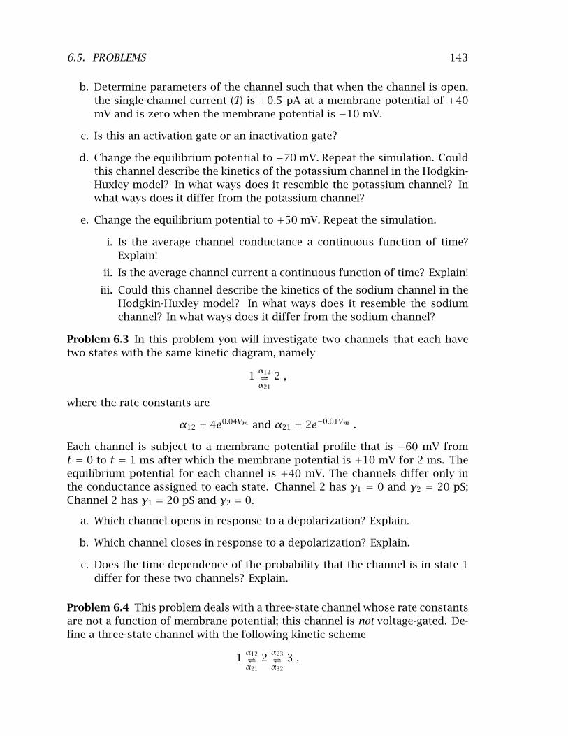
143 6.5. PROBLEMS
b. Determine parameters of the channel such that when the channel is open, the single-channel current ( ) is +0.5 pA at a membrane potential of +40ImV and is zero when the membrane potential is −10 mV.
c. Is this an activation gate or an inactivation gate?
d. Change the equilibrium potential to −70 mV. Repeat the simulation. Could this channel describe the kinetics of the potassium channel in the Hodgkin-Huxley model? In what ways does it resemble the potassium channel? In what ways does it differ from the potassium channel?
e. Change the equilibrium potential to +50 mV. Repeat the simulation.
i. Is the average channel conductance a continuous function of time? Explain!
ii. Is the average channel current a continuous function of time? Explain!
iii. Could this channel describe the kinetics of the sodium channel in the Hodgkin-Huxley model? In what ways does it resemble the sodium channel? In what ways does it differ from the sodium channel?
Problem 6.3 In this problem you will investigate two channels that each have two states with the same kinetic diagram, namely
1τ12�τ21
2 ,
where the rate constants are
τ12 = 4e0.04Vm 2e−0.01Vmand τ21 = .
Each channel is subject to a membrane potential profile that is −60 mV from t 0 to t 1 ms after which the membrane potential is +10 mV for 2 ms. The = = equilibrium potential for each channel is +40 mV. The channels differ only in the conductance assigned to each state. Channel 2 has γ1 0 and γ2 20 pS; = = Channel 2 has γ1 = 20 pS and γ2 = 0.
a. Which channel opens in response to a depolarization? Explain.
b. Which channel closes in response to a depolarization? Explain.
c. Does the time-dependence of the probability that the channel is in state 1 differ for these two channels? Explain.
Problem 6.4 This problem deals with a three-state channel whose rate constants are not a function of membrane potential; this channel is not voltage-gated. Define a three-state channel with the following kinetic scheme
1τ12�τ21
2τ23 �τ32
3 ,

144 CHAPTER 6. VOLTAGE-GATED ION CHANNELS
where states 1 and 2 are closed and state 3 is open. In all parts of this problem, make the rate constants independent of membrane potential, and use rate constants in the range 0.1-10 ms−1.
a. Determine a set of rate constants such that the channel is equally likely to be in any one of its three states.
b. Try a set of rate constants such that τij τji. What are the probabilities = of occupying each state? Try another such set having this property. What are the probabilities of occupying each state with this new set? What can you conclude about this case?
c. Determine a set of rate constants such that the probabilities that the channel is in states 1:2:3 are approximately 0:0.5:0.5.
d. Determine a set of rate constants such that the probabilities that the channel is in states 1:2:3 are approximately 0:0.25:0.75.
e. Determine a set of rate constants such that the probabilities that the channel is in states 1:2:3 are approximately 0.2:0.3:0.5.
Problem 6.5 In this problem you will examine the properties of voltage-gated channels with two, three, and four states. Assume that the equilibrium potential of each channel is 40 mV and that the membrane potential starts at −60 mV and switches to +10 mV at 1 ms and is maintained at this value for 2 ms. The three channels are defined as follows:
The two-state voltage-gated channel has a kinetic diagram •
1 τ12�τ21
2 ,
where the rate constants are
2e−0.01Vmτ12 = 4e0.04Vm and τ21 = .
The three-state voltage-gated channel has a kinetic diagram •
1 τ12�τ21
2τ23 �τ32
3 ,
where the rate constants are
2e−0.01Vmτ12 = τ23 = 4e0.04Vm and τ21 = τ32 = .
The four-state voltage-gated channel has a kinetic diagram •
1 τ12�τ21
2τ23 �τ32
3τ34 �τ43
4 ,
where the rate constants are
2e−0.01Vmτ12 = τ23 = τ34 = 4e0.04Vm and τ21 = τ32 = τ43 = .
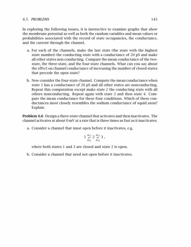
145 6.5. PROBLEMS
In exploring the following issues, it is instructive to examine graphs that show the membrane potential as well as both the random variables and mean values or probabilities associated with the record of state occupancies, the conductance, and the current through the channel.
a. For each of the channels, make the last state (the state with the highest state number) the conducting state with a conductance of 20 pS and make all other states non-conducting. Compare the mean conductance of the two-state, the three-state, and the four-state channels. What can you say about the effect on channel conductance of increasing the number of closed states that precede the open state?
b. Now consider the four-state channel. Compute the mean conductance when state 1 has a conductance of 20 pS and all other states are nonconducting. Repeat this computation except make state 2 the conducting state with all others nonconducting. Repeat again with state 3 and then state 4. Compare the mean conductance for these four conditions. Which of these conductances most closely resembles the sodium conductance of squid axon? Explain.
Problem 6.6 Design a three-state channel that activates and then inactivates. The channel activates at about 0 mV at a rate that is three times as fast as it inactivates.
a. Consider a channel that must open before it inactivates, e.g.
1 τ12�τ21
2τ23 �τ32
3 ,
where both states 1 and 3 are closed and state 2 is open.
b. Consider a channel that need not open before it inactivates.

146 CHAPTER 6. VOLTAGE-GATED ION CHANNELS

Bibliography
Aidley, D. J. (1989). The Physiology of Excitable Cells. Cambridge University Press, Cambridge, Great Britain.
Armstrong, C. M. (1966). Time course of tea+-induced anomalous rectification in squid giant axons. J. Gen. Physiol., 50:491–503.
Armstrong, C. M. and Binstock, L. (1965). Anomalous rectification in the squid giant axon injected with tetraethylammonium chloride. J. Gen. Physiol., 48:859– 872.
Athena (1990a). Computation and Educational Community: A Background Paper. Committee on Academic Computation for the 1990s and Beyond, Massachusetts Institute of Technology.
Athena (1990b). Computing for Education at MIT: Final Report. Committee on Academic Computation for the 1990s and Beyond, Massachusetts Institute of Technology.
Baker, P. F., Hodgkin, A. L., and Shaw, T. I. (1961). Replacement of the protoplasm of a giant nerve fibre with artificial solutions. Nature, 190:885–887.
Balestri, D. (1988). Ivory towers, silicon basements. Infor. Tech. Quaterly, 7:5–17.
Berkenblit, S. I. (1990). Design of a software diffusion simulator and analysis of a problem in two-compartment diffusion. Master’s thesis, Massachusetts Institute of Technology, Cambridge, MA.
Carruthers, A. (1984). Sugar transport in animal cells: The passive hexose transfer system. Prog. Biophys. Mol. Biol., 43:33–69.
Colquhoun, D. and Hawkes, A. G. (1977). Relaxation and fluctuations of membrane currents that flow through drug-operated channels. Proc. R. Soc. London, Ser. B, 199:231–262.
Colquhoun, D. and Hawkes, A. G. (1995a). The principles of the stochastic interpretation of ion-channel mechanisms. In Sakmann, B. and Neher, E., editors, Single-Channel Recording, pages 397–482. Plenum Press, New York, NY.
147

148 BIBLIOGRAPHY
Colquhoun, D. and Hawkes, A. G. (1995b). A Q-matrix cookbook. How to write only one program to calculate the single-channel and macroscopic predictions for any kinetic mechanism. In Sakmann, B. and Neher, E., editors, Single-Channel Recording, pages 589–633. Plenum Press, New York, NY.
Cox, D. R. and Miller, H. D. (1965). The Theory of Stochastic Processes. John Wiley and Sons, New York, NY.
Einstein, A. (1906). Sur theorie der brownschen bewegung. Ann. Physik, 19:371– 381. [For translation see Einstein (1956)].
Einstein, A. (1956). Investigations on the Theory of the Brownian Movement. Dover Publications. R. Furthe and A. D. Cowper, eds. [Translation of original publications].
Fick, A. (1855). On liquid diffusion. Philos. Mag., 10:30–39.
Frankenhaeuser, B. and Hodgkin, A. L. (1957). The action of calcium on the electrical properties of squid axons. J. Physiol., 137:218–244.
Gerald, C. F. and Wheatley, P. O. (1989). Applied Numerical Analysis. Addison-Wesley, Reading, MA.
Hanselman and Littlefield (1996). Mastering MATLAB. Prentice-Hall, Englewood Hills, NJ.
Hille, B. (1992). Ionic Channels of Excitable Membranes. Sinauer Associates Inc., Sunderland, MA.
Hodgkin, A. L. (1964). The Conduction of the Nervous Impulse. Charles C. Thomas, Springfield, IL.
Hodgkin, A. L. and Huxley, A. F. (1952). A quantitative description of membrane current and its application to conduction and excitation in nerve. J. Physiol., 117:500–544.
Hodgkin, A. L. and Katz, B. (1949a). The effect of sodium ions on the electrical activity of the giant axon of the squid. J. Physiol., 108:37–77.
Hodgkin, A. L. and Katz, B. (1949b). The effect of temperature on the electrical activity of the giant axon of the squid. J. Physiol., 109:240–249.
Huxley, A. F. (1959). Ion movements during nerve activity. Ann. N.Y. Acad. Sci., 81:221–246.
Johnston, D. and Wu, S. M. S. (1995). Foundations of Cellular Neurophysiology. MIT Press, Cambridge, MA.
149 BIBLIOGRAPHY
Kandel, E. R., Schwartz, J. H., and Jessell, T. M. (1991). Principles of Neural Science. Elsevier, New York, NY.
Katz, B. (1966). Nerve, Muscle and Synapse. McGraw-Hill Inc., New York, NY.
Keynes, R. D. and Aidley, D. J. (1991). Nerve and Muscle. Cambridge University Press, Cambridge, Great Britain.
Kulik, C. C. and Kulik, J. A. (1986). Effectiveness of computer-based education in colleges. AEDS J., pages 81–108.
Neher, E. and Sakmann, B. (1976). Single-channel currents recorded from membrane of denervated frog muscle fibres. Nature, 260:799–802.
Nicholls, J. G., Martin, A. R., and Wallace, B. G. (1992). From Neuron to Brain: A Cellular and Molecular Approach to the Function of the Nervous System. Sinauer Associates, Sunderland, MA.
Plonsey, R. and Barr, R. C. (1988). Bioelectricity, A Quantitative Approach. Plenum Press, New York, NY.
Press, W. H., Flannery, B. P., Teukolsky, S. A., and Vetterling, W. T. (1986). Numerical Recipes. The Art of Scientific Computing. Cambridge University Press, Cambridge, Great Britain.
Press, W. H., Flannery, B. P., Teukolsky, S. A., and Vetterling, W. T. (1988). Numerical Recipes in C. The Art of Scientific Computing. Cambridge University Press, Cambridge, Massachusetts.
Shah, D. M. (1990). Computer simulation of the random walk model of diffusion. Bachelor’s thesis, Massachusetts Institute of Technology, Cambridge, MA.
Shampine, L. F. and Reichelt, M. W. (1997). The MATLAB ODE suite. SIAM J. Sci. Comput., 18:1–22.
Stein, W. D. (1986). Transport and Diffusion Across Cell Membranes. Academic Press, New York, NY.
Tasaki, I. and Hagiwara, S. (1957). Demonstration of two stable potential states in the squid giant axon under tetraethylammonium chloride. J. Gen. Physiol., 40:859–885.
Weiss, T. F. (1996a). Cellular Biophysics. Volume 1: Transport. MIT Press, Cambridge, MA.
Weiss, T. F. (1996b). Cellular Biophysics. Volume 2: Electrical Properties. MIT Press, Cambridge, MA.

150 BIBLIOGRAPHY
Weiss, T. F., Trevisan, G., Doering, E. B., Shah, D. M., Huang, D., and Berkenblit, S. I. (1992). Software for teaching physiology and biophysics. J. Sci. Ed. Tech., 1:259–274.
Wilson, J. M. and Redish, E. F. (1989). Using computers in teaching physics. Physics Today, pages 34–41.