center for infrastructure engineering...

��

CENTER FOR INFRASTRUCTURE ENGINEERING STUDIES

IN-SITU LOAD TESTI

LEXING

B

Nestor

Paolo

a

Antoni

University TransportaThe University

UTC

R124-1

NG OF BRIDGE A6101

TON, MO

y

e Galati

Casadei

nd

o Nanni

tion Center Program at of Missouri-Rolla

The contents of this report reflect for the facts and the accuracy of disseminated under the sponsorshUniversity Transportation CenterEngineering Studies UTC prograinterest of information exchange.Infrastructure Engineering Studithereof.

Disclaimer

the views of the author(s), who are responsibleinformation presented herein. This document isip of the Department of Transportation,

s Program and the Center for Infrastructure m at the University of Missouri - Rolla, in the The U.S. Government and Center for es assumes no liability for the contents or use

Technical Report Documentation Page

1. Report No.

UTC R124-1 2. Government Accession No. 3. Recipient's Catalog No.

5. Report Date

January 2005

4. Title and Subtitle

In-situ load testing of Bridge A6101 Lexington, MO

6. Performing Organization Code

7. Author/s

Nestore Galati, Paolo Casadei, and Antonio Nanni

8. Performing Organization Report No.

00001104

10. Work Unit No. (TRAIS) 9. Performing Organization Name and Address

Center for Infrastructure Engineering Studies/UTC program University of Missouri - Rolla 223 Engineering Research Lab Rolla, MO 65409

11. Contract or Grant No.

DTRS98-G-0021

13. Type of Report and Period Covered

Final

12. Sponsoring Organization Name and Address

U.S. Department of Transportation Research and Special Programs Administration 400 7th Street, SW Washington, DC 20590-0001

14. Sponsoring Agency Code

15. Supplementary Notes

16. Abstract

The scope of this project is the evaluation of a High Performance Steel (HPS) bridge located in the City of Lexington in Lafeyette County, Mo. The bridge number is A6101 and it is located on Mo. Rt. 224/Mo. Rt.13. To evaluate the load-carrying capacity of the bridge, a nondestructive field test was conducted. The bridge was tested both statically and dynamically using six H20-44 trucks as specified in AASHTO (2002). The dynamic load was applied by moving the trucks at different speeds over the bridge deck.

The bridge deflection under static load was measured using a robotic tacheometry (“total station”) system (RTS) that offers a non-contact deflection measurement technique. RTS has the capability to measure the spatial coordinates of discrete points on a bridge in three dimensions without having to touch the structure. In this project, both RTS and conventional extensometers (LVDTs) were used to measure the bridge deflections. The RTS was used to monitor the deflection of 19 points located on the bridge girders. The LVDTs were primarily used to measure the dynamic deflection of the bridge; they were mounted in correspondence to three prisms monitored by the total station in order to validate the accuracy of the latter during the static test.

17. Key Words

assessment, bridge monitoring, concrete deck, high performance steel, in-situ load test, structural evaluation, thermal effects, total station.

18. Distribution Statement

No restrictions. This document is available to the public through the National Technical Information Service, Springfield, Virginia 22161.

19. Security Classification (of this report)

Unclassified

20. Security Classification (of this page)

Unclassified

21. No. Of Pages

22. Price

Form DOT F 1700.7 (8-72)

RESEARCH INVESTIGATION RI04-006

IN-SITU LOAD TESTING OF BRIDGE A6101

LEXINGTON, MO

PREPARED FOR THE

MISSOURI DEPARTMENT OF TRANSPORTATION

IN COOPERATION WITH THE

UNIVERSITY TRANSPORTATION CENTER

Written By:

Nestore Galati, Research Engineer

Paolo Casadei, PhD Candidate

Antonio Nanni, V. & M. Jones Professor of Civil Engineering

CENTER FOR INFRASTRUCTURE ENGINEERING STUDIES

UNIVERSITY OF MISSOURI – ROLLA

Submitted

January 2005

The opinions, findings and conclusions expressed in this report are those of the principal investigators. They are not necessarily those of the Missouri Department of Transportation, U.S. Department of Transportation, Federal

Highway Administration. This report does not constitute a standard, specification or regulation.

III

IN-SITU LOAD TESTING OF BRIDGE A6102

LEXINGTON, MO

EXECUTIVE SUMMARY

This report presents the evaluation of a High Performance Steel (HPS) bridge through load testing. The bridge is located in the city of Lexington in Lafeyette County, MO. The bridge number is A6101 and it is located on Mo. Rt. 224/Mo. Rt.13. A nondestructive field test was conducted. The bridge was tested both statically and dynamically using six MS18 trucks as specified in AASHTO (2002). The dynamic load was applied by moving the trucks at different speeds on the bridge deck. The bridge deflection under static load was measured using a robotic tacheometry (“total station”) system (RTS), that offers non-contact deflection measurement technique. RTS has the capability to measure the spatial coordinates of discrete points on a bridge in three dimensions without having to touch the structure. In this project, both RTS and conventional extensometers (LVDTs) were used to measure the bridge deflections. The RTS was used to monitor the deflection of 19 points located on the bridge girders. The LVDTs were primarily used to measure the dynamic deflection of the bridge; they were mounted in correspondence to three prisms monitored by the total station in order to validate the accuracy of the latter during the static test. The comparison between theoretical results according to the AASTHO Standard Specifications and experimental data and between static and dynamic loads allowed establishing the safety of the structure. A Finite Element Method (FEM) analysis was undertaken. The numerical model was able to represent the behavior of the bridge and therefore could be used to determine its load rating.

IV

ACKNOWLEDGMENTS

The project was made possible with the financial support received from the Missouri Department of Transportation, UMR - University Transportation Center on Advanced Materials, and the Center for Infrastructure Engineering Studies at the University of Missouri-Rolla. The authors would like to acknowledge John Wenzlick, Research and Development Engineer at MoDOT, for his assistance in different tasks of the project.

V

TABLE OF CONTENTS

TABLE OF CONTENTS.................................................................................................. VI LIST OF FIGURES .........................................................................................................VII LIST OF TABLES............................................................................................................ IX NOTATIONS..................................................................................................................... X 1 INTRODUCTION ...................................................................................................... 1

1.1 Background..........................................................................................................1 1.1.1 Historical Background on High Performance Steel Bridges ...........................1 1.1.2 Live-Load Deflections .....................................................................................2 1.1.3 Diagnostic Load Testing ..................................................................................2

1.2 Bridges Description .............................................................................................3 1.3 Objectives ............................................................................................................5 1.4 Description Measurement Technologies..............................................................5

1.4.1 Total station .....................................................................................................5 1.4.2 Data Acquisition System: Orange Box............................................................7

2 FIELD EVALUATION .............................................................................................. 9 2.1 Bridge Instrumentation ........................................................................................9 2.2 Test Procedure ...................................................................................................10 2.3 Test Results........................................................................................................12

2.3.1 Static Test.......................................................................................................12 2.3.2 Dynamic Test .................................................................................................17

2.4 Discussion of Results.........................................................................................17 2.5 FEM Analysis ....................................................................................................22

3 CONCLUSIONS....................................................................................................... 26 4 REFERENCES ......................................................................................................... 27 APPENDIX I – LOAD TEST STOPS.............................................................................. 29

VI

LIST OF FIGURES

Figure 1 Bridge Details (all dimensions in mm)............................................................................. 3

Figure 2 Framing Plan (all dimensions in mm) ............................................................................. 4

Figure 3 Side View Bridge A6101................................................................................................. 4

Figure 4 Total Station ..................................................................................................................... 6

Figure 5 Data Acquisition System (“Orange Box”) ....................................................................... 7

Figure 6 Target Positions: Plan View (Drawing not in scale) ........................................................ 9

Figure 7 Tower to Mount the LVDTs............................................................................................. 9

Figure 8 MS18 Trucks .................................................................................................................. 10

Figure 9 Transversal Position of the Trucks Stops 1 to 5 ............................................................. 11

Figure 10 Transversal Position of the Trucks Stop 7.................................................................... 11

Figure 11 Trucks Aligned on Stop 2............................................................................................. 11

Figure 12 Longitudinal Deflections Girder 1 Stops 1 to 5............................................................ 12

Figure 13 Transversal Deflections at L/2 from abutment 1 Stops 1 to 6...................................... 13

Figure 14 Longitudinal Deflections Girder 1 Stops 7 and 8......................................................... 14

Figure 15 Transversal Deflections at L/2 from abutment 1 Stops 7 and 8 ................................... 14

Figure 16 LVDTs Readings for Stops 1 to 3 ................................................................................ 15

Figure 17 LVDTs Readings for Stops 6 to 8 ................................................................................ 15

Figure 18 Comparison Between LVDTs and Data from the Total Station (Targets 1, 18 and 19)............................................................................................................................................... 16

Figure 19 Displacement from LVDT 1 at Different Speeds......................................................... 17

Figure 20 Comparison Between AASTHO Provisions and Experimental Results ...................... 18

Figure 21 Comparison between AASTHO Provisions and Corrected Experimental Results ...... 19

Figure 22 Comparison Between AASTHO Provisions and Experimental Results (Transversal Deflections at L/2 from abutment 1, Stops 1 to 5)................................................................ 20

Figure 23 Comparison Between AASTHO Provisions and Corrected Experimental Results (Transversal Deflections at L/2 from abutment 1, Stops 2 to 5)........................................... 21

Figure 24 Finite Element Model of the Bridge............................................................................. 22

Figure 25 Comparison between FEM Model and Experimental Results (Stops 1 to 5)............... 23

Figure 26 Comparison between FEM Model and Corrected Experimental Results (Stops 2 to 5)............................................................................................................................................... 24

Figure 27 Comparison between FEM Model and Experimental Results (Transversal Deflections at L/2 from abutment 1, Stops 1 to 5) ................................................................................... 25

VII

Figure 28 Comparison between FEM Model and Corrected Experimental Results (Transversal Deflections at L/2 from abutment 1, Stops 2 to 5)................................................................ 26

VIII

LIST OF TABLES

Table 2.1 Trucks Used for the Test............................................................................................... 10

IX

NOTATIONS

yf : Steel Yielding Strength

PM : Plastic Moment Capacity

yM : Yield Moment Capacity

1P : Front Load Axle

2P : Rear Load Axle

X

1 INTRODUCTION

1.1 Background

1.1.1 Historical Background on High Performance Steel Bridges Collaboration between government and industry has led to the development of high performance steel (HPS) for bridge applications. HPS offers increased yield strength, enhanced weldability, and improved toughness, and it may lead to lighter and more economical structures. The introduction of High Performance Steel (HPS) with minimum yield strength of 485 MPa (HPS-485W) in 1994 and its utilization in bridge design and construction coincided with various design limitations imposed by AASHTO bridge design specifications. At the time, these limitations reflected the lack of test data to fully comprehend the behavior of bridges constructed using HPS. The code limitations were addressed through multiple research projects funded by the HPS steering committee and the Federal Highway Association (FHWA) IBRC program. As a result, a coordinated national effort was initiated by the steel industry to address these limitations. The effort was coordinated by the American Iron and Steel Institute’s (AISI) steel bridge task force and HPS Design Advisory Group, in close cooperation with the AASHTO T-14 committee (Steel Bridges).

The 1998 version of the AASHTO LRFD Bridge Design Specifications marked the first time where design limitations were imposed (AASHTO 1998). Following is a summary of the various design issues that either had HPS related limitations in the 1998 version of the AASHTO code or were a concern for designers (Azizinamini et al. 2004).

• For continuous plate girders with compact negative sections, the maximum moment capacity was limited to yield moment capacity of the section, My, rather than the plastic moment capacity, Mp, as used for lower grade steels.

• Inelastic methods of analysis and design were not permitted for HPS plate girders with yield strength equal to or exceeding 485 MPa. It should be noted that this also disallows the use of the 10% moment redistribution for girders comprised of compact sections.

• Information to check the ductility of composite plate girders in the positive section, per requirements stated in section 6.10.4.2.2 of the AASHTO LRFD bridge design specification, was incomplete. As a result, one could conclude that HPS could not be used in the positive sections since ductility check provisions were not available.

• In the initial stages of introducing HPS, there was a concern that HPS plates may not be able to develop large tensile strains without fracture. Some of the examples included use of HPS as tension flanges of plate girders in positive sections or use of HPS as tension members in trusses. These concerns were mainly a result of work by McDermott (1969) who conducted tests on A514 690 MPa steel girders. When these girders were loaded in three-point bending, the high strength steel tension flange fractured very shortly after yielding.

• For years, AASHTO codes had limited the shear capacity of the hybrid plate girders to the elastic buckling capacity of the panel. Hybrid girders consist of using higher grades of steel for flanges and lower grades for the web. For instance, using 345 MPa steel for

1

flanges and 250 MPa steel for webs, or using 485 MPa steel for flanges and 345 MPa steels for webs. This limitation was not confined to HPS. It also applied to hybrid girders fabricated with 345 and 250 MPa steels. What made this limitation important was the fact that it has been shown that the best use of HPS in plate girders is in the hybrid form where flanges are constructed using 485 MPa steels and webs are constructed using 345 MPa steels (Horton et al. 2000). Design studies have indicated that for many typical situations hybrid girders will produce the most economical designs (Barker and Schrage 2000; Horton et al. 2000; Clingenpeel and Barth 2003).

• Current specifications place limits on the maximum allowable live load deflections. These requirements have not typically controlled the geometry of sections designed with steel having fy<345 MPa. However, due to the reduced section geometries required when HPS-485W steel is incorporated, these limits may be the controlling limit state for some design situations. Therefore, research has been initiated to investigate the rationale behind the current limits and to assess their influence on the serviceability and economy of HPS bridges.

• In addition to incorporating HPS 70W in traditional I girder configurations, it was felt that innovative concepts capitalizing on both the increased strength and improved toughness of the steel may also produce cost effective structures. Some of the design innovations that have been developed may prove to be beneficial for various steel grades (e.g., Grade 50, HPS 70W, of HPS 100W).

1.1.2 Live-Load Deflections The AASHTO standard specifications (1996) place a limit on the maximum allowable live-load deflection of L/800 for most bridges and L/1000 for bridges subject to pedestrian use. Similar specifications are given in the AASHTO LRFD specifications (1998). It should be noted that the LRFD specifications are specifically written as optional criteria; however, many states Transportation Departments will continue to view them as mandatory requirements (Azizinamini et al. 2004). For traditional steel bridge comprised of steels with fy<345 MPa, these limits have rarely been found to control girder geometries. However, recent studies have shown that for some design situations with HPS 70W, particularly in cases with high span-to-depth ratios, these limits may have a significant influence on the final section requirements (Roeder et al. 2001; Barth et al. 2004; Roeder et al. 2004).

A recent research study focusing on examining the influence of these limits on steel I girder bridge design showed that to date there is not a relationship between either reported bridge damage or objectionable vibration characteristics with a direct check of live load deflections (Roeder et al. 2001; Barth et al. 2004; Roeder et al. 2004).

1.1.3 Diagnostic Load Testing Field testing is an increasingly important topic in the effort to deal with new infrastructures using new technologies as well as deteriorating infrastructure, in particular bridges and pavements. There is a need for accurate and inexpensive methods for diagnostics, verification of load distribution and determination of the actual load carrying capacity.

Recent studies indicate that 40 percent of the national bridges are deficient. The major factors that have contributed to the present situation are: the age, inadequate maintenance, increasing

2

load spectra and environmental contamination. The deficient bridges are posted, repaired or replaced. The disposition of bridges involves clear economical and safety implications. To avoid high costs of replacement or repair, the evaluation must accurately reveal the present load carrying capacity of the structure and predict loads and any further changes in the capacity (deterioration) in the applicable time span (Deza, 2004).

Frequently, diagnostic load tests reveal strength and serviceability characteristics that exceed the predicted codified parameters. Usually, codified parameters are very conservative in predicting lateral load distribution characteristics and the influence of other structural attributes. As a result, the predicted rating factors are typically conservative (Chajes et al. 1997).

1.2 Bridges Description The bridge under investigation was just opened to traffic at the time of this load test. It was designed using a standard MS18 truck with military 106 kN tandem axle. The bridge is built with two continuous 42 m long spans with central support consisting of a reinforced concrete (RC) bent supported by three RC circular piers. The bridge is 12.82 m wide and carries two lanes of traffic. The superstructure consists of two continuous spans having a skew angle of 11o 58` 4``. The cross section consists of five composite, equally spaced, HPS girders supporting a RC deck (See Figure 1).

12820

950 2730 2730 2730 2730 950

220

a) Cross Section of the Bridge (Drawing not to scale)

CL Bent 2

Plate 20x420

Plate 20x320

12 Web Plate

Plate 32x520

Plate 32x520 HPS 485W

Plate 32x520

Plate 32x520

Plate 32x520

Plate 20x320

Plate 20x320

Plate 32x520 HPS 485WCL LC Abutment 3

8960 5300 7500 7500 293605300

42160 42160

Plate 20x420

15000 5400

12 Web Plate

Abutment 1

a) Side View of the Girders (Drawing not to scale, Steel Grade 345 W unless specified)

Figure 1 Bridge Details (all dimensions in mm)

3

Layout and typical diaphragms are detailed in Figure 2.

6581 28000 7419 6581 28000 7419

7419 4 Spa. @ 7000 = 28000 6581 7419 4 Spa. @ 7000 = 28000 6581

5 Sp

a. @

273

0

1092

0

Abutment 3CLLC Abutment 1

Bent 2CL

a) Framing Plan (all dimensions in mm)

102 x 102 x 7.9

102 x 102 x 7.9

10 mm PL 10 mm PL

76 x 76 x 7.9

b) Typical Diaphragm (Drawing not in scale, Steel Grade 345 W unless specified)

Figure 2 Framing Plan (all dimensions in mm)

The bridge overpasses an under-construction highway: this condition simplified the load testing procedure but it was not essential to it. A photograph of the bridge structure is shown in Figure 3.

Figure 3 Side View Bridge A6101

4

1.3 Objectives The scope of this project is the evaluation of a High Performance Steel (HPS) bridge located in the City of Lexington in Lafeyette County, MO. The bridge number is A6101 and it is located on Mo. Rt. 224/Mo. Rt.13.

1.4 Methodology To evaluate the load-carrying capacity of the bridge, a nondestructive field test was conducted. Experimental load testing on a bridge can be categorized as either a diagnostic or proof test. In a diagnostic test, a predetermined load, typically near the bridge's rated capacity, is placed at several different locations along the bridge and the bridge response is measured. The measured response is then used to develop a numerical model of the bridge. The bridge model can then be used to estimate the maximum allowable load. In a proof test, incremental loads are applied to the bridge until either a target load is reached or a predetermined limited state is exceeded. Using the maximum load reached, the capacity of the bridge can be determined. While diagnostic tests provide only an estimate of a bridge's capacity, they have several practical advantages including a lower cost, a shorter testing time, and less disruption to traffic. Because of these advantages, diagnostic testing was used in this case.

The bridge was tested both statically and dynamically using six MS18 trucks as specified in AASHTO (2002). The dynamic load was applied by moving the trucks at different speeds on the bridge deck. The comparison between theoretical and experimental results and between static and dynamic loads allowed determining the safety of the structure.

A major difficulty in the testing and evaluation of bridges in the field is the measurement of vertical deflections. The use of instruments such as mechanical dial gauges, linear potentiometers, linear variable differential transducers (LVDTs), and other similar types of deflection transducers is usually not feasible, because a fixed base is needed from which relative displacements are measured. This often requires access under the bridge to erect a temporary support to mount the instrument or for running a wire from the instrument to the ground. These difficulties can be eliminated using robotic tacheometry (“total station”) systems (RTS), that offer a noncontact deflection measurement technique. RTS has the capability to measure the spatial coordinates of discrete points on a bridge in three dimensions without having to touch the structure.

In this project, both RTS and LVDTs were used to measure the bridge deflections. The RTS was used to monitor the deflection of 19 points located on the bridge girders. The LVDTs were primarily used to measure the dynamic deflection of the bridge; they were mounted in correspondence to three prisms monitored by the total station in order to determine the accuracy of the latter during the static test.

1.5 Description Measurement Technologies

1.5.1 Total station The Total Station used in this project is a Leica TCA2003 (www.leica-geosystems.com) as shown in Figure 4. The instrument sends a laser ray to reflecting prisms mounted on the structure to be monitored, and, by triangulation with fixed reference points placed outside the structure, it can determine how much the element has moved in a three-dimensional array with an accuracy

5

of 0.5 in (12.7 mm) on angular measurements and 1mm+1ppm on distance measurements, in average atmospheric conditions.

Figure 4 Total Station

Total stations have been used to measure the movement of structures and natural processes with good results (Hill and Sippel 2002; Kuhlmann and Glaser 2002). Leica Geosystems quote accuracies of better than 1mm for their bridge and tunnel surveys. They use a remote system that logs measurements 6 times daily via a modem, with measurements still possible at peak times. Kuhlmann and Glaser (2002) used a reflectorless total station to monitor the long term deformation of bridges. Measurements were taken of the whole bridge every six years and statistical tests were used to confirm if the points had moved. Hill and Sippel (2002) used a total station and other sensors to measure the deformation of the land in a landslide region. Merkle (2004) used the total station as part of a 5-year monitoring program for the in-situ load testing prior to and after the strengthening of five existing concrete bridges, geographically spread over three Missouri Department of Transportation (MODOT) districts. The five bridges were strengthened using five different Fiber Reinforced Polymer (FRP) technologies as part of a joint MODOT – University of Missouri-Rolla (UMR) initiative (Lynch, 2004).

There are advantages and disadvantages of using a total station for dynamic deformation monitoring. The advantages include the high accuracy as quoted above, the automatic target recognition which provides precise target pointing (Hill and Sippel 2002) and the possibility of measuring indoors and in urban canyons (Radovanovic and Teskey 2001). The disadvantages include the low sampling rate (Meng 2002), problems with measurement in adverse weather conditions (Hill and Sippel 2002) and the fact that a clear line of sight is needed between the total station and the prism.

Radovanovic and Teskey (2001) conducted experiments to compare the performance of a robotic total station with GPS. This experiment was conducted because GPS is not an option in many application areas such as indoors. Total stations are now capable of automatic target recognition and they can track a prism taking automatic measurements of angles and distances once lock has been established manually. It was found that the total station performed better than GPS in a stop and go situation, where measurements were taken of a moving object only when it was stationary. In a completely kinematic situation, GPS performed the best. It was found that there were two main problems with the total station in kinematic mode. These were a low EDM

6

accuracy caused by a ranging error that was linearly dependent upon the line of sight velocity; and an uneven sampling rate over time worsened by no time tagging.

For this experimental program, LVDTs were chosen to be used for the dynamic characterization of the bridge, instead of the total station. In order to read the data from the LVDTs, an in-house made data acquisition system was used. The system is able to read data up to 100 Hz and it was named “Orange Box”.

1.5.2 Data Acquisition System A portable data acquisition unit, suitable for use in field testing of structures, has been custom-manufactured at UMR. It is capable of recording 32 high-level channels of data, 16 strain channels, and 32 thermocouple channels, as well as interfacing a Leica Total Station surveying instrument (See Figure 5).

Figure 5 Data Acquisition System (“Orange Box”)

The high-level channels may receive DC LVDT's, string transducers, linear potentiometers, or any other +/- 10 Volt DC signal. The strain channels can be used to monitor and record strain gage signals, load cells, strain-based displacement transducers, or any strain based signal. The 32 thermocouple channels are configured for type T thermocouples.

The unit consists of a shock-mounted transport box, with removable front and rear covers. Removal of the front cover exposes the computer keyboard and LED display, as well as the front panel of the data acquisition equipment. Removal of the back panel exposes the connector bay, where cables from all the transducers terminate.

The data acquisition system is comprised of National Instruments equipment, listed below:

1. A PXI-1010 SCXI combination unit, which houses the industrial-grade 2.2 GHz Pentium 4 computer, floppy drive, and CDR/W module;

2. A PXI-6030E Analog to Digital converter module for doing the A/D conversion in the system;

3. A pair of SCXI-1520 modules to interface strain based sensors;

7

4. A SCXI-1102B module for multiplexing high-level sensors;

5. A SCXI-1102B module for multiplexing thermocouple sensors;

6. I/O devices in order to connect additional peripherals and other data acquisition systems such as a Leica Total Station surveying instrument.

The data acquisition system is controlled by a custom made LabVIEW program installed on a built-in computer, which allows control of data rate, sensor selection and calibration, and display of the data. The integration of data from sensors and the Total Station yields a data acquisition system which provides better answers in the field.

8

2 FIELD EVALUATION

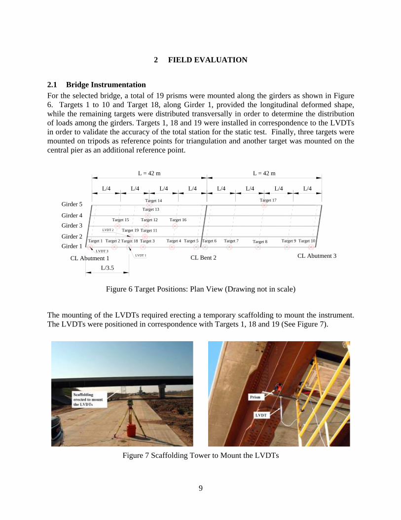
2.1 Bridge Instrumentation For the selected bridge, a total of 19 prisms were mounted along the girders as shown in Figure 6. Targets 1 to 10 and Target 18, along Girder 1, provided the longitudinal deformed shape, while the remaining targets were distributed transversally in order to determine the distribution of loads among the girders. Targets 1, 18 and 19 were installed in correspondence to the LVDTs in order to validate the accuracy of the total station for the static test. Finally, three targets were mounted on tripods as reference points for triangulation and another target was mounted on the central pier as an additional reference point.

L = 42 m L = 42 m

L/4L/4L/4L/4L/4L/4L/4L/4

Target 14

Target 6Target 5Target 1 Target 10

Target 17

Target 2 Target 3 Target 4 Target 7 Target 8 Target 9Girder 1Girder 2

Girder 3Girder 4

Girder 5

CL Abutment 3CL Bent 2CL Abutment 1

Target 11

Target 12

Target 13

Target 15 Target 16

Target 18

Target 19

L/3.5

LVDT 1

LVDT 2

LVDT 3

Figure 6 Target Positions: Plan View (Drawing not in scale)

The mounting of the LVDTs required erecting a temporary scaffolding to mount the instrument. The LVDTs were positioned in correspondence with Targets 1, 18 and 19 (See Figure 7).

Figure 7 Scaffolding Tower to Mount the LVDTs

9

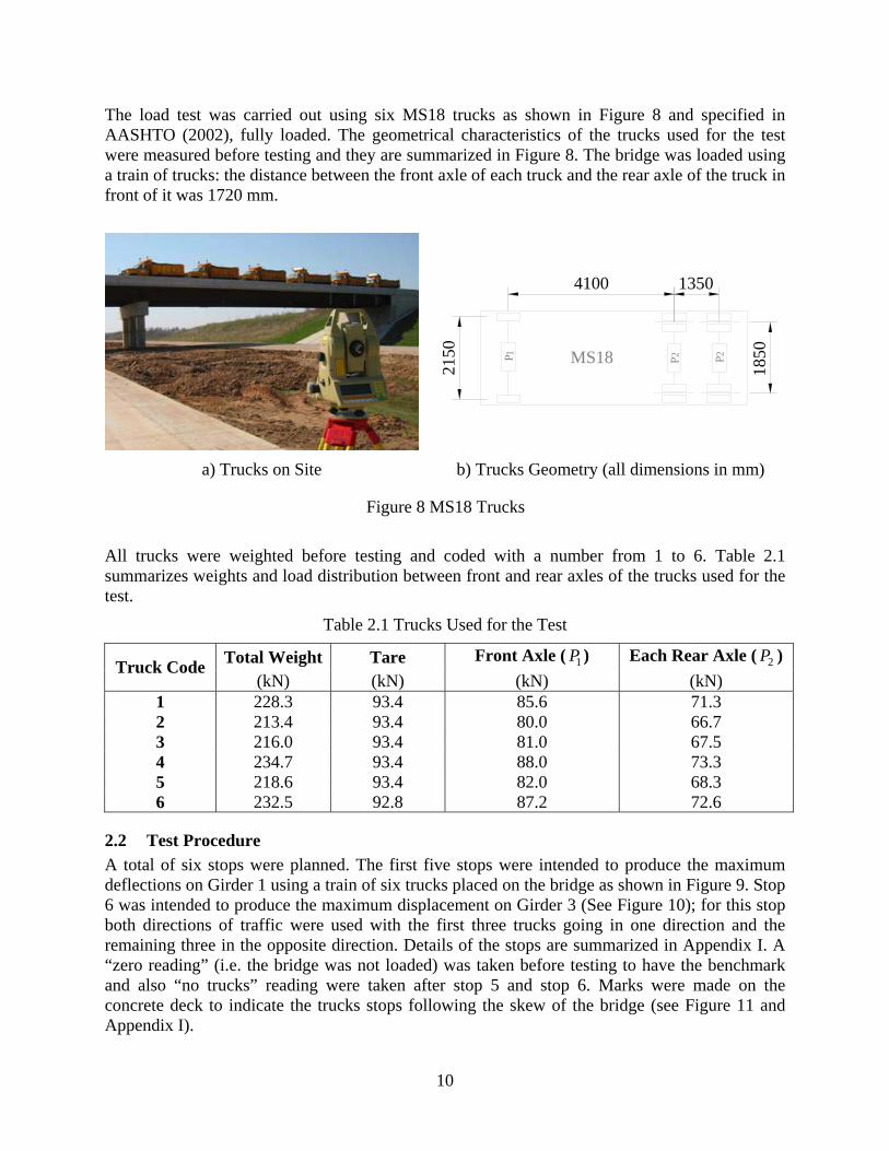
The load test was carried out using six MS18 trucks as shown in Figure 8 and specified in AASHTO (2002), fully loaded. The geometrical characteristics of the trucks used for the test were measured before testing and they are summarized in Figure 8. The bridge was loaded using a train of trucks: the distance between the front axle of each truck and the rear axle of the truck in front of it was 1720 mm.

MS18 PP 221P

4100 1350

1850

2150

a) Trucks on Site b) Trucks Geometry (all dimensions in mm)

Figure 8 MS18 Trucks

All trucks were weighted before testing and coded with a number from 1 to 6. Table 2.1 summarizes weights and load distribution between front and rear axles of the trucks used for the test.

Table 2.1 Trucks Used for the Test

Total Weight Tare Front Axle ( ) 1P Each Rear Axle ( ) 2PTruck Code

(kN) (kN) (kN) (kN) 1 228.3 93.4 85.6 71.3 2 213.4 93.4 80.0 66.7 3 216.0 93.4 81.0 67.5 4 234.7 93.4 88.0 73.3 5 218.6 93.4 82.0 68.3 6 232.5 92.8 87.2 72.6

2.2 Test Procedure A total of six stops were planned. The first five stops were intended to produce the maximum deflections on Girder 1 using a train of six trucks placed on the bridge as shown in Figure 9. Stop 6 was intended to produce the maximum displacement on Girder 3 (See Figure 10); for this stop both directions of traffic were used with the first three trucks going in one direction and the remaining three in the opposite direction. Details of the stops are summarized in Appendix I. A “zero reading” (i.e. the bridge was not loaded) was taken before testing to have the benchmark and also “no trucks” reading were taken after stop 5 and stop 6. Marks were made on the concrete deck to indicate the trucks stops following the skew of the bridge (see Figure 11 and Appendix I).

10

Girder 1

950 1850

Figure 9 Transverse Position of the Trucks for Stops 1 to 5

3680 1850

Girder 1 Girder 2 Girder 4Girder 3 Girder 5

36801850

Figure 10 Transverse Position of the Trucks for Stop 7

Figure 11 Trucks Aligned on Stop 2

Once the total station was leveled and acclimatized, initial readings were taken for each prism. Then, the trucks drove to the first stop. At each stop, before acquiring data, ten minutes lapsed to allow for potential settlements. To assure stable measurements, three readings were taken for

11

each target in order to average out possible errors. Once the reading was terminated, the trucks moved to the next stop and the same procedure was repeated. The Data Acquisition System was recording continuously at a frequency of 1 Hz.

A dynamic test was conducted in order to determine the impact factor by moving the train of trucks on the same line for stops 1 to 6 at speeds equal to 5, 10, 20 and 30 MPH (2.2, 4.5, 8.9 and 13.4 m/s). Since it was very difficult to keep the train of six trucks together, the test was repeated using only trucks 1, 2 and 3 with speeds 1, 5 and 10 MPH (0.4, 2.2 and 4.5 m/s); it was decided not to use higher speeds because the significant amount of dust produced during the test created an unsafe environment for the drivers.

The dynamic test was performed acquiring the data only from the LVDTs at a frequency of 50 Hz.

2.3 Test Results

2.3.1 Static Test The vertical deflections resulting from the load testing are given in below. Figure 12 shows the deflection of Girder 1 corresponding to the first five stops. The additional reading indicated as “NO TRUCKS” intended to determine whether the bridge presented permanent deformations after the first five stops. A preliminary examination of the data indicates that the readings are accurate. The consistency of the readings from stop to stop and from pass to pass lends credence to their validity. The curves also exhibit, in general, a smooth transition from point to point.

-60

-50

-40

-30

-20

-10

0

10

20

30

40

0 10.54 21.08 31.62 42.16 52.7 63.24 73.78 84.32z (m)

Dis

plac

emen

t (m

m)

STOP 1 STOP 2STOP 3 STOP 4STOP 5 NO TRUCKS

z

Trucks DirectionSPAN 1 SPAN 2

z

Trucks DirectionSPAN 1 SPAN 2

Figure 12 Longitudinal Deflections Girder 1 Stops 1 to 5

12

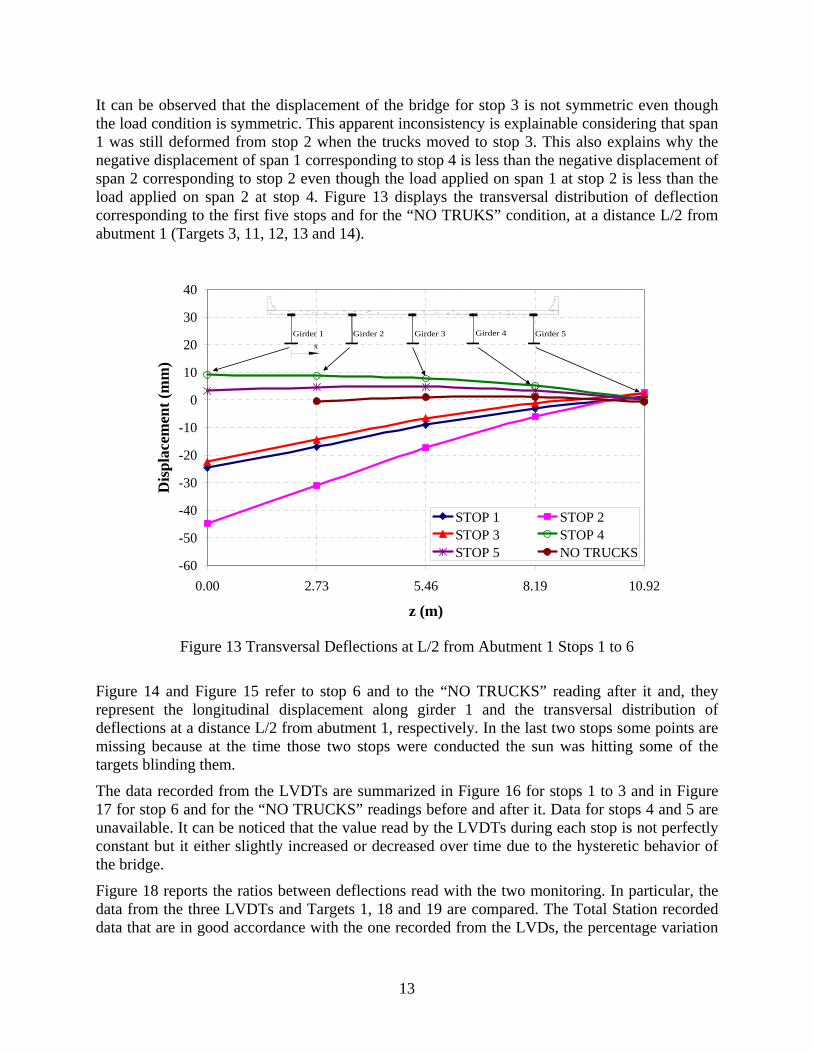
It can be observed that the displacement of the bridge for stop 3 is not symmetric even though the load condition is symmetric. This apparent inconsistency is explainable considering that span 1 was still deformed from stop 2 when the trucks moved to stop 3. This also explains why the negative displacement of span 1 corresponding to stop 4 is less than the negative displacement of span 2 corresponding to stop 2 even though the load applied on span 1 at stop 2 is less than the load applied on span 2 at stop 4. Figure 13 displays the transversal distribution of deflection corresponding to the first five stops and for the “NO TRUKS” condition, at a distance L/2 from abutment 1 (Targets 3, 11, 12, 13 and 14).

-60

-50

-40

-30

-20

-10

0

10

20

30

40

0.00 2.73 5.46 8.19 10.92

z (m)

Dis

plac

emen

t (m

m)

STOP 1 STOP 2STOP 3 STOP 4STOP 5 NO TRUCKS

xGirder 5Girder 3 Girder 4Girder 2Girder 1

Figure 13 Transversal Deflections at L/2 from Abutment 1 Stops 1 to 6

Figure 14 and Figure 15 refer to stop 6 and to the “NO TRUCKS” reading after it and, they represent the longitudinal displacement along girder 1 and the transversal distribution of deflections at a distance L/2 from abutment 1, respectively. In the last two stops some points are missing because at the time those two stops were conducted the sun was hitting some of the targets blinding them.

The data recorded from the LVDTs are summarized in Figure 16 for stops 1 to 3 and in Figure 17 for stop 6 and for the “NO TRUCKS” readings before and after it. Data for stops 4 and 5 are unavailable. It can be noticed that the value read by the LVDTs during each stop is not perfectly constant but it either slightly increased or decreased over time due to the hysteretic behavior of the bridge.

Figure 18 reports the ratios between deflections read with the two monitoring. In particular, the data from the three LVDTs and Targets 1, 18 and 19 are compared. The Total Station recorded data that are in good accordance with the one recorded from the LVDs, the percentage variation

13

of the total station with respect to the LVDTs readings was ranging 0.11% to 9.7% (See Figure 19), providing the necessary confidence in the sensing methods.

-60

-50

-40

-30

-20

-10

0

10

20

30

40

0 10.54 21.08 31.62 42.16 52.7 63.24 73.78 84.32

z (m)

Dis

plac

emen

t (m

m)

STOP 6 NO TRUCKS

z

SPAN 1SPAN 2

z

SPAN 1SPAN 2

Figure 14 Longitudinal Deflections Girder 1 Stops 7 and 8

-60

-50

-40

-30

-20

-10

0

10

20

30

40

0.00 2.73 5.46 8.19 10.92

z (m)

Dis

plac

emen

t (m

m)

STOP 6 NO TRUCKS


Figure 15 Transversal Deflections at L/2 from Abutment 1 Stops 7 and 8

14

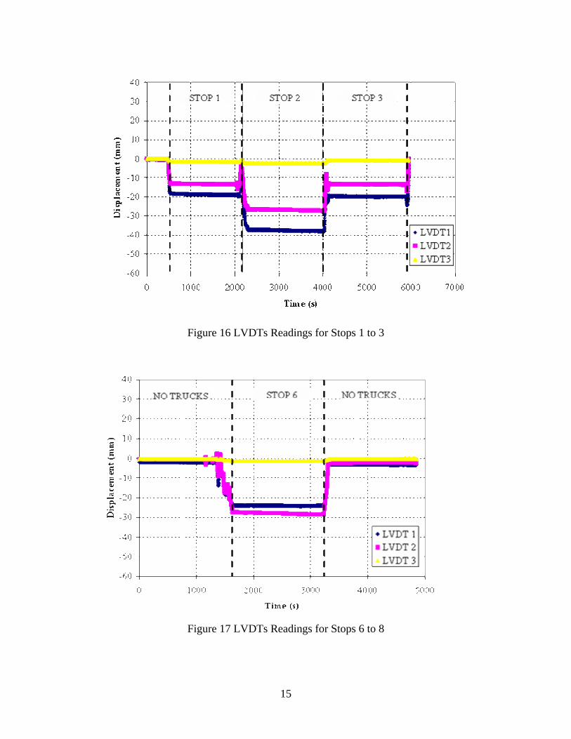
Figure 16 LVDTs Readings for Stops 1 to 3

Figure 17 LVDTs Readings for Stops 6 to 8

15

0.8

0.85

0.9

0.95

1

1.05

1.1

1.15

1.2

1 2 3 4 5 6 7Stops

Dis

plac

emen

t TS

/ Dis

plac

emen

t LV

DT

LVDT 1 / Target 18LVDT 2 / Target 19LVDT 3 / Target 1

No Trucks No Trucks6

Figure 18 Comparison Between LVDTs and Data from the Total Station (Targets 1, 18 and 19)

0

1

2

3

4

5

6

7

8

9

10

1 2 3 4 5 6 7Stops

Perc

enta

ge V

aria

tion

(%)

LVDT 1 / Target 18LVDT 2 / Target 19LVDT 3 / Target 1

No Trucks No Trucks6

Figure 19 Percentage Variation between Total Station and LVDTs readings

16

2.3.2 Dynamic Test The impact factor for the live load was examined by moving the train of six trucks on the path as for stops 1 to 6 at different speeds: 5, 10, 20, 35 and 45 MPH (2.2, 4.5, 8.9, 15.6 and 20.1 m/s). The live load impact factor was computed as the maximum between the ratios of the deflection obtained at a certain speed to the deflection obtained from stops 1 to 6. As an example, Figure 20 shows the deflection measured by LVDT 1 as a function of time for different speeds. From the picture it is possible to observe a decrement of the maximum displacement while increasing the speed of the trucks. This may be partially due to the fact that by increasing the speed, the time of application of the load on the bridge is also reduced and therefore, due to its hysteretic behavior, the corresponding deflections. In addition, at higher speeds, it is difficult for the truck drivers to keep the train of trucks together and this explains the double peak observed at 30 MPH (13.5 m/s).

Considering the train of six trucks the impact factor was found to be -0.18. Such number was determined as the average between the two values for girders 1 and 2. Compared to the computed AASHTO live load impact factor for this bridge, which is 0.30, the AASHTO guidelines appear to be conservative.

Figure 20 Displacement from LVDT 1 at Different Speeds

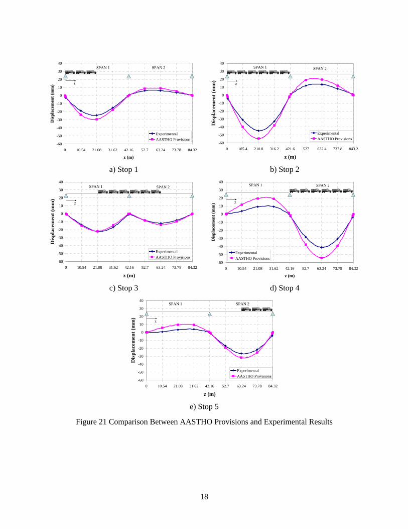
2.4 Discussion of Results The experimental results were compared with the AASHTO LRFD Bridge Design Specifications (AASHTO 1998) section 4.6.2.6. Figure 21 shows a comparison between the deflections of girder 1 computed according to the AASTHO provisions and the experimental results for stops 1 to 5.

The data reported in Figure 21 do not take in account the residual deformation of the bridge after each stop. Figure 22 reports a comparison between the theoretical results calculated according to AASTHO and experimental results corrected to account the residual deformation from the previous stops. This information was obtained for one point from LVDT1 while for the other points it was computed as proportional to the deflection from the previous stops.

17

-60

-50

-40

-30

-20

-10

0

10

20

30

40

0 10.54 21.08 31.62 42.16 52.7 63.24 73.78 84.32

z (m)

Dis

plac

emen

t (m

m)

ExperimentalAASTHO Provisions

z

SPAN 1 SPAN 2

-60

-50

-40

-30

-20

-10

0

10

20

30

40

0 105.4 210.8 316.2 421.6 527 632.4 737.8 843.2

z (m)

Dis

plac

emen

t (m

m)


z

SPAN 1 SPAN 2

a) Stop 1 b) Stop 2

-60

-50

-40

-30

-20

-10

0

10

20

30

40

0 10.54 21.08 31.62 42.16 52.7 63.24 73.78 84.32

z (m)

Dis

plac

emen

t (m

m)


z

SPAN 1 SPAN 2

-60

-50

-40

-30

-20

-10

0

10

20

30

40

0 10.54 21.08 31.62 42.16 52.7 63.24 73.78 84.32

z (m)

Dis

plac

emen

t (m

m)


z

SPAN 1 SPAN 2

c) Stop 3 d) Stop 4

-60

-50

-40

-30

-20

-10

0

10

20

30

40

0 10.54 21.08 31.62 42.16 52.7 63.24 73.78 84.32

z (m)

Dis

plac

emen

t (m

m)


z

SPAN 1 SPAN 2

e) Stop 5

Figure 21 Comparison Between AASTHO Provisions and Experimental Results

18

-60

-50

-40

-30

-20

-10

0

10

20

30

40

0 10.54 21.08 31.62 42.16 52.7 63.24 73.78 84.32

z (m)

Dis

plac

emen

t (m

m)

Experimental CorrectedAASTHO Provisions

z

SPAN 1 SPAN 2

-60

-50

-40

-30

-20

-10

0

10

20

30

40

0 10.54 21.08 31.62 42.16 52.7 63.24 73.78 84.32

z (m)

Dis

plac

emen

t (m

m)


z

SPAN 1 SPAN 2

a) Stop 2 b) Stop 3

-60

-50

-40

-30

-20

-10

0

10

20

30

40

0 10.54 21.08 31.62 42.16 52.7 63.24 73.78 84.32

z (m)

Dis

plac

emen

t (m

m)


z

SPAN 1 SPAN 2

-60

-50

-40

-30

-20

-10

0

10

20

30

40

0 10.54 21.08 31.62 42.16 52.7 63.24 73.78 84.32

z (mm)

Dis

plac

emen

t (m

m)


z

SPAN 1 SPAN 2

c) Stop 4 d) Stop 5

Figure 22 Comparison between AASTHO Provisions and Corrected Experimental Results

From the graphs in Figure 21 and Figure 22 it can be observed that the experimental results are always smaller than the AASTHO guidelines demonstrating in this way the safety of the structure.

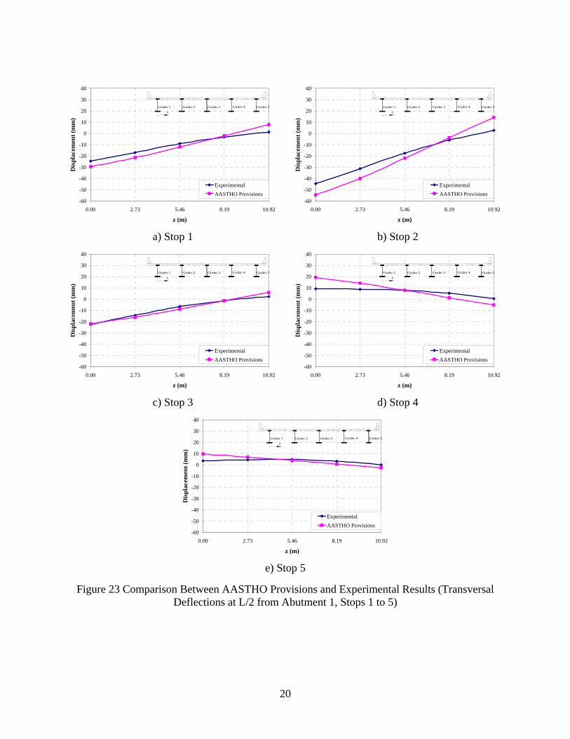
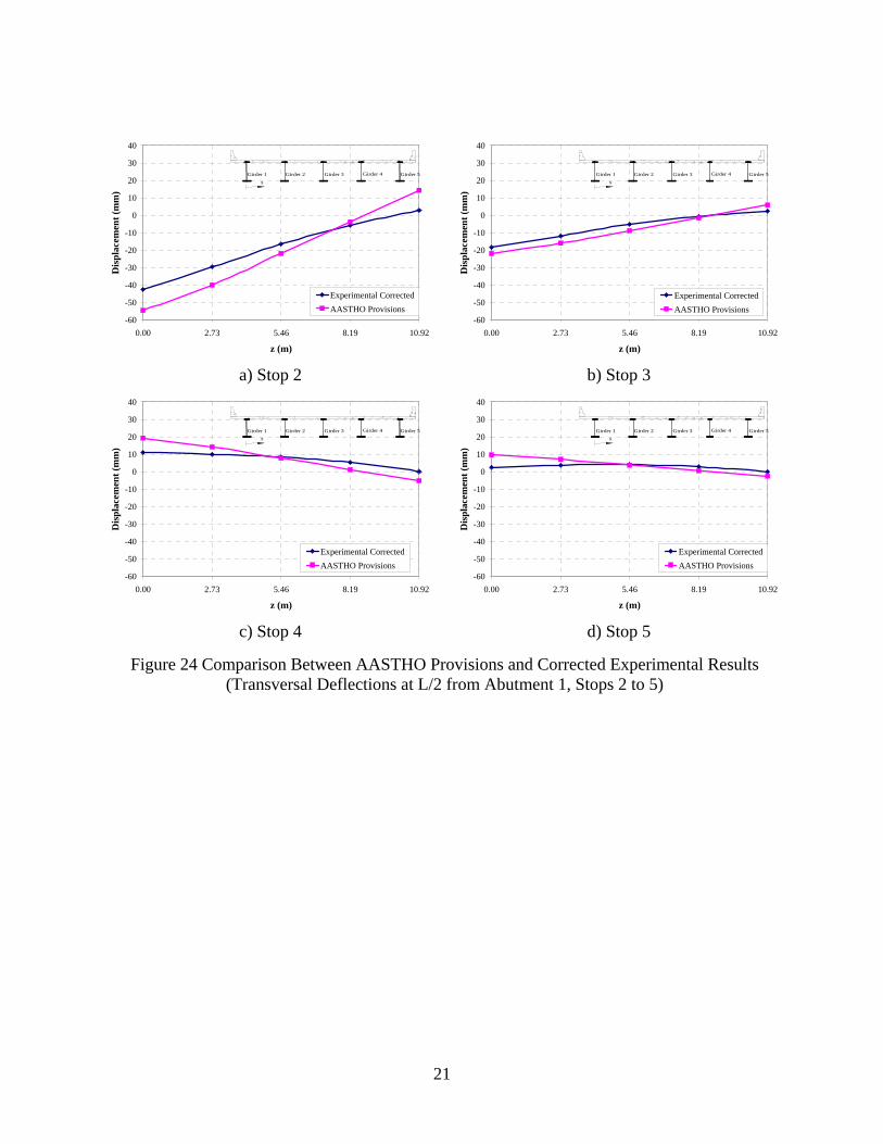
The transversal distribution of deflection at a distance L/2 from abutment 1 is presented in Figure 23 and Figure 24 for uncorrected and corrected results, respectively. The transversal distribution of deflection computed according to the AASTHO guidelines does not accurately describe the actual distribution on the bridge. This is because no composite action between girders and deck is considered in the AASTHO approach, yielding, on the other hand, to a safe design approach.

19

-60

-50

-40

-30

-20

-10

0

10

20

30

40

0.00 2.73 5.46 8.19 10.92

z (m)

Dis

plac

emen

t (m

m)



-60

-50

-40

-30

-20

-10

0

10

20

30

40

0.00 2.73 5.46 8.19 10.92

z (m)

Dis

plac

emen

t (m

m)



a) Stop 1 b) Stop 2

-60

-50

-40

-30

-20

-10

0

10

20

30

40

0.00 2.73 5.46 8.19 10.92

z (m)

Dis

plac

emen

t (m

m)



-60

-50

-40

-30

-20

-10

0

10

20

30

40

0.00 2.73 5.46 8.19 10.92

z (m)

Dis

plac

emen

t (m

m)



c) Stop 3 d) Stop 4

-60

-50

-40

-30

-20

-10

0

10

20

30

40

0.00 2.73 5.46 8.19 10.92

z (m)

Dis

plac

emen

t (m

m)



e) Stop 5

Figure 23 Comparison Between AASTHO Provisions and Experimental Results (Transversal Deflections at L/2 from Abutment 1, Stops 1 to 5)

20

-60

-50

-40

-30

-20

-10

0

10

20

30

40

0.00 2.73 5.46 8.19 10.92

z (m)

Dis

plac

emen

t (m

m)



-60

-50

-40

-30

-20

-10

0

10

20

30

40

0.00 2.73 5.46 8.19 10.92

z (m)

Dis

plac

emen

t (m

m)



a) Stop 2 b) Stop 3

-60

-50

-40

-30

-20

-10

0

10

20

30

40

0.00 2.73 5.46 8.19 10.92

z (m)

Dis

plac

emen

t (m

m)



-60

-50

-40

-30

-20

-10

0

10

20

30

40

0.00 2.73 5.46 8.19 10.92

z (m)

Dis

plac

emen

t (m

m)



c) Stop 4 d) Stop 5

Figure 24 Comparison Between AASTHO Provisions and Corrected Experimental Results (Transversal Deflections at L/2 from Abutment 1, Stops 2 to 5)

21

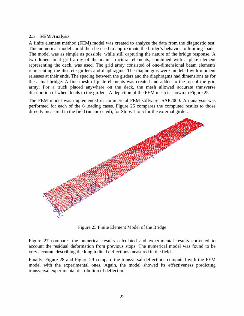
2.5 FEM Analysis A finite element method (FEM) model was created to analyze the data from the diagnostic test. This numerical model could then be used to approximate the bridge's behavior to limiting loads. The model was as simple as possible, while still capturing the nature of the bridge response. A two-dimensional grid array of the main structural elements, combined with a plate element representing the deck, was used. The grid array consisted of one-dimensional beam elements representing the discrete girders and diaphragms. The diaphragms were modeled with moment releases at their ends. The spacing between the girders and the diaphragms had dimensions as for the actual bridge. A fine mesh of plate elements was created and added to the top of the grid array. For a truck placed anywhere on the deck, the mesh allowed accurate transverse distribution of wheel loads to the girders. A depiction of the FEM mesh is shown in Figure 25.

The FEM model was implemented in commercial FEM software: SAP2000. An analysis was performed for each of the 6 loading cases. Figure 26 compares the computed results to those directly measured in the field (uncorrected), for Stops 1 to 5 for the external girder.

Figure 25 Finite Element Model of the Bridge

Figure 27 compares the numerical results calculated and experimental results corrected to account the residual deformation from previous stops. The numerical model was found to be very accurate describing the longitudinal deflections measured in the field.

Finally, Figure 28 and Figure 29 compare the transversal deflections computed with the FEM model with the experimental ones. Again, the model showed its effectiveness predicting transversal experimental distribution of deflections.

22

-60

-50

-40

-30

-20

-10

0

10

20

30

40

0 10.54 21.08 31.62 42.16 52.7 63.24 73.78 84.32

z (m)

Dis

plac

emen

t (m

m)

ExperimentalFEM Analysis

z

SPAN 1 SPAN 2

-60

-50

-40

-30

-20

-10

0

10

20

30

40

0 105.4 210.8 316.2 421.6 527 632.4 737.8 843.2

z (m)

Dis

plac

emen

t (m

m)


z

SPAN 1 SPAN 2

a) Stop 1 b) Stop 2

-60

-50

-40

-30

-20

-10

0

10

20

30

40

0 10.54 21.08 31.62 42.16 52.7 63.24 73.78 84.32

z (m)

Dis

plac

emen

t (m

m)


z

SPAN 1 SPAN 2

-60

-50

-40

-30

-20

-10

0

10

20

30

40

0 10.54 21.08 31.62 42.16 52.7 63.24 73.78 84.32

z (m)

Dis

plac

emen

t (m

m)


z

SPAN 1 SPAN 2

c) Stop 3 d) Stop 4

-60

-50

-40

-30

-20

-10

0

10

20

30

40

0 10.54 21.08 31.62 42.16 52.7 63.24 73.78 84.32

z (m)

Dis

plac

emen

t (m

m)


z

SPAN 1 SPAN 2

e) Stop 5

Figure 26 Comparison between FEM Model and Experimental Results (Stops 1 to 5)

23

-60

-50

-40

-30

-20

-10

0

10

20

30

40

0 105.4 210.8 316.2 421.6 527 632.4 737.8 843.2

z (m)

Dis

plac

emen

t (m

m)

Experimental CorrectedFEM Analysis

z

SPAN 1 SPAN 2

-60

-50

-40

-30

-20

-10

0

10

20

30

40

0 10.54 21.08 31.62 42.16 52.7 63.24 73.78 84.32

z (m)

Dis

plac

emen

t (m

m)


z

SPAN 1 SPAN 2

a) Stop 2 b) Stop 3

-60

-50

-40

-30

-20

-10

0

10

20

30

40

0 10.54 21.08 31.62 42.16 52.7 63.24 73.78 84.32

z (m)

Dis

plac

emen

t (m

m)


z

SPAN 1 SPAN 2

-60

-50

-40

-30

-20

-10

0

10

20

30

40

0 10.54 21.08 31.62 42.16 52.7 63.24 73.78 84.32

z (m)

Dis

plac

emen

t (m

m)


z

SPAN 1 SPAN 2

c) Stop 4 d) Stop 5

Figure 27 Comparison between FEM Model and Corrected Experimental Results (Stops 2 to 5)

24

-60

-50

-40

-30

-20

-10

0

10

20

30

40

0.00 2.73 5.46 8.19 10.92

z (m)

Dis

plac

emen

t (m

m)



-60

-50

-40

-30

-20

-10

0

10

20

30

40

0.00 2.73 5.46 8.19 10.92

z (m)

Dis

plac

emen

t (m

m)



a) Stop 1 b) Stop 2

-60

-50

-40

-30

-20

-10

0

10

20

30

40

0.00 2.73 5.46 8.19 10.92

z (m)

Dis

plac

emen

t (m

m)



-60

-50

-40

-30

-20

-10

0

10

20

30

40

0.00 2.73 5.46 8.19 10.92

z (m)

Dis

plac

emen

t (m

m)



c) Stop 3 d) Stop 4

-60

-50

-40

-30

-20

-10

0

10

20

30

40

0.00 2.73 5.46 8.19 10.92

z (m)

Dis

plac

emen

t (m

m)



e) Stop 5

Figure 28 Comparison between FEM Model and Experimental Results (Transversal Deflections at L/2 from Abutment 1, Stops 1 to 5)

25

-60

-50

-40

-30

-20

-10

0

10

20

30

40

0.00 2.73 5.46 8.19 10.92

z (m)

Dis

plac

emen

t (m

m)

Experimental CorrectFEM Analysis


-60

-50

-40

-30

-20

-10

0

10

20

30

40

0.00 2.73 5.46 8.19 10.92

z (m)

Dis

plac

emen

t (m

m)



a) Stop 2 b) Stop 3

-60

-50

-40

-30

-20

-10

0

10

20

30

40

0.00 2.73 5.46 8.19 10.92

z (m)

Dis

plac

emen

t (m

m)



-60

-50

-40

-30

-20

-10

0

10

20

30

40

0.00 2.73 5.46 8.19 10.92

z (m)

Dis

plac

emen

t (m

m)



c) Stop 4 d) Stop 5

Figure 29 Comparison between FEM Model and Corrected Experimental Results (Transversal Deflections at L/2 from Abutment 1, Stops 2 to 5)

3 CONCLUSIONS

Conclusions based on the load testing and analysis of the bridge can be summarized as follows:

• The bridge can be considered safe since the experimental results resulted to be less than the theoretical determined using the AASTHO specifications used for its design;

• The numerical model was able to represent the actual behavior of the bridge and therefore it could be used to determine its load rating.

• The dynamic test showed an impact factor as -0.18. Such value may not be accurate since it is based on deflection measurements. Measuring accelerations instead of deflections could possibly result in a more accurate determination.

26

4 REFERENCES

American Association of State Highway and Transportation Officials (AASHTO), (1996): ‘‘LFD standard specifications.’’ 16th Ed., Washington, D.C.

American Association of State Highway and Transportation Officials (AASHTO), (1998): ‘‘LRFD bridge design specifications.’’ 2nd Ed., Washington, D.C.

American Association of State Highway and Transportation Officials (AASHTO), (2002): “Standard Specifications for Highway Bridges”, 17th Edition, Published by the American Association of State Highway and Transportation Officials, Washington D.C.

Azizinamini A., Barth, K., Dexter R., and Rubeiz C. (2004): “High Performance Steel: Research Front—Historical Account of Research Activities.” Journal of Bridge Engineering, Vol. 9, No. 3, May/June 2004, pp. 212-217

Barker, M. G., and Schrage, S. D. (2000): ‘‘High performance steel: design and cost comparisons.’’ Modern Steel Constr., 16, 35–41.

Barth, K. E., Roeder, C. W., Christopher, R. A., and Wu, H. (2004): ‘‘Evaluation of live load deflection criteria for I-shaped steel bridge design girders.’’ Proc., Int. Conf. on High Performance Materials in Bridges, Kona, Hawaii, ASCE, Reston, Va.

Casadei, P. and Nanni, A. (2003); “In-Situ Load Testing of Reinforced Concrete Structures: Case Studies”, South East Asia Construction, Sept/Oct 2003.

Chajes, M. J., Mertz, D. R., and Commander, B., (1997): “Experimental Load Rating of a Posted Bridge”, Journal of Bridge Engineering, Vol. 2, No. 1, February 1997, pp. 1-10

Clingenpeel, B. F., and Barth, K. E. (2003). ‘‘Design optimization study of a three-span continuous bridge using HPS70W,’’ AISC Eng. J., 39(3), 121–126.

Deza, U. (2004) “Evaluation of the In-Service Performance of Bridge Decks Built with Fiber Reinforced Polymer (FRP) Composite Systems” Master Thesis, University of Missouri – Rolla, Rolla, MO, USA

Hill, C. D. and Sippel, K. D. (2002). "Modern Deformation Monitoring: A Multi Sensor Approach." FIG XXII International Congress, Washington DC, USA

Horton, R., Power, E., Van Ooyen, K., and Azizinamini, A. (2000). ‘‘High performance steel cost comparison study.’’ Proc., Steel Bridge Design and Construction for the New Millennium with Emphasis on High Performance Steel, Baltimore, 120–137.

Kuhlmann, H. and Glaser, A. (2002). "Investigation of New Measurement Techniques for Bridge Monitoring." 2nd Symposium on Geodesy for Geotechnical and Structural Engineering, Berlin, Germany

Leica Geosystems, Automated High Performance Total Station TCA2003, http://www.leica-geosystems.com

Lynch, R. J. (2004). “Provisional Design Guide in Aashto Language for FRP Bridge Strengthening”, Master Thesis, University of Missouri - Rolla, August 2004.

27

http://www.leica-geosystems.com/

http://www.leica-geosystems.com/

McDermott, J. F. (1969): ‘‘Local plastic buckling of A514 steel members.’’ J. Struct. Div. ASCE, 5(9), 1837–1850.

Merkle, W. J. (2004). "Load distribution and response of bridges retrofitted with various FRP systems", Master Thesis, University of Missouri - Rolla, August 2004.

Roeder, C. W., Barth, K. E., and Bergman, A. (2004). ‘‘Effect of live-load deflections on steel bridge performance.’’ J. Bridge Eng., 9(3), 259 – 267.

Roeder, C. W., Barth, K. E., Bergman, A., and Christopher, R. A. (2001). ‘‘Improved live-load deflection criteria for steel bridges.’’ NCHRP Interim Rep. No. 20-07/133, National Cooperative Highway Research Program, Washington, D.C.

28

29

APPENDIX I – LOAD TEST STOPS

STOP 1

Abutment 1CL LC Abutment 3LC Bent 2

Girder 1Girder 2

Girder 3Girder 4Girder 5

3 2 1

SPAN 1 SPAN 2L/2

STOP 2

SPAN 1 SPAN 2L

123

Girder 5Girder 4

Girder 3Girder 2

Girder 1

Bent 2CL Abutment 3CLLC Abutment 1

6 5 4

30

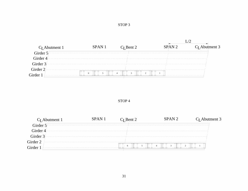
STOP 3

SPAN 1 SPAN 2

456


Girder 1Girder 2Girder 3Girder 4Girder 5

3 2 1

L/2

STOP 4

SPAN 1 SPAN 2

123

Girder 5Girder 4



6 5 4

31

SPAN 1 SPAN 2

456


Girder 1Girder 2


SPAN 1 SPAN 2Girder 5Girder 4



3 2 1

4 5 6

5685

(Dimensions in mm)

STOP 5

STOP 6

32

center for infrastructure engineering...

Documents