HAL Id: hal-01925647https://hal.archives-ouvertes.fr/hal-01925647

Submitted on 16 Nov 2018

HAL is a multi-disciplinary open accessarchive for the deposit and dissemination of sci-entific research documents, whether they are pub-lished or not. The documents may come fromteaching and research institutions in France orabroad, or from public or private research centers.

L’archive ouverte pluridisciplinaire HAL, estdestinée au dépôt et à la diffusion de documentsscientifiques de niveau recherche, publiés ou non,émanant des établissements d’enseignement et derecherche français ou étrangers, des laboratoirespublics ou privés.

Centrality metrics in dynamic networks: a comparisonstudy

Marwan Ghanem, Clémence Magnien, Fabien Tarissan

To cite this version:Marwan Ghanem, Clémence Magnien, Fabien Tarissan. Centrality metrics in dynamic networks: acomparison study. IEEE Transactions on Network Science and Engineering, IEEE, 2018, pp.1 - 1.�10.1109/TNSE.2018.2880344�. �hal-01925647�

1

Centrality metrics in dynamic networks: acomparison study

Marwan Ghanem∗, Clemence Magnien∗ and Fabien Tarissan†∗Sorbonne Universite, CNRS, Laboratoire d’Informatique de Paris 6, LIP6, F-75005 Paris, France

†Universite Paris-Saclay, CNRS, ENS Paris-Saclay, ISP UMR 7220, France

Abstract—For a long time, researchers have worked on defining different metrics able to characterize the importance of nodes in staticnetworks. Recently, researchers have introduced extensions that consider the dynamics of networks. These extensions study thetime-evolution of the importance of nodes, which is an important question that has yet received little attention in the context of temporalnetworks. They follow different approaches for evaluating a node’s importance at a given time and the value of each approach remainsdifficult to assess. In order to study this question more in depth, we compare in this paper a method we recently introduced to threeother existing methods. We use several datasets of different nature, and show and explain how these methods capture different notionsof importance.We also show that in some cases it might be meaningless to try to identify nodes that are globally important. Finally, wehighlight the role of inactive nodes, that still can be important as a relay for future communications.

Index Terms—centrality, network dynamics, temporal paths, node importance

F

1 INTRODUCTION

Scientists studying complex networks have been inter-ested for a long time in the question of evaluating theimportance of a node. This has led to the introduction ofseveral measures of importance, such as for instance degree,closeness or betweenness centrality, Eigenvector centralityor Katz centrality, or PageRank.

Many centrality measures are based on the study ofpaths in the network. In this approach, a node will beimportant if the paths from it to other nodes are short inaverage, or if it lies on the shortest paths between sev-eral pairs of nodes. One motivation is that links can actas a dissemination medium for an information spreadingon the network. For instance, individuals can exchangeinformation when they communicate, or a message can beforwarded from computer to computer until it reaches itsdestination.

Researchers started to focus on static networks first asthey represent many real-world situations, such as proteininteraction networks or food chain networks, among others.However, other cases of interest include temporal aspects,such as email exchanges between individuals occurring atdifferent points in time. Such networks were first analyzedand modeled statically for the sake of simplicity but thisrepresentation induces a strong loss of information. Indeed,in the case of path based centralities, the order of links iscompletely lost and paths that do not respect time exist inthe time-aggregated version of a dataset. To observe this,consider the toy example of Figure 1. This small networkcomposed of five nodes evolves during four distinct timesteps. By discarding the temporal aspect and aggregatingall links into a single network, we can observe that a pathfrom a to e exists although no transmission between a ande is possible in the temporal network.

This has led to a stream of works aiming at under-standing and modeling these dynamics. In particular, in thecase of centrality, some works have been concerned with

c

b

a

d

e

t=1

c

d

e

b

a

t=2

c

d

e

b

a

t=4

c

b

a

d

e

t=3 c

d

e

b

a

aggregated

Fig. 1: A small example of a dynamic network. The linksexisting at time t = 1 are shown on the top left corner, the

ones existing at t = 2 in the top right corner, and so on, andthe aggregated network is shown last.

efficiently updating the centrality values of the nodes whena change occurs in the network. In many cases however,the time scale at which the network evolves is the same asthe one at which a dissemination phenomena may occur onthe network. This is the case for instance when a diseasepropagates among individuals when they are in contact, orwhen information is disseminated by emails.

2

One very important point concerning centrality in dy-namic networks is that while paths change during thenetwork time span so does the importance of nodes. Con-sider again the toy example of Figure 1. One can see that,intuitively, the importance of node b is stronger at time t = 1than at time t = 3. Indeed, at time t = 1 it forms a bridgebetween node a and nodes c and d, thanks to the link thatexist at t = 2. This is in contrast with its situation at timet = 3 where it cannot be used as a relay anymore.

Several works have introduced extensions of centralitynotions for the case of dynamic networks. In this paper, westudy four such extensions proposed in the literature. Wecompare these extensions on several datasets from whichwe conclude that:

1) perception of the importance of a node stronglydepends on the centrality metric used, raising thequestion of the desired characteristics of a dynamiccentrality metric;

2) the dynamic of the network might be such that itis meaningless to identify nodes which are moreimportant than others;

3) metrics react differently to the different natures ofdatasets;

4) a node can be inactive (i.e. not have any links) at agiven time, yet be highly important as it may serveas a relay for future communications.

This work is organized as follows. First we present inSection 2 the existing work related to the notion of centralityin static and dynamic networks. We present in details thefour methods we study here in Section 3, before providingour methodology of comparison in Section 4. We presentthe datasets we use for the comparison in Section 5 and theresults we obtained in Section 6 before concluding the paperin Section 7.

2 RELATED WORK

Many papers have studied the importance of nodes in staticnetworks, i.e. networks that don’t evolve with time. Amongthe metrics that have been introduced, one may cite thedegree centrality, closeness centrality [1], betweenness cen-trality [2] and the Katz [3] and eigenvector centralities [4],[5]. Closeness and betweenness centralities are based onshortest paths, while the Katz centrality takes into accountpaths of all lengths between two nodes.

Some papers which have studied dynamic networkshave been concerned with efficiently computing the staticcentrality at all times. For instance, Kas et al. [6] proposean algorithm that, given distances between all pairs ofnodes and given a network change (edge appearance ofdisappearance), computes the new centrality measure byupdating the distance values rather than computing themall from scratch again. This is relevant, e.g. in contextswhere the network evolves at a much slower scale than theone on which a dissemination takes place.

One of the first methods attempting to account for theevolution of temporal networks is the snapshot method. Inthis approach, the network timeline is divided into severalperiods, and all nodes and links that exist in this period are

aggregated into a snapshot network; each snapshot is thenanalyzed separately using a static metric. Uddin et al. [7]propose a framework that, given a static centrality measure,computes it for each period. This method proves to be betterthan a static analysis. Another approach [8] studies the dy-namicity of nodes. The authors introduce two metrics whichquantify the change in importance and presence of a nodein a dynamic network. This approach is subtly but reallydifferent from a study of the time evolution of a node’simportance. Braha et al. [9] also use the snapshot approach.However, in addition to detecting important nodes, theydetect cycles as well. Similarly Tang et al. [10] consider thesame aggregation while keeping the edge order in eachsnapshot. They are thus more accurate as they only take intoaccount paths that are temporally possible. All in all, theinconvenience of these aggregation variants remain: eachcentrality value represents the centrality for a period ratherthan an exact instant, leading to information loss.

In many contexts, the dissemination phenomenon in thenetwork happens on the same time scale as the networkevolution. It then becomes necessary to consider temporalpaths [11], [12], i.e. link sequences that are time-respecting.For instance, in the dynamic network of Figure 1, there is atemporal path from node a to node c going through the link(a, b) at t = 1 and the link (b, c) at time t = 2.

Several definitions of temporal paths have been studiedin the literature. Some of them can be computed moreeasily than others. Whitbeck et al. [13] propose an efficientalgorithm to approximate the existence of paths in the mostdifficult case and show that the notion of reachability (i.e.which nodes can be reached from which nodes, and at whichtimes in the network’s time span) provides enlighteninginsight on the network’s dynamics.

Notions of centrality taking into account temporal pathshave also been introduced. Nicosia et al. [14] introduce thenotions of temporal closeness and betweenness centralities.However, their definition of a shortest path considers onlypaths whose starting point is at the beginning of a dataset’stime span.

Scholtes et al. [15], [16] introduced another approachto take into account all temporal paths. They introduceda higher order aggregation where each node represents apossible temporal path. In addition, they introduce severaltemporal centrality definitions, including a temporal cen-trality that represents a node’s importance at each instant,which is, however, too costly to compute except for smallexamples.

Another approach consists in depicting the dynamicnetwork as a static network [17], [18], by creating one copyof each node for every instant, and linking two consecutivecopies of the same node by a (directed) link. This repre-sentation allows to consider temporal paths while usingclassical centrality metrics. However, using this represen-tation is computationally expensive and remains unfeasibleparticularly for highly active datasets.

Various other propositions acknowledge that the dis-tances between nodes, and therefore, nodes’ importance,vary with time [9], [12], [19], [20], [21], [22]. However,in practice, they still represent the varying importance ofa node by a single value that is supposed to representits overall importance throughout the network global time

3

span.Several papers introduce and study variants of the Katz

or eigenvector centralities [23], [24]. Among those, Lermanet al. [25] acknowledge the fact that a node’s importancemay evolve with time, but no systematic study is conducted.Moreover, their variant relies on parameters defining whatis to be considered as relevant path lengths and path dura-tion, which complicates the analysis. Fenu et al. [26] explorethe different methods for representing a dynamic networkas a block matrix where each column/row corresponds to apair composed of a node and a time instant. They proposea method to construct such a block matrix that allows tocompute dynamic centrality metrics in an efficient way.Taylor et al. [27] introduce such a block matrix (that theycall supra-centrality matrix) and study the correspondingeigenvector centrality.

Finally, Costa et al. [28] notice that not all time instantsare equivalent in a dynamic network, and introducethe notion of time centrality. This measures how fast adissemination process can reach a significant portion of thenodes at a given time t. However, this notion is global anddoes not describe the importance of individual nodes in thedissemination process.

All in all, several papers acknowledge the fact that thetemporal evolution of networks impact the value of cen-trality measures and propose variations of standard metricsto account for the dynamics. However, and to the best ofour knowledge, very few analysis of the difference betweenthese methods have been performed. This paper intendsprecisely to contribute in this direction, by comparing fourdifferent methods that evaluate the importance of a nodebased on different criteria.

3 TEMPORAL CENTRALITY DEFINITIONS

In this section we present the four methods that we willcompare in the rest of the paper.

3.1 Temporal ClosenessThe first method was previously presented in [29]. A dy-namic network G = (V,E) consists of a set V of nodes 1 anda set E of timed links of the form (u, v, t) where u, v ∈ Vand t is a timestamp. Throughout the paper we considernetworks as undirected, i.e. a link (u, v, t) is equivalent to alink (v, u, t).

A temporal path in a dynamic network consists of:

• a starting time ts, and• a sequence of links

(v0, v1, t0), (v1, v2, t1), . . . , (vk, vk+1, tk)

such that:

1) for all i, i = 0..k − 1, ti < ti+1,2) t0 > ts.

We say that such a path is a path from v0 to vk+1 startingat time ts. Its duration is equal to tk − ts. We say that a pathfrom u to v starting at time ts is a shortest path if it has theleast duration among all paths from u to v starting at time

1. We assume that the set of nodes does not evolve with time.

ts. We define the (temporal) distance from u to v at time tsto be the duration of a shortest path from u to v starting atts, and we denote it by dts(u, v). If there is no path from uto v starting at time ts, we consider that dts(u, v) =∞.

Note that a path starting at time ts might imply waitingtimes at all nodes, including the first one, in the same waythat a person starting a train trip with connections at a giventime must wait for the train in the first station, and then ateach connecting station.

If we consider the dynamic network of Figure 1, there isa temporal path from b to d starting at time t = 1. The pathconsists of the links (b, c, 2) and (c, d, 4) and its duration is3. The temporal distance from b to d at time 1 is therefored1(b, d) = 3 (there is no path that starts at time 1 and arrivesearlier).

We recall that the closeness of a node u in a non-evolvingnetwork is defined as [1]:∑

v 6=u

1

d(u, v),

where d(u, v) is the classical graph distance.Similarly, we define the temporal closeness of a node u at

time t as:Ct(u) =

∑v 6=u

1

dt(u, v).

Note that the strict definition of Ct(u) requires to com-pute the value for each time instant t. For obvious compu-tational reasons (one of the dataset we use in this study isa record spanning 3 years), we only compute the temporalcloseness for each node every I seconds. The value of Iis equal to the median of inter-link duration (i.e. the timeseparating two consecutive links)2. We argue that this fixedfrequency is precise enough to get an accurate informationwhen compared to computing the temporal closeness atevery second.

3.2 Closeness SnapshotThe second method was proposed by Uddin et al. [7]. Inthis framework, a temporal network Gt is represented as asequence of static networks (snapshots), each to be analyzedseparately. Each static network is the aggregation of all thelinks in a given period and all the snapshots represent peri-ods of equal duration. Given a static centrality measure foreach snapshot (such as the classical definition of closeness),the framework computes this centrality for all nodes.

Note that for the comparison with the temporal closenesspresented above, we consider the closeness value of a nodeis the same every I seconds in a given snapshot. We denotethis method by SnapshotCl.

3.3 Temporal EigenvectorThe third method was presented by Taylor et al. [27]. Theyrepresent temporal networks as a supra-centrality matrix ofsize NT × NT , where N is the number of nodes and Tis the number of considered time periods. This matrix con-tains one static centrality matrix (for example an ordinary

2. The program we used to compute the metrics is publicly avail-able [30].

4

A > B = C = D = E > F︸ ︷︷ ︸centrality Relation

=⇒ 5 1 1 1 1 0︸ ︷︷ ︸ranks

Fig. 2: An example of inverse competition ranking.

adjacency matrix for the eigenvector centrality) for eachtime period. These matrices are placed on the diagonal ofthe supra-centrality matrix. Other links are added to couplethese centrality matrices with each other. The dominant vec-tor of this supra-centrality matrix would give the centralityfor each node i at each time t.

In the following, we call this method Temporal Eigenvec-tor. We will consider that each period has a duration of Iseconds.

3.4 Coverage CentralityThe fourth method was presented by Takaguchi et al. [17].It represents a temporal network as a static network whereeach temporal node consists of a pair composed of a node(of the original network) and a time instant. Consecutivepairs of the form (u, t1) and (u, t2) sharing a same nodeu are linked, and temporal links between nodes u and vat time t are represented by two links: one from (u, t) to(v, t + 1), and the symmetric link. This allows to representtemporal networks statically while keeping the temporalorder between the links. Building on this representation,the authors introduce two centrality notions. First, temporalcoverage centrality represents the importance of a temporalnode (u, t) by the fraction of pairs of nodes for which ashortest path passes through the node (u, t). A variant,called temporal boundary coverage centrality, has been defined.In this study, we only consider the temporal coveragecentrality. Preliminary results, however, revealed that bothcentralities behave quite similarly on our datasets.

4 COMPARISON

The four approaches described in the previous section pro-pose very different ways to quantify the importance of anode in a dynamic network, thus making it difficult todirectly compare the raw values. In the rest of the paperwe will therefore rely on the following additional steps tocompare the methods.

4.1 RankingEvaluating the importance of a node with respect to theothers by considering only its centrality value is difficult.Therefore, in order to obtain an intuition on the node’s rela-tive importance, we rank them at each time step with respectto their centrality values. We chose the inverse competitionranking method. In this ranking, the ranking 0 is attributedto the least central nodes, and the ranking of every nodeis equal to the number of less central nodes. Consider theexample in Figure 2, which consists of 6 nodes with theircentrality relationship in addition to their attributed ranks.The ranking 0 is attributed to F which is the least centralnode, while nodes B,C,D and E share the same ranking 1as they are all equally important. Finally, A is ranked 5.

We will use this ranking approach to compare properlythe results of the different methods.

First, given two rankings obtained by two differentmethods for the same network at the same time step, wecan compute their correlation as defined by the Kendall-Tau coefficient. This coefficient has a value in [−1, 1] thatrepresents the level of concordance between the two rankinglists. 1 stands for a perfect correlation while −1 stands fora perfect negative correlation. More precisely, we computethe difference between the number of concordant and dis-cordant pair of nodes between the two lists, a concordantpair of nodes being a pair for which the two nodes havethe same relationship in both ranking lists. So a pair (u, v)is said to be concordant if either u is ranked higher than vin both ranking lists, or u is lower than v in both rankinglists, or u has the same ranking as v in both ranking lists. Wethen normalize this value by the number of pairs in orderto obtain a final value between −1 and 1. We compute thiscorrelation at each instant to study its evolution over time.

Second, while it is interesting to know how much therankings obtained by different methods differ globally, thisdoes not provide any intuition on the difference of impor-tance attributed to any given node in particular. In order todeepen our understanding, we will therefore also computefor every node the difference between the two ranks. Ahigh difference thus indicates that the two rankings havea strong divergence regarding the importance of the con-sidered node, while a value close to 0 indicates that theyboth agree on its relative importance in the network. Wewill study the distribution of the rank difference over allpairs consisting of a node and a time instant.

4.2 Global importance

In order to provide a more comprehensive and globalperspective of the importance of all nodes at each timeinstant, we will study the number of times any given node isattributed a high (or low rank). The idea is that a node thatis consistently assigned a high rank is evaluated as globallyimportant. More formally, we define two regions, which wecall top and bottom, representing respectively the top 25%ranks and the bottom 25% ranks. Considering a networkof n nodes, a node with a ranking higher than bn ∗ 0.75cis therefore considered to be in the top region while a nodewith a ranking lower than bn∗0.25c is considered to be in thebottom region. This allows to detect immediately which arethe nodes of high or low global importance in a network 3.

Finally, we compute for each node the total durationspent in each region and we denote it by Durtop (resp.Durbot). To compute these durations, we consider that anode is present in the top or bottom region from the instantwhere we compute the centrality to the next computinginstant: given a node u ∈ V , if R(u) = (ri)i=1...k is thesequence of ranks (computed at instants i = 1..k) for u, wedefine Durtop(u) and Durbot(u) as :

Durtop(u) = I · |{i ≤ k − 1, ri ≥ bn ∗ 0.75c}| ,

Durbot(u) = I · |{i ≤ k − 1, ri ≤ bn ∗ 0.25c}| .

3. it is worth noticing that, because the inverse competition rankingmay assign the same ranking to several nodes, these regions maycontain more than or less than 25% of the nodes.

5

5 DATA SETS

In order to compare and understand the differences betweenthe different methods, we study several datasets comingfrom different contexts and presenting different character-istics:

• Enron [31]: this dataset contains the 47 088 emailsthat 151 Enron employees exchanged during approx-imately three years. It records information on thesenders, receivers, and the moment they were sent.

• Radoslaw [32]: this dataset contains 82 876 emailsexchanged by 168 employees of a mid-sized com-pany during a period of nine months in 2010. Itrecords information on the senders, receivers, andthe moment they were sent.

• Rollernet [33]: this dataset was collected during arollerblading tour in Paris in August 2006. The touris a weekly event and gathers approximately 2 500participants. Among these, 62 were equipped withwireless sensors recording when they were at acommunication distance from one another. The totaldataset duration is approximately 2 hours and 45minutes (note that there is a break of approximately30 minutes during the tour).

• Twitter (HashTags): A 22 day long twitter datasetgenerated by twitter accounts known to be associatedwith terrorist groups. Each node represents a hash-tag, while each link represents a tweet that containedthe two hashtags. Thus, a tweet with several hashtagsgenerates several links. The dataset contains 3 048hashtags and 100 429 links.

• Twitter (Retweets): From the same twitter dataset,we extracted a subset of 27 919 re-tweets generatedby the 10 484 twitter accounts. Each link (u, v, t)represents a user v re-tweeting a tweet of user u attime t.

• Facebook [34]: this dataset is a 1 year long record ofthe activity of Facebook users between 31st of De-cember 2015 and 31st of December 2016. The datasetcontains 8 977 Facebook users and their 66 153 poststo each other’s wall on Facebook. The nodes of thenetwork are users, and each link represents a userwriting on another user’s wall.

In all cases, we consider that links are undirected. Inorder to apply the snapshotCl method on these networks,we need to choose a snapshot duration. Choosing the ap-propriate value is in general a difficult question as thisimpacts the obtained results [35], [36], [37]. We chose thevalue that gave a good compromise between a low loss oftemporal information (i.e., a low aggregation and hence asmall snapshot duration) and a sufficiently high number ofactive nodes, so each snapshot contains relevant informa-tion. We show that the choice of the snapshot duration haslittle impact on our observations in Section 7 and in thesupplementary material.

The main global characteristics of these datasets, includ-ing the chosen snapshot duration, are presented in Table 1.In the rest of the paper, for the sake of brevity and becausethe observations on some datasets are similar, we will onlypresent the results on three of the datasets: Enron, RollerNet,and Twitter (HashTags). Before comparing the methods, it is

0.0001

0.001

0.01

0.1

1

0 0.2 0.4 0.6 0.8 1

Nu

mbe

r o

f n

od

es

(N

orm

aliz

ed

Logsca

le)

Duration (Normalized)

Enron RollerNet Twitter

Fig. 3: Time-evolution of the proportion of active nodes.

enlightening to make some global observation related to thedynamic of the three networks.

For each dataset, we computed the proportion of activenodes in a snapshot (i.e. the fraction of nodes having at leastone link during the corresponding period). Figure 3 showsthe time evolution of this value for the three datasets. In theEnron case, the proportion increases slowly to a maximumof 80% before dropping drastically at the very end. In theRollerNet case, the proportion of active nodes increasesrapidly and remains very close to 1 until the end. Finally, inthe Twitter dataset, we can see that the activity is extremelylow compared to the two other datasets, with only veryfew nodes active in each snapshot. Thus, those three casespresent very different characteristics in terms of activity. Weconjecture that this has a strong impact on the way node’simportance is perceived by the different methods. We willinvestigate this question in the next section.

6 RESULTS

In this section, we compare how the different methodspresented in Section 3 quantify the importance of nodesin a dynamic network. We start by analyzing the globaldifference between the methods (Section 6.1) before eval-uating how this difference impacts the relative importanceof individual nodes (Section 6.2). Finally, we compare whichnodes are identified by the methods as globally importantover the whole period of time (Section 6.3).

Note that temporal closeness, snapshotCl and temporaleigenvector have been computed for all datasets but thecoverage centrality was too computationally expensive tobe used on another dataset than Enron.

6.1 Global observations

We start by comparing temporal closeness with snapshotCl.Figure 4 presents the evolution of the Kendall-tau correla-tion between the rankings provided by the two methodsfor the three datasets. For Enron (Figure 4, top), the cor-relation is low at first and then increases over time. Atthe beginning, a large number of nodes are inactive andsnapshotCl attributes the lowest rank (0) to all of them.However, temporal paths involving links that appear laterin the dataset exist from most of these nodes. Therefore, anon-zero value (and hence a non-zero rank) is attributedby the temporal closeness to these nodes. Naturally, asthe network evolves, more nodes become active and are

6

Datasets |V | |E| Duration I (Seconds) Snapshotduration

Enron 151 47 088 3 years 960 1 weekRadoslaw 168 82 876 9 months 53 1 weekRollerNet 62 403 834 3 hours 4 1 minute

Twitter(HashTags) 3 048 100 429 22 days 16 3 hours

Twitter(Retweets) 10 484 27 919 20 days 18 1 hours

Facebook 8 977 66 153 1 year 278 1 week

TABLE 1: number of nodes |V |, number of links |E|, dataset duration, median of inter-linkduration (I) and snapshot duration for each dataset.

-0.2 0

0.2 0.4 0.6 0.8

1

0 200 400 600 800 1000 1200

Kend

all-

tau c

orr

ela

tion

Time (days)

-0.2 0

0.2 0.4 0.6 0.8

1

0 0.5 1 1.5 2 2.5 3

Kendall-

tau

corr

ela

tion

Time (hours)

-0.2 0

0.2 0.4 0.6 0.8

1

0 5 10 15 20 25

Kendall-

tau

corr

ela

tion

Time (days)

Fig. 4: Time-evolution of the Kendall-Tau correlationbetween temporal closeness and snapshotCl. Top: Enron;

Middle: Rollernet; Bottom: Twitter.

then taken into account by snapshotCl, which increases thecorrelation between the two methods4.

The effect of inactive nodes spotted above is not re-stricted to the beginning of the evolution. One might noticefor instance that the correlation drops suddenly at certaininstants, even close to the end of the trace. Manual investi-gation revealed that this corresponds to moments where asignificant number of nodes are temporarily inactive. Thisgenerates a strong difference between temporal closenessand snapshotCl for the same reason than above. We later onrefer to such instants as temporary inactive moments.

Finally, at the end of the evolution, the correlation

4. note that nodes that were active in the past but do not have anyfuture links are attributed a rank of 0 by both methods.

reaches very high values; this is due to a large number ofnodes inactive and ranked 0 by both methods, which makesit hard to have a high difference in the global rankings.

In contrast with the Enron dataset, if we now considerthe RollerNet dataset (Figure 4, middle), we can see that theKendall-tau correlation 1) fluctuates highly, 2) is globallylower, and 3) can even be negative at some instants. Thisobservation is clearly related to the high activity of the nodes(see Fig. 3). This activity leads the networks of each snapshotto be much denser than in Enron. As we highlighted in Sec-tion 2, this makes snapshotCl more likely to consider pathsthat are temporally impossible, thus leading to divergencewith temporal closeness.

Finally, we focus on the Twitter dataset (Figure 4, bot-tom). Since the dataset is the least active and contains mostlytemporary inactive moments, the correlation is pretty low.At the beginning most nodes are inactive; the number ofactive nodes becomes significant only after the 14-th day.This is why the correlation starts to increase at that time.Finally, one can identify several periods of high correlationwhich are strongly related to periods with a high number ofactive nodes (see Figure 3).

We now turn to the comparison with temporal eigen-vector. Figure 5 shows the evolution of the correlationbetween temporal closeness and temporal eigenvector forthe three datasets. For Enron (Figure 5, top), the correlationfluctuates and globally increases with time, before droppingas the total activity drops (around the 1000-th day). Thisshows that both methods are only correlated when thereis a relatively high activity. Interestingly, though we wouldexpect the correlation to increase at the very end, as previ-ously seen with snapshotCl, it actually decreases. If we nowconsider the Rollernet dataset (Figure 5, middle), we can seehow the correlation fluctuates as seen previously. We noticethat the correlation is quite low. This further indicates thatboth methods do not have the same notion of importance.Finally, for the Twitter dataset (Figure 5, bottom), we cansee how the correlation is quite low and constant, with twopeaks that correspond to a clear increase of the activity.This further shows that both methods produce differentresults when the activity is low. This is probably due tothe observation made by Fenu et al. [26] that TemporalEigenvector considers paths that do not respect time and cantherefore go backwards in time. This explains why nodesthat are permanently inactive at the end of the dataset canhave a non-zero rank.

7

-0.2 0

0.2 0.4 0.6 0.8

1

0 200 400 600 800 1000 1200

Ken

da

ll-ta

u c

orr

ela

tion

Time (days)

-0.4-0.2

0 0.2 0.4 0.6 0.8

1

0 0.5 1 1.5 2 2.5 3

Ken

da

ll-ta

u c

orr

ela

tion

Time (hours)

-0.2 0

0.2 0.4 0.6 0.8

1

0 5 10 15 20 25

Kendall-

tau c

orr

ela

tion

Time (days)

Fig. 5: Time-evolution of the Kendall-Tau correlationbetween temporal closeness and temporal eigenvector. Top:

Enron; Middle: Rollernet; Bottom: Twitter.

-0.2 0

0.2 0.4 0.6 0.8

1

0 200 400 600 800 1000 1200

Kendall-

tau

corr

ela

tion

Time (days)

Fig. 6: Time-evolution of the Kendall-Tau correlationbetween temporal closeness and coverage on Enron.

We now turn to the coverage method. Figure 6 showsthe evolution of the correlation between temporal closenessand coverage over time on Enron. One can easily noticethat, except at the very end, the correlation is rather lowduring all the evolution of the network. Since coverageand temporal closeness both consider only time respectingpaths, the divergence between the two rankings indicatesthat coverage captures another notion of importance in thedynamics, which we will discuss later. However, there is anoticeable increase at the end due to the very small numberof nodes that are active at that time. This compensatesfor the difference in the definition of importance, as beingactive becomes enough to be considered important by bothmethods.

From this first analysis, we can conclude that the correla-tion between snapshotCl and temporal closeness is strongly

0

20

40

60

80

100

-1 -0.5 0 0.5 1

Num

ber

(insta

nt,nodes)

(perc

enta

ge)

EnronRollerNet

Twitter

0

20

40

60

80

100

-1 -0.5 0 0.5 1

Num

ber

(insta

nt,nodes)

(perc

enta

ge)

Ranks (Normalized by maximum value)

0

20

40

60

80

100

-1 -0.5 0 0.5 1

Ranks (Normalized by maximum value)

Fig. 7: Inverse cumulative distribution of rank differencebetween Temporal Closeness and other methods: top:

snapshotCl; bottom Left: temporal eigenvector; bottomRight: coverage centrality.

related to the proportion of active nodes in the network.However, we provided evidence that snapshotCl has twostrong limitations: when the nodes are inactive, it is un-able to detect the importance that future connections givethem; conversely, when many nodes are active, it considersmany temporally impossible paths and therefore cannotquantify accurately the importance of the nodes. Thoughthe temporal eigenvector and coverage methods do nothave the same limitations, we have seen that they bothdetect different types of temporal importance compared totemporal closeness. We will investigate this further but it isworth noting that temporal eigenvector considers paths thatmay go backwards as well as forward in time.

6.2 Impact on individual nodes.The previous section revealed that the four approachesgenerate significantly different rankings for the importanceof nodes. This does not necessarily mean that the rankattributed to a given node is very different for two differentmethods. In order to study this aspect, this section analysesthe difference in the ranks provided by the four methods foreach node. More precisely, for each time instant and for eachnode, we compute the difference between the rank grantedby temporal closeness and the one provided by either snap-shotCl, temporal eigenvector or coverage centrality. We thenstudy the distribution of obtained values.

We start by comparing the difference between temporalcloseness and snapshotCl. Figure 7 (top) presents the inversecumulative distribution of the difference of the ranks foreach node at every instant, for the three datasets. For Enronand Twitter, the temporal closeness attributes a higher rankthan snapshotCl in more than 70% of the cases. This isin agreement with the conclusions drawn in the previoussection, and is mostly due to temporary inactive momentsduring which snapshotCl attributes a rank 0 to a node,while the temporal closeness ranks it higher. In contrast,for Rollernet which is a highly active network, the numbersof negative and positive values are more balanced. This isin contrast to what we observe when we compare temporalcloseness and temporal eigenvector (Figure 7, bottom left).

8

Except a few values in Rollernet, both methods never at-tribute the same rank.

Finally, we consider the difference between temporalcloseness and coverage centrality (Figure 7, bottom right).Interestingly, similarly to the comparison to the snapshotCl,temporal closeness tends to attribute higher ranks thancoverage centrality (around 70% of the values). Sincecoverage centrality is not affected by temporary inactivemoments, this indicates that the coverage method measuresthe importance differently.

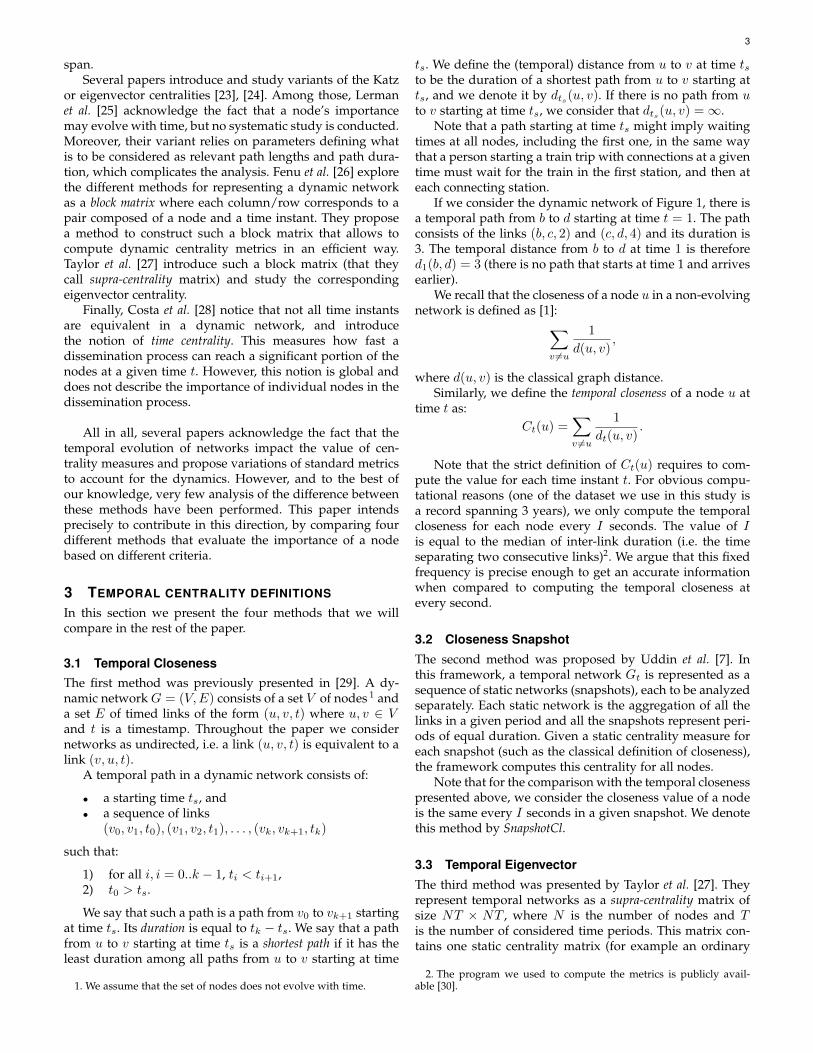
In order to illustrate the differences between the fourmethods, figure 8 presents the evolution of the rank fora given node of Enron, for the four methods. We can ob-serve that this node has many temporary inactive moments,corresponding to periods during which it snapshotCl rankis equal to 0. In contrast, temporal closeness takes into ac-count future communications and therefore attributes a rankhigher than 0 at those times. This is particularly remarkablebetween days 100 and 400. The links occurring around day400 give it a high temporal closeness and hence a high ranknot only at that time, but also influence previous times:even though the closeness at time, e.g., 300 is lower thanat time 400, it is still high enough to warrant a significantrank for this node. This is again in sharp contrast withsnapshotCl which perceives the node as unimportant forthe whole period and clearly detects the role of the nodeonly by peaks of activity. Manual investigation revealedthat this phenomenon can be frequent: the fraction of timeinstants where temporarily inactive nodes have a high rank(≥ 0.75% of the nodes) represents 10% and 20% of the totalin the Enron and Twitter cases respectively. As expected, thisproportion drops to 1% in the case of RollerNet.

In the case of temporal eigenvector, although it can de-tect the importance of inactive moments, the ranks fluctuateextremely for no apparent reason. Quite interestingly, weobserve in particular that, after the 1000-th day, althoughthis node is no longer active, its rank still fluctuates andreaches at some points very high values. This confirmswhat we mentioned at the end of Section 6.1: the temporaleigenvector method considers paths that go backwards intime (otherwise it would give a rank 0 to this node). Evenmore strikingly, we see that the importance of this nodeevolves in a non monotonic way even though it doesn’thave any activity. This indicates that this methods attributescentrality values in a non-intuitive way.

In regards to the coverage centrality, although it isdifficult to conclude on its relevance, the rank evolutionconfirms that it captures a different notion of importanceduring temporarily inactive moments. One can see in partic-ular that between days 400 and 500 the temporal closenessand coverage centrality evolve in opposite directions: thetemporal closeness rank increases as the future links getcloser, while the coverage rank decreases and drops to 0after the links have occurred.

The observations presented above confirm and refine theconclusions drawn in the previous section: not only do thefour methods give different global rankings, but they alsohave strong differences for individual nodes.

0 20 40 60 80

100 120 140 160

0 200 400 600 800 1000 1200

Ra

nkin

g

Time

Temporal Eigenvector Coverage

0 20 40 60 80

100 120 140 160

Ra

nkin

g

Temporal Closeness SnapshotCl

Fig. 8: Time-evolution of the rank of a node in Enron.

6.3 Identifying globally important nodes

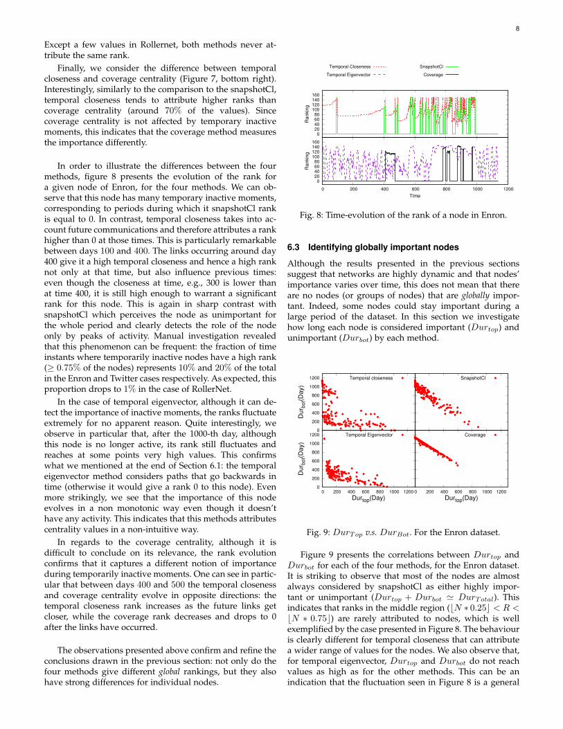
Although the results presented in the previous sectionssuggest that networks are highly dynamic and that nodes’importance varies over time, this does not mean that thereare no nodes (or groups of nodes) that are globally impor-tant. Indeed, some nodes could stay important during alarge period of the dataset. In this section we investigatehow long each node is considered important (Durtop) andunimportant (Durbot) by each method.

0

200

400

600

800

1000

1200

Dur b

ot(D

ay)

Temporal closeness

SnapshotCl

0

200

400

600

800

1000

1200

0 200 400 600 800 1000 1200

Du

r bot(D

ay)

Durtop(Day)

Temporal Eigenvector

0 200 400 600 800 1000 1200

Durtop(Day)

Coverage

Fig. 9: DurTop v.s. DurBot. For the Enron dataset.

Figure 9 presents the correlations between Durtop andDurbot for each of the four methods, for the Enron dataset.It is striking to observe that most of the nodes are almostalways considered by snapshotCl as either highly impor-tant or unimportant (Durtop + Durbot ' DurTotal). Thisindicates that ranks in the middle region (bN ∗ 0.25c < R <bN ∗ 0.75c) are rarely attributed to nodes, which is wellexemplified by the case presented in Figure 8. The behaviouris clearly different for temporal closeness that can attributea wider range of values for the nodes. We also observe that,for temporal eigenvector, Durtop and Durbot do not reachvalues as high as for the other methods. This can be anindication that the fluctuation seen in Figure 8 is a general

9

0

200

400

600

800

1000

1200

0 200 400 600 800 1000 1200

Du

r to

p C

ove

rag

e (

Da

ys)

Durtop Temporal closeness (Days)

0

200

400

600

800

1000

1200

Du

r to

p T

em

po

ral

E

ige

nve

cto

r (D

ays)

0

200

400

600

800

1000

1200

Du

r to

p S

nap

sho

tCl

(D

ays)

Fig. 10: Temporal closeness v.s. other methods. For Enrondataset.

phenomenon. Manual investigation showed that all nodesfluctuates in the same manner.

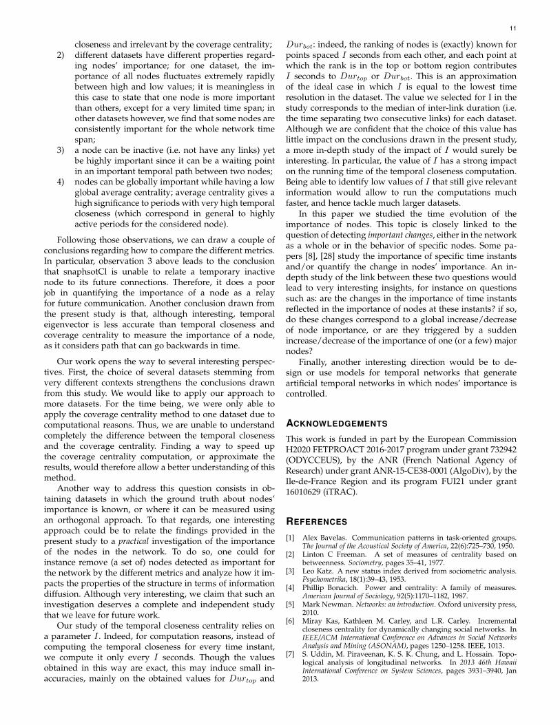
Despite these differences, one can see on Figure 10 thatthe four methods tend to perceive similarly the globalimportance of nodes; the difference between the four ap-proaches therefore lies mainly in how they evaluate unim-portant nodes, as well as the nodes of average importance.

0

0.5

1

1.5

2

2.5

3

0 0.5 1 1.5 2 2.5 3

Du

r bo

t(H

ours

)

Durtop(Hours)

Temporal Eigenvector

0

0.5

1

1.5

2

2.5

3

Du

r bo

t(H

ou

rs)

SnapshotCl

0

0.5

1

1.5

2

2.5

3

Du

r bo

t(H

ours

)

Temporal closeness

Fig. 11: DurTop v.s. DurBot. For RollerNet dataset.

Interestingly, these observations are completely differentfor RollerNet. In this dataset, one can see in Figure 11 thatno node spends time in the top (or bottom) region morethan half of the total duration, whatever the method used(except for one node that is almost always in the bottomregion). Besides, when comparing the global importanceattributed to nodes by different methods (evaluated byDurTop, Figure 12), one can see that the correlation betweentemporal closeness and the other methods is not very strongand is even anti correlated with temporal eigenvector. Allthese observations are consistent with the fact that, in thisdataset, there is no meaningful notion of global importance.We claim that this is due to the very dense (both temporallyand structurally) nature of this dataset.

The Twitter dataset is also interesting as it combines the

0

0.5

1

1.5

2

Du

r to

p S

na

psh

otC

l (

Da

ys)

0

0.5

1

1.5

2

0 0.5 1 1.5 2

Du

r to

p T

em

po

ral

E

ige

nve

cto

r (D

ays)

Durtop Temporal closeness (Days)

Fig. 12: Temporal closeness v.s. other methods. For theRollerNet dataset.

0

5

10

15

20

25

0 5 10 15 20 25

Du

r bot(D

ays)

Durtop(Days)

Temporal Eigenvector

0

5

10

15

20

25

Du

r bot(D

ays)

SnapshotCl

0

5

10

15

20

25

Du

r bot(D

ays)

Temporal closeness

Fig. 13: DurTop v.s. DurBot. For Twitter dataset.

0

2

4

6

8

10

12

0 5 10 15 20 25

Dur t

op S

napshotC

l (

Days)

Durtop Temporal closeness (Days)

Fig. 14: DurTop v.s. DurTop. For the Twitter dataset.

behaviours previously seen in Enron for the four methods.Figure 13 shows that the comparison between Durtop andDurbot is similar to what we observed on Enron, and evenmore extreme: for snapshotCl, points are all situated on theline y = T − x (where T stands for the total duration),meaning that at all times, any node is either in the top or thebottom region, but never in-between. Behaviours are morenuanced for the temporal closeness and, for temporal eigen-vector, all the nodes have very similar values. This is similarto what we observed for Enron, but far more extreme.However, in contrast with Enron, the global importance (i.e.

10

0

0.2

0.4

0.6

0.8

1

0 0.2 0.4 0.6 0.8 1Ave

rage C

losen

ess

(N

orm

aliz

ed

by

maxim

um

)

Durtop (Normalized by maximum)

Enron RollerNet Twitter

Fig. 15: Durtop v.s. average temporal closeness.

the Durtop value) attributed by temporal closeness is not atall correlated to the one attributed by the other methods (seeFigure 145).

Finally, we study the results obtained for coverage cen-trality for the Enron dataset. We observe that coverage isclose to snapshotCl in the sense that all nodes are alwayseither in the top or in the bottom region (Figure 9, bottomright). However, as pointed out before, coverage does notcapture the same notion of importance as temporal close-ness, which can be seen by comparing the correlation be-tween the DurTop values (Figure 10 bottom). The elementsprovided in this study do not allow to conclude on thereasons of this divergence and we leave this question forfurther studies.

7 DISCUSSION

In this paper, we considered four centrality methods thatquantify the time-evolution of nodes’ importance. For thecomparison of these methods, we performed several steps.This included ranking the nodes with respect to their cen-trality values, as well as computing a global duration thatrepresents a node’s global importance. Some papers [20]propose the study of the average over time of centralityrather than its evolution. They consider that this single valueis representative of the node’s complete evolution during adataset.

To assess this claim, we propose to analyze the correla-tion between Durtop and the average temporal closeness.Figure 15 presents such a correlation for the three datasets.In the case of Enron and RollerNet, these values seem corre-lated (particularly for RollerNet). However, the correlationis very low for Twitter: some nodes have a high averagetemporal closeness yet a low Durtop, and conversely. Weargue that the average temporal closeness is not represen-tative as it does not give each instant an equal amount ofimportance. As we saw, a node can have an extremely hightemporal closeness at a single instant (and therefore a highaverage temporal closeness) even though it may have a verylow activity (and hence, a very low closeness) in the rest ofthe dataset. However, the Durtop value considers that allinstants have an equal importance.

To study the snapshotCl method, we had to choose avalue for the snapshot duration. As explained in Section 5,we chose the value that gave a good compromise betweena low loss of temporal information and a sufficiently high

5. we only present the correlation between temporal closeness andsnaphsotCl as the plot obtained for temporal eigenvector is very similar.

0

200

400

600

800

1000

1200

0 200 400 600 800 1000 1200

Du

r top (

Sna

psh

otC

l)

1 day 1 week 2 weeks 1 month

0

0.5

1

1.5

2

0 0.5 1 1.5 2

Du

r top (

Sna

psh

otC

l)

30 seconds1 minute

2 minutes4 minutes

0 2 4 6 8

10 12

0 5 10 15 20 25D

ur t

op (

Snapsho

tCl)

Durtop (Temporal closeness)

1 hour2 hours

3 hours12 hours

Fig. 16: Durtop for snapshotCl v.s. Durtop for temporalcloseness for different snapshot sizes. Top: Enron; Middle:

Rollernet; Bottom: Twitter.

number of active nodes in each snapshot, so that it containsenough information. In order to check whether this has animpact on our observations, we present in Figure 16 thecorrelation between the Durtop values of temporal closenessand the one of snapshotCl for different snapshot durationsand for the three datasets we studied.

We observe few differences. The main difference is thatfor Enron, a snapshot duration significantly shorter thanthe one we studied in the rest of the paper (1 day) leadsto a somewhat smaller Durtop value for all nodes. This isconsistent with the fact that the snapshotCl method tends todetect the times at which the nodes are active: by reducingthe snapshot duration, the relative number of snapshots atwhich any given node is active diminishes, hence a decreasein the Durtop value and a corresponding increase in theDurbot value. Note that this does not affect the generalshape of the plot, and that the Durtop values attributed bytemporal closenes and snapshotCl are still correlated.

We study more in depth the impact of the snapshotduration in the supplementary material, and confirm thatthe observations made here are general and do not dependon the chosen snapshot duration.

We proposed in this paper a methodology to comparethe four methods and better understand the difference be-tween each method on different datasets of different nature.

Our observations can be summarized as follows:

1) different centralities have different results; a nodecan be perceived as important by the temporal

11

closeness and irrelevant by the coverage centrality;2) different datasets have different properties regard-

ing nodes’ importance; for one dataset, the im-portance of all nodes fluctuates extremely rapidlybetween high and low values; it is meaningless inthis case to state that one node is more importantthan others, except for a very limited time span; inother datasets however, we find that some nodes areconsistently important for the whole network timespan;

3) a node can be inactive (i.e. not have any links) yetbe highly important since it can be a waiting pointin an important temporal path between two nodes;

4) nodes can be globally important while having a lowglobal average centrality; average centrality gives ahigh significance to periods with very high temporalcloseness (which correspond in general to highlyactive periods for the considered node).

Following those observations, we can draw a couple ofconclusions regarding how to compare the different metrics.In particular, observation 3 above leads to the conclusionthat snaphsotCl is unable to relate a temporary inactivenode to its future connections. Therefore, it does a poorjob in quantifying the importance of a node as a relayfor future communication. Another conclusion drawn fromthe present study is that, although interesting, temporaleigenvector is less accurate than temporal closeness andcoverage centrality to measure the importance of a node,as it considers path that can go backwards in time.

Our work opens the way to several interesting perspec-tives. First, the choice of several datasets stemming fromvery different contexts strengthens the conclusions drawnfrom this study. We would like to apply our approach tomore datasets. For the time being, we were only able toapply the coverage centrality method to one dataset due tocomputational reasons. Thus, we are unable to understandcompletely the difference between the temporal closenessand the coverage centrality. Finding a way to speed upthe coverage centrality computation, or approximate theresults, would therefore allow a better understanding of thismethod.

Another way to address this question consists in ob-taining datasets in which the ground truth about nodes’importance is known, or where it can be measured usingan orthogonal approach. To that regards, one interestingapproach could be to relate the findings provided in thepresent study to a practical investigation of the importanceof the nodes in the network. To do so, one could forinstance remove (a set of) nodes detected as important forthe network by the different metrics and analyze how it im-pacts the properties of the structure in terms of informationdiffusion. Although very interesting, we claim that such aninvestigation deserves a complete and independent studythat we leave for future work.

Our study of the temporal closeness centrality relies ona parameter I . Indeed, for computation reasons, instead ofcomputing the temporal closeness for every time instant,we compute it only every I seconds. Though the valuesobtained in this way are exact, this may induce small in-accuracies, mainly on the obtained values for Durtop and

Durbot: indeed, the ranking of nodes is (exactly) known forpoints spaced I seconds from each other, and each point atwhich the rank is in the top or bottom region contributesI seconds to Durtop or Durbot. This is an approximationof the ideal case in which I is equal to the lowest timeresolution in the dataset. The value we selected for I in thestudy corresponds to the median of inter-link duration (i.e.the time separating two consecutive links) for each dataset.Although we are confident that the choice of this value haslittle impact on the conclusions drawn in the present study,a more in-depth study of the impact of I would surely beinteresting. In particular, the value of I has a strong impacton the running time of the temporal closeness computation.Being able to identify low values of I that still give relevantinformation would allow to run the computations muchfaster, and hence tackle much larger datasets.

In this paper we studied the time evolution of theimportance of nodes. This topic is closely linked to thequestion of detecting important changes, either in the networkas a whole or in the behavior of specific nodes. Some pa-pers [8], [28] study the importance of specific time instantsand/or quantify the change in nodes’ importance. An in-depth study of the link between these two questions wouldlead to very interesting insights, for instance on questionssuch as: are the changes in the importance of time instantsreflected in the importance of nodes at these instants? if so,do these changes correspond to a global increase/decreaseof node importance, or are they triggered by a suddenincrease/decrease of the importance of one (or a few) majornodes?

Finally, another interesting direction would be to de-sign or use models for temporal networks that generateartificial temporal networks in which nodes’ importance iscontrolled.

ACKNOWLEDGEMENTS

This work is funded in part by the European CommissionH2020 FETPROACT 2016-2017 program under grant 732942(ODYCCEUS), by the ANR (French National Agency ofResearch) under grant ANR-15-CE38-0001 (AlgoDiv), by theIle-de-France Region and its program FUI21 under grant16010629 (iTRAC).

REFERENCES

[1] Alex Bavelas. Communication patterns in task-oriented groups.The Journal of the Acoustical Society of America, 22(6):725–730, 1950.

[2] Linton C Freeman. A set of measures of centrality based onbetweenness. Sociometry, pages 35–41, 1977.

[3] Leo Katz. A new status index derived from sociometric analysis.Psychometrika, 18(1):39–43, 1953.

[4] Phillip Bonacich. Power and centrality: A family of measures.American Journal of Sociology, 92(5):1170–1182, 1987.

[5] Mark Newman. Networks: an introduction. Oxford university press,2010.

[6] Miray Kas, Kathleen M. Carley, and L.R. Carley. Incrementalcloseness centrality for dynamically changing social networks. InIEEE/ACM International Conference on Advances in Social NetworksAnalysis and Mining (ASONAM), pages 1250–1258. IEEE, 1013.

[7] S. Uddin, M. Piraveenan, K. S. K. Chung, and L. Hossain. Topo-logical analysis of longitudinal networks. In 2013 46th HawaiiInternational Conference on System Sciences, pages 3931–3940, Jan2013.

12

[8] Shahadat Uddin, Arif Khan, and Mahendra Piraveenan. A setof measures to quantify the dynamicity of longitudinal socialnetworks. Complexity, 21(6):309–320, 2016.

[9] Dan Braha and Yaneer Bar-Yam. Time-dependent complex net-works: dynamic centrality, dynamic motifs, and cycles of socialinteraction. In Adaptive networks: Theory, models and applications,pages 38–50. Springer, 2008.

[10] John Tang, Mirco Musolesi, Cecilia Mascolo, Vito Latora, andVincenzo Nicosia. Analysing information flows and key mediatorsthrough temporal centrality metrics. In Proceedings of the 3rdWorkshop on Social Network Systems, SNS ’10, pages 3:1–3:6, NewYork, NY, USA, 2010. ACM.

[11] B.-M. Bui-Xuan, A. Ferreira, and A. Jarry. Computing shortest,fastest, and foremost journeys in dynamic networks. InternationalJournal of Foundations of Computer Science, 14(2):267–285, November2003.

[12] Raj Kumar Pan and Jari Saramaki. Path lengths, correlations, andcentrality in temporal networks. Physical Review E, 84(1):016105,July 2011.

[13] John Whitbeck, Marcelo Dias de Amorim, Vania Conan, and Jean-Loup Guillaume. Temporal reachability graphs. In MOBICOM’12,pages 377–388, 2012.

[14] Vincenzo Nicosia, John Tang, Cecilia Mascolo, Mirco Musolesi,Giovanni Russo, and Vito Latora. Graph metrics for temporalnetworks. In Temporal networks, pages 15–40. Springer, 2013.

[15] Ingo Scholtes, Nicolas Wider, and Antonios Garas. Higher-orderaggregate networks in the analysis of temporal networks: pathstructures and centralities. The European Physical Journal B, 89(3):61,2016.

[16] Ingo Scholtes, Nicolas Wider, Rene Pfitzner, Antonios Garas, Clau-dio J Tessone, and Frank Schweitzer. Causality-driven slow-downand speed-up of diffusion in non-markovian temporal networks.Nature communications, 5:5024, 2014.

[17] Taro Takaguchi, Yosuke Yano, and Yuichi Yoshida. Coveragecentralities for temporal networks. The European Physical JournalB, 89(2):35, 2016.

[18] Enrico Ser-Giacomi, Ruggero Vasile, Emilio Hernandez-Garcıa,and Cristobal Lopez. Most probable paths in temporal weightednetworks: An application to ocean transport. Physical review E,92(1):012818, 2015.

[19] David A. Shamma, Lyndon Kennedy, and Elizabeth F. Churchill.Tweet the debates: Understanding community annotation of un-collected sources. In Proceedings of the First SIGMM Workshop onSocial Media, WSM ’09, pages 3–10, New York, NY, USA, 2009.ACM.

[20] Hyoungshick Kim and Ross Anderson. Temporal node centralityin complex networks. Physical Review E, 85:1–8, 2012.

[21] Ahmad Alsayed and Desmond J Higham. Betweenness in timedependent networks. Chaos, Solitons & Fractals, 72:35–48, 2015.

[22] Matthew J Williams and Mirco Musolesi. Spatio-temporal net-works: reachability, centrality and robustness. Royal Society openscience, 3(6):160196, 2016.

[23] Peter Laflin, Alexander V. Mantzaris, Fiona Ainley, Amanda Ot-ley, Peter Grindrod, and Desmond J. Higham. Discovering andvalidating influence in a dynamic online social network. SocialNetwork Analysis and Mining, 3(4):1311–1323, October 2013.

[24] Selena Praprotnik and Vladimir Batagelj. Spectral centralitymeasures in temporal networks. Ars Mathematica Contemporanea,11(1):11–33, 2015.

[25] Kristina Lerman, Rumi Ghosh, and Jeon Hyung Kang. Centralitymetric for dynamic networks. In Proceedings of the Eighth Workshopon Mining and Learning with Graphs - MLG ’10, pages 70–77, NewYork, New York, USA, July 2010. ACM Press.

[26] Caterina Fenu and Desmond J Higham. Block matrix formulationsfor evolving networks. SIAM Journal on Matrix Analysis andApplications, 38(2):343–360, 2017.

[27] Dane Taylor, Sean A. Myers, Aaron Clauset, Mason A. Porter,and Peter J. Mucha. Eigenvector-based centrality measures fortemporal networks. Multiscale Modeling & Simulation, 15(1):537–574, 2017.

[28] Eduardo C Costa, Alex B Vieira, Klaus Wehmuth, Artur Ziviani,and Ana Paula Couto Da Silva. Time centrality in dynamic com-plex networks. Advances in Complex Systems, 18(07n08):1550023,2015.

[29] Clemence Magnien and Fabien Tarissan. Time evolution of theimportance of nodes in dynamic networks. In Proceedings of theInternational Symposium on Foundations and Applications of Big Data

Analytics (FAB), in conjunction with ASONAM, 2015., FAB ’15, pages1200–1207, New York, NY, USA, 2015. ACM.

[30] Source code for the temporal centrality metrics. https://bitbucket.org/complexnetworks/closeness centrality marwan.

[31] Jitesh Shetty and Jafar Adibi. Discovering important nodesthrough graph entropy the case of Enron email database. InProceedings of the 3rd international workshop on Link discovery -LinkKDD ’05, pages 74–81. ACM Press, August 2005.

[32] Radosław Michalski, Sebastian Palus, and Przemysław Kazienko.Matching organizational structure and social network extractedfrom email communication. In Lecture Notes in Business InformationProcessing, volume 87, pages 197–206. Springer Berlin Heidelberg,2011.

[33] Pierre Ugo Tournoux, Jeremie Leguay, Marcelo Dias de Amorim,Farid Benbadis, Vania Conan, and John Whitbeck. The AccordionPhenomenon: Analysis, Characterization, and Impact on DTNRouting. In Proceedings of the 28rd Annual Joint Conference of theIEEE Computer and Communications Societies (INFOCOM), pages1116–1124. IEEE, 2009.

[34] Bimal Viswanath, Alan Mislove, Meeyoung Cha, and Krishna PGummadi. On the evolution of user interaction in facebook. InProceedings of the 2nd ACM workshop on Online social networks, pages37–42. ACM, 2009.

[35] R. Sulo, T. Berger-Wolf, and R. Grossman. Meaningful selectionof temporal resolution for dynamic networks. In Proceedings of theEighth Workshop on Mining and Learning with Graphs, 2010.

[36] S. Uddin, N. Choudhury, S. M. Farhad, and M. T. Rahman.The optimal window size for analysing longitudinal networks.Scientific Reports, 7(1):13389, 2017.

[37] Yannick Leo, Christophe Crespelle, and Eric Fleury. Non-alteringtime scales for aggregation of dynamic networks into series ofgraphs. In International Conference on emerging Networking EXperi-ments and Technologies (CONEXT), 2015.

Marwan Ghanem is a Ph.D. candidate at theComputer Science laboratory LIP6 (SorbonneUniversite/CNRS). He received his Master ofScience degree in Computer Science from Uni-versity Pierre and Marie Curie in 2015. His re-search area is the study of real complex net-works and he focuses in particular on analysingthe importance of their nodes.

Clemence Magnien is a senior researcher atCNRS and member of the LIP6 lab (SorbonneUniversite/CNRS). She completed her PhD incomputer science from Ecole Polytechnique in2003, and joined LIP6 in 2007.

Her research area is the study of large graphsoccurring in practice, both in computer sciencebut but also coming from other contexts, likesocial or biological networks.

Fabien Tarissan is a permanent researcher atCNRS and member of the laboratory ISP at ENSParis-Saclay. He was previously an associateprofessor at Sorbonne Universite from 2009 to2015. His work mainly concerns the analysisand modeling of large networks encountered inpractice. His approach consists in proposing newtheoretical tools in order to identify non-trivialproperties of these networks and to define newmodels able to capture these properties.

1

Supplementary material

F

In this supplementary material we study more in depththe impact of the choice of the snapshot duration for thesnapshotCl method.

For each of the datasets, we chose a range of values forthe snapshot duration, some shorter and some larger thanthe one we have chosen for the main part of the paper. Thenwe make the same studies than in Section 6 of the mainpaper.

−0.2 0

0.2 0.4 0.6 0.8

1

0 200 400 600 800 1000 1200

Kendall

Corr

ela

tion

Duration

1 day 1 week 2 weeks 1 month

−0.2 0

0.2 0.4 0.6 0.8

1

0 0.5 1 1.5 2 2.5 3

Kendall C

orr

ela

tion

Duration

30 seconds

1 minute

2 minutes

4 minutes

−0.2 0

0.2 0.4 0.6 0.8

1

0 5 10 15 20 25

Kendall C

orr

ela

tion

Duration

1 hour

2 hours

3 hours

12 hours

Fig. 1: Time-evolution of the Kendall-Tau correlationbetween temporal closeness and snapshotCl for different

snapshot sizes. Top: Enron; Middle: Rollernet; Bottom:Twitter.

Figure 1 shows the time evolution of the Kendall-taucorrelation between the rankings produced by snapshotCland temporal closeness, for the three datasets.

We observe the same global behaviors for all snapshotdurations. In particular, we still observe a global increase ofthe correlation for the Enron dataset, coming from the factthat, as less nodes are active at the end of the dataset, bothmethods tend to agree more on which nodes are important;we still observe very important fluctuations for the Roller-

Net dataset, consistent with the fact that this dataset is verydense and importance fluctuates widely from one instant tothe next; and we still observe a consistently low correlationfor the Twitter dataset, except at the times at which a largerfraction of nodes are active.

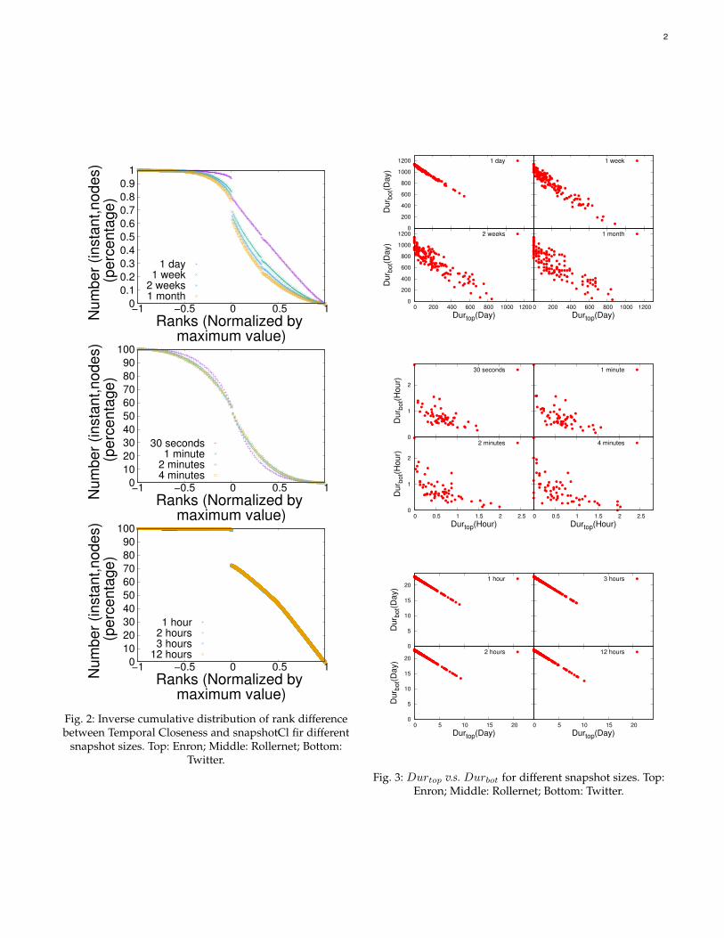
We now study the difference in the ranks attributed bysnapshotCl and temporal closeness to each node. Figure 2presents the inverse cumulative distribution of the differ-ence of the ranks for each node at every instant, for thethree datasets.

For Rollernet and Twitter, we observe no significantdifferences for the different snapshot durations. For En-ron, we observe that, the higher the snapshot duration,the lower the fraction of (instant, node) pairs for whichtemporal closeness attributes a higher rank than snapshotCl.This is consistent with our earlier observations: snapshotClattributes a rank of 0 during temporary inactive momentsto the corresponding nodes, while temporal closeness ranksthem higher. Since increasing the snapshot duration reducesthe fraction of snapshots during which any given node isinactive, this induces a smaller fraction of positive rankdifferences.

Finally, Figure 3 presents the correlations betweenDurtop and Durbot values for snapshotCl, for the threedatasets. Again, for Rollernet and Twitter, we observe nosignificant difference: for Rollernet, we see that the valuesbecome more scattered when the snapshot duration in-creases; for Twitter however, the values are still concentratedin a single line, meaning that snapshotCl always considersa node as important or unimportant, but never places it inthe middle region.

For Enron, we observe that the values become signif-icantly more scattered as the snapshot duration increases.This comes from the fact that, as the snapshot durationincreases, a larger fraction of nodes become active in eachsnapshot, and hence not all active nodes are placed in thetop region by snapshotCl. However, we still clearly observethe tendency to seldom place nodes in the middle region,characterized by a globally linear shape of the plot, evenfor large snapshot durations: a one month snapshot leadsto approximately 36 snapshots for the whole dataset, whichinduces a very important loss of temporal information.

Finally, as we observed in the main text of this paper,the snapshot duration has little impact on the correlationsbetween the Durtop values of snapshotCl and temporalcloseness.

2

0

0.1

0.2

0.3

0.4

0.5

0.6

0.7

0.8

0.9

1

−1 −0.5 0 0.5 1

Num

ber

(insta

nt,nodes)

(perc

enta

ge)

Ranks (Normalized by maximum value)

1 day1 week

2 weeks1 month

0

10

20

30

40

50

60

70

80

90

100

−1 −0.5 0 0.5 1

Num

ber

(insta

nt,nodes)

(perc

enta

ge)

Ranks (Normalized by maximum value)

30 seconds1 minute

2 minutes4 minutes

0

10

20

30

40

50

60

70

80

90

100

−1 −0.5 0 0.5 1

Num

ber

(insta

nt,nodes)

(perc

enta

ge)

Ranks (Normalized by maximum value)

1 hour2 hours3 hours

12 hours

Fig. 2: Inverse cumulative distribution of rank differencebetween Temporal Closeness and snapshotCl fir different

snapshot sizes. Top: Enron; Middle: Rollernet; Bottom:Twitter.

0

200

400

600

800

1000

1200

Dur b

ot(D

ay)

1 day

1 week

0

200

400

600

800

1000

1200

0 200 400 600 800 1000 1200

Du

r bot(D

ay)

Durtop(Day)

2 weeks

0 200 400 600 800 1000 1200

Durtop(Day)

1 month

0

1

2

Du

r bot(H

our)

30 seconds

1 minute

0

1

2

0 0.5 1 1.5 2 2.5

Dur b

ot(H

our)

Durtop(Hour)

2 minutes

0 0.5 1 1.5 2 2.5

Durtop(Hour)

4 minutes

0

5

10

15

20

Dur b

ot(D

ay)

1 hour

3 hours

0

5

10

15

20

0 5 10 15 20

Dur b

ot(D

ay)

Durtop(Day)

2 hours

0 5 10 15 20

Durtop(Day)

12 hours

Fig. 3: Durtop v.s. Durbot for different snapshot sizes. Top:Enron; Middle: Rollernet; Bottom: Twitter.