centre for advanced s pa tial analysis
TRANSCRIPT

CE
NT
RE
FO
R A
DVA
NC
ED
SP
AT
IAL
AN
AL
YS
ISW
orkin
g P
aper
Ser
ies
Paper 20
HOW LAND-USE-TRANSPORTATION
MODELS WORK
Paul M. T orrens

Centre for Advanced Spatial Analysis
University College London
1-19 Torrington Place
Gower Street
London WC1E 6BT
Tel: +44 (0) 20 7679 1782
Fax: +44 (0) 20 7813 2843
Email: [email protected]
http://www.casa.ucl.ac.uk
http://www.casa.ucl.ac.uk/working_papers.htm
Date: April 2000 (edited for style November 2000)
ISSN: 1467-1298
© Copyright CASA, UCL.
3
ABSTRACT ..................................................................................................................................................6
1 INTRODUCTION .................................................................................................................................6
2 WHY LAND-USE–TRANSPORTATION MODELS? .............................................................................7
2.1 JUSTIFYING URBAN SIMULATION ............................................................................................................7
2.2 THE EMERGENCE OF URBAN MODELLING.................................................................................................8
3 MODEL CLASSIFICATION ................................................................................................................9
3.1 BASIC MODELS....................................................................................................................................9
3.2 MATHEMATICAL MODELS ...................................................................................................................10
3.3 LAND-USE–TRANSPORTATION MODELS.................................................................................................11
4 DESCRIPTIVE AND ANALYTICAL URBAN MODELS .....................................................................11
4.1 THE VON THUNEN MODEL...................................................................................................................11
4.2 CONCENTRIC ZONE THEORY................................................................................................................13
4.3 WEDGE OR RADIAL SECTOR THEORY.....................................................................................................14
4.4 MULTIPLE-NUCLEI THEORY.................................................................................................................15
5 GENERAL STRUCTURE OF THE LAND-USE–TRANSPORTATION MODEL ..................................16
6 MODELLING TECHNIQUES ............................................................................................................17
6.1 SPATIAL INTERACTION MODELS...........................................................................................................18
6.1.1 Production constraints..............................................................................................................21
6.1.2 Attraction constraints...............................................................................................................22
6.1.3 Production-attraction constraints...............................................................................................23
6.1.4 Entropy-maximizing models.......................................................................................................24
6.2 SPATIAL CHOICE MODELS...................................................................................................................28
6.2.1 Discrete choice models.............................................................................................................28
6.2.2 Non-hierarchical logit models....................................................................................................30
6.2.3 Nested logit models..................................................................................................................31
6.3 BID-RENT THEORY.............................................................................................................................33

4
7 INDIVIDUAL MODEL COMPONENTS (SUB-MODELS) ...................................................................34
7.1 THE LAND USE SYSTEM.......................................................................................................................35
7.1.1 Location.................................................................................................................................35
7.1.2 The land development process....................................................................................................41
7.1.3 Supply, demand, and equilibrium................................................................................................43
7.2 THE TRANSPORT SYSTEM....................................................................................................................45
7.2.1 Potential demand modelling and trip generation...........................................................................46
7.2.2 Trip distribution.......................................................................................................................47
7.2.3 Modal split..............................................................................................................................48
7.2.4 Trip assignment (route choice)...................................................................................................48
7.2.5 Accessibility............................................................................................................................49
7.2.6 Generalized costs of travel........................................................................................................53
7.3 INTEGRATING LAND USE AND TRANSPORTATION.....................................................................................54
7.4 SIMULATING PLANNING AND PUBLIC POLICY ..........................................................................................55
8 THE FAILURES OF LAND-USE–TRANSPORTATION MODELS ......................................................56
8.1 THE UNDOING OF URBAN MODELING.....................................................................................................56
9 IN DEFENSE OF URBAN MODELLING ............................................................................................57
9.1 URBAN MODELS WEATHER THE STORM.................................................................................................57
9.2 ADVANCING URBAN MODELLING .........................................................................................................59
9.2.1 Dynamics................................................................................................................................59
9.2.2 Detail.....................................................................................................................................60
9.2.3 Interfacing with the user............................................................................................................60
9.2.4 Flexibility................................................................................................................................60
9.2.5 Behavioural realism.................................................................................................................61
9.2.6 Zonal geography......................................................................................................................61
10 CONCLUSIONS.................................................................................................................................62
10.1 WEAVING COMPLEXITY INTO THE SIMULATION FRAMEWORK....................................................................62

5
10.2 ENGAGING THE USER THROUGH VISUALIZATION AND APPLICATION...........................................................65
10.3 CONCLUSIONS..................................................................................................................................66
REFERENCES ...........................................................................................................................................68

6
ABSTRACT
This working paper serves as an introductory reference for those studying the application of land-use–transportation models to the simulation of urban systems. The paper is by no meanscomprehensive, but aims to provide the reader with a foundation in the basic principles underlyingland-use–transportation models and to set those principles in the context of urban management andurban studies. The paper opens with taxonomy of urban simulation models and a treatment ofdescriptive and analytical models. This serves to situate land-use–transportation models in thecontext of a broader simulation environment. The paper then reviews land-use–transportationmodels according to their simulation techniques and individual components. Towards the secondhalf of the paper, the discussion moves to a critical overview of urban simulation and deals withmodel weaknesses and strengths in a holistic fashion, before concluding with a discussion of someinnovations in academic research that are likely to shape future models.
1 INTRODUCTION
Computer simulation models combine theory, data, and algorithms to arrive at an abstract
representation of the character and functioning of the land-use–transportation system. Ideally, once
a simulation has been calibrated against a known scenario, the model may be used to make
predictions about the future state of that system. Land-use–transportation models are a particular
class of model used to simulate how land-use and transportation systems operate. They were first
put to use in the management of urban systems to facilitate long-range planning, to simulate the
potential outcomes of decisions affecting the cities, and as a laboratory for testing ideas and
hypotheses relating to urban systems. Since their inception, they have steadily grown in
sophistication and their use has become widespread. However, land-use–transportation models are
uncertain tools—as with any model there is a degree of abstraction in their representation of real-
world systems and processes. Urban simulation is also a relatively unique modelling problem. The
urban systems commonly represented in urban models—economic, social, and environmental—are
notoriously difficult to simulate. Land-use–transportation models are often used to support
decisions that have profound influences upon people’s lives. Also, policies and ideas about the city
are often difficult to experiment with. Equally, the pace of change in urban areas is often such that
models have a hard time keeping up with the phenomena they are simulating.
In the past, researchers and model developers were restricted by their theoretical knowledge about
the city and how it might be simulated as well as being constrained by technological limitations.
Nevertheless, the simulation environment is now appropriate for the infusion of new ideas into
urban modelling. This paper is intended to serve as an introduction to land-use–transportation
models at a pace and level of detail that will make them accessible to the reader as well as serving

7
as a reference resource.1 The paper deals largely with the techniques that are most prevalent in
operational land-use–transportation models, simply because those ideas form an important
foundation on which to advance urban modelling. Some new emerging techniques in academic
research are introduced, however.
The paper proceeds in Section 2 with a brief overview of modelling and a treatment of the
introduction of models in planning. Taxonomy of models is then developed in Section 3, setting
land-use–transportation models in the context of a broader simulation environment. Some important
descriptive and analytical urban models are mentioned in Section 4, followed by an introduction to
the general structure of the land-use–transportation model in Section 5. Some key modelling
techniques are described in detail in Section 6, providing the reader with a foundation in the
simulation methods that will feature in subsequent sections. Individual model components are then
discussed in Section 7, beginning with the land-use system, and followed by the transport system
and integrated methods for representing the two. In Section 8 the paper moves into a discussion of
the relative merits and shortcomings of land-use–transportation modelling and concludes in Section
9 with a consideration of the future of urban simulations.
2 WHY LAND -USE–TRANSPORTATION MODELS ?
2.1 JUSTIFYING URBAN SIMULATION
There are some powerful rationales for applying simulation models to the study and management of
urban systems. In Europe, concerns about the sustainability of our cities is driving a concerted effort
to model their functioning in a bid to forecast future urban patterns. Meanwhile, in the United States
there exists legislation that both directly and indirectly encourages the development of simulation
models of various urban phenomena. This legislation includes the Clear Air Act Amendments:
1 For a more thorough review of specific operational models, the reader is referred to Barra, 1989; Cambridge
Systematics, 1991; Government of Ireland, 1995; Landis, 1994, 1995; Landis and Zhang, 1998; Miller et al., 1998;
Oryani and Harris, 1996; Putman, 1989, 1992; Waddell, 1998a, 1998b; Wegener, 1983, 1994, 1996. For general
treatments of modelling principles, see Batty 1976; Putman 1979, 1983; Barra 1989; Fotheringham and O'Kelly 1989;
Putman 1989; Cambridge Systematics and Group 1991; Putman 1992; Government of Ireland 1995; Oryani and Harris
1996; Australian Bureau of Transportation Economics 1998; Miller, Kriger et al. 1998; Fotheringham, Brunsdon et al.
2000.

8
CAAA (1990), the Intermodal Surface Transportation Efficiency Act: ISTEA (1991), and ISTEA’s
successor, the Transportation Equity Act for the Twenty First Century: TEA-21 (1997).
CAAA, ISTEA, and TEA-21 incorporate legislative provisions that mandate land-use–
transportation modelling mostly in its capacity to serve as decision support systems for policies
designed to mitigate urban air problems. However, other initiatives—such as the Travel Model
Improvement Program: TMIP (1992), which was established by the Federal Highway
Administration; the Federal Transit Administration; the Office of the Secretary, U.S. Department of
Transportation; and the U.S. Environmental Protection Agency—have been introduced specifically
to encourage improvements in land-use–transportation modelling.
Other justifications for urban simulation models include the functionality that they offer by
allowing us to test theories and practices about urban systems in a controlled computer
environment. Proceeding from a simulation model, we can evaluate the merits of theories relating to
urban phenomena and test the application of policy measures (such as growth management,
congestion pricing, and pollution mitigation schemes) to various scenarios for urban futures.
2.2 THE EMERGENCE OF URBAN MODELLING
Before proceeding with a discussion of the mechanics of land-use–transportation models, it is
perhaps useful to begin with a review of their history and the academic and social environments that
spawned their introduction into urban planning.
Modelling first became widely applied to urban planning at the beginning of the 1960s. Its adoption
coincided with a general transformation of the character of planning as one identified as
architecture-writ-large to one rooted less intuitively but grounded more objectively (Batty, 1994). In
short, urban modelling emerged as part of an effort to better quantify and mathematically represent
the conditions upon which decisions were made. To facilitate this, model developers, began to
poach analytical methodologies from other disciplines—human ecology, mathematics, geography,
operations research, linear programming, regional science, and economics—modellers were
relentless in their pilfering of scientific techniques that might be applied to urban phenomena. There
were a number of motivating forces driving these changes.
The 1960s was a time of insecurity about the intellectual credentials of urban studies (including
both urban geography and urban planning) as a social science (Sayer, 1979). While neighbouring
9
disciplines were quantifying heavily over this period, modelling was, in a sense, a bandwagon
which urban studies researchers felt compelled to jump on in a bid to legitimize the scholarly merits
of their academic pursuits and professional activities.
Underlying and supporting this motivation was a sense of “technological optimism” (Klosterman
1994). Urban models were first used in a period in which it was felt that the scientific successes of
the time (telecommunications, medicine, agriculture, physics, chemistry, and, of course, computers)
could be applied as efficiently and, it was hoped, as successfully to the social realm.
At full swing in their popularity by the early-1960s, urban models were being developed for several
cities in the United States. Large-scale modelling projects were funded in Pittsburgh, San Francisco,
the Penn-Jersey corridor, and elsewhere. Models were also developed for several European cities.
At first they were introduced with the aim of solving land-use and transportation questions, later
being employed with the goal of addressing a wider range of urban problems.
3 M ODEL CLASSIFICATION
3.1 BASIC MODELS
Of course, urban models come in many flavours. These range in variety from basic to mathematical
in character, with a respective diversity of theoretical foundations, purposes, and functionality of
use. Nevertheless, a general taxonomy of urban models is presented here as a framework within
which the reader can situate land-use–transportation models. Basic models rarely contain the
capacity for prediction. They may be classified into three main groups: scale, analogue, and
conceptual.
Also known as iconic, scale models are amongst the most well known models. Broadly speaking,
they are scaled-down versions of reality, usually without any functional or predictive capacity.
Essentially, they differ from reality only in size. Examples include wooden block models and
architectural mock-ups.
In analogue models, size is transformed, but so are some of the properties of the thing that is
actually being modelled. The most familiar analogue model, in a geographic sense, is the map. Here
size is reduced (as with the scale model), but so also are some of the properties of the thing being
modelled. For example, in a map scale is reduced, but features are also symbolized (Thomas and
Huggett, 1980).
10
A conceptual model generally expresses how we think a system works. Usually, conceptual models
are presented as arrows that illustrate links or relationships, and boxes representing system
components.
3.2 MATHEMATICAL MODELS
Mathematical models take the ideas encapsulated in a conceptual model and transform them into
mathematical symbology, enabling conceptual ideas to be tested (and in some cases, permitting
predictions to be made). The validity of mathematical models can then be evaluated by comparing
their predictions against observed data. Under the heading of mathematical models there exist a
myriad of sub-classifications, with a variety of goals and techniques. At the broadest level, we can
consider mathematical models to be either normative or deterministic in their goals.
Normative models proceed with assumptions about how a system ought to behave. Deterministic
models, on the other hand, proceed on the assumption that natural, physical laws control the
behaviour of the system being simulated; and that once these laws have been uncovered, the
behaviour of the system can be predicted. As with predictive models, deterministic models are
loosely based on a set of behavioural relationships. Their application to the land-use–transportation
problem is usually concerned with accounting for changes in the spatial pattern of land-use and
transportation systems. They may also be employed to predict or assess the impacts of changes in
exogenous variables or in policies targeted at those systems (Government of Ireland, 1995). Two
important sub-classes of predictive model are probabilistic and optimzing models.
Probabilistic models are deterministic in their assumptions, but are distinct from the broad class of
predictive models in that they express the initial assumptions of the model as a set of probabilities.
In this sense they infuse an element of chance into the simulation process, so that predictions made
by probability models are stated with a known degree of error or tolerance. In this way, probabilistic
models focus on a range of possible outcomes rather than single predictions (Thomas and Huggett,
1980).
Optimizing models apply optimization theory to urban simulation—they assume that the
distribution of urban activities can be allocated so as to optimize some objective function (e.g., the
cost of transportation). The models generally have constraints placed on them to ensure that the
system being simulated matches what can be observed.

11
3.3 LAND-USE–TRANSPORTATION MODELS
Land-use–transportation models belong to the mathematical family of models. They are composed
of independent land-use and travel models, with mechanisms for coupling the two—either loosely
or in a more integrated fashion.
Land-use models are used to predict demographic and economic measures of land-based activities.
These measures describe the population (usually in terms of income and employment) and built-
space environment (e.g., floor space) for a given urban area.
Travel models (specifically, travel demand models) are used to predict travel patterns on a
transportation network. This class of models aim to simulate travel patterns as a function of human
activities (commonly considered in terms of land uses) as well as the characteristics of the transport
network (commonly considered in terms of accessibility)(Miller et al., 1998).
Integrated land-use–transportation models are used to simulate the interaction of the land use
system and the transport system. Generally, this interaction is simulated by means of feedback
mechanisms. The nature of this interaction will be explored further in later sections.
4 DESCRIPTIVE AND ANALYTICAL URBAN MODELS
Much of the contemporary land-use–transportation modelling effort has proceeded on a foundation
of descriptive or analytical models that have been steadily developed since the beginning of the
Twentieth Century. Among the more influential of these have been the von Thunen model,
concentric zone theory, wedge or radial sector theory, and multiple-nuclei theory. While many of
these models are weak in their theoretical justifications, outmoded in their capacity to describe
today’s cities, and limited in their predictive powers; they have provided both an important
environment for urban simulation and a base upon which contemporary efforts can be built. The
important differentiating factor between descriptive or analytical models and land-use–
transportation models is that descriptive or analytical models offer explanations as to how various
urban phenomena emerge, but they generally abstract from questions of why those patterns
materialize.
4.1 THE VON THUNEN MODEL
Based on a series of simplifying assumptions, von Thunen described a model that would account for
a spatial distribution of sites across a theoretical geographic area that would have varying rent-
12
generating capacities dependent upon transportation costs and distance from a central site. Von
Thunen’s model was highly generalized and was based on a series of simplifying assumptions
(Krugman, 1996):
1. The space in which the model was framed was assumed to be an infinite or boundless, flat,
and featureless plane, over which climatic conditions and natural resources were uniformly
distributed
2. The central attracting area was assumed to be a central market
3. Transportation to this central market was assumed to be by horse and cart
4. An allowance for the production and sale of different goods was made, but these goods were
regarded as differing in bulk, therefore having varying costs of transportation from point of
production to the central market
5. For each of these products, transport costs were assumed to vary with distance from the point
of production to the point of sale at the central market
6. The profits to be gleaned from the cultivation of one hectare of land were assumed to be the
same for each product
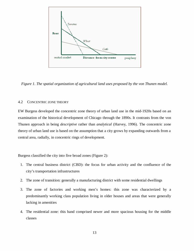
Based on these assumptions, and operating over the hypothetical space that von Thunen proposed,
he argued that agricultural land uses would segregate into a spatially hierarchic structure akin to that
demonstrated in Figure 1. (As we will see later, the idea is not at all different from bid-rent theory,
which draws heavily from the von Thunen model in inspiration.)
13
Figure 1. The spatial organization of agricultural land uses proposed by the von Thunen model.
4.2 CONCENTRIC ZONE THEORY
EW Burgess developed the concentric zone theory of urban land use in the mid-1920s based on an
examination of the historical development of Chicago through the 1890s. It contrasts from the von
Thunen approach in being descriptive rather than analytical (Harvey, 1996). The concentric zone
theory of urban land use is based on the assumption that a city grows by expanding outwards from a
central area, radially, in concentric rings of development.
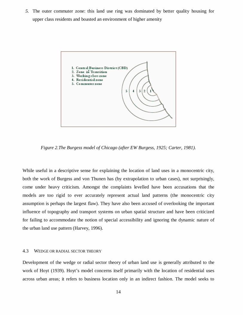
Burgess classified the city into five broad zones (Figure 2):
1. The central business district (CBD): the focus for urban activity and the confluence of the
city’s transportation infrastructures
2. The zone of transition: generally a manufacturing district with some residential dwellings
3. The zone of factories and working men’s homes: this zone was characterized by a
predominantly working class population living in older houses and areas that were generally
lacking in amenities
4. The residential zone: this band comprised newer and more spacious housing for the middle
classes
14
5. The outer commuter zone: this land use ring was dominated by better quality housing for
upper class residents and boasted an environment of higher amenity
Figure 2.The Burgess model of Chicago (after EW Burgess, 1925; Carter, 1981).
While useful in a descriptive sense for explaining the location of land uses in a monocentric city,
both the work of Burgess and von Thunen has (by extrapolation to urban cases), not surprisingly,
come under heavy criticism. Amongst the complaints levelled have been accusations that the
models are too rigid to ever accurately represent actual land patterns (the monocentric city
assumption is perhaps the largest flaw). They have also been accused of overlooking the important
influence of topography and transport systems on urban spatial structure and have been criticized
for failing to accommodate the notion of special accessibility and ignoring the dynamic nature of
the urban land use pattern (Harvey, 1996).
4.3 WEDGE OR RADIAL SECTOR THEORY
Development of the wedge or radial sector theory of urban land use is generally attributed to the
work of Hoyt (1939). Hoyt’s model concerns itself primarily with the location of residential uses
across urban areas; it refers to business location only in an indirect fashion. The model seeks to

15
explain the tendency for various socio-economic groups to segregate in terms of their residential
location decisions. In appearance, Hoyt’s model owes a great deal to Burgess’s concentric zone
model: Hoyt presents wedge-like sectors of dominant urban land use, within which he identifies
concentric zones of differential rent. The model suggests that, over time, high quality housing tends
to expand outward from an urban centre along the fastest travel routes. In this way, Hoyt transforms
Burgess’s concentric zones into radial or sectoral wedges of land use (Figure 3).
Figure 3. Hoyt’s sector model (after H. Hoyt, 1939; Carter, 1981).
The innovative element in Hoyt’s model was in considering direction, as well as distance, as a
factor shaping the spatial distribution of urban activity. Hoyt’s model also goes further than its
predecessors in recognizing that the CBD is not the sole focus of urban activity (Kivell, 1993). One
major criticism, however, is that the model overlooks the location of employment, which itself is
the major determinant of residential location (Harvey, 1996).
4.4 MULTIPLE-NUCLEI THEORY
The work of Harris and Ullmann (1945) in developing a multiple-nuclei theory of urban land use is
amongst the most innovative descriptive or analytical urban models. Their model is based on the
premise that large cities have a spatial structure that is predominantly cellular. This, they explain, is
a consequence of cities’ tendencies to develop as a myriad of nuclei that serve as the focal point for
agglomerative tendencies. Harris and Ullmann propose that around these cellular nuclei, dominant
land uses and specialized centres may develop over time.
16
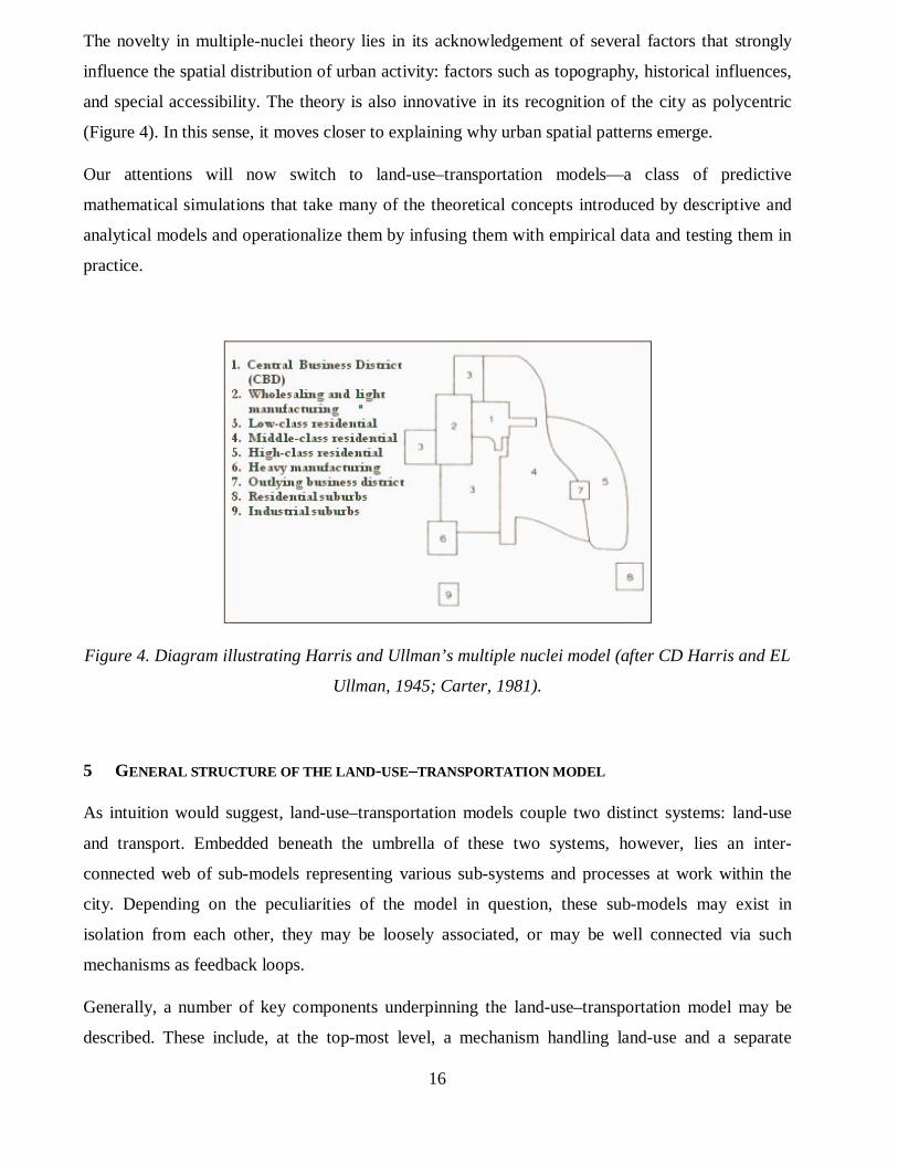
The novelty in multiple-nuclei theory lies in its acknowledgement of several factors that strongly
influence the spatial distribution of urban activity: factors such as topography, historical influences,
and special accessibility. The theory is also innovative in its recognition of the city as polycentric
(Figure 4). In this sense, it moves closer to explaining why urban spatial patterns emerge.
Our attentions will now switch to land-use–transportation models—a class of predictive
mathematical simulations that take many of the theoretical concepts introduced by descriptive and
analytical models and operationalize them by infusing them with empirical data and testing them in
practice.
Figure 4. Diagram illustrating Harris and Ullman’s multiple nuclei model (after CD Harris and EL
Ullman, 1945; Carter, 1981).
5 GENERAL STRUCTURE OF THE LAND -USE–TRANSPORTATION MODEL
As intuition would suggest, land-use–transportation models couple two distinct systems: land-use
and transport. Embedded beneath the umbrella of these two systems, however, lies an inter-
connected web of sub-models representing various sub-systems and processes at work within the
city. Depending on the peculiarities of the model in question, these sub-models may exist in
isolation from each other, they may be loosely associated, or may be well connected via such
mechanisms as feedback loops.
Generally, a number of key components underpinning the land-use–transportation model may be
described. These include, at the top-most level, a mechanism handling land-use and a separate

17
model to describe transport. The land-use module depends, in varying degrees; on sub-models for
location, land development, and an equilibrium mechanism that balances forces of demand and
supply. The transport system is traditionally simulated via a four-step process beginning with
potential demand modelling and trip generation, proceeding through trip distribution and modal
split, and concluding with trip assignment (Figure 5).
Figure 5. The general structure of a land-use–transportation model.
6 M ODELLING TECHNIQUES
The discussion of land-use–transportation models will now proceed with a summary of some of the
key mathematical principles that form the mechanics of most simulations, followed by a detailed
treatment of the various components that comprise the generic model. In Section 6.1 we discuss
spatial interaction models in both their basic and constrained forms. Section 6.2 deals with spatial
choice models. Section 6.3 then shifts the discussion to bid-rent models.
18
6.1 SPATIAL INTERACTION MODELS
The main engine of the generic land-use–transportation model has traditionally been the spatial
interaction model or variants thereof. The spatial interaction model features in land-use–
transportation simulation in its representation of flows of both trips and activities between areas of
the city. While many contemporary simulation packages are moving away from spatial interaction
modelling as a baseline simulation technique, it is worth examining the assumptions and
mathematics underpinning its application to land-use–transportation models, as the technique is still
quite widely used in practice.
A spatial interaction model is generally employed to predict the size and direction of spatial flows
using independent variables that measure some structural property of the spatial area being
modelled. For example, the spatial pattern of journey-to-work flows might be predicted using
structural variables such as the distribution of workers, the distribution of employment, and the
costs of travelling to work.
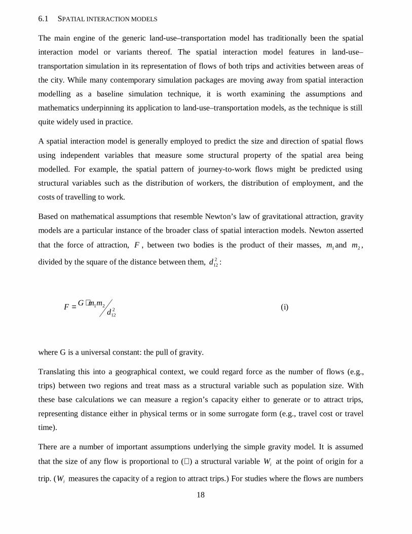
Based on mathematical assumptions that resemble Newton’s law of gravitational attraction, gravity
models are a particular instance of the broader class of spatial interaction models. Newton asserted
that the force of attraction, F , between two bodies is the product of their masses, 1m and 2m ,
divided by the square of the distance between them, 212d :
212
21
dmmGF ⋅= (i)
where G is a universal constant: the pull of gravity.
Translating this into a geographical context, we could regard force as the number of flows (e.g.,
trips) between two regions and treat mass as a structural variable such as population size. With
these base calculations we can measure a region’s capacity either to generate or to attract trips,
representing distance either in physical terms or in some surrogate form (e.g., travel cost or travel
time).
There are a number of important assumptions underlying the simple gravity model. It is assumed
that the size of any flow is proportional to (∝) a structural variable iW at the point of origin for a
trip. ( iW measures the capacity of a region to attract trips.) For studies where the flows are numbers

19
of people, iW is often defined as the population of the origin region. Mathematically this is
represented as:
iij WT ∝ (ii)
which asserts that the magnitude of the flow leaving any region i will grow or decline linearly as the
population size ( iW ) of the region changes.
It is also assumed that the size of ijT (the volume of flows between i and j) is proportional to a
structural variable jW that measures the trip-attraction capacity of the region where the flow ends.
Again, attractiveness is often measured by the population size of the destination region, or
commonly as the level of employment at the destination:
jij WT ∝ (iii)
which asserts that the magnitude of the flow arriving in any zone j will grow or decline linearly as
the size of opportunities in the destination region change.
Another assumption concerns the measure of distance between the origin region i and destination
region j. It is assumed that the amount of interaction between the two regions, Tij, declines in
proportion with the square of the distance 2ijd between the two regions:
2
1
ij
ijd
T ∝ (iv)
or, 2−∝ ijij dT (v)
The validity of this proposition is often justified with data for different types of interaction that
show that there is an element of distance decay in urban travel, i.e., that short-distance flows occur
20
more frequently than long-distance flows do. However, apart from adhering to Newtonian
principles, there is no theoretical justification for expecting flows to decline exactly with the square
of distance between regions. For this reason, it makes more geographical sense to allow distance to
be raised to some power α and to rewrite the assumption more generally as:
α−∝ ijij dT (vi)
The exact value assigned to α will depend on the available empirical evidence. Raising α to
progressively higher powers steepens the gradient of the curve such that the number of short-
distance interactions is increased relative to the number of long-distance interactions. For this
reason the value of α is said to measure the frictional effect of distance.
When the three gravity model assumptions are woven into a cohesive framework, the basic gravity
model formula is obtained:
αij
jiij
d
WWkT ⋅= (vii)
Put simply, this states that flows are a result of push and pull factors. Specifically, that the flow
between two places is a function of the ability of an origin to generate flows (e.g., trips), the
capacity of a destination to attract these flows, the distance over which the flow must pass, and
some weighting mechanism that discourages flows over long distances. In the above equation, the
attraction and generation propositions are incorporated by the multiplication of the terms iW and
jW . Division by some power of distance produces the distance-decay effect, α . k is a scaling
constant; it needs to be included because the independent variables iW and jW are not measured in
units of flow (Thomas and Huggett, 1980).
Significant variations on this basic description of the gravity model include the production-
constrained model, the attraction-constrained model, the production-attraction-constrained model,
and the entropy-maximizing model. The motivation behind applying these enhancements to the
basic framework is to provide some form of balancing or accounting in the predictions that the
21
model makes. Or, put another way, the notion of the constraint serves as a proxy for the theoretical
notion of market equilibrium. (Although the inclusion of constraints in the gravity model is perhaps
more a function of its weakness in matching observed and predicted flows than of any desire to
reconcile the technique with urban economic theory.) The mechanics of the constrained gravity
model will be explored in detail next.
6.1.1 Production constraints
Essentially, constraints serve to straightjacket a model into reconciliation with known information.
A production constrained gravity model is one in which the total number of flows leaving an origin
i is already known. This knowledge is incorporated into the model design. To recap, let us restate
the original gravity model equation and then examine how that formulation changes with the
application of a production constraint. The basic gravity model may be formulated as follows:
αij
jiij
d
WWkT ⋅= (viii)
The production-constrained model is a confined version of this formula, where the following
constraint is satisfied:
i
n
jij OT =∑ (ix)
Here, ∑n
j
sums the values of iO (usually a value for the population size of a trip origin zone)
across all destinations j; ijT is the predicted flow between origin i and destination j; and iO is the
known total number of flows beginning in origin zone i. What the production constraint secures,
then, is that the sum of all flows predicted as originating in zone i actually conform to the total
number of flows that we know originated in that zone. We know how many trips left origins in the

22
urban system in advance of beginning the simulation process, so we can constrain the model to
prevent over- or under-predicting of this figure.
Adding the production constraint to the model yields:
α−= ijjiiij cWOAT (x)
where ijT is the predicted flow of trips (or a flow of any commodity in the urban system) between
origin i and destination j, iO is the total known number of trips beginning in origin i, jW is the
attractiveness of destination j for the flow (e.g., floor space or employment), and α−ijc is cost of
travel between i and j with a distance decay effect applied. iA has replaced k in the basic model.
Here, iA is a scaling constant for each origin i that ensures that the sum of the flows leaving zone i
for destinations j sum to the known total zonal flow count. In this sense, iA is the ratio between the
known flow from i and the sum of the unscaled predicted flows leaving origin i for destination j.
Mathematically this can be represented as:
∑ −=
n
jijji
ii
cWO
OA
α(xi)
6.1.2 Attraction constraints
In an attraction-constrained model, we know how many trips have reached destinations j in an urban
system. Again, the predicted trip matrix is made to satisfy a constraint, this time in the form:
j
n
iij DT =∑ (xii)

23
where jD is the known number of trips reaching a destination j (e.g., the number of jobs at a
destination j, or perhaps the allure of shopping facilities there).
Incorporating the constraint fully into our basic gravity model yields the formula:
α−= ijijjij cWDBT (xiii)
where jD is the known number of trips reaching destination j, iW is the attractiveness of origin i as
a residential location, and α−ijc is cost of travel between i and j with a distance decay effect applied.
jB is a scaling constant; for any destination zone j, jB is calculated as the ratio between the known
number of jobs in that destination (jD ) and the sum of the unscaled unpredicted journey-to-work
flows arriving in destination zone j from each origin zone i (Thomas and Huggett, 1980).
Mathematically, jB is derived from:
∑ −=
n
iijij
jj
cWD
DB
α(xiv)
The attraction constrained gravity model may be considered to be a residential location model in the
sense that it uses knowledge of the distribution of jobs, the residential attractiveness of each zone,
and journey-to-work costs to assign workers to households in the city.
6.1.3 Production-attraction constraints
The singly constrained gravity model (either of the production- or attraction-constrained models in
isolation) essentially becomes a location model. However, if both flow origins and flow destinations
are constrained in the model framework, our attention returns to predicting the size of individual
flows ( ijT ) (Thomas and Huggett, 1980). In production-attraction constrained models, the predicted
24
flows are asked to satisfy two constraints simultaneously (the production and attraction constraints
already discussed):
i
n
jij OT =∑ (xv)
and ∑ =n
ijij DT (xvi)
Incorporating these into the basic gravity formula yields:
α−= ijjjiiij cDBOAT , (xvii)
with the scaling properties iA and jB defined as before.
6.1.4 Entropy-maximizing models
The notion of entropy offers a theoretical framework for spatial interaction models. Based on
statistical mechanics, entropy is concerned with finding the degree of likelihood of the final state of
a system. Data for urban systems are not usually abundantly available. We therefore need a method
for making reasoned estimates of the likely state of an urban system using the information that we
do know. In this sense, we maximize entropy subject to constraints of known information.
There are two important concepts in entropy that are applied to urban contexts—the macrostate and
the microstate. If we consider our urban system to be comprised of flows between origins and
destinations, we may think of the macrostate description of our system as being the numbers of
individuals or items flowing between origins and destinations. This macrostate is composed of
many microstates—descriptions of the actual individuals or items that make up a macrostate. Just as
there are many possible arrangements of individuals that could make up a subway train of two
hundred commuters travelling from one location to another, there are many possible microstates
that can make up a given macrostate.
25
The number of microstates associated with any given macrostate can be calculated as:
∏=
n
iiN
NR
!
!(xviii)
where R is the number of microstates associated with any given macrostate for the system, N is
the number of individuals or items assigned to a set of categories, iN is the number of individuals
in a category i , !N is the factorial value of N : ))...(3)(2)(1( nNNNNN −−−− , and ∏n
i
is the
product of a factorial value.
Framed in this context, the problem of modelling spatial flows then becomes one of maximizing
entropy—choosing the macrostate associated with the largest number of microstates (Barra, 1989;
Fotheringham et al., 2000; Fotheringham and O'Kelly, 1989). If we consider our flows to be trips
from origin i to destination j , we can substitute T (the total number of trips made in our system)
and ijT (the individual flow of trips from an origin to destination) for N and iN in the above
equation:
∏=
n
ijijT
TR
!
!(xix)
In dealing with something as complex as an urban system, a modeller can end up with many
possible states to pick from in her or his choice set. As with the basic gravity model, constraints
may be introduced into the entropy-maximizing framework, allowing us to reduce the choice set of
predicted trip matrices down to a manageable level. This constraint is placed on the state description
as:
∑∑ =n
iij
n
jij CcT (xx)

26
where ijc is the cost of travel from zone i to zone j, and C is the overall expenditure available for
those trips.
Once an entropy value has been approximated, it needs to be maximized to arrive at a solution to
our problem of identifying the most likely trip matrix from a potentially infinite number of possible
forms. The maximization of the entropy value is involves the use of Lagrange multipliers (a
technique for evaluating maxima or minima of a function subject to one or more equality
constraints). Essentially, the Lagrange multipliers serve as weightings to ensure that the constraints
within the model are met. Incorporating constraints, the model may be expressed mathematically as:
−+
−+
−+= ∑∑ ∑∑ ∑ ij
n
ijij
n
j
n
jijjj
n
i
n
jijii cTCTDTOWL βατln (xxi)
where L is the function to be maximized subject to constraints; iτ is the Lagrange multiplier
associated with a production constraint; jα is the multiplier associated with an attraction constraint
(and if both production and attraction constraints are included the model may be considered to be
doubly constrained); and β is the multiplier associated with a cost constraint. The trip matrices that
maximize L , i.e., the most likely distributions of trips in the urban area, are solutions of the
calculation:
0=∂∂
ijT
L (xxii)
To solve this equation we make use of Stirling’s approximation when the values of ijT are large:
xxxx −= log!log (xxiii)
We may also maximize Rln instead of R such that:
27
ijjiijij
cTT
L βττ −−−−=∂∂
ln (xxiv)
Setting the equation to zero and solving yields:
)exp( ijjiij cT βττ −−−= (xxv)
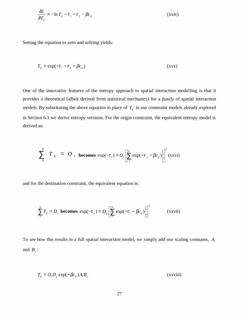
One of the innovative features of the entropy approach to spatial interaction modelling is that it
provides a theoretical (albeit derived from statistical mechanics) for a family of spatial interaction
models. By substituting the above equation in place of ijT in our constraint models already explored
in Section 6.1 we derive entropy versions. For the origin constraint, the equivalent entropy model is
derived as:
i
n
jiij OT =∑ becomes
1
)exp()exp(
−
−−=− ∑ ij
n
jjii cO βττ (xxvi)
and for the destination constraint, the equivalent equation is:
j
n
iij DT =∑ becomes
1
)exp()exp(−
−−=− ∑ ij
n
iijj cD βττ (xxvii)
To see how this results in a full spatial interaction model, we simply add our scaling constants, iA
and jB :
jiijjiij BAcDOT )exp( β−= (xxviii)

28
This represents the entropy spatial interaction model in its general form. From that equation, four
versions may be derived: origin-constrained, destination-constrained, doubly-constrained, and
unconstrained.
6.2 SPATIAL CHOICE MODELS
6.2.1 Discrete choice models
As has already been mentioned, there is little theoretical justification to support the notion that
urban systems operate in a fashion akin to Newtonian gravity. At the start of the 1970s, some
serious criticisms were levelled against gravity-type formulations of land-use–transportation
models. In reaction to this, modellers began to develop simulations that were more behaviourally
grounded. One avenue of development that was widely embraced was that of discrete choice
modelling. Broadly speaking, discrete choice models (which derive from decision theory) are
concerned with explaining phenomena in terms of decision-making. While they function in a
fashion that resembles spatial interaction models, they are actually concerned with spatial choice.
The most widely used manifestation of the discrete choice model in urban simulation is the random
utility model and variations thereof.
Random utility models proceed on a number of assumptions. The first assumption specifies that
each decision-maker is faced with a discrete set of choice alternatives—a choice is either made or
not made. The second assumes that an individual (or a group of individuals) will settle upon one
decision from a larger set of available options in such a way that the most utility, or satisfaction, is
yielded. Contextualizing this in an urban sense, we might think of a household making a location
decision amongst a set of given locations that a city has to offer so that a combination of utilities is
maximized (e.g., cost, amenities, quality of the school system, etc.). The third assumption in
random utility models is that choices are made in a probabilistic fashion—decision-makers have a
likelihood of making certain choices. Finally, it is assumed that the utility of a decision can be
divided into two components: one measuring ‘strict utility’: the fixed and measurable attributes of
utility, and the other dealing with stochastic utility: an error or disturbance term that reflects the
unobserved attributes of a given decision (Barra, 1989; Golledge and Stimson, 1997).
Mathematically, we can build up a formula for the random utility model based on these
assumptions. The notion of utility maximization can be expressed as:
29
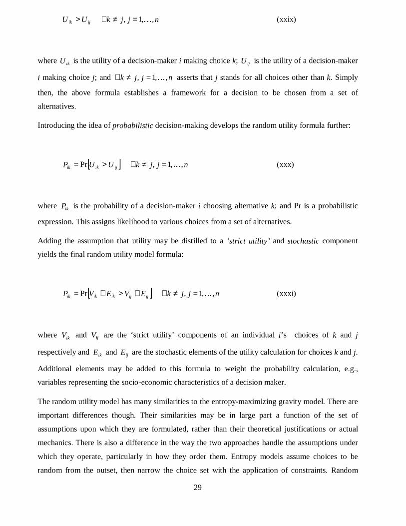
ijik UU > njjk ,,1, �=≠∀ (xxix)
where ikU is the utility of a decision-maker i making choice k; ijU is the utility of a decision-maker
i making choice j; and njjk ,,1, �=≠∀ asserts that j stands for all choices other than k. Simply
then, the above formula establishes a framework for a decision to be chosen from a set of
alternatives.
Introducing the idea of probabilistic decision-making develops the random utility formula further:
[ ]ijikik UUP >= Pr njjk ,,1, �=≠∀ (xxx)
where ikP is the probability of a decision-maker i choosing alternative k; and Pr is a probabilistic
expression. This assigns likelihood to various choices from a set of alternatives.
Adding the assumption that utility may be distilled to a ‘strict utility’ and stochastic component
yields the final random utility model formula:
[ ]ijijikikik EVEVP +>+= Pr njjk ,,1, �=≠∀ (xxxi)
where ikV and ijV are the ‘strict utility’ components of an individual i’s choices of k and j
respectively and ikE and ijE are the stochastic elements of the utility calculation for choices k and j.
Additional elements may be added to this formula to weight the probability calculation, e.g.,
variables representing the socio-economic characteristics of a decision maker.
The random utility model has many similarities to the entropy-maximizing gravity model. There are
important differences though. Their similarities may be in large part a function of the set of
assumptions upon which they are formulated, rather than their theoretical justifications or actual
mechanics. There is also a difference in the way the two approaches handle the assumptions under
which they operate, particularly in how they order them. Entropy models assume choices to be
random from the outset, then narrow the choice set with the application of constraints. Random
30
utility models, on the other hand, start out with an assumption of a rational choice base, and
introduce a random element as they proceed (Government of Ireland, 1995).
6.2.2 Non-hierarchical logit models
The most common derivative of the random utility model is the multinomial logit model. The logit
model expresses the decision choice as a function of the utility of choosing one alternative over
another. The model is derived by making assumptions regarding the random component of utility,
ijE .
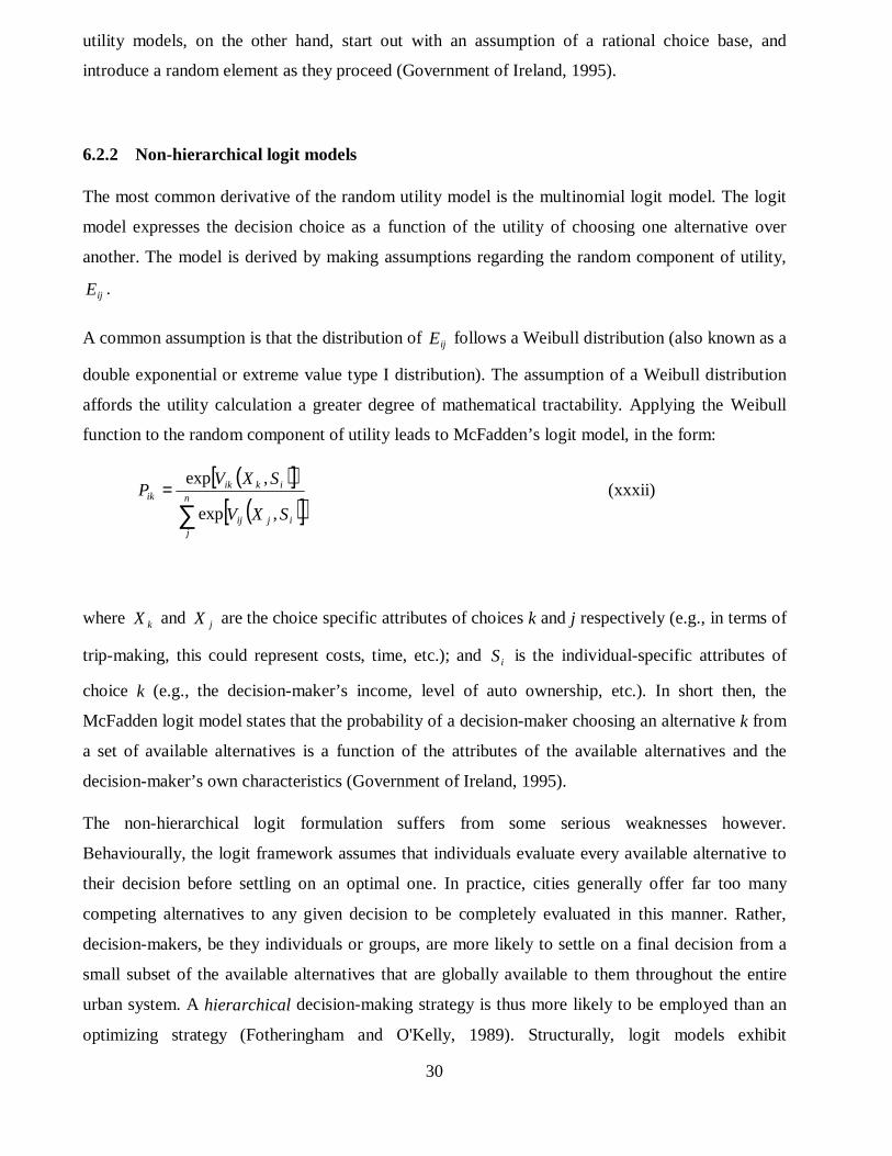
A common assumption is that the distribution of ijE follows a Weibull distribution (also known as a
double exponential or extreme value type I distribution). The assumption of a Weibull distribution
affords the utility calculation a greater degree of mathematical tractability. Applying the Weibull
function to the random component of utility leads to McFadden’s logit model, in the form:
( )[ ]( )[ ]∑
=n
jijij
ikikik
SXV
SXVP
,exp
,exp(xxxii)
where kX and jX are the choice specific attributes of choices k and j respectively (e.g., in terms of
trip-making, this could represent costs, time, etc.); and iS is the individual-specific attributes of
choice k (e.g., the decision-maker’s income, level of auto ownership, etc.). In short then, the
McFadden logit model states that the probability of a decision-maker choosing an alternative k from
a set of available alternatives is a function of the attributes of the available alternatives and the
decision-maker’s own characteristics (Government of Ireland, 1995).
The non-hierarchical logit formulation suffers from some serious weaknesses however.
Behaviourally, the logit framework assumes that individuals evaluate every available alternative to
their decision before settling on an optimal one. In practice, cities generally offer far too many
competing alternatives to any given decision to be completely evaluated in this manner. Rather,
decision-makers, be they individuals or groups, are more likely to settle on a final decision from a
small subset of the available alternatives that are globally available to them throughout the entire
urban system. A hierarchical decision-making strategy is thus more likely to be employed than an
optimizing strategy (Fotheringham and O'Kelly, 1989). Structurally, logit models exhibit

31
weaknesses owing to the independence from irrelevant alternatives problem and the assumption of
regularity. The problem of independence from irrelevant alternatives (popularly known in transport
modelling as the ‘red-bus-blue-bus conundrum’) lies in the fact that logit models assume that the
ratio of probabilities of an individual selecting two alternatives is irrelevant from the addition of an
extra alternative. Yet, the introduction of additional alternatives is generally quite relevant in spatial
terms. Closely related to this is the idea of regularity, which refers to the notion that within the logit
framework it is not possible to change the probability of selecting an alternative by adding another
alternative to the choice set (Fotheringham and O'Kelly, 1989). In the context of an urban system
this assumption holds little value; it leaves the decision-making process unaffected by any offer of
additional choices to a decision-maker.
6.2.3 Nested logit models
The nested logit model departs from the basic logit formulation by introducing hierarchy into the
decision-making process. Nested models assume that decision-makers process information about
choices in a chained fashion and that the modeller is aware of the form of that chain. In this sense
they attempt to circumvent the weaknesses of the non-hierarchical model by assuming that decision
makers make choices sequentially, rather than wading through every available option at once.
A common application of the nested model is to travel choice. Various sequential stages in the
decision to travel can be identified, e.g., whether or not to make a trip; where to go; by what mode a
trip should be made; and on what route to travel. This method of simulation abstracts from
irrelevant (or less relevant) information regarding the decision, and focuses the choice on the set of
alternatives that are most applicable. Mathematically, this results in a set of conditional probabilities
for each of the sequential stages in the decision-making process. Aggregating these probabilities
yields the likelihood of a choice being made such that:
( ) ( ) ( ) ( ) ( )cbadPbacPabPaPdcbaP ,,|,||... = (xxxiii)
where a, b, c, and d refer to the four sequential stages in the decision hierarchy (e.g., whether to
travel, destination, mode, and route). It is important that the estimation process begin with the last

32
step in the hierarchy and work its way back to the beginning in order to ensure that the strict utilities
are preserved throughout the process (Government of Ireland, 1995).
Formulating the nested model in spatial terms, decision-makers can be regarded as choosing options
from a set of clusters. Continuing with our trip-making analogy, we now have individual trip-
makers (or perhaps groups of trip-makers) who make decisions about their trips but also have to
consider a range of spatial options in which to focus those choices. Mathematically, this can be
represented as:
( ) ( )
( ) ( )∑ ∑
∑
=
∈
∈
n
s
n
skikis
n
skikis
is
VV
VV
P σ
σ
expexp
expexp
(xxxiv)
where isP is the probability that a decision-maker i will select a particular spatial cluster s to focus
its decision in; ( )∑∈
n
skikVexp is termed an ‘inclusive value’ and describes the attractiveness of a
cluster as a function of the individual alternatives available within that cluster (Fotheringham and
O'Kelly, 1989); and σ represents the extent to which decision-makers process their information
hierarchically, and ranges in value from zero to one, with 1=σ denoting decision-makers who do
not process their information hierarchically at all.
Once a decision-maker has selected a given spatial cluster, s, to narrow her choice set, all that
remains is for an option (or alternative), k, to be settled upon. The likelihood of a decision-
maker selecting a particular alternative k, within the selected spatial cluster s, is then calculated as:
( )( )∑
∈
∈ =n
skik
iksik
V
VP
exp
exp sk ∈∀ (xxxv)
and the probability of a decision-maker selecting k from the set of all alternatives is:

33
sikisik PPP ∈= (xxxvi)
Spatial choice models are perhaps more appropriate representations of how land-use and
transportation systems organize than spatial interaction models, but they suffer from weaknesses.
Notably, it is widely understood that the distinctions between choice categories may often be fuzzy
rather than discrete. Spatial choice models do not commonly accommodate this.
6.3 BID-RENT THEORY
Figure 6. Diagram illustrating land use patterns distributed spatially across a theoretical city
according to bid-rent theory
The final modelling technique, which along with spatial interaction and spatial choice, underlie the
most common land-use–transportation models is bid-rent theory. Bid-rent theory (popularized by
Alonso) owes a great deal to the von Thunen model that we explored in Section 4, as Figure 6
illustrates. Proceeding from a set of simplifying assumptions (notably, monocentric cities and a
limited range of land uses), bid-rent theory offers an explanation of the spatial distribution of urban
activities. The central argument of bid-rent theory is that land uses will organize geographically
based on their capacity to compete for land rents. That capacity to compete is controlled by the
34
value, profit, or utility that an activity places on accessibility to a central urban core. Given these
considerations, land uses will tend towards a spatial arrangement akin to that illustrated in Figure
6—with businesses located close to the urban core and industry and residences situated towards the
urban periphery.
While the notion of bid-rents has enjoyed a wide application in urban modelling, and has a limited
theoretical justification, the theory does not easily transfer to practice. The utility function, in
particular, can be difficult to calculate. Often, it involves a monetary component (e.g., travel time
and/or travel cost related to distance from work). But in many circumstances the utility function
also contains non-monetary conditions that are difficult to cost—the availability of space, fresh air,
peace and quiet; location prestige; neighbours; family ties; etc. (Balchin and Kieve, 1977).
Nevertheless, bid-rent theory enjoys a pivotal position in many operational land-use–transportation
models and is an important ingredient in their formulation.
A variant of bid-rent models—hedonic price models—has gone further towards operationalizing
some of the factors that weigh into the bid-rent calculation. Hedonic price models distil real estate
values into constituent components (e.g., land value, structure value, number of bedrooms in
property, proximity to schools, etc.), each of which has an associated value. Often these models can
be incredibly disaggregated. However, they are weakened to some extent by their reliance on price
as a framework for formulating ideas about the dynamics of urban systems. Also, because of
privacy concerns, price data can be difficult to obtain, especially data spanning multiple time
periods. Moreover, many things are difficult to price.
7 INDIVIDUAL MODEL COMPONENTS (SUB-MODELS)
With a grounding in the important modelling principles common to land-use–transportation models
behind us, the discussion now moves onto a treatment of the various sub-models that make up land-
use–transportation models. In Section 7.1 simulation of the land use system will be described in
terms of location, development, and equilibrium; then the focus will shift in Section 7.2 to a
representation of the transport system, discussed in terms of potential demand modelling and trip
generation, trip distribution, modal split, trip assignment, accessibility, and the generalized costs of
travel. Ways of integrating the land-use and transport systems in a simulation are then mentioned in
Section 7.3, as are the introduction of policy elements to the modelling framework in Section 7.4.

35
7.1 THE LAND USE SYSTEM
The essential components of the land use system, in terms of land-use–transportation modelling, are
location and development.
7.1.1 Location
The urban land use system is largely modelled by simulating the mechanisms that affect the spatial
location of urban activities in a city. The most important of these location factors for simulation
purposes—accessibility—will be discussed in more detail in later sections. A number of other
important geo-economic concepts underpin land-use–transportation models, serving as proxies for
the complex interactions and motivations driving urban location. Among these are the ideas of bid-
rent, travel costs, inertia (stability in the occupation of land), topography, climate, planning, and
size.
As the discussion surrounding bid-rent theory alluded to, not all land uses in the city have the same
location considerations. It is useful, therefore, within a land-use–transportation model, to
decompose the location decision to represent a broad classification of the most important land uses
in a city. Residential location and firm location are essential considerations, and occasionally
industrial location is modelled.
7.1.1.1 Residential location
There are three main theories explaining the rationales underlying urban residential location: bid-
rent theory, travel cost minimization theory, and travel cost and housing cost trade-off theory.
Expressing the household location decisions of two households in a monocentric city in a bid-rent
framework generates bid-rent curves such as those displayed in Figure 7.

36
Figure 7. Diagram illustrating a residential bid-rent curve for a monocentric city.
When seeking out a location (in this conceptual, economic sense), each household pursues a
location on the bid-rent curve where the land price curve touches the bid-rent-curve nearest the
origin, i.e., a household seeks the location that yields the greatest utility at current market rents
(Harvey, 1996). The shape of a household’s bid-rent curve is dependent upon their particular
situation (tastes, income, etc.). For example, a young family (household B) will generally require
space and access to schools. Its bid-rent curve is likely to be relatively flat as a result (implying that
a household is more likely to locate in the suburbs). On the other hand, single people, the elderly, or
families consisting mainly of wage earners (household A), are likely to have steeper bid-rent curves,
and may favour locations closer to the CBD.
Travel cost minimization theory assumes that the only consideration in the residential location
decision is that households select locations that reduce their need to travel. If we consider a city
with jobs located in a central core, this implies that the most sought after locations would be close
to the CBD, while the less popular areas would be concentrated on the urban fringe. Socio-
economically, this would suggest concentrations of wealthy households in the central city, with
poorer households towards the urban periphery. In reality, the cost of travel is not the only
residential location factor affecting the decisions of households; factors such as open space and
quality of housing muddy the issue and the opposite is generally true: the poor end up closer to the
CBD and the rich live farther out. Also, jobs are increasingly located in the suburbs. Nevertheless,
travel cost minimization theory does have some relevance to household location (particularly
through the notion of accessibility).

37
Travel cost and housing cost trade-off theory assume that households trade off the competing
influence of housing cost and travel cost in making their residential location decision. This implies,
in geographic terms, that land values will be higher close to a central business district and lower
towards the periphery. While this is largely true in practice, there are many complicating factors,
both economic and non-economic. High-income households may not have to trade off housing cost
against travel cost, because they may be able to afford both. People who can afford to live close to
the CBD may elect not to because they wish to enjoy the amenities on offer in the suburbs (e.g.,
environment, space, and for reasons of segregation). Because of the dearth of available space in
central cities, outer areas generally offer a wider range of opportunities for the construction of new
and expensive houses. Also, transportation innovations may make outer locations more accessible
to a CBD than inner suburban areas. This is significant; jobs are increasingly relocating to
peripheral sites. Additionally, location decisions may be heavily reliant on the availability of
income and mortgage finance, which is often distributed aspatially within a given metropolitan area.
And there may be a time lag before households react to changes in housing costs.
There are also many non-economic reasons that play equally important roles in affecting household
location decisions. For example, some households may have a low degree of mobility in their
decision to move. There may also be more pressing familial reasons why a household seeks to
move, and governing the type of real estate they may demand, e.g., changes in employment,
marriage, family size, and age.
7.1.1.2 Business location
Figure 8. Diagram illustrating a business bid-rent curve for a monocentric city.

38
Households may desire central areas as much as other urban land uses, but they can rarely hope to
outbid uses such as industry and business (unless the residences compose multi-storey blocks of
residential units) because they cannot derive as much profit (or utility) as those other uses. In terms
of bid-rent, firms generally out-bid all other activities in the urban location decision, simply because
they can derive the most profit from occupying a particular site. In this sense, they tend to have the
steepest bid-rent curves (Figure 6). We find that firms tend to locate where the land price curve
touches the bid-rent curve. At that point, the most profitable location at current market rents is
realised, which is often in, or close to, the CBD. However, firms requiring large sites may have a
flatter bid-rent curve (firm B), and may locate in suburban areas or towards the urban periphery
(Figure 8).
7.1.1.3 Industrial location
Industrial land uses have the same need for proximity to central sites as do firms. Their location
motivation is also similar to that of firms: availability of labour, access to transportation, auxiliary
services, etc. However, their need for central locations is not as great. As a result, industries are not
as well equipped to compete for central sites and their rent gradients tend to be flatter than those of
commercial firms.
In recent years there have been significant changes in the location behaviour of most urban land-
uses because of advances in the provision of transport infrastructure, changing socio-demographics
amongst urban populations, and alterations in the spatial structure of the city. While these
reorganizations have affected all urban land uses, the impact of these changes has been particularly
profound for manufacturing industry and its location within metropolitan areas. Manufacturing uses
have been persuaded or forced out of central locations largely because of developments in the
provision of roadways—the contemporary wave of road building has focused mainly in outer urban
areas. Nevertheless, a large degree of inertia remains for centrally located manufacturing industry,
fuelled by traditional preferences for downtown sites and the benefits of external economies of
agglomeration in central areas.
7.1.1.4 Simulating location via the Lowry framework
One way of handling the idea of location in a simulation sense is via the Lowry framework.
Conceived of in his Model of Metropolis (1964), the framework proceeds on the premise that the

39
place of employment governs the place of residence—jobs decide where people live. In the Lowry
framework, employment is divided into basic (mainly manufacturing) and non-basic (mainly
service) sectors. The framework takes basic employment (which must be exogenously supplied)
together with endogenously derived service employment and uses them to estimate the location of
residents. This estimate of residential location is then fed back into the model to predict the location
of service employment. The model then proceeds iteratively through these steps, assigning activities
to urban locations.
Lowry’s assumption that basic industry should be exogenously determined (outside the model) was
based on his observations that basic industry has specialized site requirements and external markets,
and that its location decisions are independent of the residential population (Oryani and Harris,
1996). However, Lowry suggested that service employment be endogenously derived (within the
model) since its location decisions are closely related to residential demand. He also assumed that
the residential location decision was made in relation to both combined service and basic
employment.
Distilling the Lowry framework to its two principal mechanisms—residential and firm location—
presents a clearer idea of how the model operates. In the residential component, population (or
households) are assigned to residential locations in origin zones based on their places of
employment in destination zones. Two main factors are used to govern this location assignment
process: zonal attractiveness and distance. For households, zonal attractiveness can be characterized
by variables such as floor space; housing prices or rents; availability of schools, shops, health
services, leisure and recreation facilities, etc. The other factor—distance between places of
residence and work—may be considered in physical terms or as the cost of traversing that distance
in monetary costs or time expenditure.
In the service employment (firm) component, firm location is directly linked to residential location,
implying that service employment is located either alongside, or soon after, residences. The major
factors driving service employment are governed to be accessibility to consumers and rental costs
for work sites.
The Lowry model is expressed mathematically as a series of singly constrained spatial interaction
models. It proceeds sequentially and iteratively through four main stages. In the first step, basic and
service employment totals are combined and this figure is used to estimate total employment in a
destination zone. (Service employment totals are usually set to zero in the first iteration.)
Mathematically this takes the form:

40
sj
bjj EEE += (xxxvii)
where Ej is an estimate of total employment in destination zone j; bjE is an estimate of basic
employment in zone j; and sjE is an estimate of service employment in zone j.
The employment estimate value (Ej) is fed into another equation in the second stage to estimate how
residents should be allocated to an origin zone i:
( )ijr
ijjij cWBER βµ α −= exp (xxxviii)
where ijR is the estimated number of residents that live in origin i and work in destination j; jE is
an estimate of total employment in destination zone j (supplied by the first stage); µ is a population-
to-employment ratio; jB is a parameter that ensures that the correct number of residents is allocated
to zone i, i.e., that µjiji ER = ; αiW is the attractiveness of zone i (e.g., in terms of floor space for
residents); rβ regulates the effect of transport costs on the distribution of residents; and ijc is the
cost of travel from i to j.
In the third stage, service employment is allocated to destination zones j based on places of
residence in zones i (calculated in the previous step):
( )ijs
jiisij cWsARE βα −= exp (xxxix)
where sijE is an estimate of the number of service workers living in zone i and working in
destination zone j; iR is the number of residents in origin zone i; s is a service employment-to-
population ratio; iA ensures that the correct number of service employees is allocated to zone j, i.e.,
that sRE isijj = ; and where ( )ij
sjji cWA βα −= exp .
In the fourth stage, calculation then passes back to the first step. Here, service employment is added
back to exogenous basic employment. At each subsequent iteration, a number of residents and

41
service employees are added to the calculation, but this number grows progressively smaller with
each iteration, eventually converging to zero.
The basic framework can be extended to add realism to the model. For example, service
employment may be disaggregated within the model to accommodate a variety of services (e.g.,
retailing, education, healthcare, etc.).
7.1.2 The land development process
Another important component of the generic land-use–transportation model, along with location, is
the simulation of land development (although many models overlook this component). In
theoretical terms, a need to increase the available supply of land in a given urban area is prompted
by excess demand for urban real estate. Developers will develop a site if they judge that they can
turn a profit. A number of factors weigh in on this profit calculation, however. Developers calculate
profit margins; these are a function of the trade-off between input costs (the costs of developing a
site) and the expected selling price of the development. The actual acquisition price of the site for
development is normally valued by the residual method of valuation. If a developer is able to
acquire a site for a price below its residual value, she or he can (potentially) turn a profit by
developing that site. The residual value may be calculated according to the following equation:
PCMV −−= (xl)
where: V refers to the residual value of a development site (often expressed per annum), M refers
to the market value of the finished product, C refers to the full costs of development, and P refers
to the developer’s required profit on gross development value (Adams, 1994).
There may be a range of input costs associated with land development, including expenses such as
land, labour, materials, fixed costs, marketing, the costs of capital, fees, and interest charges
(Adams, 1994; Bramley et al., 1995). (Interest charges strongly influence development on the
supply side—if interest charges go up, the cost of borrowing capital for development rises.)
However, the determination of a profit calculation is further complicated by the issue of the timing
of land acquisition in relation to the sale of the development as this impacts upon the cost of the
land and the turnover time of capital (Bramley et al., 1995).

42
7.1.2.1 Land banking
All developers will land bank (withhold land from development) to a certain degree. Land will
generally need to be held from development for a minimum of two years, simply for operational
reasons (Bramley et al., 1995). However, many developers (as well as landowners) may withhold
land from development for speculative reasons if they think that the profits to be gleaned from the
future sale price of the land can at least offset their costs in holding the land over the duration of the
development. Money invested in development is essentially dead money until it is recouped at the
time of sale. If the money used to develop a site has been borrowed, it is a liability over the time of
the development. The capital that would have been realised from the development and sale of a tract
of land could alternatively be invested by other means, potentially generating a profit over the entire
development period (which, in many cases, spans several years). Additionally, a developer must
also bear in mind the cost of property taxes that may need to be paid on the land over the timeline of
the development. The considerations influencing the decision to hold land speculatively from
development may be thus generalized in the following functional relationship:
( )Pgnsrriifto ,,,,,,, **= (xli)
where to is the optimum time period for holding land from development for speculative reasons; i is
the individual investor’s interest rate (which varies amongst individuals depending on their ability
and capacity to invest, and the quantity and quality of their investment opportunities); i* is the
discounted expected percentage return on an alternative investment; r is the net rate of return on the
land; r* is the discounted expected percentage return on the land (which should include a risk
premium); s is the marginal personal income tax rate assessed to the landowner; n is the number of
years in the speculator’s time horizon (depending on their forecast of land demand); g is a
subjective discount factor reflecting risk; and P is a property tax (Bahl, 1968).
In terms of operationalizing these sorts of functional relationships into a simulative framework
within land-use–transportation models, traditional efforts have been weak (if existent at all).
Supply-side modelling (development and redevelopment) is, in many cases, simply absent from
simulative frameworks (notable exceptions include UrbanSim, under development at the University
of Washington (Waddell 1998a; 1998b).

43
7.1.3 Supply, demand, and equilibrium
Because land-use–transportation models are overwhelmingly rooted in urban economic theories
about how urban systems work, much of their mechanics is phrased econometrically. On the
broadest economic level, urban land use manifests itself spatially through a complex trade-off
between supply, demand, and equilibrium. Because the supply of and demand for land are generally
in a state of disequilibrium, there is usually a scarcity or excess of land available for different uses
within the city at any given time.
7.1.3.1 Urban land supply
The total supply of land in any given urban area can generally be regarded as being largely fixed (or
inelastic)—for the most part, new land cannot be readily created or destroyed. Of course, there are
exceptions: land may be gained or forfeited through territorial acquisitions or losses, or through
land reclamation or destruction. Additionally, land may be brought into supply as urban areas
expand beyond their peripheries and encroach upon agricultural hinterlands. While the total supply
of land is largely static, the available supply of land at any one time is dynamic due to factors such
as intensity of use, planning policies that might permit or deny development, physical constraints,
improvements in building technology, and the behavioural choices of landowners who might
withhold land from development for various reasons.
7.1.3.2 The demand for urban land
The demand for land in a city is a function of the conceived profitability or utility of its use by
existing or potential users. Because of the relatively fixed nature of urban land supply, it reacts quite
slowly to increases or decreases in demand. Therefore, it is demand that is the real determinant of
urban land prices.
Demand itself is really determined by two factors: use value and exchange or sale value (Kivell,
1993). The use value of urban land refers to the demand that it generates from users who wish to
actually utilize the land for some purpose. Essentially, use value is derived from the functional use
of the land, e.g., as a business or a site for the manufacture of certain goods. Exchange value derives
from the sale of land at a profit to another user. Additionally, there are other factors that influence
the demand for urban land, including interest rates, allowances for risk, and expectations of capital
gain.
44
7.1.3.3 Reconciling supply and demand through the urban land market
The forces of supply and demand come together in the urban land market. Ideally, at any given
time, the competition between land supply and demand would reach a state of equilibrium in which
a balance was struck between the two. In a perfectly competitive market, rapid shifts in price would
balance the demand for land with the quantity supplied. Such markets would eliminate surpluses
and overcome shortages quickly (Adams, 1994). However, the urban land market is anything but
ideal, and generally tends towards a state of disequilibrium at any moment. This tendency towards
disequilibrium (or lagged response of supply to demand) is the result of several inefficiencies in the
urban land market. These include the imperfect knowledge of buyers and sellers; the betrayal of
conditions of perfect competition (because property is often dominated by few buyers and sellers);
the uniqueness of supply (in terms of quality, age, configuration, and location); barriers to ease of
entry and exit of buyers and sellers to the market such as high transaction costs; infrequent
transactions—land and property are bulky goods, acquired infrequently; externalities (costs of
benefits arising from an activity that do not accrue to the person or group engaging in the activity);
geographical inertia; the immobility of land; time-absorption in the development of land; the
influences of conservation policies; the monopoly power of some agencies such as planning
authorities, property companies, and mortgage institutions; and the role of non-monetary factors
such as sentiment, symbolism, and pride of ownership (Adams, 1994; Balchin and Kieve, 1977;
Kivell, 1993).
7.1.3.4 Modelling equilibrium using constraints
As previously mentioned in Section 6, the application of constraints to basic models serves as a
proxy for equilibrium in the generic land-use–transportation model. Of course, the theoretical
justification for this is weak. The very notion of equilibria in urban systems is debatable.
Additionally, the introduction of constraints is likely to be a result of inadequacies in the behaviour
of the model, rather than a theoretical foundation. Nevertheless, the constraint does serve as a vague
mechanism for reconciling demand and supply within the model.
Other, more theoretically justified methods of reconciling demand and supply in land-use–
transportation include the notion of market clearing. In a simulative framework that incorporates
price information (land prices, rents, etc.), market clearing is represented by adjusting prices to

45
balance the demand for space (generated by competing uses) with the supply of space in the urban
system2.
7.2 THE TRANSPORT SYSTEM
The second major component of a land-use–transportation model, simulated alongside land-use, is
the transport system. The traditional way of characterizing the transportation system in urban
simulation models is a four-stage process. This process begins with modelling travel demand and
generating an estimate of the amount of trips expected in the urban system. The second phase, trip
distribution, allocates the trips generated in origin zones to destinations in the urban area. The third
phase is modal split. Here trips are apportioned to various modes of transport (e.g., by automobile
or public transportation). The four-stage simulation process concludes with a trip assignment
module that takes estimated trips that have been generated, distributed, and sorted by mode, and
loads them onto various segments of the transport network. Transport simulation usually proceeds
sequentially amongst these four stages in the order in which they are described above (Figure 10).
Figure 10. Diagram illustrating the four-step modelling process for transport.
2 For a description of a market-clearing mechanism used in an operational model, see Waddell, 1998a, 1998b.

46
7.2.1 Potential demand modelling and trip generation
Potential travel demand (an estimate of the volume of trips likely to be made in a given urban area
and time) can be derived for both journey-to-work trips, trips for other purposes (e.g., leisure, or
shopping), or aggregated as a total measure of trips for all purposes.
Demand for journey-to-work trips can be derived from location models at the land use level using
figures for residential occupation:
ijwij RQ = (xlii)
where wijQ is the potential demand for work trips between an origin and destination (from i to j) and
ijR is the number of residents that live in i and work in j, i.e., the population that drives the demand.
Demand for trips for other purposes is derived from an origin-constrained spatial choice model:
( ) ( )nij
nnjii
nij cWARQ βα
−= exp (xliii)
where nijQ is potential demand for non-work-related trips from i to j for each purpose n (e.g., for
shopping or leisure); iR is the number of residents living in origin zone i; iA is a balancing factor
that ensures that the simulated iR is equal to an exogenously-determined iR , and where
( ) ( ) 1exp
−−= n
ijnn
jji cWA βα; n
jW is the attractiveness of destination zone j for activity n (e.g., the
floor space occupied by shops); and nijc is the composite cost of travel from zone i to zone j.
Combining these two demand functions, we can estimate total demand for all trips across all
purposes by adding potential demand for non-work-related trips over activity n to potential demand
for work-related trips:
wij
nijnij QQQ += (xliv)
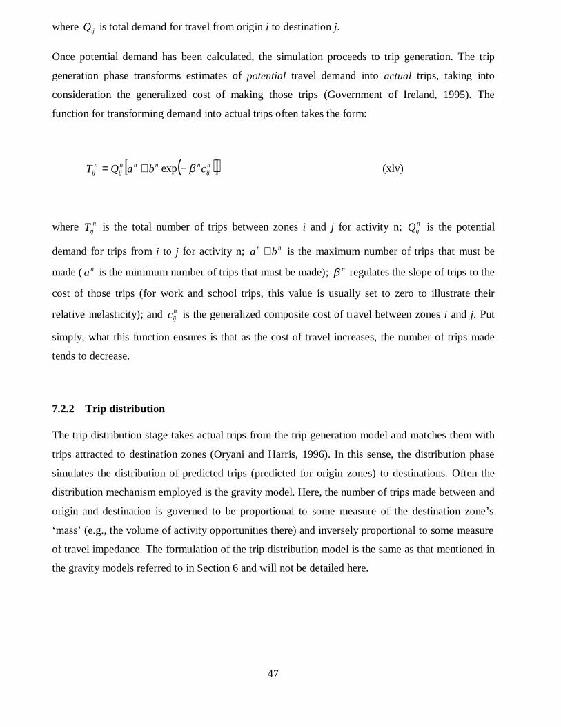
47
where ijQ is total demand for travel from origin i to destination j.
Once potential demand has been calculated, the simulation proceeds to trip generation. The trip
generation phase transforms estimates of potential travel demand into actual trips, taking into
consideration the generalized cost of making those trips (Government of Ireland, 1995). The
function for transforming demand into actual trips often takes the form:
( )[ ]nij
nnnnij
nij cbaQT β−+= exp (xlv)
where nijT is the total number of trips between zones i and j for activity n; n
ijQ is the potential
demand for trips from i to j for activity n; nn ba + is the maximum number of trips that must be
made ( na is the minimum number of trips that must be made); nβ regulates the slope of trips to the
cost of those trips (for work and school trips, this value is usually set to zero to illustrate their
relative inelasticity); and nijc is the generalized composite cost of travel between zones i and j. Put
simply, what this function ensures is that as the cost of travel increases, the number of trips made
tends to decrease.
7.2.2 Trip distribution
The trip distribution stage takes actual trips from the trip generation model and matches them with
trips attracted to destination zones (Oryani and Harris, 1996). In this sense, the distribution phase
simulates the distribution of predicted trips (predicted for origin zones) to destinations. Often the
distribution mechanism employed is the gravity model. Here, the number of trips made between and
origin and destination is governed to be proportional to some measure of the destination zone’s
‘mass’ (e.g., the volume of activity opportunities there) and inversely proportional to some measure
of travel impedance. The formulation of the trip distribution model is the same as that mentioned in
the gravity models referred to in Section 6 and will not be detailed here.

48
7.2.3 Modal split
The modal split sub-model is concerned with estimating what proportion of trips is made by each
defined mode of travel from an origin to a destination zone. In mathematical terms, this is most
commonly expressed as a multinomial logit model. The logit model represents the mode choice as a
function of the disutility or cost of using one mode of travel (e.g., private automobile) over another
(e.g., public transit). Often the logit model may be specified hierarchically to circumvent the ‘red
bus-blue bus’ conundrum. The non-hierarchical logit model will generally take the form:
( )( )∑ −
−=
n
k
nkij
n
nkij
n
nij
nkij
c
cTT
β
β
exp
exp(xlvi)
where nkijT is the number of trips between i and j by mode k for activity n; n
ijT is the total number of
trips between i and j for activity n; and ( )
( )∑ −
−n
kc
nkij
n
nkij
n
c
β
β
exp
exp is the share of trips made by each mode k
between i and j for activity n.
7.2.4 Trip assignment (route choice)
The trip assignment or route choice phase takes estimated trips, already sorted by mode, and assigns
them to routes on the transport network. Again, the technique used to express this mathematically is
usually by means of a multinomial logit model (although with capacity constraints added). This
may generally take the form:
( )( )nkp
ijn
p
nkpij
n
nkij
nkpij
c
cTT
ββ
−−
=exp
exp(xlvii)
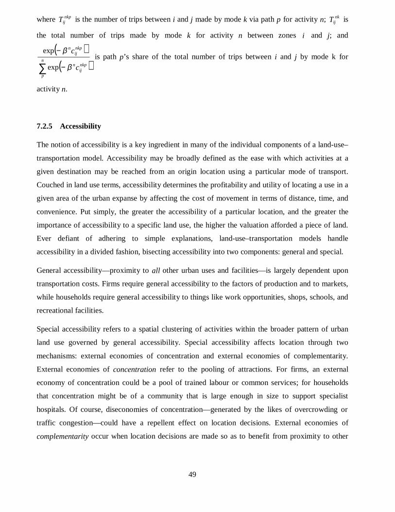
49
where nkpijT is the number of trips between i and j made by mode k via path p for activity n; nk
ijT is
the total number of trips made by mode k for activity n between zones i and j; and
( )( )∑ −
−n
p
nkpij
n
nkpij
n
c
c
β
β
exp
exp is path p’s share of the total number of trips between i and j by mode k for
activity n.
7.2.5 Accessibility
The notion of accessibility is a key ingredient in many of the individual components of a land-use–
transportation model. Accessibility may be broadly defined as the ease with which activities at a
given destination may be reached from an origin location using a particular mode of transport.
Couched in land use terms, accessibility determines the profitability and utility of locating a use in a
given area of the urban expanse by affecting the cost of movement in terms of distance, time, and
convenience. Put simply, the greater the accessibility of a particular location, and the greater the
importance of accessibility to a specific land use, the higher the valuation afforded a piece of land.
Ever defiant of adhering to simple explanations, land-use–transportation models handle
accessibility in a divided fashion, bisecting accessibility into two components: general and special.
General accessibility—proximity to all other urban uses and facilities—is largely dependent upon
transportation costs. Firms require general accessibility to the factors of production and to markets,
while households require general accessibility to things like work opportunities, shops, schools, and
recreational facilities.
Special accessibility refers to a spatial clustering of activities within the broader pattern of urban
land use governed by general accessibility. Special accessibility affects location through two
mechanisms: external economies of concentration and external economies of complementarity.
External economies of concentration refer to the pooling of attractions. For firms, an external
economy of concentration could be a pool of trained labour or common services; for households
that concentration might be of a community that is large enough in size to support specialist
hospitals. Of course, diseconomies of concentration—generated by the likes of overcrowding or
traffic congestion—could have a repellent effect on location decisions. External economies of
complementarity occur when location decisions are made so as to benefit from proximity to other

50
uses or activities. For example, smaller shops situating themselves parasitically beside dominant
retailers, or households locating near to parks (Balchin and Kieve, 1977).
Mathematically, there exist a diversity of mechanisms for describing accessibility. The basic format
for measuring accessibility is as a function of opportunities in a destination zone and the cost of
travel between an origin and that destination—accessibility as a function of the attraction of the
destination and the ease of reaching it. One of the simpler expressions of this kind is the summation
of spatial separation:
∑=
=n
jiji dA
1
(xlviii)
where iA is a measure of the accessibility of an origin zone i, and ∑=
n
jijd
1
represents the distance
between origin zone i and destination zone j, summed across all destination zones j (Lee and
Goulias, 1997).
The above measure may be more closely fitted to a city by including some form of distance
decay parameter, reflecting the notion that people are less inclined to make longer journeys. There
are a number of ways in which distance decay can be added to the basic summation formula above.
The parameter may be added as a constant in the form:
kn
jiji dA
−
=∑=
1
(xlix)
where k− represents the effect of distance decay on the accessibility of an origin zone (Lee and
Goulias, 1997). Alternatively, a negative exponential function could be applied to the basic formula
to describe a more realistic form of distance decay:
( )∑=
−=n
jiji dA
1
exp β (l)

51
where β− now represents distance decay (in a negative exponential form). There are some
complications with the negative exponential expression, however. Its main failing is that it
describes distance-decay as a rapid drop in accessibility with distance from a centre. One way to
circumscribe this flaw is to describe distance-decay as a Gaussian function. The Gaussian function
has the advantage of offering a smoother characterization of distance-decay, more akin to real-
world patterns. The Gaussian description of distance-decay represents accessibility decline initially
as a slow abatement from an origin i, with a smooth tapering to zero as distance from that origin
increases:
∑=
−=
n
j
ij
i v
dA
1
2
exp , with 22 •= dv (li)
or, rewriting the equation with all terms included we get:
( )∑= •
−
=
n
j
ij
i d
dA
1
2exp (lii)
where v is a constant, and 2•d is the square of the distance from origin i at which accessibility is
deemed to decline at the most rapid rate (Lee and Goulias, 1997).
Other ways of expressing accessibility mathematically include measures based on gravity
formulations, and isochrones. As we have seen, gravity-type accessibility measures introduce a
weight representing the ‘mass’ of opportunities at a destination zone and incorporate some indicator
of the cost of travel between origin and destination:
∑=
=n
jijji cOA
1
(liii)
where jO corresponds to the mass of opportunities at destination zone j, and ijc represents the costs
of travel between origin i and destination j.
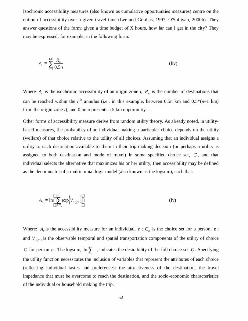
52
Isochronic accessibility measures (also known as cumulative opportunities measures) centre on the
notion of accessibility over a given travel time (Lee and Goulias, 1997; O'Sullivan, 2000b). They
answer questions of the form: given a time budget of X hours, how far can I get in the city? They
may be expressed, for example, in the following form:
∑=
=0,1
1 5.0n
ni
n
RA (liv)
Where iA is the isochronic accessibility of an origin zone i, nR is the number of destinations that
can be reached within the nth annulus (i.e., in this example, between 0.5n km and 0.5*(n–1 km)
from the origin zone i), and 0.5n represents a 5 km opportunity.
Other forms of accessibility measure derive from random utility theory. As already noted, in utility-
based measures, the probability of an individual making a particular choice depends on the utility
(welfare) of that choice relative to the utility of all choices. Assuming that an individual assigns a
utility to each destination available to them in their trip-making decision (or perhaps a utility is
assigned to both destination and mode of travel) in some specified choice set, C , and that
individual selects the alternative that maximizes his or her utility, then accessibility may be defined
as the denominator of a multinomial logit model (also known as the logsum), such that:
( )( )A Vn n CC
n
n
=
∀∈∑ln exp (lv)
Where: An is the accessibility measure for an individual, n ; Cn is the choice set for a person, n ;
and ( )Vn C is the observable temporal and spatial transportation components of the utility of choice
C for person n . The logsum, ln∑ , indicates the desirability of the full choice set C . Specifying
the utility function necessitates the inclusion of variables that represent the attributes of each choice
(reflecting individual tastes and preferences: the attractiveness of the destination, the travel
impedance that must be overcome to reach the destination, and the socio-economic characteristics
of the individual or household making the trip.

53
7.2.6 Generalized costs of travel
An important component of location decisions (and indeed of many of the calculations we have
already reviewed) is the idea of travel cost. There are three main ways in which the costs of travel
are considered in land-use–transportation models: travel time, composite costs of travel, and
changes in consumer surplus.
Travel time on a particular path (a proxy for travel cost) is a function of the ratio of path volume to
path capacity (the amount of traffic on a road versus the amount a road can handle).
Mathematically, this is expressed as:
+=
η
αmax
0 1Q
QTTQ (lvi)
where QT is travel time at a given traffic flow Q ; α is a parameter to be estimated by the model;
Q is the traffic flow expressed as vehicles per hour; and maxQ is the practical capacity of the route.
The composite costs of travel between zones i and j by a transport mode k can be derived by
aggregating nkpijc (the cost of travel between i and j for activity n, by transport mode k, along path p)
over all paths p (the subscript p denoting aggregation over all paths):
( )
−= ∑
n
p
nkpij
n
n
nkij cc β
βexpln
1(lvii)
where nkijc is the composite cost of travel between zones i and j by mode k for activity n; nβ
regulates the slope of trips to their cost (this value is usually set to zero for work and school trips,
reflecting their general inelasticity); and nkpijc is the composite cost of travel between zones i and j
by mode k over path p for activity n.
Similarly, the composite costs of travel between zones i and j can be obtained by aggregating nijc
over all modes k (the subscript k denoting aggregation over all modes k):

54
( )
−= ∑
n
k
nkij
n
n
nij cc β
βexpln
1(lviii)
where nijc is the composite cost of travel between i and j for activity n; and nk
ijc is the composite cost
of travel between i and j by mode k for activity n.
Changes in consumer surplus can be derived at both the route choice and the mode choice level.
However, to avoid double counting in models, usually only consumer surplus at mode choice level
needs to be evaluated. Again, this calculation is performed mathematically as:
( )
( )
−
−−=∆
∑
∑n
k
nkij
nnkij
n
k
nkij
nnkij
n
cT
cTW
)1(exp
)2(expln
1
β
β
β(lix)
where W∆ is the change in consumer surplus; (2) is the scenario being evaluated, and (1) is the
base case against which scenario (2) is being evaluated.
7.3 INTEGRATING LAND USE AND TRANSPORTATION
In previous modelling efforts, land use variables were treated as being exogenous to the transport
system. However, in recognition of the interdependence of land-use and transportation, there have
been recent attempts to link land-use models to transport models in an integrated fashion. In such
cases there is an explicit treatment of the connective feedbacks linking the two systems.
There are two main ways of linking land-use and transport models. The first is via an instantaneous
link at the trip distribution stage of the model. Here, the land use system provides the transport
system with estimates of the location and volume of potential trips. The second is through a time-
lagged link to the activity location stage of the model via the notion of accessibility. At this level,
accessibility affects travel costs, which in turn impacts upon urban activity location. The inclusion
of these feedback mechanisms in integrated models marks an innovative departure from

55
conventional four-step models, which assume a uni-directional relationship between land-use and
transport (Government of Ireland, 1995).
There are a number of reasons why land-use and transportation should be regarded as integrated and
co-dependent systems in an urban simulation framework. For many years it has been understood
that land-use (and even the expectation of land-use) has the capacity to influence transportation and
travel behaviour in urban areas, and vice-versa (Cervero, 1989). Additionally, there is quite a broad
legislative motivation supporting their representation as an integrated system, particularly in terms
of their impact on urban air quality (e.g., ISTEA, TEA-21, and CAAA).
However, the representation of the two systems in an integrated fashion within a modelling
framework has been hampered by a variety of factors, creating an unnecessary disconnect between
the two, particularly in terms of data availability and scenario evaluation. Organizational structures
often treat land-use planning separately from that of transportation planning. Additionally, the two
are often split along professional lines: land use planning is commonly the realm of urban planners
and geographers; transportation planning is often the domain of engineers and economists (Miller et
al., 1998). Some hold the belief that land-use and transportation are not actually that closely linked.
Justifications for this have been offered, claiming that in some locations road systems are so
ubiquitous that their influence on land use is minimal, and that transport is regarded as a minor
factor in firm and household location decisions (Government of Ireland, 1995).
7.4 SIMULATING PLANNING AND PUBLIC POLICY
The way in which planning and policy influences land-use–transportation systems is generally
simulated through the introduction of changes to exogenously determined variables such as
population and basic employment.
The policy scenarios commonly applied to land-use–transportation models may be classified into
four categories: regulatory, pricing, investment, and welfare (Government of Ireland, 1995).
Regulatory policy applications refer to those that place controls on the use of space or time in a city
(e.g., reserving road space for high occupancy vehicle lanes and the introduction of parking
controls). Pricing policy applications are those designed to impact the price of land, buildings, or
transport (e.g., fuel or emissions taxes, road tolls, congestion pricing, parking charges, and the
subsidization of public transit). Investment policy applications are those intended to influence

56
infrastructure. Additionally, land-use–transportation models can be linked to economic modules to
assess the welfare implications of various policies.
8 THE FAILURES OF LAND -USE–TRANSPORTATION MODELS
The focus of the paper now shifts away from the nuts and bolts of land-use–transportation models.
In Sections 8 and 9 we step back from the mechanics of simulation and evaluate models from the
perspective of the user and the researcher. Section 8 considers urban models critically, while
Section 9 looks ahead and explores the emerging technologies and ideas that are likely to shape
model development in the future.
8.1 THE UNDOING OF URBAN MODELING
“Much as in any aspect of social science, mathematical modelling has its enthusiasts and itsskeptics. The enthusiasts accuse the skeptics of not understanding the models, and theskeptics in turn accuse the enthusiasts of not understanding the reality” (Smith, 1998).
Having been developed with fervour at the beginning of the decade, by the close of the 1960s,
efforts to develop successful large-scale land-use–transportation models had deteriorated and the
novelty value of the models had waned substantially. Few large-scale urban models had been
completed, and those that had fell short of their goals.
There are a variety of possible explanations as to what environment engendered such scepticism
regarding urban simulation. Batty (1979) contends that the early-1960s represented a phase of
immaturity in the evolution of planning as a discipline and that the turbulent popularity of
modelling characterized growing pains of a sort. To many in the planning profession, he argues,
urban models were perceived as a threat. Urban models were treated with growing hostility because
they represented a “clash of cultures” between advocates of the idea of planning as science (the
quest for pure knowledge) and those who believed in planning as design (the basis for effective
action). Compounding these negative feelings were broader trends sweeping America and Europe in
the 1970s and a general rejection of the scientific optimism that had been so prevalent in the 1960s.
In the social sciences, these changing times impacted heavily upon the nature of academic inquiry.
Within planning there was a shift from efficiency to equity (Batty, 1994). The quantitative methods
57
developed in the 1960s to address questions of efficiency simply had little relevance in a discipline
now concerned largely with equity.
As the social climate changed, so too did the character of the city. Urban structure was changing:
monocentric cities spawned additional nuclei, which in turn began to challenge the traditional
dominance of the downtown and infrastructure provision switched its emphasis towards the
suburbs, altering the spatial pattern of urban accessibility. Urban modelling efforts, which were
slow to adapt to rapid changes in the character of the city, became outmoded in many instances.
It is perhaps useful to explore the criticisms levelled at urban models at the end of the 1960s, as a
benchmark against which we might consider contemporary land-use–transportation models. Large-
scale urban models developed in the 1960s were at times accused of unnecessary complexity, while
at others being rebuked for their simplicity. Critics disapproved of their expense, voracious appetite
for data, hyper-comprehensiveness, mechanical organization, inadequate resolution, lack of
transparency, poor dynamics, and inability to replicate their results; while denouncing their ‘black
box’ approach to simulation. Others contended that the models were fraught with distorting error
and that they failed to advance theory while falling short of informing practice. Some argued that
the models’ reliance on the assumption of predictability doomed them to failure from the outset,
that they were unsuitable as tools to describe many urban phenomena, and that a lack of evaluative
measures undermined their effectiveness at the close of the modelling process3.
9 IN DEFENSE OF URBAN MODELLING
9.1 URBAN MODELS WEATHER THE STORM
In the contemporary modelling environment, innovations in computing and geography have largely
nullified many of the criticisms hurled at urban models. Perhaps most important have been the
dramatic advances in computer hardware. Labouring models that gobble up budgets and processing
time are now largely a thing of the past. Advances in areas such as graphics cards and parallel
processing have also enabled modellers to simulate urban systems in ways that were not previously
possible.
3 For a thorough and detailed review of this debate the reader is referred to Batty, 1979, 1994; Harris, 1994; Klosterman,
1994; Lee, 1973, 1994; Openshaw, 1979; Sayer, 1979; and Smith, 1998.
58
Additionally, there has been a relative explosion in the provision of urban data since the 1960s.
Lee’s (1973) original criticism of data sets comprising 30,000 pieces of information are now
dwarfed by the contents of files commonly held on planners’ desktop machines, let alone the wealth
of information available from official agencies such as the Bureau of the Census. Additionally, the
wealth of digital imagery and land coverage at fine scales has quite successfully mitigated
resolution concerns. While this has meant that models have become far more consumptive in terms
of data, some would argue that the proliferation of urban information has improved models. As
Harris 1994 notes, “The need for and the use of extensive data sets result from planners’
responsibility to act with full information and not from the nature of the models”.
With advances in computing power and data provision have come other innovations in computing
that have helped urban modellers to overcome some of their previous difficulties. Improvements in
software (particularly geographic information systems), programming methods, modelling skills,
and knowledge have greatly facilitated this. A proliferation of technical journals devoted to urban
modelling, coupled with improvements in the volume and quality of modelling literature has
contributed substantially to the greying of the ‘black box’ approach. These innovations have also
reduced the cost of developing and using urban models. Indeed, models may be less costly than
other planning alternatives that might achieve the same goals.
Modelling has also benefited from advances in what we know about urban systems. Particularly,
modellers have, in recent years, become better equipped to handle the complexity of the systems
that they simulate. The incorporation of notions of self-organization, chaos theory, fractal geometry,
catastrophe theory, bifurcation, and non-linear dynamics in urban models has greatly improved their
capabilities in this regard. (Although it should be noted that these particular innovations are, for the
most part, academic rather than operational ventures.)
Of course, some would argue that the criticisms aimed at urban models were largely unfair to begin
with. The main thrust of this argument lies in the idea that much of the failures of urban modelling
to advance planning practice are the fault of professional practitioners themselves. Users commonly
put models to uses for which they were never intended. Additionally, there is a tendency for users to
attribute real-world interpretation to model results. In this sense assumptions of predictability are
not always those of the modellers, but are instead a function of users’ oversights. Additionally, the
integration of urban models with practice is often hindered by organizational limitations. In this
sense, it is not the computer hardware or software that is flawed, rather it is difficulties with
“orgware” that makes it difficult for organizations to embrace urban models (Batty, 1994).
59
Much of urban modelling’s deficiency in informing theory is in large part a by-product of
deficiencies in theory itself rather than urban modelling. Many of the difficulties that have plagued
urban models are a manifestation of a deeper flaw in the underlying theory of cities. Also, the idea
that there was an optimal plan, one best answer to an urban problem, has passed through theory to
urban models. Such naive beliefs fail to recognize that the solution space of all plans is, in most
cases, infinite (Batty, 1994). As a discipline rooted in societal concerns, planning is often
pressurized to supply immediate solutions to urban problems. Hence, planning is at a disadvantage
relative to other disciplines. Sciences such as urban modelling should be allowed to develop slowly
from theory, not as quick-solutions to pressing problems.
Nevertheless, a portion of the guilt must be attributed to urban modellers, especially those in
academia. Users get little advice about how to apply models to real-world problems. While there
exists, in great detail, an extensive methodology for the construction of models, a methodology of
model use is comparatively scarce (Openshaw, 1979). Equally, there are still many challenges
facing urban models.
9.2 ADVANCING URBAN MODELLING
A good point of reference for contemporary advances in urban modelling (as well as fault-finding)
is the Travel Model Improvement Program. In assessing what is needed from urban models, the
Program has outlined several avenues for development for future modelling ventures. Amongst the
key points raised by the Program are the need to better represent dynamics in models, the
appropriate level of detail that the models should address, issues of interfacing with the model user,
the flexibility of land-use–transportation models, incorporating an enhanced degree of behavioural
capacity, and re-evaluating the treatment of zonal geography.
9.2.1 Dynamics
Land-use–transportation models must have the capacity to represent the city’s ability to change its
character over time. These dynamics are generally ill represented in models. Dynamic
functionalities usually enter the model in an indirect sense. Cross-sectional data—data that span
dates, with little information about the intervening period—are commonly used as a proxy for
dynamics. Clearly, this is a poor substitute, but is often the only available option. At best, cross-
sectional data across multiple time periods, perhaps yearly on an incremental basis spanning two

60
fixed dates, is used. While this is rich in the information that it offers, there are logistical problems
with its application to land-use–transportation models: these data sets have become available only
relatively recently and for calibration purposes may not offer much of a historical record to evaluate
model results against. Ideally, dynamics should enter the model in a more explicit fashion, perhaps
through simulation techniques like cellular automata or agent-based modelling, which are inherently
dynamic and spatial in their formulation.
9.2.2 Detail
Land-use–transportation modellers need to determine an ‘optimal’ level of spatial resolution for
their simulations. In particular, the models would do well to disaggregate their representations of
various components; notably households, land-use, and employment. Households should be broken
down into several socio-economic groupings, land-use into a more diverse range of activities, and
employment into a wider collection of sectors. There are a number of ways in which this could be
achieved within the land-use–transportation modelling structure, most notably through the micro
simulation of land markets and the manipulation and transformation of data to the required level of
detail using geographic information systems.
9.2.3 Interfacing with the user
It is vitally important that models be developed with the end-user in mind. In particular, models
should be presented in a way that makes them easier for decision-makers and the public to digest.
This could be achieved through linkages with geographic information systems and remote sensing
software packages. Indeed, models could be developed entirely within a visual framework such as
the Virtual Reality Modelling Language (VRML) (Bell et al., 1999). Land-use–transportation
models should also be more responsive to public policy, including sub-models addressing issues
such as the environment, poverty, criminal justice, and public health and safety.
9.2.4 Flexibility
Future modelling efforts should accommodate an improved degree of flexibility. Here there are two
main issues: scaling and modularization. It is important that land-use–transportation models cater to
a variety of scales in an integrated and seamless fashion, representing the phenomena impacting

61
upon urban systems at all levels from global through to local. Linking macro scale dynamics to
local processes through mechanisms such as cellular automata and agent-based modelling will be
key to this. Additionally, land-use–transportation models could be rendered more flexible were they
modularized into a set of sub-models and constituent components that could be independently
tested, as well as being integrated on a broader level as a complete package.
9.2.5 Behavioural realism
Advances in land-use–transportation modelling are moving closer towards incorporating a more
realistic representation of the behavioural systems that make up an urban system. Techniques such
as agent-based modelling and activity-based representations of the transport system will be an
important factor in integrating the behavioural dynamics of individuals, governments, developers,
and investors in the modelling framework.
9.2.6 Zonal geography
The current geographical characterization of spatial objects within land-use–transportation models
(commonly the traffic analysis zone) is useful but lacking in its ability to honestly simulate urban
systems. At the heart of this deficiency is the failure of the model to realistically characterize the
spatial extent of neighbourhoods and sub-markets within which development and location decisions
might be formulated.
The Modifiable Areal Unit Problem (MAUP) is a concept that was popularized by Openshaw in the
1980s, but which has plagued geographic research for quite some time. At the heart of the MAUP is
the fact that there are an almost infinite number of spatial objects that can be defined and modified
for any given area of inquiry, but few, if any modifiable entities. A practical example that may help
to illustrate this point is that of the Bureau of the Census. Census data are collected for essentially
non-modifiable entities (e.g., people and households) but are reported across modifiable areal units
(e.g., counties, ZIP code boundaries, census tracts, census block groups, etc.). At best the spatial
delineation of these areal units is decided based on some operational requirements (administration,
data collection, etc.); at worst they are arbitrarily defined “and subject to the whims and fancies of
whoever is doing, or did, the aggregating” (Openshaw, 1983). Closely related to the MAUP is the
ecological fallacy problem. An ecological fallacy occurs when it is inferred that results based on
aggregate data can be applied to the individuals who form the aggregated group.

62
If the areal units governing geographic research are arbitrarily contrived, then the value of any work
based on them must be questioned. Specifically, the MAUP creates twinned problems of scale and
aggregation in geographical studies. With respect to scale, quantitative results for zones are
dynamic. Correlation coefficients for a zone-based regression calculation, for example, become
artificially inflated with increasing scale. In terms of aggregation, zonal calculations are equally
sensitive to the specific configuration of zonal geography. Correlation coefficients in a regression
analysis increase as the number of zones in a study falls. It should be clear then that there is a strong
need for a more functional and geographically relevant description of zones within land-use–
transportation models.
Recent research has begun to address this problem (Thurstain-Goodwin and Unwin, 2000), but this
has not been incorporated into land-use–transportation models. Models have circumvented the
MAUP by simulating at the micro-level and aggregating up, but there is clearly room for
improvement, e.g., through the use of patch-based metrics for delineating zones of activity or the
identification of local submarkets (Torrens and Alberti, 2000).
10 CONCLUSIONS
Section 10 draws the paper to a close with a discussion of some innovative simulation techniques
that are likely to shape the development of land-use–transportation models in the future. The
discussion focuses particularly on techniques from complexity theory as well as urban
visualization—topics occupying much of the author’s present research in urban simulation (Torrens,
2000).
10.1 WEAVING COMPLEXITY INTO THE SIMULATION FRAMEWORK
In modelling urban systems such as land-use and transportation, we are faced with a dilemma. The
intellectual apparatus with which we model urban systems evolved in a time when the city was very
different from contemporary manifestations. Single-centre cities built with raw materials, labour,
and trade have given way to polycentric cities restructured by automobiles, services, and
information technology. It is clear that many of the tools with which we study the city today are
deficient in their ability to fully simulate and describe the changing character of urban areas.
Consequently, there is a need for models that are as flexible and dynamic in their simulation
capabilities as is the city in its ability to evolve. Many land-use–transportation models are on a
63
weak theoretical footing. In many cases they depart from what we know about the way in which
urban systems evolve and the dynamic forces that shape them. In short, there is much room for
improvement. One feasible remedy to the these problems is to weave ideas from complexity
theory—a synthetic approach to simulation—with existing techniques to arrive at a hybrid, modular
simulation strategy for modelling urban systems. Such an approach would build upon those areas of
traditional land-use–transportation models that work well (particularly at the macro- and the meso-
levels), but would delegate the micro-scale dynamic simulation to sub-models derived from
complexity theory.
Reductionist science, a method of inquiry that is largely analytic, breaking down problems into their
constituent components in a bid to understand them, has been widely used in investigating urban
issues. A problem with the reductionist approach, however, is that it ignores many features of how
things work in the real world. By breaking down problems, the interactions that may give rise to
aggregate structures may be lost. Synthetic science, on the other hand, is concerned with studying
phenomena from the bottom up, by combining individual components together to create structures,
rather than dissecting them. This is closely allied with ideas from complexity theory, particularly
the concept of emergence.
With emergent phenomena, a small number of rules or laws, through local-scale interactions, can
generate complex global systems. Furthermore, this emergent behaviour occurs without the
direction of a centralized executive. This complexity is not just the complexity of random patterns;
in fact, recognizable features may emerge. Cities are prime examples of emergent systems. From
local-scale interaction such as individual movement patterns and social biases emerge regular
patterns such as traffic congestion, economies of agglomeration, and social segregation. There is an
argument, therefore, for approaching urban simulation from the local level. However, as suitable to
the simulation of urban systems as models based on complexity theory are, there are some things
that they cannot model well, most notably constraints such as planning restrictions that are applied
to urban systems from the top down. In light of this consideration, perhaps a hybrid approach—
taking what is useful from traditional techniques and fusing them with ideas aligned with
complexity theory—is where the future of urban modelling lies. Cellular automata and agent-based
64
models, although in their infancy in application to urban phenomena, show promise in remedying
some of the shortcomings of earlier urban models.4
At the most rudimentary level, a cellular automata model can be described as a two-dimensional
array of regular spaces (cells) which are, at any given time, in a state that is determined by the
attributes of neighbouring cells according to some uniform transition rules. Adjacent cells alter their
states through the recursive application of these rules. In this way, cellular automata replace the
traditional mechanics of urban models with rule-based mechanisms. Cellular automata have been
widely employed in fields such as physics, chemistry, computer science, and biology, and there has
also been quite an impressive range of application to urban systems, including urban growth, spatial
structure, segregation, land-use dynamics, and sprawl. However, the technique is still very much in
its early stages as an urban simulation tool. 5
The agent-based approach to simulation seeks to represent individual actors (or groups) in a given
system. Agents may interact with each other and/or with an environment. From these interactions,
macro-scale behaviours emerge in the aggregate. Agent-based models have been used to simulate
insect behaviour, search the Internet, and to manipulate financial data. Agent-based approaches
have also been used to simulate urban systems, including traffic dynamics, pedestrian movement,
and lines of sight. Equally, we might envisage agent-based models that represent the agents that
compose the land-use–transportation system—migrating households, firms, or individuals; socio-
economic groups; commuters; pedestrians; developers; etc.6
4 For a more detailed picture of the broad and interdisciplinary field of complexity theory, the reader is referred to these
works: Adams, 1994; Arthur, 1990; Batty and Longley, 1994; Cartwright, 1991; Casti, 1997; Holland, 1998; Krugman,
1996; Langton, 1992; Levy, 1992; Resnick, 1994a; 1994b; 1996; 1999; Schelling, 1978; Sipper, 1997; Taylor, 1992;
and Wolfram, 1994.
5 For a more detailed review of the applications and mechanics of cellular automata, the reader is referred to Allen,
1997; Batty, 1991; 1997a; 1997b; 1998; 1999; Batty and Xie, 1994; 1997; Batty et al., 1999; Benati, 1997; Clarke,
1997; Clarke et al., 1997; Couclelis, 1985; 1997; Faith, 1998; Hegelsmann and Flache, 1998; Nagel et al., 1996a; 1999;
1996b; Nagel and Schrekenberg, 1995; O'Sullivan, 2000a; Phipps and Langlois, 1997; Portugali et al., 1997; Sanders et
al., 1997; Sembolini, 1997; Torrens, 1998; Wagner, 1997; Webster et al., 1998; White and Engelen, 1993; 1997; White
et al., 1997; Wu, 1998; Wu and Webster, 1998; and Xie, 1994.
6 While the application of agent-based techniques has not been as widespread as cellular automata approaches,
examples exist, notably the work of Batty and Jiang, 1999; Batty et al., 1998; Bonabeau et al., 1999; Epstein and Axtell,
1996; Nagel et al., 1999; Resnick, 1999; and Schelhorn et al., 1999.

65
Cellular automata and agent-based models have the potential to greatly enhance our ability to model
urban systems. They directly address five of the six avenues of improvement specified in Section
9.2: dynamics, detail, user concerns, flexibility, and behaviour. They better represent our theoretical
and practical knowledge of how complex urban systems emerge from local interactions. In this
sense they add an improved behavioural element to the models. Also, their inherent dynamism may
help to overcome traditional weaknesses in land-use–transportation models. They are particularly
adept at handling urban systems at a detailed level, while retaining the ability to scale up to global
levels. Their formulation is perhaps more intuitive than many of the traditional techniques described
in this paper. This, alongside with their visual presentation makes them appealing to model users.
Moreover, they can be applied flexibly across many scales and are well suited to modularization
and linkages with other simulation techniques.
10.2 ENGAGING THE USER THROUGH VISUALIZATION AND APPLICATION
A pressing problem facing land-use–transportation models is their general inability to engage the
vast majority of their users—and, indeed, the people whose lives they influence—in a meaningful
and intuitive fashion. In recent years, significant advances have been made in the development of
intelligent 3D models of the built environment. Technology exists today that enables us to render
visually stunning and richly detailed simulations of urban environments in a manner that renders an
ease of interaction and understanding that is not currently present in many models. These 3D
models can be used as a user-friendly interface for querying the urban environment as a geographic
information system, for hyper-linking Web-based information, for visualizing model results (Figure
12), and for accessing functional simulation models. Furthermore, the addition of a third dimension
to our knowledge base of urban systems greatly enriches the simulation capacity of predictive
models.7
7 For examples of 3D visualization efforts in urban modelling, the reader may consult Bell et al., 1999 and Centre for
Advanced Spatial Analysis, 2000.
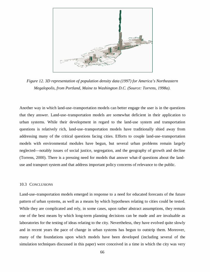
66
Figure 12. 3D representation of population density data (1997) for America’s Northeastern
Megalopolis, from Portland, Maine to Washington D.C. (Source: Torrens, 1998a).
Another way in which land-use–transportation models can better engage the user is in the questions
that they answer. Land-use–transportation models are somewhat deficient in their application to
urban systems. While their development in regard to the land-use system and transportation
questions is relatively rich, land-use–transportation models have traditionally shied away from
addressing many of the critical questions facing cities. Efforts to couple land-use–transportation
models with environmental modules have begun, but several urban problems remain largely
neglected—notably issues of social justice, segregation, and the geography of growth and decline
(Torrens, 2000). There is a pressing need for models that answer what-if questions about the land-
use and transport system and that address important policy concerns of relevance to the public.
10.3 CONCLUSIONS
Land-use–transportation models emerged in response to a need for educated forecasts of the future
pattern of urban systems, as well as a means by which hypotheses relating to cities could be tested.
While they are complicated and rely, in some cases, upon rather abstract assumptions, they remain
one of the best means by which long-term planning decisions can be made and are invaluable as
laboratories for the testing of ideas relating to the city. Nevertheless, they have evolved quite slowly
and in recent years the pace of change in urban systems has begun to outstrip them. Moreover,
many of the foundations upon which models have been developed (including several of the
simulation techniques discussed in this paper) were conceived in a time in which the city was very
67
different from its present manifestations. Those techniques are ill equipped to describe the dynamics
shaping urban evolution and are in many respects ill-suited to supporting the policy decisions that
must be made in order to manage large urban systems. Techniques such as spatial interaction
modelling focus largely on location as the driving force behind land-use and transportation patterns.
There is no doubting the significance of location in influencing these systems, but there are
additional factors that are important to consider; interaction is a crucial factor. Also, spatial
interaction models are generally static (dynamics enter these models only in an indirect fashion)
when the city is quite obviously dynamic in virtually every regard. Moreover, the spatial interaction
approach regards the city in the aggregate when it is widely accepted that local level interactions
among individuals or groups lie behind much of the behaviour that forms urban systems.
The techniques described in this paper do have many uses in urban simulation, particularly at the
levels of geography to which they are commonly applied—the zonal, aggregate, meso-and macro-
scales. However, there is an increasing awareness that urban systems are in large part dynamical
and that many of the processes responsible for forming the patterns that characterize large cities
(traffic congestion, urban sprawl, spatial structure, environmental problems, etc.) organize
themselves from the bottom up, from the repeated and myriad local-scale interaction of several
thousands of individual agents and small-scale neighbourhoods. There is a need, therefore, for the
introduction of techniques that can simulate urban systems in this fashion. Equally, the introduction
of tools that can engage a broad spectrum of users in the simulation process is long overdue, as is
the development of modules that can investigate the most pressing problems facing urban areas.
The development of hybrid models, simulations that combine the techniques discussed in this paper
with innovative ideas from complexity theory and advancements in visualization have a great deal
to offer in addressing such issues.
68
REFERENCES
Adams, D., 1994. Urban Planning and the Development Process. UCL Press, London.
Allen, P.M., 1997. Cities and Regions as Self-Organizing Systems: Models of Complexity.
Environmental Problems and Social Dynamics. Gordon and Breach Science Publishers,
Australia.
Arthur, W.B., 1990. Positive feedbacks in the economy. Scientific American, February: 80-85.
Australian Bureau of Transportation Economics, 1998. Urban Transport Models: A Review
(Working Paper 39), Department of Transport and Regional Services, Canberra, Australia.
Bahl, R.W., 1968. A land speculation model: the role of the property tax as a constraint to urban
sprawl. Journal of Regional Science, 8(2): 199-208.
Balchin, P. and Kieve, J.L., 1977. Urban Land Economics. Macmillan, London.
Barra, T.d.l., 1989. Integrated Land Use and Transport Modelling: Decision Chains and
Hierarchies. Cambridge University Press, Cambridge.
Batty, M., 1976. Urban Modelling: Algorithims, Calibrations, Predictions. Cambridge Urban and
Architectural Studies. Cambridge University Press, London.
Batty, M., 1979. Progress, success, and failure in urban modeling. Environment and Planning A, 11:
863-878.
Batty, M., 1991. Generating urban forms from diffusive growth. Environment and Planning A, 23:
511-544.
Batty, M., 1994. A chronicle of scientific planning: the Anglo-American modeling experience.
Journal of the American Planning Association, 60(1): 7-16.
Batty, M., 1997a. Cellular automata and urban form: A primer. Journal of the American Planning
Association, 63(2): 266-274.
Batty, M., 1997b. Editorial: Urban systems as cellular automata. Environment and Planning B, 24:
159-164.
Batty, M., 1998. Urban evolution on the desktop: simulation with the use of extended cellular
automata. Environment and Planning A, 30: 1943-1967.

69
Batty, M., 1999. Modeling urban dynamics through GIS-based cellular automata. Computers,
Environment and Urban Systems, 23: 205-233.
Batty, M. and Jiang, B., 1999. Multi-Agent Simulation: New Approaches to Exploring Space-Time
Dynamics Within GIS. CASA Working Paper 10, Centre for Advanced Spatial Analysis
(CASA), University College London, London.
Batty, M., Jiang, B. and Thurstain-Goodwin, M., 1998. Local Movement: Agent-Based Models of
Pedestrian Flows. CASA Working Paper 4, Centre for Advanced Spatial Analysis (CASA),
University College London, London.
Batty, M. and Longley, P., 1994. Fractal Cities. Academic Press, London.
Batty, M. and Xie, Y., 1994. From cells to cities. Environment and Planning B, 21: s31-s48.
Batty, M. and Xie, Y., 1997. Possible urban automata. Environment and Planning B, 24: 175-192.
Batty, M., Xie, Y. and Sun, Z., 1999. The dynamics of urban sprawl. CASA Working Paper 15,
University College London, Centre for Advanced Spatial Analysis (CASA), London.
Bell, M., Dean, C. and Blake, M., 1999. A model for forecasting the location of fringe urbanisation,
with GIS and 3D visualisation, Sixth International Conference on Computers in Urban
Planning and Urban Management (CUPUM), IUAV, Venice.
Benati, S., 1997. A cellular automaton for the simulation of competitive location. Environment and
Planning B, 24: 175-192.
Bonabeau, E., Dorigo, M. and Theraulaz, G., 1999. Swarm Intelligence: From Natural to Artificial
Systems. Santa Fe Institue Studies in the Sciences of Complexity. Oxford University Press,
New York.
Bramley, G., Bartlett, W. and Lambert, C., 1995. Planning, the Market and Private Housebuilding.
The Natural and Built Environment Series 4. UCL Press, London.
Cambridge Systematics, I. and Group, H.C., 1991. Making the Land Use, Transportation, Air
Quality Connection--Modelling Practices, Volume I.
Carter, H., 1981. The Study of Urban Geography. Edward Arnold, Victoria, Australia.
Cartwright, T.J., 1991. Planning and chaos theory. Journal of the American Planning Association,
57(1): 44-56.

70
Casti, J.L., 1997. Would-be Worlds: How Simulation is Changing the Frontiers of Science. John
Wiley & Sons, New York.
Centre for Advanced Spatial Analysis, 2000. Computer Visualisation for the Corporation of
London: A Review of Applications and Proposals for Implementation, Centre for Advanced
Spatial Analysis (CASA), University College London, London.
Cervero, R., 1989. America's Suburban Centers : The Land-Use Transportation Link. Unwin-
Hyman, Winchester, MA.
Clarke, K., 1997. Land transition modeling with deltatrons. Department of Geography, University
of California, Santa Barbara.
Clarke, K.C., Hoppen, S. and Gaydos, L., 1997. A self-modifying cellular automaton model of
historical urbanization in the San Francisco Bay area. Environment and Planning B, 24: 247-
261.
Couclelis, H., 1985. Cellular worlds: A framework for modeling micro-macro dynamics.
Environment and Planning A, 17: 585-596.
Couclelis, H., 1997. From cellular automata to urban models: New principles for model
development and implementation. Environment and Planning B, 24: 165-174.
Epstein, J.M. and Axtell, R., 1996. Growing Artificial Societies from the Bottom Up. Brookings
Institution, Washington D.C.
Faith, J., 1998. Why Gliders Don't Exist: Anti-Reductionism and Emergence. In: C. Adami (Editor),
Artificial Life VI: Proceedings of the Sixth International Conference on Artificial Life.
Complex Adaptive Systems, No. 6. MIT Press, Cambridge, MA.
Fotheringham, A.S., Brunsdon, C. and Charlton, M., 2000. Quantitative Geography: Perspectives
on Spatial Data Analysis. Sage, London.
Fotheringham, A.S. and O'Kelly, M.E., 1989. Spatial Interaction Models: Formulations and
Applications. Studies in Operational Regional Science. Kluwer Academic Publishers,
Dordrecht.
Golledge, R. and Stimson, R.J., 1997. Spatial Behavior: A Geographic Perspective. The Guilford
Press, New York.
71
Government of Ireland, 1995. Dublin Transportation Initiative Technical Volume I: Transport
Modelling in Phase 2. Stationary Office, Dublin.
Harris, B., 1994. The real issues concerning Lee's "Requiem". Journal of the American Planning
Association, 60(1): 31-34.
Harvey, J., 1996. Urban Land Economics. Macmillan, Houndsmills.
Hegelsmann, R. and Flache, A., 1998. Understanding complex social dynamics: a plea for cellular
automata based modelling. Journal of Artificial Societies and Social Simulation, 1(3).
Holland, J.H., 1998. Emergence: From Chaos to Order. Perseus Books, Reading, MA.
Kivell, P., 1993. Land and the City: Patterns and Processes of Urban Change. Routledge, London.
Klosterman, R.E., 1994. Large-scale urban models: retrospect and prospect. Journal of the
American Planning Association, 60(1): 3-6.
Krugman, P., 1996. The Self-Organizing Economy. Blackwell, Malden, MA.
Landis, J., 1994. The California Urban Futures Model: a new generation of metropolitan simulation
model. Environment and Planning B, 21(2).
Landis, J., 1995. Imagining land use futures: applying the California Urban Futures Model. Journal
of the American Planning Association, 61(4): 438-457.
Landis, J. and Zhang, M., 1998. The second generation of the California Urban Futures Model. Part
2: Specification and calibration results of the land-use chaneg submodel. Environment and
Planning B, 25: 795-824.
Langton, C.G., 1992. Life at the Edge of Chaos. In: C.G. Langton, C. Taylor, J.D. Farmer and S.
Rasmussen (Editors), Artificial Life II. Addison-Wesley, Redwood City, CA, pp. 41-93.
Lee, D.B., 1973. Requiem for large-scale models. Journal of the American Institute of Planners, 39:
163-178.
Lee, D.B., 1994. Retrospective on large-scale urban models. Journal of the American Planning
Association, 60(1): 35-40.
Lee, M.-S. and Goulias, K., 1997. Accessibility indicators for transportation planning using GIS,
Transportation Research Board.
Levy, S., 1992. Artificial Life: The Quest for a New Creation. Penguin Books, London.
72
Miller, E.J., Kriger, D.S. and Hunt, J.D., 1998. Integrated Urban Models for Simulation of Transit
and Land-Use Policies. TCRP Project H-12.
Nagel, K., Barrett, C.L. and Rickert, M., 1996a. Parallel traffic microsimulation by cellular
automata and application for large-scale transportation modeling. LA-UR 96-50, Los Alamos
National Laboratory, Los Alamos, NM.
Nagel, K., Beckman, R.J. and Barrett, C.L., 1999. TRANSIMS for urban planning. LA-UR 98-
4389, Los Alamos National Laboratory, Los Alamos, NM.
Nagel, K., Rasmussen, S. and Barrett, C.L., 1996b. Network traffic as self-organized critical
phenomena. TSA-DO/SA MS-M997 and CNLS MS-B258, Los Alamos National Laboratory,
Los Alamos, NM.
Nagel, K. and Schrekenberg, M., 1995. Traffic jams in stochastic cellular automata. 95ATS089, Los
Alamos National Laboratory, Los Alamos, NM.
Openshaw, S., 1979. A methodology for using models for planning purposes. Environment and
Planning A, 11: 879-896.
Openshaw, S., 1983. The Modifiable Areal Unit Problem. Catmog 38. GeoBooks, Norwich.
Oryani, K. and Harris, B., 1996. Enhancement of DVRPC's Travel Simulation Models Task 12:
Review of Land Use Models and Recommended Model for DVRPC. Report Prepared for
Delaware Valley Regional Planning Commission, URS Consultants, Inc., Philadelphia.
O'Sullivan, D., 2000a. Graph-based cellular automata models of urban spatial processes. Ph.D.
thesis Thesis, University College London, London.
O'Sullivan, D., 2000b. Using desktop GIS for the investigation of accessibility by public transport:
an isochrone approach. International Journal of Information Science, 14(1): 85-104.
Phipps, M. and Langlois, A., 1997. Spatial dynamics, cellular automata, and parallel processing
computers. Environment and Planning B, 24(193-204).
Portugali, J., Benenson, I. and Omer, I., 1997. Spatial cognitive dissonance and sociospatial
emergence in a self-organizing city. Environment and Planning B, 24: 263-285.
Putman, S.H., 1979. Urban Residential Location Models. Kluwer Academic Publishers.
Putman, S.H., 1983. Integrated Urban Models. Pion.
73
Putman, S.H., 1989. Integrated Urban Models: Policy Analysis of Transportation and Land Use.
Pion.
Putman, S.H., 1992. Integrated Urban Models 2: New Research and Applications of Optimization
and Dynamics. Pion.
Resnick, M., 1994a. Changing the centralized mind. Technology Review(July): 32-40.
Resnick, M., 1994b. Learning about life. Artificial Life, 1(1-2).
Resnick, M., 1996. Beyond the centralized mindset. Journal of the Learning Sciences, 5(1): 1-22.
Resnick, M., 1999. Turtles, Termites, and Traffic Jams: Explorations in Massively Parallel
Microworlds. Complex Adaptive Systems. MIT Press, Cambridge, MA.
Sanders, L., Pumain, D., Mathian, H., Guérin-Pace, F. and Bura, S., 1997. SIMPOP: A multiagent
system for the study of urbanism. Environment and Planning B, 24: 287-305.
Sayer, R.A., 1979. Understanding urban models versus understanding cities. Environment and
Planning A, 11: 853-862.
Schelhorn, T., O'Sullivan, D., Haklay, M. and Thurstain-Goodwin, M., 1999. STREETS: an agent-
based pedestrian model, University College London, Centre for Advanced Spatial Analysis,
London.
Schelling, T.C., 1978. Micromotives and Macrobehavior. WW Norton and Company, New York.
Sembolini, F., 1997. An urban and regional model based on cellular automata. Environment and
Planning B, 24: 589-612.
Sipper, M., 1997. Evolution of Parallel Cellular Machines: The Cellular Programming Approach.
Lecture Notes in Computer Science 1194. Springer, Berlin.
Smith, M., 1998. Painting by numbers--mathematical models of urban systems. Environment and
Planning B, 25: 483-493.
Taylor, C.E., 1992. "Fleshing Out" Artificial Life II. In: C.G. Langton, C. Taylor, J.D. Farmer and
S. Rasmussen (Editors), Artificial Life II: Proceedings of the Workshop on Artificial Life held
February, 1990 in Santa Fe, New Mexico. Addison-Wesley, Redwood City, CA, pp. 25-38.
Thomas, R.M. and Huggett, R.J., 1980. Modelling in Geography: A Mathematical Approach.
Barnes & Noble Books, Totowa, N.J.
74
Thurstain-Goodwin, M. and Unwin, D., 2000. Defining and delineating the central areas of towns
for statistical monitoring using continuous surface representations, Centre for Advanced Spatial
Analysis, University College London.
Torrens, P.M., 1998a. Everything Must Go! The Geography of Retail Change in America's
Northeastern Megalopolis, 1977 to 1992. Master's Thesis, Indiana University, Bloomington.
Torrens, P.M., 1998b. A Manhattan Made of Lego: Modeling Urban Phenomena Using Cellular
Automata, University of Washington, Seattle.
Torrens, P.M., 2000. SprawlSim: A Simulation Model for Exploring Spatial Complexity and
Sprawling Urban Growth, Centre for Adavanced Spatial Analysis (CASA), University College
London, London.
Torrens, P.M. and Alberti, M., 2000. Measuring sprawl, Centre for Advanced Spatial Analysis,
University College London and Department of Urban Design and Planning, University of
Washington.
Waddell, P., 1998a. UrbanSim Reference Guide: Beta Version, University of Washington, Seattle.
Waddell, P., 1998b. UrbanSim Specifications. Version 1.01, University of Washington, Seattle.
Wagner, D.F., 1997. Cellular automata and geographic information systems. Environment and
Planning B, 24: 219-234.
Webster, C., Wu, F. and Zhou, S., 1998. An object-based urban simulation model for interactive
visualisation, Third International Conference on GeoComputation, University of Bristol.
Wegener, M., 1983. Description of the Dortmund Region Model. Working Paper 8, Institut für
Raumplanung, Dortmund.
Wegener, M., 1994. Operational urban models: state of the art. Journal of the American Planning
Association, 60: 17-29.
Wegener, M., 1996. The potential of microsimulation for urban models. In: G.P. Clarke (Editor),
Microsimulation for Urban and Regional Policy Analysis. European Research in Regional
Science 6. Pion, London.
White, R. and Engelen, G., 1993. Cellular automata and fractal urban form. Environment and
Planning A, 25: 1175-1199.
75
White, R. and Engelen, G., 1997. Cellular automata as the basis of integrated dynamic regional
modelling. Environment and Planning B, 24: 235-246.
White, R., Engelen, G. and Uljee, I., 1997. The use of constrained cellular automata for high-
resolution modelling of urban land use dynamics. Environment and Planning B, 24: 323-343.
Wolfram, S., 1994. Cellular Automata and Complexity. Addison-Wesley, Reading, MA, 3-71 pp.
Wu, F., 1998. An experiment on the generic polycentricity of urban growth in a cellular automatic
city. Environment and Planning B, 25: 731-752.
Wu, F. and Webster, C.J., 1998. Simulation of land development through the integration of cellular
automata and multicriteria evaluation. Environment and Planning B, 25: 103-126.
Xie, Y., 1994. Analytical models and algorithims for cellular urban dynamics. Ph.D. Thesis,
University of New York at Buffalo, Buffalo, NY.