D

CCeennttrree ffoorr AAddvvaanncceedd SSttuuddiieess

RReesseeaarrcchh NNootteess

Emmanuel Farhi, Iván Werning

Capital Taxation: Quantitative Explorations

of the Inverse Euler Equation

RN #2007/03

State University - Higher School of Economics

Moscow

Centre for Advanced Studies Russia, Moscow http://www.cas.hse.ru E-mail: cas@hse.ru The Centre for Advanced Studies was created in 2006 at Higher School of Economics (HSE) in cooperation with the New Economic School. Its aim is to promote international standards of research in the socio-economic sciences in close collaboration with foreign academics to be published in English in high-level peer-reviewed journals. It involves the active participation of young Russian researchers working with their counterparts. Its approach to multidisciplinary academic studies at the frontiers of modern social sciences is organized in the framework of its Centre for Economic Policy, its International Research Program and its Program of Visiting Academics at the Higher School of Economics. The paper was presented at the International Conference "Frontiers of Macroeconomics and International Economics" organized by the Centre for Advanced Studies (HSE-NES), May 24-26, 2007, Moscow.

Capital Taxation∗

Quantitative Explorations of the

Inverse Euler Equation

Emmanuel FarhiMIT

efarhi@mit.edu

Ivan WerningMIT

iwerning@mit.edu

October 18, 2006 (3:45pm)

Abstract

This paper provides and employs a simple method for evaluating the quantitative im-

portance of distorting savings in Mirrleesian private-information settings. Our exercise

takes any baseline allocation for consumption—from US data or a calibrated equilib-

rium model using current policy—and solves for the best reform that ensures preserving

incentive compatibility. The Inverse Euler equation holds at the new optimized alloca-

tion. Our method provides a simple way to compute the welfare gains and optimized

allocation—indeed, yielding closed form solutions in some cases. When we apply it, we

find that welfare gains may be quite significant in partial equilibrium, but that gen-

eral equilibrium considerations mitigate the gains significantly. In particular, starting

with the equilibrium allocation from Aiyagari’s incomplete market model yields small

welfare gains.

∗ Werning is grateful for the hospitality of Harvard University and the Federal Reserve Bank of Minneapo-lis during the time this draft was completed. We thank comments and suggestions from Daron Acemoglu,Manuel Amador, Marios Angeletos, Patrick Kehoe, Narayana Kocherlakota, Mike Golosov, Ellen McGrat-tan, Robert Shimer, Aleh Tsyvinski and seminar participants at the Federal Reserve Bank of Minnepolis,Chicago, MIT, Harvard, Urbana-Champaign, Carnegie-Mellon, Wharton and the Conference on the Macroe-conomics of Imperfect Risk Sharing at the UC-Santa Barbara, Society for Economic Dynamics in Vancouverand the NBER Summer institute. Special thanks to Mark Aguiar, Pierre-Olivier Gourinchas, Fatih Guve-nen, Dirk Krueger, Fabrizo Perri, Luigi Pistaferri and Gianluca Violante for enlightening exchanges on theavailable empirical evidence for consumption and income. All remaining errors are our own.

1

Introduction

Recent work has upset a cornerstone result in optimal tax theory. According to Ramsey

models, capital income should eventually go untaxed (Chamley, 1986; Judd, 1985). In other

words, individuals should be allowed to save freely and without distortions at the social rate

of return to capital. This important benchmark has dominated formal thinking on this issue.

By contrast, in economies with idiosyncratic uncertainty and private information it is

generally suboptimal to allow individuals to save freely: constrained efficient allocations sat-

isfy an Inverse Euler equation, instead of the agent’s standard intertemporal Euler equation

(Diamond and Mirrlees, 1977; Rogerson, 1985; Ligon, 1998). Recently, extensions of this

result have been interpreted as counterarguments to the Chamley-Judd no-distortion bench-

mark (Golosov, Kocherlakota and Tsyvinski, 2003; Albanesi and Sleet, 2004; Kocherlakota,

2004; Werning, 2002).

This paper explores the quantitative importance of these arguments. We examine how

large welfare gains are from distorting savings and moving away from letting individuals save

freely. In the process, we also extend and develop some new theoretical ideas. The issue we

address is largely unexplored because—deriving first-order conditions aside—it is difficult to

solve dynamic economies with private information, except for some very particular cases.1

The novelty of our approach is to sidesteps these difficulties by forgoing a complete solu-

tion for both consumption and work effort, and focusing, instead, entirely on consumption.

Our exercise takes a given some baseline allocation—say, that generated in equilibrium with

the current U.S. tax code—and improves on it in a way that does not affect the work ef-

fort allocation. That is, we optimize within a set of perturbations for consumption that

guarantee preserving the incentive compatibility of the baseline work effort allocation. Our

perturbations are rich enough to yield the Inverse Euler equation as a necessary condition

for optimality, so that we fully capture recent arguments for distorting savings.

Moreover, our partial reform strategy is the relevant planning problem to address the

capital taxation issue discussed above. That is, our calculations represent the welfare gains

of moving away from allowing agents to save freely, for any given insurance arrangement, to

a situation where their savings are optimally distorted. Symmetrically, it represents the cost

of removing optimal savings distortions, for any given insurance arrangement, and allowing

individuals to save freely. It is important to emphasize that the question addressed in this

paper is not the full design of a social insurance system, but rather to evaluate the auxiliary

role that distorting savings may play in any such system. Our partial reform strategy gets

precisely at this.

1 Two special cases that have been extensively explored are unemployment and disability insurance.

2

In addition to being the relevant subproblem for the question addressed in this paper,

there are some important advantages to a partial reform approach. First, the analysis of

this problem turns out to be very tractable and flexible. As a result, one is not forced

towards overly simplified assumptions, such as the specification of uncertainty, in order to

make progress. In our view, this flexibility is important for any quantitative work.

Secondly, and most importantly, our exercise does not require fully specifying some com-

ponents of the economy. In particular, the details of the work-effort side of preferences and

technology—such as how elastic work effort is to changes in incentives, whether the problem

is one of private information regarding skills or of moral hazard regarding effort, etcetera—

are not inputs in the exercise. This is a crucial advantage since current empirical knowledge

of these things is limited and controversial. Our reforms are the richest ones one can consider

without having to take a stand on these modelling details. Thus, we are able to address the

question of how valuable it is to distort savings without evaluating the gains from selecting

correctly along the tradeoff between insurance and incentives. We think this is an important

advantage of our approach to the question we set out to answer: the welfare gains involved

in distorting savings.

This paper relates to several strands of literature. First, there is the optimal taxation lit-

erature based on models with private information (see Golosov, Tsyvinski and Werning, 2006,

and the references therein). Papers in this literature usually solve for constrained efficient

allocations subject to the assumed asymmetry of information. Second, following the seminal

paper by Aiyagari (1994), there is a vast literature on incomplete-market Bewley economies

within the context of the neoclassical growth model. These papers emphasize the role of con-

sumers self-smoothing through the precautionary accumulation of risk-free assets. In most

positive analyses, government policy is either ignored or else a simple transfer and tax sys-

tem is included and calibrated to current policies. In some normative analyses, some reforms

of the transfer system, such as the income tax or social security, are evaluated numerically

(e.g. Conesa and Krueger, 2005). Our paper bridges the gap between the optimal-tax and

incomplete-market literatures by evaluating the importance of the constrained-inefficiencies

in the latter.

The notion of efficiency used in the present paper is often termed constrained-efficiency,

because it imposes the incentive-compatibility constraints that arise from the assumed asym-

metry of information. Within exogenously incomplete-market economies, a distinct notion

of constrained-efficiency has emerged (see Geanakoplos and Polemarchakis, 1985). The idea

is roughly whether, taking the available asset structure as given, individuals could change

their trading positions in such a way that generates a Pareto improvement at the resulting

market-clearing prices. This notion has been applied by Davila, Hong, Krusell and Rios-Rull

3

(2005) to Aiyagari’s (1994) setup. They show that, in this sense, the resulting competitive

equilibrium is inefficient. In this paper we also apply our methodology to examine an effi-

ciency property of the equilibrium in Aiyagari’s (1994) model, but it should be noted that

our notion of constrained efficiency, which is based on preserving incentive-compatibility, is

very different.

We proceed as follows. Section 1 lays out the basic backbone of our model, including

assumptions regarding preferences, technology and information. Section 2 describes the per-

turbations and defines the planning problem we study. Section 3 derives a Bellman equation

representation, which serves as a methodological pillar for the rest of our analysis. Section 4

studies a partial equilibrium example that can be solved in closed form. Section 5 presents

and employs the methodology for the general equilibrium problem. Section 6 provides con-

cluding comments.

1 The Mirrleesian Economy

We cast our model within a general Mirrleesian dynamic economy. We follow the specifi-

cation in Golosov, Kocherlakota and Tsyvinski (2003) most closely. They extend previous

arguments leading to an Inverse Euler equation (e.g. Diamond and Mirrlees, 1977) by al-

lowing individuals’ privately observed skills to evolve as a general stochastic process. We

allow this generality. Indeed, we will show that our analysis also applies to extensions that

includes a very general form of moral hazard or human capital accumulation.

Preferences. A continuum of agents have the utility function

∞∑

t=0

βtE[U(ct) − V (nt; θt)] (1)

where U is the utility function from consumption and V is the disutility function from

effective units of labor (hereafter: labor for short). We assume U is increasing, concave

and continuously differentiable. Additive separability between consumption and leisure is a

feature of preferences that we adopt because it is required for the arguments leading to the

Inverse Euler equation.2

Idiosyncratic uncertainty is captured by an individual specific shock θt ∈ Θ that evolves

as a Markov process. These shocks may be interpreted as determining skills or productivity,

therefore affecting the disutility of effective units of labor. We denote the history up to

2 The intertemporal additive separability of consumption also plays a role. However, the intertem-poral additive separability of work effort is completely immaterial: we could (pedantically) replace∑

∞

t=0βt

E[V (nt; θt)] with some general disutility function V ({nt}).

4

period t by θt ≡ (θ0, θ1, . . . , θt). Uncertainty is assumed idiosyncratic, so that the {θt} is

independent and identically distributed across agents.

Allocations over consumption and labor are sequences {ct(θt)} and {nt(θ

t)}. As is stan-

dard, it is convenient to change variables, translating any consumption allocation into utility

assignments {ut(θt)}, where ut(θ

t) ≡ U(ct(θt)). This change of variable makes the incentive

constraints below linear, rendering the planning problem convex.

Information and Incentives. The shock realizations are private information to the agent,

so we must ensure that allocations are incentive compatible. We invoke the revelation prin-

ciple to derive the incentive constraints by considering a direct mechanism.

Imagine agents reporting each period their current shock realization. They are then

allocated consumption and labor as a function of the entire history of reports. The agent’s

strategy determines a report for each period as a function of the history, {σt(θt)}. The

incentive compatibility constraint requires that truth-telling, σ∗t (θ

t) = θt, be optimal:

∞∑

t=0

βtE[U(ct(θ

t)) − V (nt(θt); θt)] ≥

∞∑

t=0

βtE[U(ct(σ

t(θt))) − V (nt(σt(θt)); θt)] (2)

for all reporting strategies {σt}.

Technology. We allow for a general technology over capital and labor, that includes the

neoclassical formulation as a special case. Let Kt, Nt and Ct represent aggregate capital,

labor and consumption for period t, respectively. The resource constraints are then

G(Kt+1, Kt, Nt, Ct) ≤ 0 t = 0, 1, . . .

with initial capital K0 given. The function G(K ′, K,N,C) is assumed to be concave and

continuously differentiable, increasing in K and N and decreasing in K ′ and C.

This technology specification is very flexible. For the neoclassical growth model we simply

set G(K ′, K,N,C) = −K ′ +F (K,N) + (1− δ)K −C, where F (K,N) is a concave constant

returns production function satisfying Inada conditions FK(0, N) = ∞ and FK(∞, N) = 0.

Other technologies, such as convex adjustment costs, can just as easily be incorporated in

the specification of G.

An important simple case is linear technology: labor can be converted to output linearly,

with productivity normalized to one, and there is some storage technology with safe gross

rate of return q−1. One can think of this as partial equilibrium, perhaps representing the

situation of a small open economy facing a fixed net interest rate r = q−1−1, or as the most

stylized of A-K growth models (Rebelo, 1991). This special case fits our general setup with

G(K ′, K,N,C) = N − qK ′ +K − C. With a continuum of agents, one can summarize the

5

use of resources by their expected discounted value, using q as the discount factor.

Log Utility. Our model and its analysis, allows for general utility functions U(c). However,

the case with logarithmic utility U(c) = log(c) is of special interest for two reasons. The

first reason is that we obtain simple formulas for the welfare gains in this case. Although

the simplifications are useful, they are not in any way essential for our analysis.

More importantly, logarithmic utility is a natural benchmark for our model. Recall that,

from the outset, we adopted additive separability between consumption and labor since this

assumption is needed for the arguments leading to the Inverse Euler equation. But given

this separability a logarithmic utility function for consumption is a standard and sensible

choice. In growth models, logarithmic utility is required for balanced growth. Moreover, a

unitary coefficient of relative risk aversion and elasticity of substitution is broadly consistent

with the range of empirical evidence.

Moral Hazard. We can extend our framework to introduce moral hazard as follows. Each

period the agent takes an unobservable action et suffering some disutility, separable from

consumption. Effective labor, nt, is then a function of the history of effort and shocks, so

that nt = f(et, θt). Moreover, we can allow the distribution of θt to depend on past effort and

shocks. Such a hybrid model seems relevant for thinking about the evolution of individuals’

earned labor income—purely Mirrleesian or purely moral hazard stories are not likely to

approximate reality very well.

2 Planning Problem

The starting point for our exercise is any allocation for consumption and labor that is

incentive compatible. Given this baseline we consider a class of variations or perturbations

that preserve incentive compatibility. The perturbations we consider induce shifts in the

consumption allocation that ensure effort is unchanged. These perturbation are rich enough

to deliver the Inverse Euler equation as an optimality condition. As a result, we fully capture

the characterization of optimality stressed by Golosov et al. (2003).

2.1 Perturbations for Partial Reform

Parallel Perturbations. For any period t and history θt a feasible perturbation, of any

baseline allocation, is to decrease utility at this node by β∆ and compensate by increasing

utility by ∆ in the next period for all realizations of θt+1. Total lifetime utility is unchanged.

Moreover, since only parallel shifts in utility are involved, incentive compatibility of the new

6

allocation is preserved. We can represent the new allocation as ut(θt) = ut(θ

t) − β∆ and

ut+1(θt+1) = ut+1(θ

t+1) + ∆, for all θt+1.

This perturbation changes the allocation in periods t and t+ 1 after history θt only. The

full set of variations generalizes this idea by allowing perturbations of this kind at all nodes:

u(θt) ≡ u(θt) + ∆(θt−1) − β∆(θt)

for all sequences of {∆(θt)} such that u(θt) ∈ U(R+) and such that the limiting condition

limT→∞

βT+1E[∆(σt+T (θt+T ))] = 0

for all reporting strategies {σt}. The limiting condition rules out Ponzi-like schemes in

utility,3 so that from any strategy {σt} remaining expected utility is only changed by a

constant ∆−1:∞

∑

t=0

βtE[ut(σ

t(θt))] =

∞∑

t=0

βtE[ut(σ

t(θt))] + ∆−1. (3)

It follows directly from equation (2) that if the baseline allocation {ut} is incentive compatible

then the new allocation {ut} remains so.4 Note that the value of the initial shifter ∆−1

determines the lifetime utility of the new allocation relative to its baseline. In particular, if

∆−1 = 0 then all perturbations yield the same utility as the baseline. In particular for any

fixed infinite history θ∞

equation (3) implies that (by substituting the deterministic strategy

σt(θt) = θt)

∞∑

t=0

βtut(θt) =

∞∑

t=0

βtut(θt) + ∆−1, (4)

so that ex-post realized utility is the same along all possible realizations for the shocks.5

Let Υ({ut},∆−1) denote the set of utility allocations {ut} that can be generated by such

perturbations starting from a baseline allocation {ut} for a given initial ∆−1. This is a

convex set.

Partial Reform Problem. The problem we wish to consider takes as given a baseline

allocation {ut} and an initial ∆−1 and seeks the alternative allocation {ut} ∈ Υ({ut},∆−1)

3 Note that the limiting restrictions are trivially satisfied for all variations with finite horizon: sequencesfor {∆t} that are zero after some period T . This was the case in the discussion of a perturbation at a singlenode and its successors.

4 It is worth noting that in the logarithmic utility benchmark case parallel additive shifts in utilityrepresent proportional shifts in consumption.

5 The converse is nearly true: by taking appropriate expectations of equation (4) one can deduceequation (3), but for a technical caveat involving the possibility of inverting the order of the expectationsoperator and the infinite sum (which is always possible in a version with finite horizon and Θ finite). Thiscaveat is the only difference between equation (3) and equation (4).

7

that maximizes expected utility subject to the technological constraints. We want to allow

for the possibility that in the initial period individuals are heterogeneous with respect to

their shock, θ0. We capture this without burdening the notation by letting the expectations

operator integrate over the initial distribution for θ0 in the population, in addition to future

shocks.

Planning Problem

max{ut},Ct,Kt+1,∆−1

∞∑

t=0

βtE[ut(θ

t)]

subject to,

{ut} ∈ Υ({ut},∆−1)

G(Kt+1, Kt, Nt, Ct) ≥ 0 Ct = E[c(ut(θt))] t = 0, 1, . . . (5)

where the cost function c ≡ u−1 represents the inverse of the utility function U(c).

This problem maximizes expected discounted utility within the set of feasible perturba-

tions subject to an aggregate resource constraint (5). Note that from equation (3) we know

that the objective function equals ∆−1 plus the utility from the baseline allocation.

2.2 Inverse Euler equation

In this section we review briefly the Inverse Euler equation which is the optimality condition

for our planning problem.

Proposition 1. At an interior optimum for the partial reform problem

βc′(ut) = qtEt[c′(ut+1)] ⇒

1

u′(ct)=qtβ

Et

[

1

u′(ct+1)

]

. (6)

where qt ≡ R−1t and

Rt ≡ −GC,t

GK ′,t

GK,t+1

GC,t+1

is the technological rate of return, i.e. the technologically feasible tradeoff dCt+1/dCt.

Equation (6) is the so called Inverse Euler equation. The important point is that our

perturbations are rich enough to recover the crucial optimality condition stressed in Golosov

et al. (2003).

It is useful to contrast equation (6) with the standard Euler equation that obtains in

incomplete market models. In models where agents can save freely at the rate of return to

8

capital we obtain

u′(ct) = β Rt Et[u′(ct+1)]. (7)

Note that equation (6) is a reciprocal of sorts version of equation (7). Applying Jensen’s

inequality to equation (6) implies that at the optimum

u′(ct) < β Rt Et[u′(ct+1)]. (8)

To use Rogerson’s (1985) language: at the optimum equation (8) implies that individuals are

‘savings constrained’. Alternatively, another interpretation is that at the optimum a version

of equation (7) can hold if we substitute the social rate of return Rt for a lower private rate

of return—this difference in such rates of return is has been termed ‘distortion’, ‘wedge’ or

‘implicit tax’.

Regardless of the interpretation, the optimum cannot allow agents to save freely at tech-

nology’s rate of return, since then equation (7) would hold as a necessary condition, which

we know is incompatible with the planner’s optimality condition, equation (6). This is in

stark contrasts with the Chamley-Judd benchmark obtained in Ramsey models, where it is

optimal to let agents save freely at the technological rate of return to capital.

We now consider a subproblem that takes as given aggregate consumption and savings,

and only optimizes over the distribution of this aggregate consumption. Of course, this is

the only relevant problem for version of the economy without capital; but it is also of interest

because of its relation to some welfare decompositions we shall perform later. We recover a

variant of equation (6) equivalent to that obtained by Ligon (1998).

Proposition 2. Consider the subproblem that replaces the resource constraints in (5) with

the constraint that E[c(ut(θt))] ≤ Ct for t = 0, 1, . . ., where {Ct} is any given sequence for

aggregate consumption. Then at an interior optimum there must exist a sequence of discount

factors {qt} such that for all histories θt:

Et

[

u′(ct)

u′(ct+1)

]

=β

qtt = 0, 1, . . . (9)

Equation (9) simply states that the expected ratio of marginal utilities is equalized across

agents and histories, but not necessarily linked to any technological rate of transformation.

Conditions equalizing marginal rates of substitution are standard in exchange economies.

However, unlike the standard condition obtained in an incomplete market equilibrium model,

here it is the expectation of u′(ct)/u′(ct+1), instead of u′(ct+1)/u

′(ct), that is equated. Note

9

that the implication in equation (6) is stronger, since it implies equation (9) but also pins

down qt.

2.3 Steady States with CRRA

We now focus on steady states for the planning problem, where aggregates are constant over

time. For purposes of comparison, we discuss the conditions in the context of the neoclassical

growth model specification of technology. We also limit our discussion to constant relative

risk aversion (CRRA) utility functions U(c) = c1−σ/(1 − σ). Finally, we suppose that the

baseline allocation features constant aggregate labor Nt = N .

At a steady state level of capital Kss the discount factor is constant qt = qss ≡ 1/(1+rss)

where

rss = FK(Kss, N) − δ.

With CRRA preferences the Inverse Euler equation is

Et[cσt+1] = (1 + rss)βc

σt (10)

At a steady state we must have constant consumption Ct = Css. With logarithmic utility

σ = 1 the equation above implies, by the law of iterated expectations, that

Ct+1 ≡ E[ct+1] = (1 + rss)βE[ct] ≡ (1 + rss)β Ct.

Hence, consumption is constant if and only if (1+ rss)β = 1. For σ > 1, we can use Jensen’s

inequality to obtain Et[ct+1] ≤ (β/q)1/σ ct, so it follows that Ct+1 ≤ (β/q)1/σCt. Then, if

(1+rss)β < 1 aggregate consumption Ct would strictly fall over time, contradicting a steady

state with constant positive consumption. The argument for σ < 1 is symmetric.

Proposition 3. Suppose CRRA preferences U(c) = c1−σ/(1 − σ) with σ > 0. Then at a

steady state of the planning problem

(i) if σ ≥ 1 then rss ≥ β−1 − 1

(ii) if σ ≤ 1 then rss ≤ β−1 − 1

We depict steady state equilibria by adapting a graphical device introduced by Aiyagari

(1994). For any given interest rate r we solve a fictitious planning problem with a linear

savings technology with q ≡ (1+r)−1; equivalently, this is the partial equilibrium. Intuitively,

for qss = (1 + rss)−1 the steady state for the fictitious planning coincides with the for the

actual general equilibrium planning problem—Section 5.3 formalizes this notion.

10

A(r)

F (K)-

A

C

D

B

K

r

-1-1

> 1

< 1

= 1

Figure 1: Steady States: Market Equilibrium vs. Planner. The intersection point A rep-resents the baseline market equilibrium. Points B, C and D represent, respectively, theplanner’s steady states for log utility, σ > 1 and σ < 1.

To find the equilibrium we imagine solving these fictitious planning problems for all

arbitrary r. Let C(r) denote the average steady state consumption as a function of r;

one can show that this function is increasing, which is intuitive since a higher r makes

providing future (long run) consumption cheaper to the planner. Define K(r) to be the

solution to the steady state resource constraint C(r) = F (K, N) − δk, for k ≤ kg, where

kg ≡ arg maxK{F (K, N) − δK} is the golden rule level of capital.6

In Figure 1 the unique steady state capital and interest rate (Kss, rss) is then found at

the intersection of the downward sloping schedule r = FK(K, N)−δ with the upward sloping

K(r) schedule. For comparison, the figure also displays the equilibrium schedule for steady-

state average savings, A(r), that is obtained from the incomplete markets model in Aiyagari

(1994). The steady state equilibrium level of capital is always higher than the steady state

optimum; the interest rate r is always lower.

3 A Useful Bellman Equation

We now study the case with a constant rate of discount q. The resource constraints can

then be reduced to a single expected present value condition. One literal interpretation

6If r is so high that C(r) > F (kg , N)− δkg then C(r) cannot be sustainable as a steady state. Hence, welimit ourselves to values of r for which C(r) ≤ F (kg, N) − δkg.

11

is that this represents an economy with a linear saving technology. It also represents a

‘partial-equilibrium’ component of the ‘general-equilibrium’ planning problem. In any case,

the analysis we develop here will be useful later in Section 5, when we return to the problem

with general technology.

With a fixed discount factor q the (dual of the) planning problem minimizes the expected

discounted cost∞

∑

t=0

qtE[c(ut)] =

∞∑

t=0

qtE[c(ut + ∆t − β∆t+1)]

Let K(∆−1; θ0) denote the lowest achievable expected discounted cost over all feasible per-

turbation {ut} ∈ Υ({ut},∆−1). Since both the objective and the constraints are convex it

follows immediately that the value function K(∆−1; θ0) is convex in ∆−1.

Recursive Baseline Allocations. We wish to approach the planning problem recursively.

This leads us to be interested in situations where the effects shocks θt on the baseline allo-

cation can be summarized by some state st that evolves as a Markov process. In any period

the assignment of utility is determined by this state and write the allocation as u(st).

The requirement that the baseline allocation be expressible in terms of some state variable

st is hardly restrictive. It is satisfied by virtually all baseline allocations of interest. To

see this, recall that the exogenous shock θt is a Markov process. Most economic models

then imply that consumption is a function of the full state st = (xt, θt), where xt is some

endogenous state with law of motion xt = G(xt−1, θt). The endogenous state and its law

of motion depends on the particular economic model generating the baseline allocation. A

leading example in this paper is the case of incomplete market models, such as the Bewley

economies in Huggett (1993) and Aiyagari (1994). In these models, described in more detail

in Section 5.2, individuals are subject to exogenous shocks to income or productivity and

can save using a riskless asset. The endogenous state for any individual is their asset wealth

and the law of motion is their optimal saving rule.7

A Bellman equation. We now reformulate the above planning problem recursively for

such recursive baseline allocations. First, since the problem can be indexed by s0 instead

of θ0 we rewrite the value function as K(∆−1, s0). The value function K must satisfy the

following Bellman equation.

7 Another example are allocations generated by some dynamic contract. The full state variable thenincludes the promised continuation utility (see Spear and Srivastava, 1987) along with the exogenous state.

12

Bellman equation

K(∆; s) = min∆′

[

c(u(s) + ∆ − β∆′) + qE[K(∆′; s′) | s]]

(11)

Moreover, the new optimized allocation from the sequential partial reform problem must be

generated by the policy function from the Bellman equation.

Note that from the planner’s point of view the state st evolves exogenously. Thus, the

recursive formulation takes st as an exogenous shock process and employs ∆ as an endogenous

state variable. In words, the planner keeps track of the additional lifetime utility ∆t−1 it has

previously promised the agent up and above the welfare entitled by the baseline allocation.

Note that the resulting dynamic program is very simple: the endogenous state variable ∆ is

one-dimensional and the optimization is convex.

Inverse Euler equation (again). The first-order and envelope conditions are

βc′(u(s) + ∆ − β∆′) = qE[K∆(∆′; s′) | s],

K∆(∆; s) = c′(u(s) + ∆ − β∆′).

Combining these two conditions leads to the Inverse Euler equation equation (6).

A Useful Analogy. The planning problem admits an analogy with a consumer’s income

fluctuation problem that is both convenient and enlightening. We transform variables by

changing signs and switch the minimization to a maximization. Let ∆ ≡ −∆, K(∆; s) ≡

−K(−∆; s) and U(x) ≡ −c(−x). Note that the pseudo utility function U is increasing,

concave and satisfies Inada conditions at the extremes of its domain.8 Reexpressing the

Bellman equation (11) using these transformation yields:

K(∆; s) = max∆′

[

U(−u(s) + ∆ − β∆′) + qE[K(∆′; s′) | s]]

.

This reformulation can be read as the problem of a consumer with a constant discount factor

q facing a constant gross interest rate 1+ r = β−1, entering the period with pseudo financial

wealth ∆, receives a pseudo labor income shock −u(s). The fictitious consumer must decide

how much to save β∆′; pseudo consumption is then x = −u(s) + ∆ − β∆′.

8 An important case is when the original utility function is CRRA U(c) = c1−σ/(1 − σ) for σ > 0 andc ≥ 0. Then for σ > 1 the function U(x) is proportional to a CRRA with coefficient of relative risk aversionσ = σ/(σ − 1) and x ∈ (0,∞). For σ < 1 the pseudo utility U is “quadratic-like”, in that it is proportionalto −(−x)ρ for some ρ > 1, and x ∈ (−∞, 0].

13

The benefit of this analogy is that the income fluctuations problem has been extensively

studied and used; it is at the heart of most general equilibrium incomplete market models

(Aiyagari, 1994). Intuition and results have accumulated with long experience.

Log Magic. With logarithmic utility, a case we argued earlier constitutes an important

benchmark, the Bellman equation can be simplified considerably. The idea is best seen

through the analogy, noting that the pseudo utility function is exponential −e−x in this

case. It is well known that for a consumer with CARA preferences a one unit increase in

financial wealth, ∆, results in an increase in pseudo-consumption, x, of r/(1 + r) = 1− β in

parallel across all periods and states of nature. It is not hard to see that this implies that

the value function takes the form K(∆; s) = e−(1−β)∆k(s).

Of course, this decomposition translates directly to the original value function. Less

obvious is that it greatly simplifies the Bellman equation and its solution.

Proposition 4. With logarithmic utility the value function is given by

K(∆; s) = e(1−β)∆k(s),

where function k(s) solves the Bellman equation

k(s) = Ac(s)1−β (E[k(s′) | s])β, (12)

where A ≡ (q/β)β/(1 − β)1−β.

The optimal policy for ∆ can be obtained from k(s) using

∆′ = ∆ −1

βlog

(

(1 − β)k(s)

c(s)

)

. (13)

Proof. See Appendix A.

This solution is nearly closed form: we need only compute k(s) using the recursion in

equation (12), which requires no optimization. It is noteworthy that no simplifications on

the stochastic process for skills are required.

4 Example: Random Walk in Partial Equilibrium

Although the main virtue of our approach is that we can flexibly apply it to various baseline

allocations (and we will!) in this section we begin with a simple and instructive case. We

take the baseline allocation to be a geometric random walk and center our discussion around

logarithmic utility. The advantage is that we obtain closed-form solutions for the optimized

14

allocation, the intertemporal wedge and the welfare gains. The transparency of the exercise

reveals important determinants for the magnitude of welfare gains.

Although extremely stylized, a random walk is an important conceptual and empirical

benchmark. First, most theories—starting with the simplest permanent income hypothesis—

predict that consumption should be close to a random walk. Second, some authors have ar-

gued that the empirical evidence on income, which is a major determinant for consumption,

and consumption itself shows the importance of a highly persistent component (e.g. Storeslet-

ten, Telmer and Yaron, 2004). For these reasons, a parsimonious statistical specification for

consumption may favor a random walk.

An Example Economy. Indeed, one can construct an example economy where a geometric

random walk for consumption arises as a competitive equilibrium with incomplete markets.

To see this, suppose that individuals have CRRA utility over consumption—logarithmic

utility being a special case—and disutility V (n; θ) = v(n/θ) for some convex function v(n)

over work effort n, so that θ can be interpreted as productivity. Skills evolve as a geometric

random walk, so that θt+1 = εt+1θt, where εt+1 is i.i.d. Individuals can only accumulate a

riskless asset paying return R equal to the rate of return on the economy’s linear savings

technology. They face the sequence of budget constraints

at+1 + ct ≤ Rat + θtnt t = 0, 1, . . .

and the borrowing constraint that at ≥ 0. Suppose the rate of return R is such that

1 ≥ βRE[ε−1]. Finally, suppose that individuals have no initial assets, so that a0 = 0.

In the competitive equilibrium of this example individuals exert a constant work effort

n, satisfying nv′(n) = 1, and consume all their labor income each period, ct = θtn; no assets

are accumulated, at remains at zero. This follows because the construction ensured that

the agent’s intertemporal Euler equation holds at the proposed equilibrium consumption

process. The level of work effort n is defined so that the intra-period consumption-leisure

optimality condition holds. Then, since the agent’s problem is convex, it follows that this

allocation is optimal for individuals. Since the resource constraint trivially holds, it is an

equilibrium.

Although this is certainly a very special example economy, it illustrate that a geometric

random walk for consumption is a possible equilibrium outcome.

Value Function. We now simply assume that at the baseline s′ = ε · s with ε i.i.d. and

c = s, so that u(s) = U(s). The next result follows almost immediately from Proposition 4.

Proposition 5. If consumption is a geometric random and the utility function is logarithmic,

15

then the value function and policy functions are

K(∆; s) = c(s)1

1 − βexp((1 − β)∆) g

β

1−β , (14)

∆′ = ∆ −1

1 − βlog(g), (15)

where g ≡ (q/β)E[ε].

Proof. With logarithmic utility the value function is of the form K(∆, s) = exp((1 −

β)∆)k(s) where k(s) given by Proposition 4. With a geometric random walk the problem

is homogeneous and it follows that k(s) = κs, for some constant κ. Solving for κ using

equation (12), gives equation (14). Then Equation (13) delivers equation (15).

In this example, the Inverse Euler equation is simply g ≡ (q/β)E[ε] = 1. Hence, g − 1

measures the departure of the baseline allocation from it. We next show that g−1 is critical

in determining the magnitude of the intertemporal corrective wedge and the welfare gains

from the optimized allocation.

Allocation. Using equation (15) we can express the new optimized consumption as

c(s,∆) = exp(U(s) + ∆ − β∆′) = gβ

1−β s exp((1 − β)∆).

Since equation (15) also implies that

exp((1 − β)∆′) = g−1 exp((1 − β)∆),

it follows that the new consumption allocation is also a geometric random walk. Indeed, it

equals the baseline up to a multiplicative deterministic factor that grows exponentially:

ct =β

q

εt

E[εt]ct−1 = αg−tct. (16)

The drift in the new consumption allocation is β/q, ensuring that the Inverse Euler equation

ct = (q/β)Et[ct+1] holds at the optimized allocation.

Intertemporal Wedge. Suppose the agent’s Euler equation holds at the baseline allocation:

1 =β

qE

[

ctct+1

]

=β

qE

[

ε−1]

. (17)

We can then solve for the intertemporal wedge τ at the new allocation that makes the agent’s

16

euler equation hold:

1 =β

q(1 − τ)E

[

ctct+1

]

=β

q(1 − τ)gE

[

ε−1]

. (18)

By using equation (16) in combination with equations (17) and (18) yield

τ = 1 −1

g. (19)

Applying Jensen’s inequality to equation (17) gives

1

g=β

q

1

E[ε]<β

qE

[

ε−1]

= 1 ⇒ τ > 0.

This example the Inverse Euler equation provides a rationale for a constant and positive

wedge in the agent’s Euler equation. This is in stark contrast to the Chamley-Judd bench-

mark result, where no such distortion is optimal in the long run, so that agents are allowed

to save freely at the social rate of return.

Welfare Gains. Evaluating the value function, given by equation (14), at ∆ = 0 gives the

expected discounted cost of the new optimized allocation. The baseline allocation, on the

other hand, costs sψ with

sψ = s+ qE[sεψ] ⇒ ψ =1

1 − qE[ε].

The relative reduction in costs is then

sψ

sk(0)=

ψ

k(0)=

1 − β

1 − qE[ε]g−

β

1−β =β−1 − 1

β−1 − gg−

β

1−β . (20)

By homogeneity, the ratio of costs does not depend on the level of the current shock s. Note

that at g = 1 there are no cost reductions. This is because, as discussed above, in this case

the Inverse Euler holds at the baseline allocation. At the other extreme, as g → β−1 the

cost reductions become arbitrarily large. The reason is that then qE[ε] → 1, implying that

the present value of the baseline consumption allocation goes to infinity; in contrast, k(0)

remains finite.

The variance of consumption growth. Given the importance of g, we now investigate

its main determinants. We can back out g if assume the agent’s Euler equation holds at the

17

baseline allocation and that ε is lognormally distributed. The latter assumption implies that

E[

ε−1]

= exp

(

−µ+σ2

ε

2

)

and E[

ε]

= exp

(

µ+σ2

ε

2

)

.

⇒ E[

ε]

· E[

ε−1]

= exp(σ2ε).

Multiplying and dividing the agent’s Euler equation, (β/q)E[ε−1] = 1, by E[ε] and rearrang-

ing:

g = E[

ε]

· E[

ε−1]

= exp(σ2ε)

⇒ g ≈ 1 + σ2ε.

Hence, we find that the crucial parameter g is associated with the variance in the growth

rate of consumption. Equation (19) gives τ = 1 − exp(−σ2ε), or approximately

τ ≈ σ2ε. (21)

Thus, the intertemporal wedge τ is approximately equal to the variance in the growth rate

of consumption σ2ε.

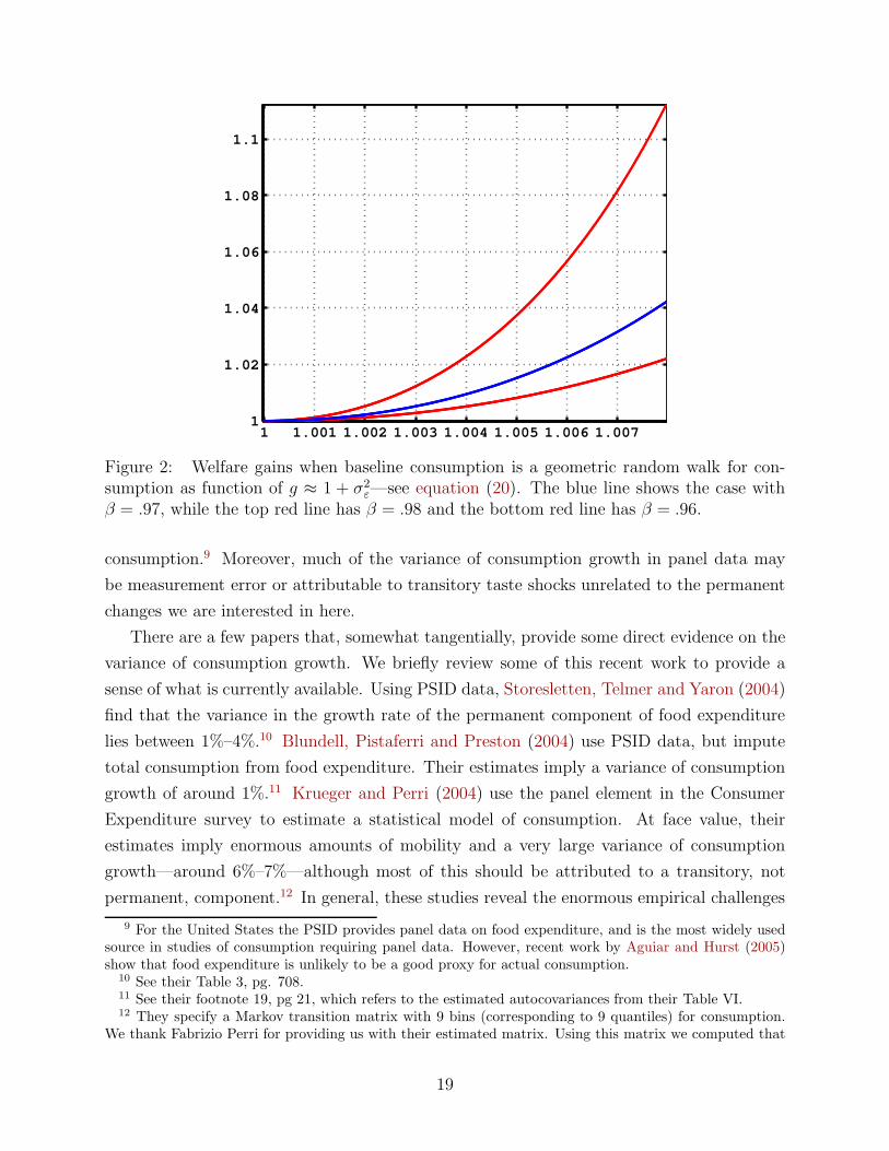
Quantitative Stab. Figure 2 plots the reciprocal of the relative cost reduction using

equation (20), a measure of relative welfare gains. The blue line is for β = .97, while the

top and bottom red lines are for β = .98 and β = .96, respectively. The figure uses an

empirically relevant range for g ≈ 1 + σ2ε.

In the figure the effect of the discount factor β is nearly equivalent to increasing the

variance of shocks; that is, moving from β = .96 to β = .98 has the same effect as doubling σ2ε.

To understand this, interpret the lower discounting not as a change in the actual subjective

discount, but as calibrating the model to a shorter period length. But then holding the

variance of the innovation between periods constant implies an increase in uncertainty over

any fixed length of time. Clearly, what matters is the amount of uncertainty per unit of

discounted time.

Empirical Evidence. Suppose one wishes to accept the random walk specification of con-

sumption as a useful empirical approximation. What does the available empirical evidence

say about the crucial parameter σ2ε?

Unfortunately, the direct empirical evidence on the variance of consumption growth is

very scarce, due to the unavailability of good quality panel data for broad categories of

18

1 1.001 1.002 1.003 1.004 1.005 1.006 1.0071

1.02

1.04

1.06

1.08

1.1

Figure 2: Welfare gains when baseline consumption is a geometric random walk for con-sumption as function of g ≈ 1 + σ2

ε—see equation (20). The blue line shows the case withβ = .97, while the top red line has β = .98 and the bottom red line has β = .96.

consumption.9 Moreover, much of the variance of consumption growth in panel data may

be measurement error or attributable to transitory taste shocks unrelated to the permanent

changes we are interested in here.

There are a few papers that, somewhat tangentially, provide some direct evidence on the

variance of consumption growth. We briefly review some of this recent work to provide a

sense of what is currently available. Using PSID data, Storesletten, Telmer and Yaron (2004)

find that the variance in the growth rate of the permanent component of food expenditure

lies between 1%–4%.10 Blundell, Pistaferri and Preston (2004) use PSID data, but impute

total consumption from food expenditure. Their estimates imply a variance of consumption

growth of around 1%.11 Krueger and Perri (2004) use the panel element in the Consumer

Expenditure survey to estimate a statistical model of consumption. At face value, their

estimates imply enormous amounts of mobility and a very large variance of consumption

growth—around 6%–7%—although most of this should be attributed to a transitory, not

permanent, component.12 In general, these studies reveal the enormous empirical challenges

9 For the United States the PSID provides panel data on food expenditure, and is the most widely usedsource in studies of consumption requiring panel data. However, recent work by Aguiar and Hurst (2005)show that food expenditure is unlikely to be a good proxy for actual consumption.

10 See their Table 3, pg. 708.11 See their footnote 19, pg 21, which refers to the estimated autocovariances from their Table VI.12 They specify a Markov transition matrix with 9 bins (corresponding to 9 quantiles) for consumption.

We thank Fabrizio Perri for providing us with their estimated matrix. Using this matrix we computed that

19

faced in understanding the statistical properties of household consumption dynamics from

available panel data.

An interesting indirect source of information is the cohort study by Deaton and Paxson

(1994). This paper finds that the cross-sectional inequality of consumption rises as the cohort

ages. The rate of increase then provides indirect evidence for σ2ε; their point estimate implies

a value of σ2ε = 0.0069. However, recent work using a similar methodology finds much lower

estimates (Slesnick and Ulker, 2004; Heathcote, Storesletten and Violante, 2004).

We conclude that, in our view, the available empirical evidence does not provide reliable

estimates for the variance of the permanent component of consumption growth. Thus, for

our purposes, attempts to specify the baseline consumption process directly are impractical.

That is, even if one were willing to assume the most stylized and parsimonious statistical

specifications for consumption, the problem is that the key parameter remains largely un-

known. This suggests that a preferable strategy is to use consumption processes obtained

from models that have been successful at matching the available data on consumption and

income.

Lessons. Two lessons emerge from our simple exercise. First, welfare gains are potentially

far from trivial. Second, they are quite sensitive to two parameters available in our exercise:

the variance in the growth rate of consumption and the subjective discount factor.

Based on the empirical uncertainty regarding these parameters, the second point suggests

obtaining the baseline allocation from a model, instead of attempting to do so directly from

the data. In addition, another reason for starting from a model is to address an important

caveat in the previous exercise, the assumed linear accumulation technology. As we shall see,

with a more standard neoclassical technology welfare gains are generally greatly tempered.

5 General Equilibrium

Up to now the analysis has been that of partial equilibrium. Alternatively one can interpret

the results as applying to an economy facing some given constant rate of return to capital.

We now argue that this magnifies the welfare gains from reforming the consumption allo-

cation. Specifically, with a concave accumulation technology, as in the neoclassical growth

model, the welfare effects may be greatly reduced. This point is certainly not surprising,

nor is it specific to the model or forces emphasized here. Indeed, a similar issue arises in

the Ramsey literature, the quantitative effects of taxing capital greatly depend on the un-

the conditional variance of consumption growth had an average across bins of 0.0646 (this is for the year2000, the last in their sample; but the results are similar for other years).

20

derlying technology.13 Unsurprising as it may, it is important to confront this issue to reach

meaningful quantitative conclusions.14

To make the point clear, consider for a moment the opposite extreme: the economy has no

savings technology, so that Ct ≤ Nt for t = 0, 1, . . . (Huggett, 1993). In this case, if the utility

function is of the CRRA form then a baseline geometric random walk allocation is constrained

efficient. This follows using Proposition 2 since one can verify that equation (9) holds. Thus,

in this exchange economy there are no welfare gains from changing the allocation.

Certainly the fixed endowment case is an extreme example, but it serves to illustrate

that general equilibrium considerations are extremely important. For a neoclassical growth

model the welfare gains lie somewhere between the endowment economy and the economy

with a fixed rate of return; where exactly, is precisely what we explore next.

5.1 Log Utility: Separation of Aggregate and Idiosyncratic

Aggregate and Idiosyncratic Subproblems. We now derive a strong separation result

that greatly simplifies the general equilibrium problem for the logarithmic utility function

case. To simplify the presentation, we shall assume that the baseline allocation features

constant aggregate labor supply Nt; this is implied whenever the baseline allocation is at

a steady state. To simplify the notation, we drop N and write the resource constraints as

G(Kt+1, Kt, Ct) ≥ 0 for t = 0, 1 . . .

First, without loss in generality, one can always decompose any allocation into an id-

iosyncratic and an aggregate component: ut(θt) = ut(θ

t) + δt; the aggregate component

{δt} is a deterministic sequence; the idiosyncratic component {ut} has constant expected

consumption normalized to one: E[c(ut(θt))] = 1. Since our feasible perturbations certainly

allow parallel deterministic shifts it follows that

{ut} ∈ Υ({ut},∆−1) ⇐⇒ {ut} ∈ Υ(

{ut},∆−1 +∞

∑

t=0

βtδt

)

.

Since ∆−1 is a free variable in the General Equilibrium Problem, this implies that we only

need to ensure that {ut} is a feasible perturbation for some value of the free variable ∆−1 =

13 Indeed, Stokey and Rebelo (1995) discuss the effects of capital taxation in representative agent en-dogenous growth models. They show that the effects on growth depend critically on a number of modelspecifications. They then argue in favor of specifications with very small growth effects, suggesting that aneoclassical growth model with exogenous growth may provide an accurate approximation.

14 A similar point is at the heart of Aiyagari’s (1994) paper, which quantified the effects on aggregatesavings of uncertainty with incomplete markets. He showed that for given interest rates the effects couldbe enormous, but that the effects were relatively moderate in the resulting equilibrium of the neoclassicalgrowth model.

21

∆−1 +∑∞

t=0 βtδt.

All the arguments up to this point apply for any utility function. However, with loga-

rithmic utility δt = log(Ct) and it follows that the planning problem can be decomposed as

follows.

General Equilibrium Problem with Log utility

max{ut},Ct,Kt+1,∆−1

[

∑

t

βtE[ut(θ

t)] +∑

t

βtU(Ct)

]

subject to,

G(Kt+1, Kt, Ct) ≥ 0 t = 0, 1, . . . (22)

E[c(ut(θt))] = 1 t = 0, 1, . . . (23)

{ut} ∈Υ({ut}, ∆−1)

It is now apparent that we can study the idiosyncratic component problem of choosing

{ut}, from the aggregate one of of selecting {Ct, Kt+1}. The aggregate variables {Ct, Kt+1}

maximize the objective function subject only to the resource constraint (22).

Aggregate Component Problem

maxCt,Kt+1

∑

t

βtU(Ct)

subject to

G(Kt+1, Kt, Ct) ≥ 0 t = 0, 1, . . .

In other words, the problem is simply that of a standard deterministic growth model, which,

needless to say, is straightforward to solve.

The idiosyncratic component problem finds the best perturbation with constant con-

sumption over time.

22

Idiosyncratic Component Problem

max{ut},∆−1

∑

t

βtE[ut(θ

t)]

subject to

E[c(ut(θt))] = 1 t = 0, 1, . . .

{ut} ∈Υ({ut}, ∆−1)

Moreover, the idiosyncratic problem can be solved by solving a partial equilibrium prob-

lem with with q = β. This follows since the Inverse Euler equation then implies that

Et[ct+1] = ct, so that aggregate consumption is constant. Hence, we can find the solution

using Proposition 4.

5.2 Quantifying the Welfare Gains

In this section we explore welfare gains quantitatively taking general equilibrium effects

into full account, using the methodology developed above for logarithmic utility. We first

replicate Aiyagari’s (1994) seminal incomplete markets exercise. We then take the general

equilibrium allocation from this model as our baseline.

Aiyagari considered a Bewley economy—where a continuum of agents each solve an

income fluctuations problem—imbedded within the neoclassical growth model. The time

horizon is infinite. There is no aggregate uncertainty, yet individuals are confronted with

significant idiosyncratic risk: after-tax labor income is stochastic. Efficiency labor is specified

directly as a first-order autoregressive process in logarithms:

log(nt) = ρ log(nt−1) + (1 − ρ) log(n) + εt

where εt is an i.i.d. random variable assumed Normally distributed. With a continuum of

agents the average efficiency labor supplied is n. Labor income is given by the product w nt

where w is the steady-state wage.

There are no market insurance arrangements, so agents must cope with their risk. They

can do so by accumulating assets, and possibly borrowing, at a constant interest rate r. The

budget constraints are

at+1 + ct ≤ (1 + r)at + wnt

23

for all t = 0, 1, . . . and histories of shocks. In addition the agent is subject to some borrowing

limit at ≥ a; we take Aiyagari benchmark, where there is no borrowing a = 0.

The equilibrium steady-state wage is given by the marginal product of labor w =

Fn(Kss, n) and the interest rate is given by the net marginal product of capital, r =

FK(Kss, n) − δ.15 For any given interest rate, individual saving behavior leads to an invari-

ant cross-sectional distribution of asset holdings. At a steady-state equilibrium the interest

rate induces a distribution with average assets equal to the capital stock K. The individual

consumption allocation is a function of assets and current income, so that it can be written

as a function of the state variable st ≡ (at, yt) which evolves as a Markov process.

Table 1 shows the computed equilibrium interest rates and the implied welfare properties

with logarithmic utility; the rest of the parameters are quite standard: the discount factor

β = .96 the production function is Cobb-Douglas with a share of capital set to 0.36, capital

depreciation is set to 0.08. This is done for various combinations of the autocorrelation

coefficient and the standard deviation of income growth (comparable to Aiyagari’s Table II,

pg. 678). We also break down the total welfare gains into the the idiosyncratic and aggregate

components.

Aiyagari argues, based on various sources of empirical evidence, for a parameterization

with a coefficient of autocorrelation of ρ = 0.6 and a standard deviation of labor income

growth of 20%. For this preferred specification, we find that welfare gains are minuscule.

This contrasts sharply with the partial equilibrium exercises and illustrates the importance

of general equilibrium effects. Relatively small welfare gains are also obtained for higher

values of ρ or the variance of income growth. Welfare gains become non-negligible, up to

around 1%, only when income shocks display extreme persistence and variance.

Overall, welfare gains appear to be very modest—especially when compared to the par-

tial equilibrium exercise in the previous section. To understand these findings it is useful

to discuss the idiosyncratic and aggregate components separately. Our finding that idiosyn-

cratic gains are modest could have perhaps been anticipated by our illustrative geometric

random-walk example, where idiosyncratic gains are zero. Intuitively, welfare gains from the

idiosyncratic component require differences in the expected consumption growth rate across

individuals. When individuals smooth their consumption over time effectively the remaining

differences are small—as a result, so are the welfare gains.

Welfare gains from the aggregate component are directly related to the difference between

the equilibrium and optimal stead-state capital. With logarithmic utility this is equivalent,

15 For simplicity this assumes no taxation. It is straightforward to introduce taxation. However, weconjecture that since taxation of labor income acts as insurance, it effectively reduces the variance of shocksto net income. Lower uncertainty will then only lower the welfare gains we compute.

24

to the difference between the equilibrium steady-state interest rate and β−1 − 1, the interest

rate that obtains with complete markets. Hence, our finding of low aggregate welfare gains

is directly related to Aiyagari’s (1994) main conclusion: precautionary savings are small in

the aggregate, in that steady-state capital and interest rate are close their complete-markets

levels, as shown in our Table 1. Our exercise establishes that general equilibrium effects

crucial, not just for such positive quantitative conclusions, but also for normative ones.

Std(log(nt) − log(nt−1)) = .2Welfare Gains

ρ r Idiosyncratic Aggregate Total0 4.1467% .006% ∼ 0% 0.006%0.3 4.1260% 0.018% ∼ 0% 0.018%0.6 4.0856% 0.05% 0.001% 0.051%0.9 3.9493% 0.19% 0.008% 0.198%

Std(log(nt) − log(nt−1)) = .4Welfare Gains

ρ r Idiosyncratic Aggregate Total0 4.0149% 0.06% 0.004% 0.064%0.3 3.9067% 0.15% 0.012% 0.162%0.6 3.7113% 0.40% 0.039% 0.439%0.9 3.3036% 1.16% 0.15% 1.31%

Table 1: Welfare Gains for replication of Aiyagari (1994).

To get a feel for the magnitudes, Figure 3 computes aggregate welfare gains as a function

of the initial condition, expressed in terms of the difference between the baseline steady-

state rate of interest Rss = F ′(k0) + 1 − δ and β−1. The gains are non-linear and convex

shaped. The figure illustrates why the gains from the aggregate component are quite modest

in Table 1: the largest difference in interest rates is less than 1% in the table, but it takes a

much larger difference, of around 2%, to get welfare gains that are bigger than 1%.

5.3 General Utility

Relaxed Problem. A fruitful way of attacking the problem for general preferences is to

consider a relaxed version that replaces the sequence of constraints Ct = E[c(ut(θt))] for

t = 0, 1, . . . with a single present value condition. This relaxed problem takes as given a

sequence of intertemporal prices {Qt} used to compute the present value.

25

−0.03 −0.02 −0.01 0 0.01 0.02 0.03 0.04 0.05 0.06 0.070

0.005

0.01

0.015

0.02

0.025

0.03

0.035

0.04

0.045

0.05

change in interest rate

wel

fare

gai

n

Figure 3: Aggregate component of welfare gains for logarithmic utility as a function of theinitial interest rate difference: (F ′(k0) + 1 − δ) − β−1.

Relaxed Problem

max{ut},Ct,Kt+1,∆−1

∑

t

βtE[ut(θ

t)]

subject to,

G(Kt+1, Kt, Ct) ≥ 0 t = 0, 1, . . .∞

∑

t=0

QtCt =

∞∑

t=0

QtE[c(ut(θt))] (24)

{ut} ∈ Υ({ut},∆−1)

The connection with the original problem is the following. If the prices {Qt} induce a

solution to the relaxed problem that has Ct = E[c(ut(θt))] holding for all t = 0, 1, . . . then

this also solves the original problem. Indeed, one can interpret {Qt} as Lagrange multipliers;

appealing to a Lagrangian necessity theorem then ensures the existence of such a sequence

{Qt}. This ‘relaxed problem’ approach is adopted from Farhi and Werning (2005).

The vantage point of this approach is that it decouples the aggregate and idiosyncratic

parts of the problem. As a result, as long as the baseline allocation can be written recursively

as a function of some state variable s, one can solve for the consumption allocation using

a Bellman equation similar to the one from Section 2. To see this, note that the relaxed

26

problem must solve the dual that minimizes expected discounted costs, given by (24), subject

to delivering a certain promised lifetime utility level. If one parameterizes the promised

utility level, relative to the baseline, by ∆−1 and let qt ≡ Qt+1/Qt we obtain the following

representation.

Nonstationary Bellman equation

K(∆; s, t) = min∆′

[

c(u(s) + ∆ − β∆′) + qtE[K(∆′; s′, t+ 1) | s]]

Indeed, an economy that converges to a steady-state has qt converging to some constant

value q, so a stationary Bellman as in Section 2 then characterizes the long run. In this

sense, the analysis of the dynamic programming problem with given q remains relevant.

As for the aggregate sequence of capital it is trivially determined by the first order

condition from the relaxed problem. This directly pins down the sequence {Kt} given the

sequence of prices {Qt}. Reversely, any sequence of capital {Kt} can be associated one-to-one

with a sequence of relative prices {Qt+1/Qt}.

In principle, the entire problem, including the transitional dynamics, can then be solved

numerically by a shooting algorithm taking aim at the identified steady state, which can be

found using the method behind Figure 1. One can compute simple upper and lower bounds

on the welfare gains that include the transition, without the need to fully solve for it.

Simple Upper and Lower Welfare Bounds

Simple upper and lower bounds can be computed for the welfare gains that are likely to be

very informative. We suppose the baseline allocation initially finds itself at a steady state.

Upper Bound. We start with the upper bound. The idea is simple, we replace the actual

concave production function F (k) + (1 − δ)k with a linear one tangent at the new steady

state: F (k) ≡ F ′(Kss)(K−Kss)+F (Kss)+(1− δ)Kss. We then solve the planning problem

given this technology. This problem is simple because it is equivalent to a stationary relaxed

problem with q = F ′(kss)−1. The welfare improvement then constitutes an upper bound to

the true gains since the technology F is better than F .

Lower Bound. Moving on to the lower bound, the idea is simply to not solve the full

maximization. Instead, one can take any allocation for utility {ut} ∈ Υ({ut},∆−1), and

for any such sequence consider the best feasible allocation generated from parallel shifts

ut(θt) = ut(θ

t) + υt for a deterministic sequence {υt}. Define the sequence of consumption

functions Ψt(υt) = E[c(ut(θt) + υt)]. Then the problem reduces to the deterministic general

27

equilibrium problem

max{Ct}

∞∑

t=0

βtΨ−1t (Ct)

G(Kt+1, Kt, Ct) ≥ 0 t = 0, 1, . . .

and welfare is the value of this problem and the discounted expected value from the allocation

{ut}. The allocation {ut} used in this exercise can be any feasible perturbation, but there

are sensible and simple choices. For example, one can simply use the baseline allocation, or

alternatively, the solution from the relaxed problem for some arbitrary sequence of prices

{qt}. A simple case would be to use a constant value of q, say, that from the new steady

state qss. One can indeed use many allocations to produce many such lower bounds and use

the highest value thus obtained.

6 Conclusions

This main contribution of this paper is to provide a method for evaluating the auxiliary role

that distortions on savings may play in social insurance arrangements. In particular, it can

be used evaluate the welfare importance of recent ‘Inverse Euler’ arguments for distorting

savings and capital accumulation based.

Several insights emerge from our current explorations employing this method. In partic-

ular, we found that welfare gains may be arbitrarily large in partial-equilibrium settings, but

that general-equilibrium effects tend to greatly temper these gains. In fact, for the Aiyagari

(1994) incomplete-market benchmark we found relatively modest gains. We isolates two

features that contribute towards welfare gains: (i) the degree of mean reversion in consump-

tion; and (ii) the amount of aggregate precautionary savings. Both are not too significant

in Aiyagari’s benchmark economy, explaining our findings of small welfare gains.

We believe that the methodological contribution of this paper transcends our own quan-

titative explorations of it. The method developed here is flexible enough to accommodate

several extensions and it may be of interest to investigate how these may affect the quantita-

tive conclusions found here for the benchmark Aiyagari economy. In a separate paper (Farhi

and Werning, 2006) we pursue two such extensions. The first is to consider overlapping-

generations demographics instead of the dynastic setup used here. Another, is to Epstein-Zin

preferences that separate risk aversion from the intertemporal elasticity of substitution.

28

Appendix

A Proof of Proposition 4

With logarithmic utility the Bellman equation is

K(s,∆) = min∆′

[s exp(∆ − β∆′) + qE[K(s′,∆′) | s]]

= min∆′

[s exp((1 − β)∆ + β(∆ − ∆′)) + qE[K(s′,∆′) | s]]

Substituting that K(∆, s) = k(s) exp((1 − β)∆) gives

k(s) exp((1 − β)∆) = min∆′

[s exp((1 − β)∆ + β(∆ − ∆′)) + qE[k(s′) exp((1 − β)∆′) | s]],

and cancelling terms:

k(s) = min∆′

[s exp(β(∆ − ∆′)) + qE[k(s′) exp((1 − β)(∆′ − ∆)) | s]]

= mind

[s exp(−βd) + qE[k(s′) exp((1 − β)d) | s]]

= mind

[s exp(−βd) + qE[k(s′) | s] exp((1 − β)d)]

where d ≡ ∆′ − ∆. We can simplify this one dimensional Bellman equation further. Define

q(s) ≡ qE[k(s′) | s]/s and

M(q) ≡ min[exp(−βd) + q exp((1 − β)d)].

The first-order conditions gives

β exp(−βd) = q(1 − β) exp((1 − β)d) ⇒ d = logβ

(1 − β)q. (25)

Substituting back into the objective we find that

M(q) =1

1 − βexp(−βd) =

1

1 − βexp

(

−β logβ

(1 − β)q

)

=1

(1 − β)1−βββqβ = Bqβ,

where B is a constant defined in the obvious way in terms of β.

29

The operator associated with the Bellman equation is then

T [k](s) = sM

(

qE[k(s′) | s]

s

)

= As1−β (E[k(s′) | s])β,

where A ≡ Bqβ = (q/β)β/(1 − β)1−β.

Combining the Bellman k(s)/s = M(q) = Aqβ with equation (25) yields the policy

function as a function of K(s). This completes the proof.

30

References

Aguiar, Mark and Erik Hurst, “Consumption versus Expenditure,” Journal of PoliticalEconomy, 2005, 113 (5), 919–948. 19

Aiyagari, S. Rao, “Uninsured Idiosyncratic Risk and Aggregate Saving,” Quarterly Journalof Economics, 1994, 109 (3), 659–684. 1, 3, 4, 10, 11, 12, 14, 21, 23, 24, 25, 28

Albanesi, Stefania and Christoper Sleet, “Dynamic Optimal Taxation with PrivateInformation,” 2004. mimeo. 2

Blundell, Richard, Luigi Pistaferri, and Ian Preston, “Consumption inequality andpartial insurance,” IFS Working Papers W04/28, Institute for Fiscal Studies 2004. 19

Chamley, Christophe, “Optimal Taxation of Capital in General Equilibrium,” Economet-rica, 1986, 54, 607–22. 2

Conesa, Juan Carlos and Dirk Krueger, “On the Optimal Progressivity of the IncomeTax Code,” Journal of Monetary Economics, 2005, forthcoming. 3

Davila, Julio, Jay H. Hong, Per Krusell, and Jose-Victor Rios-Rull, “Con-strained efficiency in the neoclassical growth model with uninsurable idiosyncraticshocks,” PIER Working Paper Archive 05-023, Penn Institute for Economic Re-search, Department of Economics, University of Pennsylvania July 2005. available athttp://ideas.repec.org/p/pen/papers/05-023.html. 3

Deaton, Angus and Christina Paxson, “Intertemporal Choice and Inequality,” Journalof Political Economy, 1994, 102 (3), 437–67. 20

Diamond, Peter A. and James A. Mirrlees, “A Model of Social Insurance With VariableRetirement,” Working papers 210, Massachusetts Institute of Technology, Department ofEconomics 1977. 2, 4

Farhi, Emmanuel and Ivan Werning, “Inequality, Social Discounting and ProgressiveEstate Taxation,” NBER Working Papers 11408 2005. 26

and , “Quantifying the Gains from Savings Distortions: The Role of Risk Aversionand Finite Lives,” 2006. work in progress. 28

Geanakoplos, John and Heracles M. Polemarchakis, “Existence, Regularity, and Con-strained Suboptimality of Competitive Allocations When the Asset Market Is Incomplete,”Cowles Foundation Discussion Papers 764, Cowles Foundation, Yale University 1985. avail-able at http://ideas.repec.org/p/cwl/cwldpp/764.html. 3

Golosov, Mikhail, Aleh Tsyvinski, and Ivan Werning, “New Dynamic Public Finance:A User’s Guide,” forthcoming in NBER Macroeconomics Annual 2006, 2006. 3

, Narayana Kocherlakota, and Aleh Tsyvinski, “Optimal Indirect and Capital Tax-ation,” Review of Economic Studies, 2003, 70 (3), 569–587. 2, 4, 6, 8

31

Heathcote, Jonathan, Kjetil Storesletten, and Giovanni L. Violante, “Two Viewsof Inequality Over the Life-Cycle,” Journal of the European Economic Association (Papersand Proceedings), 2004, 3, 543–52. 20

Huggett, Mark, “The risk-free rate in heterogeneous-agent incomplete-insuranceeconomies,” Journal of Economic Dynamics and Control, 1993, 17 (5–6), 953–969. 12,21

Judd, Kenneth L., “Redistributive Taxation in a Perfect Foresight Model,” Journal ofPublic Economics, 1985, 28, 59–83. 2

Kocherlakota, Narayana, “Zero Expected Wealth Taxes: A Mirrlees Approach to Dy-namic Optimal Taxation,” 2004. mimeo. 2

Krueger, Dirk and Fabrizio Perri, “On the Welfare Consequences of the Increase in In-equality in the United States,” in Mark Gertler and Kenneth Rogoff, eds., NBER Macroe-conomics Annual 2003, Cambridge, MA: MIT Press, 2004, pp. 83–121. 19

Ligon, Ethan, “Risk Sharing and Information in Village Economics,” Review of EconomicStudies, 1998, 65 (4), 847–64. 2, 9

Rebelo, Sergio, “Long-Run Policy Analysis and Long-Run Growth,” Journal of PoliticalEconomy, 1991, 99 (3), 500–521. 5

Rogerson, William P., “Repeated Moral Hazard,” Econometrica, 1985, 53 (1), 69–76. 2,9

Slesnick and Ulker, “Inequality and the Life-Cycle: Consumption,” Technical Report2004. 20

Spear, Stephen E. and Sanjay Srivastava, “On Repeated Moral Hazard with Discount-ing,” Review of Economic Studies, 1987, 54 (4), 599–617. 12

Stokey, Nancy L. and Sergio Rebelo, “Growth Effects of Flat-Rate Taxes,” Journal ofPolitical Economy, 1995, 103 (3), 519–50. 21

Storesletten, Kjetil, Chris I. Telmer, and Amir Yaron, “Cyclical Dynamics in Id-iosyncratic Labor Market Risk,” Journal of Political Economy, 2004, 112 (3), 695–717.15, 19

Werning, Ivan, “Optimal Dynamic Taxation,” 2002. PhD Dissertation, University ofChicago. 2

32