centre for wireless communications wireless ad hoc & sensor networks nordic radio symposium 2004...
Post on 20-Dec-2015
213 views
TRANSCRIPT

Centre for Wireless Communications
Wireless Ad Hoc & Sensor Networks
Nordic Radio Symposium 2004August 16 – 18, 2004University of Oulu, Finland
Presenter: Carlos Pomalaza-Ráez
http://www.ee.oulu.fi/~carlos/NRS_04_Tutorial.ppt
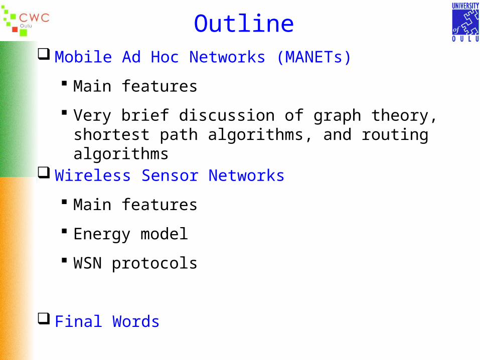
OutlineMobile Ad Hoc Networks (MANETs)
Main features
Very brief discussion of graph theory, shortest path algorithms, and routing algorithms
Wireless Sensor Networks
Main features
Energy model
WSN protocols
Final Words
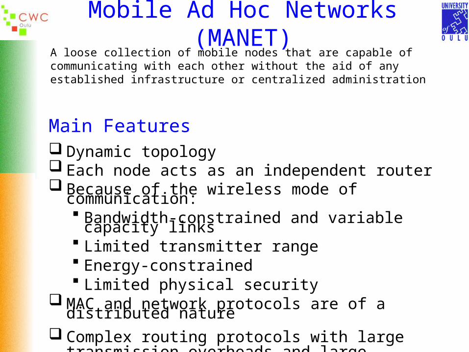
Mobile Ad Hoc Networks (MANET)
A loose collection of mobile nodes that are capable of communicating with each other without the aid of any established infrastructure or centralized administration
Main Features Dynamic topology Each node acts as an independent router Because of the wireless mode of communication:
Bandwidth-constrained and variable capacity links Limited transmitter range Energy-constrained Limited physical security
MAC and network protocols are of a distributed nature Complex routing protocols with large transmission
overheads and large processing loads on each node
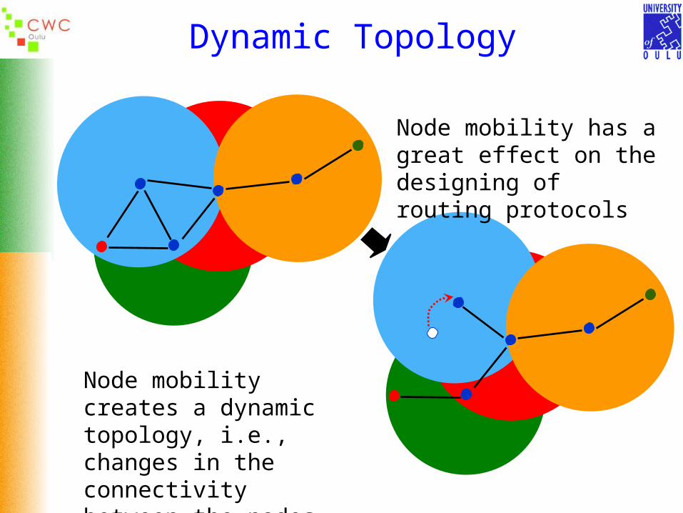
Dynamic Topology
Node mobility has a great effect on the designing of routing protocols
Node mobility creates a dynamic topology, i.e., changes in the connectivity between the nodes
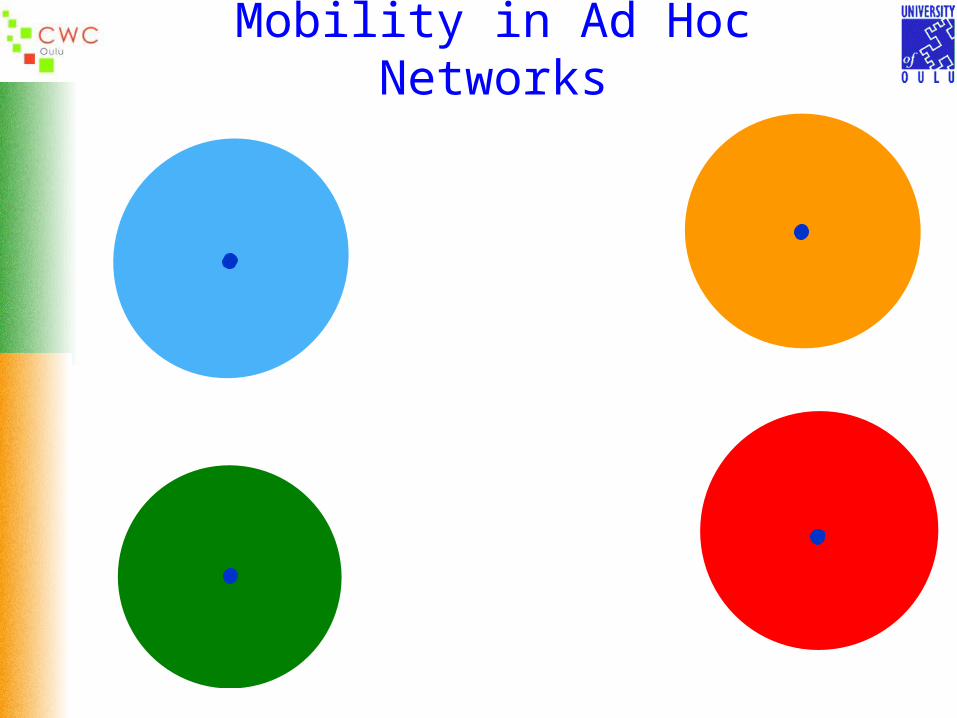
Mobility in Ad Hoc Networks
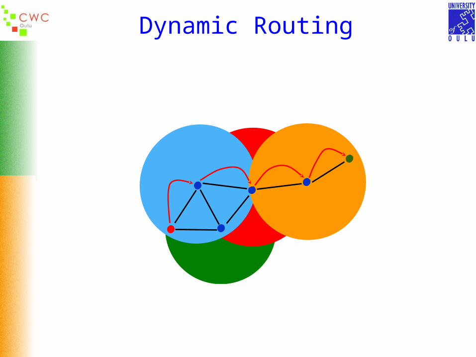
Dynamic Routing

Route Maintenance
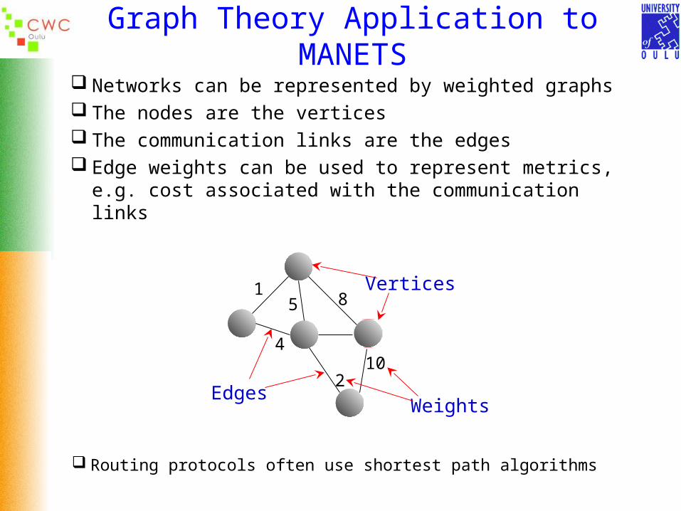
Graph Theory Application to MANETS
Networks can be represented by weighted graphs The nodes are the vertices The communication links are the edges Edge weights can be used to represent metrics, e.g. cost
associated with the communication links
Routing protocols often use shortest path algorithms
Vertices
Edges
1
102
85
4
Weights
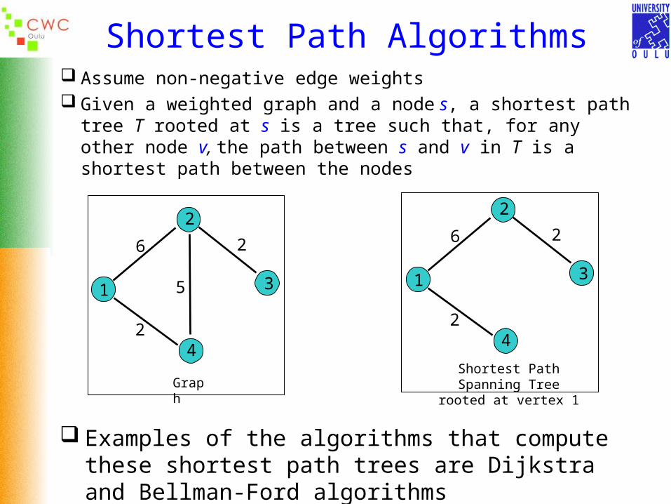
Shortest Path Algorithms Assume non-negative edge weights Given a weighted graph and a node s, a shortest path tree T
rooted at s is a tree such that, for any other node v, the path between s and v in T is a shortest path between the nodes
Examples of the algorithms that compute these shortest path trees are Dijkstra and Bellman-Ford algorithms
2
4
31
6 2
5
2
Graph
2
4
31
6 2
2
Shortest Path Spanning Treerooted at vertex 1

Distributed Asynchronous Shortest Path Algorithms
Each node computes the path with the shortest weight to every network node
There is no centralized computation Control messaging is required to distribute the
computation Asynchronous means here that there is no
requirement of inter-node synchronization for the computation performed at each node for the exchange of messages between nodes

Routing Protocols
Desired Properties Distributed Consider both uni- and bi-directional links Energy efficient Secure
Performance Metrics Data throughput Delay Overhead costs Power consumption
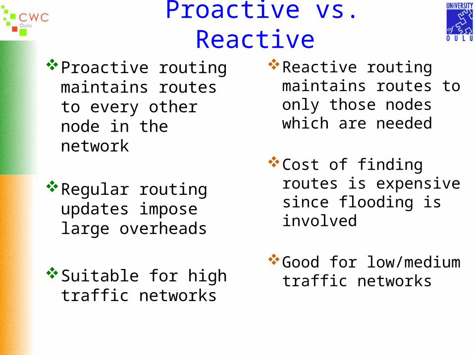
Proactive vs. Reactive
Proactive routing maintains routes to every other node in the network
Regular routing updates impose large overheads
Suitable for high traffic networks
Reactive routing maintains routes to only those nodes which are needed
Cost of finding routes is expensive since flooding is involved
Good for low/medium traffic networks

AODV – Path Finding
A B
G
D
E
H
node discards packets that have been seen
S
D
C
F
source broadcastsa route request packet
neighbors re-broadcast the packet until it reaches the intended destination
reply packet follows the reverse path of the route request packet recorded in broadcast packet
RREQ
RREP
node discards packets that have been seen

Traditional Routing Protocols
SourceDestination
Problems Energy depletion in certain nodes Not suitable for Wireless Sensor Networks
Consider several routes
Find the best
Then use it as much as possible
Wireless Sensor Networks
What is a sensor?A device that produces a measurable response to a change in a physical or chemical condition, e.g. temperature, ground composition
Sensor Networks A large grouping of low-cost, low-power, multifunctional, and small-sized sensor nodes
They benefit from advances in 3 technologies:
• digital circuitry• wireless communication• silicon micro-machining
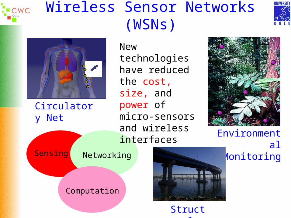
Wireless Sensor Networks (WSNs)
Sensing
Computation
Networking
Circulatory Net
EnvironmentalMonitoring
Structural
New technologies have reduced the cost, size, and power of micro-sensors and wireless interfaces
Some Applications of WSNs
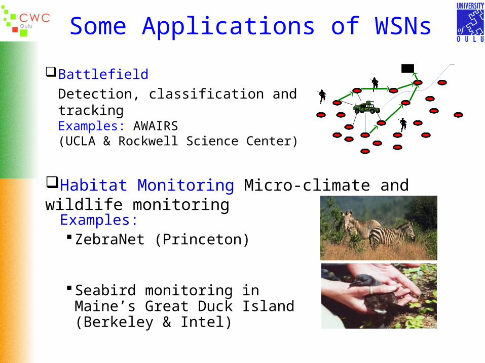
Battlefield
Detection, classification and trackingExamples: AWAIRS (UCLA & Rockwell Science Center)
Examples:ZebraNet (Princeton)
Seabird monitoring in Maine’s Great Duck Island (Berkeley & Intel)
Habitat Monitoring Micro-climate and wildlife monitoring
Some Applications of WSNs
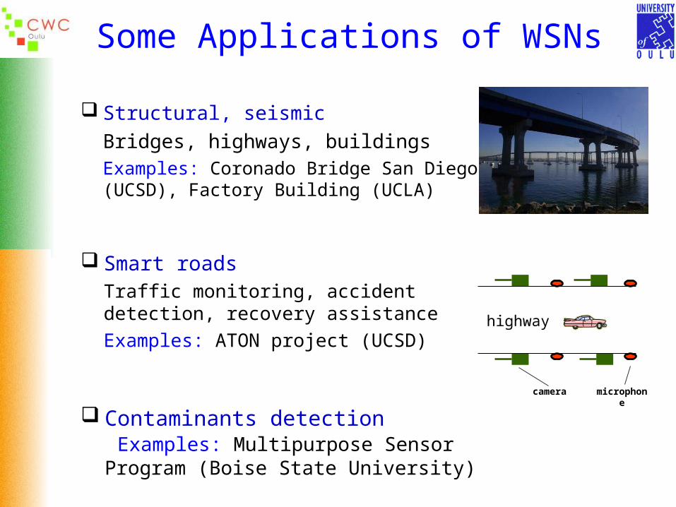
Structural, seismic
Bridges, highways, buildingsExamples: Coronado Bridge San Diego (UCSD), Factory Building (UCLA)
Smart roadsTraffic monitoring, accident detection, recovery assistance
Examples: ATON project (UCSD)highway
camera microphone
Contaminants detection Examples: Multipurpose Sensor Program (Boise State University)
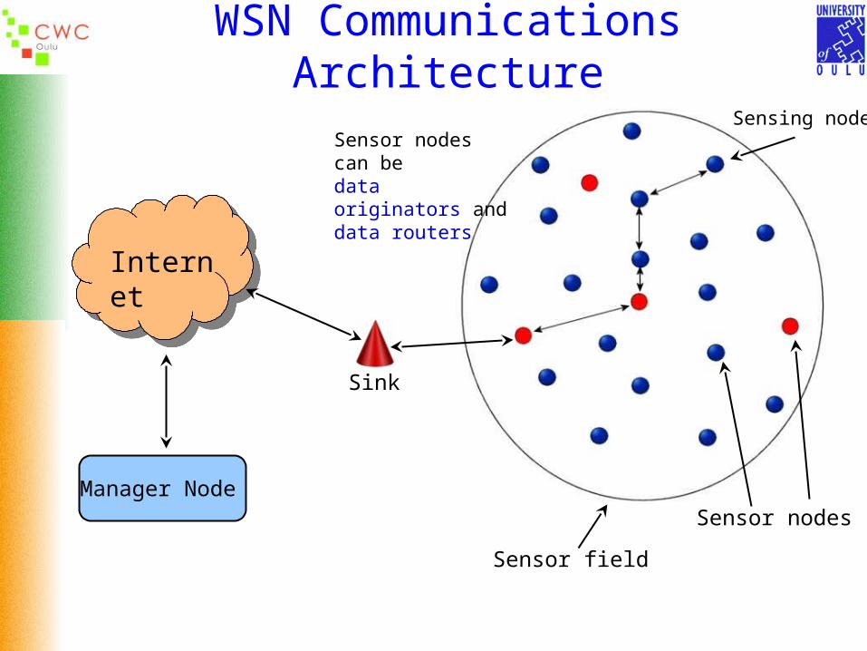
WSN Communications Architecture
Sensor field
Sensor nodes
Internet
Sink
Manager Node
Sensing nodeSensor nodes can bedata originators anddata routers
Examples of Sensor Nodes

Sensor Node Evolution
Mote Type WeC ReneRene
2Dot Mica
Date Sep-99 Oct-00 Jun-01 Aug-01 Feb-02
Microcontroller (4MHz)
Type AT90LS8535 ATMega163ATMega103/12
8
Prog. mem. (KB) 8 16 128
RAM (KB) 0.5 1 4
Communication
Radio RFM TR1000
Rate (Kbps) 10 10/40
Modulation Type OOK OOK/ASK

Typical Features of WSNs
A very large number of nodes Asymmetric flow of information Communications are triggered by queries or events At each node there is a limited amount of energy Almost static topology Low cost, size, and weight per node Prone to failures Broadcast communications instead of point-to-point Nodes do not have a global ID such as an IP number Limited security
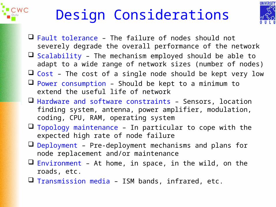
Design Considerations
Fault tolerance – The failure of nodes should not severely degrade the overall performance of the network
Scalability – The mechanism employed should be able to adapt to a wide range of network sizes (number of nodes)
Cost – The cost of a single node should be kept very low Power consumption – Should be kept to a minimum to extend the useful
life of network Hardware and software constraints – Sensors, location finding system,
antenna, power amplifier, modulation, coding, CPU, RAM, operating system
Topology maintenance – In particular to cope with the expected high rate of node failure
Deployment – Pre-deployment mechanisms and plans for node replacement and/or maintenance
Environment – At home, in space, in the wild, on the roads, etc. Transmission media – ISM bands, infrared, etc.
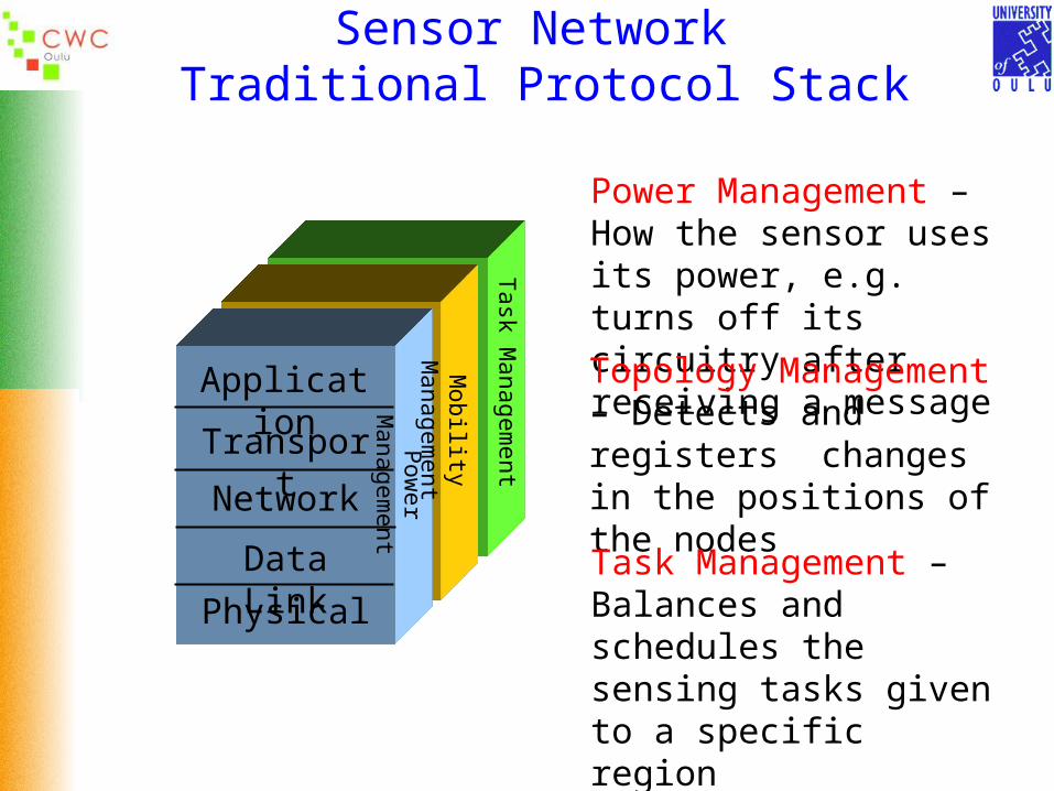
Sensor Network Traditional Protocol Stack
Transport
Data Link
Physical
Network
Pow
er
Managem
ent
Application
Mobility
Managem
ent
Task M
anagem
ent
Power Management – How the sensor uses its power, e.g. turns off its circuitry after receiving a message
Topology Management – Detects and registers changes in the positions of the nodes
Task Management – Balances and schedules the sensing tasks given to a specific region

Physical Layer
Physical
Data Link
Network
Transport
Application Frequency selection
ISM bands have often been proposed Carrier frequency generation and signal detection
Aim for simplicity, low power consumption, and low cost per unit
ModulationBinary modulation schemes are simpler to implement and thus deemed to be more energy-efficient for WSN applications
Low transmission power and simple transceiver circuitry make Ultra Wideband (UWB) an attractive candidate
Physical Layer
Energy consumption minimization is of paramount importance when designing the physical layer for WSN in addition to the usual factors such as scattering, shadowing, reflection, diffraction, multipath, and fading
Energy Limitations
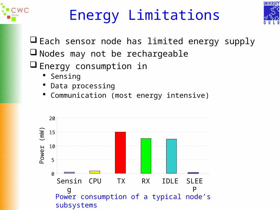
Power consumption of a typical node’s subsystems
0
5
10
15
20
Pow
er
(mW
)
Sensing
CPU TX RX
IDLE SLEEP
Each sensor node has limited energy supply Nodes may not be rechargeable Energy consumption in
Sensing Data processing Communication (most energy intensive)

CWC WIRO (WIreless Research Object )
RF Board
Tx Rx SleepCPLD 3mA/3.3V 9.9mW 3mA/3.3V 9.9mW 0.01mA/3.3V 0.033mW
RF-Transceiver
10mA/3.3V 33mW 5.8mA/3.3V 19mW 0.7μA/3.3V 0.0023mW
Other Circuitry
0.5mA/5V 2.5mW 0.5mA/5V 2.5mW 0.5mA/5V 2.5mW
RF Board TotalPower Consumption
45.5
31.5
2.5
0
10
20
30
40
50
Pow
er (
mW
)
Tx Rx Sleep
CPU Board 2 Euro coin & RF Board WIRO Box

Node Energy Model
A typical node has a sensor system, A/D conversion circuitry, DSP and a radio transceiver. The sensor system is very application dependent. The communication components consume most of the energy.
A simple model for a wireless link is:

Energy Model
The energy consumed when sending a packet of m bits over a one hop wireless link can be expressed as:
decodestRRencodestTTL ETPmEETPdmEdmE )(),(),(
where,ET = energy used by the transmitter circuitry and power
amplifierER = energy used by the receiver circuitryPT = power consumption of the transmitter circuitryPR = power consumption of the receiver circuitryTst = startup time of the transceiverEencode = energy used to encodeEdecode = energy used to decode
Transmitter Receiver

Energy Model
Assuming a linear relationship for the energy spent per bit at the transmitter
and receiver circuitry ET and ER can be written as,
deemdmE TATCT ),(
RCR memE )(
where eTC, eTA, and eRC are hardware dependent parameters and α is the path loss exponent whose value varies from 2 (for free space) to 4 (for multipath channel models).
The effect of the transceiver startup time, Tst, will greatly depend on the type of MAC protocol used. To minimize power consumption it is desirable to have the transceiver in a sleep mode as much as possible. However, constantly turning the transceiver on and off to bring it to readiness for transmission or reception also consumes energy.
Energy Model
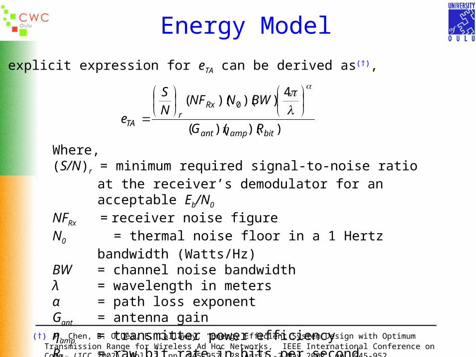
An explicit expression for eTA can be derived as(†),
))()((
4))()(( 0
bitampant
Rxr
TA RG
BWNNFN
S
e
Where,(S/N)r = minimum required signal-to-noise ratio at the receiver’s
demodulator for an acceptable Eb/N0
NFRx = receiver noise figureN0 = thermal noise floor in a 1 Hertz bandwidth (Watts/Hz)BW = channel noise bandwidthλ = wavelength in metersα = path loss exponent Gant = antenna gainηamp = transmitter power efficiencyRbit = raw bit rate in bits per second
(†) P. Chen, B. O’Dea, E. Callaway, “Energy Efficient System Design with Optimum Transmission Range for Wireless Ad Hoc Networks,” IEEE International Conference on Comm. (ICC 2002), Vol. 2, pp. 945-952, 28 April -2 May 2002, pp. 945-952.

Energy Model
The expression for eTA can be used for those cases where a particular hardware configuration is being considered. The dependence of eTA on (S/N)r can be made more explicit if the previous equation is written as:
))()((
4))()((
ere wh0
bitampant
Rx
rTA RG
BWNNF
NSe
This expression shows explicitly the relationship between eTA and (S/N)r.
The probability of bit error p depends on Eb/N0 which in turns depends
on (S/N)r.
Eb/N0 is independent of the data rate. In order to relate Eb/N0 to (S/N)r,
the data rate and the system bandwidth must be taken into account, i.e.,

Energy Model
TbTbr BRBRNENS 0
where
Eb = energy required per bit of informationR = system data rate
BT = system bandwidth
γb = signal-to-noise ratio per bit, i.e., (Eb/N0)
Modulation MethodTypical Bandwidth
(Null-To-Null)
QPSK, DQPSK 1.0 x Bit Rate
MSK 1.5 x Bit Rate
BPSK, DBPSK, OFSK 2.0 x Bit Rate
Typical Bandwidths for Various Digital Modulation Methods
Energy Model
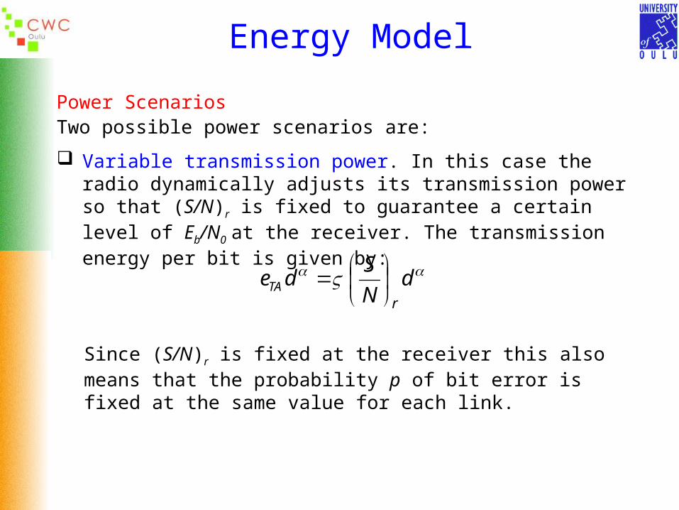
Power ScenariosTwo possible power scenarios are:
Variable transmission power. In this case the radio dynamically adjusts its transmission power so that (S/N)r is fixed to guarantee a certain level of Eb/N0 at the receiver. The transmission energy per bit is given by:
dN
Sde
rTA
Since (S/N)r is fixed at the receiver this also means that the probability p of bit error is fixed at the same value for each link.
Energy Model
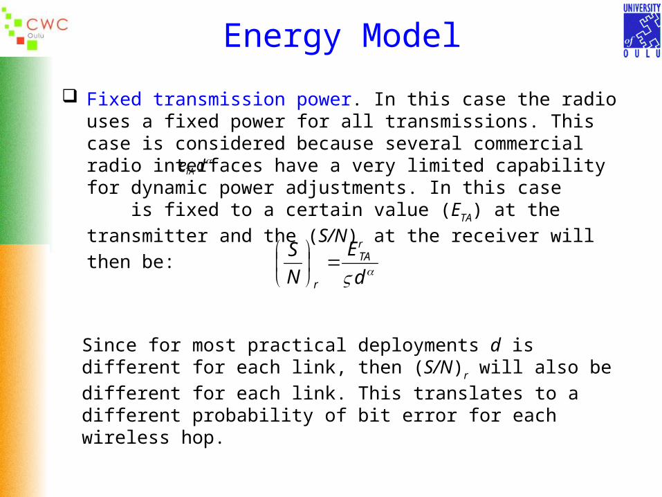
Fixed transmission power. In this case the radio uses a fixed power for all transmissions. This case is considered because several commercial radio interfaces have a very limited capability for dynamic power adjustments. In this case is fixed to a certain value (ETA) at the transmitter and the
(S/N)r at the receiver will then be:
deTA
d
E
N
S TA
r
Since for most practical deployments d is different for each link, then (S/N)r will also be different for each link. This translates to a different
probability of bit error for each wireless hop.
Energy Consumption - Multihop Network
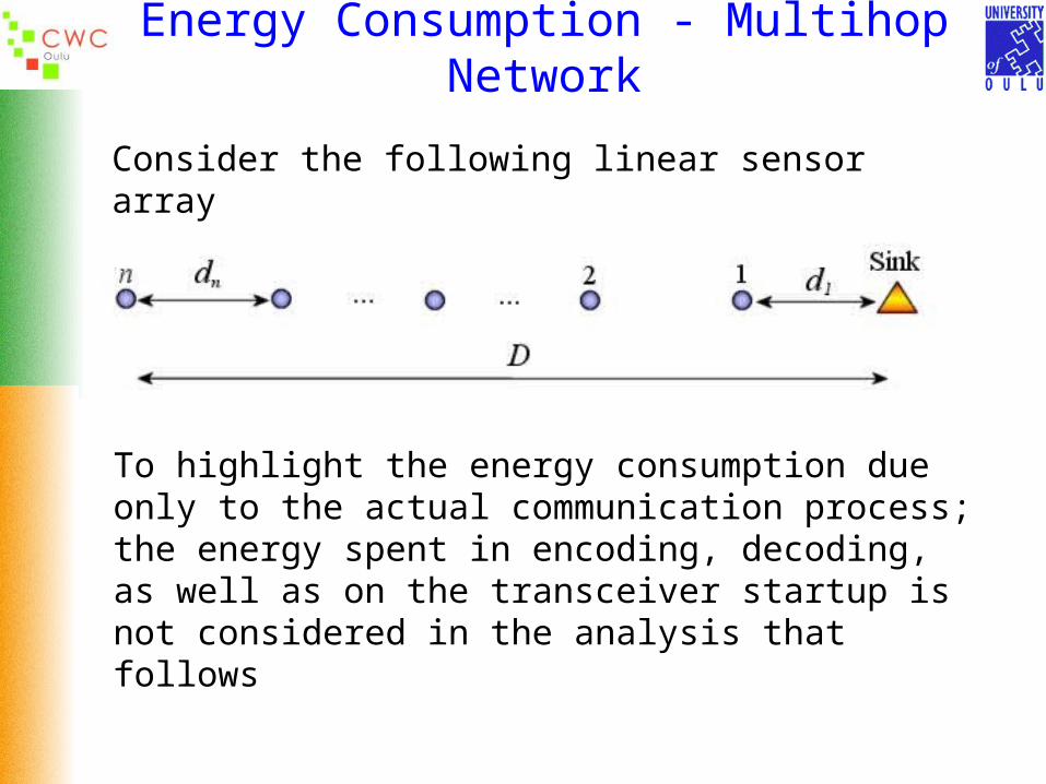
Consider the following linear sensor array
To highlight the energy consumption due only to the actual communication process; the energy spent in encoding, decoding, as well as on the transceiver startup is not considered in the analysis that follows

Energy Consumption - Multihop Networks
The initial assumption is that there is one data packet being relayed from the node farthest from the sink node towards the sink. The total energy consumed by the linear array to relay a packet of m bits from node n to the sink is:
It then can be shown that Elinear is minimum when all the distances
di’s are made equal to D/n, i.e. all the distances are equal.
)()( 12
deedeeemE TATC
n
iiTARCTClinear

Energy Consumption - Multihop Networks
It can also be shown that the optimal number of hops is,
charcharopt d
D
d
Dn or
where
1
)1(
TA
RCTCchar e
eed
dchar depends only on the path loss exponent α and on the transceiver hardware dependent parameters. Replacing the value of dchar in the expression for Elinear
RC
RCTCoptoptlinear e
eenmE
1
)(
Energy Consumption - Multihop Networks
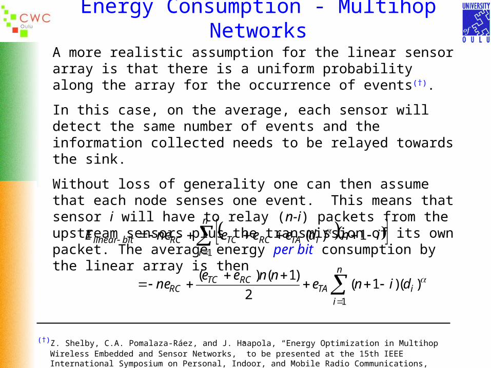
A more realistic assumption for the linear sensor array is that there is a uniform probability along the array for the occurrence of events(†).
In this case, on the average, each sensor will detect the same number of events and the information collected needs to be relayed towards the sink.
Without loss of generality one can then assume that each node senses one event. This means that sensor i will have to relay (n-i) packets from the upstream sensors plus the transmission of its own packet. The average energy per bit consumption by the linear array is then
)()1(2
)1()(
1)(
1
1
i
n
iTA
RCTCRC
n
iiTARCTCRCbitlinear
dinennee
ne
indeeeneE
(†)Z. Shelby, C.A. Pomalaza-Ráez, and J. Haapola, “Energy Optimization in Multihop Wireless Embedded and Sensor Networks,” to be presented at the 15th IEEE International Symposium on Personal, Indoor, and Mobile Radio Communications, September 5-8, 2004, Barcelona, Spain.
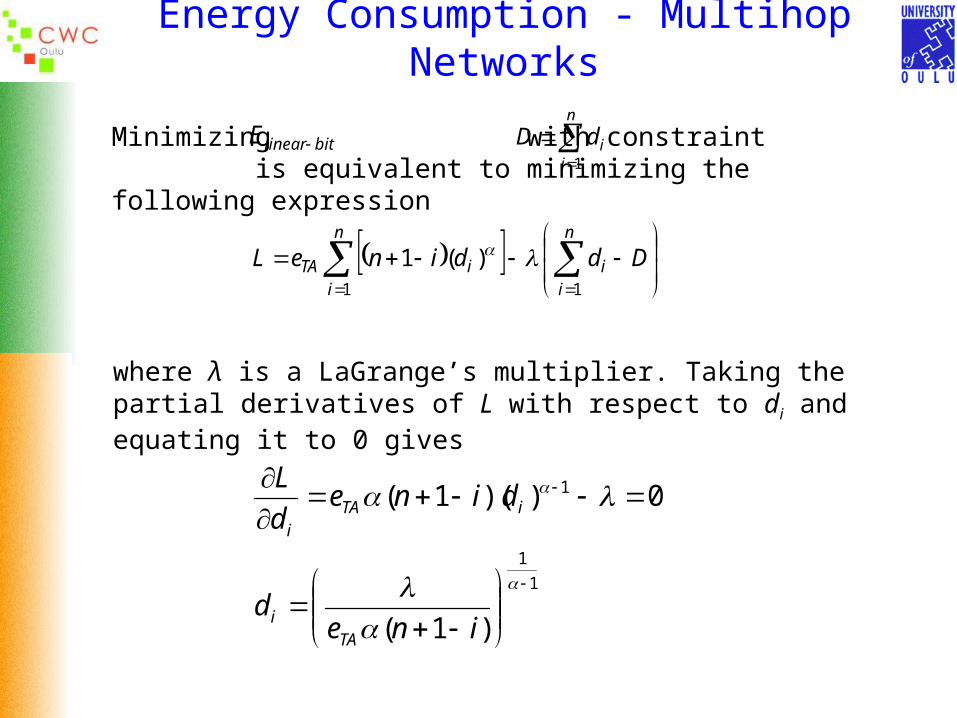
Energy Consumption - Multihop Networks
bitlinearE
n
iidD
1
Minimizing with constraint is equivalent to minimizing the following expression
DddineLn
ii
n
iiTA
11
)(1
where λ is a LaGrange’s multiplier. Taking the partial derivatives of L with respect to di and equating it to 0 gives
1
1
1
)1(
0))(1(
ined
dined
L
TAi
iTAi
Energy Consumption - Multihop Networks
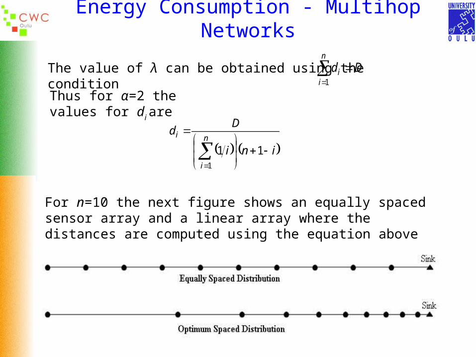
The value of λ can be obtained using the condition
n
ii Dd
1
Thus for α=2 the values for di are
ini
Dd
n
i
i
111
For n=10 the next figure shows an equally spaced sensor array and a linear array where the distances are computed using the equation above (α=2)
Energy Consumption - Multihop Networks
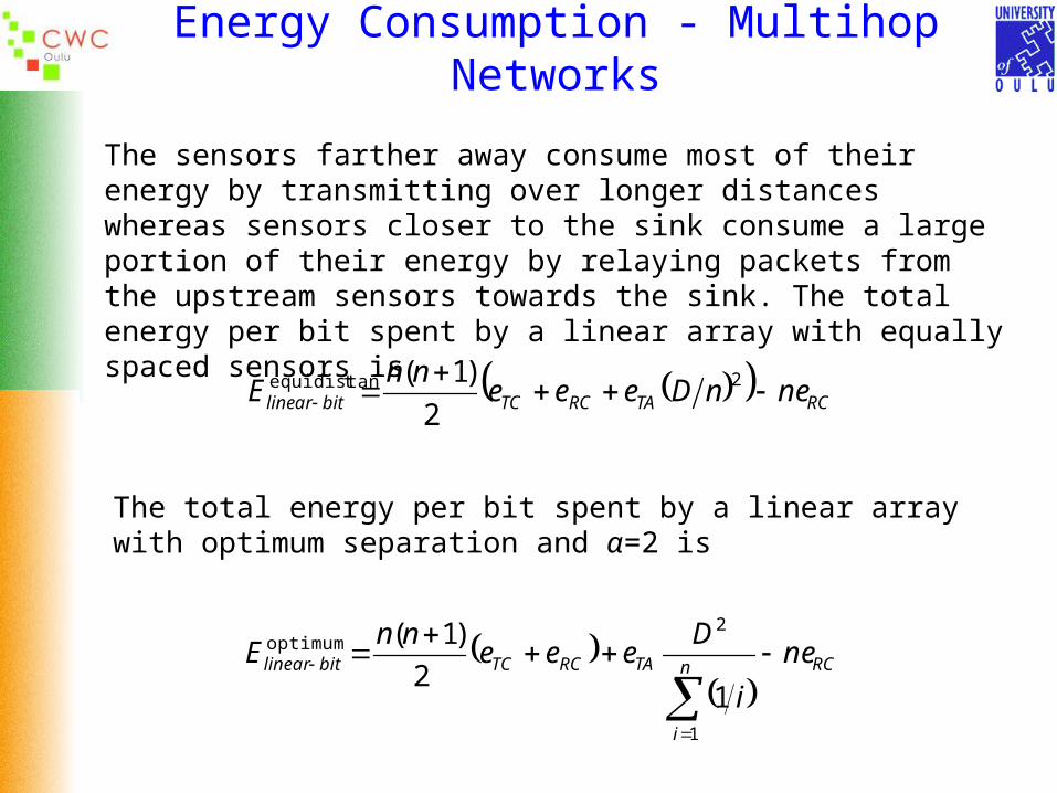
The sensors farther away consume most of their energy by transmitting over longer distances whereas sensors closer to the sink consume a large portion of their energy by relaying packets from the upstream sensors towards the sink. The total energy per bit spent by a linear array with equally spaced sensors is
RCTARCTCbitlinear nenDeeenn
E
2tequidistan
2
)1(
The total energy per bit spent by a linear array with optimum separation and α=2 is
RCn
i
TARCTCbitlinear ne
i
Deee
nnE
1
2optimum
12
)1(
Energy Consumption - Multihop Networks
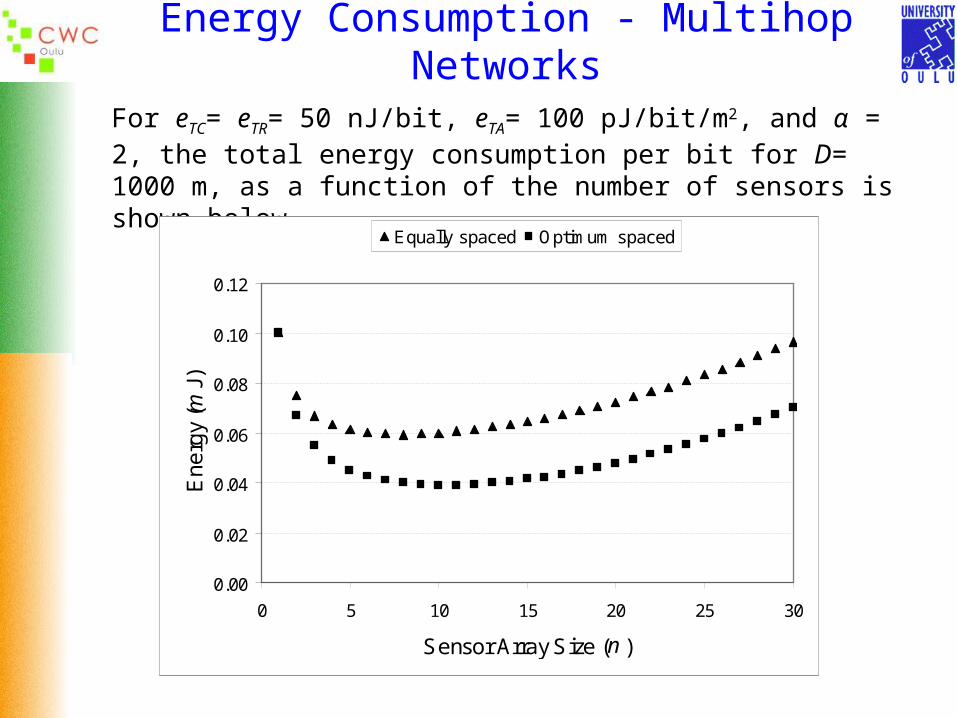
For eTC= eTR= 50 nJ/bit, eTA= 100 pJ/bit/m2, and α = 2, the total energy consumption per bit for D= 1000 m, as a function of the number of sensors is shown below.
0.00
0.02
0.04
0.06
0.08
0.10
0.12
0 5 10 15 20 25 30
Sensor Array Size (n )
En
erg
y (m
J)
Equally spaced Optimum spaced

Energy Consumption - Multihop Networks
The energy per bit consumed at node i for the linear arrays discussed can be computed using the following equation. It is assumed that each node relays packets from the upstream nodes towards the sink node via the closest downstream neighbor. For simplicity’s sake only one transmission is used, e.g. no ARQ type mechanism
])())(1[()( RCiTATClinear eindeeiniE
0.0
2.0
4.0
6.0
8.0
0 5 10 15 20
Distance (hops) from the sink
En
erg
y (u
J)
Equally Spaced Optimum Spaced
Total Energy=72.5 uJ
Total Energy = 47.8 uJ
Energy consumption at each node (n=20, D=1000 m)

Data Link Layer
Medium Access Control (MAC)
Lets multiple radios share the same communication media Time
Code
Frequ
ency
Physical
Data Link
Network
Transport
ApplicationResponsible for the multiplexing of the data stream, data frame detection, medium access and error control. Ensures reliable point-to-point and point-to-multipoint connections in a communication network
MAC protocols for sensor networks must have built-in power conservation mechanisms and strategies for the proper management of node mobility or failure

Wireless MAC Protocols
Wireless MAC protocols
DistributedMAC protocols
CentralizedMAC protocols
Randomaccess
Randomaccess
Guaranteedaccess
Hybridaccess
Since it is desirable to turn off the radio as much as possible in order to conserve energy some type of TDMA mechanism is often suggested for WSN applications
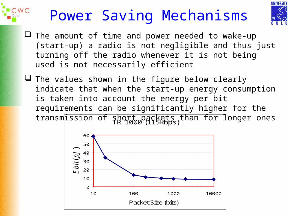
Power Saving Mechanisms The amount of time and power needed to wake-up (start-up) a radio is not
negligible and thus just turning off the radio whenever it is not being used is not necessarily efficient
The values shown in the figure below clearly indicate that when the start-up energy consumption is taken into account the energy per bit requirements can be significantly higher for the transmission of short packets than for longer ones
TR 1000 (115kbps)
0
10
20
30
40
50
60
10 100 1000 10000
Packet Size (bits)
Eb
it ( p
J )

Error ControlError control is an important issue in any radio link
Forward Error Correction (FEC) Automatic Repeat Request (ARQ)
With FEC one pays an a priori battery power consumption overhead and packet delay by computing the FEC code and transmitting the extra code bits.
With ARQ one gambles that the packet will get through and if it does not one has to pay battery energy and delay due to the retransmission process.
Whether FEC or ARQ or a hybrid error control system is energy efficient will depend on the channel conditions and the network requirements such as throughput and delay.
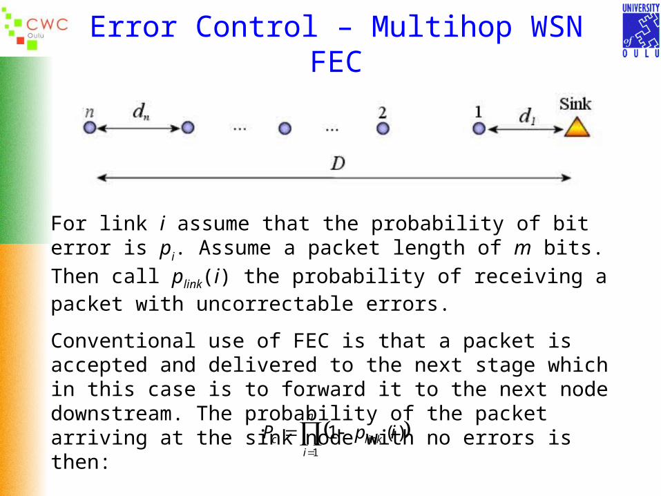
Error Control – Multihop WSNFEC
For link i assume that the probability of bit error is pi. Assume a packet
length of m bits. Then call plink(i) the probability of receiving a packet with uncorrectable errors.
Conventional use of FEC is that a packet is accepted and delivered to the next stage which in this case is to forward it to the next node downstream. The probability of the packet arriving at the sink node with no errors is then:
n
ilinkc ipP
1
)(1
Error Control – Multihop WSN
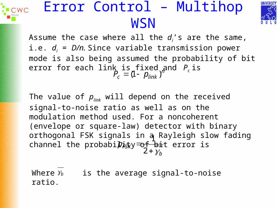
Assume the case where all the di’s are the same, i.e. di = D/n. Since variable transmission power mode is also being assumed the probability of bit error for each link is fixed and Pc is
nlinkc pP )1(
The value of plink will depend on the received signal-to-noise ratio as well
as on the modulation method used. For a noncoherent (envelope or square-law) detector with binary orthogonal FSK signals in a Rayleigh slow fading channel the probability of bit error is
bFSKp
2
1
Where is the average signal-to-noise ratio.b

Error Control – Multihop WSN
Consider a linear code (m, k, d ) is being used. For FSK-modulation with non-coherent detection and assuming ideal interleaving the probability of a code word being in error is bounded by
min
2
2
12
d
b
M
i i
i
M
w
w
P
where wi is the weight of the ith code word and M=2k
Error Control – Multihop WSNA simpler bound for PM is:
min)]1(4)[1( dFSKFSKM ppMP
For the multihop scenario being discussed here plink = PM and the probability of packet error can be written as:
ndFSKFSK
k
nM
nlinkce
pp
PpPP
})]1(4)[12(1{1
)1(1)1(11
min
The probability of successful transmission of a single code word is
)1( esuccess PP

Error Control – Multihop WSN
Parameter Value
NFRx 10dB
N0 -173.8 dBm/Hz or 4.17 * 10-21 J
Rbit 115.2 Kbits
0.3 m
Gant -10dB or 0.1
amp 0.2
3
BW For FSK-modulation, it is assumed to be the same as Rbit
eRC 50nJ/bit
eTC 50nJ/bit
Radio parameters used to obtain the results shown in the next slides

Error Control – Multihop WSN
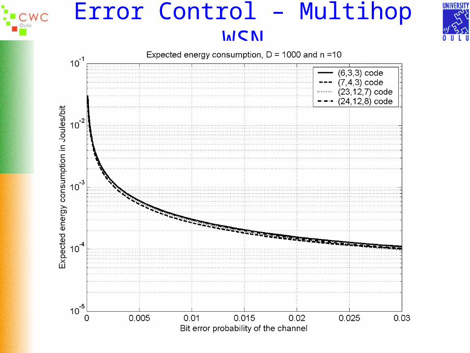
The expected energy consumption per information bit is defined as:
success
linearbitilinear Pk
EE
Parameters for the studied codes are shown in the table below, t is the error correction capability.
Code m k dmin Code rate t
Hamming 7 4 3 0.57 1
Golay 23 12 7 0.52 3
Shortened Hamming
6 3 3 0.5 1
Extended Golay
24 12 8 0.5 3
Error Control – Multihop WSN
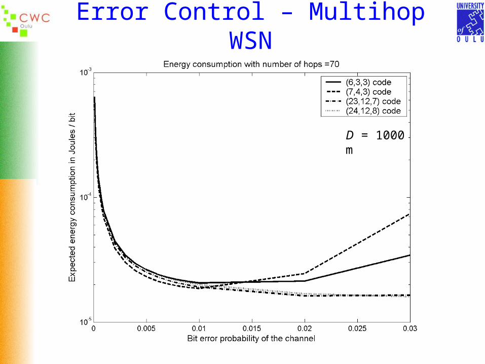
Error Control – Multihop WSN
D = 1000 m
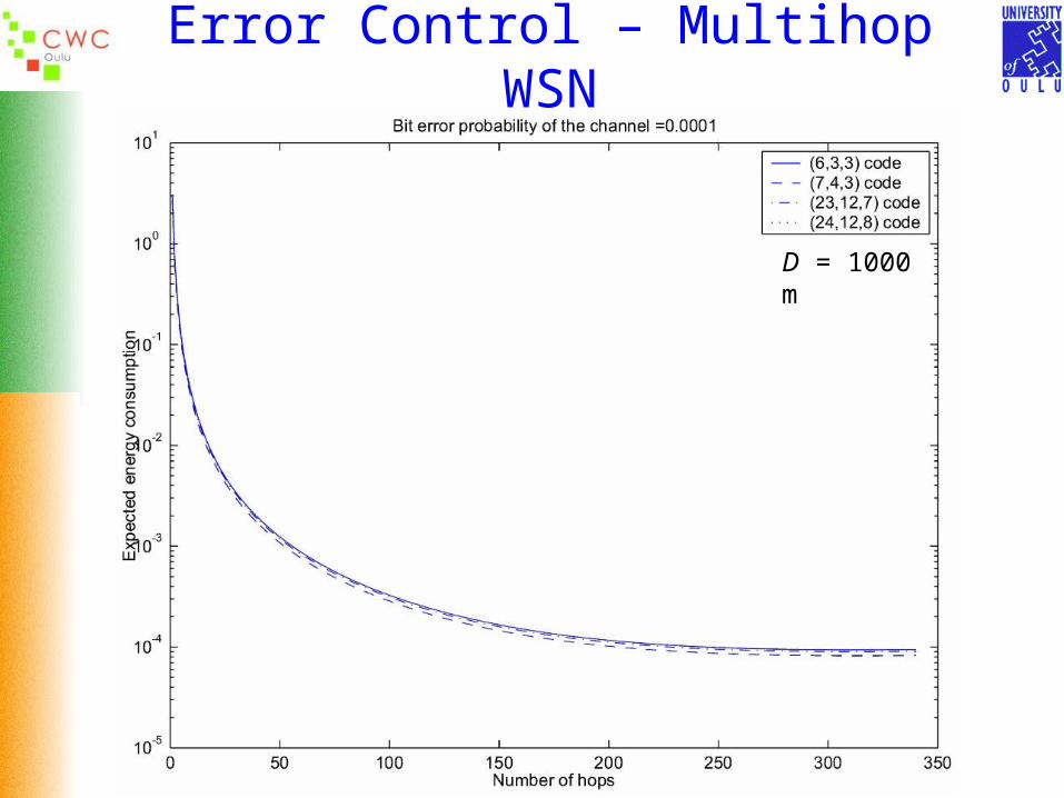
Error Control – Multihop WSN
D = 1000 m

Error Control – Multihop WSN
D = 1000 m
Cooperative Communications inWireless Sensor Networks
Diversity techniques have been proposed and developed to minimize the errors in reception when the channel attenuation is large
In frequency diversity the same information is transmitted on L carriers, where the separation between successive carriers equals or exceeds the coherence bandwidth of the channel
In time diversity the same information is transmitted in L different time slots, where the separation between successive time slots equals or exceeds the coherence time of the channel
In space, or multi-antenna diversity the antennas are sufficiently far apart that the multipath components of the signal have different propagation delays so they fade independently
Unlike conventional space diversity techniques that rely on antenna arrays at the transmitter or receiver terminal the cooperative communications discussed here assume that each node has its own information to transmit and has one antenna. The terminals cooperate, i.e. share their antennas and other resources, to create a “virtual array”

Cooperative Communications
T1
T2
T3
T4
T1 and T2 transmit to terminals T3 and T4 T1 and T2 can listen to each other’s transmission and jointly
communicate their information For sensor networks the objective is to attain an improved
performance, e.g. decreased BER and/or decreased energy consumption
In cooperative mode each user transmits its own bits as well as some information bits from its partners
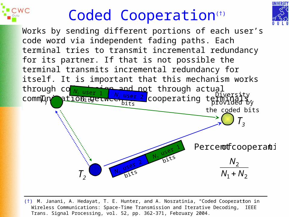
Coded Cooperation(†)
Works by sending different portions of each user’s code word via independent fading paths. Each terminal tries to transmit incremental redundancy for its partner. If that is not possible the terminal transmits incremental redundancy for itself. It is important that this mechanism works through code design and not through actual communication between the cooperating terminals.
T1
T2
T3
N1 user 1 bits N2 user 2 bits
N 2 user 2 bits
N 1 user 1 bits
Diversity provided by the coded bits
21
2
n cooperatio ofPercent
NN
N
(†) M. Janani, A. Hedayat, T. E. Hunter, and A. Nosratinia, “Coded Cooperation in Wireless Communications: Space-Time Transmission and Iterative Decoding,” IEEE Trans. Signal Processing, vol. 52, pp. 362-371, February 2004.
Coded Cooperation
User 1 bits User 2 bits
Rx User 1 bits Idle or sleep User 2 bits User 1 bits
Rx User 2 bits Idle or sleep User 1 bits User 2 bits
Rx User 1 bits Idle or sleep
User 1
User 2time
U1 time slot U2 time slot U1 time slot
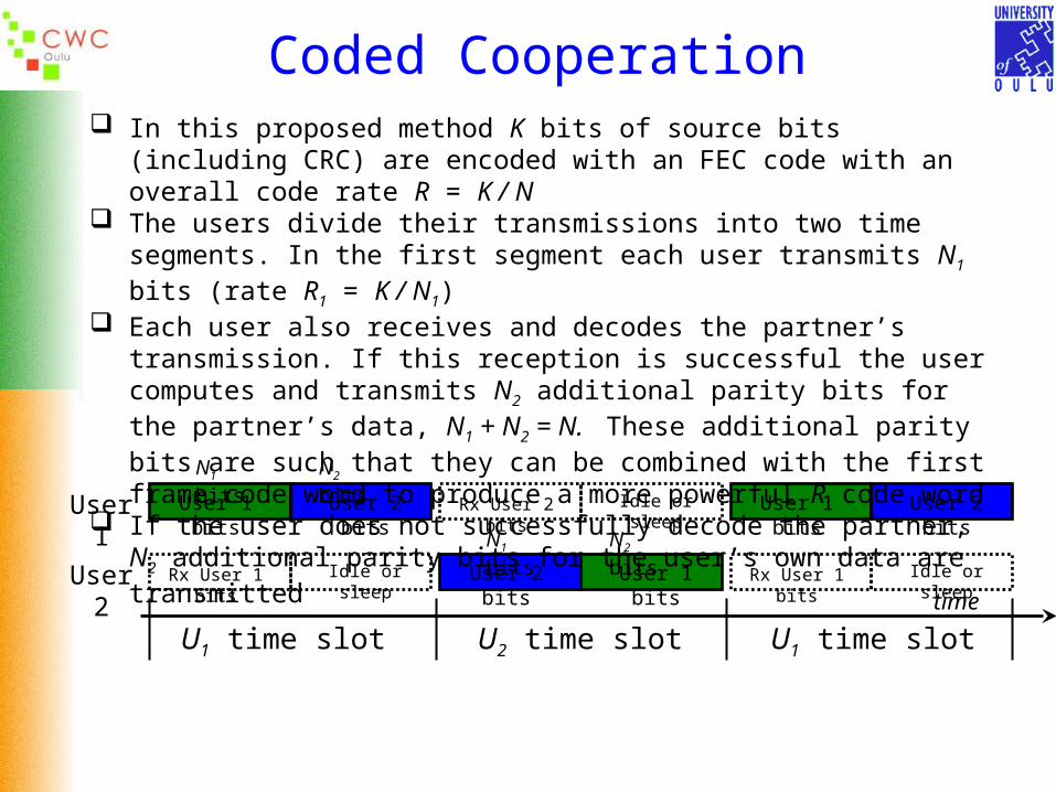
In this proposed method K bits of source bits (including CRC) are encoded with an FEC code with an overall code rate R = K / N
The users divide their transmissions into two time segments. In the first segment each user transmits N1 bits (rate R1 = K / N1)
Each user also receives and decodes the partner’s transmission. If this reception is successful the user computes and transmits N2 additional parity bits for the partner’s data, N1 + N2 = N. These additional parity bits are such that they can be combined with the first frame code word to produce a more powerful R code word
If the user does not successfully decode the partner, N2 additional parity bits for the user’s own data are transmitted
N1 bits N2 bits
N1 bits N2 bits

MAC Protocols for WSNs
Physical
Data Link
Network
Transport
ApplicationWSN protocols have to allow for a closer
collaboration or awareness among the layers of the protocol stack, in particular the first three layers
WSN routing algorithms designed with the concepts of data centric and data aggregation create special requirements on the underlying MAC protocols
These observations can be extended to the design of other layers as well since WSNs call for new networking paradigms
MAC protocols should have the radio transceivers in a sleeping mode as much as possible in order to save energy
Example of a MAC Protocol for WSN
Sensor-MAC (S-MAC)(†) – Is an energy-aware protocol that illustrates design considerations that MAC protocols for WSNs should address. Assumptions made in the design of S-MAC are: Most communications will be between neighboring sensor nodes rather
than between a node and a base station There are many nodes that are deployed in a casual, e.g. not precise,
manner and as such the nodes must be able to self-configure The sensor nodes are dedicated to a particular application and thus per-
node fairness (channel access) is not as important as the application level performance
Since the network is dedicated to a particular application the application data processing can be distributed through the network. This implies that data will be processed as whole messages at a time in store-and-forward fashion allowing for the application of data aggregation techniques which can reduce the traffic
The application can tolerate latency and has long idle periods
Data Link
(†) W. Ye, J. Heidemann and D. Estrin, “An Energy-Efficient MAC Protocol for Wireless Sensor Networks,” In Proceedings of the 21st International Annual Joint Conference of the IEEE Computer and Communications Societies (INFOCOM 2002), New York, NY, USA, June, 2002, pp. 1-10.

Sensor-MAC (S-MAC) The main features of S-MAC are: Periodic listen and sleep Collision and overhearing avoidance Message passing
The basic scheme for each node is:
Each node goes into periodic sleep mode during which it switches the radio off and sets a timer to awake later
When the timer expires it wakes up and listens to see if any other node wants to talk to it
The duration of the sleep and awake cycles are application dependent and they are set the same for all nodes
Requires a periodic synchronization among nodes to take care of any type of clock drift
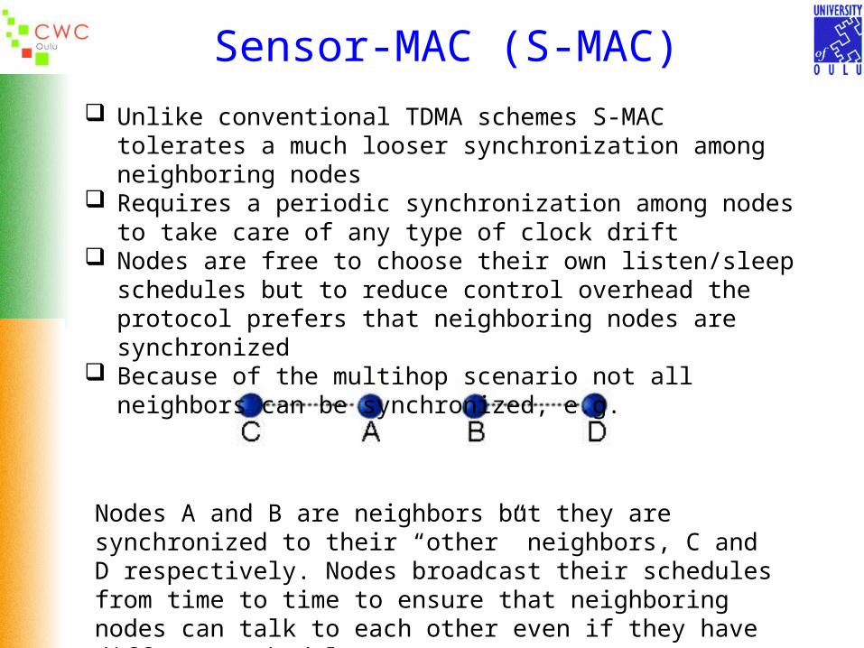
Sensor-MAC (S-MAC) Unlike conventional TDMA schemes S-MAC tolerates a much looser
synchronization among neighboring nodes Requires a periodic synchronization among nodes to take care of any
type of clock drift Nodes are free to choose their own listen/sleep schedules but to
reduce control overhead the protocol prefers that neighboring nodes are synchronized
Because of the multihop scenario not all neighbors can be synchronized, e.g.
Nodes A and B are neighbors but they are synchronized to their “other” neighbors, C and D respectively. Nodes broadcast their schedules from time to time to ensure that neighboring nodes can talk to each other even if they have different schedules

Sensor-MAC (S-MAC)Choosing and Maintaining Schedules Each node maintains a schedule table that stores schedules of all its
known neighbors To establish the initial schedule the following steps are followed:
A node first listens for a certain amount of time If it does not hear a schedule from another node, it randomly
chooses a schedule and broadcasts its schedule immediately This node is called a Synchronizer If a node receives a schedule from a neighbor before choosing its
own schedule, it just follows this neighbor’s schedule, i.e. becomes a Follower and it waits for a random delay and broadcasts its schedule
If a node receives a neighbor’s schedule after it selects its own schedule, it adopts both schedules and broadcasts its own schedule before going to sleep
It is expected that very rarely a node adopts multiple schedules since every node tries to follow existing schedules before choosing an independent one

Sensor-MAC (S-MAC)
Maintaining Synchronization Timer synchronization among neighbors is needed to prevent clock drift.
The updating period can be relatively long (tens of seconds) Done by periodically sending a SYNC packet that only includes the
address of the sender and the time of its next sleeping period Time of next sleep is relative to the moment that the sender finishes
transmitting the SYNC packet A node will go to sleep when the timer fires Receivers will adjust their timer counters immediately after they receive
the SYNC packet A node periodically broadcasts a SYNC packet to its neighbors even if it
has no followers

Sensor-MAC (S-MAC)
Maintaining Synchronization (cont.)
Listen interval is divided into two parts: one for receiving SYNC packets and the other for receiving RTS (Request To Send)
Sensor-MAC (S-MAC)Collision and Overhearing Avoidance Similar to IEEE 802.11, i.e. uses RTS/CTS mechanism to address the
hidden terminal problem Performs carrier sense before initiating a transmission If a node fails to get the medium, it goes to sleep and wakes up when the
receiver is free and listening again Duration field in each transmitted packet indicates how long the
remaining transmission will be, so if a node receives a packet destined for another node, it knows how long it has to keep silent
The node records this value in the network allocation vector (NAV) and sets a timer for it
When a node has data to send, it first looks at NAV. If this value is not zero, then the medium is busy (virtual carrier sense)
The medium is determined as free if both the virtual and physical carrier sense indicate the medium is free
All immediate neighbors of both the sender and receiver should sleep after they hear the RTS or CTS packet until the current transmission is over
Sensor-MAC (S-MAC)Message Passing A message is a collection of meaningful, interrelated units of data Transmitting a long message as a packet is disadvantageous as the re-
transmission cost is high if the packet is corrupted Fragmentation into small packets will lead to high control overhead as
each packet should contend using RTS/CTS S-MAC fragments message into small packets and transmits them as a
burst Only one RTS packet and one CTS packets are used Every time a data fragment is transmitted the sender waits for an ACK
from the receiver. If it does not arrive the fragment is retransmitted and the reservation is extended for the duration of the fragment
Advantages: Reduces latency of the message Reduces control overhead
Disadvantage: Node-to-node fairness is reduced, as nodes with small packets to
send will have to wait until the message burst is transmitted
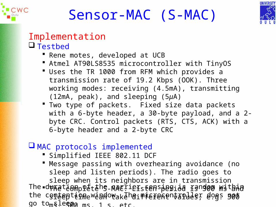
Sensor-MAC (S-MAC)Implementation Testbed
Rene motes, developed at UCB Atmel AT90LS8535 microcontroller with TinyOS Uses the TR 1000 from RFM which provides a transmission rate of 19.2
Kbps (OOK). Three working modes: receiving (4.5mA), transmitting (12mA, peak), and sleeping (5μA)
Two type of packets. Fixed size data packets with a 6-byte header, a 30-byte payload, and a 2-byte CRC. Control packets (RTS, CTS, ACK) with a 6-byte header and a 2-byte CRC
MAC protocols implemented Simplified IEEE 802.11 DCF Message passing with overhearing avoidance (no sleep and listen
periods). The radio goes to sleep when its neighbors are in transmission The complete S-MAC. Listen period is 300 ms and sleep time can take
different values, e.g. 300 ms, 500 ms, 1 s, etc.
The duration of the carrier sensing is random within the contention window. The microcontroller does not go to sleep.

Sensor-MAC (S-MAC)
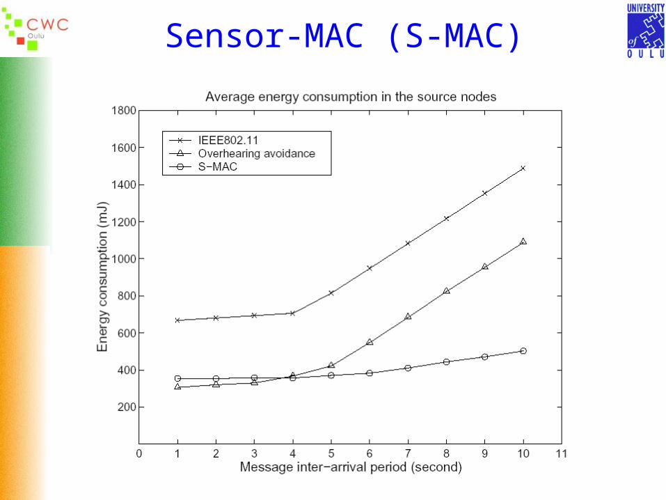
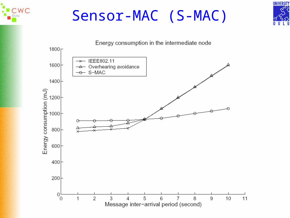
Topology Two-hop network with two sources and two sinks Sources periodically generate a sensing message which is divided
into fragments Traffic load is changed by varying the inter-arrival period of the
messages
Sensor-MAC (S-MAC)

Sensor-MAC (S-MAC)
Sensor-MAC (S-MAC)
Sensor-MAC (S-MAC)
Conclusion The S-MAC protocol has good energy conserving properties when
compared with the IEEE 802.11 standard
Comments Need of a mathematical analysis Need to study the effect of different topologies Fragmenting long packets into smaller ones is not energy efficient. The
argument about more chances of the packet being corrupted is not correct unless other options such as the use of error control coding have also been explored
Several features behind the S-MAC protocol are still “captured” in the traditional way to do business at the Link Layer level, e.g. use of RTS/CTS/ACK, etc.
The protocol does not address the fact that in most sensor net applications neighboring nodes are activated almost at the same time by the event to be sensed and as such they will attempt to communicate at approximately the same time. There is also a high degree of correlation between the data they want to communicate

Network Layer
Physical
Data Link
Network
Transport
Application
Basic issues :
Power efficiency Data centric – The nature of the data determines
the traffic flow Data aggregation – To manage the potential
implosion of traffic because of the data centric routing
Rather than conventional node addresses, use attribute-based addressing, e.g. “region where humidity is below 5%”
Locationing systems, i.e. ability of the nodes to establish position information
Internetworking with external networks via gateway or proxy nodes
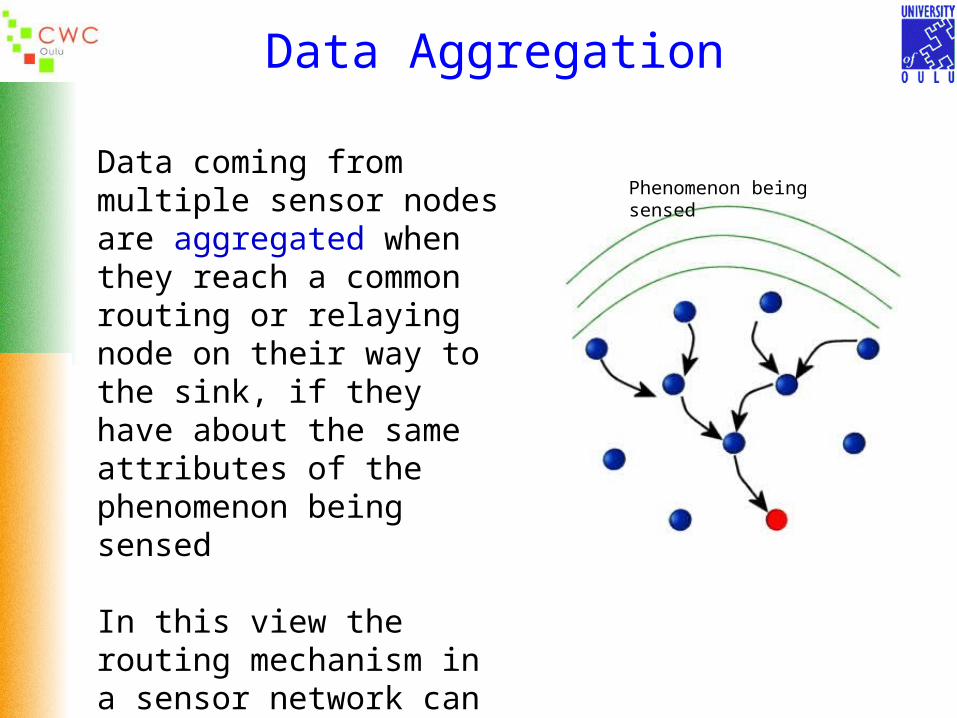
Data Aggregation
Data coming from multiple sensor nodes are aggregated when they reach a common routing or relaying node on their way to the sink, if they have about the same attributes of the phenomenon being sensed
In this view the routing mechanism in a sensor network can be considered as a form of reverse multicast tree
Phenomenon being sensed
Data Centrality
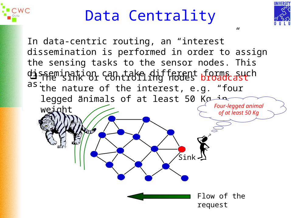
In data-centric routing, an “interest ” dissemination is performed in order to assign the sensing tasks to the sensor nodes. This dissemination can take different forms such as:
The sink or controlling nodes broadcast the nature of the interest, e.g. “four legged animals of at least 50 Kg in weight”
Sink
Four-legged animal of at least 50 Kg
Flow of the request
Data Centrality
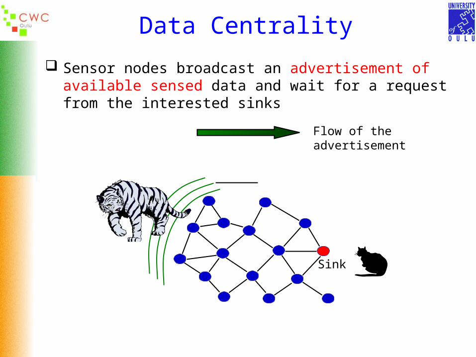
Sensor nodes broadcast an advertisement of available sensed data and wait for a request from the interested sinks
Sink
Flow of the advertisement
Routing
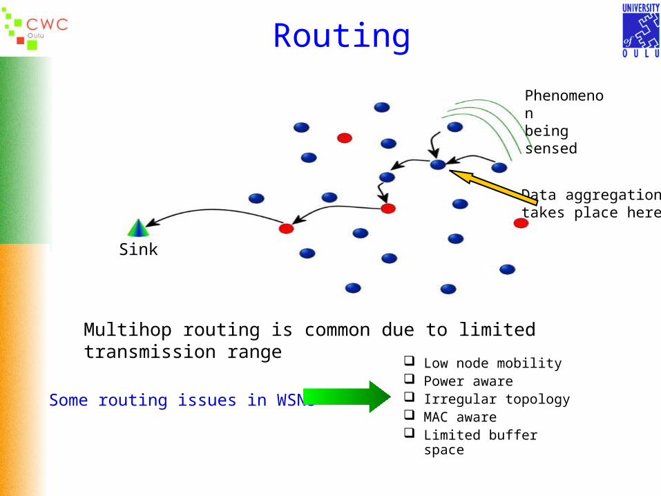
Multihop routing is common due to limited transmission range
Phenomenonbeing sensed
Sink
Low node mobility Power aware Irregular topology MAC aware Limited buffer space
Some routing issues in WSNs
Data aggregationtakes place here
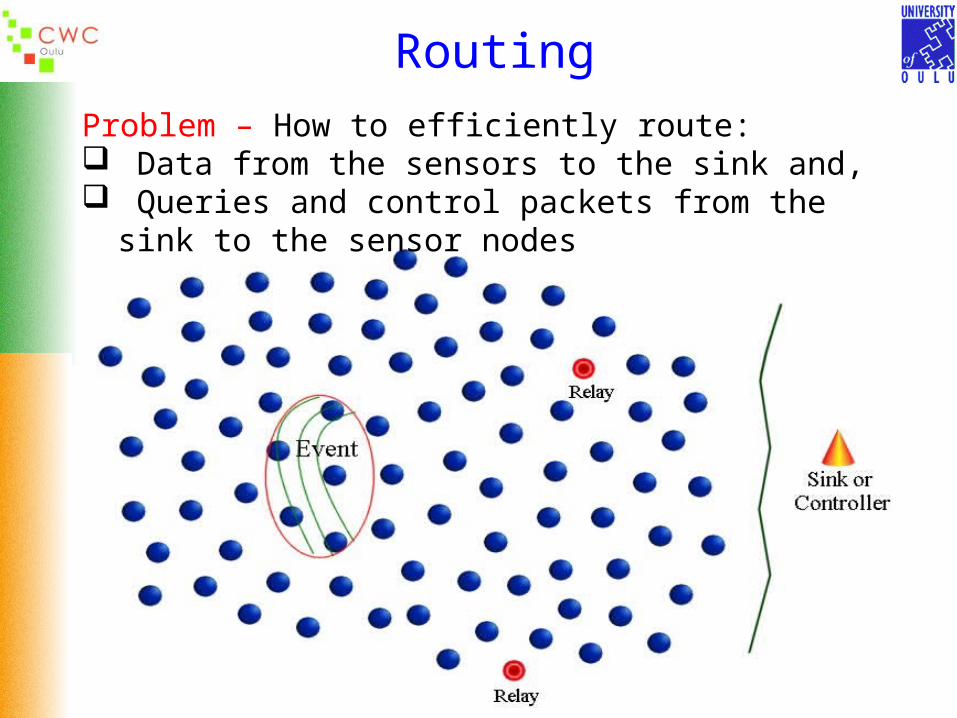
RoutingProblem – How to efficiently route: Data from the sensors to the sink and, Queries and control packets from the sink to the sensor nodes

Routing
In addition to the concepts of data aggregation and data centrality, it is important to identify the nature of the WSN traffic, which will depend on the application.
Assuming a uniform density of nodes, the number of transmissions can be used as a metric for energy consumption.
Since receiving a packet consumes almost as much energy as transmitting a packet it is also important that the MAC protocol limits the number of listening neighbors in order to conserve energy.
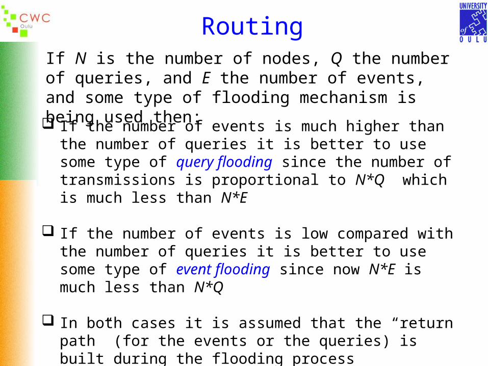
RoutingIf N is the number of nodes, Q the number of queries, and E the number of events, and some type of flooding mechanism is being used then:
If the number of events is much higher than the number of queries it is better to use some type of query flooding since the number of transmissions is proportional to N*Q which is much less than N*E
If the number of events is low compared with the number of queries it is better to use some type of event flooding since now N*E is much less than N*Q
In both cases it is assumed that the “return path” (for the events or the queries) is built during the flooding process
Other underlying routing mechanisms are recommended if the number of events and queries are of the same order
Proposed Routing Techniques
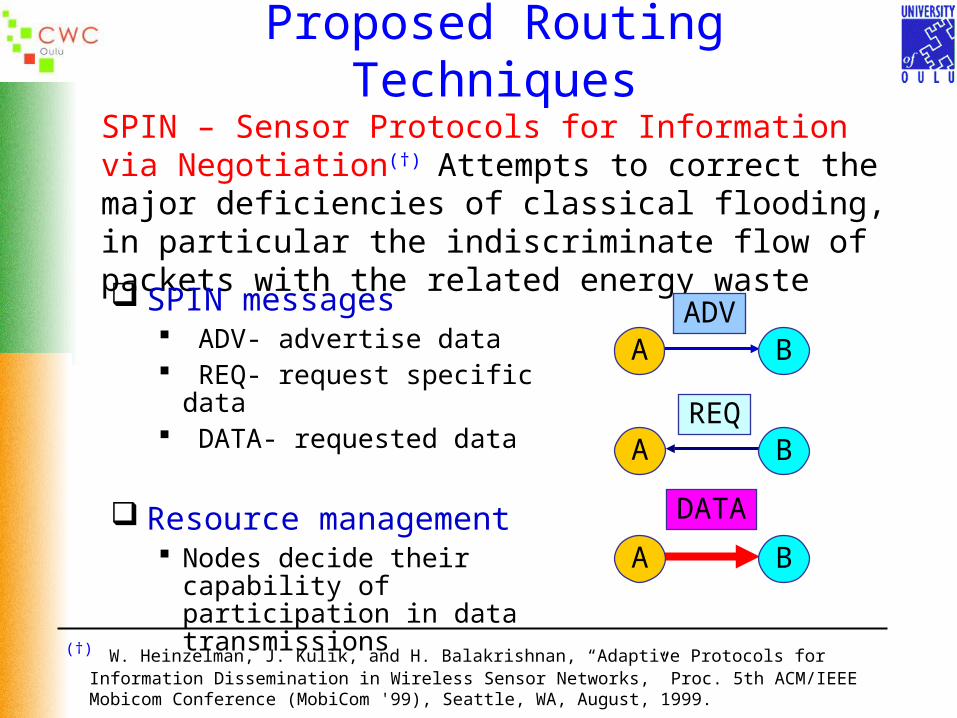
SPIN – Sensor Protocols for Information via Negotiation(†)
Attempts to correct the major deficiencies of classical flooding, in particular the indiscriminate flow of packets with the related energy waste
SPIN messages ADV- advertise data REQ- request specific data DATA- requested data
Resource management Nodes decide their capability of
participation in data transmissions
A B
A B
A B
ADV
REQ
DATA
(†) W. Heinzelman, J. Kulik, and H. Balakrishnan, “Adaptive Protocols for Information Dissemination in Wireless Sensor Networks,” Proc. 5th ACM/IEEE Mobicom Conference (MobiCom '99), Seattle, WA, August, 1999.
SPIN
A mechanism developed for the case where the number of queries is higher than the number of events. Use information descriptors or meta-data for negotiation prior to
transmission of the data Each node has its own energy resource manager which is used to adjust
its transmission activity The family of SPIN protocols are:
SPIN-PP – For point-to-point communication SPIN-EC – Similar to SPIN-PP but with energy conservation
heuristics added to it SPIN-BC – Designed for broadcast networks. Nodes set random
timers after receiving ADV and before sending REQ to wait for someone else to send the REQ
SPIN-RL – Similar to SPIN-BC but with added reliability. Each node keeps track of whether it receives requested data within the time limit, if not, data is re-requested

A node senses something “interesting”Neighbor sends a REQ listing all of the data it would like to acquireSensor broadcasts dataNeighbors aggregate data and broadcast(advertise) meta-data
SPIN-BC
The process repeats itself across the network
DATAREQADV
It sends meta-data to neighbors

SPIN-BC
I am tired I need to sleep …
Advertise meta-data
Request data
Send dataAdvertise
Advertise
Nodes do need not to participate in the process
Request data
Send data
Send data
Advertise meta-data
Request data
Send data
SPIN
Pros Energy – More efficient than flooding Latency – Converges quickly Scalability – Local interactions only Robust – Immune to node failures
Cons Nodes always participating It does not propose the type of MAC layer needed to
support an efficient implementation of this protocol. The simulation analysis uses a modified 802.11 MAC protocol

Directed Diffusion(†)
A mechanism developed for the case where it is expected that the number of events is higher than the number of queries Is data-centric in nature The sink propagates its queries or “interests” in the form of attribute-
value pairs The interests are injected by the sink and disseminated throughout the
network. During this process, “gradients” are set at each sensor that receives an interest pointing towards the sensor from which the interest was received
This process can create, at each node, multiple gradients towards the sink. To avoid excessive traffic along multiple paths a “reinforcement” mechanism is used at each node after receiving data, e.g. reinforce: Neighbor from whom new events are received Neighbor who is consistently performing better than others Neighbor from whom most events received
There is also a mechanism of “negative reinforcement” to degrade the importance of a particular path
(†) C. Intanagonwiwat, R. Govindan, and D. Estrin, “Directed Diffusion: A Scalable and Robust Communication Paradigm for Sensor Networks,” Proc. ACM Mobicom, Boston, MA, August 2000, pp. 1-12.
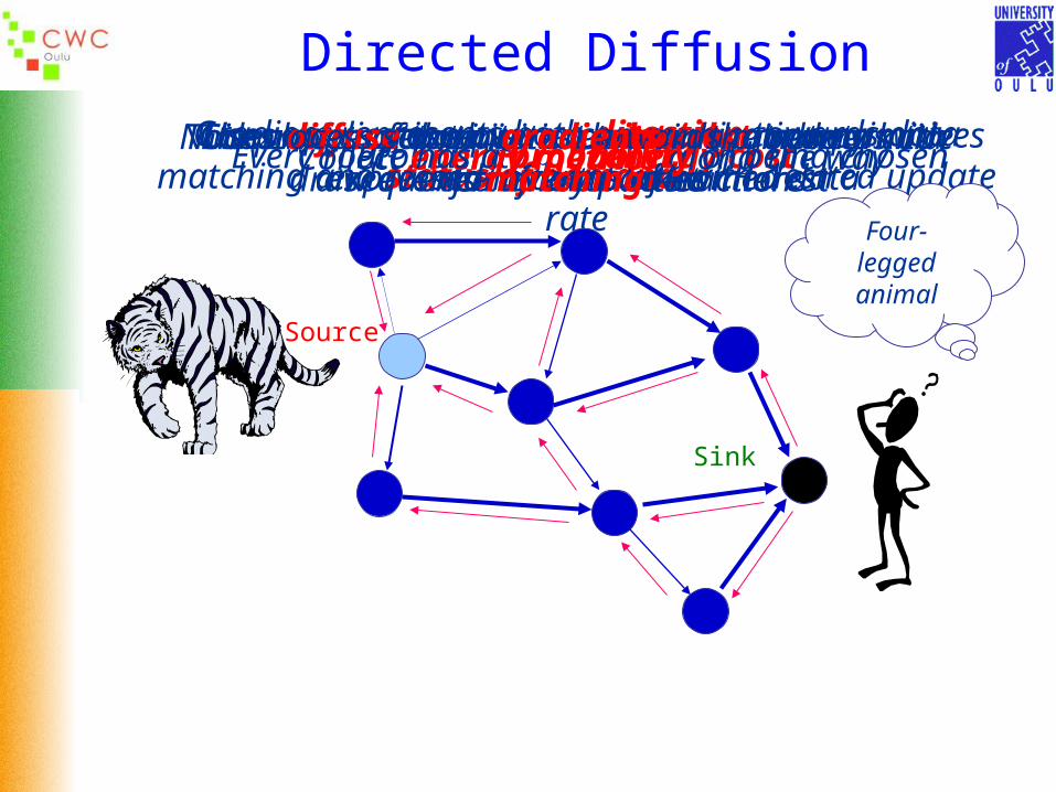
Gradient represents both direction towards data matching and status of demand with desired update rate
Probability 1/energy costThe choice of path is made locally at every node for every packet
Uses application-aware communication primitivesexpressed in terms of named data
Consumer of data initiates interest in data with certain attributes
Nodes diffuse the interest towards producers via a sequence of local interactions
This process sets up gradients in the network to draw events matching the interest
Collect energy metrics along the wayEvery route has a probability of being chosen
Directed Diffusion
Sink
Source
Four-leggedanimal

Reinforcement and negative reinforcement used to converge to efficient distribution
Has built-in tolerance to nodes moving out of range or dying
Directed Diffusion
Source
Sink

Directed Diffusion
Pros Energy – Much less traffic than flooding. For a network of
size N the total cost of transmissions and receptions is whereas for flooding the order is
Latency – Transmits data along the best path Scalability – Local interactions only Robust – Retransmissions of interests
Cons The set up phase of the gradients is expensive It does not propose the type of MAC layer needed to support
an efficient implementation of this protocol. The simulation analysis uses a modified 802.11 MAC protocol
)( NnO)(nNO

Other Proposed Routing Techniques
Data Funneling(†) – Attempts to minimize the amount of communication from the sensors to the information consumer node (sink). It facilitates data aggregation and tries to concentrate the packet flow into a single stream from the group of sensors to the sink.
Controller divides the sensing area into regions
Controller performs a directional flood towards each region
When the packet reaches the region the first receiving node becomes a border node and modifies the packet (adds fields) for route cost estimations within the region
The border node flood the region with modified packet
Sensor nodes in the region use cost information to schedule which border nodes to use
Setup phase:
(†) D. Petrovic, R. C. Shah, K. Ramchandran, and J. Rabaey, “Data Funneling: Routing with Aggregation and Compression for Wireless Sensor Networks,” SNPA 2003, pp. 1-7.
Data Funneling
When a sensor has data it uses the schedule to choose the border node that is to be used
It then waits for time inversely proportional to the number of hops from the border
Along the way to the border node, the data packets join together until they reach the border node
The border node collects all packets and then sends one packet with all the data back to the controller
Data Communication Phase:
Routing - Summary
In recent years a very large number of routing algorithms for WSNs have been proposed and analyzed
Most of the analysis has been carried out using simulation experiments
The majority of the proposed routing algorithms are not supported by a proper MAC protocol
MAC protocols should also be more in tune with important features of the WSN paradigm, e.g. asymmetric flow, no need to have to use individual node addresses or links, have the radio in sleep mode as much as possible, etc.
An aspect that still needs more research is the impact of error control coding on the consumption of energy
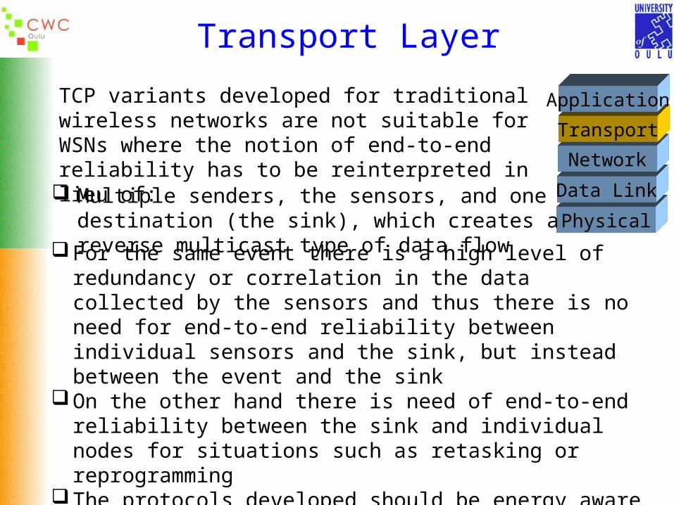
Transport Layer
Physical
Data Link
Network
Transport
ApplicationTCP variants developed for traditional wireless networks are not suitable for WSNs where the notion of end-to-end reliability has to be reinterpreted in lieu of:
Multiple senders, the sensors, and one destination (the sink), which creates a reverse multicast type of data flow
For the same event there is a high level of redundancy or correlation in the data collected by the sensors and thus there is no need for end-to-end reliability between individual sensors and the sink, but instead between the event and the sink
On the other hand there is need of end-to-end reliability between the sink and individual nodes for situations such as retasking or reprogramming
The protocols developed should be energy aware and simple enough to be implemented for the low-end type of hardware and software of many WSN applications
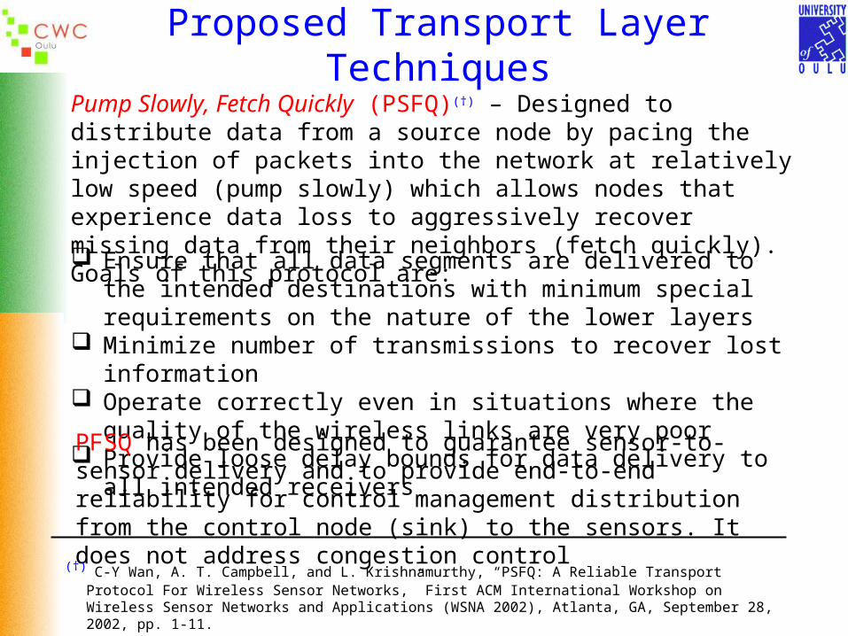
Proposed Transport Layer Techniques
Pump Slowly, Fetch Quickly (PSFQ)(†) – Designed to distribute data from a source node by pacing the injection of packets into the network at relatively low speed (pump slowly) which allows nodes that experience data loss to aggressively recover missing data from their neighbors (fetch quickly). Goals of this protocol are:
Ensure that all data segments are delivered to the intended destinations with minimum special requirements on the nature of the lower layers
Minimize number of transmissions to recover lost information Operate correctly even in situations where the quality of the wireless
links are very poor Provide loose delay bounds for data delivery to all intended receivers
PFSQ has been designed to guarantee sensor-to-sensor delivery and to provide end-to-end reliability for control management distribution from the control node (sink) to the sensors. It does not address congestion control
(†) C-Y Wan, A. T. Campbell, and L. Krishnamurthy, “PSFQ: A Reliable Transport Protocol For Wireless Sensor Networks,” First ACM International Workshop on Wireless Sensor Networks and Applications (WSNA 2002), Atlanta, GA, September 28, 2002, pp. 1-11.

PSFQA transport protocol for WSNs that attempts to pace the data from a source node at a relatively low speed to allow intermediate nodes to fetch missing data segments from their neighbors, e.g. hop-by-hop recovery instead of traditional transport layer end-to-end recovery mechanisms
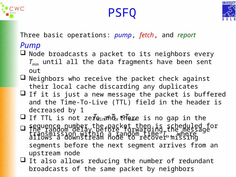
PSFQ
Three basic operations: pump, fetch, and report
Pump Node broadcasts a packet to its neighbors every Tmin until all the data
fragments have been sent out Neighbors who receive the packet check against their local cache
discarding any duplicates If it is just a new message the packet is buffered and the Time-To-Live
(TTL) field in the header is decreased by 1 If TTL is not zero and there is no gap in the sequence number the packet
then is scheduled for transmission within a random time Ttx, wheremaxmin TTT tx
The random delay before forwarding the message allows a downstream node to recover missing segments before the next segment arrives from an upstream node
It also allows reducing the number of redundant broadcasts of the same packet by neighbors
PFSQ
FetchA node goes into fetch mode when a sequence number gap is detected In fetch mode a node aggressively sends out NACK messages to its
immediate neighbors to request missing segments Since it is very likely that consecutive packets are lost because of fading
conditions, a “window” is used to specify the range of missing packets A node that receives a NACK message checks the loss window field
against its cache. If found the packet is scheduled for transmission at a random time in (0, Tr)
Neighbors cancel a retransmission when a reply for the same segment is overheard
NACK messages are not propagated to avoid message implosion There is also a “proactive fetch” mode to take care of situations such as
when the last segment of a message is lost. In this case the node sends a NACK for the remaining segments when they have not been received after a time period Tpro
PFSQ
Report Used to provide feedback data of delivery status to source nodes To minimize the number of messages, the protocol is designed so that a
report message travels back from a target node to the source nodes. Intermediate nodes can also piggyback their report messages in an aggregated manner
Simulation and experimental evaluation When compared to a previously proposed similar protocol (Scalable
Reliable Multicast) the simulation results show that the PFSQ protocol has a better performance in terms of error tolerance, communications overhead, and delivery latency
The experimental results were obtained by using the TinyOS platform on RENE motes. The performance results were much poorer than the simulation results. The discrepancy is attributed to the simulation experiment being unable to accurately model the wireless channel and the computational demands on the sensor node processor
Proposed Transport Layer Techniques
Event-to-Sink Reliable Transport (ESRT) (†) – Designed to achieve reliable event detection (at the sink node) with a protocol that is energy aware and has congestion control mechanisms. Salient features are:Self-configuration – even in the case of a dynamic topologyEnergy awareness – sensor nodes are notified to decrease their frequency of
reporting if the reliability level at the sink node is above the minimumCongestion control – takes advantage of the high level of correlation between the
data flows corresponding to the same eventCollective identification – sink only interested in the collective information from a
group of sensors, not in their individual reports
(†) Y. Sankarasubramaniam, O. B. Akan, and I. F. Akyildiz, “ESRT: Event-to-Sink Reliable Transport in Wireless Sensor Networks” Proceedings of ACM MobiHoc`03, Annapolis, Maryland, USA, June 2003, pp. 177-188.
ESRT In a typical sensor network application the sink node is only interested in
the collective information of the sensor nodes within the region of an event and not in any individual sensor data
Traditional end-to-end reliability requirements do not then apply here What is needed is a measure of the accuracy of the information received at
the sink, i.e. and event-to-sink reliability

The basic assumption is that the sink does all the reliability evaluation using parameters that are application dependent
One such parameter is the decision time interval τ
At the end of the decision interval the sink derives a reliability indicator ri based on the reports received from the sensor nodes
ri is the number of packets received in the decision interval
If R is the number of packets required for reliable event detection then ri > R is needed for reliable event detection
There is no need to identify individual sensor nodes but instead there is the need to have an event ID
The reporting rate, f, of a sensor node is the number of packets sent out per unit time by that node
The ESRT protocol aims to dynamically adjust the reporting rate to achieve the required detection reliability R at the sink
ESRT
ESRT
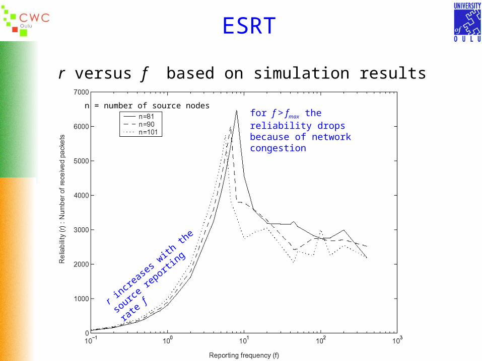
r versus f based on simulation results
n = number of source nodes
r incre
ases w
ith th
e
source
reportin
g rate f
for f > fmax the reliability drops because of network congestion
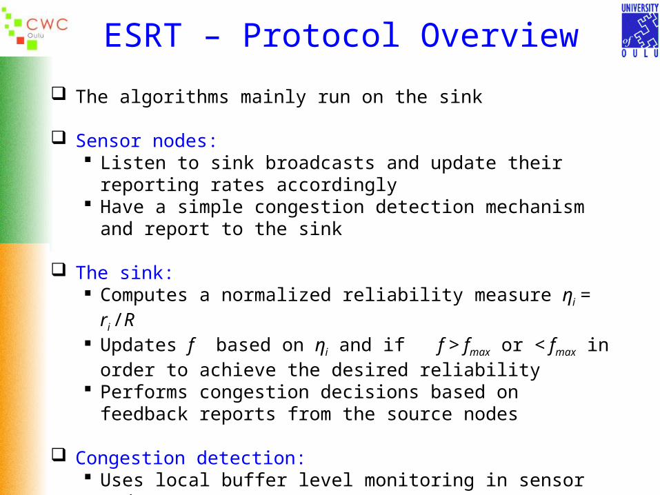
ESRT – Protocol Overview
The algorithms mainly run on the sink
Sensor nodes: Listen to sink broadcasts and update their reporting rates accordingly Have a simple congestion detection mechanism and report to the
sink
The sink: Computes a normalized reliability measure ηi = ri /R Updates f based on ηi and if f > fmax or < fmax in order to achieve the
desired reliability Performs congestion decisions based on feedback reports from the
source nodes
Congestion detection: Uses local buffer level monitoring in sensor nodes When a routing buffer overflows the node informs the sink by
setting the congestion notification bit in the header packets traveling downstream

ESRT – Network States
(No congestion, Low reliability)
(Congestion, Low reliability)
(Congestion, High reliability)
(No congestion, High reliability)
Optimal Operating Region
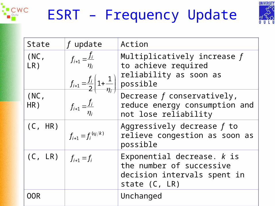
ESRT – Frequency Update
State f update Action
(NC, LR) Multiplicatively increase f to achieve required reliability as soon as possible
(NC, HR) Decrease f conservatively, reduce energy consumption and not lose reliability
(C, HR) Aggressively decrease f to relieve congestion as soon as possible
(C, LR) Exponential decrease. k is the number of successive decision intervals spent in state (C, LR)
OOR Unchanged
i
ii
ff
1
121
i
ii
ff
1
i
ii
ff
1
)(1
kiii ff
ii ff 1
ESRT – Summary and Conclusions
Uses a new paradigm for transport layer reliability Sensor networks are more interested in event-to-sink
reliability than on individual end-to-end reliability The congestion control mechanism results in energy savings Analytical performance evaluation and simulation results
show that the system converges to the state OOR regardless
of the initial state This self-configuration property of the protocol is very
valuable for random and dynamic topologies Issues still to be addressed are:
Extension to handle concurrent multiple events Development of a bi-directional reliable protocol that
includes the sink-to-sensor transport
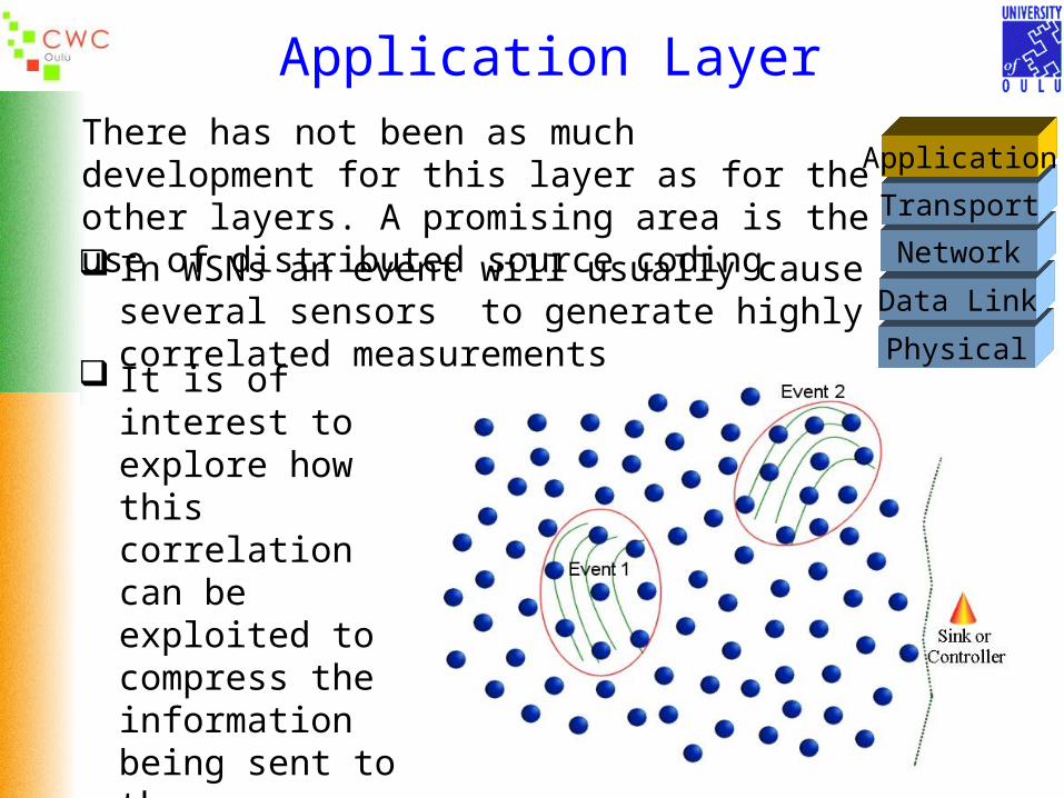
Application Layer
Physical
Data Link
Network
Transport
ApplicationThere has not been as much development for this layer as for the other layers. A promising area is the use of distributed source coding In WSNs an event will usually cause several sensors
to generate highly correlated measurements
It is of interest to explore how this correlation can be exploited to compress the information being sent to the controller or sink node

Distributed Source CodingExample Assume that the measurements X and Y are correlated Y is available at the decoder on the sink node but not at the node where X
is encoded How can X be encoded in a compressed manner knowing that Y is
available at the decoder?
NYX N is a random variable that represents the correlation between X and Y. If N is Gaussian, one can get the same performance by knowing only the statistics of N at the encoder as when Y is known at the encoder

Distributed Source Coding
Consider an 8-level scalar quantizer and the correlated variables X and Y Partition the set of 8 quantization levels into 2 cosets (even and odd levels) If Y is available at the decoder only the index of the coset containing X, the
red coset, is needed to be transmitted (1 bit) Knowing Y, the decoder finds the closest quantization level in the red
coset and estimates that X takes on the value r4
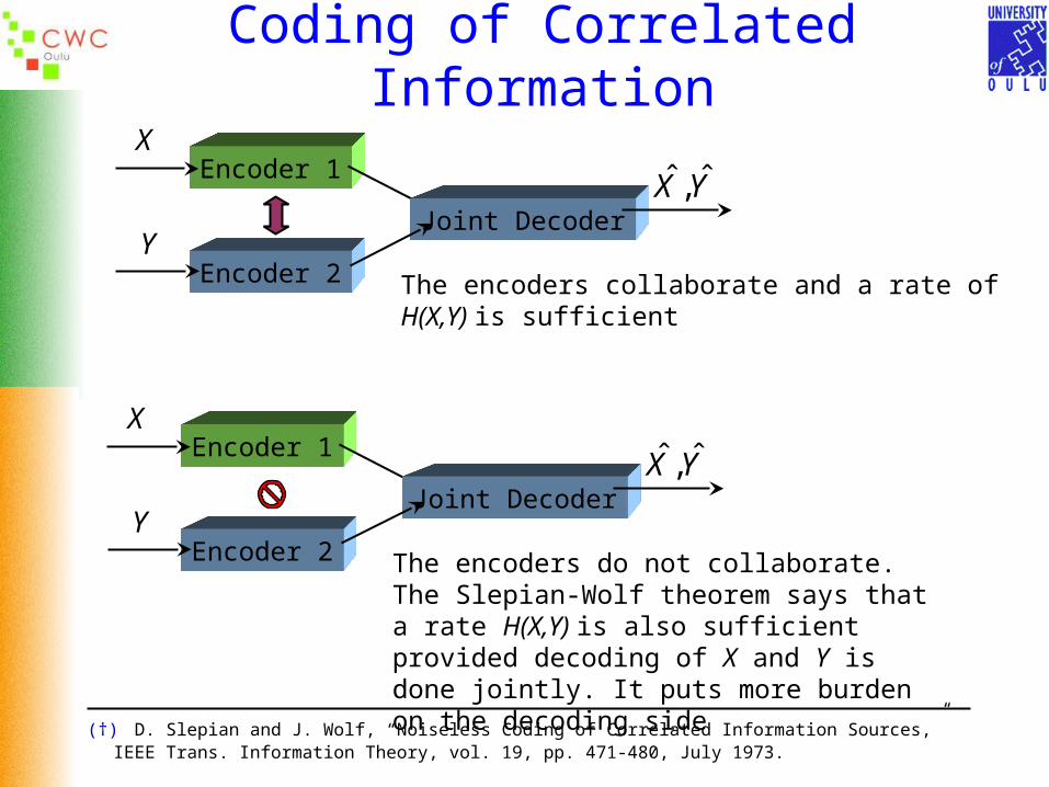
Coding of Correlated Information
(†) D. Slepian and J. Wolf, “Noiseless Coding of Correlated Information Sources,” IEEE Trans. Information Theory, vol. 19, pp. 471-480, July 1973.
The encoders collaborate and a rate of H(X,Y) is sufficient
Encoder 1
Encoder 2
Joint Decoder
X
Y
YX ˆ,ˆ
The encoders do not collaborate. The Slepian-Wolf theorem says that a rate H(X,Y) is also sufficient provided decoding of X and Y is done jointly. It puts more burden on the decoding side
Encoder 1
Encoder 2
Joint Decoder
X
Y
YX ˆ,ˆ
Some Final Words New Paradigm – WSNs do not have many of the features of the
conventional networks for which the OSI protocol layer stack model has proven to be successful. Therefore it is quite possible that a different mix of layers might prove to be more efficient for many WSN applications
Avoid Conflicting Behavior – For example a routing protocol that favors smaller hops to save transmission energy consumption does require a proper MAC protocol to coordinate the transmissions along the data flow to minimize contention and keep the transceivers off as much as possible
Remove Unnecessary Layers – Some applications do not require all layers
WSNs provide a rich source of problems in communication protocols, sensor tasking and control, sensor fusion, distributed data bases, and algorithmic design