ceos water constellation feasibility...
TRANSCRIPT

CEOSWater ConstellationFeasibility Study
Version 1.0October 2015
Version 1.0October 2016

1
October 23, 2016
CEOS Water Constellation Feasibility Study Report
Contributors to the Report This report was prepared by members of the Committee on Earth Observation Satellites (CEOS) Water Strategy Implementation Study Team (WSIST) and experts from the water community, many of whom are members of the GEO Integrated Global Water Cycle Observations (IGWCO) Community of Practice (CoP). Contributions include chapters, sections, paragraphs, useful suggestions, and review comments. CEOS Agencies Bojan Bojkov* ESA/EUMETSAT Marie-Josée Bourassa* CSA Selma Cherchali* CNES Arnold Dekker* CSIRO Bradley Doorn NASA George Dyke JAXA Jared Entin* NASA Ralph Ferraro* NOAA Kinji Furukawa JAXA Yukio Haruyama JAXA George Huffman NASA Chu Ishida* JAXA John W. Jones* USGS Misako Kachi JAXA Bob Kuligowski* NOAA Takashi Maeda JAXA Forrest Melton NASA Steve Neeck NASA Riko Oki JAXA Matthew Rodell NASA Jonathon Ross* Geoscience Australia (GA) Kerry Sawyer* NOAA Matthew Steventon JAXA Stephen Ward JAXA Shizu Yabe JAXA Moeka Yamaji JAXA Xiwu Zhan NOAA IGWCO and water experts Vanessa Aellen GEO Secretariat Stéphane Bélair ECCC/Canada

2
Dominique Berod WMO Andrée-Anne Boisvert U of Manitoba Wolfgang Grabs BAFG Toshio Koike U Tokyo Richard Lawford Morgan State University Ulrich Looser BAFG Heather McNairn AAFC/Canada Massimo Menenti U Delft, the Netherlands Bob Su ITC, the Netherlands *WSIST members Thanks also go to any people not listed above who provided comments and inputs to the Report and were inadvertently left off this listing.

3
Table of Contents 1. Introduction ............................................................................................................................ 5
1.1 Background .................................................................................................................... 5 1.2 Audience ......................................................................................................................... 5 1.3 Linkages with major international agreements .............................................................. 5 1.4 Purpose of the CEOS Water Constellation Feasibility Study ........................................ 7 1.5 Approach of the Feasibility Study .................................................................................. 8 1.6 Assessment of user needs ............................................................................................... 8
2. Relationships among priority water cycle variables .............................................................. 9 3. Existing and planned satellite observations for precipitation and soil moisture .................. 12
3.1 Precipitation .................................................................................................................... 12 a. Confirmation of the validated requirements .................................................................. 12 b. List of missions confirmed as contributing to the requirement ..................................... 14 c. Assess gaps between 2016 and 2021 ............................................................................. 19 d. Possible coordination of CEOS missions ...................................................................... 23 e. Benefits and economic considerations .......................................................................... 24
3.2 Soil moisture ................................................................................................................ 26 a. Confirmation of the validated requirements .................................................................. 26 b. List of missions confirmed as contributing to the requirement ..................................... 28 c. Assess gaps between 2016 and 2021 ............................................................................. 29 d. Possible coordination of CEOS missions ...................................................................... 31 e. Benefits and economic considerations .......................................................................... 31
3.3 Evapotranspiration ........................................................................................................ 33 a. Confirmation of validated requirements ........................................................................ 33 b. List of missions confirmed as contributing to the requirement ..................................... 35 c. Assess gaps between 2016 and 2021 ............................................................................. 36 d. Possible coordination of CEOS missions ...................................................................... 37 e. Benefits and economic considerations .......................................................................... 37
3.4 River discharge ............................................................................................................. 38 a. Confirmation of validated requirements ........................................................................ 39 b. List of missions confirmed as contributing to the requirement ..................................... 39 c. Assess gaps between 2016 and 2021 ............................................................................. 42 d. Possible coordination of CEOS missions ...................................................................... 43 e. Benefits and economic considerations .......................................................................... 43
3.5 Surface water storage ................................................................................................... 44

4
a. Confirmation of validated requirements ........................................................................ 44 b. List of missions confirmed as contributing to the requirement ..................................... 45 c. Assess gaps between 2016 and 2021 ............................................................................. 47 d. Possible coordination of CEOS missions ...................................................................... 48 e. Benefits and economic considerations .......................................................................... 48
3.6 Groundwater ................................................................................................................. 49 a. Confirmation of validated requirements ........................................................................ 49 b. Define a list of missions confirmed as contributing to the requirement ....................... 50 c. Assess gaps between 2016 and 2021 ............................................................................. 50 d. Possible coordination of CEOS missions ...................................................................... 51 e. Benefits and economic considerations .......................................................................... 52
4. Priority water cycle variable synergistic observation feasibility ......................................... 53 4.1 Define synergistic observation requirements for high-priority parameters .................. 53 4.2 Summary of the synthesis results ................................................................................. 58
5. Recommendations regarding the Water Constellations ....................................................... 63 6. Way forward ........................................................................................................................ 64 7. References ............................................................................................................................ 66 Appendix .................................................................................................................................. 68
A Relevant CEOS missions ................................................................................................ 68 B GCOS/ECV ..................................................................................................................... 68 C WMO/SOG ..................................................................................................................... 68 D List of Acronyms ............................................................................................................ 68

5
1. Introduction 1.1 Background This report was prepared by the Committee on Earth Observation Satellites’ (CEOS) Water Strategy Implementation Study Team (WSIST) to provide a response to the Group on Earth Observation System of Systems (GEOSS) Water Strategy. The Group on Earth Observations (GEO), which coordinates the development of the GEOSS Water Strategy, issued the Strategy at the GEO-Plenary X in January 2014 and requested that CEOS and other organizations provide observations and information services to respond to the Strategy’s recommendations related to observational systems. CEOS WSIST prepared its response to the Strategy’s recommendations (CEOS Water Strategy), which was approved by the 29th CEOS Plenary held in Kyoto on November 4-5, 2015. The Plenary decided to extend WSIST for one year in order to implement the actions proposed in the CEOS Water Strategy, including a feasibility study (FS) of the CEOS Virtual Water Constellation (GEOSS Water Strategy recommendation C.1):
“The feasibility of developing a Water-Train satellite constellation should be assessed. This suite of satellites would be modelled after the A-Train, providing a space segment of an observation system that would capture all fluxes and stores of the water cycle using a diverse suite of platforms and instruments. This system would operate as a Virtual Water Cycle Constellation.”
WSIST agreed to focus on six high-priority variables associated with the water cycle: precipitation, soil moisture, evaporation/evapotranspiration, river discharge, surface water storage, and ground water. WSIST carried out a gap analysis of individual observation systems for the parameters and their combined observation system. The goal of the FS is to address all six parameters and optimize the integrated observation system. Given the complexity of assessing the interactions between all six variables, WSIST proposed a step-wise approach at the SIT-30 meeting held in Frascati, Italy on April 18, 2016. Based on this proposal, members agreed that WSIST would start with the precipitation-soil moisture case study and then expand to other variables. 1.2 Audience The main audience for this report is CEOS and its member organizations, hereafter referred to as CEOS Agencies. The report will serve primarily as an internal document to highlight priorities, identify opportunities for improved coordination and synergy, and provide guidance in planning future water-related missions. Some of the ideas and discussions are expected to filter into documents, surveys, and other priority-setting exercises. Depending on the robustness of the results and the perceived value of the methodology used to achieve them, this experience may be documented in scientific literature. 1.3 Linkages with major international agreements The virtual satellite constellation for water cycle observations considered by this FS will

6
directly address the space component of the GEOSS Water Societal Benefit Area (SBA). It will also support the following major international agreements: Sendai Framework for Disaster Risk Reduction 2015-2030 (March 2015): The water cycle satellite constellation will help organizations understand disaster risks at national/local levels and regional/global levels by collecting, analysing, managing, and using relevant data and information. The Constellation would support access to multi-hazard early warning systems, particularly in the case of floods and drought. Transforming our world: The 2030 Agenda for Sustainable Development (September 2015): The water cycle satellite constellation will support Goal 6 of the Sustainable Development Goals: Clean water and sanitation, and its relevant targets and indicators. The UN High Level Panel on Water agreed on an action plan for the SDG 6 (Water and Sanitation), providing framework for implementing the related activities in September 2016. (see https://sustainabledevelopment.un.org/content/documents/11280HLPW_Action_Plan_DEF_11-1.pdf) Paris Agreement (December 2015): Article 7 (Adaptation) (c) calls for strengthening scientific knowledge on climate, including research, and systematic observation of climate and early warning systems in a manner that informs climate services and supports decision-making. The FS will directly address systematic observation of the climate system and early warning systems. Ramsar Convention: This intergovernmental treaty provides the framework for national action and international cooperation for the conservation and wise use of wetlands and their resources. The Convention includes all lakes and rivers, underground aquifers, swamps and marshes, wet grasslands, peatlands, oases, estuaries, deltas and tidal flats, mangroves and other coastal areas, coral reefs, and all human-made sites such as fish ponds, rice paddies, reservoirs, and salt pans. Their observation is necessary for understanding and managing these sites. In order to address high profile issues it is useful to identify which variables will contribute to the activities. They are identified Table 1.3.1 below. Table 1.3.1. Data needs for major agreements. Precipitation Soil
Moisture Evapo- transpiration
River Discharge
Water Storage
Ground Water
Sendai Framework for Disaster Risk and Development
*
*
**
*
Agenda for Sustainable Development
* * * * * *

7
Paris Agreement on Climate Change
*
*
*
*
Ramsar Convention on Biodiversity
*
*
*
**
*
1.4 Purpose of the CEOS Water Constellation Feasibility Study The FS aims to provide an assessment of the value and feasibility of a constellation that could measure water cycle components and synchronize them in time and space. The FS assesses options for providing this integrated capability. At present, the water cycle measurements are taken from different platforms with widely varying measurement techniques at different intervals, resolutions ,and sampling strategies, making their synergistic use very difficult. The FS will lead to an understanding of the connections among observing systems for individual variables in terms of requirements and capabilities and will form a framework that will enable new missions to be more effectively coordinated with existing and planned missions. In the longer term, the study could provide a basis for planning that anticipates where new satellite missions could make the greatest contribution to the study of the water cycle. For example, new agendas for climate change, sustainable development, biodiversity, and disaster risk reduction will all place new requirements on the existing and planned observational system. In some cases, measurements of an individual variable will be key to meeting international requirements and, in other cases, a mix of variables will be needed to monitor conditions. The overall effort could lead to more valuable measurements since they will be compared and integrated with measurements taken in the same time and space framework, thereby providing more accurate assessments of all aspects of the water cycle. This framework could also provide the basis for assessing economic benefits of adding a sensor on a planned mission versus the launch of a new platform dedicated to one or two water cycle variables. It may also help ensure that new missions are implemented in a way that allows maximum benefit for all water cycle variables. The links between applications and international conventions have already been introduced (See Section 1.2.). Primary applications of these integrated observations would include: improvements in flood prediction, warning, and monitoring; drought monitoring and prediction; assessment of water resource availability on all time scales; and environmental monitoring in remote areas where development is taking place but no measurements are available. Closing the water cycle is an essential research activity that supports all of these applications. Water cycle closure is expected to contribute to better hydrologic modelling, which will in turn provide better soil moisture, runoff, and aquifer recharge predictions and lead to new and more reliable operational services. Additionally, many of these parameters
8
could help improve weather and climate model initializations, leading to more accurate predictions. 1.5 Approach of the Feasibility Study The FS features a gap analysis between current and future observation systems based on the priority variables that were documented as Essential Water Variables (EWVs) in the GEOSS Water Strategy and most of which will be recognized as Essential Climate Variables (ECVs) by GCOS as of 2016. (The only exception is evapotranspiration, the inclusion of which is high desirable and will be discussed in the ongoing review of GCOS Implementation Plan.) Gaps were identified by comparing their observation requirements and current and planned observation capabilities. Countermeasures are proposed to fill identified gaps. In addition to single-variable gap analysis, the FS considers the combined capabilities of those parameter observation systems. After the gap analysis, analysis and discussion focuses on identifying actions to fill the gaps between the combined requirements and capabilities, with optimization of the entire integrated observation system to cover the six variables identified as high priority. Recognizing the difficulty of trying to address interactions among all the variables, WSIST began its analysis with a case study of precipitation and soil moisture observation systems and their potential to be integrated into a more synergistic observation system. Observation requirements for precipitation and soil moisture are based on existing statements of requirements and then compared with relevant existing and planned CEOS satellite mission capabilities. The report makes specific recommendations for CEOS to address gaps. For the gap analysis, CEOS Principals noted the importance of a sampling study; it has been given due consideration in this report. Based on the success of this approach, the technique was applied to the other four variables. 1.6 Assessment of user needs A very critical part of this effort is to determine what users actually require in terms of measurements to identify where needs can be met by combining data products, datasets, and even aspects of observational systems. Addressing the needs identified by the GEOSS Water Strategy is very important. In addition, a thorough review was recently undertaken as part of GEO Task US-09-01a: Critical Earth Observations Priorities-Water Societal Benefit Area, US-09-01a (Task Lead: Lawrence Friedl, USA/NASA; Water SBA Analyst: Sushel Unninayar, UMBC, 2010; hereafter referred as “GEO Water SBA requirements”). The review articulates the critical Earth observation priorities for the Water SBA. The report addresses four sub-areas associated with terrestrial hydrology and water resources: surface waters, underground waters, forcing on terrestrial hydrological elements, and water quality/use. The study addresses the “demand” side of observation needs and priorities. More than 200 papers and reports were analysed by experts, who also considered global, regional and local aspects of observational requirements. They also assessed requirements for derived information products relevant to the management of terrestrial water resources and the terrestrial water cycle. In addition to the GEO Water SBA requirements, GCOS ECV requirements and WMO-SOG requirements were reviewed in the study.

9
2. Relationships among priority water cycle variables Climate change has a significant impact on regional river discharge and water availability, which is most important for water resource managers and policy-makers. By 2050, drought-affected areas will likely increase in some water-stressed regions, while flood risks are likely to increase in some wet areas. Under this circumstance, it is critical to integrate the knowledge of the atmosphere and hydrology communities for improved prediction capability related to available water resources and possible hazards (floods and droughts). In order to develop an integrated understanding and monitoring capability, we need a better way of representing the actual conditions at any point in time. This can come through observational systems, or data assimilation, or some combination of both. Developing an integrated observing system calls for an understanding of the relationships and potential synergies between the measurements of different variables. The second approach, which has seen major advances over the past two decades, uses models and data assimilation systems to integrate information, especially where observational systems are inadequate or too rigid to adjust to new demands. Assimilation systems can be used to interpolate data, generate estimates of variables that are currently not measured (e.g., root zone soil moisture), and produce spatially uniform fields that facilitate large-scale analysis. Furthermore, prediction systems rely on assimilation systems for their initial conditions; hence, advances in this area will lead to improvements in predictive capability. Distributed hydrological models (DHMs) can provide explicit distributed representation of the spatial variation and physical descriptions of runoff generation and routing in river channels from basin to continental scales. Land surface models (LSMs) express credible representations of water and energy fluxes in the soil-vegetation-atmosphere transfer system. The coupling of LSMs and DHMs has improved land surface representation, benefiting the streamflow prediction capabilities of hydrological models and providing improved estimates of water and energy fluxes into the atmosphere. Introducing a dynamic vegetation model (DVM) into the LSM-DHM coupled model develops an eco-hydrological model to calculate river discharge, groundwater, energy flux, and vegetation dynamics as diagnostic variables at the basin scale within a distributed hydrological modelling framework. Land data assimilation systems (LDAS) consisting of a LSM as the model operator, a radiative transfer model (RTM) at microwave frequencies as the observation operator, and a choice of assimilation schemes can considerably improve soil moisture and surface fluxes. By using a LSM coupled with a DVM as the observation operator, a new LDAS has been developed for simultaneously simulating surface soil moisture, root-zone soil moisture, and vegetation dynamics. It assimilates passive microwave observations that are sensitive to both surface soil moisture and terrestrial biomass. Coupling an LDAS and a mesoscale atmospheric model can introduce the effects of land surface conditions on the atmospheric circulation. Furthermore, a coupled land and atmosphere data assimilation system (CALDAS) can overcome the drifts owing to predicted model forcing (i.e., solar radiation and rainfall) and then improve representation of cloud distribution and associated rainfall events.

10
A water cycle constellation, especially for rainfall and soil moisture, can integrate satellite observation data into these sophisticated hydrological models and assimilation systems to improve flood and drought prediction capability, contribute to water-related disaster risk reduction, and strengthen water resources management. Figure 2.1 illustrates the major components of the water cycle (and their ties to the energy cycle) and how satellite missions provide data for many (but not all) of the components. Note that not all of these missions provide data at the desired resolution and accuracy. Assimilation and modelling are key to filling in the missing parts, as illustrated in Figure 2.2.
Figure 2.1. Illustration of how satellite missions provide observations of the water cycle, as well as instruments addressing the energy cycle. (after Cherchali and Gosset, 2016)

11
Figure 2.2. Water cycle variables and their relationships (Courtesy: Toshio Koike)
12
3. Existing and planned satellite observations for precipitation and soil moisture 3.1 Precipitation Precipitation is liquid or solid water that falls to the surface from the atmosphere. It is associated with a wide variety of coherent atmospheric phenomena, from small convective showers to continental-scale monsoons. Organized precipitating systems have precipitation rates ranging from less than 1 mm/hour to more than 100 mm/hour, spatial scales from less than 1 km to more than 1000 km, and temporal scales of minutes to seasons. Their modes of variability include diurnal, synoptic, intraseasonal, seasonal, annual, inter-annual, or longer. Precipitation has a very direct and significant influence on the quality of human life in terms of meeting critical needs, such as water for drinking and agriculture. Timely, high-quality precipitation observations, with global, long-term coverage and frequent sampling, are crucial to understanding and predicting the Earth’s climate, weather, global water, and energy cycle processes and their consequences for life on Earth. Improved observations of precipitation, their reporting, and their timely distribution are central to meeting the needs outlined in Section 3.1 a (below). Research has shown that a lack of adequate observational data limits the ability to quantify precipitation inputs and, consequently, limits the ability to close water budgets. The amount, rate, and type of precipitation largely determine our freshwater supply. The physical characteristics of liquid and solid water in the atmosphere, including droplet and ice size, shape, and temperature, are crucial to determining the nature of precipitation. Ideally, precipitation observations should provide not only the actual amount reaching the ground, but also the associated vertical hydrometeor structure. Latent heating, which results from the condensation of water vapour into clouds and precipitation, is an important forcing function for large-scale atmospheric circulation, thus establishing a key link to the global energy cycle. Precipitation falling into the ocean affects ocean salinity and significantly impacts atmosphere-ocean interactions on inter-annual time scales. Over land, the frequency and intensity of precipitation strongly influences critical aspects of surface hydrology, including runoff, soil moisture, and streamflow. Extremes in precipitation occurrence and intensity, which drive floods and droughts, have an enormous impact on human society, agriculture, and the natural environment. a. Confirmation of the validated requirements GEO Water SBA requirements for precipitation are provided in Table 3.1.1. The wide range of requirements, varying by use, is apparent. It should be noted that these are requirements for aggregated data products. All specifications are application(s)-dependent, particularly latency. The upper limit to accuracy specifications typically refers to the “desired” figure, not operational availability.
13
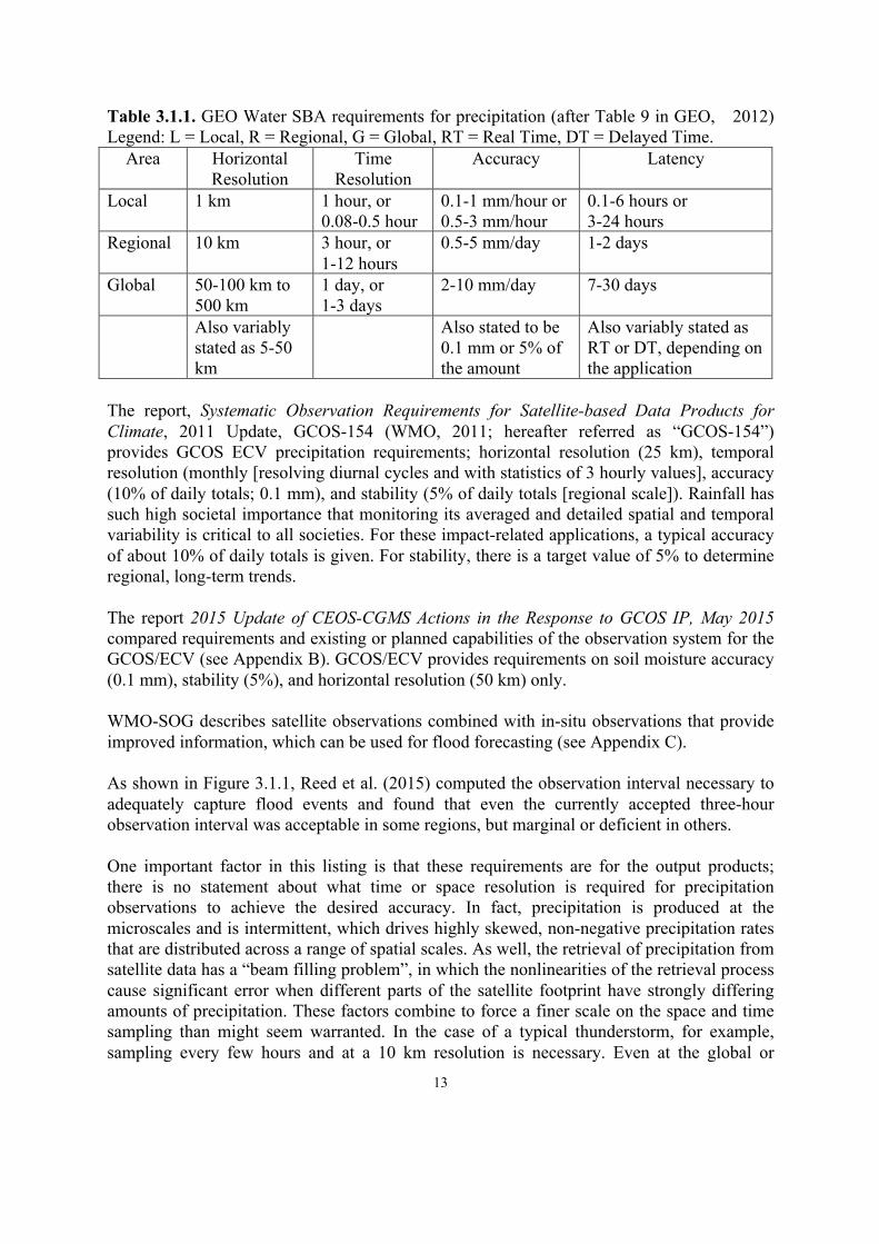
Table 3.1.1. GEO Water SBA requirements for precipitation (after Table 9 in GEO, 2012) Legend: L = Local, R = Regional, G = Global, RT = Real Time, DT = Delayed Time.
Area Horizontal Resolution
Time Resolution
Accuracy Latency
Local 1 km
1 hour, or 0.08-0.5 hour
0.1-1 mm/hour or 0.5-3 mm/hour
0.1-6 hours or 3-24 hours
Regional 10 km
3 hour, or 1-12 hours
0.5-5 mm/day 1-2 days
Global 50-100 km to 500 km
1 day, or 1-3 days
2-10 mm/day 7-30 days
Also variably stated as 5-50 km
Also stated to be 0.1 mm or 5% of the amount
Also variably stated as RT or DT, depending on the application
The report, Systematic Observation Requirements for Satellite-based Data Products for Climate, 2011 Update, GCOS-154 (WMO, 2011; hereafter referred as “GCOS-154”) provides GCOS ECV precipitation requirements; horizontal resolution (25 km), temporal resolution (monthly [resolving diurnal cycles and with statistics of 3 hourly values], accuracy (10% of daily totals; 0.1 mm), and stability (5% of daily totals [regional scale]). Rainfall has such high societal importance that monitoring its averaged and detailed spatial and temporal variability is critical to all societies. For these impact-related applications, a typical accuracy of about 10% of daily totals is given. For stability, there is a target value of 5% to determine regional, long-term trends. The report 2015 Update of CEOS-CGMS Actions in the Response to GCOS IP, May 2015 compared requirements and existing or planned capabilities of the observation system for the GCOS/ECV (see Appendix B). GCOS/ECV provides requirements on soil moisture accuracy (0.1 mm), stability (5%), and horizontal resolution (50 km) only. WMO-SOG describes satellite observations combined with in-situ observations that provide improved information, which can be used for flood forecasting (see Appendix C). As shown in Figure 3.1.1, Reed et al. (2015) computed the observation interval necessary to adequately capture flood events and found that even the currently accepted three-hour observation interval was acceptable in some regions, but marginal or deficient in others. One important factor in this listing is that these requirements are for the output products; there is no statement about what time or space resolution is required for precipitation observations to achieve the desired accuracy. In fact, precipitation is produced at the microscales and is intermittent, which drives highly skewed, non-negative precipitation rates that are distributed across a range of spatial scales. As well, the retrieval of precipitation from satellite data has a “beam filling problem”, in which the nonlinearities of the retrieval process cause significant error when different parts of the satellite footprint have strongly differing amounts of precipitation. These factors combine to force a finer scale on the space and time sampling than might seem warranted. In the case of a typical thunderstorm, for example, sampling every few hours and at a 10 km resolution is necessary. Even at the global or

14
climate scale, it is becoming standard to discuss the climatology of “extremes”. In this case, one is essentially forced back to the few-hour, 10-km sampling to capture the highly focused space and time events that constitute extremes. Figure 3.1.1. Hydrological model-based estimate of the temporal resolution of satellite-based precipitation observations (in hours) required to maintain acceptable flood predictions. Grayed-out areas denote locations where either the hydrologic model lacked acceptable performance relative to historical streamflow observations or historical data was insufficient to make an assessment. (Reed et al., 2015) b. List of missions confirmed as contributing to the requirement Existing and planned mission capabilities are listed in Appendix A, Tables A.1.1 and A.1.2. GPM constellation satellites consist of the GPM core satellite carrying DPR and GMI and international partners’ satellites carrying microwave imagers (MWIs) and microwave sounders (MWSs). It is a challenge to maintain this constellation and its datasets. When the GPM core satellite was launched in February 2014, the initial GPM-era constellation consisted of microwave conical-scan “imagers” (DMSP F15 SSMI [limited]; DMSP F16, F17, and F18 SSMIS; GCOM-W1 AMSR2; GPM GMI) and microwave cross-track-scan “sounders” (NOAA-18, NOAA-19, Metop-A, and Metop-B MHS; Megha-Tropiques SAPHIR; SNPP ATMS), referred hereafter to as MWI and MWS. NASA and JAXA are studying the post-GPM mission and hold regular technical meetings for information exchange.

15
At the time of this writing, some two-and-a half years later, the DMSP F-19 satellite failed recently on orbit and F-20 is in storage but it will likely not be launched. F-18, F-17, and F-16 are in service beyond their designed lifetimes. F-15 is not functioning properly. The impending loss of DMSP microwave radiometers in early-morning orbit will significantly reduce sampling of the diurnal water cycle, making it necessary to rely more heavily on sounders for precipitation remote sensing. Such a shift in data source will degrade the overall quality of the precipitation dataset since sounders are not optimally designed for precipitation rate retrieval due to their variable footprint size (in contrast with the fixed footprint size of conical scanners), their channel selection (focused more on absorption bands for sounding than on window bands which are more suited for precipitation remote sensing), and the lack of polarization information (which provides additional information since precipitation tends to depolarize the signal from the lower atmosphere).. In addition, the lower sampling rate will degrade the Constellation’s ability to provide the three-hourly observation interval at all times of day, which is considered the minimum to effectively monitor most precipitation events (see, for example, Wood et al., 2015). GCOM-W was originally planned as a three-generation satellite program. The first GCOM-W satellite was launched in 2012. Recognizing the significant role of AMSR-2 and its predecessor, Aqua/AMSR-E, for climate research and operational services in the world, the Japanese government decided to accelerate its study of the GCOM-W follow-on mission in 2016. The AMSR-2 follow-on mission will be a very similar MWI mission and it may be improved by the addition of 183 GHz channel (currently under consideration). The type of satellite sensor is very important. For example, a standard MWS scans perpendicular to the satellite track, creating a continuously varying Earth incidence angle that causes footprints at each angle away from the nadir to take a different size and shape, precluding the use of polarization information. The MWI is strongly preferred. The Chinese Academy of Science is studying the Water Cycle Observation Mission (WCOM). (see http://eo-water.radi.ac.cn/en/highlight_detail.php?id=1). Various global precipitation maps are produced by combining several satellite datasets with surface gauge data (see Table 3.1.2) and by combining input data from several satellite sensor types (see Table 3.1.3). The combination of geostationary and LEO satellites and in-situ data allow the geospatial consistency of satellite data to be combined with high-frequency in-situ observations. Infrared data from geostationary satellites that supplement microwave precipitation information (and enables meeting the rapid refresh and short latency requirements) are provided by NOAA (currently GOES-13 over the Pacific Ocean and western Americas and GOES-15 over the Atlantic Ocean and eastern Americas), EUMETSAT (currently METEOSAT-10 over Europe and Africa and METEOSAT-7 over Central Asia), and JAXA (Himawari-8 over East Asia and the Western Pacific). These capabilities will be maintained in the long term and will even be enhanced: the next-generation GOES, with significantly improved spatial, temporal, and spectral coverage will launch in late 2016. EUMETSAT will deploy Meteosat Third Generation (MTG) beginning in 2020 and will replace METEOSAT-7 with the more advanced METEOSAT-8 in early 2017. Other nations’ geostationary satellites
16
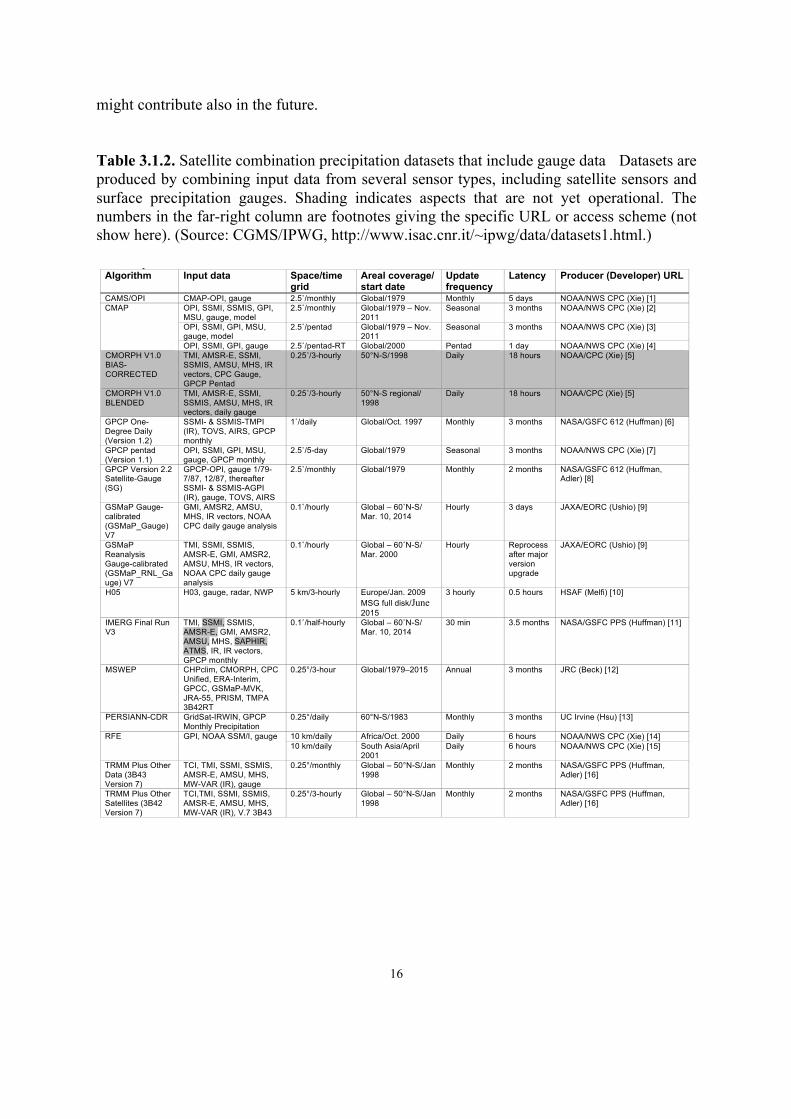
might contribute also in the future. Table 3.1.2. Satellite combination precipitation datasets that include gauge data Datasets are produced by combining input data from several sensor types, including satellite sensors and surface precipitation gauges. Shading indicates aspects that are not yet operational. The numbers in the far-right column are footnotes giving the specific URL or access scheme (not show here). (Source: CGMS/IPWG, http://www.isac.cnr.it/~ipwg/data/datasets1.html.)
Combination Data Sets with Gauge Data Table 1. Summary of publicly available, quasi-operational, quasi-global precipitation estimates that are produced by combining input data from several sensor types, including satellite sensors and precipitation gauges. Where appropriate, the algorithms applied to the individual input data sets are mentioned. Solid shading indicates products that are not yet available. [Last updated 21 June 2016, G.J. Huffman] Algorithm Input data Space/time
grid Areal coverage/ start date
Update frequency
Latency Producer (Developer) URL
CAMS/OPI CMAP-OPI, gauge 2.5˚/monthly Global/1979 Monthly 5 days NOAA/NWS CPC (Xie) [1] CMAP OPI, SSMI, SSMIS, GPI,
MSU, gauge, model 2.5˚/monthly Global/1979 – Nov.
2011 Seasonal 3 months NOAA/NWS CPC (Xie) [2]
OPI, SSMI, GPI, MSU, gauge, model
2.5˚/pentad Global/1979 – Nov. 2011
Seasonal 3 months NOAA/NWS CPC (Xie) [3]
OPI, SSMI, GPI, gauge 2.5˚/pentad-RT Global/2000 Pentad 1 day NOAA/NWS CPC (Xie) [4] CMORPH V1.0 BIAS-CORRECTED
TMI, AMSR-E, SSMI, SSMIS, AMSU, MHS, IR vectors, CPC Gauge, GPCP Pentad
0.25˚/3-hourly 50°N-S/1998 Daily 18 hours NOAA/CPC (Xie) [5]
CMORPH V1.0 BLENDED
TMI, AMSR-E, SSMI, SSMIS, AMSU, MHS, IR vectors, daily gauge
0.25˚/3-hourly 50°N-S regional/ 1998
Daily 18 hours NOAA/CPC (Xie) [5]
GPCP One-Degree Daily (Version 1.2)
SSMI- & SSMIS-TMPI (IR), TOVS, AIRS, GPCP monthly
1˚/daily Global/Oct. 1997 Monthly 3 months NASA/GSFC 612 (Huffman) [6]
GPCP pentad (Version 1.1)
OPI, SSMI, GPI, MSU, gauge, GPCP monthly
2.5˚/5-day Global/1979 Seasonal 3 months NOAA/NWS CPC (Xie) [7]
GPCP Version 2.2 Satellite-Gauge (SG)
GPCP-OPI, gauge 1/79-7/87, 12/87, thereafter SSMI- & SSMIS-AGPI (IR), gauge, TOVS, AIRS
2.5˚/monthly Global/1979 Monthly 2 months NASA/GSFC 612 (Huffman, Adler) [8]
GSMaP Gauge-calibrated (GSMaP_Gauge) V7
GMI, AMSR2, AMSU, MHS, IR vectors, NOAA CPC daily gauge analysis
0.1˚/hourly Global – 60˚N-S/ Mar. 10, 2014
Hourly 3 days JAXA/EORC (Ushio) [9]
GSMaP Reanalysis Gauge-calibrated (GSMaP_RNL_Gauge) V7
TMI, SSMI, SSMIS, AMSR-E, GMI, AMSR2, AMSU, MHS, IR vectors, NOAA CPC daily gauge analysis
0.1˚/hourly Global – 60˚N-S/ Mar. 2000
Hourly Reprocess after major version upgrade
JAXA/EORC (Ushio) [9]
H05 H03, gauge, radar, NWP 5 km/3-hourly Europe/Jan. 2009 MSG full disk/June 2015
3 hourly 0.5 hours HSAF (Melfi) [10]
IMERG Final Run V3
TMI, SSMI, SSMIS, AMSR-E, GMI, AMSR2, AMSU, MHS, SAPHIR, ATMS, IR, IR vectors, GPCP monthly
0.1˚/half-hourly Global – 60˚N-S/ Mar. 10, 2014
30 min 3.5 months NASA/GSFC PPS (Huffman) [11]
MSWEP CHPclim, CMORPH, CPC Unified, ERA-Interim, GPCC, GSMaP-MVK, JRA-55, PRISM, TMPA 3B42RT
0.25°/3-hour Global/1979–2015 Annual 3 months JRC (Beck) [12]
PERSIANN-CDR GridSat-IRWIN, GPCP Monthly Precipitation
0.25°/daily 60°N-S/1983 Monthly 3 months UC Irvine (Hsu) [13]
RFE GPI, NOAA SSM/I, gauge 10 km/daily Africa/Oct. 2000 Daily 6 hours NOAA/NWS CPC (Xie) [14] 10 km/daily South Asia/April
2001 Daily 6 hours NOAA/NWS CPC (Xie) [15]
TRMM Plus Other Data (3B43 Version 7)
TCI, TMI, SSMI, SSMIS, AMSR-E, AMSU, MHS, MW-VAR (IR), gauge
0.25°/monthly Global – 50°N-S/Jan 1998
Monthly 2 months NASA/GSFC PPS (Huffman, Adler) [16]
TRMM Plus Other Satellites (3B42 Version 7)
TCI,TMI, SSMI, SSMIS, AMSR-E, AMSU, MHS, MW-VAR (IR), V.7 3B43
0.25°/3-hourly Global – 50°N-S/Jan 1998
Monthly 2 months NASA/GSFC PPS (Huffman, Adler) [16]
[1] ftp://ftp.cpc.ncep.noaa.gov/precip/data-req/cams_opi_v0208/ [2] ftp://ftp.cpc.ncep.noaa.gov/precip/cmap/monthly/ [3] ftp://ftp.cpc.ncep.noaa.gov/precip/cmap/pentad/ [4] ftp://ftp.cpc.ncep.noaa.gov/precip/cmap/pentad_rt/ [5] ftp://ftp.cpc.ncep.noaa.gov/precip/CMORPH_V1.0 [6] ftp://rsd.gsfc.nasa.gov/pub/1dd-v1.2/ [7] ftp://ftp.cpc.ncep.noaa.gov/precip/GPCP_PEN/ [8] ftp://precip.gsfc.nasa.gov/pub/gpcp-v2.2/psg/ [9] http://sharaku.eorc.jaxa.jp/GSMaP/ [10] http://hsaf.meteoam.it/user-registration.php [11] ftp://arthurhou.pps.eosdis.nasa.gov/gpmdata/YYYY/MM/DD/imerg/ where YYYY, MM, DD are 4-digit year, 2-digit month, 2-digit day; automatic and free
registration required the first time [12] www.gloh2o.org [13] https://www.ncdc.noaa.gov/cdr/atmospheric/precipitation-persiann-cdr [14] ftp://ftp.cpc.ncep.noaa.gov/fews/newalgo_est/ [15] ftp://ftp.cpc.ncep.noaa.gov/fews/S.Asia/ [16] http://mirador.gsfc.nasa.gov/cgi-bin/mirador/presentNavigation.pl?tree=project&project=TRMM&dataGroup=Gridded

17
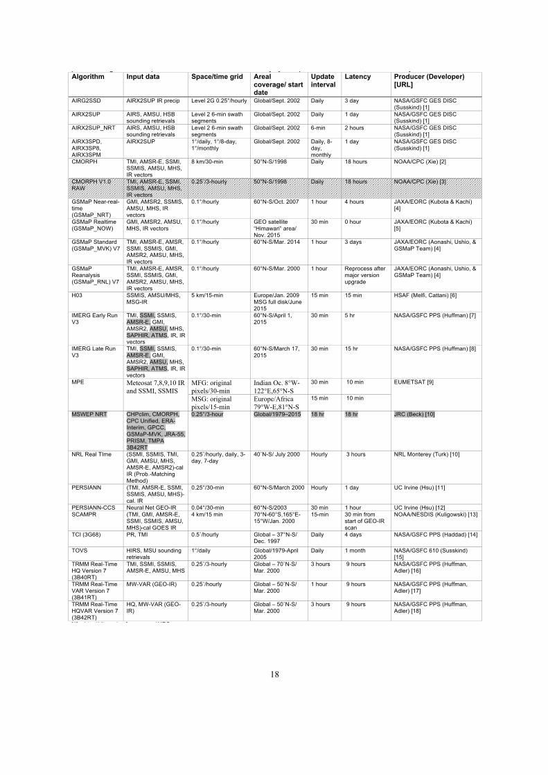
Table 3.1.3. Satellite combination precipitation datasets are produced by combining input data from several satellite sensor types. Shading indicates aspects that are not yet operational. Hatched shading indicates a product being released in phases. The numbers in the far-right column are footnotes giving the specific URL or access scheme (not show here). Source: CGMS/IPWG (http://www.isac.cnr.it/~ipwg/data/datasets2.html).
18
Satellite Combination Data Sets Table 2. Summary of publicly available, quasi-operational, quasi-global precipitation estimates that are produced by combining input data from several satellite sensor types. Where appropriate, the algorithms applied to the individual input data sets are mentioned. The TCI is available as a separate product from the Goddard DISC, in addition to the 3G68 compilation. Hatched shading indicates a product being released in phases – see site for current availability. [Last updated 21 June 2016, G.J. Huffman] Algorithm Input data Space/time grid Areal
coverage/ start date
Update interval
Latency Producer (Developer) [URL]
AIRG2SSD AIRX2SUP IR precip Level 2G 0.25°/hourly Global/Sept. 2002 Daily 3 day NASA/GSFC GES DISC (Susskind) [1]
AIRX2SUP AIRS, AMSU, HSB sounding retrievals
Level 2 6-min swath segments
Global/Sept. 2002 Daily 1 day NASA/GSFC GES DISC (Susskind) [1]
AIRX2SUP_NRT AIRS, AMSU, HSB sounding retrievals
Level 2 6-min swath segments
Global/Sept. 2002 6-min 2 hours NASA/GSFC GES DISC (Susskind) [1]
AIRX3SPD, AIRX3SP8, AIRX3SPM
AIRX2SUP 1°/daily, 1°/8-day, 1°/monthly
Global/Sept. 2002 Daily, 8-day, monthly
1 day NASA/GSFC GES DISC (Susskind) [1]
CMORPH TMI, AMSR-E, SSMI, SSMIS, AMSU, MHS, IR vectors
8 km/30-min 50°N-S/1998 Daily 18 hours NOAA/CPC (Xie) [2]
CMORPH V1.0 RAW
TMI, AMSR-E, SSMI, SSMIS, AMSU, MHS, IR vectors
0.25˚/3-hourly 50°N-S/1998 Daily 18 hours NOAA/CPC (Xie) [3]
GSMaP Near-real-time (GSMaP_NRT)
GMI, AMSR2, SSMIS, AMSU, MHS, IR vectors
0.1°/hourly 60°N-S/Oct. 2007 1 hour 4 hours JAXA/EORC (Kubota & Kachi) [4]
GSMaP Realtime (GSMaP_NOW)
GMI, AMSR2, AMSU, MHS, IR vectors
0.1°/hourly GEO satellite “Himawari” area/ Nov. 2015
30 min 0 hour JAXA/EORC (Kubota & Kachi) [5]
GSMaP Standard (GSMaP_MVK) V7
TMI, AMSR-E, AMSR, SSMI, SSMIS, GMI, AMSR2, AMSU, MHS, IR vectors
0.1°/hourly 60°N-S/Mar. 2014 1 hour 3 days JAXA/EORC (Aonashi, Ushio, & GSMaP Team) [4]
GSMaP Reanalysis (GSMaP_RNL) V7
TMI, AMSR-E, AMSR, SSMI, SSMIS, GMI, AMSR2, AMSU, MHS, IR vectors
0.1°/hourly 60°N-S/Mar. 2000 1 hour Reprocess after major version upgrade
JAXA/EORC (Aonashi, Ushio, & GSMaP Team) [4]
H03 SSMIS, AMSU/MHS, MSG-IR
5 km/15-min
Europe/Jan. 2009 MSG full disk/June 2015
15 min 15 min HSAF (Melfi, Cattani) [6]
IMERG Early Run V3
TMI, SSMI, SSMIS, AMSR-E, GMI, AMSR2, AMSU, MHS, SAPHIR, ATMS, IR, IR vectors
0.1°/30-min 60°N-S/April 1, 2015
30 min 5 hr NASA/GSFC PPS (Huffman) [7]
IMERG Late Run V3
TMI, SSMI, SSMIS, AMSR-E, GMI, AMSR2, AMSU, MHS, SAPHIR, ATMS, IR, IR vectors
0.1°/30-min 60°N-S/March 17, 2015
30 min 15 hr NASA/GSFC PPS (Huffman) [8]
MPE Meteosat 7,8,9,10 IR and SSMI, SSMIS
MFG: original pixels/30-min
Indian Oc. 8°W-122°E,65°N-S
30 min 10 min EUMETSAT [9]
MSG: original pixels/15-min
Europe/Africa 79°W-E,81°N-S
15 min 10 min
MSWEP NRT CHPclim, CMORPH, CPC Unified, ERA-Interim, GPCC, GSMaP-MVK, JRA-55, PRISM, TMPA 3B42RT
0.25°/3-hour Global/1979–2015 18 hr 18 hr JRC (Beck) [10]
NRL Real TIme (SSMI, SSMIS, TMI, GMI, AMSU, MHS, AMSR-E, AMSR2)-cal IR (Prob.-Matching Method)
0.25˚/hourly, daily, 3-day, 7-day
40˚N-S/ July 2000 Hourly 3 hours NRL Monterey (Turk) [10]
PERSIANN (TMI, AMSR-E, SSMI, SSMIS, AMSU, MHS)-cal. IR
0.25°/30-min 60°N-S/March 2000 Hourly 1 day UC Irvine (Hsu) [11]
PERSIANN-CCS Neural Net GEO-IR 0.04°/30-min 60°N-S/2003 30 min 1 hour UC Irvine (Hsu) [12] SCAMPR (TMI, GMI, AMSR-E,
SSMI, SSMIS, AMSU, MHS)-cal GOES IR
4 km/15 min 70°N-60°S,165°E-15°W/Jan. 2000
15-min 30 min from start of GEO-IR scan
NOAA/NESDIS (Kuligowski) [13]
TCI (3G68) PR, TMI 0.5˚/hourly
Global – 37°N-S/ Dec. 1997
Daily 4 days NASA/GSFC PPS (Haddad) [14]
TOVS HIRS, MSU sounding retrievals
1°/daily Global/1979-April 2005
Daily 1 month NASA/GSFC 610 (Susskind) [15]
TRMM Real-Time HQ Version 7 (3B40RT)
TMI, SSMI, SSMIS, AMSR-E, AMSU, MHS
0.25˚/3-hourly Global – 70˚N-S/ Mar. 2000
3 hours 9 hours NASA/GSFC PPS (Huffman, Adler) [16]
TRMM Real-Time VAR Version 7 (3B41RT)
MW-VAR (GEO-IR) 0.25˚/hourly Global – 50˚N-S/ Mar. 2000
1 hour 9 hours NASA/GSFC PPS (Huffman, Adler) [17]
TRMM Real-Time HQVAR Version 7 (3B42RT)
HQ, MW-VAR (GEO-IR)
0.25˚/3-hourly Global – 50˚N-S/ Mar. 2000
3 hours 9 hours NASA/GSFC PPS (Huffman, Adler) [18]
[1] http://disc.sci.gsfc.nasa.gov/AIRS [2] http://www.cpc.ncep.noaa.gov/products/janowiak/cmorph_description.html [3] ftp.cpc.ncep.noaa.gov/precip/CMORPH_V1.0 [4] http://sharaku.eorc.jaxa.jp/GSMaP/ [5] http://sharaku.eorc.jaxa.jp/GSMaP_NOW/ [6] http://hsaf.meteoam.it/user-registration.php [7] ftp://jsimpson.pps.eosdis.nasa.gov/data/imerg/early/; automatic and free registration required the first time [8] ftp://jsimpson.pps.eosdis.nasa.gov/data/imerg/late/; automatic and free registration required the first time [9] http://www.eumetsat.int/Home/Main/DataProducts/Atmosphere/index.htm?l=en [10] www.gloh2o.org

19
c. Assess gaps between 2016 and 2021 Figures 3.1.2 and 3.1.3 provide the timeline for known precipitation missions. The GPM core satellite is at a 65 degree inclined orbit, a non-sun-synchronous orbit that provides observations around the diurnal cycle every 83 days. The CEOS Precipitation Virtual Constellation (P-VC) is studying possible post-GPM missions. In 2016, three-hour global coverage requirements were marginally met at all times of day with the existence of the DMSP early orbit. However, in 2021, the likely disappearance of DMSP satellites will create a large gap in MWI observation options for 5 AM to 9 AM and 5 PM to 9 PM. This gap will be partially covered by MWS instruments, but IR data from GEO satellites will have to be used more often. This fall-back position of using less accurate data will degrade precipitation fields and affect other variables derived from precipitation.

20
Figure 3.1.2. Precipitation mission timeline.
LST 2016 2017 2018 2019 2020 2021 2022 2023 2024 2025 2026 2027012345678
9
10
1112
13
14
1516
17
1819
20
21
222324
DMSP F-16
DMSP F-17DMSP F-18
GCOM-W
FY-3AFY-3B
FY-3C
FY-3D
METEOR-M-N2
GPM-core
METOP-AMETOP-B
METOP-C
NPP
NOAA-18NOAA-19
MWIMWAS
Planned Extended
METOP-SG-b
JPSS-1
JPSS-2
FY-3E
FY-3F
FY-3G

21
Figure 3.1.3. Geostationary TIR mission timeline. Figure 3.1.4 provides the results of a precipitation observation sampling analysis in 2016 and 2021 (Yamaji, 2016). Considerable degradation of MWI sampling (the preferred instrument) from 2016 to 2021 is apparent. By including MWS (which is not optimal for retrieving precipitation), sampling interval will be improved. One additional consideration is that observing and quantifying light rain and falling snow using satellite observations is still a matter of research. These forms of precipitation often challenge the limits of detectability channel selection, even on the best, most current instruments. Nonetheless, these are the most common forms of precipitation at high latitudes and they have strong societal benefit implications for snowpack (and therefore hydrological analysis and water resources) and transport, among others. Current algorithm work focuses on the finest available resolution for frequencies above 100 GHz and the next generation of sensors must provide similar capabilities to provide useful input.
Longitude 2016 2017 2018 2019 2020 2021 2022 2023 2024 2025 2026 20270
137° / 75 ° W
0°-10 ° E
14.5°W-166 ° E
43.5°E/ 57.5° E
74° / 82° E
85.5° / 105° E
128.2° E
141° E
GOES-13
Operational Standby
GOES-14GOES-15
GOES-R GOES-S
GOES-TMETEOSAT-9METEOSAT-10
METEOSAT-11 MTG-I1
MTG-I2Electro-LN2Electro-LN3
Electro-LN4Electro-MN1
Electro-MN2
METEOSAT-7METEOSAT-8
Kalpana-1INSAT-3D
INSAT-3DR INSAT-3DS
FY-2EFY-2F
FY-2GFY-2H
FY-4AFY-4B
FY-4CFY-4D
COMS-1GEO-KOMPSAT-2A
GEO-KOMPSAT-2BHimawari-8
Himawari-9

22
Figure 3.1.4. Precipitation observation sampling analysis in 2016 and 2021. (Source: Yamaji, 2016)

23
Figure 3.1.5. Daily sampling times vs latitude. Source: Yamaji, 2016 d. Possible coordination of CEOS missions It should be noted that the CEOS Precipitation Virtual Constellation is already a model of coordination among the operations of satellites with precipitation-relevant sensors. Coordination within confirmed missions: Efforts should be made to coordinate with China and Russia to provide their FY and METEOR series, which will provide MWI, and MWS data for use in estimating precipitation. EarthCARE, which is scheduled for launch by ESA in 2018 and which has a three-year design life, will provide simultaneous lidar, radar (to be provided by JAXA), multispectral visible and infrared imaging, and broad-band visible and infrared radiometers to provide a complete picture of the characteristics of aerosols and clouds and their effect on Earth’s radiation budget. Although the lidar and radar will provide vertical profiles only, EarthCARE’s sun-synchronous polar orbit will frequently cross with the GPM core satellite and provide insights into cloud characteristics to supplement what is provided by GPM’s active radars. As CloudSat has shown, cloud radar data is useful for creating validation data by characterizing the occurrence of precipitation and providing quantitative estimates of light precipitation, including all but the heaviest falling snow. Addition of new missions: EUMETSAT has announced a series of EPS Second Generation satellites that will carry a MWI and an Ice Cloud Imager (ICI). This series will be operated for about 20 years starting in the early 2020s. EUMETSAT is committed to open data policies. The channel selection and resolution are comparable to those of current satellites.
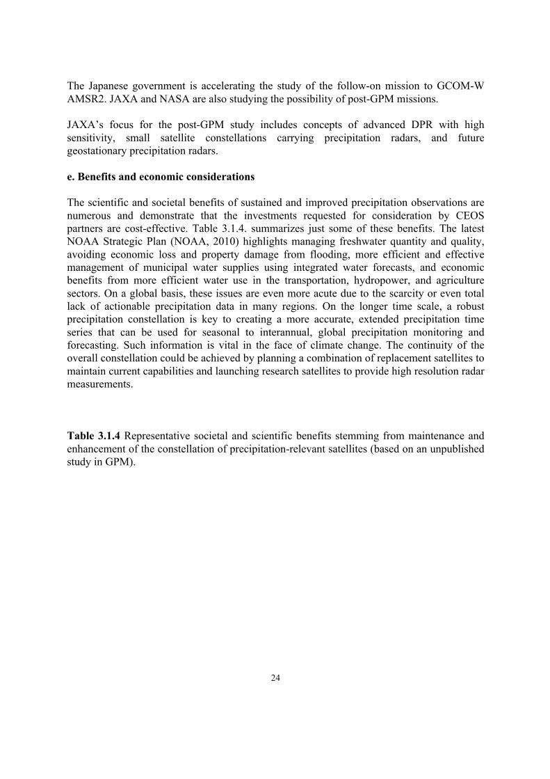
24
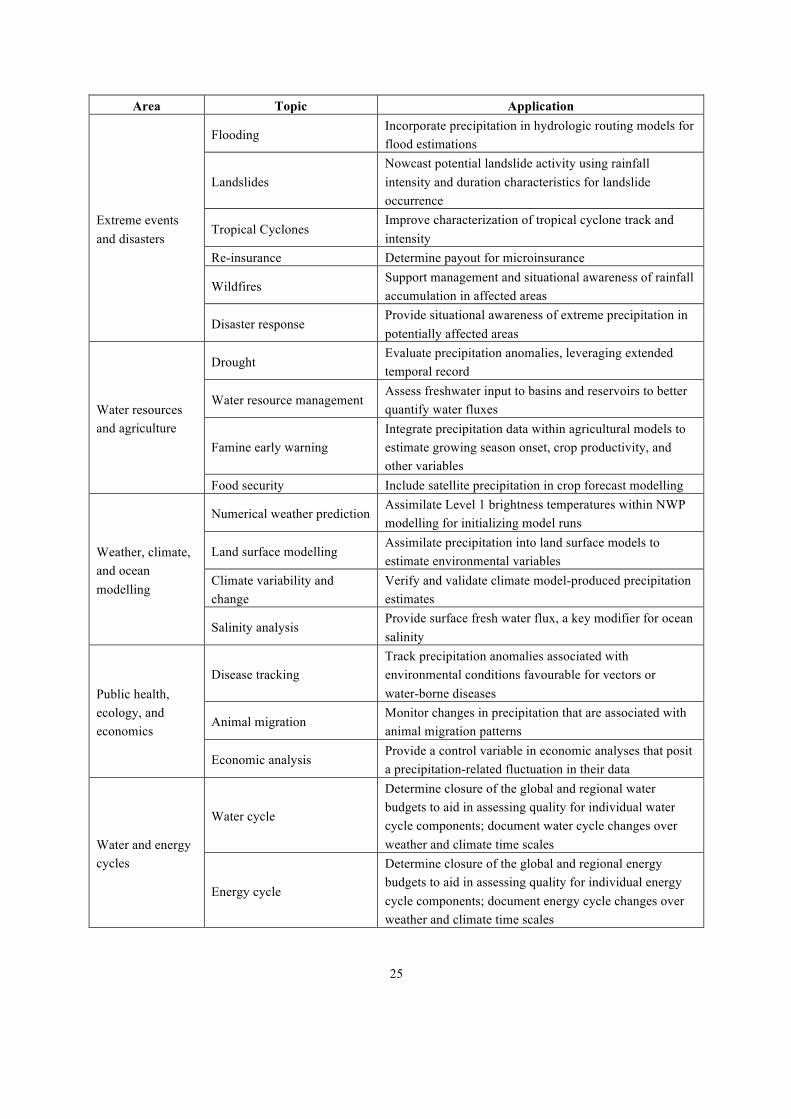
The Japanese government is accelerating the study of the follow-on mission to GCOM-W AMSR2. JAXA and NASA are also studying the possibility of post-GPM missions. JAXA’s focus for the post-GPM study includes concepts of advanced DPR with high sensitivity, small satellite constellations carrying precipitation radars, and future geostationary precipitation radars. e. Benefits and economic considerations The scientific and societal benefits of sustained and improved precipitation observations are numerous and demonstrate that the investments requested for consideration by CEOS partners are cost-effective. Table 3.1.4. summarizes just some of these benefits. The latest NOAA Strategic Plan (NOAA, 2010) highlights managing freshwater quantity and quality, avoiding economic loss and property damage from flooding, more efficient and effective management of municipal water supplies using integrated water forecasts, and economic benefits from more efficient water use in the transportation, hydropower, and agriculture sectors. On a global basis, these issues are even more acute due to the scarcity or even total lack of actionable precipitation data in many regions. On the longer time scale, a robust precipitation constellation is key to creating a more accurate, extended precipitation time series that can be used for seasonal to interannual, global precipitation monitoring and forecasting. Such information is vital in the face of climate change. The continuity of the overall constellation could be achieved by planning a combination of replacement satellites to maintain current capabilities and launching research satellites to provide high resolution radar measurements. Table 3.1.4 Representative societal and scientific benefits stemming from maintenance and enhancement of the constellation of precipitation-relevant satellites (based on an unpublished study in GPM).
25
Area Topic Application
Extreme events and disasters
Flooding Incorporate precipitation in hydrologic routing models for flood estimations
Landslides Nowcast potential landslide activity using rainfall intensity and duration characteristics for landslide occurrence
Tropical Cyclones Improve characterization of tropical cyclone track and intensity
Re-insurance Determine payout for microinsurance
Wildfires Support management and situational awareness of rainfall accumulation in affected areas
Disaster response Provide situational awareness of extreme precipitation in potentially affected areas
Water resources and agriculture
Drought Evaluate precipitation anomalies, leveraging extended temporal record
Water resource management Assess freshwater input to basins and reservoirs to better quantify water fluxes
Famine early warning Integrate precipitation data within agricultural models to estimate growing season onset, crop productivity, and other variables
Food security Include satellite precipitation in crop forecast modelling
Weather, climate, and ocean modelling
Numerical weather prediction Assimilate Level 1 brightness temperatures within NWP modelling for initializing model runs
Land surface modelling Assimilate precipitation into land surface models to estimate environmental variables
Climate variability and change
Verify and validate climate model-produced precipitation estimates
Salinity analysis Provide surface fresh water flux, a key modifier for ocean salinity
Public health, ecology, and economics
Disease tracking Track precipitation anomalies associated with environmental conditions favourable for vectors or water-borne diseases
Animal migration Monitor changes in precipitation that are associated with animal migration patterns
Economic analysis Provide a control variable in economic analyses that posit a precipitation-related fluctuation in their data
Water and energy cycles
Water cycle
Determine closure of the global and regional water budgets to aid in assessing quality for individual water cycle components; document water cycle changes over weather and climate time scales
Energy cycle
Determine closure of the global and regional energy budgets to aid in assessing quality for individual energy cycle components; document energy cycle changes over weather and climate time scales
26
3.2 Soil moisture Soil moisture plays important roles in climate and water resources management. In particular, it modifies the partitioning of incoming radiative energy into sensible and latent heat fluxes and the partitioning of precipitation between infiltration, runoff, and evaporation. Soil moisture must be accurately represented in hydrologic and land surface models because of its key role in environmental processes—for instance, in runoff generation during a precipitation event and, consequently, in flood forecasting. At climate time scales, soil moisture, together with sea surface temperatures, is a critical boundary condition controlling fluxes to the atmosphere (Seneviratne et al., 2010). Soil moisture is also a predictive factor for summer precipitation over continents in model experiments and has an effect on convective precipitation events over arid zones. In general, soil moisture becomes a critical forcing function for continental areas during the summer months, when potential evaporation rates are at a maximum but water availability is limited due to dry conditions. However, quantifying the importance of soil moisture in stimulating summer convection has been hampered by the lack of suitable long-term datasets with high-resolution observations both in time and space. For water management applications, the agricultural and forest communities are interested in soil moisture because it is critical for plant growth. The vigour and productivity of vegetation is determined by the rate at which plants accumulate mass, which depends on photosynthesis and transpiration rates, and which in turn is partly driven by the plants’ ability to rapidly access and uptake water. Soil moisture-vegetation-evaporation interactions form critical links between the water and carbon cycles. Agricultural communities therefore have a vested interest in accessing reliable soil moisture data, as it provides insight not only into vegetation health, but can also be used as a tool to effectively coordinate water and irrigation management. As a consequence of its influence on vegetation health, soil moisture also plays a significant role in the availability of fuel moisture in woody vegetation and therefore is also a critical variable in fire spread modelling, which supports a further focus on environmental hazard prediction. a. Confirmation of the validated requirements
GEO Water SBA requirements for soil moisture are provided in Table 3.2.1.

27
Table 3.2.1. GEO Water SBA requirements for soil moisture. Source: GEO task US-09-01a: Critical Earth Observations Priorities. Legend: L=Local, R=Regional, G=Global. Variable Horizontal
Resolution Time Resolution
Vertical Resolution
Accuracy Latency
Soil Moisture
L: 0.1 km to 1 km
L/R: 1 to 6 hrs (1-10 days for vadose zone)
10 cm Res. to 1 m depth; 30-100 cm for vadose zone or to depth of water table
0.02 m3/m3 or stated variably as 5 g/kg to 10 g/kg to 50 g/kg. Other units also used: Pascals, or cm/mm per 100 cms, or g/kg
Stated variably as NRT or 0.5 days to 1 day; 1-5 days to 10 d to 30 days to 144 days to 720 days (application dependent)
R: 10 km
R: 1-3 days to 1 week;
G: 50 to 100 km to 500 km
G: 1 to 30 days to 3 months for some applications
Also stated variably as 0.01 km to 250 km for some applications
The report Systematic Observation Requirements for Satellite-based Data Products for Climate, December 2010, GO’S-154 provides GCOS ECV soil moisture requirements; horizontal resolution (50 km), temporal resolution (daily), accuracy (0.04 m3/m3), and stability (0.01 m3/m3/year). The targets are set for an accuracy of about 10% of saturated moisture content and stability of about 2%of saturated moisture content. The report 2015 Update of CEOS-CGMS Actions in the Response to GCOS IP, May 2015 compares requirements and existing or planned capabilities of the observation system for the GCOS/ECV (see Appendix A). WMO-SOG-H indicates that none of the instruments provide a satisfactory combination of spatial resolution and repeat cycle (two to three days). AMSR data comes close to providing soil moisture or land wetness information that may be marginally useful for meso-scale modes, but data timeliness remain challenging. The ASCAT surface soil moisture product is the first truly operational satellite soil moisture product that may be used for NWP, flood forecasting, and other time-critical applications. The current soil moisture requirements are suited to climate users who want to estimate energy fluxes. However, many users in the agricultural sector are not satisfied with current soil moisture data because they do not represent soil moisture in the plant root or vadose zone. While these values can be estimated using models, there is always debate about how reliable the values are.
28
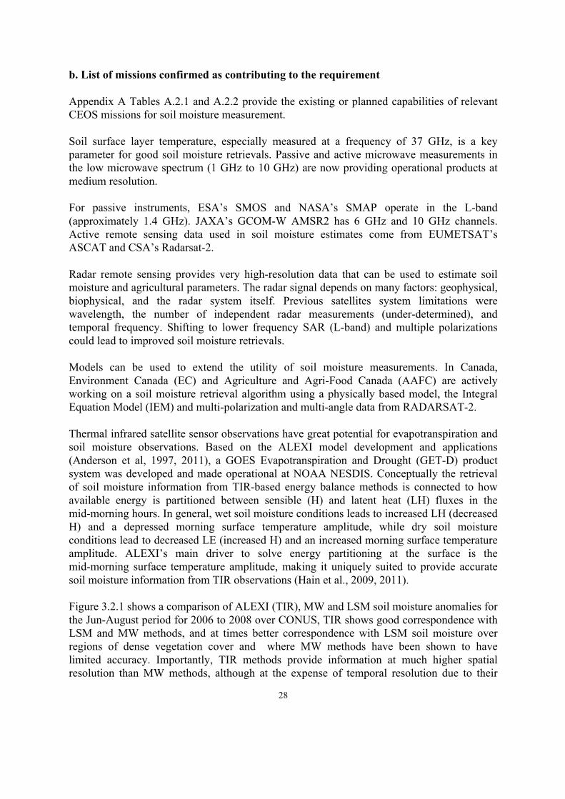
b. List of missions confirmed as contributing to the requirement Appendix A Tables A.2.1 and A.2.2 provide the existing or planned capabilities of relevant CEOS missions for soil moisture measurement. Soil surface layer temperature, especially measured at a frequency of 37 GHz, is a key parameter for good soil moisture retrievals. Passive and active microwave measurements in the low microwave spectrum (1 GHz to 10 GHz) are now providing operational products at medium resolution. For passive instruments, ESA’s SMOS and NASA’s SMAP operate in the L-band (approximately 1.4 GHz). JAXA’s GCOM-W AMSR2 has 6 GHz and 10 GHz channels. Active remote sensing data used in soil moisture estimates come from EUMETSAT’s ASCAT and CSA’s Radarsat-2. Radar remote sensing provides very high-resolution data that can be used to estimate soil moisture and agricultural parameters. The radar signal depends on many factors: geophysical, biophysical, and the radar system itself. Previous satellites system limitations were wavelength, the number of independent radar measurements (under-determined), and temporal frequency. Shifting to lower frequency SAR (L-band) and multiple polarizations could lead to improved soil moisture retrievals. Models can be used to extend the utility of soil moisture measurements. In Canada, Environment Canada (EC) and Agriculture and Agri-Food Canada (AAFC) are actively working on a soil moisture retrieval algorithm using a physically based model, the Integral Equation Model (IEM) and multi-polarization and multi-angle data from RADARSAT-2. Thermal infrared satellite sensor observations have great potential for evapotranspiration and soil moisture observations. Based on the ALEXI model development and applications (Anderson et al, 1997, 2011), a GOES Evapotranspiration and Drought (GET-D) product system was developed and made operational at NOAA NESDIS. Conceptually the retrieval of soil moisture information from TIR-based energy balance methods is connected to how available energy is partitioned between sensible (H) and latent heat (LH) fluxes in the mid-morning hours. In general, wet soil moisture conditions leads to increased LH (decreased H) and a depressed morning surface temperature amplitude, while dry soil moisture conditions lead to decreased LE (increased H) and an increased morning surface temperature amplitude. ALEXI’s main driver to solve energy partitioning at the surface is the mid-morning surface temperature amplitude, making it uniquely suited to provide accurate soil moisture information from TIR observations (Hain et al., 2009, 2011). Figure 3.2.1 shows a comparison of ALEXI (TIR), MW and LSM soil moisture anomalies for the Jun-August period for 2006 to 2008 over CONUS, TIR shows good correspondence with LSM and MW methods, and at times better correspondence with LSM soil moisture over regions of dense vegetation cover and where MW methods have been shown to have limited accuracy. Importantly, TIR methods provide information at much higher spatial resolution than MW methods, although at the expense of temporal resolution due to their
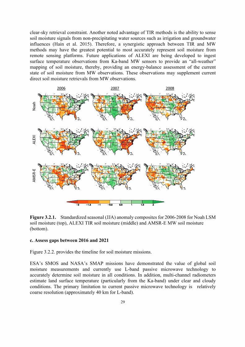
29
clear-sky retrieval constraint. Another noted advantage of TIR methods is the ability to sense soil moisture signals from non-precipitating water sources such as irrigation and groundwater influences (Hain et al. 2015). Therefore, a synergistic approach between TIR and MW methods may have the greatest potential to most accurately represent soil moisture from remote sensing platforms. Future applications of ALEXI are being developed to ingest surface temperature observations from Ka-band MW sensors to provide an “all-weather” mapping of soil moisture, thereby, providing an energy-balance assessment of the current state of soil moisture from MW observations. These observations may supplement current direct soil moisture retrievals from MW observations. Figure 3.2.1. Standardized seasonal (JJA) anomaly composites for 2006-2008 for Noah LSM soil moisture (top), ALEXI TIR soil moisture (middle) and AMSR-E MW soil moisture (bottom). c. Assess gaps between 2016 and 2021 Figure 3.2.2. provides the timeline for soil moisture missions. ESA’s SMOS and NASA’s SMAP missions have demonstrated the value of global soil moisture measurements and currently use L-band passive microwave technology to accurately determine soil moisture in all conditions. In addition, multi-channel radiometers estimate land surface temperature (particularly from the Ka-band) under clear and cloudy conditions. The primary limitation to current passive microwave technology is relatively coarse resolution (approximately 40 km for L-band).

30
NASA and ISRO are developing NISAR carrying L-band SAR and S-band SAR for planned launch in 2021. For passive instruments, there is no follow-on plan for SMOS and SMAP. JAXA is studying a GCOM-W AMSR2 follow-on. Considering the uncertainty of these instruments' operation in the year 2021, planning for these mission follow-ons should be reinforced. Figure 3.2.2. Soil moisture mission timeline. Figure 3.2.3. provides a soil moisture observation sampling analysis for 2016 and 2021 that considers SMOS, SMAP, GCOM-W, METOP-A, and METOP-B ASCAT. Comparing missions in 2016 and 2021, only SMOS (earliest launch date among the three missions) was excluded from the simulation. Since there are no confirmed follow-on plans for SMOS, SMAP, and GCOM-W, there is a considerable risk of gaps in 2021.
LST 2016 2017 2018 2019 2020 2021 2022 2023 2024 2025 2026 2027012345
6
78
9
10
1112
13
14
1516
17
18
19
20
21
222324
SMOS
SMAP
GCOM-W
METOP-AMETOP-B
Radasat-2
SAOCOM-1ASAOCOM-1B
Sentinel-1ASentinel-1B
MWIRadar
Planned Extended
GPM/GMI
NISAR

31
Figure 3.2 3. Soil moisture observation sampling analysis for 2016 and 2021. (Yamaji, 2016) d. Possible coordination of CEOS missions Coordination within confirmed missions: Follow-on missions of SMOS and SMAP should be studied. Addition of new missions: JAXA is studying the follow-on mission to GCOM-W AMSR2. JAXA and NASA are also studying a post-GPM mission that could provide relevant information for estimating soil moisture. Applications of SAR for estimating soil moisture should be promoted. e. Benefits and economic considerations
Soil moisture is an important state variable because it represents the driver for a number of physical processes, including runoff generation and evapotranspiration. Accurate soil moisture measurements provide the initial field assessments needed for improved precipitation and flood forecasts. Accurate measurement also provides valuable information for farmers wishing to assess their irrigation needs and for water resource managers who need to monitor drought conditions over large areas. The space-based measurement of soil moisture can follow two tracks: enhance the continuity of passive microwave measurements and better serve the community through the development of high resolution active sensors by enhancing research. Operational satellites can provide LST measurements that can in turn be used to soil moisture. This is the main input for many operational soil moisture products and the frequency and resolution of these measurements should be enhanced where possible. In many cases, this is a low-cost solution when it involves adding a microwave sensor to a mission whose collect data can help estimate a number of variables. As noted in the previous sections, however, soil moisture under cloud cover (where precipitation may also be occurring) is only available with active remote sensing; research missions and missions with active sensors with high resolution are therefore also needed. However the costs of these active measures would be much more

32
expensive than using the planned platforms and strengthening them by adding microwave sensors.

33
3.3 Evapotranspiration Evapotranspiration (ET) consists of processes of evaporation from soils and transpiration from plants (and plant canopies.) ET is the second-largest component (after precipitation) of the terrestrial water cycle at the global scale, and thus connects global energy and water cycles, since ET returns more than 60% of precipitation that falls on land back to the atmosphere. It is an important energy flux since land ET uses up more than half of the total solar energy absorbed by land surfaces. In semi-arid to arid systems, ET can account for over 90% of water loss. It is important to monitor ET fluxes to assess global climate change's impacts on ET. Although it is not considered as an ECV in the latest GCOS Implementation Plan, the GEOSS Water Strategy recognizes ET as an Essential Water Variable. ET is used for water management in agricultural systems. ET estimates can be applied to the assessment of water use in irrigation planning and monitoring. In some U.S. states, satellite ET maps are used to determine where irrigation has taken place and whether the insurance claims for crop losses caused by a lack of irrigation water are valid. However, ET modelling and remote sensing estimates at the continental and global scales need significant improvements to enable better water resources management, drought impact mitigation, and climate change adaptations. a. Confirmation of validated requirements The user requirements for ET provided in the GEO task report (GEO Task US-09-01a: Critical Earth Observations Priorities, Water Societal Benefit Area, GEO User Interface Committee, 2010) are given in Table 3.3.1. It should be noted that these requirements are for aggregated data products. Table 3.3.1. GEO Water SBA requirement for evapotranspiration Source: GEO task US-09-01a: Critical Earth Observations Priorities, Water Societal Benefit Area, GEO User Interface Committee, 2010. Variable Horizontal
Resolution Time Resolution
Vertical Resolution
Accuracy Latency
Evaporation/Evapotranspiration
L: 1 km 60 m (agriculture)
L: 1 to 6 hours 1-2 days (agriculture)
Surface (E), and LS vegetation cover or canopy height for ET
0.1 mm or 5%. Also stated in units of grams of H2O/m2/d
Generally not specified or RT (W/Precip) for point data assimilation and budget models
R: 10 km
R: 1 day
G: 50 to 100 km to 200 km
G: 1 day to 1 month
Despite the inability to measure evapotranspiration directly via remote sensing, it is nevertheless possible to measure states and processes that are needed to estimate evapotranspiration. More accurate estimation of evapotranspiration will require a new perspective on how multi-source measurements and models can be combined.
34
For ET, the 2007 NRC Decadal Survey recommended facilitating estimation of the diurnal cycle of evaporation over land and ocean surfaces with errors (at temporal resolutions sufficient to resolve the diurnal cycle) of less than 30 W/m2 at 10-km resolution, and over the open ocean with an accuracy of 5 W/m2 for spatial resolution of 1 degree (about 100 km). (Committee on Earth Science and Applications from Space: A Community Assessment and Strategy fro the Future, National Research Council, 2007)) Remote sensing of LST is critical to all current schemes for remotely estimating evapotranspiration. LST is directly related to the sensible heat component of the energy balance and is thus inversely proportional to latent energy and evaporation rates. Thermal remote sensing can provide an integrated look at land surface evaporation, although the choice of overpass times is critical for providing the most representative estimate (mid-afternoon radiant heating of the land surface provides the most useful signal). For some purposes, data obtained from geostationary satellites can also be used to derive LST and surface ET every hour under cloud-free conditions (this is a GEO Water SBA requirement). String synergies exist between ET and soil moisture in the physical system where, for a similar climate, ET rates tend to be correlated to soil moisture values. Furthermore methods such as ALEXI which has been developed to estimate ET can equally be used to estimate soil moisture as noted in Section 3.2. Participants at the 2015 Workshop on Evapotranspiration Mapping for Water Security held in Washington, DC recommended the time integration of ET for maps representing ET over daily, weekly, monthly, and longer time periods, based on ET obtained as “snapshots” determined on the day of a satellite overpass. Daily, weekly, monthly, and growing season ET maps are essential inputs to water resources management, water rights management, irrigation management, and hydrologic process modelling. ET "snapshots" require cloud-free image pixels. For spatial resolution, imagery collected in the visible and near-infrared wavelengths at 30 metres or finer spatial resolution, coupled with approximately 100 metres or finer thermal imagery, is required to produce ET information for individual fields where water is managed at the field level. The requirement to measure the effects of human activity on ET varies at the field level. ET measurements derived from satellite data at spatial resolutions greater than 100 metres are valuable for regional drought monitoring, hydrologic modelling, and other applications. The frequency of surface measurements is affected by cloud cover. When estimating ET over extended time periods, we need information for any one point every 32 days (at a minimum) to follow the evolution of vegetation and water availability. Field-scale ET mapping requires multiple Landsat-type satellites. Imaging every two days with eight 180 km Landsat satellites or four 360 km Landsat satellites can mitigate cloud cover by significantly increasing the probability of obtaining a cloud-free pixel value at least every 32 days (Allen, 2015). MODIS or Landsat data with one-day latency are not regularly available. USGS uses

35
four-hour latency for quick looks, with occasional delays. One-day latency is an acceptable and fair requirement. Programmes for the measurement of ET should explicitly analyse the trade-off between ET observations and modelling and evaluate in some detail whether different methods and data products might meet requirements better that single-approach satellites to meet the L, R, and G requirements. This is particularly relevant when looking at the two broad objectives: understanding the global terrestrial water cycle and providing useful information to water managers. Examples of ET measurements for climate purposes include those published in Raghuveer and Vinukollu, et al. (2011). Their article discusses three process-based approaches for estimating global evapotranspiration using multi-sensor remote sensing data. b. List of missions confirmed as contributing to the requirement
CEOS satellite missions relevant for ET are listed in Table 3.3.2. Table 3.3.2. Summarized observation capabilities of CEOS missions for estimating ET. Variable Horizontal
Resolution Time Resolution
Accuracy Latency
Evaporation/Evapotranspiration
GEO: 3-10 km MODIS: 1 km VIIRS: 750 m, 375 m Sentinel-3 SLSTR: 1 km
OLCI: 300 m GCOM-C/SGLI: 1 km, 250 m LANDSAT: 30 m, 100 m CBERS: 40 m, 80 m ISS/ECOSTRESS: 100 m
Sub-hourly Daily Daily Daily Daily 16 days 26 days Diurnal cycle
1 day
Missions such as ECOSTRESS, which provides field-scale ET data at different times of day from the International Space Station, provide the observations required to enhance our understanding of the evolution of ET throughout the day. Closing the water budget using only satellite data is possible, although the results are not entirely satisfactory. According to Rodell (2016), it is difficult to obtain ET satellite data accurate enough to close the water budget. Generally, ET estimates on a global basis have +/- 30% uncertainty. Figure 2.2. indicates that land data assimilation could be helpful for ET. We need to be able to rely on data assimilation systems for appropriate data outputs. The inputs must necessarily also be accurate in order to lead to reliable outputs. The data should also be cross-referenced
36
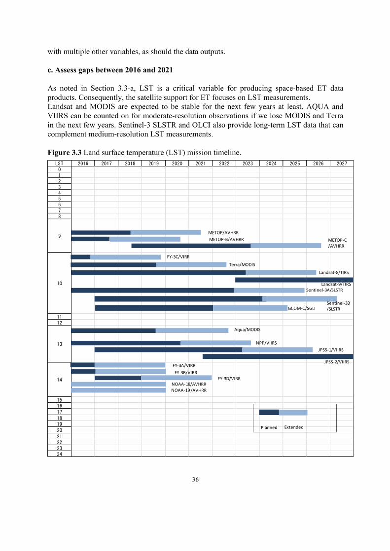
with multiple other variables, as should the data outputs. c. Assess gaps between 2016 and 2021 As noted in Section 3.3-a, LST is a critical variable for producing space-based ET data products. Consequently, the satellite support for ET focuses on LST measurements. Landsat and MODIS are expected to be stable for the next few years at least. AQUA and VIIRS can be counted on for moderate-resolution observations if we lose MODIS and Terra in the next few years. Sentinel-3 SLSTR and OLCI also provide long-term LST data that can complement medium-resolution LST measurements. Figure 3.3 Land surface temperature (LST) mission timeline.
LST 2016 2017 2018 2019 2020 2021 2022 2023 2024 2025 2026 2027012345678
9
10
1112
13
14
1516
17
1819
20
21222324
FY-3A/VIRRFY-3B/VIRR
FY-3C/VIRR
FY-3D/VIRR
METOP/AVHRRMETOP-B/AVHRR METOP-C
/AVHRR
NPP/VIIRS
NOAA-18/AVHRRNOAA-19/AVHRR
Planned Extended
JPSS-1/VIIRS
Terra/MODIS
Aqua/MODIS
Landsat-8/TIRS
Landsat-9/TIRS
JPSS-2/VIIRS
Sentinel-3A/SLSTR
Sentinel-3B/SLSTRGCOM-C/SGLI

37
d. Possible coordination of CEOS missions Improved coordination within confirmed missions: Coordination of CEOS LST missions (at high spatial or low temporal scale (LANDSAT), moderate spatial/temporal scale (MODIS), and low spatial/high temporal resolution (geostationary satellites) for data aquistion and data product generation would improve ET estimation from local to the global scale. CEOS LSI-VC is addressing this need. Addition of new missions : Responsible agencies need to process LST datasets from satellites and make them available so that the products can be used to map ET in near-real time. This would involve a higher revisit time (four days) for LST observations, which are needed at high resolutions (finer than 100 m) to compensate for data loss caused by cloud cover. This requires multiple LANDSAT-type satellites in orbit to provide imaging at a four-day revisit interval. e. Benefits and economic considerations The benefits of estimating and mapping ET related to its representation of vegetation vigour and growth. ET can be used to estimate crop and vegetation production and irrigation use. One example of savings caused by ET measurements comes from the state of Idaho, which has not hired any insurance inspectors because ET can be used to estimate water used for irrigation and to confirm or deny claims from farmers who say they did not receive an allocation of irrigation water in a given crop year. The increased capability of expanded monitoring and cost savings could be very extensive when aggregated through society. ET is not measured directly but is estimated from several measured variables including LST. A number of synergies exist between soil moisture and ET estimation because of the central nature of LAST estimates. It would seem reasonable to explore the design of a mission where the instruments needed for both variables could be measured at high resolution and frequency could be observed.

38
3.4 River discharge From a water management perspective, streamflow measurements are essential for designing and operating engineering works (dams, reservoirs, river regulation, etc.) because they provide various water-related services (navigation, flood protection, water supply for irrigation, municipal or industrial water use, and ecosystem management). Streamflow measurements also provide the knowledge required to promote healthy aquatic ecosystems. Extreme flow conditions (high or low flows) create requirements for more resilient water management infrastructures and management systems. Streamflow also serves as a medium for many biological and chemical processes and affects aquatic habitats and the sustainability of ecosystem services. From a scientific perspective, runoff and streamflow are important elements of the water cycle because they integrate across precipitation, evapotranspiration, soil moisture, and groundwater over a basin. River discharge measurements are a reliable basis for evaluating water cycle models. As a result, it is a very important variable to maintain for practical water and habitat management reasons and for use in calibrating and evaluating hydrological and coupled land-atmosphere models. Unfortunately, in-situ observations of discharge are presently lacking over significant portions of the Earth’s surface (Figure 3.4.1) because sharing of data collected at gauges is limited. Requirements for discharge measurements are provided in Table 3.4.1.
Figure 3.4.1. The global distribution of in-situ gauges for the important hydrologic measurement of river discharge is not uniform. Remote sensed measurements can complement this network to help fill gaps in current knowledge and future monitoring capacity.
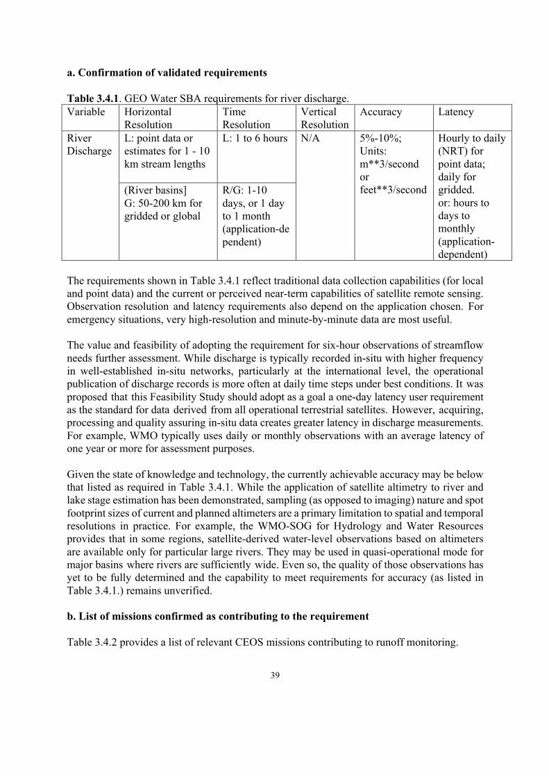
39
a. Confirmation of validated requirements Table 3.4.1. GEO Water SBA requirements for river discharge. Variable Horizontal
Resolution Time Resolution
Vertical Resolution
Accuracy Latency
River Discharge
L: point data or estimates for 1 - 10 km stream lengths
L: 1 to 6 hours
N/A 5%-10%; Units: m**3/second or feet**3/second
Hourly to daily (NRT) for point data; daily for gridded. or: hours to days to monthly (application- dependent)
(River basins] G: 50-200 km for gridded or global
R/G: 1-10 days, or 1 day to 1 month (application-dependent)
The requirements shown in Table 3.4.1 reflect traditional data collection capabilities (for local and point data) and the current or perceived near-term capabilities of satellite remote sensing. Observation resolution and latency requirements also depend on the application chosen. For emergency situations, very high-resolution and minute-by-minute data are most useful. The value and feasibility of adopting the requirement for six-hour observations of streamflow needs further assessment. While discharge is typically recorded in-situ with higher frequency in well-established in-situ networks, particularly at the international level, the operational publication of discharge records is more often at daily time steps under best conditions. It was proposed that this Feasibility Study should adopt as a goal a one-day latency user requirement as the standard for data derived from all operational terrestrial satellites. However, acquiring, processing and quality assuring in-situ data creates greater latency in discharge measurements. For example, WMO typically uses daily or monthly observations with an average latency of one year or more for assessment purposes. Given the state of knowledge and technology, the currently achievable accuracy may be below that listed as required in Table 3.4.1. While the application of satellite altimetry to river and lake stage estimation has been demonstrated, sampling (as opposed to imaging) nature and spot footprint sizes of current and planned altimeters are a primary limitation to spatial and temporal resolutions in practice. For example, the WMO-SOG for Hydrology and Water Resources provides that in some regions, satellite-derived water-level observations based on altimeters are available only for particular large rivers. They may be used in quasi-operational mode for major basins where rivers are sufficiently wide. Even so, the quality of those observations has yet to be fully determined and the capability to meet requirements for accuracy (as listed in Table 3.4.1.) remains unverified. b. List of missions confirmed as contributing to the requirement Table 3.4.2 provides a list of relevant CEOS missions contributing to runoff monitoring.
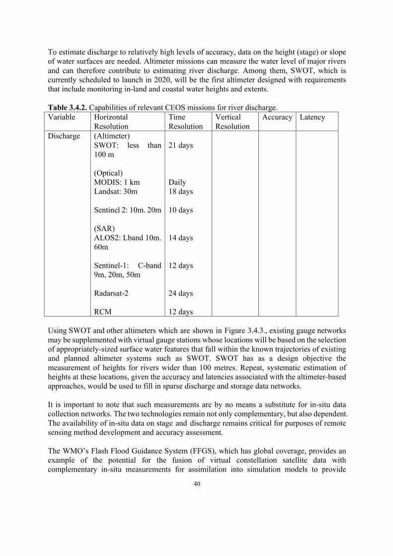
40
To estimate discharge to relatively high levels of accuracy, data on the height (stage) or slope of water surfaces are needed. Altimeter missions can measure the water level of major rivers and can therefore contribute to estimating river discharge. Among them, SWOT, which is currently scheduled to launch in 2020, will be the first altimeter designed with requirements that include monitoring in-land and coastal water heights and extents. Table 3.4.2. Capabilities of relevant CEOS missions for river discharge. Variable Horizontal
Resolution Time Resolution
Vertical Resolution
Accuracy Latency
Discharge (Altimeter) SWOT: less than 100 m (Optical) MODIS: 1 km Landsat: 30m Sentinel 2: 10m. 20m (SAR) ALOS2: Lband 10m. 60m Sentinel-1: C-band 9m, 20m, 50m Radarsat-2 RCM
21 days Daily 18 days 10 days 14 days 12 days 24 days 12 days
Using SWOT and other altimeters which are shown in Figure 3.4.3., existing gauge networks may be supplemented with virtual gauge stations whose locations will be based on the selection of appropriately-sized surface water features that fall within the known trajectories of existing and planned altimeter systems such as SWOT. SWOT has as a design objective the measurement of heights for rivers wider than 100 metres. Repeat, systematic estimation of heights at these locations, given the accuracy and latencies associated with the altimeter-based approaches, would be used to fill in sparse discharge and storage data networks. It is important to note that such measurements are by no means a substitute for in-situ data collection networks. The two technologies remain not only complementary, but also dependent. The availability of in-situ data on stage and discharge remains critical for purposes of remote sensing method development and accuracy assessment. The WMO’s Flash Flood Guidance System (FFGS), which has global coverage, provides an example of the potential for the fusion of virtual constellation satellite data with complementary in-situ measurements for assimilation into simulation models to provide
41
decision support. Flash floods are among the world’s deadliest natural disasters, with an average of more than 5,000 lives lost annually and significant detrimental social, economic, and environmental impacts. Accounting for approximately 85% of flooding cases, flash floods also have the highest mortality rate (defined as the number of deaths per number of people affected) among different classes of flooding (e.g., riverine and coastal). Urban areas are particularly sensitive to heavy rain events due to the large proportion of the area that is covered with impervious surfaces and the tendency in some cities to offer little or no storm drainage. Hence, WMO is implementing the FFGS in technical cooperation with the Hydrologic Research Centre (HRC) in San Diego, California and with financial support from USAID. It is expected that the system’s coverage will reach over 1 billion people by mid-2017. Through a regional implementation approach, the main objective of the FFGS is to reduce vulnerability to hydrometeorological disasters, specifically flash floods, by developing and implementing flash flood guidance systems that provide timely and accurate flash flood warnings. An important and innovative characteristic of the FFGS is the integration of multiplatform observations, including satellite-based data on precipitation, soil moisture, and land cover, in-situ observations, and other static databases, as drivers in a multi-model-based computational core that can calculate a number of warning products at the local scale. Technical elements of the FFGS include the operational use of bias-corrected satellite precipitation fields and physically-based hydrologic modelling to determine flash flood guidance and flash flood threat. Real-time estimates of high-resolution satellite precipitation data are routinely available globally on an hourly basis (see section 3.1-b) and can be integrated with real-time ground radar and in-situ observations (where available). Operational satellite-based soil moisture observations are ready to be integrated in the overall system in support of the physically based soil moisture accounting models (se section 3.2-b). The system allows the National Hydrological and Meteorological Services (NMHs) to use local nowcast/short-term-forecast methods to issue warnings, including local forecaster adjustments. The system provides flash flood information over lead time scales from three to six hours and for basins on the order of 100 km2. The FFGS by itself is a diagnostic tool. However, forecasting is afforded through the application of numerical weather prediction models to result in the extension of flash flood threat prediction to 48 hours. More information on the FFGS can be obtained here: http://www.wmo.int/ffgs and http://www.hrcwater.org. The WSIST’s assessment of requirements identified an additional aspect of river water flow for which satellite remote sensing is extremely well-suited and information is critically needed: flood extent, or the land surface area inundated by river flood waters. River flood extent, not discharge per se, is vitally important information in the cases of flood mitigation and response. Irrespective of the availability of river discharge data, in the event of flooding, timely information on the extent of floodwaters can greatly improve the safety and effectiveness of mitigation and rescue operations. Following flood events, information on flood extent can be used to more accurately assess damages and target recovery resources. Floods create conditions during which in-situ measurements are generally inadequate, reinforcing the need for remotely sensed information. The need for high temporal resolution is greatest in the case of floods. Several satellite-based methods are available on demand to map the extent of flooding in floodplains or large riverine systems and the flooding duration. These methods include visual, infrared, and radar sensors. And some satellites are especially useful for
42
mapping flood extent on a daily basis. For example, MODIS provides flood information at a spatial resolution of 250 metres on (potentially) a daily basis in the form of rapid response data provided by NASA’s LANCE system. Several satellite-based methods using data from optical, infrared, and radar sensors are available to map flooding extent and duration in floodplains or large riverine systems. Spatial resolution requirements are less stringent than those for discharge, while in the case of disaster response in particular, short latency is of critical importance. Advances in data-sharing achieved through the development of an international charter for disaster response provide an example (see https://www.disasterscharter.org/web/guest/home). However, shortcomings in data processing requirements during disaster events continue to challenge response effort effectiveness, pointing to the need to develop data creation and distribution systems that share value-added products (analysis-ready data) to user communities that lack extensive remotely sensed data processing resources or exploitation experience. c. Assess gaps between 2016 and 2021
Useful space-based measurements are expected to be about the same in 2021 as they are now. However, some missions will be more specifically directed at streamflow measurement (e.g., SWOT). Unfortunately, the 21-day repeat timeframe associated with the SWOT system falls well below confirmed sub-monthly temporal resolution requirements, but will nevertheless be useful for many applications including water resources assessment and the sub-seasonal variability of water resources availability.. To estimate discharge with high levels of accuracy, stage has been measured in-situ and used in combination with in-situ-measured volume, velocity, and channel hydraulic characteristics (for example, channel bottom shape and roughness) for the determination of the stage-discharge relationship at the gauging site (rating curve). The current inability to reliably measure channel hydraulic characteristics such as bathymetry, particularly in the case of turbid waters or canopy-obscured channels, represents a major information gap. The increased availability of remotely sensed data from optical, polarimetric radar, and altimeters will contribute to the continued development of relationships between observable variables and necessary channel parameters. The development of new systems should be based on the recognition that satellite and in-situ observations complement one another (as opposed to being competitive). The altimeter mission timeline is given in Figure 3.4.3. From the satellite observation point of view, revisit time is an issue. Spatial resolution of the altimeter missions other than SWOT are also an issue.
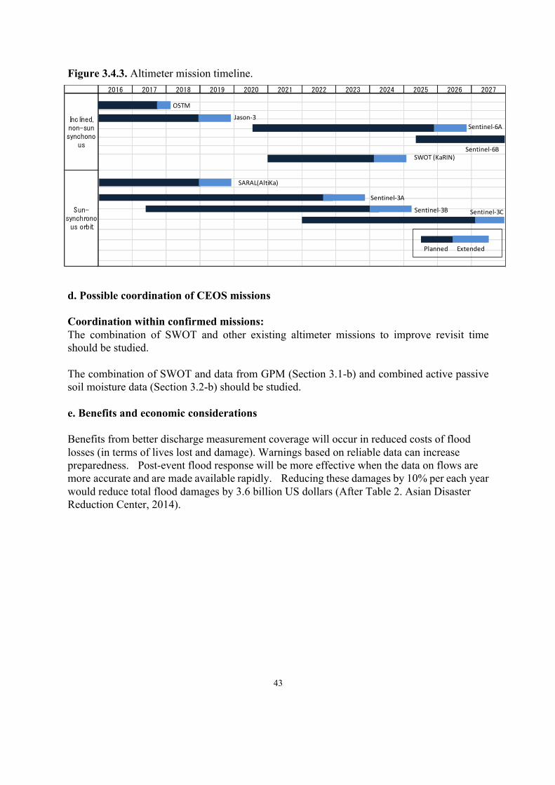
43
Figure 3.4.3. Altimeter mission timeline. d. Possible coordination of CEOS missions Coordination within confirmed missions: The combination of SWOT and other existing altimeter missions to improve revisit time should be studied.
The combination of SWOT and data from GPM (Section 3.1-b) and combined active passive soil moisture data (Section 3.2-b) should be studied. e. Benefits and economic considerations Benefits from better discharge measurement coverage will occur in reduced costs of flood losses (in terms of lives lost and damage). Warnings based on reliable data can increase preparedness. Post-event flood response will be more effective when the data on flows are more accurate and are made available rapidly. Reducing these damages by 10% per each year would reduce total flood damages by 3.6 billion US dollars (After Table 2. Asian Disaster Reduction Center, 2014).
2016 2017 2018 2019 2020 2021 2022 2023 2024 2025 2026 2027
Inclined,non-sunsynchono
us
Sun-synchronous orbit
OSTM
Planned Extended
Jason-3Sentinel-6A
Sentinel-6B
SARAL(AltiKa)
Sentinel-3A
Sentinel-3B Sentinel-3C
SWOT (KaRIN)

44
3.5 Surface water storage Water stored on the land surface influences the flux of water from the land surface to the atmosphere, the infiltration of water to deep soil moisture and groundwater layers, and the runoff of water into the stream network. Over 2% of the land surface is covered by lakes and other water bodies (Lehner and Doll, 2004), which evaporate significant amounts to the atmosphere, especially in late summer and fall. These water bodies provide habitats that ensure biodiversity and serve as primary freshwater sources for humans. Changes in natural surface water storage provide important indicators of underlying hydrological processes due to natural or human-induced changes. The largest storage features are often well-monitored and regulated, but the exchange of information useful for global- and regional-scale (particularly transboundary) modelling and resource management is lacking. These data are often considered proprietary and are usually not shared. Water storage in lakes, rivers, floodplains, and wetlands are particularly poorly monitored. High-spatial resolution satellite remote sensing of surface water area and stage, when combined with information on elevation and bathymetry, make it possible to estimate changes in water volume in these features. Water in the form of snow and glacier is stored on the land surface and is part of the surface water storage that is available for use in agriculture and the domestic water supply. At more northern latitudes, snow is critical because it provides the spring moisture that is used in agriculture and to meet other water supply needs. Snow Water Equivalent (SWE) is used to represent the moisture available in the snow pack. At mid and high latitudes, the snow that accumulates in mountains provides much of the water used to irrigate crops during the growing season. Consequently, SWE measurements are extremely useful for predicting spring and summer water supplies and flood potential in these areas. Ground ice reduces the infiltration into and the migration of water through soils, reduces the amount of water that can be stored in soils, and increases the runoff generated from melting snow. Seasonally and permanently frozen lands also are very sensitive to climate change because warming affects wetland patterns, methane gas releases, slumping and disruptions to infrastructure, as well as transport and access, among other hazards and costs. In addition, monitoring the trend and rate of mountain glacier retreat is important for assessing the impacts of climate change and predicting its potential long-term effects on the availability of freshwater in the summer months. a. Confirmation of validated requirements The GEO Water SBA requirements for surface water storage are shown in Table 3.5.1.
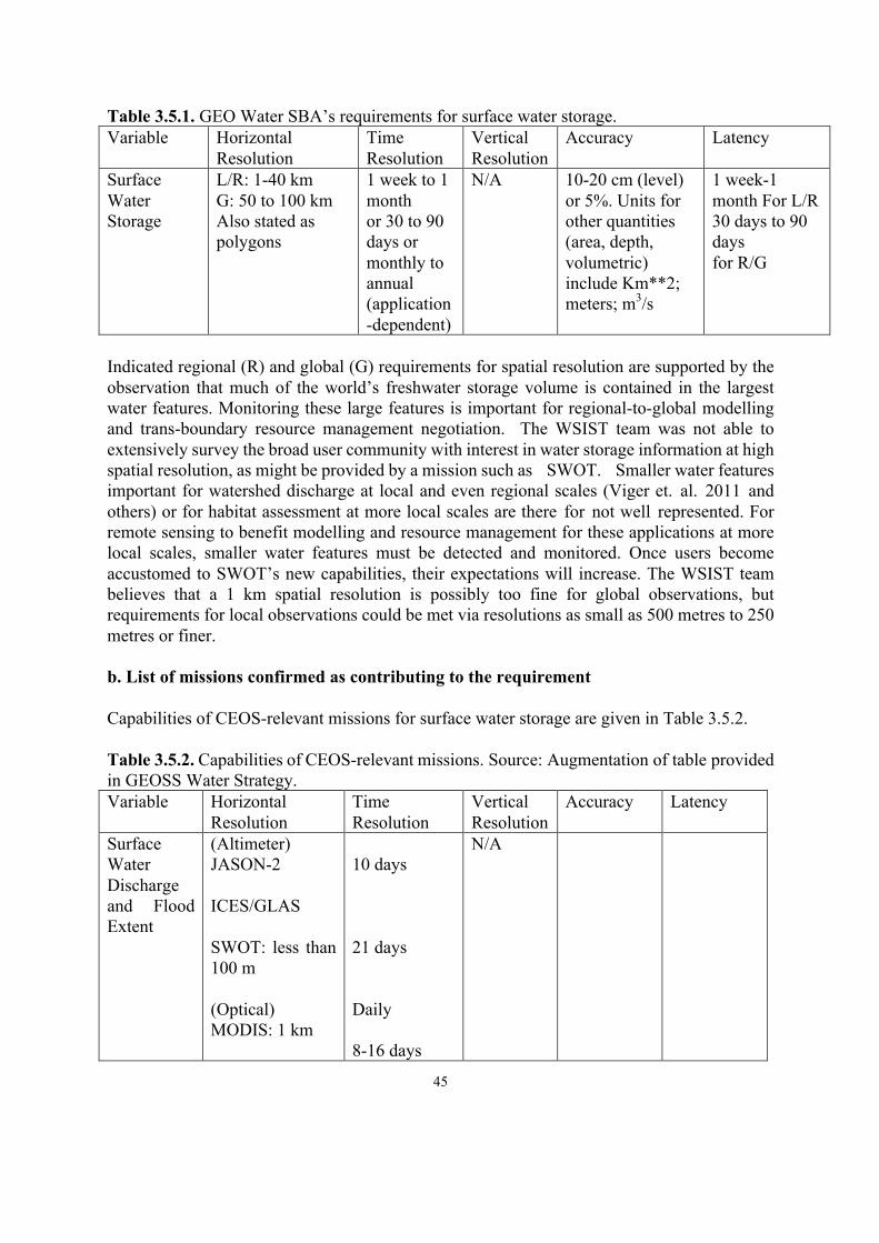
45
Table 3.5.1. GEO Water SBA’s requirements for surface water storage. Variable Horizontal
Resolution Time Resolution
Vertical Resolution
Accuracy Latency
Surface Water Storage
L/R: 1-40 km G: 50 to 100 km Also stated as polygons
1 week to 1 month or 30 to 90 days or monthly to annual (application-dependent)
N/A 10-20 cm (level) or 5%. Units for other quantities (area, depth, volumetric) include Km**2; meters; m3/s
1 week-1 month For L/R 30 days to 90 days for R/G
Indicated regional (R) and global (G) requirements for spatial resolution are supported by the observation that much of the world’s freshwater storage volume is contained in the largest water features. Monitoring these large features is important for regional-to-global modelling and trans-boundary resource management negotiation. The WSIST team was not able to extensively survey the broad user community with interest in water storage information at high spatial resolution, as might be provided by a mission such as SWOT. Smaller water features important for watershed discharge at local and even regional scales (Viger et. al. 2011 and others) or for habitat assessment at more local scales are there for not well represented. For remote sensing to benefit modelling and resource management for these applications at more local scales, smaller water features must be detected and monitored. Once users become accustomed to SWOT’s new capabilities, their expectations will increase. The WSIST team believes that a 1 km spatial resolution is possibly too fine for global observations, but requirements for local observations could be met via resolutions as small as 500 metres to 250 metres or finer. b. List of missions confirmed as contributing to the requirement Capabilities of CEOS-relevant missions for surface water storage are given in Table 3.5.2. Table 3.5.2. Capabilities of CEOS-relevant missions. Source: Augmentation of table provided in GEOSS Water Strategy. Variable Horizontal
Resolution Time Resolution
Vertical Resolution
Accuracy Latency
Surface Water Discharge and Flood Extent
(Altimeter) JASON-2 ICES/GLAS SWOT: less than 100 m (Optical) MODIS: 1 km
10 days 21 days Daily 8-16 days
N/A
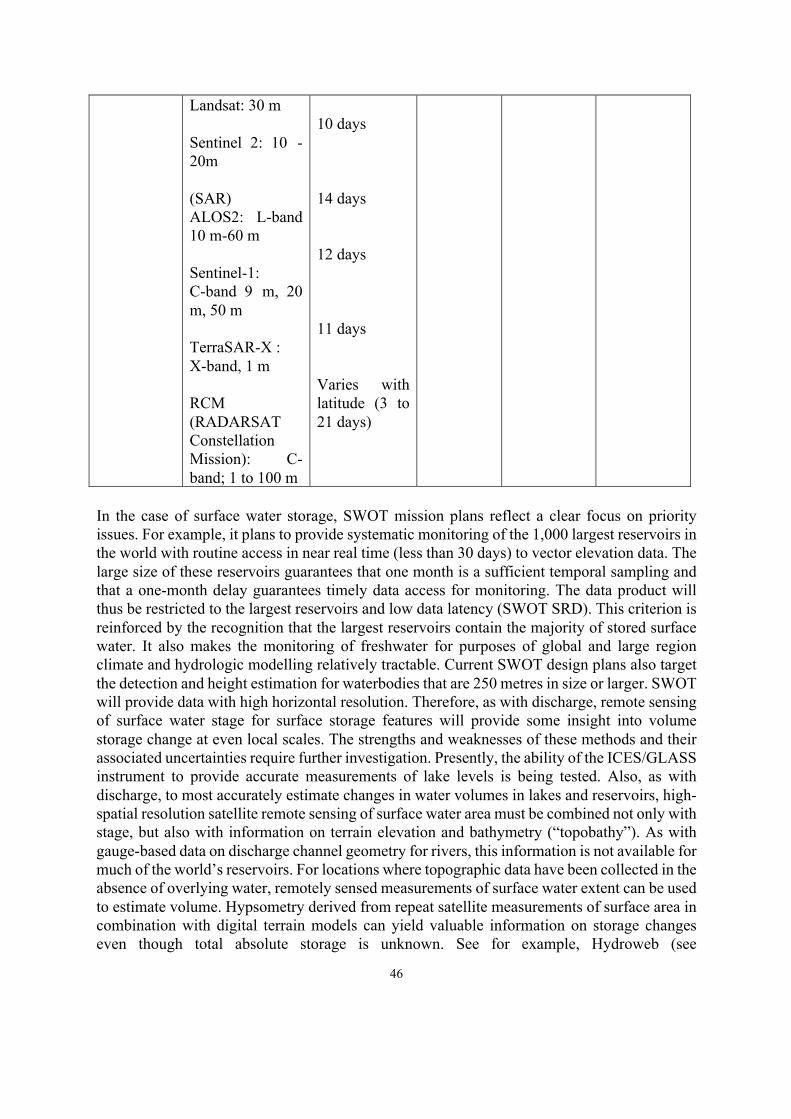
46
Landsat: 30 m Sentinel 2: 10 - 20m (SAR) ALOS2: L-band 10 m-60 m Sentinel-1: C-band 9 m, 20 m, 50 m TerraSAR-X : X-band, 1 m RCM (RADARSAT Constellation Mission): C- band; 1 to 100 m
10 days 14 days 12 days 11 days Varies with latitude (3 to 21 days)
In the case of surface water storage, SWOT mission plans reflect a clear focus on priority issues. For example, it plans to provide systematic monitoring of the 1,000 largest reservoirs in the world with routine access in near real time (less than 30 days) to vector elevation data. The large size of these reservoirs guarantees that one month is a sufficient temporal sampling and that a one-month delay guarantees timely data access for monitoring. The data product will thus be restricted to the largest reservoirs and low data latency (SWOT SRD). This criterion is reinforced by the recognition that the largest reservoirs contain the majority of stored surface water. It also makes the monitoring of freshwater for purposes of global and large region climate and hydrologic modelling relatively tractable. Current SWOT design plans also target the detection and height estimation for waterbodies that are 250 metres in size or larger. SWOT will provide data with high horizontal resolution. Therefore, as with discharge, remote sensing of surface water stage for surface storage features will provide some insight into volume storage change at even local scales. The strengths and weaknesses of these methods and their associated uncertainties require further investigation. Presently, the ability of the ICES/GLASS instrument to provide accurate measurements of lake levels is being tested. Also, as with discharge, to most accurately estimate changes in water volumes in lakes and reservoirs, high- spatial resolution satellite remote sensing of surface water area must be combined not only with stage, but also with information on terrain elevation and bathymetry (“topobathy”). As with gauge-based data on discharge channel geometry for rivers, this information is not available for much of the world’s reservoirs. For locations where topographic data have been collected in the absence of overlying water, remotely sensed measurements of surface water extent can be used to estimate volume. Hypsometry derived from repeat satellite measurements of surface area in combination with digital terrain models can yield valuable information on storage changes even though total absolute storage is unknown. See for example, Hydroweb (see
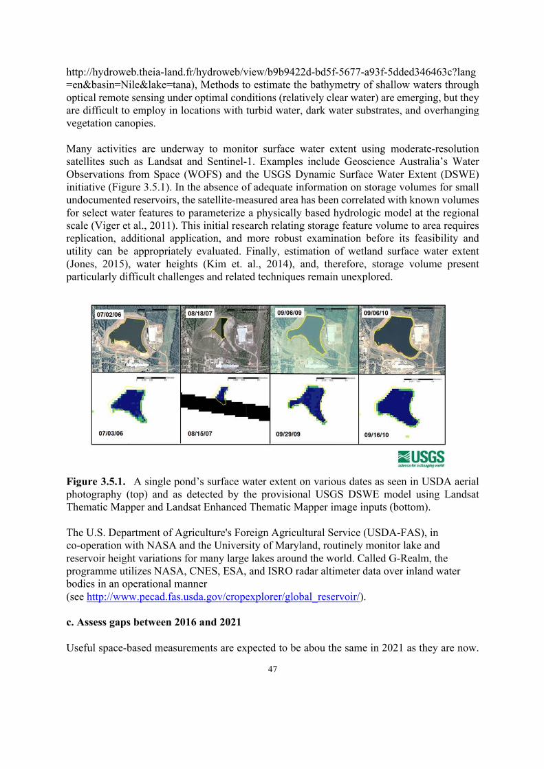
47
http://hydroweb.theia-land.fr/hydroweb/view/b9b9422d-bd5f-5677-a93f-5dded346463c?lang=en&basin=Nile&lake=tana), Methods to estimate the bathymetry of shallow waters through optical remote sensing under optimal conditions (relatively clear water) are emerging, but they are difficult to employ in locations with turbid water, dark water substrates, and overhanging vegetation canopies. Many activities are underway to monitor surface water extent using moderate-resolution satellites such as Landsat and Sentinel-1. Examples include Geoscience Australia’s Water Observations from Space (WOFS) and the USGS Dynamic Surface Water Extent (DSWE) initiative (Figure 3.5.1). In the absence of adequate information on storage volumes for small undocumented reservoirs, the satellite-measured area has been correlated with known volumes for select water features to parameterize a physically based hydrologic model at the regional scale (Viger et al., 2011). This initial research relating storage feature volume to area requires replication, additional application, and more robust examination before its feasibility and utility can be appropriately evaluated. Finally, estimation of wetland surface water extent (Jones, 2015), water heights (Kim et. al., 2014), and, therefore, storage volume present particularly difficult challenges and related techniques remain unexplored. Figure 3.5.1. A single pond’s surface water extent on various dates as seen in USDA aerial photography (top) and as detected by the provisional USGS DSWE model using Landsat Thematic Mapper and Landsat Enhanced Thematic Mapper image inputs (bottom). The U.S. Department of Agriculture's Foreign Agricultural Service (USDA-FAS), in co-operation with NASA and the University of Maryland, routinely monitor lake and reservoir height variations for many large lakes around the world. Called G-Realm, the programme utilizes NASA, CNES, ESA, and ISRO radar altimeter data over inland water bodies in an operational manner (see http://www.pecad.fas.usda.gov/cropexplorer/global_reservoir/). c. Assess gaps between 2016 and 2021 Useful space-based measurements are expected to be abou the same in 2021 as they are now.

48
However, some missions will be more specifically directed at surface water storage measurements (e.g., SWOT). (see Section 3.4-c) d. Possible coordination of CEOS missions As with other EWVs, the fusion of optical and radar systems for the purpose of surface water storage monitoring is at the experimental stage. It will continue to mature along with the greater availability of radar data to complement freely available data from optical systems such as Landsat and Sentinel. The combined use of these data sources to estimate surface water extent improves temporal resolution and helps overcome impacts of cloud cover on optical sensing systems. The goal for data producers is to fill observational gaps using different observational methods to yield the best product possible. As a first step, it is important to determine what gains in accuracy and services can be obtained from better coordination among confirmed and existing missions. e. Benefits and economic considerations Determining water storage is important for assessments and management. For example, monitoring wetlands is important for the Ramsar convention and Target 6.6 of the UN Sustainable Development Goals. There are also significant benefits for water resource management and assessment and SWOT offers an excellent opportunity for developing its capability. It is recommended that CEOS agencies support this mission.
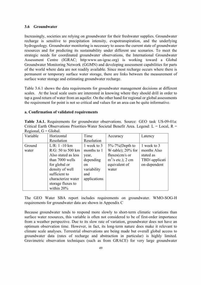
49
3.6 Groundwater Increasingly, societies are relying on groundwater for their freshwater supplies. Groundwater recharge is sensitive to precipitation intensity, evapotranspiration, and the underlying hydrogeology. Groundwater monitoring is necessary to assess the current state of groundwater resources and for predicting its sustainability under different use scenarios. To meet the strategic needs for coordinated groundwater observations, the International Groundwater Assessment Centre (IGRAC; http:www.un-igrac.org) is working toward a Global Groundwater Monitoring Network (GGMN) and developing assessment capabilities for parts of the world where data are not readily available. Since most recharge occurs where there is permanent or temporary surface water storage, there are links between the measurement of surface water storage and estimating groundwater recharge. Table 3.6.1 shows the data requirements for groundwater management decisions at different scales. At the local scale users are interested in knowing where they should drill in order to tap a good return of water from an aquifer. On the other hand for regional or global assessments the requirement for point is not so critical and values for an area can be quite informative. a. Confirmation of validated requirements Table 3.6.1. Requirements for groundwater observations. Source: GEO task US-09-01a: Critical Earth Observations Priorities-Water Societal Benefit Area. Legend: L = Local, R = Regional, G = Global. Variable Horizontal
Resolution Time Resolution
Accuracy Latency
Ground water
L/R: 1 -10 km R/G: 50 to 500 km Also stated as less than 7000 wells for global or density of well sufficient to characterize water storage fluxes to within 20%
1 week to 3 months to 1 year, depending on variability and applications
5%-7%(Depth to W-table); 20% for fluxes(cm/s or m3/s etc.); 2 cm equivalent of water
1 week to 3 months Also stated as TBD/-application-dependent
The GEO Water SBA report includes requirements on groundwater. WMO-SOG-H requirements for groundwater data are shown in Appendix C Because groundwater tends to respond more slowly to short-term climatic variations than surface water resources, this variable is often not considered to be of first-order importance from a weather perspective. Due to its slow rate of variation, groundwater does not have an optimum observation time. However, in fact, its long-term nature does make it relevant to climate scale analyses. Terrestrial observations are being made but overall global access to groundwater data (rates of recharge and abstraction in particular) is highly limited. Gravimetric observation techniques (such as from GRACE) for very large groundwater

50
bodies are available through data assimilation systems but require integration with higher-resolution and lower latency data in order to be useful for operational applications. IGRAC, a collaborative UNESCO/WMO centre, maintains a groundwater monitoring metadata and data system and contributes to the GEO Water Task. Due to the difficulty of obtaining groundwater data, IGRAC has established the GGMN. The GGMN consists of groundwater specialists who are members of a people network and can bring national data to problems. b. Define a list of missions confirmed as contributing to the requirement Capabilities of GRACE, GRACE FO, and GRACE-II are provided in Appendix A. Table 3.6.2. provides GRACE and GRACE-FO capabilities. Table 3.6.2. Observation capabilities of GRACE and GRACE-FO. Source: GEOSS Water Strategy Variable Horizontal
Resolution Time Resolution
Accuracy Latency
Groundwater
400 km
1 cm
The GRACE satellite’s resolution is no better than 150,000 km2 at mid-latitudes; the stated requirement is 1 km2 for individual aquifers. Although the satellite capability is far lower than horizontal resolution requirements, it should be noted that many regional requirements can be met with data at the current GRACE resolution. GRACE data used for drought monitoring show that these data are related to soil moisture, ET, and vegetation anomalies. Groundwater can be linked with soil moisture and ET through LDAS. The issue of data latency is being addressed to some degree. A GRACE quick-look product that is expected to have a two-week latency period, compared with the two- to four-month latency of the standard products, is being developed. GRACE FO has established an application development team. This team is considering applications such as the inter-decadal changes arising from climate change and the over-pumping of groundwater aquifers. INSAR measurements can provide high-spatial resolution information on land subsidence and hence groundwater extraction but they cannot provide a complete measurement of the groundwater signal because aquifer compaction is not elastic. c. Assess gaps between 2016 and 2021 Figure 3.6.1 shows mission timelines for GRACE and GRACE-FO based on the latest information.

51
Figure 3.6.1. Gravity mission timeline. Courtesy of Matt Rodell, NASA. The mission chart shows that GRACE is in service in 2016 and that GRACE Follow-On will be launched in early 2018. GRACE FO will have a laser-ranging system in addition to the standard microwave system for changes in the distance to measure range change between the two satellites, which is the key measurement. The configuration, however, will be nearly identical to the current GRACE mission and will be at an altitude of 500 km in non-sun synchronous orbit (CEOS EO DB). GRACE will survive no longer than the end of 2017 and there will therefore be a gap between GRACE and GRACE FO, but efforts are being made to minimize the effect of such a gap. GRACE-II is now being proposed to the Decadal Survey committee for launch sometime in the late 2020s or early 2030s. Such a mission will be critical for preserving continuity of the climate data records provided by the GRACE series of missions. In urban areas, the chance for water infiltration is minimal due to buildings, impervious surfaces, and the storm systems that remove the water before it has a chance to infiltrate the soil. There is a great need for groundwater data in urban environments to better understand its role in that environment. d. Possible coordination of CEOS missions Coordination within confirmed missions: CEOS should encourage space agencies to minimizing the impact of the mission gap between GRACE and GRACE FO. Addition of new missions: A proposed NASA/Germany GRACE-II mission for the Decadal Survey should be supported by international research communities and user communities, including GEO. The launch of additional gravimetric missions by other space agencies would create synergies that could potentially increase the spatial resolution and accuracy of the resulting data products. This possibility should be promoted by CEOS. It should be noted that it is more challenging to develop synergistic missions with groundwater than with many other measurements because of the focus on gravimetric measurements. This
2016 2017 2018 2019 2020 2021 2022 2023 2024 2025 2026 2027
G RAC E
G RAC E FO
G RAC E-II
GRACE
consideredbyDSforoperation 2027-2032
Planned Extended
GRACEFO
GRACEII

52
unique signal which represents variations in the gravity field gives a measure through a column and is not always correlated to the emission from a thin layer of soil or atmosphere. This is an area in which LDAS needs to play a major role in bringing datasets from various sources together.
e. Benefits and economic considerations
Groundwater measurements from GRACE have been instrumental in identifying regions where withdrawals from aquifers for irrigation are non-sustainable. Satellite data is the only source of geospatial coverage for all countries because few data are shared between countries making it impossible to provide a geospatial consideration of the water cycle.
53
4. Priority water cycle variable synergistic observation feasibility 4.1 Define synergistic observation requirements for high-priority parameters
Throughout the following discussions, references will be made to models as well as observational systems. Models play an increasingly important role in the delivery of information to users. In cases where observational systems are too degraded by budget reductions and satellites do not provide sufficient coverage models can be used to derive desired values from the larger scale environmental conditions that are measured. For example at northern latitudes the official meteorological observational systems struggle to provide a full representation of precipitation. Measurements in these regions are based on fewer and fewer observations. In these cases models which process the temperature, humidity, pressure and vertical velocity fields are able to produce precipitation patterns which may be as accurate as anything that can be derived from observations. Models also provide values for unmeasured values in the case of root zone soil moisture and other subsurface estimates when measurements are not possible. Scaling up (aggregation) and scaling down (disaggregation) are made possible through the use of models. In the data assimilation mode, models can bring together a wide range of observations from different times and space resolutions to produce accurate field representation. Other model applications involve providing information through diagnostic and predictive applications. A number of benefits arise from bringing precipitation and soil moisture measurements together in a more coordinated way. Precipitation and soil moisture data can be used together to address specific needs, such as: Precipitation in numerical weather prediction models: The prediction of precipitation is difficult to achieve in models, in part because precipitation processes are very difficult to represent in a numerical model. This difficulty arises from the plethora of interactions in the air column where the precipitation is forming. Current prediction techniques rely on bulk characteristics of the atmosphere, including the instability in the air column, the amount of moisture in the air column, and the amount of water being supplied to the air column by the underlying surface. Over land, this last variable is often addressed by using a land surface data assimilation system that can intake data on surface wetness in terms of vegetation and soil moisture. The assimilation system can take advantage of the correlations that have been demonstrated between the surface moisture and the intensity of the rain events that occur. Prediction models run on a six-hour cycle; consequently, it is important to update the information on this cycle. Data assimilation systems offer the opportunity to provide input on a less regular basis since they accumulate the information over a time interval and then produce the fields when they are required. Prediction of the flood potential from a rain event: heavy rain events are a common cause of floods, particularly at mid and equatorial latitudes. When the surface is saturated, the rain does not have the opportunity to infiltrate the soil and tends to run off. When all of the rain from a heavy rain event runs off, it overloads the storm sewage systems and other infrastructure put in place to deal with floods and can create very dangerous situations.

54
4.1.1 Options for meeting more of precipitation requirements when complementing the
precipitation parameter measurements with other parameter measurements The SMAP best-estimate analysis is produced approximately two-and-a-half days after real time due to the delay in the CPC Unified global gauge product. SMAP does not meet the requirements for data latency of one day. Improvements in data latency are needed for both precipitation and soil moisture. SMAP data have been used to estimate rainfall based on the work of Luca Brocca of the Italian Research Institute for Geo-Hydrological Protection. The soil water balance is solved during rain events. SMAP retrievals (as well as SMOS and ASTER soil moisture retrievals) show large increases during heavy rain events but they change more slowly as the soil slowly dries out under no or light precipitation. SMAP retrievals have been shown to work the best in estimating the rainfall. A correlation coefficient of 0.6 existed between SMAP-based precipitation outputs and gauge observations in high-density gauge areas. 4.1.2 Options for meeting more of the soil moisture requirements when complementing
soil moisture measurements with other parameter measurements SMAP introduced some new criteria for soil moisture measurements based on the support it provided to a number of meteorological users. These revised requirements are described below. Resolution: SMAP chose 3 km to resolve convective scale footprints. This resolution is much higher than the 40-km resolution that many applications state is the required spatial scale for soil moisture. Unlike precipitation, beam filling is not a zero-order problem for soil moisture. For land surface mapping considerations resolution requirements are mostly a matter of resolving desired features, such as land areas close to water. The passive SMAP resolution is 36 km, while for AMSR-E 10 GHz it was approximately 40 km. The SMAP project indicated that a data latency of three hours was needed for NWP assimilation. However, the benefit of low latency has not yet been demonstrated for soil moisture, in large part due to the requirements for diurnal surface temperature measurement. Frequency of measurements: For some irrigation applications, daily values are the most useful. For other applications, observations every two days are sufficient. A high frequency is needed during the occasional rapid increases, while longer intervals are appropriate for slow draw-downs. For most applications where soil moisture and precipitation data are needed to address a problem, there must be an ability to monitor in the rapid increases. Frequent measurements are also desirable because most soil moisture measurement techniques rely on microwave data that cannot be acquired under rain or cloudy conditions. While sub-daily measurements may be desirable in some situations, they should be combined with surface temperature measurements and optical depth in order to properly reconstruct the diurnal cycle of soil moisture.
55
Spectral resolution: The L-band has been the preferred choice for SMOS and SMAP. Radio frequency contamination is a critical factor for all lower frequencies. The footprint and sub-band design cause the synthetic aperture on SMOS to be more susceptible than SMAP to this factor. Even L-band observations experience RF interference in Europe, the Middle East, and China. SMOS and Aquarius lacked RFI mitigation, while SMAP benefited from this new information and implements more mitigation and sub-band tuning. Information from X-band (10 GHz) is also useful, at least in regions with relatively sparse vegetation. There is a critical need to provide coincident soil moisture and surface temperature (37 GHz channel). Soil moisture observations have been used in research but have not been used extensively in operations. For example, GLDAS, NLDAS, and MERRA do not currently use soil moisture observations operationally. The SMOPS system being implemented by NOAA and NESDIS will be one of the initial operational retrievals using imager X-, C-, and L-bands in near-real time. SMOPS is an operational satellite soil moisture processing system used by NOAA to retrieve and merge all currently available soil moisture-capable satellite observations for NOAA and other users. Currently, the ASCAT data derived from SMOPS is used by the U.S. Department of Defence’s weather model. SMOS data derived from SMOPS is used by the U.S. Department of Agriculture’s Foreign Agricultural Service (FAS). The SMOS, SMAP, and merged products used for NCEP NWP model data assimilation research and from GPM and GMI will be added soon. Operational users are expected to provide improved assessments of soil moisture observation requirements. Sub-daily sampling is not the most important issue for sub-daily soil moisture estimates. For these sub-daily data to be useful, good information on the (strongly) diurnally varying surface temperature is also needed. These measurements apply to a soil layer average, whose depth depends on the frequency of the satellite channel. Considering surface temperature as it affects L-band retrievals, Holmes et al. (2016) has developed passive Ka-band (37 GHz) algorithms that can be converted to L- and C-band temperature estimates (recall that the depth of the temperature is band-dependent). With the current complement of passive microwave sensors, Holmes et al. can stitch together surface temperature to get the diurnal cycle of surface energy flux, thereby partitioning latent and sensible heat flux. L-band retrievals of soil moisture are somewhat affected by heavy rain, so precipitation is needed to identify areas where soil moisture estimates will be poor. For data assimilation, the goal is to make sure that the integral of precipitation matches the soil moisture observations. The optimal sampling time for soil moisture is 6 AM local time because soil temperature is less of an issue at dawn. Soil moisture and precipitation observations could be better coordinated for multiple purposes. For example, GPCP products rely on observations in the 6 AM and 6 PM orbit for calibration. This orbit has been used as the long-term calibrator for the GPCP

56
precipitation dataset. With the imminent demise of the DMSP series, there is an urgent need to find a long-term replacement satellite in that orbital slot. A new mission could address both precipitation and soil moisture data needs. GRACE Follow On appears to be on the schedule and will hopefully provide data for soil moisture and precipitation applications by 2021. From a soil moisture perspective, the C-band sees vegetation as more transparent in warm conditions because the vegetation gets drier. To monitor this, surface temperatures must be obtained on a more regular and planned basis. Imagers are key to retrieving soil moisture. A recent review of microwave sensors (Huffman, 2016) suggests that a microwave constellation could provide the measurements needed for regular assessments of surface temperatures, soil moisture, and precipitation. 4.1.3 Options for meeting more of the evaporation/evapotranspiration requirements
when complementing evaporation/evapotranspiration measurements with other parameter measurements
Surface temperatures are critical for the best retrieval of soil moisture; consequently, linking soil moisture and ET calculations derived from surface temperatures could provide opportunities for new applications. ET can be estimated from the diurnal cycle of surface temperature using several observations at representative time (6 AM, 10 AM). Martha Anderson et al. (1997; 2011) have had good success in using ALEXI algorithm to combine surface temperature and flux measurements. Prognostic land surface models (such as Noah, CLM, an dSiB2, among others) and diagnostic ALEXI models could be used as a synergistic tool to input satellite observations and meteorological forcing in order to retrieve land surface ET and soil moisture, especially ALEXI (other LSMs require rainfall as input, while ALEXI does not). The ALEXI ET measurement have been successfully used to derive inverse ET from satellite observations of LST. Synergistic observations of ET and soil moisture could be realized using the ALEXI model. The repetitive and synoptic capabilities of satellite remote sensing can provide regional ET estimates that are useful when combined with other satellite-based hydrological and ecological measurements (such as groundwater from GRACE, soil moisture and snow-pack from AMSR-2, and surface temperature, leaf area, and land cover data from MODIS and LANDSAT).
Synergies between precipitation, soil moisture, and ET in any combination are important. This could be especially helpful if it translates into coordination of data collection and analysis.
4.1.4 Options for meeting more of river discharge requirements when complementing
river run-off measurements with other parameter measurements Some of thetechniques for monitoring water level and extent can be applied to both river

57
discharge and the surface water storage measurements, especially water level monitoring by altimeter and water extent by optical and radar observations. SWOT plans to estimate the height of a river surface by altimetry and then to estimate its flow by using knowledge of the shape of the channel and a stage-discharge relationship. In high flows with overbank flooding it is also possible to assess the volume of water by an optical image of the water extent and a Digital Elevation Model (DEM) that allows for an estimation of the volume of water present in terms of the area of land submerged and the depth of water on the land. In situations like this it is difficult to obtain the true discharge because velocity measurements are very hazardous and often not available. Techniques for measuring surface water velocity are being experimented with but their application for total discharge has yet to be assessed. For all of these techniques in situ measurements are still an essential input to provide missing information and to calibrate the measurements for a particular river. For flood forecasting, water level of river can be estimated and predicted by inputting observational precipitation, soil moisture, vegetation and evapotranspiration data into a flood forecasting model. 4.1.5 Options for meeting more of surface water storage requirements when
complementing surface water storage measurements with other parameter measurements
At present the optimum methods of assessing lakes and large reservoirs has been the satellite radar altimeter: a nadir-pointing instrument that records average surface `spot' heights directly below the satellite over the Earth's surface. The most common product comes from the Poseidon-3 instrument on the Jason-2 mission, which emits a series of microwave pulses towards the surface. The time delay between pulse emission and the reception of the returned echo reception, is used to estimate the surface height. The footprint ranges from 200m to a few kilometers. Satellites provide revisits to each point on the globe every number of days allowing for height changes to be monitored. The SWOT mission will provide higher resolution estimates of water height for lakes and reservoirs over the earth’s surface. Combining these measurements with knowledge of bathymetry and topography it is possible to estimate the volume of water storage. This can also be done for natural reservoirs with less accuracy by looking at the extent of water coverage in an optical image and using a high resolution DEM to estimate the height of the water surface and the volume of water stored on the landscape in lakes and wetlands. Given the synergies between the use of SWOT for measuring streamflow and water storage it will be important for product development efforts to work in close collaboration so both communities will benefit to the maximum degree possible. Water extent can be predicted by inputting observational precipitation, soil moisture, vegetation and evapotranspiration data into a hydrological model with a suitable DEM.
58
4.1.6 Options for meeting more of groundwater requirements when complementing groundwater measurements with other parameter measurements
Groundwater levels are affected by recharge (infiltration) and discharge (springs) and direct groundwater removal by pumping. GRACE provides low resolution measurements of groundwater levels at monthly resolutions. For large scale changes, these measurements are very useful. For smaller areas it is possible to get some insights into where recharge is occurring by assessing the areas of surface water storage and slow changing soil moisture wet anomalies because these frequently are areas of recharge. This is especially true for known recharge areas. Although springs have become a muted phenomenon over the past century they still contribute to river flow in some areas so large base flows and active springs can be an indication that groundwater levels are high. Although the signal may be too weak to detect in most cases, measurements of streamflow can be helpful in identifying groundwater discharge, especially where drier conditions are prevailing. Land Data Assimilation Systems (LDAS) can also provide estimates of groundwater recharge and discharge through the use of SM and ET data.
4.2 Summary of the synthesis results The comparison of precipitation and soil moisture led to the identification of a number of synergies. Similar synergies were found when the other variables were cross compared with each other. It also became clear that several types of data were needed to address the key applications of these data to floods, droughts and water resource management. The following paragraphs present these relationships in several matrices including an overview matrix and matrices for each of the primary application areas. Figure 4.2.1 shows the overall matrix summarizing the common applications of the data types in the upper right hand side and the areas where new developments and improvements could be achieved by sharing the instruments, data sets and supporting data sets that could be applied in different ways. As shown in Figure 4.2.1 if one moves across on the “P” (precipitation) row to the “SM” (soil moisture) column there is a synergy for precipitation and soil moisture arising from applications in the areas of water management and floods. These applications are detailed more fully in Figures 4.2.2 (floods) and 4.2.4 (water management). Other synergies in applications can be identified if one selects a row for any variable and move over to the far right of the figure and stops under the variable of interest. For example, “ET” (Evapotranspiration) has a link with “GW” (groundwater) for drought monitoring. Finding synergies in the types of supporting data, sensors and supporting systems comes from taking a row and following it on the left side of the figure to the column in question (for example one could follow the row “ST” (storage) and move across under “RD” (river discharge) to find the synergies between runoff and water in storage to see that altimetry and water level data are identified as two areas where synergies could be built between these variables.
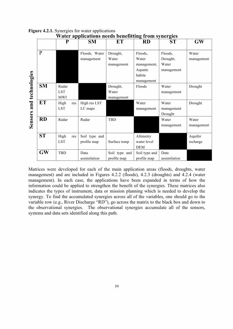
59
Figure 4.2.1. Synergies for water applications Water applications needs benefitting from synergies
Sens
ors a
nd te
chno
logi
es
P SM ET RD ST GW
P Floods, Water management
Drought, Water management
Floods, Water management, Aquatic habita management
Floods, Drought, Water management
Water management
SM Radar LST MWI
Drought, Water management
Floods Water management
Drought
ET High res LST
High res LST LC maps
Water management
Water management Drought
Drought
RD Radar Radar TBD Water management
Water management
ST High res LST
Soil type and profile map
Surface temp
Altimetry water level DEM
Aquifer recharge
GW TBD Data assimilation
Soil type and profile map
Soil type and profile map
Data assimilation
Matrices were developed for each of the main application areas (floods, droughts, water management) and are included in Figures 4.2.2 (floods), 4.2.3 (droughts) and 4.2.4 (water management). In each case, the applications have been expanded in terms of how the information could be applied to strengthen the benefit of the synergies. These matrices also indicates the types of instrument, data or mission planning which is needed to develop the synergy. To find the accumulated synergies across all of the variables, one should go to the variable row (e.g., River Discharge “RD”), go across the matrix to the black box and down to the observational synergies. The observational synergies accumulate all of the sensors, systems and data sets identified along this path.

60
Figure 4.2.2 shows that observations of all of the EWVs contributes to flood prediction and response. Data from satellites play a critical role for informing flood prediction systems, assessing the vulnerability of the environment to heavy rain events (e.g., the degree to which soil is saturated and reservoirs are filled or to ice jamming events), and monitoring flood extent and damage. The data requirements for this application are quite demanding since high-frequency, high-spatial resolution and low latency data are most effective. Figure 4.2.2. Synergies for flood prediction and recovery applications
User needs benefitting from synergies
Sens
ors a
nd te
chno
logi
es’ s
yner
gies
P SM ET RD ST GW
P Flood warning
Water balance Flood warning Dam operations
Dam operations
Recharge
SM Radar LST MWI
Vegetation growth Water balance
Flood impact Run-off prediction
Leakage Drought
Drought monitoring
ET High res LST
High res LST LC Maps
Water loss Storage water loss
Drought monitoring
RD Radar Radar TBD Storage drainage and refill Food predict
Recharge/ discharge
ST High res LST
Soil Type and profile map
Surface temp
Altimetry water level DEM
Aquifer recharge
GW TBD Data assimilation
Soil type and profile map
Soil type and profile map
Data assimilation
Observation synergies
Radar, LST, MWI
Radar, LST, LC maps, Soil maps, Data assimilation.
LST, LC maps, Surface Temp., soil maps
Radar, Altimetry, Water levels, soil maps
LST, Soil maps, Altimetry, Data assimilation
Data assimilation

61
Figure 4.2.3 shows the data needed to monitor droughts. As drought represents a more slowly evolving phenomenon, arising from the absence of rainfall, the requirements for frequent observations tends to be lower, although the spatial resolution requirements are still generally high in order to properly assess local impacts of drought. The focus for drought applications lies in monitoring its development and measuring its various impacts including its effects on vegetation and crops, ecosystems and surface and subsurface water storage and flows. The latency for real-time drought and its effects is also significant because short-term decisions are often needed to mitigate drought’s impacts. Figure 4.2.3. Synergies for drought monitoring and drought response
User needs benefitting from synergies
Sens
ors a
nd te
chno
logi
es’ s
yner
gies
P SM ET RD ST GW
P Irrigation scheduling Drought monitor
Water balance Monitor low flows (drought)
Water avail Drought monitor and recharge
SM Radar LST MWI
Vegetation growth
Streamflow prediction
Leakage from reservoir Drought
Drought monitoring
ET High res LST High res LST LC Maps
TBD Storage water loss
Drought monitoring
RD Radar Radar TBD Storage drainage and refill
Recharge/ discharge
ST Radar
Soil Type and profile map
Surface temp
Altimetry water level DEM
Aquifer recharge
GW TBD Data assimilation
Soil type and profile map
Soil type and profile map
TBD
Observation synergies
Radar, LST, MWI, LST
LST, MWI, LC map, Radar, Soil type and profile map, Data assimilation
LST, LC map, Surface temp. Soil type and profile map
Radar, Altimetry, Soil map
Altimetry Soil Map Data assimilation Surface temp.
Data assimilation

62
Figure 4.2.4 identifies the specific applications of data for water resource management. It should be noted that often floods and droughts are included in a nation’s water resource management activity and the information must therefore be fully integrated for proper service delivery. The water management function involves the allocation of water for industrial, agricultural and domestic use and the allocation or preservation of water for ecosystems and for meeting the requirements of negotiated agreement; monitoring day-to-day water availability to ensure those requirements can be met; and developing longer-range plans for water to meet future development needs. Although we have not addressed the issue here, water pollution and treatment is part of water management. Models are used extensively and it is important to ensure that water managers have access to the inputs needed to allow those models to produce timely outputs for reliable decision making. Water management relies on systematic observations that deliver observations over the full range of water variables. Depending on the level at which this management take place (national, state or provincial, or local) the requirements for spatial resolution may vary. Figure 4.2.4. Synergies for water resource management
User needs benefitting from synergies
Sens
ors a
nd te
chno
logi
es’ s
yner
gies
P SM ET RD ST GW
P Irrigation water allocation and scheduling
Water balance Irrigation water allocation and scheduling
Water allocation and treatment
Water allocation Dam operation
Water Recharge
SM Radar LST MWI
Vegetation growth
Discharge predict for allocation
Leakage from reservoirs
Aquifer water availability
ET High res LST High res LST LC Maps
TBD Storage water loss
Aquifer water availability
RD Radar Radar TBD Storage change and refill strategy
In mountains, GW discharge
ST Radar Soil Type and profile map
Surface temp Altimetry water level DEM
Aquifer recharge
GW TBD Data assimilation
Soil type and profile map
Soil type and profile map
Data assimilation
Observation synergies
Radar, High res LST, MWI
High res LST, LC Maps, Radar, Soil maps, Data assimilation
Surface temp/LST, LC maps, Soil maps,
Radar, Altimetry Soil type and profile map
Radar, soil maps, Surface temp. Data assimilation Altimetry
Data assimilation, soil maps

63
5. Recommendations regarding the Water Constellations The FS indicated that proper planning and coordination of a water cycle constellation could be constructed with existing and planned components of priority water cycle variable observations, considering synergies among them. Sensor requirements for observing water variables considering synergies of other variable observations are shown in Table 5.1. Table 5.1 Components of a Water Constellation The following recommendations for the Water Constellation can be made: The MWI constellation is a key component of the water cycle constellation, providing precipitation, soil moisture and evapotranspiration monitoring. It can also monitor SST under all-weather conditions, including snow and ice. Without immediate action, the impending loss of DMSP/SSMI and GCOM-W/AMSR-2 capabilities will lead to significant degradation of the precipitation observation.
l Consideration should be given to MWI missions to follow-on after DMSP-19/SSMI in the early morning orbit and GCOM-W/AMSR-2.
l Efforts should be strengthen to coordinate with China and Russia to provide their FY and METEOR series MWI and MWS data for use in estimating precipitation.
l Follow-on L-band MWI / radar soil moisture missions to follow SMOS and SMAPshould be studied as a part of the MWI constellation.
l The use of a larger antenna MWI to fill spatial resolution gaps for soil moisture, SST, and snow/ice extent monitoring should be studied.
A precipitation radar is important to calibrate precipitation estimates derived from a MWI constellation, because only this can provide the three-dimensional structure of a precipitation system. Precipitation radar data is also used for global rainfall maps (eg GSMaP), which are used for weather and hydrological applications. Next-generation precipitation radars with much higher sensitivity and wider scan should be developed to ensure continuity of the
Instrument
Variable

64
critical precipitation data. Synergistic observations of GPM and EarthCARE should be promoted to provide complete picture of the process and chracteristics of aerosols, cloud and precipitation. Coordination of existing and future virtual constellation of TIR, optical and L-, C-, and X-band radars, altimeter and gravity missions should be improved to maximize the contributions to observations. Satellite mission coordination should include data aquisition and product generation. The potential to improve the revisit time of altimeter missions by combining existing and future missions for monitoring river discharge and surface water storage should be studied. GRACE-type missions should be continued for groundwater monitoring. Data assimilation systems should be developed to use actual data in a more optimal way. A broad water constellation that incorporates data assimilation has the potential to more effectively exploit existing and planned assets. 6. Way forward This Water Constellation Feasibility Study addresses the observation requirements, capabilities, gaps and synergies for six high-priority water parameters. The FS shows that their requirements are partially met at present and that their observation capabilities need to be improved in temporal and spatial resolution and that dissemination needs to be improved through decreased data latency. Observation continuity is also in question, in particular, MWI data continuity. There are many potential synergies among precipitation, soil moisture and evapotranspiration observations that could lead to a better characterization of the global water cycle. Close coordination among those existing and future observation systems is very desirable and useful. Observations of river discharge and surface water storage can utilize the same observation systems used by innovative altimeter missions for water level and existing and future optical and radar constellations for water extent. Groundwater monitoring, which cannot be measured with conventional optical and radar-based remote sensing techniques, has progressed the most in last decade. Data assimilation plays a key role in combining those observations of parameters and models. Data assimilation models and methodologies must continue to evolve to adapt to the new changing data requirements and opportunities. Snow and ice were not addressed in the study, except for some references to user needs in the section on surface water storage (Section 3.5). Snow and ice are very important elements of the water cycle and need to be considered as a priority parameter in future studies . This Feasibility Study responds to the GEOSS Water Strategy Recommendation C1 and the

65
CEOS priority to try to more effectively capture fluxes and storage of water quantities. One of the remaining CEOS actions is C10 which requires a water colour feasibility study and the assessment of hyperspectral technologies. While C1 and C10 feasibility studies are conducted rather independently, the results may be integrated in the next phase. It is recommended that CEOS maintain some form or a water activity or advisory group to ensure that the benefits of these studies are incorporated into future CEOS discussions and plans.
66
7. References Allen, R., W. Bastiaanssen, A. Kilic, (2015): “Additional ET observation platforms: Towards and integrated
observation capability.” International Workshop on Evapotranspiration Mapping for Water Security, Sep. 15-17, Washington, DC.
Anderson, M. C., J. Norman, G. Diak, W. Kustas, and J. R. Mecikalski, (1997): “A two-source time-integrated model for estimating surface energy fluxes using thermal infrared remote sensing.” Remote Sens. Environ., 60: 195-216.
Anderson, M. C., W. Kustas, J. M. Norman, C. R. Hain, J. R. Mecikalski, L. Schultz, M. P. González- Dugo, C. Cammalleri, G. d'Urso, A. Pimstein, and F. Gao, (2011): “Mapping daily evapotranspiration at field to continental scales using geostationary and polar orbiting satellite imagery.” Hydrol. Earth Syst. Sci., 15: 223-39. doi: 10.5194/hess-15-223-2011.
Asian Disaster Reduction Center, (2014): “Natural Diaster Data Book 2014 An Analytical Overview” http://www.adrc.asia/publications/databook/DB2014_e.html
CEOS, (2016): The CEOS Database. Available at: http://database.eohandbook.com/. CEOS, (2016): The Earth Observation Handbook. Available at: http://www.eohandbook.com/. Committee on Earth Science and Applications from Space: A Community Assessment and Strategy for the
Gure, National Research Council, (2007): “Earth Science and Applications from Space: National Imperatives for the Next Decade and Beyond”, http://nap.edu/11820
Chambon, P., R. Roca, I. Jobard, and M. Capderou, (2012): “The sensitivity of tropical rainfall estimation from satellite to the configuration of the microwave imager constellation.” IEEE Geoscience and Remote Sensing Letters, 10 (5): 996-1000. doi: 10.1109/LGRS.2012.2227668.
Friedl, L., and S. Unninayar, (2010): GEO Task US-09-01a: Critical Earth Observations Priorities, Water Societal Benefit Area. GEO Unser Interface Committee.
Hain, C. R., J. R. Mecikalski, and M. C. Anderson, (2009): “Retrieval of an available water-based soil moisture proxy from thermal infrared remote sensing. Part I: Methodology and validation.” J. Hydrometeor., 10: 665-83.
Hain, C. R., W. T. Crow, J. R. Mecikalski, M. C. Anderson, and T. Holmes, (2011): “An intercomparison of available soil moisture estimates from thermal infrared and passive microwave remote sensing and land surface modeling.” J. Geophys. Res., 116: D15107. doi: 10.1029/2011JD015633.
Hain, C. R., W. T. Crow, M. C. Anderson, and M. T. Yilmaz, (2015): “Diagnosing neglected soil moisture source/sink processes via a thermal infrared-based two-source energy balance model.” J. of Hydrometeor., 16: 1070-86.
Holmes, T. R., C. R. Hain, M. C. Anderson, and W. T. Crow, (2016): "Cloud tolerance of remote-sensing technologies to measure land surface temperature." Hydrology and Earth System Sciences, 20 (8): 3263-75. doi: 10.5194/hess-20-3263-2016.
Hou, A. Y., R. K. Kakar, S. Neeck, A. A. Azarbarzin, C. D. Kummerow, M. Kojima, R. Oki, K. Nakamura, and T. Iguchi, (2014): The Global Precipitation Measurement Mission. Bull. Amer. Meteor. Soc., 95, 701–722, doi:10.1175/BAMS-D-13-00164.1
Huffman, G.J., S.T. Brown, V. Chandrasekar, G. Skofronick-Jackson, C. Kidd, E. Kim, W. Meier, J. Piepmeier, P. Sellers, F. Joseph Turk, N.-Y. Wang, 2016: Multidisciplinary Earth System Science: An Approach to Enhance Value from Passive Microwave Earth Observing Satellite Sensors. White Paper submitted for RFI #2 in the NASEM Decadal Survey for Earth Sci. and Appl. from Space, 12 pp. http://surveygizmoresponseuploads.s3.amazonaws.com/fileuploads/15647/2604456/107-083e64649aa44dbf093c93fbaa67ba30_HuffmanGeorgeJMicrowaveConst.pdf
67
Huffman, G.J., V. Chandrasekar, G. De Amici, G. Skofronick-Jackson, C. Kidd, W. Meier, J. Piepmeier, F. Joseph Turk, 2016: Global Precipitation Observations to Advance Water/Energy Cycle, Climate, Model, and Disaster Science. White Paper submitted for RFI #2 in the NASEM Decadal Survey for Earth Sci. and Appl. from Space, 13 pp. http://surveygizmoresponseuploads.s3.amazonaws.com/fileuploads/15647/2604456/191-99875a374c06b8bd3ecdd7741de551b9_HuffmanGeorgeJPrecipConst.pdf
JAXA, and GPM, (2016): Report on Post-GPM Study WG. GPM Utilization Study Committee. Jones, J.W., (2015): Efficient wetland surface water detection and monitoring via Landsat: Comparison
with in situ data from the Everglades Depth Estimation Network. Remote Sensing. Vol 7, issue 9, 12503-12538.
Kim, J-W, Z. Lu, J.W. Jones, C.K. Shum, H. Lee and Y. Jia, (2014): Monitoring Everglades’s freshwater marsh water level using L-band synthetic aperture radar backscatter. Remote Sensing of Environment. B. 150 p. 66-81
Liu, Y. Y., R. M. Parinussa, W. A. Dorigo, R. A. M. De Jeu, W. Wagner, A. I. J. M. van Dijk, M. F. McCabe, and J. P. Evans, (2011): “Developing an improved soil moisture dataset by blending passive and active microwave satellite-based retrievals.” Hydol. Earth Syst. Sci., 15: 425-36.
Merzouki, A., and H. McNairn, (2015): “A hybid (multi-angle and multipolarization) approach to soil moisture retrieval using the integral equation model: Preparing for the RADASAT constellation mission.” Canadian Journal of Remote Sensing, 41 (5): 349-62.
Reed, P. M., N. W. Chaney, J. D. Herman, M. P. Ferringer, and E. F. Wood, (2015): “Internationally coordinated multi-mission planning is now critical to sustain the space-based rainfall observations needed for managing floods globally.” Eniron. Res. Lett., 10: 024010.
Seneviratne, S. I., T. Corti, E. L. Davin, M. Hirschi, E. B. Jaeger, I. Lehner, B. Orlowsky, and A. J. Teuling, (2010): “Investigating soil moisture-climate interactions in a changing climate: A review.” Earth-Science Reviews, 99: 3-4, 125-61. doi: 10.1016/j.earscirev.2010.02.004.
Stocker, E. F., and K. Furukawa, (2011): “CEOS Precipitation Constellation (PC) White Paper #1: Availability of microwaver imagers in the post-Global Precipitation Measurement (GPM) era.” CEOS.
Viger, Roland, L. Hay, J. Jones and G. Buell, (2011): Parameterization of spatially distributed, physically based hydrologic models for ecological flow requirement modeling. USGS SIR. 120 pp.
Vinukollu, R. K., E. F. Wood, G. R. Ferguson, and J. B. Fisher, (2011): “Global estimates of evapotranspiration for climate studies using multi-sensor remote sensing data: Evaluation of three process-based approaches.” Remote Sensing of Environment, 115: 801-23.
Walker, J. P., and P. R. Houser, (2004): “Requirements of a global near-surface soil moisture satellite mission: accuracy, repeat time, and spatial resolution.” Advances in Water Resources, 27: 785-801.
Yamaji, M., (2016): CEOS Water Constellation Feasibility Study: Preliminary Sampling Analysis. JAXA/EORC.

68
Appendix A Relevant CEOS missions B GCOS/ECV C WMO-SOG D List of Acronyms Appendix A: Relevant CEOS missions 1. Precipitation observations Table A. 1.1. Microwave Imagers Satellite Organiz
ation Launch (Target)
Mission Life
LST Instrument
Technical characteristics
DMSP F-16
ditto Oct 2003 Oct 2016 LST: 21:32 SSM/IS Waveband: Microwave: 19 - 183 GHz (24 frequencies) Spatial resolution: 25 x 17 km to 70 x 42 km Swath width: 1700 km Accuracy: Data Access: Data Format:
DMSP F-17
ditto Nov 2006 Dec 2015 Altitude: 850 km Period: 101 mins Inclination: 98.7 degree LST: 17:31 Asc./desc.: Ascending
SSM/IS ditto
DMSP F-18
ditto Oct 2009 Dec 2015 Altitude: 850 km Period: 101 mins Inclination: 98.7 degree LST: 17:31 Asc/desc: Ascending
SSM/IS ditto
GCOM-W1
JAXA May 2012 May 2017 Altitude: 700 km Period: 98 mins Inclination: 98.2 degree LST: 13:30 Asc/desc: Ascending
AMSR2
Waveband: 6.925 GHz, 7.3 GHz, 10.65 GHz, 18.7 GHz, 23.8 GHz, 36.5 GHz, 89.0 GHz Spatial resolution: 5 - 50 km Swath width: 1450 km Accuracy: Sea surface temperature: 0.5 K, Sea ice cover: 10%, Cloud liquid water: 0.05 kg/m2, Precipitation rate: 10%, Water vapour: 3.5 kg/m2 through total column, Sea surface wind

69
Satellite Organization
Launch (Target)
Mission Life
LST Instrument
Technical characteristics
speed 1.5 m/s Data Access: Open Access Data Format: HDF5
FY-3A CMA/NRSCC
May 2008 Dec 2016 Altitude: 830 km Period: 101 mins Inclination: 98.753 degree Repeat cycle: LST: 10:10 Asc/desc: Descending
MWRI Waveband: 12 channels, 6 frequencies: 10.65 GHz, 18.7 GHz, 23.8 GHz, 36.5 GHz, 89 GHz, 150 GHz Spatial resolution: 7.5 x 12 km at 150 GHz to 51 x 85 km at 10.65 GHz Swath width: 1400 km Accuracy: Data Access: Constrained Access
FY-3B ditto Nov. 2010 Dec. 2016 LST: 14:00 Asc/desc: Ascending
MWRI ditto
FY-3C ditto Sep. 2013 Sep. 2016 LST: 10:00 Asc/desc: Descending
MWRI ditto
FY-3D ditto Dec. 2016 Dec. 2018 LST: 14:00 Asc/desc: Ascending
MWRI ditto
FY-3F ditto 2019 2022 LST: 14:00 Asc/desc: Ascending
MWRI ditto
FY-3RM NSMC-CMA
2020 2025 N/A MWRI, PR
ditto
GPM NASA/JAXA
Feb. 2014 May 2017 non-sun-synchronous Altitude: 407 km Period: 95 mins Inclination: 65 degree Asc/desc: TBD
GMI Waveband: 10.65 GHz, 18.7 GHz, 23.8 GHz, 36.5 GHz, 89.0 GHz, 165.5 GHz, 183.31 ± 3 GHz, 183.31 ± 8 GHz Spatial resolution: Horizontal: 36 km cross-track at 10.65 GHz (required Swath width: 800 km Accuracy: 0.65 - 1.5 K Data Access: Open Access Data Format: HDF-EOS(HDF5)
METEOR-M-N2
ROSHYDROMET/ROSCOSMOS
July 2014 5 years Sun-synchronous altitude of ~ 825 km, inclination = 98.8º, period = 101.41 minutes, LTAN (Local Time on Ascending Node) at 9:30 hours.
MTVZA-GY
10.6-183.3 (26 channels) 89 x 189 km – 9 -21 km 1500 km

70
Satellite Organization
Launch (Target)
Mission Life
LST Instrument
Technical characteristics
METEOR-M-N2-1
ditto 2015 5 years Afternoon orbit? ditto ditto
METOP-SG-B
EUMETSAT/CNES/ESA
2022 2030 817 km MWI 18 channels (eight dual-polarised) in the frequency range from 18.7 to 183 GHz, at a spatial resolution from 10 km to 50 km
Table A.1.2. Microwave Sounder. Satellite Organiz
ation Launch (Target)
Mission Life
LST Instrument
Technical characteristics
NOAA-18 NOAA May 2005 Dec. 2015 Altitude: 870 km Period: 102.1 mins Inclination: 98.75 degree Repeat cycle: LST: 14:00 Asc/desc: Ascending
AMSU-A
Waveband: 15 channels, 23.8 - 89.0 GHz Spatial resolution: 48 km Swath width: 2054 km Accuracy: Temperature profile: 2 K, humidity: 3 kg/m2, ice & snow cover: 10% Data Access: Open Access
NOAA-19 NOAA Feb. 2009 Dec. 2015 Altitude: 870 km Period: 102.1 mins Inclination: 98.75 degree Repeat cycle: LST: 14:00 Asc/desc: Ascending
MHS Waveband: 89 GHz, 166 GHz and 3 channels near 183 GHz Spatial resolution: Vertical: 3 - 7 km, Horizontal: 30 - 50 km Swath width: 1650 km Accuracy: Cloud water profile: 10 g/m2, specific humidity profile: 10 - 20% Data Access: Open Access
NPP NASA/NOAA
Oct. 2011 Sep. 2020 Altitude: 824 km Period: 101 mins Inclination: 98.7 degree Repeat cycle: 16 days LST: 13:30 Asc/desc: Ascending
ATMS Waveband: 22 bands, 23-184 GHz Spatial resolution: 5.2 - 1.1 degree Swath width: 2300 km Accuracy: 0.75 K - 3.60 K Data Access: Open Access
Megha-Tropiques
CNES/ISRO
Oct. 2011 Dec. 2016 Non-sun-synchronous Altitude: 867 km Period: 102.16 mins Inclination: 20 degree Asc/desc: Ascending
SAPHIR
Waveband: 183.3 GHz (6 channels) Spatial resolution: 10 km Swath width: 2200 km Accuracy: Data Access: Constrained Access
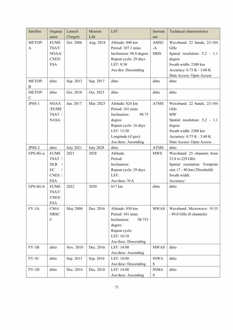
71
Satellite Organization
Launch (Target)
Mission Life
LST Instrument
Technical characteristics
METOP-A
EUMETSAT/NOAA/CNES/ESA
Oct. 2006 Aug. 2018 Altitude: 840 km Period: 107.1 mins Inclination: 98.8 degree Repeat cycle: 29 days LST: 9:30 Asc/des: Descending
AMSU-A MHS
Waveband: 22 bands, 23-184 GHz Spatial resolution: 5.2 - 1.1 degree Swath width: 2300 km Accuracy: 0.75 K - 3.60 K Data Access: Open Access
METOP-B
ditto Sep. 2012 Sep. 2017 ditto ditto ditto
METOP-C
ditto Oct. 2018 Oct. 2023 ditto ditto ditto
JPSS-1 NOAA /EUMETSAT / NASA
Jan. 2017 Mar. 2023 Altitude: 824 km Period: 101 mins Inclination: 98.75 degree Repeat cycle: 16 days LST: 13:30 Longitude (if geo): Asc/desc: Ascending
ATMS Waveband: 22 bands, 23-184 GHz MW Spatial resolution: 5.2 - 1.1 degree Swath width: 2300 km Accuracy: 0.75 K - 3.60 K Data Access: Open Access
JPSS-2 ditto July 2021 July 2028 ditto ATMS ditto EPS-SG-a EUME
TSAT / DLR / EC / CNES / ESA
2021 2028 Altitude: Period: Inclination: Repeat cycle: 29 days LST: Asc/desc: N/A
MWS Waveband: 25 channels from 23.8 to 229 GHz Spatial resolution: Footprint size 17 - 80 km (Threshold) Swath width: Accuracy:
EPS-SG-b EUMETSAT/CNES/ESA
2022 2030 817 km ditto ditto
FY-3A CMA/NRSCC
May 2008 Dec. 2016 Altitude: 830 km Period: 101 mins Inclination: 98.753 degree Repeat cycle: LST: 10:10 Asc/desc: Descending
MWAS Waveband: Microwave: 19.35 - 89.0 GHz (8 channels)
FY-3B ditto Nov. 2010 Dec. 2016 LST: 14:00 Asc/desc: Ascending
MWAS ditto
FY-3C ditto Sep. 2013 Sep. 2016 LST: 10:00 Asc/desc: Descending
INWAS
ditto
FY-3D ditto Dec. 2016 Dec. 2018 LST: 14:00 Asc/desc: Ascending
INMAS
ditto
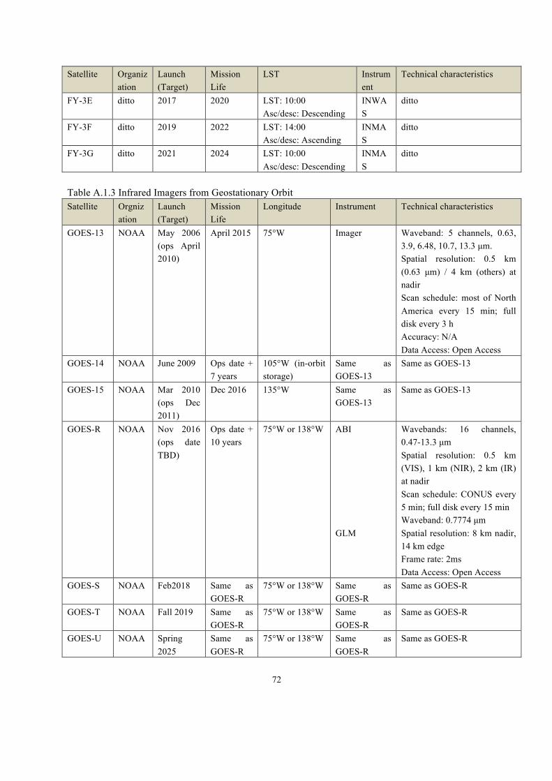
72
Satellite Organization
Launch (Target)
Mission Life
LST Instrument
Technical characteristics
FY-3E ditto 2017 2020 LST: 10:00 Asc/desc: Descending
INWAS
ditto
FY-3F ditto 2019 2022 LST: 14:00 Asc/desc: Ascending
INMAS
ditto
FY-3G ditto 2021 2024 LST: 10:00 Asc/desc: Descending
INMAS
ditto
Table A.1.3 Infrared Imagers from Geostationary Orbit Satellite Orgniz
ation Launch (Target)
Mission Life
Longitude Instrument Technical characteristics
GOES-13 NOAA May 2006 (ops April 2010)
April 2015 75°W Imager Waveband: 5 channels, 0.63, 3.9, 6.48, 10.7, 13.3 µm. Spatial resolution: 0.5 km (0.63 µm) / 4 km (others) at nadir Scan schedule: most of North America every 15 min; full disk every 3 h Accuracy: N/A Data Access: Open Access
GOES-14 NOAA June 2009 Ops date + 7 years
105°W (in-orbit storage)
Same as GOES-13
Same as GOES-13
GOES-15 NOAA Mar 2010 (ops Dec 2011)
Dec 2016 135°W Same as GOES-13
Same as GOES-13
GOES-R NOAA Nov 2016 (ops date TBD)
Ops date + 10 years
75°W or 138°W ABI GLM
Wavebands: 16 channels, 0.47-13.3 µm Spatial resolution: 0.5 km (VIS), 1 km (NIR), 2 km (IR) at nadir Scan schedule: CONUS every 5 min; full disk every 15 min Waveband: 0.7774 µm Spatial resolution: 8 km nadir, 14 km edge Frame rate: 2ms Data Access: Open Access
GOES-S NOAA Feb2018 Same as GOES-R
75°W or 138°W Same as GOES-R
Same as GOES-R
GOES-T NOAA Fall 2019 Same as GOES-R
75°W or 138°W Same as GOES-R
Same as GOES-R
GOES-U NOAA Spring 2025
Same as GOES-R
75°W or 138°W Same as GOES-R
Same as GOES-R

73
Satellite Orgnization
Launch (Target)
Mission Life
Longitude Instrument Technical characteristics
METEOSAT-7
EUMETSAT
Sep 1997 (ops until 2006; providing INDOEX coverage since then)
Ops date + 5 years
0°W (until Dec 2006); 57.5ºE (present)
MVRI Wavebands: 3 channels (0.72, 6.4, 11.5 µm) Spatial resolution: 2.5 km (VIS), 5 km (others) at nadir Scan schedule: full disk every 30 min Data Access: Open Access
METEOSAT-8
EUMETSAT
Aug 2002 (ops ended in Apr 2008 but moved to 41.5°E to replace METEOSAT-7)
Ops date + 7 years
41.5°E SEVIRI Wavebands: 12 channels, 0.6-13.4 µm Spatial resolution: 1 km (VIS), 3 km (others) at nadir Scan schedule: full disk every 15 min Data Access: Open Access
METEOSAT-9
EUMETSAT
Dec 2005 (ops Apr 2007)
Same as METEOSAT-8
9.5°E Same as METEOSAT-8
Same as METEOSAT-8, except used for Rapid Scan Service only
METEOSAT-10
EUMETSAT
July 2012 (ops Jan 2013)
Same as METEOSAT-8
0°W Same as METEOSAT-8
Same as METEOSAT-8
METEOSAT-11
EUMETSAT
July 2015 (in storage until 2018)
Same as METEOSAT-8
In-orbit storage at 3.4 °W
Same as METEOSAT-8
Same as METEOSAT-8
MTG-I1 EUMETSAT
2020 Ops date + 8 years
9.5°E FCI LI
Wavebands: 16 channels, 0.444-13.3 µm Spatial resolution: 1 km (VIS), 2 km (others) at nadir Scan schedule: full disk every 10 min Waveband: 0.7774 µm Spatial resolution: 8 km nadir, 14 km edge Frame rate: 2ms Data Access: Open Access
MTG-I2 EUMETSAT
2023 Same as MTG-I2
Same as MTG-I2
Same as MTG-I2
Same as MTG-I2
MTG-I3 EUMETSAT
2026 Same as MTG-I2
Same as MTG-I2
Same as MTG-I2
Same as MTG-I2
MTG-I4 EUMETSAT
2031 Same as MTG-I2
Same as MTG-I2
Same as MTG-I2
Same as MTG-I2

74
Satellite Orgnization
Launch (Target)
Mission Life
Longitude Instrument Technical characteristics
Himawari-8
JAXA Oct 2014 (ops Jul 2015)
Ops date + 8 years
140.7°E AHI Wavebands: 16 channels, 0.47-13.3 µm Spatial resolution: 0.5 km (VIS), 1 km (NIR), 2 km (IR) at nadir Scan schedule: full disk every 10 min Data Access: Constrained Access (limited by bandwidth; third-party re-distribution permitted)
Himawari-9
JAXA Late 2016 / early 2017
Same as Himawari-8
Same as Himawari-8
Same as Himawari-8
Same as Himawari-8
Kalpana-1 ISRO Sep 2002 2016? 74.0°E VHRR Wavebands: 3 channels, 0.65, 6.40, 11.5 µm Spatial resolution: 2 km (VIS), 8 km (WV & IR) at nadir Scan schedule: full disk every hour
INSAT-3D
ISRO Jul 2013 7.7 years 82.0°E VHRR/2 Wavebands: 6 channels, 0.65-12.0 µm Spatial resolution: 1 km (VIS), 8 km (WV), 4 km (others) at nadir Scan schedule: full disk every 30 min
INSAT-3DR
ISRO Aug 2016 Same as INSAT-3D
Same as INSAT-3D
Same as INSAT-3D
Same as INSAT-3D
INSAT-3DS
ISRO 2022 Same as INSAT-3D
Same as INSAT-3D
Same as INSAT-3D
Same as INSAT-3D
COMS-1 KARI Jun 2010 2019 128.2°E MI Wavebands: 5 channels, 0.65-12.0 µm Spatial resolution: 1 km (VIS), 4 km (others) at nadir Scan schedule: full disk every 30 min
GEO-KOMPSAT-2A
KARI 2018 10 years Same as COMS-1
AMI Wavebands: 16 channels, 0.455-13.3 µm Spatial resolution: 0.5 km (0.642 µm), 1 km (other VIS), 2 km (IR) at nadir Scan schedule: full disk every
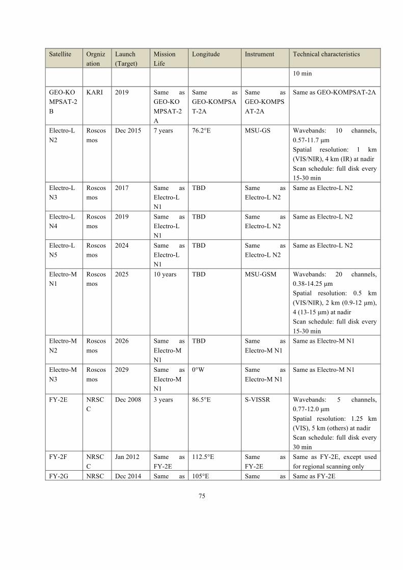
75
Satellite Orgnization
Launch (Target)
Mission Life
Longitude Instrument Technical characteristics
10 min
GEO-KOMPSAT-2B
KARI 2019 Same as GEO-KOMPSAT-2A
Same as GEO-KOMPSAT-2A
Same as GEO-KOMPSAT-2A
Same as GEO-KOMPSAT-2A
Electro-L N2
Roscosmos
Dec 2015 7 years 76.2°E MSU-GS Wavebands: 10 channels, 0.57-11.7 µm Spatial resolution: 1 km (VIS/NIR), 4 km (IR) at nadir Scan schedule: full disk every 15-30 min
Electro-L N3
Roscosmos
2017 Same as Electro-L N1
TBD Same as Electro-L N2
Same as Electro-L N2
Electro-L N4
Roscosmos
2019 Same as Electro-L N1
TBD Same as Electro-L N2
Same as Electro-L N2
Electro-L N5
Roscosmos
2024 Same as Electro-L N1
TBD Same as Electro-L N2
Same as Electro-L N2
Electro-M N1
Roscosmos
2025 10 years TBD MSU-GSM Wavebands: 20 channels, 0.38-14.25 µm Spatial resolution: 0.5 km (VIS/NIR), 2 km (0.9-12 µm), 4 (13-15 µm) at nadir Scan schedule: full disk every 15-30 min
Electro-M N2
Roscosmos
2026 Same as Electro-M N1
TBD Same as Electro-M N1
Same as Electro-M N1
Electro-M N3
Roscosmos
2029 Same as Electro-M N1
0°W Same as Electro-M N1
Same as Electro-M N1
FY-2E NRSCC
Dec 2008 3 years 86.5°E S-VISSR Wavebands: 5 channels, 0.77-12.0 µm Spatial resolution: 1.25 km (VIS), 5 km (others) at nadir Scan schedule: full disk every 30 min
FY-2F NRSCC
Jan 2012 Same as FY-2E
112.5°E Same as FY-2E
Same as FY-2E, except used for regional scanning only
FY-2G NRSC Dec 2014 Same as 105°E Same as Same as FY-2E
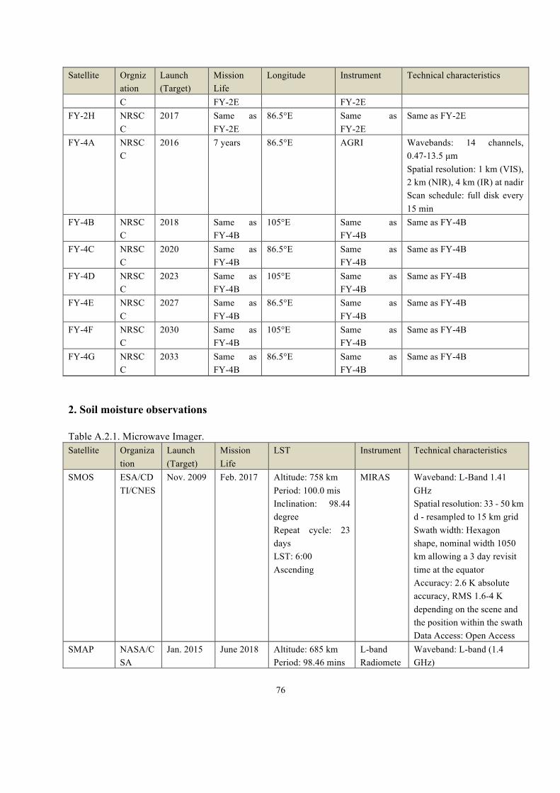
76
Satellite Orgnization
Launch (Target)
Mission Life
Longitude Instrument Technical characteristics
C FY-2E FY-2E FY-2H NRSC
C 2017 Same as
FY-2E 86.5°E Same as
FY-2E Same as FY-2E
FY-4A NRSCC
2016 7 years 86.5°E AGRI Wavebands: 14 channels, 0.47-13.5 µm Spatial resolution: 1 km (VIS), 2 km (NIR), 4 km (IR) at nadir Scan schedule: full disk every 15 min
FY-4B NRSCC
2018 Same as FY-4B
105°E Same as FY-4B
Same as FY-4B
FY-4C NRSCC
2020 Same as FY-4B
86.5°E Same as FY-4B
Same as FY-4B
FY-4D NRSCC
2023 Same as FY-4B
105°E Same as FY-4B
Same as FY-4B
FY-4E NRSCC
2027 Same as FY-4B
86.5°E Same as FY-4B
Same as FY-4B
FY-4F NRSCC
2030 Same as FY-4B
105°E Same as FY-4B
Same as FY-4B
FY-4G NRSCC
2033 Same as FY-4B
86.5°E Same as FY-4B
Same as FY-4B
2. Soil moisture observations Table A.2.1. Microwave Imager. Satellite Organiza
tion Launch (Target)
Mission Life
LST Instrument Technical characteristics
SMOS ESA/CDTI/CNES
Nov. 2009 Feb. 2017 Altitude: 758 km Period: 100.0 mis Inclination: 98.44 degree Repeat cycle: 23 days LST: 6:00 Ascending
MIRAS Waveband: L-Band 1.41 GHz Spatial resolution: 33 - 50 km d - resampled to 15 km grid Swath width: Hexagon shape, nominal width 1050 km allowing a 3 day revisit time at the equator Accuracy: 2.6 K absolute accuracy, RMS 1.6-4 K depending on the scene and the position within the swath Data Access: Open Access
SMAP NASA/CSA
Jan. 2015 June 2018 Altitude: 685 km Period: 98.46 mins
L-band Radiomete
Waveband: L-band (1.4 GHz)

77
Satellite Organization
Launch (Target)
Mission Life
LST Instrument Technical characteristics
Inclination: 98.12 degree Repeat cycle: LST: 18:00 Ascending
r L-band Radar
Spatial resolution: 40 km spatial resolution; 3 days temporal resolution Swath width: 1000 km swath Accuracy: 1.3 K accuracy brightness temperature Data Access: Open Access
GCOM-W1
JAXA May 2012 May 2017 Altitude: 700 km Period: 98 mins Inclination: 98.2 degree LST: 13:30 Asc/desc: Ascending
AMSR2 Waveband: 6.925 GHz, 7.3 GHz, 10.65 GHz, 18.7 GHz, 23.8 GHz, 36.5 GHz, 89.0 GHz Spatial resolution: 5 - 50 km Swath width: 1450 km Data Access: Open Access
GPM NASA/JAXA
Feb 2014 May 2017 non-sun-synchronous Altitude: 407 km Period: 95 mins Inclination: 65 degree Asc/desc: TBD
GMI Waveband: 10.65 GHz, 18.7 GHz, 23.8 GHz, 36.5 GHz, 89.0 GHz, 165.5 GHz, 183.31 ± 3 GHz, 183.31 ± 8 GHz Spatial resolution: Horizontal: 32 km x 19 km at 10.65 GHz Swath width: 885 km Accuracy: 0.65 - 1.5 K Data Access: Open Access Data Format: HDF-EOS(HDF5)
Table A.2.2. Microwave radar Satellite Organiza
tion Launch (Target)
Mission Life
LST Instrument Technical characteristics
Radarsat-2 CSA/MDA
Dec. 2007 Apr. 2019 Altitude: 798 km Period: 100.7 mins Inclination: 98.6 degree Repeat cycle: 24 days LST: 18:00 Ascending
SAR Waveband: C band 5.405 GHz. Spatial resolution: Standard: 27 - 17 x 25 m; Wide: 40 - 19 x 25 m; Fine: 10 - 7 x 8 m; ScanSAR (N/W): 80 - 38 x 60 m / 160 - 172 x 100 m, Extended (H/L): 18 - 16 x 25 m / 60 - 23 x 25 m (4 looks); Ultra-Fine: 4.6 - 2.1 x 2.8 m

78
Satellite Organization
Launch (Target)
Mission Life
LST Instrument Technical characteristics
Best resolution: 0.8 m Swath width: Standard: 100 km (including: 20 - 49 degree); Wide: 150 km (including: 20 - 45 degree); Fine: 50 km (including: 30 - 50 degree); ScanSAR (N/W): 300/500 km (including: 20 - 46 / 20 - 49 degree); Extended (H/L): 75/170 km (including: 49 - 60 / 10 - 23 degree); Ultra-Fine: 20 km (including: 20 - 49 degree Accuracy: Relative Radiometric Accuracy (within a 100 km scene): <1 dB Data Access: Constrained Access
METOP-A
EUMETSAT/NOAA/CNES/ESA
Oct. 2006 Aug. 2018 Altitude: 840 km Period: 107.1 mins Inclination: 98.8 degree Repeat cycle: 29 days LST: 9:30 Asc/des: Descending
ASCAT Waveband: C Band, 5.256 GHz Spatial resolution: Hi-res mode: 25 - 37 km, Nominal mode: 50 km Swath width: Continuous; 2 x 500 km swath width Accuracy: Wind speeds in range 4 - 24 m/s: 2 m/s and direction accuracy of 20 degree Data Access: Open Access
METOP-B ditto Sep. 2012 Sep. 2017 Altitude: 840 km Period: 107.1 mins Inclination: 98.8 degree Repeat cycle: 29 days LST: 9:30 Asc/des: N/A
ditto ditto
SAOCOM-1A
CONAE/ASI
Dec. 2016 Dec. 2021 Altitude: 620 km Period: 97.2 mins Inclination: 97.89 degree Repeat cycle: 16 days
SAR-L Waveband: L-band (1.275 GHz) Spatial resolution: 10 x 10 m – 100 x 100 m Best resolution: 10 m
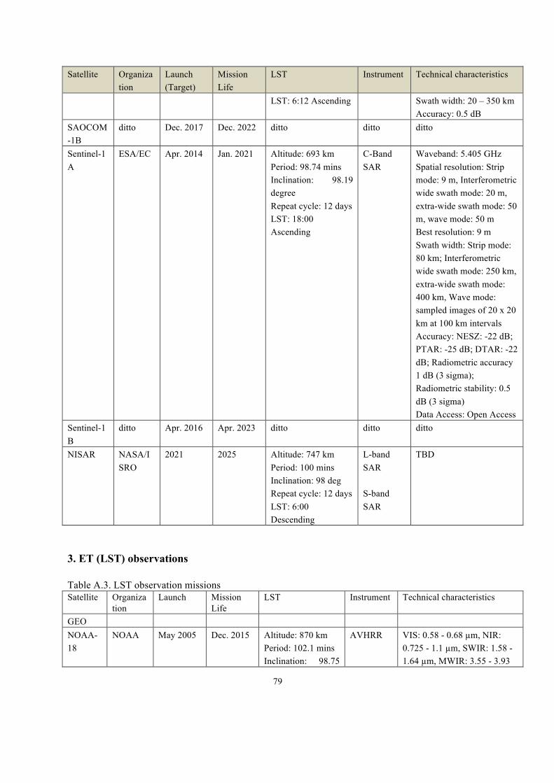
79
Satellite Organization
Launch (Target)
Mission Life
LST Instrument Technical characteristics
LST: 6:12 Ascending Swath width: 20 – 350 km Accuracy: 0.5 dB
SAOCOM-1B
ditto Dec. 2017 Dec. 2022 ditto ditto ditto
Sentinel-1A
ESA/EC Apr. 2014 Jan. 2021 Altitude: 693 km Period: 98.74 mins Inclination: 98.19 degree Repeat cycle: 12 days LST: 18:00 Ascending
C-Band SAR
Waveband: 5.405 GHz Spatial resolution: Strip mode: 9 m, Interferometric wide swath mode: 20 m, extra-wide swath mode: 50 m, wave mode: 50 m Best resolution: 9 m Swath width: Strip mode: 80 km; Interferometric wide swath mode: 250 km, extra-wide swath mode: 400 km, Wave mode: sampled images of 20 x 20 km at 100 km intervals Accuracy: NESZ: -22 dB; PTAR: -25 dB; DTAR: -22 dB; Radiometric accuracy 1 dB (3 sigma); Radiometric stability: 0.5 dB (3 sigma) Data Access: Open Access
Sentinel-1B
ditto Apr. 2016 Apr. 2023 ditto ditto ditto
NISAR NASA/ISRO
2021 2025 Altitude: 747 km Period: 100 mins Inclination: 98 deg Repeat cycle: 12 days LST: 6:00 Descending
L-band SAR S-band SAR
TBD
3. ET (LST) observations Table A.3. LST observation missions Satellite Organiza
tion Launch
Mission Life
LST Instrument Technical characteristics
GEO NOAA-18
NOAA May 2005 Dec. 2015 Altitude: 870 km Period: 102.1 mins Inclination: 98.75
AVHRR VIS: 0.58 - 0.68 µm, NIR: 0.725 - 1.1 µm, SWIR: 1.58 - 1.64 µm, MWIR: 3.55 - 3.93

80
degree LST: 14:00 Ascending
µm, TIR: 10.3 - 11.3 µm, 11.5 - 12.5 µm Spatial resolution: 1.1 km Swath width: approx. 3000 km. Ensures full global coverage twice daily
NOAA-19
NOAA Feb. 2009 Dec. 2015 ditto LST: 14:00 Ascending
ditto ditto
METOP-A
EUMETSAT/NOAA/CNES/ESA
Oct. 2006 Aug. 2018 Altitude: 840 km Period: 107.1 mins Inclination: 98.8 degree Repeat cycle: 29 days LST: 9:30 Descending
ditto ditto
METOP-B
ditto Sep. 2012 Sep. 2017 ditto ditto ditto
METOP-C
ditto Oct. 2018 Oct. 2023 ditto ditto ditto
FY-3A CMA/NRSCC
May 2008 Dec. 2016 Sun-synchronous Altitude: 830 km Period: 101 mins Inclination: 98.753 degree Repeat cycle: LST: 10:10 Descending
VIRR Multispectral Visible and Infra-red Scan Radiometer
10 channels over 0.43 - 10.5 µm VIS, SWIR, MWIR, TIR Spatial resolution: 1.1 km at nadir Best resolution: 1100 m Swath width: 2800 km Accuracy: 1.1 km
FY-3B ditto Nov. 2010 Dec. 2016 ditto LST: 14:00 Ascending
ditto ditto
FY-3C ditto Sep. 2013 Sep. 2016 ditto LST: 10:00 Descending
ditto ditto
FY-3D ditto Dec. 2016 Dec. 2018 ditto LST: 14:00 Ascending
ditto ditto
Terra NASA/METI/CSA
Dec. 1999 Oct. 2019 Sun-synchronous Altitude: 705 km Period: 99 mins Inclination: 98.2 degree Repeat cycle: 16 days
MODIS VIS - TIR: 36 bands in range 0.4 - 14.4 µm Spatial resolution: Cloud cover: 250 m (day) and 1000 m (night), Surface temperature: 1000 m Best resolution: 250 m

81
LST: 10:30 Descending
Swath width: 2330 km Accuracy: Long wave radiance: 100 nW/m2, Short wave radiance: 5%, Surface temperature of land: <1 K, Surface temperature of ocean: <0.2 K, Snow and ice cover: 10%
Aqua NASA/JAXA/INPE
May 2002 Oct. 2019 ditto LST: 13:30 Ascending
MODIS ditto
Landsat 8
USGS/NASA
Feb. 2013 May 2023 Sun-synchronous Altitude: 705 km Period: 98.9 mins Inclination: 98.2 degree Repeat cycle: 16 days LST: 10:11 Descending
TIRS OLI
TIR 10.5 µm and 12 µm TIR Spatial resolution: 100 m Swath width: 185 km Accuracy: Absolute geodetic accuracy of 44 m; geometric accuracy of 32 m or better VIS - SWIR: 9 bands: 0.43 - 2.3 µm Spatial resolution: Pan: 15 m, VIS - SWIR: 30 m Swath width: 185 km Accuracy: Absolute geodetic accuracy of 32 m; relative geodetic accuracy of 18 m (excluding terrain effects); geometric accuracy of 12 m or better
Landsat 9
USGS/NASA
Jan. 2023 Jan. 2033 ditto LST: 10:00
TIRS-2 ditto
NPP NASA/NOAA
Oct. 2011 Sep. 2020 Sun-synchronous Altitude: 824 km Period: 101 mins Inclination: 98.7 degree Repeat cycle: 16 days LST: 13:30 Ascending
VIIRS Waveband: VIS - TIR: 0.4 - 12.5 µm (22 channels) VIS, NIR, SWIR, MWIR, TIR Spatial resolution: 400 m - 1.6 km Best resolution: 400 m Swath width: 3000 km Accuracy: SST 0.35 K
JPSS-1 NOAA/EUMETSAT/NASA
Jan. 2017 Mar. 2024 ditto LST: 13:30 Ascending
VIIRS ditto
JPSS-2 ditto July 2021 July 2028 Sun-synchronous VIIRS ditto

82
Altitude: 833 km Period: 101 mins Inclination: 98.75 degree Repeat cycle: 16 days LST: 13:30 Ascending
Sentinel-3A
ESA/EUMETSAT/EC
Dec. 2015 Dec. 2022 Sun-synchronous Altitude: 814 km Period: 100 mins Inclination: 98.65 degree Repeat cycle: 27 days LST: 10:00 Descending
SLSTR 9 bands in VNIR/SWIR/TIR VIS, NIR, SWIR, TIR Spatial resolution: 500 m (VNIR/SWIR), 1 km (TIR) Best resolution: 500 m Swath width: 1675 km (near-nadir view), 750 km (backward view) Accuracy: 0.2 K abs., 80 mK rel.
ditto OLCI Ocean and Land Colour Imager
Waveband: 21 bands in VNIR/SWIR, VIS, NIR Spatial resolution: 300 m Swath width: 1270 km, across-track tilt 12.2 degree to the West Accuracy: 2% abs, 0.1% rel.
Sentinel-3B
ditto May 2017 Jan. 2024 ditto LST 10:00 Ascending
SLSTR same with Sentinel-3A
ditto OLCI same with Sentinel-3A GCOM-C
JAXA Dec. 2015 Dec. 2021 Sun-synchronous Altitude: 798 km Period: 101 mins Inclination: 98.6 degree Repeat cycle: 3 days LST: 10:30 Descending
SGLI VIS - NIR: 0.38 - 0.865 µm; SW: 1.05 - 2.21 µm; TIR: 10.8 - 12.0 µm Spatial resolution: SGLI-VNR: 250 m, 1000 m; SGLI-IRS: 250 m, 500 m, 1000 m Best resolution: 250 m Swath width: SGLI-VNR: 1150 km; SGLI-IRS: 1400 km
ECOSTRESS
NASA/USGS
2017 2018 Inclined Altitude: 407 km Period: 93 mins Inclination: 51.6 degree Repeat cycle: Ascending
Waveband: TIR TIR Spatial resolution: Swath width: Accuracy:

83
CBERS-4
INPE/CRESDA
Dec. 2014 Dec. 2017 Sun-synchronous Altitude: 778 km Period: 100.3 mins Inclination: 98.5 degree Repeat cycle: 26 days LST: 10:30 Descending
IRS Waveband: 0.5 - 0.9 µm; 1.55 - 1.75 µm, 2.08 - 2.35 µm; 10.4 - 12.5 µm VIS, NIR, SWIR, TIR Spatial resolution: PAN, SWIR: 40 m, TIR: 80 m Swath width: 120 km Accuracy:
CBERS-4A
ditto 2018 2021 ditto ditto ditto
4. River discharge observations Table A.4. River discharge observation missions Satellite Organiza
tion Launch
Mission Life
LST Instrument Technical characteristics
SWOT NASA/UKSA/CNES
2020 2024 Inclined, non-sun-synchronous Altitude: 891 km Period: Inclination: 78 degree Repeat cycle: 22 days
Ka-band Radar Interferometer(KaRIN)
MW, Ka-Band Spatial resolution: Vertical resolution is 2 cm Swath width: Accuracy:
SARAL CNES/ISRO
Feb. 2012 Dec. 2018 Sun-synchronous Altitude: 799 km Period: 100.59 mins Inclination: 98.55 degree Repeat cycle: 35 days LST: 18:00 Descending
AltiKa Waveband: radar altimeter: 35 GHz (Ka-band) Spatial resolution: Swath width: Accuracy:
l Sentinel-3A, B, C
ESA/EC A: Dec. 2025 B:May2017 C:2020
Dec. 2022 Jan. 2024 2027
Type: Sun-synchronous Altitude: 814 km Period: 100 mins Inclination: 98.65 degree Repeat cycle: 27 days LST: 10:00 Asc/desc: Descending
SRAL Waveband: Dual-frequency radar altimeter, Ku-band, C-band Spatial resolution: 300 m Swath width: Profiling Accuracy: 3 cm
Jason-3 NASA/NOAA/CNES/EUMETSAT
Jan. 2016 Jan. 2019 non-sun-synchronous Altitude: 1336 km Period: 112.4 mins Inclination: 66 degree Repeat cycle: 10 days
POSEIDON-3B Altimeter
Waveband: Microwave: Ku-band (13.575 GHz), C-band (5.3 GHz) Ku-Band, C-Band Spatial resolution: Basic
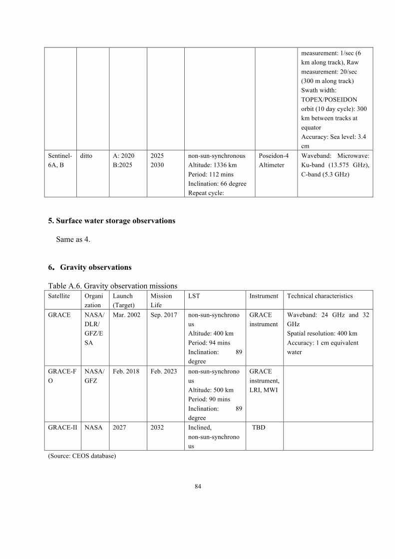
84
measurement: 1/sec (6 km along track), Raw measurement: 20/sec (300 m along track) Swath width: TOPEX/POSEIDON orbit (10 day cycle): 300 km between tracks at equator Accuracy: Sea level: 3.4 cm
Sentinel-6A, B
ditto A: 2020 B:2025
2025 2030
non-sun-synchronous Altitude: 1336 km Period: 112 mins Inclination: 66 degree Repeat cycle:
Poseidon-4 Altimeter
Waveband: Microwave: Ku-band (13.575 GHz), C-band (5.3 GHz)
5. Surface water storage observations
Same as 4.
6.Gravity observations Table A.6. Gravity observation missions Satellite Organi
zation Launch (Target)
Mission Life
LST Instrument Technical characteristics
GRACE NASA/DLR/ GFZ/ESA
Mar. 2002 Sep. 2017 non-sun-synchronous Altitude: 400 km Period: 94 mins Inclination: 89 degree
GRACE instrument
Waveband: 24 GHz and 32 GHz Spatial resolution: 400 km Accuracy: 1 cm equivalent water
GRACE-FO
NASA/GFZ
Feb. 2018 Feb. 2023 non-sun-synchronous Altitude: 500 km Period: 90 mins Inclination: 89 degree
GRACE instrument, LRI, MWI
GRACE-II NASA 2027 2032 Inclined, non-sun-synchronous
TBD
(Source: CEOS database)

85
Appendix B: GCOS/ECV (Source: 2015 Update of CEOS-CGMS Actions in the Response to GCOS IP, May 2015) 5.3.2 Precipitation Importance of this ECV Precipitation affects water supplies, natural vegetation, crops, and tourism. Its variations can lead to environmental hazards in the form of droughts, floods, snow accumulations, hail, and ice. It affects the daily activities of humankind throughout the world. It is a key component of the Earth’s hydrological cycle and, through its release of the latent heat of condensation as it forms, affects the thermal structure and the circulation of the atmosphere. 5.3.2.1 GCOS/CEOS Action A8; SS: A.2 Action: Ensure continuity of satellite precipitation products. Who: Space agencies. Time-Frame: Continuous. Performance Indicator: Long-term homogeneous satellite-based global precipitation products. Annual Cost Implications: 20-40 M US$(for generation of climate products, assuming missions funded for other operational purposes) (Mainly by Annex-I Parties CEOS Entities: · CEOS Agency Leads: NASA, JAXA · CEOS Agency Contributors: NOAA, CSA, CNES, ISRO, INPE, EUMETSAT, ESA · CEOS Coordination Mechanisms: Precipitation Virtual Constellation (PC-VC) International Coordination Bodies: TBD Associated Organizations: TBD Specific Deliverable #1: · The delivery is an initial calibration reference standard for the Global Precipitation Measurement (GPM) mission. The GPM concept centres on the deployment of a “Core” satellite carrying an advanced radar/radiometer system to measure precipitation from space and serve as a reference standard to unify precipitation measurements from a constellation of research and operational satellites. o To ensure the continuity of this constellation approach, NASA/JAXA will continue the Tropical Rainfall Measuring Mission (TRMM) that has both an imaging microwave radiometer, the TRMM Microwave Imager (TMI) and a Precipitation Radar (PR). This observatory is in a 35 deg. inclined orbit. o To extend and enhance the ability to intercalibrate constellation radiometers, NASA/JAXA will launch in 2014, the core observatory of the (GPM mission. This observatory will carry both an imaging microwave radiometer, GPM microwave imager (GMI) and a dual precipitation radar (DPR). This observatory will be in a 65 deg. inclined polar orbit. o JAXA is also contributing the Advanced Microwave Scanning Radiometer-2 (AMSR2) on the Global Change Observation Mission-Water (GCOM-W) to the CEOS PC-VC. Other agencies such as NOAA,

86
EUMETSAT, CNES/ISRO will contribute microwave radiometers in both sun- and non-sun-synchronous orbits (these will be mostly microwave sounders except for Megha-Tropiques, and Special Sensor Microwave Imager/Sounder [SSMI/S] radiometers). While these radiometers are launched and operated for their agencies own needs, they are contributed to the CEOS PC-VC (GPM era constellation) to be included for use in generating consistent precipitation products. o Radiometers in initial GPM-based PC constellation: § SSMI/S F16, F17, F18, F19, F20 microwave imagers containing both window channels and high-frequency sounding channels. Data are observed by the U.S. DOD satellites and archived at NOAA. § Advanced Microwave Sounding Unit (AMSU)-A/Microwave Humidity Sounder (MHS) sounders for precipitation using mainly the scattering channels. Provided by both NOAA and EUMETSAT. § Advanced Technology Microwave Sounder (ATMS) microwave sounders on both Suomi National Polar-orbiting Partnership (Suomi NPP) and Joint Polar Satellite System (JPSS) which for precipitation use mainly the scattering channels. Provided by both NOAA and EUMETSAT. § Microwave Analysis and Detection of Rain and Atmospheric Structures (MADRAS) microwave imager from the CNES/ISRO Megha-Tropiques tropical mission. § Sounder for Probing Vertical Profiles of Humidity (SAPHIR) microwave sounder from the CNES/ISRO Megha-Tropiques tropical mission. SAPHIR provides high- frequency sounding channels for precipitation measurements. o Precipitation Constellation Calibrating Observatory: § During the ad-hoc pre-GPM Precipitation Constellation (PC), the TRMM observatory provides the transfer standard for precipitation products for the PC. This was chosen because of the many match-up opportunities of the TRMM observatory and the polar-orbiting observatories in the constellation. § Beginning with the full PC that starts at the launch of the GPM core observatory in 2014, the GPM core observatory with its GMI and DPR will be the transfer standard used for creating consistent PC precipitation products. Once again the core observatory, like TRMM, provides many match-up opportunities with other observatories in the constellation. · PC characteristics for radiometers in the Constellation o Each PC participating agency will provide a point of contact to the PC about its observatory, radiometer and its operation during the life of the mission. o Each PC participating agency will provide detailed information about the operation, geolocation and calibration of the radiometer that it is providing. o Each PC participating agency will completely characterize their radiometer and calibration and make such information available to other PC members as well as data users. o Each PC participating agency will ensure that incidence angle information is available for each pixel of each swath type for their instrument. · Characteristics of the PC transfer standard observatory o Should contain well-calibrated radiometer with channels from 10 GHz through 183 GHz. o Should contain well-calibrated precipitation radar that represents the state of the art for characterizing rainfall. o Should be placed in a non-sun synchronous orbit to facilitate the number of match-up orbit crossovers between the reference observatory and other observatories in the constellation. o Both calibration and geo-location should be well characterized, tracked, published and the information publicly available.

87
Specific Deliverable #2: · The deliverable is an instantaneous field of view level 1b calibrated, geo-located brightness temperature (Tb) product from each radiometer in the PC. The key to this delivery is the characterization of the inputs to the deliverable and the stability of the calibration and geolocation. Specific Deliverable #3: · The deliverable is a consistent PC instantaneous field of view inter-calibrated brightness temperature (Tc) product from each radiometer in the PC as established by applying the transfer standard established from the GPM core observatory. · Tb products provided by contributors may be calibrated or geo-located according to the needs and requirements of the particular mission. To ensure consistency of PC brightness temperatures all brightness temperatures provided by contributors will be inter-calibrated to meet the standards of this deliverable. Specific Deliverable #4: · The deliverable is a consistent PC precipitation product containing retrievals at instantaneous field of view based upon PC consistent inter-calibrated Tc. Also, to ensure consistency the retrieval will be based on a well-established Bayesian technique using a physically based a priori database constructed from the combined radiometer/radar measurement from the PC GPM core observatory. At latitudes for which the reference observatory measurements are not available, other physical measurements such as those from ground radars, cloud radars and other appropriate physical sources should be used before reverting to profiles generated from cloud resolving models. · This precipitation retrieval will be performed for all radiometers in the PC. A similar retrieval based on a physically based a priori database will be made from imager and sounder radiometers. Appropriate retrievals will be made over ocean, land and coast. Specific Deliverable #5: · This deliverable provides a global monthly product containing PDF of precipitation intensity based on the instantaneous field of view (IFOV) products delivered in the previously listed deliverable #4. · While this deliverable is not the end product of the ECV, it is the satellite component that appears most useful for further synthesis with other products. Accuracy, stability, horizontal resolution, and vertical resolution
ECV: Precipitation
GCOS/CEOS Action A8 Property Instantaneous
FOV Tb Instantaneous FOV inter- calibrated Tb
Precipitation rate (Instantaneous FOV)
Precipitation rate (Monthly)
Accuracy Target TBD TBD TBD max(10% of daily totals; 0.1 mm)
Planned TBD 0.3 K for each radiometer in the constellation with respect to the reference radiometer
TBD TBD

88
Stability Target TBD TBD TBD 5% of daily totals (regional scale)
Planned 1 K TBD TBD TBD Horizontal resolution (km)
Target TBD TBD TBD 25 Planned 5 (Precip.Radar) 25 25 100
Vertical resolution (km)
Target TBD N/A N/A N/A Planned 0.25 (Precip.
Radar) N/A N/A N/A
Planned activities/time frames to meet deliverables (2011 – 2015) TBD 2015 Update Specific Deliverable #1 • TRMM has continued to be operated; it is out of fuel and will be passivized in early 2015 when its orbit decays to a set altitude (325 km). The TMI is operating continuously, while the radar is only available when the altitude is in set ranges. • GPM was launched into a 65° orbit on 27 February 2014 (UTC), and Day-1 GMI and DPR products were released in stages through the summer. • The initial GPM-era constellation consists of microwave imagers (DMSP F15 SSMI [limited]; DMSP F16, F17, F18, and F19 SSMIS; TRMM TMI; GCOM-W1 AMSR2; GPM GMI) and microwave sounders (NOAA-18, NOAA-19, Metop-A, and Metop-B MHS; Megha-Tropiques SAPHIR; SNPP ATMS). • The pre-GPM PC calibrator was the TRMM observatory; it is planned that intercalibration of the TRMM and GPM observatories will allow the entire TRMM-GPM era to be treated as a continuous record, a long time series that is now viewed as critical for the long-term records demanded for societal applications, including climate studies. • Upon reflection, “completely characterize” seems unachievable for sensors; “carefully” is a reasonable standard that agencies strive to achieve. Specific Deliverable #2 The satellite operators work through GSICS to ensure calibration and geolocation at Level 1b. Specific Deliverable #3 The GPM project’s XCal Team developed and maintains intercalibrations of all radiometers to the Core Observatory reference at Level 1c. Specific Deliverable #4 GPM is developing a physically based Bayesian retrieval system that can be applied to both imagers and sounders, GPROF2014, which is designed to be useful over land, coast, ocean, and frozen surfaces. Independently, NOAA is pursuing a more assimilation-like approach that applies to both imagers and sounders, MiRS. Specific Deliverable #5

89
The output of GPROF2014 applied to all the microwave sensors in the constellation is freely available as individual satellite orbits at Level 2 – IFOVs in the original scan/footprint coordinates. Additional Comments 1. Computations of the precipitation ECV rest not only on the microwave constellation currently considered the CEOS-VPC, but also on the geosynchronous constellation that provides increasingly rich multi-spectral data on relatively fine time intervals. As such, “the constellation” the community needs really encompasses both sets of satellites. 2. The future of the microwave constellation (and even the Indian Ocean segment of the geo-constellation) is open to question. It takes a decade or more to carry a satellite from concept to launch, so it seems essential to have a planning activity as part of the 5-year plan. One can’t open discussions at the end of one 5-year period and assume that satellites will appear to fill the need as legacy satellites age off of the system. 3. The current statement on the necessary number of microwave constellation satellites is that we need the time between observations to be no more than 3 hours. That’s not an average, that’s the maximum. The current uncoordinated collection of satellites makes it hard to achieve this, but we should go for some standard like “75% of gaps be <3 hours”. Reference 5.5.4 Soil Moisture Importance of this ECV Soil moisture is an important variable in land-atmosphere feedbacks because of its major effect on the partitioning of incoming radiation into latent and sensible heat and on the allocation of precipitation into runoff, subsurface flow, and infiltration. Soil moisture is intimately involved in the feedback between climate and vegetation, since local climate and vegetation both influence soil moisture through evapotranspiration, while soil moisture and climate determine the type of vegetation in a region. Soil moisture estimates can also assist gas flux estimates in permafrost regions. As a climate impact variable, soil moisture affects agricultural and natural vegetation productivity, the likelihood of flash floods, the management of agricultural and city water, and the spread of vector-borne diseases such as Dengue fever and malaria. 5.4.1 GCOS/CEOS Action T13; SS: T.11 Action: Develop a record of validated globally-gridded near-surface soil moisture from satellites. Who: Parties’ national services and research programmes, through GEWEX and TOPC in collaboration with space agencies. Time frame: 2014. Performance indicator Availability of globally validated soil moisture products from the early satellites until now. Annual Cost Implications: 1-10 M US$ (10% in non-Annex-I Parties). CEOS Entities: · CEOS Agency Leads: ESA · CEOS Agency Contributors: EUMETSAT, NASA

90
· CEOS Coordination Mechanisms: TBD International Coordination Bodies: International Soil Moisture Working Group (ISMWG), GEWEX, TOPC, WCRP Data and Assimilation Committee (WDAC) Associated Organizations: TBD Specific Deliverable(s): · 30+ years surface soil moisture data record derived from active (European Remote Sensing Satellite-2 [ERS-2] scatterometer, Metop Advanced Scatterometer [ASCAT]) and passive (Scanning Multichannel Microwave Radiometer [SMMR], TMI, Advanced Microwave Scanning Radiometer – EOS [AMSR-E], Windsat, SSM/I) microwave observations. Unit will be in volumetric soil moisture (m3m-3) and alternatively in degree of saturation (%). ESA projects Water Cycle Observation Multi-mission Strategy (WACMOS) (http://wacmos.itc.nl/) and ESA's Climate Change Initiative (CCI - the soil moisture project) recently begun in December 2011. Accuracy, stability, horizontal resolution, and vertical resolution
ECV: Soil moisture
GCOS/CEOS Action T13 Property Soil moisture
Accuracy (m3m-3)
Target 0.04 Planned 0.08, Variable, dependent on land cover
Stability (m3m-3 per year)
Target 0.01 Planned 0.01, Variable, dependent on land cover
Horizontal resolution (km)
Target 50 Planned 100 km, Variable over time
Key activities and time frames to meet deliverables (2011 – 2015) · Completion of the ESA project WACMOS (early-mid 2012) · Climate Change Initiative (CCI) Soil Moisture project (12/2011-11/2014) 2015 Update
• The successful completion of the ESA project WACMOS in 2012 provided the functional design of the CCI SM production system.
• Building upon the work undertaken in WACMOS, in collaboration with ESA’s CCI SM project, June 2012 saw the release of the first 30+ year, global, soil moisture project derived from active and passive EO data sets.
• The third data set (product) release of CCI SM v02.1 was made in Sept 2014 providing 35 years of data from 1978 onwards, and is freely available, after registration, via http://www.esa-soilmoisture-cci.org/
• As provided in the recently authored Product Validation and Intercomparison Report (Nov 2014), available from CCI SM web site (Jan 2015), the CCI SM data set has been successfully, independently, validated and compared against in situ, modelled and other satellite datasets.
• A review of the CCI phase 1 SM product in January 2014, using the modified bates maturity

91
index of the CORE-CLIMAX project, resulted in an overall score of 3 (Initial Operations Capacity).
• Since the first product release in 2012 more than 1200 users have registered to date to obtain the product. The product enjoys a global uptake with the majority of users coming from the USA, China and India, and a strong following across the EU, and Australasia. The users focus largely on Climate, Water and Ecosystem issues, although Disaster and Agriculture are also key topics
• Following the successful completion of CCI SM phase 1 in Dec 2014, phase 2 (CCI SM 2) will start on 1.1. 2015, running to 31.12.2017 and, in close collaboration with user groups, sees the graceful evolution of the implementation of the production system towards an operational system.
5.5.3 Lakes Importance of this ECV The world’s 150 largest lakes contain 95% of the water in all the world’s lakes. Most of these large lakes are hydrologically open. The volume of water in lakes reflects both atmospheric (precipitation, evaporation-energy) and hydrological conditions (surface-water recharge, discharge and ground-water tables). Observing lake freeze-up and break-up dates is an important indicator for climate change in boreal and polar regions. 5.5.3.1 GCOS/CEOS Action T8; SS: T.1.1 and T.1.2 Action: Submit weekly/monthly lake level/area data to the International Data Centre; submit weekly/monthly altimeter-derived lake levels by space agencies to HYDROLARE. Who: National Hydrological Services through WMO CHy, and other institutions and agencies providing and holding data; space agencies; HYDROLARE. Time-Frame: 90% coverage of available data from GTN-L by 2012. Performance Indicator: Completeness of database. Annual Cost Implications: 1-10 M US$ (40% in non-Annex-I Parties). CEOS Entities: · CEOS Agency Leads: CNES · CEOS Agency Contributors: NASA, NOAA, ESA, ISRO, EUMETSAT · CEOS Coordination Mechanisms: TBD International Coordination Bodies: TBD Associated Organizations: TBD Specific Deliverable(s): · Standardized long-term and near-real time surface water height variations from the historical and current suite of satellite radar altimeters. Data should include target location (central latitude/longitude), type (natural or man-made impoundment such as open/closed/ephemeral lake and reservoir), time of measurement, average height, height error, reference frame, mean radar backscatter coefficient and/or freeze/thaw indicator, correction matrix. The matrix should describe which altimetric range and height corrections have been applied, and their assumed errors. · Standardized long-term and near real time lake surface extent derived from satellite imaging

92
instruments. Accuracy, stability, horizontal resolution, and vertical resolution
ECV: Lakes
GCOS/CEOS Action T8 Property Lake level Lake area
Accuracy
Target 50 cm 5% Planned 10 cm 5%
Stability (%/decade)
Target 10 cm 5 Planned TBD TBD
Horizontal resolution (km)
Target N/A 0.25 Planned TBD TBD
Key activities and time frames to meet deliverables (2011 – 2015) · Require a high resolution map showing location of world’s lakes. · Require international consensus and cooperation’s on formation and implementation of any global database. · Requires formation of dedicated team to ingest, assemble and deliver lake level products. Near real time applications will require system automation with some manual oversight. 2015 Update Lake level was routinely reported by the ENVISAT altimeter until the end of the mission in May 2012. Lake levels are currently reported by the ISRO Satellite with ARgos and ALtiKa (SARAL) mission.

93
Appendix C: WMO SOG-Hydrology and Water Resources Precipitation Various meteorological variables including precipitation depth and type are routinely observed on an hourly to daily basis at synoptic weather stations. Global coverage from in-situ observations exhibit large regional differences. Exchange of data is achieved in real-time and near real-time mode and subsets of the precipitation measurements made are accessible through global networks and data centres. Increasingly, spatial and temporal coverage of rainfall observations is improving using ground radar techniques. Satellite observations from on-board radars as well as microwave imagers and sounders are also of value and enable precipitation information to be derived on a global scale. Merged data products using direct terrestrial observations and satellite observations are routinely available at the global scale. However, quantitative precipitation observations from satellite measurements at present do not meet accuracy requirements; but when combined with terrestrial observations they provide precipitation estimates with an improving resolution. Information from TRMM satellites and the emerging precipitation network through the virtual constellation network of CEOS provide improved precipitation information that can be used flood forecasting. Major progress is expected from the Global Precipitation Mission (GPM). There is a focus on improving satellite and radar based rainfall information in real-time for use in flash flood forecasting. This is operationally achieved by making use of hydrological S-band Doppler radars and improved satellite-based observations. As quantitative precipitation forecasting using S-Band Hydrological Radars increase in popularity especially for flash flood forecasting in many countries, improved guidance for calibration and intercomparison of accuracies is required. With regard to satellite-based quantitative precipitation estimation, a mechanism is required to develop front-end products and mainstream precipitation products for operational day-to-day use in National Hydrological Services on a long-term basis. Soil Moisture The observation of soil moisture or soil wetness (as a proxy for soil moisture) is important for hydrological forecasting in large river basins and likewise for modelling of the land surface module in coupled land-atmosphere models. A number of networks for soil moisture measurements exist in different parts of the globe. The identification of a global in-situ network on soil moisture is in an advanced planning stage. This will involve network enhancement by expansion and standardization, dedicated soil moisture missions (support for SMOS, ESA’s soil moisture ocean salinity satellite mission), and improved coordination of soil moisture data network planning, observing standards, and data exchange. The use of advanced scatterometers allows derivation of soil wetness of the first few centimetres that however is only partially useful for hydrological studies and forecasting and need to be augmented by infiltration models, for example. On terrain, soil wetness can also be observed by passive microwave emission radiometry. On a global scale, with a spatial resolution of about 30-50 km, L-Band radar may provide spatial coverage. On a regional basis, a soil moisture index for Europe and Africa is derived from meteorological satellite data; this work is done within the framework of the EUMETSAT Satellite Application Facility for Land Surface Analysis (Land-SAF). Most of the active and passive microwave instruments provide some soil moisture information for regions of limited vegetation cover. However, under many conditions remote-sensing data are inadequate, and information regarding moisture depth remains elusive. Unfortunately, none of the instruments provide a satisfactory combination of spatial resolution and repeat cycle time (2 to 3 days). The AMSR data comes close to providing soil moisture or land wetness information that may be marginally useful for meso-scale models but the timeliness of these data remains challenging.
94
Satellite coverage provides information on the state of the land and on land processes. This information is of considerable benefit for agriculture; forestry; surface transport management, and the monitoring of ecological and hydrological systems. The Surface Soil Moisture L2 product is derived from the Advanced Scatterometer (ASCAT) data and given in swath geometry. This product provides an estimate of the water saturation of the 5 cm topsoil layer, in relative units between 0 and 100 [%]. The algorithm used to derive this parameter is based on a linear relationship of soil moisture and scatterometer backscatter and uses change detection techniques to eliminate the contributions of vegetation, land cover and surface topography, considered invariant from year to year. Seasonal vegetation effects are modelled by exploiting the multiple viewing capabilities of ASCAT. The ASCAT surface soil moisture product is thus the first truly operational satellite soil moisture product that may be used for Numerical Weather Prediction (NWP), flood forecasting and other time-critical applications. Surface Water Discharge Discharge is typically calculated at a particular location in a river, but represents the water running off from the entire catchment into the river above that location. It is derived from a measured water level (stage) converted to discharge by means of a rating curve developed for the particular channel cross-section at which the water level is measured, or by more accurate-theoretical methods where possible (e.g. rated weirs. Rating curves can be theoretically derived, but are generally empirically developed from a series of discharge measurements, and then extended graphically to flows at stage heights for which the discharge has not been measured. Flow in a channel can be influenced by factors such as changes in land use, withdrawal for water use, or contributions from artificial water storage reservoirs; thus, weather is not the only variable affecting discharge. The quality of discharge measurements is also impacted by unstable controls at the measuring point and in some cases tidal influences. On a global scale, terrestrial hydrological observations are not available for all catchments and are generally unavailable or of poor quality in remote and mountain areas. Access to hydrological data is often impeded by a number of factors including fragmentation of data holdings at the national level and access restrictions. Two new approaches to global monitoring are the planned implementation of the Hydrological Applications and Runoff Network (HARON) in cooperation with the WMO, GCOS, GRDC and facilitated by GEOSS and the WMO Commission for Hydrology proposal for a WMO Hydrological Observing System (WHOS). Likewise, the WMO’s WHYCOS Programme contributes to the improvement of surface hydrological networks, but usually based on a specific need for hydrological information, such as flood forecasting and warning or water resources management. On a local basis, satellite derived water-level observations based on altimeters are available for some large rivers and can now be utilized for major basins (wide rivers) and lakes in a quasi-operational mode. The quality of such observations is yet to be fully determined and in-situ observations for calibration are essential. Several satellite-based methods are available on demand to map the extent of flooding in floodplains or large riverine systems as well as the duration of flooding, including visual, IR and radar sensors. However, in general, hydrological observations from spacecraft are not available for any given location on a daily basis owing to the geometry of spacecraft orbits. In most instances, it may only be possible to obtain data once every two to three weeks at a specific location which is a serious constraint. Surface water storage This variable is directly related to the volume of freshwater stored in lakes, reservoirs and wetlands. Again storage volume is usually derived by measuring the height of the water in the lake or reservoir and then converting this to a volume using a height versus storage volume curve derived from elevation data or information on the topography beneath the water body. There is also the issue of water storage in river channels, flood plains and large estuaries which is more of a challenge to measure continuously. While terrestrial

95
observations are being made for lakes and reservoirs (levels of lakes and reservoirs, volumetric observations), space-based observations such as those derived from altimetric observations are also becoming more readily available. However, these are water level elevation values only and, without the relevant storage height-volume curves, do not provide information on the actual amount of water within the lake or reservoir. Generally, observations are not yet available for wetlands, large floodplains and estuaries. This may change with improved digital elevation data. The availability of surface water storage fluxes for the major lakes and reservoirs would contribute to a more accurate modelling of lateral fluxes in climate circulation models. The fluxes would be best derived from the storage volume data rather than changes in height only. Presently, the ability of the ICES/GLAS instrument to provide accurate measurements of lake levels is being tested. Again, in-situ records are invaluable. However, many observational uncertainties still exist with regard to flow retention in dams, reservoirs, lakes and wetlands; the evaporative loss of water from storage surfaces; and seepage to groundwater stores. Groundwater storage Groundwater storage is also a difficult variable to measure as usually it is the height of the groundwater level that is recorded and the volume/water availability derived from pump testing and geographical analyses. Groundwater fluxes have a major influence on the dynamics of the global hydrological cycle as they represent water coming back into the surface water realm through pumping or springs and also water flowing from the surface water to groundwater via recharge of aquifers. Because groundwater tends to respond more slowly to short-term climatic variations than surface water resources, this variable is often not considered to be of first-order importance from a climate perspective. However, in fact, its long term nature does lend it to be of importance in longer time scale analyses. Terrestrial observations are being made but overall global access to groundwater data (rates of recharge and abstraction in particular) is highly limited. IGRAC has compiled global level information on groundwater resources. Gravimetric observation techniques (such as from GRACE) for very large groundwater bodies are available but yet to be fully proven in operational circumstances. The use of GOCE data is being explored.

96
Appendix D: List of Acronyms AAFC Agriculture and Agri-Food Canada AGPI TRMM Adjusted Geostationary Operational Environmental Satellite
Precipitation Index AIRS Atmospheric Infrared Sounder ALEXI Atmosphere-Land Exchange Inverse model ALOS Advanced Land Observing Satellite AMSRE, AMSR2 Advanced Microwave Scanning Radiometer 2 AMSU Advanced Microwave Sounding Unit ASCAT Advanced Scatterometer ASTER Advanced Spaceborne Thermal Emission and Reflection radiometer ATMS Advanced Technology Microwave Sounder CALDAS Coupled land and atmosphere data assimilation system CAMS Climate Anomaly Monitoring System CBERS China–Brazil Earth Resources Satellite program CCI Climate Change Initiative CEOS Committee on Earth Observation Satellites CEOS EO DB CEOS Earth Observation Database CGMS Coordination Group for Meteorological Satellite CHy WMO Commission for Hydrology CLM Community Land Model CNES Centre National d'Études Spatiales CONUS Continental United States CoP Community of Practice CORE-CLIMAX COordinating Earth observation data validation for RE-analysis for CLIMAte
ServiceS CPC Climate Prediction Center CSA Canadian Space Agency DHM Distributed hydrological models DMSP Defense Meteorological Satellite Program DPR Dual-Frequency Precipitation Radar DSWE USGS Dynamic Surface Water Extent DVM Dynamic Vegetation Model EC Environment Canada ECOSTESS ECOsystem Spaceborne Thermal Radiometer Experiment on Space Station ECV Essential Climate Variables ENVISAT Environmental Satellite EOS Earth Observing System ESA European Space Agency ET Evapotranspiration EU European Union EUMETSAT European Organisation for the Exploitation of Meteorological Satellites EWV Essential Water Variables FAS USDA Foreign Agricultural Service FFGS WMO Flash Flood Guidance System

97
FS Feasibility Study FY FENGYUN Satellite GCOM, GCOM-W1 Global Change Observation Mission GCOS Global Climate Observing System GEO Group on Earth Observations GEOSS Group on Earth Observations System of Systems GES DISC Goddard Earth Sciences Data and Information Services Center GET-D GOES Evapotranspiration and Drought GEWEX Global Energy and Water cycle Exchanges GGMN Global Groundwater Monitoring Network GLAS Geoscience Laser Altimeter System GLDAS Global LDAS GMI GPM Microwave Imager GOCE Gravity field and steady-state Ocean Circulation Explorer GOES Geostationary Operational Environmental Satellite GPCP Global Precipitation Climatology Project GPI Gemini Planet Imager GPM Global Precipitation Measurement GRDC Global Runoff Data Centre GRIDSAT Gridded Satellite GSFC Goddard Space Flight Center GRACE Gravity Recovery and Climate Experiment GRACE-II Gravity Recovery and Climate Experiment II GRACE FO GRACE Follow-On GTN-L Global Terrestrial Network Lakes GW Groundwater HARON Hydrological Applications and Runoff Network HRC WMO Hydrologic Research Centre HSB Humidity Sounder for Brazil HYDROLARE International Data Centre on Hydrology of Lakes and Reservoirs ICESat Ice, Cloud, and land Elevation Satellite IEM Integral Equation Model IFOV Instantaneous field of view IGRAC International Groundwater Resources Assessment Centre IGWCO Integrated Global Water Cycle Observations INPE Brazilian National Institute of Space Research INSAR Interferometric synthetic aperture radar IP Implementation Plan IR Infrared IRWIN Infrared window ISMWG International Soil Moisture Working Group ISRO Indian Space Research Organisation ISS International Space Station JAXA Japan Aerospace Exploration Agency JPSS Joint Polar Satellite System LANCE NASA Land, Atmosphere Near real-time Capability for EOS

98
Land-SAF EUMETSAT Satellite Application Facility for Land Surface Analysis LANDSAT LDAS Land Data Assimilation Systems LEO Low Earth orbit LSI-VC CEOS Land Surface Imaging Virtual Constellation LSM Land Surface Models LST Land Surface Temperature MADRAS Microwave Analysis and Detection of Rain and Atmospheric Structures MERRA Modern Era Retrospective-Analysis for Research and Applications MHS Microwave Humidity Sounder MODIS Moderate Resolution Imaging Spectroradiometer MSU Microwave Sounding Unit MTG Meteosat Third Generation MW Microwave MWI Microwave Imager MWS Microwave Sounder NASA National Aeronautics and Space Administration NCEP National Centers for Environmental Prediction NESDIS National Environmental Satellite, Data, and Information Service NLDAS North American LDAS NMHS National Hydrological and Meteorological Service NOAA National Oceanic and Atmospheric Administration NPP Suomi National Polar-orbiting Partnership NRC National Research Council NWP Numerical Weather Prediction NWS National Weather Service OLCI Ocean and Land Colour Instrument OPI OLR Precipitation Index PC Precipitation Constellation PPS Precipitation Processing System PR Precipitation Radar P-VC CEOS Precipitation Virtual Constellation RCM RADARSAT Constellation Mission RD River Discharge RTM Radiative transfer model SAPHIR Sounder for Probing Vertical Profiles of Humidity SAR Synthetic Aperture Radar SARAL Satellite with ARgos and ALtiKa SBA Societal Benefit Area SDG Sustainable Development Goals SGLI Second generation Global Imager SLSTR Sea and Land Surface Temperature Radiometer SM Soil moisture SMAP Soil Moisture Active Passive mission SMOPS Soil Moisture Operational Products System SMOS Soil Moisture and Ocean Salinity mission

99
SNPP Suomi-National Polar-Orbiting Operational Environmental Satellite System Preparatory Project
SoG WMO Statement of Guidance SoG-H WMO Statement of Guidance for Hydrology SSM/I Special Sensor Microwave Imager SSMIS Special Sensor Microwave Imager/Sounder SSMR Scanning Multichannel Microwave Radiometer ST Storage SWE Snow Water Equivalent SWOT Surface Water Ocean Topography TCI Temperature Condition Index TIR Thermal Infrared Remote Sensing TIROS Television InfraRed Observational Satellite TMI TRMM Microwave Imager TMPI Threshold-Matched Precipitation Index TOPC Terrestrial Observation Panel on Climate TOVS TIROS Operational Vertical Sounder TRMM Tropical Rainfall Measuring Mission USAID United States Agency for International Development USDA United States Department of Agriculture USGS United States Geological Survey VIIRS Visible Infrared Imaging Radiometer Suite WACMOS Water Cycle Multi-mission Observation Strategy WCOM Water Cycle Observation Mission WCRP World Climate Research Programme WDAC WCRP Data and Assimilation Committee WHOS WMO Hydrological Observing System WHYCOS World Hydrological Cycle Observing System WMO World Meteorological Organization WOFS Water Observations from Space WSIST Water Strategy Implementation Study Team