ISSN 2042-2695

CEP Discussion Paper No 1542

April 2018

The Billion Pound Drop: The Blitz and Agglomeration Economics in London

Gerard H. Dericks Hans R.A. Koster

Abstract This paper exploits locally exogenous variation in the location of bombs dropped during the Blitz to quantify the effect of density restrictions on agglomeration economies in London: an elite global city. Employing microgeographic data on office rents and employment, this analysis points to effects for London several multiples larger than the existing literature which primarily derives its results from secondary cities. In particular, doubling employment density raises rents by 25%. Consequently if the Blitz had not taken place, the resulting loss in agglomeration economies to present day London would cause total annual office rent revenues to fall by $4:5 billion equivalent to 1:2% of London's annual GDP. These results illuminate the substantial impact of land-use regulations in one of the world's largest and most productive cities.

Key words: regulatory costs, office rents, agglomeration economies, London Blitz bombings. JEL: R14; R33; R38

This paper was produced as part of the Centre’s Urban and Spatial Programme. The Centre for Economic Performance is financed by the Economic and Social Research Council.

This work has benefited from a VENI research grant from the Netherlands Organisation for Scientific Research and a Data-without-Boundaries grant (European Union's Seventh Framework Programme). We thank Catherine Emma Jones, the University of Portsmouth and bombsight.org for providing data on the locations of Blitz bombings. Simon Abele and Balthasar Petrelli are thanked for providing assistance with the geographical data. We thank Paul Cheshire, Frederico Curci, Steve Gibbons, Christian Hilber, Or Levkovich, Steve Redding, Stuart Rosenthal, Tate Twinam, Jos van Ommeren, and seminar participants in Barcelona, Lisbon, London, Oxford, and Portland for for useful comments.

Gerard H. Dericks, Smith School of Enterprise and the Environment, University of Oxford. Hans R.A. Koster, Department of Spatial Economics, Vrije Universiteit Amsterdam, and Centre for Economic Performance, London School of Economics.

Published by Centre for Economic Performance London School of Economics and Political Science Houghton Street London WC2A 2AE

All rights reserved. No part of this publication may be reproduced, stored in a retrieval system or transmitted in any form or by any means without the prior permission in writing of the publisher nor be issued to the public or circulated in any form other than that in which it is published.

Requests for permission to reproduce any article or part of the Working Paper should be sent to the editor at the above address.

G.H. Dericks and H.R.A. Koster, submitted 2018.

1 Introduction

Cities are engines of economic growth. Scholars have long recognized that this enhanced

productivity appears to be heavily dependent upon the built environment – particularly the scale

and density of economic activity. However once cities’ spatial structures have been established,

they are difficult to modify. This sluggishness of change is understood to reflect the presence

of so-called ‘density frictions’. Although density frictions may arise from a variety of sources

including the inherent durability of the building stock, in many if not most cities the primary

density friction is thought to be regulation.

A common class of such regulations is density restrictions – particularly building height limits.

Such restrictions may not necessarily reduce social welfare, as they may be a means to mitigate

various externalities such as traffic congestion and incompatible land uses (Brueckner 2000).

Density restrictions may also protect amenities and increase the quality of the built environment,

implying a positive effect on land prices. However, many planning regulations limiting density

have grown historically and do not adjust to changes in local demand (Cheshire 2009). Therefore

regulatory hurdles pose perhaps the greatest obstacle to more compact urban growth (Cheshire

& Sheppard 2002, Glaeser et al. 2005, Glaeser & Gottlieb 2009, Hilber & Vermeulen 2016).

London, the city on which we focus this paper, is a particularly interesting case. Cheshire &

Hilber (2008) show that London can be considered the world’s most restrictive major office

market – and far more restrictive than any market in the United States. Yet within London

there are substantial local differences in land-use restrictions. For example, London’s West End

submarket is much more restrictive than the City of London or Canary Wharf, ostensibly due

to its history and abundance of cultural amenities. Employment densities in the West End are

consequently considerably lower than in London’s other submarkets.

Density frictions in commercial real estate markets generally constrain employment densities,

which implies that the potential to interact with other workers and benefit from agglomeration

economies is less than if there were no frictions prohibiting firms from greater clustering.

Agglomeration economies arise due to labour market pooling, input and output sharing, and

knowledge spillovers (Marshall 1890), and appear to be highly dependent on the density of

economic activities (Ciccone & Hall 1996, Rosenthal & Strange 2003, Ahlfeldt et al. 2016). These

1

advantages seem to explain why rent for a unit of office space in elite global cities like London,

New York, and Tokyo are several multiples above their corresponding national averages. As

a global financial center, London is not only a major host to industries which greatly benefit

from higher local densities, but also to some of the world’s most innovative firms and people.

In the presence of such potentially large agglomeration economies it has been suggested that

governments should encourage rather than prohibit the clustering of firms within cities (Rossi-

Hansberg 2004). At the very least, an understanding of the economic effects of density in these

high productivity locations is essential to beginning the policy debate.

However, several endogeneity issues make identification of the economic effects of density

challenging. Height constraints and density, for example, could be directly influenced by

prices (see Hilber & Robert-Nicoud 2013). In this study we address this issue by using a

quasi-experimental setting based on the Blitz bombings, which erased a substantial portion of

London’s building stock at the time.1 We use the local concentration of the bombs dropped

during the Blitz as an exogenous proxy for the permissiveness of present day local regulation. We

demonstrate the validity of this proxy with suggestive evidence that planning applications are

indeed less likely to be rejected and that buildings are taller in more heavily bombed areas. A

concern with this methodology is that the location of bombings may not be completely random

over space, and therefore may be correlated with centrality or local amenities. To address this

concern, we present both anecdotal and rigorous statistical evidence that the locations of Blitz

bombings were indeed random at our local scale of analysis.

Because higher densities increase the potential for agglomeration economies, we hypothesize that

greater Blitz bomb densities should now be associated with higher productivity and higher land

values. This is consonant with an emerging literature showing that within-city differences in

agglomeration economies are an important determinant of various economic outcomes including;

firm location choice (Arzaghi & Henderson 2008), land prices (Ahlfeldt et al. 2016), property

prices (Cheshire & Dericks 2014), and rents (Koster et al. 2014), and that these effects appear to

attenuate rapidly with distance. Furthermore, the capitalization of this enhanced productivity

into local price differentials should be even greater for locations with tight supply constraints such

1For instance, it is estimated that a third of the buildings in the City of London were destroyed (Marriott1989, p.66)

2

as London (Sivitanidou & Wheaton 1992, Rosenthal & Strange 2004). We then use the locally

random Blitz bombings as an instrument for current employment density, thereby demonstrating

the particularly strong effect that agglomeration economies within London have on office rents.

This paper makes a number of contributions to the literature on the economic effects of land

use regulation and the measurement of agglomeration economies. While the economies of the

developed world have ostensibly been liberalized over the past several decades, land use regulation

has by contrast generally expanded and intensified (McLaughlin 2012). Although the current

empirical literature on the economic effects of land use regulation focuses almost entirely on the

housing market (see Hornbeck & Keniston 2017, Turner et al. 2014, Siodla 2015), such restrictions

would seem much more important in the context of commercial property, whose high-rise office

buildings dominate most CBDs.2 Similar to only a few recent studies of agglomeration economies,

we employ actual transactions of commercial office rents for individual buildings as our dependent

variable.3 Although using wage data is most common, office rents are arguably the best economic

manifestation of agglomeration economies arising from service industries in urban areas (Drennan

& Kelly 2011, p.488). We also compare our results derived from office rents with those from

house prices – a commonly used proxy for commercial rents within the agglomeration economies

literature – and show that this substitution may underestimate the true magnitude of the effects.

Furthermore, we examine London exclusively, and at a microgeographic scale, thereby producing

specific estimates for the level of agglomeration economies operative within the one of the world’s

largest and most productive cities. No previous research on agglomeration economies has utilized

transactions-based commercial data at such a fine spatial scale and in a city of comparable size

and sophistication to London. We also show that within London agglomeration economies seem

to extend for some distance beyond the immediate location of firms (at least 1 km).

In addition, our results contribute to the still limited stream of research within the broader

agglomeration literature that has employed exogenous sources of variation in employment density.

However, unlike some previous research we are able to objectively demonstrate the conditional

exogeneity of our instrument: Blitz bombings. We achieve this by adapting the industrial

localization metric of Duranton & Overman (2005) to rigorously test for the spatial randomness

2As an illustration, of London’s 10 tallest buildings only one is classified as residential.3see for example Koster et al. (2014) and Liu et al. (2016)

3

of Blitz bomb strikes. Employing historical war damage as a source of exogenous variation has

become increasingly common in empirical work addressing challenging econometric questions.

For example, using wartime bombings as a proxy for economic shocks, Davis & Weinstein (2002),

Brakman et al. (2004), and Bosker et al. (2007) show that enduring location-based natural

advantages maintain the relative economic status between cities over the long-run. Whereas,

akin to this study, Koster & Rouwendal (2012) and Redding & Sturm (2016) investigate the

long-run impact of war damage within cities.

Our results point toward a strong and negative net effect of density frictions on office rents: a

one standard deviation increase in bomb density leads to an increase in rents of about 8.5%.

Additionally, we show that agglomeration economies are a key determinant of office rents in elite

cities: the elasticity of rents with respect to agglomeration appears to be about 5 times as large

as that commonly measured for wages, and half again to twice as large as previous estimates

using rents primarily derived from regional and other secondary cities. Back-of-the-envelope

calculations highlight the importance of density frictions: if the Blitz bombings had not taken

place, employment density would be about 50% lower and the resulting loss in agglomeration

economies would lower total revenues from office space in Greater London by about £4.5 billion

per year, equivalent to 1.2% of Greater London’s GDP or 39% of its average annual growth

rate.4

This paper proceeds as follows. In Section 2, we summarize the expected effects and provide a

background on the importance of density frictions and agglomeration economies in the London

office market and discusses the London Blitz. Section 3 provides evidence that the Blitz

bombings are (conditionally) random at our local scale of analysis, and correlates the location

of bombings with current density restrictions. Section 4 introduces the data used and outlines

the econometric framework. Section 5 discusses the results, followed by a sensitivity analysis –

including substituting office rents with house prices in Section 6. Section 7 concludes.

4Average annual growth rate for Greater London 1999–2016 is 3.0%: sourced from ONS

4

2 Research context

2.1 Hypotheses

In this paper, we evaluate the effects of density frictions and agglomeration economies on

transactions-based commercial and residential rents. What are the expected effects? Let us

assume a production function Φ(·), consisting of labour n, a public good z and the quality of

the building q. The profit π(x) per unit of commercial space at location x is then:

π(x) = Φ(n(x), q(x, n(x)), z(x))− w(x)n(x)− r(x), (1)

where w(x) is the wage paid to workers, and r(x) are the rents per unit of commercial space. We

assume a perfectly competitive market, so in equilibrium it holds that π(x) = 0,∀x. The public

good z(x) is a production externality and depends on the number of workers in nearby locations.

We expect that ∂π(x)/∂z(x) > 0, so that firms are more productive in denser locations, which

is in line with the extensive (empirical) literature on agglomeration economies. Based on the

optimality conditions associated with (1) we assume that firms choose the optimal number of

workers. However, density frictions may prohibit the firm to do so. Hence, following Borck

(2016), n(x) = min(n, n∗(x)), with n ≤ n∗(x).

We allow for the fact that the quality of buildings is some function of n(x). It may be that

∂q(x)/∂n < 0 when density restrictions force construction firms to construct aesthetically more

appealing buildings at lower densities, or prevent construction firms from demolishing attractive

(historic) buildings. It might also be that ∂q(x)/∂n > 0, i.e. density frictions prohibit the

construction of new buildings that have a higher quality (e.g. better air quality, more windows)

and are not obsolete (Taubman & Rasche 1969, Bokhari & Geltner 2016)

The price per unit of commercial space is then given by r(x) = φ(n(x), q(x, n(x)), z(x))−w(x)n(x).

So, the presence of agglomeration economies leads to higher densities and higher land prices.

We can write the full derivative of prices with respect to a change in n as:

dr(x)

dn=

(∂r(x)

∂n+∂r(x)

∂q(x)

∂q(x)

∂n

)+

(∂r(x)

∂w(x)

∂w(x)

∂n

)+

(∂r(x)

∂z(x)

∂z(x)

∂n

)(2)

5

The first term on the right hand side in parentheses is the internal effect of density frictions,

which represent the cost on how land is used and the quality of buildings that result from

differences in density frictions (see Turner et al. 2014). For example, this may encompass the

cost of inefficient building use, and the fact that firms cannot find buildings that host their

optimal number of employees. Note that ∂r(x)/∂n > 0, implying that when density frictions

are less pronounced, office rents will be higher. However, the sign of ∂q(x)/∂n is indeterminate,

because density frictions may both lead to higher or lower quality buildings.

The second term between parentheses is the effect of density frictions on wages. It must hold

that ∂r(x)/∂w(x) < 0 and ∂w(x)/∂n > 0 because workers are more productive when n increases.

However, although the sign of this effect is expected to be negative (so reducing frictions will lead

to lower rents), it is expected to be small in practice because intra-city wage variation in identical

jobs tends to be small (e.g. due to competition and collective bargaining agreements). When we

assume that the wages are identical within the city, the second term completely vanishes.5

The third term is the external effect, which reflects the value of frictions on nearby properties.

Because density exhibits a positive effect on productivity, and therefore rents, weaker density

frictions will imply a positive external effect on property values in business areas.6

From this informal discussion, we can make two empirical predictions. First, when intra-city

variation in wages is small, the impact of density frictions on business rents is dependent on

an internal effect and an external effect. Second, when agglomeration economies are important

(∂π(x)/∂z(x) > 0), and when controlling for the internal effect, we can use exogenous variation

in employment density to identify a causal effect of agglomeration economies on office rents.

2.2 Density frictions and agglomeration economies in London

Density frictions preventing changes to urban density can arise from; the durability of buildings

(Wheaton 1982), transaction costs (Buitelaar 2004), strategic behaviour (Munch 1976), idiosyn-

5In the sensitivity analysis we will include local area and firm fixed effects, which should effectively controlfor wage differentials between firms: within a small area, the same firm is unlikely to offer higher wages for onelocation.

6In line with Turner et al. (2014), one may argue that there is also the effect of restricted supply due todensity restrictions. In our setting, we cannot clearly measure the latter effect, because we compare price changeswithin a city. By contrast, Cheshire & Hilber (2008) explicitly focus on the supply effect by comparing pricesbetween office markets in Great Britain.

6

cratic owner-value (Nedzell & Block 2007), and planning regulations (Ball 2011). Although in

any given instance it may not be possible to disentangle the individual impacts of each potential

source of density friction, in the case of London it is reasonably well-established that the principal

density friction is planning regulations. London has one of the most extreme and long-standing

regimes of building development control in the developed world, both in terms of the quantity

of land made available for development and permissible building height (Cheshire & Hilber

2008, Hilber & Vermeulen 2016, Cheshire et al. 2018). Land supply for urban development has

been tightly constrained in the UK since 1947, and the supply of each legal category of use is

separately regulated. A maximum height restriction of 27 m was introduced in 1890, right at

the time that steel building frame and passenger lift technology was allowing the construction of

skyscrapers elsewhere in the world (Turvey 1998, Inwood 2005). Similar absolute height limits

on new development continuously operated across London until the 1980s, at which point local

authorities gradually removed them in favour of a more discretionary planning system. However

this planning system is still lengthy, expensive, and uncertain (Ball 2011); particularly for tall

building permissions (Kufner 2011, Cheshire & Dericks 2014).7

Moreover, almost half of Inner London and a third of Greater London remain off-limits to

higher density development as a result of historic designations including; Conservation Areas;

the Thames Policy Area; Protected long-distance views of St. Pauls Cathedral, the Monument,

the Tower of London, 43 ‘strategic views’ of other locations; a protected ‘Green belt’, and over

37, 000 buildings and structures in Greater London which cannot be altered. Unsurprisingly,

the upshot of these many decades of strict planning controls has been the preservation of urban

densities in London more characteristic of the 19th rather than the 21st century.8

This extensive system of development control is consistently implicated as the principal reason

for London registering the most expensive office rents in the world and more than twice as

expensive as any other major European city (CBRE 2015, Cushman-Wakefield 2015). Consonant

with this interpretation, research by Cheshire & Hilber (2008) show that the regulatory burden

on office development in London was higher than for any major office location in Western Europe

7Research by Mayo & Sheppard (2001) show that both length of planning delay and the regulatory variance(riskiness) of the development decisions is important in reducing building supply, and therefore in creating densityfrictions.

8For instance the average building height in London’s primary financial district, the City of London, is a mere8-floors.

7

or the US, and provide direct evidence that the British planning system is indeed the cause.

Theoretically it is also reasonable to assume that planning regulation is the dominant density

friction in London due to the fact that other possible frictions are likely to be self-limiting.

Specifically, when the supply of developable land is constrained due to; redevelopment costs,

transaction costs, strategic behaviour, or idiosyncratic owner-values; prices could eventually

rise to a level where these barriers are overcome. By contrast, regulatory frictions may not

respond to the price system or may even be strengthened as prices rise by special interest groups

like land owners (Hilber & Robert-Nicoud 2013). It may not therefore be an exaggeration to

claim that constraining planning regulations are a necessary condition for frictions to have an

appreciable and long-lived influence on density. Moreover, the more pronounced the density

frictions, the more likely it is that regulations are their cause. These assertions are lent empirical

support by Hornbeck & Keniston (2017) who found that a large positive effect on land values

which appeared as a result of the Great Boston Fire of 1872 (before development had been

constrained by regulation) had entirely disappeared by 1894. But by contrast, in even-then

tightly constrained San Francisco, the positive local density effects of the 1906 Earthquake

and Fire have persisted to this day (Siodla 2015). Similarly, Akee (2009) recorded pronounced

housing density and price differentials in adjacent but differently regulated Indian-trust and

non-trust plots in Palm Springs, but once regulations were homogenized in the 1970s their

densities and prices rapidly converged. If density frictions other than regulation are economically

meaningful, such outcomes should not be observed.

Planning regulations in London may indeed be having a deleterious effect on density and

by consequence agglomeration economies. London is a global financial center and personal

relationships are a fundamental requirement for the establishment of trust, the production of

knowledge, and the completion of complex transactions which require the input of many suppliers

(Taylor et al. 2003). Thus proximity may be a source of competitive advantage. It is well-known

that London has distinct office submarkets which cater to specific industries, for instance banking

and finance in the City of London and private equity in the West End. However, even within

these submarkets specific industry segments commonly co-locate. For instance, the eastern core

of the City of London is the prime location for the major insurance houses, and in the West End

8

the elite hedge funds cluster just east of Hyde Park. Furthermore, many of these clusters have

been in existence for centuries and have only been displaced in exceptional circumstances.9 The

ubiquitous and sustained presence of such clusters suggests that agglomeration economies in

London could strongly influence productivity, and by implication that density frictions there

may have large economic effects.

2.3 The Blitz

Although London was attacked periodically throughout WWII, the civilian population was

most intensively targeted during the period known as the Blitz, which lasted the 8.5 months

between September 7th 1940 and June 6th 1941. Hitler’s explicit goal in the Blitz was to ‘erase’

London, and it was intended that these attacks would finally break the resolve of the defending

population, as the Luftwaffe had recently achieved at Guernica, Warsaw, and Rotterdam (Goss

2010). During the Blitz, the Luftwaffe dropped 18, 291 tons of high explosives and countless

incendiaries on London, destroying or damaging 576, 947 homes: or 73% of the housing stock,

and killing 19, 622 of London’s 4, 013, 400 residents (Ray 1996, p. 264, London Country Council

2005, p. 22).10

During the Blitz Luftwaffe bombers operated almost exclusively at night and at close to their

maximum altitudes and speeds.11 Even under pristine daytime conditions and in the absence of

enemy action, when flying at high altitudes the Luftwaffe was only able to achieve a circular

error probable between 260-380 m from their point of aim (Downes 2008, p. 286).12 Therefore,

even if German aircrews could successfully navigate to their target, the inherent inaccuracy of

unguided gravity bombs released at altitude would necessarily lead to indiscriminate attacks.

Manoeuvring to specific targets at night, in imperfect weather, under black-out conditions below,

while lacking modern day navigation systems, and avoiding searchlights, flak batteries, and

decoy ‘starfish’ targets, presented a significant challenge to WWII airmen. For instance, during

9Severe damage from the Blitz, for instance, is known to have caused the permanent relocation of somelong-lived commercial clusters (Marriott 1989, p.69).

10The damaged homes figure consists of ‘homes demolished or damaged beyond repair’ plus ‘homes damagedbut repairable’ as of June 12th 1941. Deaths attributed to the Blitz consist of those killed by air raids betweenSeptember 1940 and May 1941 inclusive.

11When fully loaded German bombers could operate between 15, 000-20, 000 ft (4, 600-6, 100 m) at 200 mph(320 km/h). German bombers flew at these heights and speeds in order to evade searchlights, and the interceptingaircraft and targeted anti-aircraft fire that such discovery would bring.

12Circular error probable is a standard measure of a weapon system’s accuracy, and refers to the average radiusfrom the point of aim within which 50% of ordnance (bombs) can be expected to fall.

9

this period only one in five British air crews operating under similar night-time conditions flew

to within 8 km of their intended German targets, and the ‘best’ British circular error probable

averaged a paltry 4.8 km radius from point of aim (Hastings 2010).13

In anticipation of these difficulties, prior to the war the Germans had developed radio systems

that could direct bombers in total darkness to within 1.6 km of their targets (Hyde et al. 1987b,

p. 126). But by the time the Blitz had started, these navigational aids were being continuously

jammed and falsified by the British leaving them of limited effectiveness (Price 2009). On clear

moonlit nights however, German airmen would have been able to visually navigate to a degree

via the land-water boundary of the River Thames and its distinctive contours (Ingersoll 1941).

Nevertheless, both locating specific targets and then accurately striking them at night remained

extremely problematic. For instance, in the first two months of bombing, Battersea Power

Station – perhaps the largest single target in London, had only received one minor hit (‘a nick’),

no bridge over the River Thames had been struck, and the docks despite great damage were still

functioning (Ingersoll 1941). Realising the futility of hitting specific targets, from the night of

October 8th-9th the German command switched from assigning bomber crews specific points

of aim to targeting areas often comprised of several square miles, which they referred to as

‘zielraum’ (Hyde et al. 1987b, p. 24). In addition, London, offering a larger target area, was

deliberately attacked chiefly during moonless nights so that raids on smaller cities where greater

accuracy was required could be conducted with the aid of moonlight (Hyde et al. 1987b, p. 42).

Due to these factors, the Luftwaffe’s night-time bombing at altitude during the London Blitz

was by default a widespread ‘area’ phenomenon.

2.4 Blitz bomb strikes as a determinant of current density frictions

Although the Blitz ended more than 75 years ago, we argue that the density of Blitz bombings

is a suitable proxy for local density frictions today because greater local bombing leads to; (i)

more permissive local regulation, (ii) which promotes greater local redevelopment and leads to

higher local densities that are then preserved by the planning system.

To demonstrate each of these assertions first note that culturally significant locations are less

13Low altitude attacks such as the famous Royal Air Force dam busting ‘Operation Chastise’, could howeverachieve impressive accuracy.

10

likely to survive in areas that have been heavily bombed, and therefore their surrounding areas

are also less likely to later receive historic designations or be subject to heightened planning

scrutiny. This relationship is clearly evident in Rotterdam where, four months prior to the

London Blitz, its city center was devastated by the Luftwaffe while surrounding areas went largely

unscathed.14 Koster et al. (2012) observed that the boundaries of now conserved – and hence

lower density areas – are sharply delineated by the extent of this bombing. Visual inspection

of London also supports this view, with the heavily bombed eastern portion of the City of

London and Docklands now featuring London’s most permissive height restrictions. The second

argument: that tighter regulations then deter local development and lowers density is supported

by; Been et al. (2016) who found specifically that developers in New York shun preservation

districts in favour of non-designated areas, and by many other studies of land use regulation

generally (Glaeser & Gottlieb 2009, Jackson 2016, Levine 1999, Mayer & Somerville 2000).

Note that the causal chain argued above has demonstrably played out in London for destructive

episodes other than the Blitz. The 1992 bombing of the 1903 Baltic Exchange building is now

responsible for the erection of one of the tallest office buildings in London: Norman Foster’s

‘Gherkin’. At the time, the Baltic Exchange was an historically protected ‘listed’ building,

which by law could not have been altered without special government permission. However, the

irreparable damage caused by this attack led planners to approve the redevelopment of this

6-storey heirloom into a 40-floor icon. Although this case is exceptional, the Blitz bombings

facilitated similar local regulatory relaxations across the entirety of Greater London. We provide

more formal evidence for this contention in the next section.

3 Randomness of bombings and the relationship with frictions

3.1 Blitz bombings data

Our data on the location of bombs dropped on London during the Blitz comes from Bomb

Sight. This data originates from the WWII London bomb census, and contains the geographic

locations of all the high explosive bombs that fell in London from piloted night-time raids

14Unlike England, the Luftwaffe had air superiority over Holland and so could operate at low altitudes andtherefore with ruinous accuracy.

11

between October 7th 1940 and June 6th 1941.15 The locations where the much smaller and more

numerous incendiaries fell were not recorded. One may argue that the bombs which fell in large

water bodies or parks were less likely to have been reported, which implies measurement error.

We address this issue in our research design.

For our purposes, to use information on the locations where bombs fell is preferable over the

locations of actual Blitz damage because areas and buildings deemed ‘significant’ were heavily

protected from incendiaries by dedicated fire crews who would have been able put out the

majority of their fires before they could cause real damage. Moreover, low-quality buildings may

have been less likely to survive the bombing and may not have been restored if damaged (see

Hulten & Wykoff 1981). Hence, measures of actual damage could be correlated with the quality

of local buildings at that time. Moreover, the Blitz bomb location data is available for Greater

London, while the damage maps are only available for Inner London.

We also digitize maps of the target areas (‘zielraum’) used by German bomb crews during the

Blitz. Their average size is 0.73km2, which is consonant with the view that night-time bombings

could not be very precise.

In Figure 1 we present a map of the bomb density for Greater London based on the exact

locations bombs fell during the Blitz. It is immediately observed that bombings are concentrated

in Inner London. In particular the City of London and the boroughs of Westminster and

Southwark were the most heavily bombed. Bermondsey, a district of Southwark, has the highest

bomb density. In Appendix A.1 we map bombs at a local level for the City of London and

Docklands. The variation at this more local level (e.g. within a borough) appears to be as good

as random, but we will carefully test this presumption in the next subsection. It is also observed

that, although zielraum are everywhere in Greater London, there is a concentration of relatively

small target areas in Inner London along the Thames, which was used for navigation. For the

economic analysis we partition Greater London into small areas based on the distance to the

nearest zielraum and borough and control for distance to the River Thames.

15Since the final major daylight raid of the Blitz took place on September 30th 1940 and minor daylight raidswere abandoned altogether by early October, the bomb location data used in this paper exclusively comprisesraids conducted under the less accurate night-time conditions.

12

$

0 5km

LegendZielraum×borough areasZielraum

Bomb density (δ=1.5)272.742

0Figure 1 – Bomb density and zielraums

Notes: We calculate the bomb density as B(x) = δ∫ Z0 e−δd(x,z)b(z)dz, where b(z) is an indicator that equals one when a

location is hit by a bomb, d(x, z) is the distance in km between x and z and δ is the decay parameter, which we set to 1.5.See the sensitivity analysis for more details regarding δ.

3.2 Are the bombings spatially random?

If bombings are randomly distributed over space, it is unlikely that there will be a correlation

between unobservable locational endowments and bomb density. Hence, here we aim to show

that bombings are not statistically significantly concentrated in space. One obvious approach to

test this would be to gather data on the dependent variable of interest before WWII and regress

that on bomb density (see Redding & Sturm 2016). However, unsurprisingly, locally granular

pre-war data on office rents do not exist.

Hence, we employ a point-pattern methodology to test for the concentration of bombings that

13

exploits that fact that our data is continuous over space.16 More specifically, we employ the

method proposed by Duranton & Overman (2005, 2008). This concentration index controls

for overall agglomeration, is invariant to scale and aggregation and, importantly, provides an

indication of statistical significance. Below, we briefly discuss the procedure. For more details,

we refer to Duranton & Overman (2005, 2008).

Let K(d) denote the estimated kernel density at a given distance d, dik denotes the distance

between location i and k, where i = 1, ..., n. Then:

K(d) =1

n(n− 1)h

n−1∑i=1

n∑k=i+1

Ω

(d− dikh

), (3)

where n is the total number of bombs that fell, h is the bandwidth and:

Ω(·) =1√2π

e−12

(d−dikh

)2

. (4)

The above equation implies that we use a normal density function. Following Duranton &

Overman (2005, 2008) and Klier & McMillen (2008), we use a bandwidth h equal to Silverman’s

plug-in bandwidth (see Silverman 1986). More specifically, h = 1.06σdikn−1/5, where σdik is the

standard deviation of the estimated bilateral distances between bombs. Distances d cannot be

negative, so we use the reflection method, proposed by Silverman (1986), to deal with this issue.

We aim to test whether the estimated concentration is statistically different from a random

geographical pattern, so we have to define counterfactual location patterns. The most obvious

way would be to assign bombs to random locations within Greater London. However, this

approach would not take into account that bombings usually occur in sequence. On bombing

runs, airplanes flew in formation at specific speeds, in a certain direction, and dropped multiple

bombs in succession. Indeed, if we look more closely at the data, neighboring bomb locations

often follow line patterns. Our counterfactual should therefore incorporate this feature; otherwise

we might erroneously conclude that bomb sequences represent significant spatial concentration,

when in fact the overall pattern of bomb sequences with respect to analysis areas are random.

16It has been argued that many measures of concentration use arbitrary spatial units (such as provinces, localauthorities or postcodes), which may be problematic as they may lead to biases in the measure of concentration(Briant et al. 2010).

14

To construct the counterfactual, we use information on the technical characteristics of the

Luftwaffe bombings. The principal bombers used by the Luftwaffe during the Blitz were the

Junkers Ju 88, Heinkel He 111, and Dornier Do 17, but by end of 1940 the obsolete Do 17 had

been largely phased out (Hyde et al. 1987a). Both the Ju88 and He 111 maximum bomb loads

were about 2,000 kg in total, with the Ju 88 usually carrying between 2-14 individual bombs

and the He 111 carrying 6-10 (Hyde et al. 1987a). The average cruising speed of the Ju 88 and

He 111 when fully loaded with bombs was roughly 300kph. Since a greater number of bombs

with lighter individual weights was the most common payload, we assume that on average 10

bombs were dropped within a time interval of five seconds, which implies that the bombs struck

in a relatively straight line, each about 40 m from the last. For each bootstrap run we pick

n/10 randomly drawn locations and generate 10 bombing locations along a line, based on a

randomly drawn angle and the average cruising speed. This counterfactual is of course not

perfect. It might be that the locations of bombings are spatially autocorrelated in different ways.

For example, when airplanes observe fires caused by previous bombing runs, they may target

these areas as well. Also, planes often flew in squadrons perhaps leading to certain patterns of

concentration. In all these cases, we might be inclined to find spurious patterns of concentration,

even if the overall pattern of these bombing clusters was random in practice.

A second feature that a valid counterfactual should incorporate is that the bombings may not be

spatially random at the level of Greater London because the Luftwaffe may have used the River

Thames to navigate. In addition, there may be geographical features, such as large parks or

water bodies in which bomb strikes were not well recorded. Finally, as the goal of the bombings

was to demoralize the population, it is logical to assume that particularly dense ‘areas’ were

targeted. We therefore employ a weighted bootstrap method, in which weights are dependent on

the conditional probability that a local area was bombed. We use a conditional logit model in

which the probability to be bombed is given by:

Pr[b(x)] =eψg(x)+λ(x)∑Zz=1 eψg(z)+λ(z)

, (5)

where z = 1, ..., Z are other locations, g(x) are geographical features and λ(x) are fixed effects.

Location fixed effects should be small enough to effectively control for pre-war differences in

15

population density, while not being so small as to absorb the effect of interest. We therefore

choose to include either borough fixed effects or zielraum×borough fixed effects.17 For the latter

we calculate for each location x in a borough the distance to the nearest zielraum and add an

identifier for the nearest zielraum.

We estimate ψ and λ(x) to obtain Pr(b(x)). We also run specifications where we include

additional location and neighbourhood attributes to determine Pr(b(x)).

To investigate whether there is statistically significant concentration of bombings we calculate

the difference between K(d) and the upper confidence band of the randomly generated bomb

patterns, denoted by K(d). Hence, we define an index of concentration C:

C =

∫ d

0max K(d)−K(d)(d)d. (6)

When K(d) > K(d) for at least one d ∈ [0, (d)], we conclude that bombs are statistically

significantly concentrated; i.e. when C = 0, bombings are (conditionally) random. Because

we are mainly interested in local effects, we restrict d = 5. Furthermore, we define the 95%

confidence interval so that K(d) = 0.025 and K(d) = 0.975 To define K(d) and K(d) , we treat

each of the estimated density functions for each simulation as a single observation. Following

Duranton & Overman (2005), we choose identical local confidence levels in such a way that

the global confidence level is 2.5%. Note that, because we have so many bombs, the confidence

intervals are very tight and therefore the data is predisposed to find a statistically significant

concentration of bombings.

We report the results when we estimate the local and global concentration indices as per (6) for

Greater London in Table 1. We run 250 bootstrap simulations, but we have experimented with a

higher number of replications, leading to very similar results. In column (1) we randomly assign

bombs to locations, where we do not take into account that bombs were dropped in consecutive

series. We find then that bombs are statistically significantly concentrated, as C = 0.0379. When

we generate a counterfactual pattern only based on line patterns of bombings, we still find that

17The median area of the 33 boroughs in Greater London is 38.68 km2. The median size of a zielraum×borougharea is only 2.84 km2

16

Table 1 – Concentration of bombings

(1) (2) (3) (4) (5) (6) (7)

Concentration index, C 0.0379 0.0323 0.0240 0.0034 0.0000 0.0000 0.0000

Average of K 0.0163 0.0163 0.0163 0.0163 0.0163 0.0163 0.0163Average of K 0.0085 0.0110 0.0112 0.0142 0.0142 0.0150 0.0149

Average of K 0.0095 0.0158 0.0134 0.0164 0.0174 0.0169 0.0169

Probability weights dependent on:Geographical attributes (14) No No Yes Yes Yes Yes YesBorough fixed effects (49) No No No Yes Yes Yes YesZielraum×borough fixed effects (232) No No No No Yes Yes YesLocation attributes (16) No No No No No Yes YesNeighbourhood attributes (10) No No No No No No Yes

Number of observations 28,324 28,324 28,324 28,324 28,324 28,324 28,324

Notes: For the construction of the counterfactual we assume that airplanes fly at 300 km/h and drop 10 bombswithin 5 seconds. We furthermore use probability weights in the bootstrap procedure dependent on a conditionallogit model. We refer to Appendix A.4 for results.

there is statistically significant concentration (column (2)). The concentration index is reduced

to 0.0240 if we take into account that bombings may depend on distance to the River Thames

and other geographical features that may imply that bombs have not been recorded (column (3)).

The results of the conditional logit models that generate the probability weights are discussed

and reported in Appendix A.4.

In column (4) we show results based on the inclusion of borough fixed effects. This is a strong

predictor of the locations of bombs, as the concentration index is now reduced by another 90%.

However, given that bombings are still not entirely random, we need more detailed fixed effects.

When we include more detailed zielraum×borough fixed effects in column (5), we find that

bombings are conditionally random as C = 0.18 We illustrate this graphically in Figure A5 in

Appendix A.4 where we display the 95% confidence intervals for the unconditional counterfactual

and the conditional counterfactual. In the latter case, the estimated K-density falls entirely

within the 95% confidence bands. The randomness of bombings is confirmed when we include

additional location attributes (e.g. distance to a highway, whether a property is in a conservation

area) and neighbourhood attributes (e.g. the average household size, the share of immigrants) in

respectively columns (6) and (7) of Table 1. In the empirical analysis we therefore will control

for (i) distance to the River Thames and other geographical features, and (ii) zielraum×borough

fixed effects. The inclusion of the River Thames is natural due to the fact that it could have

18In the sensitivity analysis we make sure that the choice of fixed effects does not influence our results.

17

been used for navigation on certain nights and, ceteris paribus, it may have been easier for

bomber crews to target areas of London closer to it.19 Similarly, zielraum×borough fixed effects

implicitly capture the extent to which the concentration of bombs was related to the presence of

potential targets.

3.3 Are the bombings correlated to density frictions?

To further support the anecdotal evidence that bombings are correlated with density frictions

presented in Section 2.4, it is desirable to more formally test this supposition. In Appendix

A.2 we first show that a higher bomb density in local authorities is associated with a higher

acceptance rate of commercial planning proposals, the latter being commonly used as a proxy

for restrictiveness of land use policies (see e.g. Hilber & Vermeulen 2016).

To further investigate whether density frictions are important and have an impact on current

building heights, we obtain the data from the Ordnance Survey on all buildings in Greater

London and their corresponding building heights as of 2014. See for more information on the data

Appendix A.3.20 We make a distinction between the internal effect of bombings, which implies

that bombed building sites are expected to host taller buildings. However, bombs may generate

damage in larger areas than a single site, redevelopments are strongly spatially correlated, and

density restrictions are often street or neighbourhood-specific. Hence, we expect that an external

effect may also be important: a higher bomb density in the neighbourhood may lead to taller

buildings throughout, e.g. because of fewer height restrictions related to pre-WWII buildings.

We report results for office buildings in Table 2.

In column (1) we estimate a naive regression of the building height of offices on bomb density,

a dummy indicating whether the building was bombed and building controls. The coefficient

related to bomb density seems to suggest that an increase of one standard deviation in bomb

density leads to an increase in height of 13%. The internal effect also seems important: buildings

that have been hit by a bomb are (e0.0488 − 1) = 5.0% taller. The effects are very similar once

19The location of Barrage Balloons employed during the war could not have materially influenced our findingthat Blitz bombings are conditionally random. The primary purpose of Barrage Balloons was to force bombers tohigher altitudes so that their attacks would be less precise. While the maximum altitude of Barrage Balloonswas only 1, 524 m, German bombers maintained altitudes three and four times this during the Blitz. Moreover,Barrage Balloons were often tethered near open spaces and gardens, for which we control in the empirical analysis.

20Unlike Siodla (2015) we do not have data on any intervening years and therefore cannot examine dynamicpatterns in density changes which may have emerged in the interim.

18

Table 2 – Bombings and office building height(Dependent variable: the log of office building height in m)

(1) (2) (3) (4) (5) (6)OLS OLS OLS OLS OLS OLS

Bomb density, B(x), δ = 1.5 (std) 0.1304*** 0.1000*** 0.0799*** 0.0692*** 0.0636*** 0.0566***(0.0009) (0.0014) (0.0023) (0.0032) (0.0032) (0.0032)

Building site hit by bomb, b(x) 0.0488*** 0.0526*** 0.0521*** 0.0510*** 0.0495*** 0.0548***(0.0151) (0.0148) (0.0142) (0.0136) (0.0134) (0.0133)

Building – footprint (log) 0.1170*** 0.1179*** 0.1126*** 0.1148*** 0.1153*** 0.1113***(0.0015) (0.0015) (0.0014) (0.0014) (0.0014) (0.0014)

Building – listed 0.1126*** 0.1011*** 0.0463*** 0.0375*** 0.0279*** 0.0262***(0.0067) (0.0067) (0.0064) (0.0064) (0.0064) (0.0065)

Geographical attributes (10) No Yes Yes Yes Yes YesBorough fixed effects (33) No No Yes Yes Yes YesZielraum×borough fixed effects (232) No No No Yes Yes YesLocation attributes (10) No No No No Yes YesDemographic attributes (10) No No No No No Yes

Number of observations 65,125 65,125 65,125 65,125 65,125 65,125R2 0.4213 0.4389 0.5007 0.5200 0.5343 0.5508

Notes: Bomb density is standardised (std) to have mean zero and unit standard deviation. Standard errors are clusteredat the building level and in parentheses; *** p < 0.01, ** p < 0.5, * p < 0.10.

we; control for geographic variables in column (2), include borough fixed effects in column (3),

and use zielraum×borough fixed effects in column (4). In column (5) we further control for a

host of location attributes, and in column (6) we add demographic controls. The coefficient of

bomb density in column (6), 2, implies that a standard deviation increase in bomb density leads

to buildings that are 5.7% taller. Furthermore, building sites that have been directly hit by a

bomb have buildings on them that are 5.5% taller. Hence, these results seem to provide strong

evidence that density frictions are weaker in areas that have been bombed more heavily.21 We

report similar results for non-office buildings in Appendix A.3.

4 Data and econometric framework

4.1 Data and descriptives

Rental data on office transactions consists of 9, 202 leases signed in Greater London between

1997 and 2011 and was compiled by Estates Gazette. This data contains information on rents,

21We further find that buildings with a larger footprint tend to be taller: 1% increase in the footprint isassociated with a 0.11% increase in the building height. Somewhat surprisingly, one can see that listed buildingstend to be taller than other buildings, although the effect is small once we include zielraum×borough fixedeffects and controls. There are two reasons for this. First, larger and taller buildings are more likely to becomelisted: famous landmarks are hardly ever small and low buildings. Furthermore, listed buildings often implyheight constraints for nearby buildings (e.g. based on view corridors), so that listed buildings remain taller thansurrounding buildings.

19

floor space rented, year built or latest refurbishment year, the floor levels leased, total floor space

in the building, and total floors in the building. We also have information on the geographic

location of the building leased at the address level. We take employment information from

the 2011 Census, which is available at the Output Area level – the lowest geographical level at

which census estimates are provided: the median size is only 0.0333 km2.22 To enrich the spatial

content of the employment data even further, we only keep land that is occupied by buildings

and then randomly distribute the number of jobs in each Output Area over all buildings in an

Output Area. We gather data on an extensive number of location attribute controls, such as the

distance to the nearest highway, tube station, railway station, open space, water, all based on

open source GIS data. Information on historic amenities is obtained from the National Heritage

List for England. Demographic characteristics are obtained from the 2001 census. Furthermore,

we gather data on population per parish in 1931, so before World War II. The median size of a

Parish is 5.55 km2. To enrich the spatial content of the population data, we only keep land that

is currently occupied by buildings and then randomly distribute the number of people in each

Parish over all buildings currently in a Parish.

Key descriptive statistics for the rental dataset are reported in Table 3. The average yearly rent

for office space is £385 per m2, which confirms that London is one of the most expensive office

locations in the world. The average property is about 850 m2. About 7% of the observations are

in building sites that were directly hit by a World War II bomb. The average distance to the

River Thames of the leased buildings is only 1.3 km, which confirms that we mainly observe

leases in Inner London. 86% of the observations are in a conservation area, suggesting that

although many areas had been bombed severely, many historic amenities still survived.23

In Figure 2 we plot agglomeration over space and indicate the locations of rental transactions. It

is shown that most of our rental transactions are concentrated in Inner London, most notably, in

West End and the City of London. Employment is particularly concentrated in and near the City

of London. Areas close to the Bank of England have the highest employment densities. Because

22Preferably, one would have year-specific information on employment. Annual postcode area level employmentis in principle available from the Business Structure Database Secure Access. However, after having digitallymapped this data, there were clearly some serious errors. For this reason we have preferred the Census data. Inthe sensitivity analysis, we will also use building volume as an alternative proxy for agglomeration economies.

23For the descriptives of the complete set of variables included in the regressions we refer to Table A2 inAppendix A.1.

20

Table 3 – Key descriptive statistics

(1) (2) (3) (4)mean sd min max

Rent (in £ per m2) 384.8 179.4 10.76 1,507Bomb density, B(x), δ = 1.5 215.0 43.52 0.124 269.2Building site hit by bomb, b(x) 0.0709 0.257 0 1Agglomeration, A(x), δ = 1.5 130,400 47,559 695.9 198,939Distance to river Thames (in km) 1.320 1.291 0.00497 17.42In conservation area 0.676 0.468 0 1Size of the property (in m2) 847.7 2,445 17.19 65,032Building size (in m2) 6,256 11,813 40.41 112,305Number of floors in building 7.970 5.155 1 52Floor of property 3.352 2.768 0 50Building – newly constructed 0.0898 0.286 0 1Building – refurbished 0.0916 0.288 0 1Building – second hand 0.824 0.381 0 1

Note: The number of observations is 9,202

there is such a strong employment concentration in London’s most important submarket, we

will make sure in the sensitivity analysis that our results are not primarily driven by the City of

London. In Appendix A.1 we provide a map of London’s population distribution before World

War II.

Figure 3 shows the relationship between bomb density and agglomeration. There is a strong

positive relationship between bombings and the log of agglomeration: that is, heavily bombed

areas have higher employment densities today. One might argue that this result arises from

the fact that historically denser areas were bombed more heavily. The dashed line therefore

represents a regression where we flexibly control for the log population density in 1931. Here we

still observe a strong positive relationship between log of agglomeration and bomb density.

4.2 Econometric framework

We aim to analyse the causal effects of (i) density frictions on office rent, and (ii) the effects of

agglomeration economies on office rents, using exogenous variation in employment density. As

argued in Section 3 and shown in Section 3.3 and Appendices A.2 and A.3, a good proxy for

density frictions is the density of bombs which fell during the Blitz. Bomb density at location x

is constructed using an exponential distance decay function:

B(x) = δ

∫z

e−δd(x,z)b(z)dz, (7)

21

$

0 5km

Legend! Rent transactions

Agglomeration (δ=1.5) (log)12.2004

4.83298Figure 2 – Agglomeration and rental transactions

Notes: We calculate agglomeration as A(x) = δ∫z e−δd(x,z)n(z)dz where n(z) is the number of jobs at location z, d(x, z)

is the distance in km between x and z and δ is the decay parameter, which we set to 1.5. See the sensitivity analysis formore details regarding δ.

22

Figure 3 – Bomb density and agglomerationNotes: We calculate the bomb density as B(x) = δ

∫z e−δd(x,z)b(z)dz, where b(z) is an indicator that equals one when a

location is hit by a bomb, d(x, z) is the distance in km between x and z and δ is the decay parameter, which we set to1.5. Similarly, agglomeration is calculated as A(x) = δ

∫z e−δd(x,z)n(z)dz where n(z) is the number of jobs at location z,

d(x, z) is the distance in km between x and z and δ is the decay parameter. See the sensitivity analysis for more detailsregarding δ. The solid line represents a regression of log agglomeration on a third-order polynomial of bomb density, whilethe dotted line represents the same relationship, but controlling for a third-order polynomial of log population density in1931.

where z is another location and b(x) is an indicator that equals one when location z was hit by

a bomb. The distance in km between x and z is d(x, z),and δ is the decay parameter. In the

econometric analysis, we set δ = 1.5, which implies that most of the weight applies to bombs

within 1 km of the firm location (see Figure A6 in Appendix A.5 for more details). We show

robustness to this assumption in the sensitivity analysis.

Let r(x, t) be the rent per m2 of a property located at x in year t. A naive regression specification

is given by:

log r(x, t) = α0B(x) + α1b(x) + η(t) + ε(x, t), (8)

where α0 should capture the external effect of density frictions and α1 may capture the in-

ternal effect of bombings. Further, η(t) are year fixed effects and ε(x, t) is an identically and

independently distributed error term. It is unlikely that α0 measures a causal effect of density

frictions at this stage. The reason is that bombings are likely not random but based on both

the population density before WWII commenced and the distance to the Thames. Further,

because bomb strikes in water bodies and parks may not have been well recorded, we include

geographic control variables g(x), and zielraum×borough fixed effects η(x).24 Hence, in line

24We indicate the zielraum×borough areas in Figure 1.

23

with the findings in Section 3, we assume that bombings have been random, conditional on all

differences between zielraum×borough areas and geographic differences. The quality of buildings

may also not be randomly distributed over space (e.g. newer buildings in Inner London may

have higher quality), we therefore also control for building attributes, denoted by q(x). Note

that it will be harder to interpret α1 as the internal effect, because the building attributes may

be a direct result of being hit by a bomb during the Blitz. It might be preferable to include

(additional) location attributes l(x), such as the distance to the nearest tube station, distance to

open space, as well as demographic neighbourhood characteristics c(x) to further control for

locational characteristics that might be correlated with B(x). We then estimate:

log r(x, t) = α0B(x) + α1b(x) + α2q(x) + α3g(x) + α4l(x) + α5c(x) + η(t) + η(x) + ε(x, t), (9)

where α2, α3, α4, α5, and η(x) are additional parameters to be estimated.

The second step in the empirical analysis is to measure the importance of agglomeration economies

for office rents. The empirical literature cited in Section 1 provides evidence that agglomeration

economies exist within cities and may decay within short distances, particularly for business

services. Firms therefore cluster in dense central business districts and subcenters, and are

likely willing to pay higher rents in these locations. For this interpretation to be valid there

should be a positive correlation between employment density and office rents. We thus proxy for

agglomeration economies by calculating weighted employment counts at each location:

A(x) = δ

∫z

e−δd(x,z)n(z)dz, (10)

where n(z) is the number of jobs at z. Agglomeration economies are likely endogenous and

may be correlated to unobserved locational endowments. However, given that bombings are

(conditionally) random, we can use B(x) as an instrument for agglomeration economies.25 Hence,

25However, one could argue that density frictions could also impact property values directly via increased costsfor developers so that the instrument is invalid. Because we focus on the local effects of frictions and the rentalproperty market, we do not consider this as a major problem here. More specifically, consider the case that atenant faces two identical buildings: one in an otherwise identical but more stringent area with higher costs fordevelopers and another in an area with fewer restrictions. In a reasonably competitive market, developers cannotpass the costs of restrictions on to the tenant, because the tenant would always choose the building in the lessrestrictive area because it is cheaper. In particular, when we include detailed fixed effects, it seems very unlikelythat our estimates capture a supply effect (Turner et al. 2014).

24

in line with (9), the first stage is given by:

logA(x) = γ0B(x) + γ1b(x) + γ2q(x) + γ3g(x) + γ4l(x) + γ5c(x) + κ(t) + κ(x) + ε(x, t), (11)

where γ0, γ1, γ2, γ3, γ4, γ5, κ(t) and κ(x) are parameters to be estimated. Note that κ(t) and

κ(x) refer to year and zielraum×borough fixed effects, respectively. The second stage is given

by:

log r(x, t) = β0 log A(x)+β1b(x)+β2q(x)+β3g(x)+β4l(x)+β5c(x)+µ(t)+µ(x)+ε(x, t), (12)

where log A(x) is the fitted value obtained in (12) and β0, β1, β2, β3, β4, β5, µ(t) and µ(x) are

parameters to be estimated. µ(t) and µ(x) are again year and location fixed effects.

5 Results

5.1 Results for density frictions

The first set of regressions will focus on the ‘reduced-form’ effects of density frictions on rents,

where we make a distinction between the hypothesized internal and external effect. Then, we

will show that agglomeration economies are likely the reason why an external effect of density

frictions exists. Table 4 reports the baseline results, where we regress office rents on bomb density

and a dummy indicating whether a building site was hit a by a bomb. We cluster standard

errors at the building level, because location attributes are available at the building level.26 To

facilitate interpretation we standardize bomb density so that it has mean zero and unit standard

deviation.

Column (1) is a parsimonious specification of office rents on bomb density, year fixed effects, and

building attributes. The coefficient suggests that when the density of bombs increases by one

standard deviation, rents increase by 10.6%. It is shown that, conditional on control variables,

properties that are on sites that were bombed are e−0.0690 − 1 = 6.7% cheaper. When we would

exclude building attributes, this effect is statistically insignificant and close to zero. Hence, for

26One may be worried that the standard errors are clustered at the wrong level. In Table A6 in AppendixA.6 we show that when we cluster at different spatial levels, such as output areas, wards or constituencies, thestandard errors are slightly higher. On the other hand, the results remain statistically significant at the 1% levelin all specifications.

25

Table 4 – Reduced form results: density frictions and rents(Dependent variable: the log of rent per m2)

(1) (2) (3) (4) (5) (6)OLS OLS OLS OLS OLS OLS

Bomb density, B(x), δ = 1.5 (std) 0.1055*** 0.0987*** 0.1326*** 0.1341*** 0.0963*** 0.0835***(0.0078) (0.0097) (0.0148) (0.0180) (0.0179) (0.0171)

Building site hit by bomb, b(x) -0.0690* -0.0539* -0.0562** -0.0464* -0.0453* -0.0369(0.0392) (0.0297) (0.0269) (0.0246) (0.0239) (0.0227)

Size of the property (log) 0.0322*** 0.0422*** 0.0488*** 0.0503*** 0.0515*** 0.0522***(0.0096) (0.0086) (0.0066) (0.0064) (0.0062) (0.0061)

Floor of property 0.0184*** 0.0167*** 0.0148*** 0.0152*** 0.0160*** 0.0155***(0.0024) (0.0022) (0.0019) (0.0019) (0.0018) (0.0018)

Building size (log) 0.0105 0.0114 0.0230*** 0.0256*** 0.0328*** 0.0309***(0.0129) (0.0105) (0.0076) (0.0072) (0.0070) (0.0068)

Number of floors in building 0.0042* 0.0055** 0.0049** 0.0047* 0.0053** 0.0055***(0.0022) (0.0023) (0.0025) (0.0025) (0.0022) (0.0020)

Building – newly constructed 0.2707*** 0.2769*** 0.2716*** 0.2613*** 0.2580*** 0.2552***(0.0270) (0.0242) (0.0202) (0.0202) (0.0197) (0.0192)

Building – refurbished 0.1371*** 0.1316*** 0.1233*** 0.1284*** 0.1285*** 0.1306***(0.0232) (0.0205) (0.0168) (0.0165) (0.0163) (0.0159)

Listed building 0.0879*** 0.0720*** 0.0040 0.0058 0.0003 -0.0019(0.0250) (0.0243) (0.0221) (0.0213) (0.0192) (0.0184)

Latest refurbishment dummies (7) Yes Yes Yes Yes Yes YesYear fixed effects (15) Yes Yes Yes Yes Yes YesGeographical attributes (10) No Yes Yes Yes Yes YesBorough fixed effects (33) No No Yes Yes Yes YesZielraum×borough fixed effects (232) No No No Yes Yes YesLocation attributes (13) No No No No Yes YesDemographic attributes (10) No No No No No Yes

Number of observations 9,202 9,202 9,202 9,202 9,202 9,202R2 0.2644 0.3958 0.5502 0.5742 0.5878 0.5966

Notes: Bomb density is standardised (std) to have mean zero and unit standard deviation. Standard errors are clusteredat the building level and in parentheses; *** p < 0.01, ** p < 0.5, * p < 0.10.

26

office tenants we cannot conclude that the internal effect is important, i.e. that buildings can be

more efficiently used if newer.27

Building quality has a statistically significant positive impact on rents. Properties that are on

higher floors are also more expensive; 1.8% per floor, which is in line with Liu et al. (2016). Not

surprisingly, new and recently refurbished buildings are much more expensive than second-hand

buildings (respectively 31.1 and 14.7%).

In Section 3 we showed that the bombings are not spatially random when geographic variables

are omitted, such as distance to the Thames and whether a location is near a park or water

body. Inclusion of such variables in column (2) does not change the results considerably: a

standard deviation increase in bomb density implies a rent increase of 9.9%. In column (3) we

add borough fixed effects, leading to a somewhat higher coefficient.

However, when including borough effects in Section 3 we still found weak evidence that bombings

may be spatially concentrated. We therefore include more detailed zielraum×borough fixed

effects in column (4). This should control for most of the differences in pre-war population

density that may have influenced bomb density. The rents in more heavily bombed areas are

still higher: a standard deviation increase in bomb density increases rents by 13.4%, which is

essentially the same as in the previous specification.

When we control for a host of location attributes in column (5), the effect related to bomb

density is somewhat lower. It should be noted that historic amenities seem to be important:

properties either in or close to conservation areas are at least 25% more expensive.28 In the final

column (6), we include 10 additional demographic attributes. Although there is sometimes a

statistically significant association between rents and demographics, the effect of bomb density

remains essentially unaffected.

27Note however that buildings on bombed sites are taller (see Section 3.3), so for landowners bombed sites canbe used more efficiently because buildings there are allowed to be taller.

28The coefficients of the control variables are available upon request. We find that office locations close tohighways (within 125 m) are less expensive (about 6%), possibly due to noise and air pollution. Somewhatsurprisingly, this also holds for locations near railway stations. Apparently, the benefits of having increasedaccessibility are not offset by the negative effects of being located close to transport nodes. We also find thatresidential properties within 250 m of a tube station are less expensive (about 4-10%), and those within 500 mtend to be more expensive which broadly confirms the results of that commuters want to be close to train stationsbut not too close (Bowes & Ihlanfeldt 2001, Gibbons & Machin 2005)

27

All specifications suggest a meaningful positive effect of bomb density on office rents, which

implies that density frictions have a negative effect on office rents. Since density frictions in

London seem to primarily arise from regulation, these results imply that the economic costs of

development restrictions in the office market are high, and this is likely because agglomeration

economies are important. Office rents may then be lower in areas bombed less heavily due

to lower present-day employment densities. Whether this is a valid interpretation will be

investigated in the next subsection.

5.2 Results for agglomeration economies

We have shown that bomb density (i) is random conditional on zielraum×borough fixed effects

and geographical attributes. We also showed that (ii) higher bomb density is associated with

higher office rents. We suspect that the main explanation for the latter relationship is the

presence of agglomeration economies. In other words, density frictions lead to lower densities,

thereby reducing agglomeration economies, leading to lower productivity and rents. This implies

that there should be a positive relationship between employment density and office rents.

We start by reporting OLS results in Panel A, Table 5. Column (1) suggests that doubling

employment density leads to an increase in rents of (ln 2− ln 1)× 0.2058 = 14.26%. One may

argue, however, that employment density is correlated to unobserved features of a location.

We therefore control for geographic features in column (2) and include borough fixed effects

and zielraum×borough fixed fixed effects in columns (3) and (4) respectively, leading to similar

results. When we add a host of locational attributes, such as distance to highways, tube stations,

and proximity to historic amenities, and control for 10 additional demographic variables in

columns (5) and (6), respectively, the effect of agglomeration becomes somewhat stronger. In

this full specification the results suggest that doubling agglomeration leads to a rent increase of

about 25%. Hence, employment density seems to be a key determinant of office rents.

One may still suspect that employment density is endogenous, as otherwise more attractive

locations are expected to attract more firms. This would imply that estimates of agglomeration

economies are overstated. We therefore need to instrument for employment density. Blitz

bombings are a suitable instrument for agglomeration since at local levels they are random,

28

Table 5 – Results: agglomeration economies and rents(Dependent variable: the log of rent per m2)

(1) (2) (3) (4) (5) (6)Panel A: Ordinary least squares OLS OLS OLS OLS OLS OLS

Agglomeration, A(x), δ = 1.5, (log) 0.2058*** 0.2391*** 0.2736*** 0.3729*** 0.3519*** 0.3178***(0.0116) (0.0150) (0.0200) (0.0280) (0.0299) (0.0306)

Building site hit by bomb, b(x) -0.0553 -0.0515* -0.0466* -0.0442* -0.0444* -0.0378*(0.0400) (0.0299) (0.0268) (0.0237) (0.0232) (0.0225)

Building attributes (15) Yes Yes Yes Yes Yes YesYear fixed effects (15) Yes Yes Yes Yes Yes YesGeographical attributes (10) No Yes Yes Yes Yes YesBorough fixed effects (33) No No Yes Yes Yes YesZielraum×borough fixed effects (232) No No No Yes Yes YesLocation attributes (13) No No No No Yes YesDemographic attributes (10) No No No No No Yes

Number of observations 9,202 9,202 9,199 9,186 9,186 9,186R2 0.2906 0.4309 0.5622 0.5920 0.5998 0.6053

(1) (2) (3) (4) (5) (6)Panel B: Two-stage least squares 2SLS 2SLS 2SLS 2SLS 2SLS 2SLS

Agglomeration, A(x), δ = 1.5, (log) 0.1920*** 0.1852*** 0.3296*** 0.3577*** 0.3108*** 0.2873***(0.0133) (0.0169) (0.0350) (0.0467) (0.0556) (0.0579)

Building site hit by bomb, b(x) -0.0548 -0.0489 -0.0459* -0.0439* -0.0438* -0.0372*(0.0399) (0.0299) (0.0269) (0.0237) (0.0233) (0.0225)

Building attributes (14) Yes Yes Yes Yes Yes YesYear fixed effects (15) Yes Yes Yes Yes Yes YesGeographical attributes (10) No Yes Yes Yes Yes YesBorough fixed effects (33) No No Yes Yes Yes YesZielraum×borough fixed effects (232) No No No Yes Yes YesLocation attributes (13) No No No No Yes YesDemographic attributes (10) No No No No No Yes

Number of observations 9,202 9,202 9,202 9,202 9,202 9,202Kleibergen-Paap F -statistic 3,279 2,594 526.7 424.7 257.4 241.8

Notes: Bold indicates instrumented. Standard errors are clustered at the building level and in parentheses; *** p < 0.01,** p < 0.5, * p < 0.10.

29

but are associated with higher employment densities. In addition, conditional on the dummy

variable indicating whether a site has been bombed, we strongly suspect that agglomeration

economies are essentially the only possible explanation for the positive effect observed of Blitz

bomb density on contemporary rents, and therefore that bombings do not have a direct effect on

rents other than via higher densities. Panel B in Table 5 reports the results for the IV estimates

where we instrument agglomeration with bomb density.

We first make sure that the instrument is strong (the Kleibergen-Paap F -statistic is above 200 in

all specifications) and has the expected positive effect. In Table A7 in Appendix A.7 we report

first-stage estimates. The elasticities of agglomeration with respect to bombing is about 0.55

and reduces to about 0.30 when adding controls and fixed effects.

In column (1) in Panel B of Table 5 we show that the elasticity of agglomeration is very similar

to the corresponding specification in Panel A. This also holds if we include geographic control

variables, borough fixed effects, and zielraum×borough fixed effects in respectively columns

(2), (3) and (4). For example, the elasticity in column (4) in Panel B, Table 5, implies that

if we doubled agglomeration, rents would increase by 25%, which is virtually identical to the

corresponding OLS-specification. In line with previous results, the coefficient becomes slightly

lower if we include a set of location attributes and neighbourhood controls in column (6). Here

doubling agglomeration economies implies that rents would increase by 19.9%.

The elasticity of agglomeration with respect to productivity is typically between 0.02 and 0.075

(see Melo et al. 2009), but our results seem to point towards elasticities of 5 to 10 times larger.

There may be several reasons for this. First, in contrast to previous studies we focus on the

effects of employment density on rents, rather than wages. Because wages are often subject to

collective bargaining agreements and significant competition, this will limit the possibility of

agglomeration economies to be capitalized in wages, particularly within cities. We will investigate

in Section 6 further whether wage differences matter in explaining the rent effect.

Second, London is a premier global financial center. We may therefore expect that agglomeration

economies are more important and pronounced for the office sector here, where exchange in

knowledge is of key importance. Hence, we might expect that localized density is much more

30

important in London than in the medium-sized regional cities which typically dominate the

samples of most other studies. Indeed, in a study of US commercial rents, Drennan & Kelly

(2011) find that the effect of agglomeration more than doubles when they restrict their sample

to submarkets within the largest urban cores. Furthermore, by focusing on offices, our sample

primarily consists of industries that are likely to benefit substantially from locating in dense

areas, while studies that focus on e.g. manufacturing are likely to find (much) lower effects.

Third, because firms on average spend less on real estate than on labour, the effects of ag-

glomeration on total factor productivity on wages may be smaller. For example, for simplicity

let us assume that firms’ production technology is described by a constant returns to scale

Cobb-Douglas utility function, firms spend about 25% of their budget on real estate, and that

all agglomeration economies are capitalized in rents rather than wages. Given the estimate

in column (6), Panel B in Table 5, the agglomeration elasticity with respect to total factor

productivity would then be 0.25×0.2873 = 0.072, which is in the range provided by the literature.

5.3 Counterfactual analysis

Given our estimates of agglomeration economies we can approximate how the London office

market would be affected today if the Blitz had not occurred, and therefore if density frictions

had not been eased due to the relaxation of regulations that the Blitz provided. However, a

common objection to this exercise would be that bombings reduced the cost of redevelopment

in some places relative to others, so provided an incentive to redevelop in those places at the

expense of others. This would imply that one could not infer aggregate gains, because at least

part of what we measure is displacement. While this criticism usually is valid, London is a

special case where rents are already many multiples above marginal construction costs across

the entire city (Cheshire & Hilber 2008, Dericks 2013). Consequently for developers, a slight

reduction in construction costs due to partial demolition caused by Blitz bombings is a detail.

For London, planning permission is the relevant constraint and is not affected by displacement.

Nevertheless, we still have to make (strong) simplifying assumptions to be able to calculate

aggregate agglomeration gains. First, we assume fully elastic demand, so that rents will not be

directly affected by a change in the supply of offices. Second, we abstract from the inclusion of

31

construction costs and do not take into account that it may become somehwat more expensive to

construct taller buildings in denser areas. Hence, while these estimates illustrate the importance

of density frictions they should be interpreted with caution.

We obtain additional data from the Department for Communities and Local Government, which

has calculated the total available office space as well as the rateable value per m2 across each of

the 33 boroughs in Greater London. The rateable value is the appraisal-based yearly rent the

property could have been let for on the open market on a particular date and is used for tax

purposes. We make sure that in Inner London (where most of our data is from), the average

rateable value is indeed close to the average rents in our dataset. Let BS be the bomb density

in counterfactual scenario S. Using data on the building type from the Points-of-Interest data,

we determine whether each building in London is an office building. We then calculate the

percentage change in agglomeration for each office building as e(γ0(BS−B(x)))−1, where γ0 is the

estimated first-stage coefficient of the regression of agglomeration on bomb density (obtained

from column (6), Table A7 in Appendix A.7). The total yearly monetary loss in agglomeration

economies is then given by:

∫x(eα0(BS−B(x))eγ0(BS−B(x)))r(x)T (x)− r(x)T (x)dx,

=

∫x(e(α0+γ0)(BS−B(x)) − 1)r(x)T (x)dx,

=

∫x(e((1+β)γ0)(BS−B(x)) − 1)r(x)T (x)dx,

(13)

where r(x) is the rent and T (x) the average office space per building at location x and α is the

estimated reduced-form effect of bomb density on rents (obtained from column (6), Table 4).

Note that the first term (eα0(BS−B(x))) is the percent external effect of density frictions, while

the second term (eγ0(BS−B(x))) captures the percent effect due to a reduction in agglomeration.

When for example the total m2 of office space is reduced due to the presence of density frictions,

the total revenues from office space will also markedly decrease, even if there were no external

effects of density frictions (α0 → 0).

We consider two scenarios. In the first we assume that the Blitz did not happen, so that B1 = 0

for all locations in London. In the second, we consider the situation where London had been

32

Table 6 – Counterfactual analysis

Case 1: No bombings Case 2: Complete bombings

Total m2 Average % Change in Total change in % Change in Total change in

of office rent per m2 agglomeration rents (×million £) agglomeration rents (×million £)

Inner London BoroughsCity of London 4,913,000 300 -65% -1,088.95 15% 290.11Camden 2,073,000 347 -50% -417.14 64% 665.47Hackney 530,000 189 -46% -54.54 76% 108.93Hammersmith and Fulham 755,000 237 -30% -65.58 129% 340.53Islington 1,389,000 228 -51% -187.92 61% 273.42Kensington and Chelsea 482,000 370 -42% -90.09 88% 226.05Lambeth 637,000 197 -45% -66.73 79% 143.77Lewisham 150,000 77 -36% -5.06 108% 18.19Southwark 1,241,000 240 -60% -204.72 31% 128.88Tower Hamlets 2,422,000 228 -54% -348 50% 383.61Wandsworth 319,000 154 -29% -17.18 133% 97.24Westminster 5,311,000 493 -58% -1,762.60 36% 1,303.02

Inner London 20,222,000 327 -55% -4,308.51 46% 3,979.22Greater London 26,330,000 280 -46% -4,457.72 76% 6,017.45

completely bombed-out, by imputing the bomb density achieved in Bermondsey – the most

heavily bombed location in London – to all locations, so that areas were on average more than

200% more bombed than they had been. We refer to this scenario as ‘complete bombings’. Note

that the latter scenario is still an underestimate of the case of no density frictions, as planning

restrictions are still in place in London’s most heavily bombed areas. We aggregate the effects

up to the Inner London Boroughs, Inner London, and Greater London. The results are reported

in Table 6.

In line with Figure 2, we first observe that most of the office space is concentrated in Inner

London, and in particular in the City of London, Westminster and the Docklands (Tower

Hamlets). The rent differences can be stark: in Lewisham, the rent is only about 15% of the

rent in Westminster. However, there are hardly any offices located there.

In the first scenario we consider what would be the change in agglomeration and the total

rent revenue if the Blitz bombings had not taken place. It can be seen that the employment

density would be much lower. In particular in heavily bombed boroughs like the City of London,

Westminster and Southwark, agglomeration would be about 65% lower, and agglomeration

in Greater London would on average fall about 50%. Not surprisingly, the implied losses in

agglomeration economies would be substantial. For example, for Westminster this amounts to

more than £1.7 billion per year. The total yearly loss in office rent revenues for Greater London

33

would be almost £4.5 billion, which equates to about 1.2% of Greater London’s annual GDP or

39% of its annual average growth rate.29 Because most offices are located in Inner London and

because Inner London was much more heavily bombed, the losses to the rest of Greater London

in this scenario are rather small.

In the second scenario we consider the case where the whole of London had been as heavily

bombed as the most heavily bombed district (Bermondsey). For the City of London, the level of

agglomeration would be more than twice as high. However, in some areas like Hammersmith and

Wandsworth, the differences would be even larger (up to 133%). However, because relatively few

offices are located there, those areas contribute little to the total gain in revenues from reduced

density frictions. In this scenario, the total yearly gain in rents due to increased agglomeration

economies across Greater London would be substantial (about £6 billion). For Inner London,

this effect is almost £4 billion. Hence, it seems that substantial gains could be achieved if density

frictions were reduced. However, we do not take into account that with a greater supply of office

buildings the rents would probably be lower, so this estimate is in fact an upper bound on the

total rent revenues gained in this scenario.

6 Sensitivity analysis

In this subsection we investigate the robustness of our results. We examine robustness with

respect to density frictions in Appendix A.8 and with respect to agglomeration economies in

Appendix A.9. For density frictions we ensure that there is no internal effect on rents, i.e.

that buildings are not more or less attractive or efficient once their site has been bombed. We

further control for firm sorting by including firm fixed effects, and control (more) flexibly for

the population density in 1931 and the distance to the Thames. We also exclude the City of

London and estimate regressions where we only include Inner London. We additionally make

sure that the results are robust to different definitions of fixed effects (e.g. constituencies and

1931 parishes). Finally, we show that the specific choice of our decay parameter δ is suitable.

For the agglomeration sensitivity analysis we employ an alternative proxy for agglomeration –

office building volume in the vicinity – leading to nearly identical results. Taken together these

29We obtain the estimate of London’s GDP from the Office for National Statistics, which was estimated to be£364 billion in 2014.

34

various sensitivity checks support our chosen methodologies and the robustness of our results.

Previous research on agglomeration economies has frequently used housing prices as a proxy

for commercial rents, because the latter are often more difficult to acquire. If land uses in

a city are mixed, the rents of firms and households should be positively correlated.30 This

section investigates the extent to which the substitution of commercial rents for house prices is

empirically valid. As most of London has mixed land use, we might expect results using house

prices to be similar to those using office rents.31

For this analysis, we use data on house prices obtained from the Nationwide Building Society. The

data provides information on 128, 931 housing transactions, so the housing sample is substantially

larger than the data on office rents and covers a much wider area of Greater London. In a recent

working paper, Redding & Sturm (2016) provide preliminary evidence that house prices within

200 m of areas heavily damaged (and therefore bombed) by the Blitz may be lower, due to

negative social interactions (e.g. in heavily damaged areas more public council housing may have

been constructed after the war). We therefore include a control variable measuring the number

of bombs within 200 m of the postcode, which should have a negative effect on house prices.

The results in Appendix A.10 show that the effects on house prices are lower in magnitude than

the office market. However, the effects are most similar in areas of mixed land use (i.e. in which

the ratio of employment to households is larger than one). In mixed areas, a standard deviation

increase in bomb density raises house prices by 6.2%, which is not statistically significantly

different from the baseline effect (the estimated effect in the office market is 8.5%) (see column

(7), Table A11). When we test for the impact of agglomeration economies on house prices in

mixed areas, we find that doubling agglomeration leads to a house price increase of 12.3%,

which is less than half the estimated elasticity for the office market (see column (7), Table

A12). This implies that using house prices to measure agglomeration economies may lead to an

underestimate.

In line with Redding & Sturm (2016), we also find negative house price effects on the number of

30Lucas & Rossi-Hansberg (2002) show that in a mixed area, households’ bid rents should be identical to bidrents for firms and independent of commuting costs.

31As an illustration, in about 50% of the output areas, the ratio of jobs to households is larger than 0.25 andsmaller than 2.5.

35

bombs within 200m. Per bomb, this price decrease is 0.3%. In heavily bombed areas this implies

a strong price effect of up to 15%. Note that we use data on bomb strikes, whereas Redding &

Sturm (2016) use actual bomb damage data. Hence, given that we are able to replicate their

result, this supports the validity of using bomb strikes in our estimations.

7 Conclusions

This paper exploits locally exogenous variation in the location of bombs dropped during the

London Blitz to investigate how density frictions affect urban spatial structure, the functioning

of property markets, and agglomeration economies. Our results indicate that the Blitz bombings

have lowered local regulatory density frictions, thereby increasing local density, and that such

locations now command significantly higher office rents. More precisely, we found that a

standard deviation decrease in density frictions increases office rents by 8.5%, and that doubling

employment density increases office rents by about 25%. These results are several multiples

larger than those produced in previous research, but we argue this finding is consistent with the

higher agglomeration economies thought to exist in elite global centers such as London, and is

moreover robust to a wide range of sensitivity checks. Within London these effects also seem

to extend further than those seen in other cities: to at least 1 km. Finally, we show that the

use of house prices as a proxy for commercial rents in the agglomeration literature may in fact

underestimate these effects.

We provide evidence that most of the density frictions observed in London are caused by

regulation. This finding highlights the large potential costs that these density restrictions may

be having on the London property market. We estimate that if the Blitz had not occurred, the

resulting increase in density frictions in present day Greater London would cause total annual

office rent revenues to fall by about £4.5 billion – equivalent to 1.2% of London’s GDP or 39%

of its average annual growth rate, so the effects are substantial. It is with great discretion that

one should attempt to cast the deliberate bombing of civilians in a positive light. However

the results of this study do beg the distressing question: Did the Luftwaffe brave the channel

crossing and hostile fire only to rain down future lucre on ‘lucky’ London landowners? Thanks

to what might be viewed as the British planning system’s modern war on development, the

answer indeed seems to be yes.

36

ReferencesAhlfeldt, G., Redding, S., Sturm, D. & Wolf, N. (2016), ‘The Economics of Density: Evidence from the Berlin

Wall’, Econometrica 83(6), 1217–2189.

Akee, R. (2009), ‘Checkerboards and Coase: The Effect of Property Institutions on Efficiency in Housing Markets’,

The Journal of Law and Economics 52(2), 395–410.

Arzaghi, M. & Henderson, J. (2008), ‘Networking off Madison Avenue’, Review of Economic Studies 75(4), 1011–

1038.

Ball, M. (2011), ‘Planning Delay and the Responsiveness of English Housing Supply.’, Urban Studies 48(2), 349–362.

Been, V., Ellen, I., Gedal, M., Glaeser, E. & McCabe, B. (2016), ‘Preserving History or Restricting Development?

The Heterogeneous Effects of Historic Districts on Local Housing Markets in New York City’, Journal of Urban

Economics 92, 16–30.

Bertrand, M. & Kramarz, F. (2002), ‘Does Entry Regulation Hinder Job Creation? Evidence from the French

Retail Industry Does Entry Regulation Hinder Job Creation?’, Quarterly Journal of Economics (3), 1369–1413.

Bokhari, S. & Geltner, D. (2016), ‘Characteristics of Depreciation in Commercial and Multifamily Property: An

Investment Perspective’, Real Estate Economics (Forthcoming).

Borck, R. (2016), ‘Will Skyscrapers Save the Planet? Building Height Limits and Urban Ggreenhouse Gas

Emissions’, Regional Science and Urban Economics 58, 13–25.

Bosker, M., Brakman, S., Garretsen, H. & Schramm, M. (2007), ‘Looking for Multiple Equilibria when Geography

Matters: German City Growth and the WWII shock’, Journal of Urban Economics 61(1), 152–169.

Bowes, D. & Ihlanfeldt, K. (2001), ‘Identifying the Impacts of Rail Transit Stations on Residential Property

Values’, Journal of Urban Economics 50(1), 1–25.

Brakman, S., Garretsen, H. & Schramm, M. (2004), ‘The Strategic Bombing of German Cities during World War

II and Its Impact on City Growth’, Journal of Economic Geography 4(2), 201–218.

Briant, A., Combes, P. P. & Lafourcade, M. (2010), ‘Dots to Boxes: Do the Size and Shape of Spatial Units

Jeopardize Economic Geography Estimations?’, Journal of Urban Economics 67(3), 287–302.

Brueckner, J. (2000), ‘Urban Sprawl: Diagnosis and Remedies’, International Regional Science Review 23(2), 160–

171.

Buitelaar, E. (2004), ‘A Transaction-cost Analysis of the Land Development Process.’, Urban Studies 41(31), 2539–

2553.

CBRE (2015), Global Prime Office Occupancy Costs, Technical report.

Cheshire, P. (2009), ‘Urban Containment, Housing Affordability, and Price Stability ’, Spatial Economics Research

Centre Policy Paper 4.

Cheshire, P. & Dericks, G. (2014), ‘Iconic designers’ as Deadweight Loss: Rent Acquisition by Design in the

37

Constrained London Office Market’, Mimeo, London School of Economics .

Cheshire, P. & Hilber, C. (2008), ‘Office Space Supply Restrictions in Britain: The Political Economy of Market

Revenge’, Economic Journal 118(529).

Cheshire, P., Hilber, C. & Koster, H. (2018), ‘Empty Homes and Longer Commutes: The Unintended Consequences

of More Restrictive Planning’, Journal of Public Economics (158), 126–151.

Cheshire, P. & Sheppard, S. (2002), ‘The Welfare Economics of Land Use Planning’, Journal of Urban Economics

52(2), 242–269.

Ciccone, A. & Hall, R. (1996), ‘Productivity and the Density of Economic Activity’, The American Economic

Review 86(1), 54–70.

Cushman-Wakefield (2015), Office Space Across the World in 2014, Technical report.

Davis, D. & Weinstein, D. (2002), ‘Bones, Bomes, and Break Points: The Geography of Economic Activity’,

American Economic Review 92(5), 1269–1289.

Dericks, G. (2013), London Office Performance: Determinants and Measurement of Capital Returns, PhD Thesis

submitted to the London School of Economics, London.

Downes, A. (2008), Targeting Civilians in War, Cornell University Press, Ithaca, New York.

Drennan, M. & Kelly, H. (2011), ‘Measuring Urban Agglomeration Economies with Office Rents’, Journal of

Economic Geography 11(3), 481–507.

Duranton, G. & Overman, H. (2005), ‘Testing for Localization Using Micro-Geographic Data’, Review of Economic

Studies 72(4), 1077–1106.

Duranton, G. & Overman, H. (2008), ‘Exploring the Detailed Location Patterns of U.K. Manufacturing Industries

Using Microgeographic Data’, Journal of Regional Science 48(1), 213–243.

Gibbons, S. & Machin, S. (2005), ‘Valuing Rail Access Using Transport Innovations’, Journal of Urban Economics

57(1), 148–169.

Glaeser, E. & Gottlieb, J. (2009), ‘The Wealth of Cities: Agglomeration Economies and Spatial Equilibrium in

the United States’, Journal of Economic Literature 47(4), 983–1028.

Glaeser, E., Gyourko, J. & Saks, R. (2005), ‘Why Is Manhattan So Expensive? Regulation and the Rise in

Housing Prices’, The Journal of Law and Economics 48(2), 331–369.

Goss, C. (2010), The Luftwaffe’s Blitz, Crecy Publishing, Manchester.

Hastings, M. (2010), Bomber Command, Pan, London.

Hilber, C. & Robert-Nicoud, F. (2013), ‘On the Origins of Land Use Regulations: Theory and Evidence From US

Metro Areas’, Journal of Urban Economics 75(1), 29–43.

Hilber, C. & Vermeulen, W. (2016), ‘The Impact of Supply Constraints on House Prices in England’, Economic

38

Journal 126(591), 358–405.

Hornbeck, R. & Keniston, D. (2017), ‘Creative Destruction: Barriers to Urban Growth and the Great Boston Fire

of 1872’, American Economic Review 107(6), 1365–1398.

Hulten, C. & Wykoff, F. (1981), ‘The Estimation of Economic Depreciation using Vintage Asset prices: An

Application of the Box-Cox Power Transformation’, Journal of Econometrics 15(3), 367–396.

Hyde, A., Ramsey, W. & Wakefield, K. (1987a), The Blitz Then and Now: Volume 1, Britain Prints International

Ltd., London.

Hyde, A., Ramsey, W. & Wakefield, K. (1987b), The Blitz Then and Now: Volume 2, Britain Prints International

Ltd., London.

Ingersoll, R. (1941), Report on England, John Lane the Bodley Head, London.

Inwood, S. (2005), City of Cities: The Birth of Modern London., MacMillan and Co., London.

Jackson, K. (2016), ‘Do Land Use Regulations Stifle Residential Development? Evidence from California Cities’,

Journal of Urban Economics 91, 45–56.

Klier, T. & McMillen, D. (2008), ‘Evolving Agglomeration in the U.S. Auto Supplier Industry’, Journal of Regional

Science 48(1), 245–267.

Koster, H. & Rouwendal, J. (2012), ‘The Impact of Mixed Land use on Residential Property Values’, Journal of

Regional Science 52(5), 733–761.

Koster, H. & Rouwendal, J. (2013), ‘Agglomeration, Commuting Costs, and the Internal Structure of Cities’,

Regional Science and Urban Economics 43(2), 352–366.

Koster, H., Van Ommeren, J. & Rietveld, P. (2012), ‘Bombs, Boundaries and Buildings: a Regression-discontinuity

Approach to Measure Costs of Housing Supply Restrictions’, Regional Science and Urban Economics 42(4), 631–

641.

Koster, H., Van Ommeren, J. & Rietveld, P. (2014), ‘Agglomeration Economies and Productivity: A Structural

Estimation Approach using Commercial Rents’, Economica 81(321), 63–85.

Kufner, J. (2011), Tall Building Policy Making and Implementation in Central London: Visual Impacts on

Regionally Protected Views from 2000 to 2008, PhD thesis, London School of Economics, London.

Levine, N. (1999), ‘The Effect of Local Growth Controls on Regional Housing Production and Population

Redistribution in California’, Urban Studies 36(12), 2047–2068.

Liu, C., Rosenthal, S. & Strange, W. (2016), ‘The Vertical City: Rent Gradients and Spatial Structure’, Syracuse

University: Mimeograph .

London Country Council (2005), London County Council Bomb Damage Maps, 1939-1945, London Topgraphical

Society, London.

Lucas, R. & Rossi-Hansberg, E. (2002), ‘On the Internal Structure of Cities’, Econometrica 70(4), 1445–1476.

39

Marriott, O. (1989), The Property Boom, Abingdon Publishing, London.

Marshall, A. (1890), Principles of Economics, MacMillan and Co., London.

Mayer, C. & Somerville, C. (2000), ‘Land use regulation and new construction’, Regional Science and Urban

Economics 30(6), 639–662.

Mayo, S. & Sheppard, S. (2001), ‘Housing Supply and the Effects of Stochastic Development Control’, Journal of

Housing Economics 10, 109–128.

McLaughlin, R. B. (2012), ‘Land Use Regulation: Where have we Been, Where are we Going?’, Cities 29(SUPPL.

1).

Melo, P., Graham, D. & Noland, R. (2009), ‘A meta-analysis of estimates of urban agglomeration economies’,

Regional Science and Urban Economics 39(3), 332–342.

Munch, P. (1976), ‘An Economic Analysis of Eminent Domain’, Journal of Political Economy 84(3), 473–497.

Nedzell, N. & Block, W. (2007), ‘Eminent Domain: A Legal and Economic Critique’, University of Maryland Law

Journal of Race, Religion, Gender, and Class 7(1), 140–171.

Price, A. (2009), Blitz on Britain, 1939-1945, Ian Allan Ltd., Shepperton.

Ray, J. (1996), The Night Blitz, 1940-1941, Arms and Armour, London.

Redding, S. & Sturm, D. (2016), ‘Estimating Neighborhood Effects: Evidence from War-time Destruction in

London’, Mimeo, London School of Economics .

Rosenthal, S. & Strange, W. (2003), ‘Geography, Industrial Organization, and Agglomeration’, Review of

Economics and Statistics 85(2), 377–393.

Rosenthal, S. & Strange, W. (2004), Evidence on the Nature and Sources of Agglomeration Economies, in

J. Henderson & J. Thisse, eds, ‘Handbook of Regional and Urban Economics’, Vol. 4, Elsevier, Amsterdam,

chapter 49, pp. 2119–2171.

Rossi-Hansberg, E. (2004), ‘Optimal Urban Land Use and Zoning’, Review of Economic Dynamics 7, 69–106.

Silverman, B. (1986), Density Estimation for Statistics and Data Analysis, Chapman and Hall, New York.

Siodla, T. (2015), ‘Razing San Francisco: The 1906 Disaster as a Natural Experiment in Urban Redevelopment’,

Journal of Urban Economics 89(48-61).

Sivitanidou, R. & Wheaton, W. (1992), ‘Wage and Rent Capitalization in the Commercial Real Estate Market’,

Journal of Urban Economics 31(2), 206–229.

Taubman, P. & Rasche, R. (1969), ‘Economic and Tax Depreciation of Office Buildings’, National Tax Journal

22(3), 334–346.

Taylor, P., Beaverstock, J., Cook, G., Pandit, B., Pain, K. & Greenwood, H. (2003), Financial Services Clustering

and its Significance for London., Technical report, Corporation of London, London.

40

Turner, M., Haughwout, A. & Van der Klaauw, W. (2014), ‘Land Use Regulation and Welfare’, Econometrica

82(4), 1341–1403.

Turvey, R. (1998), ‘Office Rents in the City of London, 1867-1910’, The London Journal 23(2), 53–67.

Wheaton, W. (1982), ‘Urban Spatial Development with Durable but Replaceable Capital’, Journal of Urban

Economics 12, 53–67.

41

Online Appendix

A.1 Other descriptive statistics

We report the descriptive statistics for the dataset on bombs in Table A1. The average distance

to the River Thames is 5.3 km. If bombs would have fallen randomly, the average distance to

the Thames would be 8 km: areas close to the Thames seem to have been bombed more heavily.

Also the share of bombs that fell in conservation areas seem to be higher (22% versus 13%),

but this is likely due to the fact that a greater proportion of Inner London has been preserved.

Furthermore, areas close to infrastructure seem to have received more bombs. This may also

reflect the fact that it was easier to construct new stations or highways on bombed sites.

In Figure A1 we plot bombed sites for the City of London and the Docklands. It can be seen

that the location of bombs seems to be as good as random, taking into account that bombings

usually occur in sequence, because airplanes flew in formation at specific speeds, in a certain

direction, and dropped multiple bombs in succession. Figure A2 shows the population density

in 1931. There is a strong positive correlation with agglomeration (ρ = 0.748), but population

seems to be more spread than current employment and more heavily concentrated on the south

bank of the River Thames.

In Table A2 we report descriptive statistics for all variables included in the rental dataset.

Properties are often close to a highway (30% are within 500 m of a highway), which is similar to

the share of observations within 500 m to a tube station or railway station (respectively 24%

and 23%). Most of the properties are in, or close to, a conservation area (66% within 500 m).

This is not too surprising as 37% of the total area in Inner London is part of a conservation area.

A.2 Bombs and refusal rates

As a first measure for density frictions, we use the refusal rate of office developments in Greater

London, which we obtain from the Planning Statistics group at the Department for Communities

and Local Government. The refusal rate as a measure of regulatory restrictiveness is used earlier

by Bertrand & Kramarz (2002), Hilber & Vermeulen (2016) and Cheshire et al. (2018), among

others. We sum the total number of applications for office developments in each borough between

1997 and 2008 and then calculate the share of refused projects. As an alternative proxy for

A1

Table A1 – Descriptive statistics for the bomb census

(1) (2) (3) (4)mean sd min max

Distance to river Thames (in km) 5.299 4.592 0 21.99In park, 0.0538 0.226 0 1Park, 1-125m 0.107 0.309 0 1Park, 125-250m 0.0813 0.273 0 1Park, 250-500m 0.103 0.303 0 1In large park 0.0405 0.197 0 1Large park, 1-125m 0.0276 0.164 0 1Large park, 125-250m 0.0311 0.174 0 1Large park, 250-500m 0.0758 0.265 0 1In water 0.0133 0.114 0 1Water, 1-125m 0.193 0.394 0 1Water, 125-250m 0.201 0.401 0 1Water, 250-500m 0.333 0.471 0 1Highway, < 125m 0.0980 0.297 0 1Highway, 125-250m 0.0787 0.269 0 1Highway, 250-500m 0.133 0.339 0 1Tube station, < 125m 0.0252 0.157 0 1Tube station, 125-250m 0.0601 0.238 0 1Tube station, 250-500m 0.157 0.363 0 1Railway station, < 125m 0.0175 0.131 0 1Railway station, 125-250 0.0476 0.213 0 1Railway station, 250-500m 0.161 0.367 0 1In conservation area 0.221 0.415 0 1Conservation area, 1-125m 0.186 0.389 0 1Conservation area, 125-250m 0.105 0.307 0 1Conservation area, 250-500m 0.145 0.352 0 1Listed buildings, < 125m 1.542 4.601 0 85Listed buildings, 125-250m 6.165 15.27 0 199Listed buildings, 250-500m 24.69 52.88 0 484Average household size 2.338 0.441 1.130 4.860Share young people (< 18) 0.211 0.0814 0 0.550Share elderly people (≥ 65) 0.129 0.0744 0 0.793Share (re)married people 0.412 0.141 0.00493 0.821Share foreigner (born elsewhere) 0.261 0.136 0.00906 0.806Share unemployed 0.0434 0.0270 0 0.247Share people in skilled occupation 0.0752 0.0427 0 0.288Share high education (level 4/5) 0.320 0.166 0 0.805Share owner-occupied housing 0.554 0.269 0 1Share council housing 0.261 0.256 0 0.977

Note: The number of observations is 28,324

A2

$

0 0.5 km

LegendZielraum

! BombsBuildings

Figure A1 – Bombings in the City of London and the Docklands

A3

Table A2 – Full descriptive statistics for rental dataset

(1) (2) (3) (4)mean sd min max

Rent (in £ per m2) 384.8 179.4 10.76 1,507Bomb density, B(x), δ = 1.5 215.0 43.52 0.124 269.2Building site hit by bomb 0.0709 0.257 0 1Agglomeration, d=150/10 130,400 47,559 695.9 198,939Distance to river Thames (in km) 1.320 1.291 0.00497 17.42Highway, < 125m 0.149 0.356 0 1Highway, 125-250m 0.0945 0.293 0 1Highway, 250-500m 0.169 0.375 0 1Tube station, < 125m 0.131 0.338 0 1Tube station, 125-250m 0.301 0.459 0 1Tube station, 250-500m 0.483 0.500 0 1Railway station, < 125m 0.0393 0.194 0 1Railway station, 125-250m 0.118 0.322 0 1Railway station, 250-500m 0.255 0.436 0 1Park, < 125m 0.457 0.498 0 1Park, 125-250m 0.389 0.487 0 1Park, 250-500m 0.131 0.338 0 1Large park, < 125m 0.0455 0.208 0 1Large park, 125-250m 0.0717 0.258 0 1Large park, 250-500m 0.126 0.332 0 1Water, < 125m 0.145 0.353 0 1Water, 125-250m 0.262 0.440 0 1Water, 250-500m 0.429 0.495 0 1In conservation area 0.676 0.468 0 1Conservation area, 1-125m 0.265 0.441 0 1Conservation area, 125-250m 0.0310 0.173 0 1Conservation area, 250-500m 0.0183 0.134 0 1Listed buildings, < 125m 13.66 11.34 0 67Listed buildings, 125-250m 54.51 36.31 0 190Listed buildings, 250-500m 208.1 119.2 0 480Size of the property (in m2) 847.7 2,445 17.19 65,032Building size (in m2) 6,256 11,813 40.41 112,305Number of floors in building 7.970 5.155 1 52Floor of property 3.352 2.768 0 50Building – newly constructed 0.0898 0.286 0 1Building – refurbished 0.0916 0.288 0 1Building – second hand 0.824 0.381 0 1Construction/refurbishment year < 1950 0.237 0.425 0 1Construction/refurbishment year 1950-1959 0.0327 0.178 0 1Construction/refurbishment year 1960-1969 0.0421 0.201 0 1Construction/refurbishment year 1970-1979 0.0418 0.200 0 1Construction/refurbishment year 1980-1989 0.137 0.343 0 1Construction/refurbishment year 1990-1999 0.215 0.411 0 1Construction/refurbishment year > 2000 0.294 0.456 0 1Average household size 1.752 0.335 1.150 4.610Share young people (< 18) 0.0918 0.0741 0 0.496Share elderly people (≥ 65) 0.103 0.0641 0 0.552Share (re)married people 0.289 0.0910 0.0484 0.646Share foreigner (born elsewhere) 0.393 0.100 0.0459 0.713Share unemployed 0.0413 0.0280 0 0.247Share people in skilled occupation 0.0302 0.0295 0 0.159Share high education (level 4/5) 0.515 0.128 0.0836 0.831Share owner-occupied housing 0.299 0.134 0 0.939Share council housing 0.213 0.214 0 0.915

Note: The number of observations is 9,202

A4

$

0 5km

LegendPopulation in 1931 (δ=1.5) (log)

11.31

3.42Figure A2 – Population density in 1931

Notes: We calculate population density as δ∫ Z0 e−δd(x,z)pop(z)dz, where pop(z) is the number of people at location z,

d(x, z) is the distance in km between x and z and δ is the decay parameter, which we set to 1.5.

density frictions, we use the share of office developments that only received a decision after 13

weeks or more, which we refer to as the delay rate.

Figure A3 reports the bivariate correlation between the bombs per km2 and the refusal rate of

office developments. As expected, there is a strong negative correlation (ρ = −0.599): regulatory

constraints seem to be less restrictive when the bombs density is higher. One may argue that this

is an underestimate if peripheral boroughs near the no-development greenbelt, where fewer bombs

fell, may have been even more restrictive than more central locations. However, the correlation

is almost identical if we only include local authorities within Inner London (ρ = −0.615).

A5

Figure A3 – Refusal rate of office developments in local authorities

As an alternative proxy for regulatory restrictiveness we use the delay rate. Figure A4 confirms

the negative association between regulatory restrictiveness and bombs. The correlation between

bomb density and the delay rate is lower (ρ = −0.281) but still is significant. For Inner London

the correlation is ρ = −0.205.

Of course, these suggestive figures cannot be interpreted as a causal effect of the bombings on

density frictions, simply because, from the perspective of Greater London, the bombings were not

random and were mainly targeted at Inner London. Ideally, one should control for the distance

to the Thames and the population in 1931, among other things. However, these analyses are

not feasible because of the low number of observations (33 boroughs). It is therefore preferable,

as we have done, to use bombings as a proxy for local density frictions and to exploit (local)

spatial variation in density frictions using bomb densities.

A.3 Building height and bombings

Using the Points-of-Interest data we identify office buildings by selecting buildings that are

occupied by commercial services.32 The Points-of-Interest data classify four million places and

real-world features in Great Britain by their use and function, also providing their postal address

32Commercial services include construction services; consultancies; employment and career agencies; engineeringservices; contract services; IT, advertising, marketing and media services; legal and financial services; personal,consumer and other services; property and development services; recycling services; repair servicing; research anddesign; transport, storage and delivery; and hire services.

A6

Figure A4 – Delay rate of office developments in local authorities

or location. We use the information on the postcode location of the building to link the building

data to location attributes. We exclude observations for which the (maximum) building height

is missing or lower than 5 m, which refers to about 1.5% of the data. Buildings with a footprint

smaller than 25 m2 are excluded. We end up with information on 2, 164, 940 buildings, of which

we classify 65, 125 buildings as offices. We also gather data on geographic attributes, such as the

distance to a park, open water, the Thames, as well as location attributes such as the distance

to; highways, railway stations, tube stations, and the nearest conservation area. Finally, we

gather data on demographic attributes based on the 2001 Census at the Output Area level.

Further, we calculate bomb density as per equation (7).

We report key descriptive statistics in Table A3. The average building height is about 10 m

(about 3 floors) and the average footprint is 93 m2. For an office building the footprint is almost

300 m2. 0.3% of the building sites were directly hit by a bomb in the Blitz. Note that for Inner

London the percentage is higher (0.5%).

We repeat the same set of specifications as in Section 3.3 for all buildings that have not been

classified as offices. In Table A4 we find that again there are meaningful external and internal

effects of bombings. However, the coefficients are somewhat smaller. This is not too surprising

as it is mainly office buildings in London which are tall, implying that density frictions are most

pronounced for them. The coefficient in column (6) implies that other buildings are 3.1% taller

A7

Table A3 – Key descriptive statistics of the building sample

(1) (2) (3) (4)mean sd min max

Building height (in m) 9.959 3.680 5 304.2Bomb density, B(x), δ = 1.5 59.44 46.01 0.00119 272.7Building site hit by bomb, b(x) 0.00252 0.0501 0 1Office building 0.0301 0.171 0 1Footprint (in m2) 92.71 360.1 25.00 187,106Listed building 0.00660 0.0810 0 1Distance to river Thames (in km) 6.717 4.473 0.000616 22.12In conservation area 0.139 0.346 0 1

Note: The number of observations is 2,164,940

Table A4 – Bombings and building height(Dependent variable: the log of building height in m)

(1) (2) (3) (4) (5) (6)(1) (2) (3) (4) (5) (6)

OLS OLS OLS OLS OLS OLS

Bomb density, B(x), δ = 1.5 (std) 0.0885*** 0.0652*** 0.0493*** 0.0387*** 0.0339*** 0.0306***(0.0002) (0.0003) (0.0005) (0.0006) (0.0006) (0.0006)

Building site hit by bomb, b(x) 0.0136*** 0.0172*** 0.0248*** 0.0260*** 0.0270*** 0.0296***(0.0050) (0.0049) (0.0047) (0.0046) (0.0046) (0.0046)

Building – footprint (log) 0.1491*** 0.1447*** 0.1348*** 0.1323*** 0.1300*** 0.1258***(0.0004) (0.0004) (0.0004) (0.0004) (0.0004) (0.0004)

Building – listed 0.1761*** 0.1501*** 0.0989*** 0.0935*** 0.0852*** 0.0873***(0.0027) (0.0027) (0.0026) (0.0026) (0.0026) (0.0026)

Geographical attributes (10) No Yes Yes Yes Yes YesBorough fixed effects (33) No No Yes Yes Yes YesZielraum×borough fixed effects (232) No No No Yes Yes YesLocation attributes (10) No No No No Yes YesDemographic attributes (10) No No No No No Yes

Number of observations 2,099,815 2,099,815 2,099,815 2,099,815 2,099,815 2,099,8151R2 0.2531 0.2705 0.3592 0.3721 0.3755 0.3853

Notes: Bomb density is standardised (std) to have mean zero and unit standard deviation. Standard errors are clusteredat the building level and in parentheses; *** p < 0.01, ** p < 0.5, * p < 0.10.

when bomb density increases by one standard deviation. Furthermore, buildings that have been

hit directly by bombs are 3.0% taller. Hence, as expected, the effects are more pronounced for

office buildings.

A.4 CLMs and concentration of bombings

In Table A5 we report the main results for the conditional logit models (CLMs) that we use to

predict the probability that a location is bombed. The column numbers refer to the corresponding

columns in Table 1.

A8

Table A5 – Conditional logit models of the probability to be bombed(Dependent variable: location hit by bomb)

(3) (4) (5) (6) (7)CLM CLM CLM CLM CLM

Distance to Thames (in km) -0.3135*** -0.2060*** -0.1033*** -0.0985*** -0.0926***(0.0048) (0.0071) (0.0098) (0.0099) (0.0102)

In the Thames -0.4303*** -0.7738*** -0.9535*** -0.9436*** -0.9490***(0.1175) (0.1179) (0.1202) (0.1203) (0.1204)

In park 1.0862*** 0.5449*** 0.3371*** 0.3347*** 0.3355***(0.0534) (0.0557) (0.0593) (0.0596) (0.0596)

Park 1-125m 1.0061*** 0.3587*** 0.1394*** 0.1224*** 0.1205***(0.0242) (0.0292) (0.0349) (0.0353) (0.0353)

Park 125-250m 0.8621*** 0.3097*** 0.1343*** 0.1155*** 0.1087***(0.0278) (0.0307) (0.0350) (0.0352) (0.0352)

Park 250-500m 0.5764*** 0.1982*** 0.1334*** 0.1394*** 0.1350***(0.0273) (0.0286) (0.0304) (0.0305) (0.0306)

In large park -0.7691*** -0.3986*** -0.3612*** -0.3374*** -0.3365***(0.0601) (0.0623) (0.0652) (0.0654) (0.0656)

Large park 1-125m -0.5558*** -0.2212*** -0.1566*** -0.1494*** -0.1410***(0.0419) (0.0437) (0.0470) (0.0472) (0.0473)

Large park 125-250m -0.4595*** -0.2080*** -0.1711*** -0.1672*** -0.1563***(0.0412) (0.0420) (0.0445) (0.0446) (0.0447)

Large park 250-500m -0.2211*** -0.1156*** -0.1430*** -0.1484*** -0.1406***(0.0303) (0.0311) (0.0329) (0.0328) (0.0330)

In water -1.4592*** -1.1073*** -0.9279*** -0.9048*** -0.9030***(0.0638) (0.0643) (0.0645) (0.0645) (0.0644)

Water 1-125m -0.5093*** -0.2281*** -0.1987*** -0.1911*** -0.1904***(0.0188) (0.0196) (0.0201) (0.0201) (0.0202)

Water 125-205m -0.6823*** -0.3832*** -0.2552*** -0.2523*** -0.2509***(0.0178) (0.0190) (0.0193) (0.0193) (0.0193)

Water 250-500m -0.1259*** -0.0232 -0.0473*** -0.0478*** -0.0474***(0.0157) (0.0160) (0.0164) (0.0164) (0.0164)

Borough fixed effects (33) No Yes Yes Yes YesZielraum×borough fixed effects (232) No No Yes Yes YesLocation attributes (13) No No No Yes YesDemographic attributes (10) No No No No Yes

Number of observations 7,081,000 7,081,000 7,081,000 7,081,000 7,081,000Log-likelihood -150,134 -145,448 -143,558 -143,483 -143,456

Notes: The number of observations is the number of bombs times the number of sampled alternatives (28, 324×250). Column numbers refer to the different estimates of the concentration index in Table 1. Standard errorsare in parentheses; *** p < 0.01, ** p < 0.5, * p < 0.10.

A9

In column (3) we show that indeed the bomb density tends to be higher close to the Thames;

when moving further away the probability to be bombed becomes lower. However, the number

of bombs that fell in the Thames is unexpectedly low, probability due to recording errors. The

probability that a location close to a park or garden is bombed tends to be higher, possibly

because of the presence of Barrage Balloons which were often tethered near open spaces. On the

other hand, parks that are larger than 10 ha (e.g. Richmond Park, Greenwich Park) attracted

fewer bombs, likely again because of recording issues. Similarly, locations in and close to water

bodies have received fewer bombs.

The results are very similar once we control for borough and zielraum×borough fixed effects

in, respectively, columns (4) and (5). In column (6) we add 13 location attributes, for which

the estimated coefficients are available upon request. It appears that the probability to have

been bombed is a bit higher close to highways and tube stations. It might be that infrastructure

developments were easier and cheaper to construct in areas that were bombed. We find no

evidence of a relationship between bombings and the presence of historic amenities (not reported

in Table A5), as it seems that no fewer bombs have fallen in locations that are now conservation

areas. Because the zielraum×borough areas are small and are often almost fully part of a

conservation area, it may be hard to identify those effects.

In the final column of Table A5 we add 10 neighbourhood attributes, leading to almost the same

results. Areas that have been bombed now seem to host smaller and younger households, often

immigrants, in line with preliminary evidence of Redding & Sturm (2016) which show that a

higher share of war-time destruction is associated with a higher share of non-whites.

In Figure A5 we illustrate the estimated K -density and confidence bands of counterfactuals. We

display the 95% confidence intervals for the unconditional counterfactual as the light dotted

lines (see column (1), Table 1 and the conditional counterfactual with zielraum×borough fixed

effects and geographic controls as the dark dotted lines (see column (5), Table 1). Only in the

latter case, the estimated K -density (the dark line) falls entirely within the 95% confidence,

confirming that bombings are conditionally random.

A10

Figure A5 – K-density for bombingsNotes: The light dotted lines denote the 95% confidence bands for the unconditional counterfactual, while the darkdotted lined denote the 95% confidence bands with zielraum×borough fixed effects and geographic controls. The dark linerepresents the estimated K -density.

A.5 The decay parameter

In the paper, we calculate the spatially weighted density of bombs. One important parameter is

the decay parameter δ, indicating how steep the decay function is. Figure A6 shows the weight

of one bomb at different distances from a location for different decay parameters. For δ = 1.5,

the weight of a bomb that fell 1 km away is only 0.2231. For δ = 3 the weight falls to 0.0498

and increases to 0.3716 for δ = 1.

A.6 Clustering

One may be worried that the standard errors, which we cluster at the building level, are clustered

at the wrong level. Clustering at the building level may be somewhat arbitrary, but there is

no obvious preferred choice. Hence, showing that conclusions do not change when clustering at

different levels is important. The first three columns in Table A6 repeat the preferred specification

(column (6), Table 4) for density frictions. We show that when we cluster at higher levels, such

as output areas, wards, or constituencies, the standard errors are a bit higher. However, in all

specifications all coefficients remain statistically significant at the 1% level.

The same holds when we investigate the impact of agglomeration on rents (columns (4)-(6)

in Table A6. The standard errors are again higher, but both the first-stage and second-stage

A11

Figure A6 – Spatial weights for different δ

Table A6 – Sensitivity analysis: clustering(Dependent variable: the log of rent per m2)

Output area Ward Constituency Output area Ward Constituency

(1) (2) (3) (4) (5) (6)OLS OLS OLS 2SLS 2SLS 2SLS

Bomb density, B(x), δ = 1.5 (std) 0.0835*** 0.0835*** 0.0835**(0.0205) (0.0266) (0.0358)

Agglomeration, A(x), δ = 1.5, (log) 0.2873*** 0.2873*** 0.2873**(0.0678) (0.0917) (0.1376)

Building attributes (14) Yes Yes Yes Yes Yes YesYear fixed effects (15) Yes Yes Yes Yes Yes YesGeographical attributes (10) Yes Yes Yes Yes Yes YesBorough fixed effects (33) Yes Yes Yes Yes Yes YesZielraum×borough fixed effects (232) Yes Yes Yes Yes Yes YesLocation attributes (13) Yes Yes Yes Yes Yes YesDemographic attributes (10) Yes Yes Yes Yes Yes Yes

Number of observations 9,202 9,202 9,202 9,202 9,202 9,202R2 0.5966 0.5966 0.5996Kleibergen-Paap F -statistic 125.6 50.93 46.91

Notes: Bold indicates instrumented. Bomb density is standardised (std) to have mean zero and unit standard deviation. Standard errorsare clustered at the building level and in parentheses; *** p < 0.01, ** p < 0.5, * p < 0.10.

A12

Table A7 – First-stage results: bombing and agglomeration(Dependent variable: the log of agglomeration, A(x), δ = 1.5)

(1) (2) (3) (4) (5) (6)OLS OLS OLS OLS OLS OLS

Bomb density, B(x), δ = 1.5 (std) 0.5495*** 0.5327*** 0.4023*** 0.3749*** 0.3100*** 0.2908***(0.0096) (0.0105) (0.0175) (0.0182) (0.0193) (0.0187)

Building site hit by bomb, b(x) -0.0740** -0.0269 -0.0314 -0.0069 -0.0048 0.0010(0.0371) (0.0284) (0.0302) (0.0203) (0.0177) (0.0167)

Number of observations 9,202 9,202 9,202 9,202 9,202 9,202R2 0.7468 0.8072 0.8850 0.9306 0.9503 0.9550

Note: Bomb density is standardised (std) to have mean zero and unit standard deviation. Standard errors are clustered atthe building level and in parentheses; *** p < 0.01, ** p < 0.5, * p < 0.10.

coefficients remain highly statistically significant.

A.7 First-stage estimates

In Panel B of Table 5 we instrument agglomeration economies with bomb density. Here, we

make sure that the instrument has the expected positive effect. In Table A7 we report first-stage

estimates. The coefficient in column (1) implies that 1% increase in bomb density seems to

translate into a 0.55% increase in agglomeration. However, because bombings are not random,

this coefficient may be biased. Indeed, the elasticity reduces to 0.37 when adding geographic

controls and zielraum×borough fixed effects in column (4). When including more location

variables (column (5)) and demographic variables (column (6)), the elasticity is reduced to about

0.3.

A.8 Sensitivity analysis for for density frictions

Table A8 summarizes the results for density frictions. We first test whether the net internal

effect of a building site being bombed has any significance. If we exclude all building attributes

in column (1), it is shown that the dummy indicating whether the building site is bombed is not

statistically significant and close to zero, while the bomb density effect is positive and significant.

This suggests that the ‘reduced-form’ internal effect – that pre-war buildings are less efficient or

offer a different quality – does not seem to be relevant for office tenants, while the external effect

of density frictions is still very important. This result further supports our contention that, in

London, regulatory density frictions significantly reduce agglomeration economies, whereas other

potential forms of density frictions (e.g. the inefficiency of historic buildings) are less salient.

A13

Table A8 – Sensitivity analysis: density frictions(Dependent variable: the log of rent per m2)

Internal Firm Exact 1931 Control Only Inner No City > 1km of Neighbourhood Constituency 1931 Parish

effect sorting bombs population for Thames London of London Zielraums constr. year fixed effects fixed effects

(1) (2) (3) (4) (5) (6) (7) (8) (9) (10) (11)OLS OLS OLS OLS OLS OLS OLS OLS OLS OLS OLS

Bomb density, B(x), δ = 1.5 (std) 0.0680*** 0.1056*** 0.0835*** 0.0866*** 0.1047*** 0.0780*** 0.0737*** 0.0588** 0.0979*** 0.0714*** 0.1336***(0.0196) (0.0314) (0.0171) (0.0171) (0.0235) (0.0173) (0.0184) (0.0270) (0.0175) (0.0147) (0.0213)

Building site hit by bomb, b(x) -0.0045 -0.0260 -0.0369 -0.0377* -0.0369 -0.0366 -0.0437 -0.0481 -0.0378* -0.0442* -0.0417*(0.0275) (0.0346) (0.0227) (0.0228) (0.0224) (0.0228) (0.0281) (0.0396) (0.0224) (0.0234) (0.0237)

Population 1931, δ = 1.5, (log) 0.1519*(0.0842)

River Thames < 500m 0.0168(0.0565)

River Thames 500− 1000m -0.0152(0.0518)

River Thames 1000− 1500m 0.0390(0.0470)

River Thames 1500− 2000m 0.1012**(0.0408)

River Thames 2000− 2500m 0.1432***(0.0353)

Mean construction year -0.0187***year ÷10, δ = 1.5 (0.0037)

Building attributes (14) No Yes Yes Yes Yes Yes Yes Yes Yes Yes YesYear fixed effects (15) Yes Yes Yes Yes Yes Yes Yes Yes Yes Yes YesGeographical attributes (10) Yes Yes Yes Yes Yes Yes Yes Yes Yes Yes YesLocation attributes (10) Yes Yes Yes Yes Yes Yes Yes Yes Yes Yes YesDemographic attributes (10) Yes Yes Yes Yes Yes Yes Yes Yes Yes Yes YesBorough fixed effects (33) Yes Yes Yes Yes Yes Yes Yes Yes Yes Yes YesZielraum×borough fixed effects (232) Yes Yes Yes Yes Yes Yes Yes Yes Yes No NoFirm fixed effects (1,102) No Yes No No No No No No No No NoConstituency fixed effects (73) No No No No No No No No No Yes NoParish 1931 fixed effects (188) No No No No No No No No No No Yes

Number of Observations 9,196 9,196 9,196 9,196 9,196 8,941 7,397 4,765 9,196 9,196 9,196R2 0.4870 0.8497 0.5966 0.5970 0.6018 0.5742 0.6246 0.6396 0.6008 0.5812 0.5896

Notes: Bomb density is standardised (std) to have mean zero and unit standard deviation. Standard errors are clustered at the building level and in parentheses; *** p < 0.01, ** p < 0.5, * p < 0.10.

A14

One might argue that our result may be caused by firm sorting; productive firms of a certain

kind sort themselves to the densest areas. Moreover, it is not unlikely that the latter type of firm

offers higher wages, so that our measures of an external and internal effect of density frictions

also contains a wage effect (see Section 2). To address this issue we include 1, 102 firm fixed

effects, thereby comparing the rents paid by identical firms within zielraum×borough areas. It

seems very unlikely that the same firm within a small area pays different wages. Column (2)

shows that the wage effect is unlikely to be important: a standard deviation increase in bomb

density increases rents by 10.6%. This estimate is not statistically significantly different from

the baseline estimate.

In column (3), Table A8 we remove all bombs for which the locations were marked as ‘unsure’

and we omit parachute mines, which could have devastating effects, but on the other hand

quite often did not detonate. This removes about 2% of the bombs and should eliminate some

measurement error associated with bomb density. However, the estimates are essentially the

same compared to the baseline estimates.

Because the goal was to demoralize the population, it may be expected that the Germans

specifically targeted dense areas. To the extent zielraum×bourough fixed effects do not control

for this, controlling for the pre-war population density may be important. We therefore gather

data on population counts in 1931 at the Parish level. However, the coefficient is hardly affected

by this exercise. Nevertheless, locations which had a higher population density in 1931 tend to

command somewhat higher rents nowadays. We also make sure that this result still holds if we

include a third-order polynomial of population density in 1931.33

In the baseline analysis we control for the log distance to the Thames, because the Germans may

have used it to navigate. However, one may argue that using only the log is too contrived. In

column (5) we therefore flexibly control for the distance to the River Thames by including 500

m distance band dummies. The results indicate that the coefficient of bomb density is similar,

albeit slightly higher (the coefficient is now 0.1047).

In column (6) of Table A8 we only include observations in Inner London, which removes a small

portion of the observations but leaves the results unchanged. The City of London was heavily

33Results are available upon request.

A15

bombed during the Blitz, but has been a significant business center for centuries. One might

therefore be worried that the effect we measure is mainly driven by density frictions in the City

of London. However, in column (7) if we exclude all transactions in the City of London (20% of

the total) the results are similar.

Furthermore, it may have been the case that the Germans were able to successfully focus attacks

on some specific targets. We therefore exclude all observations inside and within 1 km of a

zielraum. Because most of our observations are within this distance, we only keep about 50% of

the data. However, as shown in column (8) the coefficient of bomb density is similar, suggesting

that a standard deviation increase in bomb density leads to a rent increase of 5.9%.

One may argue that the positive external effect we found in the office market is mainly attributable

to the fact that building quality is higher in bombed areas, where bombed pre-war buildings have

been replaced by newer buildings of higher quality. These buildings might have positive (external)

effects on surrounding properties. We therefore calculate the average year of construction or

latest refurbishment based on office transactions using a decay function identical to equation (7).

Column (9) shows that there seems a negative effect of the average age of surrounding buildings

on office rents. This may be because historic buildings offer more aesthetic benefits. More

importantly, the effect of bomb density remains similar to the baseline specification. Although

not reported, we also find that this result also holds if we include third-order polynomials of the

mean construction/refurbishment year of offices.

In the final two columns of Table A8 we investigate whether the choice to include ziel-

raum×bourough fixed effects matter for our results. In principle, the geographic level of

the fixed effects should not be too small as then the fixed effects will absorb any identifying

variation, while if the fixed effects are too large, bombings may not be conditionally random. As

a first alternative we use parliamentary constituency fixed effects. There are 73 parliamentary

constituencies in Greater London of which the median size is 18.35 km2. In column (10) it is

shown that the effect of bomb density on rents is similar. Alternatively, we may also include 1931

Parish fixed effects, which tend to be a bit smaller than parliamentary constituencies, but are

often oddly shaped.34 The results indicate that the effect of bomb density becomes stronger once

34Grays Inn, Lincolns Inn and Inner Temple are for example Parishes that are smaller than 0.1 km2, whileCroydon Saint John the Baptist is more than 50 km2.

A16

(a) Estimated parameters (b) Root-mean-squared error

Figure A7 – The choice of the decay parameter δ for density frictions

including more detailed fixed effects: the coefficient implies that a standard deviation increase

in bomb density leads to a rent increase of 13.4%.

As a final check we investigate how the results change if we vary the decay parameter for bomb

density δ. In Panel A of Figure A7 we show that the impact of bomb density on rents (α0) is

statistically significant as long as δ < 3. Hence, the external effect is not an extremely local

phenomenon, in line with the idea that the importance of agglomeration economies reach further

than the own street or block. In Panel B of Figure A7 we plot the root-mean-square error for α0,

showing that this is minimzsed for δ ≈ 1, which is reasonably close to δ = 1.5. Hence, δ = 1.5

seems a sensible choice, in particular because differences in the root-mean-squared error are

minor.

Hence, the results confirm an economically and statistically significant effect of bomb density on

rents in all specifications.

A.9 Sensitivity analysis for agglomeration economies

We now test the robustness of the impact of agglomeration on office rents. The results of the

various sensitivity analyses are reported in Table A9.35

Although we define agglomeration as employment density, in column (1) we investigate whether

the use of a different proxy matters for our result. Using information on building-use type from

the Points of Interest data, and building heights and footprints from the Ordnance Survey, we

35We focus on 2SLS estimates. The OLS estimates are very similar and available upon request.

A17

Table A9 – Sensitivity analysis: agglomeration economies(Dependent variable: the log of rent per m2)

Building Firm Exact 1931 Control Only Inner No City > 1km of Neighbourhood Constituency 1931 Parish

volume sorting bombs population for Thames London of London Zielraums constr. year fixed effects fixed effects

(1) (2) (3) (4) (5) (6) (7) (8) (9) (10) (11)2SLS 2SLS 2SLS 2SLS 2SLS 2SLS 2SLS 2SLS 2SLS 2SLS 2SLS

Agglomeration, A(x), δ = 1.5, (log) 0.3390*** 0.2873*** 0.2852*** 0.4563*** 0.2739*** 0.2555*** 0.1908** 0.3263*** 0.1988*** 0.3646***(0.1063) (0.0579) (0.0555) (0.1070) (0.0602) (0.0615) (0.0856) (0.0594) (0.0392) (0.0564)

Office building agglomeration, 0.3249***A(x), δ = 1.5, (log) (0.0655)

Population 1931, δ = 1.5, (log) -0.0297(0.0856)

River Thames < 500m -0.0773(0.0734)

River Thames 500-1000m -0.1238*(0.0724)

River Thames 1000-1500m -0.0935(0.0715)

River Thames 1500-2000m -0.0307(0.0648)

River Thames 2000-2500m 0.0156(0.0537)

Mean construction year -0.0147***year ÷10, δ = 1.5 (0.0035)

Building attributes (14) No Yes Yes Yes Yes Yes Yes Yes Yes Yes YesYear fixed effects (15) Yes Yes Yes Yes Yes Yes Yes Yes Yes Yes YesGeographical attributes (10) Yes Yes Yes Yes Yes Yes Yes Yes Yes Yes YesLocation attributes (10) Yes Yes Yes Yes Yes Yes Yes Yes Yes Yes YesDemographic attributes (10) Yes Yes Yes Yes Yes Yes Yes Yes Yes Yes YesBorough fixed effects (33) Yes Yes Yes Yes Yes Yes Yes Yes Yes Yes YesZielraum×borough fixed effects (232) Yes Yes Yes Yes Yes Yes Yes Yes Yes No NoFirm fixed effects (1,102) No Yes No No No No No No No No NoConstituency fixed effects (73) No No No No No No No No No Yes NoParish 1931 fixed effects (188) No No No No No No No No No No Yes

Number of Observations 9,196 9,196 9,196 9,196 9,196 8,941 7,397 4,765 9,196 9,196 9,196Kleibergen-Paap F -statistic 184.3 60.29 241.8 325.3 150.9 233.3 233 143.3 273.6 408 277.7

Notes: Bold indicates instrumented. Standard errors are clustered at the building level and in parentheses; *** p < 0.01, ** p < 0.5, * p < 0.10.

A18

estimate each building’s volume and then calculate weighted building volume in the spirit of

equation (10). The estimated elasticity is remarkably close to the baseline estimate, suggesting

that both employment density as well as office building volume are valid proxies for agglomeration

economies.

Column (2) addresses the issue of firm sorting and inter-firm wage differences by including 1, 102

firm fixed effects. The elasticity is then virtually identical to the baseline estimate.

When we only take into account bombs for which we know the exact location and exclude

parachute mines in column (3), the coefficient is very similar again to the baseline estimate.

Column (4) shows that also controlling for population density in 1931 does not change the result.

In column (5) in Table A9 we flexibly control for the distance to the Thames. This leads to a

somewhat stronger estimate for agglomeration (the elasticity is 0.4563). When we only include

observations in Inner London, exclude the City of London, or exclude observations inside or within

1 km of zielraums in columns (6), (7) and (8) respectively, the estimated effects are comparable

to the baseline estimate. In column (9) we control for the average construction/refurbishment

year in the neighbourhood. Column (10) and (11) investigate whether the inclusion of alternative

fixed effects (i.e. constituency and Parishes from 1931) change the results. If anything, the

coefficients tend to be somewhat stronger.

The final sensitivity analysis focuses on the choice of the decay parameter δ, which indicates how

quickly effects of agglomeration economies dissipate. We plot the estimated coefficient related to

density frictions (β0) with respect to δ. It is shown in Panel A of Figure A8 that for δ < 3, bomb

density is significant at the 5% level. For very low levels of δ, we cannot sufficiently identify the

effect, leading to unrealistically large estimates. In Panel B of Figure A8, the root-mean-squared

error is minimized for δ ≈ 1.75, which is very close to the choice of δ = 1.5.

A.10 Housing market analysis

If land uses are mixed in a city, office rents and house prices should be (strongly) positively

correlated (Lucas & Rossi-Hansberg 2002, Koster & Rouwendal 2013). More specifically, Lucas

& Rossi-Hansberg (2002) show that in a mixed area, households’ bid rents should be identical to

bid rents for firms and independent of commuting costs. This section investigates the extent

A19

(a) Estimated parameters (b) Root-mean-squared error

Figure A8 – The choice of the decay parameter δ for agglomeration economies

to which the substitution of commercial rents for house prices is empirically valid. As most of

London has mixed land use,36 we might expect results using house prices to be similar to those

using office rents.

For this analysis, we use data on house prices obtained from the Nationwide Building Society. The

data provides information on 128, 931 housing transactions, so the housing sample is substantially

larger than the data on office rents and covers a much wider area of Greater London. In a recent

working paper, Redding & Sturm (2016) provide preliminary evidence that house prices within

200 m of areas heavily damaged (and therefore bombed) by the Blitz may be lower, due to

negative social interactions (e.g. in heavily damaged areas more public council housing may have

been constructed). Because we do not have information on the exact location of each property

(only postcode areas), we cannot replicate this level of detail. We therefore include a control

variable measuring the number of bombs within 200 m of the postcode, which should have a

negative effect on house prices.

In Table A10 we present the key descriptives for the housing sample. The average house price

per m2 is £2, 343. The average size of a residential property is much smaller than an office at

91 m2. It can also be seen that the distance to the River Thames is much higher than in the

office rents or building height sample, which is in line with anecdotal evidence suggesting that

residential properties are much less spatially concentrated than commercial properties. Because

we have much more observations outside Inner London than in the office building sample, the

36As an illustration, in about 50% of the output areas, the ratio of jobs to households is larger than 0.25 andsmaller than 2.5.

A20

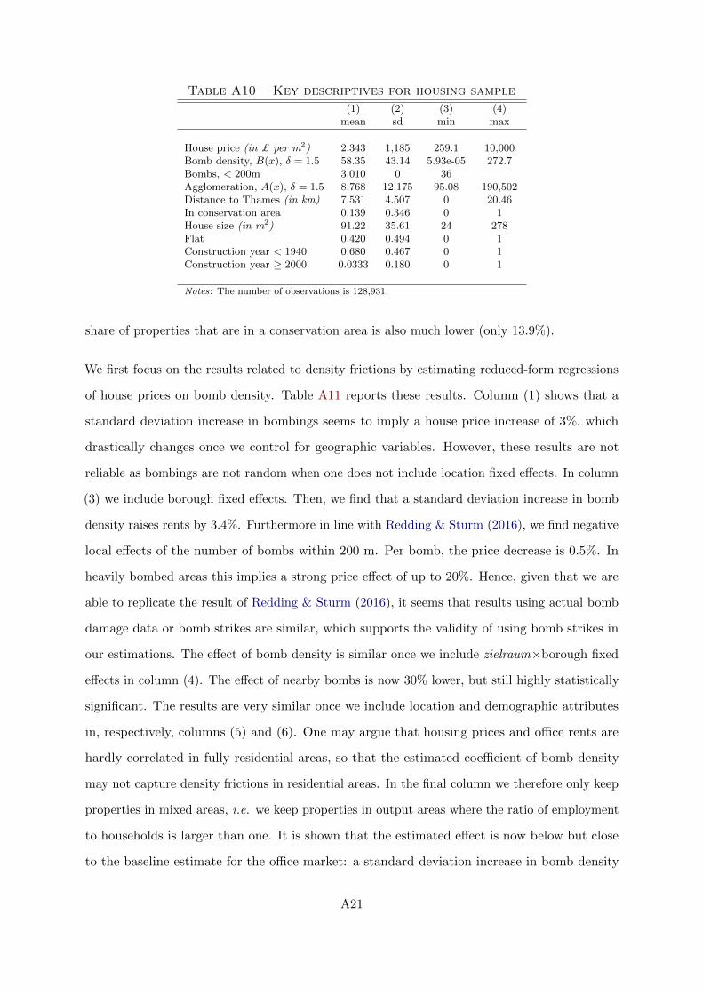
Table A10 – Key descriptives for housing sample

(1) (2) (3) (4)mean sd min max

House price (in £ per m2) 2,343 1,185 259.1 10,000Bomb density, B(x), δ = 1.5 58.35 43.14 5.93e-05 272.7Bombs, < 200m 3.010 0 36Agglomeration, A(x), δ = 1.5 8,768 12,175 95.08 190,502Distance to Thames (in km) 7.531 4.507 0 20.46In conservation area 0.139 0.346 0 1House size (in m2) 91.22 35.61 24 278Flat 0.420 0.494 0 1Construction year < 1940 0.680 0.467 0 1Construction year ≥ 2000 0.0333 0.180 0 1

Notes: The number of observations is 128,931.

share of properties that are in a conservation area is also much lower (only 13.9%).

We first focus on the results related to density frictions by estimating reduced-form regressions

of house prices on bomb density. Table A11 reports these results. Column (1) shows that a

standard deviation increase in bombings seems to imply a house price increase of 3%, which

drastically changes once we control for geographic variables. However, these results are not

reliable as bombings are not random when one does not include location fixed effects. In column

(3) we include borough fixed effects. Then, we find that a standard deviation increase in bomb

density raises rents by 3.4%. Furthermore in line with Redding & Sturm (2016), we find negative

local effects of the number of bombs within 200 m. Per bomb, the price decrease is 0.5%. In

heavily bombed areas this implies a strong price effect of up to 20%. Hence, given that we are

able to replicate the result of Redding & Sturm (2016), it seems that results using actual bomb

damage data or bomb strikes are similar, which supports the validity of using bomb strikes in

our estimations. The effect of bomb density is similar once we include zielraum×borough fixed

effects in column (4). The effect of nearby bombs is now 30% lower, but still highly statistically

significant. The results are very similar once we include location and demographic attributes

in, respectively, columns (5) and (6). One may argue that housing prices and office rents are

hardly correlated in fully residential areas, so that the estimated coefficient of bomb density

may not capture density frictions in residential areas. In the final column we therefore only keep

properties in mixed areas, i.e. we keep properties in output areas where the ratio of employment

to households is larger than one. It is shown that the estimated effect is now below but close

to the baseline estimate for the office market: a standard deviation increase in bomb density

A21

Table A11 – Reduced form results: density frictions and house prices(Dependent variable: the log of house price per m2)

(1) (2) (3) (4) (5) (6) (7)OLS OLS OLS OLS OLS OLS OLS

Bomb density, B(x), δ = 1.5 (std) 0.0304*** -0.0610*** 0.0340*** 0.0297*** 0.0206*** 0.0354*** 0.0616***(0.0019) (0.0019) (0.0025) (0.0030) (0.0029) (0.0026) (0.0057)

Bombs, < 200m 0.0136*** 0.0121*** -0.0054*** -0.0038*** -0.0038*** -0.0029*** -0.0039***(0.0006) (0.0006) (0.0005) (0.0005) (0.0005) (0.0004) (0.0008)

House size (log) -0.3613*** -0.3782*** -0.4157*** -0.4467*** -0.4567*** -0.5104*** -0.4870***(0.0054) (0.0049) (0.0041) (0.0038) (0.0037) (0.0035) (0.0074)

Number of bathrooms 0.0712*** 0.0550*** 0.0414*** 0.0380*** 0.0364*** 0.0308*** 0.0420***(0.0023) (0.0021) (0.0017) (0.0016) (0.0015) (0.0014) (0.0030)

Number of bedrooms 0.0547*** 0.0580*** 0.0610*** 0.0656*** 0.0682*** 0.0727*** 0.0719***(0.0020) (0.0018) (0.0015) (0.0014) (0.0014) (0.0013) (0.0028)

Private parking space -0.0148*** 0.0020 0.0457*** 0.0493*** 0.0473*** 0.0397*** 0.0446***(0.0025) (0.0023) (0.0019) (0.0018) (0.0017) (0.0016) (0.0032)

Garage 0.0549*** 0.0628*** 0.0538*** 0.0500*** 0.0504*** 0.0305*** 0.0213***(0.0026) (0.0024) (0.0020) (0.0019) (0.0018) (0.0017) (0.0036)

House type – detached 0.2468*** 0.2674*** 0.2507*** 0.2317*** 0.2255*** 0.1798*** 0.1672***(0.0048) (0.0046) (0.0041) (0.0039) (0.0038) (0.0035) (0.0081)

House type – semi-detached 0.0818*** 0.0862*** 0.0742*** 0.0648*** 0.0636*** 0.0439*** 0.0403***(0.0027) (0.0025) (0.0020) (0.0019) (0.0019) (0.0016) (0.0036)

House type – flat 0.0837*** 0.0573*** -0.0353*** -0.0607*** -0.0703*** -0.0968*** -0.0831***(0.0033) (0.0030) (0.0024) (0.0022) (0.0022) (0.0020) (0.0041)

House type – maisonette 0.0698*** 0.0439*** -0.0455*** -0.0689*** -0.0765*** -0.1015*** -0.0851***(0.0058) (0.0053) (0.0045) (0.0043) (0.0042) (0.0038) (0.0083)

Constuction year dummies (7) Yes Yes Yes Yes Yes Yes YesYear fixed effects (15) Yes Yes Yes Yes Yes Yes YesGeographical attributes (10) No Yes Yes Yes Yes Yes YesBorough fixed effects (33) No No Yes Yes Yes Yes YesZielraum×borough fixed effects (232) No No No Yes Yes Yes YesLocation attributes (13) No No No No Yes Yes YesDemographic attributes (10) No No No No No Yes Yes

Number of observations 128,931 128,931 128,931 128,931 128,931 128,931 30,307R2 0.7022 0.7497 0.8309 0.8536 0.8592 0.8851 0.8893

Notes: Bomb density is standardised (std) to have mean zero and unit standard deviation. Standard errors are clustered at the postcode and inparentheses; *** p < 0.01, ** p < 0.5, * p < 0.10.

increases house prices by 6.2%.

Second, we focus on the effect of agglomeration economies on house prices of which the second-

stage results are reported in Table A12. The results in the first two columns are again unreliable,

but once we include borough fixed effects we find an elasticity of 0.0732, which is also somewhat

lower than the estimate for the office market. This is confirmed once we include zielraum×borough

fixed effects in column (4) and add location attributes and demographic controls in columns (6)

and (7), respectively. Again, the correlation between house prices and rents is expected to be

higher in mixed areas. Hence, in column (7), we only keep observations in output areas that

have an employment to household ratio of larger than one. The estimated coefficient implies

A22

that doubling agglomeration leads to a house price increase of 12.3%, which is less than half the

estimated elasticity for the office market.

Table A12 – Results: agglomeration economies and house prices(Dependent variable: the log of house price per m2)

(1) (2) (3) (4) (5) (6) (7)2SLS 2SLS 2SLS 2SLS 2SLS 2SLS 2SLS

Agglomeration, A(x), δ = 1.5, (log) 0.0807*** -0.2439*** 0.0732*** 0.0788*** 0.0566*** 0.1024*** 0.1778***(0.0046) (0.0098) (0.0053) (0.0080) (0.0081) (0.0076) (0.0170)

Bombs, < 200m 0.0118*** 0.0162*** -0.0041*** -0.0029*** -0.0032*** -0.0021*** -0.0031***(0.0007) (0.0009) (0.0004) (0.0005) (0.0004) (0.0004) (0.0008)

Constuction year dummies (7) Yes Yes Yes Yes Yes Yes YesYear fixed effects (15) Yes Yes Yes Yes Yes Yes YesGeographical attributes (10) No Yes Yes Yes Yes Yes YesBorough fixed effects (33) No No Yes Yes Yes Yes YesZielraum×borough fixed effects (232) No No No Yes Yes Yes YesLocation attributes (13) No No No No Yes Yes YesDemographic attributes (10) No No No No No Yes Yes

Number of observations 128,931 128,931 128,931 128,931 128,931 128,931 30,307Kleibergen-Paap F -statistic 8,575 4,124 9,544 6,702 6,140 5,943 1,676

Notes: Bold indicates instrumented. Standard errors are clustered at the postcode level and in parentheses; *** p < 0.01, ** p < 0.5, * p < 0.10.

A23

CENTRE FOR ECONOMIC PERFORMANCE Recent Discussion Papers

1541 Andrew B. Bernard Andreas Moxnes

Networks and Trade

1540 Does Gentrification Displace Poor Households? An ‘Identification-Via-Interaction’ Approach

Sevrin Waights

1539 Zhuan Pei Jörn-Steffen Pischke Hannes Schwandt

Poorly Measured Confounders Are More Useful On the Left than On the Right

1538 Konstantin Büchel Stephan Kyburz

Fast Track to Growth? Railway Access, Population Growth and Local Displacement in 19th Century Switzerland

1537 Stephen Gibbons Maria Sánchez-Vidal Olmo Silva

The Bedroom Tax

1536 Pawel Adrjan Brian Bell

Pension Shocks and Wages

1535 Tom Kirchmaier Stephen Machin Matteo Sandi Robert Witt

Prices, Policing and Policy: The Dynamics of Crime Booms and Busts

1534 Laurent Bouton Paola Conconi Francisco Pino Maurizio Zanardi

Guns, Environment and Abortion: How Single-Minded Voters Shape Politicians Decisions

1533 Giulia Giupponi Stephen Machin

Changing the Structure of Minimum Wages: Firm Adjustment and Wage Spillovers

1532 Swati Dhingra Rebecca Freeman Eleonora Mavroeidi

Beyond Tariff Reductions: What Extra Boost From Trade Agreement Provisions?

1531 Doruk Cengiz Arindrajit Dube Attila Lindner Ben Zipperer

The Effect of Minimum Wages on Low-Wage Jobs: Evidence from the United States Using a Bunching Estimator

1530 Stephen Gibbons Vincenzo Scrutinio Shqiponja Telhaj

Teacher Turnover: Does it Matter for Pupil Achievement?

1529 Ghazala Azmat Stefania Simion

Higher Education Funding Reforms: A Comprehensive Analysis of Educational and Labour Market Outcomes in England

1528 Renata Lemos Daniela Scur

All in the Family? CEO Choice and Firm Organization

1527 Stephen Machin Matteo Sandi

Autonomous Schools and Strategic Pupil Exclusion

1526 Stephan E. Maurer Oil Discoveries and Education Spending in the Postbellum South

1525 Paola Conconi Manuel García-Santana Laura Puccio Roberto Venturini

From Final Goods to Inputs: The Protectionist Effect of Rules of Origin

1524 Zack Cooper Fiona Scott Morton Nathan Shekita

Surprise! Out-of-Network Billing for Emergency Care in the United States

The Centre for Economic Performance Publications Unit Tel: +44 (0)20 7955 7673 Email info@cep.lse.ac.uk Website: http://cep.lse.ac.uk Twitter: @CEP_LSE