CERIAS Tech Report 2006-31Beyond k-Anonymity: A Decision Theoretic Framework for Assessing Privacy Risk

by Guy Lebanon, Monica Scannapieco, Mohamed R. Fouad, Elisa BertinoCenter for Education and ResearchInformation Assurance and Security

Purdue University, West Lafayette, IN 47907-2086

1

Beyondk-Anonymity: A Decision TheoreticFramework for Assessing Privacy Risk

Guy Lebanon, Monica Scannapieco, Mohamed R. Fouad, and Elisa Bertino

Abstract

An important issue any organization or individual has to face when managing data containing sensitiveinformation, is the risk that can be incurred when releasingsuch data. Even though data may be sanitized beforebeing released, it is still possible for an adversary to reconstruct the original data using additional information thusresulting in privacy violations. To date, however, a systematic approach to quantify such risks is not available. Inthis paper we develop a framework, based on statistical decision theory, that assesses the relationship between thedisclosed data and the resulting privacy risk. We model the problem of deciding which data to disclose, in termsof deciding which disclosure rule to apply to a database. We assess the privacy risk by taking into account boththe entity identification and the sensitivity of the disclosed information. Furthermore, we prove that, under someconditions, the estimated privacy risk is an upper bound on the true privacy risk. Finally, we relate our frameworkwith the k-anonymity disclosure method. The proposed framework makes the assumptions behindk-anonymityexplicit, quantifies them, and extends them in several natural directions.

I. INTRODUCTION

Data sharing has important advantages in terms of improved services and business, and also for thesociety at large, such as in the case of homeland security. However, unauthorized data disclosures can leadto violations of individuals’ privacy, can result in financial and business damages as in the case of datapertaining to enterprises, or can result in threats to national security as in the case of sensitive geospatialdata.

Preserving the privacy of such data is a complex task driven by two important privacy goals: (i)preventing the identification of the entity relating to the data, and (ii) preventing the disclosure of sensitiveinformation. Entity identification occurs when the released information makes it possible to identify theentity either directly (e.g., by publishing identifiers like SSNs), or indirectly (e.g., by linkage with othersources). Sensitive information includes information that must be protected by law such as medical data,or is deemed sensitive by the entity to whom the data pertains. In the latter case, data sensitivity is asubjective measure whose nature may differ across entities.

In many cases, a careful evaluation needs to be carried out inorder to assess whether the privacyrisk associated with the dissemination of certain data outweighs the benefits of such dissemination. Aspointed out in the recent guidelines issued by the [20], “Some organizations have curtailed access withoutassessing the risk to security, the significance of consequences associated with improper use of the data, orthe public benefits for which the data were originally made available. Contradictory decisions and actionsby different organizations easily negate each organization’s actions.” [19] introduces a way for providingprivacy protection while constructing algorithms that learn information from disparate data and introducesthe notion of privacy-enhanced linking. [5] shows that it isimpossible to achieve privacy with respect toworst-case external knowledge.

To date, however, most of the work related to data privacy hasfocused on how to transform the dataso that no sensitive information is disclosed or linked to specific entities. Because such techniques arebased on data transformations that modify the original datawith the purpose of preserving privacy, the

G. Lebanon is with the Department of Statistics, Purdue University, USA, E-mail: lebanon@stat.purdue.eduM. Scannapieco is with ISTAT, Italy, E-mail: scannapi@istat.itE. Bertino and M. Fouad are with the Department of Computer Science, Purdue University, USA, E-mail:{bertino,mrf}@cs.purdue.edu

2

Organization Database

Disclosed Data

Disclosure Function δ(x)

Linkage Data

Joined

Data

Identified

Dictionary

Fig. 1. Adversarial framework for identity discovery

main focus of such approaches has been the tradeoff between data privacy and data quality e.g., [16], [6].Similar approaches based on output perturbation have been proposed by [2] and [3].

An important practical requirement for any privacy solution is the ability to quantify the privacy risk thatcan be incurred by the release of certain data. Even though data may be sanitized, before being released,it is still possible for an adversary to reconstruct the original data by using additional information thatmay be available, or by record linkage techniques [23]. A possible adversarial scenario is depicted inFigure 1: an attacker exploits data released by an organization by linking it with previously obtained dataconcerning the same entity to gain an enhanced insight aboutthis organization. Indeed, this insight wouldhelp the attacker narrow down possible mismatches when it iscompared against a public dictionary, andconsequently raising the identification risk. The goal of the work presented in this paper is to develop,for the first time, a comprehensive framework for quantifying such privacy risk and supporting informeddisclosure policies.

The framework we propose is based on statistical decision theory and introduces the notion of adisclosure rule that is a function representing the data disclosure policy. Our framework estimates theprivacy risk by taking into account a given disclosure rule and possibly the knowledge that can beexploited by the attacker. It is important to point out that our framework is able to assess privacy risksalso when no information is available concerning the knowledge or dictionary that the adversary mayexploit. The privacy risk function naturally incorporatesboth identity disclosure and sensitive informationdisclosure. We introduce and analyze different shapes of the privacy risk function. Specifically, we definethe risk in the classical decision theory formulation and inthe Bayesian formulation, for either the linkageor the no-linkage scenario. We prove several interesting results within our framework including that underreasonable hypotheses, the estimated privacy risk is an upper bound on the true privacy risk. Finally, wegain insight by showing that the privacy risk is a quantitative framework for exploring the assumptionsand consequences ofk-anonymity.

II. BASICS OFSTATISTICAL DECISION THEORY

Statistical decision theory [21] offers a natural framework for measuring the quantitative effect ofinformation disclosure. As the necessary modifications of decision theory are relatively minor, we areable to adapt a considerable array of tools and results from over 50 years of impressive research. We

3

describe below only the principal concepts of this theory inits traditional abstract setting, and then proceedto apply it to the information disclosure problem.

Statistical decision theory deals with the abstract problem of making decisions in an uncertain situation.Decisions, their properties and the resulting effect are specified formally, enabling their quantitative andrigorous study. The uncertainty is encoded by a parameterθ abstractly called “a state of nature” whichis typically unknown. However, it is known thatθ belongs to a setΘ, usually a finite or infinite subsetof Rl. The decisions are being made based on a sample of observations (x1, . . . , xn), xi ∈ X and arerepresented via a functionδ : X n → A whereA is an abstract action space. The functionδ is referred toas a decision policy or decision rule.

A key element of statistical decision theory is that the state of natureθ governs the distributionpθ(x)that generates the observed data(x1, . . . , xn). Given the state of natureθ, the loss incurred by taking anactionδ(x1, . . . , xn) ∈ A is determined by a non-negative loss function

ℓ : A× Θ → [0, +∞] or ℓ(δ(x1, . . . , xn), θ) ≥ 0.

We sometime denoteℓ(δ(x1, . . . , xn), θ) as δθ(x1, . . . , xn) when we wish to emphasize it as a function,parameterized byθ, of the observed data.

Rather than measuring the loss incurred by a specific decision rule and a specific set of observations,it makes sense to consider the expected loss, or risk, where the expectation is taken over observationsbeing generated from the distribution generating the datapθ. Denoting expectations in general as

Ep(x)(h(x)) =

{∫X

p(x)h(x) dx continuousx∑x∈X p(x)h(x) discretex

the expected loss or risk associated with the decision ruleδ andθ ∈ Θ is

R(δ, θ) = Epθ(x1,...,xn)(ℓ(δ(x1, . . . , xn), θ)) = E∏pθ(xi)(ℓ(δ(x1, . . . , xn), θ))

where the last equality assumes independence ofx1, . . . , xn.The two main statistical paradigms, classical statistics and Bayesian statistics, carry over to decision

theory. In the classical setting of decision theory, the risk R(δ, θ) is the main quantity of interest and itsproperties and relations to different decision rulesδ and statesθ are studied. The Bayesian approach todecision theory assumes that another piece of information is available: our prior beliefs concerning thepossibility of various states of natureθ ∈ Θ. This prior belief is represented by a prior probabilityq(θ)over possible states leading to the Bayes risk

R(δ) = Eq(θ)(R(δ, θ)) = Eq(θ){Epθ(x1,...,xn)(ℓ(δ(x1, . . . , xn), θ))}. (1)

Much has been said in the statistics literature over the controversy between the classical and the Bayesianpoints of view. Without going into this discussion, we simply point out that an advantage of the Bayesrisk is that we can compare different policiesδ1, δ2 based on a single number - their associated risksR(δ1), R(δ2) leading to a partial order on all possible policies. An advantage of the classical frameworkis that there is no need for a prior distributionq - which is often hard or impossible to specify. In bothcases, we need to have a precise specification of the probabilistic modelpθ(x), a set of possible statesof natureΘ and a loss functionℓ. While pθ andΘ depend on modeling assumptions or estimation fromdata, the loss functionℓ is typically elicited from a user and its subjective qualityreflects the personalizednature of risk-based analysis and decision theory.

III. PRIVACY RISK FRAMEWORK

As private information in databases is being disclosed, undesired effects occur such as privacy violations,financial loss due to identity theft, and national security breaches. To proceed with a quantitative formalismwe assume that we obtain a numeric description, referred to as loss, of that undesired effect. The loss may

4

be viewed as a function of two arguments (i) whether the disclosed information enables identification and(ii) the sensitivity of the disclosed information.

The first argument of the loss function encapsulates whetherthe disclosed data can be tied to a specificentity or not. Consider for example the case of a hospital disclosing a list of patients’ gender and whetherthey have a certain medical condition or not. Due to the presence of medical information, such datais clearly sensitive. However, the data sensitivity does not provide any information about the chance oftying the disclosed data to specific individuals and as a result the patients maintain their anonymity andno harmful effect is produced. The clear distinction between data sensitivity and identification, and theircombination via a probabilistic framework, is a central part of our framework. The quantification of theidentification probability depends on (i) the disclosed data, (ii) available side information such as nationalarchives or a phone-book, and (iii) an attacker model.

In contrast to the identification probability, the second argument of the loss function concerning the datasensitivity depends on the entity associated with the data.Data such as annual income, medical history,internet purchases etc. relating to specific users may be very sensitive to some but only marginally sensitiveto others. Such personalized or customized sensitivity measures are important to take into considerationwhen measuring harmful effects and deciding on a disclosurepolicy. Clearly, ignoring it may lead tooffering insufficient protection to a subset of people whileapplying excessive protection to the privacy ofanother subset. It is worth pointing out that we do not draw a distinction between sensitive attributes andquasi-identifiers [13], [24], [12]. Rather, our framework provides more flexibility by enabling the ownersof the data to supply the sensitivity of their attributes at their discretion.

We assume that the data resides in a relational database withthe relational scheme(A1, . . . , Am), whereeach attributeAi takes values in a domain Domi which includes a possible missing value symbol⊥. Thespace

X = Dom1 × Dom2 × · · · × Domm

represents the set of all possible records, both original records residing in a database and disclosed records.We make the following assumption for the sake of notational simplicity, none of which are crucial to thepresented framework. First, we assume that one of the attributesA1 uniquely identifies the entity associatedwith the record. This attribute will typically not be disclosed, but is important for notational convenience.Second, we assume that the symbol⊥ ∈ Domi for all i, corresponds to both a missing value in thedatabase and to attribute values that are suppressed duringthe disclosure procedure. Suppression of the(non-missing)j-attribute in a recordy ∈ X may thus be represented by a functionδ : X → X for which[δ(y)]j = ⊥. Finally, we assume that the spaceX is sufficiently rich to denote attribute generalizations,for example

North America ∈ Domcountry

represents a generalization of the country attribute to a more vague concept.We will usually refer to an arbitrary record asx, y or z and to a specific record in a particular database

using a subscriptxi (note the bold-italic typesetting representing vector notation). The attribute valuesof records are represented using the notation[x]j , [xi]j or just xj or xij respectively (note the non-boldtypesetting). A collection ofn records, for example a database containingn records, is represented by(x1, . . . , xn) ⊆ X n.

A. Disclosure Rules and Privacy Risk

Adapting the decision theory framework described in the previous section to privacy requires relativelyfew changes. Instead of decision policiesδ : X n → A we have disclosure policiesδ : X → X representingdisclosing the data as isδ(z) = z, attribute suppression (e.g.,[δ(z)]j = ⊥), or attribute generalization(e.g., [δ(z)]j = North America).

The state of natureθ that influences the incurred lossℓθ = ℓ(·, θ) is the side information used by theattacker in their identification attempt. Such side information θ is often a public data resource composed

5

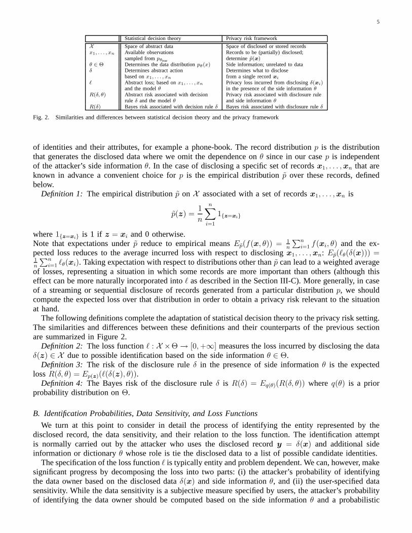
Statistical decision theory Privacy risk framework

X Space of abstract data Space of disclosed or stored recordsx1, . . . , xn Available observations Records to be (partially) disclosed;

sampled frompθtrue determinep(x)θ ∈ Θ Determines the data distributionpθ(x) Side information; unrelated to dataδ Determines abstract action Determines what to disclose

based onx1, . . . , xn from a single recordxi

ℓ Abstract loss; based onx1, . . . , xn Privacy loss incurred from disclosingδ(xi)and the modelθ in the presence of the side informationθ

R(δ, θ) Abstract risk associated with decision Privacy risk associated with disclosure rulerule δ and the modelθ and side informationθ

R(δ) Bayes risk associated with decision ruleδ Bayes risk associated with disclosure ruleδ

Fig. 2. Similarities and differences between statistical decision theory and the privacy framework

of identities and their attributes, for example a phone-book. The record distributionp is the distributionthat generates the disclosed data where we omit the dependence onθ since in our casep is independentof the attacker’s side informationθ. In the case of disclosing a specific set of recordsx1, . . . , xn that areknown in advance a convenient choice forp is the empirical distributionp over these records, definedbelow.

Definition 1: The empirical distributionp on X associated with a set of recordsx1, . . . , xn is

p(z) =1

n

n∑

i=1

1{z=xi}

where1{z=xi} is 1 if z = xi and 0 otherwise.Note that expectations underp reduce to empirical meansEp(f(x, θ)) = 1

n

∑ni=1 f(xi, θ) and the ex-

pected loss reduces to the average incurred loss with respect to disclosingx1, . . . , xn: Ep(ℓθ(δ(x))) =1n

∑ni=1 ℓθ(xi). Taking expectation with respect to distributions other than p can lead to a weighted average

of losses, representing a situation in which some records are more important than others (although thiseffect can be more naturally incorporated intoℓ as described in the Section III-C). More generally, in caseof a streaming or sequential disclosure of records generated from a particular distributionp, we shouldcompute the expected loss over that distribution in order toobtain a privacy risk relevant to the situationat hand.

The following definitions complete the adaptation of statistical decision theory to the privacy risk setting.The similarities and differences between these definitionsand their counterparts of the previous sectionare summarized in Figure 2.

Definition 2: The loss functionℓ : X ×Θ → [0, +∞] measures the loss incurred by disclosing the dataδ(z) ∈ X due to possible identification based on the side informationθ ∈ Θ.

Definition 3: The risk of the disclosure ruleδ in the presence of side informationθ is the expectedlossR(δ, θ) = Ep(z)(ℓ(δ(z), θ)).

Definition 4: The Bayes risk of the disclosure ruleδ is R(δ) = Eq(θ)(R(δ, θ)) whereq(θ) is a priorprobability distribution onΘ.

B. Identification Probabilities, Data Sensitivity, and Loss Functions

We turn at this point to consider in detail the process of identifying the entity represented by thedisclosed record, the data sensitivity, and their relationto the loss function. The identification attemptis normally carried out by the attacker who uses the disclosed recordy = δ(x) and additional sideinformation or dictionaryθ whose role is tie the disclosed data to a list of possible candidate identities.

The specification of the loss functionℓ is typically entity and problem dependent. We can, however,makesignificant progress by decomposing the loss into two parts:(i) the attacker’s probability of identifyingthe data owner based on the disclosed dataδ(x) and side informationθ, and (ii) the user-specified datasensitivity. While the data sensitivity is a subjective measure specified by users, the attacker’s probabilityof identifying the data owner should be computed based on theside informationθ and a probabilistic

6

attacker model. We proceed below with describing a reasonable derivation of the attacker’s identificationprobability and then proceed with a description of the user-specified data sensitivity function.

Given a disclosed recordδ(x), and available side information or dictionaryθ the attacker can narrowdown the list of possible identities to the subset of entity entries inθ that are consistent with the disclosedattributesδ(x). For example, considerx being(first-name, surname, phone-number) andthe dictionaryθ being a phone-book. The attacker needs only to consider dictionary entities that areconsistent with the disclosed recordδ(x). For example, if there are no missing values and the entire recordis disclosed i.e.,δ(x) = x, it is likely that only one entity exists in the dictionary that is consistent withthe disclosed information. On the other hand, if the attribute value forphone-number is suppressed,the phone-bookθ may yield more than a single consistent entity, depending onthe popularity of thecombination (first-name, surname).

Formalizing the above idea we define the binary random variable Z which equals 1 if the attackersuccessfully identified the data owner and 0 otherwise. The identification probabilityp(Z = 1) dependson the attacker, but in the absence of additional information we may assume that the identification attemptis a uniform selection from the set of entities inθ consistent with the disclosedδ(x), denoted byρ(δ(x), θ),

p(Z = 1) =

{|ρ(δ(x), θ)|−1 if ρ(δ(x), θ) 6= ∅

0 if ρ(δ(x), θ) = ∅and p(Z = 0) = 1 − p(Z = 1).

The data sensitivity is determined by two user specified functions Φ, Ψ : X → [0, +∞]. Φ measuresthe harmful effect of disclosing the data assuming that the attacker’s identification is successful i.e.Φ(x) = ℓ(δ(x), θ) | {Z = 1}. Similarly, Ψ measures the harmful effect of disclosing the data assumingthat the attacker’s identification was unsuccessful i.e.Ψ(x) = ℓ(δ(x), θ) | {Z = 0}.

Putting the identification probability and sensitivity function together, we have that the harmful effectis a random variable with two possible outcomes:Φ(δ(x)) with probability p(Z = 1) andΨ(δ(x)) withprobability p(Z = 0). Accounting for the uncertainty resulting from possible identification we define thelossℓ(y, θ) as the expectation

ℓ(δ(x), θ) = p(Z = 1) · Φ(δ(x)) + p(Z = 0)Ψ(δ(x)).

Allowing Φ, Ψ to take on the value+∞ enables us to model situations where the data sensitivity issohigh that its disclosure is categorically prohibited (ifΨ(δ(x)) = +∞) of is prohibited under any positiveidentification chance (ifΦ(δ(x)) = +∞).

It is often the case that no harmful effect is caused if the attacker’s identification attempt fails leadingto Ψ ≡ 0. For simplicity, we assume this is the case in the remainder of the paper, leading toℓ(δ(x), θ) =p(Z = 1)Φ(δ(x)). The riskR(δ, θ) with respect to the empirical distributionp over the disclosed recordsis

R(δ, θ) = Ep(ℓ(δ(z), θ)) =1

n

∑

i : ρ(δ(xi),θ)6=∅

Φ(δ(xi))

|ρ(δ(xi), θ)|

and the Bayes risk under the priorq(θ) is

R(δ) = Ep(R(δ, θ)) =1

n

n∑

i=1

Φ(δ(xi))

∫

Θ

1{ρ(δ(xi),θ)6=∅}q(θ)

|ρ(δ(xi), θ)|dθ

or its discrete equivalent ifΘ is a discrete space. Similar expressions can be computed if the assumptionΨ ≡ 0 is relaxed.

7

C. Parametric Families of Sensitivity Functions

We now present several possible families of expressions forthe data sensitivity functionΦ. SinceΦ isdefined on the setX of all possible records, defining it by a lookup table is impractical for a large numberof attributes. We therefore consider several options leading to compact and efficient representations. Givena disclosed recordy = δ(x), perhaps the simplest meaningful form forΦ is a linear combination of non-negative weightswj ≥ 0 over the disclosed attributes

Φ1(y) =∑

j : yj 6=⊥

wj (2)

where wj represents the sensitivity associated with the corresponding attributeAj . A weight of +∞represents critically sensitive information that may onlybe disclosed if there is zero chance of it leadingto identification.

In some cases, the data sensitivity significantly depends onthe entity associated with the record. In otherwords attributesAi may be highly sensitive for some records and less so for otherrecords. Recalling theassumption that one of the attributes, sayy1, represents a unique identifier, we can construct the followingpersonalized linear sensitivity function

Φ2(y) =∑

j:yj 6=⊥

wj,y1. (3)

The weights{wj,r : j = 1, . . . , n} should be elicited from the different entities corresponding to the recordsor otherwise assigned by the database according to the groupor cluster they belong to. Normalizationconstraints such as

∀r∑

j

wj,r = c or ∀r∑

j

wj,r ≤ c

can be enforced to provide all entities with similar privacyprotection, or to make sure that no singleentity dominates the privacy risk.

There are a number of ways to increase the flexibility of sensitivity functions beyond linear forms. Oneway to do so is by forming linear expressions containingk-order interaction terms, e.g., fork = 2

Φ3(y) =∑

j>1:yj 6=⊥

wj,y1+

∑

j>1:yj 6=⊥

∑

h>j:yh 6=⊥

wj,h,y1. (4)

Expressions containingk-order interaction terms use additional weights to captureinteractions of at mostk attributes that are not accounted for in the expressions (2)-(3). As k increases in magnitude, the classof functions represented byΦ becomes richer and in the case ofk = m provides arbitrary flexibility.However, increasingk beyond a certain limit is impractical as both the number of weights specified bythe users as well as the computational complexity associated with Φ4 grow exponentially withk.

A possible alternative to the linear sensitivity function is a multiplicative function

Φ4(y) = exp

∑

j:yj 6=⊥

wj,y1

=∏

j:yj 6=⊥

ewj,y1 (5)

in which case increasing one weightwi,j while fixing the others causes the sensitivity to increaseexponentially in contrast to (2)-(4). The precise choice ofthe sensitivity functionΦ (andΨ is applicable)ultimately depends on the database policy and entities relating to the data. A simple such as (3) or (5)has the advantage of being easier to elicit and interpret.

8

Midwest

Indiana

Indianapolis Tippecanoe

Greater Lafayette

West Lafayette

Lafayette

Illinois

Battle Ground Buck Creek Clarks Hill Dayton Romney

Fig. 3. A partial value generalization hierarchy (VGH) for the address field

D. Data Suppression and Generalization and the Privacy Risk

A common practice in privacy preservation is to replace datarecords with suppressed or more generalvalues [16], [17] in order to ensure anonymity and prevent the disclosure of sensitive data. A disclosurepolicy δ : X → X can suppress an attribute by assigning a⊥ symbol to the appropriate attribute i.e.[δ(x)]j = ⊥.

Assuming that the spaceX is rich enough to contain the necessary generalizations, attribute valuegeneralization may be accomplished by assigning a disclosed value that is more general than the originalattribute valuexj ≺ [δ(x)]j . Formally, we assume that Domi is a partially ordered set(Si,≺) whosesmallest elements correspond to non-generalized attribute values and whose single maximum element isthe ultimate generalized value, which we identify with the suppressed or missing value introduced earlier⊥.

The partially ordered set Domi may be illustrated using its Hasse diagram in which every nodecorrespond to a member of Domi and the edges correspond to the covering relation:x covers y ify ≺ x and ∄z : y ≺ z ≺ x [18]. Furthermore when drawing the Hasse diagram we draw more generalnodes vertically higher than less general nodes. As an example, consider the attribute value representinga location or address and several levels of generalized values. A partial Hasse diagram representing thepartial value generalization hierarchy for this attributeis illustrated in Figure 3. In this particular case,the Hasse diagram is relatively simple and is graphically described using a tree structure. More generalexamples and properties of partially ordered set may be found in [18].

Replacing an attribute valuexj by a more general valuexj i.e. xj ≺ xj increases the set of entitiesconsistent with that value in the attacker’s dictionaryθ i.e.

xj � xj =⇒ ρ((x1, . . . , xj, . . . , xm), θ) ⊆ ρ((x1, . . . , xj , . . . , xm), θ) (6)

where ρ(x, θ) is the set of entities inθ consistent withx. Equation (6) indicates that as expected,generalizing an attribute value (which includes suppression as a special case) reduces the identificationprobability p(Z = 1).

Equation (6) together with the assumption that the data sensitivity function Φ assigns smaller valuesto more general data ensures that the lossℓ(δ(x), θ) decreases with the amount of data generalization.The precise constraint onΦ depends on its parametric form e.g. (2)-(5). For example, inthe case of apersonalized linear sensitivity (3) the appropriate constraints on the weights are

1) wa ≥ 02) wa,r ≤ wb,r ∀a � b ∀r.

9

U(δ)

R(δ, θ)

Fig. 4. Space of disclosure rules and their risk and expectedutility. The shaded region correspond to all achievable disclosure policiesδ.

3) w⊥ = 0.The last constraint above is not crucial, but it ensures thatfully suppressed data have zero sensitivityΦ(⊥, . . . ,⊥) = 0.

In summary, as we generalize or suppress data both the identification probabilityp(Z = 1) and datasensitivity Φ(δ(x)) decrease leading to lower lossℓ(δ(x, θ)) and lower riskR(δ, θ). Considering thedisclosure riskR(δ, θ) by itself leads to the conclusion that in order to minimize the risk the data needsto be completely suppressed or generalized. However, such aconclusion misses the point since it ignoresthe benefit obtained from the data disclosure. In order to appropriately appreciate the trade-off betweenthe risk and benefit associated with private data disclosurewe extend our discussion in the next sectionto include a quantification of the benefit associated with data disclosure.

IV. THE OPTIMAL DISCLOSUREPOLICIES

Apart from incurring a privacy risk, disclosing private data δ(x) has some benefit, or else data wouldnever be disclosed. We represent this benefit by a utility function u : X → R+ whose expectation

U(δ) = Ep(x)(u(δ(x)))

plays a similar but opposing role to the riskR(δ, θ). While the lossℓ(δ(x), θ) is user specified andmay change from user to user, the utility is typically specified by the disclosing organization or the datarecipient and is not user dependent.

The relationship between the risk and expected utility is schematically depicted in Figure 4 whichdisplays disclosure policiesδ by their 2-D coordinates(R, U) representing their risk and expected utility.The shaded region in the figure correspond to the set of achievable disclosure policies i.e. every coordinate(R, U) in that region correspond to one or more policiesδ realizing it. The unshaded region correspondto un-achievable policies i.e. there does not exist anyδ with the corresponding risk and expected utility.The vertical line in the figure correspond to all rules whose risk is fixed at a certain level. Similarly,the horizontal line correspond to all rules whose expected utility is fixed at a certain level. Since thedisclosure goal is obtain both low risk and high expected utility, we are naturally most interested indisclosure policies occupying the boundary or frontier of the shaded region. Policies in the interior of theshaded region can be improved upon by projecting them to the boundary.

The vertical and horizontal lines suggest the following twoways of resolving the risk-utility tradeoff.Assuming that we cannot afford incurring risk higher than some acceptable level we can define the optimalpolicy as

δ∗ = arg maxδ

U(δ) subject to R(δ, θ) ≤ c. (7)

10

Alternatively, insisting on having expected utility no less than a certain acceptable level we can definethe optimal policy to be

δ∗ = arg minδ

R(δ, θ) subject to U(δ) ≥ c. (8)

A more symmetric definition of optimality is given by

δ∗ = arg minδ

R(δ, θ) − λU(δ) (9)

where λ ∈ R+ is a parameter controlling the relative importance of minimizing risk and maximizingutility.

The formation and interpretation of optimality depends on the situation at hand and is ultimately up topolicy makers. We focus below on the case (8), but to simplifythe notation we denote∆ = {δ : U(δ) ≥ c}so that (8) becomesδ∗ = arg minδ∈∆ R(δ, θ). Solving (8) may often be computationally challengingas it is not easy to get a closed form definition of the constraint set ∆ = {δ : U(δ) ≥ c}. Moreefficient computational search can usually be obtained by considering insteadδ∗ = arg minδ∈∆ R(δ)

where∆ = {δ : ∀i, u(δ(xi)) ≥ c} ⊆ ∆.Solving the optimization problems (7)-(9) requires knowledge of the attacker’s side informationθ.

Indeed, in some cases the attacker’s side information is known - for example whenθ constitutes nationalarchives or some other publicly available dataset. In caseswhere the attacker’s side informationθ isunknown we can proceed instead using one of the following approaches.

• Bayes Risk ReplacingR(δ, θ) in (7)-(9) with the Bayes riskR(δ) = Eq(θ)(R(δ, θ)) provides Bayesian-optimal policies that are independent ofθ .

• Estimating θ In some cases we can obtain an estimate of the attacker’s sideinformation θ. In thesecases we can use expressions (7)-(9) withR(δ, θ) replaced byR(δ, θ). Mathematical analysis canbe used to study the quality of the approximationR(δ, θ) ≈ R(δ, θ) in terms of the approximationθ ≈ θ.

• Worst Case Scenario In the absence of any information concerningθ we can use (7)-(9) with theworst case riskmaxθ∈Θ R(δ, θ) instead ofR(δ, θ). The resulting policies, for example the minimaxrisk δ∗ = arg minδ∈∆ maxθ∈Θ R(δ, θ), have the best worst case scenario.

• Bounding the Risk This approach is described in the next Section.

A. Bounding the True Risk by the Estimated Risk

As mentioned above, we can use an estimateθ instead of theθtrue and estimate the risk byR(δ, θ). Insome cases, as described below we can bound the true risk in terms of the estimated riskR(δ, θtrue) ≤R(δ, θ) as well as the risk of the optimal policyarg minδ∈∆ R(δ, θtrue) ≤ arg minδ∈∆ R(δ, θ).

A frequent situation is when the estimateθ is obtained from the organization’s records while the at-tacker’s dictionaryθtrue is a more general-purpose dictionary. In other words, the estimated side informationθ is more specific than the attacker’s dictionary. For example, sinceθtrue is more general, it contains therecords inθ as well as additional records. Following the same reasoningwe can also assume that for eachrecord that exists in both dictionaries,θtrue will have more general attribute values thanθ.

For example, consider a database of employee records for some company.θ would be a dictionaryconstructed from the database andθtrue would be a general-purpose dictionary available to the attacker. Itis natural to assume thatθtrue will contain additional records over the records inθ and that the attributesin θtrue (e.g.,first-name,surname,phone#) will be more general than the attributes inθ. After all, someof the record attributes are private and would not be disclosed in order to find their way into the attacker’sdictionary (resulting in more⊥ symbols inθtrue).

Below, we consider dictionariesθ = (θ1, . . . , θl) as relational tables, whereθi = (θi1, . . . , θiq) is arecord of a relationTθ(A1, . . . , Aq), with A1 corresponding to the record identifier.

11

Definition 5: We define a partial order relation≪ between dictionariesθ = (θ1, . . . , θl1) and η =(η1, . . . , ηl2) by saying thatθ ≪ η if for every θi, ∃ηj such thatηj1 = θi1 and∀k θik � ηjk.

Theorem 1:If θ contains records that correspond tox1, . . . , xn and θ ≪ θtrue, then

∀δ R(δ, θtrue) ≤ R(δ, θ).Proof: For every disclosed recordδ(xi) there exists a record inθ that corresponds to it and since

θ ≪ θtrue there is also a record inθtrue that corresponds to it. As a result,ρ(δ(xi), θ) and ρ(δ(xi), θtrue)

are non-empty sets.For an arbitrarya ∈ ρ(δ(xi), θ) we havea = θv for somev and sinceθ ≪ θtrue there exists a

corresponding recordθtruek . The recordθtrue

k will have the same (or more) general values asa and thereforeθtrue

k ∈ ρ(δ(xi), θtrue). The same argument can be repeated for everya ∈ ρ(δ(xi), θ) thus showing that

ρ(δ(xi), θ) ⊆ ρ(δ(xi), θtrue) or |ρ(δ(xi), θ

true)|−1 ≤ |ρ(δ(xi), θ)|−1.

The probability of identifyingδ(xi) by the attacker is thus smaller than the identification probabilitybased onθ and it follows that

∀i ℓ(δ(xi), θtrue) ≤ ℓ(δ(xi), θ) ⇒ R(δ, θtrue) ≤ R(δ, θ).

B. Independence and Integrity Constraints

Computing and minimizing the risk may be computationally demanding in the general case. In thissection we discuss how the independence assumption or its relaxation by introducing integrity constraintsaffect such computational efficiency considerations.

The assumption that different attributes are statistically independent is somewhat questionable but stilloften used in high dimensions due to its practicality. For instance, returning to the simple phone-bookexample, the independence assumption may imply that the popularity of first names does not depend onthe popularity of last names, e.g.,

p(first-name= Mary|surname= Smith) = p(first-name= Mary|surname= Johnson)

= p(first-name= Mary).

Clearly, some attributes are strongly correlated while others are generally believed to be independent. Theintroduction of integrity constraints to model correlatedattributes (e.g., profession =A ⇒ salary∈ C)while assuming independence between uncorrelated attributes is an effective relaxation of the completeindependence assumption. We first discuss the implication of complete independence to risk computationand then proceed to consider the presence of integrity constraints.

Under the assumption of statistical independence on the database attributes the identification distributionfactors as a product

|ρ(δ(xi), θ)|

N=

∏

j

|ρj([δ(xi)]j, θ)|

N⇒ |ρ(δ(xi), θ)| =

∏

j

αj([δ(xi)]j , θ)

for some appropriate functionsαj . As a result the loss function (assuming a parametric multiplicativeform) decomposes to

ℓ(y, θ) =

∏j∈C2(y) ewj,y1

|ρ(y, θ)|=

∏j∈C2(y) ewj,y1

∏k>1 αk(yk, θ)

=∏

j∈C2(y)

ewj,y1

αj(yj, θ)·

∏

l∈C1(y)

1

αl(⊥, θ)

=∏

j∈C2(y)

ewj,y1

αj(⊥, θ)

αj(yj, θ)·

m∏

l=2

1

αl(⊥, θ).

whereC1(y) = {j : j > 1, yj = ⊥} andC2(y) = {j : j > 1, yj 6= ⊥}.

12

To select the disclosure ofk attributes that minimizes the above loss it remains to select the setC2(y)

of k indices that minimizes the loss. This set corresponds to thek smallest elements of{ewj,y1αj(⊥,θ)

αj(yj ,θ)}m

j=2

which may be efficiently computed in timeO(nNm) wheren, N, m are the number of disclosed records,dictionary size, and number of attributes [11].

Extensions of the above decomposition are straightforwardwhen the attributes can be divided to severalclusters satisfying statistical dependence for attributes within the same cluster and statistical independencefor attributes belonging to different clusters. An alternative decomposition for more general integrityconstraints or dependencies may be obtained through the product factorization of graphical models instatistics [22].

V. PRIVACY RISK AND k-ANONYMITY

k-Anonymity [16] has recently received considerable attention by the research community [25], [1].Given a relationT , k-anonymity ensures that each disclosed record can be indistinctly matched to at leastk individuals in T . It is enforced by considering a subset of the attributes called quasi-identifiers, andforcing the disclosed values of these attributes to appear at leastk times in the database.k-Anonymityuses two operators to accomplish this task: suppression andgeneralization.

In its original formulation,k-anonymity does not seem to make any assumptions on the possible externalknowledge that could be used for entity identification and does not refer to a privacy loss. However,k-anonymity does make strong implicit assumptions whose presence may undermine its original motivation.Following the formal presentation ofk-anonymity in the privacy risk context, we analyze these assumptionsand their possible relaxations.

Since thek-anonymity requirement is enforced on the relationT , the anonymization algorithm considersthe attacker’s side informationθtrue as equal to the relation or databaseT . Representing thek-anonymityrule by δ∗k we have that thek-anonymity constraints may be written as

∀i |ρ(δ∗k(xi), T )| ≥ k. (10)

The sensitivity function is taken to be constantΦ ≡ c ask-anonymity is concerned with only satisfyingthe constraints (10). In fact it treats disclosure of different attributes corresponding to different entities asequal, as long as the constraints (10) hold.

As a result, the loss incurred byk-anonymity δ∗k is bounded byℓ(δ∗k(xi), T ) ≤ c/k where equalityis achieved if the constraint|ρ(δ∗k(xi), T )| = k is met. On the other hand, any ruleδ0 that violatesthe k-anonymity requirement for somexi will incur a loss higher (underθ = T and Φ ≡ c) than thek-anonymity rule

ℓ(δ0(xi), T ) =c

|ρ(δ0(xi), T )|≥ ℓ(δ∗k(xi), T ).

We thus have the following result presentingk-anonymity as optimal in terms of the privacy risk frame-work.

Theorem 2:Let δ∗k be ak-anonymity rule andδ0 be a rule that violates thek-anonymity constraint,both with respect toxi ∈ T . Then

ℓ(δ∗k(xi), T ) ≤ c/k < ℓ(δ0(xi), T ).As the above theorem implies, thek-anonymity rule minimizes the privacy loss per examplexi and

may be seen asarg minδ∈∆ R(δ, T ) where∆ is a set of rules that includes bothk-anonymity rules andrules that violate thek-anonymity constraints. The assumptions underlyingk-anonymity, in terms of theprivacy risk framework are:

1) θtrue = T ,2) Φ ≡ c, and3) ∆ is under-specified.

13

The first assumption may be taken as an indication thatk-anonymity simply assumes that the databaserelationT is available as side information to the attacker. This assumption can be expanded as describedearlier by assuming an estimatedθ, using a Bayesian averaging, worst case riskmaxθ∈Θ R(δ, θ) or thatθtrue is a publicly available resource. Such adaptation ofk-anonymity are likely to more faithfully protectprivacy and yet should not require a major conceptual changeto thek-anonymity framework.

The second assumption of the sensitivity functionΦ ≡ c being constant is a result ofk-anonymity’ssingular attention to protection from identification. In other words, disclosing data incurs the same lossregardless of the data itself and the entity to whom the data pertains, as long as there exists a certainprotection from identification. This is a problematic assumption since under imperfect identification protec-tion, the notion of privacy preservation is not not synonymous with identification. Imperfect identificationprotection occurs since a positive probability of identification remains, whether by the original data’sdisclosure or by linkage as described in the next section. Asa result, it is imperative to take intoconsideration also the sensitivity of the disclosed information.

As a simple example, consider facing two possible disclosure options: the disclosure of data containinga substantial medical diagnosis (e.g., HIV positive) and the disclosure of data containing a recent groceryshopping transaction. Intuitively, disclosing the first data would lead to a greater privacy violation than thesecond data under non-zero identification probability. Howeverk-anonymity, assuming a constant sensi-tivity function, considers the disclosure of both data equally harmful if they provide similar identificationprotection. On the other hand, it may favor the disclosure ofvery sensitive information if it providesslightly better identification protection than relativelynon-sensitive data. Section VIII presents a casestudy illustrating this point further in the context of a commercial organization’s customer transactiondatabase. For a diverse commercial organization such as Amazon.com transactions should be classifiedaccording to varying sensitivity levels.k-Anonymity protection would exert undesired privacy protectionin some areas while lacking in other areas. The privacy risk framework presented in this paper providesa natural extension tok-anonymity by makingΦ non-constant. The resulting privacy loss combines datasensitivity and identification protection in quantitativeprobabilistic manner.

The third assumption implies that the set∆ may be specified in several ways. Recall that the riskminimization framework is based on the assumption that there is a tradeoff in disclosing private informa-tion. On one hand the disclosed data incurs a privacy loss andon the other hand disclosing data servessome benefit. The risk minimization frameworkarg minδ∈∆ R(δ, θ) assumes that∆ contains a set of rulesacceptable in terms of their disclosure benefit, and from which we select the one incurring the least risk.k-Anonymity ignores this tradeoff and the set of candidate rules ∆ may be specified in several ways, forexample∆ = ∆0 ∪ {δ∗k} where∆0 contains rules that violate thek-anonymity constraints.

VI. PRIVACY RISK AND RECORD L INKAGE

We have thus far discussed the usage of a dictionary to identify the entity associated with a disclosedrecord. Sometimes, side information is used in a different way to link disclosed records with additionaldata. The linkage, if successful, enlarges the available information thereby influencing both the datasensitivity and subsequent identification probability. The probabilistic framework of the privacy risk canbe naturally extended to account for such cases. Figure 1 illustrates the linkage process in the context ofthe privacy risk framework.

We say that the linkage of the disclosed dataδ(x) and public recordz is successful ifδ(x) andz arerecords that relate to the same entity [7]. The linkage ofδ(xi) andz creates an enlarged set of attributesδ(xi) ∨ z combining information from both sources, which if successful, improves identification basedon a dictionary. Note that while both linkage data and the dictionary are side information known to theattacker, they serve different roles. Linkage data typically comes from the organization that disclosesδ(xi) or a related database. In particular, it does not typically contain identification information and yetis used by the attacker in order to extend the disclosed attributes of a certain entity. The dictionary istypically a massive listing containing identification information that is not closely related to the disclosed

14

information. It is therefore considered as an identification resource for the disclosed and possibly linkedrecord.

The disclosed recordy = δ(x) and the linked recordz are random variables with a joint distributionp(x, z) = p(x)p(z|y) wherep(x) may be the empiricalp(x) described earlier and the conditionalp(z|y)is the probability of linking recordz with recordy. In this case, it is important to estimate the linkingprobability based on what a sensible attacker might do. In the case of linkingδ(xi) ∨ z, the risk is

Rlink(δ, θ) = Ep(x)p(z|x)(ℓ(δ(x) ∨ z, θ))

where the loss functionℓ(δ(xi) ∨ z) can be structured in a similar way to our previous discussion.Introducing a binary random variableW representing successful linking we have that the loss incurredunder successful linking and identification is equal to the sensitivity of the enlarged data

Φ(δ(x) ∨ z, θ) = ℓ(δ(x) ∨ z, θ)) | {W = 1, Z = 1}.

Continuing as before, we can define the lossℓ(δ(x) ∨ z, θ) as the expectation of the sensitivity takinginto consideration probabilities of successful linking and identification. As before, it is crucial that thedeveloped mechanism lead to easy and accurate calculation of the loss.

VII. A PPLICATIONS AND EXPERIMENTS

In this section, we define two operators that implement disclosure rules on relations (Section VII-A),and then proceed to illustrate some experiments further validating our framework (Section VII-B).

A. Implementation of Disclosure Rules

As described in Section III-D, disclosure rules can lead to data generalization or even to data suppression.In this section we describe two operators that implement disclosure rules in a relational setting. Inparticular, we show that we can define such operators by relying on relational algebra, thus enablingthe usage of relational technology. The definition in relational algebra allows us to prove some interestingproperties as well as to obtain consistent advantages in terms of standardization and efficiency of thedisclosure rules implementation. More specifically, the algebraic specification of the operators paves theway for the realization of optimization strategies within relational technology.

Consider the relationT (A1, . . . , Am), and the setX = Dom1 × · · · × Domm. Recall that the attributeA1 is supposed to be a record identifier for the relationT . Let F be a formula involving: (i) a set ofoperands that are either variables or constants, (ii) the set of arithmetic operators{=, 6=, <,≤, >,≥}, and(iii) the set of logical operators{∨,∧,¬}. Such formulas are used to specifydisclosure conditions, i.e.to identify the tuples of a relation which are subject to privacy constraints and on which disclosure rulesmust be enforced.

We first define the operatorhideT that enables attribute-level suppression on the tableT .Definition 6: Given an attributeAj of the relationT , and a formula F, the operatorhideT is defined as

hideT (Aj, F ) = (Π〈A1,Aj〉σF T ) ⊲⊳=A1T

First, the operator selects the tuples satisfying the condition F in the relationT . The selectionσF

specifies which tuples donot have privacy requirements on the attributeAj. Second, the projectionΠ〈A1,Aj〉

builds a partial result used to recompose the original relation, with ⊥ values replacing the values ofAj tobe kept private. For this latter step, the right outer join operator⊲⊳= is applied over the record identifierA1, and is used to introduce the⊥ values wherever specified by the disclosure conditions. Note that theouter join operator is used in cases when it is required that the resulting relation contains all tuples fromboth relations, even if they do not participate in the join. In such cases they are padded with⊥ values[15].

The following proposition formally states the commutativeand associative properties of the operator,that are directly derived from properties of relational algebra.

15

A1 A2 A3 A4

1 a1 b1 c12 a2 b2 c23 a3 b3 c3

⇒A1 A2

2 a2

The starting relationT T ∗ = Π〈A1,A2〉σA1 6=1∧A1 6=3T⇓

A1 A2 A3 A4

1 ⊥ b1 c12 a2 b2 c23 ⊥ b3 c3

The target relationT ′ = T ∗ ⊲⊳=A1T

Fig. 5. ThehideT (A2, F′ ∧ F ′′) operator

A1 A2 A3 A4

1 a1 b1 c12 a2 b2 c23 a3 b3 c3

A1 A2

1 a1

2 a2

3 a3

The starting relationT The generalized relationGF

⇓

A1 A2 A3 A4 A2

1 a1 b1 c1 a1

2 a2 b2 c2 a2

3 a3 b3 c3 a3

T ∗ = T ⊲⊳A1GF

⇓A1 A2 A3 A4

1 a1 b1 c12 a2 b2 c23 a3 b3 c3

The target relationT ′ = ρA2/A2

(Π〈A1,A2,A3,A4〉

T ∗)

Fig. 6. ThegenT (A2, F′ ∧ F ′′) operator

Proposition 1: The operatorhideT is commutative and associative with respect to disclosure conditions.Given two disclosure conditionsF ′ andF ′′ with respect to theT -attributeAj , and a disclosure conditionF ′′′ with respect to theT -attributeAh:

• hidehideT (Aj ,F ′)(Ah, F′′′) = hidehideT (Ah,F ′′′)(Aj , F

′);• hidehideT (Aj ,F ′)(Aj , F

′′) = hideT (Aj , F′ ∧ F ′′).

The commutative property is particularly relevant as it means that the order according to whichdisclosure rules are enforced on the original relation is not significant.

In the following, we provide an example of how thehideT operator is applied in order to enforcesuppression disclosure rules. Suppose that we want to enforce the rules: (i) “For tuple 1, the attributevalue a1 of A2 is private” and (ii) “For tuple 3, the attribute valuea3 of A2 is private” on the relationT shown in Figure 5. Two disclosure conditionsF ′ and F ′′ are formulated as(A1 6= 1) and (A1 6= 3),respectively. Notice that the disclosure conditions are formulated such that they exclude the tuples requiringprivacy enforcement on a specific attribute from the partialresult. Provided the associativity property ofthe disclosure conditions, we can apply the operatorhideT (A2, F

′ ∧ F ′′) according to the steps shown inFigure 5, thus obtaining the resulting relationT ′.

We next define the operatorgenT that implements the generalization disclosure rules on a table T .Definition 7: Given an attributeAj of the relationT , a formulaF , and a tableGF (A1, Aj) that contains

the generalization values forAj (recall thatA1 is used as an identifier attribute). Such values are supposedto have been chosen from the domain generalization hierarchy of Aj in correspondence of tuples selectedby F , i.e., tuples affected by privacy constraints. The operator genT is defined as follows:

genT (Aj, F ) = ρAj/Aj(Π〈A1,...,Aj ,...,Aj〉−〈Aj〉

(T ⊲⊳A1GF ))

Notice that the relational algebra operatorρAj/Ajis used forrenamingAj asAj. In Figure 6, we provide

an example of how thegenT operator is applied in order to enforce generalization disclosure rules. We

16

modify the example shown in Figure 5 such that the rules are: (i) “For tuple 1, the attribute valuea1 ofA2 is to be released asa1” and (ii) “For tuple 3, the attribute valuea3 of A2 is to be released asa3”.The two disclosure conditionsF ′ and F ′′ do not change and are(A1 6= 1) and (A1 6= 3), respectively.We apply the operatorgenT (A2, F

′ ∧ F ′′) according to the steps shown in Figure 6, thus obtaining theresulting relationT ′. The generalized relationGF is supposed to contain generalized values forA2 incorrespondence of tuples selected byF ′ andF ′′. The (i) join of T andGF , (ii) projection on all attributeexceptA2, and (iii) renaming ofA2 asA2 are performed in this order to obtain the tableT ′ to be released.

Finally, we notice the following properties of thegenT operator:• The commutative and associative properties proved for thehideT operator are also valid for thegenT

operator for it is easy to check by using relational algebra properties.• Suppression as a special case of generalization is coherentwith the semantics specified for thegenT

operator. Indeed, if the tableGF includes⊥ symbols, then such symbols will be released.

B. Experiments

The goals of our experiments are three-fold: (i) to validatethe risk associated with different dictionaries,(ii) to assess the impact of different parameters on the privacy risk, and (iii) to use the proposed frameworkto assess the relationship between the estimated risk and the true risk.

We conducted our experiments on a real Wal-Mart database: Anitem description table of morethan 400,000 records each with more than 70 attributes is used in the experiments. Part of the table isused to represent the disclosed data whereas the whole tableis used to generate a different dictionary.Throughout all our experiments, the risk components are computed as follows. First, the identification riskis computed with the aid of the Jaro distance function [8] that is used to identify dictionary items consistentwith a released record to a certain extent (we used 80% similarity threshold to imply consistency.) Second,the sensitivity of the disclosed data is assessed by means ofrandom weights that are generated using auniform random number generator.

We use a simplified utility functionu(y) to capture the information benefit of releasing a recordy: u(y) =

∑mi=1 Dist(RootDGHi

, yi) (i.e., the sum of the heights of all DGHsminus the number ofgeneralization steps that were performed to obtain the record y). For each recordxi, the minimum riskis obtained subject to the constraint set∆ = {δ : ∀i u(δ(xi)) ≥ c}. The impacts of the parameterc andthe dictionary size on the privacy risk are reported in Figure 7(a). Asc increases (i.e., more specific datais being disclosed) and by fixing the dictionary size, the possibility of identifying the entity, to whichthe data pertain, increases, thus increasing the privacy risks. We increasec from 0 to 10. On the otherhand, by fixingc = 8, the relation between the risk and dictionary size is inversely related. The larger thesize of the dictionary the attacker uses, the more consistent records to the entity on hand he finds, andconsequently the lower the probability that the entity be identified. Different dictionaries are generatedfrom the original table with sizes varying from 10% to 100% ofthe size of the whole table. Moreover,the experimental data show that the multiplicative model for sensitivity is always superior in terms of themodeled risk to the additive model.

We compare the risk and utility associated with a disclosed table based on our decision theory frameworkand arbitraryk-anonymity rules fork from 0 to 100. In Figure 7(b) we compare the utility and risk ofoptimally selected disclosure policies and standardk-anonymity rules (averaged over a random selectionof 10 k-anonymity rules). The optimal disclosure policies consistently outperform standardk-anonymityrules. The arrows in the figure representing the risk difference between both approaches become largerask increases.

The relationship between the true riskR(δ, θtrue) and the estimated riskR(δ, θ) is reported in the scatterplot in Figure 7(c). As we proved before,R(δ, θ) is always an upper bound ofR(δ, θtrue) (all the pointsoccur above the liney = x). Note that as the size of the true dictionary becomes significantly larger thanthe size of the estimated dictionary, the points seem to trace a steeper line which means that the estimatedrisk becomes a looser upper bound for the true risk.

17

0 0

0

additive Fmultiplicative F

c Dictionary size

R(δ

,θ)

(a)

0 0

R(δ

,θ)

U(δ)k=100

k=75

k=50

k=25

k=0

excess risk of k-anonymitydecision theory framework

(b)

0 0

0 0

0 0

0 0

0 0

0 0

R(δ, θtrue) R(δ, θtrue)

R(δ

,θ)

|θtrue| = |θ| |θtrue| = 2|θ|

(c)

Fig. 7. (a) The risk associated with different dictionariesand c values, (b) a comparison between our decision theory framework andk-anonymity, and (c) the relationship between the true risk and the estimated risk.

18

VIII. C ASE STUDY: AN ORGANIZATION RELEASING CUSTOMERS’ DATA

{ ⊥ : 0 }

{ City : wC }

{ County C : wC/|cities in C| }

{ State S: wC/|cities in S| }

{ Region R: wc/|cities in R| }

(a) City

{ ⊥ : 0 }

{ White, African American, American Indian, Chinese, Filipino,… : wR }

{ Asian, Non-Asian : wR/|races in category| }

(b) Race

{ ⊥ : 0 }

{ (mm/dd/yy) : wB }

{ (mm/yy) : wB/|days in mm| }

{ (yy) : wB/365}

(c) Birthdate

{ [x, x+40k]: wS/40 }

{ ⊥ : 0 }

{ [x, x+80k] : wS/80 }

{ Salary ($k) : wS }

{ [x, x+20k] : wS/20 }

(d) Income

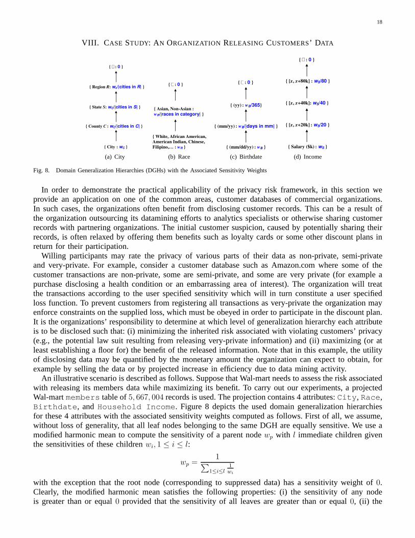
Fig. 8. Domain Generalization Hierarchies (DGHs) with the Associated Sensitivity Weights

In order to demonstrate the practical applicability of the privacy risk framework, in this section weprovide an application on one of the common areas, customer databases of commercial organizations.In such cases, the organizations often benefit from disclosing customer records. This can be a result ofthe organization outsourcing its datamining efforts to analytics specialists or otherwise sharing customerrecords with partnering organizations. The initial customer suspicion, caused by potentially sharing theirrecords, is often relaxed by offering them benefits such as loyalty cards or some other discount plans inreturn for their participation.

Willing participants may rate the privacy of various parts of their data as non-private, semi-privateand very-private. For example, consider a customer database such as Amazon.com where some of thecustomer transactions are non-private, some are semi-private, and some are very private (for example apurchase disclosing a health condition or an embarrassing area of interest). The organization will treatthe transactions according to the user specified sensitivity which will in turn constitute a user specifiedloss function. To prevent customers from registering all transactions as very-private the organization mayenforce constraints on the supplied loss, which must be obeyed in order to participate in the discount plan.It is the organizations’ responsibility to determine at which level of generalization hierarchy each attributeis to be disclosed such that: (i) minimizing the inherited risk associated with violating customers’ privacy(e.g., the potential law suit resulting from releasing very-private information) and (ii) maximizing (or atleast establishing a floor for) the benefit of the released information. Note that in this example, the utilityof disclosing data may be quantified by the monetary amount the organization can expect to obtain, forexample by selling the data or by projected increase in efficiency due to data mining activity.

An illustrative scenario is described as follows. Suppose that Wal-mart needs to assess the risk associatedwith releasing its members data while maximizing its benefit. To carry out our experiments, a projectedWal-martmembers table of5, 667, 004 records is used. The projection contains 4 attributes:City, Race,Birthdate, andHousehold Income. Figure 8 depicts the used domain generalization hierarchiesfor these 4 attributes with the associated sensitivity weights computed as follows. First of all, we assume,without loss of generality, that all leaf nodes belonging tothe same DGH are equally sensitive. We use amodified harmonic mean to compute the sensitivity of a parentnodewp with l immediate children giventhe sensitivities of these childrenwi, 1 ≤ i ≤ l:

wp =1∑

1≤i≤l1wi

with the exception that the root node (corresponding to suppressed data) has a sensitivity weight of0.Clearly, the modified harmonic mean satisfies the following properties: (i) the sensitivity of any nodeis greater than or equal0 provided that the sensitivity of all leaves are greater thanor equal0, (ii) the

19

sensitivity of a parent node is always less than or equal (in case of1 child) the sensitivity of any of itsdescendent nodes, and (iii) the higher the number of children a node has the lower the sensitivity of thisnode.

For example, given a constant city weightwc, the weight of theCounty nodej in the DGH for theCity is 1∑

1≤i≤lj

1

wc

= wc

lj, wherelj is the number of cities in the countyj. Moreover, the sensitivity of

theState node in the same DGH is 1∑1≤j≤m

1

wc/lj

= wc∑1≤j≤m lj

= wc

n, wherem is the number of counties

in the state andn =∑

1≤j≤m lj is the number of cities in the state.The multiplicative formΦ4(y) of the sensitivity function is used to compute the overall sensitivity of a

released record. The weightswc, wr, wb, andws are set at the values0.3, 0.4, 0.5, and0.75, respectively.Therefore, the sensitivity associated with the record(West Lafayette, White, 05/10/1975,$52k), for example, ise0.3+0.4+0.5+0.75 = 7.03, whereas the sensitivity associated with the record(WestLafayette, ⊥, May 1975, [$20k,$99k]) is e0.3+0+ 0.5

31+ 0.75

80 = 1.38.We use the Adult database1 which is comprised of9, 857, 623 records extracted from US Census data as a

dictionaryθ. The database contains 5 attributes:Age, Gender, Zipcode, Race, andEducation. Eachrecordy (and its generalizations) from Wal-martmembers table is matched with this dictionary to identifythe number of dictionary records consistent with itρ(δ(y)). The matching process is performed on thecorresponding attributes representing age, race, and address in both tables. For example, the record(WestLafayette, White, 05/10/1975, $52k) has7 dictionary records consistent with it, whereasthe record(West Lafayette, ⊥, May 1975, [$20k,$99k]) has198 dictionary records con-sistent with it.

The loss function associated with releasing a recordy is ℓ(y, θ) = Φ(y)|ρ(y,θ)|

. For example, from the aboveresults, the loss associated with releasing the record(West Lafayette, White, 05/10/1975,$52k) is 7.03/7 = 1.004, whereas the loss associated with releasing the record(West Lafayette,⊥, May 1975, [$20k,$99k]) is 1.38/198 = 0.007. The overall risk associated with releasing awhole table is computed as the average loss associated with releasing its individual records.

We use the same utility function explained in Section VII-B.For example, the utility function corre-sponding to the record(West Lafayette, White, 05/10/1975, $52k) is 4 + 2 + 3 + 4 =13 or equivalently(4 + 2 + 3 + 4) − (0) = 13, whereas the utility function corresponding to therecord(West Lafayette, ⊥, May 1975, [$20k,$99k]) is 4 + 0+ 2 + 1 = 7 or equivalently(4 + 2 + 3 + 4) − (0 + 2 + 1 + 3) = 7.

By following the procedure explained above, the organization goal to determine the disclosure rule thatyields the minimal risk while maintaining the utility abovea certain threshold is achievable. For eachpotentially disclosed tableT , our model can be applied to assess both the risk and utility associated withreleasing this table. As the case with the risk, the utility of a given table is the average utility of allindividual records constituting this table rounded to the nearest integer. The table that poses the minimalrisk with an acceptable utility is released.

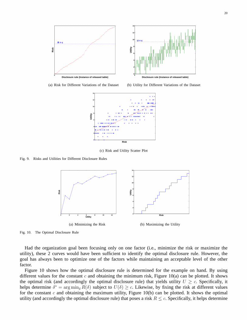
Figure 9 shows some plots of the risks and associated utilities for various disclosure rules. Recall that adisclosure ruleδi(T ) (or simply δi) is a combination of transformations (suppression, generalization, anddisclosure of actual data) performed on the attributes of the original tableT which results in the tableT ′ tobe released2. Figures 9(a)(b) plot the computed risks (in increasing order) and the corresponding utilitiesfor random instances of the released tableT ′, R = {

(δi, R(δi, θ)

), i = 1, 2, · · · } andU = {

(δi, U(δi)

), i =

1, 2, · · · }, respectively. As pointed out earlier, the trend is that theutility increases as the risk increases.However, sometimes this is not the case due to the settings ofthe sensitivity weights and the topologiesof different DGHs. The scatter plot in Figure 9(c) depicts the high positive correlations between risk andutility with a computed correlation coefficient of0.858.

1Downloaded fromhttp://www.ipums.org.2An example of T ′ is {(West Lafayette,White,05/10/1975,$52k), (Indiana,Asian,1948,⊥),

(⊥,Chinese,August 1965,[$20k,$40k]), · · · }.

20

0Disclosure rule (Instance of released table)

Ris

k

R = c

(a) Risk for Different Variations of the Dataset

00

2

4

6

8

10

12

14

Disclosure rule (Instance of released table)

Uti

lity

U = c

(b) Utility for Different Variations of the Dataset

0

2

4

6

8

10

12

14

Risk

Uti

lity

(c) Risk and Utility Scatter Plot

Fig. 9. Risks and Utilities for Different Disclosure Rules

0 2 4 6 8 10 12Utility

Ris

k

(a) Minimizing the Risk

0

2

4

6

8

10

12

14

Risk

Uti

lity

(b) Maximizing the Utility

Fig. 10. The Optimal Disclosure Rule

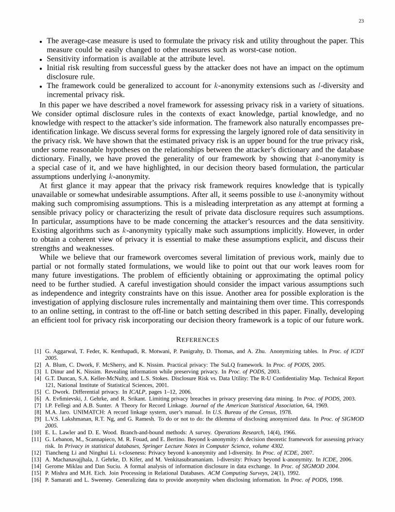
Had the organization goal been focusing only on one factor (i.e., minimize the risk or maximize theutility), these 2 curves would have been sufficient to identify the optimal disclosure rule. However, thegoal has always been to optimize one of the factors while maintaining an acceptable level of the otherfactor.

Figure 10 shows how the optimal disclosure rule is determined for the example on hand. By usingdifferent values for the constantc and obtaining the minimum risk, Figure 10(a) can be plotted.It showsthe optimal risk (and accordingly the optimal disclosure rule) that yields utilityU ≥ c. Specifically, ithelps determineδ∗ = arg minδ R(δ) subject toU(δ) ≥ c. Likewise, by fixing the risk at different valuesfor the constantc and obtaining the maximum utility, Figure 10(b) can be plotted. It shows the optimalutility (and accordingly the optimal disclosure rule) thatposes a riskR ≤ c. Specifically, it helps determine

21

1 2 3 4 50

500

1000

1500

Utility threshold

Occ

ure

nce

s (1

k)

actual citycountystateregionhidden

(a) City

1 2 3 4 50

500

1000

1500

Utility threshold

Occ

ure

nce

s (1

k)

actual raceAsian/Non−Asianhidden

(b) Race

1 2 3 4 50

500

1000

1500

Utility threshold

Occ

ure

nce

s (1

k)

actual BDmm/yyyyhidden

(c) Birthdate

1 2 3 4 50

500

1000

1500

Utility threshold

Occ

ure

nce

s (1

k)

actual salary ($k)$20k range$40k range$80k rangehidden

(d) Salary

Fig. 11. Effect of Utility Threshold on the Level of Attribute Disclosure

δ∗ = arg maxδ U(δ) subject toR(δ) ≤ c.We implemented a heuristic discrete optimization algorithm, Branch and Bound [10], to obtain the

heuristic optimum disclosure rule. Figure 12 shows that thediscrete optimization algorithm is superior interms of execution time compared to the brute-force algorithm with no significant risk increase.

Figure 11 shows some statistics about the frequencies of generalization steps carried out on eachattribute at different utility levels to obtain the optimalrisk. For instance, when setting the utilityU ≥ 5,Figure 11(d) indicates that the actual salaries of almost all members are released. Clearly, the tendencytowards releasing the actual data increases as the utility level increases. Moreover, depending on attributesettings, the level of aggressiveness with which the tendency to release the actual data occurs varies. Thestatistics shows, for instance, that most of the time the actual birthdate is released when the requiredutility U ≥ 3. An organization that is willing to apply the disclosure rule which has been applied themost may elect to release the actual birthdate for a newly added record when the utility is sought to beno less than3.

IX. RELATED WORK

In [11] we consider the optimal disclosure rule, based solely on data suppression, that yields theminimum risk subject to a maximum number of suppressed data items. Incorporating data generalizationinto the privacy risk framework is a new contribution of thispaper and was not part of the work presentedin [11]. Furthermore, utility functions were not addressedin the optimization model presented in [11].The optimization model presented in this paper takes into account both risk minimization and utilitymaximization. A new set of experiments are conducted in thispaper that shows the superiority of privacyrisk obtained by applying our framework as opposed to that obtained fromk-anonymity for the sameutility level. A complete and detailed test case is providedin this paper, and was not present in [11], thatwalks the reader through various stages of our framework in detail and clarifies different computations.

22

0 2 4 6 8 10 12Utility

Ris

k

optimal algorithmdiscrete optimation

(a) Risk

0 1 2 3 4 5 6

x 104

0

0.5

1

1.5

2

2.5

3

3.5

4

4.5x 10

4

Table size (records)

Tim

e (s

ec)

optimal algorithmdiscrete optimization

(b) Time

Fig. 12. The Discrete Optimization Algorithm

Section V relates the privacy risk framework tok-anonymity. In this section, we discuss additionalrelated work from statistical databases and data mining. Instatistical databases, queries result in somestatistical information, for example the average of a set ofvalues. The techniques for preserving privacycan be divided into two categories: (i) query restriction and (ii) input-output perturbation. Query restrictionmethods pose limitations on query parameters while input-output perturbations alter the data by introducingnoise to either the data or the query results. Unlike statistical databases that are concerned with disclosingstatistical data summaries, our framework focuses on disclosing elementary data and thus incorporatesa broader class of queries. Moreover, while recent proposals in statistical database [3], [2] focus on thetradeoff between meaningfulness of information and privacy loss, we are interested in the fundamentallydifferent tradeoff between disclosure benefit and privacy loss. In the data mining area, several approacheshave been developed for privacy preserving data mining. Unlike our approach, such approaches (e.g., [6])are based on perturbing the original data and at the same timeachieving correct data mining results.

Duncan et al. [4] describes a framework, called Risk-Utility (R-U) confidentiality map, which addressesthe tradeoff between data utility and disclosure. Lakshmanan et al. [9] propose an approach to the riskanalysis for disclosed anonymized data; such approach models a database as series of transactions andthe attacker’s knowledge as a belief function. Our model is fundamentally different since we deal exactlywith relational instances rather than data frequencies, wedo not consider simply anonymized data and weincorporate the concept of data sensitivity into our framework. Miklau and Suciu [14] provide a measureof the privacy risk in the context of the query-view securityproblem, but such measure does not resultin a complete framework for privacy risk assessment.

In summary, the goal of avoiding privacy breaches has been investigated by different communities.Nevertheless, to the best of our knowledge, our approach is the first in providing a comprehensivetheoretical framework for assessing privacy risks. Our framework is based on statistical decision theoryand is a highly flexible tool for modeling the trade-off between disclosure benefits and risks. Moreover,it incorporates the notion of data sensitivity. Besides resulting in a clear probabilistic interpretation, theconnection to decision theory may be exploited in deriving additional results based on the vast literaturein that topic.

X. D ISCUSSION

Privacy Risk Framework Assumptions:• Protection is provided in terms of masking values (data suppression and/or generalization) regardless

of the information that the attacker may imply by masking outthese values.• It is assumed that the adversarial external knowledge is in terms of a side information referred to as

a dictionary.

23

• The average-case measure is used to formulate the privacy risk and utility throughout the paper. Thismeasure could be easily changed to other measures such as worst-case notion.

• Sensitivity information is available at the attribute level.• Initial risk resulting from successful guess by the attacker does not have an impact on the optimum

disclosure rule.• The framework could be generalized to account fork-anonymity extensions such asl-diversity and

incremental privacy risk.In this paper we have described a novel framework for assessing privacy risk in a variety of situations.

We consider optimal disclosure rules in the contexts of exact knowledge, partial knowledge, and noknowledge with respect to the attacker’s side information.The framework also naturally encompasses pre-identification linkage. We discuss several forms for expressing the largely ignored role of data sensitivity inthe privacy risk. We have shown that the estimated privacy risk is an upper bound for the true privacy risk,under some reasonable hypotheses on the relationships between the attacker’s dictionary and the databasedictionary. Finally, we have proved the generality of our framework by showing thatk-anonymity isa special case of it, and we have highlighted, in our decisiontheory based formulation, the particularassumptions underlyingk-anonymity.

At first glance it may appear that the privacy risk framework requires knowledge that is typicallyunavailable or somewhat undesirable assumptions. After all, it seems possible to usek-anonymity withoutmaking such compromising assumptions. This is a misleadinginterpretation as any attempt at forming asensible privacy policy or characterizing the result of private data disclosure requires such assumptions.In particular, assumptions have to be made concerning the attacker’s resources and the data sensitivity.Existing algorithms such ask-anonymity typically make such assumptions implicitly. However, in orderto obtain a coherent view of privacy it is essential to make these assumptions explicit, and discuss theirstrengths and weaknesses.

While we believe that our framework overcomes several limitation of previous work, mainly due topartial or not formally stated formulations, we would like to point out that our work leaves room formany future investigations. The problem of efficiently obtaining or approximating the optimal policyneed to be further studied. A careful investigation should consider the impact various assumptions suchas independence and integrity constraints have on this issue. Another area for possible exploration is theinvestigation of applying disclosure rules incrementallyand maintaining them over time. This correspondsto an online setting, in contrast to the off-line or batch setting described in this paper. Finally, developingan efficient tool for privacy risk incorporating our decision theory framework is a topic of our future work.

REFERENCES

[1] G. Aggarwal, T. Feder, K. Kenthapadi, R. Motwani, P. Panigrahy, D. Thomas, and A. Zhu. Anonymizing tables. InProc. of ICDT2005.

[2] A. Blum, C. Dwork, F. McSherry, and K. Nissim. Practical privacy: The SuLQ framework. InProc. of PODS, 2005.[3] I. Dinur and K. Nissim. Revealing information while preserving privacy. InProc. of PODS, 2003.[4] G.T. Duncan, S.A. Keller-McNulty, and L.S. Stokes. Disclosure Risk vs. Data Utility: The R-U Confidentiality Map. Technical Report

121, National Institute of Statistical Sciences, 2001.[5] C. Dwork. Differential privacy. InICALP, pages 1–12, 2006.[6] A. Evfimievski, J. Gehrke, and R. Srikant. Limiting privacy breaches in privacy preserving data mining. InProc. of PODS, 2003.[7] I.P. Fellegi and A.B. Sunter. A Theory for Record Linkage. Journal of the American Statistical Association, 64, 1969.[8] M.A. Jaro. UNIMATCH: A record linkage system, user’s manual. In U.S. Bureau of the Census, 1978.[9] L.V.S. Lakshmanan, R.T. Ng, and G. Ramesh. To do or not to do: the dilemma of disclosing anonymized data. InProc. of SIGMOD

2005.[10] E. L. Lawler and D. E. Wood. Branch-and-bound methods: Asurvey. Operations Research, 14(4), 1966.[11] G. Lebanon, M., Scannapieco, M. R. Fouad, and E. Bertino. Beyond k-anonymity: A decision theoretic framework for assessing privacy

risk. In Privacy in statistical databases, Springer Lecture Notes in Computer Science, volume 4302.[12] Tiancheng Li and Ninghui Li. t-closeness: Privacy beyond k-anonymity and l-diversity. InProc. of ICDE, 2007.[13] A. Machanavajjhala, J. Gehrke, D. Kifer, and M. Venkitasubramaniam. l-diversity: Privacy beyond k-anonymity. InICDE, 2006.[14] Gerome Miklau and Dan Suciu. A formal analysis of information disclosure in data exchange. InProc. of SIGMOD 2004.[15] P. Mishra and M.H. Eich. Join Processing in Relational Databases.ACM Computing Surveys, 24(1), 1992.[16] P. Samarati and L. Sweeney. Generalizing data to provide anonymity when disclosing information. InProc. of PODS, 1998.

24

[17] P. Samarati and L. Sweeney. Protecting privacy when disclosing information: k-anonymity and its enforcement through generalizationand suppression. Technical report, SRI International, 1998.

[18] R. P. Stanley.Enumerative Combinatorics, volume 1. Wadsworth & Brooks/Cole Mathematics Series, 1986.[19] L. Sweeney. Privacy-enhanced linking.ACM SIGKDD Explorations, 7(2), 2005.[20] U.S. Federal Geographic Data Committee. Guidelines for providing appropriate access to geospatial data in response to security

concerns, 2005.http://fgdc.er.usgs.gov/fgdc/homeland/access guidelines.pdf.[21] A. Wald. Statistical Decision Functions. Wiley, 1950.[22] Joe Whittaker.Graphical models in applied multivariate analysis. John Wiley and sons, 1990.[23] W.E. Winkler. Methods for Evaluating and Creating DataQuality. Information Systems, 29(7), 2004.[24] X. Xiao and Y. Tao. Personalized privacy preservation.In Proc. of SIGMOD, 2006.[25] S. Zhong, Z. Yang, and R.N. Wright. Privacy-enhancing k-anonymization of customer data. InProc. of PODS 2005.