Certifiable Robustness and Robust Training forGraph Convolutional Networks

Daniel Zügner Stephan Günnemann

Technical University of Munich, Germany

zuegnerd,guennemann@in.tum.de

ABSTRACT

Recent works show that Graph Neural Networks (GNNs) are highly

non-robust with respect to adversarial attacks on both the graph

structure and the node attributes, making their outcomes unreliable.

We propose the first method for certifiable (non-)robustness of

graph convolutional networks with respect to perturbations of the

node attributes1. We consider the case of binary node attributes

(e.g. bag-of-words) and perturbations that are L0-bounded. If a nodehas been certified with our method, it is guaranteed to be robust

under any possible perturbation given the attack model. Likewise,

we can certify non-robustness. Finally, we propose a robust semi-

supervised training procedure that treats the labeled and unlabeled

nodes jointly. As shown in our experimental evaluation, our method

significantly improves the robustness of the GNNwith onlyminimal

effect on the predictive accuracy.

ACM Reference Format:

Daniel Zügner and Stephan Günnemann. 2019. Certifiable Robustness and

Robust Training for Graph Convolutional Networks. In The 25th ACMSIGKDD Conference on Knowledge Discovery and Data Mining (KDD ’19),August 4–8, 2019, Anchorage, AK, USA. ACM, New York, NY, USA, 11 pages.

https://doi.org/10.1145/3292500.3330905

1 INTRODUCTION

Graph data is the core for many high impact applications rang-

ing from the analysis of social networks, over gene interaction

networks, to interlinked document collections. One of the most

frequently applied tasks on graph data is node classification: givena single large (attributed) graph and the class labels of a few nodes,

the goal is to predict the labels of the remaining nodes. Applica-

tions include the classification of proteins in interaction graphs

[9], prediction of customer types in e-commerce networks [6], or

the assignment of scientific papers from a citation network into

topics [12]. While there exist many classical approaches to node

classification [2, 15], recently graph neural networks (GNNs), alsocalled graph convolutional networks, have gained much attention

and improved the state of the art in node classification [5, 7, 12, 13].

However, there is one big catch: Recently it has been shown that

such approaches are vulnerable to adversarial attacks [4, 21, 22]:

1Code available at https://www.kdd.in.tum.de/robust-gcn

Permission to make digital or hard copies of all or part of this work for personal or

classroom use is granted without fee provided that copies are not made or distributed

for profit or commercial advantage and that copies bear this notice and the full citation

on the first page. Copyrights for components of this work owned by others than the

author(s) must be honored. Abstracting with credit is permitted. To copy otherwise, or

republish, to post on servers or to redistribute to lists, requires prior specific permission

and/or a fee. Request permissions from permissions@acm.org.

KDD ’19, August 4–8, 2019, Anchorage, AK, USA© 2019 Copyright held by the owner/author(s). Publication rights licensed to ACM.

ACM ISBN 978-1-4503-6201-6/19/08. . . $15.00

https://doi.org/10.1145/3292500.3330905

Even only slight deliberate perturbations of the nodes’ features

or the graph structure can lead to completely wrong predictions.

Such negative results significantly hinder the applicability of these

models. The results become unreliable and such problems open the

door for attackers that can exploit these vulnerabilities.

So far, no effective mechanisms are available, which (i) prevent

that small changes to the data lead to completely different predic-

tions in a GNN, or (ii) that can verify whether a given GNN is robust

w.r.t. specific perturbation model. This is critical, since especially

in domains where graph-based learning is used (e.g. the Web) ad-

versaries are omnipresent, e.g., manipulating online reviews and

product websites [11]. One of the core challenges is that in a GNN

a node’s prediction is also affected when perturbing other nodes inthe graph – making the space of possible perturbations large. How

to make sure that small changes to the input data do not have a

dramatic effect to a GNN?

In this work, we shed light on this problem by proposing the

first method for provable robustness of GNNs. More precisely, we

focus on graph convolutional networks and potential perturbations

of the node attributes, where we provide:

1) Certificates: Given a trained GNN, we can give robustness cer-

tificates that state that a node is robust w.r.t. a certain space of

perturbations. If the certificate holds, it is guaranteed that no per-turbation (in the considered space) exists which will change the

node’s prediction. Furthermore, we also provide non-robustness

certificates that, when they hold, state whether a node is not

robust; realized by providing an adversarial example.

2) Robust Training: We propose a learning principle that improves

the robustness of the GNN (i.e. making it less sensitive to pertur-

bations) while still ensuring high accuracy for node classification.

Specifically, we exploit the semi-supervised nature of the GNN

learning task, thus, taking also the unlabeled nodes into account.

In contrast to existing works on provable robustness for classical

neural networks/robust training (e.g. [10, 18, 20]), we tackle various

additional challenges: Being the first work for graphs, we have to

deal with perturbations of multiple instances simultaneously. For

this, we introduce a novel space of perturbations where the pertur-

bation budget is constrained locally and globally. Moreover, since

the considered data domains are often discrete/binary attributes,

we tackle challenging L0 constraints on the perturbations. Lastly,

we exploit a crucial aspect of semi-supervised learning by taking

also the unlabeled nodes into account for robust training.

The key idea we will exploit in our work is to estimate the worst-case change in the predictions obtained by the GNN under the

space of perturbations. If the worst possible change is small, the

GNN is robust. Since, however, this worst-case cannot be computed

efficiently, we provide bounds on this value, providing conservative

arX

iv:1

906.

1226

9v1

[cs

.LG

] 2

8 Ju

n 20

19

estimates. More technically, we derive relaxations of the GNN and

the perturbations space, enabling efficient computation.

Besides the two core technical contributions mentioned above,

we further perform extensive experiments:

3) Experiments: We show on various graph datasets that GNNs

trained in the traditional way are not robust, i.e. only few of

the nodes can be certified to be robust, respectively many are

certifiably non-robust even with small perturbation budgets. In

contrast, using our robust training we can dramatically improve

robustness increasing it by in some cases by factor of four.

Overall, using our method, significantly improves the reliability of

GNNs, thus, being highly beneficial when, e.g., using them in real

production systems or scientific applications.

2 RELATEDWORK

The sensitivity of machine learning models w.r.t. adversarial pertur-

bations has been studied extensively [8] . Only recently, however,

researchers have started to investigate adversarial attacks on graph

neural networks [4, 21, 22] and node embeddings [1]. All of these

works focus on generating adversarial examples. In contrast, we

provide the first work to certify and improve the robustness of

GNNs. As shown in [21], both perturbations to the node attributes

as well as the graph structure are harmful. In this work, we fo-

cus on perturbations of the node attributes and we leave structure

perturbations for future work.

For ‘classical’ neural networks various heuristic approaches have

been proposed to improve the the robustness to adversarial exam-

ples [17]. However, such heuristics are often broken by new attack

methods, leading to an arms race. As an alternative, recent works

have considered certifiable robustness [3, 10, 18, 20] providing guar-

antees that no perturbation w.r.t. a specific perturbation space will

change an instance’s prediction.

For this work, specifically the class of methods based on convex

relaxations are of relevance [18, 20]. They construct a convex re-

laxation for computing a lower bound on the worst-case margin

achievable over all possible perturbations. This bound serves as a

certificate of robustness. Solving such convex optimization prob-

lems can often been done efficiently, and by exploiting duality it

enables to even train a robust model [20]. As already mentioned,

our work differs significantly from the existing methods since (i)

it considers the novel GNN domain with its relational dependen-

cies, (ii) it handles a discrete/binary data domain, while existing

works have only handled continuous data; thus also leading to

very different constraints on the perturbations, and (iii) we propose

a novel robust training procedure which specifically exploits the

semi-supervised learning setting of GNNs, i.e. using the unlabeled

nodes as well.

3 PRELIMINARIES

We consider the task of (semi-supervised) node classification in

a single large graph having binary node features. Let G = (A,X )be an attributed graph, where A ∈ 0, 1N×N

is the adjacency

matrix and X ∈ 0, 1N×Drepresents the nodes’ features. W.l.o.g.

we assume the node-ids to be V = 1, . . . ,N . Given a subset

VL ⊆ V of labeled nodes, with class labels from C = 1, 2, . . . ,K,the goal of node classification is to learn a function f : V → C

which maps each node v ∈ V to one class in C. In this work, we

focus on node classification employing graph neural networks. In

particular, we consider graph convolutional networks where the

latent representations H (l )at layer l are of the form

H (l ) = σ (l )(A(l−1)

H (l−1)W (l−1) + b(l−1))for l = 2, ...,L (1)

where H (1) = X and with activation functions given by

σ (L) (·) = softmax (·) , σ (l ) (·) = ReLU (·) for l = 2, ...,L − 1.

The output H (L)vc denotes the probability of assigning node v to

class c . The A(l )

are the message passing matrices that define how

the activations are propagated in the network. In GCN [12], for

example, A(1)= ... = A

(L−1)= ˜D− 1

2 A ˜D− 1

2 , where A = A + IN×Nand

˜Dii =∑j Ai j . TheW (.)

and b(.) are the trainable weights ofthe graph neural network, usually simply learned by minimizing

the cross-entropy loss on the given labeled training nodesVL .

Notations: We denote with Nl (t) the l-hop neighborhood of a

node t , i.e. all nodes which are reachable with l hops (or less) fromnode t , including the node t itself. Given a matrix X , we denote its

positive part with [X ]+ = max(X , 0)where themax is applied entry-

wise. Similarly, the negative part is [X ]− = −min(X , 0), whichare non-negative numbers. All matrix norms | |X | |p used in the

paper are meant to be entry-wise, i.e. flattening X to a vector and

applying the corresponding vector norm. We denote with h(l ) the

dimensionality of the latent space in layer l , i.e.H (l ) ∈ RN×h(l ). Xi :

denotes the i-th row of a matrix X and X:j its j-th column.

4 CERTIFYING ROBUSTNESS FOR GRAPH

CONVOLUTIONAL NETWORKS

Our first goal is to derive an efficient principle for robustness cer-

tificates. That is, given an already trained GNN and a specific node

t under consideration (called target node), our goal is to provide a

certificate which guarantees that the prediction made for node t willnot change even if the data gets perturbed (given a specific pertur-

bation budget). That is, if the certificate is provided, the prediction

for this node is robust under any admissible perturbations. Unlike

existing works, we cannot restrict perturbations to the instance

itself due to the relational dependencies.

However, we can exploit one key insight: for a GNN with L

layers, the output H (L)t : of node t depends only on the nodes in its

L − 1 hop neighborhood NL−1(t). Therefore, instead of operating

with Eq. (1), we can ‘slice’ the matrices X and A(l )

at each step to

only contain the entries that are required to compute the output

for the target node t .2 This step drastically improves scalability

– reducing not only the size of the neural network but also the

potential perturbations we have to consider later on. We define the

matrix slices for a given target t as follows:3

ÛA(l )= A

(l )NL−l (t ),NL−l+1(t ) for l = 1, ...,L − 1, ÛX = XNL−1(t ): (2)

where the set indexing corresponds to slicing the rows and columns

of a matrix, i.e. AN2(t ),N1(t ) contains the rows corresponding to the

2Note that the shapes ofW and b do not change.

3To avoid clutter in the notation, since our method certifies robustness with respect to

a specific node t , we omit explicitly mentioning the target node t in the following.

two-hop neighbors of node t and the columns corresponding to its

one-hop neighbors. As it becomes clear, for increasing l (i.e. depth

in the network), the slices of A(l )

become smaller, and at the final

step we only need the target node’s one-hop neighbors.

Overall, we only need to consider the following sliced GNN:

H(l )= ÛA(l−1)

H (l−1)W (l−1) + b(l−1) for l = 2, ...,L (3)

H (l )nj = max

H

(l )nj , 0

for l = 2, ...,L − 1 (4)

and H (1) = ÛX . Here, we replaced the ReLU activation by its ana-

lytical form, and we denoted with H(l )

the input before applying

the ReLU, and with H (l )the corresponding output. Note that the

matrices are getting smaller in size – with H(L)

actually reducing

to a vector that represents the predicted log probabilities (logits)

for node t only. Note that we also omitted the softmax activation

function in the final layer L since for the final classification decision

it is sufficient to consider the largest value of H(L)

. Overall, we

denote the output of this sliced GNN as f tθ ( ÛX , ÛA) = H(L) ∈ RK .

Here θ is the set of all parameters, i.e. θ = W (·),b(·).

4.1 Robustness Certificates for GNNs

Given this set-up, we are now ready to define our actual task: We

aim to verify whether no admissible perturbation changes the pre-

diction of the target node t . Formally we aim to solve:

Problem 1. Given a graph G, a target node t , and an GNN withparameters θ . Let y∗ denote the class of node t (e.g. given by theground truth or predicted). The worst case margin between classes y∗

and y achievable under some setXq,Q ( ÛX ) of admissible perturbationsto the node attributes is given by

mt (y∗,y) := minimize

˜Xf tθ ( ˜X , ÛA)y∗ − f tθ ( ˜X , ÛA)y (5)

subject to˜X ∈ Xq,Q ( ÛX )

Ifmt (y∗,y) > 0 for all y , y∗, the GNN is certifiably robust w.r.t.node t and Xq,Q .

If the minimum in Eq. (5) is positive, it means that there exists noadversarial example (within our defined admissible perturbations)

that leads to the classifier changing its prediction to the other class

y – i.e. the logits of class y∗ are always larger than the one of y.Setting reasonable constraints to adversarial attacks is important

to obtain certificates that reflect realistic attacks. Works for classicalneural networks have constrained the adversarial examples to lie

on a small ϵ-ball around the original sample measured by, e.g., the

infinity-norm or L2-norm [3, 18, 20], often e.g. ϵ < 0.1 This is

clearly not practical in our binary setting as an ϵ < 1 would mean

that no attribute can be changed. To allow reasonable perturbations

in a binary/discrete setting one has to allow much larger changes

than the ϵ-balls considered so far.

Therefore, motivated by the existingworks on adversarial attacks

to graphs [21], we consider a more realistic scenario: We define the

set of admissible perturbations by limiting the number of changes tothe original attributes – i.e. we assume a perturbation budgetQ ∈ Nand measure the L0 norm in the change to

ÛX . It is important to note

that in a graph setting an adversary can attack the target node by

also changing the node attributes of its L − 1 hop neighborhood.

Thus, Q acts as a global perturbation budget.

However, since changing many attributes for a single node might

not be desired, we also allow to limit the number of perturbations

locally – i.e. for each node in the L − 1 hop neighborhood we can

consider a budget of q ∈ N. Overall, in this work we consider

admissible perturbations of the form:

Xq,Q ( ÛX ) =˜X ˜Xnj ∈ 0, 1 ∧ ∥ ˜X − ÛX ∥0 ≤ Q (6)

∧ ∥ ˜Xn: − ÛXn:∥0 ≤ q ∀n ∈ NL−1.

Challenges: There are two major obstacles preventing us from

efficiently finding the minimum in Eq. (5). First, our data domain is

discrete, making optimization often intractable. Second, our func-

tion (i.e. the GNN) f tθ is nonconvex due to the nonlinear activation

functions in the neural network. But there is hope: As we will show,

we can efficiently find lower bounds on the minimum of the orig-

inal problem by performing specific relaxations of (i) the neural

network, and (ii) the data domain. This means that if the lower

bound is positive, we are certain that our classifier is robust w.r.t.

the set of admissible perturbations. Remarkably, we will even see

that our relaxation has an optimal solution which is integral. That

is, we obtain an optimal solution (i.e. perturbation) which is binary

– thus, we can effectively handle the discrete data domain.

4.2 Convex Relaxations

To make the objective function in Eq. (5) convex, we have to find

a convex relaxation of the ReLU activation function. While there

are many ways to achieve this, we follow the approach of [20] in

this work. The core idea is (i) to treat the matrices H (·)and H

(·)

in Eqs. (3,4) no longer as deterministic but as variables one can

optimize over (besides optimizing over˜X ). In this view, Eqs. (3,4)

become constraints the variables have to fulfill. Then, (ii) we relax

the non-linear ReLU constraint of Eq. (4) by a set of convex ones.

In detail: Consider Eq. (4). Here, H(l )nj denotes the input to the

ReLU activation function. Let us assume we have given some lower

bounds R(l )nj and upper bounds S(l )nj on this input based on the pos-

sible perturbations (in Section 4.5 we will discuss how to find these

bounds). We denote with I(l )the set of all tuples (n, j) in layer

l for which the lower and upper bounds differ in their sign, i.e.

R(l )nj < 0 < S(l )nj . We denote with I(l )+ and I(l )

− the tuples where both

bounds are non-negative and non-positive, respectively.

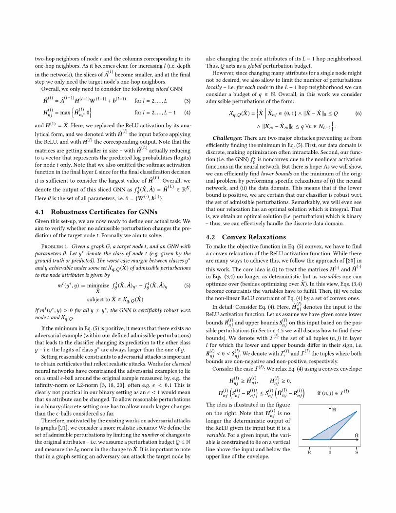
Consider the case I(l ): We relax Eq. (4) using a convex envelope:

H (l )nj ≥ H

(l )nj , H (l )

nj ≥ 0,

H (l )nj

(S(l )nj − R(l )nj

)≤ S(l )nj

(H

(l )nj − R(l )nj

)if (n, j) ∈ I(l )

R 0 S

H

H

The idea is illustrated in the figure

on the right. Note that H (l )nj is no

longer the deterministic output of

the ReLU given its input but it is a

variable. For a given input, the vari-

able is constrained to lie on a vertical

line above the input and below the

upper line of the envelope.

Accordingly, but more simply, for the cases I(l )+ and I(l )

− we get:

H (l )nj = H

(l )nj if (n, j) ∈ I(l )

+ H (l )nj = 0 if (n, j) ∈ I(l )

−

which are actually not relaxations but exact conditions. Overall,

Eq. (4) has now been replaced by a set of linear (i.e. convex) con-

straints. Together with the linear constraints of Eq. (3) they deter-

mine the set of admissible H (·)and H

(·)we can optimize over. We

denote the collection of these matrices that fulfill these constraints

by Zq,Q ( ˜X ). Note that this set depends on ˜X since H (1) = ˜X .

Overall, our problem becomes:

mt (y∗,y) := minimize

˜X ,H (·),H(·)

H(L)y∗ − H

(L)y = c⊤H

(L)(7)

subject to˜X ∈ Xq,Q ( ÛX ) , [H (·), H

(·)] ∈ Zq,Q ( ˜X )

Here we introduced the constant vector c = ey∗ − ey , which is 1

at position y∗, −1 at y, and 0 else. This notation clearly shows that

the objective function is a simple linear function.

Corollary 4.1. The minimum in Eq. (7) is a lower bound on theminimum of the problem in Eq. (5), i.e. mt (y∗,y) ≤ mt (y∗,y).

Proof. Let˜X be the perturbation obtained by Problem 1, and

[H (·), H(·)] the resulting exact representations based on Eq. (3)+(4).

By construction, [H (·), H(·)] ∈ Zq,Q ( ÛX ). Since Eq. (7) optimizes

over the full setZq,Q ( ÛX ) its minimum can not be larger.

From Corollary 4.1 it follows that if mt (y∗,y) > 0 for all y , y∗,the GNN is robust at node t . Directly solving Eq. (7), however, is

still intractable due to the discrete data domain.

As one core contribution, we will show that we can find the

optimal solution in a tractable way. We proceed in two steps: (i) We

first find a suitable continuous, convex relaxation of the discrete

domain of possible adversarial examples. (ii) We show that the

relaxed problem has an optimal solution which is integral; thus, by

our specific construction the solution is binary.

More precisely, we relax the set Xq,Q ( ÛX ) to:

ˆXq,Q ( ÛX ) =˜X ˜Xnj ∈ [0, 1] ∧ ∥ ˜X − ÛX ∥1 ≤ Q (8)

∧ ∥ ˜Xn: − ÛXn:∥1 ≤ q ∀n ∈ NL−1

Note that the entries of˜X are now continuous between 0 and 1,

and we have replaced the L0 norm with the L1 norm. This leads to:

mt (y∗,y) := minimize

˜X ,H (·),H(·)

H(L)y∗ − H

(L)y = c⊤H

(L)(9)

subject to˜X ∈ ˆXq,Q ( ÛX ) , [H (·), H

(·)] ∈ Zq,Q ( ˜X )

It is worth mentioning that Eq. (9) is a linear problem since besides

the linear objective function also all constraints are linear. We

provide the explicit form of this linear program in the appendix.

Accordingly, Eq. (9) can be solved optimally in a tractable way. Since

ˆXq,Q ( ÛX ) ⊃ Xq,Q ( ÛX ) , we trivially have mt (y∗,y) ≤ mt (y∗,y). Buteven more, we obtain:

Theorem 4.2. The minimum in Eq. (7) is equal to the minimumin Eq. (9), i.e. mt (y∗,y) = mt (y∗,y).

We will proof this theorem later (see Sec. 4.4) since it requires

some further results. In summary, using Theorem 4.2, we can indeed

handle the discrete data domain/discrete perturbations exactly and

tractably by simply solving Eq. (9) instead of Eq. (7).

4.3 Efficient Lower Bounds via the Dual

In order to provide a robustness guarantee w.r.t. the perturbationson

ÛX , we have to find the minimum of the linear program in Eq. (9)

to ensure that we have covered the worst case. While it is possible

to solve linear programs ‘efficiently’ using highly optimized linear

program solvers, the potentially large number of variables in a GNN

makes this approach rather slow. As an alternative, we can consider

the dual of the linear program [20]. There, any dual-feasible solutionis a lower bound on the minimum of the primal problem. That is, if

we find any dual-feasible solution for which the objective function

of the dual is positive, we know that the minimum of the primal

problem has to be positive as well, guaranteeing robustness of the

GNN w.r.t. any perturbation in the set.

Theorem 4.3. The dual of Eq. (9) is equivalent to:

maximize

Ω,η,ρдtq,Q

(ÛX ,c,Ω,η, ρ

)(10)

subject to

Ω(l ) ∈ [0, 1] |NL−l |×h(l )for l = L − 1, ..., 2,

η ∈ R |NL−1 |≥0 , ρ ∈ R≥0

where

дtq,Q (...) =L−1∑l=2

∑(n, j)∈I(l )

S(l )njR(l )nj

S(l )nj − R(l )nj

[ˆΦ(l )nj

]+−L−1∑l=1

1⊤Φ(l+1)b(l )

− Tr

[ÛX⊤

ˆΦ(1)]− ∥Ψ∥1 − q ·

∑n

ηn −Q · ρ

and

Φ(L) = −c ∈ Rk

ˆΦ(l ) = ÛA(l )⊤Φ(l+1)W (l )⊤ ∈ R |NL−l |×h(l )

for l = L − 1, ..., 1

Φ(l )nj =

0 if (n, j) ∈ I(l )

−ˆΦnj if (n, j) ∈ I(l )

+

S (l )nj

S (l )nj−R(l )nj

[ˆΦ(l )nj

]+− Ω(l )

nj

[ˆΦ(l )nj

]−

if (n, j) ∈ I(l )

for l = L − 1, ..., 2

Ψnd = max ∆nd − (ηn + ρ), 0

∆nd =[ˆΦ(1)nd

]+· (1 − ÛXnd ) +

[ˆΦ(1)nd

]−· ÛXnd

The proof is given in the appendix. Note that parts of the dual

problem in Theorem 4.3 have a similar form to the problem in [20].

For instance, we can interpret this dual problem as a backward pass

on a GNN, where theˆΦ(l )

and Φ(l )are the hidden representations

of the respective nodes in the graph. Crucially different, however,

is the propagation in the dual problem with the message passing

matricesÛA coming from the GNN formulation where neighboring

nodes influence each other. Furthermore, our novel perturbation

constraints from Eq. (8) lead to the dual variables η and ρ, which

have their origin in the local (q) and global (Q) constraints, respec-

tively. Note that, in principle, our framework allows for different

budgets q per node. The term Ψ has its origin in the constraint

˜Xnj ∈ [0, 1]. While on the first look, the above dual problem seems

rather complicated, its specific form makes it amenable for easyoptimization. The variables Ω,η, ρ have only simple, element-wise

constraints (e.g. clipping between [0, 1]). All other terms are just

deterministic assignments. Thus, straightforward optimization us-

ing (projected) gradient ascent in combination with any modern

automatic differentiation framework (e.g. TensorFlow, PyTorch) is

possible.

Furthermore, while in the above dual we need to optimize over

η and ρ, it turns out that we can simplify it even further: for any

feasible Ω, we get an optimal closed-form solution for η, ρ.

Theorem 4.4. Given the dual problem from Theorem 4.3 and anydual-feasible value for Ω. For each node n ∈ NL−1, let Sn be the setof dimensions d corresponding to the q largest values from the vector∆n: (ties broken arbitrarily). Further, denote with on = mind ∈Sn ∆ndthe smallest of these values. The optimal ρ that maximizes the dualis the Q-th largest value from [∆nd ]n∈NL−1,d ∈Sn . For later use wedenote with SQ the set of tuples (n,d) corresponding to theseQ-largestvalues. Moreover, the optimal ηn is ηn = max 0,on − ρ.

The proof is given in the appendix. Using Theo. 4.4, we obtain

an even more compact dual where we only have to optimize over

Ω. Importantly, the calculations done in Theo. 4.4 are also available

in many modern automatic differentiation frameworks (i.e. we can

back-propagate through them). Thus, we still get very efficient (and

easy to implement) optimization.

Default value: As mentioned before, it is not required to solve

the dual problem optimally. Any dual-feasible solution leads to a

lower bound on the original problem. Specifically, we can also just

evaluate the function дtq,Q once given a single instantiation for Ω.

This makes the computation of robustness certificates extremely

fast. For example, adopting the result of [20], instead of optimizing

over Ω we can set it to

Ω(l )nj = S(l )nj · (S

(l )nj − R(l )nj )

−1, (11)

which is dual-feasible, and still obtain strong robustness certificates.

In our experimental section, we compare the results obtained using

this default value to results for optimizing over Ω. Note that using

Theo. 4.4 we always ensure to use the optimal η, ρ w.r.t. Ω.

4.4 Primal Solutions and Certificates

Based on the above results, we can now prove the following:

Corollary 4.5. Eq. (9) is an integral linear program with respectto the variables ˜X .

The proof is given in the appendix. Using this result, it is now

straightforward to prove Theo. 4.2 from the beginning.

Proof. Since Eq. (9) has an optimal (thus, feasible) solution

where˜X is integral, we have

˜X ∈ ˆXq,Q ( ÛX ) and, thus, ˜X has to

be binary to be integral. Since in this case the L1 constraints are

equivalent to the L0 constraints, it follows that ˜X ∈ Xq,Q ( ÛX ). Thus,this optimal solution of Eq. 9 is feasible for Eq. 7 as well. Together

withmt (y∗,y) ≤ mt (y∗,y) it follows thatmt (y∗,y) = mt (y∗,y).

In the proof of Corollary 4.5, we have seen that in the optimal

solution, the set (n,d) ∈ SQ | ∆nd > 0 =: P indicates those

elements which are perturbed. That is, we constructed the worst-

case perturbation. Clearly, this mechanism can also be used even if

Ω (and, thus, ∆) is not optimal: simply perturbing the elements in

P . In this case, of course, the primal solution might not be optimal

and we cannot use it for a robustness certificate. However, since the

resulting perturbation is primal feasible (regarding the setXq,Q ( ÛX )),we can use it for our non-robustness certificate: After constructing

the perturbation˜X based on P , we pass it through the exact GNN,

i.e. we evaluate Eq. (5). If the value is negative, we found a harmful

perturbation, certifying non-robustness.

In summary: By considering the dual program, we obtain ro-

bustness certificates if the obtained (dual) values are positive for

everyy , y∗. In contrast, by constructing the primal feasible pertur-

bation using P , we obtain non-robustness certificates if the obtained(exact, primal) values are negative for one y , y∗. For some nodes,

neither of these certificates can be given. We analyze this aspect in

more detail in our experiments.

4.5 Activation Bounds

One crucial component of our method, the computation of the

bounds R(l ) and S(l ) on the activations in the relaxed GNN, remains

to be defined. Again, existing bounds for classical neural networks

are not applicable since they neither consider L0 constraints nor dothey take neighboring instances into account. Obtaining good upper

and lower bounds is crucial to obtain robustness certificates, as

tighter bounds lead to lower relaxation error of the GNN activations.

While in Sec. 4.3, we relax the discreteness condition of the node

attributesÛX in the linear program, it turns out that for the bounds

the binary nature of the data can be exploited. More precisely, for

every nodem ∈ NL−2(t), we compute the upper bound S(2)mj in the

second layer for latent dimension j as

S(2)mj = sum_top_Q

([ ÛA(1)

mnˆS(2)nji ]n∈N1(m),i ∈1, ...,q

)+ ÛH (2)

mj (12)

ˆS(2)nji = i-th_largest

((1 − ÛXn:) ⊙

[W (1)

:j

]++ ÛXn: ⊙

[W (1)

:j

]−

)Here, i-th_largest(·) denotes the selection of the i-th largest element

from the corresponding vector, and sum_top_Q(·) the sum of theQlargest elements from the corresponding list. The first term of the

sum in Eq. (12) is an upper bound on the change/increase in the first

hidden layer’s activations of nodem and hidden dimension j for any

admissible perturbation on the attributesÛX . The second term are

the hidden activations obtained for the (un-perturbed) inputÛX , i.e.

ÛH (2)mj =

ÛA(1) ÛXW (1) + b(1). In sum we have an upper bound on the

hidden activations in the first hidden layer for the perturbed input

˜X . Note that, reflecting the interdependence of nodes in the graph,

the bounds of a nodem depend on the attributes of its neighbors n.Likewise for the lower bound we use:

R(2)mj = - sum_top_Q

([ ÛA(1)

mnˆR(2)nji ]n∈N1(m),i ∈1, ...,q

)+ ÛH (2)

mj (13)

ˆR(2)nji = i-th_largest

(ÛXn: ⊙

[W (1)

:j

]++ (1 − ÛXn:) ⊙

[W (1)

:j

]−

)We need to compute the bounds for each node in the L − 2 hop

neighborhood of the target, i.e. for a GNN with a single hidden

layer (L = 3) we have R(2), S(2) ∈ RN1(t )×h(2).

Corollary 4.6. Eqs. (12) and (13) are valid, and the tightest pos-sible, lower/upper bounds w.r.t. the set of admissible perturbations.

The proof is in the appendix. For the remaining layers, since the

input to them is no longer binary, we adapt the bounds proposed

in [18]. Generalized to the GNN we therefore obtain:

R(l ) = ÛA(l−1) (R(l−1)

[W (l−1)

]+− S(l−1)

[W (l−1)

]−

)S(l ) = ÛA(l−1) (

S(l−1)[W (l−1)

]+− R(l−1)

[W (l−1)

]−

)for l = 3, . . . ,L − 1.

Intuitively, for the upper bounds we assume that the activations

in the previous layer take their respective upper bound wherever

we have positive weights, and their lower bounds whenever we

have negative weights (and the lower bounds are analogous to this).

While there exist more computationally involved algorithms to

compute more accurate bounds [20], we leave adaptation of such

bounds to the graph domain for future work.

It is important to note that all bounds can be computed highly

efficiently and one can even back-propagate through them – im-

portant aspects for the robust training (Sec. 5). Specifically, one can

compute Eqs. (12) and (13) for allm ∈ V (!) and all j together in time

O(h(2) · (N ·D +E ·q)) where E is the number of edges in the graph.

Note thatˆR(2)nj : can be computed in time O(D) by unordered partial

sorting; overall leading to the complexity O(N · h(2) · D). Likewisethe sum of top Q elements can be computed in time O(N1(m) · q)for every 1 ≤ j ≤ h(2) andm ∈ V , together leading to O(E ·q ·h(2)).

5 ROBUST TRAINING OF GNNS

While being able to certify robustness of a given GNN by itself is

extremely valuable for being able to trust the model’s output in

real-world applications, it is also highly desirable to train classifiers

that are (certifiably) robust to adversarial attacks. In this section we

show how to use our findings from before to train robust GNNs.

Recall that the value of the dual д can be interpreted as a lower

bound on the margin between the two considered classes. As a

shortcut, we denote withptθ (y,Ω(·)) =

[−дtq,Q

(ÛX ,ck ,Ωk

)]1≤k≤K

the K-dimensional vector containing the (negative) dual objective

function values for any class k compared to the given class y, i.e.

ck = ey − ek . That is, node t with class y∗t is certifiably robust if

ptθ < 0 for all entries (except the entry at y∗t which is always 0).

Here, θ denotes the parameters of the GNN.

First consider the training objective typically used to train GNNs

for node classification:

minimize

θ

∑t ∈VL

L(f tθ ( ÛX , ÛA),y

∗t

), (14)

where L is the cross entropy function (operating on the logits) and

VL the set of labeled nodes in the graph. y∗t denotes the (known)class label of node t . To improve robustness, in [20] (for classical

neural networks) it has been proposed to instead optimize

minimize

θ,Ωt,k

t∈VL ,1≤k≤K

∑t ∈VL

L(ptθ (y

∗t ,Ω

t, ·),y∗t)

(15)

which is an upper bound on the worst-case loss achievable. Note

that we can omit optimizing over Ω by setting it to Eq. (11). We

refer to the loss function in Eq. (15) as robust cross entropy loss.

One common issue with deep learning models is overconfidence

[14], i.e. the models predicting effectively a probability of 1 for one

and 0 for the other classes. Applied to Eq. (15), this means that

the vector ptθ is pushed to contain very large negative numbers:

the predictions will not only be robust but also very certain even

under the worst perturbation. To facilitate true robustness and not

false certainty in our model’s predictions, we therefore propose an

alternative robust loss that we refer to as robust hinge loss:

ˆLM(p,y∗

)=

∑k,y∗

max 0,pk +M . (16)

This loss is positive if −ptθk = дtq,Q

(ÛX ,ck ,Ωk

)< M ; and zero

otherwise. Put simply: If the loss is zero, the node t is certifiablyrobust – in this case even guaranteeing a margin of at least M to

the decision boundary. Importantly, realizing even larger margins

(for the worst-case) is not ‘rewarded’.

We combine the robust hinge loss with standard cross entropy to

obtain the following robust optimization problem

min

θ,Ω

∑t ∈VL

ˆLM

(ptθ (y

∗t ,Ω

t, ·),y∗t)+ L

(f tθ ( ÛX , ÛA),y

∗t

). (17)

Note that the cross entropy term is operating on the exact, non-relaxed GNN, which is a strong advantage over the robust cross

entropy loss that only uses the relaxed GNN. Thus, we are using

the exact GNN model for the node predictions, while the relaxed

GNN is only used to ensure robustness. Effectively, if all nodes are

robust, the termˆLM becomes zero, thus, reducing to the standard

cross-entropy loss on the exact GNN (with robustness guarantee).

Robustness in the semi-supervised setting:While Eq. (17) im-

proves the robustness regarding the labeled nodes, we do not con-

sider the given unlabeled nodes. How to handle the semi-supervised

setting which is prevalent in the graph domain, ensuring also ro-

bustness for the unlabeled nodes? Note that for the unlabeled nodes,

we do not necessarily want robustness certificates with a very large

margin (i.e. strongly negative ptθ ) since the classifier’s predictionmay be wrong in the first place; this would mean that we encour-

age the classifier to make very certain predictions even when the

predictions are wrong. Instead, we want to reflect in our model that

some unlabeled nodes might be close to the decision boundary and

not make overconfident predictions in these cases.

Our robust hinge loss provides a natural way to incorporate these

goals. By setting a smaller marginM2 for the unlabeled nodes, we

can train our classifier to be robust, but does not encourage worst-

case logit differences larger than the specifiedM2. Importantly, this

does not mean that the classifier will be less certain in general, since

the cross entropy term is unchanged and if the classifier is already

robust, the robust hinge loss is 0. Overall:

min

θ,Ω

∑t ∈VL

ˆLM1

(ptθ (y

∗t ,Ω

t, ·),y∗t)+ L

(f tθ ( ÛX , ÛA),y

∗t

)(18)

+∑

t ∈V\VL

ˆLM2

(ptθ (yt ,Ω

t, ·), yt)

0 25 50 75 100

Certificate w.r.t Q

0

50

100

%Nodes

Certifiably

robust

Certifiably

nonrobust

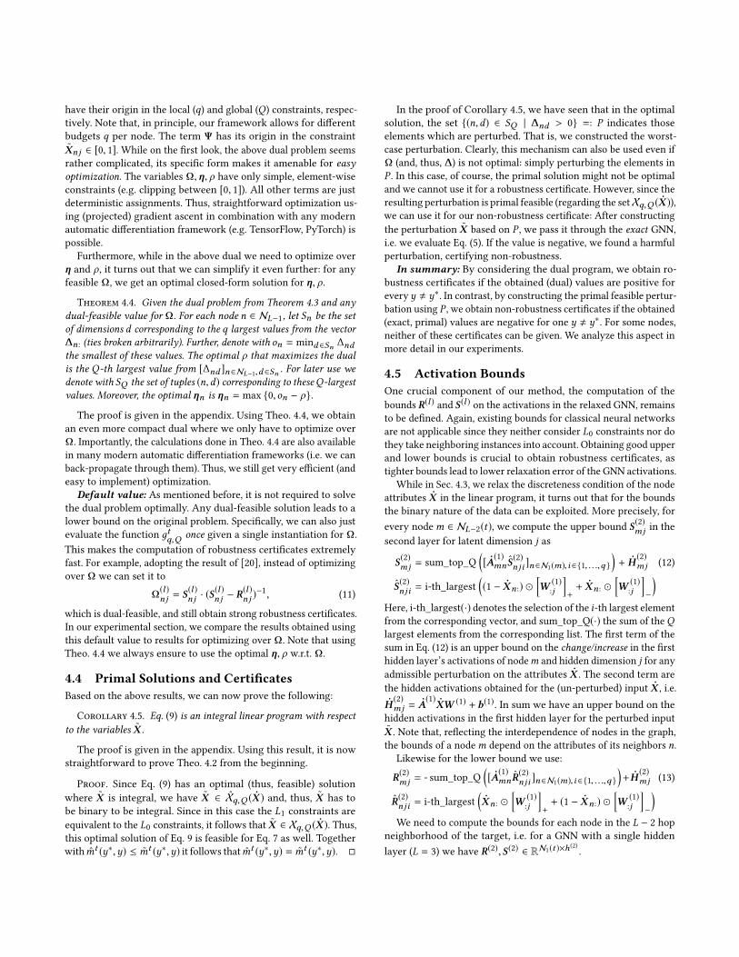
Figure 1: Certificates for a GNN trained

with standard training on Cora-ML.

0.0 0.2 0.4 0.6 0.8 1.0

Nb. purity

0

25

50

75

100

Avg.MaxQrobust Mean

95% CI

Figure 2: Neighborhood purity cor-

relates with robustness.

21

23

25

27

Degree

0

25

50

75

100

Avg.MaxQrobust Mean

95% CI

Figure 3: Robustness of nodes vs.

their degree.

where yt = argmaxk f tθ ( ÛX , ÛA)k is the predicted label for node t .Note again that the unlabeled nodes are used for robustness pur-

poses only – making it very different to the principle of self-training

(see below). Overall, Eq. (18) aims to correctly classify all labeled

nodes using the exact GNN, while making sure that every node has

at least a margin of M∗ from the decision boundary even under

worst-case perturbations.Eq. (18) can be optimized as is. In practice, however, we proceed

as follows:We first train the GNN on the labeled nodes using Eq. (17)until convergence. Then we train on all nodes using Eq. (18) untilconvergence.

Discussion: Note that the above idea is not applicable to the

robust cross entropy loss from Eq. (15). One might argue that one

could use a GNN trained using Eq. (15) to compute predictions for

all (or some of the) unlabeled nodes. Then, treating these predictions

as the correct (soft-)labels for the nodes and recursively apply the

training. This has two undesired effects: If the prediction is very

uncertain (i.e. the soft-labels are flat), Eq. (15) tries to find a GNN

where the worst-case margin exactly matches these uncertain labels

(since this minimizes the cross-entropy). The GNN will be forced to

keep the prediction uncertain for such instances even if it could do

better. On the other hand, if the prediction is very certain (i.e. very

peaky), Eq. (15) tries to make sure that even in the worst-case the

prediction has such high certainty – thus being overconfident in the

prediction (which might even be wrong in the first place). Indeed,

this case mimics the idea of self-training: In self-training, we first

train our model on the labeled nodes. Subsequently, we use the

predicted classes of (some of) the unlabeled nodes, pretending these

are their true labels; and continue training with them as well. Self-

training, however, serves an orthogonal purpose and, in principle,

can be used with any of the above models.

Summary:When training the GNN, the lower and upper activa-

tion bounds are treated as a function of θ , i.e. they are updated ac-

cordingly. While this can be done efficiently as discussed in Sec. 4.5,

it is still the least efficient part of our model and future work might

consider incremental computations. Overall, since the dual pro-

gram in Theorem 4.3 and the upper/lower activations bounds are

differentiable, we can train a robust GNN with gradient descent

and standard deep learning libraries. Note again that by setting Ωto its default value, we actually only have to optimize over θ – like

in standard training. Furthermore, computing ptθ for the default

parameters has roughly the same cost as evaluating a usual (sliced)

GNN K many times, i.e. it is very efficient.

6 EXPERIMENTAL EVALUATION

Our experimental contributions are twofold. (i) We evaluate the

robustness of traditionally trained GNNs using, and thus analyz-

ing, our certification method. (ii) We show that our robust training

procedure can dramatically improve GNNs’ robustness while sacri-

ficing only minimal accuracy on the unlabeled nodes.

We evaluate our method on the widely used and publicly avail-

able datasets Cora-ML (N=2,995, E=8,416, D=2,879, K=7) [16], Cite-

seer (N=3,312, E=4,715, D=3,703, K=6) [19], and PubMed (N=19,717,

E=44,324, D=500, K=3) [19]. For every dataset, we allow local (i.e.per-node) changes to the node attributes amounting to 1% of the

attribute dimension, i.e. q = 0.01D. Q is analyzed in detail in the

experiments reflecting different perturbation spaces.

We refer to the traditional training of GNNs as Cross Entropy(short CE), to the robust variant of cross entropy as Robust CrossEntropy (RCE), and to our hinge loss variants as Robust Hinge Loss(RH) and Robust Hinge Loss with Unlabeled (RH-U), where the latterenforces a margin loss also on the unlabeled nodes. We set M1,

i.e. the margin on the training nodes to log(0.9/0.1) and M2 to

log(0.6/0.4) for the unlabeled nodes (RH-U only). This means that

we train the GNN to (correctly) classify the labeled nodes with

output probability of 90% in the worst case, and the unlabeled nodeswith 60%, reflecting that we do not want our model to be overcon-

fident on the unlabeled nodes. Please note that we do not need to

compare against graph adversarial attack models such as [21] since

our method gives provable guarantees on the robustness.

While our method can be used for any GNN of the form in

Eq. (1), we study the well-established GCN [12], which has shown

to outperform many more complicated models. Following [12], we

consider GCNs with one hidden layer (i.e. L = 3), and choose a

latent dimensionality of 32. We split the datasets into 10% labeled

and 90% unlabeled nodes. See the appendix for further details.

6.1 Certificates: Robustness of GNNs

We first start to investigate our (non-)robustness certificates by ana-

lyzing GNNs trained using standard cross entropy training. Figure 1

shows the main result: for varying Q we report the percentage of

nodes (train+test) which are certifiable robust/non-robust on Cora-

ML. We can make two important observations: (i) Our certificates

are often very tight. That is, the white area (nodes for which we

cannot give any – robustness or non-robustness – certificate) is

rather small. Indeed, for any givenQ , at most 30% of the nodes can-

not be certified across all datasets and despite no robust training,

0 50 100 15012

Certificate w.r.t Q

0

50

100

%Nodes

Certifiably

robust

Certifiably

nonrobust

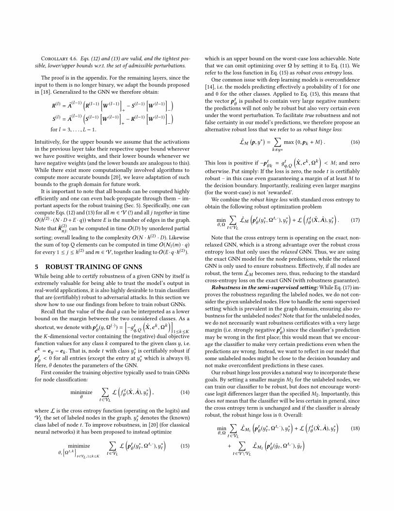
Figure 4: Robust training (Cora-ML).

Dashed lines are w/o robust training.

0 50 10012

Certificate w.r.t Q

0

50

100

%Nodes

Certifiably

robust

Certifiably

nonrobust

Figure 5: Robust training (Citeseer).

Dashed lines are w/o robust training.

0 50 10012

Certificate w.r.t Q

0

50

100

%Nodescert.robust

RH-U

RCE

RH

CE

Figure 6: RH-U is most successful for

robustness at Q = 12 (Cora-ML).

highlighting the tightness of our bounds and relaxations and the

effectiveness of our certification method. (ii) GNNs trained tradi-

tionally are only certifiably robust up to very small perturbations.

At Q = 12, less than 55% of the nodes are certifiably robust on

Cora-ML. In case of Citeseer even less than 20% (Table 1; training:

CE). Even worse, at this point already two thirds (for Citeseer) anda quarter (Cora-ML) of the nodes are certifiably non-robust (i.e. we

can find adversarial examples), confirming the issues reported in

[21]. PubMed behaves similarly (as we will see later, e.g., in Table 1).

In our experiments, the labeled nodes are on average more robust

than the unlabeled nodes, which is not surprising given that the

classifier was not trained using the labels of the latter.

We also investigate what contributes to certain nodes being more

robust than others. In Figure 2 we see that neighborhood purity (i.e.

the share of nodes in a respective node’s two-hop neighborhood

that is assigned the same class by the classifier) plays an important

role. OnCora-ML, almost all nodes that are certifiably robust aboveQ ≥ 50 have a neighborhood purity of at least 80%. When analyzing

the degree (Figure 3), it seems that nodes with a medium degree are

most robust. While counterintuitive at first, having many neighbors

also means a large surface for adversarial attacks. Nodes with low

degree, in contrast, might be affected more strongly since each node

in its neighborhood has a larger influence.

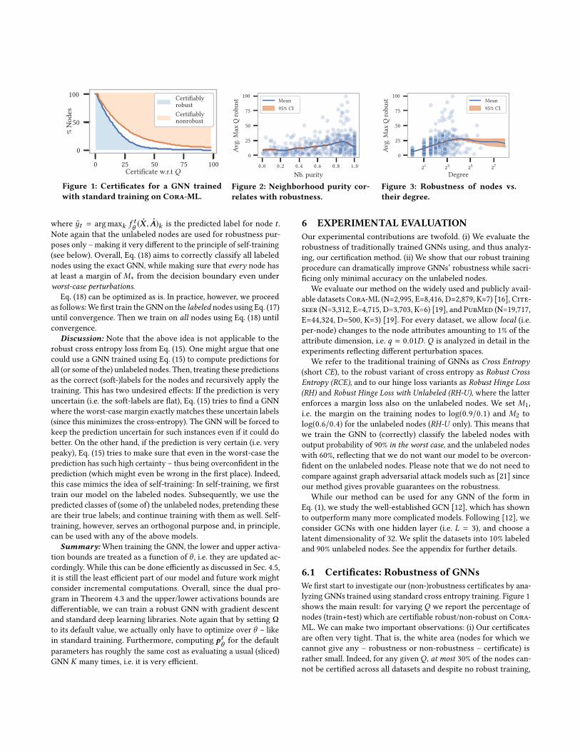
0 5 10Dual-Primal Difference

Den

sity

Ω opt.

Default Ω

Figure 7: Difference of

Primal andDual Bound.

Tightness of lower bounds:Next, we aim to analyze how tight

our dual lower bounds are, which

we needed to obtain efficient cer-

tification. For this, we analyze

(i) the value of дq,Q (·) we ob-

tain from our dual solution (either

when optimizing overΩ are using

the default value), compared to (ii)

the value of the primal solution

we obtain using our construction

from Sec. 4.4. The smaller the difference, the better. As seen in

Figure 7, when optimizing over Ω, for most of the nodes the gap is

0. Thus, indeed we can often find the exact minimum of the primal

via the dual. As expected, when using the default value for Ω the

difference between dual and primal is larger. Still, for most nodes

the difference is small. Indeed, and more importantly, when consid-

ering the actual certificates (where we only need to verify whether

the dual is positive; its actual value is not important), the difference

between optimizing Ω and its default value become negligible: on

Cora-ML, the average maximal Q for which we can certify robust-

ness drops by 0.54; Citeseer 0.18; PubMed 2.3. This highlights that

we can use the default values of Ω to very efficiently certify many

or even all nodes in a GNN. In all remaining experiments we, thus,

only operate with this default choice.

6.2 Robust Training of GNNs

Next, we analyze our robust training procedure. If not mentioned

otherwise, we use our robust hinge-loss including the unlabeled

nodes RH-U and we robustify the models with Q = 12 since for

this value more than 50% of nodes across our datasets were not

certifiably robust (when using standard training).

Figure 4 and 5 show again the percentage of certified nodes

w.r.t. a certain Q – now when using a robustly trained GCN. With

dotted lines, we have plotted the curves one obtains for the standard

(non-robust) training – e.g. the dotted lines in Fig. 4 are the ones

already seen in Fig. 1. As it becomes clear, with robust training, we

can dramatically increase the number of nodes which are robust.

Almost every node is robust when considering the Q for which

the model has been trained for. E.g. for Citeseer, our method is

able to quadruple the number of certifiable nodes for Q = 12. Put

simply: When performing an adversarial attack withQ ≤ 12 on this

model, it cannot do any harm! Moreover the share of nodes that

can be certified for any given Q has increased significantly (even

thoughwe have not trained themodel forQ > 12). Most remarkably,

nodes for which we certified non-robustness before become now

certifiably robust (the blue region above the gray lines).

Accuracy: The increased robustness comes at almost no loss inclassification accuracy as Table 1 shows. There we report the results

for all datasets and all training principles. The last two columns

show the accuracy obtained for node classification (for train and

test nodes separately). In some cases, our robust classifiers even

outperform the non-robust one on the unlabeled nodes. Interest-

ingly, for PubMed we see that the accuracy on the labeled nodes

drops to the accuracy on the unlabeled nodes. This indicates that

our method can even improve generalization.

Training principles: Comparing the different robust training

procedures (also given in more detail in Figure 6), we see that RH-U

achieves significantly higher robustness when considering Q = 12.

This is shown by the third-last column in the table, where the

percentage of nodes which are certifiably robust forQ = 12 (i.e. the

Q the models have been robustified for) is shown. The third column

shows the largest Q for which a node is still certifiably robust

(averaged over all nodes). As shown, for all training principles the

average exceeds the value of 12.

Effect of training with Q : If we strongly increase the Q for

which the classifier is trained for, we only observe a small drop in

Dataset Training

Avg. Max

Q robust

% Robust

Q = 12

Acc.

(labeled)

Acc.

(unlabeled)

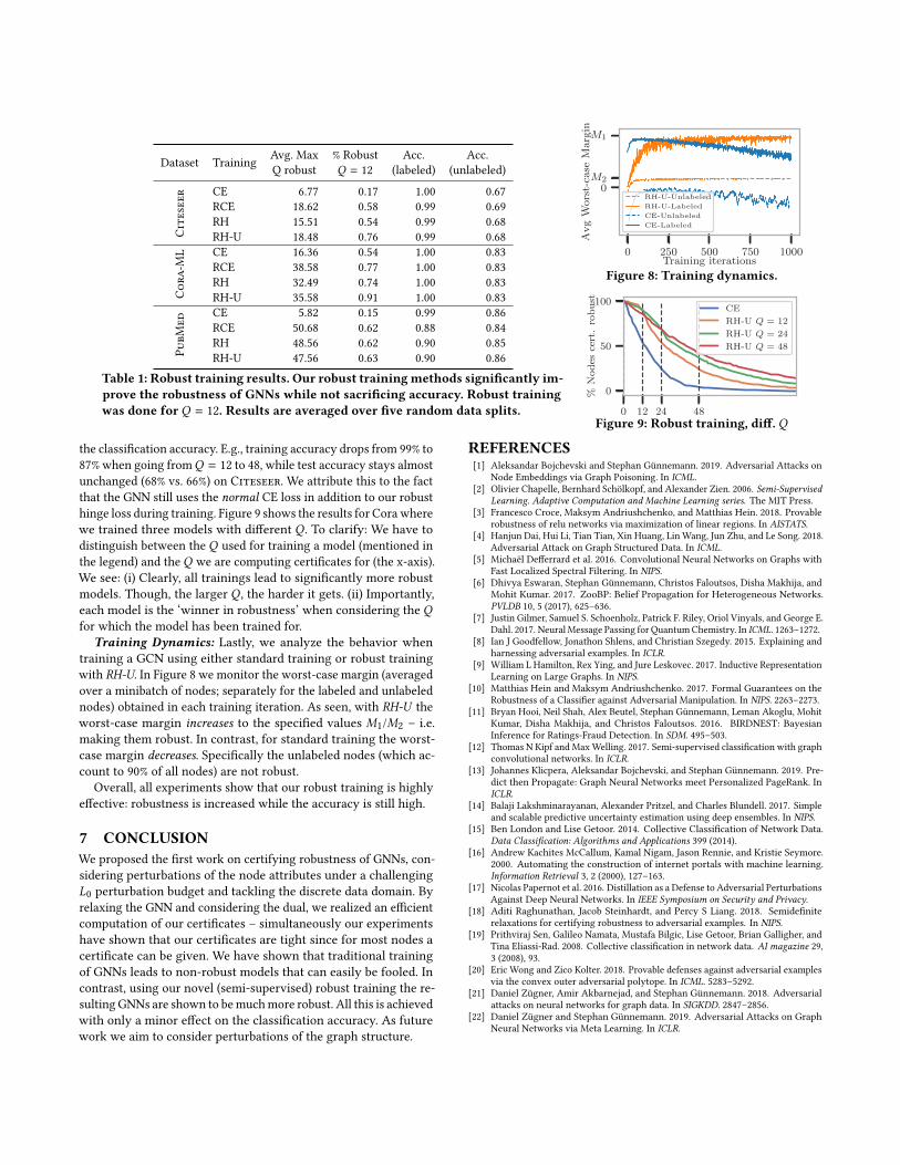
Citeseer CE 6.77 0.17 1.00 0.67

RCE 18.62 0.58 0.99 0.69

RH 15.51 0.54 0.99 0.68

RH-U 18.48 0.76 0.99 0.68

Cora-ML CE 16.36 0.54 1.00 0.83

RCE 38.58 0.77 1.00 0.83

RH 32.49 0.74 1.00 0.83

RH-U 35.58 0.91 1.00 0.83

PubMed

CE 5.82 0.15 0.99 0.86

RCE 50.68 0.62 0.88 0.84

RH 48.56 0.62 0.90 0.85

RH-U 47.56 0.63 0.90 0.86

Table 1: Robust training results. Our robust trainingmethods significantly im-

prove the robustness of GNNs while not sacrificing accuracy. Robust training

was done for Q = 12. Results are averaged over five random data splits.

0 250 500 750 1000Training iterations

0M2

M1

Avg

Wors

t-ca

seM

arg

in

RH-U-Unlabeled

RH-U-Labeled

CE-Unlabeled

CE-Labeled

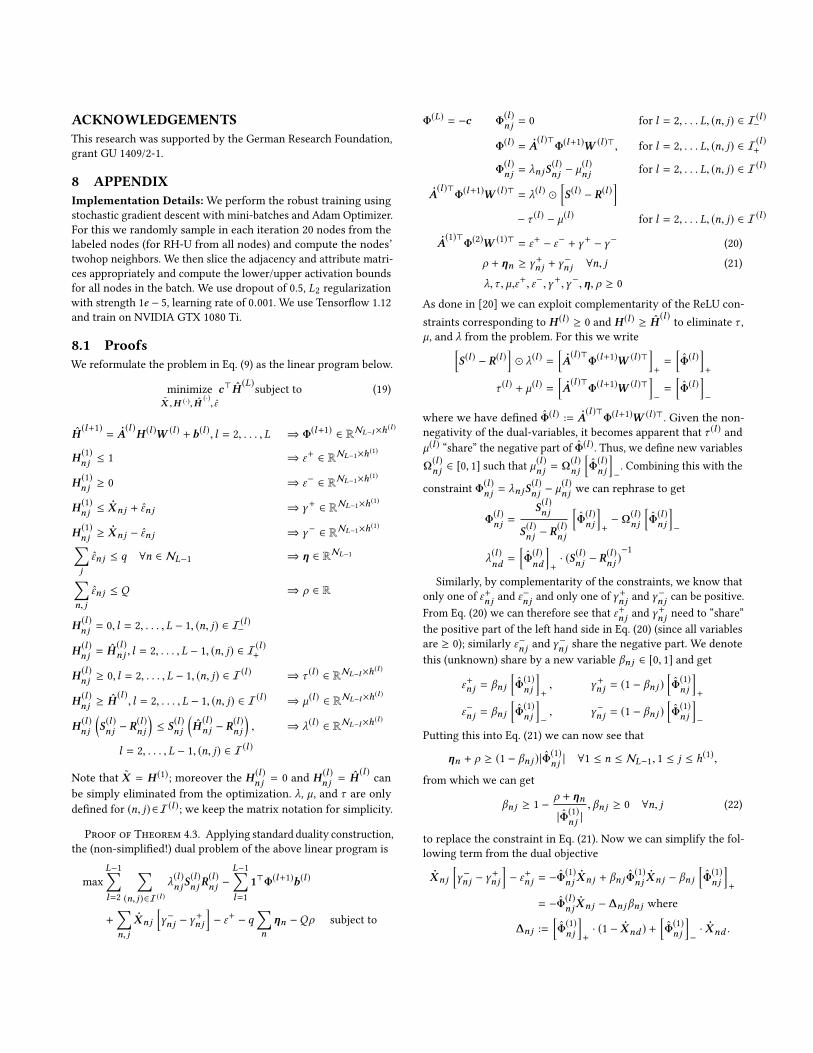
Figure 8: Training dynamics.

0 12 24 48

0

50

100

%N

od

esce

rt.

rob

ust

CE

RH-U Q = 12

RH-U Q = 24

RH-U Q = 48

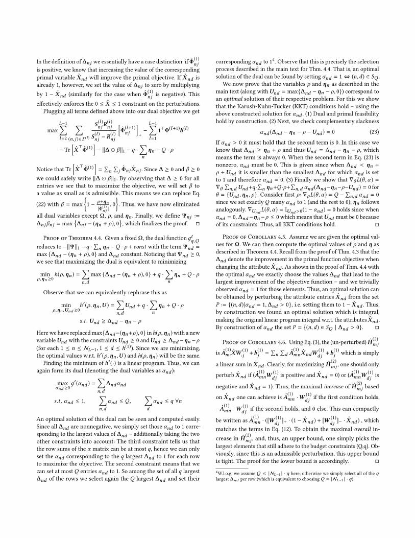
Figure 9: Robust training, diff. Q

the classification accuracy. E.g., training accuracy drops from 99% to

87% when going fromQ = 12 to 48, while test accuracy stays almost

unchanged (68% vs. 66%) on Citeseer. We attribute this to the fact

that the GNN still uses the normal CE loss in addition to our robust

hinge loss during training. Figure 9 shows the results for Corawhere

we trained three models with different Q . To clarify: We have to

distinguish between the Q used for training a model (mentioned in

the legend) and theQ we are computing certificates for (the x-axis).

We see: (i) Clearly, all trainings lead to significantly more robust

models. Though, the larger Q , the harder it gets. (ii) Importantly,

each model is the ‘winner in robustness’ when considering the Qfor which the model has been trained for.

Training Dynamics: Lastly, we analyze the behavior when

training a GCN using either standard training or robust training

with RH-U. In Figure 8 we monitor the worst-case margin (averaged

over a minibatch of nodes; separately for the labeled and unlabeled

nodes) obtained in each training iteration. As seen, with RH-U the

worst-case margin increases to the specified values M1/M2 – i.e.

making them robust. In contrast, for standard training the worst-

case margin decreases. Specifically the unlabeled nodes (which ac-

count to 90% of all nodes) are not robust.

Overall, all experiments show that our robust training is highly

effective: robustness is increased while the accuracy is still high.

7 CONCLUSION

We proposed the first work on certifying robustness of GNNs, con-

sidering perturbations of the node attributes under a challenging

L0 perturbation budget and tackling the discrete data domain. By

relaxing the GNN and considering the dual, we realized an efficient

computation of our certificates – simultaneously our experiments

have shown that our certificates are tight since for most nodes a

certificate can be given. We have shown that traditional training

of GNNs leads to non-robust models that can easily be fooled. In

contrast, using our novel (semi-supervised) robust training the re-

sulting GNNs are shown to bemuchmore robust. All this is achieved

with only a minor effect on the classification accuracy. As future

work we aim to consider perturbations of the graph structure.

REFERENCES

[1] Aleksandar Bojchevski and Stephan Günnemann. 2019. Adversarial Attacks on

Node Embeddings via Graph Poisoning. In ICML.[2] Olivier Chapelle, Bernhard Schölkopf, and Alexander Zien. 2006. Semi-Supervised

Learning. Adaptive Computation and Machine Learning series. The MIT Press.

[3] Francesco Croce, Maksym Andriushchenko, and Matthias Hein. 2018. Provable

robustness of relu networks via maximization of linear regions. In AISTATS.[4] Hanjun Dai, Hui Li, Tian Tian, Xin Huang, Lin Wang, Jun Zhu, and Le Song. 2018.

Adversarial Attack on Graph Structured Data. In ICML.[5] Michaël Defferrard et al. 2016. Convolutional Neural Networks on Graphs with

Fast Localized Spectral Filtering. In NIPS.[6] Dhivya Eswaran, Stephan Günnemann, Christos Faloutsos, Disha Makhija, and

Mohit Kumar. 2017. ZooBP: Belief Propagation for Heterogeneous Networks.

PVLDB 10, 5 (2017), 625–636.

[7] Justin Gilmer, Samuel S. Schoenholz, Patrick F. Riley, Oriol Vinyals, and George E.

Dahl. 2017. Neural Message Passing for QuantumChemistry. In ICML. 1263–1272.[8] Ian J Goodfellow, Jonathon Shlens, and Christian Szegedy. 2015. Explaining and

harnessing adversarial examples. In ICLR.[9] William L Hamilton, Rex Ying, and Jure Leskovec. 2017. Inductive Representation

Learning on Large Graphs. In NIPS.[10] Matthias Hein and Maksym Andriushchenko. 2017. Formal Guarantees on the

Robustness of a Classifier against Adversarial Manipulation. In NIPS. 2263–2273.[11] Bryan Hooi, Neil Shah, Alex Beutel, Stephan Günnemann, Leman Akoglu, Mohit

Kumar, Disha Makhija, and Christos Faloutsos. 2016. BIRDNEST: Bayesian

Inference for Ratings-Fraud Detection. In SDM. 495–503.

[12] Thomas N Kipf and MaxWelling. 2017. Semi-supervised classification with graph

convolutional networks. In ICLR.[13] Johannes Klicpera, Aleksandar Bojchevski, and Stephan Günnemann. 2019. Pre-

dict then Propagate: Graph Neural Networks meet Personalized PageRank. In

ICLR.[14] Balaji Lakshminarayanan, Alexander Pritzel, and Charles Blundell. 2017. Simple

and scalable predictive uncertainty estimation using deep ensembles. In NIPS.[15] Ben London and Lise Getoor. 2014. Collective Classification of Network Data.

Data Classification: Algorithms and Applications 399 (2014).[16] Andrew Kachites McCallum, Kamal Nigam, Jason Rennie, and Kristie Seymore.

2000. Automating the construction of internet portals with machine learning.

Information Retrieval 3, 2 (2000), 127–163.[17] Nicolas Papernot et al. 2016. Distillation as a Defense to Adversarial Perturbations

Against Deep Neural Networks. In IEEE Symposium on Security and Privacy.[18] Aditi Raghunathan, Jacob Steinhardt, and Percy S Liang. 2018. Semidefinite

relaxations for certifying robustness to adversarial examples. In NIPS.[19] Prithviraj Sen, Galileo Namata, Mustafa Bilgic, Lise Getoor, Brian Galligher, and

Tina Eliassi-Rad. 2008. Collective classification in network data. AI magazine 29,3 (2008), 93.

[20] Eric Wong and Zico Kolter. 2018. Provable defenses against adversarial examples

via the convex outer adversarial polytope. In ICML. 5283–5292.[21] Daniel Zügner, Amir Akbarnejad, and Stephan Günnemann. 2018. Adversarial

attacks on neural networks for graph data. In SIGKDD. 2847–2856.[22] Daniel Zügner and Stephan Günnemann. 2019. Adversarial Attacks on Graph

Neural Networks via Meta Learning. In ICLR.

ACKNOWLEDGEMENTS

This research was supported by the German Research Foundation,

grant GU 1409/2-1.

8 APPENDIX

Implementation Details:We perform the robust training using

stochastic gradient descent with mini-batches and Adam Optimizer.

For this we randomly sample in each iteration 20 nodes from the

labeled nodes (for RH-U from all nodes) and compute the nodes’

twohop neighbors. We then slice the adjacency and attribute matri-

ces appropriately and compute the lower/upper activation bounds

for all nodes in the batch. We use dropout of 0.5, L2 regularizationwith strength 1e − 5, learning rate of 0.001. We use Tensorflow 1.12

and train on NVIDIA GTX 1080 Ti.

8.1 Proofs

We reformulate the problem in Eq. (9) as the linear program below.

minimize

˜X ,H (·),H(·), εc⊤H

(L)subject to (19)

H(l+1)

= ÛA(l )H (l )W (l ) + b(l ), l = 2, . . . ,L ⇒ Φ(l+1) ∈ RNL−l×h(l )

H (1)nj ≤ 1 ⇒ ε+ ∈ RNL−1×h(1)

H (1)nj ≥ 0 ⇒ ε− ∈ RNL−1×h(1)

H (1)nj ≤ ÛXnj + εnj ⇒ γ+ ∈ RNL−1×h(1)

H (1)nj ≥ ÛXnj − εnj ⇒ γ− ∈ RNL−1×h(1)∑jεnj ≤ q ∀n ∈ NL−1 ⇒ η ∈ RNL−1∑

n, jεnj ≤ Q ⇒ ρ ∈ R

H (l )nj = 0, l = 2, . . . ,L − 1, (n, j) ∈ I(l )

−

H (l )nj = H

(l )nj , l = 2, . . . ,L − 1, (n, j) ∈ I(l )

+

H (l )nj ≥ 0, l = 2, . . . ,L − 1, (n, j) ∈ I(l ) ⇒ τ (l ) ∈ RNL−l×h(l )

H (l )nj ≥ H

(l ), l = 2, . . . ,L − 1, (n, j) ∈ I(l ) ⇒ µ(l ) ∈ RNL−l×h(l )

H (l )nj

(S(l )nj − R(l )nj

)≤ S(l )nj

(H

(l )nj − R(l )nj

), ⇒ λ(l ) ∈ RNL−l×h(l )

l = 2, . . . ,L − 1, (n, j) ∈ I(l )

Note that˜X = H (1)

; moreover the H (l )nj = 0 and H (l )

nj = H(l )

can

be simply eliminated from the optimization. λ, µ, and τ are only

defined for (n, j) ∈I(l ); we keep the matrix notation for simplicity.

Proof of Theorem 4.3. Applying standard duality construction,

the (non-simplified!) dual problem of the above linear program is

max

L−1∑l=2

∑(n, j)∈I(l )

λ(l )njS

(l )njR

(l )nj −

L−1∑l=1

1⊤Φ(l+1)b(l )

+∑n, j

ÛXnj

[γ−nj − γ+nj

]− ε+ − q

∑n

ηn −Qρ subject to

Φ(L) = −c Φ(l )nj = 0 for l = 2, . . . L, (n, j) ∈ I(l )

−

Φ(l ) = ÛA(l )⊤Φ(l+1)W (l )⊤, for l = 2, . . . L, (n, j) ∈ I(l )

+

Φ(l )nj = λnjS

(l )nj − µ

(l )nj for l = 2, . . . L, (n, j) ∈ I(l )

ÛA(l )⊤Φ(l+1)W (l )⊤ = λ(l ) ⊙

[S(l ) − R(l )

]− τ (l ) − µ(l ) for l = 2, . . . L, (n, j) ∈ I(l )

ÛA(1)⊤Φ(2)W (1)⊤ = ε+ − ε− + γ+ − γ− (20)

ρ + ηn ≥ γ+nj + γ−nj ∀n, j (21)

λ,τ , µ,ε+, ε−,γ+,γ−,η, ρ ≥ 0

As done in [20] we can exploit complementarity of the ReLU con-

straints corresponding to H (l ) ≥ 0 and H (l ) ≥ H(l )

to eliminate τ ,µ, and λ from the problem. For this we write[

S(l ) − R(l )]⊙ λ(l ) =

[ÛA(l )⊤

Φ(l+1)W (l )⊤]+=

[ˆΦ(l )

]+

τ (l ) + µ(l ) =[ÛA(l )⊤

Φ(l+1)W (l )⊤]−=

[ˆΦ(l )

]−

where we have definedˆΦ(l )

:= ÛA(l )⊤Φ(l+1)W (l )⊤

. Given the non-

negativity of the dual-variables, it becomes apparent that τ (l ) andµ(l ) “share” the negative part of ˆΦ(l )

. Thus, we define new variables

Ω(l )nj ∈ [0, 1] such that µ

(l )nj = Ω(l )

nj

[ˆΦ(l )nj

]−. Combining this with the

constraint Φ(l )nj = λnjS

(l )nj − µ

(l )nj we can rephrase to get

Φ(l )nj =

S(l )nj

S(l )nj − R(l )nj

[ˆΦ(l )nj

]+− Ω(l )

nj

[ˆΦ(l )nj

]−

λ(l )nd =

[ˆΦ(l )nd

]+· (S(l )nj − R(l )nj )

−1

Similarly, by complementarity of the constraints, we know that

only one of ε+nj and ε−nj and only one of γ+nj and γ

−nj can be positive.

From Eq. (20) we can therefore see that ε+nj and γ+nj need to “share”

the positive part of the left hand side in Eq. (20) (since all variables

are ≥ 0); similarly ε−nj and γ−nj share the negative part. We denote

this (unknown) share by a new variable βnj ∈ [0, 1] and get

ε+nj = βnj[ˆΦ(1)nj

]+, γ+nj = (1 − βnj )

[ˆΦ(1)nj

]+

ε−nj = βnj[ˆΦ(1)nj

]−, γ−nj = (1 − βnj )

[ˆΦ(1)nj

]−

Putting this into Eq. (21) we can now see that

ηn + ρ ≥ (1 − βnj )| ˆΦ(1)nj | ∀1 ≤ n ≤ NL−1, 1 ≤ j ≤ h(1),

from which we can get

βnj ≥ 1 − ρ + ηn

| ˆΦ(1)nj |, βnj ≥ 0 ∀n, j (22)

to replace the constraint in Eq. (21). Now we can simplify the fol-

lowing term from the dual objective

ÛXnj

[γ−nj − γ+nj

]− ε+nj = − ˆΦ(1)

njÛXnj + βnj ˆΦ

(1)nj

ÛXnj − βnj[ˆΦ(1)nj

]+

= − ˆΦ(l )nj

ÛXnj − ∆njβnj where

∆nj :=[ˆΦ(1)nj

]+· (1 − ÛXnd ) +

[ˆΦ(1)nj

]−· ÛXnd .

In the definition of∆nj we essentially have a case distinction: if ˆΦ(1)nj

is positive, we know that increasing the value of the corresponding

primal variable˜Xnd will improve the primal objective. If

ÛXnd is

already 1, however, we set the value of ∆nj to zero by multiplying

by 1 − ÛXnd (similarly for the case whenˆΦ(1)nj is negative). This

effectively enforces the 0 ≤ ˜X ≤ 1 constraint on the perturbations.

Plugging all terms defined above into our dual objective we get

max

L−1∑l=2

∑(n, j)∈I(l )

S(l )njR(l )nj

S(l )nj − R(l )nj

[ˆΦ(l+1)nj

]+−L−1∑l=1

1⊤Φ(l+1)b(l )

− Tr

[ÛX⊤

ˆΦ(1)]− ∥∆ ⊙ β ∥1 − q ·

∑n

ηn −Q · ρ

Notice that Tr

[ÛX⊤

ˆΦ(1)]=∑n∑j ˆΦnj ÛXnj . Since ∆ ≥ 0 and β ≥ 0

we could safely write ∥∆ ⊙ β ∥1. By observing that ∆ ≥ 0 for all

entries we see that to maximize the objective, we will set β to

a value as small as is admissible. This means we can replace Eq.

(22) with β = max

1 − ρ+ηn

| ˆΦ(1)nj |, 0

. Thus, we have now eliminated

all dual variables except Ω, ρ, and ηn . Finally, we define Ψnj :=

∆njβnj = max

∆nj − (ηn + ρ), 0

, which finalizes the proof.

Proof of Theorem 4.4. Given a fixed Ω, the dual function дtq,Qreduces to −∥Ψ∥1 − q ·∑n ηn −Q · ρ + const with the term Ψnd =

max ∆nd − (ηn + ρ), 0 and ∆nd constant. Noticing that Ψnd ≥ 0,

we see that maximizing the dual is equivalent to minimizing

min

ρ,ηn ≥0h(ρ,ηn ) =

∑n,d

max ∆nd − (ηn + ρ), 0 + q ·∑n

ηn +Q · ρ

Observe that we can equivalently rephrase this as

min

ρ,ηn,Und ≥0h′(ρ,ηn ,U ) =

∑n,d

Und + q ·∑n

ηn +Q · ρ

s .t . Und ≥ ∆nd − ηn − ρ

Herewe have replacedmax∆nd−(ηn+ρ), 0 inh(ρ,ηn )with a newvariableUnd with the constraintsUnd ≥ 0 andUnd ≥ ∆nd −ηn −ρ

(for each 1 ≤ n ≤ NL−1, 1 ≤ d ≤ h(1)). Since we are minimizing,

the optimal values w.r.t. h′(ρ,ηn ,U ) and h(ρ,ηn ) will be the same.

Finding the minimum of h′(·) is a linear program. Thus, we can

again form its dual (denoting the dual variables as αnd ):

max

αnd ≥0д′(αnd ) =

∑n,d

∆ndαnd

s .t . αnd ≤ 1,∑n,d

αnd ≤ Q,∑d

αnd ≤ q ∀n

An optimal solution of this dual can be seen and computed easily.

Since all ∆nd are nonnegative, we simply set those αnd to 1 corre-

sponding to the largest values of ∆nd – additionally taking the two

other constraints into account: The third constraint tells us that

the row sums of the α matrix can be at most q, hence we can only

set the αnd corresponding to the q largest ∆nd to 1 for each row

to maximize the objective. The second constraint means that we

can set at most Q entries αnd to 1. So among the set of all q largest

∆nd of the rows we select again the Q largest ∆nd and set their

corresponding αnd to 14. Observe that this is precisely the selection

process described in the main text for Thm. 4.4. That is, an optimal

solution of the dual can be found by setting αnd = 1 ⇔ (n,d) ∈ SQ .

We now prove that the variables ρ and ηn as described in the

main text (along withUnd = max∆nd −ηn − ρ, 0) correspond to

an optimal solution of their respective problem. For this we show

that the Karush-Kuhn-Tucker (KKT) conditions hold – using the

above constructed solution for αnd . (1) Dual and primal feasibility

hold by construction. (2) Next, we check complementary slackness

αnd (∆nd − ηn − ρ −Und ) = 0 (23)

If αnd > 0 it must hold that the second term is 0. In this case we

know that ∆nd ≥ ηn + ρ and thus Und = ∆nd − ηn − ρ, whichmeans the term is always 0. When the second term in Eq. (23) is

nonzero, αnd must be 0. This is given since when ∆nd < ηn +ρ +Und it is smaller than the smallest ∆nd for which αnd is set

to 1 and therefore αnd = 0. (3) Finally we show that ∇θL(θ ,α) =∇θ

∑n,d Und+q·

∑n ηn+Q ·ρ+∑n,d αnd (∆nd−ηn−ρ−Und ) = 0 for

θ = Und ,ηn , ρ. Consider first ρ: ∇ρL(θ ,α) = Q −∑n,d αnd = 0

since we set exactlyQ many αnd to 1 (and the rest to 0); ηn follows

analogously. ∇Und L(θ ,α) = IUnd>0(1 − αnd ) = 0 holds since when

αnd = 0,∆nd −ηn−ρ ≤ 0which means thatUnd must be 0 because

of its constraints. Thus, all KKT conditions hold.

Proof of Corollary 4.5. Assume we are given the optimal val-

ues for Ω. We can then compute the optimal values of ρ and η as

described in Theorem 4.4. Recall from the proof of Thm. 4.3 that the

∆nd denote the improvement in the primal function objective when

changing the attributeÛXnd . As shown in the proof of Thm. 4.4 with

the optimal αnd we exactly choose the values ∆nd that lead to the

largest improvement of the objective function – and we trivially

observed αnd = 1 for those elements. Thus, an optimal solution can

be obtained by perturbing the attribute entriesÛXnd from the set

P := (n,d)|αnd = 1,∆nd > 0, i.e. setting them to 1 − ÛXnd . Thus,

by construction we found an optimal solution which is integral,

making the original linear program integral w.r.t. the attributes˜Xnd .

By construction of αnd the set P = (n,d) ∈ SQ | ∆nd > 0.

Proof of Corollary 4.6. Using Eq. (3), the (un-perturbed) H(2)mj

isÛA(1)m:

ÛXW (1):j +b

(1)j =

∑n∑d ÛA(1)

mn ÛXndW(1)d j +b

(1)j which is simply

a linear sum inÛXnd . Clearly, for maximizing H

(2)mj , one should only

perturbÛXnd if (

ÛA(1)mnW

(1)d j is positive and

ÛXnd = 0) or (ÛA(1)mnW

(1)d j is

negative andÛXnd = 1). Thus, the maximal increase of H (2)

mj based

onÛXnd one can achieve is

ÛA(1)mn ·W (1)

d j if the first condition holds,

− ÛA(1)mn ·W (1)

d j if the second holds, and 0 else. This can compactly

be written asÛA(1)mn · ([W (1)

d j ]+ · (1 − ÛXnd ) + [W(1)d j ]− · ÛXnd ) , which

matches the terms in Eq. (12). To obtain the maximal overall in-

crease in H(2)mj , and, thus, an upper bound, one simply picks the

largest elements that still adhere to the budget constraints (Q,q). Ob-

viously, since this is an admissible perturbation, this upper bound

is tight. The proof for the lower bound is accordingly.

4W.l.o.g. we assume Q ≤ |NL−1 | · q here; otherwise we simply select all of the qlargest ∆nd per row (which is equivalent to choosing Q = |NL−1 | · q)