certification report for srm 2214: density of iso-octane
TRANSCRIPT
NIST Special Publication 260-186
Standard Reference Materials®
Certification Report for SRM 2214: Density of Iso-octane for Extended
Ranges of Temperature and Pressure
Mark O. McLinden Jolene Splett
This publication is available free of charge from: https://doi.org/10.6028/NIST.SP.260-186

NIST Special Publication 260-186
Standard Reference Materials®
Certification Report for SRM 2214: Density of Iso-octane for Extended
Ranges of Temperature and Pressure
Mark O. McLinden Applied Chemicals and Materials Division
Materials Measurement Laboratory
Jolene Splett Statistical Engineering Division
Information Technology Laboratory
This publication is available free of charge from: https://doi.org/10.6028/NIST.SP.260-186
October 2016
U.S. Department of Commerce Penny Pritzker, Secretary
National Institute of Standards and Technology Willie May, Under Secretary of Commerce for Standards and Technology and Director

Certain commercial entities, equipment, or materials may be identified in this document in order to describe an experimental procedure or concept adequately.
Such identification is not intended to imply recommendation or endorsement by the National Institute of Standards and Technology, nor is it intended to imply that the entities, materials, or equipment are necessarily the best available for the purpose.
National Institute of Standards and Technology Special Publication 260-186 Natl. Inst. Stand. Technol. Spec. Publ. 260-186, 38 pages (October 2016)
CODEN: NSPUE2
This publication is available free of charge from: https://doi.org/10.6028/NIST.SP.260-186

Abstract
______________________________________________________________________________________________________ This publication is available free of charge from
: https://doi.org/10.6028/NIS
T.SP
.260-186
This report of analysis documents procedures used to obtain certified values and associated uncertainties of the density of iso-octane SRM 2214 over an extended range of temperatures and pressures. This SRM is certified over the temperature range –50˚C to 160˚C and pressure range of 0.1 MPa to 30 MPa; an interpolation model is provided to calculate the density within these ranges. This SRM has a density of 691.853 kg⋅m–3 at t = 20˚C and p = 0.1 MPa. The certification measurements were carried out in a two-sinker magnetic-suspension densimeter. The SRM material is commercial, high-purity iso-octane (2,2,4-trimethylpentane, CAS 540-84-1). Measurements were made on both degassed material and material saturated with nitrogen, and an estimated correction surface (valid over the range –50˚C ≤ t ≤ 100˚C and 0.1 MPa ≤ p ≤ 20 MPa) gives the density difference between the nitrogen-saturated and degassed materials. A thorough analysis of the uncertainties is presented; this includes effects resulting from the experimental density determination, possible degradation of the sample due to time and exposure to high temperatures, dissolved air, uncertainties in the empirical density model, and the sample-to-sample variations in the SRM vials. Also considered is the effect of uncertainties in the user’s temperature and pressure measurements. This SRM is intended for the calibration of industrial densimeters.
Keywords Standard reference material; iso-octane; density; measurement
i

Table of Contents
______________________________________________________________________________________________________ This publication is available free of charge from
: https://doi.org/10.6028/NIS
T.SP
.260-186
Abstract .................................................................................................................................. i 1. Introduction .............................................................................................................................. 1 2. Experimental Methodology ..................................................................................................... 2
2.1 Densimeter ....................................................................................................................... 2 2.2 Experimental material ...................................................................................................... 3 2.3 Density measurement procedures .................................................................................... 3
3. Results for Fluid Density ......................................................................................................... 5 4. Uncertainty Evaluation ............................................................................................................ 8
4.1 Fluid density, ρ, and its uncertainty, u(ρ) ....................................................................... 8 4.2 Air-saturation, Δ, and its uncertainty, u(Δ) ...................................................................... 9 4.3 Vial-to-vial uncertainty, u(V) ......................................................................................... 11 4.4 Uncertainty due to material degradation, u(x) ............................................................... 11 4.5 Uncertainty due to user’s temperature and pressure errors, u(tp) ................................. 13 4.6 Uncertainty due to the apparatus, u(e) .......................................................................... 14
4.6.1 Weighings, W1, W2, Wcal, Wtare ............................................................................. 14 4.6.2 Density of Nitrogen, ρΝ2 ...................................................................................... 15 4.6.3 Drift Correction, ρ0 .............................................................................................. 15 4.6.4 Mass of Sinkers, mx .............................................................................................. 16
4.6.4.1 Balance Readings, O1, O2, O3, O4 ............................................................... 17 4.6.4.2 Calibration Data for Standard Masses ......................................................... 17 4.6.4.3 Density of air, ρair ....................................................................................... 18 4.6.4.4 Density ρx, and mass mx of sinkers .............................................................. 19
4.6.5 Sinker Volumes ..................................................................................................... 19 4.6.5.1 Sinker volume, V1, V2 at reference conditions ............................................. 19 4.6.5.2 Sinker volume, V1, V2 as a f (t, p) ................................................................. 20 4.6.5.3 Sinker volume, Vcal, Vtare .............................................................................. 23
4.6.6 Summary of u(ρfluid) .............................................................................................. 23 5. Summary of Uncertainties ..................................................................................................... 26
5.1 Combined Standard Uncertainty .................................................................................... 26 5.2 Expanded Uncertainty and Degrees of Freedom ........................................................... 26
6. Discussion and Conclusions .................................................................................................. 28 References .................................................................................................................................. 29 APPENDIX—Measured Values of Iso-octane Fluid Density ................................................... 30
ii

List of Tables
______________________________________________________________________________________________________ This publication is available free of charge from
: https://doi.org/10.6028/NIS
T.SP
.260-186
Table 1. Estimated parameters for the density model given in Eq. 2 .......................................... 6 Table 2. Estimated fluid density ! in kg⋅m–3 for degassed samples from Eq. 2 .......................... 7 Table 3. Vial-to-vial uncertainty ................................................................................................ 11 Table 4. Estimated uncertainty due to user’s temperature and pressure uncertainties .............. 13 Table 5. Uncertainties due to systematic and random effects for the density of nitrogen ......... 15 Table 6. Sequence of vacuum and iso-octane measurements .................................................... 15 Table 7. Calibration data for standard masses ........................................................................... 17 Table 8. Estimated density and the associated uncertainty for each sinker ............................... 19 Table 9. Estimated mass and the associated uncertainty, "($%), for each sinker ..................... 19 Table 10. Systematic errors associated with V1,ref and V2,ref ...................................................... 20
Table 11. Uncertainty budgets for V1,ref and V2,ref ........................................................................ 20 Table 12. Constants for volume correction factors .................................................................... 22 Table 13. Uncertainty budget for !fluid at 30 ˚C and 1 MPa ...................................................... 24 Table 14. Uncertainty budget for !fluid at 160 ˚C and 30 MPa .................................................. 25 Table 15. Percentages of total variation in u(ρfluid) for six sources of uncertainty .................... 25 Table 16. Combined standard uncertainty in ρc ........................................................................ 27 Table A1. Experimentally measured temperatures t, pressures p, and densities ρexp,
for degassed SRM iso-octane .................................................................................... 30 Table A2. Experimentally measured temperatures t, pressures p, and densities ρexp,
for nitrogen-saturated SRM iso-octane ..................................................................... 36
List of Figures
Figure 1. Degassed density measurements versus temperature and pressure .............................. 5 Figure 2. Residuals of the density interpolation model (Eq. 2) from the measured
data versus temperature ................................................................................................ 9 Figure 3. Density correction for air-saturated versus degassed iso-octane based on
experimentally measured points ................................................................................ 10 Figure 4. Estimated correction surface for air-saturated versus degassed iso-octane (Eq. 8) ... 11 Figure 5. Replicate measurements at 30 ˚C for various samples of iso-octane ......................... 12 Figure 6. Residuals from the polynomial fit of data at T = 30 ˚C .............................................. 13 Figure 7. Values of !' for five vacuum data sets over time ...................................................... 16 Figure 8. Sinker volume adjustment (eq. 25) as a function of temperature ............................... 23
iii

______________________________________________________________________________________________________ This publication is available free of charge from
: https://doi.org/10.6028/NIS
T.SP
.260-186
1. Introduction This document describes the measurement procedures and analyses used to characterize the uncertainty associated with the density of liquid iso-octane (SRM 2214) for a wide range of temperatures and pressures.
The property of fluid density is a vital parameter in a multitude of industrial processes. These include the control of chemical processes and the metering of fuels and other commodity chemicals. Often, the process stream is sampled through an industrial densimeter for continuous, real-time determination of the density. Such densimeters are not absolute instruments—they must be regularly calibrated at the conditions of use with fluids of known density. The work presented here utilizes an absolute fluid densimeter to establish the density of iso-octane as a function of temperature and pressure for use as a calibration standard.
Iso-octane (formal IUPAC name 2,2,4-trimethylpentane, with CAS registry number 540-84-1) has a number of advantages as a density standard: it is a stable chemical of relatively low toxicity; its density of 692 kg⋅m–3 at ambient conditions is well matched to many applications, particularly liquid hydrocarbon fuels; its freezing point of –107˚C and boiling point of 99˚C cover the range of many industrial processes. Iso-octane has low surface tension compared to that of water, and it is relatively inexpensive. The National Institute of Standards and Technology (NIST) has sold a density Standard Reference Material (SRM®) based on iso-octane since 2001, but the previous SRM was certified only at ambient conditions: 15˚C to 25˚C and normal atmospheric pressure.
This SRM certifies the density of a particular batch of iso-octane. This approach is preferred for high-accuracy calibrations over the alternative approach of measuring the density of “very pure” iso-octane for at least two reasons. First, a batch certification is directly traceable to NIST, and this is often a requirement for high-level calibration laboratories. Second, iso-octane in very high purities is difficult to obtain. Impurities, such as closely related organic compounds, are often present. The use of “pure” iso-octane would greatly complicate the traceability of density and shift the problem to one of determining purity and/or the effects of impurities on the density.
In section 2, we briefly summarize the experimental methodology used to generate density measurements. Section 3 describes an empirical model used to estimate fluid density for various temperatures and pressures, and section 4 provides details regarding the uncertainty evaluation for the density values. Combined standard uncertainties and expanded uncertainties are summarized in section 5. Finally, a brief discussion and conclusions are given in section 6.
1

______________________________________________________________________________________________________ This publication is available free of charge from
: https://doi.org/10.6028/NIS
T.SP
.260-186
2. Experimental Methodology
2.1 Densimeter
The two-sinker densimeter used in this work is described in detail by McLinden and Lösch-Will [1] and McLinden and Splett [2], and this general type of instrument is described by Wagner and Kleinrahm [3]. In the present densimeter, two sinkers of nearly the same mass, surface area, and surface material, but very different volumes, are weighed separately with a high-precision balance while immersed in a fluid of unknown density. The fluid density ρ is given by
(m1 − m2 ) − (W1 − W2 )ρ = , (1)(V1 − V2 )
where m and V are the sinker mass and volume, W is the balance reading, and the subscripts refer to the two sinkers. The main advantage of the two-sinker method is that adsorption onto the surface of the sinkers, systematic errors in the weighing, and other effects that reduce the accuracy of most buoyancy techniques cancel. Equation (1) must be corrected for magnetic effects; this is considered in Section 4 and described in detail by McLinden et al. [4].
A magnetic suspension coupling transmits the gravity and buoyancy forces on the sinkers to the balance, thus isolating the fluid sample (which may be at high pressure and/or extremes of temperature) from the balance. The central elements of the coupling are two magnets, one on each side of a nonmagnetic pressure separating wall. The top magnet, which is an electromagnet with a ferrite core, is hung from the balance. The bottom (permanent) magnet is held in stable suspension with respect to the top magnet by means of a feedback control circuit making fine adjustments in the electromagnet current. The permanent magnet is linked with a lifting device to pick up a sinker for weighing. A mass comparator with a resolution of 1 µg and a capacity of 111 g is used for the weighings. Each sinker has a mass of 60 g; one is made of tantalum and the other is titanium.
In addition to the sinkers, suspension coupling, and balance that comprise the density measuring system, the apparatus included a thermostat, pressure instrumentation, and a sample handling system. The temperature was measured with a standard-reference-quality platinum resistance thermometer (SPRT) and resistance bridge referenced to a thermostatted standard resistor. The signal from the SPRT was used directly in a digital control circuit to maintain the cell temperature constant within ±0.001 K. The pressures were measured with state-of-the-art transducers combined with careful calibration. The transducers (as well as the pressure manifold) were thermostatted to minimize the effects of variations in laboratory temperature.
The thermostat served to isolate the measuring cell from ambient conditions. It was a vacuum-insulated, cryostat-type design. The measuring cell was surrounded by an isothermal shield, which thermally isolated it from variations in ambient temperature; this shield was maintained at a constant (±0.01 K) temperature 1 K below the cell temperature. Electric heaters compensated for the small heat flow from the cell to the shield and allowed millikelvin-level control of the cell
2

______________________________________________________________________________________________________ This publication is available free of charge from
: https://doi.org/10.6028/NIS
T.SP
.260-186
temperature. Operation at sub-ambient temperatures was effected by circulating ethanol from an external chiller through channels in the shield.
2.2 Experimental material
The material used is identical to the previous SRM, which was obtained from a commercial source.[5] The SRM is provided in 5 mL flame-sealed glass ampoules. At the same time the 5 mL ampoules were prepared, several large 1.5 L flame-sealed ampoules were also prepared containing the same iso-octane. We worked with material from one of the 1.5 L ampoules, except for some of the chemical analysis, which used the 5 mL ampoules. We transferred the iso-octane from the 1.5 L ampoule to a stainless-steel sample cylinder for convenience in sample handling.
The sample was degassed by freezing the stainless-steel cylinder in liquid nitrogen, evacuating the vapor space, and thawing. This freeze/pump/thaw process was repeated a total of eleven times. The residual pressure over the frozen sample on the final cycle was 0.001 Pa. The SRM as supplied by NIST contains some amount of dissolved air. The sample was degassed to obtain a well characterized state for the measurements. Also, we were concerned that dissolved air could react with the iso-octane at the elevated temperatures measured in this work. We felt that the uncertainties introduced by “purifying” the SRM material in this way would be offset by a reduction in possible effects resulting from reaction with air.
To quantify the effect of dissolved air on the density, additional measurements were made on a sample that was saturated with nitrogen at a temperature of 20 ˚C and pressure of 0.10 MPa. A quantity of the degassed iso-octane was transferred to an evacuated 500 mL stainless steel sample cylinder. Ultra-high-purity nitrogen (99.9995 %) was admitted to the cylinder to a pressure of 0.10 MPa; additional nitrogen was admitted periodically over the course of five days to maintain the pressure at 0.10 MPa. The cylinder was periodically mixed to promote equilibrium. This point is discussed further in Section 4.2.
A chemical analysis by gas chromatography-mass spectrometry yielded an overall purity of 99.72 %. The major impurities, totaling 0.20 %, were isomers of dimethylpentane. In addition, 2,3-dimethylbutane was present at 0.058 % and 2-methylbutane was present at 0.017 %. Two additional peaks at the level of 0.001 % could not be identified.
2.3 Density measurement procedures
Each density determination involved weighings in the order: tantalum (Ta) sinker, titanium (Ti) sinker, balance calibration weight, balance tare weight, balance tare weight (again), balance calibration weight, Ti sinker, and Ta sinker, for a total of eight weighings—two for each object. For each weighing, the balance was read six times over the course of ten seconds. For each object, the 12 balance readings were averaged for the calculation of density. Between each of the object weighings, and also before the first weighing and following the final weighing, the temperature and pressure were recorded, for a total of nine readings of t and p; these were also averaged. A complete density determination required 12 minutes. The weighing design was
3

______________________________________________________________________________________________________ This publication is available free of charge from
: https://doi.org/10.6028/NIS
T.SP
.260-186
symmetrical with respect to time, and this tended to cancel the effects of any drift in the temperature or pressure.
The sample was loaded at a low temperature and pressure. Higher pressures were generated by heating the liquid-filled cell; thus avoiding the need for any type of compressor, which could have been a source of contamination. Starting at the lowest temperature and pressure for a given filling, measurements were made at increasing temperatures (and nearly constant density) until the maximum desired pressure was reached. The sample was then vented to a lower pressure along an isotherm.
The densimeter control program monitored the system temperatures and pressures once every 60 seconds. A running average and standard deviation of the temperatures and pressures were computed for the preceding eight readings. When these were within preset tolerances of the set point conditions, a weighing sequence was triggered. Once the specified number of replicate density determinations were made at a given (t, p) state point, the control program then moved to the next temperature or automatically vented the sample to the next pressure on an isotherm.
A total of three separate fillings of the densimeter were carried out with the degassed sample. The first two covered the entire range of temperature and pressure. Following the measurements at high temperatures and high pressures with the first two fillings, the densimeter was cooled to 30˚C and a small quantity of fresh sample was added to refill the cell; replicate measurements were performed to check for possible degradation. These tests are discussed in Section 4.4. The third filling extended over the temperature range of –59˚C to 62˚C. A fourth filling was carried out with the nitrogen-saturated sample; it extended over the full range of temperature and pressure.
Between each filling, and also before the first filling and following the last filling, the system was evacuated and the density recorded multiple times. The indicated density was used to determine the apparatus zero ρ0. The value of ρ0 used in the density calculation is the time-weighted average of ρ0 values measured before and after a given density determination (see Section 4.6.3).
4

______________________________________________________________________________________________________ This publication is available free of charge from
: https://doi.org/10.6028/NIS
T.SP
.260-186
3. Results for Fluid Density The density of iso-octane was measured over the temperature range –59˚C to 160˚C, with pressures ranging from 0.5 MPa to 30 MPa. The measured values are tabulated in the Appendix, and a plot of the densities measured on the degassed sample is shown in Figure 1.
Figure 1. Degassed density measurements versus temperature and pressure.
An empirical model for interpolation was fit to the degassed density data
ˆ 2 a + c ⋅ ln T e ⋅ p + g ⋅ ⎡⎣ln T ⎤⎦ + i ⋅ p2 + k ⋅ p ⋅ ln T( ) + ˆ ( ) ( ) ρ = f T , p( ) = 2 + ε , (2)
1+ b ⋅ ln T ⎡⎣ ( ) ⎤⎦ ( ) ( ) + d ⋅ p + f ⋅ ln T + h ⋅ p2 + j ⋅ p ⋅ ln T
where T is temperature in kelvins (T/K = t/˚C + 273.15) and p is pressure in MPa. The estimated model parameters are listed in Table 1. Table 2 gives estimated fluid density values calculated with Eq. 2 at even temperature and pressure increments.
5

Table 1. Estimated parameters for the density model given in Eq. 2.
______________________________________________________________________________________________________ This publication is available free of charge from
: https://doi.org/10.6028/NIS
T.SP
.260-186
( 1.022794253⋅103
) -2.832862261⋅10–1
* -3.049340500⋅102
+ 2.565415217⋅10–3
, 2.724090192⋅100
- 1.985515546⋅10–2
. 2.265907341⋅101
ℎ 1.768055678⋅10–6
0 1.685280491⋅10–3
1 -3.255136085⋅10–4
2 -3.866274772⋅10–1
6

______________________________________________________________________________________________________ This publication is available free of charge from
: https://doi.org/10.6028/NIS
T.SP
.260-186
Table 2. Estimated fluid density ρ in kg⋅m–3 for degassed samples (Δ = g = 0 kg⋅m–3) from Eq. 2.
t (˚C) Pressure (MPa)
0.1 1 2 5 10 15 20 25 30 -50 747.992 748.564 749.194 751.049 754.033 756.895 759.647 762.299 764.859 -40 740.081 740.690 741.360 743.330 746.494 749.522 752.428 755.225 757.923 -30 732.159 732.807 733.520 735.616 738.972 742.177 745.248 748.198 751.039 -20 724.213 724.905 725.666 727.896 731.460 734.854 738.098 741.209 744.200 -10 716.232 716.972 717.784 720.162 723.949 727.545 730.973 734.253 737.402 0 708.204 708.996 709.865 712.403 716.432 720.243 723.866 727.325 730.638 10 700.116 700.966 701.896 704.610 708.900 712.942 716.773 720.420 723.905 20 691.956 692.869 693.868 696.774 701.347 705.637 709.687 713.532 717.199 30 683.709 684.693 685.767 688.884 693.765 698.320 702.604 706.659 710.515 40 675.361 676.423 677.582 680.930 686.146 690.987 695.520 699.796 703.850 50 666.896 668.046 669.298 672.902 678.484 683.632 688.431 692.939 697.202 60 658.297 659.545 660.900 664.789 670.770 676.250 681.331 686.086 690.567 70 649.543 650.902 652.374 656.578 662.997 668.835 674.218 679.233 683.942 80 640.614 642.097 643.700 648.257 655.156 661.381 667.086 672.377 677.326 90 631.484 633.109 634.860 639.810 647.239 653.884 659.934 665.515 670.716 100 623.911 625.830 631.223 639.237 646.337 652.756 658.645 664.111 110 614.476 616.586 622.478 631.140 638.735 645.549 651.765 657.507 120 604.768 607.098 613.556 622.937 631.072 638.309 644.872 650.905 130 594.749 597.332 604.433 614.617 623.341 631.034 637.963 644.302 140 584.372 587.248 595.086 606.168 615.535 623.718 631.037 637.696 150 573.582 576.799 585.484 597.575 607.649 616.359 624.091 631.087 160 562.310 565.929 575.594 588.823 599.674 608.953 617.124 624.474
7

______________________________________________________________________________________________________ This publication is available free of charge from
: https://doi.org/10.6028/NIS
T.SP
.260-186
4. Uncertainty Evaluation The overall uncertainty in the fluid density arises from several distinct sources. The first source is the empirical model (i.e., Eq. 2) used to represent the density and allow interpolation at a desired temperature and pressure. A second category relates to the material itself; these include uncertainties associated with the degree of air saturation of the iso-octane and possible degradation resulting from exposure to high temperatures. Since the SRM is provided in 5 mL ampoules (vials), the variation in density from vial to vial must also be considered. The third, and most complex, source arises from the experimental measurement of the density. Finally, when using the SRM for the calibration of a densimeter, the uncertainty in the user’s temperature and pressure measurement must be included.
The uncertainty evaluation described in this document closely follows the procedures outlined in [2]; please refer to that document for further details. The measurement equation used to estimate the density of iso-octane, ρc, is
ρc = ρ + Δ + V + x + e + tp , (3)
where
ρ is the estimated fluid density based on an empirical model (Eq. 2), Δ is the effect due to air saturation, V is the effect due to differences between vials, x is the effect due to material degradation over time, e is the effect due to the apparatus (i.e., experimental uncertainty), and tp is the effect due to the user’s temperature and pressure measurements.
The combined standard uncertainty of ρc is
u2 0.5 u(ρc ⎡⎣ ρ Δ V x e tp ⎦ . (4)) = ( ) + u2 ( ) + u2 ( ) + u2 ( ) + u2 ( ) + u2 ( ) ⎤
The degrees of freedom associated with u(ρc) are computed using the Welch-Satterthwaite approximation.
The remainder of section 4 is devoted to defining and describing each individual uncertainty component.
4.1 Fluid density, !, and its uncertainty, "(!)
Fluid density values are computed using Eq. 2. The residuals of Eq. 2 from the measured data are shown in Figure 2. The root-mean-square-error (RMSE) of the fit was 0.010 kg⋅m–3. For any given temperature and pressure combination within the range of data, the value of u(ρ) is conservatively estimated to be 0.020 kg⋅m–3 based on 495 - 11 = 484 degrees of freedom
8

______________________________________________________________________________________________________ This publication is available free of charge from
: https://doi.org/10.6028/NIS
T.SP
.260-186
(dfρ = 484). Four points at T = 397.13 K and p = 0.98 MPa were removed from the analysis, as were data measured on the thermally-degraded sample (test numbers c8_1201a and c8_1202a).
Figure 2. Residuals of the density interpolation model (Eq. 2) from the measured data versus temperature.
4.2 Air-saturation, Δ, and its uncertainty, u(Δ)
The correction for air saturation is
Δ = Fair ⋅ g , (5)
where Fair is the fraction of air contained in the sample relative to a fully saturated sample, and g is the difference between density measurements of air-saturated and degassed samples (Figure 3). We assume here that nitrogen (which was measured) and air have the same effect on density. The proportion of air contained in the SRM is estimated to be between 0.57 and 0.77. Thus the uncertainty of Fair, based on a uniform distribution, is u(Fair) = 0.058 (dfFair = 8).
9

______________________________________________________________________________________________________ This publication is available free of charge from
: https://doi.org/10.6028/NIS
T.SP
.260-186
To estimate g, we first fitted rational functions to density measurements of the air-saturated and degassed samples separately. Temperatures higher than 390 K were not fitted.
a1 + a2 ln ( ) t + a3 p + a4 ⎡⎣ln ( ) t ⎤⎦ 2 + a6 p
2 + a7 p ln ( ) tρsaturated = 2 (6)
1+ a8 ln ( ) t + a9 p + a10 ⎡⎣ln t + a11 p2 + a12 p ln ( ) t( ) ⎤⎦
b1 + b2 ln ( ) t + b3 p + b4 ⎡⎣ln t 2 + b6 p
2 + b7 p ln t( ) ⎤⎦ ( ) ρdegassed = 2 (7)
1+ b8 ln t ln t ( ) ( ) + b9 p + b10 ⎡⎣ ( ) ⎤⎦ + b11 p2 + b12 p ln t
Next, we computed % = ( −(degassed and fit a planar model based on temperature and saturated pressure to the computed g values (as shown in Figure 4):
g = −0.1323697352 − 0.0004029095 ⋅ t + 0.0039491677 ⋅ p − 0.0000356174 ⋅ t ⋅ p , (8)
where the limits are t = –50 ˚C to 100 ˚C, and p = 0.1 MPa to 20 MPa.
The uncertainty of g is estimated as the worst-case prediction error associated with the planar model, u(g) = 0.020 kg⋅m–3 (dfg = 563 – 4 = 559). The uncertainty of the correction for air-saturation, Δ, is
2 ⋅u2 0.5 u Δ ⎡⎣g
2 ⋅u2 (Fair ) + Fair ( ) ⎤⎦ (9)( ) = g .
For example, u(Δ) = 0.0156 kg⋅m–3 for the SRM sample at t = 20˚C and p = 0.1 MPa with Fair = 0.67 (with u(Fair) defined above) and u(g) = 0.020 kg⋅m–3 .
Figure 3. Density correction for air-saturated versus degassed iso-octane based on experimentally measured points.
10
______________________________________________________________________________________________________ This publication is available free of charge from
: https://doi.org/10.6028/NIS
T.SP
.260-186
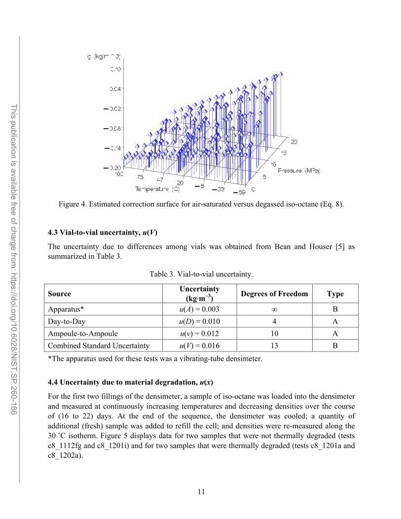
Figure 4. Estimated correction surface for air-saturated versus degassed iso-octane (Eq. 8).
4.3 Vial-to-vial uncertainty, u(V)
The uncertainty due to differences among vials was obtained from Bean and Houser [5] as summarized in Table 3.
Table 3. Vial-to-vial uncertainty.
Source Uncertainty (kg⋅m–3) Degrees of Freedom Type
Apparatus* u(A) = 0.003 ∞ B Day-to-Day u(D) = 0.010 4 A Ampoule-to-Ampoule u(v) = 0.012 10 A Combined Standard Uncertainty u(V) = 0.016 13 B *The apparatus used for these tests was a vibrating-tube densimeter.
4.4 Uncertainty due to material degradation, u(x)
For the first two fillings of the densimeter, a sample of iso-octane was loaded into the densimeter and measured at continuously increasing temperatures and decreasing densities over the course of (16 to 22) days. At the end of the sequence, the densimeter was cooled; a quantity of additional (fresh) sample was added to refill the cell; and densities were re-measured along the 30 ˚C isotherm. Figure 5 displays data for two samples that were not thermally degraded (tests c8_1112fg and c8_1201i) and for two samples that were thermally degraded (tests c8_1201a and c8_1202a).
11

______________________________________________________________________________________________________ This publication is available free of charge from
: https://doi.org/10.6028/NIS
T.SP
.260-186
To quantify material degradation, we fit a 4th order polynomial to the 30°C isotherm for samples that were not thermally degraded and examined residuals for the thermally degraded samples (see Figure 6). The largest absolute residual (0.024 kg⋅m–3) represents the worst-case error that might be observed. Thus, residuals from the fit are bounded by 0 and 0.024 kg⋅m–3. Assuming that these bounds represent limits to a uniform distribution, then u(x) = 0.007 kg⋅m–3 (dfx = 42).
720(
710(
700(
690(
680(
Pressure (MPa) id c8_1112fg c8_1201a c8_1201i c8_1202a
Figure 5. Replicate measurements at 30 ˚C for various samples of iso-octane. Samples measured for tests c8_1112fg and c8_1201i were not thermally degraded; samples measured for tests
c8_1201a and c8_1202a were thermally degraded.
Den
sity
(kg/
m^3
)
0 10 20 30(
12
______________________________________________________________________________________________________ This publication is available free of charge from
: https://doi.org/10.6028/NIS
T.SP
.260-186
0.005
0.000
-0.005
-0.010
-0.015
-0.020
-0.025
Pressure (MPa) id c8_1112fg c8_1201a c8_1201i c8_1202a
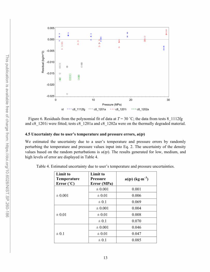
Figure 6. Residuals from the polynomial fit of data at T = 30 ˚C; the data from tests 8_1112fg and c8_1201i were fitted; tests c8_1201a and c8_1202a were on the thermally degraded material.
4.5 Uncertainty due to user’s temperature and pressure errors, u(tp)
We estimated the uncertainty due to a user’s temperature and pressure errors by randomly perturbing the temperature and pressure values input into Eq. 2. The uncertainty of the density values based on the random perturbations is u(tp). The results generated for low, medium, and high levels of error are displayed in Table 4.
Table 4. Estimated uncertainty due to user’s temperature and pressure uncertainties.
Res
idua
l (kg
/m^3
)
0 10 20 30
Limit to Temperature Error (˚C)
Limit to Pressure Error (MPa)
u(tp) (kg⋅m–3)
± 0.001 0.001 ± 0.001 ± 0.01 0.006
± 0.1 0.069 ± 0.001 0.004
± 0.01 ± 0.01 0.008 ± 0.1 0.070
± 0.001 0.046 ± 0.1 ± 0.01 0.047
± 0.1 0.085
13

______________________________________________________________________________________________________ This publication is available free of charge from
: https://doi.org/10.6028/NIS
T.SP
.260-186
The uncertainty values in the table are based on density surface boundaries of t = (–50 to 160) ˚C and p = (0.1 to 30) MPa. For our measurement system, u(tp) = 0.003 kg⋅m–3, based on u(t) = 0.002˚C and u(p) = 0.0025 kPa. We assume eight degrees of freedom (dftp = 8). These errors represent modeling errors and apply to the predicted ρ calculated using the rational function model (Eq. 2); they describe how the predicted ρ might be different for different levels of errors in temperature and pressure.
4.6 Uncertainty due to the apparatus, u(e)
The uncertainty due to the measurement apparatus is the uncertainty predicted using a polynomial equation fitted to the uncertainty in the fluid density. The equation for u(e) listed below was based on both saturated and degassed measurements.
u e( ) = u(ρf ) = f t( , p) = c1 + c2t + c3t2 + c4t
3 + c5t 3 + c6 p + c7 p
2 (10)luid
( ) = 4.249057 ×10⁻³ − 6.942 ×10⁻⁶ ⋅ t − 2.0376 ×10⁻⁸ ⋅ t 2 + 8.0679 ×10⁻¹¹ ⋅ t 3u e (11) +1.2451×10⁻¹³ ⋅ t 4 +1.64787 ×10⁻⁴ ⋅ p + 5.345 ×10⁻⁶ ⋅ p2
The measurement equation for ρfluid is
Wcal − Wtare α = (12)(mcal − mtare ) − ρN2 (Vcal − Vtare )
β = Wcal − (mcal − ρN2Vcal ) (13)α
⎡ m1 (W1 − W2 )⎤ ⎡ V1 (W1 − W2 )⎤ ⎢(V1 − V2 ) − ⎥ − ρ0
(14)ρfluid = ⎢(m1 − m2 ) − ⎥⎣ W1 −αβ ⎦ ⎣ W1 −αβ ⎦
The uncertainty of ρfluid is estimated using propagation of errors and the degrees of freedom are estimated using the Welch-Satterthwaite approximation. The remainder of section 4.6 describes the uncertainties required to compute u(ρfluid).
4.6.1 Weighings W1, W2, Wcal, Wtare
The recorded values of the sinker weighings W1, W2, Wcal, Wtare are averages of 12 measurements, so the uncertainty of a weighing, *(+,) is the standard deviation of the 12 readings divided by 12 (dfW1 = dfW2 = dfWcal = dfWtare = 11). Typical values of u(W1), u(W2), u(W3), and u(W4) are 1.48⋅10–6 g, 1.07⋅10–6 g, 2.65⋅10–6 g, and 2.51⋅10–6 g, respectively.
14

______________________________________________________________________________________________________ This publication is available free of charge from
: https://doi.org/10.6028/NIS
T.SP
.260-186
4.6.2 Density of Nitrogen, ρΝ2
We use the equation of state from [6] to estimate the density of nitrogen, which is used as a purge gas surrounding the balance, as a function of temperature and pressure. Propagation of errors is used to estimate the uncertainty of ρΝ2.
The uncertainties of temperature and pressure are comprised of uncertainties due to systematic and random effects that are added in quadrature. The values of the standard deviation in T and p, ST and Sp, are computed from nine repeat measurements.
Table 5. Uncertainties due to systematic and random effects for the density of nitrogen.
Source Uncertainty Due to Systematic Effects
Uncertainty due to Random Effects
Temperature 0.2 K (dfT = 8) /0
9 K (dfT = 8)
Pressure 2 ∙ 0.0001 kPa (dfp = 8) /6
9 kPa (dfp = 8)
4.6.3 Drift Correction, ρ0
The drift correction, ρ0, is estimated from “vacuum” data that was collected between fillings. Table 6 displays the sequence in which vacuum and iso-octane measurements were taken and Figure 7 shows the vacuum measurements.
Table 6. Sequence of vacuum and iso-octane measurements.
Dates Vacuum
Measurements Iso-octane
Filling 8 November 2011 – 16 November 2011 A
1 5 January 2012 – 8 January 2012 B
2 2 February 2012 – 3 February 2012 C
3 16 February 2012 – 17 February 2012 D
4 10 March 2012 – 12 March 2012 E
The drift correction was estimated by fitting a straight line to the vacuum data before and after an iso-octane filling. For example, a straight line was fit to vacuum data sets B and C to estimate ρ0
for the second iso-octane filling. To ensure data stability of the measurement system, we used the last 20 points in each measurement series for the analysis.
15

______________________________________________________________________________________________________ This publication is available free of charge from
: https://doi.org/10.6028/NIS
T.SP
.260-186
Rho
Zer
o (k
g/m
^3)
-0.0005
-0.0004
-0.0003
-0.0002
-0.0001
0.0000
0.0001
0.0002
0.0003
0.0004
0.0005
0.0006
0.0007
0 1000 2000 3000
Elapsed Time (h)
Vacuum Data Set A B C D E
Figure 7. Values of ( for five vacuum data sets over time.7
Thus, the drift correction, ρ0, for a straight line fit to adjacent pairs of vacuum data sets, is a function of the elapsed time, τ0,
( = 8 + 8 ; , (15)7 7 : 7
where 87 and 8: are fitting parameters. The uncertainty of ρ0 is
⎡ 1 )2 n
)2 ⎤∑(τ i −τ ⎥ , (16)u(ρ0 ) = s ⎢ + (τ 0 −τ n⎣ i=1 ⎦
where n is the number of observations used to estimate the regression parameters and s is the standard deviation of the fit. The degrees of freedom associated with the uncertainty estimate is n – 2. Values of ρ0 ranged from 2.12⋅10–5 kg⋅m–3 to 3.90⋅10–5 kg⋅m–3 .
4.6.4 Mass of Sinkers, mx
The mass of the density sinkers (m1 and m2) and calibration masses (mcal and mtare) were determined by a double-substitution weighing design as described by Harris and Torres [7]. A mass determination involved weighings of the unknown object mx (i.e., a sinker) and a standard mass ms, with each being weighed alone and together with a small “sensitivity mass” msw. Propagation of errors was used to estimate the uncertainty of a single mass determination using the measurement equation
16

______________________________________________________________________________________________________ This publication is available free of charge from
: https://doi.org/10.6028/NIS
T.SP
.260-186
⎧ ⎛ ⎞ ⎡ ⎤ ⎡ ⎛ ⎞ ⎤⎫ ⎛ ⎞⎪ ρair (O2 − O1 ) + (O3 − O4 ) ρair ⎪ ρairmx = ⎨ms 1− ⎠⎟ + ⎢ ⎥ ⎢msw 1− ⎥⎬ ⎠⎟
, (17)⎪ ⎝⎜ ρs ⎣ 2(O3 − O2 ) ⎦ ⎣ ⎝⎜ ρsw ⎠⎟ ⎦⎪ ⎝⎜
1−ρx⎩ ⎭
where
=:, =>, =?, and =@ represent balance readings, air is the density of ambient air during the mass determination,As and Asw are the standard masses,
and ( are the densities of the standard masses, ands sw
(
((, is the density of the object (e.g., sinker).
4.6.4.1 Balance Readings, O1, O2, O3, O4
The uncertainty of the balance reading was derived from the expanded uncertainty provided in the manufacturer’s instrument specifications:
0.00003 u O1 ) = u O2 ) = u O3 ) = u O4 ) = = 0.000015g . (18)( ( ( ( 2
4.6.4.2 Calibration Data for Standard Masses
Calibration data for the standard masses are listed in Table 7 as reported by the manufacturer of the standard masses.
Table 7. Calibration data for standard masses.
Nominal Mass (g)
Certified Mass (g)
Uncertainty (g)
Density (g⋅cm –3)
Uncertainty (g⋅cm –3)
50 50.000006 0.0000080 8.00 0.01545 20 20.000012 0.0000065 8.00 0.01545 20* 20.000009 0.0000065 8.00 0.01545 10 10.000010 0.0000050 8.00 0.01545 5 5.0000077 0.0000041 8.00 0.01545 2 2.0000050 0.00000305 8.00 0.01545
*one of the 20 g masses was distinguished by a small dimple
Nominal masses of (50 + 10) = 60 g and (20 + 20* + 5) = 45 g were used for As, and nominal masses of 5 g or 2 g were used for Asw. The nominal masses and their associated uncertainties were calculated as follows.
17

______________________________________________________________________________________________________
This publication is available free of charge from: https://doi.org/10.6028/N
IST.S
P.260-186
ms (60) = 50.000006 +10.000010 = 60.000016g
u m( s (60)) = ⎡(0.000008)2 + (0.000005)2 ⎤0.5
= 0.0000094g⎣ ⎦ ms (45) = 20.000012 + 20.000009 + 5.0000077 = 45.0000287g
u m( s (45)) = ⎡2 ⋅(0.0000065)2 + (0.0000041)2 ⎤0.5
= 0.0000101g⎣ ⎦ msw ( ) = 5.0000077g5
u msw 5 ) = 0.0000041g( ( ) msw ( ) = 2.0000050g2
u msw 2 ) = 0.00000305g( ( ) ρs = ρsw = 8.0g ⋅ cm-3
u(ρs ) = u(ρsw ) = 0.015g ⋅cm-3
4.6.4.3 Density of air, ρair
The density of air (in the balance chamber during the mass determinations) was computed with the CIPM 81/91 air density formula [8]:
pM a ⎛ Mv ⎞ρair = ⎢⎡1− xv ⎜1− ⎟ ⎥
⎤ (19)ZRT ⎝ M a ⎠⎣ ⎦
where
2 is pressure,B is thermodynamic temperature,CD is the mole fraction of water,EEF is the molar mass of dry air,D is the molar mass of water,
GH
is the compressibility factor, and is the molar gas constant.
Propagation of errors is used to compute the uncertainty of ρair using the following uncertainties for the thermometer, barometer, and hygrometer that were used to measure the atmospheric conditions:
u(T) = 0.2 K u(p) = 0.0001p/kPa u(h) = 0.02
Although the equation for ρair does not explicitly contain humidity, ℎ, CD is a function of ℎ.
18

______________________________________________________________________________________________________ This publication is available free of charge from
: https://doi.org/10.6028/NIS
T.SP
.260-186
4.6.4.4 Density !J, and mass mx, of sinkers
Sinker densities were computed from repeated measurements of volume and mass using the “hydrostatic comparator” described in [2] (for sinkers 1 and 2) and a simple hydrostatic experiment in water (for the cal and tare sinkers). The uncertainty was generated using the NIST Uncertainty Machine [9]. These values are given in Table 8.
Table 8. Estimated density and the associated uncertainty for each sinker.
Sinker Density (g⋅cm–3) Uncertainty (g⋅cm–3) Sinker 1 (Titanium) 4.511732 0.00000691 Sinker 2 (Tantalum) 16.663202 0.0000483 Cal 7.956976 0.0023 Tare 5.923001 0.0017
Between 6 and 12 mass determinations were completed for each sinker. Once the single mass determinations and their uncertainties were computed, they were combined using a random-effects model as described in section H.5.2 of [10]. Degrees of freedom are from the number of mass determinations for each sinker, k – 1. The final estimates of mass and their uncertainties for the four sinkers are listed in Table 9.
Table 9. Estimated mass and the associated uncertainty, *(A,), for each sinker.
Sinker Mass (g) Uncertainty (g) Degrees of Freedom Sinker 1 (Titanium) 60.075348 0.0000081 9 - 1 = 8 Sinker 2 (Tantalum) 60.055501 0.0000093 6 - 1 = 5 Cal 59.508634 0.0000067 12 - 1 = 11 Tare 44.296943 0.0000067 11 - 1 = 10
4.6.5 Sinker volumes
The volumes of the sinkers vary with temperature (thermal expansion) and pressure. They were calibrated at reference conditions, and the volume at the temperature and pressure of each density measurement was calculated with the correction terms described in the following sections.
4.6.5.1 Sinker volume, V1, V2 at reference conditions
The volumes of the sinkers were calibrated at t = 20˚C and p = 82 kPa by comparison to solid density standards of single-crystal silicon by use of a hydrostatic comparator as described by McLinden and Splett [2]. These “reference volumes” Vx,ref were 13.315363 cm3 for the titanium sinker (sinker “1”) and 3.604079 cm3 for the tantalum sinker (sinker “2”). This determination is subject to the systematic errors listed in Table 10, which were added in quadrature. The random
19

*
______________________________________________________________________________________________________ This publication is available free of charge from
: https://doi.org/10.6028/NIS
T.SP
.260-186
component is derived from a least-squares fit of ratios of sinker data from a designed experiment as described in [11]. The resulting uncertainties are given in Table 11. See [2] for further details.
Table 10. Systematic errors associated with V1,ref and V2,ref.
Source of Systematic Error Magnitude of Error Sinker 1 (Ti)
Uncertainty, cm3 Sinker 2 (Ta)
Uncertainty, cm3
Density of Standard 0.26⋅10–6 g/cm3 1.49⋅10–6 4.03⋅10–7
Mass of standard 5.0⋅10–5 g 0.29⋅10–5 0.803⋅10–5
Mass of object 5.0⋅10–5 g 3.07⋅10–5 3.07⋅10–5
Weighing of standard 5.0⋅10–5 g 0.96⋅10–5 0.26⋅10–5
Weighing of object 5.0⋅10–5 g 3.07⋅10–5 3.07⋅10–5
Table 11. Uncertainty budgets for V1,ref and V2,ref.
Source Sinker 1 (Ti) cm3 Sinker 2 (Ta) cm3
Systematic Component 4.46⋅10–5 cm3 (dfV1 = 8) 4.42⋅10–5 cm3 (dfV2 = 8) Random Component 1.54⋅10–5 cm3 (dfV1 = 6) 4.22⋅10–6 cm3 (dfV2 = 6) (K,, ref) 4.72⋅10–5 cm3 (dfV1 = 9) 4.44⋅10–5 cm3 (dfV2 = 8)
4.6.5.2 Sinker Volume, L , L as a f(t, p)M N
The volumes of the density sinkers will vary with the temperature and pressure of the fluid measurement, and thus the sinker volumes used to calculate density by Eq. (2) must be corrected. The volume of the sinkers is computed using
K, = K,,OPQ ∙ KR ∙ KS ∙ K0. (20)
The correction, KS, accounts for the decrease in volume with increased pressure; it is computed as
p − pref Vκ = 1− , (21)κ 0
where κ0 is the bulk modulus of elasticity of the sinker material, p is the fluid pressure in the densimeter and pref = 0.082 MPa. The uncertainty of the correction is
20

______________________________________________________________________________________________________ This publication is available free of charge from
: https://doi.org/10.6028/NIS
T.SP
.260-186
0.5 2⎡ ⎤ u Vκ ) = ⎜
p − pref u2 κ 0 )⎥ , (22)( ⎢⎛
2 ⎟⎞ (
⎢⎝ κ 0 ⎠ ⎥⎣ ⎦
where u(κ0) = κ0⋅0.05 and the uncertainties in p and pref are negligible (dfVκ = 8).
The KR term accounts for the change in sinker volume with temperature; it is given by
(1+1.0 ×10⁻⁶ ⋅Λ1 )3
Vα = . (23)(1+1.0 ×10⁻⁶ ⋅Λ2 )3
The value of KR for sinker 1 (titanium) is based on literature values for the coefficient of linear expansion reported by Touloukian [12], while the value for sinker 2 (tantalum) is based on data collected by Rubotherm Präzisionsmesstechnik, Germany. For sinker 1 (titanium):
Λ1 = 8.6538 ⋅T1 + 0.0048291⋅T12 −1.4220 ×10⁻⁵ ⋅T1
3 + 2.8263×10⁻⁸ ⋅T14
and
Λ2 = 8.6538 ⋅T2 + 0.0048291⋅T22 −1.4220 ×10⁻⁵ ⋅T2
3 + 2.8263 ×10⁻⁸ ⋅T24 ,
where T1 = T – 293.0 K, T2 = Tref – 293.0 K, and Tref = 293.15 K.
For sinker 2 (tantalum):
Λ1 = 0.0020336 + 5.9569 ⋅T1 − 0.00016957 ⋅T12 + 6.9633×10⁻⁶ ⋅T1
3
and
Λ2 = 0.0020336 + 5.9569 ⋅T2 − 0.00016957 ⋅T22 + 6.9633×10⁻⁶ ⋅T2
3 ,
where T1 = T – 300.738 K, T2 = Tref – 300.738 K, and Tref = 293.15 K.
The uncertainty of KR, *(KR), is included in *(K0) (see below) so uncertainty is not calculated for the Vα term.
A further correction for temperature effects (which was applied to both sinkers 1 and 2) is given by the VT term. This correction was based on argon measurements carried out over a range of pressures along a number of isotherms. The density measured for a temperature T and pressure p are ratioed to that measured for a reference temperature Tref (here Tref = 20.00 ˚C) at the same p; these density ratios are extrapolated to zero pressure where the ideal gas law applies. The VT term is based on the difference between the extrapolated density ratio and the temperature ratio. See reference [13] for a complete discussion of this method. The K0 correction is computed using
21
______________________________________________________________________________________________________ This publication is available free of charge from
: https://doi.org/10.6028/NIS
T.SP
.260-186
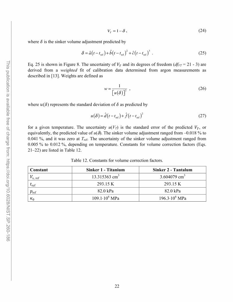
VT = 1−δ , (24)
where T is the sinker volume adjustment predicted by
δ = ˆ ) + ˆ )2 + ˆ )3 . (25)a t ( − tref b t ( − tref c t ( − tref
Eq. 25 is shown in Figure 8. The uncertainty of K0 and its degrees of freedom (dfVT = 21 - 3) are derived from a weighted fit of calibration data determined from argon measurements as described in [13]. Weights are defined as
1 w = , (26) u δ ⎤⎦
2⎡⎣ ( )
where *(T) represents the standard deviation of T as predicted by
u δ d t − tref ) + f tˆ ( − tref )2 (27)( ) = ˆ(
for a given temperature. The uncertainty u(VT) is the standard error of the predicted K0, or equivalently, the predicted value of u(δ). The sinker volume adjustment ranged from –0.018 % to 0.041 %, and it was zero at Tref. The uncertainty of the sinker volume adjustment ranged from 0.005 % to 0.012 %, depending on temperature. Constants for volume correction factors (Eqs. 21–22) are listed in Table 12.
Table 12. Constants for volume correction factors.
Constant Sinker 1 - Titanium Sinker 2 - Tantalum Kx, ref 13.315363 cm3 3.604079 cm3
Uref 293.15 K 293.15 K 2ref 82.0 kPa 82.0 kPa V7 109.1⋅106 MPa 196.3⋅106 MPa
22

______________________________________________________________________________________________________ This publication is available free of charge from
: https://doi.org/10.6028/NIS
T.SP
.260-186
Sink
er V
olum
e Ad
just
men
t (%
)
-0.03
-0.02
-0.01
0.00
0.01
0.02
0.03
0.04
0.05
-100 0 100 200 300 T - Tref (C)
Figure 8. Sinker volume adjustment (eq. 25) as a function of temperature. The reference temperature (Tref) is 20.00 ˚C, and the error bars represent standard uncertainties.
4.6.5.3 Sinker Volume, Lcal, Ltare
The cal and tare masses are housed in the balance chamber, i.e., at nearly constant temperature and pressure. Thus, the corrections needed for the density sinkers are not required. The type B uncertainty evaluations for sinker volume for the cal and tare sinkers are based on uniform distributions bounded by 0.05 % of the nominal sinker volume.
0.0005 ⋅Vcal 0.0005 ⋅Vtare ( ) = (28)and u Vtare u V( cal ) = 3 3
3 3Kcal = Ktare = 7.4788 cm , and the uncertainties are * Kcal = * Ktare = 0.002159 cm(dfVcal =dfVtare = 8).
4.6.6 Summary of u(ρfluid)
Uncertainty budgets for ρfluid, based on Eqs. 12–14, are shown in Tables 13 and 14 for two combinations of temperature and pressure. Table 15 gives the relative (percentage) contribution to the overall uncertainty in ρfluid from the different sources.
23

""
______________________________________________________________________________________________________ This publication is available free of charge from
: https://doi.org/10.6028/NIS
T.SP
.260-186
Table 13. Uncertainty budget for (fluid at 30 ˚C and 1 MPa. For this case,*((fluid) = 0.004 kg⋅m–3 and 8[eff = 21.
Source (J\) ]\ ]\ ∙ (J\)(kg⋅m –3)
Degrees of Freedom
+cal 2.10⋅10–6 g 33.1 6.94⋅10–5 11 +tare 1.66⋅10–6 g 44.47 7.38⋅10–5 11 Acal 6.74⋅10–6 g 33.1 2.23⋅10–4 11 Atare 6.75⋅10–6 g 44.47 3.00⋅10–4 10 Kcal 2.16⋅10–3 cm3 0.03 6.78⋅10–5 8 Ktare 2.16⋅10–3 cm3 0.04 9.11⋅10–5 8 (air 6.47⋅10–7 g/cm3 85.03 5.50⋅10–5 8 A: 8.13⋅10–6 g 98.73 8.02⋅10–4 8 A> 9.35⋅10–6 g 87.36 8.17⋅10–4 5 K: 4.76⋅10–5 cm3 67.6 3.22⋅10–3 10 K> 4.44⋅10–5 cm3 59.82 2.66⋅10–3 8 +: 2.08⋅10–6 g 98.72 2.05⋅10–4 11 +> 7.82⋅10–7 g 87.35 6.83⋅10–5 11 (7 3.47⋅10–8 g/cm3 1000 3.47⋅10–5 55
24

""
"
______________________________________________________________________________________________________ This publication is available free of charge from
: https://doi.org/10.6028/NIS
T.SP
.260-186
Table 14. Uncertainty budget for ρfluid at 160 ˚C and 30 MPa. For this case, u(ρfluid) = 0.012 kg⋅m–3 and dfeff = 10.
Source (J\) ]\ ]\ ∙ (J\)(kg⋅m –3)
Degrees of Freedom
+cal 1.73⋅10–6 g 30.15 5.22⋅10–5 11 +tare 1.87⋅10–6 g 40.51 7.57⋅10–5 11 Acal 6.74⋅10–6 g 30.16 2.03⋅10–4 11 Atare 6.75⋅10–6 g 40.51 2.73⋅10–4 10 Kcal 2.16⋅10–3 cm3 0.03 6.15⋅10–5 8 Ktare 2.16⋅10–3 cm3 0.04 8.26⋅10–5 8 (air 6.41⋅10–7 g/cm3 77.46 4.97⋅10–5 8 A: 8.13⋅10–6 g 98.76 8.03⋅10–4 8 A> 9.35⋅10–6 g 88.41 8.26⋅10–4 5 K: 1.87⋅10–4 cm3 61.62 1.15⋅10–2 9 K> 5.21⋅10–5 cm3 55.16 2.88⋅10–3 13 +: 1.74⋅10–6 g 98.76 1.72⋅10–4 11 +> 2.44⋅10–6 g 88.4 2.15⋅10–4 11 (7 3.06⋅10–8 g/cm3 1000 3.06⋅10–5 60
Table 15. Percentages of total variation in u(ρfluid) for six sources of uncertainty at various temperatures and pressures. The column labeled “all others” contains the combined percentage of total variation for the remaining eight sources. The value of u(ρfluid) is also listed. The quantities in the table represent average values for the given temperatures and pressures.
t (˚C)
p (MPa)
Percent of Total Variation
LM LN ^ cal ^ tare ^M ^N all
others (!fluid)
(kg⋅m–3) -5 1 55.2 37.1 0.3 0.5 3.2 3.2 0.5 0.005 -5 15 84.8 12.8 0.1 0.2 1 1 0.1 0.008 -5 30 93.7 5.5 0 0.1 0.3 0.3 0.1 0.014 30 1 54.6 37.3 0.3 0.5 3.4 3.5 0.4 0.004 30 30 93.5 5.6 0 0.1 0.4 0.4 0 0.014 160 1 52.0 36.7 0.2 0.4 4.7 5.1 0.8 0.004 160 15 82.2 14.3 0.1 0.2 1.5 1.6 0.1 0.007 160 30 93.1 5.8 0 0.1 0.5 0.5 0.1 0.012
25

______________________________________________________________________________________________________ This publication is available free of charge from
: https://doi.org/10.6028/NIS
T.SP
.260-186
5. Summary of Uncertainties
5.1 Combined Standard Uncertainty
Combined standard uncertainty, computed using Eq. 4 for degassed samples and excluding uncertainties due to the effects of the user’s temperature and pressure measurements, is listed in Table 16 for various combinations of temperature and pressure. (The value of u(Δ) is zero for degassed samples.)
When the SRM is used to calibrate a user’s densimeter, the uncertainties listed in Table 16 can be utilized in conjunction with uncertainties in the user’s temperature and pressure measurements, u(tp) (Table 4), and their level of fluid saturation, u(Δ).
5.2 Expanded Uncertainty and Degrees of Freedom
The average expanded uncertainty for degassed measurements reported in this document is 0.054 kg⋅m–3. The coverage factor, k, is approximately 2 based on a Student’s t distribution with 63 effective degrees of freedom. The effective degrees of freedom were computed using the Welch-Satterthwaite approximation. To obtain a conservative estimate of combined standard uncertainty, we used the largest value of u(e) (0.014 kg⋅m–3) and the smallest degrees of freedom associated with ρfluid (dfe = 10) across all temperatures and pressures.
26

______________________________________________________________________________________________________ This publication is available free of charge from
: https://doi.org/10.6028/NIS
T.SP
.260-186
Table 16. Combined standard uncertainty in ρc (kg⋅m–3) including the effects of*((), *(K), *(C), and *(_) for degassed samples.
t (˚C) Pressure (MPa)
0.1 1 2 5 10 15 20 25 30 -50 0.025 0.025 0.025 0.025 0.025 0.026 0.026 0.027 0.028 -40 0.025 0.025 0.025 0.025 0.025 0.026 0.026 0.027 0.028 -30 0.025 0.025 0.025 0.025 0.025 0.026 0.026 0.027 0.028 -20 0.025 0.025 0.025 0.025 0.025 0.026 0.026 0.027 0.028 -10 0.025 0.025 0.025 0.025 0.025 0.026 0.026 0.027 0.028 0 0.025 0.025 0.025 0.025 0.025 0.026 0.026 0.027 0.028 10 0.025 0.025 0.025 0.025 0.025 0.026 0.026 0.027 0.028 20 0.025 0.025 0.025 0.025 0.025 0.026 0.026 0.027 0.028 30 0.025 0.025 0.025 0.025 0.025 0.026 0.026 0.027 0.028 40 0.025 0.025 0.025 0.025 0.025 0.026 0.026 0.027 0.028 50 0.025 0.025 0.025 0.025 0.025 0.026 0.026 0.027 0.028 60 0.025 0.025 0.025 0.025 0.025 0.025 0.026 0.027 0.028 70 0.025 0.025 0.025 0.025 0.025 0.025 0.026 0.027 0.028 80 0.025 0.025 0.025 0.025 0.025 0.025 0.026 0.027 0.028 90 0.025 0.025 0.025 0.025 0.025 0.025 0.026 0.027 0.028 100 0.025 0.025 0.025 0.025 0.025 0.026 0.027 0.028 110 0.025 0.025 0.025 0.025 0.025 0.026 0.027 0.028 120 0.025 0.025 0.025 0.025 0.025 0.026 0.027 0.028 130 0.025 0.025 0.025 0.025 0.025 0.026 0.027 0.028 140 0.025 0.025 0.025 0.025 0.025 0.026 0.027 0.028 150 0.025 0.025 0.025 0.025 0.025 0.026 0.027 0.028 160 0.025 0.025 0.025 0.025 0.025 0.026 0.027 0.028
27

______________________________________________________________________________________________________ This publication is available free of charge from
: https://doi.org/10.6028/NIS
T.SP
.260-186
6. Discussion and Conclusions We report values for the density of liquid iso-octane that form the basis of NIST Standard Reference Material® 2214 “Iso-octane Liquid Density—Extended Range.” This work extends the range of this SRM, which was previously limited to 15 ˚C to 25 ˚C and normal atmospheric pressure, to the temperature range –50 ˚C to 160 ˚C and pressure range 0.1 MPa to 30 MPa. This SRM will be useful in the calibration of industrial densimeters.
The uncertainties for the density values were obtained by a thorough statistical analysis of multiple sources of uncertainty. In many cases, a measured quantity depended on other underlying measurands, and the uncertainties at each level were considered.
The measurements reported here are directly traceable to SI quantities. The density was determined by weighing sinkers immersed in the fluid. The volume (or, equivalently, density) of the sinkers was determined by comparison to solid density standards that are directly traceable to the meter and kilogram. The balance that carried out the weighings was calibrated for each density determination using calibration weights, which were, in turn, calibrated against standard masses. The temperature of the fluid was measured with a standard platinum resistance thermometer calibrated with ITS-90 fixed points. The pressure transducer was calibrated against a piston gage pressure standard.
28
______________________________________________________________________________________________________
This publication is available free of charge from: https://doi.org/10.6028/N
IST.S
P.260-186
References [1] McLinden, M. O., Lösch-Will, C. (2007) Apparatus for wide-ranging, high-accuracy fluid
(p, ρ, T) measurements based on a compact two-sinker densimeter. J. Chem. Thermodyn. 39, 507-530.
[2] McLinden, M., Splett, J. (2008) A Liquid Density Standard Over Wide Ranges of Temperature and Pressure Based on Toluene, J. Res. Nat. Inst. Stand. Techn., 113, 29-67.
[3] Wagner, W., Kleinrahm, R. (2004) Densimeters for very accurate density measurements of fluids over large ranges of temperature, pressure, and density. Metrologia, 41, S24-S39.
[4] McLinden, M. O., Kleinrahm, R., Wagner, W. (2007) Force transmission errors in magnetic suspension densimeters. Int. J. Thermophysics, 28, 429-448.
[5] Bean, V. E., Houser, J. F. (2000) Characterization of Iso-octane as a Liquid Density Standard, SRM 2214, Report of Analysis, April 6, 2000, National Institute of Standards and Technology.
[6] Span, R., Lemmon, E., Jacobsen, R., Wagner, W., Yokozeki, A. (2000) A reference equation of state for the thermodynamic properties of nitrogen for temperatures from 63.151 to 1000 K and pressures to 2200 MPa, J. Phys. Chem. Ref. Data, 29, 1361-1433.
[7] Harris, G. L., Torres, J. A. (2003) Selected laboratory and measurement practices and procedures, to support basic mass calibrations; NISTIR 6969; National Institute of Standards and Technology.
[8] Davis, R. S. (1992) Equation for the determination of the density of moist air (1981/91). Metrologia 29, 67-70.
[9] Lafarge, T., Possolo, A. (2015) NIST Uncertainty Machine - User’s Manual, http://stat.nist.gov/uncertainty/.
[10] International Organization for Standardization (1995) Guide to the Expression of Uncertainty in Measurement”, International Organization for Standardization, Geneva Switzerland (corrected and reprinted 1995).
[11] Bowman, H. A., Schoonover, R. M., Carroll, C. L. (1974) The utilization of solid objects as reference standards in density measurements, Metrologia, 10, 117-121.
[12] Touloukian, Y. S. (1975) Thermophysical Properties of Matter, 12, Thermal Expansion, Plenum, New York.
[13] McLinden, M. (2006) Densimetry for primary temperature metrology and a method for the in situ determination of densimeter sinker volumes,” Measurement Sci. Technology, 17, 2597-2612.
29
______________________________________________________________________________________________________ This publication is available free of charge from
: https://doi.org/10.6028/NIS
T.SP
.260-186
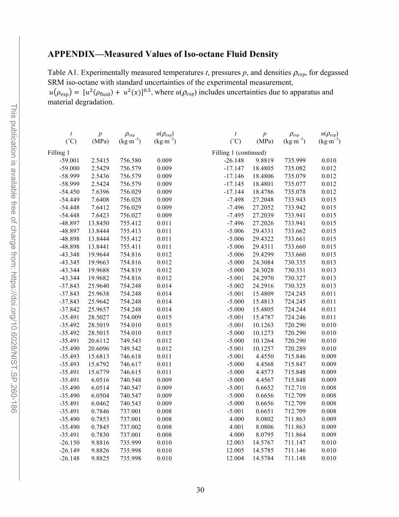
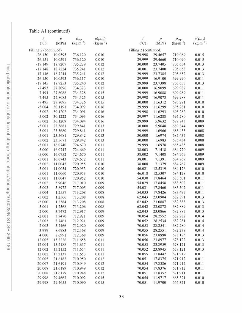
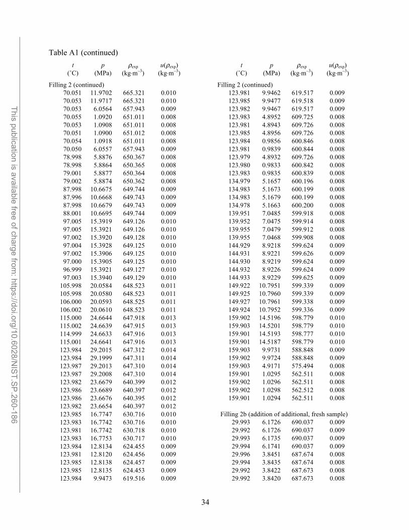
APPENDIX—Measured Values of Iso-octane Fluid Density
Table A1. Experimentally measured temperatures t, pressures p, and densities ρexp, for degassed SRM iso-octane with standard uncertainties of the experimental measurement,
>* (exp = * ( * (C) 7.h, where u(ρexp) includes uncertainties due to apparatus andfluid + >
material degradation.
t (˚C)
p (MPa)
ρexp (kg⋅m–3)
u(ρexp) (kg⋅m–3)
t (˚C)
p (MPa)
ρexp (kg⋅m–3)
u(ρexp) (kg⋅m–3)
Filling 1 Filling 1 (continued) -59.001 2.5415 756.580 0.009 -26.148 9.8819 735.999 0.010 -59.000 2.5429 756.579 0.009 -17.147 18.4805 735.082 0.012 -58.999 2.5436 756.579 0.009 -17.146 18.4806 735.079 0.012 -58.999 2.5424 756.579 0.009 -17.145 18.4801 735.077 0.012 -54.450 7.6396 756.029 0.009 -17.144 18.4786 735.078 0.012 -54.449 7.6408 756.028 0.009 -7.498 27.2048 733.943 0.015 -54.448 7.6412 756.029 0.009 -7.496 27.2052 733.942 0.015 -54.448 7.6423 756.027 0.009 -7.495 27.2039 733.941 0.015 -48.897 13.8450 755.412 0.011 -7.496 27.2026 733.941 0.015 -48.897 13.8444 755.413 0.011 -5.006 29.4331 733.662 0.015 -48.898 13.8444 755.412 0.011 -5.006 29.4322 733.661 0.015 -48.898 13.8441 755.411 0.011 -5.006 29.4311 733.660 0.015 -43.348 19.9644 754.816 0.012 -5.006 29.4299 733.660 0.015 -43.345 19.9663 754.816 0.012 -5.000 24.3084 730.335 0.013 -43.344 19.9688 754.819 0.012 -5.000 24.3028 730.331 0.013 -43.344 19.9682 754.816 0.012 -5.001 24.2970 730.327 0.013 -37.843 25.9640 754.248 0.014 -5.002 24.2916 730.325 0.013 -37.843 25.9638 754.248 0.014 -5.001 15.4809 724.245 0.011 -37.843 25.9642 754.248 0.014 -5.000 15.4813 724.245 0.011 -37.842 25.9657 754.248 0.014 -5.000 15.4805 724.244 0.011 -35.491 28.5027 754.009 0.015 -5.001 15.4787 724.246 0.011 -35.492 28.5019 754.010 0.015 -5.001 10.1263 720.290 0.010 -35.492 28.5015 754.010 0.015 -5.000 10.1273 720.290 0.010 -35.491 20.6112 749.543 0.012 -5.000 10.1264 720.290 0.010 -35.490 20.6096 749.542 0.012 -5.001 10.1257 720.289 0.010 -35.493 15.6813 746.618 0.011 -5.001 4.4550 715.846 0.009 -35.493 15.6792 746.617 0.011 -5.000 4.4568 715.847 0.009 -35.491 15.6779 746.615 0.011 -5.000 4.4573 715.848 0.009 -35.491 6.0516 740.548 0.009 -5.000 4.4567 715.848 0.009 -35.490 6.0514 740.547 0.009 -5.001 0.6652 712.710 0.008 -35.490 6.0504 740.547 0.009 -5.000 0.6656 712.709 0.008 -35.491 6.0462 740.543 0.009 -5.000 0.6656 712.709 0.008 -35.491 0.7846 737.001 0.008 -5.001 0.6651 712.709 0.008 -35.490 0.7853 737.001 0.008 4.000 8.0802 711.863 0.009 -35.490 0.7845 737.002 0.008 4.001 8.0806 711.863 0.009 -35.491 0.7830 737.001 0.008 4.000 8.0795 711.864 0.009 -26.150 9.8816 735.999 0.010 12.003 14.5767 711.147 0.010 -26.149 9.8826 735.998 0.010 12.005 14.5785 711.146 0.010 -26.148 9.8825 735.998 0.010 12.004 14.5784 711.148 0.010
30

______________________________________________________________________________________________________ This publication is available free of charge from
: https://doi.org/10.6028/NIS
T.SP
.260-186
Table A1 (continued) t
(˚C) p
(MPa) ρexp
(kg⋅m–3) u(ρexp)
(kg⋅m–3) t
(˚C) p
(MPa) ρexp
(kg⋅m–3) u(ρexp)
(kg⋅m–3)
Filling 1 (continued) Filling 1 (continued) 4.001 8.0807 711.863 0.009 70.002 20.1915 674.430 0.012
12.003 14.5779 711.147 0.010 70.001 27.4311 681.551 0.014 20.006 20.9783 710.455 0.012 69.998 20.1894 674.428 0.012 20.007 20.9796 710.455 0.012 70.002 20.1912 674.430 0.012 20.008 20.9797 710.454 0.012 69.998 15.9224 669.873 0.010 30.013 28.8184 709.596 0.015 70.001 15.9239 669.872 0.010 30.013 28.8184 709.595 0.015 70.001 15.9237 669.871 0.010 30.013 28.8190 709.595 0.015 69.998 15.9218 669.871 0.010 30.015 28.8197 709.595 0.015 70.001 10.6528 663.789 0.009 29.999 19.1125 701.869 0.012 69.999 10.6516 663.789 0.009 30.001 19.1126 701.867 0.012 69.997 10.6505 663.790 0.009 30.000 19.1116 701.866 0.012 69.999 10.6515 663.789 0.009 29.999 19.1106 701.867 0.012 70.001 5.2028 656.851 0.008 30.000 12.0436 695.664 0.010 69.998 5.2007 656.848 0.008 30.001 12.0447 695.664 0.010 69.998 5.2014 656.851 0.008 30.001 12.0444 695.664 0.010 70.000 5.2027 656.851 0.008 29.999 12.0430 695.664 0.010 70.001 1.2131 651.240 0.008 29.997 9.4033 693.200 0.009 69.998 1.2122 651.242 0.008 29.999 9.4042 693.200 0.009 70.001 1.2126 651.241 0.008 30.001 9.4054 693.199 0.009 70.001 1.2110 651.237 0.008 30.000 9.4039 693.199 0.009 78.996 6.0371 650.582 0.008 30.000 3.3476 687.178 0.008 78.998 6.0380 650.582 0.008 30.000 3.3471 687.178 0.008 79.000 6.0388 650.582 0.008 29.998 3.3461 687.177 0.008 78.998 6.0371 650.581 0.008 29.998 3.3461 687.178 0.008 87.998 10.8197 649.954 0.009 29.998 0.9986 684.688 0.008 87.997 10.8199 649.954 0.009 29.997 0.9982 684.689 0.008 87.999 10.8207 649.954 0.009 29.998 0.9996 684.689 0.008 88.002 10.8227 649.954 0.009 30.000 1.0003 684.688 0.008 97.006 15.5545 649.342 0.010 38.005 6.4264 684.026 0.009 97.008 15.5552 649.341 0.010 38.005 6.4258 684.026 0.009 97.005 15.5537 649.341 0.010 38.003 6.4256 684.026 0.009 97.008 15.5556 649.341 0.010 38.002 6.4251 684.027 0.009 106.004 20.2275 648.738 0.011 46.020 11.7886 683.380 0.010 106.007 20.2290 648.738 0.011 46.022 11.7902 683.380 0.010 106.006 20.2285 648.737 0.011 46.024 11.7908 683.379 0.010 115.001 24.8332 648.126 0.013 46.022 11.7898 683.380 0.010 115.005 24.8348 648.127 0.013 54.037 17.0838 682.752 0.011 115.004 24.8333 648.124 0.013 54.036 17.0831 682.751 0.011 115.000 24.8300 648.122 0.013 54.036 17.0837 682.752 0.011 124.994 29.8462 647.412 0.015 54.037 17.0847 682.752 0.011 124.995 29.8441 647.409 0.015 62.050 22.3140 682.145 0.012 124.998 29.8444 647.407 0.015 62.049 22.3133 682.144 0.012 124.998 29.8401 647.402 0.015 62.048 22.3131 682.145 0.012 124.997 21.4278 636.676 0.012 62.049 22.3136 682.145 0.012 124.995 21.4269 636.677 0.012 70.000 27.4320 681.552 0.014 124.997 17.5044 631.054 0.010 70.002 27.4307 681.550 0.014 124.995 17.4976 631.046 0.010 69.999 27.4293 681.550 0.014 124.993 17.4919 631.039 0.010 70.002 20.1926 674.431 0.012 124.996 14.3307 626.138 0.010
31

______________________________________________________________________________________________________ This publication is available free of charge from
: https://doi.org/10.6028/NIS
T.SP
.260-186
Table A1 (continued) t
(˚C) p
(MPa) ρexp
(kg⋅m–3) u(ρexp)
(kg⋅m–3) t
(˚C) p
(MPa) ρexp
(kg⋅m–3) u(ρexp)
(kg⋅m–3)
Filling 1 (continued) Filling 1b (continued) 124.993 14.3295 626.139 0.010 29.995 3.0531 686.858 0.008 124.994 14.3300 626.138 0.010 29.994 3.0531 686.857 0.008 124.997 17.4953 631.041 0.010 29.993 1.1100 684.795 0.008 124.997 14.3317 626.139 0.010 29.992 1.1077 684.794 0.008 134.979 18.7561 625.505 0.011 29.994 1.1084 684.793 0.008 134.983 18.7573 625.504 0.011 29.996 1.1087 684.790 0.008 134.983 18.7566 625.503 0.011 29.995 3.0530 686.857 0.008 134.979 18.7548 625.503 0.011 139.955 20.9461 625.198 0.011 Filling 2 139.958 20.9474 625.198 0.011 -58.996 1.6038 756.019 0.009 144.936 23.1192 624.880 0.012 -58.997 1.5999 756.019 0.009 144.936 23.1181 624.879 0.012 -58.998 1.5982 756.020 0.009 144.938 23.1190 624.878 0.012 -58.998 1.5973 756.018 0.009 144.941 23.1190 624.878 0.012 -58.999 1.5960 756.018 0.009 149.930 25.2859 624.565 0.013 -54.452 6.6806 755.472 0.009 149.929 25.2848 624.565 0.013 -54.451 6.6820 755.472 0.009 149.930 25.2855 624.565 0.013 -54.450 6.6836 755.471 0.009 149.933 25.2881 624.568 0.013 -54.449 6.6836 755.471 0.009 159.904 29.5738 623.938 0.014 -48.898 12.8810 754.860 0.010 159.903 29.5744 623.939 0.014 -43.346 18.9905 754.265 0.012 159.906 29.5765 623.940 0.014 -43.345 18.9917 754.265 0.012 159.907 29.5778 623.942 0.014 -43.345 18.9908 754.265 0.012 159.906 22.1354 612.635 0.012 -43.346 18.9900 754.266 0.012 159.907 22.1359 612.636 0.012 -37.845 24.9723 753.698 0.014 159.905 22.1354 612.636 0.012 -37.845 24.9722 753.698 0.014 159.904 22.1346 612.636 0.012 -37.844 24.9737 753.699 0.014 159.906 16.9606 603.539 0.010 -37.843 24.9746 753.696 0.014 159.905 16.9602 603.538 0.010 -35.493 27.5180 753.467 0.015 159.903 16.9603 603.540 0.010 -35.492 27.5170 753.466 0.015 159.903 16.9605 603.540 0.010 -35.491 27.5170 753.461 0.015 159.905 10.9573 591.135 0.009 -35.490 27.5171 753.462 0.015 159.907 10.9579 591.136 0.009 -35.491 20.7885 749.643 0.012 159.905 10.9576 591.136 0.009 -35.490 20.7881 749.647 0.012 159.903 10.9571 591.138 0.009 -35.490 20.7864 749.642 0.012 159.905 5.5680 577.397 0.008 -35.491 20.7858 749.645 0.012 159.905 5.5676 577.394 0.008 -35.493 17.2838 747.581 0.011 159.903 5.5668 577.393 0.008 -35.493 17.2837 747.582 0.011 159.901 5.5663 577.394 0.008 -35.492 17.2853 747.577 0.011 159.905 1.4130 563.945 0.008 -35.490 17.2882 747.584 0.011 159.906 1.4119 563.938 0.008 -35.491 10.3697 743.330 0.010 159.904 1.4108 563.938 0.008 -35.490 10.3714 743.326 0.010 159.902 1.4098 563.934 0.008 -35.489 10.3720 743.334 0.010
-35.490 10.3712 743.331 0.010 Filling 1b (addition of additional, fresh sample)
29.992 6.9293 690.791 0.009 -35.492 -35.490
5.5763 5.5778
740.236 740.234
0.009 0.009
29.992 6.9295 690.792 0.009 -35.490 5.5786 740.235 0.009 29.992 6.9298 690.793 0.009 -35.491 5.5782 740.236 0.009 29.993 6.9312 690.792 0.009 -35.492 0.9248 737.098 0.008 29.994 3.0523 686.845 0.008 -26.151 10.0586 736.117 0.010
32
______________________________________________________________________________________________________ This publication is available free of charge from
: https://doi.org/10.6028/NIS
T.SP
.260-186
Table A1 (continued) t
(˚C) p
(MPa) ρexp
(kg⋅m–3) u(ρexp)
(kg⋅m–3) t
(˚C) p
(MPa) ρexp
(kg⋅m–3) u(ρexp)
(kg⋅m–3)
Filling 2 (continued) Filling 2 (continued) -26.150 10.0595 736.120 0.010 29.998 29.4657 710.089 0.015 -26.151 10.0591 736.120 0.010 29.999 29.4660 710.090 0.015 -17.149 18.7207 735.239 0.012 30.000 23.7405 705.654 0.013 -17.148 18.7224 735.241 0.012 30.001 23.7400 705.653 0.013 -17.146 18.7244 735.241 0.012 29.999 23.7385 705.652 0.013 -26.150 10.0593 736.117 0.010 29.999 16.9100 699.990 0.011 -17.145 18.7253 735.240 0.012 29.999 23.7398 705.655 0.013
-7.493 27.8096 734.323 0.015 30.000 16.9099 699.987 0.011 -7.494 27.8088 734.328 0.015 29.999 16.9088 699.989 0.011 -7.495 27.8085 734.325 0.015 29.998 16.9073 699.988 0.011 -7.495 27.8095 734.326 0.015 30.000 11.6312 695.281 0.010 -5.004 30.1191 734.092 0.016 29.999 11.6299 695.281 0.010 -5.002 30.1202 734.091 0.016 29.998 11.6293 695.282 0.010 -5.002 30.1222 734.093 0.016 29.997 11.6288 695.280 0.010 -5.002 30.1209 734.094 0.016 29.999 5.9632 689.843 0.009 -5.001 23.5681 729.841 0.013 30.000 5.9648 689.844 0.009 -5.001 23.5680 729.841 0.013 29.999 1.6966 685.435 0.008 -5.001 23.5681 729.842 0.013 30.000 1.6974 685.435 0.008 -5.002 23.5671 729.842 0.013 30.000 1.6983 685.434 0.008 -5.001 16.0740 724.670 0.011 29.999 1.6978 685.435 0.008 -5.000 16.0747 724.669 0.011 38.003 7.1418 684.770 0.009 -5.000 16.0752 724.670 0.011 38.002 7.1408 684.769 0.009 -5.001 16.0743 724.672 0.011 38.001 7.1391 684.769 0.009 -5.002 11.0045 720.955 0.010 38.000 7.1379 684.767 0.009 -5.001 11.0054 720.953 0.010 46.021 12.5319 684.126 0.010 -5.001 11.0060 720.953 0.010 46.018 12.5307 684.128 0.010 -5.001 11.0047 720.952 0.010 54.030 17.8464 683.501 0.011 -5.002 5.9046 717.010 0.009 54.029 17.8458 683.502 0.011 -5.003 5.8972 717.005 0.009 54.031 17.8460 683.502 0.011 -5.004 1.2557 713.208 0.008 54.033 17.8426 683.497 0.011 -5.002 1.2566 713.208 0.008 62.043 23.0904 682.891 0.013 -5.000 1.2584 713.208 0.008 62.042 23.0887 682.888 0.013 -5.001 1.2568 713.206 0.008 62.042 23.0872 682.889 0.013 -2.000 3.7472 712.917 0.009 62.043 23.0866 682.887 0.013 -2.001 3.7470 712.921 0.009 70.054 28.2552 682.282 0.014 -2.003 3.7461 712.921 0.009 70.052 28.2534 682.281 0.014 -2.003 3.7466 712.920 0.009 70.053 28.2541 682.280 0.014 3.999 8.6983 712.368 0.009 70.055 28.2551 682.279 0.014 4.000 8.6991 712.368 0.009 70.056 23.8998 678.125 0.013
12.005 15.2226 711.658 0.011 70.056 23.8977 678.122 0.013 12.004 15.2188 711.657 0.011 70.053 23.8959 678.121 0.013 12.002 15.2152 711.654 0.011 70.052 23.8945 678.121 0.013 12.002 15.2137 711.653 0.011 70.055 17.8442 671.919 0.011 20.005 21.6182 710.950 0.012 70.051 17.8375 671.912 0.011 20.007 21.6191 710.949 0.012 70.054 17.8386 671.912 0.011 20.008 21.6189 710.949 0.012 70.054 17.8376 671.912 0.011 20.008 21.6179 710.948 0.012 70.051 17.8352 671.911 0.011 29.998 29.4663 710.092 0.015 70.054 11.9717 665.321 0.010 29.998 29.4655 710.090 0.015 70.051 11.9700 665.321 0.010
33
______________________________________________________________________________________________________ This publication is available free of charge from
: https://doi.org/10.6028/NIS
T.SP
.260-186
Table A1 (continued) t
(˚C) p
(MPa) ρexp
(kg⋅m–3) u(ρexp)
(kg⋅m–3) t
(˚C) p
(MPa) ρexp
(kg⋅m–3) u(ρexp)
(kg⋅m–3)
Filling 2 (continued) Filling 2 (continued) 70.051 11.9702 665.321 0.010 123.981 9.9462 619.517 0.009 70.053 11.9717 665.321 0.010 123.985 9.9477 619.518 0.009 70.053 6.0564 657.943 0.009 123.982 9.9467 619.517 0.009 70.055 1.0920 651.011 0.008 123.983 4.8952 609.725 0.008 70.053 1.0908 651.011 0.008 123.981 4.8943 609.726 0.008 70.051 1.0900 651.012 0.008 123.985 4.8956 609.726 0.008 70.054 1.0918 651.011 0.008 123.984 0.9856 600.846 0.008 70.050 6.0557 657.943 0.009 123.981 0.9839 600.844 0.008 78.998 5.8876 650.367 0.008 123.979 4.8932 609.726 0.008 78.998 5.8864 650.365 0.008 123.980 0.9833 600.842 0.008 79.001 5.8877 650.364 0.008 123.983 0.9835 600.839 0.008 79.002 5.8874 650.362 0.008 134.979 5.1657 600.196 0.008 87.998 10.6675 649.744 0.009 134.983 5.1673 600.199 0.008 87.996 10.6668 649.743 0.009 134.983 5.1679 600.199 0.008 87.998 10.6679 649.743 0.009 134.978 5.1663 600.200 0.008 88.001 10.6695 649.744 0.009 139.951 7.0485 599.918 0.008 97.005 15.3919 649.126 0.010 139.952 7.0475 599.914 0.008 97.005 15.3921 649.126 0.010 139.955 7.0479 599.912 0.008 97.002 15.3920 649.128 0.010 139.955 7.0468 599.908 0.008 97.004 15.3928 649.125 0.010 144.929 8.9218 599.624 0.009 97.002 15.3906 649.125 0.010 144.931 8.9221 599.626 0.009 97.000 15.3905 649.125 0.010 144.930 8.9219 599.624 0.009 96.999 15.3921 649.127 0.010 144.932 8.9226 599.624 0.009 97.003 15.3940 649.129 0.010 144.933 8.9229 599.625 0.009
105.998 20.0584 648.523 0.011 149.922 10.7951 599.339 0.009 105.998 20.0580 648.523 0.011 149.925 10.7960 599.339 0.009 106.000 20.0593 648.525 0.011 149.927 10.7961 599.338 0.009 106.002 20.0610 648.523 0.011 149.924 10.7952 599.336 0.009 115.000 24.6644 647.918 0.013 159.902 14.5196 598.779 0.010 115.002 24.6639 647.915 0.013 159.903 14.5201 598.779 0.010 114.999 24.6633 647.916 0.013 159.901 14.5193 598.777 0.010 115.001 24.6641 647.916 0.013 159.901 14.5187 598.779 0.010 123.984 29.2015 647.312 0.014 159.903 9.9731 588.848 0.009 123.984 29.1999 647.311 0.014 159.902 9.9724 588.848 0.009 123.987 29.2013 647.310 0.014 159.903 4.9171 575.494 0.008 123.987 29.2008 647.310 0.014 159.901 1.0295 562.511 0.008 123.982 23.6679 640.399 0.012 159.902 1.0296 562.511 0.008 123.986 23.6689 640.397 0.012 159.902 1.0298 562.512 0.008 123.986 23.6676 640.395 0.012 159.901 1.0294 562.511 0.008 123.982 23.6654 640.397 0.012 123.985 16.7747 630.716 0.010 Filling 2b (addition of additional, fresh sample) 123.983 16.7742 630.716 0.010 29.993 6.1726 690.037 0.009 123.981 16.7742 630.718 0.010 29.992 6.1726 690.037 0.009 123.983 16.7753 630.717 0.010 29.993 6.1735 690.037 0.009 123.984 12.8134 624.455 0.009 29.994 6.1741 690.037 0.009 123.981 12.8120 624.456 0.009 29.996 3.8451 687.674 0.008 123.985 12.8138 624.457 0.009 29.994 3.8435 687.674 0.008 123.985 12.8135 624.453 0.009 29.992 3.8422 687.673 0.008 123.984 9.9473 619.516 0.009 29.992 3.8420 687.673 0.008
34

______________________________________________________________________________________________________ This publication is available free of charge from
: https://doi.org/10.6028/NIS
T.SP
.260-186
Table A1 (continued) t
(˚C) p
(MPa) ρexp
(kg⋅m–3) u(ρexp)
(kg⋅m–3) t
(˚C) p
(MPa) ρexp
(kg⋅m–3) u(ρexp)
(kg⋅m–3)
Filling 2b (continued) Filling 3 (continued) 29.993 1.1283 684.809 0.008 -5.003 18.1353 726.126 0.011 29.992 1.1281 684.809 0.008 -5.002 5.5103 716.691 0.009 29.993 1.1286 684.810 0.008 -5.002 5.5107 716.694 0.009 29.994 1.1300 684.810 0.008 -5.003 5.5092 716.689 0.009 62.017 22.4431 682.276 0.012 -5.004 5.5088 716.693 0.009 62.018 22.4439 682.276 0.012 -5.003 1.2422 713.193 0.008 62.020 22.4447 682.275 0.012 -5.002 1.2441 713.195 0.008 62.020 22.4438 682.273 0.012 -5.002 1.2445 713.195 0.008
-5.003 1.2441 713.195 0.008 Filling 3 29.998 29.4661 710.089 0.015
-58.996 1.9346 756.216 0.009 29.999 29.4674 710.088 0.015 -58.997 1.9321 756.214 0.009 30.000 29.4665 710.088 0.015 -58.998 1.9275 756.211 0.009 30.000 29.4676 710.089 0.015 -58.998 1.9267 756.211 0.009 29.997 22.4838 704.644 0.013 -48.899 13.2465 755.068 0.010 30.000 22.4847 704.645 0.013 -48.899 13.2488 755.069 0.010 29.998 22.4830 704.645 0.013 -48.897 13.2505 755.068 0.010 29.997 22.4814 704.643 0.013 -35.493 27.8960 753.672 0.015 29.998 17.0552 700.113 0.011 -35.492 27.8972 753.672 0.015 29.999 17.0560 700.114 0.011 -35.493 27.8981 753.674 0.015 29.998 17.0550 700.115 0.011 -35.492 8.1206 741.890 0.009 29.997 17.0552 700.114 0.011 -35.491 8.1206 741.891 0.009 29.997 5.5912 689.472 0.009 -35.493 1.6483 737.596 0.008 29.999 5.5930 689.470 0.009 -35.492 1.6481 737.591 0.008 29.999 5.5936 689.471 0.009 -35.492 1.6500 737.592 0.008 29.998 5.5930 689.470 0.009 -35.492 1.6506 737.591 0.008 29.998 0.8371 684.510 0.008
-5.007 29.7592 733.864 0.016 30.000 0.8375 684.510 0.008 -5.005 29.7613 733.864 0.016 29.999 0.8368 684.508 0.008 -5.005 29.7616 733.864 0.016 62.036 22.1299 681.975 0.012 -5.006 29.7623 733.864 0.016 62.033 22.1288 681.974 0.012 -5.004 18.1349 726.127 0.011 62.031 22.1281 681.976 0.012 -5.002 18.1368 726.125 0.011 62.033 22.1290 681.975 0.012 -5.002 18.1363 726.127 0.011
35
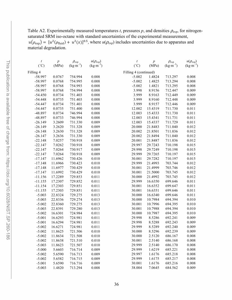
______________________________________________________________________________________________________ This publication is available free of charge from
: https://doi.org/10.6028/NIS
T.SP
.260-186
Table A2. Experimentally measured temperatures t, pressures p, and densities ρexp, for nitrogen-saturated SRM iso-octane with standard uncertainties of the experimental measurement,
>* (exp = * ( * (C) 7.h, where u(ρexp) includes uncertainties due to apparatus andfluid + >
material degradation.
t (˚C)
p (MPa)
ρexp (kg⋅m–3)
u(ρexp) (kg⋅m–3)
t (˚C)
p (MPa)
ρexp (kg⋅m–3)
u(ρexp) (kg⋅m–3)
Filling 4 Filling 4 (continued) -58.997 0.0767 754.994 0.008 -5.002 1.4824 713.297 0.008 -58.997 0.0768 754.995 0.008 -5.002 1.4825 713.294 0.008 -58.997 0.0768 754.993 0.008 -5.002 1.4821 713.295 0.008 -58.997 0.0768 754.994 0.008 3.998 8.9156 712.447 0.009 -54.450 0.0734 751.403 0.008 3.999 8.9163 712.449 0.009 -54.448 0.0735 751.403 0.008 3.999 8.9160 712.448 0.009 -54.447 0.0734 751.401 0.008 3.999 8.9157 712.446 0.009 -54.447 0.0735 751.400 0.008 12.002 15.4319 711.730 0.011 -48.897 0.0734 746.994 0.008 12.003 15.4333 711.730 0.011 -48.897 0.0733 746.994 0.008 12.003 15.4341 711.731 0.011 -26.149 3.2609 731.330 0.009 12.003 15.4337 711.729 0.011 -26.149 3.2620 731.328 0.009 20.000 21.8483 711.040 0.012 -26.148 3.2630 731.328 0.009 20.002 21.8501 711.036 0.012 -26.147 3.2636 731.330 0.009 20.002 21.8494 711.040 0.012 -22.148 7.0257 730.918 0.009 20.001 21.8487 711.036 0.012 -22.147 7.0262 730.918 0.009 29.997 29.7243 710.198 0.015 -22.147 7.0264 730.917 0.009 29.998 29.7249 710.198 0.015 -22.147 7.0264 730.918 0.009 29.999 29.7265 710.197 0.015 -17.147 11.6962 730.426 0.010 30.001 29.7282 710.197 0.015 -17.148 11.6966 730.423 0.010 29.999 21.4993 703.744 0.012 -17.148 11.6977 730.429 0.010 30.001 21.4999 703.746 0.012 -17.147 11.6992 730.429 0.010 30.001 21.5000 703.745 0.012 -11.156 17.2289 729.853 0.011 30.000 21.4992 703.745 0.012 -11.155 17.2307 729.852 0.011 29.999 16.6350 699.646 0.011 -11.154 17.2303 729.851 0.011 30.001 16.6352 699.647 0.011 -11.155 17.2303 729.851 0.011 30.001 16.6351 699.646 0.011
-5.003 22.8324 729.275 0.013 30.000 16.6340 699.646 0.011 -5.003 22.8336 729.274 0.013 30.000 10.7984 694.394 0.010 -5.002 22.8360 729.275 0.013 30.001 10.7996 694.395 0.010 -5.003 22.8391 729.280 0.013 30.001 10.7988 694.394 0.010 -5.002 16.6301 724.984 0.011 30.000 10.7987 694.395 0.010 -5.001 16.6293 724.981 0.011 29.998 8.5286 692.241 0.009 -5.001 16.6294 724.981 0.011 29.998 8.5288 692.243 0.009 -5.002 16.6271 724.981 0.011 29.999 8.5289 692.240 0.009 -5.002 11.8625 721.506 0.010 30.000 8.5296 692.239 0.009 -5.002 11.8634 721.508 0.010 30.000 2.5120 686.167 0.008 -5.002 11.8638 721.510 0.010 30.001 2.5140 686.168 0.008 -5.003 11.8623 721.507 0.010 29.999 2.5140 686.170 0.008 -5.000 5.6603 716.714 0.009 29.999 1.6219 685.221 0.008 -5.002 5.6590 716.713 0.009 29.997 1.6176 685.218 0.008 -5.002 5.6582 716.715 0.009 29.999 1.6175 685.217 0.008 -5.001 5.6590 716.716 0.009 30.001 1.6176 685.216 0.008 -5.003 1.4820 713.294 0.008 38.004 7.0645 684.562 0.009
36

______________________________________________________________________________________________________ This publication is available free of charge from
: https://doi.org/10.6028/NIS
T.SP
.260-186
Table A2 (continued) t
(˚C) p
(MPa) ρexp
(kg⋅m–3) u(ρexp)
(kg⋅m–3) t
(˚C) p
(MPa) ρexp
(kg⋅m–3) u(ρexp)
(kg⋅m–3)
Filling 4 (continued) Filling 4 (continued) 38.005 7.0634 684.559 0.009 97.003 15.7114 649.388 0.010 38.004 7.0590 684.555 0.009 106.007 20.3773 648.769 0.011 38.002 7.0556 684.551 0.009 106.004 20.3740 648.767 0.011 46.001 12.4222 683.908 0.010 106.008 20.3760 648.768 0.011 45.999 12.4172 683.904 0.010 106.008 20.3755 648.767 0.011 46.001 12.4154 683.902 0.010 114.995 24.9765 648.159 0.013 46.004 12.4162 683.900 0.010 114.991 24.9789 648.164 0.013 54.004 17.7096 683.268 0.011 114.995 24.9810 648.162 0.013 54.003 17.7079 683.268 0.011 114.994 24.9806 648.164 0.013 54.003 17.7069 683.267 0.011 124.978 30.0198 647.484 0.015 54.004 17.7069 683.267 0.011 124.981 30.0202 647.483 0.015 61.996 22.9366 682.661 0.012 124.982 30.0158 647.476 0.015 61.998 22.9387 682.660 0.012 124.979 30.0125 647.474 0.015 62.000 22.9397 682.661 0.012 124.982 24.5355 640.683 0.013 61.996 22.9379 682.662 0.012 124.981 24.5351 640.679 0.013 70.001 28.0849 682.047 0.014 124.980 19.2825 633.498 0.011 70.000 28.0830 682.045 0.014 124.980 19.2812 633.496 0.011 70.001 28.0825 682.045 0.014 124.978 19.2798 633.496 0.011 70.002 28.0826 682.044 0.014 124.976 19.2785 633.494 0.011 70.004 22.6867 676.838 0.012 124.980 10.4804 619.437 0.009 70.001 22.6854 676.844 0.012 124.978 10.4801 619.437 0.009 70.000 22.6884 676.840 0.012 124.976 10.4800 619.438 0.009 70.003 22.6905 676.843 0.012 124.980 10.4814 619.437 0.009 70.003 18.0811 672.078 0.011 135.001 14.7590 618.821 0.010 70.000 18.0779 672.078 0.011 135.001 14.7582 618.819 0.010 69.999 18.0735 672.073 0.011 134.998 14.7569 618.819 0.010 70.002 18.0745 672.070 0.011 134.997 14.7566 618.821 0.010 70.003 11.6303 664.811 0.009 139.988 16.8712 618.520 0.010 70.003 11.6312 664.810 0.009 139.986 16.8687 618.514 0.010 70.000 11.6297 664.812 0.009 139.987 16.8679 618.513 0.010 70.002 6.1395 657.933 0.009 139.988 16.8672 618.511 0.010 70.003 6.1380 657.929 0.009 144.991 18.9718 618.201 0.011 70.001 6.1363 657.929 0.009 144.990 18.9702 618.200 0.011 69.998 6.1347 657.928 0.009 144.992 18.9707 618.202 0.011 70.001 1.3811 651.305 0.008 144.994 18.9706 618.199 0.011 70.002 1.3798 651.302 0.008 149.997 21.0656 617.894 0.011 69.998 1.3763 651.300 0.008 149.997 21.0639 617.893 0.011 70.001 1.3780 651.299 0.008 149.998 21.0638 617.892 0.011 79.003 6.2097 650.644 0.009 149.999 21.0627 617.890 0.011 79.003 6.2099 650.645 0.009 159.996 25.2179 617.289 0.013 79.006 6.2113 650.647 0.009 159.994 25.2180 617.293 0.013 79.006 6.2112 650.645 0.009 159.995 25.2183 617.292 0.013 88.004 10.9881 650.010 0.009 159.998 23.7821 615.043 0.012 88.007 10.9906 650.011 0.009 159.997 23.7815 615.044 0.012 88.007 10.9911 650.011 0.009 159.997 23.7812 615.043 0.012 88.003 10.9900 650.014 0.009 159.997 23.7800 615.042 0.012 97.002 15.7108 649.387 0.010 159.997 17.9722 605.132 0.010 97.005 15.7121 649.388 0.010 159.996 17.9712 605.132 0.010 97.006 15.7130 649.387 0.010 159.994 17.9702 605.130 0.010
37

______________________________________________________________________________________________________ This publication is available free of charge from
: https://doi.org/10.6028/NIS
T.SP
.260-186
Table A2 (continued) t
(˚C) p
(MPa) ρexp
(kg⋅m–3) u(ρexp)
(kg⋅m–3)
Filling 4 (continued) 159.994 17.9697 605.131 0.010 159.998 12.0608 593.278 0.009 159.996 12.0604 593.278 0.009 159.994 12.0599 593.277 0.009 159.994 12.0599 593.280 0.009 159.995 6.0465 578.362 0.008 159.997 6.0468 578.362 0.008 159.995 6.0460 578.361 0.008 159.994 6.0457 578.362 0.008 159.996 1.4547 563.615 0.008 159.997 1.4542 563.611 0.008 159.995 1.4534 563.610 0.008 159.994 1.4524 563.607 0.008
38