Certifying Algorithms

R. M. McConnella, K. Mehlhornb,∗, S. Naherc, P. Schweitzerd

aComputer Science Department, Colorado State University Fort Collins, USAbMax Planck Institute for Informatics and Saarland University, Saarbrucken, Germany

cFachbereich Informatik, Universitat Trier, Trier, GermanydMax Planck Institute for Informatics, Saarbrucken, Germany

Abstract

A certifying algorithm is an algorithm that produces, with each output, a certificate or witness(easy-to-verify proof) that the particular output has not been compromised by a bug. A user of acertifying algorithm inputsx, receives the outputy and the certificatew, and then checks, eithermanually or by use of a program, thatw proves thaty is a correct output for inputx. In this way,he/she can be sure of the correctness of the output without having to trust the algorithm.

We put forward the thesis that certifying algorithms are much superior to non-certifying al-gorithms, and that for complex algorithmic tasks, only certifying algorithms are satisfactory.Acceptance of this thesis would lead to a change of how algorithms are taught and how algo-rithms are researched. The widespread use of certifying algorithms would greatly enhance thereliability of algorithmic software.

We survey the state of the art in certifying algorithms and add to it. In particular, we start atheory of certifying algorithms and prove that the concept is universal.

Contents

1 Introduction 4

2 First Examples 82.1 Tutorial Example 1: Testing Whether a Graph is Bipartite. . . . . . . . . . . . . 82.2 Tutorial Example 2: The Connected Components of an Undirected Graph . . . . 92.3 Tutorial Example 3: Greatest Common Divisor. . . . . . . . . . . . . . . . . . 92.4 Tutorial Example 4: Shortest Path Trees. . . . . . . . . . . . . . . . . . . . . . 112.5 Example: Maximum Cardinality Matchings in Graphs. . . . . . . . . . . . . . . 122.6 Case Study: The LEDA Planar Embedding Package. . . . . . . . . . . . . . . . 13

3 Examples of Program Failures 18

4 Relation to Extant Work 19

∗Corresponding Author

Preprint submitted to Elsevier August 30, 2010

5 Definitions and Formal Framework 215.1 Strongly Certifying Algorithms. . . . . . . . . . . . . . . . . . . . . . . . . . . 225.2 Certifying Algorithms. . . . . . . . . . . . . . . . . . . . . . . . . . . . . . . . 235.3 Weakly Certifying Algorithms . . . . . . . . . . . . . . . . . . . . . . . . . . . 245.4 Efficiency . . . . . . . . . . . . . . . . . . . . . . . . . . . . . . . . . . . . . . 255.5 Simplicity and Checkability . . . . . . . . . . . . . . . . . . . . . . . . . . . . 275.6 Deterministic Programs with Trivial Preconditions. . . . . . . . . . . . . . . . 295.7 Non-Trivial Preconditions . . . . . . . . . . . . . . . . . . . . . . . . . . . . . 305.8 An Objection . . . . . . . . . . . . . . . . . . . . . . . . . . . . . . . . . . . . 32

6 Checkers 326.1 The Pragmatic Approach. . . . . . . . . . . . . . . . . . . . . . . . . . . . . . 336.2 Manipulation of the Input. . . . . . . . . . . . . . . . . . . . . . . . . . . . . . 336.3 Formal Verification of Checkers. . . . . . . . . . . . . . . . . . . . . . . . . . 34

7 Advantages of Certifying Algorithms 34

8 General Techniques 368.1 Reduction. . . . . . . . . . . . . . . . . . . . . . . . . . . . . . . . . . . . . . 36

8.1.1 An Example . . . . . . . . . . . . . . . . . . . . . . . . . . . . . . . . 378.1.2 The General Approach. . . . . . . . . . . . . . . . . . . . . . . . . . . 40

8.2 Linear Programming Duality. . . . . . . . . . . . . . . . . . . . . . . . . . . . 418.3 Characterization Theorems. . . . . . . . . . . . . . . . . . . . . . . . . . . . . 478.4 Approximation Algorithms and Problem Relaxation. . . . . . . . . . . . . . . . 478.5 Composition of Programs. . . . . . . . . . . . . . . . . . . . . . . . . . . . . . 51

9 Further Examples 519.1 Convexity of Higher-dimensional Polyhedra and Convex Hulls . . . . . . . . . . 519.2 Solving Linear Systems of Equations. . . . . . . . . . . . . . . . . . . . . . . . 559.3 NP-Complete Problems. . . . . . . . . . . . . . . . . . . . . . . . . . . . . . . 569.4 Maximum Weight Independent Sets in Interval Graphs. . . . . . . . . . . . . . 579.5 String Matching. . . . . . . . . . . . . . . . . . . . . . . . . . . . . . . . . . . 599.6 Chordal Graphs. . . . . . . . . . . . . . . . . . . . . . . . . . . . . . . . . . . 609.7 Numerical Algorithms . . . . . . . . . . . . . . . . . . . . . . . . . . . . . . . 629.8 Guide to Literature. . . . . . . . . . . . . . . . . . . . . . . . . . . . . . . . . 63

10 Randomization 6410.1 Monte Carlo Algorithms resist Deterministic Certification . . . . . . . . . . . . . 6410.2 Integer Arithmetic. . . . . . . . . . . . . . . . . . . . . . . . . . . . . . . . . . 6510.3 Matrix Operations. . . . . . . . . . . . . . . . . . . . . . . . . . . . . . . . . . 6710.4 Cycle Bases. . . . . . . . . . . . . . . . . . . . . . . . . . . . . . . . . . . . . 6810.5 Definitions. . . . . . . . . . . . . . . . . . . . . . . . . . . . . . . . . . . . . . 72

11 Certification and Verification 75

2

12 Reactive Programs and Data Structures 7612.1 The Dictionary Problem. . . . . . . . . . . . . . . . . . . . . . . . . . . . . . 7712.2 Priority Queues. . . . . . . . . . . . . . . . . . . . . . . . . . . . . . . . . . . 79

13 Teaching Algorithms 84

14 Future Work 85

15 Conclusions 85

16 Acknowledgements 85

3

Program forfx y

Certifyingprogram forf

CheckerCx

x y

w

accepty

reject

Figure 1: The top figure shows the I/O behavior of a conventional program for computing a functionf . The userfeeds an inputx to the program and the program returns an outputy. The user of the program has no way of knowingwhethery is equal tof (x).The bottom figure shows the I/O behavior of a certifying algorithm, which computesy and a witnessw. The checkerC accepts the triple(x,y,w) if and only if w is a valid witness for the equalityy = f (x).

1. Introduction

One of the most prominent and costly problems in software engineering is correctness ofsoftware. When the user givesx as an input and the program outputsy, the user usually has noway of knowing whethery is a correct output on inputx or whether it has been compromised by abug. The user is at the mercy of the program. Acertifying algorithmis an algorithm that produceswith each output acertificateor witnessthat theparticular outputhas not been compromised bya bug. By inspecting the witness, the user can convince himself that the output is correct, orreject the output as buggy. He is no longer on the mercy of the program. Figure1 contrasts astandard algorithm with a certifying algorithm for computing a functionf .

A user of a certifying algorithm inputsx and receives the outputy and the witnessw. Hethen checks thatw proves thaty is a correct output for inputx. The process of checkingw canbe automated with achecker, which is an algorithm for verifying thatw proves thaty is a correctoutput forx. In may cases, the checker is so simple that a trusted implementation of it can beproduced, perhaps even in a different language where the semantics are fully specified. A formalproof of correctness of the implementation of the certifying algorithm may be out of reach,however, a formal proof of the correctness of the checker maybe feasible. Having checked thewitness, the user may proceed with complete confidence that outputy has not been compromised.

We want to stress that it does not suffice for the checker to be asimple algorithm. It is equallyimportant that it also easy for a user to understandwhy wproves thaty is a correct output forinputx.

4

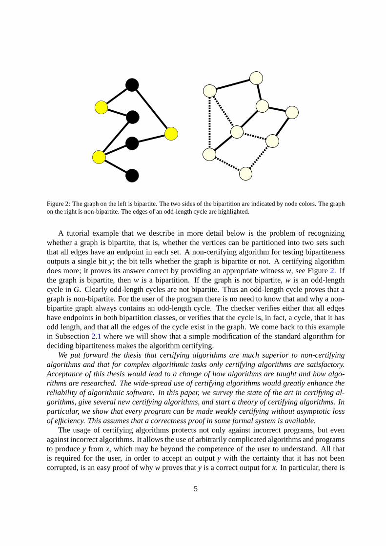
Figure 2: The graph on the left is bipartite. The two sides of the bipartition are indicated by node colors. The graphon the right is non-bipartite. The edges of an odd-length cycle are highlighted.

A tutorial example that we describe in more detail below is the problem of recognizingwhether a graph is bipartite, that is, whether the vertices can be partitioned into two sets suchthat all edges have an endpoint in each set. A non-certifyingalgorithm for testing bipartitenessoutputs a single bity; the bit tells whether the graph is bipartite or not. A certifying algorithmdoes more; it proves its answer correct by providing an appropriate witnessw, see Figure2. Ifthe graph is bipartite, thenw is a bipartition. If the graph is not bipartite,w is an odd-lengthcycle inG. Clearly odd-length cycles are not bipartite. Thus an odd-length cycle proves that agraph is non-bipartite. For the user of the program there is no need to know that and why a non-bipartite graph always contains an odd-length cycle. The checker verifies either that all edgeshave endpoints in both bipartition classes, or verifies thatthe cycle is, in fact, a cycle, that it hasodd length, and that all the edges of the cycle exist in the graph. We come back to this examplein Subsection2.1 where we will show that a simple modification of the standard algorithm fordeciding bipartiteness makes the algorithm certifying.

We put forward the thesis that certifying algorithms are much superior to non-certifyingalgorithms and that for complex algorithmic tasks only certifying algorithms are satisfactory.Acceptance of this thesis would lead to a change of how algorithms are taught and how algo-rithms are researched. The wide-spread use of certifying algorithms would greatly enhance thereliability of algorithmic software. In this paper, we survey the state of the art in certifying al-gorithms, give several new certifying algorithms, and start a theory of certifying algorithms. Inparticular, we show that every program can be made weakly certifying without asymptotic lossof efficiency. This assumes that a correctness proof in some formal system is available.

The usage of certifying algorithms protects not only against incorrect programs, but evenagainst incorrect algorithms. It allows the use of arbitrarily complicated algorithms and programsto producey from x, which may be beyond the competence of the user to understand. All thatis required for the user, in order to accept an outputy with the certainty that it has not beencorrupted, is an easy proof of whyw proves thaty is a correct output forx. In particular, there is

5

no need for the user to know that or understand why a certificate exists for all valid input-outputpairs and how this certificate is computed.

The occurrence of an error is recognized immediately when the checker fails to authenticatethe validity of the certificate. This means either thaty was compromised, or that onlyw wascompromised. In either case, the user rejectsy as untrusted. If, in fact, the program is correct,anoccasion never arises when the user has reason to question the program’s output.This is despitethe fact that the correctness of the implementation may not be known with certainty to anybody,even the programmer.

The reason why the approach is more practical to implement isthat it sidesteps completelythe issue of whether the certifying algorithm is correctly implemented, which is difficult, byshowing only that a particular output is correct, which is often easy. There are nevertheless manyproblems for which certifying algorithms are not yet known,and thinking of an appropriatecertificate is an art form that is still developing.

In the discussion above, we used vague terms such as “simple”or “easy to understand”.We will make these notions more precise in later sections, however, we will not give a formaldefinition of certifying algorithm. We hope that the reader will develop an intuitive understandingof what constitutes a certifying algorithm and what does not, which will allow him to recognizea certifying algorithm when he sees one.

The designers of algorithms have traditionallyproved that their algorithm is correct. How-ever, even a sound proof for the correctness of an algorithm is far from a guarantee that animplementationof it is correct. There are numerous examples of incorrect implementations ofcorrect algorithms (see Section3).

History:. The notion of a certifying algorithm is ancient. Already al-Kharizmi in his book on al-gebra described how to (partially) check the correctness ofa multiplication; see Section10.2.The extended Euclidean algorithm for greatest common divisors is also certifying; see Sec-tion 2.3. All primal-dual algorithms in combinatorial optimization are certifying. Sullivan andMasson [SM90, SM91] advocated certification trails as a means for checking the instance cor-rectness of a program. The seminal work by Blum and Kannan [BK95] on programs that checktheir work put result checking in the limelight. There is however an important difference be-tween certifying algorithms and their work. Certifying programs produce with each output aneasy-to-check certificate of correctness; Blum and Kannan are mainly concerned with check-ing the work of programs in their standard form. Mehlhorn andNaher were the first to rec-ognize the potential of certifying algorithms for softwaredevelopment. In the context of theLEDA project [MN89, MN95], they used certifying algorithms as a technique for increasingthe reliability of the LEDA implementations. The term “certifying algorithm” was first usedin [KMMS06]. Before that Mehlhorn and Naher used the termProgram Checkingor ResultChecking, see [MNS+99, MNU97, MN98]. We give a detailed account of extant work in Sec-tion 4.

Generality:. How general is the approach? The pragmatic answer is that we know of 100+ cer-tifying algorithms; in particular, there are certifying algorithms for the problems that are usuallytreated in an introductory algorithms course, such as connected and strong connectedness, mini-mum spanning trees, shortest paths, maximum flows, and maximum matchings. Also, Mehlhorn

6

and Naher succeeded in making many of the programs in LEDA certifying. We give more thana dozen examples of certifying algorithms in this paper.

The theoretical answer is that every algorithm can be made weakly certifying without asymp-totic loss of efficiency; however, there are problems that donot have a strongly certifying algo-rithm; see Section5. A strongly certifying algorithms halts for all inputs. Thewitness proves thateither the input did not satisfy the precondition or the output satisfies the postcondition. It alsotells which of the two alternative holds. A weakly certifying algorithm is only required to haltfor inputs satisfying the precondition. The witness provesthat either the input did not satisfy theprecondition or the output satisfies the postcondition, butit does not tell which alternative holds.The construction underlying the positive results is artificial and requires a correctness proof insome formal system. However, the result is also assuring: certifying algorithms are not elusive.The challenge is to find natural ones.

Relation to Testing and Verification:.The two main approaches to program correctness are pro-gram testing and program verification.Program testing[Zel05] executes a given program oninputs for which the correct output is already known by some other means, e.g., by human effortor by execution of another program that is believed to be correct. However, in most cases, it isinfeasible to determine the correct output for all possibleinputs by other means or to test thesoftware on all possible inputs. Thus testing is usually incomplete and therefore bugs may evadedetection; testing does not show the absence of bugs. The Pentium bug is an example [BW96].Certifying programs greatly enhance the power of testing. Acertifying program can be tested onevery input. The test is whether the checker accepts the triple (x,y,w). If it does not, either theoutput or the witness is incorrect.

Program verificationrefers to (formal) proofs of correctness of programs. The principles arewell established [Flo67, Hoa69]. However, handwritten proofs are only possible for small pro-grams owing to the complexity and tediousness of the proof process. Using computer-assistedproof systems, formal proofs for interesting theorems wererecently given, e.g., for the four-color theorem [Gon08] and the correctness of an implementation of Dijkstra’s shortest-path al-gorithm [MZ05]. A difficulty of the verification approach is that, strictlyspeaking, it requiresthe verification of the entire hardware and software stack (processor, operating system, compiler)and that it can only be applied to programming languages for which a formal semantics is avail-able. For many popular programming languages, e.g.,C, C++, and Java, this is not the case.The project Verisoft [Ver] undertakes the verification of a complete hardware and software stack.Checkers are usually much simpler than the algorithms they check. Therefore formal verificationof the checker will be easier than formal verification of the program itself; see [BSM97] for anexample. Moreover, the checker has usually lower asymptotic complexity than the program, andso the checker could be written in a possibly less efficient language with a formal semantics orwithout the use of complex language features.

Organization of Paper:.In the upcoming Section2, we first illustrate the concept on four tutorialexamples suitable for the undergraduate computer-sciencecurriculum (testing whether a graphis bipartite, determining the number of connected components of a graph, verifying shortest pathdistances, and computing greatest common divisors). We then give an example that illustrates a

7

simple certificate for an optimization problem that is complicated to solve (finding a maximummatching in a general graph). We conclude the section with anaccount of how a bug in theLEDA module for planarity testing led Mehlhorn and Naher tothe conclusion that certifyingalgorithms should be a design principle for algorithmic libraries. In Section3 we give someexamples of program failures in widely distributed software and Section4 discusses extant work.In Section5 we start a theory of certifying algorithms and formally introduce three kinds ofcertifying algorithms. We show that every deterministic program can be made weakly certifyingwithout asymptotic loss of efficiency. This assumes that a formal proof of correctness is available.In Section6 we discuss checkers and in Section7 we highlight the advantages of certifyingalgorithms. General techniques for the development of certifying algorithms are the topic ofSection8. In Section9 we give further examples of certifying algorithms from a variety ofsubfields of algorithmics and also survey the literature on certifying algorithms. Randomizedalgorithms and checkers are the topic of Section10. In Section11, we discuss the relationbetween certification and verification. Section12 discusses certification in the context of datastructures. Finally, Section13 discusses the implications for teaching algorithms, Section 14lists some open problems, and and Section15 offers some conclusions.

2. First Examples

2.1. Tutorial Example 1: Testing Whether a Graph is Bipartite

A graphG = (V,E) is calledbipartite if its vertices can be colored with two colors, say redand green, such that every edge of the graph connects a red anda green vertex. Consider thefunction

is bipartite : set of all finite graphs→0,1,which for a graphG has value 1 if the graph is bipartite and has value 0 if the graph is non-bipartite. A conventional algorithm for this function returns a boolean value and so does a con-ventional program. Does the bit returned by the conventional program really give additionalinformation about the graph? We believe that it does not.

What are witnesses for being bipartite and for being non-bipartite? What could a certifyingalgorithm for testing bipartiteness return? A witness for being bipartite is a two-coloring of thevertices of the graph, indeed this is the definition of being bipartite. A witness for being non-bipartite is an odd cycle, i.e., an odd-length sequence of edges(v0,v1), (v1,v2), . . . , (v2k,v2k+1)forming a closed cycle, i.e.,v0 = v2k+1. Indeed, for alli, the verticesvi andvi+1 must havedistinct colors, and hence all even numbered nodes have one color and all odd numbered nodeshave the other color. Butv0 = v2k+1 and hencev0 must have both colors, a contradiction.

Three simple observations can be made at this point:First, a two-coloring certifies bipartiteness (in fact, it is the very definition of bipartiteness)

and it is very easy to check whether an assignment of colors red and blue to the vertices of agraph is a two-coloring.

Second, an odd cycle certifies non-bipartiteness, as we argued above. Also, it is very easyto check that a given set of edges is indeed an odd cycle in a graph. Observe that, in order to

8

check the certificate for a given input, there is no need to know that a non-bipartite graph alwayscontains an odd cycle. One only needs to understand, that an odd cycle proves non-bipartiteness.

It is quite reasonable to assume that a programC for testing the validity of a two-coloring andfor verifying that a given set of edges is an odd cycle can be implemented correctly. It is evenwithin the reach of formal program verification to prove the correctness of such a program.

Let us finally argue that there is certifying algorithm for bipartiteness, i.e., an algorithm thatcomputes said witnesses. In fact, a small variation of the standard greedy algorithms will do:

1. choose an arbitrary noder and color it red; also declarer unfinished.

2. as long as there are unfinished nodes choose one of them, sayv, and declare it finished. Gothrough all uncolored neighbors, color them with the other color (i.e., the color differentfrom v’s color), and add them to the set of unfinished nodes. Also, record that they gottheir color fromv. When step 2 terminates, all nodes are colored.

3. Iterate over all edges and check that their endpoints havedistinct colors. If so, output thetwo-coloring. If not, lete= (u,v) be an edge whose endpoints have the same color. Followthe pathspu andpv of color-giving edges fromu to r and fromv to r; the paths togetherwith e form an odd cycle. Why? Sinceu andv have the same color, the pathspu andpv

either have both even length (if the color ofu andv is the same as the color ofr) or haveboth odd length (if the color ofu andv differs from r ’s color). Thus the combined lengthof pu andpv is even and hence the edge(u,v) closes an odd cycle.

We summarize: There is a certifying algorithm for testing bipartiteness of graphs and it isreasonable to assume the availability of a correct checker for the witnesses produced by thisalgorithm.

2.2. Tutorial Example 2: The Connected Components of an Undirected Graph

It is not hard to find the connected components of a graph. However, we show that once theyare found, a witness can be produced that makes it possible tocheck the result even more simply.

We number the components. The witness assigns a pair of nonnegative numbers(i, j) to eachvertexv. The first numberi of the pair is the number of the component to whichv belongs.The second numberj is the number of the vertex within the component. We number the ver-tices within a component such that every vertex except for one has a lower numbered neighbor.Observe that such a numbering proves that every vertex within a component is connected to thevertex with the smallest vertex number. Figure3 shows an example.

To check this certificate, it suffices to check, for each node,that its labels are nonnegative,for each edge, that the endpoints have the same component number and distinct vertex numberswithin the component, and to mark the endpoint with the larger number if it is not already marked,and for each component, that exactly one of its vertices is unmarked.

2.3. Tutorial Example 3: Greatest Common Divisor

The greatest common divisor of two nonnegative integersa andb, not both zero, is the largestintegerg that dividesa andb. We writeg = gcd(a,b). The Euclidean algorithm for computing

9

1,0 1,1

1,31,2

0,40,0

0,1 0,3

0,22,0

Figure 3: A graph with three connected components. The vertices are labelled with pairs(i, j). The first label isthe number of the component to which the vertex belongs and the second label is the number within the component.Within a component, every vertex has a smaller numbered neighbor except for the vertex numbered zero.

the greatest common divisor is one of the first algorithms invented. In its recursive form it is asfollows.

ProcedureGCD(a,b): a andb are integers witha≥ b≥ 0 anda > 0If b = 0, returna;returnGCD(b,a modb);

The Euclidean algorithm is non-certifying. A simple modification, known as the extendedEuclidean algorithm, makes it certifying. In addition, to computingg = gcd(a,b), it also com-putes integersx andy such thatg = xa+yb. 1

Lemma 1. Let a, b and g be nonnegative integers, a and b not both zero, and let g= xa+yb forintegers x and y. If g divides a and b then g= gcd(a,b).

Proof: Let d be any divisor ofa andb. Then

g = xdad

+ydbd

= d

(

xad

+ybd

)

and henced dividesg. In particular, gcd(a,b) dividesg. Sinceg dividesa andb, g dividesgcd(a,b). Thusg = gcd(a,b).

It is easy to extend the recursive procedure above such that it also computes appropriatexandy: If a > b = 0 then gcd(a,b) = a = 1 ·a+ 0 ·b, and if a > b > 0 and gcd(a modb,b) =x(a modb) + yb then gcd(a,b) = gcd(a modb,b) = x(a modb)+ yb= x(a−⌊a/b⌋b)+ yb =xa+(y−⌊a/b⌋)b. This leads to the following recursive program.

1The existence of these integersx andy is referred to as the Lemma of Bezout, as he proved the general statementfor polynomials. In fact, the extended Euclidean algorithmis a certifying algorithm that computes greatest commondivisors in any Euclidean domain.

10

ProcedureEGCD(a,b); assumesa≥ b≥ 0 anda > 0;returns(g,x,y) such thatg = gcd(a,b) andg = xa+yb.

If b = 0, return(a,1,0);let (g,y,x) = EGCD(b,a modb); return(g,x,y−⌊a/b⌋).Thus, to check the correctness of an output of the extended Euclidean algorithm, it suffices

to verify for the provided integersx andy (they constitute the witness) thatg= xa+yband thatgdividesa andb.

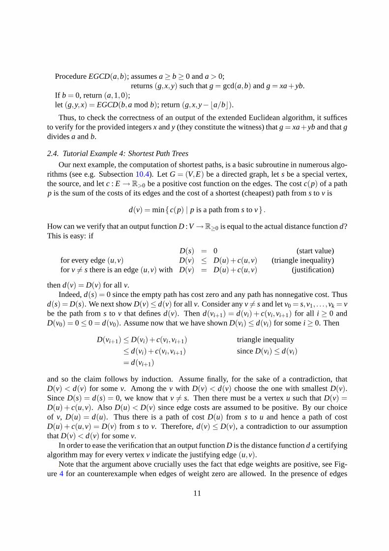
2.4. Tutorial Example 4: Shortest Path Trees

Our next example, the computation of shortest paths, is a basic subroutine in numerous algo-rithms (see e.g. Subsection10.4). Let G = (V,E) be a directed graph, lets be a special vertex,the source, and letc : E→ R>0 be a positive cost function on the edges. The costc(p) of a pathp is the sum of the costs of its edges and the cost of a shortest (cheapest) path froms to v is

d(v) = minc(p) | p is a path froms to v .

How can we verify that an output functionD :V→R≥0 is equal to the actual distance functiond?This is easy: if

D(s) = 0 (start value)for every edge(u,v) D(v) ≤ D(u)+c(u,v) (triangle inequality)for v 6= s there is an edge(u,v) with D(v) = D(u)+c(u,v) (justification)

thend(v) = D(v) for all v.Indeed,d(s) = 0 since the empty path has cost zero and any path has nonnegative cost. Thus

d(s) = D(s). We next showD(v)≤ d(v) for all v. Consider anyv 6= sand letv0 = s,v1, . . . ,vk = vbe the path froms to v that definesd(v). Thend(vi+1) = d(vi) + c(vi ,vi+1) for all i ≥ 0 andD(v0) = 0≤ 0 = d(v0). Assume now that we have shownD(vi)≤ d(vi) for somei ≥ 0. Then

D(vi+1)≤D(vi)+c(vi ,vi+1) triangle inequality

≤ d(vi)+c(vi ,vi+1) sinceD(vi)≤ d(vi)

= d(vi+1)

and so the claim follows by induction. Assume finally, for thesake of a contradiction, thatD(v) < d(v) for somev. Among thev with D(v) < d(v) choose the one with smallestD(v).SinceD(s) = d(s) = 0, we know thatv 6= s. Then there must be a vertexu such thatD(v) =D(u)+ c(u,v). Also D(u) < D(v) since edge costs are assumed to be positive. By our choiceof v, D(u) = d(u). Thus there is a path of costD(u) from s to u and hence a path of costD(u)+ c(u,v) = D(v) from s to v. Therefore,d(v) ≤ D(v), a contradiction to our assumptionthatD(v) < d(v) for somev.

In order to ease the verification that an output functionD is the distance functiond a certifyingalgorithm may for every vertexv indicate the justifying edge(u,v).

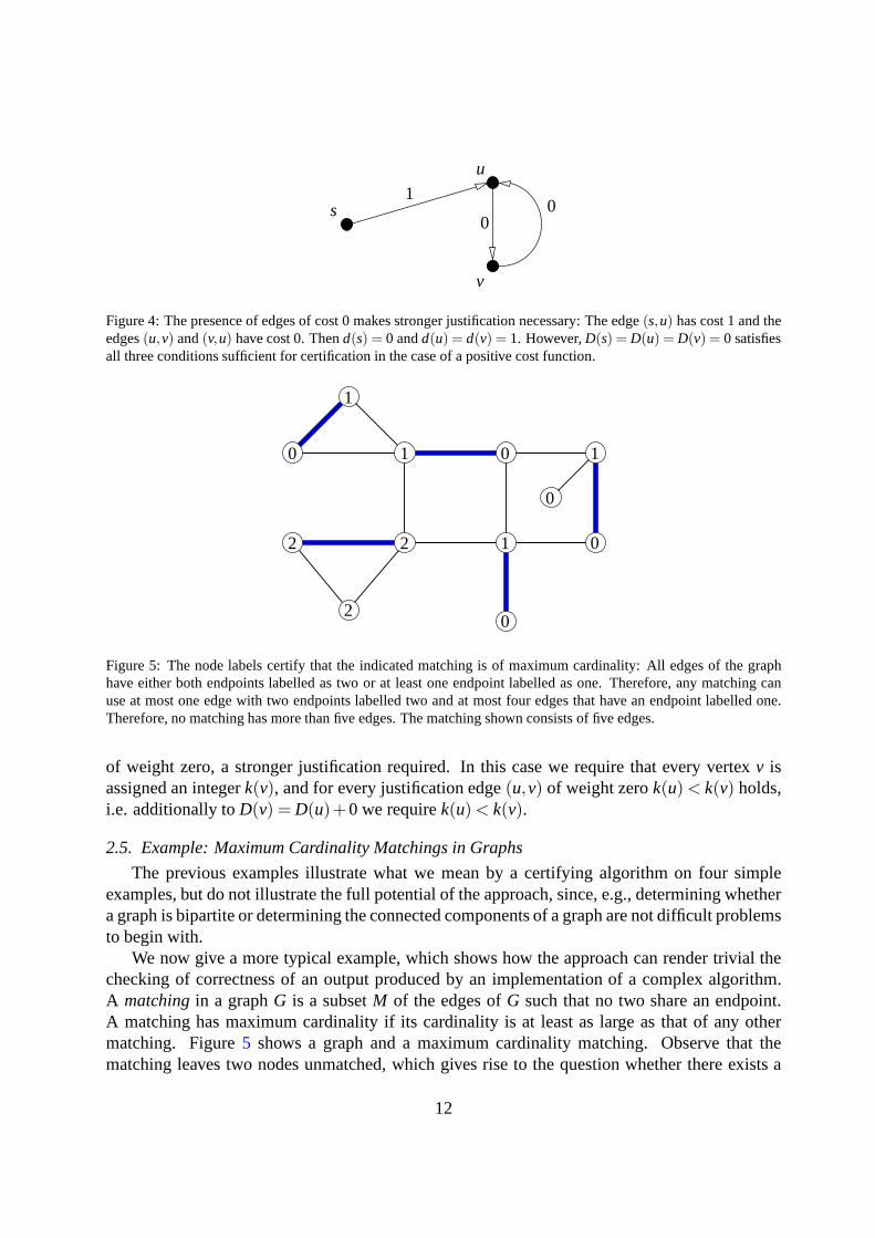
Note that the argument above crucially uses the fact that edge weights are positive, see Fig-ure 4 for an counterexample when edges of weight zero are allowed.In the presence of edges

11

s

u

v

1

00

Figure 4: The presence of edges of cost 0 makes stronger justification necessary: The edge(s,u) has cost 1 and theedges(u,v) and(v,u) have cost 0. Thend(s) = 0 andd(u) = d(v) = 1. However,D(s) = D(u) = D(v) = 0 satisfiesall three conditions sufficient for certification in the caseof a positive cost function.

0 1 0 1

012

0

2

2

1

0

Figure 5: The node labels certify that the indicated matching is of maximum cardinality: All edges of the graphhave either both endpoints labelled as two or at least one endpoint labelled as one. Therefore, any matching canuse at most one edge with two endpoints labelled two and at most four edges that have an endpoint labelled one.Therefore, no matching has more than five edges. The matchingshown consists of five edges.

of weight zero, a stronger justification required. In this case we require that every vertexv isassigned an integerk(v), and for every justification edge(u,v) of weight zerok(u) < k(v) holds,i.e. additionally toD(v) = D(u)+0 we requirek(u) < k(v).

2.5. Example: Maximum Cardinality Matchings in Graphs

The previous examples illustrate what we mean by a certifying algorithm on four simpleexamples, but do not illustrate the full potential of the approach, since, e.g., determining whethera graph is bipartite or determining the connected components of a graph are not difficult problemsto begin with.

We now give a more typical example, which shows how the approach can render trivial thechecking of correctness of an output produced by an implementation of a complex algorithm.A matchingin a graphG is a subsetM of the edges ofG such that no two share an endpoint.A matching has maximum cardinality if its cardinality is at least as large as that of any othermatching. Figure5 shows a graph and a maximum cardinality matching. Observe that thematching leaves two nodes unmatched, which gives rise to thequestion whether there exists a

12

matching of larger cardinality. What is a witness for a matching being maximum cardinality? Ed-monds [Edm65a, Edm65b] gave the first efficient algorithm for maximum cardinality matchings.The algorithm is certifying.

An odd-set cover OSCof G is a labeling of the nodes ofG with nonnegative integers suchthat every edge ofG is either incident to a node labeled 1 or connects two nodes labeled with thesame numberi ≥ 2.

Theorem 1 ([Edm65a]). Let N be any matching in G and let OSC be an odd-set cover of G. Forany i≥ 0, let ni be the number of nodes labeled i. Then

|N| ≤ n1+ ∑i≥2⌊ni/2⌋ .

Proof: For i, i ≥ 2, letNi be the edges inN that connect two nodes labeledi and letN1 be theremaining edges inN. Then

|Ni| ≤ ⌊ni/2⌋ and |N1| ≤ n1

and the bound follows.

It can be shown (but this is non-trivial) that for any maximumcardinality matchingM thereis an odd-set coverOSCwith

|M|= n1+ ∑i≥2⌊ni/2⌋, (1)

thus proving the optimality ofM. In such a cover allni with i ≥ 2 are odd, hence the name.The certifying algorithm for maximum cardinality matchingreturns a matchingM and an

odd-set coverOSCsuch that (1) holds. By the argument above, the odd-set cover proves theoptimality of the matching. Observe, that is itnot necessary to understand why odd-set coversproving optimality exist. It is only required to understandthe simple proof of Theorem1, show-ing that equation (1) proves optimality. Also, a correct program which checks whether a set ofedges is a matching and a node labelling is an odd-set cover which together satisfy (1) is easy towrite.

2.6. Case Study: The LEDA Planar Embedding Package

A planar embeddingof an undirected graphG is a drawing of the graph in the plane suchthat no two edges ofG cross and no edge crosses over a vertex. See Figure6 for an example. Agraph isplanar if it is possible to embed it in the plane in this way. Planar graphs were amongthe first classes of graphs that were studied extensively.

A faceof a planar embedding is a connected region of the plane that remains when points onthe embedding are removed. Letn be the number of vertices,m the number of edges, and letfbe the number of faces of a planar embedding. Euler gave what is known asEuler’s formulafora connected planar embedded graph:n+ f = m+2 (see Figure6).

The proof of this is frequently used as undergraduate exercise on induction on the numberof edges. As a base case,m= n−1, the graph is a tree, and an embedding of a tree always has

13

Figure 6: The depicted connected planar graph has 8 vertices, 5 faces (including the outer face), and thus 8+5−2=11 edges.

exactly one face. The formula holds. For the induction step,supposeG is a planar graph withm> n−1 and the formula holds for all planar embeddings of connected graphs with fewer thanmedges. Sincem> n−1, G has a cycle. Removal of an edge of the cycle in any planar embeddingof G causes two faces to merge, leavingn′ = n vertices,f ′ = f −1 faces, ande′ = e−1 edges.By the induction hypothesis, it holds thatn′+ f ′ = e′+2, which impliesn+ f = e+2, and theformula holds for the original planar embedding ofG.

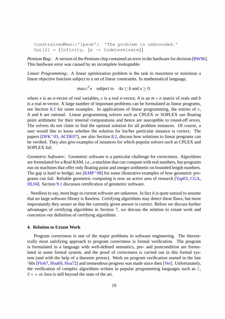
In the early 1900’s, there was an extensive effort to give acharacterizationof those graphsthat are planar. In 1920, Kuratowski gave what remains one ofthe most famous theorems ingraph theory: a graph is planar if and only if it has nosubdivisionof aK5 or aK3,3 as a subgraph(see Figure7). TheK5 is the complete graph on five vertices, theK3,3 is the complete bipartitegraph with three vertices in each bipartition class, and a subdivision of a graph is what is obtainedby repeatedly subdividing edges by inserting vertices of degree two on them.

The planarity test in the Library of Efficient Data Structures and Algorithms (LEDA), apopular package of implementations of many combinatorial and geometric algorithms [MN99,MN95], played a crucial role in the development of certifying algorithms and the developmentof LEDA.

There are several linear time algorithms for planarity testing [HT74, LEC67, BL76]. Animplementation of the Hopcroft and Tarjan algorithm was added to LEDA in 1991. The imple-mentation had been tested on a small number of graphs. In 1993, a researcher sent Mehlhorn andNaher a graph together with a planar drawing of it, and pointed out that the program declared thegraph non-planar. It took Mehlhorn and Naher some days to discover the bug.

More importantly, they realized that a complex question of the form “is this graph planar”deserves more than a yes-no answer. They adopted the thesis that

a program should justify (prove) its answers in a waythat is easily checked by the user of the program.

What does this mean for the planarity test?

14

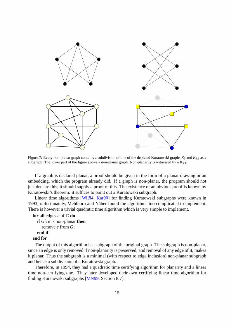
Figure 7: Every non-planar graph contains a subdivision of one of the depicted Kuratowski graphsK5 andK3,3 as asubgraph. The lower part of the figure shows a non-planar graph. Non-planarity is witnessed by aK3,3.

If a graph is declared planar, a proof should be given in the form of a planar drawing or anembedding, which the program already did. If a graph is non-planar, the program should notjust declare this; it should supply a proof of this. The existence of an obvious proof is known byKuratowski’s theorem: it suffices to point out a Kuratowski subgraph.

Linear time algorithms [Wil84, Kar90] for finding Kuratowski subgraphs were known in1993; unfortunately, Mehlhorn and Naher found the algorithms too complicated to implement.There is however a trivial quadratic time algorithm which isvery simple to implement.

for all edgeseof G doif G\e is non-planarthen

removee from G;end if

end forThe output of this algorithm is a subgraph of the original graph. The subgraph is non-planar,

since an edge is only removed if non-planarity is preserved,and removal of any edge of it, makesit planar. Thus the subgraph is a minimal (with respect to edge inclusion) non-planar subgraphand hence a subdivision of a Kuratowski graph.

Therefore, in 1994, they had a quadratic time certifying algorithm for planarity and a lineartime non-certifying one. They later developed their own certifying linear time algorithm forfinding Kuratowski subgraphs [MN99, Section 8.7].

15

Note that the proof of Kuratowski’s theorem, which is that a subdivision of aK5 or a K3,3always exists in a non-planar graph, is irrelevant to the protocol for convincing a user that a graphis non-planar. All that is needed is for the user to understand the following proof:

Lemma 2. A graph that contains a subdivision of K5 or K3,3 is non-planar.

Proof: Subdividing an edge cannot make a non-planar graph planar, so it suffices to show thatK5 andK3,3 are non-planar. Suppose there is a planar embedding ofK5. Each face touches at leastthree edges and each edge touches at most two faces. TheK5 has ten edges, so the number offaces is at most⌊(2/3) ·10⌋= 6. By Euler’s formula, 5+6≥ 10+2, a contradiction. Similarly,supposeK3,3 has a planar embedding. Since the graph is bipartite, the cycle around each facemust be even, so each face touches at least four edges and eachedge once again touches atmost two faces. The number of faces is at most⌊(2/4)9⌋ = 4. By Euler’s formula we obtain6+4≥ 9+2, a contradiction.

Let us now examine the checker. In the case of non-planarity,no matter how the Kuratowskisubgraph is found, a convenient certificate is obtained by returning it as sequences of edges. AK5 has ten edges, so if the Kuratowski subgraph is a subdivisionof aK5, it consists of ten disjointpaths sharing five ending vertices. The ending vertices are listed, and the ten paths are each givenas a sequence of edges, in order. The checker verifies that foreach pair of ending vertices there isa path with these vertices as beginning and end, cycling through the paths, checking and markingvertices along the way, to make sure that the paths are disjoint except at their endpoints. Thecheck of aK3,3 is similar.

Let us turn to witnesses of planarity. The obvious witness isa planar drawing. There isa drawback of using a planar drawing as the witness: It is non-trivial to check in linear timewhether a drawing is actually planar.

A less obvious form of witness is acombinatorial planar embedding, see Figure8. We firstexplain, what acombinatorial embeddingis. A combinatorial embedding uses twotwin directededges(u,v) and(v,u) for each undirected edge of the graph. These twins have pointers to eachother. For each vertexu of G, the edges incident to it are arranged in a circular linked listL(u). Acombinatorial embedding isplanar if there is a planar embedding ofG in which for each vertexu the counterclockwise order of the edges incident tou agrees with the cyclic order inL(u).

How does one verify whether a combinatorial embedding is planar? One simply checksEuler’s relation. A combinatorial embedding gives rise to adecomposition of the directed edgesinto a collection of cycles, calledboundary cycles. The boundary cycle containing a particulardirected edge(u,v) is defined as follows. Let(u,v) be a directed edge with twin(v,u) and let(v,u′) be the directed edge after(v,u) in the circular listL(v). Then(v,u′) is the next edge inthe boundary cycle containing(u,v), cf. Figure8. We continue in this way until we are back at(u,v). Why are we guaranteed to come back to where we started? To establish this, it suffices tonote that the edge preceding(u,v) in the boundary cycle is also uniquely defined. Let(u,v′) bethe edge before(u,v′) in L(u) and let(v′,u) be the twin of(u,v′). Then(v′,u) precedes(u,v) inthe boundary cycle containing it.

16

a b

c

d

evertex

counterclockwisecyclic adjacency list

a 〈b〉b 〈a,c,d〉c 〈d,b〉d 〈b,c,e〉e 〈d〉

Figure 8: A planar graph and the corresponding planar combinatorial embedding: For each vertex, the incidentedges are listed in counterclockwise order. The boundary cycles are(a,b),(b,d),(d,e),(e,d),(d,c),(c,b),(b,a)and(c,d),(d,b),(b,c). Observe that the successor of(d,e) is determined as follows: go to the twin(e,d) and thento the next edge in cyclic order, i.e.,(e,d).

Lemma 3. Let G be a connected graph with n> 1 vertices, and m edges. Then a combinatorialembedding of G with f boundary cycles is planarif and only if n+ f = m+2.

Proof: As before, we argue by induction on the number of edges. As a base case,m= n−1and the graph is a tree. Any combinatorial embedding of a treeis planar and gives rise to a singleboundary cycle; hencef = 1 andn+ f = m+2.

For the induction step, letI be a combinatorial embedding of a connected graphG with m>n−1 edges, and we assume by induction that the lemma applies to all combinatorial embeddingsof graphs withm−1 edges. Iff = 1, then the embedding cannot be planar, sinceG has a singleboundary cycle and any planar drawing has more than one face in accordance with the fact thatn+ f = m+2 does not hold.

Supposef ≥ 2. We claim that there must be an edgee= (u,v),(v,u) such that(u,v) and(v,u) lie on different boundary cycles; otherwise, the edges in cyclic order around each vertexare forced to be in the same boundary cycle, and sinceG is connected, there is only one boundarycycle, a contradiction. LetG′ = G−e and letI ′ be the combinatorial embedding ofG′ obtainedby removinge from I . This merges two boundary cycles into one, call itC, soI ′ has f ′ = f −1boundary cycles,m′ = m−1 edges, andn′ = n vertices. By basic algebra,I ′ satisfies the formulaif and only if I does. By the induction hypothesisI ′, henceI , satisfies the formula if and only ifI ′ is planar. IfI ′ is not planar, then neither isI , sinceI ′ is a subembedding. IfI ′ is planar, thenC is the boundary of a face, sayF, in some planar drawingD′ of G′ corresponding toI ′. Sinceu andv are onC, F can be subdivided inD′ by drawing the edgeu,v so that it is internal toFexcept at its endpoints. This yields a planar drawingD corresponding toI , soI is planar.

So in the case of a planarity a convenient witness is a combinatorial embedding ofG. Thechecker determines the numberf of boundary cycles of the combinatorial embedding and acceptsthe combinatorial embedding ifn+ f = m+2.

The example illustrates that the reason why a certificate always exists (the proof of Kura-towski’s theorem in this case) is irrelevant to the protocolfor convincing a user that a particularoutput is correct. All that is needed is for the user to understand the proofs of Lemmas2 and3.

17

What does the case study performed in this section illustrate about the current state of algo-rithm design and software engineering? The algorithm on which the program was based is well-known to be correct. Obviously, the programmer made a mistake in implementing it. However,another problem was that users were willing to accept a declaration that a graph was non-planar,based partly on the knowledge that it was based on an algorithm that is well-known to be correct.

Additionally, another problem was that the designers of algorithms traditionally considertheir work done when they have produced a proof that their algorithm never produces an incor-rect output. It has gone unrecognized in the algorithm-design community that, in view of theimplementation obstacles, algorithm design should also assist the process of obtaining a correctimplementation.

3. Examples of Program Failures

To emphasize the importance of methods that facilitate reliability of computation, we givesome examples of failures in algorithmic software. The failures are either bugs or due to theuse of approximate arithmetic. The first kind of failure shows that even in prevalent, widelydistributed programs software bugs have historically appeared. Of course, once bugs becomeknown, they are repaired and hence the bugs reported here do no longer exist in the currentversion of the programs.

Planarity Test in LEDA 2.0:.As extensively illustrated in Subsection2.6, the planarity test inLEDA 2.0 was incorrect. It declared some planar graphs non-planar. Mehlhorn and Naher cor-rected the error in LEDA 2.1 and made the planarity test certifying. This was their first use of acertifying algorithm. However, the first solution was far from satisfying, as the running time ofthe certifying algorithm was quadratic compared to linear time for the non-certifying algorithm.It took some time to develop an equally efficient certifying algorithm.

Triconnectivity of Graphs:.A connected graph is triconnected if the removal of any pair ofvertices does not disconnect it. There are linear-time algorithms for deciding triconnectivity ofgraphs [HT73, MR92]. Gutwenger and Mutzel [GM00] implemented the former algorithm andreported that some non-triconnected graphs are declared triconnected by it. They provided acorrection. We come back to this problem in Section9.8.

Constrained Optimization in Mathematica 4.2:.Version 4.2 of Mathematica (a software environ-ment for mathematical computation) fails to solve a small integer linear program; the example isso small that we can give the full input and output. The first problem asks to compute the mini-mum of the functionx subject to the constraintsx = 1 andx = 2. The system returns the optimalvalue is 2 and that the substitutionx→ 2 attains it. The second problems asks to maximize thefunction under the same constraints. The system answers that the optimal value is infinite andthatx has an indeterminate value in this solution.

In[1] := ConstrainedMin[ x , x==1,x==2 , x ]Out[1] = 2, x->2In[1] := ConstrainedMax[ x , x==1,x==2 , x ]

18

ConstrainedMax::"lpsub": "The problem is unbounded."Out[2] = Infinity, x -> Indeterminate

Pentium Bug:.A version of the Pentium chip contained an error in the hardware for division [BW96].This hardware error was caused by an incomplete lookuptable.

Linear Programming:.A linear optimization problem is the task to maximize or minimize alinear objective function subject to a set of linear constraints. In mathematical language,

maxcTx subject to Ax≤ b andx≥ 0.

wherex is ann-vector of real variables,c is a realn-vector,A is anm×n matrix of reals andbis a realm-vector. A large number of important problems can be formulated as linear programs,see Section8.2 for some examples. In applications of linear programming, the entries ofc,A and b are rational. Linear programming solvers such as CPLEX or SOPLEX use floatingpoint arithmetic for their internal computations and henceare susceptible to round-off errors.The solvers do not claim to find the optimal solution for all problem instances. Of course, auser would like to know whether the solution for his/her particular instance is correct. Thepapers [DFK+03, ACDE07], see also Section8.2, discuss how solutions to linear programs canbe verified. They also give examples of instances for which popular solvers such as CPLEX andSOPLEX fail.

Geometric Software:.Geometric software is a particular challenge for correctness. Algorithmsare formulated for a Real RAM, i.e., a machine that can compute with real numbers, but programsrun on machines that offer only floating point and integer arithmetic on bounded length numbers.The gap is hard to bridge; see [KMP+08] for some illustrative examples of how geometric pro-grams can fail. Reliable geometric computing is now an active area of research [Yap03, CGA,HL04]. Section9.1discusses certification of geometric software.

. Needless to say, most bugs in current software are unknown. In fact it is quite natural to assumethat no large software library is flawless. Certifying algorithms may detect these flaws, but moreimporatantly they assure us that the currently given answeris correct. Before we discuss furtheradvantages of certifying algorithms in Section7, we discuss the relation to extant work andconcretize our definition of certifying algorithms.

4. Relation to Extant Work

Program correctness is one of the major problems in softwareengineering. The theoret-ically most satisfying approach to program correctness is formal verification. The programis formulated in a language with well-defined semantics, pre- and postcondition are formu-lated in some formal system, and the proof of correctness is carried out in this formal sys-tem (and with the help of a theorem prover). Work on program verification started in the late’60s [Flo67, Hoa69, Hoa72] and tremendous progress was made since then [Ver]. Unfortunately,the verification of complex algorithms written in popular programming languages such asC,C++ or Java is still beyond the state of the art.

19

Program testing is the most widely used approach to program correctness, see [Zel05] for arecent account. A list of correct input/output pairs(xi ,yi) is maintained. A program is acceptedif, for eachxi on the list, it produces the correspondingyi . The common objections against testingare that it can prove the presence of errors, but never their absence, and that a program can onlybe tested on inputs for which the correct output is already known by other means.

It has been known since the 1950’s that linear programming duality [Chv93, Sch03] providesa method for checking the result of linear programs. In a pairof solutions(x,x), one for a linearprogram and one for its dual, both solutions are optimal if and only if they have the same objectivevalue, see Subsection8.2. A special case of linear programming duality is the max-flow-min-cuttheorem for network flows.

Sullivan and Masson [SM90, SM91, BS95, BSM95, SWM95, BS94] introduced the conceptof a certification trail for checking. The idea is that a program leaves a trail of information thatcan be used to check whether it worked correctly. They applied the idea mainly to data structures.In later work [BSM97], they combined certification trails with formal verification. We discusschecking of data structures in Section12. Certification trails catch errors ultimately, but notimmediately.

Blum and Kannan [BK89, BK95] started a theory of program checking; see [Blu93, BW94,BLR90, WB97, BW96] for follow-up work. Given a programP allegedly computing a func-tion2 f , how can one check whetherP(x0) = f (x0) for a particular inputx0. A checkerCis a probabilistic expected-polynomial-time oracle machine (it usesP as a subroutine) withthe property: ifP(x) = f (x) for all x, thenC on input x0 accepts with high probability. IfP(x0) 6= f (x0), C on inputx0 rejects with high probability. IfP(x0) = f (x0), but P 6= f , thechecker may accept or reject. They describe, among others, checkers for graph isomorphism, theextended gcd, and sorting reals. In [BLR90] the concept is generalized to self-correcting algo-rithms. For example, assumeadd is a function that correctly adds for most pairs of inputs. Thenadd(x,y) = add(add(x, r),add(y,−r)), wherer is a random number, correctly adds all pairs withnonzero probability, since the concrete additionx+y is replaced by three random additions.

There are essential differences between certifying algorithms and the work by Blum et al.First, they mention but do not explore that adding additional output (= our witness) may easethe life of the checker; they give the extended gcd and maximum flow as examples. In contrast,we insist that certifying programs return witnesses that prove the correctness of their output.In exceptional cases, the witness may be trivial. The secondessential difference is that theyallow checkers to be arbitrarily complex programs (as long as they are polyomial-time) andnevertheless assume checkers to be correct. In constrast, we insist that checkers are simpleprogram and assume that only the simplest programming taskscan be done without error; seeSubsection6.1.

Our approach has already shown its usefulness in the LEDA project [LED]. At the time ofthis writing, LEDA contains checkers for all network and matching algorithms (mostly based onlinear programming duality), for various connectivity problems on graphs, for planarity testing,for priority queues, and for the basic geometric algorithms(convex hulls, Delaunay diagrams,

2They consider only programs with trivial preconditions

20

and Voronoi diagrams). Program checking has greatly increased the reliability of the implemen-tations in LEDA. There are many other problems for which certifying algorithms are known. Wereview some of them in the sections to come and give a guide to the literature in Subsection9.8.

Proof-carrying code [NL96, Nec97] is a “mechanism by which a host system can determinewith certainty that it is safe to execute a program supplied by an untrusted source. For this tobe possible, the untrusted code producer must supply with the code a safety proof that attests tothe code’s adherence to a previously defined safety policy. The host can then easily and quicklyvalidate the proof (quote from [Nec97])”. We will use methods akin to proof-carrying code inSection5.

An interactive proof system [GMR89] is a protocol that enables a verifier to be convicedby a prover of some output via a series of message exchanges. In the language of certifyingalgorithms, their execution needs a bidirectional communication between the checker and thecertifying algorithm. However, to be in accordance with therequirements we pose onto certifyingalgorithms, further simplicity constraints have to be introduced. If done so, they constitute anextension of certifying algorithms that carries several, but not all of the advantages of certifyingalgorithms mentioned in Section7.

5. Definitions and Formal Framework

We consider algorithms taking an input from a setX and producing an output in a setY. Theinputx∈ X is supposed to satisfy a precondition3 ϕ(x) and the input together with the outputy∈Y is supposed to satisfy a postconditionψ(x,y). Hereϕ : X→T,F andψ : X×Y→T,F .We call the pair(ϕ,ψ) an I/O-specificationor an I/O-behavior.

In the case of graph bipartition for example, we haveY = bipartite,nonbipartite. Withrespect toX, we can take different standpoints. As an algorithm designer or a programmer usinga strongly typed programming language, we could takeX as the set of all finite undirected graphs.Thenϕ(x) = T for all x∈ X andψ(x,y) = T iff

x is a bipartite graph andy = bipartite orx is a non-bipartite graph andy = nonbipartite.

As a programmer using Turing machines or an untyped programming language, we would takeX as the set of all conceivable inputs, sayΣ∗ in the case of Turing machines or all memorystates in the case of the untyped programming language. Thenϕ(x) = T iff x is the well-formedrepresentation of an undirected graph andψ(x,y) = T iff the precondition is true and

x represents a bipartite graph andy = bipartite orx represents a non-bipartite graph andy = nonbipartite.

In all examples considered in this paper, it is easy to check whether representations are well-formed. We can therefore safely ignore the issue of input representation in most of our discus-sions.

3For a predicateP : X→T,F , we use “x satisfiesP” or P(x) = T interchangeably. Similarly, we useP(x) = Fandx does not satisfyP interchangeably. In formulae we writeP(x) for P(x) = T and¬P(x) for P(x) = F .

21

We specifically allow the possibility that a pair(x,y) of input and output satisfies the post-condition, even thoughx does not satisfy the precondition. We will next define three kinds ofcertifying algorithms: strongly certifying, certifying,and weakly certifying algorithms. In thecase of a trivial precondition, i.e.,ϕ(x) = T for all x, the three notions coincide.

5.1. Strongly Certifying Algorithms

Strongly certifying algorithms are the most desirable kindof algorithm. On every input, astrongly certifying algorithm proves to its users that it worked correctly or that the user providedit with an illegal input; it also says which of the two alternative holds. More precisely, for anyinputx, it either produces a witness showing thatx does not satisfy the precondition or it producesan outputy and a witness showing that the pair(x,y) satisfies the postcondition. For technicalreasons, in the first case, we want the algorithm to also produce an answering output, in additionto the witness. We could have it return an arbitrary output but find it more natural to extend theoutput setY by a special symbol⊥ and use⊥ as an indicator for a violated precondition. We callY⊥ := Y∪⊥ theextended output set. We useW to denote the set of witnesses.

A strong witness predicatefor an I/O-specification(ϕ,ψ) is a predicateW : X×Y⊥×W→T,F with the following properties:

Strong witness property: Let (x,y,w) ∈ X×Y⊥×W satisfy the witness predicate. Ify =⊥, wproves thatx does not satisfy the precondition and ify∈Y, w proves that(x,y) satisfies thepostcondition, i.e.,

∀x,y,w (y =⊥ ∧W (x,y,w)) =⇒ ¬ϕ(x) and(y∈Y∧W (x,y,w)) =⇒ ψ(x,y)

(2)

Checkability: For a triple(x,y,w) it is trivial to determine the valueW (x,y,w).

Simplicity: The implications (2) have a simple proof.

For the moment, we want to leave the checkability and the simplicity property informalnotions. We invite the reader to check our examples against his/her notion of simplicity andcheckability. We discuss this further in Subsection5.5.

A strongly certifying algorithmfor I/O-specification(ϕ,ψ) and strong witness predicateWis an algorithm with the following properties:

• It halts for all inputsx∈ X.

• On inputx∈ X it outputs ay∈Y⊥ and aw∈W such thatW (x,y,w) holds.

We illustrate the definition with two examples. The first example is the test for bipartitenessalready used in the introduction. Here,X is the set of all undirected graphs and the preconditionis trivial. Any graph is a good input. The output set isY = YES,NO. If the output is YES,the witness is a 2-coloring, if the output is NO, the witness is an odd cycle.

Next, we give an example, where the precondition is non-trivial. We describe a stronglycertifying algorithm that five-colors any planar graph. Thealgorithm does not decide planarity.

22

So X is the set of undirected graphs. We useG to denote an input graph. The precondition isthatG is planar. For a planar graphG = (V,E), the algorithm is supposed to color the verticesof G with five colors such that any two adjacent vertices have distinct colors, i.e., the algorithmconstructs a mappingc : V → 1,2,3,4,5 such that for any edgee= (u,v) ∈ E, c(u) 6= c(v).For a non-planar graph, the algorithm will either prove non-planarity or provide a 5-coloring.Non-planarity is proven by exhibiting a sequence of planarity preserving transformations thattransform the input graph to a graph that is clearly non-planar. Consider the following recursivealgorithm. IfG has at most five vertices, the algorithm returns a coloring. So assume thatG hasmore than five vertices. IfG has more than 3n−6 edges, the algorithm declares the graph non-planar. The witness is the number of edges. IfG has at most 3n−6 edges,G must have a vertexof degree five or less. Letv be such a vertex. Ifv has degree four or less, the algorithm removesv from the graph and calls itself onG− v. Clearly, removal of a vertex preserves planarity. Ifthe recursive call returns a five coloring, it is easily extended toG. If v has degree five, considerthe neighbors ofv. If the neighbors ofv form a K5, return it as a witness for non-planarity.Otherwise, there must be two neighbors, sayx andy, that are non-adjacent. Removev from thegraph, identifyx andy, and remove any parallel edges this may create. It is crucialto observehere that removal ofv and identification ofx andy, does not destroy planarity. This is easy tosee by conceptualizing a planar drawing and performing the operation there. If the recursivecall returns a five-coloring, it is easy to extend it toG. We use forx andy the color that wasgiven to their contraction in the smaller graph and we give a color that was not used on theneighbors ofv for v. In this way, we either find a coloring of the input graphG or a sequenceof planarity preserving reductions to a graphG′ that is clearly non-planar; either because it hastoo many edges or because it contains aK5. For any planar graph, the algorithm will produce afive-coloring. It also will produce five-colorings of some non-planar graphs. For example, it willcolor aK5. If the algorithm fails to find a five-coloring, it produces a witness that the input graphis non-planar. Note that the algorithm does not decide whether the precondition (that the graphis planar) was met.

5.2. Certifying Algorithms

In some situations, we have to settle for less. The algorithmwill only prove that either theprecondition is violated or the postcondition is satisfied.It will, in general, not be able to alsoindicate which of the alternatives holds.

As an example, consider binary search. Its input is a numberz and an arrayA[1..n] of num-bers. The precondition states thatA is sorted in increasing order. The search outputs YES, ifz isstored in the array, and it outputs NO, ifz is not stored in the array. In the former case, a witness isan indexi such thatA[i] = z, in the latter case, a witness is an indexi such thatA[i−1] < z< A[i];hereA[0] =−∞ andA[n+1] = +∞ for convenience. Binary search maintains two indicesℓ andrwith A[ℓ] < z< A[r] andℓ < r. Initially, ℓ = 0 andr = n+1. As long asr > ℓ+1, it comparesz with A[m], wherem= ⌊(r + ℓ)/2⌋. If z= A[m], the algorithms stops. Ifz< A[m], r is set tom and the algorithms continues. Ifz> A[m], ℓ is set tom and the algorithm continues. Observethat binary search does not discover any violation of its precondition. In fact discovering allviolations would require linear time in general. This example leads us to the definition of an(ordinary) certifying algorithm:

23

A witness predicatefor an I/O-specification(ϕ,ψ) is a predicateW : X×Y⊥×W→T,F with the following properties:

Witness property: Let (x,y,w) satisfy the witness predicate. Ify =⊥, w proves thatx does notsatisfy the precondition. Ify∈Y, w proves thatx does not satisfy the precondition or(x,y)satisfies the postcondition, i.e.,

∀x,y,w (y =⊥ ∧W (x,y,w)) =⇒ ¬ϕ(x) and(y∈Y∧W (x,y,w)) =⇒ ¬ϕ(x)∨ψ(x,y)

(3)

The second implication may also be written asy∈Y∧ϕ(x)∧W (x,y,w) =⇒ ψ(x,y).

Checkability: For a triple(x,y,w) it is trivial to determine the valueW (x,y,w).

Simplicity: The implications (3) have a simple proof.

In the case of binary search,X is the set of pairs(A,z) whereA is an array of numbers andzis a number,Y is YES,NO andW is 0..n. For(A,z) ∈ X, y∈Y⊥ andw∈W, we have

W (x,y,w) = T iff

y = YES∧w = i ∈ 1..n∧z= A[i] or

y = NO∧w = i ∈ 0..n∧A[i] < z< A[i +1]

A certifying algorithmfor I/O-specification(ϕ,ψ) and witness predicateW is an algorithmP with the following properties:

• It halts for all inputsx∈ X.

• On inputx∈ X it outputs ay∈Y⊥ and aw∈W such thatW (x,y,w) holds.

5.3. Weakly Certifying Algorithms

Sometimes, we have to settle for even less. Aweakly certifying algorithmfor I/O-specification(ϕ,ψ) and witness predicateW is an algorithm with the following properties:

• It halts for all inputsx∈ X satisfying the precondition. For inputs not satisfying thepre-condition, it may or may not halt.

• If it halts on inputx∈ X, it outputs ay∈Y⊥ and aw∈W such thatW (x,y,w) holds.

As an example, consider a naive randomized SAT-solver: It isgiven a formulax, of which itis supposed to prove satisfiability. In other words our precondition is

ϕ(x) = (x is a satisfiable boolean formula) .

It tries random assignments until is has found a satisfying assignmentw. It then outputsy= YES,together withw as a witness. Checking the satisfiability ofx is trivial; w proves it. This algo-rithm is certifying, however since it does not halt on unsatisfiable input clauses it is only weaklycertifying. A more sophisticated example is the random SAT-solver analyzed by Moser [Mos09],which finds satisfying assignments of certain sparse SAT-clauses in polynomial time.

24

Theorem 2. Let (ϕ,ψ) be an I/O-specification. A certifying decision algorithm for ϕ plus aweakly certifying algorithm for behavior(ϕ,ψ) can be combined to a strongly certifying algo-rithm for behavior(ϕ,ψ).

Proof: Let x be any input. We first run the certifying decision algorithm for ϕ. It returnsy= ϕ(x) ∈ T,F and a witnessw certifying the correctness of the output. Ify is F, we return⊥andw as a witness for¬ϕ(x). If y is T, we run the weakly certifying algorithm for I/O-behavior(ϕ,ψ) on x. Sinceϕ(x), the algorithm returns ay′ with ψ(x,y′) and a witnessw′ certifying thecorrectness of the output. We returny′ andw′.

5.4. Efficiency

We call a certifying algorithmP efficientif there is an accompanying checkerC, such thatthe asymptotic running of bothP andC is at most the running time of the best known algorithmsatisfying the I/O-specification. All examples we have treated so far are efficient. We now givean example, where no efficient certifying algorithm is known. The 3-connectedness problem askswhether a graph may be disconnected by removing two vertices. Linear time algorithms [HT73,MR92] for this problem are known, but none of them is certifying.

Certifying that a graph is not 3-connected is simple, it suffices to provide a setSof vertices,|S| ≤ 2, such thatG\S is not connected. To certify that their removal disconnectsthe graph wecan, for example, use the algorithm that certifies the connected components (see Subsection2.2).Thus, we now focus on 3-connected graphs and describe anO(n2) algorithm that certifies 3-connectivity (a different certifyingO(n2) algorithm can be found in [Sch10]). We omit detailson how to find a separating set during the execution of the algorithm, in case the input graph isnot 3-connected. As certificate for 3-connectivity we will use a sequence of edge contractionsresulting in theK4, the complete graph on 4 vertices. Thecontractionof an edgee= xy of agraphG is the graphG/e obtained by replacingx andy with a single vertex, whose neighborsareN(x)∪N(y)\x,y. We call an edgeeof a 3-connected graphG contractibleif the contractedgraphG/e is 3-connected. A separating pair is a pair of vertices whoseremoval disconnects thegraph.

Lemma 4. Let e= (x,y) be an edge of a simple graph G whose end-vertices have a degreeof atleast3. If G/e is 3-connected, then G is 3-connected.

Proof: Since contractions cannot connect a disconnected graph, the original graphG is con-nected. There are no cut-vertices inG, as they would map to cut-vertices inG/e.

Any separating pair ofG must contain one of the end-vertices of edgee. Otherwise the pairis also separating inG/e. It cannot contain bothx andy, otherwise the contracted vertexxy isa cut-vertex inG/e. It suffices now to show thatx,u, with u∈V(G) \ y is not a separating pair.Suppose otherwise, then the graphG−x,u is disconnected, but the graphG−x,y,u is not.Thusy is a component ofG−x,u. But this is a contradiction sincey has degree at least 3in G.

25

To certify the 3-connectivity of a graphG, it thus suffices to provide a sequence of edgeswhich, when contracted in that order, have endpoints with a degree of a least 3 and whose con-traction results in aK4. We call such a sequence aTutte sequence. We now focus on how to findthe contraction sequence, given a 3-connected graph.

TheO(n2) algorithm needs three ingredients: First we require theO(n2) algorithm by Nag-amochi and Ibaraki [NI92] that finds a sparse spanning 3-connected subgraph ofG with at most3n−6 edges. Second we require a linear time algorithm for 2-connectivity. Third we require astructure theorem, that shows how to determine a small candidate set of edges among which wefind a contractible edge.

Theorem 3 (Krisell [Kri02 ]). If no edge incident to a vertex v of a 3-connected graph G iscontractible, then v has a least four neighbors of degree 3, which each are incident with twocontractible edges.

Consider now a vertexv of minimal degree in a 3-connected graph. If it has degree three, itcannot have four neighbors of degree three and hence must have an incident contractible edge.If it has degree four or more, it cannot have a neighbor of degree three (because otherwise, itsdegree would not be minimal) and hence must have an incident contractible edge. Also note thatan edgexy in a 3-connected graph is contractible, ifG−x,y is 2-connected.

We explain how to find the firstn/2 contractions in timeO(n2). By repeating the procedurewe obtain an algorithm that has overall a running time ofO(n2).

First use the algorithm by Nagamochi and Ibaraki [NI92]. The resulting graph has 3n−6edges. Thus while performing the firstn/2 contractions, there will always be a vertex withdegree at most 2·2 ·3 = 12. Choosing a vertex of minimal degree, we obtain a set of at most 12candidate edges, one of which must be contractible. To test whether an edgexy is contractible,we check whetherG−x,y is 2-connected with some linear time algorithm for 2-connectivity.

Theorem 4 ([Sch10]). A Tutte sequence for a 3-connected graph can be found in time O(n2).

It remains a challenge to find a linear time certifying algorithm for 3-connectivity of graphs.A linear time certifying algorithm for graphs 3-connectivity of Hamiltonian graphs was recentlyfound [EMS10]; it assumes that the Hamiltonian cycle is part of the input.

Efficiency and Usefulness:.For some problems, e.g., testing bipartiteness, maximum flow, match-ings, and min-cost flows, the best known algorithms are certifying and the cost of checking thewitness is negligible compared to the cost of computing it. For such programs, it is best to in-tegrate the checker into the program. For other problems, e.g., planarity testing, certificationincreases running time by a non-negligible multiplicativefactor (more than 2 and less than 10).Finally, there are problems, such as triconnectivity, where the best known certifying algorithmhas worse asymptotic complexity than the best known non-certifying algorithm. Even for thelatter kind of problem, certification is useful for two reasons. First, one can use the certifyingversion to generate test instances for the non-certifying version, and second, for small instancesthe slow certifying version may be fast enough.

26

5.5. Simplicity and Checkability

The definition of a certifying algorithm and its variants involve two non-mathematical termsthat we have not made precise: simplicity and checkability.They guarantee that it is “easy tocheck” whether a witnessw shows that an output is correct for a given input. We now elaborateon these terms.

Checkability:. Given x, y, andw, we require that it is trivial to determine whetherW (x,y,w)holds. We list a number of conceivable “formalizations” of “being trivial to determine”.

• There is a decision algorithm forW that runs in linear time.

• W has a simple logical structure. For example, we might require thatx, y, andw arestrings, thatW is a conjunction ofO(|x|+ |y|+ |w|) elementary predicates and that eachpredicate tests a simple property of relatively short substrings.

• There is a simple logical system, in which we can decide whetherW (x,y,w) holds.

• The correctness of a program decidingW (x,y,w) is obvious or can be established by anelementary proof.

• We can formally verify the correctness of the program decidingW (x,y,w).

Most witness predicates discussed in this article satisfy all definitions above. In Section6 wefurther investigate checkers, i.e., programs that determine the value of a witness predicateW .

Simplicity:. The witness property is easily verified, i.e., the (equivalent) implications

∀x,y,w W (x,y,w)→ ψ(x,y) (4)

∀x,y ¬ψ(x,y)→6 ∃w W (x,y,w) . (5)

have an elementary proof. Here, we assumed that the precondition is trivial. For the case of anon-trivial precondition, either statement (2) or (3) should have an elementary proof (the formerin the case of a strongly certifying algorithm, the latter inthe other cases). We find that all witnesspredicates discussed in this article fulfill the simplicityproperty.

Observe that we make no assumption about the difficulty of establishing the existence of awitness. In the case of a strongly certifying or certifying algorithm, this would be the statement

∀x ∃y,w W (x,⊥,w)∨W (x,y,w) .

In the case of a weakly certifying algorithm this would be thestatement

∀x ϕ(x) =⇒ (∃y,w W (x,⊥,w)∨W (x,y,w)) .

Indeed, the existence of witnesses is usually a non-trivialmathematical statement, and its com-putation a non-trivial computational task. For example, itis non-trivial to prove that a non-planargraph necessarily contains a Kuratowski subgraph (Subsection 2.5) and is non-trivial to prove

27

that a maximum matching can always be certified by an odd-set cover (Subsection2.6). Fortu-nately, a user of a certifying algorithm does not need to understand why a witness exists in allcases. He only needs to convince himself that it is easy to recognize witnesses and that a witness,indeed, certifies the correctness of the algorithm on the given instance.

The “definition” above rules out some obviously undesirablesituations:

1. Assume we have a complicated programP for I/O-behavior(ϕ,ψ). We could takew asthe record of the computation ofP on x and defineW (x,y,w) as “w is the computation ofP on inputx andy is the output of this computation”. IfP is correct, thenW is a witnesspredicate. This predicate certainly satisfies the checkability requirement. However, it doesnot satisfy the simplicity requirement, since a proof of thewitness property is tantamountto proving the correctness ofP.

2. Another extreme is to defineW (x,y,w) as “ψ(x,y)”. For this predicate simplicity is triv-ially given. However, decidingW amounts to a solution of the original problem.

As our definition is not and cannot be made mathematically stringent, whether an algorithmshould be accepted as certifying is a matter of taste. However, if we drop our non-mathematicalrequirement of “easiness to check”, we can ask formal questions on the existence of certifyingalgorithms.

Question 1. Does every computable function have a certifying algorithm.

A more stringent version of this question asks, in addition,about the resource requirementsof the certifying program.

Question 2. Does every program P have an efficient strongly certifying orcertifying or weaklycertifying counterpart, i.e., a counterpart with essentially the same running time?

More precisely, letP be a program with I/O-behavior(ϕ,ψ). An efficient strongly certifyingcounterpart would be a programQ and a predicateW such that

1. W is a strong witness predicate for(ϕ,ψ).

2. On inputx, programQ computes a triple(x,y,w) with W (x,y,w).

3. On inputx, the resource consumption (time, space) ofQ on x is at most a constant factorlarger than the resource consumption ofP.

For an ordinary certifying counterpart, we would replace strong witness predicate by witnesspredicate in the first condition. For a weakly certifying counterpart, we would additionally re-place the second condition by the following: ifQ halts onx, it computes a triple(x,y,w) withW (x,y,w), and ifϕ(x) thenQ halts onx. We address these questions in the next two subsections.

28

5.6. Deterministic Programs with Trivial Preconditions

We show that every deterministic program that has a trivial preconditionϕ(x) = T for all xcan be made certifying with only a constant overhead in running time. This sounds like a verystrong result. It is not really; the argument formalizes theintuition that a formal correctnessproof is a witness of correctness. The construction shows some resemblance to proof-carryingcode [NL96].

Let ψ be a postcondition and letP be a program (in a programming languageL with well-defined semantics) with I/O-behavior(T,ψ). We assume that we have a proof (in some formalsystemS) of the fact thatP realizes(T,ψ), i.e., a proof of the statement4

∀x P halts on inputx andψ(x,P(x)) . (6)

We usew2 to denote the proof.We extendP to a programQ which on inputx outputsP(x) and a witnessw = (w1,w2,w3)

wherew1 is the program textP, w2 is as above, andw3 is the computation ofP on inputx.The witness predicateW (x,y,w) holds if w has the required format, i.e.,w = (w1,w2,w3),

wherew1 is the program text of some programP, w2 is a proof inS thatP realizes I/O-behavior(T,ψ), w3 is the computation ofP on inputx, andy is the output ofw3. The following statementsshow that algorithmQ is an efficient certifying algorithm:

1. W is a strong witness predicate for I/O-behavior(T,ψ):

• Checkability: The check whether a triple(x,y,w) satisfies the witness predicate iseasy. We use a proof checker for the formal systemS to verify thatw2 is a proof forstatement (6). We use an interpreter for the programming languageL to verify thatw3 is the run ofP on inputx and thaty = P(x).

• Strong witness property and Simplicity:The proof of the implicationW (x,y,w)⇒ψ(x,y) is elementary: AssumeW (x,y,w). Thenw = (w1,w2,w3), wherew1 is theprogram text of some programP, w2 is a proof (in systemS) that P realizes I/O-behavior(T,ψ), w3 is the computation ofP on inputx, andy is the output ofw3.Thusy = P(x) andψ(x,P(x)).

2. For every inputx algorithmQ computes a witnessw with W (x,P(x),w). This follows fromthe definition ofQ.

3. The running time ofQ is asymptotically no larger than the running time ofP. The sameholds true for the space complexity. Observe thatQ produces a large output; however, theworkspace requirement is the same as forP. The same is true for the checker described inthe checkability argument.

We summarize the discussion.

4We useP(x) to denote the output ofP on inputx.

29

Theorem 5. Every deterministic program forI/O-specification(T,ψ) has an efficient stronglycertifying counterpart. This assumes that a proof for (6) in a formal system is available.

We admit that the construction above leaves much to be desired. It is not a practical way ofconstructing certifying algorithms. After all, certifying programs are an approach to correctnesswhen a formal correctness proof is out of reach. A frequent reaction to Theorems5 and7 is thatthey contradict intuition. In fact, we also started out wanting to prove the opposite. In an attemptto prove that some algorithms cannot be certifying without loss of efficiency, we discoveredTheorem5. We come back to this point in Section14.

However, the construction is also quite assuring and gives strong moral support. Every deter-ministic program can be made certifying with only a constantloss in time and space.So, whensearching for a certifying algorithm we only have to try hardenough; we are guaranteed to suc-ceed. The construction also captures the intuition that certification is no harder than a formalcorrectness proof of a program.

5.7. Non-Trivial Preconditions

For non-trivial preconditions the situation is more subtle. We will see that there are I/O-behaviors that can be realized by a non-certifying algorithm but cannot be realized by a certifyingalgorithm. However, every algorithm can be made weakly certifying.

A Program without a Certifying Counterpart:.On an inputx not satisfying the precondition, anon-certifying program may do anything. In particular, it may diverge or return nonsense. Therequirements for a certifying algorithm are more stringent. On inputx, it is supposed to eitherreturn ay and a witness which provesψ(x,y)∨¬ϕ(x) or output⊥ and a witness which proves¬ϕ(x). We will next show that some I/O-behaviors resist certification.

Theorem 6. Consider the following task. The input consists of two strings s and x. The pre-condition states that the string is the description of a Turing machine which halts on x. Thepostcondition states that the output is the result of running s on x. This behavior can be realizedalgorithmically, however it cannot be realized by a certifying algorithm.

Proof: The behavior is easy to implement, take any universal Turingmachine. It is even con-ceivable to prove the correctness of the implementation. After all, universal Turing machines arequite simple programs.

However, there is no certifying algorithm implementing this behavior. What would a cer-tifying algorithm have to do on inputs andx? It either outputs⊥ and proves thats is not thedescription of a Turing machine halting onx, or it provides an outputy, and then proves thatsis not the description of a Turing machine halting onx or that the output of the Turing machinedescribed bysonx is y. By standard diagonalization we can show that such an algorithm (whichwould essentially have to solve the halting problem) cannotexist: SupposeH(s,x) is a programthat always halts, and, whenevers encodes a Turing machine halting on inputx with some out-put, thenH outputs the same output. Consider the programP, that on inputs′ calls H(s′,s′)

30

and outputs something differing fromH(s′,s′). SinceH always halts,P always halts. Ifp is adescription ofP thenP(p) 6= H(p, p) = P(p), a contradiction.

Note that there exists a weakly certifying algorithm that solves the problem. The reason isthat weakly certifying algorithms do not have to halt when the precondition is not fulfilled. Infact every program can be made weakly certifying, as we show next.

Every Program can be Made Weakly Certifying:.We modify the argumentation of Subsec-tion 5.6. Let (ϕ,ψ) be an I/O-specification and letP be a program (in a programming languageL with well-defined semantics) with I/O-behavior(ϕ,ψ). We assume that we have a proof (insome formal systemS) thatP realizes(ϕ,ψ), i.e., a proof of the statement

ϕ(x) =⇒ P halts on inputx andP(x) ∈Y andif P halts onx thenψ(x,P(x)).

(7)

We usew2 to denote the proof.We extendP to a programQ which on inputx does the following: IfP halts on inputx, Q

outputsP(x) and a witnessw = (w1,w2,w3) wherew1 is the program textP, w2 is as above, andw3 is the computation ofP on inputx. This construction is akin to proof-carrying code [NL96,Nec97].

The witness predicateW (x,y,w) holds if w has the required format, i.e.,w = (w1,w2,w3),wherew1 is the program text of some programP, w2 is a proof for (7), w3 is the computationof P on inputx, andy is the output ofw3. The following statements show thatQ is an efficientweakly certifying algorithm:

1. W is a witness predicate for I/O-behavior(ϕ,ψ):

• Checkability: The check whether a triple(x,y,w) satisfies the witness predicate isagain easy. We use a proof checker for the formal systemS to verify thatw2 is aproof for statement (7). We use an interpreter for the programming languageL toverify that w3 is the run ofP on inputx and thaty = P(x). Note that this checkeralways halts.

• Witness property and Simplicity:AssumeW (x,y,w). Thenw = (w1,w2,w3), wherew1 is the program text of some programP, w2 is a proof for (7), w3 is the computa-tion of P on inputx, andy is the output ofw3. Thusy = P(x) and either¬ϕ(x) orψ(x,P(x)). This proof is elementary.

2. For every inputx with ϕ(x), algorithmQ computes a witnessw with W (x,P(x),w). Thisfollows from the definition ofQ.

3. The argument from Subsection5.6applies.

We summarize the discussion.

31

Theorem 7. Every deterministic program for I/O-specification has an efficient weakly certifyingcounterpart. This assumes that a proof for (7) in a formal system is available.

Theorem5 follows as a corollary by settingϕ = T. The remarks following Theorem5 applyalso to the construction of this paragraph.

5.8. An Objection

Several colleagues suggested to restrict the length of and the computation time required tocheck the witness, e.g., to a polynomial in the length of the input. Following the suggestionwould have the undesirable consequence that only problems in NP∩coNPcould have certifyingalgorithms.

Lemma 5. Let f : X → 0,1 and assume that f has a witness predicate W with polynomialsize witnesses and that W can be evaluated in polynomial time. Then f∈NP∩coNP.

Proof: We guess the outputy and the witnessw and computeW(x,y,w). In this way, we obtaina polynomial-time nondeterministic algorithm for the yes-as well as the no-instances off . Thusf ∈ NP∩coNP.

There is no reason to restrict certification to problems inNP∩coNP. In fact, certification hasbeen used successfully to verify optimal solutions toNP-complete optimization problems; seeSubsection9.3. Even more so, the concept of certifying algorithms is applicable to the wholespectrum of complexity classes.

6. Checkers

A checkerfor a witness predicateW is an algorithmC that on input(x,y,w) returnsW (x,y,w).Figure1 in the introduction compares the I/O behavior of a non-certifying program with a certi-fying program and demonstrates how a checker is used to ensure that the witnessw certifies thaty is the correct output for inputx. When designing checkers, there are several aspects that weareinterested in:

1. Correctness: Checkers must be correct.

2. Running time: Ideally, the running time of a checker is linear in the size of its input, i.e.,the size of the triple(x,y,w).

3. Logical complexity: Checkers should be simple programs.

4. Required randomness (see Section10): Checkers may use randomness. Most users willprefer deterministic checkers over randomized checkers.

Correctness is the crucial issue. The concept of certifyingalgorithm relies on our ability to writecorrect checkers. What approaches do we have? We may take thepragmatic approach or useformal verification for checkers. We discuss these options next.

32

Problem LoC(P) LoC(C) ReferenceMax Cardinality Matching 280 26 [MN99, Section 7.7]Planarity 900 130 [MN99, Section 8.7]

Table 1: The length (in lines of code (LoC)) of two modules andthe corresponding checkers in LEDA. The secondline refers to the module that computes maximum matchings ingraphs. The module has 280 LoC, the checker has26 LoC. It verifies that an odd-set cover proves the optimality of a matching in a general graph, see Section2.5.The third line refers to the planarity test module. It computes combinatorial planar embeddings of planar graphsand exhibits Kuratowski subgraphs in non-planar graphs andhas 900 LoC. The corresponding checkers verify thata combinatorial embedding satisfies Euler’s relation, see Section2.6, and that a list of edges in a graphG forms aKuratowski subgraph. The former checker hat 35 LoC, the latter checker has 95 LoC and is the longest checker inLEDA.

6.1. The Pragmatic Approach

The pragmatic answer is that the task of checking a witness should be so simple that thequestion of having a correct checking program is not really an issue. The checking program isshort and has a simple logical structure and hence every programmer should be able to get itright. LEDA followed the pragmatic approach; Table1 shows the length (in lines of code) ofsome checkers in LEDA.

What kind of primitives can one use in a checker? We have to assume that there is a basiclayer of correct primitives, e.g., simple data structures such as linear lists, graphs, union-find andsimple algorithms such as connectivity of graphs and minimum spanning trees.

We can also use non-trivial primitives as long as they are certifying. Assume that you want touse a functionf in a checkerC and that you have a certifying algorithmQf and a correct checkerCf for it. When you need to computef (x′) in C, you callQf and obtainy′ and a witnessw′.Then you useCf to check the triple(x′,y′,w′). If Cf accepts the triple, you know thaty′ is equalto f (x′) and you proceed. IfCf rejects the triple,C gives up and rejects.

The checker could also require that the triple(x′,y′,w′) is provided to as part of the witness.This would simplify the checker and is useful, whenever the checker has to operate under limitedresources or when one wants to formally verify the checker.

6.2. Manipulation of the Input

The checker uses the input data. Since a program could tamperwith the input, precautionsmust be taken, to ensure that the witness is checked against an unmanipulated input. This issue isalso addressed in Figure1 in the introduction, which shows that the checker accesses the originalinput.

As an example of a common pitfall, observe that in order to check the output of a sortingalgorithm, it does not suffice to verify that the output list is sorted. Rather, one also needs tocheck that the output list contains the same elements as the input list.

Two methods can be applied to resolve the issue with manipulation of the input. In the firstmethod the checker withholds a private copy of the input, to which the certifying algorithm hasno access to. When done so, the witness has to be written in a way that allows for it to be checkedusing the copy of the input.

33

In the second method the checker prevents (or monitors) alterations of the input. Recall thatin the case of binary search (see Subsection5.2) the second method has to be applied to preventdramatic increase of the running time. In the case of sorting, alterations of the input may forexample be monitored by using only a trusted version of swap (see Section11).

6.3. Formal Verification of Checkers

Since checkers are so simple, we might be able to prove them correct. There is an obviousobjection. Only programs written in a programming languagewith a formally defined semanticscan be proven correct, but most algorithms are written in languages, e.g.,C, C++ or Java, whosesemantics are only informally defined.

However, there is no need to write the checker in the same language as the program comput-ing the solution and the witness. We may write the checker in alanguage that supports verifica-tion. Since checkers are simple programs, this should not bea big obstacle. Also since the timecomplexity of the checking task is frequently much smaller than the complexity of computingthe solution, the efficiency of the language is not an obstacle.

We next turn to a discussion of the advantages of certifying algorithms.

7. Advantages of Certifying Algorithms

Assume that we have a (strongly, ordinary, weakly) certifying programP for an I/O-behavior(ϕ,ψ) and a correct checkerC. What do we gain?

Instance Correctness:.If the checker accepts(x,y,w), w proves that either¬φ(x) or ψ(x,y). Inthe case of a strongly certifying algorithm, we also know which alternative holds. We are certainthatP worked correctly on the instancex. We emphasize that we do not know that the programwill work correctly for all inputs, we only know it for instancex. If the checker rejects(x,y,w),w is not a valid certificate and we know thatP erred either in the computation ofy or in thecomputation of the certificatew.

Testing on all Inputs:.Testing is the most popular method to ensure correctness of implementa-tions. The implementation is run on inputs for which the correct result is already known and onlyreleased if the correct output is produced for all test inputs. The standard objection to testing is,of course, that it can only prove the presence of errors and not the absence of errors. There is alsoa second objection:one can only test on inputs for which the answer is already known. What ifyour algorithm is the first for a certain task and you know the answer only on a very small setof inputs or if your algorithm is much more efficient than all previous algorithms and hence youcan run the other algorithms only for small inputs? Using certifying algorithms, we can now testour program on every inputx and not just on inputs for which we already know the right answerby other means. We can even test our program whenever it is executed.

Confinement of Error:.Whenever a certifying program fails on an input, the checkercatches theerror. In a system consisting of certifying components, errors are caught by the failing moduleand do not spread over to other modules. This greatly simplifies the task of finding the source ofthe error.

34

More Effective Program Development:.Program modules are usually incorrect or incompleteduring much of their development phase. Confinement of erroris particularly important duringthis phase.

Trust with Minimal Intellectual Investment:.Which intellectual investment does a user have tomake in order to trust a certifying program? Not much. First,he has to understand, why a witnessproves the correctness of the program on a particular instance, and second he has to verify thatthe checker is correct.

Remote Computation:.Certification allows a user to locally (e.g., on a mobile device) verify ananswer that has been computed at some distant location (e.g., on a fast remote server), even ifthe software used for computation is untrusted, or the channel by which the result is transferredis noisy. This allows the usage of untrusted fast remote servers.

Verified Checkers:.As we will see in the examples, checkers are frequently so simple, that theirformal verification is feasible. Also, they are frequently so efficient compared to the programitself, that we may be willing to write them in a less efficientprogramming language which easesverification.

Black-Box Programs:.In order to develop trust in a certifying program there is no need to haveaccess to the source text of the program. It suffices to have access to the source of the checkersince only its correctness needs to be verified. In other words, the intellectual property can bekept secret and yet trust can be developed.

This argument is somewhat compromised by our theoretical constructions in Section5.There, code (either in source or in binary form) and correctness proof are part of the witnessand cannot be kept secret. Zero-knowledge proofs might allow to overcome this problem.

Tamperproofness:.Certifying algorithms are resistant to tampering. If a triple (x,y,w) does notpass the witness predicate, the checker rejects it. If it satisfied the witness predicate despitethe fact that the program was tampered with, the user receives a correct result and does neithernotices nor cares about the tampering.

Efficiency of Checking:.In all examples discussed in this paper, the checker runs in time linearin the size of the triple(x,y,w) and, in the case of algorithms with super-linear running time thelength ofw is sublinear in the running time of the algorithm.

On the contrary, a program that only returns its answer and nothing else cannot be checkedin sub-computing time or space (at least if its answers belongs to some finite set). Otherwise, wewould simply present the input with all possible answers to the checker. Exactly one answer willbe accepted and so we return it as the answer to the input.

Certifying Algorithms, a Challenge for Algorithmics:.Most existing algorithms are non-certifying.It is a challenge for algorithmics to find certifying algorithms which are as efficient as the ex-isting non-certifying ones. The design of certificates frequently leads to deeper insight into theproblem structure.

35

Better Programming:.Turning a correct algorithm into a correct program is an error-prone task.An algorithm is the description of a problem solving method intended for human consumption.It is usually described in natural language, pseudo-code, mathematical notation or a mixturethereof. A program is the description of a problem solving method intended for execution by amachine. It is written in a programming language and usuallymuch more detailed than the al-gorithm. Certifying algorithms are easier to implement correctly than non-certifying algorithmsbecause they can be tested on all inputs.

Practical Experience:.Mehlhorn and Naher adopted the concept of certifying algorithms adesign principle for the LEDA [MN99, LED] library of efficient data types and algorithms,the name “certifying algorithm” was coined in [KMMS06]. They started to build LEDA in1989 [MN89, NM90]. They implemented conventional algorithms and some checks for asser-tions and post-conditions, and tested extensively. Nevertheless at least two major programs wereincorrect when first released: the planarity test, see Subsection 2.6 and Section3, and the con-vex hull algorithm in arbitrary dimensional spaces, see Section 9.1. In the attempt to correct theerrors in these programs, Mehlhorn and Naher adopted the concept of certifying programs andreported about it in [MNU97, MN98]. For the LEDA book [MN99], many algorithms were reim-plemented and a large number of the algorithms in LEDA were made certifying, in particular,the graph and geometry algorithms. However, there are stilllarge parts which are non-certifying,e.g., all algorithms working on the number types of LEDA.

Hidden Assumptions:.A checker can only be written if the problem at hand is rigorously de-fined. Mehlhorn and Naher noticed that some of their specifications in LEDA contained hiddenassumptions which were revealed during the design of the checker. For example, an early versionof the biconnected components algorithm assumed that the graph contains no isolated nodes.

8. General Techniques

There are several general techniques, that facilitate the design of certifying algorithms. Westart their discussion by considering reductions that preserve witnesses.

8.1. ReductionReduction is a powerful problem solving method. In order to solve a problem, we reduce it

to a problem for which we already know a solution. More precisely, we want to solve problemP using an algorithmA′ for a problemP′ and two transformations. Transformationf translatesproblem instances of problemP into problem instances of problemP′ which are then solvedby means of algorithmA′. The result ofA′ is translated back to an output ofP by means of atransformation5 g. Thus f : X→ X′, g : X×Y′→ Y andA(x) = g(x,A′( f (x))) is an algorithmfor P.

In this section, we show how to use reductions in the context of certifying algorithms. We willfirst discuss an example – a reduction of maximum cardinalitybipartite matching to maximum

5This transformation has inputsy′, the output ofA′, andx, the instance ofP to be solved. The inputx is neededso thaty′ can be interpreted for it.

36

flow – and then give a general formulation. The main additional requirement is the availabilityof a transformation that transforms witnesses forP′ into witnesses forP.

8.1.1. An ExampleA matching in a graph is a set of edges no two of which share an endpoint. A maximum

cardinality matching or maximum matching is a matching of maximum cardinality. A nodecoverC is a set of nodes covering all edges inG, i.e., for each edge ofG at least one endpoint isin C. The following Lemma is a special case of the discussion in Section 2.5.

Lemma 6. Let G be a bipartite graph, M be any matching in G, and C be any node cover. Then|M| ≤ |C|. If |M|= |C|, M is a maximum cardinality matching in G.

Proof: We define a mapping fromM to C. For any edge in the matching at least one endpointmust be in the node cover. We can therefore map any edge in the matching to a node in the cover.This mapping is injective, since edges in a matching do not share endpoints. Thus|M| ≤ |C|.

A network is a directed graphG = (V,E) with a nonnegative capacity functioncapdefinedon the edges and two designated nodess andt. A flow is a function f defined on the edges thatobserves the capacity constraints, i.e., 0≤ f (e) ≤ cap(e) for any edgee, and observes the flowconservation constraints, i.e., for any nodev different froms andt, the flow out ofv is the sameas the flow intov, i.e.,excess(v) = ∑e;e=(v,w) f (e)−∑e;e=(u,v) f (e) = 0. The value of the flow isthe excess ofs, i.e., val( f ) = excess(s). An (s, t)-cut (S,T) is a partition ofV into two setsSandT such thats∈ S, t ∈ T, V = S∪T andS∩T = /0. The capacity of a cut(S,T) is the totalcapacity of the edges going fromS to T, i.e,cap(S,T) = ∑e∈S×T cap(e).

Lemma 7. Let G be a network with source s and sink t, f an(s, t)-flow and(S,T) an (s, t)-cut. Then val( f ) ≤ cap(S,T). If val( f ) = cap(S,T), then f is a flow of maximum value andf (e) = cap(e) for all e∈ S×T and f(e) = 0 for all e∈ T×S.

Proof: We have

val( f ) = excess(s)

= ∑v∈S

excess(v)

= ∑v∈S

(

∑e;e=(v,w)

f (e)− ∑e;e=(u,v)

f (e)

)

= ∑e∈S×T

f (e)− ∑e∈T×S

f (e)

≤ cap(S,T) .

37

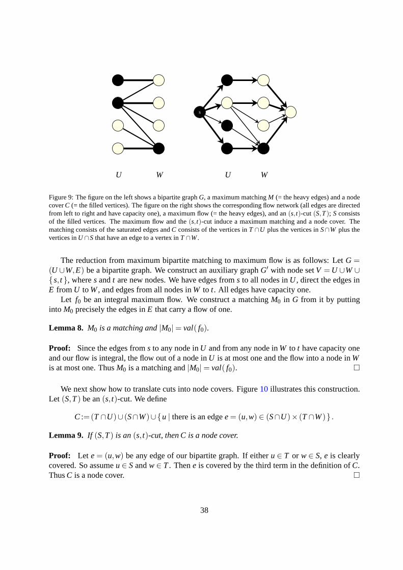
s

UU WW

Figure 9: The figure on the left shows a bipartite graphG, a maximum matchingM (= the heavy edges) and a nodecoverC (= the filled vertices). The figure on the right shows the corresponding flow network (all edges are directedfrom left to right and have capacity one), a maximum flow (= theheavy edges), and an(s,t)-cut (S,T); Sconsistsof the filled vertices. The maximum flow and the(s,t)-cut induce a maximum matching and a node cover. Thematching consists of the saturated edges andC consists of the vertices inT ∩U plus the vertices inS∩W plus thevertices inU ∩S that have an edge to a vertex inT ∩W.

The reduction from maximum bipartite matching to maximum flow is as follows: LetG =(U ∪W,E) be a bipartite graph. We construct an auxiliary graphG′ with node setV = U ∪W∪s, t , wheres andt are new nodes. We have edges froms to all nodes inU , direct the edges inE from U toW, and edges from all nodes inW to t. All edges have capacity one.

Let f0 be an integral maximum flow. We construct a matchingM0 in G from it by puttinginto M0 precisely the edges inE that carry a flow of one.

Lemma 8. M0 is a matching and|M0|= val( f0).

Proof: Since the edges froms to any node inU and from any node inW to t have capacity oneand our flow is integral, the flow out of a node inU is at most one and the flow into a node inWis at most one. ThusM0 is a matching and|M0|= val( f0).

We next show how to translate cuts into node covers. Figure10 illustrates this construction.Let (S,T) be an(s, t)-cut. We define

C :=(T ∩U)∪ (S∩W)∪u | there is an edgee= (u,w) ∈ (S∩U)× (T∩W) .

Lemma 9. If (S,T) is an(s, t)-cut, then C is a node cover.

Proof: Let e= (u,w) be any edge of our bipartite graph. If eitheru∈ T or w∈ S, e is clearlycovered. So assumeu∈ Sandw∈ T. Thene is covered by the third term in the definition ofC.ThusC is a node cover.

38

S

T

U W

...

......

...

Figure 10: The figure demonstrates how to obtain a node cover from a cut(S,T). The cover contains the nodesin T ∩U , S∩W and the source nodes of the edges in(S∩U)× (T ∩W). Every edge has an endpoint in a shadedregion, which shows that the set of vertices in the shaded region is a node cover.

Lemma 10. Let (S0,T0) be an(s, t)-cut with val( f0) = cap(S0,T0) and let M0 and C0 be thecorresponding matching and node cover. Then|M0|= |C0|.

Proof: We have

|M0|= val( f0)

= cap(S0,T0)

= |S0∩W|+ |T0∩U |+ |e= (u,w) ∈ (S0∩U)× (T0∩W)|≤ |S0∩W|+ |T0∩U |+ |u | there is an edgee= (u,w) ∈ (U ∩S0)× (W∩T0)|= |C0|,

where the second equality follows from the fact that there are |S0∩W| edges(w, t) in S0×T0

and |T0∩U | edges(s,u) in S0×T0 and the inequality follows from the fact that all edges inS0× T0 are saturated and hence counting endpoints inU is equivalent to counting the edgesin (S0∩U)× (T0∩W).

The example demonstrates how to design a certifying algorithm via a reduction to a differ-ent problem, for which a certifying algorithm is already known. After we describe the generalapproach to reductions, we explain why and how the previous example is a special case.

39

8.1.2. The General ApproachWe now describe a general approach for obtaining certifyingalgorithms via reductions.

Theorem 8. Let (ϕ,ψ) and (ϕ ′,ψ ′) be I/O-specifications and letW and W ′ be correspond-ing (strong) witness predicates. Let A′ be a (strongly, weakly) certifying algorithm for I/O-specification(ϕ ′,ψ ′) and witness predicateW ′. The translations f: X→ X′, g : X×Y′ → Y,h : X×Y′×W′→W transform inputs, outputs, and witnesses respectively. Assume further

W′( f (x),y′,w′) =⇒ W (x,g(x,y′),h(x,y′,w′)). (8)

If A′ is weakly certifying, also assume

ϕ(x) =⇒ ϕ( f (x)).

Then the following algorithm A is a (strongly, weakly) certifying algorithm for I/O-specification(ϕ,ψ) and witness predicateW .

1. translate x into f(x)

2. run A′ on f(x) to obtain y′ and w′

3. translate y′ into y= g(x,y′) and w′ into w= h(x,y′,w′) and return(y,w).

Proof: Assume first thatW andW ′ are (strong) witness predicates andA′ is a (strongly) cer-tifying algorithm. Letx ∈ X be arbitrary and letx′ = f (x) be the corresponding input forA′.Algorithm A′ terminates onx′ and returns a pair(y′,w′) with W ′(x,y′,w′). ThenW (x,y,w)by implication (8). ThusA is a (strongly) certifying algorithm for I/O-specification(ϕ,ψ) andwitness predicateW .

We come to the case thatA′ is weakly certifying. Letx ∈ X satisfyϕ(x). Thenϕ ′(x′) andhenceA′ terminates and returns a pair(y′,w′). ThusA terminates andW (x,y,w).

It may seem strange that the implicationϕ(x) =⇒ ϕ( f (x)) is only needed in the case ofweakly certifying algorithms. Note however, that even in this case, it is only used to concludethatA′ terminates onx′. Since (strongly) certifying algorithms are total, their termination is givenfor free. So assume thatf translates an inputx with ϕ(x) into anx′ with ¬ϕ ′(x′) andA′ producesa witnessw′ that proves thatx′ violates the precondition. In such a situation, it is unlikely that onecan prove the implicationW ′( f (x),y′,w′) =⇒ W (x,g(x,y′),h(x,y′,w′)). It is not impossible,e.g., if the I/O-specification(ϕ,ψ) is trivial.

Let us illustrate Theorem8 on our previous example. We have

• X = the set of all bipartite graphsG.

• X′ = the set of all directed networksG′ with designated nodessandt.

• f translates a bipartite graphG = (U ∪W,E) into a directed network.

40

• Y = the set of matchings inG (alternativelyY = all subsets ofE).

• Y′ = the set of integral(s, t)-flows in G′.

• ψ ′(G′, f ′) = T iff f ′ is a maximum flow inG′.

• ψ(G,M) = T iff M is a maximum matching inG.

• W′ = the set of(s, t)-cuts.

• W = the set of node covers inG.

• W ′(G′, f ′,(S′,T′)) = T iff val( f ′) = cap(S′,T ′).

• W (G,M,C) = T iff |M|= |C|.

• g translates an integral flow into a matching.

• Lemma8 proves thatg does as required.

• h translates an(S,T)-cut into a cover.

• Lemma9 shows thath does as desired.

• Lemma10 proves implication (8).

This shows that the example of the reduction from maximum cardinality bipartite matchingto maximum flow is indeed a special case of the general scheme of reductions.

8.2. Linear Programming Duality

Linear programming duality is a general technique for certifying algorithms. Linear pro-gramming is about optimizing linear objective functions inthe presence of linear constraints.The dual of a linear program can provide a witness of optimality.

For n nonnegative real variablesx = (x1, . . . ,xn), the goal is to maximize the linear functioncTx= ∑1≤ j≤nc jx j subject tom linear constraints. Thei-th constraint has the form∑1≤ j≤nAi j x j ≤bi . In matrix notation, a linear program is defined by anm×n real matrixA and real vectorscandb of dimensionn andm, respectively. The goal is to solve:

maxcTx subject to Ax≤ b andx≥ 0.

The dual linear program is a linear program inm nonnegative variablesy = (y1, . . . ,ym). Thereis one variable for each constraint of the primal linear program. The objective function to beminimized isyTb= ∑1≤i≤myibi. There is one constraint for each variable of the primal. Thej-thconstraint is∑1≤i≤myiAi j ≤ ci . Thus, in matrix notation the dual program can be formulatedas:

minyTb subject to yTA≥ cT andy≥ 0.

Lemma 11 (Linear Programming Duality). For linear programs, the following holds:

41

(a) Weak Duality: If x∗ and y∗ are solutions to a linear program and its dual, respectively, thencTx∗ ≤ y∗Tb.

(b) Complementary Slackness: Assume x∗ and y∗ are solutions to a linear program and its dual,respectively, with cTx∗ = y∗Tb. Let A(·,i) be the i-th column of A and let A( j ,·) be the j-th row

of A. Then ci = y∗TA(·,i) whenever x∗i > 0 and bj = A( j ,·)x∗ whenever yj > 0.

(c) Strong Duality: If both programs are feasible, then there are solutions x∗ and y∗ with cTx∗ =y∗Tb.

Proof: We only prove weak duality and complementary slackness. Forstrong duality, we referthe reader to any textbook on linear programming, e.g., [Sch86]. Weak duality is easy to prove.We have

cTx∗ ≤ y∗TAx∗ ≤ y∗Tb .

The first inequality follows fromcT ≤ y∗TA andx∗ ≥ 0 and the second inequality follows fromAx∗ ≤ b andy∗ ≥ 0.

Assume now thatcTx∗ = y∗Tb. Then both inequalities in the equation above must be equali-ties, i.e.,

cTx∗ = y∗TAx∗ = y∗Tb .

In particular for anyi with x∗i > 0, we must haveci = y∗TA(·,i) and for anyj with y∗j > 0, we musthaveb j = A( j ,·)x

∗, showing the complementary slackness.

So a certifying algorithm for solving linear programs outputs a primal solutionx∗ and a dualsolutiony∗ with cTx∗ = y∗Tb. Observe, that it is trivial to check whetherx∗ is a solution for theprimal, thaty∗ is a feasible solution for the dual, and thatcTx∗ = y∗Tb. Also the proof that thiscertifies optimality is trivial as we have seen above. It is only the existence ofx∗ andy∗ (i.e., thestrong duality) which is hard to prove, but this is not neededto be convinced.

The previous section, that deals with the reduction of bipartite matching to the computationof a maximum flow, shows an example of linear programming duality. The dual problem tothe maximum flow problem is the minimum(s, t)-cut problem. As a second example we nowconsider the minimum spanning tree problem.

Minimum Spanning Trees:.LetG=(V,E) be an undirected connected graph and letw : E→R≥0

be a nonnegative weight function on the edges. The goal is to find a spanning treeT ⊆ E ofminimum weightw(T) = ∑e∈T w(e).

What constitutes a proof of optimality? Figure11 illustrates such a proof; the drawing andthe usage of the word “moat” is inspired by [JP93]. For a partitionπ of the vertex set let #(π)be the number of blocks ofπ and letδ (π) be the set of edges whose endpoints belong to distinctblocks ofπ . Assume we have nonnegative valuesyπ , one for each partitionπ of the vertex set

42

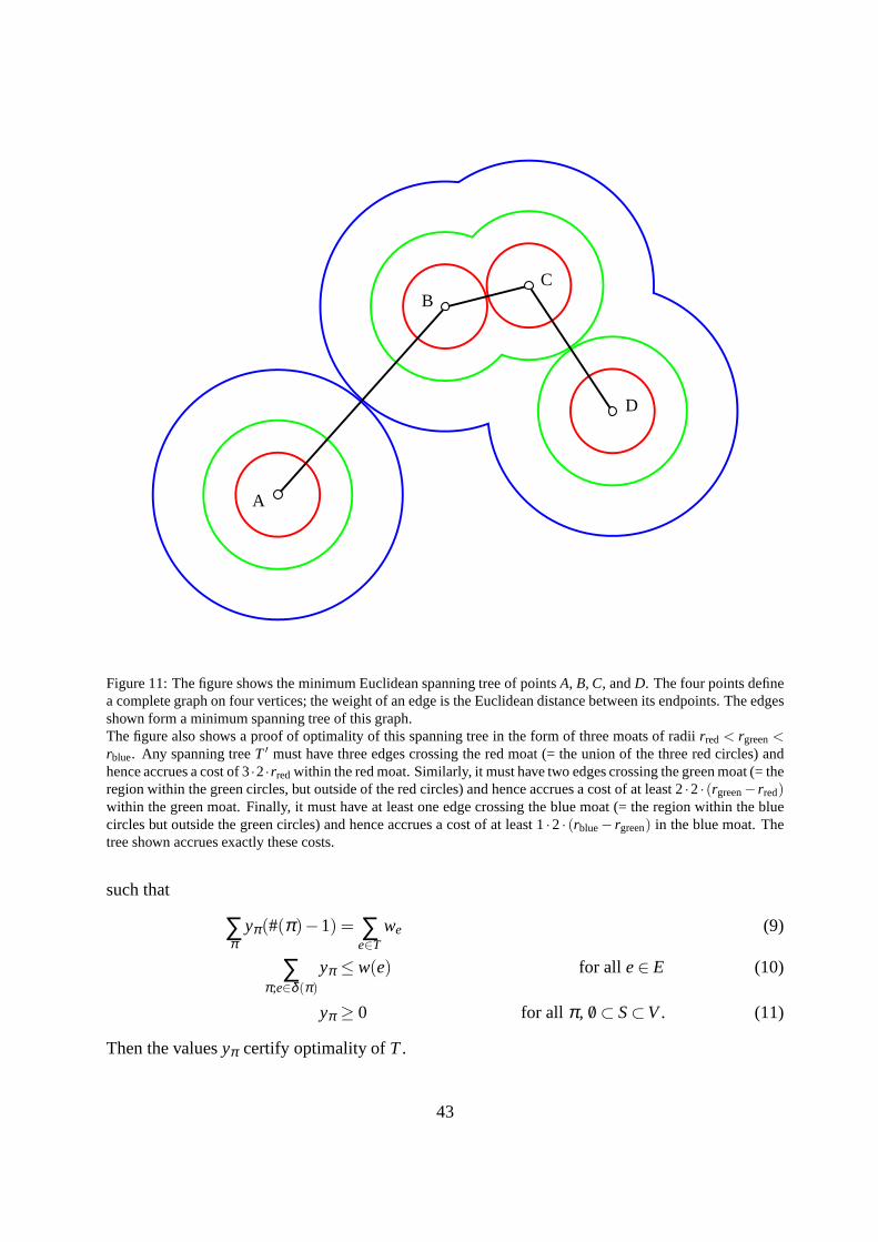
A

BC

D

Figure 11: The figure shows the minimum Euclidean spanning tree of pointsA, B, C, andD. The four points definea complete graph on four vertices; the weight of an edge is theEuclidean distance between its endpoints. The edgesshown form a minimum spanning tree of this graph.The figure also shows a proof of optimality of this spanning tree in the form of three moats of radiirred < rgreen<rblue. Any spanning treeT ′ must have three edges crossing the red moat (= the union of thethree red circles) andhence accrues a cost of 3·2·rredwithin the red moat. Similarly, it must have two edges crossing the green moat (= theregion within the green circles, but outside of the red circles) and hence accrues a cost of at least 2·2· (rgreen− rred)within the green moat. Finally, it must have at least one edgecrossing the blue moat (= the region within the bluecircles but outside the green circles) and hence accrues a cost of at least 1·2 · (rblue− rgreen) in the blue moat. Thetree shown accrues exactly these costs.

such that

∑π

yπ(#(π)−1) = ∑e∈T

we (9)

∑π;e∈δ (π)

yπ ≤ w(e) for all e∈ E (10)

yπ ≥ 0 for all π , /0⊂ S⊂V. (11)

Then the valuesyπ certify optimality ofT.

43

Lemma 12. If (9) to (11) hold, T is a minimum weight spanning tree.

Proof: Let T ′ be any spanning tree. For any partitionπ , the number of edges inδ (π)∩T ′ mustbe at least #(π)−1 and hence

w(T ′) = ∑e∈T ′

w(e) definition ofw(T ′)

≥ ∑e∈T ′

∑π;e∈δ (π)

yπ by inequality (10)

= ∑π

∑e∈T ′∩δ (π)

yπ change of order of summation

≥∑π

yπ(#(π)−1) since|T ′∩δ (π)| ≥ #(π)−1 andyπ ≥ 0

= w(T) by equation (9)

ThusT is a minimum spanning tree.

We next show how to compute the valuesyπ ; the construction will associate nonzero valuesyπ only with n−1 partitions. LetT be an alleged minimum spanning tree and lete1, e2, . . . ,en−1

be the edges ofT in increasing order of weight; ties are broken arbitrarily.Let π1 be the partitionconsisting ofn singleton blocks and, fori ≥ 2, letπi+1 be obtained fromπi by uniting the blockscontaining the endpoints ofei . Observe that the endpoints must be in distinct blocks sinceT is atree. We defineyπ = 0 for anyπ that is not inπ1, . . . ,πn−1. For simplicity, writeyi instead ofyπi and define6

yi =

we1 if i = 1

wei −wei−1 if i > 1.

Lemma 13. (9) to (11) hold for the values yπ as defined above.

Proof: All values yπ are nonnegative. The blocks ofπi are exactly the connected compo-nents of the graph(V,e1, . . . ,ei−1). Thusei has its endpoints in different blocks for all parti-tionsπ1,π2, . . . ,πi and has both endpoints in the same block ofπ j for j > i and hence

w(ei) = ∑2≤ j≤i

(w(ej)−w(ej−1))+w(e1) = ∑j≤i

yi = ∑π ; e∈δ (π)

yπ .

Consider next a non-tree edgee and leti be maximal such that the endpoints ofe are in distinctblocks ofπi. Thenemust connect the same blocks ofπi asei does; otherwise the endpoints ofewould be in distinct blocks ofπi+1. Thuse andei lie on a common cycle of(V,e1, . . . ,ei ,e)and hencew(e)≥ w(ei). Thus (10) holds.

6The radii of the moats shown in Figure11are half of theseyi ’s.

44

Finally, inspecting the proof of Lemma12 with T ′ = T, all inequalities must be equalitiesand hence (9) holds.

How does one arrive at this certificate? Linear Programming is the key ([CCPS98]). Thefractional minimum weight spanning subgraph problem is easily formulated as a linear program.We have a nonnegative variablexe for each edge. The value ofxe designates the fraction withwhich e belongs to the spanning subgraph. The goal is to minimize∑e∈E wexe. We have aconstraint for each partitionπ of V, namely that∑e∈δπ xe≥ #(π)−1, i.e., for each partition, wemust pick at least #(π)−1 edges connecting vertices in different blocks of the partition. We maydo so by picking edges fractionally. We obtain the followingformulation as a linear program.

minimize ∑e

wexe

subject to ∑e∈δ (π)

xe≥ #(π)−1 for all partitionsπ of V

xe≥ 0 for all e∈ E.

It is not obvious that this linear program always has an integral optimal solution. The dual linearprogram has a variableyπ for every partitionπ and reads:

maximize ∑π

(#(π)−1)yπ

subject to ∑π ; e∈δ (π)

yπ ≤ we for every edgee

yπ ≥ 0 for all π .

A spanning tree is an integral solution to the primal and Lemma 13 shows that there is a dualsolution with the same objective value. Thus a minimum spanning tree is an optimal solution tothe primal and the dual solution proves its optimality. Lemma 12 is a proof of weak duality forthis special case.

Verifying Linear Programs:.Linear programming duality is a great method for checking opti-mality of solutions to linear programs. Given a feasible solutionx∗ to the primal program linearprogram

maximizecTx subject toAx≤ b andx≥ 0

and a feasible solutiony∗ to the corresponding dual linear program

minimizeyTb subject toyTA≥ cT andy≥ 0

the equalitycTx∗ = y∗Tb (12)

implies optimality of both solutions. Unfortunately, linear programming solvers [CPL, SoP] forgeneral linear programs are numerical procedures and yieldonly approximate solutions. So we

45

AB xB

xN

yB yNbB

bN

cB cN

Figure 12: The decomposition into basic and non-basic variables. For simplicity, we assumed thatAB is the leftupper corner of the constraint matrix.

cannot hope that the computed approximate solutions satisfy equation (12). Fortunately, linearprogramming solvers also return a combinatorial description of the optimal solution in terms ofa basis.

A basis is a square non-singular sub-matrixAB of the constraint matrixA. We call the primalvariables corresponding to columns ofAB basic and denote them byxB; the other primal variablesare called non-basic and denoted byxN. Similarly, we call the dual variables corresponding torows ofAB basic and denote them byyB; the other dual variables are called non-basic and denotedbyyN. Analogously, we splitb intobB andbN andc intocB andcN, see Figure12. A basis inducesa primal solution(xT

B, xTN) (not necessarily feasible) and a dual solution(yT

B, yTN) (not necessarily

feasible) by way of:

ABxB = bB or xB = A−1B bB and xN = 0 (13)

yTBAB = cT

B or yTB = cT

BA−1B and yN = 0 (14)

The objective value of these solutions is equal. Indeed,

(cTB,cT

N)

(

xB

xN

)

= cTBxB = cT

BA−1B bB = yBbB = (yT

B, yTN)

(

bB

bN

)

.

A basis is primal feasible if ˆxB≥ 0 and is dual feasible if ˆyB≥ 0.

Lemma 14. If a basis is primal and dual feasible, the corresponding primal (xTB, xT

N) and dualsolution(yT

B, yTN) are optimal.

Proof: (xTB, xT

N) is a solution to the primal linear program,(yTB, yT

N) is a solution to the dual linearprogram, and their objective values are equal. Thus, the solutions are optimal by Theorem11.

Optimality of a basisB can now be checked as follows [DFK+03]. Equations (13) and (14)are used to compute the primal and dual solutions corresponding to the basis; the computationis carried out in exact rational arithmetic. If both solutions are feasible, the basis is optimal. Inthis way, the speed of floating point arithmetic is used to findthe optimal basis and the exactnessof rational arithmetic is used to certify the solution. If the basis is not optimal but “close tooptimal”, it can be taken as the starting basis for an exact primal or dual Simplex algorithm.The use of exact rational arithmetic can be replaced by the use of high-precision floating pointarithmetic [ACDE07].

46

8.3. Characterization Theorems

Within characterization theorems sometimes lies the potential to certify an output. We havealready seen examples of this: A graph is not planar if and only if it contains a Kuratowskisubgraph (see Section2.6), and a graph is not 3-connected if and only if it contains a separatingpair (see Section5.4).

Interestingly these characterizations follow a certain pattern: One direction of the proof ofthe characterization is easy, and this side corresponds to required simplicity of the witness. Themore difficult direction is the one required to establish theexistence of a witness.

To clarify this statement we provide another example: A graph G is perfectif the chromaticnumber of every induced subgraphH of G is equal to the size of the largest clique ofH.

An odd holein a graph is an induced odd cycle of length at least 5, anodd anti-holeisan induced subgraph isomorphic to the complement of an odd hole. The strong perfect graphtheorem [CRST06] says that a graph is perfect if and only if it contains neither an odd hole noran odd anti-hole.

The chromatic number of odd holes and of odd anti-holes is notequal to the size of theirlargest clique, so they cannot be contained in a perfect graph. This easy part of the characteriza-tion shows that odd holes and odd anti-holes certify a graph to be not perfect. The second part ofthe strong perfect graph theorem, the existence of an odd hole or an odd anti-hole in a non-perfectgraph, resolves a conjecture that had been open for more than40 years. The polynomial-timealgorithm for the recognition of perfect graphs [CCL+05] detects an odd hole or an odd anti-holein a perfect graph, and thereby certifies a graph to be not perfect.

8.4. Approximation Algorithms and Problem Relaxation

Approximation algorithms compute nearly-optimal solutions of optimization problems. Theycome with a guarantee for the quality of approximation. We may assume w.l.o.g. that we dealwith a minimization problem. In the proof of correctness thequality of the solution is usuallymeasured against an easy to compute lower bound for the problem. A certifying approximationalgorithm should output (in a certifying way) a lower bound in addition to the solution. This caneither be the lower bound used in the proof of correctness or another lower bound. The generaltechnique for obtaining lower bounds is problem relaxation, i.e., enlarging the set of feasiblesolutions. We give an example.

The traveling salesman problem asks for a shortest cycle visiting all vertices of a edge-weighted undirected graphG = (V,E,c). The costc(C) of a cycleC is the sum of the costsof the edges contained inC. We assume thatc satisfies the triangle inequality, i.e,c(uv) ≤c(uw)+c(wv) for any triple of verticesu, v andw. There are approximation algorithms whichproduce a solution whose cost is at most 1.5 times the optimum[LLRKS85]. We discuss twolower bounds for the traveling salesman problem: 1-trees and the subtour elimination linearprogram. Both approaches yield the same value, but use very different principles [CCPS98].

Lower Bounds via 1-Trees.A 1-tree anchored at a vertex v[HK70] is a spanning tree ofG\ vplus two edges incident tov. A 1-treeis a 1-tree anchored at some vertexv of G. As for cycles,the cost of a 1-tree is the sum of the costs of the edges in the 1-tree. A minimum 1-tree is a1-tree of minimum cost. Minimum 1-trees are readily computed by n minimum spanning tree

47

computations since the minimum 1-tree anchored at a vertexv is simply a minimum spanningtree ofG\v plus the two cheapest edges incident tov.

Minimum 1-trees can be used to lower bound the cost of any traveling salesman tour. Forthis letπ be any real-valued function defined on the vertices ofG and consider the modified costfunctioncπ(uv) = c(uv)+π(u)+π(v). We callπ a potential function. The cost of a one-treeTunder the cost functioncπ is defined ascπ(T) = ∑uv∈T cπ(uv). Accordingly, a minimum 1-treewith respect to the modified costπ is a 1-tree with minimal modified cost.

Lemma 15. Let C be a traveling salesman tour, letπ be a potential function, and let T be aminimum 1-tree with respect toπ . Then

cπ(T)−2 ∑v∈V

π(v)≤ c(C).

Proof: Sincec satisfies the triangle inequality, there is a tourD visiting every vertex exactlyonce and having cost no more thanC. This tourD is a 1-tree (with respect to any anchor) andhence

cπ(T)≤ cπ(D).

SinceD uses exactly two edges incident to any vertex,

c(D) = cπ(D)−2 ∑v∈V

π(v).

Combining the equalities and inequalities, we obtain

c(C)≥ c(D) = cπ(D)−2 ∑v∈V

π(v)≥ cπ(T)−2 ∑v∈V

π(v).

A certifying approximation algorithm for the traveling salesman problem outputs a tourC, apotential functionπ and a minimum 1-treeT for cπ , and a proof of optimality ofT. The proofof optimality reduces to the minimum spanning tree problem,for which we have discussed acertifying algorithm in Subsection8.2.

A good potential functionπ can be found by an iterative process ([HK70, HK71]). Observethat

cπ(T)−2 ∑v∈V

π(v) = c(T)+ ∑v∈V

degT(v)π(v)−2 ∑v∈V

π(v) = c(T)+ ∑v∈V

(degT(v)−2)π(v),

where degT(v) is the number of edges ofT incident tov. We conclude that the vector(degT(v)−2)v∈V is the gradient of the expressioncπ(T)−2∑v∈V π(v) viewed as function ofπ .

We start an iterative process withπ(v) = 0 for all v. In an iteration, we first compute theminimum 1-treeT with respect to the current modified cost functioncπ . If T is a tour, i.e.,degT(v) = 2 for all v, we stop;T is an optimal tour. Otherwise, we updateπ to π ′ as follows:

π ′(v) = π(v)+ ε(degT(v)−2) for all v∈V,

48

whereε > 0 is a small value; this is a small step in the direction of the gradient and increases thepotential value of vertices of degree three or higher and decreases the potential value of verticesof degree one.7 We setπ = π ′ and repeat. The iterative process produces a sequence of lowerbounds. We remember the best lower bound computed in this wayand use it to produce a lowerbound for our problem, as described above.

Lower Bounds via Linear Programming.An integer linear programming formulation of the trav-eling salesman problem is as follows. We have a decision variablexe for each edge of the graphwith the intention that the edges withxe = 1 comprise an optimal solution. A tour contains twoedges incident to every vertex and for every non-empty proper subsetS of V there must be atleast two edges in any tour with exactly one endpoint inS. We obtain the following formulationas an integer linear program.

minimize ∑e

cexe

subject to ∑e∈δ (v)

xe = 2 for all v∈V

∑e∈δ (S)

xe≥ 2 for all Swith /0 6= S 6= V

xe∈ 0,1 for all e∈ E

Here we useδ (S) to the denote the set of edges with exactly one endpoint inS. The equalityconstraint for vertexv is called adegree constraintand the inequality for subsetS is called asubtour elimination constraint. Consider any solution of this system and letT be the edgespicked; e∈ T iff xe = 1. ThenT contains two edges incident to every vertex and hence is acollection of cycles. Assume for the sake of a contradiction, that the collection consists of morethan one cycle and letSbe the vertex set of one of the cycles. ThenT contains no edge inδ (S)and hence violates the subtour elimination constraint forS.

The subtour LP is obtained from the ILP by replacing the constraintxe∈ 0,1 by the weakerlinear constraint 0≤ xe≤1. Thus the subtour LP is a relaxation of the traveling salesman problemand provides a lower bound. Figure13gives an example. In this example, the cost of an optimumtour is 10 and the objective value of the subtour LP is 9. The gap may be as large as a factor oftwo [CCPS98].

The subtour LP has an exponential number of constraints, onefor each non-empty proper sub-set of the vertices. It can be solved in polynomial time by means of the ellipsoid method [Sch03].

7For an edgeuv, we havecπ ′(uv) = cπ(uv)+ ε(degT(u)+degT(v)−4). Also,

cπ ′(T)−2 ∑v∈V

π ′(v) = cπ(T)−2 ∑v∈V

π(v)+ ε ∑v∈V

(degT(v)−2)2.

Thus the cost of the 1-treeT increases by the change of the potential function. However,at π ′ a different 1-treemay be minimal and hence it is not guaranteed that the iteration produces better and better lower bounds. In fact, ingeneral, it does not do so.

49

2

1

22

1

2

2

1

2

1/2

1

1/21/2

1

1/2

1/2

1

1/2

Figure 13: The figure on the left shows the edge costs; there are six edges of cost two and three edges of cost one.The figure on the right shows an optimal solution to the subtour LP. The decision variables corresponding to theedges of cost two have value 1/2 and the decision variables corresponding to the edges of cost one have value 1. Thesolution has cost 9. The optimal tour has cost 10.

In practice, one uses the simplex method and a judiciously chosen subset of the subtour elimina-tion constraints. The subset is determined dynamically by atechnique calledseparation. Let (x∗e)be a solution to an LP comprising the degree constraints, thebounding constraints 0≤ xe≤ 1,and some of the subtour elimination constraints. Consider an auxiliary graph with vertex setV,edge setE, and set the capacity of the edgee to x∗e. Then(x∗e) violates a subtour eliminationconstraint if and only if this auxiliary graph has a cut of capacity less than two. Such a cut canbe found by a minimum cut computation [SW97]. If a violated subtour elimination constraint isfound, it is added to the LP, and the LP is resolved.

In Section8.2we learned how to verify solutions to linear programs. Now wewant to certifya lower bound and this can be done by a simple rounding procedure [ABC+09]. Consider thedual for the subtour LP. It has an unconstrained variableπv for each vertexv, a non-negativevariableyS for each non-empty proper subsetS of V, and a non-negative variableze for eachedgee. The variableze corresponds to the upper bound constraintxe≤ 1. The goal is to

maximize 2∑v

πv +2∑S

yS−∑e

ze

subject to πu+πv + ∑S;e∈δ (S)

yS−ze≤ ce for e= (u,v) ∈ E

yS≥ 0 for all Swith /0 6= S 6= V

ze≥ 0 for all e

50

If the primal or dual LP is solved by an LP-solver, the basis returned is not necessarily optimal.Also, primal feasibility and dual feasibility are not guaranteed. However, the solutions are usu-ally close to optimal. In the case of the subtour LP, this can be exploited as follows. Consider any(not necessarily feasible) dual solution(πv), (yS), and(ze). We first replace any negativeyS byzero and we then choose theze large enough so that all dual constraints are satisfied. In this way,we obtain a feasible dual solution and hence a lower bound forthe traveling salesman problem.

8.5. Composition of Programs

Suppose that we have certifying algorithms for I/O-behaviors (ϕ1,ψ1) and (ϕ2,ψ2). Howcan we obtain a certifying algorithm for the composed behavior? That’s easy.

Let Q1 andQ2 be certifying algorithms for the two I/O-behaviors, respectively, and letC1 andC2 be the corresponding checkers. A certifying algorithm for the composed I/O-behavior worksas follows: Assume that our input isx.

RunQ1 onx. This producesy and a witnessw1.if (y =⊥) then

Output⊥ and the witness(w1,⊥,⊥)else

RunQ2 ony. This produceszand a witnessw2.Outputz and the witnessw = (w1,y,w2).

end ifThe checkerC for the composed behavior accepts(w′,y,w′′) as a witness if

y =⊥ and C1 accepts(x,y,w′) or (15)

C1 accepts(x,y,w′) and C2 accepts(y,z,w′′). (16)

Two I/O-behaviors should only be composed if the postcondition of the first behavior impliesthe precondition of the second behavior, i.e.,ψ1(x,y) =⇒ ϕ2(y). If Q2 is strongly certifying, itcan discover a misuse of composition: Assume that they output byQ1 does not satisfyϕ2. ThenQ2 will either produce az with ψ2(y,z) and a proof that it did so or a proof for¬ϕ2(y). In theformer case,Q2 could handley although it did not have to do so, in the latter caseQ2 states thatits precondition is violated.

9. Further Examples

In the introductory Section1 we have discussed the examples of bipartition, connected com-ponents, shortest paths, greatest common divisors, maximum cardinality matchings and pla-narity. In Subsection5.2 we discussed a strongly certifying algorithm that five-colors a planargraph and in Subsection5.4 we described a simple way to certify triconnectedness. We nowdiscuss further illustrative examples, demonstrating thebroad applicability of certification.

9.1. Convexity of Higher-dimensional Polyhedra and ConvexHulls

The convex hull of a finite setSof points ind-dimensional space is the smallest convex setcontainingS. Its boundary is a piecewise linear hyper-surface. There are many algorithms for

51

higher-dimensional convex hulls [CK70, PS85, Sei86, CS89, CMS93] and implementations ofsome [BDH96, MMN+98, CGA]. In 2 and 3 dimensions the output of a geometric algorithm canbe visualized and this helps debugging geometric programs.In higher dimensions, visualizationis not possible. How can one certify the output of a convex hull algorithm?

What is the output? All algorithms output the boundary of theconvex hull as a simplicialpiecewise linear hypersurfaceF . We will define this term below. In 3-dimensional space theboundary is given as a set of triangles (in 3-space) that are glued together at their edges.

Task 1. Given a set S of points and a hyper-surfaceF verify thatF is the boundary of theconvex hull of S.

We split this task into two subtasks.

Subtask 1. Given a piecewise linear simplicial hyper-surfaceF in d-dimensional space verifythatF is the surface of a convex polytope.

Assume thatF is the surface of a convex polytope and letP be the convex polytope whoseboundary isF .

Subtask 2. Verify that

• every vertex of P is a point in S and that

• every point of S is contained in P.

We discuss the two subtasks in turn. This section is based on [MNS+99, Section 2.3]. Analternative solution can be found in [DLPT98]. We first deal with the Subtask1, whether a simpli-cial piecewise linear hyper-surfaceF without boundary ind-dimensional space is the boundaryof a convex polytope. We assume that the hyper-surface is given by its facet graph. The facetgraph is ad-regular graph whose nodes are labeled byd-tuples of affinely independent points,i.e., each node corresponds to an oriented(d−1) simplex (= a facet of the surface). The hyper-plane supporting a facet dividesd-space into a positive and a negative halfspace. Neighboringnodes differ in their labeling by exactly one point and for everyone of thed vertices of a facetthere must be such a neighboring facet. In other words, edgescorrespond to(d−2)-simplicesshared by two facets. Neighboring nodes must be labeled consistently, i.e., the negative halfspacecorresponding to adjacent facets must agree locally.

Let us interpret this definition in 3-space. Every node of thefacet graph corresponds to anoriented triangle in 3-space. Oriented means that the two sides of the triangle are distinguished,one is “outside” and one is “inside” (in the paragraph above,inside and outside are called negativeand positive, respectively). Adjacent triangles share twovertices and differ in one. Every trianglehas three neighbors and the two sides of adjacent triangles are locally consistent.

For smooth surfaces, already Hadamard described a test for convexity.

Theorem 9 (Hadamard). Let F be a smooth compact surface inRd without boundary and let

d > 2. If F is locally convex at everyone of its points thenF is the surface of a convex body.

52

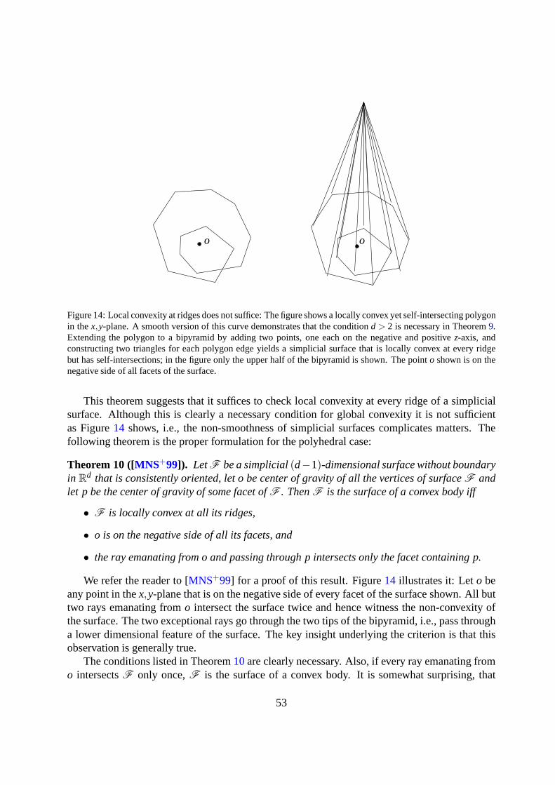
o o

Figure 14: Local convexity at ridges does not suffice: The figure shows a locally convex yet self-intersecting polygonin thex,y-plane. A smooth version of this curve demonstrates that theconditiond > 2 is necessary in Theorem9.Extending the polygon to a bipyramid by adding two points, one each on the negative and positivez-axis, andconstructing two triangles for each polygon edge yields a simplicial surface that is locally convex at every ridgebut has self-intersections; in the figure only the upper halfof the bipyramid is shown. The pointo shown is on thenegative side of all facets of the surface.

This theorem suggests that it suffices to check local convexity at every ridge of a simplicialsurface. Although this is clearly a necessary condition forglobal convexity it is not sufficientas Figure14 shows, i.e., the non-smoothness of simplicial surfaces complicates matters. Thefollowing theorem is the proper formulation for the polyhedral case:

Theorem 10 ([MNS+99]). LetF be a simplicial(d−1)-dimensional surface without boundaryin R

d that is consistently oriented, let o be center of gravity of all the vertices of surfaceF andlet p be the center of gravity of some facet ofF . ThenF is the surface of a convex body iff

• F is locally convex at all its ridges,

• o is on the negative side of all its facets, and

• the ray emanating from o and passing through p intersects only the facet containing p.

We refer the reader to [MNS+99] for a proof of this result. Figure14 illustrates it: Leto beany point in thex,y-plane that is on the negative side of every facet of the surface shown. All buttwo rays emanating fromo intersect the surface twice and hence witness the non-convexity ofthe surface. The two exceptional rays go through the two tipsof the bipyramid, i.e., pass througha lower dimensional feature of the surface. The key insight underlying the criterion is that thisobservation is generally true.

The conditions listed in Theorem10are clearly necessary. Also, if every ray emanating fromo intersectsF only once,F is the surface of a convex body. It is somewhat surprising, that

53

it suffices to compute the number of intersections for a single ray. The verification is easy toprogram.

• Check local convexity at every ridge. If local convexity does not hold at some ridge declareF non-convex.

• Seto to the center of gravity of the vertices ofF and check whethero is on the negativeside of all facets. If not, declareF non-convex.

• Choose any facet and letp be the center of gravity of its vertices. Letr be the ray emanatingfrom o and passing throughp. If r intersects the closure of any other facet ofF declareF non-convex.

• If F passes all three tests declare it the surface of a convex polytope.

We next turn to the Subtask2. Assume thatF passed the convexity test and letP be theconvex polyhedron with boundaryF . We need to verify that

• every vertex ofP is a point inSand that

• every point ofS is contained inP.

The first item is fairly easy to check. If the vertices ofP are equipped with pointers toelements inS, the check is trivial. If the vertices ofP are specified by their coordinate tuples, thecheck involves a dictionary lookup.

The second condition is much harder to check. In fact, without additional information (= thewitness), there seems to be no efficient way to verify it. A simple method would be to checkevery point ofSagainst every facet ofF . However, the complexity of this method is an order ofmagnitude larger that the complexity of the most efficient convex hull programs8. An alternativemethod is to use linear programming to check that all non-vertices are non-extreme9. For fixeddimension the alternative method is quadratic in the numberof vertices. For variable dimensionone might hope that a simplex-based verification procedure has good expected running time.Nevertheless, both approaches essentially resolve the original problem. We conclude that convexhull programs that output the hull as a convex polytope are hard to check. The “gift-wrapping”algorithm [CK70] falls in this category.

What is an appropriate witness that makes checking easy? Here is one. Arrange the points inS in a linear order and for each pointp in S that is not a vertex ofP indicate a set ofd+1 pointsthat come later in the ordering and that containp in their convex hull. We call such an orderinganadmissible orderingof S.

8Algorithms based on randomized incremental construction [CS89, CMS93, BMh94] run in time related to thesize of the output and the size of intermediate hulls and the algorithm of [Sei86] is guaranteed to construct the hullin logarithmic time per face.

9The linear program hasd variables corresponding to the coefficients of a linear function. For each vertex ofFthere is a constraint stating that the function value at the vertex is negative. For each non-vertex consider the linearprogram that maximizes the function value at this point.

54

Lemma 16. An admissible ordering of S proves that every point of S is contained in P.

Proof: Let q1 to qn be an admissible ordering ofS. We show that eachqi is a convex combina-tion of vertices ofP. We use induction oni starting atn and going down to 1. Consider anyi. Ifqi is a vertex ofP, there is nothing to show. Otherwise,qi is a convex combination of points thatcome later in the ordering. By induction hypothesis, these points are convex combinations of thevertices ofP. Thusqi is a convex combination of the vertices ofP.

The witness is easily checked. For each point that is claimedto be a convex combination ofpoints later in the ordering, one needs to solve a linear system.

The algorithms based on randomized incremental construction [CS89, CMS93, BDH96,MMN+98, CGA] can be modified to compute this witness. They compute a simplicial com-plex10 comprising the hull, i.e., a set of simplices whose union isP. They do so incrementally.They start withd + 1 points ofS spanning a simplex and then add point after point. If a newpoint p is contained in the current hull, they determine a simplex inthe current simplicial com-plex containingp. The vertices of this simplex are the witnesses forp. If the new pointp isoutside the current hull, they determine all facets of the current hull visible from the new point.For each such facetF they add a simplexS(F, p) with baseF and tipp to the simplicial complex.

Assume now that the algorithm is rerun: first the vertices ofP are inserted (in random order)and then the non-vertices (in any order). In this way, all simplices in the simplicial complex havetheir vertices among the vertices inP and each non-vertex inS is placed in a simplex spanned byvertices ofP.

9.2. Solving Linear Systems of Equations

We consider a systemAx = b of m linear equations inn unknownsx; hereA is a m by nmatrix of real numbers andb is anm-vector. We want to know whether there is a solution tothis system. Again, a conventional algorithm would just return a single bit, telling whether thesystem is solvable or not.

A certifying algorithm would do a lot more. If it declares thesystem solvable, it would returna solution, i.e., ann-vectorx0 such thatAx0 = b. Observe that it is very easy to verify whether agivenx0 is a solution. We simply plugx0 into the equation.

If it declares the system non-solvable, it could return anm-vectorc such thatcTA = 0 andcTb 6= 0. Observe that such a vector witnesses non-solvability. Indeed, assume the existence of asolutionx0. ThencTAx0 = (cTA)x0 = 0Tx0 = 0 andcTAx0 = cT(Ax0) = cTb 6= 0, a contradiction.Thus there is no solution.

Why does such ac exist? IfAx= b has no solution,b does not belong to the space spanned bythe columns ofA. Thus we can writeb asb= b′+b′′, whereb′ is in the span of the columns ofAandb′′ is orthogonal to all columns ofA. We can takec= b′′. ThencTA= 0 andcTb= b′′Tb′′ 6= 0.

How can we compute such ac? We use Gaussian elimination. It is well known that it returnsa solution when given a solvable system. It is less well knownthat it also returns a witness

10A simplicial complex is a set of simplices the intersection of any two is a face of both.

55

for non-solvability when given an unsolvable system. We describe Gaussian elimination as arecursive procedure. If all entries ofA andb are zero, the zero-vector 0n is a solution. If allentries ofA are zero andb is nonzero, saybi 6= 0, them-vectorei having a one in positioni andzero everywhere else witnesses non-solvability.

So assume thatA has a nonzero entry, sayAi j 6= 0. We subtract a suitable multiple of thei-thequation from all other equations (i.e., we subtractAl j /Ai j times thei-th equation from thel -thequation for 1≤ l ≤m and l 6= i) so as to eliminate thej-th variable from the other equations.The transformation yields a system withm−1 equations inn−1 unknowns, sayA′x′ = b′. HereA′lk = Alk−(Al j /Ai j )Aik andb′l = bl−(Al j /Ai j )bi for l 6= i and allk. Also, row indexi and columnindex j are deleted from the index set of the reduced system. Assume first that the reduced systemis solvable andx′0 is a solution. We plugx′0 into thei-th original equation, solve forx j and obtaina solution to the original system. Assume next that the reduced system is unsolvable and thatc′ witnesses it, i.e.,c′TA = 0 andc′Tb′ 6= 0. We define them-vectorc by cl = c′l for l 6= i andci =−∑l 6=i(Al j /Ai j )c′l . Then for anyk, 1≤ k≤ n,

∑l

cl Alk = ciAik +∑l 6=i

cl Alk

= ciAik +∑l 6=i

c′l (A′lk +(Al j /Ai j )Aik)

= (ci +∑l 6=i

c′l (Al j /Ai j ))Aik +∑l 6=i

c′l A′lk

= ∑l 6=i

c′l A′lk

= 0 .

An analogous computation shows thatcTb = c′Tb′ and hencecTb 6= 0. We have now shown thatGaussian elimination easily turns into a certifying solverfor linear systems of equations.

9.3. NP-Complete Problems

Branch-and-Bound and Brunch-and-Cut are powerful methodsfor computing optimal so-lutions to NP-complete problems [ABCC06]. The algorithms use a heuristic for computing afeasible solution and compute a matching lower bound (we again assume a minimization prob-lem) for the objective value of any feasible solution to prove optimality. For the latter, theypartition the search space and compute a lower bound for eachcell of the partition. The heuristicsolution is optimal if its objective value matches the lowerbound.

In the case of the Traveling Salesman Problem (see Subsection 8.4) the partition is usually byinclusion and exclusion of edges. For example, we might divide the search space into two parts,by considering all tours containing a particular edgeuv and all tours not containing this edge.Figure15shows an example. The two cells obtained in this way can be subdivided further usingthe same strategy recursively. In each cell a lower bound is computed, e.g., using the methods ofsubsection8.4. In summary, the approach is as follows.

• Use a heuristic to find the optimum solution. Verify that the solution is feasible.

56

0 1

2

3

4

5

2, x0,1 = 12

1

2

1

22

2

1

0 1

2

3

4

5

2 2

1

22

2

1 1

0 1

2

3

4

5

11/2

1/2

1/2

1

1/21/2

1

1/2

Figure 15: In the example of Figure13, the optimal solution to the subtour LP is fractional;x0,1 has value 1/2. Wegenerate two subproblems. In the first subproblem, we setx0,1 to 1 and force the edge into the tour. In the secondsubproblem, we setx0,1 to 0; this is tantamount to deleting the edge. For both subproblems, the subtour LP (in fact,the LP with only the degree constraints) has objective value10. For the first subproblem there is a non-integralsolution of value 10 as shown on the right, there is also an integral solution of value 10.

• Partition the space of feasible solutions. Verify that the partition is indeed a partition.

• Compute for each cell of the partition a lower bound on the objective value of the feasiblesolutions in this cell. Verify that the lower bound computedfor each cell is indeed a lowerbound and has at least a value equal to the cost of the heuristic solution computed in thefirst step.

The first two steps are typically simple. For the last step, one uses the techniques discussed inSection8.4. In [ABC+09], Applegate et. al. report about the the certification of an optimal TSPtour through 85,900 cities. The tour was obtained by a heuristic [Hel06] and then verified by theapproach outlined above.

As a second example consider the satisfiability problem of propositional logic. Letϕ be aboolean formula. A satisfying assignment is a witness of satisfiability. A resolution proof is awitness of non-satisfiability. The resolution proof may have exponential length; it is however,easy to check.

9.4. Maximum Weight Independent Sets in Interval Graphs

Given a collection of weighted intervals, the goal is to find an independent set of maximumweight. We usei to denote a generic interval andI to denote an independent set. The goal is thento find an independent setI of intervals of maximal weight∑i∈I wi , wherewi > 0 is the weightof interval i. This problem is one of the introductory examples in the textbook of Kleinberg andTardos [KT05].

The standard algorithm for this problem uses dynamic programming. Assume that the inter-vals are numbered in the order of their left endpoint. The optimal solution either contains interval1 or it does not. Thus

Opt(1,n) = max(Opt(2,n),w1+Opt( j,n))

57

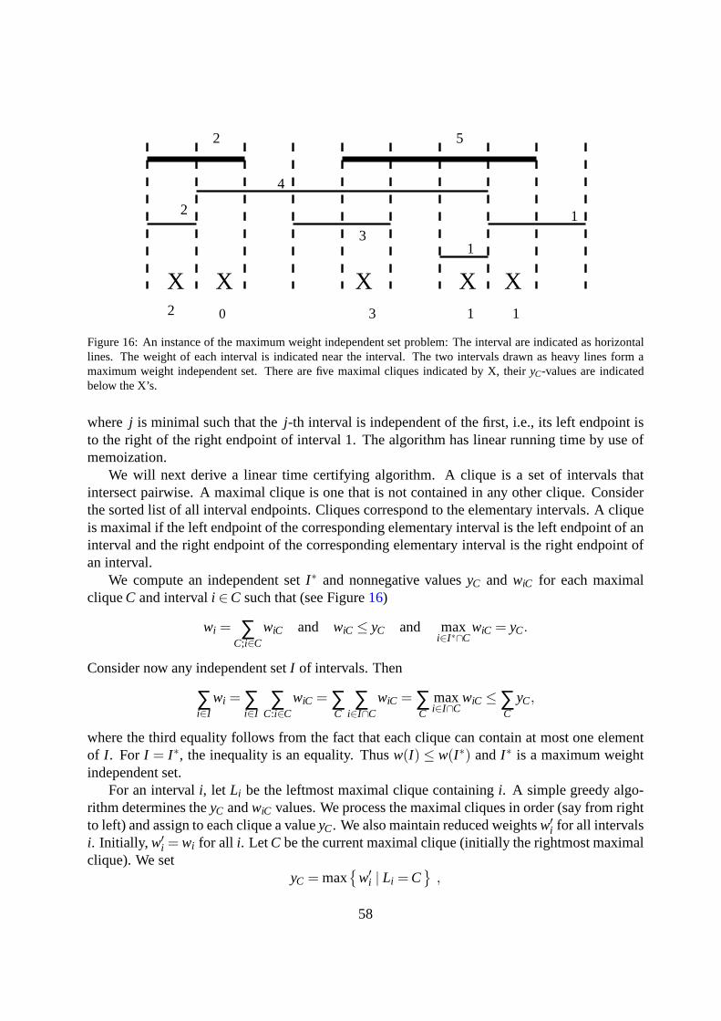
0

X X X X X1 1

1

1

2

2

2

3

3

4

5

Figure 16: An instance of the maximum weight independent setproblem: The interval are indicated as horizontallines. The weight of each interval is indicated near the interval. The two intervals drawn as heavy lines form amaximum weight independent set. There are five maximal cliques indicated by X, theiryC-values are indicatedbelow the X’s.

where j is minimal such that thej-th interval is independent of the first, i.e., its left endpoint isto the right of the right endpoint of interval 1. The algorithm has linear running time by use ofmemoization.

We will next derive a linear time certifying algorithm. A clique is a set of intervals thatintersect pairwise. A maximal clique is one that is not contained in any other clique. Considerthe sorted list of all interval endpoints. Cliques correspond to the elementary intervals. A cliqueis maximal if the left endpoint of the corresponding elementary interval is the left endpoint of aninterval and the right endpoint of the corresponding elementary interval is the right endpoint ofan interval.

We compute an independent setI ∗ and nonnegative valuesyC and wiC for each maximalcliqueC and intervali ∈C such that (see Figure16)

wi = ∑C;i∈C

wiC and wiC ≤ yC and maxi∈I∗∩C

wiC = yC.

Consider now any independent setI of intervals. Then

∑i∈I

wi = ∑i∈I

∑C:i∈C

wiC = ∑C

∑i∈I∩C

wiC = ∑C

maxi∈I∩C

wiC ≤∑C

yC,

where the third equality follows from the fact that each clique can contain at most one elementof I . For I = I ∗, the inequality is an equality. Thusw(I) ≤ w(I ∗) andI ∗ is a maximum weightindependent set.

For an intervali, let Li be the leftmost maximal clique containingi. A simple greedy algo-rithm determines theyC andwiC values. We process the maximal cliques in order (say from rightto left) and assign to each clique a valueyC. We also maintain reduced weightsw′i for all intervalsi. Initially, w′i = wi for all i. LetC be the current maximal clique (initially the rightmost maximalclique). We set

yC = max

w′i | Li = C

,

58

i.e., we setyC to the maximal reduced weight of any interval havingC as its leftmost maximalclique. Maximality ofC guarantees that there is at least one such interval. Also, for any icontained inC, we setwiC to the minimum ofyC andw′i and reducew′i by wiC.

An interval i is calleddefiningfor C if C = Li andyC = wiC andyC > 0. A cliqueC withyC = 0 has no defining interval. An interval is called tight forC if wiC = yC. The followingLemma is key (and also obvious).

Lemma 17. If i is defining for Li then i is tight for all cliques containing it.

Proof: If i is defining forLi , wiL i = yLi > 0. This implieswiC = yC for all maximal cliquescontainingi.

We next construct the independent setI ∗. LetC be the leftmost clique. If its valueyC is zero,we move on to the next clique. Otherwise, leti be defining forC. We addi to I ∗ and remove allcliques containingi and all intervals intersecting with it from the problem. Observe that, by thepreceding Lemma,wiD = yD for all cliquesD removed and that the intervals removed have theirleftmost maximal clique among the removed cliques. In otherwords, the remaining cliques keeptheir defining intervals. We continue with the leftmost remaining clique. In this way, we havefor everyC with positiveyC an intervali in I ∗ with wiC = yC.

9.5. String Matching

Given a text stringT0T1 . . .Tn−1 and a patternP0 . . .Pm−1, the string matching problem is todecide whether the pattern occurs in the text string, i.e., whether there is a positioni such thatTi+ j = Pj for 0≤ j < m. In such a situation, we say that the pattern occurs with shift i.

For the purpose of certification, if the pattern is found the position is output. A certificate forthe contrary case may be given in the form of an arrayw that indicates for each shift a specificcharacter mismatch. The arrayw that satisfiesw[i] = min j | Ti+ j 6= Pj provides exactly that:placing the pattern into the text with a shift ofi creates a mismatch at positioni +w[i]. To verifythe validity of the certificate it suffices to checkw[i] ∈ 0, . . .m−1 andTi+w[i] 6= Pw[i] for alli ∈ 0, . . . ,n−m.

We now show how the Knuth-Morris-Pratt algorithm can be modified to provide such a cer-tificate with its answer. Surprisingly, we could not find thismodification in the literature. As iscustomary, we extend the pattern by a character $ that does not match any other character, i.e.Pm = $ andTi 6= $ 6= Pj for 0≤ i < n and 0≤ j < m. Assume for the time being that we have atour disposal a functionw′, where

w′(i) = min

j | Pi+ j 6= Pj

for 1≤ i ≤m. It will be computed along with the prefix functionπ , where

π(q) = max(−1∪

h | h < q andP0 . . .Ph = Pq−h . . .Pq

).

The functionsw′ andπ are related. For allq and allℓ with 1≤ ℓ < q−π(q) we haveℓ+w′(ℓ)≤ q.Indeed,P0 . . .Pπ(q) matchesPq−π(q) . . .Pq andπ(q) is maximal with this property. Thus if we

59

T0 T1 . . . Tt . . . Tt+q−π(q)−1 Tt+q−π(q) . . . Tt+q Tt+q+1

= . . . = = . . . = 6=P0 . . . Pq−π(q)−1 Pq−π(q) . . . Pq Pq+1

= . . . =P0 . . . Pπ(q)

Figure 17: A typical situation during string matching.

placeP at positionℓ of P with 1≤ ℓ < q−π(q), we must have a mismatch before positionq.Thusℓ+w′(ℓ)≤ q.

Assume now the longest prefix of the pattern that matches the substring of the text startingfrom positiont is of lengthq, see Figure17. We claim that in this situation we can easilycompute the valuesw(t + ℓ) for ℓ ∈ 0,1, . . . ,q−π(q)−1. First we observe thatw(t) = q+1by definition. Forℓ ∈ 1, . . . ,q− π(q)− 1 we claimw(t + ℓ) = w′(ℓ). Indeed aligningP atpositiont + ℓ of the text is the same as aligning it at positionℓ of the pattern, at least for the nextq+ 1 characters. The mismatch withP occurs at positionℓ+ w′(ℓ) and since this number is atmostq, the mismatch withT occurs att + ℓ+w′(ℓ). Thusw(t + ℓ) = w′(ℓ).

Similar to the computation of theπ function, the computation ofw′ can be done by employingthe same algorithm to match the pattern against itself. Recursive calls tow′ values will onlyinvoke positions that are smaller and have already been computed.

In the analysis of the running time we would see that for everypositioni there is exactly oneassignment forw(i) whose right hand side involves only a number or a previously knownw value.The corresponding statement forw′ holds equally, therefore the total running time increases byat mostO(m+n).

9.6. Chordal Graphs

A chordon a simple cycle is an edgeuv that is not an edge of the cycle but whose endpointsare vertices on the cycle. A graph ischordal if every simple cycle of length at least four has achord. The ability to efficiently recognize chordal graphs played a key role in linear time algo-rithms for recognizing interval graphs, which are chordal,and is discussed at length in [Gol80]and the introductory textbook [KT05].

To certify that a graph is not chordal, it suffices to point outa chordless cycle. The checkermust check that this cycle is, indeed, a cycle of the graph, and it must check that this cycle ischordless. This can be done by marking the vertices and then cycling through the edges to makesure that no edge that is not part of the cycle has two marked endpoints.

The certificate that a graphG is chordal is similar to the topological sort as a certificatethata graph is a directed acyclic graph. If(v1,v2, . . . ,vn) is an ordering of the vertices ofG, thenthe rightward neighborsof vi are those neighbors ofvi that lie to its right in the ordering. Theordering is aperfect elimination orderingif the rightward neighbors of everyvi induce a completesubgraph.

A graph is chordal if and only if it has a perfect elimination ordering. Thus, an eliminationorder can serve as a witness that a graph is is chordal.

60

Algorithm 1 KMP-MATCHER1: n← length[T]; m← length[P]2: π ← COMPUTE-PREFIX-FUNCTION(P)3: q←−14: for i =−1 ton−2 do5: // We haveT[i−q] . . .T[i] = P[0] . . .P[q] andi−q plays the role oft in Figure176: while q≥ 0 andP[q+1] 6= T[i +1] do7: w(i−q)← q+18: for ℓ = 1 toq−π(q)−1 do9: w(i−q+ ℓ)← w′(ℓ)

10: end for11: q← π[q]12: end while // eitherq =−1 orP[q+1] = T[i +1]13: if P[q+1] = T[i +1] then14: q← q+115: else16: w(i)← 017: end if // T[i +1−q] . . .T[i +1] = P[0] . . .P[q]18: if q = m−1 then19: print “Pattern occurs with shifti−m”20: end if21: end for

Algorithm 2 COMPUTE-PREFIX-FUNCTION1: m← length[P]2: π[0]←−1; q←−13: for i = 0 to m−1 do // We haveπ[i] = q and henceP[i−q] . . .P[i] = P[0] . . .P[q]4: while q≥ 0 andP[q+1] 6= P[i +1] do5: w′(i−q)← q+16: for ℓ = 1 toq−π(q)−1 do7: w′(i−q+ ℓ)←w′(ℓ)8: end for9: q← π[q]

10: end while // eitherq =−1 orP[q+1] = P[i +1]11: if P[q+1] = P[i +1] then12: q← q+113: else14: w′(i)← 015: end if // P[i +1−q] . . .P[i +1] = P[0] . . .P[q]16: π(i +1) = q17: end for

61

To understand why, letG be a graph that is not chordal, and suppose(v1,v2, . . . ,vn) is aperfect elimination ordering. SinceG is not chordal, it has a chordless cycleC of size at leastfour. Letvi be the leftmost vertex ofC in the ordering. Then its neighborsv j andvk onC lie toits right, and sinceC has no chord,v j andvk are non-adjacent, contradicting the assumption that(v1,v2, . . . ,vn) is a perfect elimination ordering.

It is harder to prove that every chordal graph has a perfect elimination ordering, but thisimplication is not needed to be convicted that the input graph is chordal.

A linear-time algorithm to find a perfect elimination ordering is given in [RTL76]. Theobvious checker for the perfect elimination order takes longer to run than it takes to produce thewitness. It must check that for each vertexvi , the rightward neighbors ofvi form a completesubgraph, which takes time that is quadratic in the number ofthese neighbors. Over allvi , asingle edge can be checked many times.

In [RTL76] an algorithm is given that checks the witness inO(n+ m) time. The trick is topostpone the checks in such a way that each edge is checked only once.

The algorithm traverses the perfect elimination ordering(v1,v2, . . . ,vn). Inductively,vi hasreceived a listA(vi) of vertices from its predecessors(v1,v2, . . . ,vi−1). The algorithm ensures thatvi is adjacent to these vertices, or else declares the witness as invalid. If it passes this test, it thendetermines the leftmost rightward neighborv j of vi and appends the other rightward neighborsof vi to A(v j).

For the correctness, if(v1,v2, . . . ,vn) is not a perfect elimination ordering, then somevi hasrightward neighborsv j andvk that are non-adjacent. Suppose without loss of generality thatj < k. It is easily seen by induction fromi to j that if the algorithm has not rejected the orderingby the time thatA(v j) is checked, thenvk is in A(v j). The algorithm will therefore reject thewitness when it discovers thatA(v j) contains a non-neighbor ofv j .

The algorithm can be implemented to run inO(n+m) time using elementary methods, suchas marking the neighbors ofvi before checkingA(vi), and then unmarking them before movingon tovi+1.

The algorithm originally proposed for determining whethera graph is chordal included analgorithm that produces a perfect elimination ordering if agraph is chordal, and an imperfectelimination ordering if it is not [RTL76]. The paper therefore included the above algorithm forchecking whether an ordering is a perfect elimination ordering. It did not describe how to finda chordless cycle if the input graph is not chordal. The paperwas then followed by a shortaddendum explaining how to do this [TY85].

9.7. Numerical Algorithms

Numerical algorithms are usually implemented in floating point arithmetic. As floating pointarithmetic incurs round-off error, numerical computations do not always yield good approxima-tions of the true result. Almost every textbook in numericalanalysis contains warning examples.The field of validated numerical computations [Her94, Rum01] addresses this issue and devel-ops methods that deliver rigorous results. It is beyond the scope of this paper to elaborate onvalidated numerical computations and so we confine ourselves with a simple example.

Let a be a positive real number. We have some method for computing square roots, say the

62

method returnsx0. How good isx0? The following estimate is useful:

|√

a−x0|=a−x2

0√a+x0

≤

a−x20

1+x0if a≥ 1

a−x20

a+x0if a < 1

As a concrete example, let us estimate the distance of√

2.5 and 1.58. We have

|√

2.5−1.58| ≤ 2.5−2.49641+1.58

=0.00362.58

≤ 0.0015.

9.8. Guide to Literature

Frequently, algorithms research that is performed with efficiency in mind leads implicitlyto methods suitable to certify the output. For various algorithmic problems however, specificalgorithms that allow for certification had to be and have been designed. We briefly survey someexamples.

Graph recognition problems:.For various graph classes certified recognition algorithmsex-ist. Among these classes are the interval and permutation graphs [KMMS06], the circular andunit circular arc graphs [KN06], the proper Helly circular arc graphs [LSS07], the HHD-freegraphs [NP07], and the co-graphs [LdR07] (for which there is also a dynamic version [CP06]).Proper interval graphs are treated in [Mei05] and [HH05], the latter also considers bipartite per-mutation graphs. Further certified recognition algorithmsfor several hereditary graph classes aregiven in [HK07].

Connectivity and two-connectivity are easily certified in linear time. A spanning tree certi-fies connectivity, a cut vertex certifies non-two-connectivity, and every s-t-numbering, open eardecomposition and bipolar orientation certifies two-connectivity [Bra02]. For triconnectednessof graphs, linear decision algorithms are known [HT73, MR92]. The fastest certifying algorithmruns in quadratic time (See Subsection5.4 and [Sch10]). A linear-time certifying algorithmfor graphs for which a Hamiltonian cycle is known is available [EMS10]; this assumes that theHamiltonian cycle is part of the input. For arbitraryk, the situation is as follows. In lineartime anyk-connected graph can be sparsified to ak-connected graph withO(kn) edges [NI92].Of course, certifyingk-connectivity of the sparsification certifiesk-connectivity of the originalgraph. Also, it is easy to check whether a vertex cut in the sparsification is also a vertex cut in theoriginal graph.k-connectivity can be tested in timeO(m+min(kn2,k2n3/2)) ([Eve75, Gal80]);the algorithms are certifying. The certificates are flows. [LLW88] gave a geometric charac-terization ofk-connectivity for generalk. A graphG is k-connected if and only if, specifyingany k vertices ofG, the vertices ofG can be represented as points inR

k−1 so that nok are ona hyperplane and each vertex is in the convex hull of its neighbors, except for thek specifiedvertices. The characterization gives rise to anO(n5/2 + nk5/2) time Monte Carlo algorithm fork-connectivity and anO(kn5/2 +nk7/2) Las Vegas algorithm fork-connectivity. The algorithmsare certifying.

63

Permutation groups:.In [CMPS03] certifying algorithms for computational problems involvingpermutation groups given by generators are considered. More specifically, the problems consid-ered are deciding membership, subgroups, computing orbits, the Schreier tree, stabilizers, bases,and computing the order of the given permutation group.

Geometric Problems:.In [Ber05] a certifying algorithm for minimally rigid planar graphs isgiven. The papers [DLPT98] and [MNS+99] describe methods for certifying convexity of poly-hedra and convex hulls (see Subsection9.1) and various types of planar subdivisions, such astriangulations, Delaunay triangulations, and convex subdivisions. Another application of localto global principles for certification of convexity can be found in [Ryb09].

Miscellaneous:.[FK00] shows how to certify a large hidden clique in a semi-random graph and[McC04] explains how to certify whether a matrix has the consecutive ones property. Certifica-tion of various basic graph algorithms (with and without witnesses) are discussed in [Met97].

Implementations:.Implementations of many certifying algorithms and the corresponding check-ers are discussed in [MN99]. For the algorithm library LEDA the concept of certification hasbeen and is one of the guiding principles.

10. Randomization

In the preceding sections, we considered deterministic certifying algorithms and determin-istic checkers. In this section we consider randomization.We first explain that deterministiccheckers turn Monte Carlo algorithms into Las Vegas algorithms. We then give three examplesof randomized certification. The first two examples have a checker that does not require a wit-ness. In the third example the provided witness allows for a faster running time of the randomizedchecker. Finally, we extend Section5 to randomized algorithms.

10.1. Monte Carlo Algorithms resist Deterministic Certification

Consider a Monte Carlo algorithm for a functionf , i.e., a randomized algorithm which on in-putx outputsf (x) with probability at least 3/4 and may output anything otherwise. The runningtime is bounded byT(|x|).

Assume now that there were an efficient certifying algorithmQ with the same complexity: oninput x algorithmQ outputs a triple(x,y,w) passing the witness predicateW with probability atleast 3/4 and may output anything else otherwise. It has running timeO(T(|x|)). Further assumethere is a deterministic checkerC that checks the triple(x,y,w) in time O(T(|x|)). We can turnQ into a Las Vegas algorithm forf as follows: We first runQ. If the triple(x,y,w) returned byQpassesW , we returny. Otherwise, we rerunQ.

The resulting randomized algorithm always returns the correct result f (x) and has an ex-pected running time inO(T(|x|)). Observe that each round has an expected running time inO(T(|x|)) since both the algorithmQ and the checkerC run within this time. Also observe thatthe expected number of rounds is constant, since the successprobability is at least 3/4.

Does this observation imply that Monte Carlo algorithms areinherently unsafe? No, it onlysays that the concept of deterministic certification does not apply to them. Program verification

64

does apply and Monte Carlo algorithms are frequently quite simple so that verification maybe(come) feasible. Another option is to deviate from the deterministic checkers by allowingrandomization and error. We describe three examples in the next three subsections. The first twoexamples demonstrate use of randomized certification without the help of a witness, whereasthe third example makes use of a witness to provide randomized certification of the output of arandomized algorithm.

10.2. Integer Arithmetic

To check the result of a multiplication computation, the following method used to be taughtin German high-schools and is already described by Al-Kharizmi in his book on algebra. It isknown as “Neunerprobe” in German, “casting out nines” in English, and “preuve par neuf” inFrench.

We want to check whetherc= a·b. We form the repeated digit sumssa, sb andsc of a, b andc. The digit sum is formed by adding the digits of a number. If the result is a multi-digit number,the process is repeated, until one arrives at a one digit number. For example,

4572→ 18→ 9.

Then one multipliessa andsb with a two-digit result; lets be the digit sum of the the result. Ifs 6= sc, thenc is not equal toa ·b. If s= sc, thenc may or may not be equal toa ·b.

The digit sum of a positive integera is nothing but the remainder ofa modulo 9 (with repre-sentatives 1 to 9 instead of 0 to 8). This follows from 10k mod 9= 1 for all k≥ 1. Thus castingout nines rests on the statement

if c = a ·b thenc mod 9= ((a mod 9) · (b mod 9)) mod 9.

Of course, a similar statement holds for any integerq instead of 9, i.e.,

if c = a ·b thenc modq = ((a modq) · (b modq)) modq.

Let sa = a modq and definesb andsc analogously. Lets= (sa ·sb) modq. If s 6= sc, thenc 6= a·b.If s= sc, q dividesc−a ·b. The number of distinct prime divisors ofc−a ·b is bounded. Thus,if we chooseq from a sufficiently large setP of primes, the test will showc 6= a ·b with highprobability. The following theorem quantifies these statements.

Theorem 11. Let a, b, and c be positive integers bounded by22k, with k≥ 5. If c 6= a ·b then

1. for any integer d> 0 the probability that a prime number x taken uniformly at randomfrom the primes within2, . . . ,2k+2d+3−1 divides c−a ·b is at most1/2d,

2. the probability that an integer x taken uniformly at random from1, . . . ,2k+5−1 does notdivide c−a ·b is at least1/(2 · (k+5) ln2), and

3. the probability that at least one of L= 2k+ 10 integers x1,x2, . . . ,xL taken uniformly atrandom from1, . . . ,2k+5−1 does not divide c−a ·b is at least1/2.

65

Proof: 1.) The absolute value ofc−ab is bounded by 22k+1+1. To show the statement, we will

show that there are sufficiently many prime numbers in the interval 2, . . . ,2k+3+2d−1, andthen, by bounding the number of prime factors of any number nolarger than 22

k+1+1, we willshow that most of these prime numbers are not prime factors of|c−ab|.

There are at least 2k+3+2d/((k+ 3+ 2d) ln2) prime numbers which are contained in theinterval2, . . . ,2k+3+2d−1. (This is in accordance with the prime number theorem that there areapproximatelyx/ ln(x) prime numbers smaller thanx and follows from Dusart’s bound [Dus98],since 2k+3+2d > 599). On the other hand for any integerx that hasℓ distinct prime factors, it mustbe the case thatℓ! ≤ n. It suffices for us to show that the number of primes in2, . . . ,2k+3+2d−1is by a factor of 2d larger than the number of distinct prime factors of|c−ab|. Thus it suffices toshow that

(

2k+3+2d

2d · (k+3+2d) ln2

)

! ≥ |c−ab|.

Since 2ln2< 2, for k≥ 1 it is true that

2k+3+2d ≥ (2k+1+1) ·22d · (2ln2),

thus2k+3+2d

22d ·2ln2≥ 2k+1+1.

By a simple expansion of the fraction it follows that

2k+3+2d

2d · (k+3+2d) ln2· (k+3+2d)

2d2≥ 2k+1+1 (17)

Sincek ≥ 1 andd ≥ 1, we have(k+ 3+ 2d)/(2d2) ≤ log(2k+3+2d/(2d · (k+ 3+ 2d)eln2)):Indeed, the inequality holds fork = 1 andd = 1. Furthermore, fork,d ∈R≥1, the partial deriva-tives with respect tok andd of the left side of the equation are smaller than the respective partialderivatives of the right side of the equation. We can thus replace the second factor on the left sideof Equation17and it follows that

2k+3+2d

2d · (k+3+2d) ln2· log

(

2k+3+2d

2d · (k+3+2d)eln2

)

≥ 2k+1 +1.

Stirling’s inequalityx! ≥ (x/e)x implies log(x!)≥ xlog(x/e), applying this we proceed to obtainthe desired inequality

(

2k+3+2d

2d · (k+3+2d) ln2

)

! ≥ 22k+1+1≥ |c−ab|.

2.) The second statement follows directly from the first by again noting that fork ≥ 11andd = 1 the number of primes in2, . . . ,2k+5−1 is at least 2k+5/((k+5) ln2).

3.) For anyi, 1≤ i ≤ L, the probability thatxi dividesc−ab is at most 1−1/(2(k+5) ln2)by the second statement. Therefore, the probability that all xi ’s dividec−ab is at most

(

1− 12(k+5) ln2

)L

= eL·ln

(

1− 12(k+5) ln2

)

≤ e− L

2(k+5) ln2 ≤ e− ln2 =12.

66

The asymptotic complexity of division is the same as the one of multiplication. Intuitively,multiplication is simpler than division. We can check a divisiona/b = c by checking whethera = c·b.

10.3. Matrix Operations

Given threen×nmatricesA, B, andC overZ2, we want to verify thatAB=C. There is an ob-vious way to check the equality: compute the product ofA andB and compare the result entry byentry withC. This takes timeO(nω), whereω is the exponent of matrix multiplication [CW82].

Already in 1977, R. Freiwalds [Fre77] described a randomized algorithm for verifying matrixmultiplication. The algorithm is simple. We generate a random vectorx ∈ Z

n2 and compute

y = A(Bx)−Cx. If y is the zero vector, we accept the input, i.e., believe thatC = AB, otherwisewe state thatC 6= AB. The computation ofy takes three matrix-vector products (Bx, A(Bx), andCx) and one vector addition and hence takes timeO(n2).

Let X = AB−C. Theny = Xx. If AB= C and henceX = 0, we havey = 0 for any choice ofx. If y 6= 0, thenX 6= 0 and henceAB 6= C. It remains to estimate the probability thatX 6= 0 andXx= 0.

Lemma 18 ([Fre77]). Let z be a nonzero n-vector overZ2. Then

prob(zTx 6= 0) = 1/2,

where x is a random n-vector overZ2.

Proof: Sincez is nonzero, there is anℓ with zℓ = 1. Then

zTx = xℓ + ∑j 6=ℓ

zjx j

and hence for any choice of thex j ’s, j 6= ℓ, there is a exactly one choice forxℓ such thatzTx 6= 0.

Theorem 12 ([Fre77]). Let X be a nonzero n×n matrix overZ2. Then

prob(Xx 6= 0)≥ 1/2

where x is a random n-vector overZ2.

Proof: SinceX is nonzero, it has at least one nonzero row. We apply the previous Lemma tothis row.

For further information on certification of matrix productssee [KS93]. We now turn to anexample that requires a witness to allow for the randomized certification.

67

2

1 3

4C1 C2 C3 C4

5

68

7

Figure 18: The leftmost figure shows a graph with eight edges.The next four figures show four circuits in thisgraph. The circuitC1 has the vector representationC1 = (0,1,1,1,1,1,0,0). Let D = (1,1,1,1,0,0,0,0) be thecircuit formed by the edges 1 to 4. ThenD = C1 +C2+C3 +C4. The setC1,C2,C3,C4 is a cycle basis. Its weightis equal to three times the sum of the weights of edges 1 to 4 plus 2 times the weight of edges 5 to 8.

10.4. Cycle Bases

We discuss the certification of minimum weight cycle bases ofundirected graphs. The fastestknown algorithm for computing a minimum weight basis is a Monte Carlo algorithm with run-ning timeO(mω), whereω is the exponent of matrix multiplication [AIJ+09]. The algorithm canbe made certifying and the witness can be checked in Monte Carlo timeO(m2). We describe therequired modifications and show how to check the witness. We refer the reader to [KLM +09] forbackground information on cycle bases.

Let G = (V,E) be a connected graph withn vertices andm edges and letw : E→ R>0 be apositive weight function on the edges ofG. All results of this section also hold for nonnegativeweight functions, but some of the arguments are shorter for positive weight functions. AcycleinG is an even subgraph ofG and acircuit is an even connected subgraph with all vertices havingdegree two, see Figure18. The weightw(C) of a cycle is the sum of the weights of its edges.We represent cycles as vectors inZ

E2 ; the coefficient corresponding to an edge is 1 if and only

if the edge belongs to the cycle. The space of all cycles is then a vector space of dimensionν = m−(n−1); observe that the addition of two cycles corresponds to the symmetric differenceof their edge sets and hence yields a cycle. A setB = C1, . . . ,Cν of cycles is a cycle basis ifany cycleC can be written as a linear combinationC = ∑i λiCi with λi ∈ Z2 for all i. Let T be aspanning tree ofG. For any non-tree edgee let Ce be the circuit formed bye plus the path inTconnecting the endpoints ofe. There arem−n+1 such cycles. They are independent and form abasis; this is called the fundamental cycle basis. The weight of a basis is the sum of the weightsof the cycles comprising the basis. A minimum weight basis isa basis of minimum weight.

The following lemma defines a certificate for minimum weight bases. For its proof, we firstobserve that every graph has a minimum cycle basis consisting only of circuits: Indeed, if thereis a cycleC in a basisB that is not a circuit, thenC is the union of two cyclesC′ andC′′ ofsmaller weight. ThenB−C+C′ andB−C+C′′ have smaller weight thanB and at least oneof them is a basis.

Lemma 19 ([dP95]). A set of cyclesC1, . . . ,Cν is a minimum cycle basis if there are vectors

68

S1,. . . ,Sν ∈ 0,1E such that11

(a) 〈Si,Cj〉= 0 for 1≤ i < j ≤ ν,

(b) 〈Si,Ci〉= 1,

(c) Ci is a shortest circuit with〈Si ,C〉= 1.

Proof: Let k be maximal such thatBk = C1, . . . ,Ck is contained in some minimum cyclebasis and assume, for the sake of a contradiction, thatk< ν. LetB′= C1, . . . ,Ck,Dk+1, . . . ,Dν be a minimum cycle basis extendingBk. Then

Ck+1 = ∑i≤k

λiCi + ∑i>k

λiDi (18)

and hence1 = 〈Sk+1,Ck+1〉= ∑

i>k

λi〈Sk+1,Di〉.

Thus there must be anℓ > k with λℓ = 〈Sk+1,Dℓ〉 = 1. By (c),w(Ck+1)≤ w(Dℓ). Solving (18)for Dℓ gives a representation ofDℓ in terms ofB′′ = B′ \Dℓ∪Ck+1. We conclude thatB′′

is a basis of weight no larger thanB′. Thus there is a minimum basis extendingBk+1.

We next describe a probabilistic check of conditions (a), (b), and (c) that operates in timeO(m2). The following observation will be useful.

Lemma 20 ([AIJ +09]). Let A1, . . . ,Ak,S∈ ZE2 . Then

〈Ai ,S〉= 1 for some i,1≤ i ≤ k =⇒ prob(〈 ∑1≤i≤k

λiAi ,S〉= 1) = 1/2,

where theλi , 1≤ i ≤ k, are chosen independently and uniformly inZ2.

Proof: Assume〈Aℓ,S〉= 1. Then for any choice of theλi, i 6= ℓ, there is exactly one choice forλℓ such that〈∑1≤i≤k λiAi ,S〉= 1, namelyλℓ = 1+ 〈∑i 6=ℓ λiAi ,S〉.

Alternatively, we observe that〈 ∑1≤i≤k

λiAi,S〉

is the inner product of a random vector(λ1, . . . ,λk) with the nonzero vector(〈A1,S〉, . . . ,〈Ak,S〉)and then appeal to Lemma18.

We first show how to verify properties (a) and (b). LetA be matrix whose rows are the vectorsST

1 to STν and letB be the matrix whose columns are the cyclesC1 to Cν . We need to verify that

11〈 , 〉 denotes the inner product of vectors.

69

E := AB is a lower-diagonal matrix with ones on the diagonal. Property (b) is easily verifiedin time O(νm) = O(m2). We simply compute the products〈Si,Ci〉 for 1≤ i ≤ ν. We turn toproperty (a). The solution lies in Lemma20. Consider the above-diagonal elements in thej-thcolumn, i.e., the elementsEi, j for i < j. One of these elements is nonzero if and only if one ofthe vectorsS1 to Sj−1 is non-orthogonal toCj . Lemma20 is a probabilistic test for this property.We choose random numbersλi ∈ Z2, 1≤ i ≤ n, and form the vectors

Rj = ∑i< j

λiSi , 1≤ j ≤ n.

These vectors can be computed in total timeO(nm). We next form the products

〈Rj ,Cj〉, 1≤ j < n.

If one of these products is nonzero,C is not a lower-diagonal matrix. Conversely, ifC is not alower-diagonal matrix, then with probability at least one-half, one of these products is nonzeroby Lemma20.

We next turn to condition (c). A circuitC is isometricif for any two verticesu andv in C, ashortest path connectingu andv is contained inC.

Lemma 21 ([Hor87]). A minimum cycle basisB consists only of isometric circuits.

Proof: We argue by contradiction. SupposeC is not an isometric cycle but contained in aminimum cycle basisB. Then there are verticesu andv in C such thatC does not contain ashortest path connectingu andv. Let p be a shortest path connectingu andv and splitC atu andv into C1 andC2. ConsiderC′ = C1 + p andC′′ = C2 + p. Both cycles are cheaper thanC andeitherB−C+C′ or B−C+C′′ is a basis.

The argument of the proof also shows that any cycle that fulfills condition (c) in Lemma19is an isometric circuit. To certify condition (c), we assumefor simplicity from now on that theshortest path between every two vertices of the input graph is unique; such a situation can besimulated by adding a random infinitesimally small weight toevery edge. For further detailssee [AIJ+09].

Lemma 22 ([AIJ +09]). Let C be an isometric circuit. Then for each v∈C there is an edge e=xy∈C such that C consists of the shortest paths from v to x and y andthe edge e.

Proof: Consider any edge ine= xyof C. SplittingC\eatv gives us a pathqv,x and a pathqv,y.There is a choice ofe (there might be two) such that both paths have weight at mostw(C)/2.SinceC is isometric, it contains a shortest path connectingv to x and a shortest path connectingv to y. These paths must beqv,x andqv,y, respectively.

We use the following witness for supporting the check of condition (c).

• For each vertexv, a shortest path treeTv rooted atv.

70

• A list L = (D1, . . . ,DN) of circuits that allegedly contains all isometric circuits. The circuitsare sorted by weight and the total size (= number of edges) of the circuits inL is at mostnm.

• For an edgee= xy and a vertexv letCv,e = pvx+e+ pvy, wherepvx is the path fromv to xin Tv. For eache andv, the algorithm provides a link to a circuitD ∈ L with D = Cv,e or aproof thatCv,e is non-isometric. The proof is a pair(a,b) of vertices onCv,e such that theshortest path connecting(a,b) is not part ofCv,e.

The algorithm in [AIJ+09] computes such a listL and the additional information stipulated above.Verification is as follows.

We first verify that the trees are shortest paths trees as described in Subsection2.4; we thenverify that all elements ofL are circuits, and that the total size of the circuits inL is nm. Wethen choose for each edgee a random labelℓ(e) ∈ Zp for a primep (p = 2 is sufficient) andprecompute for eachv and each nodex of Tv, the sum of the labels of the edges on the path fromv to x and for eachD in L the sum of the labels of the edges inD. This takes timeO(nm). Foreache= xy andv we perform the following test:

• If Cv,e is linked toD in L we compute the label ofCv,e (as the sum ofℓ(e) and the labelsof the endpoints ofe in Tv) and compare it to the label ofD. If the labels are different, wereject. The probability of failure to detectCv,e 6= D is bounded by 1/p.12 (This test wasproposed in [WC81] as a general method for verifying equality of sets.)

• If Cv,e is claimed to be non-isometric and(a,b) is provided as a proof we verify thata andb lie on the pathspv,x∪ pv,y wheree= xy; saya lies on the former path andb lies on thelatter. If a andb would lie on the same path, we reject, since subpaths of shortest pathsare shortest. We then compute the lengths of the two paths inCv,e connectinga andb (oneis w(pv,a)+ w(pv,b) and one isw(e)+ w(pa,x)+ w(pb,y)) and verify that these length arelarger thanw(pa,b). If not, we reject.

We have now verified thatL contains all isometric circuits. It remains to verify that thecircuits selected satisfy (c). LetL = D1, . . . ,DN and recall thatL is sorted in order of increasingweight. We choose a randomλ j ∈ 0,1 for each j and for eachℓ, 1≤ ℓ ≤ N form the sum∑ j≤ℓ λ jD j . For eachi, 1≤ i ≤ µ, letCi = Dπ(i). Verify

〈Ci ,Si〉= 1 and〈 ∑j<π(i)

λ jD j ,Si〉= 0.

By Lemma20, the latter test fails with probability 1/2 if there is aj < π(i) with 〈D j ,Si〉= 1.

Theorem 13. The witness for minimum cycle bases defined above can be checked in proba-bilistic time O(m2). The minimum cycle basis algorithm of [AIJ+09] can compute this witnesswithout loss of efficiency.

12 LetC andD be subsets ofE withC 6= D. Lete0∈C⊕D be an edge in the symmetric difference ofC andD. Thenfor each choice of labels of the edges inE \e, there is exactly one choice forℓ(e0) such that∑e∈C ℓ(e) = ∑e∈D ℓ(e).

71

10.5. Definitions

We extend the definitions and theorems of Section5 to randomized algorithms. Aprob-abilistically checkable strong witness predicatefor an I/O-specification(ϕ,ψ) is a predicateW : X×Y⊥×W satisfying the following properties:

Strong Witness Property: Let (x,y,w) ∈ X×Y⊥×W satisfy the witness predicate. Ify =⊥, wproves thatx does not satisfy the precondition and ify∈Y, w proves that(x,y) satisfies thepostcondition, i.e.,

∀x,y,w (y =⊥ ∧W (x,y,w)) =⇒ ¬ϕ(x) and(y∈Y∧W (x,y,w)) =⇒ ψ(x,y)

(19)

Randomized Checkability: For a triple(x,y,w) there is a trivial way to determine the valueW (x,y,w) with high probability. I.e., there is a trivial randomized algorithm that computesW (x,y,w) correctly with probability at least 3/4 and this bound on the error probability istrivial to understand.

Simplicity: The implications (19) have a simple proof.

The first and the last item are as in Section5. Observe that the checker is allowed to reject acorrect output and witness or accept a wrong output and witness with probability 1/4. The latteris important; otherwise the construction of Subsection10.1would apply.

A randomized strongly certifying algorithmfor I/O-specification(ϕ,ψ) and probabilisticallycheckable strong witness predicateW is an algorithm with the following properties:

• It halts for all inputsx∈ X.

• On inputx∈ X it outputs ay∈Y⊥ and aw∈W such thatW (x,y,w) holds with probabilityat least 7/8.

The simplicity and checkability consideration of Subsection5.5apply.The definition above captures all examples given in this section. We illustrate this for our last

example: minimum weight cycle bases. The inputx is an edge-weighted undirected graph andyis a setC1, . . . ,Cν of ν = m−n+ 1 circuits inG. The witness consists of vectorsS1, . . . ,Sνof vectors in0,1E, a listL = D1, . . . ,DN of circuits, and some more stuff. In order for thewitness property to hold, the listL must contain all isometric circuits,〈Si,Cj〉= 0 for i < j, andCi is a shortest circuit onL whose inner product withSi is one. The checker may fail to verifythe latter property (and the algorithm may fail to deliver a set of circuits with the latter property);in this situation,C1, . . . ,Cν is a basis, but not a minimum weight basis.

We next define the notions of arandomized certifying algorithmand randomized weaklycertifying algorithm. A probabilistically checkable witness predicate for an I/O-specification(ϕ,ψ) is a predicateW : X×Y⊥×W satisfying the following properties.

72

Witness Property: Let (x,y,w) ∈ X×Y⊥×W. satisfy the witness predicate. Ify=⊥, w provesthatx does not satisfy the precondition and ify∈Y, w proves that eitherx does not satisfythe precondition or(x,y) satisfies the postcondition, i.e.,

∀x,y,w (y =⊥ ∧W (x,y,w)) =⇒ ¬ϕ(x) and(y∈Y∧W (x,y,w)) =⇒ ¬ϕ(i)∨ψ(x,y)

(20)

Randomized Checkability: For a triple(x,y,w) there is a trivial way to determine the valueW (x,y,w) with high probability. I.e., there is a trivial randomized algorithm that computesW (x,y,w) correctly with probability at least 3/4 and this bound on the error probability istrivial to understand.

Simplicity: The implications (20) have a simple proof.

Items 1 and 3 are as in Section5.A randomized certifying algorithm for I/O-specification(ϕ,ψ) is a randomized algorithm

with the following property: For all inputsx∈ X, it halts and outputs ay∈Y⊥ and aw∈W suchthatW (x,y,w) with probability at least 7/8.

A randomized weakly certifying algorithms for I/O-specification(ϕ,ψ) is a randomized al-gorithm with the following properties:

• For inputsx∈ X satisfying the precondition, it halts with probability at least 7/8.

• If it halts onx∈ X for some choice of randomness, it halts onx and outputs ay∈Y⊥ andaw∈W such thatW (x,y,w) with probability at least 7/8.

An early version of the definition of randomized certification can be found in [Sch09], wherealso complexity classes based on randomized certifyablityare defined. For a restricted com-putation model it is shown that the gap in the best running times between a randomized and adeterministic certifying algorithm can be arbitrarily large.

We next generalize Theorem7; Theorem5 is the special caseϕ = T and hence also general-izes. Let(ϕ,ψ) be an I/O-specification and letP be a randomized program (in a programminglanguageL with well-defined semantics) with I/O-behavior(ϕ,ψ).

We need to make an additional assumption onP, namely thatP computes a partial function.Let f : X→Y be a partial function.P computesf if for any x∈ X, f (x) is defined if and onlyif P halts onx for some choice of randomness. Moreover, iff (x) is defined,P outputsf (x) withprobability at least 7/8. We comment below, why the assumption thatP computes a function isneeded. We assume that we have a proof (in some formal systemS) of the following statement:

if P halts onx for some randomness,it halts onx with probability at least 7/8 andthere is a valuef (x) that is output with probability at least 7/8 and

and satisfies¬ϕ(x)∨ψ(x, f (x)) andϕ(x) =⇒ P halts on inputx with probability at least 7/8.

(21)

73

We usew2 to denote the proof. We extendP to a programQ which on inputx does the following:If P halts on inputx, Q outputsP(x) and a witnessw = (w1,w2) wherew1 is the program textPandw2 is a proof for (21).

The witness predicateW (x,y,w) holds ifw has the required format, i.e.,w= (w1,w2), wherew1 is the program text of some programP, w2 is a proof for (21), andy = f (x), where f is thepartial function defined byP.

The following randomized algorithmC decides the witness predicate. On input(x,y,w), itfirst checks thatw2 is a proof of (21) whereP is given byw1. It then runsP on x for k differentchoices of randomness (thek runs are performed in parallel);k will be fixed below. Ifk/2+1 ofthe runs returny, the checker stops and accepts. Otherwise, it rejects or runs forever.

1. W has the witness property: IfW (x,y,w), (21) holds and henceP computes a function;call it f . Also,y = f (x) by the definition ofW .

2. C decidesW : SinceC checks the proofw2, we may assume thatP satisfies (21). If P neverhalts onx, C diverges. IfP halts onx for some randomness, it halts onx and returnsf (x)with probability at least 7/8. The probability that, amongk runs ofP, k/2 or more producean output different fromf (x) is at most

∑i≥k/2

(

ki

)(

18

)i(78

)k−i

≤∑i

(

ki

)(

18

)k/2

≤ 2k(

14

)k/2(12

)k/2

=

(

12

)k/2

≤ 1/4

where the last inequality holds fork≥ 4. Thus ify = f (x), prob(W (x,y,w))≥ 3/4 and ify 6= f (x), prob(W (x,y,w))≤ 1/4. ThusC decidesW .

3. Simplicity: The arguments in the preceding items are straightforward.

4. Efficiency: The running times ofQ andC are asymptotically no larger than the expectedrunning time ofP. Consider a particularx on whichP halts for some choice of randomness.ThenP halts onx with probability at least 7/8. LetT be the expected running time ofP onx, where we average over the halting runs. Then only a fraction1/10 of the halting runs cantake more than 10T steps and henceP halts onx within 10T steps with probability at least(9/10)/(7/8). A small adaption of the computation in 2) shows that sufficiently manyruns ofP stop within 10T steps. The same argument holds true for the space complexity.

We summarize the discussion.

Theorem 14. Every randomized program computing a function has an efficient weakly certifyingcounterpart. This assumes that a proof for (21) in a formal system is available.

How important is it thatP computes a function? Consider the following randomized algo-rithm. It takes as an input the description of 10 Turing machines and produces 10 random bits.The postcondition is that for at least onei, thei-th bit tells whether thei-th Turing machine haltson empty input. This postcondition is satisfied with probability 1−1/210. There seems to benow way to boost the success probability of this program to a higher value and there seems to benow way to check the output of this program.

74

11. Certification and Verification

We give examples where certification and verification can support each other. Some proper-ties of the algorithm are more easily verified and other are more easily certified.

Sorting:. The example is due to Gerhard Goos (personal communication). The input to a sortingalgorithm is a set of elements from a linearly ordered set. The output is the same set but in sortedorder. Sortedness is easily checked and for a subclass of sorting algorithm integrity of the inputis easily verified.

It is trivial to check that a sequence of elements is sorted, say in ascending order. We simplystep through the sequence and check that we see successivelylarger elements. It is difficult tocheck that two sets agree. In fact, the most efficient way to check equality of sets is to sort themand check equality of the sorted sets.

General sorting algorithms frequently use a subroutineswapthat exchanges the position oftwo elements:swapis an extremely short program (less than three lines in most programminglanguages) whose correctness is obvious (and is also easilyproven). Any program which onlyuses (a correct)swapto move elements around, outputs a permutation of its input set.

Minimum Cut:. Our second example is more subtle. A cut in an undirected graph G = (V,E) isany subsetS of the vertices which is neither empty nor the full set of vertices, i.e., /06= S 6= V.Let c be a cost function on the edges ofG. The weight of a cutS is the total cost of the edgeshaving exactly one endpoint inS, i.e.,

c(S) = ∑e;|e∩S|=1

c(e).

A minimum cut is a cut of minimum weight. We do not know of a certificate for minimum cuts.There is a very efficient Monte Carlo algorithm for computinga minimum cut [KS96]. Here, weconsider the following generic approach to computing a minimum cut.

The algorithm works recursively. It uses a subroutine, which does the following: it deter-mines two verticess andt (s andt are not input to the subroutine, but the subroutine determinesthem) and a cutSwhich is minimal among all cuts containings but nott. Assume that we callthe subroutine forG and it returnss, t and a cutS. There are two cases: eitherS is a minimumcut in G or the minimum cut inG does not separates and t. In the former case we are done(however, we do not know this) and in the latter case, we may collapses and t into a singlevertex, i.e., removes andt from the graph, add a new vertexz and for anyv∈V \ s, t assignc(s,v)+c(t,v) as cost of the edge13 (z,v), and determine a minimum cut in the reduced graph.The minimum cut in the reduced graph will also be a minimum cutin the original graph (afterreplacingzby s, t ). An iterative version of the algorithm is as follows:

while G has at least two verticesdodetermine two verticess andt in G and a cutSwhich is minimal among all cuts containings but nott;

13Of course, ifv is not connected to eithersor t, there is no need for introducing an edge connectingv andz.

75

Cer

tified

dat

ast

ruct

ureA

CheckerC

DatastructureD

Figure 19:D is a data structure implementation andC monitors its behavior. Any input is passed toC which thenforwards it, maybe in modified form toD. D reacts to it,C inspects the reaction ofD and returns an answer tothe environment. IfD is correct, the combination ofC andD realizes the abstract data typeA. If D is incorrect,Ccatches the error.

collapsesandt.end whileoutput the smallest cut found in any iteration;

Given the correctness of the subroutine, the algorithm is correct. Stoer and Wagner [SW97],simplifying an earlier algorithm of Nagamochi and Ibaraki [NI92], gave an efficient algorithmfor the subroutine. Arikati and Mehlhorn [AM99] made the subroutine certifying. The certifyingversion computess, t, the cutS and a flow f from s to t of valuec(S). The flow proves theminimality of Sby the min-cut-max-flow theorem (Lemma7).

12. Reactive Programs and Data Structures

Reactive programs run forever. They keep state informationand receive inputs. They returnoutputs and update their internal state. In the algorithms community, reactive programs arecalled data structures and this is the terminology which we are going to use. The papers [AL94,BEG+94, SM90, SM91, BS95, BSM95, SWM95, BS94, FM99] discuss certification of datastructures.

We distinguish between abstract data types (= specifications of the intended behavior of thedata structure) and implementations (= programs exhibiting a certain behavior). The question ishow to certify that a certain implementation implements a certain data type. Akin to certifyingprograms, we consider certification of data structures.

We explore the following scenario, see Figure19. We have an abstract data typeA, a datatype implementationD allegedly realizing an abstract data typeA′, and a monitor or checkerC.The checker monitors the execution of the data structureD. We may also call it a watchdog. The

76

pairC+D is supposed to implement the behaviorA as follows: The checkerC interacts with theenvironment and offers the interface of the abstract data typeA. It also interacts withD throughthe interface ofA′. The purpose of the checker is twofold:

• The checker offers the behaviorA to the environment. It makes use ofD to do so. Ideally,all the hard work is done byD andC is only a simple interface layer.

• It checks thatD correctly implementsA′. If D does,C is supposed to keep quiet. IfD doesnot,C must raise an exception. This may happen immediately or eventually. It the formercaseC must raise an exception immediately after the first incorrect reaction byD, in thelatter case, the exception may be delayed and only must come eventually.

We callC a monitor that realizes the abstract data typeA in terms of the abstract data typeA′.Such a monitor is useful whenever the implementation ofA′ is unknown or untrusted.

The abstract data typeA′ should be at least as strong asA; otherwise, we would not speakof checking but of enhancing. In the interest of certifyability it may be necessary to makeA′

stronger thanA. The stronger behavior may be easier to check. This is akin tothe situation foralgorithms. In order to achieve certifyability, we solve a more general problem.

We denote operations performed onD by D.op(argumentlist) and operations performed onthe abstract data type byop(argumentlist).

We will present the following results: There is a checker forordered dictionaries (A = A′ =ordered dictionary) that catches errors immediately and addsO(1) overhead to each dictionaryoperation. Since ordered dictionaries are stronger than priority queues, we may also use thechecker withA = priority queue andA′ = ordered dictionary. So ordered dictionaries are fairlyeasy to check.

For the second class of results we haveA = A′ = priority queue. We will see that there ischecker withO(1) amortized overhead per operation that catches errors eventually [FM99]. Wewill also see that a checker that wants to catch errors immediately, must incur an amortizedlogarithmic overhead per operation. This is also the cost ofpriority queue operations. In otherwords, priority queues are hard to check and a checker that wants to catch errors immediatelymust essentially implement a priority queue by himself.

12.1. The Dictionary Problem

The dictionary problem for a universeU and a setI of informations asks to maintain a setSof pairs(x, i) ∈U × I with pairwise-distinct keys (= first elements) under operations insert(x, i),delete(h), find(x), set inf (h, i), key(h) andinf (h). Here,h is a handle to (= pointer to) a pair inthe dictionary.

Insert(x, i) adds the pair(x, i) to Sand returns a handleh to the pair in the data structure. Ifthere is already a pair inS with key x, the information of the pair is replaced byi. Delete(h)deletes the pair with handleh and invalidatesh; h must be a valid handle of a pair inS. Find(x)returns a handle to the pair with keyx (if any) and returns a special elementnil otherwise,set inf (h, i) sets the information of the pair handled byh to i, andkey(h) and inf (h) return thekey and information of the pair handled byh, respectively. If any of operations above is suppliedwith an invalid handle, the outcome of the operation and all subsequent operations is unspecified.

77

In the ordered dictionary problem, we assume thatU is linearly ordered and require theadditional operationslocate(x) andfindmin( ). The former returns a handle to the pair(y, ) ∈ Swith minimal key y≥ x, if there is such a pair. Otherwise, the special valuenil is returned.Findmin( ) returns a handle to the pair inSwith minimal key. IfS is empty, it returnsnil.

Checking Ordered Dictionaries with Constant Overhead:.We show that ordered dictionariescan be checked with constant overhead per operation. Errorsare caught immediately.

Let D be the alleged implementation of an ordered dictionary and let S be the set stored inthe dictionary. The checker maintains a doubly-linked listof triples(x, i,h) sorted by key. Thereis one triple for each pair(x, i) ∈ S; h is a handle to an item inD. The item handled byh containsthe pair(x, r), wherer is a handle to the triple(x, i,h) in L. In other words, corresponding pairsin D andL are linked to each other andL contains the pairs inS in sorted order. How do wemake sure thatr is a handle intoL and not a handle to some uncontrolled location in memorywhich by accident points back toD. The standard solution for this problem is to storeL in thefirst |L| entries of an arrayLA, one list item per entry of the array. The handler is accepted ifit points into the first|L| entries ofLA. After a deletion fromL, the element in positionLA[|L|]of LA is moved to the position of the deleted element. The cross-pointers betweenL andD arechanged accordingly; for the change inD, the operationD.set inf (h, ) is used. We next discussthe implementations of the operations:

Insert(x, i): The checker callsD.locate(x) andD returns a handleh or nil. In the former caseh points to a pair(y, r); C usesD.key(h) andD.inf (h) to read outy andr. If r does not point intoL, C declares failure. Let(z, j,h′) be the entry ofL handled byr. If h′ 6= h or z 6= y, C declaresfailure. Otherwise, it checks thatx≤ y and thatx is larger than the key in the triple preceding(y, j,h). If not, the checker declares failure. Ify = x, it replacesj by i, and ifx < y, it inserts atriple (x, i, ) into L just before the triple with keyy. Letsbe a handle to this triple. Next it inserts(x,s) into D and stores the returned handle in the triple with handles. It returnss. If D returnsnil, C checks thatx is larger that the key in the last item ofL. If not, C declares failure. If so,it inserts a triple(x, i, ) into L after the last item ofL. Let s be a handle to this triple. Next, itinserts(x,s) into D and stores the returned handle in the triple with handles. C returnss.

Delete(s): s is a handle to an item(x, i,h) in the listL. We remove the pair with handlehfrom D and we remove the item(x, i,h) from L.

findmin( ): The checker callsD.findminand obtains a handleh to a pair(x, r). As above thechecker checks that the pair inL handled byr is equal to(x, ,h). It also checks thatr handlesthe first element ofL. If so, it returnsr.

We leave the implementation of the other operations to the reader.

Ordered dictionaries can be used to sort. Sortingn items takesΩ(nlogn) comparisons. Thereis a nice division of labor. After the insertion ofn elements, the checker has the sorted listL ofthe elements. However, it has performed onlyO(n) comparisons. The hard work of locating anew element in the current list is done byD; thenC performs two comparisons to verify thatDdid not lie. In the next section, we will show that the interface of priority queues is too narrowand does not allow a similar division of labor.

78

12.2. Priority Queues

A priority queue offers the operationsinsert(x, i) anddelmin( ). Delmin returns and deletespair with minimum key. The priority queue operations are a subset of the ordered dictionaryoperations and hence the construction of the preceding section is also a monitor that realizespriority queues in terms of ordered dictionaries.

In this subsection, we will discuss monitors that realize priority queues in terms of priorityqueues. We will show that there is a checker which reports errors with delay. The checker hasconstant overhead. We also show that any checker which catches errors with no delay, must incurlogarithmic amortized cost per operation.

A Checker with Delay:.We review a construction given in [FM99]; [MN99, Section 5.5.3] con-tains all implementation details. There is a simple but inefficient way for monitoring a priorityqueue. After everyD.findminoperation, we simply check that the reported priority is thesmall-est of all priorities in the queue. This solution does the jobbut defeats the purpose as it addslinear overhead. We will reduce the overhead at the expense of catching errors delayed. Whena D.findminoperation is performed, the checker will record that all items currently in the queuemust have a priority at least as large as the priority reported. The actual checking is done later.

Consider Figure20. The top part of this figure shows the items in a priority queuefrom leftto right in the order of their insertion time. They-coordinate indicates the priority. With eachitem of the priority queue we have an associated lower bound.The lower boundfor an item isthe maximal priority reported by anyD.findminoperation that took place after the insertion ofthe item.D operates correctly if the priority of any item is at least as large as its lower bound.We can therefore checkD by comparing the priority of an item with its lower bound whentheitem is deleted fromD.

How can we efficiently maintain the lower bounds of the items in the queue? We observe thatlower bounds are monotonically decreasing from left to right and hence have the staircase-likeform shown in Figure20. We call a maximal segment of items with the same lower bound astep. How does the system of lower bounds evolve over time? When a new item is added to thequeue its associated lower bound is−∞ and when aD.findminoperation reports a priorityp alllower bounds smaller thanp are increased top. In other words, all steps of value at mostp areremoved and replaced by a single step of valuep. Since the staircase of lower bounds is fallingfrom left to right this amounts to replacing a certain numberof steps at the end of the staircaseby a single step, see Figure21.

We can now describe the details of the checker. It keeps a linear listL of items, one for eachitem in D. As in Section12.1, the items inL and the items inD are cross-linked. The listL isordered by insertion time. The checker also keeps a listSof steps and a union-find data structurePart for the items inL. The blocks ofPart comprise the items in a step and a block has a pointerto the element inSrepresenting the step. An item inSstores the lower bound associated with thestep and a pointer to the last element inL belonging to the step, see Figure20.

When an element(x, i) is inserted into the queue, the checker forwards the insertion to D,adds an item toL, cross-links the two new items, and adds the new item inL to the step withlower bound−∞. If this step does not exist, it is created.

79

L

Part

S

D

nil

Figure 20: In the top part of the figure the items in a priority queueD are shown as circles in thexy-plane. Thex-coordinate corresponds to the insertion time of the item and they-coordinate corresponds to its priority. The lowerbounds for the priorities are indicated as heavy horizontallines. The lower bound for the last two items is−∞. Thelower part of the figure shows the data structures of the checker. The listL has one item for each item inD, the listShas one item for each step, and the union-find data structurePart connects each item inL to the step to which itbelongs. The blocks ofPart are indicated as ellipses. Each element inSknows the lower bound associated with thestep and the last item inL belonging to the step.

p

Figure 21: Updating the staircase of lower bounds after reporting a priority of p. All steps whose associated lowerbound is at mostp are replaced by a single step whose associated lower bound isp.

When an element is deleted, the checker deletes the corresponding item inL, uses the union-find data structure to find the step to which the item belongs, and verifies that the priority of theitem is at least as large as the lower bound stored with the step.

When aD.findmin( ) reports a priorityp, all steps with lower bound at mostp are united intoa single step. The relevant steps are found by scanningSfrom its right end. The union-operationsare initiated by going from the element inS to the last item inL that belongs to the block andthen calling the union operation of the union-find data structure.

A Lower Bound for On-Line Checkers:.We prove that any checkerC that catches errors with nodelay, must incur logarithmic amortized cost per operationin the worst case. We will use the pairC+D to sortn elements by performing the sequence

insert(a1); . . . ; insert(an);delmin( ); . . . ;delmin( ).

The pairC+D must performΩ(nlogn) comparisons to execute this sequence correctly. We willshow thatC must performΩ(nlogn) comparisons. We use the lower bound technique developed

80

in [BCR96]. We make the following assumptions about the checker: it cannot invent elements,i.e., only arguments of insert operations can be passed on tothe data structure for insertion.However, not all arguments need to be passed on. Similarly, not all deletions need to be passedon. In this way the set of elements stored inD is a subset of the elements inserted by theenvironment. We useSD to denote the elements stored inD andSA to denote the elements storedin A. The lower bound is through an adversary argument. The adversary fixes

1. the outcome of the comparisons made byC. We use<C for the partial order determinedbyC.

2. the outcome ofD.delmin( ) operations.

Of course, any answer of the adversary must be consistent with previous answers. The checkerinteracts with the environment and withD. It has the following obligations.

1. With respect to the environment, it must implement a priority queue, i.e., everydelmin( )-operation must return a handle to the minimum element inSA.

2. With respect to the data structure, it must catch errors immediately, i.e., before the nextinteraction with the environment. In other words, after every D.delmin( )-operation,Cperforms some comparisons and then either accepts or rejects the answer ofD. Let m bethe priority returned by theD.delmin( )-operation. Ifm is the minimum ofSD, C mustaccept the answer, and ifm is not the minimum ofSD, C must reject the answer.

There are two situations, whereC can readily decide. Ifm is the minimum ofSD under<C,C may accept, and ifm is not a minimal element ofSD under<C, C must reject. We next showthatC cannot decide with less knowledge.

Lemma 23. When C accepts the answer m of a D.delmin( ), m must be the minimum of SD withrespect to<C, and if C rejects, m must not be a minimal element of SD with respect to<C.

Proof: Consider the first operationD.delmin( ), where the claim is false. ThenC accepted theoutcomes of all previousD.delmin( )-operations and hence their answers were determined by<C

at the time of their acceptance and hence by the current<C.Assume now thatm is a minimal element ofSD with respect to<C, but is not a minimum.

Then there are linear extensions<1 and <2 of <C, one havingm as the minimum and onenot havingm as the minimum. Consider now the execution of our algorithm on <1 and<2.Since both orders extend<C, the answers of all previous operationsD.delmin( ) are still correct.However, under<1, the answer to the currentD.delmin( )-operation is correct and under<2, theanswer is incorrect. Thus<C does not contain sufficient information forC to decide.

The interactions with the environment are completely determined by the sequence of inserts,deletes, and the comparisons made byC. In particular, whenever an environment-delmin( ) isanswered,<C must determine a unique minimal element inSA. However, which comparisons are

81

made byC depends on the outcome of theD.delmin( ) operations. It is last sentence which forcesus to continue the argument. It is conceivable, that the outcome of theD.delmin( ) operationsguides the checker to the right comparisons. This was the case in the subsection12.1where thechecker needed only two comparisons to insert a new element at the right position. The interfaceof priority queue is too narrow to support a similar approach.

We next define the strategy of the adversary in a way similar to[BCR96]. In [BCR96], theadversary only needs to fix the outcome of comparisons made byC. It now also has to fix theoutcome ofD.delmin( ) operations. Since the adversary needs to stay consistent with itself, thiswill fix outcomes of future comparisons made byC. The strategy of [BCR96] is as follows: Theelements sit in the nodes of a binary tree; we usev(x) to denote the node containingx andℓ(x)to denote the depth of the nodev(x). The number of comparisons made byC will be Ω(∑xℓ(x)).We say that an elementx sits left of an elementy if and only if there is a nodev such thatx sitsin a left descendant ofv andy sits in a right descendant ofv. There are three possibilities fortwo elementsx andy. Eitherx sits left ofy or x sits right ofy or x andy sit on a common path,i.e., in nodes where one is an ancestor of the other. The partial order on the elements as follows:x is smaller thany if and only if x sits left of y. If x andy sit on a common path, the order isstill undecided. All linear orders compatible with the current partial order can be obtained bymoving elements down the tree until no two elements sit on a common path. An insert puts thenew element into the root.

When elementsx andy are compared and

• x andy sit in the same node, we move one to the left and one to the right

• x sits in a proper ancestor ofy, x is moved to the child which is not an ancestor ofy,

• x andy sit in nodes of which neither is an ancestor of the other, no move is required.

Then the outcome of the comparison is as defined above.

Lemma 24. If x < y follows from the answers of the adversary then x sits left ofy.

Proof: If x < y follows from the answers of the adversary, there are elementsz0,z1, . . . ,zk suchthatx = z0, y = zk, andzi was declared smaller thanzi+1 by the adversary for 0≤ i < k. Afterzi was declared smaller thanzi+1, it sits left ofzi+1 in the tree. As elements only move down, itstays to the left ofzi+1. Thusx sits left ofy in the tree.

How does the adversary fix the outcome of aD.delmin( ) operation? By Lemma23, the onlylogical constraint is that the outcome must be consistent with <C. Consider the elements inSD

and how they are distributed over the tree. IfSD = /0, no action is required. Otherwise, we definea tree-pathp and call it theD-min-path. It starts in the root. Assume that we have extendedp upto a nodev. If no elements inSD are stored in proper descendants ofv, the path ends. If some arestored in the left subtree, we proceed to the left child, otherwise, we proceed to the right child.The elements ofSD lying on p are exactly the elements inSD which are minimal elements withrespect to<C. Observe that the D-min-path changes over time. Lemma23tells us that whenever

82

C accepts the outcome of aD.delmin( )-operation, the D-min-path must contain a single elementin SD.

The adversary fixes the outcome ofD.delmin( ) as follows: it returns an elementm in SD inthe highest (= closest to the root) non-empty node ofp for which the left child is not onp; non-empty means that the node contains an element ofSD. This node exists since the last node ofp isa non-empty node for which the left child is not onp. If m is the only element ofSD stored onp,the adversary is done. Otherwise, it implicitly movesm to the left child ofv and all elements ofSD different fromm sitting in ancestors ofv and includingv to their right child. We say that theelements are moved implicitly, because these moves are hidden fromC. The adversary commitsto these moves but it does not make them yet. It makes them whenthe elements are involved ina comparison explicitly asked for byC. Let R be the set of elements moved in this way. Whenan element inR is involved in the next comparison, the adversary actually performs the hiddenmove and then follows the Brodal-et-al strategy. Letk = |R| ≥ 1. We will show thatC has tomakeΩ(k) comparisons before it can accept the outcome ofD.delmin( ).

Consider the comparisons made byC between the call toD.delmin( ) and the commit to theanswerm. By Lemma23, m must be the minimum ofSD under<C whenC acceptsm. Thus atthe time of acceptance , theD-min-path contains a single element. We now distinguish cases:R\m is non-empty orR= m. In the former case, assume that there is an element inR\m thatis not involved in a comparison made byC before the time of commitment. Then this elementsstill sits in an ancestor of the node containingm at the time of commitment and hence its orderwith respect tom is still open. ThusC cannot commit, a contradiction. We conclude that if theadversary performsk hidden moves, we can charge them to at least⌈(k− 1)/2⌉ comparisonsmade byC made before it acceptsm.

If k = 1, we have to argue differently. In this case, no other element in SD is stored in anancestor of or at the node containingm. However, in this case, theD-min-path extends beyondthe node containingm (otherwise, we would be in the situation that the D-min-pathcontains asingle element ofSD) and henceC must perform a comparison involvingm before it can acceptm.

In this way, we chargeO(1) moves to a single comparison. More precisely, we charge at mostfive moves to a single comparison. The worst case occurs whenk = 3. The adversary performsthree hidden moves,C performs one comparison and this results in two more moves.

It is now easy to complete the lower bound. We consider the sequence

insert(a1); . . . ; insert(an);delmin( ); . . . ;delmin( );

This sequence sorts. When a delmin is answered, the element returned must be the uniqueminimum on the A-minimum path (this is the path containing the potential minima under<C inSA). Thus there is no element stored in an ancestor of the element returned. By the definition ofthe adversary strategy, this is also true at the end of operation sequence. Letℓi be the depth of theelement returned by thei-th delmin-operation at the end of the execution. Then14 ∑ℓi ≥ nlogn.

14Let v1, . . . , vn ben nodes in an infinite binary tree, no two of which are ancestorsof each other and letℓi bethe depth ofvi . Then∑ℓi ≥ nlogn as an easy induction shows. The claim is clear forn = 1. Assume now that

83

Since any comparison made byC increases the sum∑i ℓi by at most five, we conclude thatCperforms(1/5)nlogn comparisons.

Theorem 15. In the comparison model, any checker for priority queues which reports errorsimmediately, must perform(1/5)nlogn comparisons.

13. Teaching Algorithms

The concept of certifying algorithm is easily incorporatedinto basic and advanced algorithmcourses. We believe that it must be incorporated. In our own teaching we have used the followingapproach.

1. We present a certifying algorithm whenever possible. If no certifying algorithm is known,we present its design as a research problem. If only an inefficient certifying algorithm isknown, we present it together with the more efficient non-certifying algorithm and presentthe design of an efficient certifying algorithm as a researchproblem.

2. When we discuss the first certifying algorithm, we spend time on motivation (Section3)and usefulness (Section7).

3. If the theme of integer arithmetic fits into the course, we explain that checking a divi-sion through multiplication and checking a multiplicationthrough the method of “castingout nines” (see Subsection10.2) are ancient examples of certifying the correctness of acomputation.

4. If the computation of greatest common divisors fits into the course, we treat the basicand the extended Euclidean algorithm as examples of a non-certifying and a certifyingalgorithm (see Subsection2.3).

5. In some advanced courses, we have discussed the theory of certifying algorithms (Sec-tion 5) and/or general approaches to certifying algorithms (Section 8).

6. In courses on linear programming, duality is discussed asa general principle of certifica-tion (Subsection8.2).

As course material, we have used draft versions of this article. In the future, we will use thisarticle. Also, the recent textbook by Mehlhorn and Sanders [MS08] uses the concept of certifyingalgorithms.

n > 1 and thatn1 andn2 elements lie in the left and right subtree, respectively. Then∑1≤i≤n1(ℓi−1)≥ n1 logn1 and

∑n1+1≤i≤n(ℓi−1)≥ n2 logn2 by induction hypothesis. Thus

∑i

ℓi ≥ n+n1 logn1 +n2 logn2 = nlogn+n(1+n1

nlog

n1

n+

n2

nlog

n2

n)≥ nlogn.

84

14. Future Work

Open problems are numerous. Any algorithmic problem for which there is no certifyingalgorithm or only a certifying algorithm whose running timeis of higher order than the knownbest non-certifying algorithm is an open problem. Our personal favorites are 3-connectivity ofgraphs (see Section5.4), arrangements of algebraic curves, shortest paths in the plane or in spacein the presence of obstacles, and the algebraic number packages in LEDA and CGAL.

We would also like to see advances in formal verification of certifying algorithms. For mostalgorithms mentioned in this paper, it should be feasible togive a formal proof for the witnessproperty and for the correctness of the checking program. Eyad Alkassar, Christine Rizkallah,Norbert Schirmer, and the second author have recently givensuch proofs for the maximum car-dinality matching problem (see Section2.5) in Isabelle [Isa] and VCC [VCC], respectively.

Also, our definition of certifying algorithm should be reconsidered. We mentioned that somefellow researchers feel that Theorems5 and 7 should not hold. The task is then to find anappropriate restrictive definition of certifying algorithm.

15. Conclusions

Certifying algorithms are a prefered kind of algorithm. They prove their work and they areeasier to implement reliably. Their wide-spread use would greatly enhance the reliability ofalgorithmic software.

16. Acknowledgements

We want to thank many colleages for discussions about aspects of this paper, in particu-lar, Ernst Althaus, Peter van Emde Boas, Harry Buhmann, ArnoEigenwillig, Uli Finkler, Ste-fan Funke, Dieter Kratsch, Franco Preparata, Peter Sanders, Elmar Schomer, Raimund Seidel,Jeremy Spinrad, and Christian Uhrig.

References

[ABC+09] D. Applegate, B. Bixby, V. Chvatal, W. Cook, D. G. Espinoza, M. Goycoolea, andK. Helsgaun. Certification of an optimal TSP tour through 85,900 cities.OperationsResearch Letters, 37(1):11 – 15, 2009.

[ABCC06] D. Applegate, B. Bixby, V. Chvatal, and W. Cook.The Traveling Salesman Prob-lem: A Computational Study. Princeton University Press, 2006.

[ACDE07] David L. Applegate, William Cook, Sanjeeb Dash, and Daniel G. Espinoza. Ex-act solutions to linear programming problems.Operations Research Letters,35(6):693–699, 2007.

[AIJ+09] E. Amaldi, C. Iuliano, T. Jurkiewicz, K. Mehlhorn, and R.Rizzi. Breaking throughtheO(m2n) Barrier for Minimum Cycle Bases. InESA 2009, volume 5757 ofLNCS,pages 301–312, 2009.

85

[AL94] N.M. Amato and M.C. Loui. Checking linked data structures. InProceedings ofthe 24th Annual International Symposium on Fault-TolerantComputing (FTCS’94),pages 164–173, 1994.

[AM99] S. Arikati and K. Mehlhorn. A Correctness Certificatefor the Stoer-Wagner MincutAlgorithm. Information Processing Letters, 70:251–254, 1999.

[BCR96] G. Brodal, S. Chaudhuri, and J. Radhakrishnan. The randomized complexity ofmaintaining the minimum.Nordic Journal of Computing, 3(4):337–351, 1996.

[BDH96] C. Barber, D. Dobkin, and H. Hudhanpaa. The quickhull program for convex hulls.ACM Transactions on Mathematical Software, 22:469–483, 1996.

[BEG+94] Manuel Blum, William S. Evans, Peter Gemmell, Sampath Kannan, and Moni Naor.Checking the correctness of memories.Algorithmica, 12((2/3)):225–244, 1994.

[Ber05] Sergey Bereg. Certifying and constructing minimally rigid graphs in the plane.In SCG ’05: Proceedings of the twenty-first annual symposium onComputationalgeometry, pages 73–80, New York, NY, USA, 2005. ACM.

[BK89] M. Blum and S. Kannan. Designing programs that check their work. InProceedingsof the 21th Annual ACM Symposium on Theory of Computing (STOC’89), pages86–97, 1989.

[BK95] M. Blum and S. Kannan. Designing programs that check their work. J. ACM,42(1):269–291, 1995. preliminary version in STOC’89.

[BKM07] Andreas Brandstadt, Dieter Kratsch, and Haiko Muller, editors. Graph-TheoreticConcepts in Computer Science, 33rd International Workshop, WG 2007, Dornburg,Germany, June 21-23, 2007. Revised Papers, volume 4769 ofLecture Notes inComputer Science. Springer, 2007.

[BL76] K.S. Booth and G.S. Lueker. Testing for the consecutive ones property, intervalgraphs, and graph planarity usingPQ-tree algorithms.Journal of Computer andSystem Sciences, 13:335–379, 1976.

[BLR90] M. Blum, M. Luby, and R. Rubinfeld. Self-testing/correcting with applicationsto numerical problems. InProceedings of the 22nd Annual ACM Symposium onTheory of Computing (STOC’90), pages 73–83, 1990.

[Blu93] Manuel Blum. Program result checking: A new approach to making programs morereliable. InICALP, pages 1–14, 1993.

[BMh94] C. Burnikel, K. Mehlhorn, and S. Schirra. On Degeneracy in Geometric Com-putations. InProceedings of the 5th Annual ACM-SIAM Symposium on DiscreteAlgorithms (SODA’94), pages 16–23, 1994.

86

[Bra02] U. Brandes. Eager st-ordering. InESA, pages 247–256, 2002.

[BS94] J.D. Bright and G.F. Sullivan. Checking mergeable priority queues. InProceed-ings of the 24th Annual International Symposium on Fault-Tolerant Computing(FTCS’94), pages 144–153, Los Alamitos, CA, USA, June 1994. IEEE ComputerSociety Press.

[BS95] J.D. Bright and G.F. Sullivan. On-line error monitoring for several data structures.In Proceedings of the 25th Annual International Symposium on Fault-TolerantComputing (FTCS’95), pages 392–401, Pasadena, California, 1995.

[BSM95] J.D. Bright, G.F. Sullivan, and G.M. Masson. Checking the integrity of trees. InProceedings of the 25th Annual International Symposium on Fault-Tolerant Com-puting (FTCS’95), pages 402–413, Pasadena, California, 1995.

[BSM97] J.D. Bright, G.F. Sullivan, and G.M. Masson. A formally verified sorting certifier.IEEE Transactions on Computers, 46(12):1304–1312, 1997.

[BW94] Manuel Blum and Hal Wasserman. Program result-checking: A theory of testingmeets a test of theory. InFOCS, pages 382–392, 1994.

[BW96] M. Blum and H. Wasserman. Reflections on the Pentium division bug.IEEE Trans-action on Computing, 45(4):385–393, 1996.

[CCL+05] Maria Chudnovsky, Gerard Cornuejols, Xinming Liu, Paul D. Seymour, andKristina Vuskovic. Recognizing Berge graphs.Combinatorica, 25(2):143–186,2005.

[CCPS98] W.J. Cook, W.H. Cunningham, W.R. Pulleyblank, andA. Schrijver.CombinatorialOptimization. John Wiley & Sons, Inc, 1998.

[CGA] CGAL (Computational Geometry Algorithms Library).www.cgal.org.

[Chv93] V. Chvatal.Linear Programming. Freeman, 93.

[CK70] D. R. Chand and S. S. Kanpur. An algorithm for convex polytopes.J. ACM, 17:78–86, 1970.

[CMPS03] Arjeh M. Cohen, Scott H. Murray, Martin Pollet, andVolker Sorge. Certifyingsolutions to permutation group problems. In Franz Baader, editor, CADE, volume2741 ofLecture Notes in Computer Science, pages 258–273. Springer, 2003.

[CMS93] K. Clarkson, K. Mehlhorn, and R. Seidel. Four Results on Randomized IncrementalConstructions. Computational Geometry: Theory and Applications, 3:185–212,1993.

[CP06] C. Crespelle and C. Paul. Fully dynamic recognition algorithm and certificate fordirected cograph.Discrete Appl. Math., 154(12):1722–1741, 2006.

87

[CPL] CPLEX. www.cplex.com.

[CRST06] Maria Chudnovsky, Neil Robertson, Paul Seymour, and Robin Thomas. The strongperfect graph theorem.Ann. of Math. (2), 164(1):51–229, 2006.

[CS89] K.L. Clarkson and P.W. Shor. Applications of random sampling in computationalgeometry, II.Journal of Discrete and Computational Geometry, 4:387–421, 1989.

[CW82] D. Coppersmith and S. Winograd. On the asymptotic complexity of matrix multi-plication. SIAM J. Comput., 11:472–492, 1982.

[DFK+03] M. Dhiflaoui, S. Funke, C. Kwappik, K. Mehlhorn, M. Seel, E. Schomer,R. Schulte, and D. Weber. Certifying and Repairing Solutions to Large LPs, HowGood are LP-solvers?. InSODA, pages 255–256, 2003.

[DLPT98] O. Devillers, G. Liotta, F. Preparata, and R. Tamassia. Checking the convexityof polytopes and the planarity of subdivisions.CGTA: Computational Geometry:Theory and Applications, 11, 1998.

[dP95] J.C. de Pina.Applications of Shortest Path Methods. PhD thesis, University ofAmsterdam, Netherlands, 1995.

[Dus98] Pierre Dusart.Autour de la fonction qui compte le nombre de nombres premiers.PhD thesis, Universit’e de Limoges, Limoges, France, 1998.

[Edm65a] J. Edmonds. Maximum matching and a polyhedron with0,1 - vertices.Journal ofResearch of the National Bureau of Standards, 69B:125–130, 1965.

[Edm65b] J. Edmonds. Paths, trees, and flowers.Canadian Journal on Mathematics, pages449–467, 1965.

[EMS10] A. Elmasry, K. Mehlhorn, and J. M. Schmidt. A Linear Time Certifying Tricon-nectivity Algorithm for Hamiltonian Graphs. Available at the second author’s web-page, March 2010.

[Eve75] Shimon Even. An algorithm for determining whether the connectivity of a graph isat leastk. SIAM Journal on Computing, 4(3):393–396, 1975.

[FK00] Uriel Feige and Robert Krauthgamer. Finding and certifying a large hidden cliquein a semirandom graph.Random Struct. Algorithms, 16(2):195–208, 2000.

[Flo67] R. Floyd. Assigning meaning to programs. In J.T. Schwarz, editor,MathematicalAspects of Computer Science, pages 19–32. AMS, 1967.

[FM99] U. Finkler and K. Mehlhorn. Checking Priority Queues. In Proceedings of the 10thAnnual ACM-SIAM Symposium on Discrete Algorithms (SODA’99), pages 901–902, 1999.

88

[Fre77] R. Freiwalds. Probabilistic machines can use less running time. InInformationProcessing 77, Proceedings of IFIP Congress 77, pages 839–842, 1977.

[Gal80] Zvi Galil. Finding the vertex connectivity of graphs. SIAM Journal on Computing,9(1):197–199, 1980.

[GM00] C. Gutwenger and P. Mutzel. A linear time implementation of SPQR-trees. InGraph Drawing, volume 1984 ofLNCS, pages 77–90, 2000.

[GMR89] Shafi Goldwasser, Silvio Micali, and Charles Rackoff. The knowledge complexityof interactive proof systems.SIAM J. Comput., 18(1):186–208, 1989.

[Gol80] M.C. Golumbic.Algorithmic Graph Theory and Perfect Graphs. Academic Press,1980.

[Gon08] G. Gonthier. Formal proof–the Four-Color theorem.Notices of the American Math-ematical Society, 55(11), 2008.

[Hel06] K. Helsgaun. An effective implementation ofK-opt moves for the Lin-KernighanTSP heuristic. Technical Report 109, Roskilde University,2006. Writings in Com-puter Science.

[Her94] J. Herzberger, editor.Topics in Validated Computations – Studies in ComputationalMathematics. Elsevier, 1994.

[HH05] Pavol Hell and Jing Huang. Certifying lexbfs recognition algorithms for properinterval graphs and proper interval bigraphs.SIAM J. Discret. Math., 18(3):554–570, 2005.

[HK70] M. Held and R.M. Karp. The traveling-salesman problem and minimum spanningtrees.Operations Research, 18:1138–1162, 1970.

[HK71] M. Held and R.M. Karp. The traveling-salesman problem and minimum spanningtrees, part II.Mathematical Programming, 1:6–25, 1971.

[HK07] Pinar Heggernes and Dieter Kratsch. Linear-time certifying recognition algorithmsand forbidden induced subgraphs.Nordic J. of Computing, 14(1):87–108, 2007.

[HL04] D. Halperin and E. Leiserowitz. Controlled perturbation for arrangements of circles.International Journal of Computational Geometry and Applications, 14(4):277–310, 2004. preliminary version in SoCG 2003.

[Hoa69] C. A. R. Hoare. An axiomatic basis for computer programming.Communicationsof the ACM, 12:576–585, 1969.

[Hoa72] C. A. R. Hoare. Proof of correctness of data representations. Acta Informatica,1:271–281, 1972.

89

[Hor87] J.D. Horton. A polynomial-time algorithm to find theshortest cycle basis of a graph.SICOMP, 16:358–366, 1987.

[HT73] J. E. Hopcroft and R. E. Tarjan. Dividing a graph into triconnected components.SIAM Journal of Computing, 2(3):135–158, 1973.

[HT74] J. E. Hopcroft and R. E. Tarjan. Efficient planarity testing. Journal of the ACM,21:549–568, 1974.

[Isa] Isabelle theorem prover.http://isabelle.in.tum.de/.

[JP93] Michael Junger and William R. Pulleyblank. Geometric duality and combinatorialoptimization. In S.D. Chatterji, B. Fuchssteiner, U. Kulisch, and R.Liedl, editors,JahrbuchUberblicke Mathematik, pages 1–24. Vieweg, 1993.

[Kar90] A. Karabeg. Classification and detection of obstructions to planarity.Linear andMultilinear Algebra, 26:15–38, 1990.

[KLM +09] T. Kavitha, Ch. Liebchen, K. Mehlhorn, D. Michail, R. Rizzi, T. Ueckerdt, andK. Zweig. Cycle Bases in Graphs: Characterization, Algorithms, Complexity, andApplications.Computer Science Review, 3:199–243, 2009.

[KMMS06] D. Kratsch, R. McConnell, K. Mehlhorn, and J. Spinrad. Certifying Algorithmsfor Recognizing Interval Graphs and Permutation Graphs.SIAM J. Comput.,36(2):326–353, 2006. preliminary version in SODA 2003, pages 158–167.

[KMP+08] L. Kettner, K. Mehlhorn, S. Pion, S. Schirra, and C. Yap. Classroom Examplesof Robustness Problems in Geometric Computations.Computational Geometry:Theory and Applications (CGTA), 40:61–78, 2008. a preliminary version appearedin ESA 2004, LNCS 3221, pages 702 – 713.

[KN06] Haim Kaplan and Yahav Nussbaum. Certifying algorithms for recognizing propercircular-arc graphs and unit circular-arc graphs. In FedorV. Fomin, editor,WG, vol-ume 4271 ofLecture Notes in Computer Science, pages 289–300. Springer, 2006.

[Kri02] M. Kriesell. A survey on contractible edges in graphs of a prescribed vertex con-nectivity. Graphs and Combinatorics, pages 1–33, 2002.

[KS93] Tracy Kimbrel and Rakesh Kumar Sinha. A probabilistic algorithm for verifyingmatrix products using o(n2) time and log2n + o(1) random bits. Inf. Process. Lett.,45(2):107–110, 1993.

[KS96] D.R. Karger and C. Stein. A new approach to the minimumcut problem.Journalof the ACM, 43(4):601–640, 1996.

[KT05] J. Kleinberg and E. Tardos.Algorithm Design. Addison Wesley, 2005.

90

[LdR07] Van Bang Le and H. N. de Ridder. Characterisations and linear-time recognition ofprobe cographs. In Brandstadt et al. [BKM07], pages 226–237.

[LEC67] A. Lempel, S. Even, and I. Cederbaum. An algorithm for planarity testing of graphs.In P. Rosenstiehl, editor,Theory of Graphs, International Symposium, Rome, pages215–232, 1967.

[LED] LEDA (Library of Efficient Data Types and Algorithms).www.algorithmic-solutions.com.

[LLRKS85] E. L. Lawler, J. K. Lenstra, A. H. G. Rinooy Kan, andD. B. Shmoys.The TravelingSalesman Problem. Wiley, 1985.

[LLW88] N. Linial, L. Lovasz, and A. Wigderson. Rubber bands, convex embeddings, andgraph connectivity.Combinatorica, 8(1):91–102, 1988.

[LSS07] Min Chih Lin, Francisco J. Soulignac, and Jayme LuizSzwarcfiter. Proper hellycircular-arc graphs. In Brandstadt et al. [BKM07], pages 248–257.

[McC04] Ross M. McConnell. A certifying algorithm for the consecutive-ones property. InJ. Ian Munro, editor,SODA, pages 768–777. SIAM, 2004.

[Mei05] Daniel Meister. Recognition and computation of minimal triangulations for at-free claw-free and co-comparability graphs.Discrete Appl. Math., 146(3):193–218,2005.

[Met97] M. Metzler. Ergebnisuberprufung bei Graphenalgorithmen. Master’s thesis, Fach-bereich Informatik, Universitat des Saarlandes, Saarbr¨ucken, 1997.

[MMN +98] K. Mehlhorn, M. Muller, S. Naher, S. S. Schirra, M. Seel, C. Uhrig, and J. Ziegler.A computational basis for higher-dimensional computational geometry and its ap-plications.Computational Geometry: Theory and Applications, 10:289–303, 1998.

[MN89] K. Mehlhorn and S. Naher. LEDA: A Library of EfficientData Types and Algo-rithms. In MFCS’89, volume 379 of Lecture Notes in Computer Science, pages88–106, 1989.

[MN95] K. Mehlhorn and S. Naher. LEDA, a Platform for Combinatorial and GeometricComputing.Communications of the ACM, 38:96–102, 1995.

[MN98] K. Mehlhorn and S. Naher. From algorithms to workingprograms: On the useof program checking in LEDA. InMFCS’98, volume 1450 of Lecture Notes inComputer Science, pages 84–93, 1998.

[MN99] K. Mehlhorn and S. Naher.The LEDA Platform for Combinatorial and GeometricComputing. Cambridge University Press, 1999.

91

[MNS+99] Kurt Mehlhorn, Stefan Naher, Michael Seel, Raimund Seidel, Thomas Schilz, Ste-fan Schirra, and Christian Uhrig. Checking geometric programs or verification ofgeometric structures.Computational Geometry, 12(1-2):85–103, 1999. preliminaryversion in SoCG 96.

[MNU97] K. Mehlhorn, S. Naher, and C. Uhrig. The LEDA Platform for Combinatorialand Geometric Computing. InProceedings of the 24th International Colloquiumon Automata, Languages and Programming (ICALP’97), volume 1256 of LectureNotes in Computer Science, pages 7–16, 1997.

[Mos09] Robin A. Moser. A constructive proof of the Lovasz local lemma. InSTOC ’09:Proceedings of the fourty-first annual ACM symposium on Theory of computing,page to appear, New York, NY, USA, 2009. ACM.

[MR92] G. L. Miller and V. Ramachandran. A new graph triconnectivity algorithm and itsparallelization.Combinatorica, 12(1):53–76, 1992.

[MS08] K. Mehlhorn and P. Sanders.Algorithms and Data Structures: The Basic Toolbox.Springer, 2008. 300 pages.

[MZ05] J. Strother Moore and Qiang Zhang. Proof pearl: Dijkstra’s shortest path algorithmverified with acl2. In Joe Hurd and Thomas F. Melham, editors,Theorem Provingin Higher Order Logics, volume 3603 ofLecture Notes in Computer Science, pages373–384. Springer, 2005.

[Nec97] George C. Necula. Proof-carrying code. InPOPL ’97: Proceedings of the 24thACM SIGPLAN-SIGACT symposium on Principles of programminglanguages,pages 106–119. ACM Press, 1997.

[NI92] H. Nagamochi and T. Ibaraki. A linear-time algorithmfor finding a sparsek-connected spanning subgraph of ak-connected graph.Algorithmica, 7:583–596,1992.

[NL96] G. C. Necula and P. Lee. Safe kernel extensions without run-time checking. InSIGOPS Operating Systems Review, volume 30, pages 229–243, 1996.

[NM90] S. Naher and K. Mehlhorn. LEDA: A Library of EfficientData Types and Algo-rithms. In ICALP’90, volume 443 of Lecture Notes in Computer Science, pages1–5. Springer, 1990.

[NP07] Stavros D. Nikolopoulos and Leonidas Palios. An O(nm)-time certifying algorithmfor recognizing hhd-free graphs. In Franco P. Preparata andQizhi Fang, editors,FAW, volume 4613 ofLecture Notes in Computer Science, pages 281–292. Springer,2007.

[PS85] F.P. Preparata and M.I. Shamos.Computational Geometry: An Introduction.Springer, 1985.

92

[RTL76] D. Rose, R. E. Tarjan, and G. S. Lueker. Algorithmic aspects of vertex eliminationon graphs.SIAM J. Comput., 5:266–283, 1976.

[Rum01] S. Rump. Self-validating methods.Linear Algebra and its Applications (LAA),324:3–13, 2001.

[Ryb09] Konstantin A. Rybnikov. An efficient local approachto convexity testing ofpiecewise-linear hypersurfaces.Comput. Geom., 42(2):147–172, 2009.

[Sch86] A. Schrijver.Theory of Linear and Integer Programming. Wiley, 1986.

[Sch03] A. Schrijver.Combinatorial Optimization (3 Volumes). Springer Verlag, 2003.

[Sch09] P. Schweitzer.Problems of unknown complexity : graph isomorphism and Ramseytheoretic numbers. Phd thesis, Universitat des Saarlandes, Saarbrucken, Germany,July 2009.

[Sch10] J. M. Schmidt. Construction sequences and certifying 3-connectedness. In 27th International Symposium on TheoreticalAspects of Computer Science (STACS’10), Nancy, France, 2010.http://drops.dagstuhl.de/portals/extern/index.php?conf=STACS10.

[Sei86] R. Seidel. Constructing higher-dimensional convex hulls at logarithmic cost perface. InProceedings of the 18th Annual ACM Symposium on Theory Computing(STOC’86), pages 404–413, 1986.

[SM90] G.F. Sullivan and G.M. Masson. Using certification trails to achieve software faulttolerance. In Brian Randell, editor,Proceedings of the 20th Annual InternationalSymposium on Fault-Tolerant Computing (FTCS ’90), pages 423–433. IEEE, 1990.

[SM91] G.F. Sullivan and G.M. Masson. Certification trails for data structures. InPro-ceedings of the 21st Annual International Symposium on Fault-Tolerant Comput-ing(FTCS’91), pages 240–247, Montreal, Quebec, Canada, 1991. IEEE ComputerSociety Press.

[SoP] SoPlex.www.zib.de/Optimization/Software/Soplex.

[SW97] M. Stoer and F. Wagner. A simple min-cut algorithm.Journal of the ACM,44(4):585–591, July 1997.

[SWM95] G.F. Sullivan, D.S. Wilson, and G.M. Masson. Certification of computational re-sults. IEEE Transactions on Computers, 44(7):833–847, 1995.

[TY85] E. E. Tarjan and M. Yannakakis. Addendum: Simple linear-time algorithms to testchordality of graphs, test acyclicity of hypergraphs, and selectively reduce acyclichypergraphs.SIAM Journal on Computing, 14:254–255, 1985.

93

[VCC] VCC, a mechanical verifier for concurrent C programs.http://vcc.codeplex.com/.

[Ver] Verisoft XT. http://www.verisoft.de/index_en.html.

[WB97] Hal Wasserman and Manuel Blum. Software reliabilityvia run-time result-checking.J. ACM, 44(6):826–849, 1997. preliminary version in FOCS’94.

[WC81] M.N. Wegman and J.L. Carter. New hash functions and their use in authenticationand set equality.Journal of Computer and System Sciences, 22(3):265–279, june1981.

[Wil84] S.G. Williamson. Depth-First Search and Kuratowski Subgraphs.Journal of theACM, 31(4):681–693, 1984.

[Yap03] C.-K. Yap. Robust geometric computation. In J.E. Goodman and J. O’Rourke, ed-itors,Handbook of Discrete and Computational Geometry, chapter 41. CRC PressLLC, Boca Raton, FL, 2nd edition, 2003.

[Zel05] A. Zeller. WHY PROGRAMS FAIL: A Guide to Systematic Debugging. Morgan-Kaufmann, 2005.

94