1

Certifying the floating-point implementationof an elementary function using Gappa

Florent de Dinechin, Member, IEEE, Christoph Lauter, and Guillaume Melquiond

F

Abstract—High confidence in floating-point programs requires provingnumerical properties of final and intermediate values. One may need toguarantee that a value stays within some range, or that the error relativeto some ideal value is well bounded. This certification may require atime-consuming proof for each line of code, and it is usually broken bythe smallest change to the code, e.g. for maintenance or optimizationpurpose. Certifying floating-point programs by hand is therefore verytedious and error-prone. The Gappa proof assistant is designed to makethis task both easier and more secure, thanks to the following novelfeatures. It automates the evaluation and propagation of rounding errorsusing interval arithmetic. Its input format is very close to the actual codeto validate. It can be used incrementally to prove complex mathematicalproperties pertaining to the code. It generates a formal proof of theresults, which can be checked independently by a lower-level proofassistant like Coq. Yet it does not require any specific knowledge aboutautomatic theorem proving, and thus is accessible to a wide community.This article demonstrates the practical use of this tool for a widelyused class of floating-point programs: implementations of elementaryfunctions in a mathematical library.

Index Terms—Correctness proofs, error analysis, elementary functionapproximation.

1 INTRODUCTION

F LOATING-POINT (FP) arithmetic [1] was designed tohelp developing software handling real numbers.

However, FP numbers are only an approximation tothe real numbers. A novice programmer may incorrectlyassume that FP numbers possess all the basic propertiesof the real numbers, for instance associativity of theaddition, and waste time fighting the subtle bugs theyinduce. Having been bitten once, the programmer mayforever stay wary of FP computing as something thatcannot be trusted. As many safety-critical systems relyon floating-point arithmetic, the question of the confi-dence that one can have in such systems is of paramountimportance, all the more as floating-point hardware,long available in mainstream processors, is now alsoincreasingly implemented into embedded systems.

This question was partly addressed in 1985 by theIEEE-754 standard for floating-point arithmetic and its

• F. de Dinechin is with LIP (ENS Lyon / CNRS / INRIA / UCBL /Université de Lyon).

• C. Lauter is with the Numerics team at Intel Corporation, Hillsboro, OR.• G. Melquiond is with LRI (INRIA / Univ Paris-Sud 11 / CNRS).

revision in 2008 [2]. This standard defines commonfloating-point formats (single and double precision), butit also precisely specifies the behavior of several basicoperators, e.g. +, ×, √ . In the rounding mode to thenearest, these operators shall return the correctly-roundedresult, uniquely defined as the floating-point numberclosest to the exact mathematical value (in case of a tie,the number returned is the one with the even mantissa).The standard also defines three directed rounding modes(towards +∞, towards −∞, and towards 0) with similarcorrect rounding requirements on the operators.

The adoption and widespread use of this standardhave increased the numerical quality and portabilityof floating-point code. It has improved confidence insuch code and made it possible to construct proofs ofnumerical behavior [3]. Directed rounding modes arealso the key to enable efficient interval arithmetic [4], ageneral technique to obtain validated numerical results.

This article is related to the IEEE-754 standard in twoways. Firstly, it discusses the issue of proving propertiesof numerical code, building upon the properties speci-fied by this standard. Secondly, it addresses the imple-mentation of elementary functions as recommended bythe revision of the IEEE-754 standard: “they shall returnresults correctly rounded for the applicable roundingdirection”, so that their numerical quality matches thatof the basic operators.

Elementary functions were left out of the originalIEEE-754 standard in 1985 in part because the correctrounding property is much more difficult to guaranteefor them than for the basic arithmetic operators. Specifi-cally, the efficient implementation of a correctly roundedfunction [5] requires several evaluation steps, and foreach step the designer needs to compute a bound on theoverall evaluation error. Moreover, this bound should betight, as a loose bound negatively impacts performance[6], [7].

This article describes a new approach to machine-checkable proofs of the a priori computation of such tightbounds. This approach is both interactive and easy tomanage, yet much safer than a hand-written proof. Itapplies to error bounds as well as range bounds. Ourapproach is not restricted to the validation of elemen-tary functions. It currently applies to any straight-line

2

floating-point program of reasonable size (up to severalhundreds of operations).

The novelty here is the use of a tool that transformsa high-level description of the proof into a machine-checkable version, in contrast to previous work by Har-rison [8], [9] who directly described the proof of theimplementation of some functions in all the low-leveldetails. The Gappa approach is more concise and moreflexible in the case of a subsequent change to the code.More importantly, it is accessible to people who do notbelong to the formal proof community: this is the caseof the two first authors of the present article.

This article is organized as follows. Section 2 sur-veys issues related to optimized floating-point programs,in particular elementary function implementations. Sec-tion 3 presents the Gappa tool, designed to address thechallenge of proving tight bounds on ranges and errorsin such programs. Section 4 discusses, in a tutorial man-ner, the proof of an elementary function using Gappa.The proof of a piece of code from the sine function ofthe CRlibm project1 is build interactively as an extensiveexample.

2 CONTEXT OF THIS WORK

2.1 Floating-point numbers are not real numbersWe have already mentioned that floating-point (FP)numbers do not possess basic properties of real numbers.Let us illustrate that with the Fast2Sum, a FP codesequence due to Dekker [10]:s = a + b;r = b - (s - a);

This sequence consists only of three operations. Thefirst one computes the FP sum of the two numbers a andb. The second one would always return b and the thirdone 0, if this FP sum were exact. Because of the rounding,the sum is, however, often inexact. In IEEE-754 arith-metic with round-to-nearest, under certain conditions,this algorithm computes in r the error committed by thisfirst rounding. In other words, it ensures that r+s = a+bin addition to the fact that s is the FP number closest toa+b. The Fast2Sum algorithm provides us with an exactrepresentation of the sum of two FP numbers as a pairof FP numbers, a very useful operation.

This example illustrates an important point, whichpervades all of this article: FP numbers may be anapproximation of the reals that fails to ensure basicproperties of the reals, but they are also a very well-defined set of rational numbers, which have other well-defined properties, upon which it is possible to buildmathematical proofs such as the proof of the Fast2Sumalgorithm.

Let us come back to the condition under which theFast2Sum algorithm works: the exponent of a shouldbe larger than or equal to that of b, which is true forinstance when |a| ≥ |b|. In order to use this algorithm,

1. http://lipforge.ens-lyon.fr/www/crlibm/

one has first to prove that this property holds. Notethat alternatives to the Fast2Sum exist for the case whenone is unable to prove this condition. The version byKnuth [11] requires 6 operations instead of 3. Here, beingable to prove the condition, which is a property onvalues of the code, will result in better performance.

The proof of the properties of the Fast2Sum sequence(three FP operations) requires several pages [10], and isindeed currently out of reach of the Gappa tool, basicallybecause it cannot be reduced to manipulating ranges anderrors. This is not a problem, since this algorithm hasalready been proven using formal proof systems [12]. Weconsider it as a generic building-block of larger floating-point programs, and the focus of our approach is toautomate the proof of such larger programs. In the caseof the Fast2Sum, this means proving the condition.

This work was initially motivated by a large class ofsuch complex FP programs, implementations of elemen-tary functions, which we now introduce in more details.

2.2 Floating-point elementary functionsCurrent floating-point implementations of elementaryfunctions [13], [14], [15], [16], [17] have several featuresthat make their proof challenging:• The code size is too large to be safely proven by

hand. In the first versions of the CRlibm project, thecomplete paper proof of a single function requiredtens of pages. It is difficult to trust such proofs.

• The code is optimized for performance, makingextensive use of floating-point tricks such as theFast2Sum above. As a consequence, classical toolsof real analysis cannot be straightforwardly applied.Very often, considering the same operations on realnumbers would simply be meaningless.

• The code is bound to evolve for optimization pur-pose, because better algorithms may be found, butalso because the processor technology evolves. Suchchanges will require the proof to be rewritten, whichis both tedious and error-prone.

• Much of the knowledge required to prove errorbounds on the code is implicit or hidden, be itbehind the semantics of the programming language(which defines implicit parenthesizing, for exam-ple), or in the various approximations made. There-fore, the mere translation of a piece of code into a setof mathematical variables that represent the valuesmanipulated by this code is tedious and error-proneif done by hand.

Fortunately, implementations of FP elementary func-tions also have pleasant features that make their prooftractable:• There is a clear and simple definition of the math-

ematical object that the floating-point code is sup-posed to approximate. This will not always be thecase of e.g. scientific simulation code.

• The code size is small enough to be tractable, typi-cally less than a hundred floating-point operations.

3

• The control flow is simple, mostly consisting ofstraight-line code with a few tests but no loops.

The following elaborates on these features.

2.2.1 A primer on elementary function evaluationMany methods exist for function evaluation [17]. Someare relevant only to fixed-point hardware evaluation,other to arbitrary-precision evaluation. We address herethe evaluation of an elementary function for a fixed-precision floating-point format, typically for inclusionin a mathematical library (libm). It is classically [16],[17] performed by a polynomial approximation validon a small interval only. A range reduction step bringsthe input number x into this small interval, and areconstruction step builds the final result out of the resultsof both previous steps. For example, the logarithm mayuse as a range reduction the errorless decompositionx = m · 2E of an FP number x into its mantissa m andexponent E. It may then evaluate the logarithm of themantissa, and the reconstruction consists in evaluatinglog(x) = log(m)+E · log(2). Note that current implemen-tations typically involve several layered steps of rangereduction and reconstruction. With current processortechnology, efficient implementations [13], [14], [18] relyon large tables of precomputed values. See the books byMuller [17] or Markstein [19] for recent surveys on thesubject.

In the previous logarithm example, the range reduc-tion was exact, but the reconstruction involved a mul-tiplication by the irrational log(2), and was thereforenecessarily approximate. This is not always the case.For example, for trigonometric functions, the range re-duction involves subtracting multiples of the irrationalπ/2, and will be inexact, whereas the reconstruction stepconsists in changing the sign depending on the quadrant,which is exact in floating-point arithmetic.

It should not come as a surprise that either rangereduction or reconstruction are inexact. Indeed, FP num-bers are rational numbers, but for most elementaryfunctions, it can be proven that, with the exceptionof a few values, the image of a rational is irrational.Therefore, an implementation is bound, at some point,to manipulate numbers which are approximations ofirrational numbers.

This introduces another issue which is especially rele-vant to elementary function implementation. One wantsto obtain a double-precision FP result which is a goodapproximation to the mathematical result, the latter be-ing an irrational most of the time. For this purpose, oneneeds to evaluate an approximation of this irrational toa precision better than that of the FP format.

2.2.2 Reaching better-than-double precisionBetter-than-double precision is typically attained thanksto double-extended arithmetic on processors that supportit in hardware. Otherwise, one may use double-doublearithmetic, where a number is held as the unevaluated

sum of two doubles, just as the 8-digit decimal number3.8541942 · 101 may be represented by the unevaluatedsum of two 4-digit numbers 3.854 · 101 + 1.942 · 10−3.Well-known and well-proven algorithms exist for manip-ulating double-double numbers [10], [11], the simplest ofwhich is the Fast2Sum already introduced. These algo-rithms are costly, as each operation on double-doublenumbers requires several FP operations.

In this article, we consider implementations based ondouble-double arithmetic, because they are more chal-lenging, but Gappa handles double-extended arithmeticequally well.

2.3 Approximation errors and rounding errorsThe evaluation of any mathematical function entails twomain sources of errors.• Approximation errors (also called method errors),

such as the error of approximating a function witha polynomial. One may have a mathematical boundfor them (given by a Lagrange remainder bound ona Taylor formula for instance), or one may have tocompute such a bound using numerics [20], [21], forexample if the polynomial has been computed usingRemez algorithm.

• Rounding errors, produced by most floating-pointoperations of the code.

The distinction between both types of errors is some-times arbitrary. For example, the error due to roundingthe polynomial coefficients to floating-point numbers isusually included in the approximation error of the poly-nomial. The same holds for the rounding of table values,which is accounted far more accurately as approximationerror than as rounding error. This point is mentionedhere because a lack of accuracy in the definition of thevarious errors involved in a given code may lead to oneof them being forgotten.

2.4 Optimizations in floating-point codeEfficient code is especially difficult to analyze and provebecause of all the techniques and tricks used by expertprogrammers.

For instance, many floating-point operations happento be exact under some hypotheses, and the experienceddeveloper of floating-point programs will arrange thecode in such a way that these hypotheses are satisfied.Examples include multiplication by a power of two,subtraction of numbers of similar magnitude thanks toSterbenz’ Lemma [22], exact addition and exact multi-plication algorithms (returning a double-double), multi-plication of a small integer by a floating-point numberwhose mantissa ends with enough zeros, etc.

Expert programmers will also do their best to avoidcomputing more accurately than strictly needed. Theywill remove from the code some operations that areexpected not to improve the accuracy of the result bymuch. This can be expressed as an additional approx-imation. However, it soon becomes difficult to know

4

what is an approximation to what, especially as thecomputations are reparenthesized to maximize floating-point accuracy.

To illustrate the resulting code obfuscation, let usintroduce the piece of code that will serve as a runningexample along this article.

2.5 Example: a polynomial evaluation in double-double arithmeticListing 1 is an extract of the code of a sine function inthe CRlibm library. These three lines compute the valueof an odd polynomial p(y) = y + s3 × y3 + s5 × y5 +s7× y7 close to the Taylor approximation of the sine (itsdegree-1 coefficient is equal to 1). In our algorithm, thereduced argument y is ideally obtained by subtractingfrom the FP input x an integer multiple of π/256. As aconsequence y ∈ [−π/512, π/512] ⊂ [−2−7, 2−7].

However, as y is irrational (even transcendental), theimplementation of this range reduction returns only anapproximation of it. Due to the properties of sine, thisapproximation has to be more accurate than a double.Otherwise some information would be lost and the finalresult would be impossible to round correctly for someinputs. In our implementation, range reduction thereforereturns a double-double yh + yl.

A modified Horner scheme is used for the polynomialevaluation:

p(y) = y + y3 × (s3 + y2 × (s5 + y2 × s7)).

For a double-double input y = yh + yl, the expressionto compute is thus

(yh+yl)+(yh+yl)3×(s3+(yh+yl)2×(s5+(yh+yl)2×s7)).

The actual code uses an approximation of this expres-sion. Indeed, the computation is accurate enough if allthe Horner steps except the last one are computed indouble-precision. Thus, yl will be neglected for theseiterations, and coefficients s3 to s7 will be stored asdouble-precision numbers written s3, s5, and s7. Theprevious expression becomes:

(yh + yl) + yh3 × (s3 + yh2 × (s5 + yh2 × s7)).

However, if this expression is computed as paren-thesized above, it has a poor accuracy. Specifically, thefloating-point addition yh+yl (by definition of a double-double) returns yh, so the information held by yl iscompletely lost. Fortunately, the other part of the Hornerevaluation also has a much smaller magnitude than yh— this is deduced from |y| ≤ 2−7, therefore |y3| ≤ 2−21.The following parenthesizing leads therefore to a muchmore accurate algorithm:

yh +(yl + yh× yh2 × (s3 + yh2 × (s5 + yh2 × s7))

).

In this last version of the expression, only the leftmostaddition has to be accurate. So we will use a Fast2Sum,which as we saw is an exact addition of two doublesreturning a double-double stored in sh and sl. The

Listing 1. Three lines of Cyh2 = yh * yh;ts = yh2 * (s3 + yh2 * (s5 + yh2 * s7));Fast2Sum(sh, sl, yh, yl + yh * ts);

other operations use the native — and therefore fast— double-precision arithmetic. We obtain the code ofListing 1.

To sum up, this code implements the evaluation ofa polynomial with many layers of approximation. Forinstance, variable yh2 approximates y2 through the fol-lowing layers:• y was approximated by yh + yl with the relative

accuracy εargred• yh + yl is approximated by yh in most of the

computation,• yh2 is approximated by yh2, with a floating-point

rounding error.In addition, the polynomial is an approximation to

the sine function, with a relative error bound of εapprox

which is supposed known (how it was obtained it is outof the scope of this paper [20], [21]).

Thus, the difficulty of evaluating a tight bound on anelementary function implementation is to combine allthese errors without forgetting any of them, and with-out using overly pessimistic bounds when combiningseveral sources of errors. The typical trade-off here willbe that a tight bound requires considerably more workthan a loose bound (and its proof might inspire consid-erably less confidence). Some readers may get an idea ofthis trade-off by relating each intermediate value withits error to confidence intervals, and propagating theseerrors using interval arithmetic. In many cases, a tightererror will be obtained by splitting confidence intervalsinto several cases, and treating them separately, at theexpense of an explosion of the number of cases. This isone of the tasks that Gappa will helpfully automate.

2.6 Previous and related work

We have not yet explained why a tight error boundis required in order to obtain a correctly-rounded im-plementation. This question is surveyed in [7]. To sumit up, an error bound is needed to guarantee correctrounding, and the tighter the bound, the more efficientthe implementation. A related problem is that of provingthe behavior of interval elementary functions [18], [23].In this case, a bound is required to ensure that theinterval returned by the function contains the image ofthe input interval. A loose bound here means returning alarger interval than possible, and hence useless intervalbloat. In both cases, the tighter the bound, the better theimplementation.

As a summary, proofs written for versions of theCRlibm project up to version 0.8 are typically composedof several pages of paper proof and several pages of

5

supporting Maple script for a few lines of code. This pro-vides an excellent documentation and helps maintainingthe code, but experience has consistently shown thatsuch proofs are extremely error-prone. Implementing theerror computation in Maple was a first step towardsthe automation of this process; but although it helpsto avoid computational mistakes, it does not preventmethodological mistakes. Gappa was designed, amongother objectives, in order to fill this void.

There have been other attempts of assisted proofs ofelementary functions or similar floating-point code. Thepure formal proof approach by Harrison [8], [9], [24]goes deeper than the Gappa approach, as it accounts forapproximation errors. However it is accessible only toexperts of formal proofs, and fragile in case of a changeto the code. The approach by Krämer et al [25], [26] relieson operator overloading and does not provide a formalproof.

3 THE GAPPA TOOL

Gappa2 extends the interval arithmetic paradigm to thefield of numerical code certification [27], [28]. Given thedescription of a logical property involving the boundsof mathematical expressions, the tool tries to prove thevalidity of this property. When the property containsunbounded expressions, the tool computes boundingranges such that the property holds. For instance, theincomplete property “x + 1 ∈ [2, 3] ⇒ x ∈ [?, ?]” can beinput to Gappa. The tool answers that [1, 2] is a range ofthe expression x such that the whole property holds.

Once Gappa has reached the stage where it considersthe property to be valid, it generates a formal proofthat can be mechanically checked by an external proofchecker. This proof is completely independent of Gappaand, more importantly, its validity does not depend onGappa’s own validity.

3.1 Floating-point considerationsSection 4 will give examples of Gappa’s syntax and showthat Gappa can be applied to mathematical expressionsmuch more complex than just x+1, and in particular tofloating-point approximations of elementary functions.This requires describing floating-point arithmetic expres-sions within Gappa.

Gappa only manipulates expressions on real numbers.In the property x + 1 ∈ [2, 3], x is just a universally-quantified real number and the operator + is the usualaddition on real numbers R. Floating-point arithmeticis expressed through the use of “rounding operators”:functions from R to R that associate to a real number x itsrounded value ◦(x) in a specific format. These operatorsare sufficient to express properties of code relying onmost floating-point or fixed-point arithmetics.

Verifying that a computed value is close to an idealvalue can now be done by computing an enclosure of

2. http://gappa.gforge.inria.fr/

the error between these two values. For example, theproperty “x ∈ [1, 2]⇒ ◦(◦(2×x)−1)−(2×x−1) ∈ [?, ?]”expresses the absolute error caused during the floating-point computation of the following numerical code:float x = ...;assert(1 <= x && x <= 2);float y = 2 * x - 1;

Infinities and NaNs (Not-a-Numbers) are not an im-plicit part of this formalism: the rounding operatorsreturn a real value and there is no upper bound on themagnitude of the floating-point numbers. This meansthat NaNs and overflows will not be generated nor prop-agated as they would in IEEE-754 arithmetic. However,one may still use Gappa to prove useful related proper-ties. For instance, one can express in terms of intervalsthat overflows, or NaNs due to some division by 0,cannot occur in a given code. What one cannot proveare properties depending on the correct propagation ofinfinities and NaNs in the code.

3.2 Proving properties using intervalsThanks to the inclusion property of interval arithmetic,if x is an element of [0, 3] and y an element of [1, 2], thenx + y is an element of the interval sum [0, 3] + [1, 2] =[1, 5]. This technique based on interval evaluation can beapplied to any expression on real numbers. That is howGappa computes the enclosures requested by the user.

Interval arithmetic is not restricted to this role though.Indeed the interval sum [0, 3] + [1, 2] = [1, 5] do notonly give bounds on x + y, it can also be seen as aproof of x + y ∈ [1, 5]. Such a computation can beformally included as an hypothesis of the theorem on theenclosure of the sum of two real numbers. This methodis known as computational reflection [29] and allowsfor the proofs to be machine-checkable. That is howthe formal proofs generated by Gappa can be checkedindependently without requiring any human interactionwith a proof assistant.

Such “computable” theorems are available for theCoq [30] formal system. Previous work [31] on usinginterval arithmetic for proving numerical theorems hasshown that a similar approach can be applied for thePVS [32] proof assistant. As long as a proof checker isable to do basic computations on integers, the theoremsGappa relies on could be provided. As a consequence,the output of Gappa can be targeted to a wide range offormal certification frameworks, if needed.

3.3 Other computable predicatesEnclosures are not the only useful predicates. As inter-vals are connected subsets of the real numbers, theyare not powerful enough to prove some properties ondiscrete sets like floating-point numbers or integers.So Gappa handles other classes of predicates for anexpression x:

FIX(x, e) ≡ ∃m ∈ Z, x = m · 2e

FLT(x, p) ≡ ∃m, e ∈ Z, x = m · 2e ∧ |m| < 2p

6

As with intervals, Gappa can compute with these newpredicates. For example,

FIX(x, ex) ∧ FIX(y, ey)⇒ FIX(x+ y,min(ex, ey)).

These predicates are especially useful to detect realnumbers exactly representable in a given format. Inparticular, Gappa uses them to find rounded operationsthat can safely be ignored because they do not contributeto the global rounding error. Let us consider the floating-point subtraction of two single-precision floating-pointnumbers x ∈ [3.2, 3.3] and y ∈ [1.4, 1.8]. Note thatSterbenz’ Lemma is not sufficient to prove that the sub-traction is actually exact, as 3.3

1.4 > 2. Gappa is, however,able to automatically prove that ◦(x−y) is equal to x−y.

As x and y are floating-point numbers, Gappa firstproves that they can be represented with 24 bits each(assuming single precision arithmetic). As x is biggerthan 3.2, it can then deduce it is a multiple of 2−22, orFIX(x,−22). Similarly, it proves FIX(y,−23). The prop-erty FIX(x−y,−23) then comes naturally. By computingwith intervals, Gappa also proves that |x−y| is boundedby 1.9. A consequence of these last two properties isFLT(x−y, 24): only 24 bits are needed to represent x−y.So x − y is representable by a single-precision floating-point number.

There are also some specialized predicates for en-closures. The following one expresses the range of anexpression u with respect to another expression v:

REL(u, v, [a, b]) ≡ ∃ε ∈ [a, b], u = v × (1 + ε).

This predicate is seemingly equivalent to the enclosure ofthe relative error u−v

v , but it simplifies proofs, as the errorcan now be manipulated even when v is potentially zero.For example, the relative rounding error of a floating-point addition vanishes on subnormal numbers (includ-ing zero) and is bounded elsewhere, so the followingproperty holds when rounding to nearest in doubleprecision:

REL(◦(x+ y), x+ y, [−2−53, 2−53]).

3.4 Gappa’s engineBecause basic interval evaluations do not keep trackof correlations between expressions sharing the sameterms, some computed ranges may be too wide to beuseful. This is especially true when bounding errors,for example when bounding the absolute error ◦(a) − bbetween an approximation ◦(a) and an exact value b.The simplest option is to first compute the ranges of◦(a) and b separately and then subtract them. However,first rewriting the expression as (◦(a) − a) + (a − b)and then bounding ◦(a) − a (a simple rounding error)and a − b separately before adding their ranges usuallygives a much tighter result. These rules are inspired bytechniques developers usually apply by hand in orderto certify their numerical applications.

Gappa includes a database of such rewriting rules andSection 3.5 shows how the user can expand this database

with domain-specific hints. The tool applies these rulesautomatically, so that it can bound expressions alongvarious evaluation paths. Since each of the resultingintervals encloses the initial expression, their intersectiondoes, too. Gappa keeps track of the paths that lead to thetightest interval intersection and discards the others, soas to reduce the size of the final proof. It may happenthat the resulting intersection is empty. This means thatthere is a contradiction between the hypotheses of thelogical proposition, and Gappa can then deduce all thegoals of the proposition from it.

Once the user enclosures have been proved (either by adirect proof or thanks to a contradiction), a formal proofis generated by retracing the paths that were followedwhen computing the ranges.

3.5 Hints

When Gappa is not able to satisfy the goal of thelogical property, this does not necessarily mean that theproperty is false. It may just mean that Gappa does nothave enough information about the expressions it triesto bound.

It is possible to help Gappa in these situations by pro-viding rewriting hints. These are rewriting rules similarto those presented above in the case of rounding, butwhose usefulness is specific to the problem at hand.

3.5.1 Explicit hintsA hint has the following form:

Expr1 -> Expr2;

It is used to give the following information to Gappa:“I believe for some reason that, should you need tocompute an interval for Expr1, you might get a tighterinterval by trying the mathematically equivalent Expr2”.This fuzzy formulation is better explained by consider-ing the following examples.

1) The “some reason” in question will typically be thatthe programmer knows that expressions A, B, and C,are different approximations of the same quantity,and furthermore that A is an approximation to Bwhich is an approximation to C. As previously, thismeans that these variables are correlated, and theadequate hint to give in this case is

A - C -> (A - B) + (B - C);

It suggests to Gappa to first compute intervals forA − B and B − C, and then to sum them to get aninterval enclosing A− C.As there are an infinite number of arbitrary Bexpressions that can be inserted in the right handside expression, Gappa cannot try to apply everypossible rewriting rule when it encounters A−C. SoGappa only tries a few B expressions, and the userhas to provide the missing ones. Fortunately, as3.5.2 will show, Gappa usually infers some usefulB expressions, and it applies the corresponding

7

rewriting rules automatically. So an explicit hint isonly needed in the most unusual cases.

2) Relative errors can be manipulated similarly. Thehint to use in this case is(A-C)/C -> (A-B)/B + (B-C)/C +

((A-B)/B)*((B-C)/C) {B <> 0, C <> 0};

This is still a mathematical identity, as one maycheck easily. The properties written between brack-ets tell Gappa when the rule is valid. WheneverGappa wants to apply it, it has to prove the brack-eted properties first.As for the first rule, this second rule is neededquite often in a proof. So Gappa tries to infer someuseful B expressions again, and it applies the ruleautomatically without any need for a user hint.

3) When x is an approximation of MX and a relativeerror ε = x−MX

MXis known to the tool, x can be

rewritten MX × (1 + ε). This kind of hint is usefulin combination with the following one.

4) When manipulating fractional terms such as Expr1Expr2

where Expr1 and Expr2 are tightly correlated (forexample one approximating the other), the intervaldivision fails to give useful results if the intervalsare wide. In this case, it is better to extract acorrelated part A of the two expressions by statingExpr1 = A × Expr3 and Expr2 = A × Expr4.Hopefully, Expr3 and Expr4 are loosely (or evennot) correlated, so the following hint gives a goodenclosure of Expr1

Expr2.

Expr1 / Expr2 -> Expr3 / Expr4 {A <> 0};

For a user-provided hint to be correct, a sufficientcondition is: both sides of a rewriting rules are math-ematically equivalent with respect to the field axioms ofthe real numbers. Gappa checks whether this is the case.If not, it warns the user that the hint should be reviewedfor an error, for instance a mistyped variable name.

Note that, when an expression represents an errorbetween two terms, e.g. x − Mx, the least accurate termshould be written first and the most accurate one shouldbe written last. The main reason is that the theorems ofGappa’s database apply to expressions written in thisorder. This ordering convention prevents a combinatorialexplosion on the number of paths to explore.

3.5.2 Automatic hintsAfter using Gappa to prove several elementary func-tions, it appeared that users kept writing the same hints,typically of the three first kinds enumerated in 3.5.1.

A new hint syntax, that is a kind of “meta-hint”, wastherefore introduced in Gappa:Expr1 ~ Expr2;

which reads “Expr1 approximates Expr2”. This has theeffect of automatically inserting rewriting hints for bothabsolute and relative differences involving Expr1 orExpr2. There may be useless hints among these insertedrewriting hints, but they are harmless.

Given this meta-hint, whenever Gappa encounters anexpression of the form Expr1−Expr3 (for any expressionExpr3), it applies the rule

Expr1− Expr3→ (Expr1− Expr2) + (Expr2− Expr3).

And when it encounters Expr3−Expr2, it tries to rewriteit as (Expr3− Expr1) + (Expr1− Expr2).

Note that, while meta-hints instruct Gappa to au-tomatically insert rewriting hints, they are themselvesautomatically inserted by Gappa in a few cases. Forinstance, the user does not have to tell that Expr1 approx-imates Expr2, if Expr1 is the rounded value of Expr2.Gappa also inserts this meta-hint when an enclosure ofthe absolute or relative difference between Expr1 andExpr2 appears in the logical proposition that it is tryingto prove.

3.5.3 Interval splitting and dichotomy hintsFinally, it is possible to instruct Gappa to split some in-tervals and perform its exploration on the resulting sub-intervals. There are several possibilities. For instance, thefollowing hint$ z in (-1,2);

reads “Better enclosures may be obtained by separatelyconsidering the three cases z ≤ −1, −1 ≤ z ≤ 2, and2 ≤ z.”

Instead of being provided, the splitting points can alsobe automatically found by performing a dichotomy onthe interval of z until the part of the goal correspondingto Expr has been satisfied for all the sub-intervals of z:Expr $ z;

3.5.4 Writing hints in an interactive wayGappa has evolved to include more and more automatichints, but most real-world proofs still require writingcomplex, problem-specific hints. Finding the right hintthat Gappa needs could be quite complex and wouldrequire completely mastering its theorem database andthe algorithms used by its engine. Fortunately, a muchsimpler way is to build the proof incrementally andquestion the tool by adding and removing intermediategoals to prove, as the extended example in next sectionwill show. Before that, we first describe the outline ofthe methodology we use to prove elementary functions.

4 PROVING ELEMENTARY FUNCTIONS USINGGAPPA

As in every proof work, style is important when workingwith Gappa: in a machine-checked proof, bad style willnot in principle endanger the validity of the proof, butit may prevent its author from getting to the end. Inthe CRlibm framework, it may hinder acceptance ofmachine-checked proofs among new developers.

Gappa does not impose a style, and when we startedusing it there was no previous experience to get inspira-tion from. After a few months of use, we had improved

8

our “coding style” in Gappa, so that the proofs weremuch more concise and readable than the earlier ones.We had also set up a methodology that works wellfor elementary functions. This section is an attempt todescribe this methodology and style.

The methodology consists in three steps, which corre-spond to the three sections of a Gappa input file.• First, the C code is translated into Gappa equations,

in a way that ensures that the Gappa proof willindeed prove some property of this program (andnot of some other similar program). Then equationsare added in order to describe what the programis supposed to implement. Usually, these equationsare also in correspondence with the code.

• Then, the property to prove is added. It is usuallyin the form hypotheses -> properties, wherethe hypotheses are known bounds on the inputs, orcontribution to the error determined outside Gappa,like the approximation errors.

• Finally, one has to add hints to help Gappa completethe proof. This last part is built incrementally.

The following sections detail these three steps.

4.1 Translating a floating-point programWe consider again the following C code, where we haveadded the constants:s3 = -1.6666666666666665741e-01;s5 = 8.3333333333333332177e-03;s7 = -1.9841269841269841253e-04;yh2 = yh * yh;ts = yh2 * (s3 + yh2 * (s5 + yh2 * s7));Fast2Sum(sh, sl, yh, yl + yh * ts);

There is a lot of rounding operations in this code,so the first thing to do is to define Gappa roundingoperators for the rounding modes used in the program.In our example, we use the following line to defineIEEEdouble as a shortcut for IEEE-compliant round-ing to the nearest double, which is the mode used inCRlibm.@IEEEdouble = float<ieee_64,ne>;

Then, if the C code is itself sufficiently simple andclean, the translation step only consists in making ex-plicit the rounding operations implicit in the C sourcecode. To start with, the constants s3, s5, and s7, aregiven as decimal strings, and the C compilers we useconvert them to (binary) double-precision FP numberswith round to nearest. We ensure that Gappa works withthese same constants as the compiled C code by insertingexplicit rounding operations:s3 = IEEEdouble(-1.6666666666666665741e-01);s5 = IEEEdouble( 8.3333333333333332177e-03);s7 = IEEEdouble(-1.9841269841269841253e-04);

Then we have to do the same for all the roundingshidden behind C arithmetic operations. Adding by handall the rounding operators, however, would be tediousand error-prone, and would make the Gappa syntaxso different from the C syntax that it would degrade

confidence and maintainability. Besides, one would haveto apply without error the rules (well specified by theC99 standard [33]) governing for instance implicit paren-theses in a C expression. For these reasons, Gappa has asyntax that instructs it to perform this task automatically.The following Gappa linesyh2 IEEEdouble= yh * yh;ts IEEEdouble= yh2*(s3 + yh2*(s5 + yh2*s7));

define the same mathematical relation between theirright-hand side and left-hand side as the correspondinglines of the C programs. This, of course, is only trueunder the following conditions:• all the C variables are double-precision variables,• the compiler/OS/processor combination used to

process the C code respects the C99 and IEEE-754 standards and computes in double-precisionarithmetic.

Finally, we have to express in Gappa the Fast2Sumalgorithm. Where in C it is a macro or function call,for our purpose we prefer to ignore this complexity andsimply express in Gappa the resulting behavior, whichis a sum without error (again, we have here to trust anexternal proof of this behavior [10], [11]):r IEEEdouble= yl + yh*ts;s = yh + r; # the Fast2Sum is exact, so sh + sl = yh + r

Note that we are interested in the relative error of thesum s with respect to the exact sine, and for this purposethe fact that s has to be represented as a sum of twodoubles in C is irrelevant.

More importantly, this adds another condition for thiscode translation to be faithful: As the Fast2Sum requiresthe exponent of yh to be larger than or equal to thatof r, we now have to prove that. We delegate thisprocess to Gappa by simply adding this preconditionas a conclusion of the theorem to prove.

As a summary, for straight-line program segmentswith mostly double-precision variables, a set of cor-responding Gappa definitions can be obtained by justreplacing the C assignment operator with IEEEdouble=in the Gappa script, a straightforward and safe opera-tion.

4.2 Defining ideal valuesThis code is supposed to evaluate the sine of its input.As a matter of fact, the property we intend to prove isa bound on the relative error of the computed value swith respect to this sine SinY. Gappa can be queried forthis bound by typing (s - SinY)/SinY in ?. At thispoint, Gappa will not answer anything, since SinY hasnot been defined yet.

The expression SinY is the “mathematically ideal”value that the variable s tries to approximate. In orderto prepare the proof, the mathematically ideal valuesof some other variables will also have to be defined.These values are the references with respect to which theerrors are bounded. There is some choice in this notion

9

of mathematically ideal. For instance, what is the idealvalue of yh2? It could be• the exact square of yh (without rounding), or• the exact square of yh+ yl which yh approximates,

or• the exact square of the ideal reduced argument,

which is usually irrational.For our code, the mathematically ideal value for both

yh+yl and yh will be the ideal reduced argument, whichwe write My. This is a real number defined as a functionof the input variable x and the irrational π as detailedin Section 2.2.1. Similarly, the purest mathematical valuethat yh2 approximates is written My2 and will be definedas My2 = My2.

For the mathematical ideal of the polynomial ap-proximation ts, we could choose, either the value ofthe function that the polynomial approximates, or thevalue of the same polynomial, but computed on My andwithout rounding error. Here we chose the latter, as it issyntactically closer to ts.

Here come a few naming conventions. The first one isobviously that the Gappa expressions representing thecontent of C variables have the same name. We alsoimpose the convention that these names begin with alowercase letter. In addition, Gappa variables for math-ematically ideal terms will begin with a “M”. The otherintermediate Gappa variables should begin with capitalletters to distinguish them from actual variables fromthe C code. Of course, related variables should haverelated and, wherever possible, explicit names. Again,these are conventions and are part of a proof style, notpart of Gappa syntax. Indeed, the capitalization givesno information to the tool, and neither does the fact thatexpressions have related names.

For instance, it will be convenient to define a variableequal to yh + yl:

Yhl = yh + yl;

4.3 Defining what the code is supposed to compute

Defining mathematically ideal values amounts to defin-ing in Gappa what the C code is supposed to implement.For instance, the line for ts can be seen as an approxi-mated evaluation of a polynomial at point My:

My2 = My * My;Mts = My2 * (s3 + My2 * (s5 + My2 * s7));

We have kept the polynomial coefficients in lowercase: as already discussed in Section 2, the polynomialthus defined nevertheless belongs to the set of poly-nomial with real coefficients, and we have means tocompute (outside Gappa) a bound of its relative errorwith respect to the function it approximates.

The link between ts and the polynomial approximat-ing sine is also best expressed using mathematically idealvalues:

PolySinY = My + My * Mts;

To sum up, PolySinY is the actual polynomial with thesame coefficients s3 to s7 as in the C code, but evaluatedwithout rounding error, and evaluated on the ideal valueMy that yh + yl approximates.

Another crucial question is: How do we define thereal, ideal, mathematical function which we eventuallyapproximate? Gappa has no builtin sine nor any otherelementary function. The current approach can be de-scribed in English as: “sin(My) is a value which, as longas My is smaller than 6.3 · 10−3, remains within a relativedistance of 3.7 · 10−24 of our ideal polynomial.”

This relative distance between sine and the polynomialon this interval is computed outside Gappa. We used todepend on Maple’s infinite norm, but it only returns anapproximation, so this was in principle a weakness of theproof. We now use a safer, interval-based approach [20],[21], implemented with the Sollya tool.3 This tool pro-vides a theorem which could be expressed as

|My| ≤ 6.3 · 10−3 ⇒∣∣∣∣PolySinY− SinY

SinY

∣∣∣∣ ≤ 3.7 · 10−24

We inject this theorem in the Gappa script as anhypothesis of the property to prove:

|My| <= 6.3e-03/\ |(PolySinY - SinY)/SinY| <= 3.7e-24/\ ... # (more hypotheses, see below)-> (s - SinY) / SinY in ?

Concerning style, it makes the proof much clearerto add, from the beginning, as many definitions aspossible for the various terms and errors involved in thecomputation:

# argument reduction errorEpsargred = (Yhl - My)/My;# polynomial approximation errorEpsapprox = (PolySinY - SinY)/SinY;# rounding errors in the polynomial evaluationEpsround = (s - PolySinY)/PolySinY;# total errorEpstotal = (s - SinY)/SinY;

4.4 Defining the property to proveThanks to the previous definition, the theorem to provecan be stated as follows:{

# Hypotheses|yl / yh| <= 1b-53

/\ |My| <= 6.3e-03/\ |Epsargred| <= 2.53e-23/\ |Epsapprox| <= 3.7e-22

# Goals to prove-> Epstotal in ? # main goal of our theorem/\ |r/yh| <= 1 # validity of the Fast2Sum

}

The full initial Gappa script is given in Listing 2. Itadds a more accurate definition of yh and yl, statingthat they are double-precision numbers and that theyform a disjoint double-double. Invoking Gappa on thisscript produces the following output:

3. http://sollya.gforge.inria.fr/

10

Listing 2. The initial Gappa file.1 @IEEEdouble = float<ieee_64,ne>;2

3 # yh + yl is a double-double (call it Yhl)4 yh = IEEEdouble(dummy1);5 yl = IEEEdouble(dummy2);6 Yhl = yh + yl; # Below, there is also an hypothesis stating that |yl| < ulp(yh)7

8 #————— Transcription of the C code ————————–9

10 s3 = IEEEdouble(-1.6666666666666665741e-01);11 s5 = IEEEdouble( 8.3333333333333332177e-03);12 s7 = IEEEdouble(-1.9841269841269841253e-04);13 yh2 IEEEdouble= yh * yh;14 ts IEEEdouble= yh2 * (s3 + yh2*(s5 + yh2*s7));15 r IEEEdouble= yl + yh*ts;16 s = yh + r; # no rounding, it is the Fast2Sum17

18 #——– Mathematical definition of what we are approximating ——–19

20 My2 = My*My;21 Mts = My2 * (s3 + My2*(s5 + My2*s7));22 PolySinY = My + My*Mts;23

24 Epsargred = (Yhl - My)/My; # argument reduction error25 Epsapprox = (PolySinY - SinY)/SinY; # polynomial approximation error26 Epsround = (s - PolySinY)/PolySinY; # rounding errors in the polynomial evaluation27 Epstotal = (s - SinY)/SinY; # total error28

29 #———————- The theorem to prove ————————–30 {31 # Hypotheses32 |yl / yh| <= 1b-5333 /\ |My| <= 6.3e-0334 /\ |Epsargred| <= 2.53e-2335 /\ |Epsapprox| <= 2.26e-2436

37 # Goals to prove38 -> Epstotal in ?39 /\ |r/yh| <= 140 }

Results for |yl / yh| in [0, 1.11022e-16]and |My| in [0, 0.0063]and |Epsargred| in [0, 2.53e-23]and |Epsapprox| in [0, 2.26e-24]:

Warning: some enclosures were not satisfied.Missing Epstotal /\ |r / yh|

4.5 With a little help from the user

This means that Gappa needs some help, in the form ofhints. Where to start? There are several ways to interactwith the tool to understand where it fails.

First of all, we may add additional goals to obtainenclosures for intermediate variables. For instance, whenwe add the goal “|PolySinY| in ?”, Gappa answers“|PolySinY| in [0, 0.0063]”. Gappa was able todeduce this enclosure from the enclosure of My (hypoth-esis) and from the syntax tree of PolySinY.

Similarly, we may notice that Gappa is unable to buildenclosures of either SinY or s. This way it is possibleto track the point where Gappa’s engine gets lost, andprovide hints to help it.

Among the values that Gappa cannot bound, thereis Yhl. Yet Gappa knows some enclosures of both Myand the relative error between My and Yhl. But Gappa

is unable to formally prove a property by using thequotient Yhl−My

Mywhen My is equal to zero.

Therefore, in the early steps of a proof that involvesrelative errors, the -Munconstrained option of Gappamay be valuable. This mode weakens or removes thehypotheses of some theorems, so that the tool can gomuch further in its proof. Thanks to the option, theoutput of Gappa becomes:

Results for |yl / yh| in [0, 1.11022e-16]and |My| in [0, 0.0063]and |Epsargred| in [0, 2.53e-23]and |Epsapprox| in [0, 2.26e-24]:

|Yhl| in [0, 0.0063]Warning: some enclosures were not satisfied.Unproven assumptions:

NZR(My)

It means that Gappa was able to bound Yhl, butthe proof requires that the value My be nonzero, whichGappa is unable to prove given the current hypotheses.Fortunately, we can provide a positive lower boundon |My|. Not only does it ensure that My is nonzero, itwill also ensure that relative errors are not arbitrarilybig due to underflow. The bound was obtained thanksto the Kahan/Douglas algorithm [17], which uses thecontinued fractions of π/256 to find the floating-point

11

input that is the worst case of an additive argumentreduction, namely the one that minimizes |My|.

We now try to obtain an enclosure of yh. For thispurpose, we add two hints. The first one tells the toolthat yh is almost equal to Yhl:yh ~ Yhl;

whereas the second one explains how to compute therelative error between the two of them given the ratiobetween yl and yh:(yh - Yhl) / Yhl -> 1 / (1 + yl / yh) - 1;

Gappa is now able to bound yh and ts, but not yl,and therefore neither r nor s. So we tell the tool how todeduce yl from yh.yl -> yh * (yl / yh) { yh <> 0 };

At this point, the tool is able to bound all the variablesof the C code and all their mathematically ideal values,assuming that some variables are not zero. Unfortu-nately, the relative errors between the variables and theideal values are still out of reach.

For the following steps, we introduce two definitionsin order to simplify the script:

# just to make the hints lighteryhts = IEEEdouble(yh*ts);# remove last round on sS1 = yh + (yl + yhts);

Let us consider Epsround, which is the relative errorbetween s and its mathematically ideal value PolySinY.Both values are sums: yh + r and My + My · Mts. ButEpsround should not be considered as the relative errorof an addition, since r is not exactly an approximationof My · Mts.

So we consider an intermediate expression (yh +yl) + yhts whose structure is closer to the structure ofPolySinY. By reordering the terms of this expression, weget S1. So we tell Gappa that S1 is close to PolySinY andequal to the intermediate expression.S1 ~ PolySinY;S1 - (Yhl + yhts) -> 0;

Although they have the same structure, Gappa isstill unable to bound the relative error between (yh +yl) + yhts and PolySinY. However, running Gappa in-Munconstrained mode produces a tight bound. So,this failure is only caused by some term being zero or asubnormal number and we will come back to it later.

A more pressing matter is that Gappa is unable tobound the relative error between s = yh + r et S1 =yh + (yl + yhts). This is the relative error of an addi-tion; querying Gappa about it shows that it successfullybounds the relative errors between its subterms. So theissue actually lies in the addition itself. In that case,we may help the tool by providing a rewriting hint forthe quotient of the ideal subterms. There are two suchquotients: yh/(yl+yhts) and (yl+yhts)/yh. The secondone looks much easier to manipulate, so we pass thefollowing trivial hint to Gappa:

(yl + yhts)/yh -> yl/yh + yhts/yh {yh <> 0};

Gappa is now able to prove all the properties in-Munconstrained mode, but it tells us that it had toassume that S1 is nonzero and that yh2, ts, and yhts arenormal numbers. These properties seem true, especiallydue to the lower bound on |My|. Therefore we just have tosuggest Gappa to consider positive and negative inputsseparately:

$ My in (0);

This hint is sufficient to finish the proof. It also has theeffect that our third hint (the rewriting of yl) becomesuseless and may be removed. The final Gappa script(Listing 3) is given at the end of this article, and isavailable from the distribution of CRlibm.

4.6 Summing up

Writing hints is the most time-consuming part of theproof, because it is the part where the designer’s intel-ligence is required. However, we hope to have shownthat it may be done very incrementally.

The example chosen in this article is actually quitecomplex: its Gappa proof consists of 63 lines, a sixth ofwhich are hints. The bound found on Epstotal is 2−67.18

and is obtained in less than a second on a recent machine(the time can be longer when there is a dichotomy).

Some functions are simpler. We could write the proofof a logarithm implementation [7] with a few hintsonly [34]. One reason is that the logarithm never comesclose to 0, so the full proof can be handled only withabsolute errors, for which the load of writing hints ismuch lighter.

Once Gappa has proved all the goals, it can be askedfor a formal proof script. In our case, the script is 2773-line long. It takes about one minute for the Coq proofassistant to mechanically check the correctness of theproof and hence of the presented algorithm. Note thatthe generated theorem contains as explicit hypothesesthe three rewriting hints from Listing 3, since Gappadoes not generate proofs for them.

5 CONCLUSION AND PERSPECTIVES

Validating tight error bounds on the low-level, optimizedfloating-point code typical of elementary functions hasalways been a challenge, as many sources of errors cu-mulate their effect. Gappa is a high-level proof assistantthat is well suited to this kind of proofs.

Using Gappa, it is easy to translate a C function intoa mathematical description of the operations involvedwith fair confidence that this translation is faithful.Expressing implicit mathematical knowledge one mayhave about the code and its context is also easy. Gappauses interval arithmetic to manage the ranges and er-rors involved in numerical code. It handles most ofthe decorrelation problems automatically thanks to itsbuiltin rewriting rules and an engine that explores the

12

possible rewriting of expressions to minimize the size ofthe intervals. All the steps of the proof are based on alibrary of theorems which allows Gappa to translate itscomputation process into a script mechanically check-able by a lower-level proof assistant such as Coq.

If Gappa misses some information for completing theproof, the user can add new rewriting rules in its Gappascript. The missing rules can be found by interrogatingthe tool while developing the script. Therefore, it ispossible to quickly get a fully validated proof with goodconfidence that this proof indeed proves a property ofthe initial code. This process is, however, not instant.Writing a Gappa script requires exactly the same knowl-edge and cleverness a paper proof would. However, itrequires much less work, since Gappa takes care of allthe tedious details once the problem has been prop-erly described (e.g. neglected terms, exact operations,reparenthesized expressions, and so on).

The current CRlibm distribution contains several bitsof proofs using Gappa at several stages of its develop-ment. Although this development is not over, the currentversion of Gappa (0.12.3) is very stable and we safelyconsider generalizing the use of this tool in the futuredevelopments of CRlibm. The methodology and theproof style we presented in this paper are well suitedto the validation of state-of-the-art elementary functions.This methodology is not set in stone, though. Indeedwe may have to refine it further, as future functionsmay depend on unforeseen evaluation schemes withspecialized proof processes.

Although we have insisted in this article on the inter-activity of the tool, it can also successfully be used inblind mode. Current work targets code generators [35]that produce Gappa scripts along with the code. Typi-cally, it is easy in such cases to first develop hints forone instance of the problem and then to generalize themto all the other instances.

REFERENCES[1] J.-M. Muller, N. Brisebarre, F. de Dinechin, C.-P. Jeannerod,

V. Lefèvre, G. Melquiond, N. Revol, D. Stehlé, and S. Torres,Handbook of Floating-Point Arithmetic. Birkhäuser Boston, 2009.

[2] IEEE Computer Society, IEEE Standard for Floating-Point Arith-metic. IEEE Standard 754, 2008.

[3] D. Goldberg, “What every computer scientist should know aboutfloating-point arithmetic,” ACM Computing Surveys, vol. 23, no. 1,pp. 5–47, Mar. 1991.

[4] R. E. Moore, Interval analysis. Prentice Hall, 1966.[5] A. Ziv, “Fast evaluation of elementary mathematical functions

with correctly rounded last bit,” ACM Transactions on MathematicalSoftware, vol. 17, no. 3, pp. 410–423, Sep. 1991.

[6] F. de Dinechin, A. Ershov, and N. Gast, “Towards the post-ultimate libm,” in 17th IEEE Symposium on Computer Arithmetic.IEEE Computer Society Press, Jun. 2005, pp. 288–295.

[7] F. de Dinechin, C. Q. Lauter, and J.-M. Muller, “Fast and correctlyrounded logarithms in double-precision,” Theoretical Informaticsand Applications, vol. 41, pp. 85–102, 2007.

[8] J. Harrison, “Floating point verification in HOL light: the expo-nential function,” University of Cambridge Computer Laboratory,Tech. Rep. 428, 1997.

[9] ——, “Formal verification of floating point trigonometric func-tions,” in Formal Methods in Computer-Aided Design: Third Interna-tional Conference FMCAD 2000, ser. LNCS, vol. 1954. Springer,2000, pp. 217–233.

[10] T. J. Dekker, “A floating point technique for extending the avail-able precision,” Numerische Mathematik, vol. 18, no. 3, pp. 224–242,1971.

[11] D. Knuth, The Art of Computer Programming, vol.2: SeminumericalAlgorithms, 3rd ed. Addison Wesley, 1997.

[12] M. Daumas, L. Rideau, and L. Théry, “A generic library offloating-point numbers and its application to exact computing,”in Theorem Proving in Higher Order Logics: 14th International Con-ference, TPHOLs 2001, ser. LNCS, vol. 2152. Springer, 2001, pp.169–184.

[13] S. Gal, “Computing elementary functions: A new approach forachieving high accuracy and good performance,” in AccurateScientific Computations, ser. LNCS 235. Springer, 1986, pp. 1–16.

[14] P. T. P. Tang, “Table lookup algorithms for elementary functionsand their error analysis,” in 10th IEEE Symposium on ComputerArithmetic. IEEE Computer Society Press, Jun. 1991.

[15] S. Story and P. Tang, “New algorithms for improved transcen-dental functions on IA-64,” in 14th IEEE Symposium on ComputerArithmetic. IEEE Computer Society Press, Apr. 1999, pp. 4—11.

[16] R.-C. Li, P. Markstein, J. P. Okada, and J. W. Thomas, “The libmlibrary and floating-point arithmetic for HP-UX on Itanium,”Hewlett-Packard company, Tech. Rep., april 2001.

[17] J.-M. Muller, Elementary Functions, Algorithms and Implementation,2nd ed. Birkhäuser, 2006.

[18] D. Priest, “Fast table-driven algorithms for interval elementaryfunctions,” in 13th IEEE Symposium on Computer Arithmetic. IEEEComputer Society Press, 1997, pp. 168–174.

[19] P. Markstein, IA-64 and Elementary Functions: Speed and Precision,ser. Hewlett-Packard Professional Books. Prentice Hall, 2000.

[20] S. Chevillard, C. Lauter, and M. Joldes, “Certified and fast supre-mum norms of approximation errors,” in 19th IEEE Symposiumon Computer Arithmetic. IEEE Computer Society Press, 2009, pp.169–176.

[21] S. Chevillard, J. Harrison, M. Joldes, and C. Lauter, “Efficient andaccurate computation of upper bounds of approximation errors,”LIP, CNRS/ENS Lyon/INRIA/Université de Lyon, INRIA, LO-RIA, CACAO project and Intel Corporation, Hillsboro, Oregon,Tech. Rep. RR 2010-2, Jan. 2010.

[22] P. H. Sterbenz, Floating point computation. Englewood Cliffs, NJ:Prentice-Hall, 1974.

[23] F. de Dinechin and S. Maidanov, “Software techniques for perfectelementary functions in floating-point interval arithmetic,” in 7thConference on Real Numbers and Computers, Jul. 2006.

[24] J. Harrison, “Formal verification of square root algorithms,” For-mal Methods in Systems Design, vol. 22, pp. 143–153, 2003.

[25] W. Hofschuster and W. Krämer, “FI_LIB, eine schnelle undportable Funktionsbibliothek für reelle Argumente und reelle In-tervalle im IEEE-double-Format,” Institut für WissenschaftlichesRechnen und Mathematische Modellbildung, Universität Karl-sruhe, Tech. Rep. Nr. 98/7, 1998.

[26] M. Lerch, G. Tischler, J. W. von Gudenberg, W. Hofschuster, andW. Krämer, “filib++ a fast interval library supporting containmentcomputations,” Transactions on Mathematical Software, vol. 32, no. 2,pp. 299–324, 2006.

[27] M. Daumas and G. Melquiond, “Generating formally certifiedbounds on values and round-off errors,” in 6th Conference on RealNumbers and Computers, 2004.

[28] G. Melquiond and S. Pion, “Formally certified floating-pointfilters for homogeneous geometric predicates,” Theoretical Infor-matics and Applications, vol. 41, no. 1, pp. 57–70, 2007.

[29] S. Boutin, “Using reflection to build efficient and certified decisionprocedures,” in Third International Symposium on Theoretical Aspectsof Computer Software, 1997, pp. 515–529.

[30] G. Huet, G. Kahn, and C. Paulin-Mohring, The Coq proofassistant: a tutorial: version 8.0, 2004. [Online]. Available:ftp://ftp.inria.fr/INRIA/coq/current/doc/Tutorial.pdf.gz

[31] M. Daumas, G. Melquiond, and C. Muñoz, “Guaranteed proofsusing interval arithmetic,” in 17th IEEE Symposium on ComputerArithmetic. Cape Cod, Massachusetts, USA: IEEE ComputerSociety Press, 2005, pp. 188–195.

[32] S. Owre, J. M. Rushby, , and N. Shankar, “PVS: a prototypeverification system,” in 11th International Conference on AutomatedDeduction. Springer, 1992, pp. 748–752.

[33] ISO/IEC, International Standard ISO/IEC 9899:1999(E). Program-ming languages – C, 1999.

13

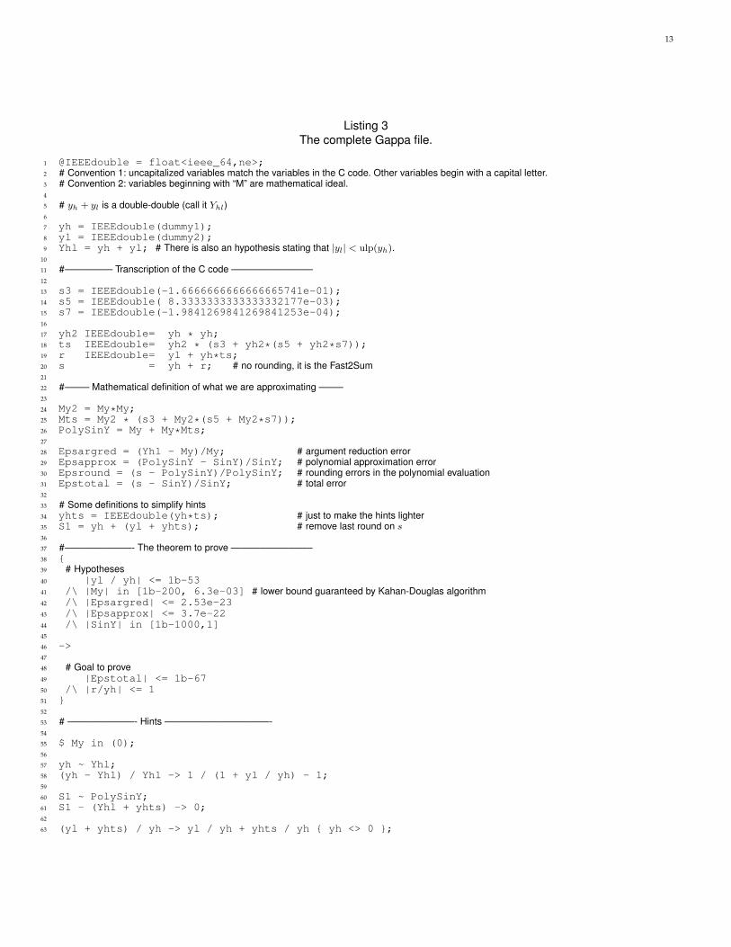
Listing 3The complete Gappa file.

1 @IEEEdouble = float<ieee_64,ne>;2 # Convention 1: uncapitalized variables match the variables in the C code. Other variables begin with a capital letter.3 # Convention 2: variables beginning with “M” are mathematical ideal.4

5 # yh + yl is a double-double (call it Yhl)6

7 yh = IEEEdouble(dummy1);8 yl = IEEEdouble(dummy2);9 Yhl = yh + yl; # There is also an hypothesis stating that |yl| < ulp(yh).

10

11 #————— Transcription of the C code ————————–12

13 s3 = IEEEdouble(-1.6666666666666665741e-01);14 s5 = IEEEdouble( 8.3333333333333332177e-03);15 s7 = IEEEdouble(-1.9841269841269841253e-04);16

17 yh2 IEEEdouble= yh * yh;18 ts IEEEdouble= yh2 * (s3 + yh2*(s5 + yh2*s7));19 r IEEEdouble= yl + yh*ts;20 s = yh + r; # no rounding, it is the Fast2Sum21

22 #——– Mathematical definition of what we are approximating ——–23

24 My2 = My*My;25 Mts = My2 * (s3 + My2*(s5 + My2*s7));26 PolySinY = My + My*Mts;27

28 Epsargred = (Yhl - My)/My; # argument reduction error29 Epsapprox = (PolySinY - SinY)/SinY; # polynomial approximation error30 Epsround = (s - PolySinY)/PolySinY; # rounding errors in the polynomial evaluation31 Epstotal = (s - SinY)/SinY; # total error32

33 # Some definitions to simplify hints34 yhts = IEEEdouble(yh*ts); # just to make the hints lighter35 S1 = yh + (yl + yhts); # remove last round on s36

37 #———————- The theorem to prove ————————–38 {39 # Hypotheses40 |yl / yh| <= 1b-5341 /\ |My| in [1b-200, 6.3e-03] # lower bound guaranteed by Kahan-Douglas algorithm42 /\ |Epsargred| <= 2.53e-2343 /\ |Epsapprox| <= 3.7e-2244 /\ |SinY| in [1b-1000,1]45

46 ->47

48 # Goal to prove49 |Epstotal| <= 1b-6750 /\ |r/yh| <= 151 }52

53 # ———————- Hints ———————————-54

55 $ My in (0);56

57 yh ~ Yhl;58 (yh - Yhl) / Yhl -> 1 / (1 + yl / yh) - 1;59

60 S1 ~ PolySinY;61 S1 - (Yhl + yhts) -> 0;62

63 (yl + yhts) / yh -> yl / yh + yhts / yh { yh <> 0 };

14

[34] F. de Dinechin, C. Q. Lauter, and G. Melquiond, “Assisted verifi-cation of elementary functions,” LIP, Tech. Rep. RR2005-43, Sep.2005.

[35] C. Q. Lauter and F. de Dinechin, “Optimising polynomials forfloating-point implementation,” in 8th Conference on Real Numbersand Computers, Jul. 2008, pp. 7–16.

Florent de Dinechin was born in Charenton,France, in 1970. He received his DEA fromthe École Normale Supérieure de Lyon (ENS-Lyon) in 1993, and his PhD from Université deRennes 1 in 1997. After a postdoctoral posi-tion at Imperial College, London, he is now apermanent lecturer at ENS-Lyon in the Labora-toire de l’Informatique du Parallélisme (LIP). Hisresearch interests include computer arithmetic,software and hardware evaluation of elementaryfunctions, computer architecture and FPGAs.

Christoph Lauter was born in Amberg, Ger-many, in 1980. He received a MSC degree inComputer Science from Technische UniversitätMünchen, Germany, in 2005, and his PhD de-gree from École Normale Supérieure de Lyon,France, in 2008. He is member of the Numer-ics Group at Intel Corporation, Hillsboro, Ore-gon, USA. His research interests include cor-rect rounding of elementary functions, computerarithmetic, computer algebra, numerical analysisand emulation of future hardware products.

Guillaume Melquiond was born in Nantes,France, in 1980. He received the MSC andPhD degrees in Computer Science from theÉcole Normale Supérieure de Lyon, France, in2003 and 2006. After a postdoctoral position atthe Microsoft Research–INRIA joint center, heis now a researcher for the INRIA Saclay–Île-de-France in the ProVal team of the Labora-toire de Recherche en Informatique (LRI), Orsay,France. His research interests include floating-point arithmetic, formal methods for certifying

numerical software, interval arithmetic, and C++ software engineering.