CFCM CENTRE FOR FINANCE AND CREDIT MARKETS

Working Paper 09/05

Time to Build Capital: Revisiting Investment-Cashflow Sensitivities

John Tsoukalas

Produced By: Centre for Finance and Credit Markets School of Economics Sir Clive Granger Building University Park Nottingham NG7 2RD Tel: +44(0) 115 951 5619 Fax: +44(0) 115 951 4159 enquiries@cfcm.org.uk

Time to Build Capital: Revisiting Investment-CashFlow Sensitivities

John D. TsoukalasSchool of Economics, University of Nottingham, University Park, Nottingham, NG7 2RD

This draft: May 2009

Abstract

Is cash flow important in explaining investment dynamics? A large body of empiricalwork argues that it is. This finding is further taken as evidence of capital marketimperfections. We argue that time-to-build for capital projects creates an investmentcash flow sensitivity as found in empirical studies that may not be indicative of capitalmarket frictions. We demonstrate this using a perfect capital markets model withfirms that make investment decisions in capital projects indexed by the length of thetime-to-build. We show that the typical (empirical) investment regression with q andcash flow is ridden with specification error under time-to-build investment. This erroris due to an omitted right hand side state variable (current expenditure on existingcapital projects) that fully describes optimal investment along with marginal q and isstrongly correlated with cash flow. In addition, time aggregation error can give riseto cash flow effects independently of the time-to-build effect. Importantly, both errorsarise independently of potential measurement error in q.

JEL classification: D21; E22; E32; G31.

Key words: Investment; Capital market imperfections; Time-to-build.

This paper is based on Chapter 2 from my 2003 PhD dissertation at the University of MarylandCollege Park. I am grateful to John Haltiwanger, Michael Pries, Plutarchos Sakellaris and JohnShea for inspiration, encouragement and valuable suggestions. I would also like to thank colleaguesfrom the Bank of England, Spiros Bougheas, Paul Mizen, Hashmat Khan and seminar participantsat the Bank of England and Cardiff Business School.Email: john.tsoukalas@nottingham.ac.uk

1 Introduction

Investment in fixed capital is one of the most important and volatile components of aggregate ac-

tivity. Understanding investment dynamics is central to the study of aggregate fluctuations. In the

neoclassical theory of firm investment with adjustment costs, the firm’s market value and invest-

ment respond simultaneously to signals about future profitability as encoded in Tobin’s q. In this

theory, Tobin’s q, defined as the expected value of the firm relative to its capital stock becomes a

summary statistic for investment. Nevertheless, despite its theoretical appeal the empirical perfor-

mance of the q theory has been rather disappointing; the explanatory power of q is found to be low

and the responsiveness of investment to fundamentals rather weak. Moreover, various measures of

internal funds such as profits or cash flow are found significant in explaining corporate investment.

This finding is further taken as evidence of capital market imperfections that disturb the firm’s

investment schedule from the frictionless neo-classical benchmark. This paper uses a neoclassical

investment-q model with time-to-build and time-to-plan features for capital and revisits this evi-

dence. When time is required to build new capital q is no longer a sufficient statistic for investment

because this technology implies an additional state variable significantly affects optimal investment.

The fact that q in this case cannot adequately control for fundamentals casts doubt on the evidence

established in a large body of work, namely that the sensitivity of investment to cash flow is a sign

of capital market frictions.

Time-to-build and time-to-plan are key technological features of investment. A variety of survey

(Montgomery (1995) and Koeva (2000)) and firm level (Koeva (2001), Del Boca et al. (2008))

evidence suggests that these technological constraints are important at the firm level. The available

evidence indicates that the time required for the installation of new equipment and structures

ranges from 3 to 4 quarters for equipment and 2 to 3 years for non-residential structures. But as we

demonstrate in this paper the typical investment-q empirical equation that serves as the benchmark

for evaluating the capital market imperfections hypothesis, is usually not robust to the presence

of time-to-build investment. It is thus important to investigate the effects of time-to-build in the

pure neoclassical investment-q framework, that has been pioneered by Tobin (1969), extended by

Hayashi (1982) and being widely used in empirical work since. This is our main goal in this paper.

The importance of time-to-build in the context of the neoclassical investment-q equation was

first examined by Barnett and Sakellaris (1999). Barnett and Sakellaris (1999) estimate, using

firm-level data, that investment responds strongly to fundamentals when a measure of q consistent

with the time-to-build evidence is used in the empirical equation. Time-to-build as originally

articulated in Kydland and Prescott (1982) (KP) seminal paper has recently re-emerged in the

1

business cycle literature with considerable success in explaining a variety of empirical facts. Gomme

et al. (2001) use it to explain the co-movement of household and market capital stocks. Edge (2007)

demonstrates that a variant of the KP assumption can give rise to an empirically plausible liquidity

effect in a sticky-price monetary model. In Wen (1998) and Zhou (2000) time-to-build becomes

critical in explaining aggregate investment dynamics and the persistence of output fluctuations

and in Bernanke et al. (1999) and Casares (2006) to explain the delayed response of investment to

various shocks.

We use the model to calibrate and simulate an industry to the aggregate U.S. manufacturing

sector and use it as a laboratory to study the role of cash flow in investment regressions. We

analyze the role of time-to-build technology for capital in explaining the emergence of significant

cash flow effects in linear investment-q equations. In our model capital markets are perfect yet an

important cash-flow effect arises in our simulated investment regressions, replicating what is found

in many empirical studies (see for e.g. Fazzari et al. (1988), Gilchrist and Himmelberg (1995),

and the survey by Hubbard (1998)). Based on our findings we argue that the cash flow sensitivity

of investment may not be a useful indication for the existence and importance of capital market

imperfections for investment dynamics.

Our results closely corroborate findings reported in Eberly et al. (2008). We identify specifica-

tion error that renders q an insufficient summary statistic as the primary driver of cash flow effects

in investment-q regressions although (as explained below), in contrast to Eberly et al. (2008) our

findings are free of measurement error in q. Nevertheless as we demonstrate, measurement error

magnifies the specification error we identify. Further, our model provides an explanation for the

emergence of lagged investment effects in empirical investment-q regressions, in addition to cash-

flow effects. The importance of lagged investment effects is a largely overlooked empirical regularity,

since most of empirical work focuses almost exclusively on the role of cash flow. But as Eberly

et al. (2008) note: “Both cash-flow and lagged-investment effects have been found in virtually every

investment regression specification and data sample.” In our study—as in Eberly et al. (2008)—we

show that the lagged investment rate is an important determinant of current investment because it

proxies for an omitted state variable. In Eberly et al. (2008) simulations, lagged investment proxies

for a regime-switching component in a firms’ demand. In the present model with time-to-build,

lagged investment has a different structural interpretation, capturing time-to-build effects for the

construction of capital. The role of this omitted state variable is crucial for the emergence of

cash-flow effects in our simulated panel data regressions.

The mis-specification in investment-q equations under the presence of time-to-build technology

for capital goods arises as a result of an omitted state variable that belongs to the set of explana-

2

tory variables—in addition to q—and is strongly correlated with cash flow. With time-to-build,

marginal q is not a sufficient statistic for investment. Investment consists of new and partially-

finished projects that have not yet become productive capital. In addition to q the sum of current

expenditures on existing projects belongs to the right hand side of the investment regression. In

other words, when the firm decides—on the basis of new information about future investment

opportunities—how many new projects to initiate, past projects already under way influence that

decision, i.e. they constitute a state variable. We furthermore derive the correct specification under

time-to-build and show that we can approximate this omitted state variable with a simple (and

easily constructed) variable that is a function of the lagged investment rate and the growth rate of

the capital stock. We evaluate the usefulness of this approximation for empirical work in our sim-

ulated environment and find that it performs almost as well as its theoretical counterpart, nearly

eliminating the cash flow effect from the investment regression. In addition, and independently of

the time-to-build effect above we show that a cash flow effect can emerge in an investment-q equa-

tion when researchers estimate an investment-q regression using annual data that are aggregated

from more frequent factor input decisions. This time aggregation error has been highlighted in

the context of capital and labor adjustment cost estimates by Hall (2004) but as far as we know

the implications in an investment-q framework have not been explored. Last, it is important to

emphasize that our results are not driven by measurement error in q. In the simulated environment

we study we use the model consistent measure of expected marginal q.

Recent work by Erickson and Whited (2000), Gomes (2001), Cooper and Ejarque (2003), Alti

(2003), Cummins et al. (2006), Abel and Eberly (2003), also cast doubt on the validity of investment

cash flow sensitivities as an indicator of capital market imperfections. Erickson and Whited (2000),

Gomes (2001) and Cummins et al. (2006) stress that cash flow effects may arise because Tobin’s

q is measured with error. Cooper and Ejarque (2003) emphasize market power that creates a

divergence between average and marginal q while in Alti (2003) Tobin’s q is a noisy measure of

fundamentals cash flow is highly informative about long-run profitability. Finally, in Abel and

Eberly (2003) cash flow effects arise as a result of specification error induced by changes in the user

cost of capital. Yet, our contribution is rather different from all the above. First, we provide a

new and important channel for the emergence of cash flow in investment-q regressions. This builds

on the time-to-build nature of investment. Second, in contrast to the studies above our findings

do not involve any mis-measurement between average and marginal q and thus are not driven by

measurement error.

The rest of the paper is organized as follows. Section 2 describes the model. Section 3 discusses

the solution and calibration. In Section 4 results from the simulated version of the model are

3

presented. Section 5 concludes.

2 The Model

We use a model suitable for analyzing firms investment decisions in a time-to-build environment.

A similar framework has been employed by Zhou (2000) to explain aggregate investment dynamics.

The following subsections explain the components that are essential to the framework.

2.1 Firms

2.1.1 Technology

We model an industry which is populated by a continuum of risk-neutral infinitely-lived firms. Firm

j produces output, using the following decreasing returns to scale Cobb-Douglas technology:1

yjt = AtωjtF (Kjt,Mjt, Ljt) = AtωjtKαjtM

γjtL

νjt γ + α + ν < 1

where At is an aggregate (common) and ωjt an idiosyncratic productivity shock. Kjt is capital, Ljt

is the labor input and Mjt is the stock of materials.

The investment technology requires time to build new capital. Specifically, it takes J-periods

(stages) to build new productive capacity. This technology implies that in any given period t,

firms initiate new projects, sJt, and complete partially finished projects, sit, i 6= J at stage i.

This assumption intends to capture the design and construction (delivery) stages that exist in

undertaking investment projects in plant and equipment as suggested by Kydland and Prescott

(1982). The assumptions of this time-to-build (TTB) technology are summarized below:

sit = si−1,t+1 i = 2, ...J (2.1)

Kt+1 = (1− δ)Kt + s1t (2.2)

It =J∑

i=1

ϕisit (2.3)

with 0 ≤ ϕi ≤ 1, i = 1, 2, ...J , and∑J

i=1 ϕi = 1. To clarify notation, sJt denotes new projects at

time t, sJ−1,t denotes projects initiated at time t− 1, that are J − 1 periods away from completion

at time t, and so on. The last stage project, s1t yields productive capital in the following period.

1Decreasing returns to scale are necessary for firm size to be well defined. Otherwise firm size is indeter-minate and the entrepreneurial sector reduces to just a single producer.

4

The parameters ϕi determine the fixed fraction of resources allocated to projects that are i periods

away from completion, or equivalently the proportion of the value of the project put in place in

period i. It denotes total investment expenditures at time t and depends on the resources expended

for the different incomplete projects. Finally, the capital stock depreciates at rate δ.

New investment projects are subject to adjustment costs. It is assumed that firms face a

quadratic cost of adjustment function for investment in new projects, i.e.,

G(sJ,jt,Kjt) =η

2(sJ,jt

Kjt− δ)2Kjt (2.4)

where the parameter η governs the curvature of G.2 This function has all the usual properties,

i.e., it is convex, with a rising marginal adjustment cost. It also implies a zero adjustment cost in

the steady state.

The decision relating to the materials input is as follows. The firm places materials orders djt,

for use in production in period t + 1, Mjt+1. The stock of materials thus evolves according to:

Mjt+1 = (1− δm)Mjt + djt (2.5)

where δm denotes the depreciation rate for materials. Note that this timing convention assumes

that orders of materials at time t enter the firm after current production has taken place.

Last, firms hire labor from a competitive market at a given (constant) wage rate, w.

2.1.2 The firm’s problem

Timing is as follows. At the beginning of period t, the idiosyncratic (ωjt) and aggregate productivity

shocks (At) are observed. The firm inherits a stock of capital Kjt, materials Mjt, and partially-

completed projects s1,jt, s2,jt, ...s(J−1),jt, from the previous period. Then, before At+1 and ωj,t+1

are observed, the firm chooses new investment projects, sJ,jt, materials orders, djt, and labor input,

Ljt, in order to maximize firm value.

maxLjt,sJ,jt,djt

E0

∞∑

t=0

βtdivjt

where divjt denote dividends and β = 11+r is the market discount factor, where r denotes the risk

free rate.3Note that the firm’s uses and sources of funds equation defines dividends:

2An alternative characterization of the adjustment cost function is to assume that the cost is paid atthe time when resources on projects are expended, i.e., G(s1,jt, ...sJ,jt,Kjt) =

∑Ji=1 ϕi

η2 ( si,jt

Kjt− δ)2Kjt. We

choose to work with the simpler form (2.4) because of the analytical simplicity. We nevertheless presentresults using this functional form assumption as well.

3Notice that the use of the risk free rate in the discount factor implies that the firm’s financing choicesare irrelevant to its investment decisions. Moreover the presence of materials is inconsequential for ouranalysis but we have chosen not to maximize out this factor of production in order to be consistent with our

5

divjt = AtωjtKαjtM

γjtL

νjt − wLjt − djt − Ijt −G(sJ,jt,Kjt) (2.6)

The laws of motion for the exogenous state variables are described below.

lnAt+1 = ρAlnAt + σAεAt+1 εA

t ∼ N(0, 1) (2.7)

lnωj,t+1 = ρωlnωj,t + σωεωj,t+1 εω

j,t ∼ N(0, 1) (2.8)

Last we note that profits are defined as:

πj,t = AtωjtKαjtM

γjtL

νjt − wLjt (2.9)

The maximization is subject to (2.1)—(2.8) and the given initial values for the state variables.

The firm’s problem defined above can be described in 4 plus J−1 state variables (K, M, {si}J−1i=1 , A, ω).

Given the high dimensionality of this problem a solution based on a global approach (e.g. policy or

value function iteration), will be infeasible for a reasonably accurate characterization of the solution

(curse of dimensionality). To circumvent this difficulty a second order approximation method is

used.

We can write the Langrangean for the problem,

maxLt,sJt,dt

E0

∞∑

t=0

βt{divt + qt(Kt+1 − (1− δ)Kt − s1t) + µt(Mt+1 − (1− δm)Mt − dt)}

where qt, µt denote the Kuhn-Tucker multipliers associated with the equality constraints (2.2)

and (2.5). Note that the multiplier qt represents the shadow value of installed capital, i.e., marginal

q that captures the future expected marginal profitability of a unit of capital (contributing both to

profits and the reduction in adjustment costs). The assumptions of our model imply that expected

marginal q is a sufficient statistic for investment in new projects, sJ,jt. Assume that projects require

3 periods to completion. Then it can readily be shown that the optimal investment rate obeys:

Ij,t

Kj,t= ϕ3

(− 1

η(ϕ3 + βϕ2 + β2ϕ1) + δ

)+ ϕ3

1ηβ2Et(qj,t+2) +

2∑

i=1

ϕisi,jt

Kj,t

Optimal investment is a function of future expected marginal q, reflecting the fact that capital

will become productive with a lag and an additional state variable that represents part of the

investment outlays already underway. Thus in this environment q ceases to be a sufficient statistic

for investment. To conserve space the complete description of the first order necessary conditions

that characterize an optimum for this problem are given in Appendix 1.

calibration procedure.

6

3 Solution

The equilibrium of the model is characterized by a set of Euler equations along with the Kuhn-

Tucker conditions for the equality constraints and the given initial values for the state variables.

This equilibrium is a set of non-linear equations and an analytical solution is infeasible to compute.

An approximate solution is calculated by using a second order approximation method around the

non-stochastic steady state of the model. The second order Taylor approximation, as described

in Schmitt-Grohe and Uribe (2004), can be readily used to calculate the decision rules for new

projects, materials orders and labor.4

3.1 Calibration

In order to analyze the equilibrium we calibrate the model using a baseline set of parameter values

as in Table 1. We calibrate the parameters needed to simulate our model to characteristics of the

U.S. manufacturing sector.

The values for the output elasticity of materials, γ, labor, ν and capital, α are taken from the

manufacturing plant level study of Sakellaris and Wilson (2004) (Table 1, p.15, C). These values

imply an overall returns to scale equal to 0.98. This value is consistent with Basu and Fernald

(1997) estimates of the returns to scale in manufacturing. There is a variety of empirical evidence

of time-to-build for capital projects. Regarding equipment investment, Abel and Blanchard (1986)

document an average delivery lag for manufacturing firms equal to three quarters (during which

time they pay installments for the purchase of the capital good). Mayer and Sonenblum (1955)

report that the average time across industries needed to equip plants with new machinery is 2.7

quarters. Montgomery (1995) examines a long series of finely detailed surveys conducted by the

U.S. Department of Commerce on TTB patterns for a wide range of firm construction projects.

His calculations imply a time-to-build between five to six quarter for non-residential structures.

There is still evidence of lengthier construction times for non-residential structures. According

to Mayer (1960) and Koeva (2001) it takes approximately two years to complete non-residential

structures. A recent study by Del Boca et al. (2008) using Italian firm level data suggests that

investment projects require 2-3 years from initial stage to completion, while equipment investment

becomes productive within a year. Based on this evidence and given the fact that the model’s

empirical counterpart is total capital we think that three or four quarters is a reasonable length

for the time-to-build assumption. We set the length of the time-to-build equal to three quarters

(J=3) in our baseline calibration but we also discuss results varying this value up to four quarters.

4Appendix 1 outlines the essential computational details of the solution.

7

In terms of the resources spent on each stage of the construction (or installments for delivery)

Kydland and Prescott (1982) assume an equal cost distribution. Recently, Zhou (2000) argues

that time-to-build is very important for explaining investment dynamics. He estimates ϕi for

various values of J and reports that an (approximately) equal distribution of cost for time-to-

build investment produces the best fit for aggregate U.S. investment. There also exist estimates

(e.g. Del Boca et al. (2008)) particularly for investment in structures that point to initial planning

phases with little or no resources spent followed by construction phases with increasing resources

as projects near completion. This pattern of spending is known as time-to-plan (TTP). For the

baseline calibration we set ϕ1 = ϕ3 = 0.333, ϕ2 = 0.34 and explore TTP in the simulations as an

alternative scenario. The parameter that governs the convexity of the adjustment cost function, η

is set equal to 1.08 at the quarterly rate. This parameter is estimated by Barnett and Sakellaris

(1999) using a Tobin’s q approach in a panel of manufacturing firms from 1959 to 1987 (see Table

3 p.256). In implementing their approach the authors assume a time-to-build of one year thus

closely corresponding to our assumptions. The magnitude of (convex) adjustment costs estimated

by Barnett and Sakellaris (1999) and more recently by Cooper and Haltiwanger (2006) seem to be

conforming much better to the q theory of investment compared to earlier estimates that produced

implausibly large adjustment cost estimates (See for example, Hayashi (1982), or Summers (1981)).5

We also experiment with several alternative values for η taken from these studies. The subjective

discount factor, β, is chosen to match the average risk-free real interest rate over the period 1947Q1

to 2006Q2. The real interest rate is defined as the 3-month U.S. T-bill rate less consumer price

inflation. The depreciation rate for materials is calculated as follows. The stock of materials at the

end of a quarter is (1−δm)Mt. Usage of materials in quarter t is δmMt. Since usage is not available

quarterly but only annually we use the following approximation. usageyq = usagey

outputy outputyq , where y

denotes year and q quarters. This calculation should be sufficiently accurate since materials usage

and output are highly correlated and their ratio will thus be quite smooth in the short-run. The

data used for this calculation are available from the Annual Survey of Manufacturers (ASM) and the

NBER manufacturing productivity database. δm is then calculated from the restriction (1−δm)Mt

δmMt=

materials inventories at end quarter tusage of materials in quarter t . In the data (1962-2000) the ratio is on average equal to

0.33. The calculation implies δm = 0.75. We set δ the fixed capital depreciation rate to 0.025 per

quarter. We calibrate the process for the idiosyncratic productivity shock, ρω, σω to match the

autocorrelation and standard deviation of (cyclical) aggregate manufacturing investment. Finally,

5We choose to work with these recent (more realistic) estimates for another reason. A higher adjustmentcost parameter η would imply a greater positive serial correlation of investment that would (in the presenceof autocorrelated productivity) be more strongly correlated with profits, thus making it easier to obtain asignificant profit rate coefficient in a mis-specified regression.

8

we calibrate the process for the aggregate productivity shock, ρA, σA to match the autocorrelation

and standard deviation of (cyclical) aggregate manufacturing output. The data for this calculation

(manufacturing investment and output) are taken from the Bureau of Economic Analysis and cover

the period 1967 II to 2004 IV.

4 Results

In this section, we present results from the calibrated version of the model. The (approximate)

decision rules for the model’s variables are simulated and artificial data are generated. Using the

artificial data we create a panel of firm level data. We run investment-q regressions on the panel

and discuss the role of cash flow.

4.1 Investment-q regressions

Empirical studies that emphasize the role of capital market imperfections in explaining the cyclical

behavior of investment utilize firm-level data and typically regress fixed investment to a set of

explanatory variables that includes a proxy for changes in net worth. For example in Fazzari et al.

(1988) or Gilchrist and Himmelberg (1995) the q theory of investment is augmented (and tested)

with measures of internal funds (profits or cash-flow). These studies demonstrate the significance of

these measures in explaining fixed investment. A typical finding is a significant cash-flow coefficient

along with a very large estimate for the adjustment cost parameter. This is interpreted as evidence

of capital market frictions and a rejection of the q theory of investment. This section presents results

obtained from our simulated industry, and raises questions about the validity of this interpretation.

We generate a panel of 1000 firms observed over 20 years and demonstrate that a significant cash-

flow effect can arise even in a model with perfect capital markets.

Previous work has also reached similar conclusions. Gomes (2001) questions the validity of cash-

flow as an indication of capital market imperfections using a structural model. He concludes that

a cash-flow effect may arise as a combination of measurement error and identification problems in

a linear regression framework. Erickson and Whited (2000) and Cummins et al. (2006) emphasize

measurement error in Tobin’s q, while Cooper and Ejarque (2003) argue for market power that

induces a divergence between marginal and average q. Finally, in Abel and Eberly (2003) cash-flow

is a proxy for an (unobserved) time-varying depreciation rate and in Eberly et al. (2008) cash flow

arises because it proxies for the regime in demand which is a state variable for investment. In our

model of course decreasing returns to scale imply that average q differs from marginal q. But our

contribution does not rely on the mis-measurement between average and marginal q. Instead the

cash flow sensitivity of investment in our framework has its root in the technology for investment

9

projects and the specification error it creates in the typical investment-q regression. In the analysis

below we make use of the theoretically correct measure of marginal q (section 4.5 studies the

implications of adding measurement error in q).

We note that empirical studies including those mentioned above as well as most others we are

aware of typically rely on annual firm level (e.g. Compustat) data, whereas our model is calibrated

quarterly. We first present brief results to build intuition using our quarterly model and then

aggregate our model to correspond to the annual frequency.

To demonstrate the inference-problem associated with reduced form investment equations under

time-to-build, we estimate an OLS regression on the artificial data (for J = 3),

Ij,t

Kj,t= α + b1Et(qj,t+2) + b2

πj,t

Kj,t+ εj,t (4.1)

where the left-hand-side (LHS) variable is the investment rate, and the right-hand-side (RHS)

variables are the expected marginal q along with the profit rate. Expected marginal q is the correct

statistic for capturing future investment opportunities under TTB because new investment projects

become productive after three periods (see the FOC for new investment projects in Appendix 1).

This is a typical empirical investment equation except that Tobin’s q is usually taken as a proxy

for the un-observed marginal q.6 A notable exception is Gilchrist and Himmelberg (1995) who

construct a proxy for marginal expected q. We contrast this equation with the equation implied

by the first order condition (FOC) for project starts for J = 3,

sJ,jt

Kj,t= −1

η(ϕ3 + βϕ2 + β2ϕ1) + δ +

1ηβ2Et(qj,t+2) (4.2)

which using the definition of Ij,t from (2.3) can be re-written as,

Ij,t

Kj,t= ϕ3

(− 1

η(ϕ3 + βϕ2 + β2ϕ1) + δ

)+ ϕ3

1ηβ2Et(qj,t+2) +

2∑

i=1

ϕisi,jt

Kj,t(4.3)

Comparing equation (4.1) with (4.3) we can observe (ignoring the constant and error term) that

the correct specification under TTB includes∑2

i=1 ϕisi,jt

Kj,tas a RHS variable. This sum is the part

of investment that has responded to old information (about productivity) and is therefore a state

variable. The question is whether omitting this variable invalidates the inference drawn on the

role of profits from an empirical equation like (4.1). The answer is affirmative if the profit rate is

correlated with∑2

i=1 ϕisi,jt

Kj,t. This turns out to be the case with persistent productivity shocks.7 The

6We note that a typical empirical equation also includes a firm specific effect. In our model firms canonly differ in the history of shocks they receive so there is not any ex-ante firm-specific heterogeneity.

7To conserve space we present a set of correlations in section 4.2. For the case examined here thecorrelation between the two series is equal to 0.83.

10

intuition is as follows. Suppose that at some time in the past a favorable productivity shock caused

a surge in new projects. As time elapses these new projects come closer to completion time and if

the shock is persistent then at time t there will be a series of outstanding projects, s1ts2t, ..., sJ−1,t.

Moreover with persistent shocks current profits will also reflect the same past productivity shocks

that caused the firm to initiate new projects and are now exactly those projects above that have

moved closer to completion. Therefore current profits are correlated with each of these previous

capital projects and hence their sum. This implies that profits will proxy for this state variable in

an investment-q regression. Of course if q was a sufficient statistic for total investment (as evident

from equation (4.2) it is a sufficient statistic only for new projects, sJt) then profits would not

be significant in a regression with investment and q. Table 2 reports the results from estimating

equation (4.1) on our artificial panel of firms. We can observe that the profit rate coefficient, b2

is positive and statistical significant, even though our model was designed without capital market

imperfections. Therefore, the profit rate appears as a significant variable and improves the fit of

the equation as it proxies for a relevant omitted RHS variable. It is also important to stress that

any role for this variable in these regressions does not arise as a result of measurement error since

we are using the appropriate (marginal) measure of q. Instead the explanatory role of the profit

rate arises as a result of specification error due to TTB for investment.8

4.2 Time aggregation

We wish to know the implications of our TTB assumption and the validity of our simulated re-

gression results on the role for profits when we aggregate our model. We previously indicated that

most empirical studies use annual firm-level data. We therefore aggregate our artificial data to

correspond to the same annual measures used in these studies and make the investment equations

directly comparable. Our timing assumptions imply investment decisions that are taken quarterly.

The use of annual data on the other hand implies annual factor input decisions. We view the

quarterly frequency much more realistic given the flow of information upon which decisions are

taken. Hall (2004) argues that decisions concerning factor employment are made more frequently

than once a year (quarterly or even monthly) and analyzes how time aggregation biases capital

adjustment cost estimates when annual data are used in estimation. In this section we have two

goals. First, in view of Hall (2004) findings to explore whether time aggregation can spuriously

assign a role to cash flow independently of the specification error that is created as a result of TTB.

Second, to investigate precisely how the TTB specification error generalizes in this framework. To

8As expected, if we estimate the correct specification (4.3) we find no role for the profit rate. We do notreport these results for brevity but they are available upon request.

11

preview the results we highlight two findings: (i) we identify a time aggregation error that can

give rise (independently from the specification error from TTB) to cash flow effects in investment

regressions with annual data and (ii) we demonstrate that the TTB specification error generalizes

in the annual environment.

To obtain annual from quarterly measures we adopt the same methodology as in the national

accounts and employed by Hall (2004). Specifically, we set all the flow variables at the annual rate

equal to the sum of the corresponding flow variables over the quarters, i.e., for flow variable x,

xat =

∑4k=1 xt,k, where x = I, π, si, , i = 1, ...J and a denotes annual frequency.

The annual measure for marginal q, is the average over the corresponding quarterly measure.

However, it differs slightly depending on the TTB. We use the following definitions9

J = 1 , qat =

∑4k=1 qt,k

4, J = 2 , qa

t =∑4

k=1 Ekqt,k+1

4

J = 3 , qat =

∑4k=1 Ekqt,k+2

4, J = 4 , qa

t =∑4

k=1 Ekqt,k+3

4

Finally, we take the annual capital stock to correspond to the end of year (i.e. fourth quarter)

stock.10

We then re-estimate the empirical investment equation specified in section 4.1 using the annual

measures derived above (for convenience we drop the firm-specific subscript j), for J = 1, 2, 3, 4.

Here as in the previous section J refers to TTB in quarters, so the maximum length for the

construction of capital we consider is one year.

Iat

Kat

= α + b1qat + b2

πat

Kat

+ εat (4.4)

Table 3 reports the results from estimation of (4.4). There are two noteworthy findings. First,

the adjustment cost estimate derived from b1 is upward biased (top panel of Table 3, imposing

b2 = 0). Second, adding the profit rate to the regression yields a positive and statistical significant

b2 coefficient (bottom panel). We discuss these findings in detail later in this section. We now

focus on the question whether the explanatory power of ( πat

Kat) is due to time aggregation and/or

specification error resulting from the time-to-build nature of investment. We can decompose the

two sources of error to answer this question. First, notice from Table 2 that for J = 1 in the

quarterly model, ( πtKt

) has no explanatory power. This follows from the fact that for J = 1 there

9In general∑4

k=1 Ekqt,k+J−1

4 6=∑4

k=1 qt,k

4 . However, with autocorrelated productivity shocks the two mea-sures are highly correlated. We use the marginal expected q for each different J to isolate the omittedvariable effect. Our results are broadly similar if we use the same q for each J .

10Alternatively, the annual measure for the capital stock can be calculated from Kat+1 = (1− δa)Ka

t + sa1t.

The results presented in this section are insensitive to this alternative definition.

12

is no investment outlay that refers to a decision taken previously (sJt = ... = s1t = It) and hence

no omitted RHS state variable. Even though the profit rate will be correlated with investment

rates, its forecasting role for future investment opportunities is properly accounted for by marginal

q. Thus any role for the profit rate in Table 3 in the J = 1 column can be solely attributed to the

time aggregation error. We can derive an expression for the time aggregation error if we write the

first order condition for investment (for J = 1),

−1− η(Ik

Kk− δ) + qk = 0

Since this must be satisfied in any quarter k = 1, 2, 3, 4, it follows from aggregation over quarters,

−4− η

( 4∑

k=1

(It,k

Kt,k− δ)

)+

4∑

k=1

qt,k = 0

where t denotes years. In Appendix 2 we show that after suppressing the constant terms the

equation above can be written as,

Iat

Kat

= constant +(

1Ka

t

4∑

k=1

It,k

Kt,kKt,k −

4∑

k=1

It,k

Kt,k

)+

1ηa

qat (4.5)

The time aggregation error is the term in parenthesis,(

1Ka

t

∑4k=1

It,k

Kt,kKt,k −

∑4k=1

It,k

Kt,k

). This

term will be different from zero except when investment is equal to replacement investment and

thus Kat = Kt,k. Moreover, this term will be correlated with the profit rate since it is a function

of investment rates. Thus the aggregation of more frequent investment decisions results in a small

but positive profit rate coefficient as found in Table 3. On the other hand, the specification error

that arises due to the TTB nature of investment can be seen by examining the FOC for optimal

investment when J > 1. For example, summing the FOC for optimal investment for J = 3 we get,

−4(ϕ3 + βϕ2 + β2ϕ1)− η

( 4∑

k=1

(s3t,k

Kt,k− δ)

)+ β2

4∑

k=1

Ekqt,k+2 = 0

which after repeating the steps above and using (2.3) we can write as,

−(ϕ3 + βϕ2 + β2ϕ1)− η

4

( 4∑

k=1

(It,k

Kat

− δ))

+η

4

(1

Kat

4∑

k=1

It,k

Kt,kKt,k −

4∑

k=1

1ϕ3

It,k

Kt,k

)

+η

4ϕ3

4∑

k=1

∑2i=1 ϕisit,k

Kt,k+ β2

∑4k=1 Ekqt,k+2

4= 0

Re-arranging this equation to bring Iat

Kat

on the left hand side of the equation we finally arrive

at,

13

Iat

Kat

= constant +(

1Ka

t

4∑

k=1

It,k

Kt,kKt,k − 1

ϕ3

4∑

k=1

It,k

Kt,k

)+

1ϕ3

4∑

k=1

∑2i=1 ϕisit,k

Kt,k+

1ηa

β2qat (4.6)

where again we have used,∑4

k=1It,k

Kat

= Iat

Kat

and qat =

∑4k=1 Ekqt,k+2

4 . We see that relative to

(4.5), there is an additional RHS variable that reflects the TTB technology. This is given by∑4

k=1

∑2i=1 ϕisit,k

Kt,kwhich is a summation (over quarters per year) of the omitted state variable in

equation (4.3), i.e. a linear combination of the latter. The annual profit rate, ( πat

Kat), will be the sum

of the corresponding quarterly rates and it will be correlated with this state variable since both are

sums of the corresponding quarterly measures. Therefore since the profit rate is correlated with

the key omitted state variable and the investment rate (see Table 4, lower bottom) regressing Iat

Kat

on qat and the profit rate will result in a statistical significant role for the latter. But this is merely

reflecting the omission of an explanatory variable from the RHS of the regression.11 Since in our

model capital markets are perfect, any role for profits must result from this mis-specification.

We now discuss the results reported in Table 3. In the top panel we demonstrate the bias in the

adjustment cost parameter, ηa (imposing b2 = 0). This follows from standard econometric results

since marginal q and the omitted state variable are correlated (e.g. Judge et al. (1985), p.858).

The time aggregation error is illustrated in the bottom panel of Table 3 for J = 1. This results

in a small positive profit rate coefficient as explained above.12 We also note that in the regression

excluding the profit rate the magnitude of the bias in ηa ranges from roughly 7% for J = 1 to 22%

for J = 4 (top panel, Table 3). Thus lengthier time-to-build technology will produce adjustment

cost estimates that imply slower adjustment speeds for capital. Empirical work with the q model

has been unsatisfactory (see Chirinko (1993) for a review) producing implausibly large adjustment

cost estimates. Our results offer a potential explanation for these estimates since TTB implies an

upward bias in the adjustment cost estimate. The increase in the bias reflects almost entirely the

differences in the true coefficient —equal to 1ϕJ

—of∑4

k=1

∑2i=1 ϕisit,k

Kt,k, which is rising as J ↑ and the

fact that the discount factor is also reflected in b1 (see equation (4.6))—although the latter makes

very little difference for the size of the bias. To give a sense of comparison for the bias, we note

that when only time aggregation is taken into account (for J = 1) our results are consistent with

11The estimated coefficients in Table 3 reflect both the time aggregation and specification error. However,the former’s contribution to the b2 estimates for J > 1 is extremely small. This can be shown by using∑4

k=1It,k

Kt,kinstead of Ia

t

Kat

as the LHS variable in (4.6) thus eliminating the aggregation error. The resultingestimated coefficients are nearly identical to those shown in Table 3 and are not reported but are availableupon request. In Table 3A we also report a set of regression results that use the alternative adjustment costformulation, i.e. G(s1,jt, ...sJ,jt,Kjt) =

∑Ji=1 ϕi

η2 ( si,jt

Kjt− δ)2Kjt. Results from Table 3A are qualitatively

similar.12If we regress

∑4k=1

It,k

Kt,kon

∑4k=1 qt,k. eliminating the time aggregation term, πa

t

Kat

looses its significanceand explanatory power.

14

the estimate for the bias in ηa reported in Hall (2004). He analyzes the bias arising—in estimating

capital adjustment costs—from aggregating monthly decisions to the annual frequency. Hall (2004)

reports biases in ηa from time aggregation in the order of (approximately) 10% (see Table V,

p.920)—quite similar to the 7% we obtain in this model. Thus in this simulated environment

investment-q regressions that fail to model the time-to-build technology, produce upward biased

adjustment cost estimates in addition to the cash flow effect. Barnett and Sakellaris (1999) and

Del Boca et al. (2008) using US and Italian annual firm level data respectively, provide evidence

consistent with our findings, reporting significantly lower adjustment cost parameter estimates

when TTB investment is allowed for.

The same pattern of increasing bias is evident in the bottom panel of Table 3 that includes

the profit rate as an additional RHS regressor. Most importantly, a notable finding is the close

association between the size of the bias in the adjustment cost estimate and the magnitude of the

profit rate coefficient. As we increase the length of TTB (moving from left to right) in the bottom

panel of Table 3, we observe a positive relationship between η̂a(inverse of b1 reported in the Table)

and b2. In other words, the regression results indicate higher sensitivity of investment to profits

is associated with higher adjustment cost estimates as the length of TTB increases. This result

can be simply explained since the mean value of both coefficients moves in proportion with the

true coefficient of the omitted state variable which equals 1ϕJ

(Appendix 2 provides the details).

According to omitted variables result from standard econometrics the mean value of the profit rate

coefficient reported in Table 3 will vary proportionately with the true coefficient of∑4

k=1

∑2i=1 ϕisit,k

Kt,k

given by 1ϕJ

. As long as ϕJ falls with J , that is as long as the value put in place at the first stage

of the construction falls with time required to completion, the coefficient of the profit rate will rise.

This is indeed what the evidence on TTB suggests.

What is the significance of this finding? We emphasize this result because it is closely related

to a frequent finding in empirical work with investment-q equations. In Fazzari et al. (1988)(Table

4, p.167) or Gilchrist and Himmelberg (1995) (Table 2, p.558) for example, the adjustment cost

estimate and the cash flow coefficient is noticeably larger in the group of firms that are a-priori

thought to be more vulnerable to capital market imperfections (small or low dividend payout firms)

compared to a control group, e.g. large firms. Studies typically interpret differences in cash flow

coefficients between different groups of firms as evidence of capital market imperfections. But can

the different cross sectional sensitivity of investment be explained by our perfect capital markets

model? This is the question we now turn our attention to.

15

4.3 Cross sectional implications

We have demonstrated that the TTB investment technology will produce a cash flow effect in

investment-q regressions with firm level data. We have identified a specification and a time aggre-

gation error, the former due to the TTB technology while the latter arising from aggregating more

frequent investment decisions. While we view the latter as important the focus of this paper is on

the implications of the former. We now discuss some potential cross sectional implications of TTB.

Our model predicts that the cash flow effect will be present across different cross sections of firms

as long as all cross sections share the same TTB technology. This will be true for example for small

vs. large or young vs. old firms. On the other hand studies that seek to test for the presence of

capital market imperfections typically report cash flow investment sensitivities that vary by cross

section. For instance in Fazzari et al. (1988) or Gilchrist and Himmelberg (1995) small/young

firms are estimated to have higher investment cash flow sensitivities compared to large/old firms

and the differences are interpreted as arising from capital market frictions that affect the former

significantly more than the latter. Evidently our model predicts the same cash flow sensitivity for

either small or large firms if they use the same TTB technology. The length for TTB however

will crucially depend on the type of investment that firms undertake. Consider for example two

firms (A and B) that are identical in all other respects except that firm A invests proportionally

more in structures and less in equipment compared to firm B. The available evidence discussed in

section 3.1 suggests that TTB is considerably longer for structures than it is for equipment and

by a wide margin. Therefore firm A will be characterized by a longer TTB technology compared

to firm B. Our model then predicts a larger cash flow coefficient for firm A compared to firm B.

Table 3 illustrates this. Looking across Table 3 we note that the profit rate coefficient rises with

the length of TTB. For example, the profit rate coefficient rises from 0.03 to 0.22 as we move from

1 quarter to 2 quarters, and from 0.22 to 0.29 as we move from 2 quarters to 3 quarters TTB. Is it

then likely that differences in TTB technologies exist among different groups of firms in such a way

as to be able to capture the differences in cash flow sensitivities reported in the literature? For this

purpose we bring to light some evidence that is consistent with the notion that TTB varies by firm

size. The pattern of capital expenditure reported in the Annual Capital Expenditure Survey from

the US Census Bureau shows that in contrast to large firms, small firms (classified by number of

employees) invest more in structures compared to equipment.13 Over the period reported (1995-

2006) small firms have an average ratio of structures to equipment expenditure equal to 0.60, while

13The data are for the non farm business sector and cover the period 1995 to 2006. The Annual CapitalExpenditure Survey reports capital expenditure separately by structures and equipment for firms with andwithout employees. The data can be found at: http://www.census.gov/csd/ace.

16

large firms have an average ratio equal to 0.49. These statistics indicate that small firms spend

more on structures per unit of equipment compared to large firms and consequently it is reasonable

to be characterized by longer TTB periods for their capital expenditures. The implication of this

fact is clear. According to the analysis of the previous section small firms should exhibit higher

sensitivity to profits compared to large firms. Even one quarter differences in the TTB technology

can produce significant differences in investment–profit sensitivities between firms as Table 3 makes

evident. The model is thus capable in replicating (at least qualitatively) the cross sectional differ-

ences in investment cash-flow sensitivities documented in empirical work by exploiting differences

in TTB technology as suggested by the evidence above.14

4.4 Time-to-plan

In this section we consider an alternative characterization of the TTB process. We explore time-

to-plan (TTP) effects by altering the fraction of resources (ϕi) that are spent to the different

construction (or delivery) stages of the capital projects. In particular, we implement this assumption

by setting ϕJ = 0.01, and distribute the rest of the resources evenly for the remaining ϕi. Time-

to-plan has been emphasized in Christiano and Todd (1996) and more recently in Edge (2007) as

a plausible characterization of the investment process and its ability to explain salient features of

the aggregate business cycle better than time-to-build. Time-to-plan effects also seem to be an

important feature for investment in structures (see Del Boca et al. (2008) and Koeva (2001)). We

solve the model using this alternative calibration and re-estimate the investment equation (4.4)

on our artificial panel. Further, because the share of resources that are absorbed by the different

stages of the project is now significantly altered as compared to the TTB case we use the alternative

adjustment cost formulation whereby adjustment costs are incurred at the time of expenditure of

the project and not at the initial stage, i.e. we specify G(s1,jt, ...sJ,jt,Kjt) =∑J

i=1 ϕiη2 ( si,jt

Kjt−δ)2Kjt.

This is a more natural assumption when the majority of resources are spent toward the middle or

near project completion. The results are presented in Table 5. As we can see, our results are

qualitatively very similar to those in Table 3. The most notable finding from the time-to-plan

technology is that the role of the profit rate seems to be more important compared to the time-to-

build case. Comparing Tables 3 and 5 we see that the estimated coefficients (b2) are on average

larger under time-to-plan for all J , and that the predictive role of the profit rate (as captured by

differences in the adjusted R2) is higher. The finding that the estimated coefficients are larger

14In Fazzari et al. (1988) the sample splitting criterion is dividend payout. In their sample non dividendpaying firms are on average smaller than dividend paying firms. Similarly Gilchrist and Himmelberg (1995)employ additional sample splitting criteria in addition to firm size, such as bond ratings or commercial paperissues. Whereas these splits may identify different cross sections of firms they would nevertheless be stronglycorrelated with firm size.

17

under time-to-plan follows since in this case the true coefficient of the omitted state variable, 1ϕJ

is

considerably larger compared to the TTB case (see the discussion in section 4.2). We also note that

this result is consistent with the cross sectional implications we highlighted in the previous section.

Given the evidence presented in section 4.3 we would expect small firms investment technology to

have a stronger TTP element compared to large firms since the former invest dis-proportionately

more in structures compared to the latter. Under TTP investment we would therefore expect

differences in cash flow effects to be even more pronounced among firms that differ in size.15

4.5 Implications for empirical work

In light of our findings it is worthwhile investigating the empirical implications and offer some

recommendations for empirical work. Specifically we would like to know what particular information

from the data can be used in order to estimate a correctly specified investment-q regression under

TTB investment. For the remainder of the analysis we focus on the case J = 3. It is quite

straightforward to generalize for any J . The key state variable that creates the link with cash flow

(or more generally any profitability measure) is given by,

4∑

k=1

∑2i=1 ϕisit,k

Kt,k

We now show that a researcher seeking to estimate an investment-q equation can easily construct

a measure that will proxy for the key state variable above. Let us assume that the value of the

project put in place in each period is symmetric (ϕ1 = ϕ2 = ϕ3). We also analyze below how things

change when the symmetry assumption is not valid. In Appendix 2 we show that the state variable

above can be approximated by the following expression,

4∑

k=1

∑2i=1 ϕisit,k

Kt,ku

4∑

k=1

(It−1,k

Kt,k− ϕ1(1− (1− δ)

gt,k))

(4.7)

where gt,k = KkKk−1

denotes the quarterly growth rate of capital in year t. For data observed at

the annual frequency one can approximate the RHS of the above expression with

Iat−1

Kat

− 4ϕ1(1− 4(1− δ)gat

) (4.8)

where the superscript a denotes annual measures. The expression above involves only observable

variables, namely lagged investment rate adjusted by the growth rate of capital,Iat−1

Kat

and the growth

rate of capital, gat . It follows from the expression above that one need only use

Iat−1

Kat

and the inverse

15We have also experimented with alternative values for the adjustment cost parameter, η, taken fromBarnett and Sakellaris (1999) and Cooper and Haltiwanger (2006). More specifically we have used η = 0.7from the former and η = 0.455 from the latter. The results are qualitatively very similar for these alternativeadjustment cost parameters and are not reported for brevity but are available upon request.

18

growth rate of capital (gat )−1 as additional RHS regressors in the investment-q regression (the rest

of the terms will be subsumed in the constant). Evidently there are two practical advantages of

this proxy: (i) it does not require knowledge of the TTB length (i.e. it readily generalizes to any J)

and (ii) it is easy to construct as it only requires the lagged investment rate and the growth rate of

capital. We now formally evaluate the usefulness of this proxy in our simulated environment. Before

we proceed to the regression results we briefly note that the correlation of this measure with the key

state variable (for J = 3) is equal to 0.97 which is a good indication that it captures the movement

of the omitted RHS variable to a great extent. To illustrate the usefulness of this empirical proxy

Table 6 reports investment-q regression results augmented with the expression from equation 4.8

as an additional RHS variable (the coefficient of the latter is denoted by b3). To judge the success

of this measure we undertake a comparison with the regression results from Table 3. There are two

notable findings. First, compared to Table 3 the inclusion of this proxy rectifies the bias problem

with the adjustment cost parameter. Second, and most importantly the profit rate coefficient in

Table 6 falls dramatically for all J as compared to the corresponding coefficients from Table 3. The

coefficient on the profit rate is still positive—due to the time aggregation error—but the adjusted

R2 does not increase when the profit rate is added to the regression indicating that this variable

adds no explanatory power to the regression. Essentially, the inclusion of this proxy controls for

the omitted state variable.16 In comparing different investment models, Eberly et al. (2008) report

empirical results from a panel of firms and results from their simulated panel of firms that are

consistent with the findings from Table 6. Specifically when they add the lagged investment rate in

the investment-q regression the latter dominates, and cash flow explains very little of the remaining

variation (see Table 2, p.36). In addition the coefficient of cash flow declines by more than half

in magnitude compared to a regression that excludes the lagged investment rate. Eberly et al.

(2008) stress infrequent regime changes in the firm’s demand that makes lagged investment a good

indicator of the current regime and thus a state variable. Our analysis has a different structural

interpretation. The lagged investment rate in our simulated panel of firms proxies for the omitted

state variable dur to the TTB effects.

We moreover examine the usefulness of this simple measure when the symmetry cost assumption

is not met. We can explore this scenario by simulating a model when at least a pair of ϕ′s differ.

Specifically, we simulate the model assuming that (for J = 3 )ϕ1 = 0.45, ϕ2 = 0.45, ϕ3 = 0.10, i.e.

most of the project value is put in place during the second and third period of the construction

which corresponds to a TTP technology.17 In this case the difference between the proxy we are

16In the quarterly model regressions (not shown) the profit rate coefficient is essentially zero. This validatesour claim that the coefficients on the profit rate reported in Table 6 are an artefact of time aggregation.

17For J = 2 we simulate with ϕ2 = 0.10,ϕ1 = 0.90 and ϕ4 = 0.10,ϕ3 = ϕ2 = ϕ1 = 0.30 for J = 4.

19

proposing as a RHS variable and the true omitted RHS variable is given by (see Appendix 2):

ϕ1(ϕ2

ϕ1− 1)

s1t,k

Kt,k+ ϕ2(

ϕ3

ϕ2− 1)

s2t,k

Kt,k

Note that the expression above is equal to zero when the symmetry assumption is imposed, i.e.

ϕ1 = ϕ2 = ϕ3. Table 6A presents the results from this exercise. Most notably, the finding that the

coefficient of the profit rate approaches zero is robust even under this alternative scenario. Notice

from the upper panel of Table 6A that when this proxy is included as a RHS regressor the correct

inference for the adjustment cost parameter can be made. That is, the adjustment cost estimate

is very close to the true value. Adding the profit rate as an additional RHS regressor in the lower

panel does not improve the predictive power of the regression as can be seen by the adjusted R2

in the bottom panel. Therefore a researcher will correctly conclude that the role of cash flow is

un-important in such a regression.

Another serious concern that often arises in empirical work with investment equations is the

use of Tobin’s or average q calculated from financial market data. Typically researchers are either

unable to observe marginal q or the homogeneity assumptions that must be satisfied for the two

measures to be equivalent are violated (due to for example market power or decreasing returns to

scale). Thus researchers must rely on financial market information and use average (or Tobin’s) q

to control for future investment opportunities in the RHS of the investment regression. The use

of average q has been criticized extensively because of the measurement error it may entail (see

Erickson and Whited (2000) and Cummins et al. (2006) among others) but we think it is instructive

to assess the regression implications when one has only available this imperfect measure. We would

like to know how measurement error interacts with the specification error from TTB. In order to

evaluate the consequences of using average q we introduce measurement error in our marginal q

measure and use this noisy indicator as our q measure,

qat = qa

t + χt, χt ∼ N(0, σ2χ)

where χ denotes measurement error and we set σ2χ to 1/10 the variance of marginal qa implying

a signal to noise ratio of 10. We report the results from regressing the investment rate on this

noisy measure of q and the profit rate in Table 7. We first note that for J = 1 (i.e. when TTB

effects are un-important) we obtain a positive and significant coefficient on the profit rate that

differs substantially from that in Table 3 where marginal q is used. Thus using a noisy indicator

of marginal q makes an irrelevant regressor to appear as explaining the variation in investment.

Allowing for the TTB effects in the remaining columns we note that the estimated profit rate

20

coefficients are noticeably larger compared to the corresponding coefficients from Table 3. For

example, when measurement error is introduced and TTB equals three quarters the estimated profit

rate coefficient equals 0.42. In contrast, when marginal q is used in Table 3 the corresponding profit

rate coefficient is only 0.29. These results suggest that the use of a noisy indicator of marginal q

only magnifies the specification error arising from TTB investment.

4.6 Discussion

We now discuss several implications and some caveats to our analysis. We have shown the impor-

tance of time aggregation and time-to-build in explaining the correlation found between investment

and cash-flow controlling for q. In the environment we study the specification error from TTB is

evidently more serious than the time aggregation error. We have emphasized more frequent factor

input decisions than implicit in empirical studies that use annual firm-level data in order to sup-

port the emergence of time aggregation error. One may question whether our results are sensitive

to this assumption. In a model with perfect capital markets if firms make annual decisions and

time-to-build is less than or equal to one year then cash flow should not be found important for

explaining investment. Thus in such a model there is neither a time aggregation or specification

error and cash flow should not be found important in an investment-q regression. Without needing

to re-calibrate our model, we note that this follows (qualitatively) from our results for J = 1 in the

quarterly model (Table 2). In this case marginal q is a sufficient statistic for investment.

Arguably, if we retain the annual frequency, TTB should not be important for equipment

investment. However, TTB will be important for investment in structures since the available

evidence clearly indicates a longer than a year construction stage. It is therefore straightforward

to think of an extended version of this model with different types of capital, i.e. equipment and

structures where each type of capital is subject to different TTB technologies. This implies that a

model with J = 2 or J = 3 calibrated at the annual frequency, will be a plausible characterization

with two types of capital. This model will still predict a role for the profit rate in a the context of

a misspecified regression. Therefore, the more frequent decision choice does not seem to undermine

our results, at least qualitatively.

It is important to clarify that we do not argue against the existence of financial market imper-

fections. We however argue that investment-q regressions are not the right framework to test for

these imperfections. Recently, researchers have undertaken carefully designed tests that are robust

to a range of problems associated with profitability measures. Rauh (2006) for example designs an

experiment that can identify variation in the availability of internal funds that is by construction

orthogonal to future investment opportunities. His results lend support to the existence of capital

21

market imperfections.

Another interesting possibility and an avenue for future research is to examine how the presence

of capital market imperfections can interact with the length of TTB. One may reasonably conjecture

that small firms may be characterized by lengthier TTB technology because they are constrained in

the funds they can extract from the market in order to proceed with the construction (or delivery)

stages of their projects. Thus, the evidence presented in section 4.3 suggesting a longer TTB

technology for small firms may be due in part to the difficulty they have to obtain outside finance.

What about other types of assets? Another type of capital that should be less subject to the

critique raised in this paper is inventories. Inventories are most likely not subject to TTB effects

and have low adjustment costs compared to fixed investment. This is true in our model. Our paper

therefore suggests this type of capital to be a better way to test for the perfect capital markets

hypothesis. Indeed previous evidence suggests that inventory investment is sensitive to variation in

internal funds. This is the approach taken by Carpenter et al. (1994) and Carpenter et al. (1998)

for example. Based on the analysis in this paper empirical evidence that focuses on this type of

asset rather than fixed investment should be a lot more persuasive.

Finally, since our model is designed with perfect capital markets, is not equipped to evaluate

the impact of capital market frictions in the investment-q regressions we examined. It is entirely

possible that at least some of the cash flow effects found in previous empirical work are due to agency

costs in capital markets that drive a wedge between the cost of internal and external finance. We

can only conjecture that if capital market imperfections coexist with TTB effects will render cash

flow sensitivities difficult to interpret as indicators for the severity of financing constraints. This is

an interesting avenue left for future research.

5 Conclusions

We calibrate an industry with many firms to address the validity of an important empirical regular-

ity, namely the finding, established in a large body of empirical work, that cash flow is important

in explaining investment dynamics. This is taken as evidence for the existence and importance of

capital market imperfections that arise as a result of asymmetric information between borrowers

and lenders. According to this view, investment is sensitive to internal funds due to frictions that

make external finance costly relative to internal finance. This paper develops a rich decision theo-

retic model of investment with time-to-build and time-to-plan features for the installation of capital

and uses it to evaluate this finding. The central message of our study is that cash flow may be

found to be important even if capital markets are perfect and even when investment opportunities

are properly accounted for. Thus investment-cash flow regressions may not be informative for the

22

severity of capital market imperfections. This is moreover robust to the measurement error in q

induced by the divergence of marginal and average q. Our explanation relies on the idea that it

takes time to build productive capital. The time-to-build interpretation we adopt in this paper

is potentially important since available evidence suggests time-to-build is a structural feature of

firm level investment. These features are likely to be present in firm level panel data sets that are

typically used in empirical work. With time-to-build, the simple q framework is inadequate to fully

explain investment; an additional state variable defined as the sum of capital projects at different

stages away from completion is also relevent. A subset of these projects refer to investment decisions

taken in the past and so are part of the information set when new projects are decided upon. This

implies that marginal q is not a sufficient statistic for total investment, but only a sufficient statistic

for new projects. The subset of projets that refer to past information must be a right hand side

variable in an investment regression and cash flow proxies for this omitted right hand side variable

in a typical investment equation. We show how a researcher can, under certain assumptions on the

time-to-build technology, approximate for this omitted state variable and hence obtain the correct

inference from a modified investment-q regression. Our results suggest that investment cash flow

sensitivities are not the right framework to evaluate the capital market imperfections view.

23

References

Abel, A. and Blanchard, O.: 1986, Investment and sales: Some empirical evidence, NBER working

paper 2050.

Abel, A. and Eberly, J.: 2003, Q theory without adjustment costs and cash flow effects without

financing constraints, mimeo.

Alti, A.: 2003, How sensitive is investment to cash flow when financing is frictioneless?, Journal of

Finance 108, 707–722.

Barnett, S. and Sakellaris, P.: 1999, A new look at firm market value investment and adjustment

costs, Review of Economics and Statistics 81, 250–60.

Basu, S. and Fernald, J.: 1997, Returns to scale in U.S. production: Estimates and implications,

Journal of Political Economy 105, 249–83.

Bernanke, B., Gertler, M. and Gilchrist, S.: 1999, The financial accelerator in a quantitative

business cycle framework, The Handbook of Macroeconomics, Volume 1C, Chapter 21, John

Taylor and M. Woodford (eds.), Amsterdam: Elsevier Sience Publication .

Carpenter, R., Fazzari, S. and Petersen, B.: 1994, Inventory investment, internal finance fluctua-

tions and the business cycle, Brokings Papers on Economic Activity pp. 75–138.

Carpenter, R., Fazzari, S. and Petersen, B.: 1998, Financing constraints and inventory invest-

ment: A comparative study with high-frequency panel data, Review of Economics and Statistics

80, 513–519.

Casares, M.: 2006, Time to build, monetary shocks, and aggregate fluctuations, Journal of Mone-

tary Economics 53, 1161–76.

Chirinko, R.: 1993, Business fixed investment spending: Modeling strategies, empirical results, and

policy implications, Journal of Economic Literature 31, 1875–1911.

Christiano, L. and Todd, R.: 1996, Time to plan and aggregate fluctuations, Federal Reserve Bank

of Minneapolis Quarterly Review Winter.

Cooper, R. and Ejarque, J.: 2003, Financial frictions and investment: requiem in q, Review of

Economic Dynamics 6, 710–728.

24

Cooper, R. and Haltiwanger, J.: 2006, On the nature of capital adjustment costs, Review of Eco-

nomic Studies 73, 611–633.

Cummins, J., Hasset, K. and Oliner, S.: 2006, Investment behavior observabls expectations and

internal funds, American Economic Review 96, 796–810.

Del Boca, A., Galeotti, M., Himmelberg, C. and Rota, P.: 2008, Investment and time to plan

and build: A comparison of structures vs. equipment in a panel of italian firms, Journal of the

European Economic Association 6, 864–889.

Eberly, J., Rebelo, S. and Vincent, N.: 2008, Investment and value: A neocalssical benchmark,

NBER working paper 13866.

Edge, R.: 2007, Time to build, time to plan, habit persistence, and the liquidity effect, Journal of

Monetary Economics 54, 1644–1669.

Erickson, T. and Whited, T.: 2000, Measurement error and the relationship between investment

and q, Journal of Political Economy 108, 1027–57.

Fazzari, S., Hubbard, G. and Petersen, B.: 1988, Financing constraints and corporate investment,

Brokings Papers on Economic Activity pp. 141–195.

Gilchrist, S. and Himmelberg, C.: 1995, Evidence on the role of cash flow for investment, Journal

of Monetary Economics 36, 541–72.

Gomes, J.: 2001, Financing investment, American Economic Review 91, 1263–1285.

Gomme, P., Kydland, F. and Rupert, P.: 2001, Home production meets time to build, Journal of

Political Economy 109, 1115–1131.

Hall, R.: 2004, Measuring factor adjustment costs, Quarterly Journal of Economics 119, 899–927.

Hayashi, F.: 1982, Tobin’s average q and marginal q: A neoclassical interpretation, Econometrica

50, 213–24.

Hubbard, G.: 1998, Capital market imperfections and investment, Journal of Economic Literature

36, 193–225.

Judge, G., Griffiths, W., Hill, C., Lutkepohl, H. and Lee, T.: 1985, The theory and practice and

econometrics, John Wiley and sons.

Koeva, P.: 2000, The facts about time-to-build, Working paper 00/138, IMF.

25

Koeva, P.: 2001, Time-to-build and convex adjustment costs, Working paper 01/9, IMF.

Kydland, F. and Prescott, E.: 1982, Time to build and aggregate fluctuations, Econometrica

50, 1345–70.

Mayer, T.: 1960, Plant and equipment lead times, Journal of Business 33, 127–32.

Mayer, T. and Sonenblum, S.: 1955, Lead times for fixed investment, Review of Economics and

Statistics 37, 300–04.

Montgomery, M.: 1995, Time to build completion patterns for non-residential structurs, 1961-1991,

Economics Letters 48, 155–63.

Rauh, J.: 2006, Investment and financing constraints: Evidence from the funding of corporate

pension plans, Journal of Finance 61, 33–71.

Sakellaris, P. and Wilson, D.: 2004, Quantifying embodied technological change, Review of Eco-

nomic Dynamics 7, 1–26.

Schmitt-Grohe, S. and Uribe, M.: 2004, Solving dynamic general equilibrium models using a second-

order approximation to the policy function, Journal of Economic Dynamics and Control 28, 755–

775.

Summers, L.: 1981, Taxation and corporate investment: a q theory approach, Brookings Papers

on Economic Activity pp. 67–127.

Tobin, J.: 1969, A general equilibrium approach to monetary theory, Journal of Money Credit and

Banking 1, 15–29.

Wen, Y.: 1998, Investment cycles, Journal of Economic Dynamics and Control 22, 1139–1165.

Zhou, C.: 2000, Time-to-build and investment, Review of Economics and Statistics 82, 273–82.

26

A Appendix 1

This section derives the equilibrium conditions of the model, and describes the perturbation based

solution method. A firm i in this industry solves (dropping the subscript):

maxLt,sJt,dt

E0

∞∑

t=0

βtdivt (A.1)

s.t.

divt = AtωtKαt Mγ

t Lνt − wLt − dt − It − η

2(sJt

Kt− δ)2Kt

Kt+1 = (1− δ)Kt + s1t

sJt = sJ−1,t+1

Mt+1 = (1− δm)Mt + dt

lnAt+1 = ρAlnAt + σAεAt+1 εA

t ∼ N(0, 1)

lnωt+1 = ρωlnωt + σωεωt+1 εω

t ∼ N(0, 1)

given the initial values, K0,M0, sj0, j = 1, ..., J − 1; {εAt }0

t=−J+1, {εωt }0

t=−J+1.

Introducing the Kuhn-Tucker multipliers qt and µt we can write the Langrangean for this

problem,

maxLt,sJt,dt

E0

∞∑

t=0

βt{divt + qt(Kt+1 − (1− δ)Kt − s1t) + µt(Mt+1 − (1− δm)Mt − dt)}

The first order conditions associated with this problem are:

w.r.t Lt (labor)

(νAtωtKαt Mγ

t Lν−1t − w) = 0

w.r.t dt (deliveries)

−1 + βEt

{At+1ωt+1γKα

t+1Mγ−1t+1 Lν

t+1 + (1− δm)}

= 0

w.r.t sJt (project starts)

27

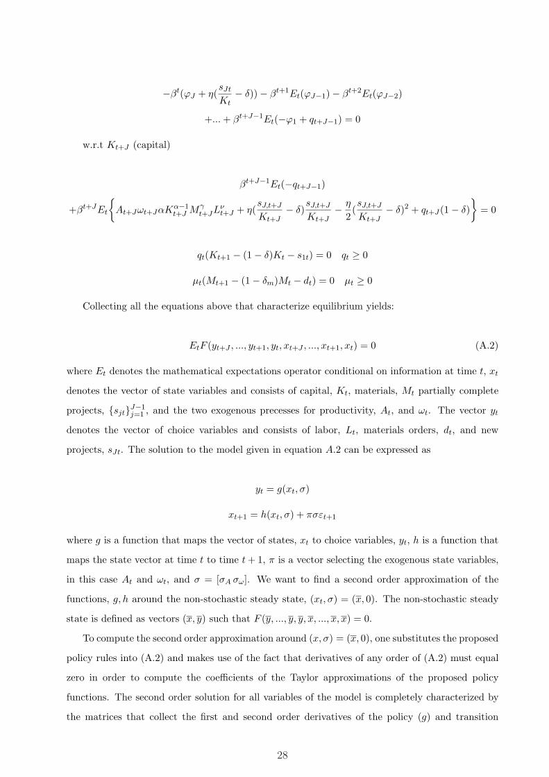
−βt(ϕJ + η(sJt

Kt− δ))− βt+1Et(ϕJ−1)− βt+2Et(ϕJ−2)

+... + βt+J−1Et(−ϕ1 + qt+J−1) = 0

w.r.t Kt+J (capital)

βt+J−1Et(−qt+J−1)

+βt+JEt

{At+Jωt+JαKα−1

t+J Mγt+JLν

t+J + η(sJ,t+J

Kt+J− δ)

sJ,t+J

Kt+J− η

2(sJ,t+J

Kt+J− δ)2 + qt+J(1− δ)

}= 0

qt(Kt+1 − (1− δ)Kt − s1t) = 0 qt ≥ 0

µt(Mt+1 − (1− δm)Mt − dt) = 0 µt ≥ 0

Collecting all the equations above that characterize equilibrium yields:

EtF (yt+J , ..., yt+1, yt, xt+J , ..., xt+1, xt) = 0 (A.2)

where Et denotes the mathematical expectations operator conditional on information at time t, xt

denotes the vector of state variables and consists of capital, Kt, materials, Mt partially complete

projects, {sjt}J−1j=1 , and the two exogenous precesses for productivity, At, and ωt. The vector yt

denotes the vector of choice variables and consists of labor, Lt, materials orders, dt, and new

projects, sJt. The solution to the model given in equation A.2 can be expressed as

yt = g(xt, σ)

xt+1 = h(xt, σ) + πσεt+1

where g is a function that maps the vector of states, xt to choice variables, yt, h is a function that

maps the state vector at time t to time t + 1, π is a vector selecting the exogenous state variables,

in this case At and ωt, and σ = [σA σω]. We want to find a second order approximation of the

functions, g, h around the non-stochastic steady state, (xt, σ) = (x, 0). The non-stochastic steady

state is defined as vectors (x, y) such that F (y, ..., y, y, x, ..., x, x) = 0.

To compute the second order approximation around (x, σ) = (x, 0), one substitutes the proposed

policy rules into (A.2) and makes use of the fact that derivatives of any order of (A.2) must equal

zero in order to compute the coefficients of the Taylor approximations of the proposed policy

functions. The second order solution for all variables of the model is completely characterized by

the matrices that collect the first and second order derivatives of the policy (g) and transition

28

(h) functions with respect to the state variables and σ, gx, hx, gxx, hxx, gσσ, hσσ. For example, the

second order approximation for g and h can be written respectively as (see Schmitt-Grohe and

Uribe (2004)),

[g(x, σ)]i = [g(x, 0)]i + [gx(x, 0)]ia(x− x)a +12[gxx(x, 0)]iab(x− x)a(x− x)b +

12[gσσ(x, 0)]i[σ][σ]

[h(x, σ)]j = [h(x, 0)]j + [hx(x, 0)]ja(x− x)a +12[hxx(x, 0)]jab(x− x)a(x− x)b +

12[gσσ(x, 0)]j [σ][σ]

where i = L, sJ , d, a, b = K, M, {sj}J−1j=1 , A, ω, j = K, M, {sj}J−1

j=1 , A, ω. [gx]ia, [hx]ia denote the

(i, a) element of the first order derivative of g, h with respect to x and similarly for the second

order derivatives. Notice that all the matrices collecting first and second order derivatives above are

evaluated at the non-stochastic steady state, i.e. (x, 0). In turn the non-stochastic steady state can

be easily computed by solving the f.o.c’s setting At = At+1 = E(A) and similarly ωt = ωt+1 = E(ω)

and solving the resulting static system of equations for x, y.

B Appendix 2

Time Aggregation. Derivation of equation 4.5. We begin with equation,

−4− η

( 4∑

k=1

(It,k

Kt,k− δ)

)+

4∑

k=1

qt,k = 0

where t denotes years.

If we add and subtract η

( ∑4k=1(

It,k

Kat− δ)

)we get

−4− η

( 4∑

k=1

(It,k

Kat

− δ))

+ η

(1

Kat

4∑

k=1

It,k

Kt,kKt,k −

4∑

k=1

It,k

Kt,k

)+

4∑

k=1

qt,k = 0

The term,(

1Ka

t

∑4k=1

It,k

Kt,kKt,k −

∑4k=1

It,k

Kt,k

)which will be 6= 0 in general, represents the time

aggregation error. It is easy to see that this term will be zero only when investment is equal to

replacement investment (δK), so that capital in year t, Kat = Kt,k. Similar expressions for the time

aggregation error characterize J = 2, 3, 4.

Re-writing this equation (dividing by four and using∑4

k=1It,k

Kat

= Iat

Kat, qa

t =∑4

k=1 qt,k

4 , 1η4

= 1ηa )

after suppressing all the constant terms yields equation 4.5 in the text,

Iat

Kat

= constant +(

1Ka

t

4∑

k=1

It,k

Kt,kKt,k −

4∑

k=1

It,k

Kt,k

)+

1ηa

qat

29

Alternative adjustment cost formulation. We now derive the Euler equation for new

projects, sJt, that corresponds to the following adjustment cost formulation,

G(s1,jt, ...sJ,jt,Kjt) =J∑

i=1

ϕiη

2(si,jt

Kjt− δ)2Kjt

This is given by,

−βt(ϕJ +ηϕJ(sJt

Kt−δ))−βt+1Et(ϕJ−1 +ηϕJ−1(

sJt

Kt+J−3−δ))−βt+2Et(ϕJ−2 +ηϕJ−2(

sJt

Kt+J−2−δ))

+... + βt+J−1Et − (ϕ1 + ηϕ1(sJt

Kt+J−1− δ)) + βt+J−1Etqt+J−1 = 0

The investment-q equation (using (2.3)) that this FOC implies for (J = 3) is given by,

Ij,t

Kj,t= ϕ3

(− 1

η(ϕ3 + βϕ2 + β2ϕ1) + δ(ϕ3 + βϕ2 + β2ϕ1)

)(ϕ3 + βϕ2g

−1kt+1

+ β2ϕ1g−1kt+1

g−1kt+2

)−1

+ϕ31ηβ2Et(qj,t+2)

(ϕ3 + βϕ2g

−1kt+1

+ β2ϕ1g−1kt+1

g−1kt+2

)−1

+2∑

i=1

ϕisi,jt

Kj,t

where gkt+1 = Kt+1

Kt, gkt+2 = Kt+2

Kt+1denote the growth rates of capital in t+1 and t+2 respectively.

This is similar to the baseline adjustment cost assumption investment-q equation. Importantly,

the implications from the omission of the RHS variable (∑2

i=1 ϕisi,jt

Kj,t) are very similar to those

implied by Table 3, i.e. there is also a cash-flow effect. Table 3B below summarizes the regression

results from this specification (using annual measures as in Table 3).

Empirical proxy. Next, we show the derivation of the empirical proxy in equation 4.7.

4∑

k=1

∑2i=1 ϕisit,k

Kt,k=

4∑

k=1

(It−1,k

Kt,k− ϕ1(1− (1− δ)

gt,k) + ϕ1(

ϕ2

ϕ1− 1)

s1t,k

Kt,k+ ϕ2(

ϕ3

ϕ2− 1)

s2t,k

Kt,k

)

The RHS of the equation above yields,

Iat−1

Kat

+4∑

k=1

(It−1,k

Kt,k− It−1,k

Kat

)− ϕ1

4∑

k=1

(1− (1− δ)

gt,k))

+(ϕ1(

ϕ2

ϕ1− 1)

s1t,k

Kt,k+ ϕ2(

ϕ3

ϕ2− 1)

s2t,k

Kt,k

)

Equation 4.7 in the text follows from the above when we impose the symmetry assumption of

TTB (i.e. ϕ1 = ϕ2 = ϕ3) and use gt,k u 14ga

t .

Coefficient bias. We derive the expressions that determine the biases in the coefficients of q

and the profit rate in the investment regression.

Consider the regression

30

y = X1β1 + X2β2 + X3β3 + u

where y = Iat

Kat, X1 = qa

t , X2 = πat

Kat, X3 =

∑4k=1

∑2i=1 ϕisit,k

Kt,k. The true coefficient of πa

tKa

twill be β2 = 0.

Now suppose we specify the following regression equation (i.e. equation 4.4)

y = X1β1 + X2β2 + e

where the error e term is now given by

e = X3β3 + u

The OLS coefficient vector is given by,

[b1

b2

]=

[X ′

1X1 X ′1X2

X ′2X1 X ′

2X2

][X ′

1y

X ′2y

]

Using standard matrix formulas this equation can be written as,

[b1

b2

]=

[D−1

1 D−12

D−13 D−1

4

][X ′

1y

X ′2y

]

where D−11 = (X ′

1X1 −X ′1X2(X ′

2X2)−1X ′2X1)−1,

D−12 = −(X ′

1X1 −X ′1X2(X ′

2X2)−1X ′2X1)−1(X ′

1X2)(X ′2X2)−1,

D−13 = −(X ′

2X2)−1(X ′2X1)(X ′

1X1 −X ′1X2(X ′

2X2)−1X ′2X1)−1,

D−14 = (X ′

2X2)−1 + (X ′2X2)−1(X ′

2X1)(X ′1X1 −X ′

1X2(X ′2X2)−1X ′

2X1)−1(X ′1X2)(X ′

2X2)−1

The expected value of the OLS coefficients on the profit rate and marginal q will be given by,

E(b2) = [D−13 (X ′

1X1) + D−14 (X ′

2X1)]β1 + [D−13 (X ′

1X3) + D−14 (X ′

2X3)]β3

E(b1) = [D−11 (X ′

1X1) + D−12 (X ′

2X1)]β1 + [D−11 (X ′

1X3) + D−12 (X ′

2X3)]β3

One can show that D−11 > 0, D−1

2 < 0, D−13 < 0, D−1

4 > 0 as long as (X ′1X1−X ′

1X2(X ′2X2)−1X ′

2X1)−1 >

0. Since X1 = qat , X2 = πa

tKa

tthis condition simplifies to (var(qa

t )−cov(qat ,

πat

Kat)var( πa

tKa

t)−1cov(qa

t ,πa

tKa

t)) >

0. This can further be written as 1 > ρ2x1,x2

which will be always satisfied unless ρ2x1,x2

= 1. It is

easy to see from the expressions above that when this condition is satisfied, E(b2) will rise with β3,

while E(b1) will fall with β3. Therefore as long as ϕJ is falling with J this will always be the case.

31

Table 1

Calibrated parameters (baseline)

Technology

γ=0.53

ν = 0.32

α=0.13

Investment

ϕ1=0.33

ϕ2=0.34

ϕ3=0.33

Depreciation

δ=0.025

δm=0.75

Discount factor

β = 11+r

= 0.99

Adjustment cost parameter

ηa=0.27 (Barnett and Sakellaris (1999))

Productivity process (common)

σA=0.045 ρA = 0.9

Productivity process (idiosyncratic)

σω=0.025 ρω = 0.9

Table 2

Investment regressions: empirical specification

Quarterly model

Coefficient J = 1 J = 2 J = 3 J = 4

b1 0.91 0.55 0.41 0.33

(0.0001) (0.001) (0.002) (0.002)

b2 0.0001 0.49 0.54 0.58

(0.0001) (0.001) (0.002) (0.003)

R2

0.99 0.97 0.92 0.87

Notes. The Table reports coefficients of the regression,Ij,t

Kj,t= α + b1Et(qj,t+2) + b2

πj,t

Kj,t+ εj,t. Standard errors are in

parenthesis. All statistics are averages over 500 replications.

32

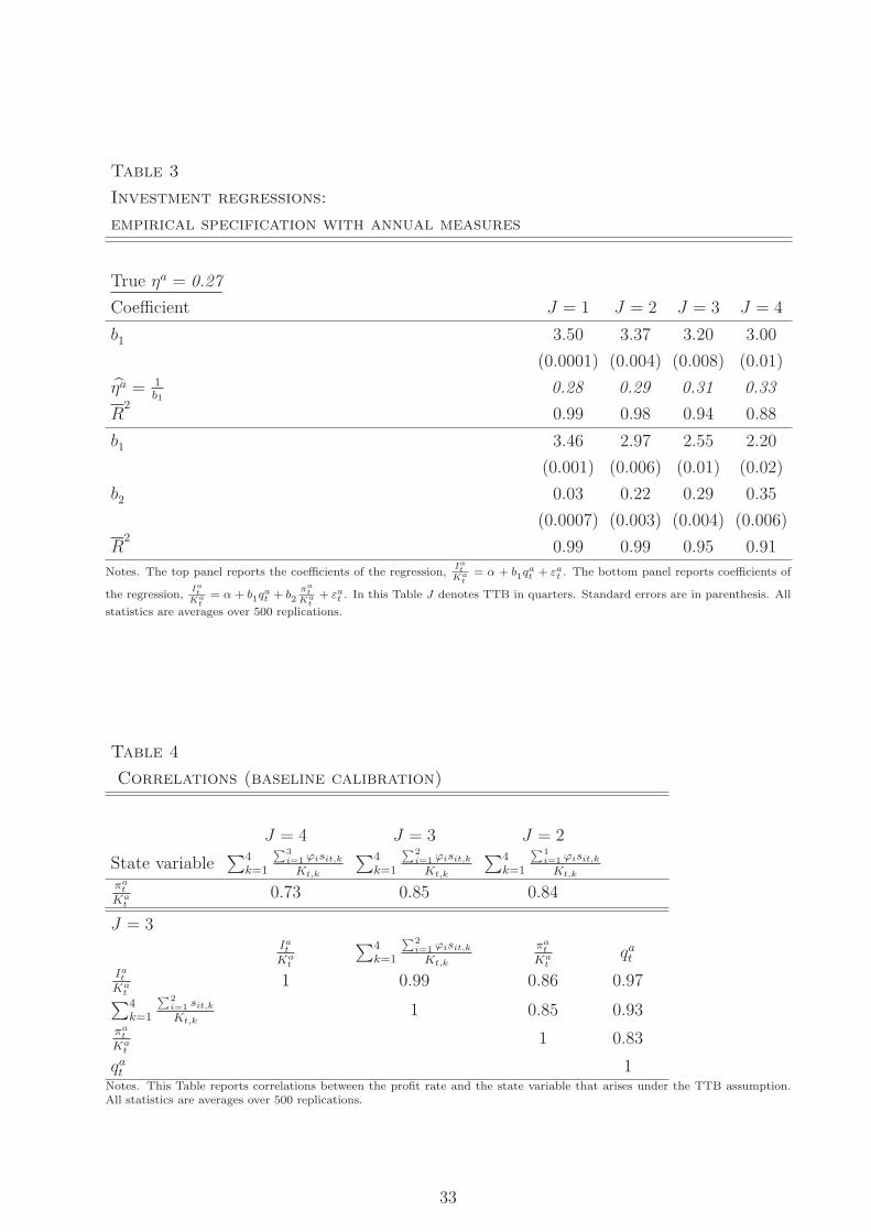
Table 3

Investment regressions:

empirical specification with annual measures

True ηa = 0.27

Coefficient J = 1 J = 2 J = 3 J = 4

b1 3.50 3.37 3.20 3.00

(0.0001) (0.004) (0.008) (0.01)

η̂a = 1b1

0.28 0.29 0.31 0.33

R2

0.99 0.98 0.94 0.88

b1 3.46 2.97 2.55 2.20

(0.001) (0.006) (0.01) (0.02)

b2 0.03 0.22 0.29 0.35

(0.0007) (0.003) (0.004) (0.006)

R2

0.99 0.99 0.95 0.91

Notes. The top panel reports the coefficients of the regression,Iat

Kat

= α + b1qat + εa

t . The bottom panel reports coefficients of

the regression,Iat

Kat

= α + b1qat + b2

πat

Kat

+ εat . In this Table J denotes TTB in quarters. Standard errors are in parenthesis. All

statistics are averages over 500 replications.

Table 4

Correlations (baseline calibration)

J = 4 J = 3 J = 2

State variable∑4

k=1

∑3i=1 ϕisit,k

Kt,k

∑4k=1

∑2i=1 ϕisit,k

Kt,k

∑4k=1

∑1i=1 ϕisit,k

Kt,k

πat

Kat

0.73 0.85 0.84

J = 3Iat

Kat

∑4k=1

∑2i=1 ϕisit,k

Kt,k

πat

Kat

qat

Iat

Kat

1 0.99 0.86 0.97∑4

k=1

∑2i=1 sit,k

Kt,k1 0.85 0.93

πat

Kat

1 0.83

qat 1

Notes. This Table reports correlations between the profit rate and the state variable that arises under the TTB assumption.All statistics are averages over 500 replications.

33

Table 5

Investment regressions:

time-to-plan

True ηa = 0.27

Coefficient J = 2 J = 3 J = 4

b1 3.34 3.19 2.92

(0.009) (0.01) (0.01)

η̂a = 1b1

0.30 0.31 0.34

R2

0.93 0.86 0.75

b1 2.70 2.35 1.75

(0.01) (0.01) (0.002)

b2 0.44 0.45 0.50

(0.006) (0.007) (0.01)

R2

0.95 0.89 0.80

Notes. The top panel reports the coefficients of the regression,Iat

Kat

= α + b1qat + εa

t . The bottom panel reports coefficients of

the regression,Iat

Kat

= α + b1qat + b2

πat

Kat

+ εat . In this Table J denotes TTB in quarters. Standard errors are in parenthesis. All

statistics are averages over 500 replications.

Table 6

Investment regressions:

empirical specification with annual measures and

proxy for state variable

True ηa = 0.27

Coefficient J = 2 J = 3 J = 4

b1 3.63 3.62 3.67

(0.0006) (0.0003) (0.0002)

η̂a = 1b1

0.27 0.27 0.27

R2

0.99 0.99 0.99

b1 3.68 3.69 3.80

(0.003) (0.002) (0.002)

b2 0.03 0.03 0.02

(0.0008) (0.0008) (0.0006)

b3 0.89 0.91 0.93

(0.002) (0.001) (0.0008)

R2

0.99 0.99 0.99

Notes. The top panel reports the coefficients of the regression,Iat

Kat

= α + b1qat + b3(

Iat−1Ka

t− 4ϕ1(1− 4(1−δ)

gat

)) + εat . The bottom

panel reports coefficients of the regression,Iat

Kat

= α + b1qat + b2

πat

Kat

+ b3(Iat−1Ka

t− 4ϕ1(1− 4(1−δ)

gat

)) + εat . In the top panel only

coefficient b1 is reported. In this Table J denotes TTB in quarters. Standard errors are in parenthesis. All statistics areaverages over 500 replications.

34

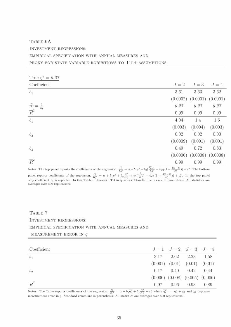
Table 6A

Investment regressions:

empirical specification with annual measures and

proxy for state variable-robustness to TTB assumptions

True ηa = 0.27

Coefficient J = 2 J = 3 J = 4

b1 3.61 3.63 3.62

(0.0002) (0.0001) (0.0001)

η̂a = 1b1

0.27 0.27 0.27

R2

0.99 0.99 0.99

b1 4.04 1.4 1.6

(0.003) (0.004) (0.003)

b2 0.02 0.02 0.00

(0.0009) (0.001) (0.001)

b3 0.49 0.72 0.83

(0.0006) (0.0008) (0.0008)

R2

0.99 0.99 0.99

Notes. The top panel reports the coefficients of the regression,Iat

Kat

= α + b1qat + b3(

Iat−1Ka

t− 4ϕ1(1− 4(1−δ)

gat

)) + εat . The bottom

panel reports coefficients of the regression,Iat

Kat

= α + b1qat + b2

πat

Kat

+ b3(Iat−1Ka

t− 4ϕ1(1 − 4(1−δ)

gat

)) + εat . In the top panel

only coefficient b1 is reported. In this Table J denotes TTB in quarters. Standard errors are in parenthesis. All statistics areaverages over 500 replications.

Table 7

Investment regressions:

empirical specification with annual measures and

measurement error in q

Coefficient J = 1 J = 2 J = 3 J = 4

b1 3.17 2.62 2.23 1.58

(0.001) (0.01) (0.01) (0.01)

b2 0.17 0.40 0.42 0.44

(0.006) (0.008) (0.005) (0.006)

R2

0.97 0.96 0.93 0.89

Notes. The Table reports coefficients of the regression,Iat

Kat

= α + b1qat + b2

πat

Kat

+ εat where qa

t == qat + χt and χt captures

measurement error in q. Standard errors are in parenthesis. All statistics are averages over 500 replications.

35

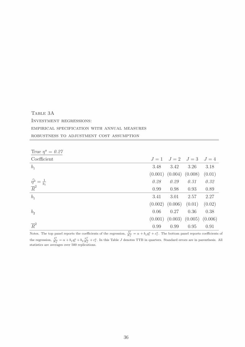
Table 3A

Investment regressions:

empirical specification with annual measures

robustness to adjustment cost assumption

True ηa = 0.27

Coefficient J = 1 J = 2 J = 3 J = 4

b1 3.48 3.42 3.26 3.18

(0.001) (0.004) (0.008) (0.01)

η̂a = 1b1

0.28 0.29 0.31 0.32

R2

0.99 0.98 0.93 0.89

b1 3.41 3.01 2.57 2.27

(0.002) (0.006) (0.01) (0.02)

b2 0.06 0.27 0.36 0.38

(0.001) (0.003) (0.005) (0.006)

R2

0.99 0.99 0.95 0.91

Notes. The top panel reports the coefficients of the regression,Iat

Kat

= α + b1qat + εa

t . The bottom panel reports coefficients of

the regression,Iat

Kat

= α + b1qat + b2

πat

Kat

+ εat . In this Table J denotes TTB in quarters. Standard errors are in parenthesis. All

statistics are averages over 500 replications.

36

Working Paper List 2008

Number Author Title

08/10 Marta Aloi, Manuel Leite-Monteiro and Teresa Lloyd-Braga

Unionized Labor Markets and Globalized Capital Markets

08/09 Simona Mateut, Spiros Bougheas and Paul Mizen

Corporate trade credit and inventories: New evidence of a tradeoff from accounts payable and receivable

08/08 Christos Koulovatianos, Leonard J. Mirman and Marc Santugini

Optimal Growth and Uncertainty: Learning

08/07 Christos Koulovatianos, Carsten Schröder and Ulrich Schmidt

Nonmarket Household Time and the Cost of Children

08/06 Christiane Baumeister, Eveline Durinck and Gert Peersman

Liquidity, Inflation and Asset Prices in a Time-Varying Framework for the Euro Area

08/05 Sophia Mueller-Spahn The Pass Through From Market Interest Rates to Retail Bank Rates in Germany

08/04 Maria Garcia-Vega and Alessandra Guariglia

Volatility, Financial Constraints and Trade

08/03 Richard Disney and John Gathergood

Housing Wealth, Liquidity Constraints and Self-Employment

08/02 Paul Mizen and Serafeim Tsoukas What Effect has Bond Market Development in Asia had on the Issue of Corporate Bonds

08/01 Paul Mizen and Serafeim Tsoukas Modelling the Persistence of Credit Ratings When Firms Face Financial Constraints, Recessions and Credit Crunches

Working Paper List 2007

Number Author Title

07/11 Rob Carpenter and Alessandra Guariglia

Investment Behaviour, Observable Expectations, and Internal Funds: a comments on Cummins et al, AER (2006)

07/10 John Tsoukalas The Cyclical Dynamics of Investment: The Role of Financing and Irreversibility Constraints

07/09 Spiros Bougheas, Paul Mizen and Cihan Yalcin

An Open Economy Model of the Credit Channel Applied to Four Asian Economies

07/08 Paul Mizen & Kevin Lee Household Credit and Probability Forecasts of Financial Distress in the United Kingdom

07/07 Tae-Hwan Kim, Paul Mizen & Alan Thanaset

Predicting Directional Changes in Interest Rates: Gains from Using Information from Monetary Indicators

07/06 Tae-Hwan Kim, and Paul Mizen Estimating Monetary Reaction Functions at Near Zero Interest Rates: An Example Using Japanese Data

07/05 Paul Mizen, Tae-Hwan Kim and Alan Thanaset

Evaluating the Taylor Principle Over the Distribution of the Interest Rate: Evidence from the US, UK & Japan

07/04 Tae-Hwan Kim, Paul Mizen and Alan Thanaset

Forecasting Changes in UK Interest rates

07/03 Alessandra Guariglia Internal Financial Constraints, External Financial Constraints, and Investment Choice: Evidence From a Panel of UK Firms

07/02 Richard Disney Household Saving Rates and the Design of Public Pension Programmes: Cross-Country Evidence

07/01 Richard Disney, Carl Emmerson and Matthew Wakefield

Public Provision and Retirement Saving: Lessons from the U.K.

Working Paper List 2006

Number Author Title

06/04 Paul Mizen & Serafeim Tsoukas Evidence on the External Finance Premium from the US and Emerging Asian Corporate Bond Markets

06/03 Woojin Chung, Richard Disney, Carl Emmerson & Matthew Wakefield

Public Policy and Retirement Saving Incentives in the U.K.

06/02 Sarah Bridges & Richard Disney Debt and Depression

06/01 Sarah Bridges, Richard Disney & John Gathergood

Housing Wealth and Household Indebtedness: Is There a 'Household Financial Accelerator'?

Working Paper List 2005

Number Author Title

05/02 Simona Mateut and Alessandra Guariglia

Credit channel, trade credit channel, and inventory investment: evidence from a panel of UK firms

05/01 Simona Mateut, Spiros Bougheas and Paul Mizen

Trade Credit, Bank Lending and Monetary Policy Transmission