cfd analysis and design optimization of flapping wing ... · kunigal shivakumar co-advisor sanjiv...

CFD Analysis and Design Optimization of Flapping Wing Flows

Martin Alexander Jones

North Carolina A&T State University

A dissertation submitted to the graduate faculty

in partial fulfillment of the requirements for the degree of

DOCTOR OF PHILOSOPHY

Department: Mechanical Engineering

Major: Mechanical Engineering

Co-Advisor: Dr. Kunigal Shivakumar

Co-Advisor: Dr. Nail Yamaleev

Greensboro, North Carolina

2013

i

School of Graduate Studies

North Carolina Agricultural and Technical State University

This is to certify that the Doctoral Dissertation of


has met the dissertation requirements of

North Carolina Agricultural and Technical State University

Greensboro, North Carolina

2013

Approved by:

Kunigal Shivakumar

Co-Advisor

Sanjiv Sarin

Dean, The Graduate School

Nail Yamaleev

Co-Advisor

Eric Nielsen

Committee Member

Sanjiv Sarin

Dean, The Graduate School

Samuel Owusu-Ofori

Department Chair

Arturo Fernandez

Committee Member

Julius Harp

Graduate School Representative

ii

© Copyright by


2013

iii

Biographical Sketch

Martin Jones received his B.S. in Physics with a minor in Mathematics and a M.S. in

Nuclear Physics from North Carolina A&T State University in the summer of 2007 and 2009,

respectively. This work concludes efforts towards a Ph.D. degree in Mechanical Engineering at

NC A&T State University on Computational Fluid Dynamics (CFD) analysis and Design

Optimization of flapping-wing flows that occur at low Reynolds numbers using CFD. He has

performed CFD analysis and design optimization of unsteady turbulent flows using Fully

Unstructured Navier – Stokes 3D (FUN3D) solver developed by NASA Langley Research

Center.

To highlight some of his research, in 2006, he was awarded a summer fellowship from

the Leadership Alliance to work with Professors Callan and Bialek at Princeton University.

There he learned about techniques in Computational Biology and Biophysics to discover binding

sites of proteins in what was thought to be the “junk DNA” regions of the genome of several

yeast species in the Saccharomyces genus. During his tenure as a masters graduate student, he

did much of his work at Thomas Jefferson National Laboratory where he helped build, install,

and do analysis on one detector in a complex of electronic and particle detection equipment for

the SANE (Spin Asymmetries on the Nucleon Experiment) experiment in Hall – C at JLab. In

the summer of 2011, he did a sojourn at NASA Langley Research Center in Hampton, VA.

There he did CFD analysis on a UAV (Unmanned Aerial Vehicle) called KAHU as a part of the

Configuration Aerodynamics Branch under the tutelage of Sally Viken.

He was invited by his current advisor, Dr. Nail Yamaleev, to study CFD in 2009. This

experience has added to his understanding of numerical methods greatly.

iv

Dedication

To my Father, Counselor, and Comforter

+ To my parents

+ To my mentors

_________________________________

=

v

Acknowledgements

This is for all the teachers in my life. To my Mother, Father, and Sister: So many lessons

I’ve learned, you taught me to seek greatness, and to love God. I attribute almost everything I am

to you guys, thanks. Never to forget my extended family: my Grandparents, of who I remember

teaching me being Grandma Jones and Mommybee: thanks to you!

For the teachers in my later years: A few of you have stood out from public school,

especially my violin teacher, Ms. Barbee. I’m sad you couldn’t teach us just a few more years

until I graduated from high school. And the man that showed us a Physics video that changed my

life forever, also my swim coach!: Coach Griffin.

And to the teachers in my undergraduate years: All the experiences I had in all that I went

through, thanks to Dr. Bililign, for broadening my horizons, Dr. Danagoulian and his wife, you

have both touched my heart, Dr. Sandin (Maybe one day my family will have a Jones Para-

docs!), Dr. James, just for you and your wonderful style, Dr. Gasparian, for your seriousness

regarding dedication to physics, Dr. Kebede, thanks for the talks, Doc Lock, thanks for the

camaraderie, my thesis advisor, Dr. Ahmidouch, for your kindness, and Dr. Levy, for

heartwarming dedication to my well-being.

And to my graduate teachers: My Doctoral Committee, Dr. Shivakumar, Dr. Yamaleev,

Dr. Nielsen, and Dr. Fernandez, thank you for all your guidance and presence on the committee.

To my other doctoral teachers: Dr. Sundaresan, Dr. Kabadi, Dr. Kizito, Dr. Antonio, Dr.

Ferguson, for your support and experience during my stay.

To my formal mentors: Dr. Shivakumar and Dr. Yamaleev, both of your guidance and

understanding have known no bounds, and it has been my pleasure working with you in the

vi

student/mentor capacity to transfer confidence, respect, and friendship. I look forward to future

collaboration in the future.

And to my informal mentors: It was my dream to be like the famous physicists of old and

live a life of discovery like them. I have that now. (Or it’s a process.)

I spent a lot of time learning physics and math from you, Bob. My time spent with you

was precious. You saw me wake up into enlightenment, and you taught me how to listen, like

you said, a major problem with our culture today. I knew you like a Grandpa, one that I never

had as an adult. You are famous in your own right and are a true American scholar.

And to my mentor: Dr. Levy (And Dr. Michelle!). I was so enthusiastic about taking your

Physics class that first time around and somehow that grew into a lasting relationship because I

guess we both love solving problems so much, even if we sometimes want to solve problems like

the minimum number of times it takes to weigh 50 doughnuts with a scale balance when one

weighs less than the others! I haven’t figured that one out yet. You have helped me when I was at

my worst, going far beyond the duties of just an ordinary teacher. You let me work with you on a

problem for my very first paper. I have received more than I could ever have imagined from you

and Academia and I look forward to the future.

I also don’t want to forget the NASA CAS and CCMR staff and student colleagues for all

your encouragement and help.

I love all of you and wish the best on you all. Thanks.

Martin A. Jones

vii

Table of Contents

List of Figures .............................................................................................................................x

List of Tables .......................................................................................................................... xiii

Key to Symbols or Abbreviations .............................................................................................xiv

Abstract ......................................................................................................................................2

CHAPTER 1 Introduction ...........................................................................................................3

1.1 Unsteady Physics Mechanisms Involved in Insect Flight ....................................................4

1.1.1 Insect flight kinematics. .................................................................................................5

1.1.2 Unsteady Mechanisms. ...................................................................................................7

1.2 Model Selection. ................................................................................................................9

1.3 Objectives of the Research ............................................................................................... 10

1.4 Scope of the Dissertation ................................................................................................. 10

1.5 Philosophy Used in this Dissertation ................................................................................ 11

CHAPTER 2 Governing Navier-Stokes Equations and Numerical Scheme................................ 14

2.1 Introduction and Theory................................................................................................... 14

2.2 Second-Order Node-Centered Finite Volume Scheme ...................................................... 16

2.3 Moving Grids .................................................................................................................. 17

2.4 Geometric Conservation Law (GCL). .............................................................................. 18

2.5 Second-order Backward Difference (BDF2) Scheme ....................................................... 19

2.6 Spalart-Allmaras Turbulence Model ................................................................................ 20

2.7 Low-Mach Preconditioner ............................................................................................... 21

viii

CHAPTER 3 CFD Analysis of Flapping-Wing Flows ............................................................... 23

3.1 Introduction ..................................................................................................................... 23

3.1.1 Literature survey. ......................................................................................................... 23

3.1.2 Validation of FUN3D code........................................................................................... 26

3.2 Three-Dimensional Simulations ....................................................................................... 29

3.2.1 Wing kinematics. ......................................................................................................... 29

3.2.2 Computational grid....................................................................................................... 30

3.2.3 Grid refinement study. .................................................................................................. 31

3.2.4 Reynolds number sensitivity......................................................................................... 32

3.2.5 Simulation of gust pulse. .............................................................................................. 33

3.3 Results ............................................................................................................................. 34

3.3.1 Frontal gust. ................................................................................................................. 34

3.3.2 Downward gust. ........................................................................................................... 38

3.3.3 Side gust. ..................................................................................................................... 41

3.4 Discussion ....................................................................................................................... 46

CHAPTER 4 Adjoint-based Optimization of Flapping–Wing Flows ......................................... 50

4.1 Introduction ..................................................................................................................... 50

4.2 Governing Equations and Numerical Method ................................................................... 52

4.3 Wing Kinematics and Associated Design Variables ......................................................... 53

4.4 Shape Parameterization .................................................................................................... 54

ix

4.5 Time-Dependent Adjoint-Based Optimization Methodology ............................................ 57

4.6 Numerical Results ............................................................................................................ 59

4.7 Shape, Kinematics, and Shape/Kinematics Cases ............................................................. 62

4.7.1 Shape optimization. ...................................................................................................... 62

4.7.2 Kinematics optimization. .............................................................................................. 66

4.7.3 Combined Kinematics and Shape Optimization. ........................................................... 70

4.8 Validation of optimization results .................................................................................... 75

4.9 Discussion ....................................................................................................................... 76

CHAPTER 5 Concluding Remarks and Future Research ........................................................... 79

5.1 Concluding Remarks ........................................................................................................ 79

5.1.1 Wind gust analysis. ...................................................................................................... 79

5.1.2 Adjoint-based optimization. ......................................................................................... 80

5.2 Future Research ............................................................................................................... 81

References ................................................................................................................................ 84

x

List of Figures

Figure 1.1. Diagram showing the typical definition of wing chord and span (Sane, 2003) ............5

Figure 1.2. Illustration of insect flight kinematics terms. .............................................................6

Figure 2.1. An example of control volume around a node (0). ................................................... 17

Figure 3.1. Comparison of the lift (left) and drag coefficients obtained with the FUN3D code and

the numerical results of Yuan et al. and Malhan et al. ................................................................ 27

Figure 3.2. Comparison of pressure coefficient contours computed using the FUN3D code (left

column) with the CFD results of Yuan et al. .............................................................................. 28

Figure 3.3. Diagram labeling wing position at fractions of the period of one whole stroke. ........ 30

Figure 3.4. Hexahedral grid around the Robofly wing. .............................................................. 30

Figure 3.5. Thrust coefficient obtained on coarse, medium, and fine grids ................................. 31

Figure 3.6. Lift (left) and drag coefficients for the Robofly wing at Re=300, 4800, 16000. ........ 32

Figure 3.7. The ratio of the mean lift to the mean drag versus Reynolds number........................ 33

Figure 3.8. Time histories of the gust velocity and the wing thrust coefficient computed with and

without the frontal gust.............................................................................................................. 36

Figure 3.9. Cycle-averaged (over one full stroke) thrust coefficient for the frontal gust case. ..... 36

Figure 3.10. Snapshots of the iso-surface of the q-criterion colored with pressure contours at four

instants in time: (a-b) t=3500, (c-d) t=3600, (e-f) t=4000, (g-h) t=4100, obtained with (right

column) and without frontal gust. .............................................................................................. 37

Figure 3.11. Time histories of the gust velocity and the wing thrust coefficient computed with

and without downward gust. ...................................................................................................... 39

Figure 3.12. Cycle-averaged (over one full stroke) thrust coefficient for the downward gust case.

................................................................................................................................................. 39

xi

Figure 3.13. Snapshots of iso-surface of the q-criterion colored with pressure contours at four

instants in time(a-b) t=3500, (c-d) t=3600, (e-f) t=4000, (g-h) t=4100, obtained with (right

column) and without downward gust. ........................................................................................ 40

Figure 3.14. Time histories of the wind gust velocity and the thrust coefficient of a flapping wing

with and without root-to-tip side gust. ....................................................................................... 42


instants in time (a-b) t=3500, (c-d) t=3600, (e-f) t=4000, (g-h) t=4100, obtained with (right

column) and without root-to-tip side gust. ................................................................................. 43

Figure 3.16. Thrust response of the wing in a tip-to-root gust. ................................................... 46



column) and without tip-to-root side gust. ................................................................................. 45

Figure 3.18. Cycle-averaged (over one full stroke) thrust coefficient for the side gust case. ....... 46

Figure 3.19. A bee maneuvering in a side gust. .......................................................................... 48

Figure 4.1. Wing surface meshes generated by MASSOUD at baseline, medium, and large values

of design variable 13 that controls the wing span and aspect ratio. ............................................. 55

Figure 4.2. Wing surface meshes generated by MASSOUD at baseline, medium, and large values

by varying design variable 28 that controls the twist. ................................................................. 56

Figure 4.3. Convergence history of the objective functional for the first test problem. ............... 63

Figure 4.4. Planform and cross section of the wing before and after optimization. .................... 63

Figure 4.5. Iso-surface of the q-criterion colored with pressure contours at phase angles

obtained for the baseline (left column) and optimized wing

geometry. .................................................................................................................................. 64

xii

Figure 4.6. (a) Baseline and optimal thrust profiles. (b) Propulsive efficiency before and after

shape optimization. ................................................................................................................... 65

Figure 4.7. (a) Convergence history of the objective functional. (b) Baseline and optimal stroke,

pitch, and heave angles. ............................................................................................................. 66

Figure 4.8. Iso-surface of the q-criterion colored with pressure contours at phase angles

obtained for the baseline (left column) and optimized wing

kinematics. ................................................................................................................................ 68


optimization. ............................................................................................................................. 69


pitch, and heave angles. ............................................................................................................. 71

Figure 4.11. Planforms (left) and cross sections (right) of the wing before and after combined

optimization of the wing shape and kinematics. ......................................................................... 71

Figure 4.12. Iso-surface of the q-criterion at phase angles

obtained for the baseline (left column) and optimized wing kinematics and geometry. .............. 72


optimization of wing shape and kinematics. .............................................................................. 73

Figure 4.14. Stroke-averaged thrust and propulsive efficiency of the baseline and optimized

configurations. .......................................................................................................................... 75

Figure 4.15. Thrust coefficient (a) and propulsive efficiency computed on the baseline and fine

grids .......................................................................................................................................... 75

xiii

List of Tables

Table 1 The range of insect, MAV, and NAV Reynolds numbers. ...............................................5

xiv

Key to Symbols or Abbreviations

x,y,z………………..Spatial coordinates

t…………………….Time (always non-dimensional unless otherwise stated)

τ…………………….Pseudo-Time

COG……………….Center of Gravity

Q…………………...Vector of Conservative Variables

D…………………...Vector of Design Variables

Fi………………….. Inviscid flux vector

Fv…………………..Viscous flux vector

………….Periodic Splines

θ……………………Stroke Angle

α……………………Pitching Angle

φ……………………Heaving Angle

k……………………Reduced frequency

V…………………...Volume

Γ……………………Control Volume Around Individual Nodes

W…………………...Local Face Velocity Vector

…………………...The Normal Vector to the Side When Evaluating Fluxes

T…………………… Transformation Matrix

T…………………….Period

m……………………Pseudo-time Counter

n…………………….Real-time Counter

P…………………….Preconditioning Matrix

xv

…………………..Vector of Flow Lagrange Multipliers

…………………..Vector of Grid Lagrange Multipliers

θcn, θsn....................... Fourier-like amplitudes

E …………………...Energy

ρ …………………...density

u,v,w ………………x,y,z components of the velocity

p …………………...pressure

Wi …………………x,y,z components of the local face velocity vector

i,j,k ………………..x,y,z, unit vectors

P ………………….. Preconditioning Matrix

q-criterion …………A qualitative measure of vorticity in the flow field

2

Abstract

The main objectives of this research work are to perform the CFD analysis of the 3-D flow

around a flapping wing in a gusty environment and to optimize its kinematics and shape to

maximize the performance. The effects of frontal, side, and downward wind gusts on the

aerodynamic characteristics of a rigid wing undergoing insect-based flapping motion are

analyzed numerically. The turbulent, low-Reynolds-number flow near a flapping wing is

governed by the 3-D unsteady Reynolds-Averaged Navier-Stokes (URANS) equations with the

Spalart-Allmaras turbulence model. The governing equations are solved using a second-order

node-centered finite volume method on a hexahedral mesh that rigidly moves along with the

wing. Our numerical results show that a centimeter-scale wing considered is susceptible to strong

downward wind gusts. In the case of frontal and side gusts, the flapping wing can alleviate the

gust effect if the gust velocity is less than or comparable to the wing tip velocity. The second

objective is to optimize the wing kinematics and shape to improve its aerodynamic

characteristics. To our knowledge, this is the first attempt to perform high-fidelity combined

optimization of flapping wing kinematics and shape in 3-D unsteady turbulent flows. For our

optimization studies, an adjoint-based gradient method using the method of Lagrange multipliers

is employed to minimize an objective functional with the 3D URANS and grid equations as

constraints. It has been shown that some unsteady phenomena such as the clap and fling

mechanism found in use by flying insects (e.g., a wasp Encarsaria formosa, or greenhouse

white-fly Trialeurodes vaporariorium), maximize the wing propulsive efficiency. These results

indicate that the time-dependent adjoint-based optimization method is an efficient tool for design

of a new generation of micro air vehicles.

3

CHAPTER 1

Introduction

Most flying insects are equipped with an exemplary aerodynamic propulsion system

rivaled by no known man-made system. An insect’s maneuverability, mobility, autonomy,

agility, and recoverability in seemingly impossible flight conditions obviously impress the

engineer from an aerodynamic standpoint. Lately, a strong effort has been made to manufacture

flying craft that have some of the flight characteristics, stealth, and maneuvering advantages of

biological flyers. Since the 19th

century there has been an interest in micro-sized man-made

flyers that eventually led to a controlled effort after the development of Unmanned Aerial

Vehicles (UAVs) to create Micro Air Vehicles (MAVs) that have a maximum dimension of 7.5

to 15 cm. Those with maximum dimension less than 7.5 cm DARPA classifies as a Nano Air

Vehicle (NAV). These robotic flyers can be used for military, scientific, and civil applications.

Some possible scientific applications include non-intrusive observation of animals in the wild,

even integration into natural swarms of living insects to study their behavior. Potential

recreational applications include flying toys for children or adults which can even lead to

educational tools for the STEM-inspired classrooms of tomorrow.

There are four common types of MAVs that have appeared in the literature. These are

fixed wing craft, rotary blade (helicopter-like and mill wheel-like), ornithopters, and flapping

wing MAVs. All but the flapping wing MAVs and mill wheel rotary blade type have larger

counterparts in the UAV family and even in the class of manned vehicles, the most obvious for

fixed wing and rotary wing being the commercial jet and military helicopter, respectively. This

fact is very important to note because it points out that we can reasonably expect and predict the

flight capabilities that these types of MAVs have. However, the aerodynamic characteristics of

4

flapping-wing MAVs are entirely different as compared with those of the conventional rotary- or

fixed-wing counterparts. To achieve the flight capabilities of biological flyers, it would be

extremely important to understand the fundamental flow physics underlying the relationships

between wing shape and kinematics and the aerodynamic response in varying flight conditions to

be encountered in the atmospheric boundary layer where the flapping wing MAV will be

expected to perform its function. The focus of the following dissertation is on the problem of

realizing more efficient flapping wing MAVs through optimization of kinematic and shape

parameters, using the adjoint-based methodology developed in (Nielsen & Anderson,

Aerodynamic Design Optimization on Unstructured Meshes Using the Navier-Stokes Equations,

1998) (Nielsen, Diskin, & Yamaleev, Discrete Adjoint-Based Design Optimization of Unsteady

Turbulent Flows on Dynamic Unstructured Grids, 2010). A minor secondary focus of this

research is to determine whether the kinematics and shape of wings found in extant species of

insects can be used as guidance for conceptual design of MAVs. Also we would like to observe

similar kinematic and shape features found in the insect world such as rapid wing rotations

during stroke reversals, significant deviation of the wing from the mean stroke plane, wing

profiles with high aspect ratio, etc., when an optimization is accomplished from a baseline shape

or kinematic design.

1.1 Unsteady Physics Mechanisms Involved in Insect Flight

It is helpful to analyze the aerodynamic characteristics of biological flyers because their

crucial non-dimensional quantities such as Strouhal number, reduced flapping frequency, and

Reynolds numbers (refer to Table 1) are very similar to those of the current and futuristic MAVs.

5

Table 1

The range of insect, MAV, and NAV Reynolds numbers.

Biological flyers Kinematic

Viscosity (m2/s)

Characteristic wing

length (m)

Characteristic

Speed (m/s)

Reynolds

Number

Fungus Gnat

1.33E-05

0.0025

0.42 79

0.63 119

1.00 188

Bumblebee

0.010

3.00 2,258

3.60 2,710

4.50 3,387

Ruby-Throated

Hummingbird 0.045

13.40 44,885

22.30 74,696

28.00 93,789

According to Sane, “using standard aerodynamic theory, insect flight appears

improbable” (Sane, 2003). Understanding the physics of insect flight will inevitably help to

understand how to design more efficient MAVs with some of the flight characteristics of

biological flyers. Figure 1.1 displaying key definitions for describing wings in insects and MAVs

follows:

Figure 1.1. Diagram showing the typical definition of wing chord and span (Sane, 2003)

1.1.1 Insect flight kinematics. A simple way to understand insect flight kinematics

would be to state: the way that the lifting surfaces (wings) move to produce thrust or specific

flight maneuvers (e.g., saccades’ sudden right- or left-angle turns). There are four main stages of

6

wing motion in typical insect flight, as shown in Fig. 2. The topology of the wing tip trajectory

projected onto the only symmetry plane of an insect (the solid line in Fig. 1.2) can vary and will

sometimes produce a figure-eight shape depending on the insect or type of maneuver that it

makes. Supination and pronation are two turning points where the wings make a rapid rotation in

pitch angle about the span-wise axis of the wing and the upstroke and downstroke are backward

and forward strokes, respectively. Important flow phenomena occur during each of these

distinctive parts of the flapping wing in motion. The physics of unsteady mechanisms that

account for the ability of the flying insect will be covered in Section 1.1.2.

Figure 1.2. Illustration of insect flight kinematics terms.

Wing kinematics can be described in terms of three angles, the stroke angle (an angle

measured in the stroke plane with a normal defined by a line drawn between the hovering

insect’s center of mass and the center of the Earth), wing pitching angle, and a heave angle that

represents the deviation from the stroke plane (measured by an angle between the span of the

wing and the aforementioned stroke plane). In “Aerodynamics of Low Reynolds Number Flyers”

(Shyy W. , Lian, Tanga, Viieru, & Liu, 2008), these three kinematic variables (θ(t)) are described

with the following Fourier-like expansion:

7

where and are Fourier-like coefficients, or amplitudes, obtained from empirical

kinematic data for individual animals, and is the frequency of flapping. For an insect in hover,

the downstroke and upstroke are kinematically symmetric and the stroke and pitching angles

have the same frequency, while the frequency associated with heave angle is as twice as that of

the other two angles. This approach has been successfully used to reproduce the kinematics of a

hovering hawkmoth (Shyy W. , Lian, Tanga, Viieru, & Liu, 2008). We will later present a newly

developed kinematic model for these three angles, which is used in design optimization of

parameters such as and that provide the local optimum of the objective aerodynamic

quantity or quantities in question, thereby estimating the “best” choice for kinematics for a

particular MAV configuration.

1.1.2 Unsteady Mechanisms. In contrast to larger UAVs and manned flyers, the

relatively small cruise momentum range (0.05 – 4.0 N*s, (3)) of the envisaged, biomimetic MAV

and its typical flight altitude (in the atmospheric boundary layer) indicate the importance of

studying low-Reynolds-number flight conditions with sudden or gradual perturbations in the

flow field (i.e. gusts) during hovering and maneuvering flight. Such studies appear in (Lian,

2009) (Ramamurti, Sandberg, & Lohner, AIAA 2004-404, 2004) (Sun & Tang, 2002)

(Viswanath & Tafti, 2010) (Wan & Huang, 2008) and this dissertation will go into more detail in

Chapter 3. The Reynolds numbers in a typical MAV flight are in the range of , which

leads to flow separation and reattachment as well as transition to turbulence occurring along a

short interval of the chord of the MAV’s wing (Pines & Bohorquez, 2006) (Watkins,

8

Abdulrahim, & Shortis, 2010) (Watkins, Milbank, Loxton, & Melbourne, 2006) (Thompson,

Watkins, White, & Holmes, 2011).

Several mechanisms have been identified in the literature to produce the necessary lift

required for hovering and maneuvering in insect flight. The lifting surfaces in insect flight

consist traditionally of two or more wings that flap together symmetrically or asymmetrically

depending on the desired dynamics resulting in the generation of thrust. Among various

mechanisms documented in the literature, we would like to mention:

• The Wagner Effect –sluggishness in the circulation of fluid flow around a wing after an

impulsive motion of the inclined wing from rest (Wagner, 1925)

• Clap-and-fling (Weis-Fogh Mechanism) – This effect produces increased thrust when an

insect beats or claps their wings together on its upstroke and performs a quick release which

in turn produces the extra thrust producing mechanism observed. (Weis-Fogh, 1973)

• Delayed Stall – an attached leading edge vortex causes increased lift by imparting greater

downward momentum to the fluid before the wing stalls later when the large vortex

disconnects and moves into the wake. The first evidence for this mechanism in insect flight is

reported in (Maxworthy, 1979).

A consequence of the delayed stall mechanism when the leading edge vortex (LEV) disconnects

is wing-wake interactions that occur in the middle of each stroke. This phenomenon can be

observed in some wasps where the effect was originally discovered after the supination or

pronation of each stroke.

• Kramer effect – lift generating mechanism due to rapid change in angle of attack during

supination and pronation. First, it was introduced by Kramer in (Kramer, 1932). Recently, the

9

importance of this effect has also been discussed in (Thomas, Taylor, Srygley, Nudds, &

Bomphrey, 2004).

1.2 Model Selection.

The numerical simulation of rigidly flapping wings involves prediction of the complex

unsteady turbulent flow created during the rapid wing rotation at the pronation and supination

stages, vortex shedding, and re-laminarization during the forward and backward strokes. Because

the smallest temporal and spatial scales in flapping–wing turbulent flows are much smaller than

the characteristic period of the flapping motion and the wing chord length, respectively, it would

require exorbitant computational cost to perform Direct Numerical Simulation (DNS) of this

class of problems. Indeed, the smallest length and time intervals that need to be resolved in a

turbulent flow due to the Kolmogorov theory (Monin & Yaglom, 1971) are given by

)(Re 4/3 Ox (Kolmogorov length scale) (1.1)

2/1Re Ot (Kolmogorov time scale), (1.2)

where Re is the turbulent Reynolds number. As a result, the number of grid points in time and

space is also related to the Reynolds number. The number of mesh points required for DNS is of

the order of,

(1.3)

As follows from equation 1.3, the required number of grid points is enormous, thus making it

practically unrealistic to perform such simulations even on modern parallel computers.

At the expense of losing some of the finer details, the Unsteady Reynolds-Averaged

Navier Stokes (URANS) equations are selected as a flow model in the present study. The

URANS equations reasonably well approximate the averaged conservative variables over time,

10

allowing us to simulate larger structures in the turbulent flow at the expense of missing some

small-scale features. Averaging the conservative variables this way drastically reduces the

required number of points in the computational grid. The URANS model has proven to be able to

predict flapping-wing flows with reasonable accuracy in several instances. For example, the

URANS model has been successfully used for simulation of hovering insects in both quiescent

and gusty environments (please see Chapter 3 and references there).

1.3 Objectives of the Research

The overall objective of this research is to understand and quantify aerodynamic

characteristics of a flapping wing in a gusty environment and to use a high fidelity adjoint-based

gradient method for time-dependent optimization of flapping wing flows. Specific objectives of

the research are to conduct CFD analyses and optimization of the unsteady turbulent flow near a

flapping wing by using NASA Langley’s FUN3D flow solver. See section 1.4 for more details.

The approach consists of the following steps: defining the flapping wings geometry (e.g.,

Robofly wing) and generating a computational mesh; 3-D flow field analysis of the wing for

different flow field conditions by using NASA’s FUN3D code; and optimization of the wing

shape, kinematics, and their combination for maximum propulsive efficiency by using the time-

dependent adjoint-based methodology.

In the following chapters, the research conducted shows an accomplishment of the

objectives by carrying out simulations that corroborate the evidence of unsteady mechanisms

found in flying insects and their importance for design of efficient flapping-wing MAVs.

1.4 Scope of the Dissertation

We intend to accomplish the task of Computational Fluid Dynamics simulation and

optimization of the flapping-wing flow on a 3-D in-house hexahedral mesh generated using the

11

Robofly wing contour provided by the University of Maryland group working under Professor

Jim Baeder and his students. Furthermore, gust studies on the Robofly wing are accomplished to

analyze the flow near a flapping wing under various gust conditions that an insect or MAV could

experience during the flight. Secondly, we use the adjoint-methodology to perform single-point

optimization of the shape and kinematics of a flapping wing for propulsive efficiency.

The first chapter will introduce the reader to the rudiments of flapping wing terminology

used in the literature, kinematic considerations, also the unsteady aerodynamics of flapping wing

insects, which is used to understand the potential dynamics of flapping wing MAVs, the choice

of equations used to solve the unsteady fluid dynamics problem of a single wing undergoing

insect-based flapping motion. Chapter 2 will go into more details concerning the governing

equations and numerical schemes used. In Chapter 3, validation and testing of the computational

tool, Fully Unstructured Navier-Stokes 3D (FUN3D) solver, developed by researchers at NASA

Langley Research Center, is accomplished by comparison of two-dimensional NACA airfoil

simulations with the results available in the literature (Tuncer & Platzer, 2000). Chapter 4

introduces the reader to the theory of adjoint-based optimization, and presents the work done on

optimization of a flapping wing with respect to kinematic-type and shape-type parameters and

their combination. A model developed for describing general wing kinematics is also presented

in Chapter 4. Chapter 5 discusses our findings and summarizes future research work in the area

of CFD analysis and adjoint-based optimization of flapping-wing flows.

1.5 Philosophy Used in this Dissertation

We, the individual observers, can only do science or engineering in the present; and as

“time” moves forward the past fades away, while the recorded “facts” of science may not be

valid for the present or future anymore as such a notion that they are assumes the past to be real

12

or that “facts” don’t change over “space-time”. “Fact” (or a concept) in quotations from fact

without quotations is distinguished as based ultimately on assumptions from a concept based on

Truth. It is noted that by writing such philosophy the words fly in the face of our treasured

conception of the world and theories such as Special Relativity which assert that the laws (or

“facts”) of physics are the same for all relative inertial frames. Some facts remain, but not all.

One cannot completely isolate anything in the physical world locally from “space-time”

by the way we think our physical world works. Any aspect of the physical world as a subset of

the world can only be considered as an open system with influences from “outside”. We must

make this basic assumption when talking about reality because our models cannot encompass the

entire universe, if permitted to compare the physical world commensurate with a “universe”; and

we do not have a conclusive answer as to the type of system a “universe” might be, or even if it

can be considered a system as defined.

Of course, it is sometimes convenient to call the subsets we choose closed systems in

order to approximate a system useful for some measure of useful work through the conversion of

energy employing thermodynamics. And for this thesis, the author studies fluids and employs the

main deterministic equations used for describing fluids, namely the Navier-Stokes equations. A

sufficiently large fluid control volume therefore is another convenient system with resembling

properties of the hypothetical closed system. Currently, without adding additional influences

such as models of consciousness, chaotic disturbances like the “Butterfly Effect”, and other to-

date unknown influences occurring in real time in the “real” world, this treatise assumes a closed

system in which a flapping wing moves relative to a fixed coordinate system of a stationary

observer (relative to a world as a subset of a “universe”). Without foresight into to-date non-

existing working models of the future, we must have a certain kind of faith that our

13

computational models will predict the behavior observed in “real” world experiments that

attempt to approximate the local closed system as assumed in our computational simulations and

vice versa.

So, we can only “know” by faith based on theories based on “facts”, a vicious cycle. We

base our “facts” on past “facts”, and in the end we create a story about our surroundings without

remembering, sometimes, the facts that remain. Either way, faith is required of the conscious

receiver of the information. Our minds are built to “know” eventually because of the faith.

Knowledge remains very difficult to define, and is beyond the scope of this treatise on CFD

Analysis and Design Optimization of Flapping Wing Flows, so the author cannot satisfy the

voracious student of epistemology or the ontos, but, reducing in scope another magnitude, can

only satisfy the readers of his Dissertation Committee to whom the author is very grateful.

It may seem strange to have this modicum of philosophy at the beginning of a

Mechanical Engineering dissertation. The author’s varied interdisciplinary studies have

demanded its inclusion. The author promises to draw from a narrower well during the explication

of his Ph.D research between the years of 2009-2013.

14

CHAPTER 2

Governing Navier-Stokes Equations and Numerical Scheme

The formulation of the RANS equations is due to the work of Osborne Reynolds in the

later part of the 19th

century. These equations represent the ideas of the time that wished to study

the intractable topic of turbulent fluid flows. Interesting to note is that while turbulent flow is the

most prevalent in nature compared to the existence of laminar flow, it is still the least understood

type. What also is not well understood is the relationship between the Strouhal and Reynolds

numbers for systems that are essentially unsteady such as an insect flight. For low values of the

Reynolds number that occur during the insect flight, the flow is laminar or quasi-laminar,

approaching a transition to turbulence. These transitional flows fall into this quasi-laminar

category where insects seem to thrive.

2.1 Introduction and Theory

In the present work, it is assumed that the flow around a flapping wing is either laminar

or fully turbulent, which can be described by the 3-D URANS equations:

where V is a moving control volume bounded by the surface , Q represents a vector of the

volume-averaged conservative variables, n is the outward unit face normal vector, and Fi and Fv

are the inviscid and viscous flux vectors, respectively, W

is the cell face velocity of the control

kjiF

pWWwpE

Www

Wwv

pWwu

Ww

pWWvpE

Wvw

Wvv

pWvu

Wv

pWWupE

Wuw

Wuv

pWuu

Wu

zz

z

z

z

z

yy

y

y

y

y

xx

x

x

x

x

i

))((

)(

)(

)(

)(

))((

)(

)(

)(

)(

))((

)(

)(

)(

)(

15

volume. The viscous fluxes are understandably more complex than the inviscid fluxes, involving

the viscous shear stress terms and are not, therefore, presented here. The governing equations are

closed with the perfect gas equation of state and an appropriate turbulence model to approximate

the eddy viscosity. The eddy viscosity is modeled by the one-equation turbulence model of

Spalart and Allmaras, which will be discussed in Section 2.6. The following boundary conditions

are used for all numerical studies presented herein. On the wing surface, the no-slip viscous

boundary conditions are imposed. At the outer boundary located relatively far from the wing, we

use the far-field Riemann boundary conditions.

The 3-D URANS equations are solved using a finite volume unstructured RANS code,

FUN3D. The code can be used to perform aerodynamic simulations across the speed range, and

its list of options and solution algorithms is extensive. The code can handle static or dynamic

mixed-element unstructured grids. FUN3D has the flexibility to incorporate various aspects of

multi-body and moving-body problems. In the current study, the time derivative and contour

integral in the governing equations are discretized by a 2nd-order backward difference (BDF2)

formula and upwind 2nd-order node-centered finite volume scheme, respectively. The inviscid

fluxes at cell interfaces are computed using Roe’s approximate Riemann solver, and the viscous

fluxes are approximated by a technique akin to a Galerkin procedure. The mesh velocity is

evaluated with the BDF2 formula. The solver is parallelized using domain decomposition and

message passing communication and demonstrates very good performance. Further details of the

FUN3D solver can be found at http://fun3d.larc.nasa.gov/.

An approximate solution of the discretized equations at each time step is obtained with a

multicolor Gauss-Seidel point-iterative scheme. To accelerate the convergence for low-Mach-

number flows, a preconditioner developed in (Turkel & Vatsa, 2003) is used at each time step

16

for all our wind gust studies. The discretization of the time derivative and preconditioning

technique are described in Section 2.5 and 2.7, respectively.

2.2 Second-Order Node-Centered Finite Volume Scheme

The finite volume method was introduced independently by McDonald (McDonald,

1971) and MacCormack and Paullay (MacCormack & Paullay, 1972) in the early 1970’s. These

schemes were two-dimensional time-dependent Euler solvers and were later extended to three

dimensional flows by Rizzi and Inouye (Rizzi & Inouye, 1973). The finite volume method takes

full advantage of arbitrary meshes such as mixed-element unstructured grids. Furthermore, finite

volume schemes are fully conservative, because the contour integral of the flux along each cell

surface cancels with that of the neighboring control volume that shares this face. The URANS

equations (2.1) are discretized as follows:

(2.2)

The subscript “0” identifies the control volume around the 0-th node, as shown in Fig. 2.1,

whereas is a unit face normal. The procedure is repeated for all control volumes in the mesh

for each time level. In this research, the node-centered finite volume scheme implemented in

FUN3D is used. Figure 2.1 shows a typical control volume around node 0. A control volume is

obtained by connecting the centroid of each triangle (for this 2D example case) surrounding the

central node with the midpoints of the edges coming out of this node. The mesh created by these

connected control volumes is dual to the original mesh. So, if the same relations between

neighboring control volumes in the new mesh are kept unchanged, the original mesh can be

recovered using the coordinates of dual mesh nodes. The dual mesh is generated by connecting

lines drawn from neighboring cell’s centroids to the midpoint of each edge connecting the nodes.

(1-0,6-0,5-0,4-0,3-0,2-0), as shown in Fig. 2.1.

17

Figure 2.1. An example of control volume around a node (0).

In FUN3D, the discrete solution is stored at the vertices of the mesh which can be

interpreted as volume averages over each control volume surrounding each node. Because the

scheme is conservative, it provides the local and global conservation of mass, momentum, and

energy. We have already mentioned in a previous section that the inviscid fluxes are determined

at the control volume boundaries with Roe’s approximate Riemann solver and a Galerkin type

method for the viscous fluxes. Further details of the numerical scheme used can be found in

(Anderson & Bonhaus, 1994).

2.3 Moving Grids

To accurately resolve the flow near the wing during the entire flapping motion, a body-

fitted grid capable of resolving the boundary layer flow characteristics is used. At each time step,

the mesh moves rigidly along with the wing. Note that in the present analysis, aeroelastic

deformations are not taken into account. Though the fluid-structure interaction is an important

element of this class of problems, such aeroelastic studies are beyond the scope and focus of this

dissertation.

18

The rigid grid motion is represented mathematically by a 4x4 transformation matrix. The

transformation matrix enables a translation and/or rotation of the grid according to the following

relation:

or

110001

0

0

0

333231

232221

131211

z

y

x

trrr

trrr

trrr

z

y

x

z

y

x

(2.3)

which moves a point from an initial position (x0, y0, z0) to its new position (x, y ,z). In the

aforementioned equation, the 3x3 matrix R defines a rotation, and the vector t = [tx, ty, tz]T

specifies a translation. It should be noted that the matrix T depends on time. Another key feature

of this approach is that multiple transformations telescope via matrix multiplication. Therefore, T

can be factored into multiple rotations and translations, which is particularly useful for composite

parent-child body motion. For example, herein, rotations associated with the wing pitch and

heave motions are specified relative to the stroke motion.

2.4 Geometric Conservation Law (GCL).

The fully turbulent flow near a wing undergoing an insect-inspired, harmonic flapping

motion is simulated using the 3-D unsteady Reynolds-Averaged Navier-Stokes (URANS)

equations (2.1) on a moving grid. For a moving, deforming control volume, the inviscid flux

vector must account for the difference in the fluxes due to the movement of control volume

faces, so this means that n also depends on time. Given a flux vector F on a static grid, the

corresponding flux vector Fi on a moving grid is defined as - (W ), where W is a local

face velocity. For the special case of Q=const, the governing equations reduce to the Geometric

Conservation Law (GCL):

19

The GCL provides a precise relation between the rate of change of the time-dependent control

volume and its local face velocity W. Though the GCL equation is a direct consequence of the

governing equations and is satisfied at the differential level, this is usually not the case at the

discrete level. To preserve a constant solution on dynamic grids, the discrete GCL residual RGCL

is added to the discretized flow equations, as outlined in the next section.

2.5 Second-order Backward Difference (BDF2) Scheme

The discretized URANS equations can be written in the following semi-discrete form:

where R represents .

At each time level, for example at n+1, the time derivative in the above equation (2.5) is

approximated using the 2nd

-order backward difference formula (BDF2). Along with the

governing equations, the time derivative in the geometric conservation law given above is also

approximated with the same BDF2 formula. To satisfy the discrete GCL equation at each time

level, Eq. (2.5) is recast in the following form:

Though the right hand side of Eq. (2.5) could be linearized, it would introduce an additional error

that depends on time. To avoid this linearization error, a pseudo-time term is added to Eq. (2.6)

20

where is the pseudo time during each physical time step. Since vanishes as goes to

infinity, the original Eq. (2.6) is recovered. Discretizing the pseudo-time derivative term using

the 1st-order backward difference formula yields

Note that once the converged solution is obtained at a current time step, then

and

. The nonlinear residual at the m + 1 pseudo-time level is linearized about the m-th

level, thus leading to the Newton’s method for solving the system of nonlinear equations at each

time level. The linearized system of equations resulted from the Newton’s method is solved

iteratively using a user-specified number of Gauss-Seidel sweeps with multi-color ordering. The

CFL number is ramped during subiterations to accelerate the convergence in pseudo time. To

reduce the computational time, the evaluation of the flux Jacobian is periodically

frozen during pseudo-time iterations.

2.6 Spalart-Allmaras Turbulence Model

The Spalart-Allmaras (SA) turbulence model has been widely used since its publication

(Spalart & Allmaras, 1994). There are several variants of the SA model including SA-RC (Shur,

Strelets, Travin, & Spalart, 2000), SA-Catris (Catris & Aupoix, 2000), SA-Edwards (Edwards &

Chandra, 1996), and SA-salsa (Rung, Bunge, Schatz, & Thiele, 2003). More information about

the validation and verification of the SA model and its counterparts used for the RANS equations

can be found in (Rumsey, 2009) and (Langley Research Center Turbulence Modeling Research).

The one-equation SA model is written as,

21

(2.9)

where the three terms on the right hand side of the equation represent turbulence production,

destruction, and dissipation. The quantity is related to the eddy viscosity through

(2.10)

The SA equation is discretized using the same 2nd

-order node-centered finite volume scheme

outlined in Sections 2.2 and 2.5. The discretized SA equation is solved in an uncoupled fashion

from the URANS equations. Please see (Anderson, Nielsen) for further details of the

implementation of the SA model.

2.7 Low-Mach Preconditioner

For wind gust studies, the compressible URANS equations are used to describe the

flapping-wing flow at very low Mach numbers (approximately M ~ 0.05). Therefore, some

proper preconditioning is required to accelerate the convergence of the unsteady numerical

solution at each time step.

The preconditioning is critical due to two main reasons. First of all, it makes all

eigenvalues of the inviscid flux Jacobian of the same order, thus removing the stiffness and

accelerating the convergence of subiterations at each time step. Furthermore, it improves the

overall accuracy of the numerical solution for low-Mach-number flows. This study uses the

FUN3D built-in low-Mach-number preconditioner developed by Turkel and Vatsa for the

unsteady Navier-Stokes equations. To preserve the time-dependent behavior of the original

unsteady equations, the preconditioning is incorporated into the URANS equations as follows:

22

where t is the physical time, τ is a pseudo-time, R is the spatial residual, Q is a vector of the

conservative variables, and P is a preconditioning matrix. At each physical time step, the first

term in Eq. (2.11) converges to zero, thus recovering the original unsteady discrete equations and

providing time-accurate numerical solution. The preconditioning matrix P is given by

Q

U

U

Q

10001

01000

00100

00010

0000

2

2

pc

T

P

p

(2.12)

where β is a user-defined parameter which is of the order of the mean Mach number, U and Q

are vectors of the primitive and conservative variables, respectively. A detailed description of

the above preconditioning technique can be found elsewhere (Turkel & Vatsa, 2003).

23

CHAPTER 3

CFD Analysis of Flapping-Wing Flows

3.1 Introduction

Numerical studies of the Robofly wing in hover under unidirectional wind gust

conditions are detailed in this chapter. Three different orientations of the wing stroke direction

with respect to a gust, including frontal, downward, and side gust cases, are considered. It is

assumed that the wing undergoes harmonic flapping motion defined by three governing angles of

rotation as described in Chapter 1. Since MAVs should efficiently operate in a gusty

environment for performing various missions (e.g., reconnaissance, sensing, small scale payload

delivery, etc.), it is important to study the aerodynamic response of a prototype wing to wind

gusts in addition to a baseline hover dynamics in a quiescent flow. The Robofly wing in hover

and its aerodynamic response to a gust pulse from a side, frontal, and downward direction are

studied numerically by using a URANS solver, FUN3D. The thrust, propulsive efficiency, q-

criterion, and pressure contours are examined. To ascertain the response of the flapping wing to a

wind gust, moderate gust regimes, for which the wing tip velocity is less than the maximum wind

velocity, are considered.

3.1.1 Literature survey. Because of the surface friction, the atmospheric boundary layer

is susceptible to abrupt changes in the flow field or wind gusts (Watkins, Abdulrahim, & Shortis,

2010) (Watkins, Milbank, Loxton, & Melbourne, 2006) (Thompson, Watkins, White, & Holmes,

2011). These atmospheric phenomena may have a profound effect on the MAV performance and

should be analyzed to provide insight into how to control the flyer in a gusty environment. The

effect of wind gusts and turbulence on MAV flight dynamics have been investigated in the

literature both numerically (Dudley & Ellington, 1990) (Thomas, Taylor, Srygley, Nudds, &

24

Bomphrey, 2004) (Dickinson & Gotz, 1993) and experimentally (Vance, Faruque, & Humbert)

(Watkins, Abdulrahim, & Shortis, 2010). The presence of a wind gust can make the inherently

unsteady flow around a flapping-wing MAV even more intractable to examine experimentally

with flow visualization and digital videography techniques. According to Sane (Sane, 2003),

there are two strategies in overcoming some of the limitations inherent to experimentation. The

first is to construct a dynamically scaled model to visualize the flow and compute aerodynamic

forces. This approach has been used in (Ramamurti & Sandberg, A three-dimensional

computational study of the aerodynamic mechanisms of insect flight, 2002) (Sun & Tang, 2002)

(Liu, Ellington, Kawachi, Van den Berg, & Willmott, 1998) to measure and analyze the known

high lift-to-weight ratios demonstrated by insects. The second method, which is used in the

current study, is to conduct computational fluid dynamics simulations of micro-flyers

experiencing gusts or performing maneuvers (see references above).

Most gust studies available in the literature have been performed for one particular type

of wind gust, i.e. frontal gust, or gust broken into orthogonal components, such as in Wan et al.

(Wan & Huang, 2008). To our knowledge, none of these studies has investigated spanwise or 3D

side gusts. Because most work has been done with 2D gust loading models, the examination of

spanwise gust–wing interactions has not been properly addressed. Lian studies a NACA0012

airfoil undergoing pitching and plunging periodic motion for various pitching/plunging

amplitudes in the midst of a periodic frontal gust (Lian, 2009), (Re = 4*104). We follow the

notation of Viswanath et al. (Viswanath & Tafti, 2010). In Lian’s study, the integral length λ and

time scale τ of the gust are less than the flapping amplitude and much greater than the flapping

period, i.e., λ < Λ, and τ >> T. Lian (Lian, 2009) and Shyy et al. (Shyy, et al., 2008) consider

the flow around NACA0012 airfoils at similar Reynolds numbers. Note that for frontal gusts

25

there seems to be a particular value of the gust velocity to mean wing tip velocity ratio for which

the mean thrust reaches its maximum value. Ramamurti et al. study a Drosophila fly

computational model under flight conditions ranging from hover to a downward gust almost

equal to the mean wing tip velocity. They discover an overall decrease in thrust with increasing

gust velocity. They observed a small thrust peak after stroke reversal which becomes negligible

with a downward gust about equal to the mean wing tip velocity. Their conclusion is that the

downward gust diminishes the action of the Magnus effect which produces the lift during the

rapid wing rotation.

An ellipse – shaped airfoil with thickness 1/8c and Re = 157 pitched and plunged along

the line y = x in the x-y plane, and encountering a mixed gust with perturbations in the flow

velocity along the x and y directions is studied in the work of Wan et al. As follows from these

results, the lift of the wing strongly depends on the mixed downward or frontal gusts. Another

conclusion drawn from these studies is that strong negative forces from downward gusts could be

detrimental for a flying wing.

Ramamurti et al. (Ramamurti & Sandberg, A computational investigation of the three-

dimensional unsteady aerodynamics of Drosophila hovering and maneuvering, 2007) studied the

effects of gusts incident along the three Cartesian directions with the goal of understanding the

aerodynamics of maneuvering flight. They computed the forces and moments from the

kinematics of a Drosophila melanogaster during a saccade maneuver. One of the conclusions of

this paper is the importance of the yaw moment during a saccade maneuver and the differences

in stroke plane deviation and angle of attack for both wings, showing a kinematic asymmetry

throughout the maneuver.

26

3.1.2 Validation of FUN3D code. In the present work, the aerodynamic response of a

flapping wing to a wing gust is simulated using the FUN3D code described in Chapter 2. We

first validate the FUN3D code for low-Mach-number and low-Reynolds-number flows that occur

near flapping-wing MAVs. The FUN3D code is tested on the 2-D viscous flow near a

symmetrical NACA 0005 airfoil undergoing combined pitching and plunging motions and

compared with the 2-D simulation presented in (Yuan et al. IJMAV, Vol. 2(3), 2010). The airfoil

plunging motion is defined as follows:

(3.1)

where is a plunging amplitude which is set equal to the airfoil chord length. The pitching

motion of the airfoil occurs about the leading edge. The pitching angle oscillates in a sinusoidal

fashion in time

, (

where the pitching amplitude is equal to 400. The reduced frequency and the

Reynolds number based on the chord length are set equal to 1.6 and 15,000 respectively.

The CFD analysis of this 2-D flow around the pitching and plunging airfoil is performed

using the 2nd

-order, node-centered, finite volume, compressible RANS solver available in the

FUN3D code. To simulate the incompressible flow modeled by Yuan et al., the freestream Mach

number in FUN3D is set equal to 0.05, which is well within the incompressible limit. The

Turkel-Vatsa low-Mach-number preconditioner is used to accelerate the convergence at each

time step.

27

Figure 3.1. Comparison of the lift (left) and drag coefficients obtained with the FUN3D code and

the numerical results of Yuan et al. and (Malhan, Lakshminarayan, Baeder, & Chopra, 2011)

The simulation is performed on a 319x121 grid, and 200 time steps per period are used to

resolve the flow dynamics. Time histories of the lift and drag coefficients obtained using FUN3D

are compared with the 2-D simulations of Yuan et al. and Malhan et al. in Fig. 3.1. As follows

from this comparison, all the numerical results are in a good agreement. Note that the average lift

coefficients predicted by all three codes are approximately equal to zero, because the lift is

nearly symmetric in time during the upstroke and downstroke.

A more detailed comparison is presented in Fig. 3.2 which shows contours of the pressure

coefficient computed by Yuan et al. and predicted by FUN3D. Overall, the agreement between

these two CFD results is very good. Both codes predict the formation of a strong vortex at the

airfoil leading edge. At the end of the upstroke (Fig. 3.2a and 3.2b), the strong leading edge

vortex has already formed at the lower surface of the airfoil. This vortex continues to shed into

the wake in later times, as one can see in Fig. 3.2c and 3.2d. At the middle of the downstroke

(Fig. 2e, 2f), a new leading edge vortex system starts forming on the upper surface of the airfoil.

28

a) Time, t=0 by FUN3D b) Time, t=0 by Yuan et al

c)Time, t=T/8 by FUN3D d) Time, t=T/8 by Yuan et al.

e)Time, t=T/4 by FUN3D f) Time, t=T/4 by Yuan et al

g) Time, t=3T/8 by FUN3D h) Time, t=3T/8 by Yuan et al.

Figure 3.2. Comparison of pressure coefficient contours computed using the FUN3D code (left

column) with the CFD results of Yuan et al.

29

Figures 3.2g and 3.2h show that the leading edge vortex continues to grow and travels

downstream into the wake. It should be noted that the vortex shed at the previous upstroke

quickly dissipates because the grid that is used in the present CFD analysis is much coarser than

that of Yuan et al. Note that the subsequent follow-on process during the upstroke period is

nearly identical to the downstroke phase and therefore is not presented herein.

3.2 Three-Dimensional Simulations

3.2.1 Wing kinematics. In the present analysis, the kinematics of an idealized insect

wing motion is defined as two rotations associated with the flapping (stroke angle as defined in

Chapter 2) and pitching motions about the span, while the stroke plane deviation angle is

assumed to be zero:

where θ0 denotes a stroke amplitude, α0 is a pitch amplitude, fw is a wing stroke cycle frequency,

and φ is a phase shift angle between the flapping and pitching motions. The parameters θ0, α0, φ

are set equal to 1800, 45

0, 90

0, respectively. The rotation associated with the flapping motion

occurs with respect to the wing root. The wing pitches about an axis located at 50% of the chord.

The pitching axis remains in the stroke plane throughout the entire motion, and the upstroke,

downstroke are kinematically symmetric. Note that for this wing motion, the point at which the

wing is vertical (i.e., parallel to the z-axis) occurs at the end of the forward stroke or the end of

the backward stroke. Figure 3.3 shows a diagram entailing wing location at various fractions

during one period, P, of flapping motion.

30

Figure 3.3. Diagram labeling wing position at fractions of the period of one whole stroke.

3.2.2 Computational grid. A code for constructing a 3-D body-fitted, structured,

multiblock, hexahedral mesh around the Robofly wing has been developed and used for

generating grids in the current studies. A typical medium-size mesh with 1 million nodes is

shown in Fig. 3.4. The mesh is continuously differentiable within each block, and grid nodes are

collocated at the block interfaces.

Figure 3.4. Hexahedral grid around the Robofly wing.

X

Y

Z

forward stroke

t/P = 0.5

t/P = 0.25

t/P = 0

t/P = 0.75

X Y

Z

31

To accurately resolve the boundary layer and vortex shedding near the wing during the entire

flapping motion, the Arbitrary Lagrangian-Eulerian (ALE) formulation is applied, so that the

grid moves rigidly along with the wing. As a result, the highest grid resolution is achieved in the

boundary layer near the wing, thus providing high accurate flow solution during the entire period

of flapping motion and significantly reducing the computational cost.

3.2.3 Grid refinement study. A grid refinement study is conducted to determine an

optimal size mesh that provides grid independent results. Figure 3.5 shows the results for the

insect-based flapping motion under quiescent flow conditions described previously, which have

been obtained on coarse, medium, and fine grids with 0.7, 1, and 4 million grid points,

respectively. Along with the spatial resolution, the temporal resolution has also been increased,

so that 50, 160, and 220 time steps per period are used for coarse, medium, and fine grids,

accordingly. As follows from this comparison, the medium size mesh provides the thrust

coefficient that is nearly indistinguishable from that computed on the fine mesh. Therefore, the

medium size mesh is used for all gust cases presented in this chapter.

Figure 3.5. Thrust coefficient obtained on coarse, medium, and fine grids.

Time

Thrust

1000 1200 1400 1600 1800 2000

0

0.2

0.4

0.6

0.8

1Coarse grid

Medium grid

Fine grid

32

3.2.4 Reynolds number sensitivity. First, we analyze the sensitivity of the lift and drag

coefficients, and propulsive efficiency to the Reynolds number for the Robofly wing undergoing

flapping motion in quiescent air. Numerical results obtained at Reynolds numbers of 300 (fruitfly

scale), 4800 (bumble bee scale), and 16000 (hummingbird scale) are presented in Figure 3.6. As

follows from this comparison, increase in the Reynolds number results in much faster breakdown

of leading and trailing edge vortices. At low Reynolds numbers (Re=300), the viscous effects

become dominant, thus leading to a reduction in the lift and increase in the drag, as shown in Fig.

3.6. To estimate the propulsive efficiency of the wing for various Reynolds numbers, the ratio of

the mean lift to the mean drag coefficient over the entire wing stroke are plotted as a function of

the Reynolds number in Fig. 3.7. Note that the contribution from torque has not been taken into

account in computation of the propulsive efficiency. As expected, for lower Reynolds numbers,

the viscous losses are higher, thus leading to reduction in the propulsive efficiency.

Figure 3.6. Lift (left) and drag coefficients of the Robofly wing at Re=300, 4800, 16000.

Time

Drag

400 450 500 550 600-2.5

-2

-1.5

-1

-0.5

0

0.5

1

1.5

2

2.5

Re = 300

Re = 4800

Re = 16000

33

Figure 3.7. The ratio of the mean lift to the mean drag versus Reynolds number.

3.2.5 Simulation of gust pulse. A gust pulse is simulated by translating the entire mesh

along one of the prescribed directions. It is implemented by prescribing a single translation

vector r(t) for all grid points, which can be interpreted as a parent motion for the wing stroke and

pitching motions. The frontal, side, and downward gust directions are chosen, for simplicity, to

be aligned with the three orthogonal Cartesian coordinate axes, i, j, and k, i.e.,

.

This method can be thought of as the reverse principle used in simulation of fluid dynamics in

the wind tunnel. The translation vector and its velocity are defined as follows:

where is a frequency of the gust pulse, A is the translation amplitude, and is the beginning

time of the pulse, which is arbitrary, while the ending time is given by the following formula:

34

. Since this simulation of a wind gust is similar in theory to the wind tunnel

methodology, the gust velocity can be obtained by the following simple formula:

.

3.3 Results

We now study the aerodynamic characteristics of a single rigid wing undergoing an

insect-based flapping motion in the presence of a wind gust. It is assumed that the ambient flow

is quiescent. The Reynolds number based on the wing chord length and the maximum wing tip

velocity is 5096. The wing has a span (wing-root to wing-tip) of 2.12 cm and mean chord of 1.0

cm. The reduced flapping frequency non-dimensionalized by the maximum wing tip velocity is

set to be 0.32, which corresponds to a flapping frequency of 34 Hz. A hexahedral body-fitted

mesh (see Section 3.2.1 for further details) with approximately 1 million cells is used in all

numerical experiments. The rigidly moving body-fitted grid provides good resolution of the flow

near the surface of the wing over the entire time interval considered. The outer boundary is

placed 20 chord lengths away from the wing. 160 time steps per one flapping cycle are used to

resolve the wing dynamics. It is assumed that the characteristic size of a gust is much larger than

that of the flapping wing. For all gust cases considered, no gust is initially present in the system,

and the flow is quiescent. Over this initial period of time, the wing makes two full strokes, which

is sufficient to remove initial transients, so that the solution reaches its quasi-periodic regime.

3.3.1 Frontal gust. First, we analyze the response of the flapping wing to a frontal wind.

The wind gust velocity is oriented along the x-axis, i.e. [vg, 0, 0]T, where gust velocity is defined

as described in the forgoing section. The gust frequency fg is set to be 8 times less than the wing

flapping frequency, fw. As a result, the wing makes 4 full strokes during the wing gust pulse. The

gust velocity amplitude V0 is set equal to one half of the maximum wing tip velocity. Figure 3.8

35

shows time histories of the thrust coefficient obtained with and without the frontal wing gust. As

follows from this comparison, the frontal gust has a very strong effect on the instantaneous thrust

generated by the flapping wing. In the presence of the wind gust, the maximum peak value of the

thrust coefficient during the forward stroke is more than two times larger than that in the

quiescent air. This behavior reverses during the backward stroke when the thrust drops down to

less than half of its value under the quiescent flow condition. Figure 3.9 shows that despite these

large variations in the peak values of the thrust coefficient, the stroke-averaged thrust increases

in the presence of the frontal gust and resembles the gust velocity profile. The drastic difference

in the thrust coefficient behavior during the forward and backward strokes is directly related to

the strength of the leading edge vortex, as one can see in Fig. 3.10. The wing moves against the

wind gust during the forward stroke. As a result, the relative wing velocity is equal to the sum of

the gust speed and the wing velocity, which is significantly higher than its baseline value

obtained in the hovering case where no gust is present. This increase in the relative wing velocity

results in generation of a much stronger leading edge vortex during the forward stroke, as seen in

Fig. 3.10 (b-d). The strengthening of the leading edge vortex increases the pressure difference

between the windward and leeward sides of the wing, thus increasing the thrust. During the

backward stroke, the wing moves with the gust, so that the relative wing velocity with respect to

the wind gust is reduced as compared with that in the quiescent flow. In this case, the relative

velocity of the wing can be evaluated as the difference between the wing and gust velocities.

Figures 3.10 (f- h) show that the leading edge vortex generated during the backward stroke in the

presence of the wind gust is much weaker than its strength in the quiescent flow, thus detaching

sooner which can also explain the drop in the thrust, and the presence of the small double peak

during the backward stroke.

36

Figure 3.8. Time histories of the gust velocity and the wing thrust coefficient computed with and

without the frontal gust.

Figure 3.9. Cycle-averaged (over one full stroke) thrust coefficient for the frontal gust case.

Time

Thrust

0 2000 4000 6000 8000

0

0.5

1

1.5

2

2.5

Frontal gust

No gust

Gust velocity

Time

Cycle-averagedThrust

0 2000 4000 6000 80000

0.2

0.4

0.6

0.8

No gust

Frontal gust

37

Figure 3.10. Snapshots of the iso-surface of the q-criterion colored with pressure contours at four

instants in time: (a-b) t=3500, (c-d) t=3600, (e-f) t=4000, (g-h) t=4100, obtained, in the right

column, with gust, and in the left column, without frontal gust.

38

3.3.2 Downward gust. We now consider the effect of a short duration downward wind

gust on the flapping wing’s performance. All the wing dimensions, quantities, and gust

parameters are kept the same as in the frontal gust case except that the wind gust velocity vector

is now oriented vertically in the downward direction with respect to the stroke plane (the xy-

plane) in which the flapping motion occurs. Figure 3.11 shows a time history of the thrust

coefficient obtained for the wing in quiescent flow conditions as well as the response of the wing

in the presence of a downward wind gust. The mean thrust coefficient gradually decreases as the

wing gust velocity increases and achieves its minimum value when the gust velocity is the

highest. During this period of time, the time-averaged (over each flapping cycle) thrust

coefficient becomes 8 times smaller than its value in the quiescent air as is evident from Fig.

3.12, thus indicating that the flapping wing is strongly susceptible to the downward gust even if

its amplitude is one half of the wing tip velocity. This drastic reduction in the thrust coefficient is

mainly due to weakening of the leading edge and root vortices, which provides strong evidence

for the well-known observation that insects do not fly in strong downward winds.

As the downward gust velocity increases, the strength of the leading edge vortex

decreases. This behavior can be explained by the fact that the effective angle of attack of the

wing with respect to the total flow velocity vector reduces as the gust velocity increases. Another

mechanism that contributes to the reduction of the thrust coefficient is that the leading edge

vortex shed during the previous stroke is washed downward by the wind gust, thus eliminating

the wing-wake capture effect when the gust velocity reaches its maximum value, as one can see

in Fig. 3.13b and 3.13f. This study corroborates the results of Ramamurti and Lohner in their

study that showed strong downward gusts affect the LEV to the point that an insect could not

produce enough thrust to sustain flight.

39

Figure 3.11. Time histories of the gust velocity and the wing thrust coefficient computed with

and without downward gust.

Figure 3.12. Cycle-averaged (over one full stroke) thrust coefficient for the downward gust case.

Time

Thrust

0 2000 4000 6000 8000-0.2

0

0.2

0.4

0.6

0.8

1 Downward gust

No gust

Gust velocity

Time


0 2000 4000 6000 80000

0.2

0.4

0.6

0.8

No gust

Ug/Uw = 0.5

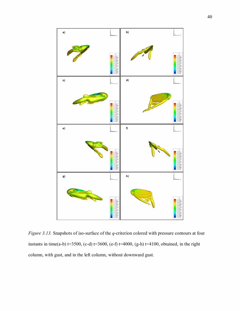
40


instants in time(a-b) t=3500, (c-d) t=3600, (e-f) t=4000, (g-h) t=4100, obtained, in the right

column, with gust, and in the left column, without downward gust.

41

Another conclusion that can be drawn from these gust simulations is that the thrust coefficient

returns to its baseline profile after one flapping cycle once the wind gust is removed. It gives an

indication that if an insect or MAV does encounter a strong downward gust whose velocity is

greater than half of its maximum wing-tip speed, it can effectively recover its baseline hover

dynamics after the wind gust fluctuations have ceased. These results demonstrate the potential of

flapping-wing MAVs to provide a stable flight even in gusty environments.

3.3.3 Side gust. The last cases considered concern the effect of a side gust on the

performance of the same hovering wing considered in the previous two cases. This problem is

particularly interesting, because, to our knowledge, no numerical or experimental results on side

gusts are available in the open literature. In contrast to frontal and downward gusts, which have

the same effect on both wings of an insect or MAV, a side gust generates the different

aerodynamic response of each wing, depending on whether the gust velocity is oriented from the

root of the wing to its tip (referred as RT gust) or the other way around, from tip to root (referred

as TR gust). Both root-to-tip and tip-to-root gusts are considered in the present work. For both

cases, the side gust starts during the 2nd

wing stroke and increases as a sinusoidal pulse, reaching

its maximum value during the 4th

stroke. As in the downward- and frontal-gust cases, the wing

makes 4 full strokes during the wind gust, and the ratio of the gust velocity to the maximum

wing tip velocity is equal to 0.5, which corresponds to the gust amplitude of approximately 3.5

m/s.

First we consider a side gust that is oriented from the wing root to its tip. Time histories

of the flapping wing thrust coefficient computed with and without the presence of the RT gust

are shown in Fig. 3.14. As one can see in the figure, the time-averaged thrust coefficient grows

as the gust velocity increases. The highest peak value of the thrust coefficient occurs near t=4000

42

when the gust velocity reaches its maximum value. Similar to the downward- and frontal-gust

cases, the response time of the flapping wing to the RT gust is shorter than one flapping cycle. It

should also be noted that when the gust is the strongest, the thrust generated by the wing

becomes negative over a small portion of the full stroke. To gain a deeper insight into the flow

physics of the flapping wing in the presence of RT gust, snapshots of an isosurface of the q-

criterion obtained with and without gust are presented in Fig. 3.15. The q-criterion reveals the

vortical flow regions, thus identifying the leading edge, root, and tip vortices. As follows from

Fig. 3.15, the presence of the side wind gust strengthens the leading edge and tip vortices during

both the forward and backward strokes. Another important observation is that the vortex shed

from the wing leading edge in the previous backward or forward stroke is convected towards the

wing by the side gust. These additional vortices influence the flowfield during the next stroke,

thus increasing the amplitude of oscillations of the thrust coefficient.

Figure 3.14. Time histories of the gust velocity and thrust coefficient with and without RT gust.

Time

Thrust

0 2000 4000 6000 8000

0

0.5

1

1.5

2

Root-to-tip gust

No gust

Gust velocity

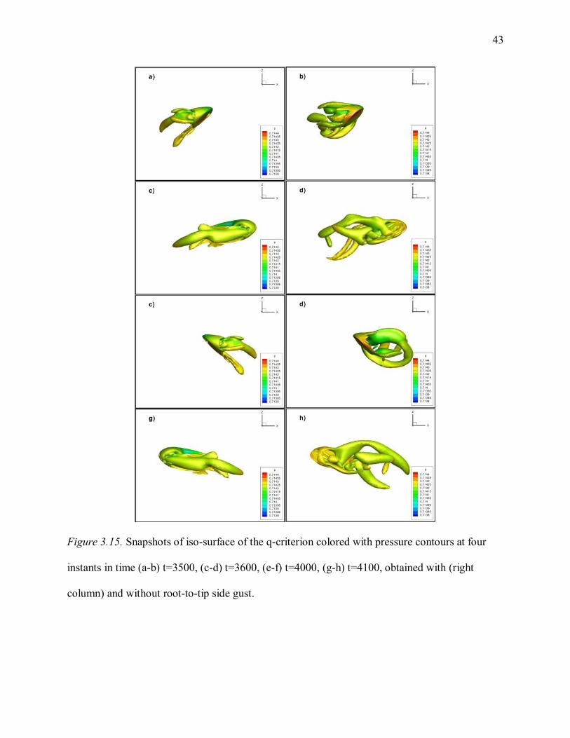
43



column) and without root-to-tip side gust.

44

In contrast to the root-to-tip gust case, there is no significant increase in the amplitude of

the thrust coefficient when the gust velocity is oriented from the wing tip to its root, as evident in

Fig. 3.16. One can observe nonlinearities in the thrust profile in Fig. 3.16, which are not present

in the root-to-tip gust case. Another interesting observation is that there is the phase shift in the

thrust coefficient profile as compared with that in the quiescent flow case, which is caused by the

presence of the side gust.

It should also be noted that the thrust coefficient becomes negative during the stroke

reversals as the wing gust velocity increases. This aerodynamic response of the flapping wing to

the TR side gust can be explained by examining snapshots of an isosurface of the q-criterion,

which are shown in Fig. 3.17. At the end of up- and downward strokes, the wing moves in the

direction that is almost aligned with the gust velocity, so that the relative wing velocity with

respect to the wind gust is significantly lower than that in the quiescent flow. The result is that

the leading edge vortex strength in the presence of the TR gust becomes much lower than its

strength when the side gust is not present, as one can see in Fig. 3.17.

Figure 3.16. Thrust response of the wing in a tip-to-root gust.

Time

Thrust

0 2000 4000 6000 8000-0.2

0

0.2

0.4

0.6

0.8

1

1.2Tip-to-root gust

No gust

Gust velocity

45


instants in time (wing tip-to-root) (a-b) t=3500, (c-d) t=3600, (e-f) t=4000, (g-h) t=4100,

obtained, in the right column, with gust, and in the left column, without side gust.

46

Figure 3.18. Cycle-averaged (over one full stroke) thrust coefficient for the side gust case.

To better understand what effect the RT and TR side gusts have on the flapping wing

performance, we evaluate the cycle-averaged thrust coefficient that is presented in Fig. 3.18. For

the RT case, the cycle–averaged thrust steadily increases over its mean value, thus indicating that

the flapping wing gains thrust under the moderate side wind oriented from the wing root to its

tip. In the presence of the tip-to-root side gust, the cycle-averaged thrust coefficient decreases

reaching its minimum value when the wind velocity is highest. These results indicate that a two-

wing MAV may experience a strong roll rotation in the moderate side gust, because of the

difference in the thrusts generated by each wing, which is caused by the different orientations of

the left and right wings with respect the wind velocity vector.

3.4 Discussion

The performance of a flapping wing under various gust conditions including frontal,

downward, and side gusts has been studied in Chapter 3 by using the 3-D fully unstructured,

unsteady RANS code, FUN3D. As follows from our numerical results, the downward gust

Time


0 2000 4000 6000 80000

0.2

0.4

0.6

0.8

No gust

Root-to-tip gust

Tip-to-root gust

47

drastically reduces the thrust generated by a centimeter-scale flapping wing when the ratio of the

gust velocity to the wing tip velocity is 0.5, thus indicating that small-scale flapping-wing MAVs

may be susceptible to downward gusts. In the case of a frontal gust of the same amplitude used

in the downward case, the peak value of the wing thrust coefficient during the forward (with

respect to the wind direction) stroke exceeds its baseline value by more than a factor of 2.

Though the instantaneous thrust significantly decreases during the backward stroke, the cycle-

averaged thrust coefficient demonstrates an overall increase that is proportional to the wing gust

velocity. These results indicate that flapping-wing MAVs can alleviate frontal gusts whose mean

gust velocity is less than the wing tip velocity. For the side gust case, the thrust generated by a

wing strongly depends on the mutual orientation of the wing and the gust velocity vector. A

significant increase in the time-averaged thrust coefficient is observed in the case when the gust

is oriented from the wing root to its tip. Note, however, that the cycle-averaged thrust coefficient

decreases when the wing experiences the tip-to-root gust of the same amplitude. Though the side

gust has only moderate effect of the wing thrust coefficient, it produces a substantial rolling

moment caused by the difference in the thrusts generated by each wing of an insect or MAV,

thus indicating that the biological or robotic flyer can lose control in the presence of the side

gust. Another interesting observation is that for all types of gusts, the thrust generated by the

flapping wing returns to its baseline profile over just one full stroke once the gust is removed,

thus showing that the flapping wing can effectively recover from wind gust fluctuations.

The numerical results presented above provide a new insight into flapping wing

aerodynamics in the presence of various wind gusts. In contrast to frontal and downward gust

scenarios, the side gust case has not been sufficiently explored in the literature as many studies

only consider two-dimensional airfoils, assuming symmetry over the span of the wing, i.e., two-

48

dimensional gust. Our results shed light on how a bee mitigates and gain control in a side gust

(see Figure 3.19).

Figure 3.19. A bee maneuvering in a side gust.

As one can see in Figure 3.19, three main events occur when a bee experiences a side gust: 1) the

bee noticeably moves in the same direction of the gust, 2) the insect rolls, so that its left wing

goes down, while the right wing goes up, and 3) the bee appears to adjust itself by accomplishing

a maneuver of its entire body to position itself head-on with respect to the wind direction.

The first event can be explained by the drag force of the fluid acting mechanically on the

body of the entire insect. The last two events are of interest for the current discussion.

Interpreting the present results of the single wing in the moderate side gust, we know that there is

the difference in the cycle-averaged thrust generated by each wing, which produces a rolling

moment. This difference in the thrusts generated by the left and right wings rotates the bee in the

counterclockwise direction, as evident in Fig. 3.19. The third event also partially corroborates

our observations for the frontal gust case. Figure 3.19 shows that the bee recovers from the side

gust in an interesting way by positioning itself head-on with respect to the wind gust direction.

This maneuver can be explained by the fact that the cycle-averaged thrust significantly increases

49

in the presence of a frontal gusts. It should be noted that the maneuver performed by the bee is

accomplished using only several strokes of the wings, which also corroborates the recoverability

of the thrust generated by a flapping-wing observed in our wind gust simulations.

50

CHAPTER 4

Adjoint-based Optimization of Flapping–Wing Flows

4.1 Introduction

Insects and small birds represent fully functional examples of efficient small-scale flying

devices. However, mimicking of the wing kinematics and shape of flying animals is far from

being sufficient to design and build effective, highly maneuverable, agile micro air vehicles

(MAVs). Indeed, the current state-of-the-art materials, micro-scale actuators, propulsion systems,

and power sources are different and in most cases less efficient than those found in nature. This

lack in efficiency of currently available MAV components indicates that a different region of the

design space as compared with that of flying insects and animals should be explored to be able to

maximize the performance of flapping-wing microsystems. Therefore, designs inspired by flying

animals can be used only as a preliminary conceptual design that requires further optimization

for constructing efficient and agile flying micro-scale platforms optimized for size, weight,

speed, and maneuverability. This is a very challenging optimization problem that involves

hundreds or even thousands of kinematics and shape design variables and is governed by highly

unsteady vortex-dominated turbulent flows. Therefore, efficient, mathematically rigorous

optimization techniques based on optimal control theory should be used for solving this class of

problems.

In spite of significant progress in modeling and computational fluid dynamics (CFD)

analysis of flapping- and rotary-wing platforms (Platzer & Jones, 2008) (Shyy, et al., 2010)

(Malhan, Lakshminarayan, Baeder, & Chopra, 2011) (Jones & Yamaleev, 2012), questions

related to optimal design of efficient micro air vehicles (MAV) have not yet been properly

addressed especially in three dimensions because of the physics complexity and computational

51

cost involved. Various parametric and sensitivity studies (e.g., see (Platzer & Jones, 2008)) have

revealed that there is an essentially nonlinear relationship between the major wing kinematic

parameters (amplitude, frequency, phase shift angle), shape parameters (wing thickness,

planform, twist, and camber), and global flow parameters (the Reynolds, Strouhal, and Mach

numbers). Conventional parametric studies which estimate the sensitivity to each individual

design variable independently do not take into account this nonlinear relationship between the

main parameters determining the MAV performance. Furthermore, parametric studies are

extremely computationally expensive because of the very large dimensionality of the design

space and therefore impractical for optimization and design of efficient flapping-wing

microsystems.

Several attempts have recently been made to use genetic algorithms based on low-fidelity

models (Hamdaoui, Mouret, Doncieux, & Sagaut, 2008), high-fidelity models (Ito, 2002), and

experimental apparatus (Milano & Gharib, 2005) for optimization of flapping-wing flows. Since

these stochastic optimization techniques require thousands of evaluations of the objective

functional for each design variable, all these approaches have been limited to optimization of 2-

D flows with a very small number (less than 4) of design variables. Gradient-based methods

provide a powerful alternative for optimization of flapping airfoils and wings. Culbreth et al.

(Culbreth, Allaneau, & Jameson, 2011) uses a finite difference method coupled with a 3-D

Navier-Stokes solver to evaluate the sensitivities of a modified propulsive efficiency to 4

spanwise twist design variables. In (Tuncer & Kaya, 2004), a forward mode differentiation

method governed by a 2-D Navier-Stokes solver has been successfully used to maximize thrust

and propulsive efficiency of a pitching and plunging airfoil.

52

Unlike the forward mode differentiation methods which suffer from excessive cost

caused by the need to solve the unsteady Navier-Stokes equations as many times as the number

of design variables, an adjoint method provides the sensitivities at a cost which is comparable to

that of a single flow solution and independent of the number of design variables. Adjoint-based

optimization of flapping wing flows has been very rare and received significantly less attention

(Stanford & Beran, 2011) (Nielsen & Diskin, 2012). In the present work the adjoint based

methodology developed in (Yamaleev, Diskin, & Nielsen, 2008) (Nielsen, Diskin, & Yamaleev,

Discrete Adjoint-Based Design Optimization of Unsteady Turbulent Flows on Dynamic

Unstructured Grids, 2010) is used to optimize the performance of an isolated wing undergoing

insect-based flapping motion. Wing kinematic parameters, such as stroke and pitch angle

amplitudes and frequencies, phase shift angle between pitching and flapping motions as well as

shape parameters (planform, twist, thickness, etc.) are used as design variables. As will be shown

in Section 4.6,4.7, the wing performance significantly increases while all the imposed constraints

are satisfied in the course of optimization, thus indicating that the developed methodology can be

efficiently used for optimization and design of MAV systems.

4.2 Governing Equations and Numerical Method

In contrast to the gust studies for which the flapping-wing flow at very low Mach

numbers is simulated using the low-Mach-number preconditioner, in this chapter, the flow near a

flapping wing is assumed to be incompressible. The main reason for using the different flow

model in our optimization studies is due to the fact the low-Mach-number preconditioner is

available only for use with the flow solver, but its effects have not been accounted for in the

derivation and implementation of the adjoint equations. The artificial compressibility form of the

3-D unsteady Reynolds-Averaged Navier-Stokes (URANS) equations is used for all optimization

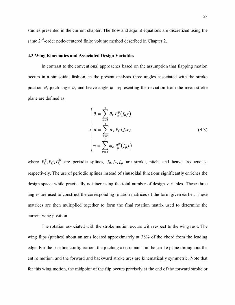
53

studies presented in the current chapter. The flow and adjoint equations are discretized using the

same 2nd

-order node-centered finite volume method described in Chapter 2.

4.3 Wing Kinematics and Associated Design Variables

In contrast to the conventional approaches based on the assumption that flapping motion

occurs in a sinusoidal fashion, in the present analysis three angles associated with the stroke

position , pitch angle , and heave angle representing the deviation from the mean stroke

plane are defined as:

where

are periodic splines, are stroke, pitch, and heave frequencies,

respectively. The use of periodic splines instead of sinusoidal functions significantly enriches the

design space, while practically not increasing the total number of design variables. These three

angles are used to construct the corresponding rotation matrices of the form given earlier. These

matrices are then multiplied together to form the final rotation matrix used to determine the

current wing position.

The rotation associated with the stroke motion occurs with respect to the wing root. The

wing flips (pitches) about an axis located approximately at 38% of the chord from the leading

edge. For the baseline configuration, the pitching axis remains in the stroke plane throughout the

entire motion, and the forward and backward stroke arcs are kinematically symmetric. Note that

for this wing motion, the midpoint of the flip occurs precisely at the end of the forward stroke or

54

the end of the backward stroke. The amplitudes and frequencies in Eq. (4.3) as well as the

coefficients of the periodic splines

are used as design variables and optimized to

maximize the propulsive efficiency of the flapping wing. Along with the lower and upper bounds

for each design variable, the following constraints, which simulate an insect’s wing in hover:

, ,

are imposed on the frequencies for all test cases considered. The above condition provides a

flapping pattern in which the wing deviates in the positive and negative direction from the mean

stroke plane. This wing kinematics is observed in a hovering flight of flying insects.

4.4 Shape Parameterization

A software package called Multidisciplinary Aerodynamic-Structural Shape Optimization

Using Deformation (MASSOUD) developed in (Samareh, 1999) is used to parameterize the

shape of a flapping wing defined by design variables that control planform, twist, thickness,

shear, and camber. MASSOUD provides a very general parameterization of surface grids, which

is critic al for performing user-defined shape optimization. At each design cycle, MASSOUD is

employed to transform the wing surface grid in accordance with new values of the shape design

variables provided by the optimizer. In the current study only planform and twist design

variables are optimized. Though this parameterization also allows for wing thickness, camber,

and shear variations, these design variables are held fixed for all cases considered.

To give the reader a better idea how the planform and twist parameterizations are defined

for the baseline wing geometry, the wing surface mesh at three values of one of the planform and

twist design variables are presented in Figs. 4.1 and 4.2, respectively. Figure 4.1 shows that

changes in the planform design variable significantly increases the wing span and aspect ratio.

55

The variation of the twist design variable within its lower and upper bounds also results in

considerable alterations of the wing shape, as one can see in Fig. 4.2.

Baseline

Medium

Large

Figure 4.1. Wing surface meshes generated by MASSOUD at baseline, medium, and large

values by varying design variable 13 that can control the wing span and aspect ratio.

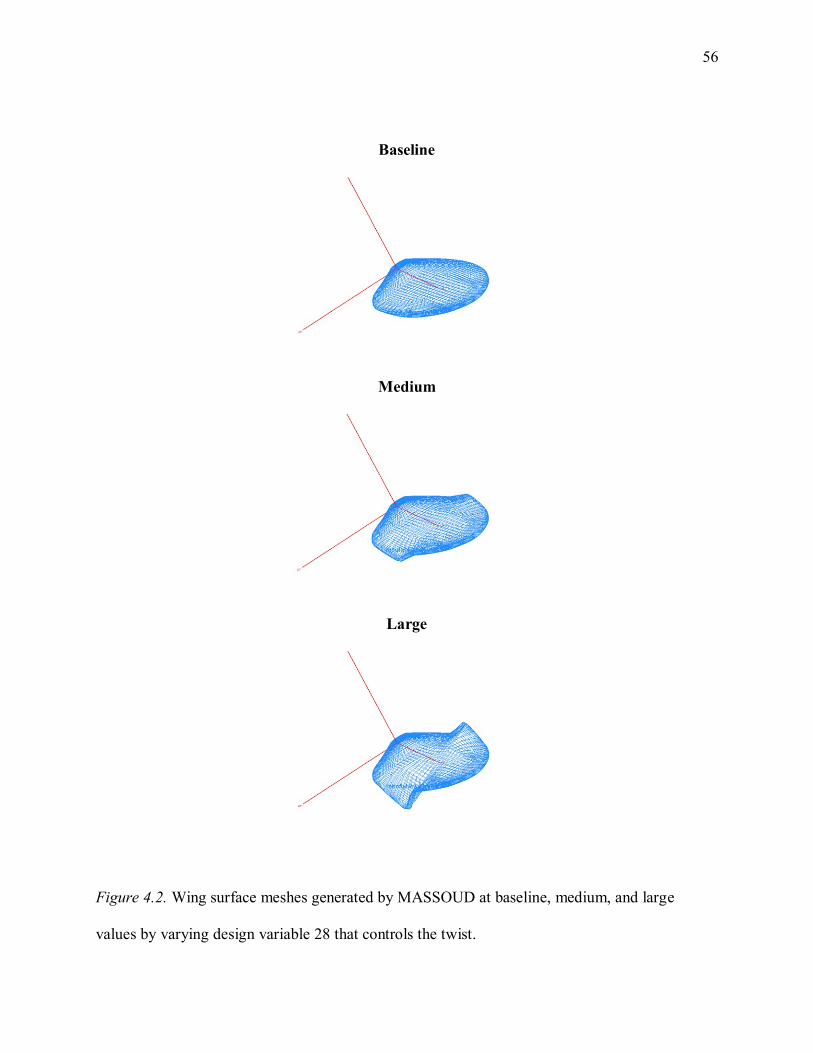
56

Baseline

Medium

Large

Figure 4.2. Wing surface meshes generated by MASSOUD at baseline, medium, and large

values by varying design variable 28 that controls the twist.

57

4.5 Time-Dependent Adjoint-Based Optimization Methodology

Most optimization problems contain the same general factors. These are the state

variables, which are found from the governing equations like the URANS equations; the design

variables that define the design space of the problem; an objective or cost functional; and the

constraints that the state and design variables must simultaneously satisfy.

As has been discussed above, global optimization methods such as stochastic or genetic

algorithms are prohibitively expensive because they require O(104) solves of 3-D URANS

equations, thus making them impractical for solving this large-scale time-dependent optimization

problem. In the present analysis, sensitivity derivatives are computed using the adjoint

formulation implemented in the FUN3D code. A local minimum of the objective functional is

then found by using a gradient method.

To increase the wing performance, an aerodynamic quantity of interest (e.g., thrust, lift,

drag, or their combination) is considered as a functional which is maximized by using optimal

control theory, thus leading to the following discrete PDE-constrained optimization problem:

where D is a vector of the design variables, Qn is a vector of conservative variables,

is a k-th

aerodynamic coefficient such as thrust, lift, drag, or their combination and is its target

value, is a user-defined weighting factor, Nb and Ne are time levels corresponding to a time

58

interval over which the objective functional is minimized, Rn and are the flow and grid

residuals, and is the geometric conservation law term.

The discrete time-dependent optimization problem Eq. (4.4) is solved by the method of

Lagrange multipliers which is used to enforce the flow and grid equations as constraints. The

Lagrangian functional is defined as follows:

where and

are vectors of Lagrange multipliers associated with the flow and grid

equations, respectively, D is a vector of design variables, and for and

Note that terms corresponding to the initial conditions are omitted in Eq. (4.5).

Differentiating the Lagrangian with respect to D, collecting the coefficients of ,

and setting them equal to zero, the following equations for the flow adjoint variables are

derived:

The grid adjoint equations are obtained in a similar way (see (Yamaleev, Diskin, & Nielsen,

2008) for details). The key advantage of the adjoint formulation is that the adjoint equations (4.6)

are independent of the vector D, and should therefore be solved once at each optimization

iteration, regardless of the number of the design variables. Since the first term in Eq. (4.6)

approximates the negative time derivative, the unsteady adjoint equations have to be integrated

backward in time. Therefore, the entire flow solution history should be available during the

59

backward-in-time integration of the flow adjoint equations. In the present approach, the

conservative variables, grid coordinates, and grid velocities are stored to disk at the end of each

time step of the flow solution. During the integration of Eq. (4.6) in reverse time, the stored data

is loaded from disk. With the adjoint variables satisfying the flow and grid adjoint equations, the

gradient of the Lagrangian with respect to D is calculated as follows:

As in Eq. (4.5), terms corresponding to the initial conditions are omitted. A minimum of the

objective functional is found by using a gradient-based optimization package PORT.

Note that the adjoint-based method drastically outperforms other optimization algorithms

in terms of the computational time. Indeed, a gradient method based on the forward mode

differentiation technique requires at least (K+1) solves of the 3-D URANS equations at each

optimization cycle, where K is the number of design variables. For example in our optimization

studies, the CPU time required for solving a flapping-wing optimization problem with 27 design

variables by using the present adjoint-based optimization method on a 8-core workstation is

about 5 days. If this optimization problem is solved on the same workstation by using the

forward mode differentiation method, it would take approximately 4.5 months of CPU time. It

should be emphasized that the CPU time savings would be significantly higher for realistic MAV

configurations parameterized by 1000 or mode design variables.

4.6 Numerical Results

The adjoint-based optimization methodology described above is used to improve the

performance of an isolated flapping wing in hover. The baseline wing resembles a wing profile

of the fruitfly, Drosophila melanogaster, and is based on Dickinson’s et. al. Robofly wing which

60

can be found in (Dickinson & Gotz, 1993). The initial wing geometry has semi-circular leading

and trailing edges, a mean aspect ratio of 2.24, and a thickness-to-chord ratio of 0.04. The

hovering wing is assumed to be operating in quiescent conditions. The baseline Reynolds

number based on the wing maximum tip speed is set equal to 2,000. Our numerical experiments

have shown no appreciable difference between the turbulent and laminar flow solutions and their

adjoints at this relatively small Reynolds number. Therefore, in the present work it is assumed

that the flow is laminar. The baseline kinematic motion consists of two rotations each occurring

at the reduced frequency of 0.236. The first rotation is a stroke motion with amplitude of

600. The second rotation is a pitch motion with amplitude of α 45

0. The stroke and pitch

angles are defined by Eq. (4.3), where the spline coefficients have been selected such that each

rotation very closely approximates a sinusoidal motion. For the baseline configuration, the heave

angle is assumed to be zero over the entire period of flapping motion.

A hexahedral mesh consisting of 251,767 nodes has been used in all numerical

experiments presented in this section. To accurately resolve the boundary layer and vortex

shedding near the wing during the entire flapping motion, the Arbitrary Lagrangian-Eulerian

(ALE) formulation is applied, so that the grid moves rigidly along with the wing. As a result, the

highest grid resolution is achieved in the boundary layer and in the vicinity of the wing during

the entire period of flapping motion, thus significantly reducing the computational cost.

Three optimization cases are considered in the present study. The first case considers

optimization of the wing geometry alone, assuming that the wing kinematics remains fixed and

equal to that of the baseline configuration. The second case optimizes only the wing kinematics,

so that the geometry of the wing does not change in the course of optimization. The third case is

based on the combined optimization of both wing shape and its kinematics. The results obtained

61

for all three cases are compared with each other to evaluate the contribution made by the shape

and kinematic design variables and the nonlinear relationship between these parameters.

A proper choice of the objective functional is critical for not only improving the wing

performance, but also for minimizing the power required for its operation. Note that

maximization of the thrust coefficient alone may also increase the drag, thus indicating that

significantly higher power would be required for operating the optimized flapping wing. To

overcome this problem, the objective functional in Eq. (4.4) for all three cases considered has

been defined as follows:

(4.8)

where and are weight coefficients which are both set to be 5, and C is the coefficient of

force in the x, y, or z directions. Note that the target thrust value is set equal to 10, which is

significantly higher than its baseline value. The last two terms in Eq. (4.8) penalize the objective

functional in such a way that the functional rapidly increases if both Cy and Cz deviate from zero, thus

minimizing the y- and z-components of the aerodynamic force and reducing the power required for the

wing motion in the stroke plane. For all test cases, the wing motion consists of two full strokes.

The time levels Nb and Ne, over which the objective functional given by Eq. (4.4) is minimized,

have been chosen such that they correspond to the second full stroke of the baseline

configuration.

The 3-D discrete primal and adjoint equations are integrated using the BDF2 scheme with

a physical time step corresponding to 150 steps per period of the baseline motion. Forty

subiterations are used at each time step. Each simulation is run for 300 time steps and is

performed on a workstation with the total of 8 processing cores. Approximately 6 gigabytes of

62

disk space are required to store the entire flow solution history. Individual primal and adjoint

solutions require approximately 4 and 3.5 hours of wall-clock time, respectively.

4.7 Shape, Kinematics, and Shape/Kinematics Cases

4.7.1 Shape optimization. The first test case is a design optimization of the baseline

wing undergoing sinusoidal insect-based flapping motion. In the current study, the wing surface

parameterization scheme developed in (Samareh, 1999) is used. This approach uses very general

shape parameterizations of existing surface grids based on a set of design variables such as

planform, twist, thickness, shear, and camber parameters at various locations on the geometry. In

the present work, we use a set of 19 active design variables including 12 variables to control the

wing planform and 7 variables to control the twist. The root section of the wing is held fixed in

all our optimization studies. Upper and lower bounds on each design variable have been chosen

to prevent nonphysical surface shapes. Though this parameterization also allows for wing

thickness, camber, and shear variations, these design variables are held fixed for all cases

considered.

The convergence history of the objective functional given by Eq. (4.8) is shown in Fig.

4.3. The objective functional has been reduced from its initial value of 1282 to a final value of

1147 over 17 design cycles. Note that the major reduction occurs during the first 10 design

cycles after which further improvements are negligible. Closer inspection of the final values of

the design variables reveals moderate changes to all planform parameters and very slight changes

to all twist parameters, thus indicating that the twist has negligible effect on the wing

performance.

63

Figure 4.3 . Convergence history of the objective functional for the first test problem.

The baseline and optimized wing geometries are compared in Fig. 4.4. The optimization

has increased the span of the wing by 40%, while reducing the chord length by nearly 25%.

Another noticeable difference between the planforms of the wing before and after optimization is

a much sharper wing tip of the optimized configuration as compared with that of the baseline

geometry.

Figure 4.4. Planform (left) and cross section of the wing before and after optimization.

Design cycle

Objectivefunctional

0 5 10 15 201240

1250

1260

1270

1280

1290

1300

64

Figure 4.5. Iso-surface of the q-criterion colored with pressure coefficient contours at phase

angles obtained for the baseline (left column) and optimized

wing geometry.

65

The effect of these significant changes in the wing planform on the flowfield can be seen

in Fig. 4.5 that presents snapshots of an iso-surface of the q-criterion obtained for the baseline

and optimal wing geometries at four phase angles during the

second backward stroke. As one can see in Fig. 4.5, the optimized wing geometry significantly

strengthens the leading edge and trailing edge vortices, thus considerably reducing the pressure

in the upper surface of the wing and increasing the thrust. Another interesting observation is that

the leading edge vortex is present along the entire span of the wing, which explains the increase

in the wing span in the course of optimization. As evident in Fig. 4.5, the sharper is the wing tip,

the stronger the vortex it generates over the entire duration of a stroke.

The baseline and optimized thrust profiles are shown in Fig. 4.6(a). The peak value of the

thrust coefficient has been increased by about 100% as compared with its baseline value. Note,

however, that the increase in the propulsive efficiency is significantly less, as one can see

(a) (b)


shape optimization.

Time

Thrust

12 15 18 21 24 27-0.2

0

0.2

0.4

0.6

0.8

1

1.2

1.4

1.6

1.8 Baseline

Optimized

Time

PropulsiveEfficiency

12 15 18 21 24 270

0.2

0.4

0.6

0.8

1Baseline

Optimized

66

in Fig. 4.6(b). In the present study, the propulsive efficiency is evaluated as the thrust-to-drag

ratio. As follows from this comparison, the stroke-averaged propulsive efficiency of the

optimized configuration is about 25% higher than that obtained for the baseline wing geometry.

These results show that optimization of the wing geometry alone provides only minor

improvements in the propulsive efficiency, thus indicating that combined optimization of both

shape and kinematics of the flapping wing is required to significantly increase its performance.

4.7.2 Kinematics optimization. In the second test case, the wing kinematics is optimized

to minimize the same objective functional considered in the previous problem. The stroke, pitch,

and heave angles defining the position of the wing at each moment of time are given by Eq. (5).

Coefficients of the periodic splines in Eq. (4.3), which are associated with the amplitude,

frequency, shape, and symmetry of each angle profile, are used as design variables. Thus, there

are a total of 8 active kinematic design variables for this test case.

(a) (b)


pitch, and heave angles.

67

The convergence history of the objective functional is presented in Fig. 4.7(a). The value

of the objective functional rapidly drops over the first 5 design cycles. The objective functional

reaches its lowest value of 1113 at the 10th design cycle, after which further improvements are

negligible because many of the design variables have reached their bound constraints. The

stroke, pitch, and heave angle profiles before and after the optimization are presented in Fig.

4.7(b). The stroke, pitch, and heave angle amplitudes have been significantly increased during

the optimization, reaching the values of 900, 71

0, and 20

0, respectively. Note that the stroke and

heave angles have reached their upper bound values. The optimizer has also increased the stroke,

pitch and heave frequencies by 13%, so that they attain their upper bound values. The final

values of the other design variables demonstrate moderate changes as compared with their initial

values. One of the key distinctions of the optimal solution from the baseline kinematics is a

significant stroke deviation from the mean stroke plane, which closely resembles a complex

figure-eight stroke path observed in biological flyers. Another important observation that can be

drawn from Fig. 4.7(b) is that both the optimized stroke and pitch angles significantly differ from

their baseline sinusoidal profiles. In contrast to the baseline kinematics, the optimal stroke angle

profile is nearly flat at the stroke ends and significantly steeper in the middle of each stroke,

while the pitch angle demonstrates the opposite behavior. This optimized wing kinematics

obtained using the periodic spline parameterization Eq. (4.3) is different from that observed in

insects and hummingbirds, which is characterized by rapid wing rotation at the end of each

stroke.

68

Figure 4.8. Iso-surface of the q-criterion colored with pressure coefficient contours at phase

angles obtained for the baseline (left column) and optimized

wing kinematics.

69

(a) (b)


optimization.

Snapshots of an iso-surface of the q-criterion colored with pressure coefficient contours

calculated for the baseline and optimized configurations at four phase angles

are shown in Fig. 4.8. As in the previous test case, the leading

and trailing edge vortices generated by the wing with the optimized kinematic parameters are

much stronger than that obtained for the baseline configuration. One of the reasons for

strengthening the leading edge vortex is the increase in the pitch and stroke amplitudes. As one

can see in Fig. 4.8, the 200 deviation from the stroke plane and nearly vertical motion of the wing

at the end of each stroke significantly increase the leading edge vortex strength during the

transition from upward to backward stroke as compared with the baseline configuration. It also

strengthens the wake capture that generates additional aerodynamic forces during stroke

reversals, when the wing rapidly rotates and changes direction.

70

Figure 4.9(a) shows the thrust coefficient obtained using the baseline and optimized wing

kinematics. As follows from this comparison, the peak value of the thrust coefficient over the

second stroke cycle has increased by a factor of 6.5 after the optimization of wing kinematics. In

contrast to the shape optimization, the propulsive efficiency provided by the optimized wing

kinematics is significantly higher than that of the baseline configuration, as evident in Fig.

4.9(b). The peak value of the propulsive efficiency after the optimization has increased by more

than 200% over its baseline value. This drastic improvement in the wing performance is

achieved by using the mathematically rigorous optimization methodology based on the adjoint

formulation. Another important conclusion that can be drawn from this numerical experiment is

that significant increase in the wing propulsive efficiency can be achieved without an appreciable

change in the flapping frequency.

4.7.3 Combined Kinematics and Shape Optimization. The last test case addresses a

very important question on whether even higher performance gains are possible by including

both shape and kinematic design variables into the optimization procedure, thus significantly

expanding the design space that may contain extremum points with higher values of propulsive

efficiency. For this test case, the shape and kinematic design variables are identical to those used

in the previous two cases. Thus, a total number of 27 active variables including 19 shape and 8

kinematic parameters are used for this optimization problem. The same upper and lower bounds

on each design variable have been used to avoid nonphysical wing geometries and kinematics.

Figure 4.10(a) shows a convergence history of the objective functional. Note that the

convergence is slower and less monotonic as compared with the previous two cases. The

optimizer performed 22 flow solutions and 18 adjoint solutions for this test case. The final

stroke, pitch, and heave angle profiles are depicted in Fig. 4.10(b). The optimization has not only

71

(a) (b)


pitch, and heave angles.

increased the magnitude of the peaks of all three angles, but has also altered the frequency such

that it has reached its upper bound. The stroke and pitch angle amplitudes have attained the

values of 900 and 71

0, which are practically identical to those obtained by optimizing the wing

kinematics alone.

Figure 4.11. Planforms (left) and cross sections (right) of the wing before and after combined

optimization of the wing shape and kinematics.

72

Figure 4.12. Iso-surface of the q-criterion at phase angles

obtained for the baseline (left column) and optimized wing kinematics and geometry.

73

(a) (b)


optimization of wing shape and kinematics.

Note, however, that the optimal stroke and pitch angle profiles significantly differ from

those found in the previous case. The wing rotation for the current test case occurs significantly

faster at the end of upstroke and downstroke. Though the optimal solution obtained by the

combined shape-kinematics optimization closely resembles a figure-eight stroke path, the heave

angle amplitude is more than 50% less than its optimal value obtained in the second test case.

The baseline and optimized wing geometries are presented in Fig. 4.11. The span of the wing has

increased by more than 40% after the combined shape-kinematics optimization, which is even

greater than that obtained by optimizing the wing geometry alone. In contrast to the first test

case, the mean chord length, wing tip profile, and twist have not been appreciably changed in the

course of the optimization. Another key distinction between the optimal geometries obtained in

the first and current test cases is that the planform has been rotated such that the axis about which

the wing pitches has been shifted towards the trailing edge and is located approximately at 50%

of the chord. The simultaneous optimization of the wing shape and kinematics results in the

Time

Thrust

12 15 18 21 24 27-1

0

1

2

3

4

5

6

Baseline

Shape

Kinematics

Shape + Kinematics

Time

Propulsiveefficiency

12 15 18 21 24 270

1

2

3

Baseline

Shape

Kinematics

Shape + Kinematics

74

optimal design that is considerably different from that found by optimizing the wing shape and

kinematics independently, thus indicating that there is an essentially nonlinear relationship

between design variables.

Figure 4.12 presents snapshots of an iso-surface of the q-criterion at four phase angles

for the current test case. The combined optimization of the

wing shape and kinematics significantly increases the size and strength of the leading edge and

tip vortices during the entire flapping motion including the rotation stage at the end of each

stroke. The wing-wake interaction is also significantly stronger for the optimized configuration.

The strengthening of the leading edge and tip vortices drastically increase the thrust and

propulsive efficiency generated by the optimized wing as one can see in Figs. 4.13(a) and

4.13(b). As follows from this comparison, the peak values of the thrust coefficient and

propulsive efficiency obtained in the current and previous cases are close to each other and

significantly higher than those provided by the shape optimization alone. Note, however, that in

time-averaged sense, the combined optimization of the wing shape and its kinematics gives the

largest increase in both the wing thrust and propulsive efficiency as one can see in Fig. 14.4. The

optimized stroke-averaged thrust coefficient has been increased by about 70% and 200% over its

value obtained using the individual optimizations of wing kinematics and shape, respectively.

The stroke-averaged propulsive efficiency demonstrates a similar behavior as evident in Fig.

4.14. All these results indicate that the optimization of wing kinematics and its shape should be

performed in a coupled fashion to achieve the maximum improvement in flapping wing

performance.

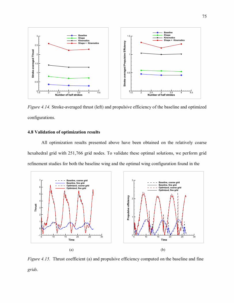
75

Figure 4.14. Stroke-averaged thrust (left) and propulsive efficiency of the baseline and optimized

configurations.

4.8 Validation of optimization results

All optimization results presented above have been obtained on the relatively coarse

hexahedral grid with 251,766 grid nodes. To validate these optimal solutions, we perform grid

refinement studies for both the baseline wing and the optimal wing configuration found in the

(a) (b)

Figure 4.15. Thrust coefficient (a) and propulsive efficiency computed on the baseline and fine

grids.

Number of half strokes

Stroke-averagedThrust

1.5 2 2.5 3 3.5 4 4.50

0.5

1

1.5

2

2.5

3 Baseline

Shape

Kinematics

Shape + Kinematics

Number of half strokes

Stroke-averagedPropulsiveEfficiency

1.5 2 2.5 3 3.5 4 4.50

0.5

1

1.5

Baseline

Shape

Kinematics

Shape + Kinematics

Time

Thrust

5 10 15 20 25 30-1

0

1

2

3

4

5

6

7 Baseline, coarse grid

Baseline, fine grid

Optimized, coarse grid

Optimized, fine grid

Time

Propulsiveefficiency

5 10 15 20 25 300

1

2

3Baseline, coarse grid

Baseline, fine grid

Optimized, coarse grid

Optimized, fine grid

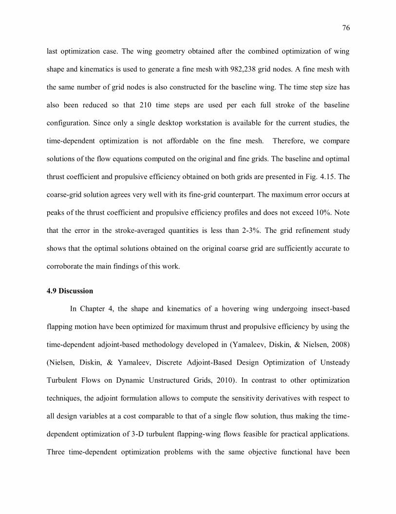
76

last optimization case. The wing geometry obtained after the combined optimization of wing

shape and kinematics is used to generate a fine mesh with 982,238 grid nodes. A fine mesh with

the same number of grid nodes is also constructed for the baseline wing. The time step size has

also been reduced so that 210 time steps are used per each full stroke of the baseline

configuration. Since only a single desktop workstation is available for the current studies, the

time-dependent optimization is not affordable on the fine mesh. Therefore, we compare

solutions of the flow equations computed on the original and fine grids. The baseline and optimal

thrust coefficient and propulsive efficiency obtained on both grids are presented in Fig. 4.15. The

coarse-grid solution agrees very well with its fine-grid counterpart. The maximum error occurs at

peaks of the thrust coefficient and propulsive efficiency profiles and does not exceed 10%. Note

that the error in the stroke-averaged quantities is less than 2-3%. The grid refinement study

shows that the optimal solutions obtained on the original coarse grid are sufficiently accurate to

corroborate the main findings of this work.

4.9 Discussion

In Chapter 4, the shape and kinematics of a hovering wing undergoing insect-based

flapping motion have been optimized for maximum thrust and propulsive efficiency by using the

time-dependent adjoint-based methodology developed in (Yamaleev, Diskin, & Nielsen, 2008)

(Nielsen, Diskin, & Yamaleev, Discrete Adjoint-Based Design Optimization of Unsteady

Turbulent Flows on Dynamic Unstructured Grids, 2010). In contrast to other optimization

techniques, the adjoint formulation allows to compute the sensitivity derivatives with respect to

all design variables at a cost comparable to that of a single flow solution, thus making the time-

dependent optimization of 3-D turbulent flapping-wing flows feasible for practical applications.

Three time-dependent optimization problems with the same objective functional have been

77

considered. The first two cases optimize the wing shape and kinematics which are performed

independently, while the third test case is based on the combined shape-kinematics optimization

of the same baseline flapping wing. The objective functional has been defined such that it

maximizes the wing thrust coefficient and minimizes the drag and consequently the power

required for the wing operation. For the first optimization case, 19 variables including 12

planform and 7 twist parameters are used as design variables. The design variables for the second

problem consists of 8 kinematic parameters including amplitude, frequency, shape, and

parameters determining the symmetry of stroke, pitch and heave angle profiles. The design space

of the third optimization problem consists of both shape and kinematic design variables defined

in the first two cases. For each problem considered, the thrust coefficient has been significantly

improved after the optimization as compared with its baseline value. Note, however, that the

shape optimization alone is not as efficient as the other two optimization strategies. The mean

values of the thrust coefficient obtained by independently optimizing the wing shape and its

kinematics are about 2.1 and 3.9 times higher than the baseline value, respectively. The

simultaneous optimization of the wing shape and kinematics provides even further increase in

the stroke-averaged thrust coefficient which is 70% greater than its maximum value obtained by

the optimization of wing kinematics alone. Similar improvements in the stroke-averaged

propulsive efficiency are observed for all three optimization problems considered. Our numerical

results indicate that there are several factors that play the major role in improving the wing

aerodynamic performance. First of all, the wing span and aspect ratio have been significantly

increased by the shape and shape-kinematics optimization strategies. Note, however, that there

have been no appreciable changes in the wing twist for all cases considered. The second common

trend observed in our numerical experiments is that the stroke, pitch, and heave angle amplitudes

78

have been significantly increased during the optimization. Moreover, the stroke angle amplitude

and all frequencies have reached their upper bound values. The third key distinction of the

optimal solution from the baseline kinematics is that the optimized stroke path closely resembles

a figure-eight shape observed in insects and hummingbirds. Another important conclusion that

can be drawn from our results is that the optimized stroke and pitch angles are characterized by

rapid changes during stroke reversals and significantly different from the corresponding baseline

sinusoidal profiles. All these factors considerably increase the size and strength of the leading

and trailing edge vortices both in the middle of each stroke and during stroke reversals, thus

increasing the pressure difference between windward and leeward sides of the wing. One of the

main conclusions of this work is that the optimal solutions found by optimizing the wing shape

and kinematics independently are quantitatively different from the optimal solution obtained by

solving the optimization problem with the extended design space that includes both the shape

and kinematic design variables. It gives us an indication that there is an essentially nonlinear

relationship between the major kinematic parameters (amplitude, frequency, phase shift angle,

etc.) and shape parameters (wing planform, twist thickness, etc.). These results show that the

time-dependent adjoint-based methodology developed in (Nielsen & Anderson, Aerodynamic

Design Optimization on Unstructured Meshes Using the Navier-Stokes Equations, 1998)

(Yamaleev, Diskin, & Nielsen, 2008) is capable of significantly improving the flapping wing

performance while satisfying the imposed constraints and can be used as a powerful tool for

design and optimization of flapping-wing MAVs.

79

CHAPTER 5

Concluding Remarks and Future Research

5.1 Concluding Remarks

This chapter is set aside to discuss some of the conclusions and outcomes of the research

performed and presented in Chapters 3 and 4. Chapter 3 analyzes the performance of a flapping

wing under various gust conditions including frontal, downward, and side gusts at moderate

wind velocities. Chapter 4 presents novel results on optimization of shape and kinematics of a

flapping wing by using the time-dependent adjoint-based methodology.

5.1.1 Wind gust analysis. The performance of a flapping wing under various gust

conditions including frontal, downward, and side gusts has been studied using the 3-D fully

unstructured URANS code, FUN3D. FUN3D is capable to handle low-speed, low-Reynolds

number flows such as the unsteady turbulent flow near a flapping wing in quiescent air. Very

general grid motions can be defined in FUN3D, which allows us to simulate a gust coming from

any angle with respect to the flapping wing.

The results show that the downward gust drastically reduces the thrust generated by a

centimeter-scale flapping wing when the ratio of the gust velocity to the wing tip velocity is 0.5,

thus indicating that small-scale flapping-wing MAVs may be susceptible to downward gusts. In

the case of a frontal gust of the same amplitude used in the downward case, the peak value of the

wing thrust coefficient during the forward (with respect to the wind direction) stroke exceeds its

baseline value by more than a factor of 2. This increase in thrust is compensated by a similar

reduction during the backward stroke, thus leading to moderate increase in the time-averaged

thrust coefficient. These results indicate that flapping-wing MAVs can alleviate the frontal gust

if the mean gust velocity is less or comparable with the wing tip velocity. A substantial increase

80

in the time-averaged thrust coefficient is observed in the case of the root-to-tip side gust.

However, when the gust is oriented from the wing tip to its root, the cycle-averaged thrust

coefficient decreases in the presence of the side gust. This difference in the aerodynamic

response of the flapping wing generated by the root-to-tip and tip-to-root wind gusts indicate

that, a two-wing MAV may experience a significant rolling moment under side gust conditions.

Another interesting observation is that for all types of gusts, the thrust generated by the flapping

wing returns to its baseline profile over just one full stroke once the gust is removed, thus

showing that the flapping wing can effectively recover from wind gust fluctuations.

5.1.2 Adjoint-based optimization. The shape and kinematics of a hovering wing

undergoing insect-based flapping motion have been optimized for maximum thrust and

propulsive efficiency by using the time-dependent adjoint-based methodology. In contrast to

other optimization techniques, the adjoint formulation allows one to compute the sensitivity

derivatives with respect to all design variables at a cost comparable to that of a single flow

solution, thus making the time-dependent optimization of 3-D turbulent flapping-wing flows

feasible on a single workstation. Three time-dependent optimization problems with the same

objective functional have been considered in the present work. The first two cases optimize the

wing shape and kinematics which are performed independently, while the third case is based on

the combined shape-kinematics optimization of the same baseline flapping wing. The objective

functional has been defined such that it maximizes the wing thrust coefficient and minimizes the

drag and consequently the power required for the wing operation. For the first optimization case,

19 variables including 12 planform and seven twist parameters are used as design variables. The

design variables for the second problem consists of eight kinematic parameters including

amplitude, frequency, shape, and symmetry of stroke, pitch and heave angle profiles.

81

All computations in the optimization study showed significant improvement in thrust and

propulsive efficiency as compared with their baseline values. Interesting to note the nonlinear

relationship between design variables; the kinematic and shape variables considered together

provide much higher increase in the stroke-averaged thrust than that obtained using the

kinematic or shape optimization alone. Though only 27 shape and kinematics design variables

have been used in the present optimization studies, the adjoint-based optimization method can

handle many more design variables and can be used as an efficient tool for design and

optimization of the next generation of flapping-wing MAVs.

5.2 Future Research

Optimization of the performance of a single flapping wing in hover is only the first step

towards building efficient, highly maneuverable MAV systems. The optimal shape and

kinematics of an isolated flapping wing obtained in this dissertation can be used as an initial

guess for optimization of a two-wing-body MAV. In addition to hovering and forward flight

conditions, optimization of a full MAV configuration for maneuverability can also be considered

by using the present adjoint-based methodology. The new adjoint-based optimization capabilities

for overset moving grids available in FUN3D will allow one to maximize the aerodynamic

performance and propulsive efficiency of the entire two-wing-body configuration while

minimizing or constraining the power required for its operation. The developed adjoint-based

technique can be applied not only to determine values of the design variables for optimal MAV

performance, but also to provide the sensitivity derivatives with respect to the kinematic design

variables, which can be used for evaluation of maneuverability and controllability of the

designed MAV. The multi-point optimization procedure can be used for optimal design of

MAVs under various flight conditions. Though the same multi-point strategy can be applied for

82

optimization of wing kinematics, it is expected that for key flight regimes, such as hover,

forward, and maneuvering flights, the multi-point optimization may lead to conflicting

objectives, so that the resulting compromise may hinder the improvement gained. A possible

way to address this problem is to formulate its own wing kinematics optimization problem for

each flight regime (hover, forward, and maneuvering flights). These regimes optimized for

performance can then be incorporated into the MAV flight control system equipped with

appropriate criteria for switching from one regime to another. This approach will maximize the

MAV performance for all important flight regimes. The adjoint-based optimization methodology

can provide not only optimal shape and kinematics of MAV but also the insight into the

mechanisms that control the MAV stability and maneuverability and how the flapping wing

performance is affected by unsteadiness, turbulence, viscosity, and wind gusts during various

flight regimes.

All the results presented in this dissertation have been obtained assuming that the wing is

rigid and the flow is either laminar or fully turbulent. Though these assumptions are sufficient for

conceptual and preliminary design phases of MAVs, a more sophisticated physical model taking

into account aeroelasticity and transition to turbulence effects should be used at the final phase of

the MAV design process. In connection with this, the Computational Structural Dynamics

(CSD) equations and transition models should be coupled with the 3-D URANS equations and

incorporated into the adjoint-based optimization framework. This would require the derivation

and implementation of the adjoint equations for the CSD and transition models. Note, however,

that the computational time and storage cost required for solving this multi-disciplinary

optimization problem may increase significantly. Another very important problem that has not

been properly addressed yet is the incorporation of the adjoint-based gradient methodology into

83

the stochastic optimization framework. It is well known that though the gradient methods are

extremely efficient, they can only provide local extrema of the objective functional. On the other

hand, stochastic optimization algorithms are, in principle, capable of finding global extremum

points, but require thousands of evaluations of the objective functional. One possible direction of

my future research is to combine the best features of both optimization strategies, which will

allow us to find global extrema of the PDE-constrained optimization problem with the

computational cost comparable to that required for gradient-based optimization.

84

References

The Numerical Simulation of Flapping Wings at Low Reynolds Numbers. (2010). AIAA, (pp.

AIAA Paper 2010-724).

Anderson, K. W., & Bonhaus, D. L. (1994). An Implicit Upwind Algorithm for Computing

Turbulent Flows on Unstructured Grids. Computers Fluids, 23(1), 1-21.

Anderson, W. K., & Bonhaus, D. L. (1996). Implicit/Multigrid Algorithms for Incompressible

Turbulent Flows on Unstructured Grids. J. Comput. Physics, 391-408.

Biedron, R. T., & Thomas, J. L. (2009). Recent Enhancements to the FUN3D Flow Solver for

Moving Mesh Applications. AIAA 2009-1360. AIAA.

Biedron, R. T., Vatsa, V. N., & Atkins, H. L. (2005). Simulation of Unsteady Flows Using an

Unstructured Navier-Stokes Solver on Moving and Stationary Grids. 23rd AIAA Applied

Aerodynamics Conference Proceedings. Ontario: AIAA.

Catris, S., & Aupoix, B. (2000). Density Corrections for Turbulence Models. Aerospace Science

and Technology, 1-11.

Culbreth, M., Allaneau, Y., & Jameson, A. (2011). High-Fidelity Optimization of Flapping

Airfoinls and Wings. AIAA, 2011-3521.

Dickinson, M. H., & Gotz, K. G. (1993). Unsteady Aerodynamic Performance of Model Wings

at Low Reynolds Numbers. The Journal of Experimental Biology, 174, 45-64.

Digital Library and Archives. (n.d.). Retrieved March 26, 2013, from etds@vt:

http://scholar.lib.vt.edu/theses/available/etd-110498-110349/

85

Diskin, B., Nishikawa, H., & White, J. A. (2010). Comparison of Node-Centered and Cell-

Centered Unstructured Finite-Volume Discretizations: Viscous Fluxes. AIAA Journal,

48(7).

Dudley, R., & Ellington, C. (1990). Mechanics of Forward Flight in Bumblebees I. Kinematics

and Morphology. Journal of Experimental Biology, 148, 19-52.

Edwards, J. R., & Chandra, S. (1996). Comparison of Eddy Viscosity-Transport Turbulence

Models for Three-Dimensional, Shock-Separated Flowfields. AIAA Journal, 756-763.

Ellington, C. (1999). The Novel Aerodynamics of Insect Flight: Applications to Micro-Air-

Vehicles. The Journal of Experimental Biology, 202, 3439-3448.

Evers, J. H. (2007). Biological Inspiration for Agile Autonomous Air Vehicles. Eglin AFB.

Giles, M. B., & Pierce, N. A. (2000). An Introduction to the Adjoint Approach to Design.

Turbulence and Combustion, 393-415.

Gunzburger, M. D. (2003). Perspectives in Flow Control and Optimization. Philadelphia: SIAM.

Hamdaoui, Mouret, J.-B., Doncieux, S., & Sagaut, P. (2008). Optimization of Kinematics for

Birds and UAVs using Evolutionary Algorithms. Proceedings of the World Academy of

Science, Engineering and Technology, 30.

Ito, K. (2002). Optimization of Flapping Motion. ICAS 2002 Congress.

Jones, M., & Yamaleev, N. (2012). The effect of a gust on the flapping wing performance. AIAA

2012-1080.

Kaufman, L., & Gay, D. (1997). PORT Library: Optimization and Mathematical Programming -

User's Manual. Bell Laboratories.

Kramer, M. (1932). Die Zunahme des Maximalauftriebes von Tragflugeln bei plotzlicher

Anstellwinkelvergrosserung (Boeneffekt). Z. Flugtech. Motorluftschiff, 185-189.

86

Langley Research Center Turbulence Modeling Research. (n.d.). Retrieved March 28, 2013,

from http://turbmodels.larc.nasa.gov

Lian, Y. (2009). Numerical Study of a Flapping Airfoil in Gusty Environments. San Antonio,

Texas, USA: 27th AIAA Applied Aerodynamics Conference.

Liu, H., Ellington, C. P., Kawachi, K., Van den Berg, C., & Willmott, A. P. (1998). A

Computational Fluid Dynamic Study of Hawkmoth Hovering. The Journal of

Experimental Biology, 201, 461-477.

MacCormack, R. W., & Paullay, A. J. (1972). Computational efficiency achieved by time

splitting of finite difference operators. AIAA, (pp. 72-154). San Diego.

Malhan, R., Lakshminarayan, V. K., Baeder, J., & Chopra, I. (2011). CFD investigation of

aerodynamics if rigid flapping wings for MAV applications: Methodology validation.

Pros. of the AHS Specialists Conference. Tempe.

Maxworthy, T. (1979). Experiments on the Weis-Fogh mechanism of lift generation by insects in

hovering flight. Part I. Dynamics of the 'fling'. J. Fluid Mech., 47-63.

McDonald, P. W. (1971). The computation of transonic flow through two-dimensional gas

turbine cascades. ASME.

Milano, M., & Gharib, M. (2005). Uncovering the physics of flapping flat plates with artificial

evolution. J. Fluid Mech., 403-409.

Miller, L. A., & Peskin, C. S. (2005). A Computational Fluid Dynamics of Clap and Fling in the

Smallest Insects. The Journal of Experimental Biology, 195-212.

Monin, A. S., & Yaglom, A. M. (1971). Statistical Fluid Mechanics: Mechanics of Turbulence.

Cambridge: MIT Press.

NASA. (n.d.). Retrieved May 8, 2013, from FUN3D Manual: http://fun3d.larc.nasa.gov/

87

Nielsen, E. J., & Anderson, K. W. (1998). Aerodynamic Design Optimization on Unstructured

Meshes Using the Navier-Stokes Equations. AIAA-98-4809.

Nielsen, E. J., Diskin, B., & Yamaleev, N. K. (2010). Discrete Adjoint-Based Design

Optimization of Unsteady Turbulent Flows on Dynamic Unstructured Grids. AIAA J.,

48(6).

Nielsen, E., & Diskin, B. (2012). Discrete adjoint-based design for unsteady turbulent flows on

dynamic overset unstructured grids. AIAA 2012-0554. AIAA.

Pines, D. J., & Bohorquez, F. (2006, March-April). Challenges Facing Future Micro-Air-Vehicle

Development. Journal of Aircraft, 43(2).

Platzer, M. F., & Jones, K. D. (2008). Flapping-wing Aerodynamics: Progress and Challenges.

AIAA Journal, 46(9), 2136-2149.

Public. (n.d.). Wikipedia. Retrieved April 11, 2013, from Wikipedia: http://www.wikipedia.org

Ramamurti, R., & Sandberg, W. C. (2002). A three-dimensional computational study of the

aerodynamic mechanisms of insect flight. The Journal of Experimental Biology, 205,

1507-1518.

Ramamurti, R., & Sandberg, W. C. (2007). A computational investigation of the three-

dimensional unsteady aerodynamics of Drosophila hovering and maneuvering. The

Journal of Experimental Biology, 210, 881-896.

Ramamurti, R., Sandberg, W. C., & Lohner, R. (2004). The Influence of Fin Rigidity and Gusts

on the Force Production in Fishes and Insects: A Computational Study. Reno, Nevada,

USA: 42nd AIAA Aerospace Sciences Meeting and Exhibit.

Rizzi, A. W., & Inouye, M. (1973). Time split finite volume method for three-dimensional blunt-

body flows. AIAA Journal, 11, 1478-1485.

88

Roe, P. L. (1997). Approximate Riemann Solvers, Parameter Vectors, and Difference Schemes.

Journal of Computational Physics, 250-258.

Rumsey, C. L. (2009). Consistency, Verification, and Validation of Turbulence Models For

Reynolds-Averaged Navier-Stokes Applications. 3rd European Conference fo Aerospace

Sciences.

Rung, T., Bunge, U., Schatz, M., & Thiele, F. (2003). Restatement of the Spalart-Allmaras Eddy-

Viscosity Model in Strain-Adaptive Formulation. AIAA Journal, 1396-1399.

Samareh, J. A. (1999). A Novel Shape Parameterization Approach. NASA.

Sane, S. P. (2003). The aerodynamics of insect flight. The Journal of Experimental Biology, 206,

4191-4208.

Shur, M. L., Strelets, M. K., Travin, A. K., & Spalart, P. R. (2000). Turbulence Modeling in

Rotating and Curved Channels: Assessing the Spalart-Shur Correction. AIAA Journal,

784-792.

Shyy, W., Aono, H., Chimakurthi, K., Trizila, P., Kang, C. K., Cesnik, C., et al. (2010). Recent

progress in flapping wing aerodynamics and aeroelasticity. Progress in Aerospace

Sciences, 46(7), 284-327.

Shyy, W., Lian, Y., Tang, J., Liu, H., Trizila, P., Stanford, B., et al. (2008). Computational

Aerodynamics of Low Reynolds Number Plunging, Pitching and Flexible Wings for

MAV Applicaitons. Reno, Nevada, USA: 46th AIAA Aerospace Sciences Meeting and

Exhibit.

Shyy, W., Lian, Y., Tanga, J., Viieru, D., & Liu, H. (2008). Aerodynamics of Low Reynolds

Number Flyers. New York: Cambridge University Press.

89

Spalart, P. R., & Allmaras, S. R. (1994). A One-Equation Turbulence Model for Aerodynamic

Flows. Recherche Aerospatiale, 5-21.

Stanford, B. K., & Beran, P. S. (2011). Cost reduction techniques for the design of non-linear

flapping wing structures. Int. J. Numer. Meth. Eng., 533-555.

Sun, M., & Tang, J. (2002). Unsteady aerodynamic force generation by a model fruit fly wing in

flapping motion. The Journal of Experimental Biology, 205, 55-70.

Taylor, G. K., Nudds, R. L., & Thomas, A. L. (2003, October 16). Flying and Swimming

Animals Cruise at a Strouhal Number Tuned for High Power Efficiency. Nature, 707-

711.

Thomas, A. L., Taylor, G. K., Srygley, R. B., Nudds, R. L., & Bomphrey, R. J. (2004).

Dragonfly flight: free-flight and tethered flow visualizations reveal a diverse array of

unsteady lift-generating mechanisms, controlled primarily via angle of attack. The

Journal of Experimental Biology, 207, 4299-4323.

Thomas, P. D., & Lombard, C. K. (1978). Geometrical Conservation Law and Its Application.

AIAA J., 1030-1037.

Thompson, M., Watkins, S., White, C., & Holmes, J. (2011, November). Span-wise wind

fluctuations in open terrain as applicable to small flying craft. The Aeronautical Journal,

115(1173), 693-701.

Tuncer, H., & Kaya, M. (2004). Optimization of Flapping Airfoils for Maximum Thrust and

Propulsive Efficiency. Acta Polytechnica, 44(1).

Tuncer, I. H., & Platzer, M. F. (2000, May-June). Computational Study of Flapping Airfoil

Aerodynamics. Journal of Aircraft, 37(3).

90

Turkel, E., & Vatsa, V. N. (2003). Choice of variables and preconditioning for time dependent

problems. AIAA 2003-3692.

Vance, J. T., Faruque, I., & Humbert, J. S. (n.d.). The Effects of Differential Wing Stroke

Amplitude and Stroke Offset on Insect Body Moments During Perturbed Flight

Conditions. Retrieved February 10, 2012, from http://asbweb.org

Viswanath, K., & Tafti, D. K. (2010, September). Effect of Frontal Gusts on Forward Flapping

Flight. AIAA Journal, 48(9).

Wagner, H. (1925). Uber die Entstehung des dynamischen Aufriebes von Tragflugeln. Z. Angew.

Math. Mech., 17-35.

Wan, T., & Huang, C.-k. (2008). Numerical Simulation of Flapping Wing Aerodynamic

Performance Under Gust Wind Conditions. 26th International Congress of the

Aeronautical Sciences.

Watkins, S., Abdulrahim, M., & Shortis, M. (2010). Mitigating the Effects of Atmospheric

Turbulence: Towards More Useful Micro Air Vehicles. Bundoora, Australia.

Watkins, S., Milbank, J., Loxton, B., & Melbourne, W. (2006, November). Atmospheric Winds

and Their Implications for Micro Air Vehicles. AIAA Journal, 44(11), 2591-2600.

Weis-Fogh, T. (1973). Quick estimates of flight fitness in hovering animals, including novel

mechanisms for lift production. J. Exp. Biol., 169-230.

Yamaleev, N., Diskin, B., & Nielsen, E. (2008). Adjoint-based methodology for time-dependent

optimization. AIAA 2008-5857. AIAA.

cfd analysis and design optimization of flapping wing ... · kunigal shivakumar co-advisor sanjiv...

Documents