cfd analysis of sensible thermal energy storage … · gambit® and fluent® as the simulation...

International Journal of Advances in Engineering & Technology, Jan. 2014.

©IJAET ISSN: 22311963

2766 Vol. 6, Issue 6, pp. 2766-2783

CFD ANALYSIS OF SENSIBLE THERMAL ENERGY STORAGE

SYSTEM USING SOLID MEDIUM IN SOLAR THERMAL POWER

PLANT

Meseret Tesfay

Faculty, Department of Mechanical Engineering,

Ethiopian Institute of Technology, [EIT – M], Mekelle University, Ethiopia

ABSTRACT Solar thermal power generation is a modern technology, which has already shown feasible results in the

production of electricity. Thermal energy storage (TES) is an essential feature of solar thermal power plants.

Economic, efficient and reliable thermal energy storage systems are a key need of solar thermal power plants,

in order to smooth out the insolation changes during intermittent cloudy weather condition or during night

period, to allow the operation. To address this goal, based on the parabolic trough power plants, sensible heat

storage system with operation temperature between 3000C – 3900C can be used. The goal of this research is to

design TES which can produce 1MWe. In this work modeling and simulations are performed to analyze two

sensible TES options using Solid medium TES. In this case, different solid sensible thermal energy storage

(STES) systems are investigated and out of all, high-temperature concrete TES and solid NaCl are selected

based on their cost. In addition to this, these two solid medium STESs are simulated using commercial softwares

Gambit® and Fluent® as the simulation tools, in order to optimize the minimum possible size

KEYWORDS: Sensible thermal Energy storage, solar thermal power plant, solid medium, CFD.

I. INTRODUCTION

Solar thermal power generation is a moderately new technology, which has already shown enormous

promise in the production of electricity. Production of electricity from the solar heat energy is by

collecting the direct solar radiation and turning it on solar power technologies to provide medium to

high temperature heat. This heat is then used to operate power cycles, for example through steam

turbines.

However, the electrical output of a solar thermal electric power plant is naturally in a state of change,

due to both predictable and unpredictable time and weather. In either event, the power plant may

require a fully functional storage system to alleviate the changes in solar radiation or to meet demand

peaks. A distinct advantage of solar thermal power plants compared with other renewable energies,

such as photovoltaic (PV) and wind, is the possibility of using relatively cheap storage systems. That

is, reserving the thermal energy itself. Storing electricity is much more expensive [17]. The thermal

energy storage (TES) can store energy in order to shift its delivery time, or to smooth out the plant

output during intermittently cloudy weather conditions. Therefore, thermal storage plays an important

role with the key technologies on economics of energy for the future success of solar thermal

technology.

1.1 Concept of Thermal Energy Storage

Energy storage not only plays an important role in conserving energy but also improves the

performance and reliability of energy systems. In most systems there is an imbalance between the

energy supply and energy demand. The energy storage can even out this mismatch and thereby help in

savings of capital costs [8]. The type and length of mismatch varies from time to time, which



2767 Vol. 6, Issue 6, pp. 2766-2783

influences the type and size of storage. Consider the following cases: Buffer storage: - Sometimes the energy supply from the source may be constant, but there

may be sharp peak load of short duration, as shown in Fig. 1. In this case the amount of

energy to be stored is small. However, the storage has to supply this energy in a very short

time; the rate of energy transfer involved is high. The storage system in such a situation has to

store energy only for short intervals of time and is relatively small in size.

Fig. 1 Constant energy supply at peak load in energy demand [2] Fig. 2 Energy extended over the night

Diurnal storage: - This is required when the load demand is extended typically overnight. As

shown in Fig. 2, in this case solar energy and the load may be constant. Since the energy

supply is zero at night considerable amount of energy must be stored during day time to meet

the demand at night as per the capacity of the storage. The storage must be sufficiently large

to meet the loads in the day time and also to supply energy to the plant for the night.

Seasonal or long term storage: - This storage system is one where solar energy is available

only in summer and the heat load deliver in the winter. As shown in Fig. 3, in this case the

energy collected during an entire season goes to the storage.

Fig. 3 Annual energy storage system

Both buffer and diurnal storages are ‘short term’ storage systems. The design of the storage in this

work will be based on this concept.

1.2 objective

The goal of this research is to design thermal energy storage so that the solar electric generator system

(SEGS) can run for 1hr purely by producing 1MWe in order to extend the working hours of the SEGS

using solar thermal energy. To address this research question, literature survey is done on different

types of TESs. Based on the survey different TES are selected, modeled, designed and simulated using

FLUENT 6.3.26. Finally, optimum dimensions of the TES volume are evaluated.

Notations used:

dc Diameter of the unit model concrete

di Diameter of the hollow on the unit model concrete

G 1x109



2768 Vol. 6, Issue 6, pp. 2766-2783

HTF Heat Transfer Fluid

MWe Mega Watt of electric power

MWt Mega Watt of thermal power

SEGS Solar Electric Generating System

STES Sensible thermal energy storage

TES Thermal energy storage

Eel Electric energy

𝜂el Electrical efficiency

𝜂t Turbine efficiency

Esalt Energy stored on the Solid Salt

Edis Discharged energy

Echar Charged energy

Ec Energy stored on the Concrete

R&D Research and Development

II. MODELLING APPROACH

The Solar Electric Generating System (SEGS) as shown in Fig. 4 is used as the design reference. It

has two parts: the solar cycle and power block cycle. The solar cycle consists of the solar field, which consists of parabolic trough collectors where the

HTF is heated in, the steam generator of the power block, where the oil is to be cooled by evaporating

water in a Rankine cycle, and the thermal storage system now to be designed.

The power block cycle contains the steam generator equipment and the steam turbine that drives the

electric generator, the condenser and the feed pumps. The steam generating system is a set of heat

exchangers which includes a reheater, super-heater, steam generator and pre-heater, and an additional

steam heater, which is used to super-heat during solar energy supply insufficient. The minimum discharge outlet temperature of the TES is dependent on the minimum inlet

temperature of the steam generator. Since the power block will produce only 1MWe, the minimum

inlet temperature to the super-heater is 2500C.

The maximum inlet temperature of the HTF to the TES is depends on the maximum temperature

collected in the field. Since maximum temperature collected in parabolic trough is 3900C – 4000C [3]

in an average daily 7hr insolation as shown in the Fig. 5, the HTF and the storage media are designed

based on this temperature limits.

Fig. 4 model of segs Fig. 5 sharing of energy in the segs

2.1 Physical Storage Model and Theoretical Assumptions

A physical storage model is now presented as shown in Fig. 6. The volume storage system is assumed

to be composed of parallel tubes for the oil passing through it with the storage material around them

which is the solid material concrete. The outer surface of the lane is covered with insulating material.



2769 Vol. 6, Issue 6, pp. 2766-2783

The tube (pipe) wall thickness is not taken into account in the calculation because the thermal

resistance of the pipe is very small when compared to the concrete thickness thermal resistant.

Fig. 6 Physical model

The following assumptions are made for this analysis:

• Thermal losses to the environment are neglected.

• The tubes are parallel and separated by the storage material.

• Each tube is identical.

• The storage unit tube is considered as hollow tube (no steel pipe).

• The tubes are separated from each other at certain pitch.

• The transient temperature distribution is computed for axially symmetry around the tube.

• Temperature effect on the corners of the storage is neglected.

Property of the storage materials are characterized by, the thermal conductivity k, the specific heat

capacity Cp, and the density ρ.

2.2 Governing Equations

There are two phenomena inside this storage:

• Heat transmission from HTF to the concrete

• Heat conduction inside the storage material

Energy balance in a small control volume as shown is Fig. 7.

Fig. 7 Storage physical model

𝐸𝑖𝑛 + 𝐸𝑔𝑒𝑛 − 𝐸𝑜𝑢𝑡 = 𝐸𝑠𝑡𝑜𝑟𝑎𝑔𝑒 (1)

1. Heat transmission from the HTF to the concrete:

−𝑘𝑐∇2𝑇 = ℎ𝑓(𝑇𝑓 − 𝑇𝑤) Between the fluid and concrete (2)

3D transient energy equation and boundary equation governing the heat transfer through the

concrete is:

𝑘𝑐∇2𝑇 + 𝑞′′′ =𝜕

𝜕𝑡𝜌𝐶𝑝𝑇

Oil flow

Inlet

Tw (x, r, ∅)

XL

Out let



2770 Vol. 6, Issue 6, pp. 2766-2783

By neglecting the energy generation, the energy transferred from fluid to the storage is:

𝜕𝑇

𝜕𝑡=

ℎ𝑓

𝜌𝐶𝑝(𝑇𝑓 − 𝑇𝑤) (3)

This equation gives the temperature change of an oil particle that in the case of charging or

discharging of the storage system moves with the velocity 𝑣0 in forward and back ward direction.

2. Heat conduction in the inside the concrete:

The heat conduction inside the concrete is governed by the 3D transient energy equation above,

𝑘𝑐∇2𝑇 =𝜕

𝜕𝑡𝜌𝐶𝑝𝑇. (4)

For axisymmetric situation, Equation 3.7 reduced to:

1

𝑟

𝜕

𝜕𝑟(𝑘𝑟

𝜕𝑇

𝜕𝑟) +

𝜕

𝜕𝑥(𝑘

𝜕𝑇

𝜕𝑥) = 𝜌𝐶𝑝

𝜕𝑇

𝜕𝑡 (5)

This equation gives the amount of energy stored in the volume storage by conduction.

2.3 Storage Efficiency and Utilization Factor

Some estimate values are introduced in order to give objective technical assessment of different

storage system configurations under different design parameters. The storage utilization factor is one

of them, which relates the real energy output on discharge to its theoretically maximum value [4].

𝑈 =𝐸𝑑𝑖𝑠

𝐸𝑚𝑎𝑥 (6)

Storage efficiency is the ratio of energy output to energy input. It represents the heat losses to the

surroundings.

𝜂 =𝐸𝑑𝑖𝑠

𝐸𝑐ℎ𝑎 (7)

2.4 Use of Fluent and Gambit

The storage model, described previously, is simulated using commercial CFD package FLUENT® [6

& 7]. Fluent consists of two separate programs – Gambit and Fluent. Gambit is the pre-processor used

to construct the flow geometry, along with the mesh generation for solving the equations of motion

and continuity. Fluent 6.3.26 is the program which actually solves the equations for the geometries

constructed using Gambit.

2.4.1 Boundary conditions

2.4.1.1 boundary-layer

Boundary layers define the spacing of mesh node rows in regions immediately adjacent to edges

and/or faces as shown in Fig. 8. A good resolution of boundary layers on solid-fluid interface correctly

determines the heat transfer from the fluid to the solid. Based on this, the region close to the wall

between the HTF and storage is handled by taking into consideration this type of meshing.

Fig. 8 Graphical display of boundary layer Grid

2.4.1.2 Wall-Boundary:

The walls are specified with the no-slip boundary condition. In addition to this, thermal boundary

conditions (for heat transfer calculations) and wall roughness (for turbulent flows) are considered.



2771 Vol. 6, Issue 6, pp. 2766-2783

2.4.1.3 Thermal-Boundary

When the energy equation solved on the wall boundary, there are five types of thermal boundary

conditions to be considered.

• Fixed heat flux.

• Fixed temperature.

• Convective heat transfer.

• External radiation heat transfer.

• Combined external radiation and convection heat transfer.

2.4.1.4 Conjugated Heat Transfer Wall Boundary

In view of the fact that the wall boundaries have to assist for energy storage in the volume, a special

wall boundary consideration is required. This ensures simultaneous simulation of convection heat

transfer from the fluid and conduction heat transfer on the solid. This two heat transfer mechanisms

create a coupled effect, and this is done by using conjugated heat transfer on the wall boundary.

𝜕

𝜕𝑡(𝜌ℎ) + ∇. (𝑣𝜌ℎ) = ∇. (𝑘∇𝑇) (8)

The energy flux time scales are different for solid and fluid regions. So, both must be discretized with

appropriate grid size. By creating conjugated wall heat transfer, we compute conduction of heat

through solids, coupled with convective heat transfer in fluid. The coupled boundary condition is

available to any wall zone which separates two cell zones. The meshed wall energy equation is solved

in a solid zone representing the wall. Wall thickness must be meshed. This is the most accurate

approach but requires more meshing effort. And always uses the coupled thermal boundary condition

since there are cells on both sides of the wall.

If the wall thermal resistance calculated without creating coupled thermal condition, the HTF

flows without transferring heat to the storage as shown in the Fig. 9 below, and the storage

volume remains at the ambient temperature.

Fig. 9 Wall only convection heat transfer

However, if the wall thermal resistance is directly accounted for in the energy equation through wall

thickness, the solid temperature is calculated and also the bidirectional heat conduction is calculated

[1]. This is shown in the Fig. 10.

2.4.1.5 Post-Processing

At the end of each solver iteration, the residual sum for each of the conserved variables is computed

and stored, thus recording the convergence history as shown in the Fig. 11.

Solid

((Storage)

HTF



2772 Vol. 6, Issue 6, pp. 2766-2783

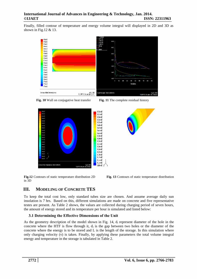
Finally, filled contour of temperature and energy volume integral will displayed in 2D and 3D as

shown in Fig.12 & 13.

Fig. 10 Wall on conjugative heat transfer Fig. 11 The complete residual history

Fig.12 Contours of static temperature distribution 2D Fig. 13 Contours of static temperature distribution

in 3D

III. MODELING OF CONCRETE TES

To keep the total cost low, only standard tubes size are chosen. And assume average daily sun

insolation is 7 hrs. Based on this, different simulations are made on concrete and five representative

testes are present. As Table 2 shows, the values are collected during charging period of seven hours,

the amount of energy stored and its temperature per hour is simulated and listed below:

3.1 Determining the Effective Dimensions of the Unit

As the geometry description of the model shown in Fig. 14, di represent diameter of the hole in the

concrete where the HTF is flow through it, dc is the gap between two holes or the diameter of the

concrete where the energy is to be stored and L is the length of the storage. In this simulation where

only charging velocity (v) is taken. Finally, by applying these parameters the total volume integral

energy and temperature in the storage is tabulated in Table 2.



2773 Vol. 6, Issue 6, pp. 2766-2783

Table 1 Material property

Name Concrete Oil VP-1

Material type Solid [email protected]

Property and Value

Density 2200 kg/m3 755 kg/m3

Cp 850 @ 3500C [J/kg k] 2468 J/kg k

K 1.5@ 3500C [W/m2k] 0.086 w/m k

Viscosity 0.93*10-5 pa s 0.180 * 10-3 pa s

Fig. 14 Geometrical description of the model

Table 2 VALUES with different parameters of concrete to find the effective dimensions

Time

(hr)

Test A Test B Test C Test D Test E

di (cm) 6 8 8 2 2

dc (cm) 15 15 20 8 8

V (m/s) 2.5 2.5 2.5 2.5 1

L (m) 10 10 10 10 20

Energy

(𝐽

𝑘𝑔)(m3)

Storage

Temp.0C

Energy

(𝐽

𝑘𝑔)(m3)

Storage

Temp.0C

Energy

(𝐽

𝑘𝑔)(m3)

Storage

Temp.0C

Energy

(𝐽

𝑘𝑔)(m3)

Storage

Temp.0C

Energy

(𝐽

𝑘𝑔)(m3)

Storage

Temp.0C

1 16640.4 205.35 24111.09 280.17 15314.6 148.4 8254.09 258.6 15905.9 269.09

2 29098.5 284.7 32188.07 353.1 32131.0 215.2 12041.74 337.8 22031.1 339.45

3 36254.5 329.79 37875.41 377.53 45219.7 268.1 12641.7 347.8 26654.9 369.39

4 37699.2 360.32 38499.89 385.79 54892.9 297.6 13277.74 361.8 27578.5 381.01

5 38484.1 371.21 38884.09 388.57 61958.4 322.8 13607.41 375.4 27689.1 384.2

6 38814.2 382.13 39014.27 389.11 65111.2 339.1 13835.87 388.2 28232.1 387.1

7 38958.4 387.11 39058.35 389.1 70872.6 354.4 14540.57 389.1 28866.9 389.46

In this simulation concrete as TES, Therminol VP-1 as HTF and their property as have shown in the

above Table 1are taken. In this Table 2 the values are given per unit hours, that is total volume

integral energy and maximum temperature in the storage. Therefore, comparison is done directly by

analyzing the total volume integral energy stored or by multiplying density of the material with the

total volume integral energy stored in order to get the energy storage in Joules per hour.



2774 Vol. 6, Issue 6, pp. 2766-2783

Fig. 15 Energy distribution Fig. 16 Temperature distribution

The results are compiled in plots as shown in Fig. 15 and Fig. 16. In Tests A, B and C show that

though they have the capacity to store more energy it will be shown later that, during discharging they

drop all this energy in a short period of time 10 to 15 min, and the outlet temperature is low. This is

due to short length and wide diameter of the pipe.

In contrast to the above tests, Test D and E have small diameter. Even though they have less capacity

of storing energy, they stay for long time during discharging. However, Test E is better than Test D,

due to length the longer as, it can store almost double. As a result, it will have long discharging time.

Based on these results, the configuration selected for Test E is further analyzed and it will represent

the entire storage model.

3.2 Refinement on the Concrete TES Size Based on Test E (DI = 0.02M DC=0.08M)

After the standard size of the tube were choosen as tube diameter of 20 mm and concrete diameter of

80 mm, further simulations are done to maximize the energy storage. The results of these simulations

are shown in Table 3.The simulation and modelling was performed for four different lengths of TESs,

and by changing different charging and discharging velocities.

The comparison is done by taking a difference between the energy stored at the end of the 7th hr of

charging and the energy left in the storage after discharging for 1hr till the outlet temperature of the

HTF from the storage is equal to the minimum requirement which is 2750C. And, the more discharged

energy the best in energy storing capacity.

For the shortest tube length of 14 m within the range of charging and discharging the energy stored is

very low. As the length of the tube increases energy storage in the tube also increases. Also, for the

same lenth of the tube by changing the mass flow rate it is possible to optimize the enegy storage

inside the tube.

Based on the simulation summarized in Table 3, a tube length of 20 m is selected with charging

velocity of 0.8 m/s and discharging velocity of 0.4 m/s.

Table 3 Different lengths of TESs

Length

(m)

Charging velocity

(m/s)

Discharging

vel. (m/s)

Time (min) taken for discharging the

stored energy

Discharged

energy (MJ)

14

1

1 20 5.70

0.2 1:05 10.67

15

0.8

0.5 30 7.79

0.8 10 4.40

1 0.2 1:10 11.83

18

0.8

0.3 1:00 13.43

0.5 45 11.88

0.8 15 6.34



2775 Vol. 6, Issue 6, pp. 2766-2783

1 0.2 1:45

20

0.6

0.2 1:10 14.72

0.6 30 5.23

0.8

0.4 1:05 15.93

0.5 50 13.97

0.8 25 9.42

1 0.2 > 1:50

3.3 Charging

To deliver steam at a temperature of 2500C, considering 10% loss in heat exchangers, the oil

temperature is discharged from the storage is at 2750C. Then, this minimum required temperature is

attained at the end of 1hour and 03 minutes of charging time. The energy stored starting from this

time till 7th hr is the useful energy as illustrated in Fig. 17. During the charging temperature and

energy distribution on the concrete are tabulated in Table 4. And the histories of energy storage and

residuals are presented in Fig. 18 and Fig. 19.

Fig. 17 History of temperature on the Concrete

TABLE 4 Charging

Time

(hr)

Max. Static

Temp.(0C)

Min. Static

Temp.(0C)

Total Vol. Integral

Energy(J

Kg) (m3)

Oil Concrete Oil Concrete Oil Concrete

1 389.9 262.06 374.01 199.83 5480.26 15716.701

2 389.9 338.7 383.72 269.15 5562.37 23429.58

3 389.9 369.39 387.31 338.21 5596.38 26688.10

4 389.9 381.73 388.83 356.67 5610.36 28060.83

5 389.9 386.01 388.92 364.12 5616.21 28639.06

6 389.9 388.89 389.32 367.10 5618.78 28885.69

7 389.9 389.46 389.86 369.71 5609.18 28989.87

Total energy stored at the end of the 7th hour

Estored = Total Vol. Integral energy of oil and concrete * density of oil and concrete respectively

= [𝜌 ∗ 𝑣𝑜𝑙. 𝐼𝑛𝑡𝑒𝑔𝑟𝑎𝑙 𝑒𝑛𝑒𝑟𝑔𝑦]𝑜𝑖𝑙 + [𝜌 ∗ 𝑣𝑜𝑙. 𝐼𝑛𝑡𝑒𝑔𝑟𝑎𝑙 𝑒𝑛𝑒𝑟𝑔𝑦]𝑐𝑜𝑛𝑐𝑟𝑒𝑡𝑒

= [755 𝑘𝑔/𝑚3 * 5609.18 𝐽 /𝑘𝑔* (𝑚3)] + [2200 𝑘𝑔/𝑚3 * 28989.87 𝐽/𝑘𝑔*(𝑚3)] = 68.01MJ



2776 Vol. 6, Issue 6, pp. 2766-2783

Fig. 18 History of total energy on Concrete Fig. 19 Residual history

3.4 Discharging

During discharging as shown in Fig. 20 and Fig. 21, the flow direction is changed, inlet temperature is

assumed to be 2650C [4] and velocity at 0.4 m/s. the discharging goes on through till the temperature

of the storage reaches 2750C. This is attained at the end of 1 hr and 05 min. The discharging results

are tabulated in Table 5.

Table 5 Discharging

Time

(min)

Max. Static

Temp.(0C)

Min. Static

Temp.(0C)

Total Vol. Integral

Energy (𝐽

𝐾𝑔) (𝑚3)

Oil Concrete Oil Concrete Oil Concrete

5 295.66 388.5 265 358.38 3918.75 28641.7

15 285.56 379.83 265 338.09 3838.5 27685.85

30 280.16 361.74 265 319.24 3797.12 26137.452

45 277.17 345.22 265 305.4 3773.95 24814.62

60 277.72 331.3 265 294.6 3756.18 23731.811

65 276.9 330.4 265 287.2 3784.47 23681.17

After discharging for 65 min till it reaches the minimum requirement temperature of 2750C, the

energy remain in the storage is:

E = [𝜌 ∗ 𝑣𝑜𝑙. 𝐼𝑛𝑡𝑒𝑔𝑟𝑎𝑙 𝑒𝑛𝑒𝑟𝑔𝑦]𝑐𝑜𝑛𝑐𝑟𝑒𝑡𝑒

= 2200 (𝑘𝑔

𝑚3) * 23681.17 (𝐽

𝑘𝑔)𝑚3 = 52.09 MJ

Then, the discharged energy is the difference between the total energy stored and the energy left on

the storage after discharging of 65 min. Therefore, Edis is 15.93 MJ



2777 Vol. 6, Issue 6, pp. 2766-2783

Fig. 20 History of discharge energy on Concrete Fig. 21 Temperature of discharging on Concrete

3.5 Determination of Size of the Storage

The size of the storage is mainly dependent on the amount of energy to be stored as required by the

power block to run it for continuous 1hr, in order to produce saturated steam at a temperature of

2500C. The required discharge temperature of 2750C is reached at charging time of 1:03hrs.

Therefore, the discharged is 15.93 MJ.

𝑈𝑡𝑖𝑙𝑧𝑎𝑡𝑖𝑜𝑛 (𝑈) =𝐸𝑑𝑖𝑠

∆𝐸𝑚𝑎𝑥

=15.93𝑀𝐽

68.02 𝑀𝐽

= 23.42 %

The storage efficiency is the ratio of energy discharged to the energy charged ( the energy charged

directly from the HTF and the energy stored on the HTF at the end).


𝐸𝑐ℎ𝑎

=15.93 𝑀𝐽

15.93 𝑀𝐽+2.85 𝑀𝐽

= 84.8%

3.6 Number of Tubes

The total number of tubes is calculated from the ratio of total energy required by power block to

produce 1 MW of electricity to useful energy stored in single tube unit.

𝑁𝑜. 𝑜𝑓 𝑡𝑢𝑏𝑒𝑠 =𝐸𝑛𝑒𝑟𝑔𝑦 𝑟𝑒𝑞𝑢𝑖𝑟𝑒𝑑 𝑏𝑦 𝑡ℎ𝑒 𝑇𝑢𝑟𝑏𝑖𝑛𝑒

𝑈𝑠𝑒𝑓𝑢𝑙 𝑒𝑛𝑒𝑟𝑔𝑦 𝑑𝑖𝑠𝑐ℎ𝑎𝑟𝑔𝑒𝑑

=27750𝑀𝐽

15.93 𝑀𝐽

= 1742 𝑇𝑢𝑏𝑒𝑠

3.7 Volume of the Storage

In a rectangular block form, Height = 3.4m, Width = 3.4m and Length = 20m

That is: V = (3.4 x 3.4 x 20) m3

For ease of manufacturing and maintenance, it is proposed to be divided into eight sub part blocks

which contain 225 (15*15) tubes, and each block dimension (total 58 excess tubes): (1.2x 1.2 x 20) m3

This is one of the eight concrete thermal energy storages as shown in the Fig. 22.



2778 Vol. 6, Issue 6, pp. 2766-2783

Fig. 22 One block of Concrete TES

3.8 Modification Using Heat Exchanger Tube

These simulations reveal that using 1mm thickness of heat exchanger tube, the energy storage is

increased by approximately 2% relative to the hollow concrete structure without heat exchanger pipe.

Furthermore, using 5mm thickness of heat exchanger pipe the energy storage increases by

approximate 17% relative to the storage without heat exchanger tube. However, as the thickness of the

pipe increase while the storage capacity increases, the cost of TES also increases. It is estimated that

more than 50% of the cost can be tubing related [15].

Table 6 Property of the steel heat exchanger tube A179 - A179/A179M-90a@ 332.50C [3]

Density 7800 Kg/m3

Spcific heat capacity 550 J/kg.k

Thermal conductivity 35 w/m2.k

IV. MODELING OF SOLID NACL THERMAL ENERGY STORAGE

Only common salt NaCl is useful as solid salt. Its data are given in Table 7. In order to achive a large

density and a high thermal conductivity, in comparison to concrete, the salt must be poured into forms

to produce the storage elements (plates) in the liquid state or melted inside the forms and solidified

afterwards.

The relatively high melting temperature of above 7000C and the large melting energy mean a great

technical and energy expense. In storage systems using common salt NaCl in the solid state as storage

medium, the thermal conductivity is much higher in comparison to concrete.

In order to compare the energy storage capacity of solid NaCl with concrete some assumptions are

made as shown in Fig. 23:

• Model size of 20 m length.

• Equal mass flow rate.

• Equal inlet velocity.

• Equal inlet HTF temperature of 3900C.

Fig. 23 Model of the solid NaCl



2779 Vol. 6, Issue 6, pp. 2766-2783

Table 7 Property of sodium Chloride NaCl [3]

Heat of melting 520kJ/Kg

Melting temp. 800 – 802 0C

Boiling point 1439 0C

Solidification point 798 – 819 0C

Density 2160 Kg/m3

Specific heat capacity @1000C 850 J/(kg.k)

Thermal conductivity 7.0 w/(m.k)

4.1 Charging

To deliver steam at a temperature of 2500C, the oil temperature is discharged from the storage is at

2750C. Then, this minimum required temperature is attained at the end of 43 minutes of charging

time. The energy stored starting from this time till 7th hr is the useful energy as illustrated in Fig. 24.

During the charging temperature and energy distribution on the concrete are tabulated in Table 8. And

the histories of energy storage and residuals are presented in Fig. 25.

Fig. 24 Static temperature on salt Fig. 25 History of total energy on salt

Total energy stored at the end of the 7th hour

Estored = Total Vol. Integral energy of oil and NaCl * density of oil and NaCl repsectively

= [𝜌 ∗ 𝑣𝑜𝑙. 𝐼𝑛𝑡𝑒𝑔𝑟𝑎𝑙 𝑒𝑛𝑒𝑟𝑔𝑦]𝑜𝑖𝑙 + [𝜌 ∗ 𝑣𝑜𝑙. 𝐼𝑛𝑡𝑒𝑔𝑟𝑎𝑙 𝑒𝑛𝑒𝑟𝑔𝑦]𝑁𝑎𝐶𝑙

= [755 𝑘𝑔

𝑚3 * 5620.52 (𝐽

𝑘𝑔)𝑚3] + [2160

𝑘𝑔

𝑚3 * 29038.39( 𝐽

𝑘𝑔)𝑚3] = 66.966 MJ

Table 8 Charging of sold NaCl thermal energy storage

Time

(hr)

Max. Static Temp.(0C) Total Vol. Integral

Energy(𝐽

𝐾𝑔)(m3)

Oil NaCl Oil NaCl

1 389.9 383.6 5570.58 27563.30

2 389.9 389.8 5618.66 28975.52

3 389.9 389.9 5620.45 29035.88

4 390 390.0 5620.52 29038.23

5 390 390.0 5620.53 29038.39

6 390 390.0 5620.53 29038.92

7 390 390.0 5620.52 29038.399



2780 Vol. 6, Issue 6, pp. 2766-2783

4.2 Discharging

During discharging as shown in Fig. 26 and Fig. 27, the flow direction is changed, inlet temperature is

2650C [4] and velocity at 0.4 m/s. the discharging goes on through till the temperature of the storage

reaches 2750C. This is attained at the end of 1 hr. The discharging results are tabulated in Table 9.

Fig. 26 Discharging temperature history on salt Fig. 27 Discharging energy history on salt

The utilization factor for Solid NaCl storage is:

𝑈𝑡𝑖𝑙𝑧𝑎𝑡𝑖𝑜𝑛 (𝑈) =𝐸𝑑𝑖𝑠

∆𝐸𝑚𝑎𝑥

=66.96−43.41

66.96

= 35.17 %

Efficiency of the storage during charging and discharging,


𝐸𝑐ℎ𝑎

=23.55 𝑀𝐽

23.55𝑀𝐽+2.83 𝑀𝐽

= 89.27%

Table 9 Discharging Data

Time

(min)

Max. Static

Temp.(0C)

Total Vol. Integral

Energy (𝐽

𝐾𝑔) (𝑚3)

Oil NaCl Oil NaCl

5 339.4 384.35 4322.7 27941.89

15 314.5 359.3 4081.58 25206.73

30 293.37 326.29 3896.58 22496.83

45 280.93 302.96 3799.20 20956.87

60 273.7 287.69 3748.35 20098.89

4.3 Number of Tubes

The total number of tubes is calculated from the ratio of total energy required by power block to

produce 1MW of electricity to useful energy stored in single tube unit.

𝑁𝑜. 𝑜𝑓 𝑡𝑢𝑏𝑒𝑠 =𝐸𝑛𝑒𝑟𝑔𝑦 𝑟𝑒𝑞𝑢𝑖𝑟𝑒𝑑 𝑏𝑦 𝑡ℎ𝑒 𝑇𝑢𝑟𝑏𝑖𝑛𝑒

𝑈𝑠𝑒𝑓𝑢𝑙 𝑒𝑛𝑒𝑟𝑔𝑦 𝑑𝑖𝑠𝑐ℎ𝑎𝑟𝑔𝑒𝑑

=27750𝑀𝐽

23.55 𝑀𝐽 = 1178 𝑇𝑢𝑏𝑒𝑠

4.4 Volume of the Storage

In a rectangular block form, Height =3.04 m, Width = 2.48 m and Length = 20m

That is: V = (3.04 x 2.48 x 20) m3

For ease of manufacturing and maintenance, it is proposed to be divided into six sub part blocks

which contain 196 (14*14) tubes and each block dimension: (1.12x 1.12 x 20) m3



2781 Vol. 6, Issue 6, pp. 2766-2783

Fig. 28 One block of solid NaCl TES

4.5 Modification Using Heat Exchangers Tube

Using the same modification employed as in the concrete storage, by inserting 1 mm thickness of tube

the thermal energy storage inside the solid NaCl increase by approximately 3.5 % relative to the

previous simulation on solid NaCl without pipe inside.

Because solid NaCl has high thermal conductivity relative to concrete, it has higher efficiency and it

can be charged with in less than 20 min as shown in the simulation Fig. 26 and Fig. 27. However, the

energy storage capacity compare to concret it is 1.5 % less as shown in the Table 4.4 below.

4.6 Pressure Losses

The pressure loss in the tube system, even though it has no effect on the energy storage, is essential to

determine pumping work required.

The pressure loss has two compenents , the hydraulic tube friction component ΔPtube and the part

ΔPform due to other reasons (tube bends, valves, cros-section changes and so on).

4.7 Pressure drop in the circular pipe

Recommendation point of view, concrete storage is suggested. And the summary of the storages are

given in Table 4.4. Hydraulic tube friction:

ΔPtube = ρ ∗ λ ∗L

di∗

Vi2

2 (9)

The friction coefficient 𝜆 for laminar flows with Reynolds number Re < 2300 is given by 𝜆 =64

𝑅𝑒 .

For turbulent flows the roughness of the the tube must be taken into account. A correlation for 𝜆 in

this case is [4]:

1

√𝜆= −2 ∗ log [

2.51

𝑅𝑒∗√𝜆+

𝑜.269 𝐾

𝑑𝑖] (10)

With wall roughness K. Steel tubes have a value of K 0.1mm after long use [3].

Therefore , after simplification

𝜆 =1

[2∗log(𝑑𝑖

𝐾)+1.14]

2 (11)

Pressure loss due to bends can be calculated using:

Δ𝑃𝑏𝑒𝑛𝑑 = 𝜌 ∗ 𝑛𝑏𝑒𝑛𝑑 ∗𝑉𝑖

2

2 (12)

Inlet and outlet pressure losses can be calculated using:

Δ𝑃𝑖𝑛𝑙𝑒𝑡+𝑜𝑢𝑡𝑙𝑒𝑡 ≅ 𝜌 ∗ 𝑉𝑖2 (13)

Hence, the total pressure loss due to friction is calculated as:

∆𝑃𝑡𝑜𝑡 = ∆𝑃𝑡𝑢𝑏𝑒 + ∆𝑃𝑏𝑒𝑛𝑑 + ∆𝑃𝑖𝑛𝑙𝑒𝑡+𝑜𝑢𝑡𝑙𝑒𝑡 (14)

The pumping power can be calculated as:

𝑃 =�̇�Δ𝑃𝑡𝑜𝑡

𝜌𝜂𝑝 (15)

But in this work the pressure loss due to friction only in the tube inside the storage is calculated. The

pressure losses in the bends are other fittings are not evaluated since those details are unknown.

1.12 m

20 m



2782 Vol. 6, Issue 6, pp. 2766-2783

The Reynolds number for the flow inside the tube is found to be 64946. Therefore, for turbulent fully

developed flow, using Equation 13, the friction coefficient can be found out. Finally the pressure loss

in a single tube is found out to be,

ΔPtube = 17253.42 Pa

TABLE 4.4 Summary table of the Concrete & solid NaCl

TES

Media

Material property Energy storage at

the end of 7th hr.

Discharged

energy in 1hr

No. of

tubes

Volume of

the storage

Media cost

($/kg) [1]

Concrete

𝜌 =2200Kg/m3

Cp=850J/kg.k

k = 1.5 w/m3.k

68.02 MJ

15.93

1742

231.2 m3

0.05

Solid

NaCl

𝜌=2160 Kg/m3

Cp=850J/kg.k

k = 7.0 w/m.k

66.96MJ

23.55

1178

150.7 m3

0.15

V. CONCLUSION

Based on the initial assumptions of an average daily 7 hr solar insolation, 1MWe of electric to be

produced and using trough solar collector, a literature survey was done on different types of TES

media in order to design a TES which can supply a saturated steam at 2500C and 40 bar for continues

1 hr. The implementation of this TES is to offer cost reduction on the produced electricity or fuel

consumption. Based on this sensible concrete and NaCl TES is selected because of its feasibility and

easy applicable. In this work modeling and simulations are performed to analyze two sensible TES

options.

In addition to this, these two solid medium STESs are simulated using commercial software Gambit®

and Fluent® as the simulation tools, in order to optimize the minimum possible size.

Some technical issues that relevant from the point of view may be manufacturing and operations of

concrete TES can be resolved by:

• Avoiding formation of gaps between the heat exchanger tubes and the high temperature

concrete block.

• Maximizing heat capacity of the high temperature concrete storage block.

• Optimizing the heat transfer between the heat exchanger tubes and the high temperature

concrete storage during charging and discharging.

• Minimizing thermal cracking on the concrete storage matrix during the charge and discharge

cycles.

• Insulation of the TES to the ground and to the ambient.

• Minimizing pressure losses to minimize parasitic pumping power.

• Minimizing heat exchanger failure due to corrosion

Solid Nacl (Common salt) storage system has a considerably smaller storage volume of 150.7 m3 than

concrete which is 231.2m3, and high efficiency of charging and discharging. However, with solid

NaCl storage the possible physical and technical difficulties are greater, and the manufacturing costs

are also higher than concrete.

As a future work, investigations have to be done on selection of cheapest HTF because currently cost

of the HTF is expensive. In addition, modeling of the sensible solid media which has longer length

than this is also another option, because as the length of the TES increase the heat transfer rate

between HTF and solid media also increase inside the tube. This shows more energy will be stored.

Optimization of heat transfer between the HTF and concrete/solid NaCl using fins on the pipes or by

adding frame wires on the concrete/solid NaCl to enhance the heat transfer inside the solid media has

to be carryout. Furthermore, it is also necessary to investigate on mixture of solid NaCl and phase

change materials (PCM) to improve its thermal energy storage capacity.



2783 Vol. 6, Issue 6, pp. 2766-2783

ACKNOWLEDGEMENT

I am heart fully thankful to my supervisor, Prof. Dr. Bhalchandra Puranik (IIT Bombay) for his

encouragement and guidance towards the successful completion of this project. I would also like to

thank Dr. Meyyappan Venkatesan, Assistant Professor – Thermal Engineering, Mekelle University,

for his encouragement to publish this research paper. Finally I thank all my friends and colleagues for

their support in publishing this paper

REFERENCES

[1]. ANSYS Heat transfer modelling, www.fluentusers.com 08, 2009

[2]. Antoni, G., et.al, 2010. “State of art on high temperature thermal energy storage for power generation part

1-Concepts, materials and modellization.” Renewable and Sustainable Energy Reviews 14 (2010) 31–55.

[3]. Brakmann, G., Aringhoff, R., 2005, “Concentrated solar thermal power-Now!” (ESTIA).

[4]. Dinter, F., Geyer, M., Tamme, R., 1991, “Thermal Energy storage for commercial applications,” Spinger-

Verlag.

[5]. Dincer,I., Rosen, A.,2001. “Thermal energy storage systems and applications” John Wiley & sons, LTD.

[6]. Fluent 6.2 User’s Guide Fluent Inc. Centerra Resource Park 10 Cavendish Court Lebanon, NH 03766

January 2005.

[7]. Gambit tutorial Guide, Centerra Resource Park 10 Cavendish Court Lebanon, NH 03766 January 2005.

[8]. Garg, H.P., Mullick, S.C., Bhargava, A.K., 1985, “Solar Thermal Energy storage,” D.Reidel publishing

company.

[9]. https://engineering.purdue.edu/CTRC/solar_website/solar.htm 04,2010

[10]. http://www.exxon.com/Usa-English/Lubes/Pds/Pds_Files/nause2indexcaloriaht43.pdf 08/02/2010

[11]. http://www.loikitsdistribution.com/files/syltherm-800-technical-data-sheet.pdf, 09,2009

[12]. http://www.powerfromthesun.net/Chapter11/Chapter11.htm 7/1/2010

[13]. http://www.renewable-energy-info.com/solar/csp-thermal-storage.html 12/3/2010

[14]. Kearney, D., et.al.2003. “Assessment of a Molten Salt Heat Transfer Fluid in a Parabolic Trough Solar

Field” National Renewal Energy Laboratory, 1617 Cole Blvd., Golden, CO 80401.

[15]. Michael, G., 2002, “CONTEST concrete thermal energy storage for parabolic trough plants” Deutsches

Zentrum für Luft- und Raumfahrt Plataforma Solar de Almeria Spain.

[16]. Pacheco, J., Showalter, S. 2002 “Development of a Molten-Salt Thermocline Thermal Storage System for

Parabolic Trough Plants” Sandia National Laboratories,1 Solar Thermal Technology Department, Albuquerque,

NM 87185-0703

[17]. Pilkington Solar International, 2000, “Survey of Thermal Storage for Parabolic Trough Power Plants,”

GmbH Cologne, Germany

[18]. Schumann, T.E.W, “Heat Transfer: A liquid flowing through a porous prism” combustion Utilities

Corporation, Linden, N.J.

[19]. Sukhatem, S.P., Nayak, J.K., 2008. “Solar energy principles of thermal collection and storage” 3rd edition

Tata McGraw-Hill Publishing Company Limited New Delhi.

[20]. Tamme, R., 2006. “Thermal energy storage concrete and phase change materials” Deutsches Zentrum

[21]. Tamme, R., Laing, D., Steinmann, W.D., 2004, “Advanced thermal energy storage technology for

parabolic trough” ASME Journal of Solar Energy Engineering 126, 794–800

[22]. Therminol VP-1 http://www.therminol.com/pages/products/vp-1.asp, 09, 2009.

[23]. Francis Agyenim , Neil Hewitt , Philip Eames , Mervyn Smyth, Renewable 1 and Sustainable Energy

Reviews 14 (2010) 615– 628

[24]. Thermal Analysis of Energy storage system for federal facilities using phase change material: a Review,

IRACST – Engineering Science and Technology: An International Journal (ESTIJ), ISSN: 2250-3498, Vol.2,

No. 5, October 2012, 875 - 880

AUTHORS

Meseret Tesfay has obtained his M.Tech – Thermal and Fluids Engineering from Indian

Institute of Technology – Bombay (2010) and his B.Sc. degree in Mechanical Engineering

from Mekelle University, Ethiopia in 2006. He has 5 + years of Experience in teaching and

research. His areas of interest are Refrigeration and Air conditioning, Energy, Solar

Thermal applications, Fluid mechanics etc. He is currently working as Lecturer in the

department of Mechanical Engineering in Mekelle University, Ethiopia and he also heads

the Thermal chair in the department. He also engages himself in various consultancy

projects on RAC.

http://www.fluentusers.com/

https://engineering.purdue.edu/CTRC/solar_website/solar.htm%2004,2010

http://www.exxon.com/Usa-English/Lubes/Pds/Pds_Files/nause2indexcaloriaht43.pdf

http://www.loikitsdistribution.com/files/syltherm-800-technical-data-sheet.pdf

http://www.powerfromthesun.net/Chapter11/Chapter11.htm%207/1/2010

http://www.renewable-energy-info.com/solar/csp-thermal-storage.html%20%2012/3/2010

http://www.therminol.com/pages/products/vp-1.asp

cfd analysis of sensible thermal energy storage … · gambit® and fluent® as the simulation...

Documents