cfd computations for common research model … · cfd computations for common research model ......
TRANSCRIPT

CFD Computations for Common Research Model Using the Code HiFUN
Govindasamy. T & Balan RProject Associates
N. BalakrishnanAssociate Professor
Computational Aerodynamics Laboratory,Department of Aerospace Engineering,
Indian Institute of Science, Bangalore-560012, India
6th AIAA CFD Drag Prediction Workshop, Washington, D.C. USA,
16-17 June 2016

N. Balakrishnan CAd Lab, IISc 2
Outline
● Introduction
● Typical Grids
● Results
● Conclusions

3
Introduction

N. Balakrishnan CAd Lab, IISc 4
Tools employed
● Grid generator: ICEMCFD and TGRID.
● Solver: HiFUN***
● Post-processing software: ENSIGHT and TECPLOT.
*** www.sandi.co.in

N. Balakrishnan CAd Lab, IISc 5
Features of the code- HiFUN
● Unstructured cell centre finite volume methodology.
● Higher order accuracy: linear reconstruction procedure.
● Flux limiting: Venkatakrishnan Limiter.
● Inviscid flux computation: Roe scheme.
● Convergence acceleration: matrix free symmetric Gauss Seidel relaxation procedure.
● The viscous flux discretization: Green–Gauss theorem based diamond path reconstruction.
● Eddy viscosity computation: Spalart Allmaras TM.
● Parallelization: MPI.

N. Balakrishnan CAd Lab, IISc 6
Parallel performance
Sahasrat (Cray XC40) 33 K Xeon cores @ 1 Petaflop
Reference: Parallel performance of HiFUN Solver on Cray XC40 - CAd TN 2015:03

N. Balakrishnan CAd Lab, IISc 7
Computational details: WB: Medium grid with about 45 million field cells
● Computer platform: Sahasrat-Cray-XC40
● Number of processors: 1024
● Operating system: Linux Cray customized OS x86_64
● Compiler: Cray Fortran compilers
● Run time wall clock: 2 hours
● Memory requirement of HiFUN: 45 Gb

8
Typical Grids

N. Balakrishnan CAd Lab, IISc 9
Grid details
● Grids have been generated according to the gridding guidelines provided by the DPW6 committee.
✔ Total grid size,✔ First spacing,✔ 2 layers of constant spacing in viscous padding,✔ No of elements at the T.E✔ Farfield distance✔ Grid spacing reduction between various mesh levels by 0.87, etc.
● Boundary layer is grown using aspect ratio based algorithm.
● 40 percent of the total volume cells inside the viscous padding.
● Body is discretized with triangles and the fluid domain is discretized with prisms, tets, pyramids and hex elements.

N. Balakrishnan CAd Lab, IISc 10
Surface mesh

N. Balakrishnan CAd Lab, IISc 11
Volume mesh
Medium
Medium
Medium
Medium

N. Balakrishnan CAd Lab, IISc 12
Grid details
Grids Total grid size (as per guidelines)
Total grid size (as generated)
No of elements on the body
Tiny ~20 m (0.6 m) 20,020,431 401,782
Coarse ~30 m ( 2 m) 30,011,540 533,098
Medium ~45 m ( 5 m) 45,361,230 720,650
Fine ~70 m (17 m) 68,041,757 961,489
Extra Fine ~100 m (41 m) 100,955,603 1,261,727
Ultra Fine ~150 m (138 m) 151,0268,68 1,648,811
WB configuration
Grids No of layers in the viscous padding
BL max growth rate (on fuselage)
T 22 1.53
C 25 1.45
M 29 1.36
F 33 1.32
XF 38 1.26
UF 44 1.2
Grids Total grid size (as per guidelines)
Total grid size (as generated)
No of elements on the body
Tiny 20-30 m 26,529,525 476,220
Coarse 40-45 m 40,124,341 603,135
Medium 60-70 m 59,997,874 778,759
Fine 85-100 m 90,186,887 1,027,280
Extra Fine 130-150 m 137,947,275 1,454,909
Ultra Fine 190-225 m 200,051,932 1,816,492
WBNP configuration
Values in brackets areDPW5 grid sizes

13
Results:
Grid convergence study: Case 2A & Case 2B

N. Balakrishnan CAd Lab, IISc 14
Density & nutilda residue convergenceWB WBNP

N. Balakrishnan CAd Lab, IISc 15
CL & CD: Iterative convergence
1 counts 1 counts
2 counts 2 counts
WB WBNP

N. Balakrishnan CAd Lab, IISc 16
Grid convergence study

N. Balakrishnan CAd Lab, IISc 17
Grid convergence study
5 counts
5 counts
5 counts

N. Balakrishnan CAd Lab, IISc 18
Grid convergence study
2 counts

N. Balakrishnan CAd Lab, IISc 19
Sectional lift distribution
WB WBNP

N. Balakrishnan CAd Lab, IISc 20
Sectional Moment distribution
WB WBNP

N. Balakrishnan CAd Lab, IISc 21
Sectional lift & moment distribution

N. Balakrishnan CAd Lab, IISc 22
WB: Sectional Cp

N. Balakrishnan CAd Lab, IISc 23
WBNP: Sectional Cp

N. Balakrishnan CAd Lab, IISc 24
WB & WBNP : Sectional Cp

N. Balakrishnan CAd Lab, IISc 25
Nacelle: Sectional Cp
PS4X PS3X
PS2X
PS1XPS6X
PS5X

N. Balakrishnan CAd Lab, IISc 26
Junction bubble: WB
Tiny Coarse Medium
Ultra FineExtra FineFine

N. Balakrishnan CAd Lab, IISc 27
Junction bubble: WBNP
Tiny Coarse Medium
Ultra FineExtra FineFine

N. Balakrishnan CAd Lab, IISc 28
Variation of bubble parameters with gridWB WBNP

29
Case 3: Aero elastic study

N. Balakrishnan CAd Lab, IISc 30
Aero elastic study
20 counts
40 counts

N. Balakrishnan CAd Lab, IISc 31
Aero elastic study
40 counts

N. Balakrishnan CAd Lab, IISc 32
AE study: Sectional Cp distribution
N. Balakrishnan CAd Lab, IISc 33
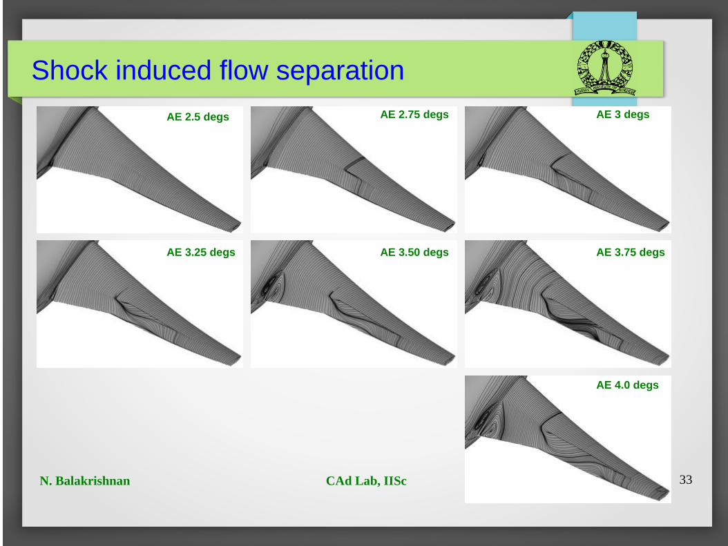
Shock induced flow separation
AE 2.5 degs
AE 3.25 degs AE 3.50 degs AE 3.75 degs
AE 4.0 degs
AE 3 degsAE 2.75 degs

N. Balakrishnan CAd Lab, IISc 34
Junction bubble
AE 2.5 degs
AE 3.25 degs AE 3.50 degs AE 3.75 degs
AE 4.0 degs
AE 3 degsAE 2.75 degs

35
Conclusions

N. Balakrishnan CAd Lab, IISc 36
Concluding remarks
● For the sequence of grids chosen Cp shows less sensitivity.
● Bubble in the Wing-body junction grows with refinement – appears to converge in the last two levels.
● Static Aero-elastic study: lift curve slope change at 3.25 degrees associated with large bubble in the wing-body junction.
Considered Cases: Case 1, Case 2 & Case 3

N. Balakrishnan CAd Lab, IISc 37
Acknowledgments
● Supercomputer Education and Research Centre (SERC), IISc.
● Parthiban Sarath, Ravindra. K, Nikhil Vijay Shende
S&I Engineering Solutions Pvt. Ltd., Bangalore.


39
Case 1
NACA0012: Verification Study

N. Balakrishnan CAd Lab, IISc 40
C-Grid O-Grid
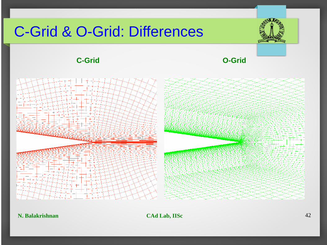
C-Grid & O-Grid: Differences

N. Balakrishnan CAd Lab, IISc 41
C-Grid & O-Grid: Differences
C-Grid O-Grid
N. Balakrishnan CAd Lab, IISc 42
C-Grid & O-Grid: Differences
C-Grid O-Grid

N. Balakrishnan CAd Lab, IISc 43
C-Grid & O-Grid: Differences
Grids Estimated Y plus
First spacing (Mid chord
region)
Growth Rate from
wall
C-Grid Family 2 grid size
O-Grid size
Tiny 2 9.0e-6 m 1.8 3,584 2,296
Coarse 0.82 3.7e-6 m 1.35 14,336 8,942
Medium 0.39 1.7e-6 m 1.16 57,344 35,278
Fine 0.182 8.2e-7 m 1.07 229,376 140,126
Extra-Fine 0.09 4.0e-7 m 1.05 917,504 552,568
Super-Fine 0.045 2.0e-7 m 1.02 3,670,016 2,218,232
Ultra-Fine 0.022 1.0e -7 m 1.0125 14,680,064 8,793,208
Note: In the O grid, the number of points on the body and in radial direction are sameas that in the C-grid.

N. Balakrishnan CAd Lab, IISc 44
Residue convergence

N. Balakrishnan CAd Lab, IISc 45
Iterative convergence
10 counts
10 counts

N. Balakrishnan CAd Lab, IISc 46
Grid convergence study: Forces
5 counts
20 counts

N. Balakrishnan CAd Lab, IISc 47
Grid convergence study: Forces
2 counts
2 counts

N. Balakrishnan CAd Lab, IISc 48
Grid convergence study: Moments
1.2 counts

N. Balakrishnan CAd Lab, IISc 49
Forces & moments comparison
Grids CL CD CDp CDv Cm
3 Codes: FUN3D, CFL3D, TAU
1.0909 - 1.0911 0.01227 - 0.012275 0.00606 - 0.00607 0.006205 - 0.006206 0.00676 - 0.0068
Tiny 1.021969 0.058237 0.053186 0.005050 -0.002947
Coarse 1.074645 0.021022 0.015131 0.005891 0.005683
Medium 1.089100 0.014079 0.007867 0.006212 0.006389
Fine 1.091450 0.012625 0.006319 0.006305 0.006611
Extra-Fine 1.091908 0.012271 0.005932 0.006338 0.006700
Super-Fine 1.092297 0.012217 0.005871 0.006347 0.006632
Ultra-Fine 1.091728 0.012235 0.005868 0.006366 0.006853
