cfd for air induction systems with...
TRANSCRIPT

CFD for air induction systems with OpenFOAMMaster’s thesis in Fluid Mechanics
KLAS FRIDOLIN
Department of Applied MechanicsDivision of Fluid MechanicsCHALMERS UNIVERSITY OF TECHNOLOGYGothenburg, Sweden 2012Master’s thesis 2012:13


MASTER’S THESIS IN FLUID MECHANICS
CFD for air induction systems with OpenFOAM
KLAS FRIDOLIN
Department of Applied Mechanics
Division of Fluid Mechanics
CHALMERS UNIVERSITY OF TECHNOLOGY
Gothenburg, Sweden 2012

CFD for air induction systems with OpenFOAMKLAS FRIDOLIN
c© KLAS FRIDOLIN, 2012
Master’s thesis 2012:13ISSN 1652-8557Department of Applied MechanicsDivision of Fluid MechanicsChalmers University of TechnologySE-412 96 GothenburgSwedenTelephone: +46 (0)31-772 1000
Cover:Air induction system with streamlines coloured by velocity magnitude
Chalmers ReproserviceGothenburg, Sweden 2012
CFD for air induction systems with OpenFOAMMaster’s thesis in Fluid MechanicsKLAS FRIDOLINDepartment of Applied MechanicsDivision of Fluid MechanicsChalmers University of Technology
Abstract
CFD is a very important tool in today’s design of automotive air induction systems. Thesimulations enable the flow in a proposed design to be evaluated without manufacturing thesystem. Most commercial software’s used for this are expensive, and in the ever increasingcompetition lowering costs is a key issue for a carmaker such as Volvo Car Corporation.
This thesis evaluates the use of the open source CFD code OpenFOAM for simulating theflows in air induction systems. Two test cases are used and compared to the commercial codeFluent sold by ANSYS, Inc. The results from both codes are also compared to results fromphysical tests.
Results from the test cases are that although a lot of time has been spent on finding viablenumerical schemes and solver settings, there is still a lot of work to be done before theOpenFOAM simulations show the same numerical stability as the Fluent simulations. Becauseof this and that the same boundary conditions could not be used OF shows results further fromthe experimental results than Fluent. During the project a problem in OpenFOAM concerningoscillating velocities in the interface to porous media was discovered. Put together there is stillwork to be done before OpenFOAM can be used for complete air induction system simulations.
When there is no air filter involved, OpenFOAM is very suitable to use in topology optimi-sation. Since it is command line based it is easy to couple with optimisation software suchas modeFrontier. Also investigated in this thesis is the adjoint solver in OpenFOAM. It is asimple adjoint optimiser but to be truly usable it needs extension. Adjoint optimisation ingeneral is very useful as a guide to designers, but the results are not suitable to use directlysince it doesn’t take variables such as manufacturability into account.
Keywords: CFD, OpenFOAM, Air induction system, porous media, adjoint, topology optimi-sation
i

Sammanfattning
CFD ar idag ett viktigt verktyg vid konstruktion av luftintagssystem till fordon. Simuleringarmojliggor utvardering av konstruktioner utan att tillverka ett fysiskt system. De flesta kom-mersiella programvaror som anvands idag ar dyra, och med den okande konkurrensen inombilindustrin ar laga kostnader mycket viktigt.
Det har arbetet har utvarderat om den oppen kallkods baserade CFD koden OpenFOAM skullekunna anvandas for flodessimuleringar i luftintagssystemen. Tva testsystem har simulerats ochjamforts saval med den kommersiella programvaran Fluent fran ANSYS, Inc. som med fysiskatester.
Resultaten fran testfallen visar att trots att mycket tid lagts pa att fa OpenFOAMsimuleringarnanumeriskt stabila ar de annu inte pa samma niva som simuleringarna dar Fluent har anvants.Detta tillsammans med att samma randvillkor inte kunde anvandas gor att resultaten fran OFligger langre ifran de experimentella matningarna an de som erhallits med Fluent. Ett problemmed OpenFOAM har ocksa upptackts under projektets gang. I gransskiktet till porost media(luftfilter) forekommer icke fysikaliska hastighetsoscillationer. Ovanstaende sammantaget sakravs det fortfarande en del arbete innan OpenFOAM kan anvandas som ersattare till Fluentfor kompletta luftfiltersystemsimuleringar. OpenFOAM ar dock mycket lampligt att anvandavid topologioptimering nar luftfiltret inte behover inkluderas i simuleringen. Eftersom det arkommandoradsbaserat ar det mycket latt att koppla samman med optimeringsprogram sasommodeFrontier. I projektet har ocksa adjointlosaren distribuerad med OpenFOAM undersokts.Det ar en enkel men anvandbar losare men for att vara riktigt anvandbar behover den byggasut. Generellt galler for optimering med adjointmetoden att resultaten ar anvandbara somen guide till konstruktorer men att resultaten inte gar att anvanda rakt av da faktorer somtillverkningsbarhet ej tas i beaktande.
Acknowledgements
First I would like to thank my supervisor Henrik Nyberg at VCC for letting me into the Volvoand open-source CFD worlds. Both very interesting and challenging meaning the learningcurve has been very steep. This makes me thankful for always answering sometimes novicequestions.
Many thanks also goes out to Johan Brunberg and Oscar Bergman, CAE analysts at the airinduction system group for never ending patience when my knowledge hasn’t sufficed. Alsoimportant for the project has been the very helpful nature of Urban Engberg from the VCCCAE support team whom has provided help regarding the computational facilities.
To the rest of the people in the air induction system group, thanks for treating me as one ofyou.
Last but not least, huge thanks to associate professor Hakan Nilsson at Chalmers University ofTechnology for acting as examiner and answering questions.
ii

Nomenclature
Abbreviations
Abbreviation DescriptionAIS Air Induction SystemAMM Air Mass MeterCAD Computer Aided DesignCAE Computer Aided EngineeringCFD Computational Fluid DynamicsMRF Multiple Reference FramesRANS Reynolds Averaged Navier-StokesOpenFOAM Open source Field Operation And ManipulationUI Uniformity IndexURF Under Relaxation FactorVCC Volvo Car Corporation
Roman symbols
Symbol Description Unitscp Specific heat capacity at constant pressure [J/(kgK)]k Turbulent kinetic energy [m2/s2]p Static pressure [Pa]p0 Total pressure [Pa]R Universal gas constant [J/(molK)]T Temperature [K]
Greek symbols
Symbol Description Unitsγ Uniformity index -δij Kronecker delta -η Kolmogorov length scale [m]ε Turbulent energy dissipation rate [m2/s3]µ Dynamic viscosity [Pa s]νη Kolmogorov velocity scale [m/s]τη Kolmogorov time scale [s]Ψ Lagrange multiplier -
iii

iv
Contents
Abstract i
Sammanfattning ii
Acknowledgements ii
Nomenclature iii
Contents v
1 Introduction 11.1 Background . . . . . . . . . . . . . . . . . . . . . . . . . . . . . . . . . . . . . . . 11.2 Objectives . . . . . . . . . . . . . . . . . . . . . . . . . . . . . . . . . . . . . . . . 21.3 Limitations . . . . . . . . . . . . . . . . . . . . . . . . . . . . . . . . . . . . . . . 3
2 Theory 42.1 Fluid mechanics . . . . . . . . . . . . . . . . . . . . . . . . . . . . . . . . . . . . . 42.1.1 Governing equations . . . . . . . . . . . . . . . . . . . . . . . . . . . . . . . . . 42.1.2 Turbulence . . . . . . . . . . . . . . . . . . . . . . . . . . . . . . . . . . . . . . 5
3 Methodology 73.1 Softwares used . . . . . . . . . . . . . . . . . . . . . . . . . . . . . . . . . . . . . 73.1.1 OpenFOAM version 2.1.0 . . . . . . . . . . . . . . . . . . . . . . . . . . . . . . 73.1.2 ANSYS Fluent 14.0 . . . . . . . . . . . . . . . . . . . . . . . . . . . . . . . . . 73.1.3 ANSA version 13.1.5 . . . . . . . . . . . . . . . . . . . . . . . . . . . . . . . . . 73.1.4 ParaView version 3.4.0 . . . . . . . . . . . . . . . . . . . . . . . . . . . . . . . . 73.1.5 CATIA V5 . . . . . . . . . . . . . . . . . . . . . . . . . . . . . . . . . . . . . . 83.1.6 swak4foam version 6.3.7 . . . . . . . . . . . . . . . . . . . . . . . . . . . . . . . 83.2 Air filter system simulations . . . . . . . . . . . . . . . . . . . . . . . . . . . . . . 83.2.1 Simulation setup . . . . . . . . . . . . . . . . . . . . . . . . . . . . . . . . . . . 83.2.2 Comparison with ANSYS Fluent . . . . . . . . . . . . . . . . . . . . . . . . . . 123.2.3 Test case one: I5D P1 . . . . . . . . . . . . . . . . . . . . . . . . . . . . . . . . 133.2.4 Test case two: I5D EuCD . . . . . . . . . . . . . . . . . . . . . . . . . . . . . . 143.2.5 Validation with experiments . . . . . . . . . . . . . . . . . . . . . . . . . . . . . 153.3 Topology optimisation . . . . . . . . . . . . . . . . . . . . . . . . . . . . . . . . . 153.3.1 Adjoint method . . . . . . . . . . . . . . . . . . . . . . . . . . . . . . . . . . . . 163.3.2 Adjoint method and OpenFOAM . . . . . . . . . . . . . . . . . . . . . . . . . . 17
4 Results 194.1 OpenFOAM settings . . . . . . . . . . . . . . . . . . . . . . . . . . . . . . . . . . 194.2 Fluent - OpenFOAM comparison . . . . . . . . . . . . . . . . . . . . . . . . . . . 214.2.1 Case one: I5D P1 . . . . . . . . . . . . . . . . . . . . . . . . . . . . . . . . . . . 214.2.2 Case two: I5D EuCD . . . . . . . . . . . . . . . . . . . . . . . . . . . . . . . . . 244.2.3 Oscillating velocity at porous interface . . . . . . . . . . . . . . . . . . . . . . . 284.3 Validation with experiments . . . . . . . . . . . . . . . . . . . . . . . . . . . . . . 29
v

4.4 Parallel scaling . . . . . . . . . . . . . . . . . . . . . . . . . . . . . . . . . . . . . 294.5 Topology optimisation . . . . . . . . . . . . . . . . . . . . . . . . . . . . . . . . . 30
5 Discussion and conclusions 325.1 System simulations . . . . . . . . . . . . . . . . . . . . . . . . . . . . . . . . . . . 325.2 Topology Optimisation . . . . . . . . . . . . . . . . . . . . . . . . . . . . . . . . . 33
6 Recommendations for further work 35
References 35
A Introduction to OpenFOAM 37A.1 Case setup . . . . . . . . . . . . . . . . . . . . . . . . . . . . . . . . . . . . . . . . 38
B swak4foam script 41
C Python script 43
vi
CHAPTER 1. INTRODUCTION
1 Introduction
1.1 Background
In the beginning of the life of the car, oil was cheap and seemed endless and no one had heardof greenhouse gases or global warming. In recent years though, more and more people havebecome aware of these things and the price of oil has increased a lot during the past decades.This has driven consumers to request more fuel efficient cars and therefore the automotiveindustry puts a great deal of effort into reducing the fuel consumption of their engines. Betterfuel economy brings several advantages with it such as longer range, a lower fuel bill for thevehicle owner and less pollution. But, probably the greatest advantage is that it makes thepetrol/diesel powered car a more sustainable transport solution. One of the many steps inreducing engine fuel consumption is reducing the pressure losses in the air induction system.In the air induction system high airflows have to be reached while keeping the pressure lossesat a minimum. The important functions of the air induction system can be described in thefollowing points:
• Transport the air needed for combustion to the engine within specified leakage limits.
• Reduce noise to levels decided by regulations or VCC.
• Clean the air from dust and dirt.
• Prohibit snow and water intrusion.
• Maintain a favourable profile of the flow with a pressure drop within an acceptable level.
The problem is that the ducting of the air induction system has strict packaging constraintsto fit under the hood of the car together with all the other systems present in a modern car.Figure 1.1.1 shows an example of the complicated topologies required for the air inductionsystem to fit under the hood.
VCC has a group called AIS which is responsible for the air induction system including the airfilter and resonators but not intercoolers in the case of forced induction engines. The groupuses CFD simulations to predict the flow in the ducts and to estimate the pressure loss andvelocity uniformity before the filter (for maximum filter utilisation), before the air mass meterand at the outlet. Of course, the simulations are verified by physical testing in a flow rig beforethey reach production status.
In todays CAE work the limiting factor on the amount of simulations possible are the numberof licenses for the softwares used. As a solution to this problem VCC wants to examine thepossibilities of using the open source software OpenFOAM to carry out some of the CFDsimulations. This would lead to both lower costs for software licenses and better utilisation ofavailable hardware resources. As a first step OpenFOAM would likely be used for optimisationruns where lots of software licences are often required to achieve reasonable lead times.
, Applied mechanics, Master’s Thesis 2012:13 1

1.2. OBJECTIVES CHAPTER 1. INTRODUCTION
Figure 1.1.1: Air induction system for the 5 cylinder diesel engine in the Volvo EuCD platform
1.2 Objectives
The main objective is to assess if OpenFOAM with satisfying results can simulate the flowin air induction systems. The results are to be compared both against existing simulationsusing commercial software (mainly ANSYS Fluent) and against results from experiments. TheOpenFOAM method will involve necessary pre-processing steps, (identification of boundaryconditions, mesh conversion/merging etc.), compressible/incompressible and temperature de-pendant simulations of ducts and filter systems and necessary post-processing steps. Importantdata from post processing include uniformity index and total pressure losses. It is also of greatimportance that the developed method is relatively simple to use as it otherwise will be tootime-consuming to use in day-to-day work.
If OpenFOAM is deemed a feasible software to use for the air induction system simulations,the next step is the investigation of topology optimisation methods using OpenFOAM. Thiswill require a study of optimisation methods to decide which one to use in conjunction withOpenFOAM. The optimisation would focus on finding the optimal design with regard tominimising pressure losses while at the same time achieving high flow uniformity with givenpackaging constraints.
2 , Applied mechanics, Master’s Thesis 2012:13

1.3. LIMITATIONS CHAPTER 1. INTRODUCTION
1.3 Limitations
The evaluation of OpenFOAM as a computational tool is restricted to the air induction systemsonly. The thesis will not try to improve existing calculation methods by, for example, using anew turbulence model, but instead try to replicate them using OpenFOAM.
OpenFOAM is open source and it is therefore possible to make changes to the code and changethe functionality to suit most needs. This is one of the great advantages with OpenFOAM,but outside of the scope of this thesis. Instead the focus will be on evaluating the performanceof existing functionality and as such changes in the code will not be made.
, Applied mechanics, Master’s Thesis 2012:13 3

CHAPTER 2. THEORY
2 Theory
This chapter will present a brief introduction to the theory used in this thesis. Considering thevast size of the field of fluid mechanics, focus will be on aspects relevant for the work carriedout.
2.1 Fluid mechanics
A fluid is a substance that is unable to support shear stresses [1], though in reality they canwithstand some because of viscosity. The study of fluids is called fluid mechanics, and the partof fluid mechanics used here is called fluid dynamics and studies forces in conjunction withfluids.
2.1.1 Governing equations
Fluid flows are well described by the Navier-Stokes equations (eq. 2.1.1), also called themomentum equations since they describe the relation between momentum, pressure and viscousforces in a fluid.
∂
∂t(ρvi) +
∂
∂xj(ρvivj) = − ∂p
∂vi+
∂
∂xj
(µ
(∂vi∂xj
+∂uj∂xi
))+ SM (2.1.1)
The momentum equations (one equation in each coordinate direction) together with thecontinuity equation (eq. 2.1.2), energy equation (eq. 2.1.3) and an equation of state (theperfect gas law has been used in this thesis, eq. 2.1.4)can be seen as the governing equationsof compressible fluid dynamics.
∂
∂t(ρui) +
∂
∂xj= 0 (2.1.2)
∂(ρi)
∂t+
∂
∂xj(ρivj) = −p∂vj
∂xj+
∂
∂xj
(k∂T
∂xi
)+ Φ + Si (2.1.3)
p = ρRT (2.1.4)
If the flow is incompressible and temperature independent only the Navier-Stokes and continuityequation are needed. In this thesis, both incompressible and compressible flows are used, sincethe flow speeds can be higher than Mach 0.3 in thinner sections.
A flow is either laminar or turbulent, with the Reynolds number being the deciding factor.When the Reynolds number of a flow is above a certain critical value the flow becomes turbulent.
4 , Applied mechanics, Master’s Thesis 2012:13

2.1. FLUID MECHANICS CHAPTER 2. THEORY
2.1.2 Turbulence
In laminar flow the adjacent layers slide past each other in an orderly fashion. Turbulent flowon the other hand is random and chaotic in its nature. There are six main characteristics forturbulent flow:
• Irregular
• Diffusive
• Has a relatively high Reynolds number
• Three-dimensional
• Dissipative
• Property of the flow (i.e. not the fluid)
In turbulence unsteady vortices called eddies appear. The largest eddies extract energy fromthe mean flow, called turbulent kinetic energy. This energy is then transferred to smaller andsmaller eddies until it reaches the smallest ones where it is dissipated into heat. This processof energy transfer is called the cascade process. The scale of the smallest eddies are calledthe Kolmogorov scales and where defined in 1941 by A.N. Kolmogorov [2]. There are threeKolmogorov scales: length, velocity and time and they are defined as :
η =
(ε3
ν
) 14
(2.1.5)
τη =( εν
) 12
(2.1.6)
υη = (νε)14 (2.1.7)
In theory one could resolve all of the turbulent scales. The problem with this is that theKolmogorov scales are usually very small which means that this would require a tremendousamount of computing power and memory. Therefore resolving all the turbulent scales is only anoption (with todays computers) for simple problems with low Reynolds numbers. To computemore realistic problems some kind of turbulence modelling has to be used.
Reynolds Averaged Navier-Stokes
The Reynolds averaged Navier-Stokes (RANS) equations are time-averaged versions of theoriginal equations. They are obtained by introducing the Reynolds decomposition of thepressure and velocity and then time-averaging the equations. The Reynolds decompositionconsists of dividing the instantaneous pressure and velocity into one time-averaged and onefluctuating part, i.e.
u = U + u′ (2.1.8)
, Applied mechanics, Master’s Thesis 2012:13 5

2.1. FLUID MECHANICS CHAPTER 2. THEORY
p = P + p′ (2.1.9)
After insertion of the decomposition and time-averaging of the Navier-Stokes equations oneadditional term appears, −ρu′iu′j. This term is called the Reynolds stress tensor and meansadditional unknowns have been introduced. Since the number of equations has not increased,this creates a closure problem. To solve this the Reynolds stress tensor can be modelled usingan eddy viscosity and the velocity gradients. This is called the Boussinesq assumption (Eq.2.1.10) and the basic idea behind it is to model the small-scale eddies with a viscosity term.
−ρu′iu′j = µt
(∂ui∂xj
+∂uj∂xi− 2
3
∂uk∂xk
δij
)− 2
3kδij (2.1.10)
δij is the Kronecker delta and k is the turbulent kinetic energy defined as
k =1
2
(u′2 + v′2 + w′2
)(2.1.11)
There are plenty of models to describe the turbulent quantities including one-equation models,two-equation models and algebraic models.
Realizable k − ε model
To compute the turbulent quantities the realizable k − ε model is normally used at VCC, andas such also in this thesis. The realizable k − ε model is a two-equation model by Jones andLaunder [3] with one equation for k and one for ε. The turbulent dissipation rate ε is a smallscale variable but it is here used as the dissipation rate for large eddies. This is possible becausethe dissipation rate of the small eddies matches the rate at which the large eddies extractenergy from the mean flow through the energy spectrum [4]. The two additional transportequations for k and ε are defined in equation 2.1.12 and 2.1.13 respectively.
∂
∂t(ρk) +
∂
∂xi(ρkui) =
∂
∂xj
[(µ+
µtσk
)∂k
∂xj
]+ P − ρε (2.1.12)
∂
∂t(ρε) +
∂
∂xj(ρεuj) =
∂
∂xj
[(µ+
µtσε
)∂ε
∂xj
]+ ρC1Sε− ρC2
ε2
k +√νε
+ C1εε
k(2.1.13)
where
C1ε = max[0.43, η
η+5
], η = S k
ε, S =
√2SijSij, µt = ρCµ
k2
εand Cµ = 1
A0+As
kU∗
ε
The model constants as specified in OpenFOAM are the following: Cµ = 0.09, A0 = 4, C2 = 1.9,σk = 1 and σε = 1.2. For further details of the realizable k − ε model, please see Jones andLaunder [3].
6 , Applied mechanics, Master’s Thesis 2012:13
CHAPTER 3. METHODOLOGY
3 Methodology
This chapter contains a brief description of the softwares used, a description of how the airfilter system simulations were setup and an introduction of the adjoint method.
3.1 Softwares used
3.1.1 OpenFOAM version 2.1.0
OpenFOAM is in this thesis being evaluated as a CFD solver for air induction systems, butit is more than that. The core of OpenFOAM is a C++ toolbox that enables the creationof customised numerical solvers. The distribution also contains a wide selection of solversdesigned to solve specific problems. For more information on OpenFOAM and how to set up acase, please see appendix A.
3.1.2 ANSYS Fluent 14.0
The currently used CFD software for flow calculations in the air induction system group is thecommercial package Fluent. It contains a variety of physical modelling capabilities to modelmost kinds of flow situations encountered in engineering. Fluent is the software against whichthe OpenFOAM calculations in this thesis have been compared.
3.1.3 ANSA version 13.1.5
ANSA is the pre-processing tool of choice for meshing the air induction systems. Models arecreated in the CAD system CATIA V5 and imported into ANSA for meshing. One of thegreat advantages of ANSA for this thesis project is that it can export meshes directly intoOpenFOAM format. This means that it generates the file structure of an OpenFOAM casedirectly. It is also possible to set some solver settings in ANSA, although the selection ofsolvers isn’t complete.
3.1.4 ParaView version 3.4.0
This is the main post-processing software distributed with OpenFOAM. It is an open-sourcedata analysis and visualisation tool and it can either be invoked by using paraFoam wrapperscript or by converting the data to VTK format and open with ParaView. Data processingcan be done either interactively in a 3D environment or using command line batch processing.
, Applied mechanics, Master’s Thesis 2012:13 7

3.2. AIR FILTER SYSTEM SIMULATIONS CHAPTER 3. METHODOLOGY
3.1.5 CATIA V5
CATIA is a CAD/CAE/CAM system developed by Dassault Systemes. It is widely used inthe automotive and aerospace industries and is also the primary CAD system used at VCC. Inthis thesis it has been used to create the models of the air induction systems simulated.
3.1.6 swak4foam version 6.3.7
Swak4foam stands for ”Swiss Army Knife for Foam” and is a set of libraries and utilities toperform various kinds of data manipulation and representation. It can be used to set complicatedboundary conditions depending on expressions. In this thesis the part of swak4foam thatcontains extended functionObjects (used to perform calculations after each iteration) has beenused to compute total pressure and uniformity index at internal sections.
3.2 Air filter system simulations
The currently performed air filter simulations are run as steady state simulations in severalstages. This is because it can be difficult to reach convergence if all of the options such assecond order accurate numerical schemes were to be used from the start of the simulation. Asstated in section 1.3 this thesis is not about improving existing simulation methods, but theywill be used as a starting point when setting up the OpenFOAM simulations. Fluent has beenused for a relatively long time at the department and boundary conditions etc. are tweakedto suit this software package, which is why all options can not be directly used with anothersoftware package.
3.2.1 Simulation setup
Geometry and mesh generation
The models used are created in the CAD system CATIA V5 and the computational mesh iscreated in ANSA. The geometry is split up into separate volumes with interior surfaces inbetween. This is to simplify volume meshing and also to get interior surfaces which can beused for evaluation. Also, the air filter itself must be a separate cellZone for the solver to knowwhere to apply porosity settings (see section 3.2.1). The volume mesh consists of tetrahedralelements. To increase accuracy in the boundary layers 2 prism layers of ca 1 mm thickness eachare used along the walls of the ducts. A part of the mesh with layers are shown in figure 3.2.1.
8 , Applied mechanics, Master’s Thesis 2012:13

3.2. AIR FILTER SYSTEM SIMULATIONS CHAPTER 3. METHODOLOGY
Figure 3.2.1: Mesh with prism layers along walls
No prism layers are created in the inlet spheres, the air filter box or in the volume aroundthe AMM (usually located after the air filter box). To take entrance losses of the air intakeinto account a half sphere is added at every inlet. At the exit of the clean air duct, a volumeextrusion is added to reduce the outlet boundary effects. Figure 3.2.2 shows a model with andwithout the added bulbs and outlet extrusion.
, Applied mechanics, Master’s Thesis 2012:13 9

3.2. AIR FILTER SYSTEM SIMULATIONS CHAPTER 3. METHODOLOGY
Figure 3.2.2: Example model with and without added spheres at inlets and extrusion at outlet
ANSA has native OpenFOAM support and by using this the mesh was directly exported intoOpenFOAM format. The version of ANSA used (13.1.5) does not completely support the filestructure and syntax used in the current OpenFOAM version (2.1.0). This necessitated somemanual editing of solver settings and boundary conditions. An alternative way would havebeen to export the mesh in Fluent format and then convert it with the OpenFOAM utilityfluentMeshToFoam. After the mesh was exported to OpenFOAM the utility checkMesh wasused to check the mesh for skewness and other mesh quality parameters.
Choice of solver
OpenFOAM comes with a long list of different solvers written for different applications. Therequirements on the solver for the air filter system simulations are:
• Steady state
• Compressible
• Able to handle porous zones
These requirements made it easy to choose a solver, since only the rhoPorousMRFSimpleFoamsolver handles all of these demands. It uses the SIMPLE algorithm for pressure-velocitycoupling, RANS turbulence modelling (see section 2.1.2) and handles both implicit and explicitporosity treatment. The solver also handles MRF, Multiple Reference Frames, which is usedwhen a part of the mesh needs to move in relation to the rest (not used in this thesis).
Boundary conditions
The OpenFOAM boundary conditions found to work best for the air filter systems are presentedin table 3.2.1. The inletOutlet boundaries are set to zero to prevent back flow. If the flow is inthe forward direction they act as homogenous Neumann boundaries.
10 , Applied mechanics, Master’s Thesis 2012:13

3.2. AIR FILTER SYSTEM SIMULATIONS CHAPTER 3. METHODOLOGY
Table 3.2.1: OpenFOAM boundary conditions used for the air filter systems
Quantity Inlet(s) Outlet WallsU flowRateInletVelocity inletOutlet No-slipp zeroGradient fixedValue zeroGradientk turbulentIntensityKineticE-
nergyInletinletOutlet compressible::kqRWallFunction
epsilon compressible::turbulentMix-ingLengthDissipation-RateInlet
inletOutlet compressible::epsilonWallFunction
T fixedValue inletOutlet zeroGradientmut calculated calculated mutkRoughWallFunctionalphat calculated calculated alphatWallFunction
Setting the flowRateInletVelocity with a negative magnitude at the outlet (resulting in an outletboundary) has also been tested. This approach would be preferable but produces significantlyless stable simulations. Since setting the flow rate at the outlet doesn’t produce stable results,cases with several inlets has to have the mass flows for the respective inlets determined. Thishas been done by using an incompressible solver with which it has been possible to run asimulation with an outlet having a negative magnitude flow rate. This simulation has beenrun for 500 iterations after which reasonable convergence was reached. Afterwards the massflows of the different inlets have been noted and used for the real (compressible) simulationwith the flow rates set at the inlets. There are several reasons why it would be preferable toset the flow rate as a negative value on the outlet. The major one is that this is the way theflow is initiated when the air induction systems are used in conjunction with an engine. It alsogives a better comparison with the experimental results since the flow is created by suckingair through the system. It would also make the extra step of finding the division of the flowbetween the inlets unnecessary.
Solver settings and numerical schemes
As a start the corresponding settings as used in the Fluent computational procedure weretested. These did not provide enough numerical stability in OpenFOAM and a big part of theproject has been finding settings that do. These are presented in section 4.1.
Air filter
The air filter is basically a wrinkled paper designed to filter the air while at the same timebeing cost-effective with long service intervals. To model the resistances in different coordinatedirections the filter is modelled as a porous material. This is done using the Darcy-Forcheimerequation which means that a source term is added to the Navier-Stokes equations and thetime derivative is attenuated (although this is irrelevant here because the air filter systemsare simulated in a steady-state). Equation 3.2.1 together with source term 3.2.2 is the Darcy-Forchheimer equation where Dij and Fij specifies the viscous and inertial resistances in the
, Applied mechanics, Master’s Thesis 2012:13 11

3.2. AIR FILTER SYSTEM SIMULATIONS CHAPTER 3. METHODOLOGY
different coordinate directions.
∂
∂t(γρvi) + vj
∂
∂xj(ρvi) = − ∂p
∂xi+ µ
∂τij∂xj
+ Si (3.2.1)
The source term Si is defined as:
Si = −(µDij +
1
2ρ|ujj|Fij
)vi (3.2.2)
In rhoPorousMRFSimpleFoam the porous zone(s) is defined in the dictionary porousZones. Itcontains the name of the cellZone having the porous properties, the values of the diagonals ofDij and Fij as vectors and two vectors defining the coordinate system of the porous zone. Theresistance values used are obtained from previous experiments at VCC. All of the simulationshave been run with implicit porosity treatment since it increases numerical stability. For moreinformation about the porous media implementation in OpenFOAM, please see [7].
3.2.2 Comparison with ANSYS Fluent
Since the equations upon which CFD rely are just models of reality, validation is very important.Validation means to compare the results of a simulation to experimental results and is themost important step in securing that the results obtained are of any use. In this thesis theOpenFOAM calculations are also compared against Fluent calculations as a first step. This issince Fluent has been used for a long time at the department and the results are known tousually be reasonably close to experimental data. The test cases were run with the followingvalues for the boundary conditions:
Table 3.2.2: Boundary conditions for test cases
Boundary condition ValueVelocity on inlet Volvo reference mass flow ratePressure on outlet Ambient pressureTemperature on inlet Ambient temperatureMut roughness 0 roughness height (i.e. no roughness)
The two test cases used will be evaluated using a number of different measures that are ofinterest to VCC. These are presented below.
Streamlines coloured by velocity. Streamlines are a good way to get an idea of how theflow actually looks. If there are any unphysical effects or strange flow behaviours they can beseen here. The streamlines also show if the flow is, for example, swirling.
Pressure drop at all sections. The most important parameter to measure as an increasedpressure drop will translate into a less efficient engine. The pressure drop is measured inrelation to the total pressure at the inlet. The average on each section is taken with respect tomass weighting because the flow is compressible, and hence the density can differ on different
12 , Applied mechanics, Master’s Thesis 2012:13

3.2. AIR FILTER SYSTEM SIMULATIONS CHAPTER 3. METHODOLOGY
cell faces. The measurement sections are shown in Figure 3.2.3 and 3.2.4 for the two test casesrespectively.
Uniformity index. The uniformity index is an industry standard measure of how uniformthe velocity distribution of the flow is at a particular section. It is defined by Equation 3.2.3:
γ = 1−∫A
√(u− u)2
2AudA (3.2.3)
The sections where flow uniformity is of special interest for the air filter systems are:
• The surface of the air filter. A uniform flow here is important for filter utilisation.
• In front of the air mass meter. Important with a high flow uniformity to ensure correctsignal from the sensor.
• The outlet, for even distribution to the engine.
Visual representation of flow distribution at sections. A visual representation of theflow distribution is also shown to get an idea of where the possibly uneven velocities are locatedon the surface.
To extract total pressure and uniformity index on the internal sections in OpenFOAM theswak4foam extension has been used. As described in section 3.1.6 swak4foam is among otherthings an extension to the functionObjects in OpenFOAM. The functionObjects execute a pieceof code on each iteration/time-step and as such the total pressure and uniformity index can beread at every iteration. To produce images with data from the internal surfaces (faceZonesin OpenFOAM) the only way known to the author is to use Paraview with the paraFoamwrapper, which is supplied with OpenFOAM. Data not belonging to the internal surfaces canbe converted to a range of formats but Paraview has been used throughout for the OpenFOAMresults.
3.2.3 Test case one: I5D P1
This is the air induction system found in Volvos small car platform (P1) in conjunction withthe 5 cylinder diesel engine. It has two inlets on the dirty side (before the flow passes the filter)and one outlet. Figure 3.2.3 shows the model with the measurement sections highlighted inblack.
The mesh consists of approximately 6.8 million cells which makes it one of the larger used atVCC for this type of simulation.
, Applied mechanics, Master’s Thesis 2012:13 13

3.2. AIR FILTER SYSTEM SIMULATIONS CHAPTER 3. METHODOLOGY
Figure 3.2.3: I5D P1 model with highlighted measurement sections
3.2.4 Test case two: I5D EuCD
The model used here is that of the air induction system for Volvos 5 cylinder diesel engine inthe EuCD Platform (models V70, S80). Figure 3.2.4 shows the model with the measurementsections highlighted in black.
The number of cells in this model totals a little over 6 million. The main reason for it beingsmaller is that the geometry is physically smaller. It has two inlets in the same way as caseone, but one of them is only a hole in the filter box and the other one is connected with ashorter duct.
14 , Applied mechanics, Master’s Thesis 2012:13

3.3. TOPOLOGY OPTIMISATION CHAPTER 3. METHODOLOGY
Figure 3.2.4: I5D EuCD model with highlighted measurement sections
3.2.5 Validation with experiments
It is not enough to compare to another CFD software, because either could be the moreaccurate one. Therefore the pressure drops obtained from the two CFD softwares are comparedto measurements from the VCC flow rig. The rig measures the total pressure drop from inletto outlet. Hence it is only one value to compare against, but it still serves as an indication onwhich software is closest to the real values. Figure 3.2.5 shows the setup of the flow rig withthe system pertaining to the P1 platform in place.
3.3 Topology optimisation
As mentioned in section 1.1 the single biggest constraint in the design of the air inductionsystems is packaging. The topologies of the air induction systems need to be optimised mainlyfor pressure loss and for uniformity at certain sections. There are a number of optimisationmethods such as using a DOE to test how variations in certain parameters affect the result(basically trial and error), gradient based methods or by just using the experience of thedesigner.
, Applied mechanics, Master’s Thesis 2012:13 15

3.3. TOPOLOGY OPTIMISATION CHAPTER 3. METHODOLOGY
Figure 3.2.5: I5D P1 air induction system mounted in the flow rig
A previous thesis work [8] has shown how to use the optimisation software modeFrontier in theoptimisation process for air induction systems. ModeFrontier uses a DOE to test how variationsin parameters affect the variables optimised against. Even though a different CFD-solver wasused in [8] (STAR-CCM+), the workflow would be the same with OpenFOAM. And sinceOpenFOAM is command-line based it is very easy to integrate with modeFrontier. Instead ofusing a DOE-approach to optimisation this thesis has focused on using the adjoint method.
3.3.1 Adjoint method
The adjoint method is a gradient based method. It has been widely used for some time in theaerospace industry, but has fairly recently been introduced within the automotive industry.It is a method which evaluates the derivative of a function I(w,F ) with respect to F even ifI(w,F ) only depends on F indirectly via an intermediate variable w [9]. The derivation of thebasic equations below follow [9] and [10].
Starting with a scalar function I
I = I(w,F ) (3.3.1)
where w are flow field variables and F are grid variables.
16 , Applied mechanics, Master’s Thesis 2012:13

3.3. TOPOLOGY OPTIMISATION CHAPTER 3. METHODOLOGY
Differentiate the cost function once to obtain:
δI =∂I
∂wδw +
∂I
∂FδF (3.3.2)
The flow field is:
R(w,F ) = 0 (3.3.3)
And the first perturbation:
δR =∂R
∂wδw +
∂R
∂FδF (3.3.4)
Since δR = 0 [9] it can be multiplied with an arbitrary term Ψ. Subtracting this from 3.3.2gives:
δI =∂I
∂wδw +
∂I
∂FδF −Ψ
(∂R
∂wδw +
∂R
∂FδF
)(3.3.5)
If Ψ is chosen so that:
∂R
∂wΨ =
∂I
∂w(3.3.6)
The derivative of I(w,F ) may be calculated without taking the derivative with respect to w as:
δI =
(∂I
∂F−Ψ
∂R
∂F
)δF (3.3.7)
Equation 3.3.6 is called the adjoint equation and this together with 3.3.7 is called the discreteadjoint method. The adjoint method calculates the derivative of the cost function with respectto grid variables, but doesn’t model the variables. In other words, it models the sensitivity ofthe cost function to some chosen variables. The cost function can be chosen so that it reflectsthe quantity that is optimised against. The computational cost doesn’t depend on the numberof objectives solved for, since it just means incorporating them into the cost function.
3.3.2 Adjoint method and OpenFOAM
There is already one solver distributed with OpenFOAM utilising the adjoint method calledadjointShapeOptimizationFoam. It is a steady-state solver for incompressible turbulent flows.It optimises a geometry for low pressure loss by blocking cells where the sensitivity to pressureloss is high. The blocking is achieved by adding an individual porosity to each cell via Darcy’slaw (see section 3.2.1). The optimised topology can then be extracted as the boundary between
, Applied mechanics, Master’s Thesis 2012:13 17

3.3. TOPOLOGY OPTIMISATION CHAPTER 3. METHODOLOGY
cells with porous blockage and no blockage. The existing solver optimises the whole domain itis given, and as such has no means of treating some parts as ”frozen”.
To test the solver a fictitious design space was used. As a baseline design a constant radiuspipe was inserted. At the thinnest section of the design space the pipe was removed and avolume utilising the maximum available packaging space was inserted. In this box the adjointsolver can create blockages to optimise the geometry against pressure loss. The resultinggeometry is showed in figure 3.3.1. A mass flow was set at the inlet and a static pressure atthe outlet. The adjoint velocity and pressure used the required adjoint boundary conditionsadjointOutletVelocity and adjointOutletPressure on the outlet. Also, the adjoint velocity wasset to a negative value at the inlet. The approach is to compare the results before and after theadjoint solver has blocked some of the cells in the design space and see if the pressure losseshave been lowered.
Figure 3.3.1: Geometry used when testing the OpenFOAM adjoint solver
18 , Applied mechanics, Master’s Thesis 2012:13

CHAPTER 4. RESULTS
4 Results
This chapter starts out with presenting the OpenFOAM settings found to work best for the airinduction system simulations. The next part contains results from the comparison betweenFluent and OpenFOAM and also to experimental values. A small study of the parallel scalingin OpenFOAM is also presented and last there is a small evaluation of the OpenFOAM adjointsolver.
4.1 OpenFOAM settings
The first approach was to try and mimic the computational procedure for Fluent, and toachieve this a Python script was developed which performs the switch from incompressibleto compressible simulation and also changed discretization schemes at certain intervals. InOpenFOAM it is a little bit more involved to automatically change from incompressible tocompressible settings. The solver has to be changed, the dissipation ε and turbulent kineticenergy k needs different wall functions and the pressure and flux phi have different dimensions.This approach was abandoned mainly because of stability problems and also because it wasunnecessarily complicated for day-to-day usage. Although not used for these simulations thescript is attached in Appendix C as an alternative way to initialise the simulations. Instead ofthe incompressible to compressible switch a different approach for achieving a stable solutionwas used. The air induction system simulations are very sensitive to numerical settings.None of the two tested models could be run with all discretization schemes set to secondorder. Despite a great number of combinations of settings for under relaxation factors, linearsolvers and tolerances etc tested or by using methods such as starting with first order schemes,starting with incompressible simulations or ramping up the velocity gradually made for stablesolutions. Since none of the tested methods made the simulation converge with all secondorder discretization schemes some had to be only first accurate, which will implicate the results.Even though not all of the fields could use the increased accuracy of second order schemes, themomentum field could. Since this is the most important field, the effects on accuracy shouldnot be too severe. All of the above mentioned methods were able to start the simulations,and the easiest to use is ramping up the velocity and as a consequence it was used for thecomparison cases. The flow rate was set to increase every 200th iteration during the first 1000iterations where the full flow rate was set.
The solver settings specified in the fvSolution dictionary used for the comparison runs were:
, Applied mechanics, Master’s Thesis 2012:13 19

4.1. OPENFOAM SETTINGS CHAPTER 4. RESULTS
s o l v e r s{
p{
s o l v e r GAMG;t o l e r a n c e 1e−8;r e l T o l 0 . 0 0 1 ;smoother GaussSe ide l ;cacheAgglomeration o f f ;nCe l l s InCoar s e s tLeve l 20 ;agglomerator faceAreaPai r ;mergeLevels 1 ;
}U // not needed when us ing i m p l i c i t p o r o s i t y treatment{
s o l v e r smoothSolver ;smoother GaussSe ide l ;nSweeps 2 ;t o l e r a n c e 1e−7;r e l T o l 0 . 0 1 ;
}”(k | e p s i l o n )”{
s o l v e r smoothSolver ;smoother GaussSe ide l ;nSweeps 2 ;t o l e r a n c e 1e−10;r e l T o l 0 ;
}h{
s o l v e r smoothSolver ;smoother GaussSe ide l ;t o l e r a n c e 1e−07;r e l T o l 0 . 0 0 0 1 ;
}}SIMPLE{
nUCorrectors 2 ;nNonOrthogonalCorrectors 2 ;rhoMin rhoMin [ 1 −3 0 0 0 ] 0 . 5 ;rhoMax rhoMax [ 1 −3 0 0 0 ] 1 . 5 ;
}
With under relaxation factors as presented in Table 4.1.1
20 , Applied mechanics, Master’s Thesis 2012:13
4.2. FLUENT - OPENFOAM COMPARISON CHAPTER 4. RESULTS
Table 4.1.1: Under relaxation factors
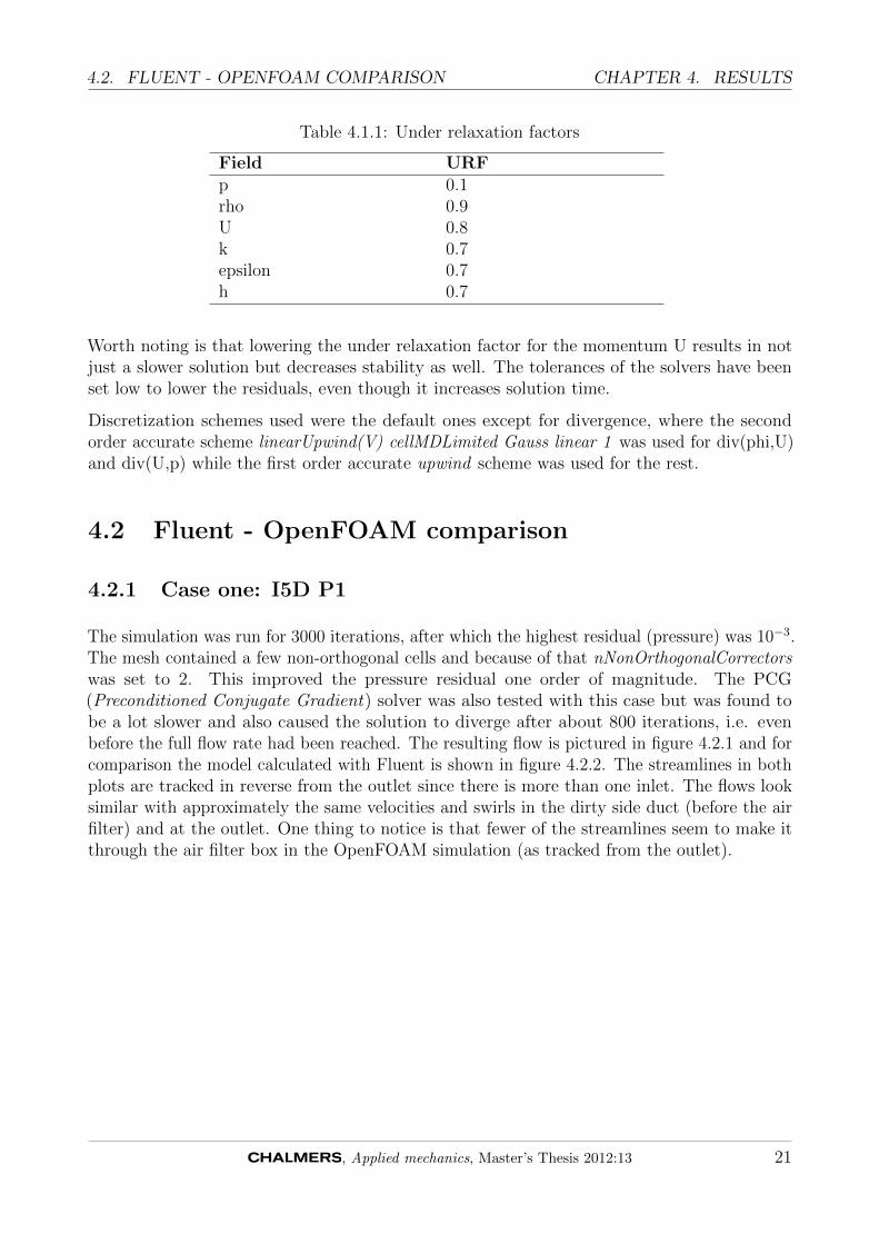
Field URFp 0.1rho 0.9U 0.8k 0.7epsilon 0.7h 0.7
Worth noting is that lowering the under relaxation factor for the momentum U results in notjust a slower solution but decreases stability as well. The tolerances of the solvers have beenset low to lower the residuals, even though it increases solution time.
Discretization schemes used were the default ones except for divergence, where the secondorder accurate scheme linearUpwind(V) cellMDLimited Gauss linear 1 was used for div(phi,U)and div(U,p) while the first order accurate upwind scheme was used for the rest.
4.2 Fluent - OpenFOAM comparison
4.2.1 Case one: I5D P1
The simulation was run for 3000 iterations, after which the highest residual (pressure) was 10−3.The mesh contained a few non-orthogonal cells and because of that nNonOrthogonalCorrectorswas set to 2. This improved the pressure residual one order of magnitude. The PCG(Preconditioned Conjugate Gradient) solver was also tested with this case but was found tobe a lot slower and also caused the solution to diverge after about 800 iterations, i.e. evenbefore the full flow rate had been reached. The resulting flow is pictured in figure 4.2.1 and forcomparison the model calculated with Fluent is shown in figure 4.2.2. The streamlines in bothplots are tracked in reverse from the outlet since there is more than one inlet. The flows looksimilar with approximately the same velocities and swirls in the dirty side duct (before the airfilter) and at the outlet. One thing to notice is that fewer of the streamlines seem to make itthrough the air filter box in the OpenFOAM simulation (as tracked from the outlet).
, Applied mechanics, Master’s Thesis 2012:13 21

4.2. FLUENT - OPENFOAM COMPARISON CHAPTER 4. RESULTS
Figure 4.2.1: Streamlines in the P1 system as calculated with OpenFOAM
Figure 4.2.2: Streamlines in the P1 system as calculated with Fluent
To study the pressure drop in more detail, the absolute values for total pressure drop fromthe inlet are presented in Table 4.2.1 together with corresponding values from Fluent. The
22 , Applied mechanics, Master’s Thesis 2012:13

4.2. FLUENT - OPENFOAM COMPARISON CHAPTER 4. RESULTS
pressure drop and uniformity index from OpenFOAM are calculated with the swak4foam scriptin Appendix B, while the Fluent values are calculated with built-in Fluent methods.
Table 4.2.1: Mass weighted average of total pressure drop (Pa)
Fluent OpenFOAM Differencesec2 entrance -893 -1248 39.8%sec3 dsd out -1623 -1662 2.4%sec4 filter inlet -2752 -2878 4.6%sec5 filter out -3115 -3165 1.6%sec6 amm in -3481 -3418 -1.8%sec7 csd1 in -4366 -4121 -5.6%sec8 csd2 in -5449 -5185 -4.8%sec9 outlet -5903 -5515 -6.6%
The first thing to note is that the OpenFOAM solver predicts the intake losses as a lothigher. This could be down to the difference in the way the boundary conditions are applied.OpenFOAM has been unable to achieve a stable solution with a negative mass flow on theoutlet, and instead the mass flow has been set at the inlets. When going downstream thepressure losses are much more similar in magnitude between the two softwares, and just afterthe filter OpenFOAM starts to predict a lower pressure loss than Fluent. That is, OpenFOAMpredicts a higher intake loss but a lower loss for the flow through the ducts. Figure 4.2.3 showsthe filter inlet velocity distribution for Fluent and OpenFOAM. The velocity distributions arerelatively similar but the solution from OpenFOAM is more chaotic in its nature. As will beshown later (section 4.2.3) OpenFOAM has problems with the velocities at the filter inlet.Even so, the correlation here is good compared to case two (figure 4.2.7). At the outlet (figure4.2.4) the velocity distributions are similar from both codes, as they should be.
Figure 4.2.3: Velocity distributions at the filter inlet in the P1 system with Fluent on the leftand OpenFOAM on the right
The uniformity indexes (table 4.2.2) are similar at the outlet and before the air mass meter,but the figure that stands out is at the filter inlet. This is not only a bad correlation to Fluent,which is not necessarily ”correct”, but the log files indicate that the uniformity index at the
, Applied mechanics, Master’s Thesis 2012:13 23

4.2. FLUENT - OPENFOAM COMPARISON CHAPTER 4. RESULTS
Figure 4.2.4: Velocity distributions at the outlet of the P1 system with Fluent on the left andOpenFOAM on the right
filter inlet varies between iterations. The other two uniformity indexes are constant, indicatingthat there is a problem with the velocity field at the filter inlet. This phenomenon is studiedin more detail in section 4.2.3.
Table 4.2.2: Area weighted uniformity index
Fluent OpenFOAM Differencesec4 filter inlet 0.763 0.854 11.9%sec6 amm in 0.924 0.948 2.6%sec9 outlet 0.869 0.854 -1.7%
4.2.2 Case two: I5D EuCD
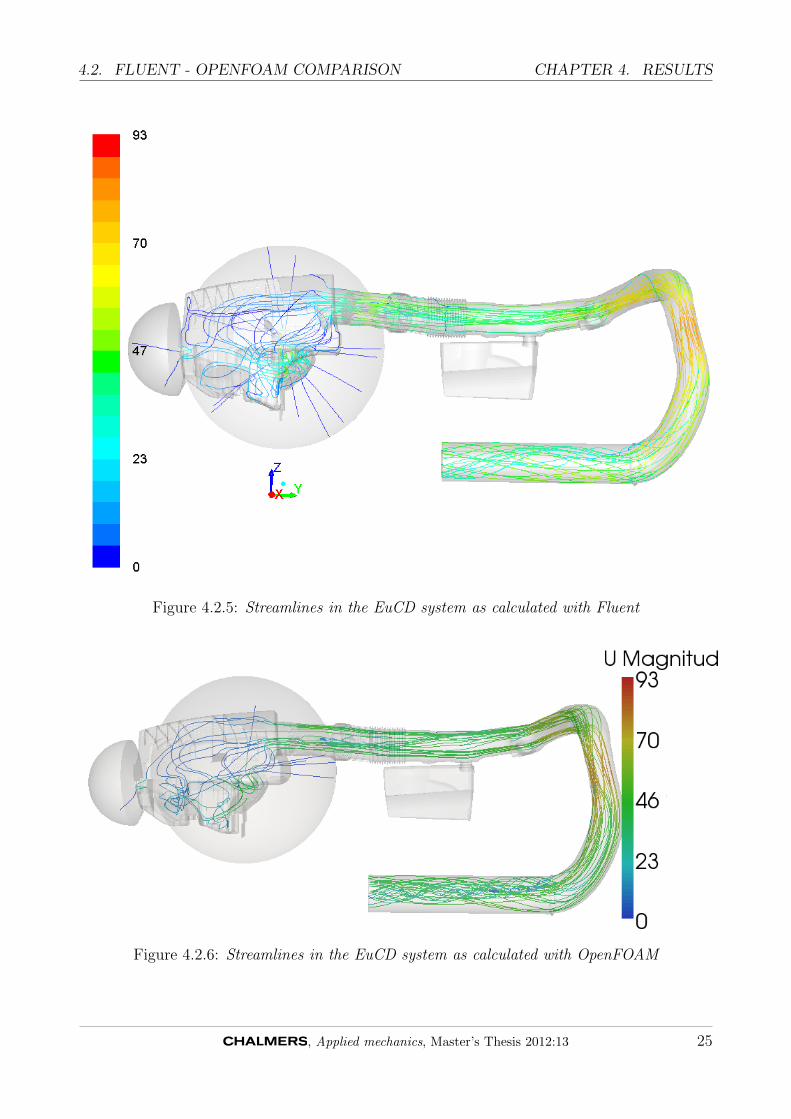
The geometry of case two is simpler than that of case one with no duct connecting inlet two tothe air filter box and a shorter duct from inlet 1. With the same level of mesh refinement thisled to a shorter solution time of just under 2 hours for the same amount of iterations as in caseone. As in case one the highest residual (pressure) was in the region of 10−3. Also in this caseboth softwares capture the outlet swirl in the same way (figures 4.2.5 and 4.2.6). Interesting tonote is that in this case as well a smaller part of the streamlines (tracked in reverse direction)seem to make it past the air filter. The reason for this is unknown, but could be related to thephenomenon described in section 4.2.3.
24 , Applied mechanics, Master’s Thesis 2012:13
4.2. FLUENT - OPENFOAM COMPARISON CHAPTER 4. RESULTS
Figure 4.2.5: Streamlines in the EuCD system as calculated with Fluent
Figure 4.2.6: Streamlines in the EuCD system as calculated with OpenFOAM
, Applied mechanics, Master’s Thesis 2012:13 25
4.2. FLUENT - OPENFOAM COMPARISON CHAPTER 4. RESULTS
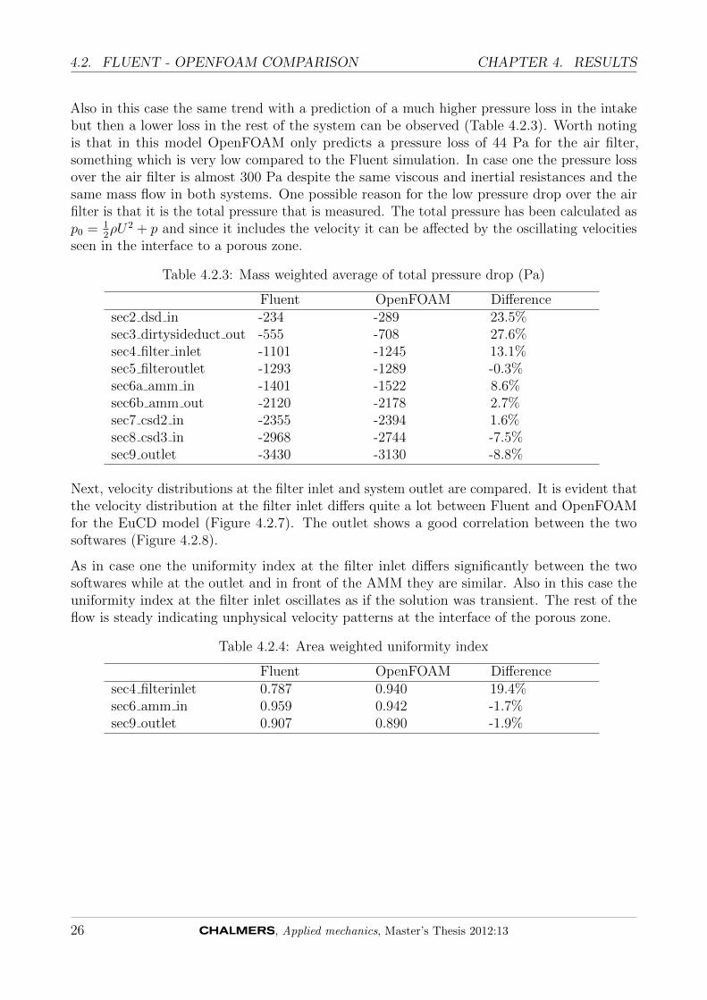
Also in this case the same trend with a prediction of a much higher pressure loss in the intakebut then a lower loss in the rest of the system can be observed (Table 4.2.3). Worth notingis that in this model OpenFOAM only predicts a pressure loss of 44 Pa for the air filter,something which is very low compared to the Fluent simulation. In case one the pressure lossover the air filter is almost 300 Pa despite the same viscous and inertial resistances and thesame mass flow in both systems. One possible reason for the low pressure drop over the airfilter is that it is the total pressure that is measured. The total pressure has been calculated asp0 = 1
2ρU2 + p and since it includes the velocity it can be affected by the oscillating velocities
seen in the interface to a porous zone.
Table 4.2.3: Mass weighted average of total pressure drop (Pa)
Fluent OpenFOAM Differencesec2 dsd in -234 -289 23.5%sec3 dirtysideduct out -555 -708 27.6%sec4 filter inlet -1101 -1245 13.1%sec5 filteroutlet -1293 -1289 -0.3%sec6a amm in -1401 -1522 8.6%sec6b amm out -2120 -2178 2.7%sec7 csd2 in -2355 -2394 1.6%sec8 csd3 in -2968 -2744 -7.5%sec9 outlet -3430 -3130 -8.8%
Next, velocity distributions at the filter inlet and system outlet are compared. It is evident thatthe velocity distribution at the filter inlet differs quite a lot between Fluent and OpenFOAMfor the EuCD model (Figure 4.2.7). The outlet shows a good correlation between the twosoftwares (Figure 4.2.8).
As in case one the uniformity index at the filter inlet differs significantly between the twosoftwares while at the outlet and in front of the AMM they are similar. Also in this case theuniformity index at the filter inlet oscillates as if the solution was transient. The rest of theflow is steady indicating unphysical velocity patterns at the interface of the porous zone.
Table 4.2.4: Area weighted uniformity index
Fluent OpenFOAM Differencesec4 filterinlet 0.787 0.940 19.4%sec6 amm in 0.959 0.942 -1.7%sec9 outlet 0.907 0.890 -1.9%
26 , Applied mechanics, Master’s Thesis 2012:13

4.2. FLUENT - OPENFOAM COMPARISON CHAPTER 4. RESULTS
Figure 4.2.7: Velocity distributions at the filter inlet in the EuCD system with Fluent on theleft and OpenFOAM on the right
Figure 4.2.8: Velocity distributions at the outlet of the EuCD system with Fluent on the leftand OpenFOAM on the right
, Applied mechanics, Master’s Thesis 2012:13 27
4.2. FLUENT - OPENFOAM COMPARISON CHAPTER 4. RESULTS
4.2.3 Oscillating velocity at porous interface
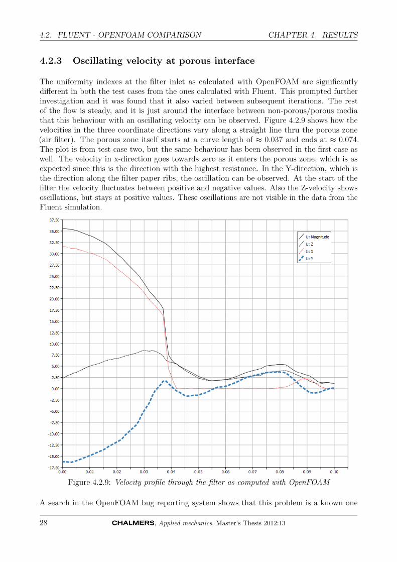
The uniformity indexes at the filter inlet as calculated with OpenFOAM are significantlydifferent in both the test cases from the ones calculated with Fluent. This prompted furtherinvestigation and it was found that it also varied between subsequent iterations. The restof the flow is steady, and it is just around the interface between non-porous/porous mediathat this behaviour with an oscillating velocity can be observed. Figure 4.2.9 shows how thevelocities in the three coordinate directions vary along a straight line thru the porous zone(air filter). The porous zone itself starts at a curve length of ≈ 0.037 and ends at ≈ 0.074.The plot is from test case two, but the same behaviour has been observed in the first case aswell. The velocity in x-direction goes towards zero as it enters the porous zone, which is asexpected since this is the direction with the highest resistance. In the Y-direction, which isthe direction along the filter paper ribs, the oscillation can be observed. At the start of thefilter the velocity fluctuates between positive and negative values. Also the Z-velocity showsoscillations, but stays at positive values. These oscillations are not visible in the data from theFluent simulation.
Figure 4.2.9: Velocity profile through the filter as computed with OpenFOAM
A search in the OpenFOAM bug reporting system shows that this problem is a known one
28 , Applied mechanics, Master’s Thesis 2012:13

4.3. VALIDATION WITH EXPERIMENTS CHAPTER 4. RESULTS
[11]. In the bug report there is also a suggested fix. It consists of replacing the line ofcode U -= rUA*fvc::grad(p) for U = fvc::reconstruct(phi)/rho in the pEqn.H file used in therhoPorousMRFSimpleFoam source file. This change was made and the solver recompiled.Although this is somewhat outside of the scope set up in the limitations (section 1.3) it wasdeemed important for the conclusions to evaluate the fix. Both of the test cases were run againwith the new solver but otherwise identical settings. The results were similar to the originalsolver and the velocity patterns remained unphysical and changing on every iteration at thestart of the porous zone.
4.3 Validation with experiments
Total pressure drops over the systems as measured from experiments are presented in Table4.3.1. For these cases the OpenFOAM simulations are further from the experimental results.In the P1 case OpenFOAM is off by 9% and in the EuCD case by a substantial 25%, comparedto 2 and 18% for Fluent. The measurements in the flow rig are taken by a pressure sensormounted between the outlet and the attachment to flow rig, visible in figure 3.2.5. One thingto have in mind during this comparison is that OpenFOAM could not be made to run withthe flow set at the outlet, and even though the mass flows through the systems are the same,the boundary conditions are not identical.
Table 4.3.1: Total pressure drop computed from CFD simulations and measurements (Pa)
Case OpenFOAM Fluent ExperimentP1 5515 5903 6052EuCD 3130 3430 4177
4.4 Parallel scaling
Since CFD is very demanding with respect to computing power, it is important to use theoptimal number of processors/cores when doing an analysis utilising parallel computing. Thisis important both in respect to shortening lead times in development projects and to use theavailable computing resources as efficiently as possible. OpenFOAM uses domain decompositionfor processing in parallel. This means that the geometry and associated fields are dividedinto parts for each processor/core going to be used for the computation. To determine theoptimal number of cores to use when running cases in parallel, a test has been conducted bysolving the same case using a varying amount of cores. The model used is similar to the testcases and consists of 6 million cells. This is a typical size for air induction system models.The type of simulation is the same as in the test cases, i.e. steady state, compressible withrealizable k-epsilon turbulence model and porous media for the filter. To obtain a simulationtime, the case was run for 2000 iterations and the clocktime read from the log file. The casewas run with 16,32,48,64,96,128,144,160,172,192, 256 and 384 cores. The number of cores usedis only relevant for a case with around the same number of cells as the one used in this test.Instead, the average number of cells per core has been used as a measure to help decide the
, Applied mechanics, Master’s Thesis 2012:13 29

4.5. TOPOLOGY OPTIMISATION CHAPTER 4. RESULTS
optimum number of cores for any given case. Presented in figure 4.4.1, the conclusion is thatthe optimum lies around 50000 cells per core used. With more cells than this per core theinterconnections aren’t saturated and so more cores equals shorter solution time. And withfewer cells per core, the interconnections between the cores/nodes become the bottleneck andthis might actually lead to a slower calculation.
Figure 4.4.1: Number of cells/core for optimum computing performance
4.5 Topology optimisation
To achieve convergence with the adjoint solver proved to be difficult, but after raising thevalue alphaMax to 106, which corresponds to the maximum porosity in the blocked cells, asatisfactory level of convergence was achieved with the highest residual in the region of 10−4.The obtained geometry is shown in figure 4.5.1. The new geometry created in the box resemblesthe shape of a circular duct, but with a varying radius. The rough edges seen in the newgeometry are the individual cells that have been blocked.
The flow changed significantly between the unmodified and adjoint optimised design space.Figure 4.5.2 shows streamlines for both the modified and unmodified geometry. The optimisedgeometry removes all of the large scale swirl and this should lower the pressure drop. However,the total pressure drop from inlet to outlet was about the same for both geometries. Since thesolver is supposed to optimise with respect to lowering pressure loss, this was unexpected. Onereason for the pressure drop not being lower in the modified design could be because of therough walls created by the blocked cells. The mesh used here had approximately 300000 cells.To try and lower the effect of the rough edges a refined mesh with 800000 cells was tested as
30 , Applied mechanics, Master’s Thesis 2012:13

4.5. TOPOLOGY OPTIMISATION CHAPTER 4. RESULTS
Figure 4.5.1: Geometry obtained after adjoint optimisation
well. The results were still the same and it was concluded that if the rough cell edges wereresponsible for the pressure drop being unchanged before and after optimisation, refining themesh does not help. To get the real benefit of an adjoint optimisation with blocked cells therough surface obtained would probably have to be imported into the CAD model and used asa guide when updating the design.
Figure 4.5.2: Streamlines for original and optimised geometries
, Applied mechanics, Master’s Thesis 2012:13 31
CHAPTER 5. DISCUSSION AND CONCLUSIONS
5 Discussion and conclusions
The most important part of this work has been to assess whether OpenFOAM can be usedas a tool to reliably predict the flow in automotive air induction systems. Also part of thethesis has been to investigate the possibilities and suitability of using OpenFOAM as a tool inoptimising the shape of future air induction systems.
5.1 System simulations
Comparing the results from Fluent and OpenFOAM simulations it is evident that there aresome differences between the softwares. The absolute numbers on pressure loss obtained withOpenFOAM were further from the experimental values than the ones obtained with Fluent.OpenFOAM simulations show a pressure drop almost 10% lower than the simulation fromFluent. The problem here is that already Fluent tends to under predict the losses compared toexperimental results. There are also differences in where the losses take place in the system.Fluent shows a higher loss in the ducts compared to OpenFOAM, while the latter shows ahigher loss in the intake. It is hard to tell exactly where these differences come from, but itshould be noted that the same numerical settings and boundary conditions have not beenpossible to use. OpenFOAM couldn’t handle the flow being prescribed at the outlet, but insteadit had to be set at the inlets. If the same boundary conditions would have been possible to usein experiments and simulations they could have been validated in more thorough way againsteach other. The simulations involving porous zones turned out to be highly unstable. Despiteseveral initiation techniques such as starting with incompressible flow, 1st order numericalschemes and low flow speeds the OpenFOAM simulations couldn’t be made to use all secondorder schemes for the numerics. This will of course affect the results, but at least the mostimportant field (momentum) could be run with a second order scheme. The tolerances of thelinear solvers were set to low values. This increased solution time but was necessary to achievereasonably low residuals. Even with the low tolerances, OpenFOAM had a speed advantagecompared to Fluent.
The work carried out when writing this thesis has included testing a great number of combina-tions of URFs, numerical schemes and solver settings. Even so, it can not be ruled out thatfurther tests and trials could find settings that can be used to better predict the air inductionsystem flows. There is also the problem encountered with the oscillating flow speeds in thetransition to a porous zone (the air filter). As no solution to this is presently known this mustbe considered a drawback for OpenFOAM when simulating complete air filter systems. Even ifthis phenomenon does not affect the pressure loss over the whole system in a significant way, itmakes the uniformity index at the filter inlet useless. When simulating single ducts without anair filter there are no problems in using all second order numerical schemes, further indicatingthat it is the porous media implementation that suffers from a problem. In post-processing,the total pressure drop and uniformity indexes can easily be read in the log-file with the useof swak4foam. This is an advantage compared to Fluent as no post-processing is needed (orrather post-processing is done on-the-fly). OpenFOAM data can easily be converted to mostpost-processing software formats. It should be noted though that the conversion isn’t optimal
32 , Applied mechanics, Master’s Thesis 2012:13

5.2. TOPOLOGY OPTIMISATION CHAPTER 5. DISCUSSION AND CONCLUSIONS
as data from internal surfaces doesn’t follow. The only way found to present plots of thedata on internal surfaces such as figure 4.2.3 is to use the paraFoam wrapper for Paraview.One of the greatest advantages with OpenFOAM is that it is command-line based. Thismakes it easy to automatise and integrate with other softwares. Outside of the scope of thisthesis, but nevertheless also significant merit for OpenFOAM is the possibility for users to addfunctionality.
The parallel scalability with regard to number of cores used does depend on certain variablessuch as the geometry of the mesh, the decomposition method used and resulting number ofshared interfaces between processors. The main reason for the scalability not being linear isusually that the processors and nodes have to shuffle a lot of data between each other and thememory (depending on the number of shared faces). The speed of the interfaces between nodesand processors are one of the most important variables when considering the effectiveness inincreasing the number of cores to use for a simulation. The test conducted reflects the optimalwith the current setup used at VCC.
This thesis has shown that there are problems in simulating the air filter systems withOpenFOAM, the most severe being the oscillating velocities at the porous interface (see section4.2.3). If a solution to this is found there are no substantial obstacles for using OpenFOAM asthe main CFD-package for the air induction systems.
5.2 Topology Optimisation
When optimising the absolute numbers are not as important as long as the differences withchanging geometry are correct. OpenFOAM is command-line based and this makes it very easyto integrate with optimisation softwares such as modeFrontier. Together with the fact that itis free [5] and thus lowering the licensing costs for simulation runs this makes OpenFOAM verysuitable to use for DOE-based optimisation loops. The integrated pre- and post-processingsuch as the swak4foam script used in this thesis is also very useful in an optimisation loop as itenables extraction of a wide variety of data without user interaction.
The adjoint solver currently distributed with OpenFOAM (version 2.1.0) is a very basic solver.The solver optimises against one variable, total pressure loss. It also changes the geometryby adding blockages to the cells that contribute to pressure loss as suggested by the adjointequations. While this works well to get an idea of where the losses occur, the geometry achievedwith the blocked cells is less than optimal in the sense that it creates very rough walls. It ispossible to extract this surface and use it as input in CAD software when improving a design.A better approach for changing the geometry would probably be to use some kind of CADparametrisation or mesh morphing to get an optimised model directly.
Another thing to take into consideration with the adjoint method is that it does not take otherfactors such as manufacturability and manufacturing cost into account when computing theoptimal shape. This can create good geometries with respect to the optimised variable, butwhich are not possible to manufacture. The result will therefore always require at least someinterpretation by a designer before it can be used. For this reason the results obtained from anadjoint method optimisation are best suited as a guide to where changes need to be made in adesign rather than using the geometry directly. A conclusion regarding the adjoint method
, Applied mechanics, Master’s Thesis 2012:13 33

5.2. TOPOLOGY OPTIMISATION CHAPTER 5. DISCUSSION AND CONCLUSIONS
for optimising air induction system topologies is that it is a good tool to use for a designerin determining where to make changes. But it is not a tool producing a geometry ready forproduction.
34 , Applied mechanics, Master’s Thesis 2012:13

CHAPTER 6. RECOMMENDATIONS FOR FURTHER WORK
6 Recommendations for further work
• Even though time consuming, continued investigations into finding numerical schemesetc. could possibly improve the performance and stability when using OpenFOAM forsimulating complete air filter systems.
• Finding a solution to the porous boundary problem would enable OpenFOAM to be usedin predicting filter utilisation, something which is now not possible.
• While the adjoint method holds great potential the solver currently distributed withOpenFOAM is of a very simple nature. To improve the usability of the adjoint method anew solver would have to be developed. On the wish list for a new solver would be, forexample, the ability to handle compressible flows, more variables to optimise against (forexample uniformity index) and to only apply the adjoint equations to certain parts ofthe mesh, for example a cellZone.
• Investigate the OpenFOAM meshing tool snappyHexMesh for meshing the air inductionsystems.
, Applied mechanics, Master’s Thesis 2012:13 35

REFERENCES
References
[1] F. M. White. Fluid Mechanics. Sixth Edition. McGraw-Hill, 2008.[2] A. N. Kolmogorov. “Equation of turbulent motion of an incompressible fluid.” In: Physics
6 (1941), pp. 56–58.[3] W. P. Jones and B. E. Launder. “The prediction of laminarization with a two-equation
model of turbulence.” In: International Journal of Heat and Mass Transfer 15 (1972),pp. 301–314.
[4] H. K. Versteeg and W Malalasekera. An Introduction to Computational Fluid Dynamics,The Finite Volmue Method. Second Edition. Pearson Education, 2007.
[5] GNU General Public License. Version 3. 2007. url: http://www.gnu.org/licenses/gpl.html.
[6] OpenFOAM Userguide. Version 2.1. OpenCFD, 2011. url: http://www.openfoam.org/docs/user/.
[7] H. E. Hafsteinsson. “Porous Media in OpenFOAM”. 2009.[8] M. Dybeck. “CFD-procedures for Air Induction Systems”. MA thesis. Lulea University
of Technology, 2011.[9] R. Schneider. “Applications of the Discrete Adjoint Method in Computational Fluid
Dynamics”. PhD thesis. University of Leeds, 2006.[10] C. Hinterberger and M. Olesen. “Industrial application of continuous adjoint flow solvers
for the optimization of automotive exhaust systems”. In: ECCOMAS. 2011.[11] 0000134: Unphysical velocity patterns at the interface of a porous zone. 2011. url:
http://www.openfoam.org/mantisbt/view.php?id=134.
36 , Applied mechanics, Master’s Thesis 2012:13

APPENDIX A. INTRODUCTION TO OPENFOAM
A Introduction to OpenFOAM
OpenFOAM is an abbreviation which stands for ”Open source Field Operation And Manipula-tion” and is an open source numerical simulation software with extensive capabilities in solvingfluid flows and other multi-physics problems. From the beginning (circa 1993) the softwarewas called simply FOAM and was first developed as part of a PhD project at Imperial CollegeLondon. In 2004 it became open source under the GNU GPL license [5] and changed name toOpenFOAM. Today it is developed by SGI R© and widely used by both academic institutionsand corporations worldwide.
The OpenFOAM distribution includes a lot of things, but the basis is the C++ libraries.The libraries contain the OpenFOAM classes which are designed to make it easier to writeapplications that solve continuum mechanics problems. Even though you still need someprogramming knowledge, a thorough knowledge of C++ is not a hard requirement to createor edit OpenFOAM applications. The classes provide a syntax which resembles the originalequation. This example from the OpenFOAM userguide [6] is probably one of the simpler onesbut shows the idea behind the OpenFOAM classes. The equation A.0.1
∂ρU
∂t+∇ • φU−∇ • µ∇U = −∇p (A.0.1)
is in OpenFOAM represented by the code:
s o l v e(
fvm : : ddt ( rho , U)+ fvm : : div ( phi , U)− fvm : : l a p l a c i a n (mu, U)
==− f v c : : grad (p)
) ;
The OpenFOAM distribution includes a large number of solvers. Each solver is designed to solvea specific type of problem. Most are designed to solve some kind of CFD problem but there arealso solvers for other types of problems such as electro magnetic and financial problems. Theother type of application distributed with OpenFOAM are the utilities. They handle mostlypre- and post-processing functions such as mesh conversion and data manipulation.
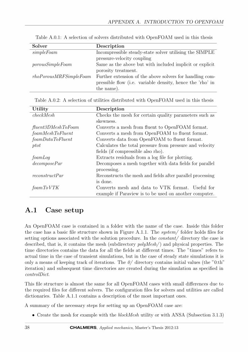
Table A.0.1 and Table A.0.2 contains a selection of solvers and utilities that are part of theOpenFOAM distribution and have been used in this thesis.
, Applied mechanics, Master’s Thesis 2012:13 37
APPENDIX A. INTRODUCTION TO OPENFOAM
Table A.0.1: A selection of solvers distributed with OpenFOAM used in this thesis
Solver DescriptionsimpleFoam Incompressible steady-state solver utilising the SIMPLE
pressure-velocity couplingporousSimpleFoam Same as the above but with included implicit or explicit
porosity treatment.rhoPorousMRFSimpleFoam Further extension of the above solvers for handling com-
pressible flow (i.e. variable density, hence the ’rho’ inthe name).
Table A.0.2: A selection of utilities distributed with OpenFOAM used in this thesis
Utility DescriptioncheckMesh Checks the mesh for certain quality parameters such as
skewness.fluent3DMeshToFoam Converts a mesh from fluent to OpenFOAM format.foamMeshToFluent Converts a mesh from OpenFOAM to fluent format.foamDataToFluent Converts data from OpenFOAM to fluent format.ptot Calculates the total pressure from pressure and velocity
fields (if compressible also rho).foamLog Extracts residuals from a log file for plotting.decomposePar Decomposes a mesh together with data fields for parallel
processing.reconstructPar Reconstructs the mesh and fields after parallel processing
is done.foamToVTK Converts mesh and data to VTK format. Useful for
example if Paraview is to be used on another computer.
A.1 Case setup
An OpenFOAM case is contained in a folder with the name of the case. Inside this folderthe case has a basic file structure shown in Figure A.1.1. The system/ folder holds files forsetting options associated with the solution procedure. In the constant/ directory the case isdescribed, that is, it contains the mesh (subdirectory polyMesh/ ) and physical properties. Thetime directories contains the data for all the fields at different times. The ”times” refers toactual time in the case of transient simulations, but in the case of steady state simulations it isonly a means of keeping track of iterations. The 0/ directory contains initial values (the ”0:th”iteration) and subsequent time directories are created during the simulation as specified incontrolDict.
This file structure is almost the same for all OpenFOAM cases with small differences due tothe required files for different solvers. The configuration files for solvers and utilities are calleddictionaries. Table A.1.1 contains a description of the most important ones.
A summary of the necessary steps for setting up an OpenFOAM case are:
• Create the mesh for example with the blockMesh utility or with ANSA (Subsection 3.1.3)
38 , Applied mechanics, Master’s Thesis 2012:13

APPENDIX A. INTRODUCTION TO OPENFOAM
Figure A.1.1: Directory structure of an OpenFOAM case
Table A.1.1: Description of the most important OpenFOAM dictionaries used in this thesis
Dictionary DescriptioncontrolDict Controls start/stop, iterations, data writing and also
contains function objects. Function objects are pieces ofcode that runs on every iteration.
fvSolution Specifies the types of linear solvers, algorithms and underrelaxation factors to use.
fvSchemes Specifies numerical schemes.boundary Sets boundary types.transportProperties Defines fluid properties for incompressible solvers.thermophysicalProperties Specifies thermophysical properties of a fluid when using
the energy equation (with compressible solvers).RASProperties Specifies RAS turbulence model, cf. LES modelling.decomposeParDict Options for the mesh decomposition required for parallel
computing.
or convert the mesh from another format with a utility such as fluent3DMeshToFoam.
• Set boundary types in the polyMesh/boundary dictionary. In this thesis patch has beenused for inlets/outlets etc and wall for walls.
• Set boundary conditions in the 0/ directory. Depending on the method used to createthe mesh, it may be necessary to create/edit the volume field dictionaries manually.
• Set turbulence model in RASProperties/LESProperties dictionary for turbulent simula-tions.
• Set fluid properties such as µ and cp. For most solvers this is done in either transport-
, Applied mechanics, Master’s Thesis 2012:13 39

APPENDIX A. INTRODUCTION TO OPENFOAM
Properties or thermophysicalProperties.
• Set solution algorithms in fvSolution dictionary.
• Set schemes in fvSchemes dictionary.
• Set simulation controls in the controlDict dictionary.
• Decompose the case with decomposePar if using more than one core for solving.
When all the settings are set to appropriate values, the solver of choice is started by runningthe solver from the case directory. For parallel processing, the process of starting the solverdepends on the type of parallel processing/queuing system used.
40 , Applied mechanics, Master’s Thesis 2012:13

APPENDIX B. SWAK4FOAM SCRIPT
B swak4foam script
Below are examples of the entries used to calculate total pressure and uniformity index on theinterior sections, in OpenFOAM defined as faceZones. Last is the code used to display massflows on the inlets and outlet.
Entry for calculating the total pressure on a faceZone (mass weighted average)
Total−p r e s s u r e s e c 9 o u t l e t{
func t i onObjec tL ibs (” l ibs impleSwakFunct ionObjects . so ” ) ;
type swakExpression ;outputControl outputTime ;valueType faceZone ;zoneName s e c 9 o u t l e t ;e xp r e s s i on”sum ( ( 0 . 5∗ rho∗pow(mag(U) ,2)+p )∗ ( area ( )∗ rho ) )/(sum( area ( )∗ rho ) ) ” ;
accumulat ions(
average) ;verbose t rue ;a u t o I n t e r p o l a t e t rue ;warnAutoInterpolate f a l s e ;
}
Entry for calculating the uniformity index on a faceZone (area weighted average)
U I s e c 9 o u t l e t{
type swakExpression ;outputControl t imeStep ;valueType faceZone ;zoneName s e c 9 o u t l e t ;accumulat ions(
max) ;exp r e s s i on”1−sum ( ( s q r t (pow ( ( average (mag(U))−mag(U) ) , 2 ) ) /(2∗sum( area ( ) )∗ average (mag(U) ) ) ) ∗ area ( ) ) ” ;
verbose t rue ;a u t o I n t e r p o l a t e t rue ;
, Applied mechanics, Master’s Thesis 2012:13 41

APPENDIX B. SWAK4FOAM SCRIPT
warnAutoInterpolate f a l s e ;}
Entry for printing mass flows across the boundaries
massFlow{
func t i onObjec tL ibs (” l ibs impleSwakFunct ionObjects . so ” ) ;type patchMassFlow ;verbose t rue ;patches(
i n l e t 1i n l e t 2p r e s s u r e o u t l e t
) ;f a c t o r 1 ;
}
42 , Applied mechanics, Master’s Thesis 2012:13

APPENDIX C. PYTHON SCRIPT
C Python script
Python script for automation of the solving process. It changes from incompressible tocompressible simulation settings and switches divergence schemes. Uses the Python libraryPyFoam.
#!/ usr / bin /python
import os , sys , s h u t i l
from PyFoam . App l i ca t i on s . Decomposer import Decomposerfrom PyFoam . App l i ca t i on s . Runner import Runnerfrom PyFoam . App l i ca t i on s . PlotRunner import PlotRunnerfrom PyFoam . Execution . BasicRunner import BasicRunner
case=sys . argv [ 1 ]proc=i n t ( sys . argv [ 2 ] ) #number o f c o r e si t e incomp=i n t ( sys . argv [ 3 ] ) #number o f i t e r a t i o n s f o r i n compre s s i b l e
#Schemes to use f o r d ive rgence ( in order o f use )divSchemesV=[ ’ upwind ’ , ’ linearUpwindV ’ ] ;divSchemes=[ ’ upwind ’ , ’ l inearUpwind ’ ] ;
#s o l v e r s to useso lver incomp=”porousSimpleFoam”solver comp=”rhoPorousMRFSimpleFoam”
# Set t i ng a p p l i c a t i o n to porousSimpleFoampr in t ’\ nSet t ing a p p l i c a t i o n to porousSimpleFoam ’
in f i l ename=’%s / system/ cont ro lD ic t ’ %caseout f i l ename=’%s / system/controlDictTemp ’ %casei f i l e = open ( in f i l ename , ’ r ’ )o f i l e = open ( out f i l ename , ’w’ )l i n e s = i f i l e . r e a d l i n e s ( )
f o r l i n e in l i n e s :words = l i n e . s p l i t ( )f o r word in words :
index = words . index ( word )i f word == ’ app l i c a t i on ’ :
words [ index +1] = so lver incomp + ’; ’cont inue
newl ine =’ ’ . j o i n ( words )o f i l e . wr i t e ( ’% s\n ’ % newl ine )
i f i l e . c l o s e ( )
, Applied mechanics, Master’s Thesis 2012:13 43

APPENDIX C. PYTHON SCRIPT
o f i l e . c l o s e ( )os . remove ( i n f i l ename )os . rename ( out f i l ename , i n f i l ename )
#Decompose f o r g iven number o f c o r e sDecomposer ( args=[”−−prog r e s s ”,”−−method=scotch ” , case , s t r ( proc ) ] )
#Set the divScheme to Gauss upwind ; ( f i r s t order accurate )#s h u t i l . copy ( ’% s / system/ fvSchemes ’% case , ’% s / system/ fvSchemes . old ’% case )#pr in t ’\ nSet t ing divScheme to Gauss %s f o r Momentum, k , eps , h and pres sure ’ % ’ ’ . j o i n (map( s t r , divSchemes [ 0 ] ) )
#in f i l ename=’%s / system/ fvSchemes ’ %case#out f i l ename=’%s / system/fvSchemesTemp ’ %case#i f i l e = open ( in f i l ename , ’ r ’ )#o f i l e = open ( out f i l ename , ’w’ )#l i n e s = i f i l e . r e a d l i n e s ( )##f o r l i n e in l i n e s :# words = l i n e . s p l i t ( )# f o r word in words :# index = words . index ( word )# i f word == ’ div ( phi ,U) ’ :# words [ index +2] = divSchemesV [ 0 ] + ’ ; ’# cont inue# i f word == ’ div ( phi , k ) ’ :# words [ index +2] = divSchemes [ 0 ] + ’ ; ’# cont inue# i f word == ’ div ( phi , e p s i l o n ) ’ :# words [ index +2] = divSchemes [ 0 ] + ’ ; ’# cont inue# i f word == ’ div ( phi , h ) ’ :# words [ index +2] = divSchemes [ 0 ] + ’ ; ’# cont inue# i f word == ’ div (U, p ) ’ :# words [ index +2] = divSchemes [ 0 ] + ’ ; ’# cont inue# newl ine =’ ’ . j o i n ( words )# o f i l e . wr i t e ( ’% s\n ’ % newl ine )#i f i l e . c l o s e ( )#o f i l e . c l o s e ( )#os . remove ( i n f i l ename )#os . rename ( out f i l ename , i n f i l ename )
#Run s o l v e r with in compre s s i b l e s o l v e rp r i n t ’\nRunning 500 i t e r a t i o n s with %s ’ %so lver incompRunner ( args=[”−−proc=%d”%proc ,”−−prog r e s s ” , so lver incomp ,”− case ” , case ] )
44 , Applied mechanics, Master’s Thesis 2012:13

APPENDIX C. PYTHON SCRIPT
#Reconstruct the case to be ab le to manipulate f i e l d sRunner ( args =[” recons t ruc tPar ”,”− case ” , case ] )
#change to compres s ib l e s e t t i n g s#(p and phi dimensions , c o n t r o l d i c t , k & e p s i l o n wa l l f u n c t i o n s )p r i n t ’\ nSwitching to compres s ib l e s o l v e r s e t t i n g s ’
#k wallFin f i l ename=’%s /500/k ’ %caseout f i l ename=’%s /500/kTemp ’ %casei f i l e = open ( in f i l ename , ’ r ’ )o f i l e = open ( out f i l ename , ’w’ )l i n e s = i f i l e . r e a d l i n e s ( )
f o r l i n e in l i n e s :l i n e = l i n e . r e p l a c e (” kqRWallFunction ” ,” compres s ib l e : : kqRWallFunction ”)o f i l e . wr i t e ( l i n e )
i f i l e . c l o s e ( )o f i l e . c l o s e ( )os . remove ( i n f i l ename )os . rename ( out f i l ename , i n f i l ename )
#eps wallFin f i l ename=’%s /500/ eps i l on ’ %caseout f i l ename=’%s /500/ epsilonTemp ’ %casei f i l e = open ( in f i l ename , ’ r ’ )o f i l e = open ( out f i l ename , ’w’ )l i n e s = i f i l e . r e a d l i n e s ( )
f o r l i n e in l i n e s :l i n e = l i n e . r e p l a c e (” eps i lonWal lFunct ion ” ,” compre s s ib l e : : eps i lonWal lFunct ion ”)o f i l e . wr i t e ( l i n e )
i f i l e . c l o s e ( )o f i l e . c l o s e ( )os . remove ( i n f i l ename )os . rename ( out f i l ename , i n f i l ename )
#eps i n l e ti n f i l ename=’%s /500/ eps i l on ’ %caseout f i l ename=’%s /500/ epsilonTemp ’ %casei f i l e = open ( in f i l ename , ’ r ’ )o f i l e = open ( out f i l ename , ’w’ )l i n e s = i f i l e . r e a d l i n e s ( )
f o r l i n e in l i n e s :
, Applied mechanics, Master’s Thesis 2012:13 45
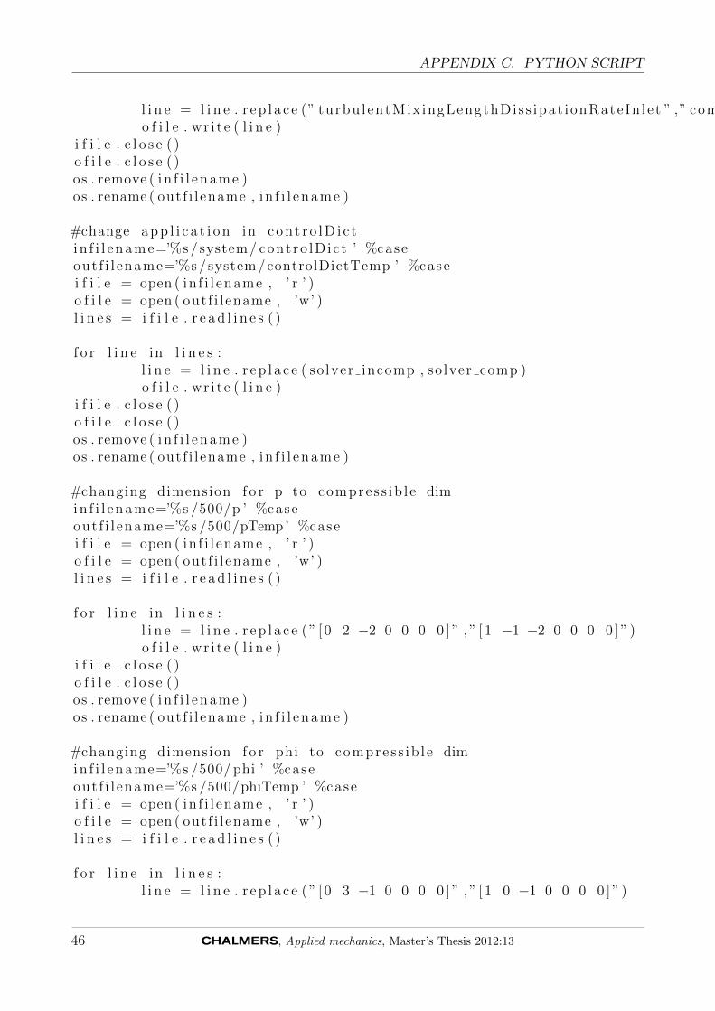
APPENDIX C. PYTHON SCRIPT
l i n e = l i n e . r e p l a c e (” turbu l entMix ingLengthDi s s ipat i onRate In l e t ” ,” compre s s ib l e : : tu rbu l entMix ingLengthDi s s ipat i onRate In l e t ”)o f i l e . wr i t e ( l i n e )
i f i l e . c l o s e ( )o f i l e . c l o s e ( )os . remove ( i n f i l ename )os . rename ( out f i l ename , i n f i l ename )
#change a p p l i c a t i o n in c on t r o lD i c ti n f i l ename=’%s / system/ cont ro lD ic t ’ %caseout f i l ename=’%s / system/controlDictTemp ’ %casei f i l e = open ( in f i l ename , ’ r ’ )o f i l e = open ( out f i l ename , ’w’ )l i n e s = i f i l e . r e a d l i n e s ( )
f o r l i n e in l i n e s :l i n e = l i n e . r e p l a c e ( so lver incomp , so lver comp )o f i l e . wr i t e ( l i n e )
i f i l e . c l o s e ( )o f i l e . c l o s e ( )os . remove ( i n f i l ename )os . rename ( out f i l ename , i n f i l ename )
#changing dimension f o r p to compres s ib l e dimin f i l ename=’%s /500/p ’ %caseout f i l ename=’%s /500/pTemp’ %casei f i l e = open ( in f i l ename , ’ r ’ )o f i l e = open ( out f i l ename , ’w’ )l i n e s = i f i l e . r e a d l i n e s ( )
f o r l i n e in l i n e s :l i n e = l i n e . r e p l a c e ( ” [ 0 2 −2 0 0 0 0 ] ” , ” [ 1 −1 −2 0 0 0 0 ] ” )o f i l e . wr i t e ( l i n e )
i f i l e . c l o s e ( )o f i l e . c l o s e ( )os . remove ( i n f i l ename )os . rename ( out f i l ename , i n f i l ename )
#changing dimension f o r phi to compres s ib l e dimin f i l ename=’%s /500/ phi ’ %caseout f i l ename=’%s /500/phiTemp ’ %casei f i l e = open ( in f i l ename , ’ r ’ )o f i l e = open ( out f i l ename , ’w’ )l i n e s = i f i l e . r e a d l i n e s ( )
f o r l i n e in l i n e s :l i n e = l i n e . r e p l a c e ( ” [ 0 3 −1 0 0 0 0 ] ” , ” [ 1 0 −1 0 0 0 0 ] ” )
46 , Applied mechanics, Master’s Thesis 2012:13

APPENDIX C. PYTHON SCRIPT
o f i l e . wr i t e ( l i n e )i f i l e . c l o s e ( )o f i l e . c l o s e ( )os . remove ( i n f i l ename )os . rename ( out f i l ename , i n f i l ename )
#copy bc f i l e s f o r compre s s ib l e to new r e s u l t d i r e c t o r ys h u t i l . copy ( ’% s /0/ alphat ’%case , ’% s /500/ alphat ’% case )s h u t i l . copy ( ’% s /0/mut’%case , ’% s /500/mut’% case )s h u t i l . copy ( ’% s /0/T’% case , ’% s /500/T’% case )
#Decompose the case again with new boundary c o n d i t i o n sRunner ( args =[”decomposePar”,”− f o r c e ”,”− case ” , case ] )
#Run s o l v e rp r i n t ’\nRunning 500 i t e r a t i o n s with %s ’ %solver compRunner ( args=[”−−proc=%d”%proc ,”−−prog r e s s ” , solver comp ,”− case ” , case ] )
#Change the divScheme to Gauss l i n e a r ; ( second order accurate ) f o r Mom, k and epsp r i n t ’\ nSet t ing divScheme to Gauss %s f o r momentum, k and eps ’ % ’ ’ . j o i n (map( s t r , divSchemes [ 1 ] ) )
i n f i l ename=’%s / system/ fvSchemes ’ %caseout f i l ename=’%s / system/fvSchemesTemp ’ %casei f i l e = open ( in f i l ename , ’ r ’ )o f i l e = open ( out f i l ename , ’w’ )l i n e s = i f i l e . r e a d l i n e s ( )
f o r l i n e in l i n e s :words = l i n e . s p l i t ( )f o r word in words :
index = words . index ( word )i f word == ’ div ( phi ,U) ’ :
words [ index +2] = divSchemesV [1 ]+ ’ l i m i t e d ; ’cont inue
i f word == ’ div ( phi , k ) ’ :words [ index +2] = divSchemes [1 ]+ ’ l i m i t e d ; ’cont inue
i f word == ’ div ( phi ,K) ’ :words [ index +2] = divSchemes [1 ]+ ’ l i m i t e d ; ’cont inue
i f word == ’ div ( phi , e p s i l o n ) ’ :words [ index +2] = divSchemes [1 ]+ ’ l i m i t e d ; ’cont inue
newl ine =’ ’ . j o i n ( words )o f i l e . wr i t e ( ’% s\n ’ % newl ine )
i f i l e . c l o s e ( )
, Applied mechanics, Master’s Thesis 2012:13 47

APPENDIX C. PYTHON SCRIPT
o f i l e . c l o s e ( )os . remove ( i n f i l ename )os . rename ( out f i l ename , i n f i l ename )
#Run s o l v e rp r i n t ’\nRunning 500 i t e r a t i o n s with %s ’ %solver compRunner ( args=[”−−proc=%d”%proc ,”−−prog r e s s ” , solver comp ,”− case ” , case ] )
# change the divScheme to Gauss l i n e a r ; ( second order accurate ) f o r pp r i n t ’\ nSet t ing divScheme to Gauss %s f o r pres sure ’ % ’ ’ . j o i n (map( s t r , divSchemes [ 1 ] ) )
i n f i l ename=’%s / system/ fvSchemes ’ %caseout f i l ename=’%s / system/fvSchemesTemp ’ %casei f i l e = open ( in f i l ename , ’ r ’ )o f i l e = open ( out f i l ename , ’w’ )l i n e s = i f i l e . r e a d l i n e s ( )
f o r l i n e in l i n e s :words = l i n e . s p l i t ( )f o r word in words :
index = words . index ( word )i f word == ’ div (U, p ) ’ :
words [ index +2] = divSchemes [1 ]+ ’ l i m i t e d ; ’cont inue
newl ine =’ ’ . j o i n ( words )o f i l e . wr i t e ( ’% s\n ’ % newl ine )
i f i l e . c l o s e ( )o f i l e . c l o s e ( )os . remove ( i n f i l ename )os . rename ( out f i l ename , i n f i l ename )
#Run s o l v e rp r i n t ’\nRunning 500 i t e r a t i o n s with %s ’ %solver compRunner ( args=[”−−proc=%d”%proc ,”−−prog r e s s ” , solver comp ,”− case ” , case ] )
# change the divScheme to Gauss l i n e a r ; ( second order accurate ) f o r hp r i n t ’\ nSet t ing divScheme to Gauss %s f o r enthalpy ’ % ’ ’ . j o i n (map( s t r , divSchemes [ 1 ] ) )
i n f i l ename=’%s / system/ fvSchemes ’ %caseout f i l ename=’%s / system/fvSchemesTemp ’ %casei f i l e = open ( in f i l ename , ’ r ’ )o f i l e = open ( out f i l ename , ’w’ )l i n e s = i f i l e . r e a d l i n e s ( )
f o r l i n e in l i n e s :words = l i n e . s p l i t ( )
48 , Applied mechanics, Master’s Thesis 2012:13

APPENDIX C. PYTHON SCRIPT
f o r word in words :index = words . index ( word )i f word == ’ div ( phi , h ) ’ :
words [ index +2] = divSchemes [1 ]+ ’ l i m i t e d ; ’cont inue
newl ine =’ ’ . j o i n ( words )o f i l e . wr i t e ( ’% s\n ’ % newl ine )
i f i l e . c l o s e ( )o f i l e . c l o s e ( )os . remove ( i n f i l ename )os . rename ( out f i l ename , i n f i l ename )
#Run s o l v e rp r i n t ’\nRunning 500 i t e r a t i o n s with %s ’ %solver compRunner ( args=[”−−proc=%d”%proc ,”−−prog r e s s ” , solver comp ,”− case ” , case ] )
#Reconstruct the caseRunner ( args =[” recons t ruc tPar ”,”− case ” , case ] )}
, Applied mechanics, Master’s Thesis 2012:13 49