CFD modeling of a four stroke S.I. engine for motorcycle application

STEFAN GUNDMALM

Master of Science Thesis Stockholm, Sweden 2009

CFD modeling of a four stroke S.I. engine for motorcycle application

Stefan Gundmalm

Master of Science Thesis MMK 2009:71 MFM126

KTH Industrial Engineering and Management Machine Design

SE-100 44 STOCKHOLM

i

ii

Examensarbete MMK 2009:71 MFM126

CFD simulering av en fyrtakts Otto motorcykel motor

Stefan Gundmalm

Godkänt

2009-09-09

Examinator

Hans-Erik Ångström

Handledare

Tommaso Lucchini Uppdragsgivare

Politecnico di Milano Kontaktperson

Tommaso Lucchini

Sammanfattning  Detta examensarbete behandlar numerisk 3D simulering av en fyrtakts, Otto förbränningsmotor som sitter på en högprestanda motorcykel. Arbetet, som har utförts i samarbete med Politecnio di Milano och MV Agusta, fokuserar på simulering av insugs-, kompressions- och expansionsslaget, inklusive förbränningssimulering, genom användandet av en CFD mjukvara med öppen källkod. Simulering av motorer med intern förbränning är en stor utmaning inom CFD forskning. Förflyttning av randerna för lösningsdomänen, orsakad av rörelserna från kolv och ventiler, leder till deformation av meshen, med försämrad kvalitet av lösningen som resultat. Baserat på detta har en tidigare utvecklad mesh rörelse strategi applicerats, som går ut på att ett antal mesher används för att täcka hela simulerings cykeln. Inom varje mesh interval så förflyttas de interna cell punkterna för att anpassa meshen efter kolvens och ventilernas rörelse. Denna strategi har tidigare applicerats på en förenklad geoemtri samt på en riktigt motor geometri. Syftet med detta arbete är att validera denna strategi för en riktig och komplex motor geometri, som täcker ett längre simuleringsinterval än tidigare. Efter en initial beskrivning av tillverkningsprocessen för meshen, har studier gjorts av luftrörelserna i cylindern, skapad under insugsslaget, för att undersöka en eventuell tumblerörelse. Resultaten visar att en tydlig tumblerörelse inte genereras. Detta kan bero på numerisk diffusion orsakad av meshstrukturen. Vidare har undersökningar gjorts för att se varför den aktuella motorn har en tendens att knacka. Simuleringarna visade att flödesfältet i cylindern ger en temperaturdistribution som inte är uniform och som möjligen ökar risken för knack nära avgasventilen. Slutligen har simuleringar av förbränningsprocessen gjorts genom användandet av Wellers förbänningsmodell. Problem upptäcktes som ledde till en beräknad turbulensnivå i cylindern som var för låg för en lämplig flamutbredning, vilket ledde till att det beräknade cylindertrycket var inkonsekvent med de kalibrerade 1D simuleringarna.

iii

iv

Abstract  This thesis deals with the numerical 3D simulation of a four stroke, spark-ignited, internal combustion engine, which is mounted on a high performance motorcycle. The work, carried out in collaboration with Politecnico di Milano and MV Agusta, focuses on the simulation of the intake, compression and expansion stroke, including combustion simulation, using an open source CFD code. Simulation of internal combustion engines offers a great challenge in the field of CFD research. Moving boundaries of the solution domain, caused by the motion of the piston and valves, leads to deformation of the computational grid, with decreasing quality of the solution as result. Based on this, a previously developed mesh motion strategy was employed where a number of meshes are used to cover the whole simulation cycle. Within each mesh interval the internal cell points of the mesh are moved to account for the boundary motion of the piston and valves. This strategy was previously applied to simplified geometries as well as real engine geometries. The purpose of this work is to show its validity for a real and complex engine geometry, covering a longer simulation interval then previously. After an initial description of the mesh creation process, studies of the in-cylinder charge motion, created during the intake stroke, were made to investigate the presence of a tumble motion. The result shows that a strong tumble motion is not generated. This could also be because of numerical diffusion caused by the mesh structure. Furthermore, investigations were made to see why the present engine has a tendency to knock. The simulations showed that the in-cylinder flow field creates a temperature distribution in the cylinder that is not uniform, possible increasing the knock risk close to the exhaust valves. Lastly, simulations of the combustion process were made using the Weller combustion model. Problems causing a calculated turbulence intensity that was too low for proper flame propagation were apparent, leading to inconsistency between the calculated cylinder pressure of the CFD calculation and the calibrated 1D calculation.

Master of Science Thesis MMK 2009:71 MFM126

CFD modeling of a four stroke S.I. engine for motorcycle application

Stefan Gundmalm

Approved

2009-09-09 Examiner

Hans-Erik Ångström Supervisor

Tommaso Lucchini Commissioner

Politecnico di Milano Contact person

Tommaso Lucchini

v

vi

Acknowledgements  First and foremost, I want to express my sincere gratitude to my supervisor at Politecnico di Milano, Dr. Tommaso Lucchini, who always gave me his full availability and constant guidance during the course of this project. This thesis would not have been possible without him. I want to thank Dr. Tarcisio Cerri (Politecnico di Milano) for providing results of 1D calculations and Eng. Stefano Ricotti (MV Agusta) for providing the geometry of the F4 engine. I also want to thank Prof. Angelo Onorati and Prof. Gianluca D’Errico for offering me the possibility to carry out my thesis at Politecnico di Milano. Further on I want to thank Prof. Hans-Erik Ångström at my home university KTH, for taking care of all practicalities and offering me a possibility to continue to pursue my passion for IC engines also after the work of this thesis. On a more personal level I want to thank Giacinto, Stella, Stefania, Jenny and Charly for making Milan feel like my home, you have done more then I could ask for. I want to give my endless gratitude to my father, mother and sister. Thank you for always being there for me and supporting my every decision, I am forever grateful to you. Last, but certainly not least, I want to thank my beloved Valeria. Thank you for pushing me to follow my dreams and teaching me to break any limits I set for myself, you are an endless source of inspiration.

vii

viii

Table of Contents 

 Sammanfattning .............................................................................................................................. ii Abstract .......................................................................................................................................... iv Acknowledgements ........................................................................................................................ vi Table of Contents ......................................................................................................................... viii 1. Introduction ................................................................................................................................. 1 

1.1 The Internal Combustion Engine .......................................................................................... 2 1.1.1 Abnormal Combustion Phenomena ............................................................................... 3 1.1.2 Charge Motion Classifications ....................................................................................... 4 

1.2 Purpose of the Thesis ............................................................................................................ 5 1.3 Thesis Outline ....................................................................................................................... 6 

2. Computational Fluid Dynamics Modeling .................................................................................. 7 2.1 Mathematical Models ............................................................................................................ 7 

2.1.1 General Transport and Governing Equations ................................................................. 7 2.1.2 Turbulence Model .......................................................................................................... 9 2.1.3 Combustion Model ......................................................................................................... 9 

2.2 The OpenFOAM CFD Code ............................................................................................... 10 2.3 Methods for Dynamic Mesh Motion ................................................................................... 12 

2.3.1 Automatic Mesh Motion .............................................................................................. 12 2.3.2 Mesh Quality Indexes ................................................................................................... 13 2.3.3 Quadratic Diffusivity .................................................................................................... 14 2.3.4 Mesh Management ....................................................................................................... 15 2.3.5 Valve Closure Problem ................................................................................................ 16 

3. Pre Processing ........................................................................................................................... 17 3.1 The MV Agusta F4 Engine ................................................................................................. 17 3.2 Mesh Generation Process .................................................................................................... 19 

3.2.1 Mesh Generation with Gambit ..................................................................................... 19 3.2.2 Geometry Cleanup ........................................................................................................ 19 3.2.3 Geometry Decomposition ............................................................................................ 20 3.2.4 Initial Mesh Generation ................................................................................................ 21 3.2.5 Boundary and Continuum Type Specification ............................................................. 24 

3.3 Automatic Mesh Generation ............................................................................................... 26 3.4 Mesh Intervals ..................................................................................................................... 26 3.5 OpenFOAM Case Setup ...................................................................................................... 29 

3.5.1 Importing the Mesh ...................................................................................................... 29 3.5.2 Setup of Boundary and Initial Conditions .................................................................... 31 

ix

3.5.3 Running the Calculations ............................................................................................. 33 4. Results and Discussion ............................................................................................................. 35 

4.1 Intake and Compression Stroke Calculations ..................................................................... 35 4.1.1 Initial Simulation from IVO ......................................................................................... 35 4.1.2 Simulation with Total Pressure Boundary Condition .................................................. 36 4.1.3 Simulation from EVC .................................................................................................. 38 

4.2 Results from Final Intake and Compression Stroke Simulation ......................................... 41 4.2.1 Flow Field .................................................................................................................... 41 4.2.2 Temperature ................................................................................................................. 44 4.2.3 Turbulence ................................................................................................................... 46 4.2.4 Influence of Mesh Structure ......................................................................................... 47 

4.3 Combustion Simulation....................................................................................................... 48 4.3.1 Initial Parameter Study for Combustion Simulation .................................................... 48 4.3.2 Combustion Simulation with Imposed Tumble Motion .............................................. 53 4.3.3 Results of Final Combustion Simulation ..................................................................... 55 

5. Conclusions ............................................................................................................................... 59 6. Suggestions for Future Work .................................................................................................... 63 7. References ................................................................................................................................. 65 

1

1. Introduction  The work of this Master of Science Thesis was carried out at the Internal Combustion Engine Group at Politecnico di Milano in Italy. The main purpose of the research done by this group is to develop advanced 1D and 3D fluid dynamic models for the calculation of the in-cylinder gas exchange, combustion process and pollutant formation. Further research areas are simulation of the unsteady flows in the complete exhaust system, including catalytic converters, diesel particulate filters, DeNOx traps and silencers. This is done by modifying and extending the open source 3D CFD (Computational Fluid Dynamics) code called OpenFOAM. 1D simulation is carried out with a software called Gasdyn which is developed by this group. Research concerning coupling of the 1D and the 3D codes is also a part of the activity at this department. The Internal Combustion Engine Group collaborates with many industrial partners and the work of this thesis was carried out in collaboration with MV Agusta S.P.A which is a company based in Varese outside Milan that makes exclusive high performance motorcycles. The thesis concerns the CFD modeling of a four stroke, four cylinder, spark-ignited engine which is mounted on the motorcycle models based on the F4 series made by MV Agusta. The CFD simulations were done on one of the cylinders during the intake, compression and expansion phases, including combustion simulation, taking into account the valve and piston motion. CFD simulations can be a powerful engineering tool that can help to understand the thermo-physical and chemical processes that takes place in an IC engine without being forced to use possibly complicated and expensive measurement techniques. Some things (such as the flow or temperature field in the cylinder) can be difficult to measure in a three dimensional space and one dimensional models does not account for all geometric topologies, making CFD simulations an important compliment. It can also be a valuable tool to run numerous tests and investigations of an engine without having to perform them in a test bench which can reduce development costs. CFD simulations can also serve as a fast and cheap way to perform studies of future engine designs and concepts before a prototype is manufactured, reducing development costs further. CFD research has unfortunately not yet reached a state where it completely describes all the processes that takes place in an IC engine. This is mainly due to the fact that it is a highly complex mechanical device which incorporates many, simultaneously interacting, thermo fluid and chemical processes. Because of the IC engines reciprocating nature it features extreme deformation of the solution domain due to the moving piston and valves, and the shape of the piston and cylinder head, which are key features for the engine design, are usually very complex. Aside from the geometric complexity there are also the simultaneously interacting thermo fluid processes such as; non-stationary turbulent flow, heat and mass transfer, injection, atomization, dispersion and vaporization of the liquid fuel, ignition, combustion and the consequent formation of harmful pollutants, to mention a few. Adding all this together makes a complete modeling of the IC engine one of the most challenging tasks in the area of CFD research. In this chapter a brief introduction to the Internal Combustion Engine (ICE) will be presented as well as the purpose of this thesis. Lastly a brief summary of all the chapters of the thesis is presented.

2

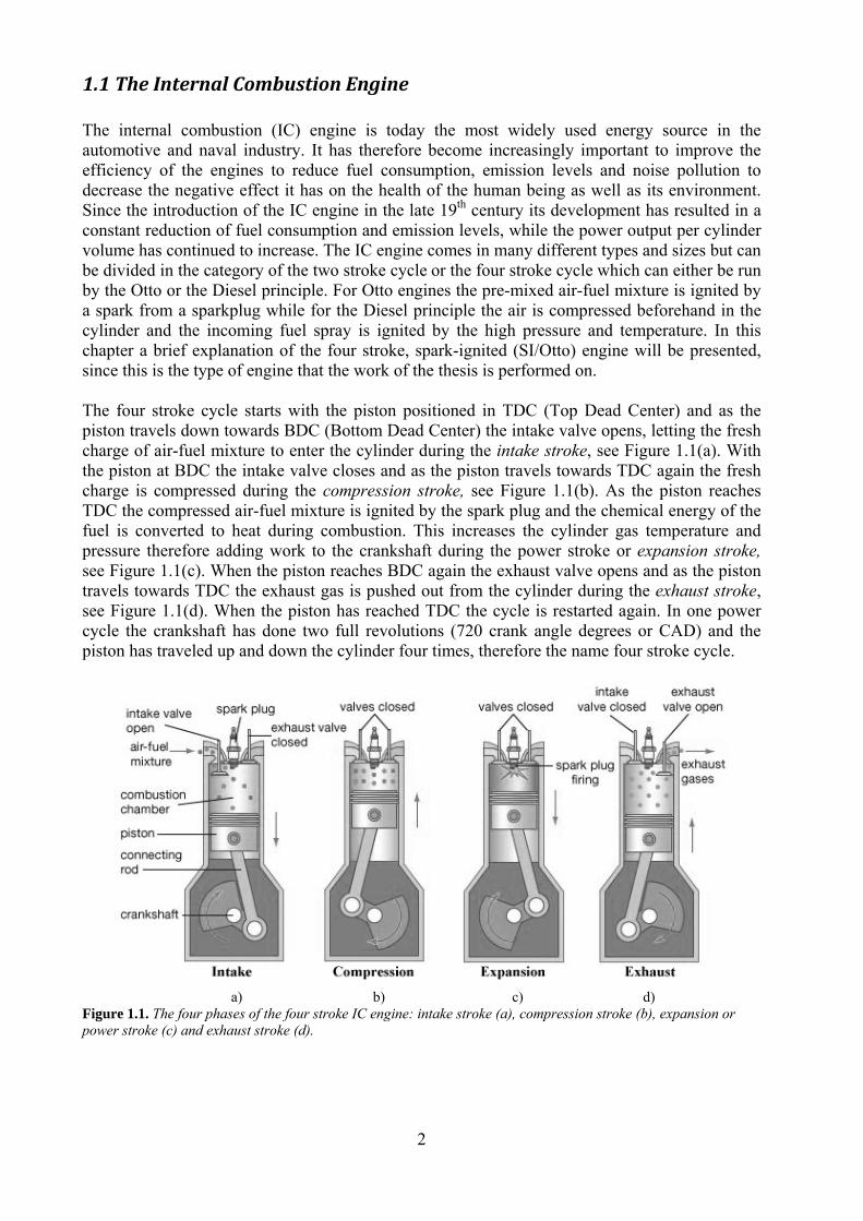
1.1 The Internal Combustion Engine  The internal combustion (IC) engine is today the most widely used energy source in the automotive and naval industry. It has therefore become increasingly important to improve the efficiency of the engines to reduce fuel consumption, emission levels and noise pollution to decrease the negative effect it has on the health of the human being as well as its environment. Since the introduction of the IC engine in the late 19th century its development has resulted in a constant reduction of fuel consumption and emission levels, while the power output per cylinder volume has continued to increase. The IC engine comes in many different types and sizes but can be divided in the category of the two stroke cycle or the four stroke cycle which can either be run by the Otto or the Diesel principle. For Otto engines the pre-mixed air-fuel mixture is ignited by a spark from a sparkplug while for the Diesel principle the air is compressed beforehand in the cylinder and the incoming fuel spray is ignited by the high pressure and temperature. In this chapter a brief explanation of the four stroke, spark-ignited (SI/Otto) engine will be presented, since this is the type of engine that the work of the thesis is performed on. The four stroke cycle starts with the piston positioned in TDC (Top Dead Center) and as the piston travels down towards BDC (Bottom Dead Center) the intake valve opens, letting the fresh charge of air-fuel mixture to enter the cylinder during the intake stroke, see Figure 1.1(a). With the piston at BDC the intake valve closes and as the piston travels towards TDC again the fresh charge is compressed during the compression stroke, see Figure 1.1(b). As the piston reaches TDC the compressed air-fuel mixture is ignited by the spark plug and the chemical energy of the fuel is converted to heat during combustion. This increases the cylinder gas temperature and pressure therefore adding work to the crankshaft during the power stroke or expansion stroke, see Figure 1.1(c). When the piston reaches BDC again the exhaust valve opens and as the piston travels towards TDC the exhaust gas is pushed out from the cylinder during the exhaust stroke, see Figure 1.1(d). When the piston has reached TDC the cycle is restarted again. In one power cycle the crankshaft has done two full revolutions (720 crank angle degrees or CAD) and the piston has traveled up and down the cylinder four times, therefore the name four stroke cycle.

a) b) c) d) Figure 1.1. The four phases of the four stroke IC engine: intake stroke (a), compression stroke (b), expansion or power stroke (c) and exhaust stroke (d).

3

The combustion process in the SI engine can be divided into four stages:

1. Spark ignition. The air-fuel mixture is ignited by the spark discharge of the sparkplug. The sparkplug releases a high energy plasma with a temperature around 60 000 K for a very short period (typically in the order of 1 ns). The spark ignition usually occurs around 20-40 crank angle degrees before TDC.

2. Early flame development. The first phase of the combustion process is the laminar flame propagation. The flame propagates in a sphere around the sparkplug and the flame front is considered smooth with a typical thickness of 0.1 mm and a velocity of around 0.5 m/s. The flame speed depends on the pressure, temperature, the air-fuel ratio and the amount of residual gases from the previous cycle. High temperature and a low air-fuel ratio results in a higher flame velocity while high pressure and residual gases results in a lower velocity.

3. Turbulent flame propagation. After a few crank angle degrees the laminar phase is transformed into a turbulent phase, caused by the turbulence created during the intake and compression stroke. The smooth laminar flame front is broken down by vortexes into a turbulent flame front with a very irregular and wrinkled shape. The flame speed now reaches velocities of 10-50 m/s. The velocity still depends on pressure, temperature, the air-fuel ratio and amount of residual gases, but the turbulence intensity is the most important factor in this phase. Increasing the engine speed leads to more generated turbulence, this in turn results in higher flame velocity. This leads to a combustion time that is unchanged (expressed in crank angle degrees) allowing for high engine speeds for the SI engine.

4. Flame extinction. Lastly the flame reaches the cylinder liner causing flame extinction because of the liner walls relatively low temperature. The combustion phase is usually completed around 30 crank angle degrees after TDC.

This is a simplified explanation of the typical combustion process where the spark ignited flame moves steadily across the combustion chamber until the charge is consumed. However two types of abnormal combustion can be identified; knock and surface ignition which will be explained in the next chapter.

1.1.1 Abnormal Combustion Phenomena  As the flame propagates across the combustion chamber the unburned mixture ahead of the flame (called the end-gas) is compressed, causing its pressure, temperature and density to increase. Some of the end-gas air-fuel mixture may then undergo chemical reactions prior to the normal combustion when the flame front reaches the end-gas. These chemical reactions may cause the end-gas to auto ignite, releasing a large part or all of their chemical energy. This causes the end-gas to burn very rapidly with flame velocities of up to 1000 m/s and it creates high-frequency pressure oscillations inside the cylinder that produce the sharp metallic noise called knock [1]. Knock is mainly caused by high pressure and temperature in the end-gas but depends also on the octane number of the fuel. Knock is common in engines with a high compression ratio ε, which leads to a high cylinder pressure and an increased risk of knock when the end-gas is compressed further by the propagating flame. The pressure waves that knock creates, lead to high mechanical load on the engine, causing damage to the material. Knock can be detected by knock sensors, for example with an accelerometer in the cylinder walls that detects high-frequency pressure oscillations. Knock can then be avoided by adjusting the spark timing automatically when knock is detected in the engine. By retarding the time of spark discharge the maximum cylinder pressure is lowered with a decreased risk of knock as result.

4

The other abnormal combustion phenomenon is surface ignition. This phenomenon is caused when the air-fuel mixture is ignited by an overheated surface in the engine, like the valves or the sparkplug. It is defined as ignition by any other source than the spark of the sparkplug. It can occur before the spark ignition (preignition) or after (postignition). Either way it means that the combustion process is no longer controlled by the ignition of the spark. When surface ignition results in knock in the end-gas it is called knocking surface ignition [1]. Knock can be considered a bigger problem than surface ignition, since surface ignition can be avoided with proper engine design. Knock on the other hand is an inherent constraint on engine performance and efficiency since it limits the maximum compression ratio that can be used with any given fuel [1].

1.1.2 Charge Motion Classifications  As explained above, the turbulence level in the cylinder is very important for the turbulent flame propagation and the efficiency of the combustion. There are many ways in which the turbulence level in the cylinder can be increased by different constructions of the intake ducts. The flow motion of the incoming fresh charge can vary dramatically depending on the design of the intake ducts, valves and combustion chamber. The structure of the flow can be divided in three main motion categories; squish, swirl and tumble, see Figure 1.2. Squish is defined as the flow created when the piston reaches TDC and the outer part of the piston crown approaches the cylinder head closely, causing a flow motion directed from the cylinder liner towards the center of the combustion chamber, see Figure 1.2(a). Swirl is the rotational flow motion around the cylinder axis and is created by the shape of the intake duct, see Figure 1.2(b). By bringing the intake flow into the cylinder with an initial momentum a swirl motion is created, usually persisting through the whole intake, compression and expansion stroke. Tumble is the rotational flow around the axis perpendicular to the cylinder axis, see Figure 1.2(c). The tumble motion is also created by the shape of the intake duct and the angle of the incoming jets of fresh charge.

a) b) c)

Figure 1.2. Charge motion classification for three typical flow structures; squish (a), swirl (b) and tumble (c). While all three of these charge motions can help to improve the turbulence level in the SI engine, the tumble motion is instead the most important. Tumble is generated during the intake stroke and intensified during the compression stroke where the large scale tumble motion keeps its angular momentum but increases its intensity because of the shrinking cylinder volume. As the piston reaches TDC and the combustion chamber becomes “flat”, the large scale tumble motion breaks up in small scale turbulence, creating a high level of turbulence intensity in the cylinder. To create a strong tumble motion it is not just important to accelerate the incoming flow, but also

5

to direct it mainly towards the area of the exhaust valve. In a traditional intake duct the incoming charge is distributed quite uniformly around the valve causing a flow that counteract itself and hinder the creation of a main tumble motion. By directing a bigger part of the flow towards one side of the valve, preferably towards the exhaust valve, a strong tumble motion can be created by this main flow jet that is not counteracted by the jets created on other sides of the valve [2]. A strong tumble motion creates high turbulence which in turn leads to a high flame velocity. This increases the efficiency of the combustion process, but the fast combustion also leads to hard engine noise. A strong tumble motion is positive for high performance and racing engines but for normal engines a compromise between engine noise levels and performance has to be made.

1.2 Purpose of the Thesis  The purpose of this thesis can be divided into two parts. The first part is related to the strategies of mesh management and CFD simulation, and the second part is related to the analysis of the results produced for the specific engine used for the simulations. Since the moving piston and valves deforms the solution domain extremely during a whole engine cycle, the computational grid will at some point become too distorted, leading to numerical errors and abortion of the calculations. A strategy to solve this was previously developed by the Internal Combustion Engine Group at Politecnico di Milano which uses a number of computational grids or meshes to cover the whole engine cycle. Each mesh is deformed for a certain interval and when the quality of the mesh becomes too low, the solution is interpolated onto a new mesh. This strategy is called the MUMMI approach (Multiple Mesh Motion and Mesh to Mesh Interpolation) and it had previously been employed on a simplified engine geometry [10] and later on a real engine geometry [12]. In the last case the calculations of the whole engine cycle intended to be simulated was not actually performed due to the fact that no real boundary conditions were used. Thus, the purpose of this thesis was to use the same strategy of how each mesh is constructed and generated as in the previous cases, but this time employed on the real and highly complex engine geometry of the F4 engine, including the use of realistic boundary and initial conditions for temperature, pressure and mass flow. The simulation was intended to cover the intake, compression and expansion stroke starting from the opening of the intake valve and ending at the completion of the combustion process. The purpose was also to study a combustion model developed by Weller [3], which is pre-implemented in the OpenFOAM code, to investigate if a realistic combustion process could be simulated for the F4 engine. The second part of the purpose of this thesis is strictly engine related. First it was of interest to make an investigation of the structure of the charge motion created during the intake and compression stroke to see if a strong tumble motion is created. As mention in Chapter 1.1.2 tumble is important for the performance of the SI engine and is mostly created by the design of the intake port and the intake valves. Furthermore, the F4 engine has a tendency to knock at full load for the engine speed that produces the maximum amount of torque, and it was of importance to try to make an investigation to why and where the knock occurs. As mentioned in Chapter 1.1.1 the knock risk depends on the temperature and pressure of the end gas and a study had to be made to see if, for example, the charge motion could create a temperature distribution in the cylinder that is not uniform, causing a higher knock risk in some parts of the cylinder. As a sub purpose it was also of interest to see if the whole process of mesh generation and simulation could be done within a reasonable amount of time to make it valid as an engineering tool.

6

1.3 Thesis Outline  After the introduction in this first chapter, Chapter 2 intends to give a brief and general overview of computational fluid dynamics and its mathematical models, followed by a description of the methods used to handle CFD calculations on a dynamic mesh with moving boundaries. Chapter 3 deals with all the necessary steps of the pre-processing, including mesh generation, boundary and initial condition assignment and setup of the OpenFOAM case for engine simulations. In Chapter 4, the results of the simulations are presented together with the different strategies used to improve the consistency with 1D calculations performed on the F4 engine. Furthermore, analyses of the calculated field values for flow velocity, temperature, turbulence etc, are also made for the final simulation. To summarize the results, Chapter 5 gives an overview of the most important conclusions that could be drawn from the work of this thesis. Lastly, in Chapter 6, a brief overview is given of suggestions for possible future work that can be done, both related to this specific engine and to engine simulations in general.

7

2. Computational Fluid Dynamics Modeling 

2.1 Mathematical Models  This chapter will give a brief overview of the models used for CFD simulation. A complete description of these models is outside the scope of this thesis and the reader is instead referred to the many references such as [3], [5], [7], and [8] for more information.

2.1.1 General Transport and Governing Equations  The main concept of CFD is the discretized solution of a set of partial differential equations commonly known as the Navier-Stokes equations. These equations are discretized in time, by solving the equations in small time steps, and in space by dividing the domain in a large number of small computational cells or control volumes (CV). The space discretized solution domain is commonly referred to as the computational grid or mesh. The method commonly used for space discretization is called the Finite Volume Method (FVM), and for a static mesh (no moving boundaries) it is based on the integral form of the conservation equation over a control volume, CV, fixed in space. But simulating the fluid dynamics in a combustion engine requires moving boundaries of the solution domain, since the structure of the flow field is very much dependent on the moving piston and valves. When the mesh has moving boundaries the integral form of the conservation equation for a tensorial property ϕ defined per unit mass in an arbitrary moving volume V bounded by a closed surface S states [4]:

· ·

where ρ is the density, u is the fluid velocity, ub is the boundary velocity and qϕ and Sϕ are the surface and volume sources/sinks of ϕ respectively. Since the volume V is no longer fixed in space, its motion is captured by the motion of its bounding surface S by the velocity ub. The first term in Equation 2.1 is the temporal derivative (or rate of change of ϕ), the second is the convection term representing the convective transport by the prescribed velocity field. The third term is a diffusion term representing the gradient transport and finally the fourth term is the source/sink term for non transport effects, which means local production and destruction of ϕ [6]. The governing equations of the general transport or conservation equation (Equation 2.1) are described below in their differential form. For more details on these equations the reader is referred to [5], [7] and [8]. • The continuity equation governs the conservation of mass, which means that the rate of

change of mass in an arbitrary control volume must be equal to the total mass flow over the control volume boundaries:

· 0

• The momentum equation governs the conservation of linear and angular momentum. According to Newton’s second law, the rate of change of momentum on a fluid particle equals the sum of forces acting on that particle:

(2.1)

(2.2)

8

∂ · g ·

• The energy equation governs the conservation of energy. This equation is based on the first law of thermodynamics that says that the rate of change of total energy of a fluid element, i.e. the sum of all energy forms (internal, kinetic, mechanical, chemical, etc.) must equal the net rate of heat and work flow over its boundaries. However, an alternative formulation of the energy equation, used in the OpenFOAM code, is the enthalpy equation:

· ·

where ρ is the density, u is the fluid flow vector, g is the body force, σ is the stress tensor, h is the enthalpy, α is the thermal diffusivity for enthalpy, αt is the turbulent thermal diffusivity, Q is the energy source term, and p is the fluid pressure. The above conservation laws are valid for any continuum, but the number of unknown quantities is larger than the number of equations in the system, making the system indeterminate. To close the system a set of constitutive relations are necessary. These are for Newtonian fluids; the internal enthalpy equation, the equation of state, Fourier’s law of heat conduction and Newton’s law of viscosity, see [5].

Figure 2.1. A polyhedral cell with the finite volume method notation

Unstructured FVM discretizes the computational space by splitting it into a finite number of convex polyhedral cells bounded by convex polygons which do not overlap and completely cover the solution domain. The temporal dimension is split into a finite number of time-steps and the equations are solved in a time-marching manner. A sample cell around the computational point P located in its centroid, a face f, its area vector sf and the neighboring computational point N are shown in Figure 2.1. Second-order FV discretization of Equation 2.1 transforms the surface integrals into sums of face integrals and approximates them to second order using the mid-point rule [4]:

∆ ·

(2.3)

(2.4)

(2.5)

9

where the subscript P represents the cell values, f the face values and superscripts n and o the “new” and “old” time level, VP is the cell volume, F = sf ·uf is the fluid flux and Fs is the mesh motion flux. The fluid flux F is usually obtained as a part of the solution algorithm and satisfies the conservation requirements [4]. For more information on how the equations in this chapter are solved, using numerical methods, the reader is referred to [6].

2.1.2 Turbulence Model  Turbulence can be found in almost all fluid flows. Turbulent flow is a flow that is irregular, random and chaotic. It can be described as a state of continuous instability in the flow, where it is still possible to separate the fluctuations from the mean flow properties. Turbulence is associated with eddies which affects the mean flow, where the range of the scales is very large, from the smallest turbulent eddies characterized by Kolmogorov microscales, to the flow features comparable with the size of the geometry [5]. The largest eddies extract their energy from the mean flow. These eddies transfer energy to smaller eddies in a cascade process. The large scale eddies have an orientation imposed by the mean flow, but the smaller eddies will not “remember” their origin and orientation and will behave isotropic, i.e. independent of direction. The scale of these eddies, referred to as Kolmogorov’s microscale, are small and dissipative forces prevails. In this regime, the kinetic energy is destroyed by viscous forces, and viscosity and dissipation affect the length scales. The cascade process, from the biggest to the smallest eddies, occurs over a wide length scale spectrum and a very fine mesh is needed to resolve the smallest Kolmogorov eddies. A very fine resolution in time is also needed, since turbulent flow is always unsteady [13]. The requirements on mesh resolution and time-step size for an exact solution of the flow, puts very high demands on computer resources, rendering it unsuitable for engineering applications. This can be solved by simulating turbulent flow using statistical methods. Using statistical or averaging methods, the local value of the variable can be separated into the mean and the fluctuation around the mean which then makes it possible to derive the equations for the mean properties themselves. The averaging methods can appear in two versions, Reynolds averaging and density-weighted Favre averaging [5]. Applying the averaging procedures to the Navier-Stokes equations will introduce an unknown term referred to as Reynolds stress tensor. This will lead to an equation system with more unknowns than available equations. This is known as the closure problem and in order to close the system, further modeling is necessary to solve the Reynolds stress tensor. A widely used method to handle the closure problem is the Boussinesq approximation, which states that the Reynold stresses are linked to mean rates of deformation by introducing a turbulent viscosity, μt [13]. The turbulent viscosity can be evaluated in many different ways but the most popular approach is to express μt as a function of the turbulent kinetic energy k and its dissipation rate ε ( / ), where Cμ is a model constant. This leads to a two-equation model referred to as the k-ε turbulence model, where k and ε are obtained by the solution of their respective transport equations. For more detailed information about the standard k-ε turbulence model and the derivation of the transport equations for k and ε, the reader is referred to [5], [7] and [13].

2.1.3 Combustion Model  The combustion model used for the simulations in this thesis is the b-Ξ Weller combustion model since it is the standard combustion model incorporated in the OpenFOAM CFD code. This model is based on the evaluation of the dimensionless variable b which describes the

10

species concentration of the combustion reactants in each computational cell. The value of variable b ranges from 0 to 1, where a value of 0 means that the combustion process is completed in the whole cell and a value of 1 means that no combustion process has taken place. The transport equation to describe the evolution of b in time and space states:

· · Ξ min  Ξ, Ξ where ρ is the density, ρu is the density in the unburnt mixture, u is the fluid flow vector, Γb is equal to / , μt is the turbulent viscosity, σh is the turbulent Prandtl coefficient, Su is the laminar flame speed. The sign ¯ indicates the average and ~ indicates the Favre average based on the density (i.e.  / ). The subscript eq signifies the equilibrium value which works as an upper limit of Ξ. Lastly, Ξ is defined as the local flame wrinkling factor, and it is defined as the ratio between the turbulent flame speed St and the laminar flame speed Su:

Ξ

There are two ways to determine Ξ. One way is by using a transport equation also for Ξ. But for some engineering purposes it may not be necessary to reproduce all the details of the flame structure or the transient response of the turbulent flame speed. Under these conditions the Ξ transport equation need not be solved at all, instead a simple analytical (or algebraic) expression for Ξ can be used in the b equation (Equation 2.6) [3]. The algebraic expression of Ξ states:

Ξ Ξ 1

where A is a free coefficient, u’ is the turbulence intensity and Su is the laminar flame speed. For a more detailed description of the b-Ξ Weller combustion model, ignition and flame initiation the reader is referred to [3] and [7].

2.2 The OpenFOAM CFD Code  There is a number of CFD software that incorporates solvers for the above mentioned equations, each in its own way. One of these is the OpenFOAM (Open Field Operation and Manipulation) CFD Toolbox which is used for the simulations of this thesis. OpenFOAM is a non-commercial open source CFD code, which means it is freely available to use and modify as the user wishes, under the restrictions of the GNU General Public License. OpenFOAM can simulate anything from complex fluid flows involving chemical reactions, combustion, turbulence and heat transfer, to solid dynamics, electromagnetics and the pricing of financial options [16]. The OpenFOAM code is basically a set of efficient C++ modules which together build a number of solvers, utilities and libraries. Solvers are executables that solve different problems, in this case computational fluid dynamic problems. Utilities are executables that perform different pre- and post-processing like data manipulation and mesh operations. Libraries can for example be a library of physical models that are accessible as a toolbox to the utilities and solvers. The C++ object oriented structure also allows easy use of already available C++ software components as for example linear and field algebra solvers, sparse-matrix solvers etc. The name OpenFOAM not only refers to the fact that it is an open source code, but also that it is open in its structure and hierarchical design making it easy for users to modify and extend the

(2.6)

(2.7)

(2.8)

11

Figure 2.2. Structure of a general OpenFOAM case including the mandatory directories, libraries and dictionaries.

existing solvers, utilities and libraries or to create their own. This is the main reason that OpenFOAM is used by the engine group at Politecnico di Milano since it offers great flexibility to implement and test new models and strategies for engine simulations. It also offers the benefit of easier troubleshooting when there are errors since the user has direct access to the source code. A short description of a typical OpenFOAM case structure will be described below.

Figure 2.2 shows the general structure of a typical OpenFOAM case. Every mesh will have its own case which means that the whole engine cycle to be simulated will contain a number of cases, for more information on mesh intervals see Chapter 3.4. The case directory (with the case name as directory name) contains three types of main directories; system, constant and all the time directories. The time directories for engine simulations will be represented by crank angle degrees (CAD) and not the actual simulation time. Each of these three main directories will be explained below. Note that in Figure 2.2 only the mandatory files to run any kind of calculation are listed, but for engine applications there are several other necessary files and not all are explained here. Some of the files are only used by other utilities and not the solver itself, and therefore they are not included in this chapter. A short description of these files can instead be found, together with the description of the corresponding utility, mainly in Chapter 2.3.3 and 3.5.

The system directory contains files or dictionaries associated with the solution procedure, these are:

controlDict – Contains settings for the simulation such as start/end time, time step, max Courant number, data writing interval and format, time step adjustments etc. fvSchemes – Contains settings for the numerical schemes used for terms such as derivates and gradients for the equations in the solvers. fvSolution – Contains settings for which equation solvers, tolerances and other algorithms that will be used for the simulation.

The constant directory contains files specifying physical and geometrical properties for the simulation, some of these are:

engineGeometry – Contains settings for the engine geometry such as bore, stroke, engine speed and minimum valve lift. It also contains information about which boundary surfaces and cell zones that should be moving during mesh motion, more on this in Chapter 3.2. thermophysicalProperties – Contains setting for the thermo physical model such as thermo physical properties, transport properties, mixture properties etc. turbulenceProperties – Contains setting for the turbulence model and its parameters. combustionProperties – Contains settings for the combustion calculations such as model parameters, fuel properties and behavior of ignition (ignition time, location, duration and strength)

12

The constant directory also contains a sub-directory called polyMesh. In this directory a full description of the case mesh is saved in a number of files such as points, cells, faces and boundary. These files contain lists of all points, faces, cells, and boundary faces of the mesh. It is also here all the cell zones and boundary patches are specified, for more information about this see Chapter 3.2. The time directories which will be named according to the time of the simulation expressed in crank angle degrees. For each case a starting time directory will be created containing all the initial conditions for the boundaries and the internal field for every field variable to be calculated. When the simulation is started the result of the calculated field values will be saved in a new folder named according to the current time. The interval for how often the calculated result will be saved can be set in the controlDict file. When the simulation of one case is finished the case directory will contain a number of time directories, each one containing the solution for the field values at the corresponding time. The post processing software (for example ParaView) then uses the data in these time directories to present the results in a graphical manner. The simulation will also produce a number of files in the case directory containing calculated averaged field values for each time step, ie; calculated mean pressure and temperature for the cylinder volume, min/max temperature or the total domain mass as function of crank angle degrees.

2.3 Methods for Dynamic Mesh Motion  When simulating internal combustion engines the mesh will never be static since there is always deformation of the mesh by either the piston or the valve motion. Using a static mesh can only give very little information of the actual flow in an engine. Therefore it is very important to be able to perform the simulation on a mesh that can be deformed by the motion of the boundary, in this case the piston and the valves. In this chapter some methods for handling dynamic mesh motion is described.

2.3.1 Automatic Mesh Motion  The motion of the boundaries is decided by the valve lift curves and the piston motion but for the internal mesh points an iterative motion solver was developed by Jasak and Tuković [4]. The automatic mesh motion solver is based on a motion equation that calculates the velocity of the mesh point. The solver is described shortly in this chapter but the reader is referred to [4] for more detailed information. The automatic mesh motion solver is based on the Laplace equation which governs the mesh motion and is solved for the point velocity field u, with constant or variable diffusivity γ, see Equation 2.9.

· 0 (2.9)

The solution provided by the Laplace operator is always bounded also when the diffusivity is not uniform within the computational domain [10]. The position of the mesh points are then calculated with Equation 2.10.

∆ (2.10)

13

Figure 2.3. Decomposition of a polyhedral cell into tetrahedral cells.

(2.11)

Where xold and xnew are the point positions before and after mesh motion, and Δt is the time step. Solving the Laplace equation for the motion velocity instead of the point positions is preferred since the velocity changes slower and a better initial guess is available and it reduces round-off errors [4].

To preserve the mesh validity during mesh motion and to avoid degenerate cells, the motion Equation 2.9 is discretized by a second order tetrahedral finite element method. This discretization produces a sparse and symmetric positive definite matrix, which allows the use of an iterative solver called Algebraic Multigrid (AMG). This discretization requires the polyhedral cells to be consistently decomposed into tetrahedral cells. This is done on the fly by the solver by introducing a point in the cell center and split the faces into triangles, as can be seen in Figure 2.3. Consistency in tetrahedral connectivity is obtained by using identical face decomposition for cells that share an internal face. The automatic mesh motion strategy will preserve mesh quality and validity for an arbitrary interval, but eventually the mesh will become too compressed or stretched which will impact the quality of the solution. A way to check this is described in the following chapter.

2.3.2 Mesh Quality Indexes  With dynamic mesh motion it is important to be able to control the quality and validity of the mesh because of the mesh deformation that takes place. Mesh distortion and invalidity is responsible for increasing calculation time and numerical errors. The OpenFOAM code uses several indexes to control the quality and validity of the mesh. These are aspect ratio, skewness and non orthogonality and they are explained in this chapter. The aspect ratio mesh quality index is defined for tetrahedral cells as the ratio between the maximum edge length l and the minimum cell height h, see Equation 2.11 and Figure 2.4(a).

   max min 

For hexahedral cells aspect ratio defined in a similarly way. Aspect ratio is an index describing the quality of the cell volume and a very high value can lead to inverted cells.

a) b) c) Figure 2.4. Definitions of mesh quality indexes. Aspect ratio (a), non orthogonality (b) and skewness (c).

14

Mesh non orthogonality is defined as the angle α between the face area vector S and the vector d connecting the cell centers (P and Q) of the cells that share the same face (with face center f), see Figure 2.4(b). Non orthogonality affects the discretization accuracy of the diffusion term in transport equations [5]. Non orthogonality is common in meshes with complex geometries that require tetrahedral cells. If the value of α is larger than 70º the non orthogonality is considered severe, leading to increased computational time and quality of the solution [5]. A value of α greater than 90º results in an invalid mesh since the cells will be distorted. Mesh skewness for a face is defined as Equation 2.12.

 

Where m is the distance between the face centre f and the intersection fi, which is the intersection of the face area between two cells and the vector d. Vector d is connecting the cell centers (P and Q) of the cells that share the same face and has the face area vector S, see Figure 2.4(c). Mesh skewness reduces the accuracy of face integrals [5] since the interpolated face value does not lie in the center of the face f, but instead lies in the intersection fi. High skewness is expected in meshes with complex geometries and tetrahedral cells. Skewness is considered severe when it is higher than 4 but values lower than 10 can still be acceptable [10].

2.3.3 Quadratic Diffusivity  A way to improve the quality of the mesh and to reduce the local deformation of cells close to the moving boundaries is by increasing the diffusivity γ in Equation 2.9. This is done by changing the diffusivity formulation in the dynamicMeshDict dictionary in the constant folder of the OpenFOAM case. The user also chooses which boundary surfaces that the diffusivity formulation will be used on, as a function of the cell center distance l to the nearest selected boundary. Mostly a linear diffusivity ( ) was used during the work of the thesis. But when there was a rapid decrease in mesh quality, the quadratic formulation ( ) was also tested as a way to improve the local deformation of the cells close to the boundaries. An example of mesh deformation close to the valve using linear and quadratic diffusivity is shown in Figure 2.5.

a) b)

Figure 2.5. Mesh motion using linear (a) and quadratic (b) diffusivity on the boundary surface of the underside of the valve plate. Images are taken after valve has been moved 18 CAD from the original starting position of the mesh.

(2.12)

15

Figure 2.6. Definition of closest (cyan) and neighboring cells (green) in the source mesh for a cell in the target mesh (red). ci cell center of cell i in the source mesh, x cell center of the target mesh.

(2.13)

It is visible that the cells close to the valve bottom are very compressed (see circle in Figure 2.5(a)) when using linear diffusivity, while the cell of the same area are well preserved when using quadratic diffusivity as in Figure 2.5(b). Note that in this case the cells close to the piston are instead very compressed when using quadratic diffusivity for the valve boundary surface, this because the valve is very close to the piston. The mesh quality as a whole is not improved, but Figure 2.5 serves only as an example of how the cells can be locally improved close to the chosen boundary. There are also other formulations of diffusivity but quadratic diffusivity was chosen since it offers the best compromise between mesh quality and computational time, for more information regarding diffusivity the reader is referred to [4].

2.3.4 Mesh Management  When using the mesh motion technique described in Chapter 2.3.1 and moving the boundaries, the mesh will eventually become too distorted with numerical errors as result. By looking at the mesh quality indexes it is possible to see when this occurs and decide the interval for which the mesh is valid. Since one mesh cannot cover a whole engine cycle with moving valves and piston the MUMMI (Multiple Mesh Motion and Mesh to Mesh Interpolation) approach was developed at the Internal Combustion Engine department at Politecnico di Milano [10]. This strategy uses a number of meshes to cover the whole engine cycle to be simulated. The solution for the field quantities (pressure, temperature, enthalpy etc.) of the initial (source) mesh is consistently interpolated onto a new (target) mesh when the initial mesh has become too distorted because of the boundary motion. This is repeated until the whole simulation cycle is covered by a number of meshes, and the solution at the end of one mesh interval is interpolated onto the start of the next mesh interval. The mesh to mesh interpolation technique which uses a second order, inverse distance weighting method [10], is described below. For each cell center on the target mesh, the closest cell center of the source mesh is located, see Figure 2.6. The field values for each cell center of the target mesh (x) are then calculated as a function of the field values of the corresponding cell center of the source mesh and its closest neighboring cells (ci), see Equation 2.13.

1∑   ,

1| |

Where ui are the field values of the source mesh and x and ci are the cell centers as described above and in Figure 2.6. If the distance between the target (red) and the closest source cell center (cyan) is less than 1 % of the shortest edge size in the mesh, no interpolation is performed. Instead the field values of the target cell are set equal to the values of the closest source cell. The consistency and accuracy of the interpolation technique were tested thoroughly in [10] where a set of meshes was used to calculate the flow field of a simplified engine geometry with a centrally located valve. After the solution of each mesh had been mapped onto a new mesh the consistency of the solution was investigated in terms of; conservation of

16

total domain mass, velocity profiles along the valve and mass flow at the valve exit plane. Each of these three parameters showed very small or negligible differences between the source and the target mesh. Relative differences of the total domain mass were for example reported as less than 0.002 % [10].

2.3.5 Valve Closure Problem  One problem with the moving mesh strategy is the valve closure. As the valve moves closer and closer to the cylinder head it will cause the cells between the top of the valve and the cylinder head to become more and more compressed. Eventually they will have very low quality or even be inverted or have zero volume which results in numerical errors and abortion of the calculation. An approach to simulate the contact between the valve and the cylinder head was developed in [9] and is called attach-detach boundary. When the valve lift is lower than a pre-set arbitrary value (usually ~0.1 mm) the valve is considered closed. At that time a set of internal faces at the valve curtain (black faces in Figure 2.7) are converted into a double set of boundary faces.

a) b)

Figure 2.7. Valve closure simulated using the attach-detach boundary approach. In (a) the valve is considered open and in (b) a set of internal faces are converted to wall boundaries (black) to close the valve. These two new set of boundary faces will separate the cylinder volume from the duct volume by acting as a wall boundary (one set of faces for the cylinder volume and one set for the duct volume). In this way the valve is simulated as closed without changing the geometry of the valve or the cylinder head, and there is no need to modify the solver or the mesh. This change in mesh topology is easy to execute with the OpenFOAM code and can be user triggered at a specific time in the simulation. There will be a small change in the valve opening and closure time but if the value of minimum valve lift is small the difference will be negligible.  

17

3. Pre Processing 

3.1 The MV Agusta F4 Engine  The engine geometry used for the simulations carried out in this thesis was provided by MV Agusta. The CAD model is from the engine called F4 that is used for all the F4 motorcycle models made by MV Agusta. The basic F4 engine (see Figure 3.1) has four cylinders with a total displacement of 1000 cc with four valves per cylinder. It has port injection and a centrally located spark plug in the pent roof type cylinder head. See Table 3.1 for detailed engine data.

Table 3.1. Engine data. Bore 76 [mm]Stroke 55 [mm]Connecting rod length 107.3 [mm]Crank radius 27.5 [mm]Clearance at TDC 0.8398 [mm]Max. exhaust valve lift 7.69 [mm]Max. intake valve lift 8.75 [mm]EVO / EVC 126 / 404 [CAD]IVO / IVC 312 / 622 [CAD]Compression ratio 13:1 [-]Power 128 kW at 13000 rpmTorque 111 Nm at 8000 rpmMax. engine speed 13000 rpm

Figure 3.1. The MV Agusta F4 engine. In the original CAD model of the engine fluid domain geometry, see Figure 3.2, the two intake valves and the two exhaust valves are visible as well as the intake duct (left) and exhaust duct (right). Both exhaust valves and intake valves are canted from the cylinder axis and from each other, more referred to as radial valves. As can be seen the two ducts from the exhaust valves and the two ducts from the intake valves are merged into one single intake port and one single exhaust port. Also note that the geometry is perfectly axially symmetrical and therefore only half of the geometry was used for the simulation.

Figure 3.2. Original CAD geometry of the fluid domain and the valves of the F4 engine.

18

(3.1)

Since several meshes need to be created during the engine cycle as explained in Chapter 2.3.4, it is important to know the exact location of valves and piston at these points, expressed in crank angle degrees (CAD). Lift profiles for the valves were provided for every second CAD from the 1D simulations made in Gasdyn. The piston position was instead calculated based on the known values of the clearance between piston and cylinder head at TDC, the connecting rod length and the stroke length, see Figure 3.3.

Figure 3.3. Scheme of engine geometry.

To calculate the distance between the cylinder head and piston at any given time Equation 3.1 was used.

· 1 cos · 1 · sin ,    2

Where x is the distance between piston and cylinder head, c is the clearance between cylinder head and piston at TDC, r is the crank radius, S is the stroke length, l is the connecting rod length, and φ is the crank angle from TDC in radians. The calculated piston position and valve lift profiles for the whole engine cycle of 720 CAD is shown in Figure 3.4.

Figure 3.4. Valve lift profiles and clearance between piston and cylinder head as a function of crank angle degrees.

0

10

20

30

40

50

60

0

1

2

3

4

5

6

7

8

9

10

0 90 180 270 360 450 540 630 720

Distance be

tween piston

 and

 cylinde

r he

ad [m

m]

Valve lift [m

m]

Crank Angle [deg]

Intake ValveExhaust ValvePiston

19

This data was then used to define the valve and piston position when a new mesh had to be made. When running the simulation in OpenFOAM, the valve position and velocities are calculated based on the valve lift profile provided in Figure 3.4 and it is imported as a list in the constant directory. The piston position and velocity is instead calculated on the fly by the OpenFOAM code while the simulation is running, using the same type of equation as Equation 3.1. It is necessary to define the values of connecting rod length and stroke length in the engineGeometry dictionary found also in the constant directory. More about the OpenFOAM case structure can be found in Chapter 2.2.

3.2 Mesh Generation Process 

3.2.1 Mesh Generation with Gambit  Because of the quite complex geometry of the cylinder head and piston crown of the F4 engine, especially considering the valve and valve pocket interaction, an advanced mesh generation software was needed that could handle meshes of all types of cell shapes. It is also necessary that the software can handle several different cell zones, each containing different cell shapes, within the same mesh. Since the MUMMI approach is used in this work there was also a demand of being able to make new meshes in an easy and fast way based on an initial first mesh. The software that was chosen and fulfilled these above mentioned criteria was Gambit v.2.3.16 (Fluent.Inc.). Gambit can import most of the common CAD geometry file formats and they are converted to consist of vertices, edges, faces and volumes. Gambit is able to automatically or manually generate meshes based on triangles/rectangles (2D) or hexahedral, tetrahedral, wedge and prism elements (3D). Note that every volume can only contain one type of cell shape, and therefore it is necessary to divide the geometry into different sub-volumes if the whole engine geometry should consist of different cell shapes [15]. The most important feature of Gambit, and the main reason to use this software, was the Journal function which basically creates a script file with all the commands received by the user input. This allows for very fast automatic creation of new meshes once an initial mesh has been made manually. More about the Journal function can be found in Chapter 3.3.

3.2.2 Geometry Cleanup  The first thing that had to be done after importing the original CAD model of the engine was to clean it from bad geometry, which means removing holes, sharp angles, unnecessary vertices, short edges, and small faces. All these defects will affect the final number of cells in the mesh since for example, each cell side can only exist in one face, and a cell side cannot cross between two edges. Many short edges and small faces will lead to a dramatically increased number of cells in the mesh, and therefore a lot of time was spent to clean the geometry. This kind of bad geometry is visible in Figure 3.2, especially around the exit of the exhaust port and in the connections between the intake/exhaust ducts and the cylinder head. In some areas it was possible to simply merge the small edges and faces together without losing the original geometry, but in other parts this resulted in an error where Gambit could not re-create the original geometry after merging the edges/faces. Cleaning these problematic areas of the engine geometry was very time consuming since most of the time the geometry had to be re-created manually by hand while paying high attention to not lose too much information of the original engine geometry. One of these problematic areas was in the connection between the ports and

20

the cylinder head, as can be seen in Figure 3.5, where there are a lot of thin faces around these connections. Examples of the geometry before and after the cleanup process can be seen in Figure 3.5 and 3.6.

a) b)

Figure 3.5. Connections between ports and cylinder Figure 3.6. Exhaust port before (a) and after (b) head before (top) and after (bottom) cleanup. cleanup

3.2.3 Geometry Decomposition  As mentioned previously the engine geometry is perfectly symmetrical around the cylinder axis and therefore the geometry could be cut in half, only containing one exhaust valve/port and one intake valve/port, to save memory and CPU load during calculations. Further on a decomposition of the geometry had to be made to be able to use a fully unstructured mesh, since each volume in Gambit can only contain one type of cell shape. The reason to use different cell types throughout the whole engine geometry is first because of the mesh motion strategy that is used, explained below. Secondly it is then possible to use tetrahedral elements where the geometry is complex and to use hexahedral cells around the valves to better follow the flow and avoid non orthogonality between cells. The mesh motion strategy that is used for this work was previously developed by the combustion engine group at Politecnico di Milano and was tested on a simplified engine geometry [10] and later validated on a more complex Piaggio engine geometry [12]. It was possible to adapt the same strategy of engine geometry decomposition also on the F4 engine used in this thesis. The remainder of this chapter is dedicated to an explanation of the geometry decomposition and mesh motion strategy. The engine geometry is divided into four different cell zones, each cell zone containing one or more sub-volumes with the same motion properties and cell type. The four cell zones are (see also Figure 3.7):

• Deforming zone - Consists of the cylinder volume. This zone will be deformed by the valve and piston motion.

• Layering zone - Located above the valve, between valve curtain and valve stem. This zone is deformed by the valve motion.

• Rigid motion zone - Located between the layering zone and the valve. This zone keeps its geometrical shape throughout the whole engine cycle, but follows the valve motion.

• Static zone - Consists of all volumes that are unaffected by boundary motion, and that keep their geometry and position during the whole engine cycle. This zone includes all remaining volumes in the intake and exhaust ports.

21

Figure 3.7. Decomposition of engine geometry into cell zones. Deforming zone (green), layering zone (yellow), rigid motion zone (purple) and static zone (red). Note that pictures are taken with different valve lift, and therefore the layering zone is thicker on the right hand side. The deforming zone and layering zone are the zones that will be affected by the boundary motion of the piston and valves, all other zones will keep their original mesh structure during the whole engine cycle. Therefore it is the deformation of these two zones that determines when new meshes have to be made. The function of the rigid motion zone is to capture the concave valve shape without affecting the layering zone. In this way it is easier to make new meshes at different valve lifts by simply adding or removing layers of cells in the layering zone. It also helps to preserve the mesh quality in the area of the valve exit. With these four zones it becomes easier to control the mesh quality during piston and valve motion. Whenever the mesh quality in the deforming zone or layering zone becomes too low (see Chapter 2.3.2 on how this is controlled), a new mesh is made by adding or removing layers in the layering zone and re-meshing the deforming zone with more or fewer cells (depending on if the cells are compressed or stretched during piston motion). In the cell zones of complex geometry (deforming zone and static zone) tetrahedral cells are used to capture this complex geometry in an easier way. In the cell zone with a more simply geometry (layering zone and rigid motion zone) hexahedral cells are used to follow the flow field and to ensure a higher mesh quality. The two sub-volumes (part of static zone) directly above the layering zone was created to have a transition of hexahedral cells where the flow reaches the valve region to preserve mesh quality, since the rest of the port had to be meshed with tetrahedral cells because of the complex geometry. As can be seen in Figure 3.7, layering zone and rigid motion zone each consists of two sub-volumes (for each valve) and the static zone consists of three sub-volumes (for each port). This is because Gambit cannot generate mesh of hexahedral elements in a closed ring volume and therefore they had to be split. To sum up, the original engine geometry was first divided in half, and then decomposed into 15 different sub-volumes, each part of one of the cell zones: deforming zone, layering zone, rigid motion zone and static zone.

3.2.4 Initial Mesh Generation  As mentioned previously the reason to use an unstructured mesh with different cell types throughout the whole engine is mainly because of the complex geometry. With this strategy it is then possible to use tetrahedral cells in parts with complex geometry and use hexahedral cells in areas where it is important with a higher mesh quality, by decomposing the geometry in less complex sub-volumes. The advantage of using an unstructured mesh is that it allows for easier and faster mesh generation since it can be a big challenge to create a mesh of hexahedral cells in

22

complex geometries. The disadvantage is instead that a mesh with tetrahedral cells will contain more cells then a mesh with hexahedral cells with the same cell size. Other disadvantages of using tetrahedral cells is that it increases the risk for numerical diffusion, the solvers for the algebraic equation systems are slower, and there is a demand of a higher memory capacity (because of higher mesh resolution) [12]. To investigate these simulations validity as an engineering tool it was desirable to keep the cost of the calculations as low as possible, in terms of memory usage and CPU load. It was necessary to make the mesh as coarse as possible without losing information about the geometry or risking to not capturing the correct in-cylinder motion and turbulence during calculations. Therefore when creating the first template mesh (which all other meshes during the engine cycle is based on) focus was put on keeping the cell numbers down as much as possible while preserving the original geometry. The first cell zone to be meshed was the layering zone. The number of cells in this zone more or less decides the total cell count in the whole mesh. Creating a very fine mesh in this zone will increase the number of cells needed in the zones connected to it, which means all other cell zones, thus increasing the total cell count dramatically. But by creating a too coarse mesh in the layering zone there can be a risk that the calculations will not capture the correct flow around the valves at opening and closure. The cell size in this zone is therefore a compromise between the total cell count in the whole mesh and the quality of the calculated result. The layering zone was meshed with hexahedral cells and the grid lines of these volumes were adapted to the expected streamlines of the flow around the valve to lower the influence of mesh non-orthogonality. Another important advantage of using hexahedral cells in layers above the valve, as can be seen in Figure 3.8, is that the deformation of this layering zone during valve motion can easily be predicted and re-meshing for a new simulation interval becomes easier. When the layering zone has become too stretched or compressed because of valve motion this zone is easily re-meshed by adding or removing layers of cells and thus keeping the same cell size. The average cell height and width in this zone was set to 0.5 mm while the length at the valve exit was set to 2 mm to keep the cell count down, see Figure 3.8. Note that at very small valve lifts (< 3 mm) the cell height had to be changed to between 0.15-0.5 mm, depending on the lift, to ensure that there were enough layers in the zone. When meshing volumes with hexahedral elements it was necessary to first pre-mesh the edges and faces of the volume by hand before creating the volume mesh, and this increased the time for mesh generation dramatically.

Figure 3.8. Static zone (red), rigid motion zone (purple) and layering zone (yellow) after mesh generation. Section is made through the middle of the valve. Definition of cell measures on the right.

23

The rigid motion zone was also meshed with hexahedral cells, trying to adapt the gridlines to the expected flow streamlines on top of the valve, as can be seen in Figure 3.8. The average cell size close to the layering zone is 1 mm while close to the valve they are 2 mm, to keep the number of cells down. The connection volumes (red in Figure 3.8) above the layering zone that are part of the static zone were also meshed with hexahedral cells. As explained above, these volumes acts as a transition between the hexahedral cells in the layering zone and the tetrahedral in the port since the port geometry is too complex to mesh with hexahedral. They were meshed with an average cell size of 0.5 mm close to the layering zone and the rest of the volume ranging from 1-2 mm in cell size. When these volumes had been meshed, it was then easy to generate a tetrahedral mesh in the intake port with an average cell size of 2 mm close to the walls and internal cell size of 3 mm. Note that in at the internal faces between a volume of hexahedral cells and tetrahedral cells, gambit generates pyramid shaped cells as a connection between the two cell types. The cylinder volume or the deforming zone needed some manual meshing of the faces before the volume mesh of tetrahedral cells could be generated. Since the geometry is quite complex around the valves and the valve pockets (see Figure 3.9) the faces of these areas had to be meshed before with a smaller cell size to correctly capture the geometry. Special attention had to be paid around the connection between the layering zone and the deforming zone to avoid distorted cells with low mesh quality index. The faces in these areas were meshed with a triangular grid with a cell size of 0.5-1 mm while the rest of the faces were meshed with a constant cell size of 1 mm. The volume mesh was then generated with tetrahedral cells with a cell size of 2 mm. This means that the mesh is refined around all the boundaries of the deforming zone, to capture the wall flow more correctly, while the internal mesh is coarser to keep the cell count down.

Figure 3.9. Deforming zone after mesh generation. Cylinder head faces on the left and piston crown faces on the right. After the meshing had been finished the decision to not include the exhaust stroke was taken because of problems with the boundary conditions in a previous work [12]. In that work wrong imposed boundary conditions at the exhaust port led to numerical errors and abortion of the calculation and therefore it was decided to only include the intake stroke, since there was a risk that the same problem could occur also in the present work. Therefore the static zone, layering zone and rigid motion zone of the exhaust port could be removed since the exhaust valve would be kept closed for the whole simulation. With only the cylinder and the intake duct left the total cell count for the first template mesh (that all the other meshes will be based on) at TDC reached 72 628 cells. This can be considered as a very coarse mesh, while still keeping an acceptable mesh resolution around the valve.

24

3.2.5 Boundary and Continuum Type Specification  To define the different cell zones and boundary faces of the engine model for the mesh motion strategy, Gambits boundary and continuum type specification was used. These definitions describe the physical property of the models different volumes and faces and Gambit takes these definitions along with the mesh when it is exported. The different boundary types that can be assigned to the faces are for example: wall, interior, pressure inlet, velocity inlet etc. and continuum types for the volumes are fluid and solid. Note that when importing the mesh, OpenFOAM does not take these boundary and continuum type definitions into account, it only acts as a way to group faces together into boundary patches and volumes into cell zones. It is then necessary to define all the boundary patches and cell zones with the correct physical properties when setting up the calculations in OpenFOAM. Each boundary patch or cell zone consists of faces or volumes that have the same physical properties or the same motion, deformation or static conditions. The definition of the boundary patches and cell zones followed the same strategy developed in [10] and later repeated in [12], to correctly take into account the motion and physical properties of the different faces and volumes according to the mesh motion strategy explained in Chapter 2.3. Another reason for specifying different boundary patches is so that different boundary values can be set to these patches. For example two patches might have the same motion properties (as is the case of cylinder head and intake duct faces which remains static during mesh motion) but the boundary values for the temperature can differ by several hundred Kelvin between the cylinder head and the intake port, and therefore it is necessary to separate them. The same goes for several other patches of the engine geometry. To define the four cell zones described in Chapter 3.2.3, the 8 sub-volumes of the engine model were defined in four different continuum zones with the same names as the cell zones: deforming zone, layering zone, rigid motion zone and static zone. This is done to group the sub-volumes of the same cell zone together and define it with a uniform nomenclature that is later used in OpenFOAM to specify that cell zone in the code. All the cell zones were defined as continuum type fluid but note that the type does not matter since OpenFOAM does not take this into account. As mentioned before this definition is only made to group the volumes together into zones and give these zones a name when exporting the mesh. The same was done with all the external faces of the engine geometry. As explained above all faces with the same physical properties were grouped together into different boundary patches. Each boundary patch has a unique motion condition or physical property and they were defined as follows, see also Figure 3.10 and 3.11:

• Moving piston – All external faces of the piston crown surface. This patch will move with piston velocity while keeping its original structure during mesh motion.

• Liner – All external faces around the cylinder liner. This patch will be deformed during mesh motion.

• Cylinder head – All external faces in the cylinder head. This patch will be static and keep its original structure during mesh motion.

• Inlet duct – All external faces of the inlet duct. This patch will be static and keep its original structure during mesh motion.

• Pressure inlet – The face at the intake port where the mass flow enters or exits. The time-varying boundary conditions for mass flow and temperature is set to this patch.

• Symmetry plane – The two faces created at the cylinder and intake port when splitting the geometry in half. This patch will be deformed during mesh motion.

25

Figure 3.11. Boundary patch definition. Valve stem (blue), moving valve (yellow), moving valve side (green), moving valve bottom (orange) and detach faces (red). Note that only one detach face is displayed for sake of visibility.

• Valve stem – All faces of the valve stem, including faces attached to the layering zone but not below it. This patch will be deformed during mesh motion because of valve movement.

• Moving valve - All faces on top of the valve. This patch will keep its original structure but will move with valve velocity.

• Moving valve bottom - All faces on the underside of the valve plate. This patch will keep its original structure but will move with valve velocity.

• Moving valve side - All faces on the side of the valve plate. This patch will keep its original structure but will move with valve velocity.

• Detach faces – The two faces connecting the layering zone to the deforming zone. This patch will initially have no other properties then the other internal faces that are not defined in one of these boundary patches. But they are marked and defined with a name so that when the valve is reaching closure they will be defined as a wall patch between the duct and the cylinder, to detach the two volumes from each other. See Chapter 2.3.5 for explanation of how the valve closure problem is solved.

Figure 3.10. Boundary patch definition. Moving piston (cyan), liner (orange), cylinder head (green), intake duct (red), pressure inlet (blue) and symmetry plane (purple).

All other faces that are not included in these boundary patch definitions are the internal faces between all the different sub-volumes. By not specifying these internal faces in the boundary specification of Gambit they will be set to internal faces by default when importing the mesh to OpenFOAM. When geometry decomposition, mesh generation, boundary and continuum type specification was finished the mesh could be exported into a single mesh file with the extension .msh. The file contains all the geometrical information about the models vertexes, faces and cells of the mesh as well as the boundary and continuum specification. The file is written in ASCII format and can be read by a standard utility in OpenFOAM called fluentMeshToFoam. See Chapter 3.5.1 for a more detailed explanation of this mesh conversion utility.

26

3.3 Automatic Mesh Generation  As mentioned in Chapter 3.2.1, one of the reasons for choosing Gambit for mesh generation was its Journal function. This function makes it possible to generate new meshes at arbitrary piston and valve positions in a simple and fast way, based on the primary template mesh that had to be made manually. The Journal function works like a script that saves all the commands that the user executes, and these commands are saved to a text file or journal file that later can be run in Gambit to re-create all the commands and operation that were done to the geometry. The journal file was created by using the initial mesh that was created manually according to Chapter 3.2.4 as a template mesh. This template mesh was created with piston at TDC and valve at 0.25 mm lift which is considered as a closed valve. With this template mesh as starting point all the commands necessary to move the piston and the valve and then recreating the mesh at these new positions was carried out manually and saved to the journal file. Without going into too much detail of all the commands that was saved to this file the procedure for creating the journal file is described below. First all the faces connecting the moving boundaries to the fixed boundaries had to be removed, which means the liner faces and the detach faces at the valve curtain. Then all the moving boundaries (piston faces and valve faces) were translated to an arbitrary (but realistic) piston position and valve lift. After that, all the vertexes, edges, faces and volumes were re-created using the same names as the deleted ones. When the geometry had been re-created the mesh of the layering zone and the deforming zone could be generated again according to the same procedure as described in Chapter 3.2.4. All the commands that are necessary for the above described operations were then saved to a journal file. It is possible to edit this journal file by hand, to change the necessary parameters when creating a new mesh with a new piston position and valve lift. Parameters that are always changed when creating a new mesh are obviously the translation of piston faces and valve faces, but in some cases also the cell size had to be modified in some parts. For example, with a very small valve lift the height of the cells in the layering zone had to be changed or when the piston is close to TDC the mesh of the liner faces had to be altered. This is then easily realized by just editing the journal file instead to be forced to create a new mesh again by hand. The procedure to create a new mesh with the journal function is dramatically reduced compared to being forced to create them manually every time. After the journal file is finished, all that has to be done is to edit the journal file according to the values of Figure 3.4 for piston position and valve lift, and then run this journal file on the template mesh file in Gambit. In total it takes around 10 minutes for a new mesh to be generated instead of taking several hours if one was forced to create the mesh manually.

3.4 Mesh Intervals  With the MUMMI approach, explained in Chapter 2.3.4, a new mesh is created as soon as the mesh quality indexes are below certain levels, and the solution of the old mesh is mapped on to the new mesh. But at some points the calculations could abort because of numerical errors even if the mesh quality indexes did not show any drastic changes. What the cause is of this problem is not always easy to predict but this problem occurred especially at the beginning of the simulation when the flow field had to be established from an initial starting flow field that was zero. Another part when this problem occurred was close to TDC when the valve and piston interaction causes the intake valve to be “surrounded” by the valve pocket. Even if the mesh quality indexes could show a very small degeneration it still led to numerical errors and abortion

27

of the calculation. By creating a new mesh at these points (or a few CAD before the error occurs) it was possible to solve the problem. The conclusion is that generally it is safe to look at the mesh quality indexes to see when it is necessary to make a new mesh to continue the calculation on. But at some points there can be problems with the mesh even if the mesh quality indexes do not show this directly, and a new mesh has to be made at an earlier point. Note that all the meshes needed to cover the whole engine cycle to be simulated, were not created in advance. Instead the calculations were started immediately on the first mesh and whenever it was necessary with a new mesh, it was created at that point, and the calculations continued. But for the sake of clarity all the mesh intervals needed for the whole simulation is shown already in Figure 3.12.

Figure 3.12. Number of cells and crank angle validity for every mesh used in the simulation compared with valve lift and piston position curves. Numbers in bars indicates the mesh number. The first mesh was created at 333 CAD when the intake valve is considered to still be closed (< 0.25 mm valve lift). In this way the whole intake stroke will be simulated while ignoring anything that happens before since the exhaust port was removed. The downside to this is that the valve overlap period is instead not correctly accounted for with some error in the volumetric efficiency as a result, as will be discussed in Chapter 4.1. The last mesh is valid until 780 CAD since at this point combustion should be completed. The whole engine cycle interval to be simulated covers 333-780 CAD with a total of 18 meshes as can be seen in Figure 3.12. It is clearly visible that the number of cells in the mesh is related to the piston position and the increasing volume of the combustion chamber when the piston distance to the cylinder head increases. The interval for which the mesh is valid is instead mostly related to the valve lift profile as also can be seen in Figure 3.12, especially around valve opening and valve closure there was a need for shorter mesh intervals to keep its quality. This is because the valve velocity is at its highest here and every crank angle degree the valve moves a longer distance then it does around maximum valve lift. The result is that the cells are deformed more for every crank angle degree around valve opening and closure. But even with the valve closed, there is a need to shorten the mesh intervals when the piston reaches TDC (at ~720 CAD) even though not as dramatic as when there is the valve opening (at ~360 CAD). This is mainly because the liner faces becomes very thin at this point with more distortion of the cells as a result.

0

30

60

90

120

150

180

210

240

270

0

1

2

3

4

5

6

7

8

9

330 360 390 420 450 480 510 540 570 600 630 660 690 720 750 780

Num

ber o

f cells [k

Cells]

Valve

 lift [m

m] a

nd  piston po

sition

 from

 cylinde

r he

ad [cm]

Crank Angle [deg]

Mesh Size [kCells]

Intake Valve Lift [mm]

Piston Position [cm]

15

3

4

6

7

89 10

1112

13

14

1516

17182

28

The mesh quality index that is used to decide if it is necessary with a new mesh is non-orthogonality, skewness and aspect ratio as described in Chapter 2.3.2. The limit for non-orthogonality in OpenFOAM is set to 70 and faces with an index above that are considered severely non-orthogonal. A non-orthogonality index above 90 results a mesh that is not valid anymore. The limit for skewness is set to 4 and faces with an index above that are considered severely skewed. Note that it is possible to run the calculation with a higher value than 4 but it is not recommended since it can increase the numerical errors. The limit for aspect ratio is set to 1000 and value higher than that results in an invalid mesh. For all the 18 meshes the aspect ratio never exceeded a value of 60 and therefore it was only necessary to look at non-orthogonality and skewness, see Figure 3.13.

Figure 3.13. Number of severely non orthogonal faces and maximum skewness for all the mesh intervals.

As can be seen the limiting factor for all the meshes is the non-orthogonality except for mesh number 3 where it is the skewness that is the limiting factor. The number of severely non orthogonal faces increases quite dramatically in the end of almost every mesh interval and this is the reason why a new mesh is needed. There are some exceptions to this and they are discussed below. In the first mesh interval there is a dip of non orthogonal faces before it rises again. This is because in the first mesh, when the valve lift is very small, it was necessary to create very thin layers in the layering zone to have at least more than 1 layer in total. These very thin layers created a lot of non orthogonal faces around the valve curtain, but as the valve lift increases the layers were stretched and became thicker with an improvement in the non orthogonality as a result. As the valve lift continued to increase these layers became too stretched and the number of severely non orthogonal faces increased again as is visible in Figure 3.13. The second mesh was also an exception to the general rule, where there is neither a high skewness index nor a high number of non orthogonal faces, but the calculation still aborted due

MESH 1

MESH 2

MESH 3

MESH 4

MESH 5

MESH 6

MESH 7

MESH 8

MESH 9

MESH 10

MESH 11

MESH 12

MESH 13

MESH 14

MESH 15

MESH 16

MESH 17

MESH 18

‐1,0

‐0,5

0,0

0,5

1,0

1,5

2,0

2,5

3,0

3,5

0

100

200

300

400

500

600

700

800

900

330 360 390 420 450 480 510 540 570 600 630 660 690 720 750 780

Maxim

um skewne

ss

Num

ber o

f severly non

 ortho

gona

l faces

Crank Angle [deg]

Non‐Orthogonal Faces Skewness

29

to numerical errors. Different strategies to avoid these numerical errors were tested without any success. A range of different Courant numbers was tested to see if it was a problem of high velocity gradients at the valve curtain. Different settings for the turbulence calculations at the pressure inlet patch were tested to see if the turbulence calculations were the problem. Different setups with quadratic diffusivity (see Chapter 2.3.3) for the mesh motion of the valve and piston patches were also tested without any improvement, probably because the valve was too close to the valve pockets. Using quadratic diffusivity on the valve patches caused the mesh close to the valve pockets to become even more distorted and vice versa. In the end the problem was discovered to be because of highly non orthogonal cells at the transition between the layering zone and the deforming zone. Even if Figure 3.13 does not show a high number of non orthogonal cells, the high value of the non orthogonality of those cells caused the numerical errors and a new mesh had to be made. Mesh number 7, 8 and 13 does not show any decreasing quality either but it was decided to not run the calculations on the same mesh for more than 40 CAD for sake of mesh resolution, and therefore a new mesh was created even though the quality indexes were still fine. The reason mesh number 17 was used for a longer interval then 40 is because the piston reaches TDC at that point and therefore the mesh is identical at the start of the interval (at 706 CAD) and at 734 CAD. Which means the mesh is deformed from 706-720 CAD where the piston turns and the mesh goes back to its initial structure 720-734, and is deformed again going from 734-750 CAD. This is visible in the little “bump” around 720 for both the skewness and non orthogonality seen in Figure 3.13. It is clear that with a very low valve velocity (around maxim valve lift), or a closed valve and with a piston not close to TDC it is possible to have a lot longer mesh intervals as is visible for mesh number 6, 7, 8, 9, 13, 14. As can be seen in Figure 3.13 mesh number 11 has a lot more severely non-orthogonal faces then the other meshes. This has to do with the valve closure at 600 CAD. With the attach-detach boundary approach explained in Chapter 2.3.5 a new mesh is needed exactly at valve closure which is 600 CAD. To avoid being forced to make yet another mesh between the current mesh number 11 and 12, mesh number 11 was “pushed” a few crank angles more so that the next mesh (number 12) would be valid until 600 CAD. With the mesh generation and mesh intervals explained above the following chapter will discuss the pre-processing of the simulations in OpenFOAM, including mesh conversion, case setup, engine geometry setup and boundary value setup.

3.5 OpenFOAM Case Setup 

3.5.1 Importing the Mesh  When creating the first starting case in OpenFOAM, the case structure was copied from a previous simulation done to a similar dynamic mesh application for an I.C engine. The directories that were copied from this previous case were constant and system containing all the files and dictionaries necessary to run the calculation on the present engine. Note that it is only the basic structure that was copied and most of the files and dictionaries had to be modified and adapted to the MV Agusta engine case. Every mesh will be in a separate OpenFOAM case and the first case was named AgustaF4_case_0333. This is the case name that will be used when running all the applications and utilities of OpenFOAM. The next mesh will have the case name AgustaF4_case_0348 and so on.

30

The first thing to do before starting the calculations of the case is to import the Gambit mesh file .msh and convert it into the OpenFOAM format. This is done with the utility fluentMeshToFoam which converts the Gambit .msh file into the face addressed mesh format of OpenFOAM. The syntax to run the utility is: fluentMeshToFoam <root folder> <case name> <mesh file> -writeSets –scale 1e-3 The utility stores all the points, faces and cells of the mesh in different list files in the subdirectory constant/polyMesh. It also stores the owner and neighbor cell of every internal face and the boundary faces are specified in a boundary file. With the flag –writeSets the utility also stores information about all the boundary patches and cell zones defined in Gambit (see Chapter 3.2) in a separate subdirectory constant/polyMesh/sets. This is necessary to be able to handle the mesh motion strategy, by defining the different motion strategies for the different sets and cell zones. The flag –scale tells the utility that the mesh has the dimension of millimeters. Before it is possible to perform any kind of mesh motion calculations it is necessary to setup the dictionary called engineGeometry. In this file parameters like the connecting rod length, bore, stroke, engine speed etc. are defined to calculate the piston movement. As mentioned before the valve movement is instead taken from a predefined list with the valve lift values for every CAD is defined. Other things that are specified in engineGeometry are the boundary patches for the valve and the piston to define which boundary patches should be moved and which should be fixed and also the faces that belong to the attach-detach boundary patch to deal with the valve closure problem. Further on a coordinate system for the valve movement is defined with its origin and axis of translation. This is why the –writeSets flag is important to use when importing the mesh, to be able to specify all these sets and cell zones described above. Lastly the cell zones which are deformed, static or moved are also defined here. This is necessary to be able to run a utility called pointSet, which defines all the points of cell zones that remains fixed or move without deformation in a separate file in the constant/polyMesh/sets subdirectory. All cell zones that are not defined with this utility before the mesh motion calculations will be deformed by the motion of the boundary patches. As mentioned in Chapter 3.2.3, the cell zone that remains fixed is static zone, the cell zone that moves without being deformed is the rigid motion zone and the cell zones that will be deformed are deforming zone and layering zone. The definition of which zones that the pointSet utility should take into consideration is made in the dictionary pointSetDict located in the system subdirectory. When the mesh is converted and imported to the first OpenFOAM case for the initial time step a utility called moveEngineTopoMesh can be used to execute the mesh motion calculations without performing the fluid dynamic calculations. This is useful to see that the valve and piston boundary patches move in a correct way and to investigate the mesh quality before the time consuming fluid dynamic and combustion calculations are performed. When the mesh has been moved an arbitrary number of crank angle degrees the quality of the mesh can be checked with the utility checkMesh, which controls the geometrical and topological validity of the mesh. The topological test assures the mesh validity according to the face addressed mesh definitions and the geometrical test deal with the positivity of face areas and cell volumes, as well as convexity and orientation requirements, for more details see [4]. The checkMesh utility also checks the mesh quality indexes described in Chapter 2.3.2 and 3.4, which are non-orthogonality, skewness and aspect ratio. When the mesh then has been moved with the moveEngineTopoMesh utility described above, the mesh quality can be checked with checkMesh for the whole interval that it has been moved to see for how long the mesh is valid. See Chapter 3.4 for more detailed description of the mesh intervals and their quality indexes.

31

3.5.2 Setup of Boundary and Initial Conditions  The data for boundary and initial conditions of the engine simulation was taken from calculations made by a 1D engine simulation code called Gasdyn, which is created and developed by the Internal Combustion Engine department at Politecnico di Milano. The Gasdyn calculations were previously performed on a full engine model of the MV Agusta F4 engine and data were collected for the following parameters: mass flow (time-varying), temperature (time-varying) and pressure (starting values) at the bifurcation of the intake duct, and averaged pressure and temperature of cylinder one at 8000 rpm which is the engine speed that is used during the simulation. This engine speed was chosen since it is the speed of maximum torque. The data have the resolution of one crank angle degree. In this chapter the boundary and initial condition specifications for every boundary patch and cell zone are described in detail. The two main wall boundary conditions that are set for most variables are the Dirichlet and the Von Neumann boundary conditions. With the Dirichlet condition a default constant field value for the physical variable is set at the domain boundary (or walls) for the whole simulation and therefore it is denoted fixedValue in the OpenFOAM code. With the Von Neumann boundary condition the derivates of the field value are set to zero at the boundary patch (or wall) for the whole simulation and therefore it is denoted zeroGradient in the code. For the symmetry plane boundary patches the boundary condition symmetryPlane was set to all field variables. With this condition, the velocity component normal to the symmetry plane equals zero. Similarly, the normal component of the gradient of all other dependent variables is also zero [7]. What it means is that it will reflect what happens on one side of the boundary as if the same thing happened on the other side. There are other variable specific boundary conditions but these will be explained with the boundary condition setup for each physical variable. The different variables that have their field values and boundary conditions assigned are presented in Table 3.2.

Table 3.2. Physical variables that have their boundary condition assigned. p Pressure T Temperature Tu Unburnt gas temperature U Fluid velocity b Species concentration of combustion reactants Ξ Local flame wrinkling factor ft Fuel to air ratio fu Unburnt fuel fraction St Turbulent flame speed Su Laminar flame speed k Turbulent kinetic energy ε Dissipation rate of turbulent kinetic energy motionU Velocity of mesh points

Variables based on the thermo physical models (mentioned in Chapter 2.1) are p, T, Tu, and U. Variables based on the combustion model are b, Ξ, ft, fu, St and Su. Variables based on the turbulence model are k and ε and the variable for the mesh motion calculations is motionU. The boundary and initial conditions for each variable is written in a separate file (one file for each variable) and stored in the initial time directory in the starting case, in this case named 333 since the simulation should start at 333 CAD. In each of these files every boundary patch defined in Gambit (see Figure 3.10 and 3.11) is assigned to a boundary condition.

32

For the temperature T and Tu (equal before combustion) all boundary patches were set with the condition fixedValue except for the pressure inlet patch (see Figure 3.10) which was set with the condition engineTimeVaryingUniformFixedValue. This condition is similar to fixedValue but instead a time-varying value can be defined from a list file that specifies a fixed uniform value of the temperature for each crank angle degree. The data for the temperature at the inlet were taken from the Gasdyn calculation, see Figure 3.14. The value for the other patches were set as follows: 600 K for all valve patches, 375 K for all patches of the intake duct, 380 K for the cylinder head, 480 K for the liner and 540 K for the piston patch. Note that these values are estimated and taken from a similar calculation carried out previously on another engine, since there were no experimental data available. The fluid velocity U was set up with different boundary conditions depending on the movement of the boundary patches. For all fixed boundary patches such as inlet duct, valve stem, cylinder head and liner, the boundary condition fixedValue was assigned. For the boundary patches that move with either the valve motion or the piston motion the condition movingWallVelocity was set. This condition will set the fluid velocity at the boundary equal to the velocity of the moving boundary. For the pressure inlet patch the condition type engineMassFlowRateInletVelocity was used. This condition converts data of mass flow to a uniform fluid flow velocity over the whole patch. Data for the mass flow was taken from the Gasdyn calculation, see Figure 3.14.

Figure 3.14. Mass flow and temperature at the bifurcation of the intake duct, calculated by the 1D code Gasdyn.

The variables p, b, ft, fu, Su, St and Ξ were all set with the boundary condition zeroGradient for all boundary patches (except for the symmetry plane as explained above). For k and ε all boundary patches were set to zeroGradient except for the pressure inlet patch. For k it was set to turbulentIntensityKineticEnergyInlet with an intensity of 5 %. It calculates the turbulent kinetic energy from the intensity provided as a fraction of the mean velocity. For ε it was set to turbulentMixingLengthDissipationRateInlet with a mixing length of 0.0017 m. It calculates ε via the mixing length in meters [16]. These specific values were chosen based on previous engine simulations made at Politecnico di Milano. The boundary conditions for the mesh point velocity variable motionU, were assigned to fixedValue for all boundary patches which remain fixed or move with valve or piston velocity. The initial values of mesh point velocities were set to zero but during simulation the automatic

285

290

295

300

305

310

315

320

325

‐0,04

‐0,02

0

0,02

0,04

0,06

0,08

0 60 120 180 240 300 360 420 480 540 600 660 720

Tempe

rature [K

]

Mass Flow

 [kg/s]

Crank Angle [deg]

Mass Flow

Temperature

33

(3.2)

mesh motion utility calculates the velocity and assigns the new value to the patches. The boundary condition for the liner and valve stem patches had to be handled differently since they do not have a constant velocity over the whole patch area because the expand and shrink according the valve and piston motion. The valve stem patch was set to zeroGradient and the liner patch was set to the componentMixed boundary condition, which is a mix of the zeroGradient and fixedValue conditions. The internal field values of each variable can be set in two different ways, either they are specified in the file were the boundary conditions are set or they are set with the utility setFields. In the first method all points of the internal mesh will have the same value and this was done to all variables except for the temperature and the pressure which was set with the setFields utility. This utility reads the dictionary setFieldsDict in the system sub-directory and sets all the field values to all internal cells of the mesh according to the specification in setFieldsDict. In this way it is possible to specify different field values to different cell zones. This was done to the pressure and the temperature which were specified to have different values in the cylinder volume and in the intake duct volume. The pressure and temperature in the cylinder and in the duct at the start of simulation (333 CAD) were taken from the Gasdyn calculation. The values were set as follows: cylinder pressure was set to 0.797 bar and cylinder temperature to 894 K, while the intake duct pressure was set to 0.967 bar and the temperature to 306 K. For all other variables a uniform value for the whole engine geometry was assigned as follows. U was set to zero since there were no previous knowledge of the flow field. The value of b and Ξ was set to 1 since no combustion has taken place yet. The value of ft and fu was set accordingly to air-fuel ratio that is used and calculated with Equation 3.2.

 1

1

At full load and 8000 rpm the air-fuel ratio of the F4 engine is 12.4 (λ=0.84). The whole internal field is set with a uniform value for ft since it means that the air-fuel mixture is completely homogenous. This is most likely not the case in the real engine, but since no fuel spray simulation was carried out this estimation had to suffice. The value for Su and St were set to 0.4. The value for k was set to 4 m2/s2 and ε was set to 450 m2/s3 as initial values. Note that the values for Su, St, k and ε are arbitrary values (within reason) since the code will recalculate these values when a flow field is initiated. Lastly all cell point velocities of the internal cells in the mesh were set to zero in the motionU dictionary, but the velocities are re-calculated as soon as the solver is started.

3.5.3 Running the Calculations  When all boundary and initial conditions had been properly assigned the calculation of the first case was started with the solver called engineDyMFoam which is a modified version of the standard OpenFOAM solver for engine applications called engineFoam. This modified version includes the same thermo physical, turbulence and combustion models as the original solver but also includes the automatic mesh motion solver explained in Chapter 2.3.1. The engineDyMFoam solver is a Finite Volume Method (FVM) based solver that uses Favre-average quantities of momentum, mass and energy and the applied models for turbulence and combustion

34

calculations is the standard k-ε turbulence model and the b-Ξ Weller combustion model [9]. Whenever the calculations for a mesh interval is finished (defined by the mesh quality) the acquired solution of the final time step is interpolated on to a new mesh with the utility mapFields. See Chapter 2.3.4 for a more detailed description of how the mesh to mesh interpolation works. The flag -consistent is used to tell the mapFields utility that it should interpolate the solution of the boundary patches consistently between the source mesh and the target mesh. Note that this only works if the boundary patches of the target mesh are located in the exact same position as the source mesh. If changes are made to the geometry (as was the case when the intake port was removed or when the compression ratio was corrected, see Chapter 4.1.3) the flag –consistent has to be removed. Instead it has to be specified in the mapFieldsDict dictionary located in the system directory, which boundary patches that should be mapped consistently and the rest will be ignored. To allow for a more stable computational process and convergence of the solution, the quality of the mesh is important as mentioned before, but it is also possible to automatically adjust the time step of the calculation procedure. This is done by setting a maxim value of the Courant number in the controlDict dictionary. The Courant number is defined as Equation 3.3.

∆∆

where is u the flow velocity vector, Δt is the time step and Δx is the cell size. By setting a limit to the maxim value of the Courant number, the time step will be adjusted according to the velocity of the flow field. This means that in situations with high variations in the flow velocity field a low maximum value of the Courant number will force shorter time steps in the calculation process. High variations and high flow velocities are usually found at the start of simulation when static initial conditions changes into a varying flow field. High velocity flow fields are also usually found at valve opening and valve closure when the pressure difference between the cylinder and intake port is large. At these situations a very low maximum Courant number is necessary to secure a stable computational process. For the first mesh interval a Courant number of 0.1 was used and for the rest of the mesh intervals it was generally set to 0.3. During combustion simulations it was always kept at 0.1 to ensure stability and convergence of the solution. Chapter 3 has dealt with the mesh generation and all the necessary steps to set up a case in OpenFOAM including boundary and initial condition assignment. The results of the calculations will be presented and discussed in Chapter 4.  

(3.3)

35

4. Results and Discussion 

4.1 Intake and Compression Stroke Calculations  This first part of Chapter 4 will deal with the initial calculations of the intake and compression stroke and the different strategies adopted to improve the consistency with 1D calculations of the cylinder pressure.

4.1.1 Initial Simulation from IVO  As described in Chapter 3.4, the simulation was started at 333 CAD where the intake valve opens. The initial flow field (that was set to zero for the whole solution domain for the first time step) is established by the pressure difference between cylinder and intake duct as well as the imposed mass flow in the intake duct boundary. This lead to a very fluctuating flow with high velocity profiles close to the valve, and can easiest be seen on the oscillation cylinder pressure for the first few crank angle degree of simulation, see Figure 4.1. As soon as the initial flow field was established around 400 CAD the cylinder pressure evens out and becomes more stable. These first 70 CAD of the simulation were very critical since the flow goes from zero to a very high velocity especially around the valve curtain, but also because the mesh is dramatically deformed by the opening valve and the fact that the piston reaches TDC at 360. This leads to a close contact between the valve and the valve pockets decreasing the mesh quality a lot. These two reasons together led to some very short mesh intervals, small time steps and a small Courant number, making it possible to run the calculation without numerical errors or abortion. After these first 70 CAD of flow field establishment the calculations ran with fewer problems for the following intervals.

Figure 4.1. Cylinder pressure during intake stroke for Gasdyn (1D) and OpenFOAM (CFD) calculations.

When the simulation reached intake valve closure time around 600 CAD a noticeable increase in calculation time was seen, and at around 620 CAD the calculation aborted because of a calculated minimum temperature of less than 200 K. This was discovered to be because of some very high turbulence at the intake duct boundary, when the calculated mass flow at the intake boundary was not consistent with the imposed 1D Gasdyn mass flow boundary condition. Some

0

1

2

3

4

5

330 360 390 420 450 480 510 540 570 600 630 660

Cylin

der P

ressure [bar]

Crank Angle [deg]

Gasdyn (1D)

OpenFOAM (CFD)

36

(4.1)

different settings for boundary condition for the pressure inlet patch were tested to try to solve this problem without any success. To solve the problem the mass flow boundary condition for the intake duct was modified to be zero from intake valve closure to not interfere with the calculated mass flow. Since it was more important to understand what happens in the cylinder this modification was considered acceptable since it does not inflict with the in-cylinder solution because of the closed valve. The result of the field values in the intake port had to be discarded since the boundary condition was no longer realistic. With this modification the simulation of the compression stroke could be continued until TDC at 720 CAD without problems. As can be seen in Figure 4.1 the cylinder pressure does not agree very well with the Gasdyn calculated cylinder pressure and some different strategies to try to correct this is described in the following Chapters 4.1.2 and 4.1.3.

4.1.2 Simulation with Total Pressure Boundary Condition 

One strategy that was tested to avoid the problem (described in the previous section) with the imposed mass flow at the intake duct was to remove the boundary condition completely. Instead a boundary condition called total pressure was used to simulate the atmosphere outside the intake duct. This was done by creating an “infinite” or sufficiently big quarter sphere volume attached to the intake duct, see Figure 4.2. The initial Gambit Journal file (see Chapter 3.3) was modified to create this new volume, generate the mesh and setting up new boundary patches. In this way a new set of meshes with this extra volume could be generated for the intake stroke in an easy way. The face of this new volume that is on the same plane as the symmetry plane was assigned with the symmetry plane boundary condition. The second flat face of the volume was set as a wall boundary with atmospheric temperature of 300 K. The rest of the boundary conditions for this face were set identical to the intake duct walls, see Chapter 3.5.2. The last face of the volume, which is the outer convex surface of the sphere, was set with the total pressure boundary condition. This boundary condition calculates the pressure at the domain boundary with a default total pressure, the static density and the velocity of the flow, see Equation 4.1.

· 2 This means that the user defined total pressure will always be kept at the boundary and the mass flow will be adjusted accordingly to generate a flow field. The difference will be that instead of imposing a fixed mass flow during the intake stroke, the pressure difference between the “atmosphere” and the cylinder (the moving piston will create a decrease in cylinder pressure) will generate the mass flow and the corresponding flow field. In this way the calculated mass flow will not be restricted by a fixed imposed boundary condition. Two different values of the total pressure were investigated, first a pressure of 0.95 bar, corresponding to the mean pressure in the intake duct during the intake stroke taken from the

Figure 4.2. A quarter of a sphere added at the intake duct to act as an infinite volume, making it possible to simulate a constant total pressure at the intake.

37

Gasdyn calculation. The second total pressure boundary condition was an atmospheric pressure of 1 bar. The result is visible in Figure 4.3.

Figure 4.3. Cylinder pressure during intake stroke for Gasdyn (1D) and OpenFOAM (CFD) calculations made with a total pressure boundary condition instead of an imposed mass flow at the intake. Note that in this case the simulation was started from exhaust valve closure (EVC) time of 388 CAD instead of intake valve opening (IVO). The reason for the pressure difference between the 1D and the CFD calculation, visible in Figure 4.1, was believed to be because of the fact that the valve overlap period is not simulated correctly with a closed exhaust valve. In reality there should be some loss of mass in the cylinder through the exhaust valve during valve overlap. Therefore the simulation was started at EVC instead with the corresponding cylinder pressure and temperature at that time (taken from the Gasdyn calculation) as initial conditions. It is clear from Figure 4.3 that this strategy did not give a satisfactory result where the cylinder pressure does not agree at all with the 1D calculation. Even if a higher total pressure is chosen, to match the cylinder pressure at intake valve closure (IVC) at 600 CAD, the result during the intake stroke diverge too much from the 1D calculation which means that probably the calculated flow field is not correct either. There might be situations when this kind of strategy can be good to use, for example if correct boundary conditions are not available or for engines with simple intake systems. Comparing Figure 4.1 and 4.3 it clear that there is a big drop in the cylinder pressure before valve closure for the total pressure cases (see Figure 4.3) that is not visible for the initial case with an imposed mass flow boundary condition (see Figure 4.1). With the Gasdyn calculated mass flow as boundary condition there is a positive peak in mass flow (see Figure 3.14) right before IVC which for the total pressure case does not exist because of the constant pressure at the boundary. This leads to a higher mass being trapped in the cylinder, and therefore a higher cylinder pressure at IVC for the case in Figure 4.1. So it is quite clear from this investigation how important it is with correct boundary conditions for the incoming mass flow, especially in engines that use the pressure pulses in the intake system to create this kind of ram effect before valve closure. The ram effect is defined as using a positive pressure pulse to push extra mass in to the cylinder right before valve closure to increase the volumetric efficiency.

0,5

0,75

1

1,25

1,5

360 390 420 450 480 510 540 570 600

Cylin

der P

ressure [bar]

Crank Angle [deg]

Gasdyn (1D)

Total Pressure = 1 bar (CFD)

Total Pressure = 0.95 bar (CFD)

38

4.1.3 Simulation from EVC  The initial intake stroke calculations described in Chapter 4.1.1 overestimated the volumetric efficiency (and therefore cylinder pressure) and the case with total pressure boundary condition described in Chapter 4.1.2 did not give satisfactory results at all. Therefore a new case was created with three modifications to the initial case of Chapter 4.1.1:

1. Simulation starts at EVC (388 CAD) instead of IVO (333 CAD)

2. Change of Air-Fuel (A/F) ratio to 12.4

3. Correction of compression ratio from IVC (600 CAD) The overestimation of volumetric efficiency is most likely because of the fact that the exhaust valve was kept closed during the valve overlap period, and therefore an amount of extra mass was trapped in the cylinder. In reality there will be a certain mass that exits the cylinder through the exhaust valve during valve overlap period, and this was not taken into account for. To solve this problem the simulation was set to start at exhaust valve closure times instead. New initial conditions at EVC (388 CAD) for temperature and pressure was assigned from the Gasdyn calculations. The original boundary condition for mass flow at the intake duct was also used, see Figure 3.14. The initial case had an Air-Fuel ratio corresponding to a stoichiometric mixture (14.7) which is not the case of the F4 engine at full load and 8000 rpm. Instead the real A/F ratio should be 12.4 which corresponds to a λ value of 0.84. A lower A/F mixture will lead to less air in the cylinder and therefore lower cylinder pressure because of a smaller volume of the charge (gasoline has higher density then air). To implement the correct A/F ratio is obviously important also for the future combustion simulation. The intake stroke was then re-calculated with the first two changes (point 1 and 2). First a case was calculated only with the new starting time at EVC. Then another case was simulated with both the new starting time at EVC and the new A/F ratio to compare them both against the initial case described in Chapter 4.1.1. Note that the compression ratio correction was not made to the geometry until intake valve closure time (600 CAD) since the difference in cylinder pressure will be negligible before the intake valve closes and the compression stroke starts. The result of the calculations for the first two changes can be seen in Figure 4.4.

39

(4.2)

Figure 4.4. Cylinder pressure during intake stroke for Gasdyn (1D) and OpenFOAM (CFD) calculations, comparing the difference of starting the simulation from IVO and EVC, and changing λ from 1 to the correct value of 0.84. Figure 4.4 shows that the biggest improvement for the consistency between the 1D and CFD calculations was from the change of simulation starting time. As suspected the overestimation of volumetric efficiency was mainly because of the neglected valve overlap period. A small improvement was also achieved by decreasing the air-fuel ratio, and therefore a smaller gas volume of the trapped charge in the cylinder, resulting in a lower cylinder pressure. It was discovered that the engine model had a compression ratio ε that was wrong compared to the real engine. The correct compression ratio is 13 while the engine model had a ratio of 14.1. The reasons for this is probably because the engine model is slightly simplified, for example are the crevices above the first piston ring not present. There are most likely also some additional crevices in the cylinder head, close to the valves and spark plug that are not present either in the engine model. Since the error in compression ratio will have a negligible effect before the valve closes and compression stroke starts at 600 CAD it was decided to only re-make the meshes from 600 – 780 CAD. An investigation was made to confirm this by also re-making the meshes for the two intervals before 600 CAD which did not show any difference in cylinder pressure. The compression ratio was corrected by making a set of new meshes with the position of the piston further away from the cylinder head, which means a new clearance height (c in Figure 3.3). The new value of the new clearance height cnew between piston and cylinder head was calculated with Equation 4.2.

, ,

4

,       ,41

0,6

0,8

1

1,2

1,4

1,6

330 360 390 420 450 480 510 540 570 600

Cylin

der P

ressure [bar]

Crank Angle [deg]

Gasdyn (1D)Start at IVOStart at EVCStart at EVC, λ=0.84

40

where cold is the original clearance height, Vc,new is the new cylinder volume at TDC, Vc,old is the original cylinder volume at TDC, B is the bore, S is the stroke and ε is the new compression ratio of 13. Vc,old can be checked in Gambit by measuring the volume of the deforming zone. The difference between the new and the original clearance height was calculated to 0.39 mm. Results of the compression stroke, comparing all the different cases can be seen in Figure 4.5. Note that if nothing else is stated in Figure 4.5, the calculation was done with λ = 1 and ε = 14.1 (Gasdyn has λ=0.84 ε=13) which are the wrong values for the engine and its current operation conditions.

Figure 4.5. Cylinder pressure during compression stroke for Gasdyn (1D) and OpenFOAM (CFD) calculations, comparing the difference of starting the simulation from IVO and EVC, and changing λ from 1 to 0.84 and ε from 14.1 to 13. Note that the Gasdyn calculation is with combustion and therefore the drastic rise in pressure after 700 CAD. Figure 4.5 shows a significant improvement in consistency between the 1D and CFD calculations from the initial case started at IVO and the last case with all the changes made (start at EVC, lower A/F ratio and corrected compression ratio). Unfortunately there were no experimental or 1D calculations available of a motored cycle, and therefore it is not possible to compared the 1D and CFD calculations after combustion has started (ignition time is 683 CAD). But until around 700 CAD there is a very small flame development and the pressure curves agrees quite well with the CFD calculation. Figure 4.5 also shows a big difference of max cylinder pressure at TDC when using the correct compression ratio. As a comparison the maximum cylinder pressure at TDC can be calculated with Equation 4.3, which is a conversion of the ideal gas law.

·

where PTDC is the cylinder pressure at TDC, P0 is the cylinder pressure at start of compression (in this case at IVC), V0 is the cylinder volume at IVC, Vc is the cylinder volume at TDC and κ is equal to Cp/Cv which is 1.35 for stoichiometric gasoline mixtures [1]. This results in a cylinder pressure of 34.7 bar. Considering that this law does not take the heat losses to the walls into

0

5

10

15

20

25

30

35

40

600 610 620 630 640 650 660 670 680 690 700 710 720

Cylin

der P

ressure [bar]

Crank Angle [deg]

Gasdyn (1D)Start at IVOStart at EVCStart at EVC, ε=13Start at EVC, ε=13, λ=0.84

(4.3)

41

account could explain why the calculated pressure is a bit higher than for the simulated cylinder pressure. The small difference that is still left between the 1D and CFD calculated cylinder pressure is believed to be because of the mass flow boundary condition at the intake port. It is possible that the calculated mass flow from Gasdyn is not completely correct, for example could the value of the flow coefficient for the valve be wrong in Gasdyn. Another possibility could be that the mass flow across the valve in the present CFD calculation is wrong because of mesh resolution or mesh quality. The small number of layers in the layering zone together with bad mesh quality around the valves could cause the calculated mass flow over the valve to be wrong when reaching valve closure time. Either way, it is clear that the negative mass flow right before IVC should be even higher (see Figure 3.14) to compensate the over predicted cylinder pressure at valve closure. But the intake stroke can be considered sufficiently consistent with the 1D calculation and in the following chapter some results of the intake and compression stroke will be presented.

4.2 Results from Final Intake and Compression Stroke Simulation  The results of the calculations can be post-processed with a software called ParaView. This software offers a graphical user interface and many options to display the calculated field values in a number of different ways. ParaView is started by importing an OpenFOAM case to it with the utility paraFoam. This chapter will deal with some results of the field variables calculated from the final simulation of the intake and compression stroke, which was started at EVC, has a corrected compression ratio and the correct air-fuel mixture.

4.2.1 Flow Field  Starting from a flow field that is zero over the whole domain, an initial flow field is established because of the pressure difference between the intake duct and cylinder as well as the imposed boundary condition for the mass flow at the intake duct. After the first few crank angle degrees of simulation where a flow field is established, the flow structure of the intake stroke is starting to become visible at around 424 CAD, see Figure 4.6. The results are presented on a cutting plane made through the middle of the intake valve and parallel to the symmetry plane.

a) b)

Figure 4.6. Flow field (a) and velocity magnitude (b) at 424 CAD. Results are shown for a plane cut through the middle of the intake valve and parallel to the symmetry plane. It is visible in Figure 4.6(a) that the two incoming jets on each side of the valve creates two strong vortexes, one a bit on the left side of the valve and one under the valve plate since the

42

flow is restricted by the liner wall. The flow of these two vortexes interferes with each other under the valve plate causing the flow velocity to stagnate, which is also visible in Figure 4.6(b). It is also visible that the flow velocity on the right hand side of the intake duct wall is higher causing the jet on the right side of the valve to be more dominant then the left.

a) b)

Figure 4.7. Flow field (a) and velocity magnitude (b) at 480 CAD. Results are shown for a plane cut through the middle of the intake valve and parallel to the symmetry plane. Figure 4.7 shows the flow field and the velocity magnitude at 480 CAD. It is visible that the same flow structure as in Figure 4.6 is still present with the two strong vortexes close to the valve. The difference here is the appearance of a horizontally directed flow field on the left hand side of the cylinder. This flow is caused by a type of swirl motion which is created by the jet that is perpendicular to the two jets visible in Figure 4.7(a). When this perpendicular jet hits the cylinder liner it will create a rotational motion of the flow around the liner that later appears as this horizontally directed flow on the left hand side of the cylinder. This flow collides with the left vortex causing it to drift a bit further to the right interfering even more with the right vortex causing a stagnation of the flow under the valve. Figure 4.7(b) shows a more uniform flow velocity throughout the cylinder except for the two incoming jets. Again it is clear that the flow velocity on the right hand side of the intake duct is higher, causing the right jet to be a lot more dominant then the left. This effect is even bigger since the right jet is not disturbed by other flow structures close to the valve curtain while the left one is. Figure 4.7(a) also shows how the two opposing flow fields of the left and right side of the cylinder collide in the middle and are directed upwards towards the valve causing these two vortexes. But more importantly it prevents the creation of the strong tumble motion that is important in S.I engines for mixing and turbulence intensity purposes. At this time of the engine cycle a tumble motion should start to become visible, which is clearly not the case in Figure 4.7. Figure 4.8 shows the development of the flow field at bottom dead center (BDC) or 540 CAD. The two previous main vortexes are still present but the left one has grown and traveled even a bit further to the right, while the right vortex is less visible. Instead a third vortex has started to form at the bottom right of the cylinder. This seems to be because of the strong right hand side jet that travels along the cylinder liner, turns at the valve pocket, and is directed upwards again. This jet then collides with the opposing flow field coming from the left hand side of the cylinder causing this third vortex to form. It is also visible from Figure 4.8(a) that this flow structure also adds momentum to the vortex under the valve. It is also visible that the high velocity jet on the

43

right hand side is starting to create a strong tumble motion but is hindered by the opposing flow. Figure 4.8(b) shows that there is a big difference of the velocity magnitude between the two sides of the cylinder liner, where the right hand side jet causes a high velocity magnitude alongside the liner all the way down to the piston while the left hand side jet does not. This will also influence the temperature distribution in the cylinder during the intake stroke which will be discussed later in Chapter 4.2.2.

a) b) Figure 4.8. Flow field (a) and velocity magnitude (b) at BDC or 540 CAD. Results are shown for a plane cut through the middle of the intake valve and parallel to the symmetry plane. At intake valve closure time (600 CAD) the three main vortexes are almost dissolved, except for the vortex closest to the piston which is still present. Instead the flow field is characterized by a strong, centrally located flow going upwards towards the cylinder head almost vertically, see Figure 4.9. Note that here the intake duct has been removed from the geometry because of combustion simulation related problems, see Chapter 4.3 for more information.

a) b)

Figure 4.9. Flow field (a) and velocity magnitude (b) at IVC or 600 CAD. Results are shown for a plane cut through the middle of the intake valve and parallel to the symmetry plane.

44

It is visible that at this point there is at least one strong main motion in the cylinder instead of many small vortexes but it is far from the characteristic tumble motion that is desired. Instead of having tumble motion that keeps (and intensifies) its circular rotation during the compression stroke the structure of the flow in Figure 4.9(a) is maintained all the way to the top dead center (TDC). As the piston travels upwards the main vertical flow field visible in Figure 4.9(a) hits the cylinder head and is divided in a flow going to the right and left instead of the circular rotation that characterize a tumble motion. To conclude, Figure 4.10 shows the flow field on the symmetry plane, which means in the middle of the cylinder, at BDC and IVC. Just as shown before there is no clearly visible tumble motion, instead the flow field is very chaotic with some vortexes spread out through the cylinder volume.

a) b) Figure 4.10. Flow field at BDC (540 CAD) (a) and flow field at IVC (600 CAD) (b). Results are shown for a plane cut through the middle of the cylinder (the symmetry plane).

4.2.2 Temperature  As mentioned in Chapter 1.2, a problem of the F4 engine is the tendency to start to knock at full load, especially at the simulated engine speed of 8000 rpm where the highest torque is found. In this chapter a brief analysis of the temperature distribution in the cylinder will be presented to try to understand where and why there is a knock risk. It is important to note that since the simulation was run without a moving exhaust valve, the surfaces of the exhaust valve plate were not defined as separate boundary patches. This in turn means that no specific boundary conditions could be assigned for the exhaust valve; instead they were assigned as the rest of the cylinder head. The result of this is that the normally very high material temperatures of the exhaust valves were not taken into account for, which would have some impact on the temperature distribution in the cylinder. But with this in mind it is still possible to draw some conclusions of how the actual situation is in the cylinder. The temperature distribution can also be seen as the residual gas distribution. Note that the result in this chapter should only be seen as an indication of where the knock risk can exist and not as exact result since the exhaust valve temperature were not accounted for. Figure 4.11 shows the temperature distribution in the cylinder at four different time steps, 424, 480, 540 (BDC) and 683 CAD which is time of the spark ignition.

45

a)

c)

b) d)

Figure 4.11. Temperature field at 424 CAD (a), 480 CAD (b), 540 CAD (c) or BDC and 683 CAD (d) which is time of spark ignition. Results are shown for a plane cut through the middle of the intake valve and parallel to the symmetry plane. In Figure 4.11(a) it is visible how the warmer residual gas is still present on the left hand side of the cylinder and under the intake valve. This is mainly because the jet on the left hand side of the valve is not able to penetrate all the way to the cylinder liner. The vortex under the valve visible in Figure 4.6 is instead the reason for the higher temperature under the intake valve, since there is no flow of the incoming fresh charge through this part. Figure 4.11(b) shows how the flow of the jet on the right hand side of the valve has reached the part under the intake valve causing the temperature to drop a bit. It is also visible that there is still a bad mixing of the fresh charge and the residual gas on the left hand side of the cylinder causing a higher temperature both close to the exhaust valve and the piston. Keep in mind that the surface temperature of the exhaust valve is in reality much higher which would make the gas temperature close to the exhaust valve even higher. In Figure 4.11(c) a bit more even temperature distribution is visible but there are still some areas where the temperature is higher. The left hand side of the cylinder still has a bit higher temperature just as previously but a higher temperature is now also visible under the intake valve, mainly caused by the two vortexes that are “stuck” under the intake valve plate, see also Figure 4.8(a). Lastly Figure 4.11(d) shows the temperature distribution at the time of spark ignition. Note that the temperature scale is very small here only spanning 10 K, but as mentioned previously these figures are only meant to indicate a trend of the temperature distribution that might affect the knock risk. Two zones of hotter gas are visible, under the intake valve plate and

46

on the left hand side of the cylinder close to the piston. In the first case the reason is probably the hotter boundary temperature set for the valve surface and the two vortexes under valve as described previously. The second zone is warmer probably because of the charge motion and the bad mixing of the fresh charge and residual gas on the left hand side of the cylinder. Again it should be noted that this effect would be even worse if a higher boundary temperature was also set for the exhaust valve, causing an even higher gas temperature in this area. It is clear that the possible knock risk could be because of the charge motion during the intake stroke (discussed in Chapter 4.2.1) lacking a strong tumble motion to mix the charge properly with the residual gas, causing a higher temperature on the exhaust valve side of the cylinder. Adding this to the fact that the exhaust valve has generally a much higher surface temperature the knock risk in this area is prominent. According to information from MV Agusta they suspect that knock could also occur at the intake valve side, which is unusual since the intake valve generally has a lower surface temperature then the exhaust valve. By looking at the flow field presented in Chapter 4.2.1 and the temperature distribution caused by the two vortexes at the intake valve, this suspicion could in fact be realistic assumption to a possible knock risk also at the intake valve side of the cylinder. There is also the possibility that this charge motion creates an overheated intake valve leading to surface ignition or even knocking surface ignition.

4.2.3 Turbulence  The level of turbulence generated during the intake and compression stroke is important for the combustion process since the turbulent flame speed is proportional to the turbulence in the cylinder. A short investigation of the calculated turbulence will be presented in this chapter. Figure 4.12 shows that a high level of turbulence is not generated at the valve curtain as is expected when comparing other valve flows (see for example [10]). The restricted flow over the intake valve should create a jet that generates high turbulence at the very vicinity of the valve plate and the valve seat. Instead the turbulence is calculated to be generated far into the cylinder as seen in both Figure 4.12(a) and 4.12(b). It is also visible that the jet of the right hand side of the valve almost does not create any turbulence at all. Both these phenomena are suspected to be because of the transition between the layering zone and deforming zone, which is exactly at the valve curtain. In this area the mesh goes from a flow oriented structure to a non-flow oriented structure of tetrahedral cells, causing numerical diffusion. This leads to an overall low calculated turbulence level in the cylinder over almost the whole engine cycle which will lead to problems during combustion simulation. This will be discussed further in Chapter 4.3. a) b) Figure 4.12. Turbulent kinetic energy k at 480 CAD (a) 540 CAD (b). Results are shown for a plane cut through the middle of the intake valve and parallel to the symmetry plane.

47

Figure 4.13 shows the turbulence intensity u’ and the ratio between the turbulence intensity and the mean piston speed Vp. The turbulence intensity u’ is defined as the root mean square value of the fluctuating velocity component u [1] or u’ = 2/3 [14]. The mean piston speed Vp at 8000 rpm is 14.67 m/s. According to Heywood [1] the maximum value of u’/Vp around TDC was found to be equal to 0.5. This study was made for a variety of flow configurations and chamber geometries. It is visible from Figure 4.13 that this value is only reached for a very short interval around the time of spark ignition (683 CAD). Before this point the turbulence intensity is gradually increasing from the start of the intake stroke by the incoming fresh charge and the charge motion it creates during the intake and compression stroke. After around 690 CAD the turbulence intensity decreases rapidly during the period where it is very important to have a fast flame development. The flame speed is dependent on a high turbulence level after it has been initiated by the spark. With this decreasing turbulence intensity the flame development will not be fast enough which results in a cylinder pressure that is not consistent with the real cylinder pressure. As mentioned before, this problem is discussed further in Chapter 4.3.

Figure 4.13. Turbulence intensity u’ as a function of crank angle degrees during intake and compression stroke. Vp signifies the mean piston speed which is equal to 14.67 m/s at 8000 rpm.

4.2.4 Influence of Mesh Structure  The analysis of the flow field, temperature distribution and turbulence in this chapter has been made under the assumption that this is in fact the correctly calculated flow field. There is a possibility that this is not the case and that it is the structure of the mesh using tetrahedral cells that is creating this kind of flow field presented above because of numerical diffusion. A previous study has shown that the flow field can have two completely different appearances when using a tetrahedral mesh or a hexahedral mesh in the cylinder volume [11]. The flow field had a strong tumble motion when using the hexahedral mesh but when using a tetrahedral mesh the flow field was similar to the one presented in Chapter 4.2.1 with a very chaotic flow and many small vortexes. An investigation of this is needed to draw any conclusions if this is also the case in present work. Another aspect of this problem could also be related to the transition between the layering zone and the deforming zone, where the mesh goes from hexahedral to tetrahedral cells right at the valve curtain causing a mesh structure that is not flow oriented for the incoming jets. This can

0,07

0,14

0,20

0,27

0,34

0,41

0,48

0,55

1

2

3

4

5

6

7

8

390 420 450 480 510 540 570 600 630 660 690 720 750u'/V

p [‐]

Turbulen

ce Intensity u' [m

/s]

Crank Angle [deg]

48

also lead to numerical diffusion and an incorrectly calculated flow and turbulence field. The rapidly decreasing turbulence intensity after 690 CAD shown in Figure 4.13 could be a result of the above discussion. A combination of the transition between the layering zone and the deforming zone, using a tetrahedral cylinder mesh and the fact that the mesh is quite coarse could lead to both this kind of chaotic flow field and a calculated turbulence level that is too low. The only way to see if this is the case for the present work is to create a mesh with hexahedral cells in the cylinder volume to compare the flow fields between the two mesh structures. Another test could be to create a layering zone that reaches further into the cylinder volume, to not have the transition of hexahedral to tetrahedral cells directly at the valve curtain. Unfortunately there was not enough time for either of these two investigations during the work of the thesis.

4.3 Combustion Simulation  For the combustion simulations, the pre-implemented b-Ξ combustion model by Weller was used, which is described briefly in Chapter 2.1.3. The properties and parameters for this model can be set in the combustionProperties dictionary located in the constant directory. The settings for the combustion model will be explained in this introduction and when nothing else is stated, these are the settings that are used for the combustion simulations presented in this chapter. The fuel properties were set to Isooctane which corresponds to using gasoline with a RON (Research Octane Number) value of 100. The spark advance timing of the F4 engine at the simulated operating conditions is 37 CAD before TDC, which equals to the simulation time of 683 CAD. The location of the spark ignition was set to be in the center of the cylinder, 3 mm below the cylinder head, which is estimated since the exact location of the spark plug electrodes was unknown. The diameter of the simulated spark was set to 2 mm, the duration to 20 CAD and the strength to 4. These values are all estimated. The spark itself is not modeled by the Weller model; instead a flame kernel is initiated in its place, corresponding to the values described above. A source term will be added to the b equation of the cells within the spark diameter for the duration and corresponding strength that is defined. Further on a coefficient named sphereFraction was set to 1 which equals a perfect sphere shape of the flame kernel that is initiated at spark timing. The Ξ model was set to be transport which means that Ξ will be calculated by the transport equation instead of the algebraic expression, see Chapter 2.1.3. Lastly a parameter called uPrimeCoef was set to 1. This coefficient scales the calculated turbulence intensity before Ξ is calculated by the transport equation, and a value of 1 means no scaling. This setup will be referred to as the reference case and any changes made to this setup will be mentioned for each case.

4.3.1 Initial Parameter Study for Combustion Simulation  Some initial combustion simulations were made already on the first intake stroke case that was started at IVO (see Chapter 4.1.1). Since the cylinder pressure was too high at intake valve closure the cylinder pressure does not agree very well with the Gasdyn calculation (calibrated with experimental data). The studies made on this case serve instead only as an indication of what happens when changing the different settings of the combustion model. For the very first simulation with combustion present, a problem occurred in the intake port where some cells would have a calculated pressure that increased rapidly and unrealistically, causing a very strange flow field in the whole geometry, see Figure 4.14. This problem also

49

increased the calculation time dramatically. It was decided to not make a further investigation to why this problem occurred since removing the intake port from the geometry solved the issue.

Figure 4.14. Flow field in the intake port close to the valve stem for the first combustion simulation.

Since it was more important to know what happens in the cylinder for these studies the removal of the intake duct after intake valve closure was an acceptable measure to solve this problem. All simulations, after this problem was discovered, were then done without the intake port as a part of the geometry (after IVC) also when combustion was not simulated. The results of the combustion simulations done in this chapter will be presented in terms of cylinder pressure since it gives a quite good idea of the combustion process and the flame speed development, but also since the only accessible Gasdyn data to compare the results with was in form of cylinder pressure. The combustion simulation, using the setup described above and referred to as the reference case, resulted in a very low cylinder pressure compared to the Gasdyn calculated cylinder pressure, see Figure 4.15.

Figure 4.15. Combustion simulations for different settings of strength, duration and shape of the initiated flame kernel at time of spark ignition. Simulation was done on the case which was started at IVO.

0

10

20

30

40

50

60

70

80

630 640 650 660 670 680 690 700 710 720 730 740

Cylin

der P

ressure [bar]

Crank Angle [deg]

Gasdyn (1D)Motored CycleReference CaseStr 8Str 20Str 20 Dur 40Sphere Fraction 0.5

IGN

50

Note that the combustion simulations made in Figure 4.15 were performed on the intake and compression stroke that started from IVO (see Chapter 4.1.1) and therefore the overestimated cylinder pressure already before any flame development occurs. The low cylinder pressure for the reference case is because of a very slow flame speed after the flame has been initiated at 683 CAD. 10 % of the air fuel mixture was not burned until 718 CAD and 31 % at 740 CAD. Some investigations of the flame kernel initiation parameters were made to see if the low cylinder pressure was caused by a weak initiation of the combustion. First the strength of the source term added to the b equation during the ignition duration was increased from 4 to 8 and to 20. Figure 4.15 shows a small improvement in the flame speed (and therefore the higher cylinder pressure) and it is quite clear that strength parameter only makes a very small difference for the total flame speed development. The second parameter that was changed was the duration of the initiated flame kernel which was changed from 20 CAD to 40 CAD. Figure 4.15 shows that for the duration of the ignition the pressure continues to rise but when the ignition duration period is finished after 40 CAD the pressure drops quite fast. It is obvious from this that the flame speed is increased by the fact that a source term is added during a long period but as soon as this source term is removed, the flame speed decreases to a velocity similar to the previous cases. This is like to have a constant spark for 40 CAD which is not a realistic approach. Another investigation was made to see if the shape of the initiated flame kernel could affect the flame speed. The parameter sphereFraction was changed from 1 to 0.5 which means that the shape of the flame kernel was changed from a perfect sphere to a spheroid with a ratio of 0.5 between the shortest and the longest radius. As is visible in Figure 4.15 this had a negative effect on the flame speed resulting in a lower cylinder pressure. From the results presented in Figure 4.15 it was clear that the reason for the slow flame speed was not connected to the flame initiation. In a real engine the turbulent flame speed is directly connected to the turbulence level in the cylinder and therefore an investigation of the influence of the calculated turbulence intensity in the cylinder was made. By changing the coefficient uPrimeCoef the calculated turbulence intensity u’ is scaled before Ξ is calculated by its transport equation. This coefficient was changed in five steps and the result is visible in Figure 4.16.

Figure 4.16. Combustion simulations for different settings of the u’ coefficient that scales the calculated turbulence intensity. Simulation was done on the case which was started at IVO.

0

10

20

30

40

50

60

70

80

630 640 650 660 670 680 690 700 710 720 730 740

Cylin

der P

ressure [bar]

Crank Angle [deg]

Gasdyn (1D)Motored CycleReference CaseuPrimeCoef 1.2uPrimeCoef 1.4uPrimeCoef 1.6uPrimeCoef 1.8uPrimeCoef 2.0

IGN

51

Figure 4.16 shows a strict relation between the turbulence intensity and the turbulent flame speed. Increasing the uPrimeCoef coefficient scales the calculated turbulence intensity which in turn increases the turbulent flame speed and therefore results in a higher cylinder pressure. It should be noted that this coefficient is not a “free” coefficient, in the sense that it can be adjusted. This coefficient should in fact not be used at all (or set to 1 which is zero scaling of u’) if the calculated turbulence level in the cylinder is correct. This initial investigation shows that the problem of the slow flame speed of the reference case is connected to the calculated turbulence intensity in the cylinder that is too low for correct flame propagation. Another investigation was made to see if the flame was not able to propagate properly because of mesh resolution. The mesh was therefore refined in two steps from the original mesh size for the three last mesh intervals where combustion occurs, see Table 4.1. Table 4.1. Mesh refinement for the three mesh intervals used during combustion simulation.

Interval [CAD]

Original Mesh [cells]

Refined Mesh 1 [cells]

Refined Mesh 2 [cells]

682-700 69469 118019 232832 700-712 51164 74667 139747 712-740 43588 59807 106136

Note that these meshes were a separate set made only for combustion simulations without the intake port. This is why both the number of cells and the mesh intervals differ from the ones presented in Figure 3.12. The idea was to make the first refinement with twice the amount of cells and the second refinement with three times the amount of cells, but since it is not possible to control the number of cells in a volume directly with Gambit, this was not strictly done as seen in Table 4.1. The simulations made on these sets of refined meshes showed identical results as the original mesh made for the reference case, both in terms of cylinder pressure and flame speed. A conclusion could therefore be made that the flame propagation speed was not dependent on mesh resolution in this case. It is possible that the mesh resolution could affect the calculated flow field and turbulence field if refinement of the meshes were made already from the start of the simulation and not just from start of ignition. It could be that the calculated turbulence field would be different and therefore affecting the flame propagation but it would have required a lot of time to re-make all the meshes from the start of the intake stroke and it was decided not to make this investigation. Also because this would have increased the calculation time and there were no real proof that it would change the result and therefore it was not worth the time that it would take to re-make the meshes.. When the new intake and compression stroke simulation (started from EVC, see Chapter 4.1.3) was finished, a new set of investigations were made to the combustion model. The diameter of the flame kernel initiated at ignition time was increased from 2 mm to 4 mm to see if the flame propagation would improve if the ignition occurred in more cells. The numerical schemes to calculate Ξ and b were changed to more accurate schemes (but also increasing calculation time) to see if the slow flame propagation was because of numerical errors. Further, the boundary conditions for the wall temperature were changed from fixedValue to zeroGradient to see if heat transfer to the walls could have any effect on the cylinder gas temperature and flame speed. By changing this boundary condition the cylinder walls will have a higher temperature, then the fixed pre-defined wall temperatures (see Chapter 3.5.2), at time of ignition and it will closer simulate adiabatic conditions during combustion. Figure 4.17 show that these three investigations made very little difference to the flame speed and cylinder pressure (note that the curves of the accurate schemes and wall heat transfer are on

52

top of each other). The biggest improvement of cylinder pressure for these cases was for the increased flame kernel diameter. This because the source term for the b equation is added to more cells at ignition and the percentage of burnt mass will be higher at an earlier stage because of this. As Figure 4.17 shows, the cylinder pressure is a bit higher than for the reference case and comparing the two cases the reference case has 10 % burnt mass at 717 CAD while the case with increased flame kernel has 10 % burnt mass at 710 CAD. For 50 % burnt mass, the case with increased flame kernel reaches this at 743 CAD while the reference case has only reached 41 % burnt mass at the end of simulation time (750 CAD). While this has an effect of the flame speed and cylinder pressure it is clear that it does not solve the main problem since the maximum cylinder pressure is still almost 30 bar too low compared to the Gasdyn calculation. The same is true for the case using more accurate numerical schemes, it does show improvement and it is important to take this into consideration when performing the calculations, but it does not solve the main problem of the slow flame propagation. Lastly the case with the zeroGradient wall boundary conditions shows also very little improvement from the reference case. The calculations shows wall temperatures that are higher at time of ignition then the pre-defined fixed wall temperatures resulting in a higher cylinder gas temperature and cylinder pressure during combustion. But still the fact remains that the difference is negligible since the maximum cylinder pressure is about 30 bar lower than it should.

Figure 4.17. Combustion simulations for different settings of the numerical schemes, flame kernel diameter and the wall boundary conditions. Simulation was done on the case which was started at EVC.

Note that these calculations were made on the set of meshes without intake port and with a corrected compression ratio, and therefore the simulation interval is a bit longer than previously (until 750 CAD instead of 740 CAD). A mesh for an interval after 750 CAD do exists but the calculations were not carried out on that mesh since it was less interesting to see what happens with the combustion process during the expansion stroke, especially since at this point the result is not satisfactory. It is clear from the investigation performed and presented in this chapter that the low cylinder pressure most likely is because of a calculated turbulence level that is too low causing the flame propagation to be too slow. It is important to note that all the investigations performed in this

0

10

20

30

40

50

60

70

80

630 640 650 660 670 680 690 700 710 720 730 740 750

Cylin

der P

ressure [bar]

Crank Angle [deg]

Gasdyn (1D)Motored CycleReference CaseAccurate SchemesFlame Kernel 4mmWall Heat Transfer

IGN

53

chapter can be valuable to take into account when tuning the combustion model to make it consistent with experimental data or 1D calculations. But since all these changes investigated shows very small improvements compared to the total cylinder pressure difference between the Gasdyn calculation and the CFD calculation, they are clearly not solving the main problem. The following two chapters will therefore be focused on investigations of the turbulence intensity in the cylinder and the effect it has on the combustion simulation.

4.3.2 Combustion Simulation with Imposed Tumble Motion  Since the initial studies of the combustion calculations showed that the flame propagation was too slow to result in a cylinder pressure that was consistent with the Gasdyn calculations it was important to investigate if increasing the turbulence intensity in the cylinder could cause a higher flame velocity. One way to increase the calculated turbulence intensity is to impose a new flow field in the cylinder. This was done with the OpenFOAM utility engineSwirl which creates a perfect rotational flow around one of the axis chosen by the user. By choosing the axis perpendicular to the cylinder axis as swirl center a tumble motion could be imposed in the cylinder at intake valve closure time, see Figure 4.18.

Figure 4.18. Imposed tumble motion in the cylinder at 600 CAD (IVC) using the OpenFOAM utility engineSwirl. The flow field is shown for a cutting plane parallel to the symmetry plane of the cylinder. It is possible to choose the velocity of the swirl or in this case the tumble motion by specifying a coefficient called swirlRPMRatio which scales the velocity of the flow field with the engine speed. All field values calculated at IVC or 600 CAD such as pressure and temperature were kept the same as previously but the calculated flow field was set to zero and this new tumble motion was imposed for two different values of swirlRPMRatio; 2.0 and 3.0. As the piston travels towards TDC this rotational flow, which keeps its momentum, will increase in speed because of the decreasing volume and it will cause a highly turbulent flow at the time of ignition. Figure 4.19 shows a comparison of the turbulence intensity between the original flow field and the different tumble ratios imposed in the cylinder. It is visible that for the case with a tumble ratio of 2.0 the turbulence intensity is almost the same as the reference case for the first 40 CAD, but as the rotational velocity increases, because of the decreasing cylinder volume, the

54

turbulence intensity increases a lot more. The same trend is visible for the case with a tumble ratio of 3.0 except that the turbulence intensity is higher already from the start.

Figure 4.19. Turbulence intensity u’ for the reference case and for two cases with an imposed tumble motion with different velocity. Figure 4.19 also shows that after the turbulence level reaches its peak at around 690 CAD it decays quite dramatically for all three cases. Even though the turbulence intensity at 690 CAD is almost twice as high between the reference case and the tumble ratio 3.0 case, the difference is not at all that big after 720 CAD where the combustion process is still in a critical phase. Decay in turbulence intensity is expected around and after TDC, but it seems that the decay is too strong and too early for a proper flame propagation to take place. Figure 4.20 shows the cylinder pressure for these three cases and an improvement is visible but just as before, the improvement is far from enough to give a good agreement between the 1D and the CFD calculations.

Figure 4.20. Combustion simulations for an imposed tumble motion with different velocity and ignition site. Simulation was done on the case which was started at EVC.

2

4

6

8

10

12

14

600 630 660 690 720 750

Turbulen

ce Intensity u' [m

/s]

Crank Angle [deg]

Reference CaseTumble Ratio 2.0Tumble Ratio 3.0

0

10

20

30

40

50

60

70

80

630 640 650 660 670 680 690 700 710 720 730 740 750

Cylin

der P

ressure [bar]

Crank Angle [deg]

Gasdyn (1D)Motored CycleReference CaseTumble Ratio 2.0Tumble Ratio 3.0Tumble Ratio 2.0 New Ign. Site

IGN

55

For the reference case 10 % burnt mass is reached at 717 CAD and for a tumble ratio of 2.0 and 3.0 it is reached at 712 CAD and 710 CAD respectively. 50 % burnt mass is instead not reached at all for the reference case at 750 CAD (it is then at 41 %). For a tumble ratio of 2.0 and 3.0, 50 % burnt mass is reached at 738 CAD and 734 CAD respectively. So a small improvement in flame speed is accomplished but it is far from satisfying. A calculation was made on one of the tumble motion cases using a new ignition site. Instead of placing the ignition site close to the cylinder head, it was placed where the turbulence was strongest which was in the center of the cylinder. But it was also there that the velocity of the flow field was at its lowest since it was in the middle of the tumble motion center. Since the cylinder pressure is lower using the new ignition site, as seen in Figure 4.20, the conclusion can be made that the flame propagation depends also on the flow field velocity of the ignition site, and not just the turbulence level. This investigation of imposing a completely different flow field in the cylinder showed both that the turbulence intensity level in general is too low but also that it decays too early and too rapidly for a proper flame propagation. What is more important is that this decay of turbulence does not seem to be connected to a specific flow structure since it happened for both cases. What the reason is for this decay to start already around 690 CAD, where the flame propagation has more or less just started, is still unknown but there is a possibility that this is mesh related. Similar to what was described in Chapter 4.2.4 it is possible that a combination of a coarse mesh with tetrahedral instead of hexahedral cells could cause numerical diffusion resulting in a decay of turbulence intensity. As mentioned previously this was unfortunately discovered at a very late stage of the work and there was no time to investigate this on a new mesh with hexahedral cells. Despite this problem, in the last part of Chapter 4.3 some results will be shown from the combustion simulations that were made by scaling the turbulence intensity using the two different models for calculating Ξ.

4.3.3 Results of Final Combustion Simulation  The investigations done on the combustion simulations showed that the problem of the slow flame propagations was due to the fact that the calculated turbulence intensity in the cylinder was too low and decayed too rapidly. This last chapter will therefore be dedicated to comparing the two models to calculate Ξ, were the scaling of turbulence intensity can be done in two different ways. As mentioned in Chapter 2.1.3, Ξ can be calculated either by its own transport equation or by an algebraic expression (see Equation 2.8). In the first case, using the transport equation, the turbulence intensity can be scaled before Ξ is calculated by changing the parameter uPrimeCoef in the combustionProperties dictionary. In the second case, using the algebraic expression (Equation 2.8), the turbulence intensity can be scaled directly in the equation for Ξ with the parameter XiCoef in the combustionProperties dictionary. XiCoef is equal to A in Equation 2.8. A set of calculations were made on the intake stroke case which was started from EVC, has a corrected compression ratio and the correct λ value of 0.84. The calculations were made using both the transport and the algebraic equation for Ξ, varying uPrimeCoef and XiCoef respectively. Figure 4.21 show the cylinder pressure for combustion calculations made with the transport equation of Ξ varying uPrimeCoef to scale the turbulence intensity in the cylinder.

56

Figure 4.21. Combustion simulations using the transport equation for Ξ, varying the u’ coefficient that scales the turbulence intensity. Simulation was done on the case which was started at EVC and has a correct ε and λ. It is visible, just as in Figure 4.16, that scaling the turbulence intensity results in a higher flame speed and therefore an increase in cylinder pressure. In the case of uPrimeCoef = 2.25 the maximum cylinder pressure almost matches the Gasdyn calculation but the pressure rises too fast and too early after time of ignition. This is because the turbulence intensity is scaled too much before TDC causing a flame speed that is too high. But scaling it less will instead result in a flame speed that is too low around and after TDC when the turbulence intensity starts to decay (see Figure 4.19) as is the case for uPrimeCoef = 1.9, therefore causing a low maximum cylinder pressure.

Figure 4.22. Combustion simulations using the algebraic equation for Ξ, varying the Ξ coefficient that scales Ξ directly with the turbulence intensity. Simulation was done on the case which was started at EVC and has a correct ε and λ.

0

10

20

30

40

50

60

70

80

630 640 650 660 670 680 690 700 710 720 730 740 750

Cylin

der P

ressure [bar]

Crank Angle [deg]

Gasdyn (1D)Motored CycleReference CaseuPrimeCoef 1.9uPrimeCoef 2.2uPrimeCoef 2.25uPrimeCoef 2.3

IGN

0

10

20

30

40

50

60

70

80

90

100

630 640 650 660 670 680 690 700 710 720 730 740 750

Cylin

der P

ressure [bar]

Crank Angle [deg]

Gasdyn (1D)Motored CycleReference CaseXiCoef 0.3XiCoef 0.35XiCoef 0.4

IGN

57

Figure 4.22 shows the calculated cylinder pressure for combustion simulations done with the algebraic equation for Ξ, varying XiCoef to scale Ξ directly with the turbulence intensity, see Equation 2.8. It is visible that increasing XiCoef also increases the flame speed and therefore the cylinder pressure. Just as seen in Figure 4.21 the flame speed is too high in the beginning for the case that matches the Gasdyn calculated maximum cylinder pressure and lowering the XiCoef leads to a flame speed that is too low a bit before TDC because of the decaying turbulence intensity. This effect is even more dramatic for the algebraic equation then for the transport equation of Ξ. The two cases where the calculated cylinder pressure is closest to the Gasdyn calculation in maximum cylinder pressure are analyzed a bit further in Figure 4.23. These two cases are; using the transport equation for Ξ with uPrimeCoef =2.25 and using the algebraic equation for Ξ with XiCoef = 0.35. It is visible that the reference case has a very slow flame speed causing only 33 % of the total mass to be burnt at the end of the simulation at 750 CAD. For the two other cases, which results in almost the same maximum cylinder pressure, two different behaviors of the flame propagation are visible in Figure 4.23. In the first half of the combustion progress the algebraic model show a flame speed that is much higher than for the transport model, while for the last half of the combustion progress it is the opposite. This shows that the algebraic equation for Ξ is both much more sensitive to the level of the turbulence intensity but also to the shape of the turbulence intensity curve, see Figure 4.19. To clarify, in the beginning as the turbulence intensity is still growing and has a high value, the flame speed is too high as seen by the pressure curve in Figure 4.22. But as the turbulence intensity starts to decay, it affects the flame speed much more for the algebraic equation then for the transport equation. The transport equation is less sensitive to the scaling of turbulence intensity. It allows a higher scaling, to keep a high flame speed in the middle and finishing phase of combustion, without causing the flame speed to be too fast during the start, resulting in a cylinder pressure that rises too much in the beginning. This is why the cylinder pressure agrees better with the Gasdyn calculation for the transport then for the algebraic equation. The reason is that by changing uPrimeCoef, Ξ is not affected directly; this parameter only scales the current turbulence intensity before Ξ is calculated by its transport equation. Instead XiCoef or A in Equation 2.8, scales Ξ directly with the turbulence intensity, causing a more linear relation between the turbulence intensity and the turbulent flame speed.

Figure 4.23. Total mass burnt as a function of crank angle degrees for the reference case and two cases using the algebraic and the transport equation for Ξ. Both which result in a maximum cylinder pressure almost consistent with the 1D calculations.

0

10

20

30

40

50

60

70

80

90

100

680 690 700 710 720 730 740 750

Total M

ass Bu

rnt  [%

]

Crank Angle [deg]

Reference Case

Transport, uPrimeCoef 2.25

Algebraic, XiCoef 0.35

58

Figure 4.24 shows the same phenomena explained for Figure 4.23 and the total mass burnt. The flame speed is higher in the beginning for the algebraic equation as seen comparing Figure 4.24(a) and (b). It is also visible here how the flame has reached a larger volume for the algebraic equation case. Figure 4.24(c) and (d) shows instead how the flame speed is higher for the transport equation case (c) then for the algebraic equation case (d) in a later stage of the combustion process. At this point both cases have reached about 60 % of total mass burnt. To conclude, the investigations of this chapter have shown that the main problem to having a proper flame propagation, and therefore consistency between the 1D and the CFD calculations, is the calculated turbulence intensity during the intake and compression stroke that is not strong enough. By scaling the turbulence intensity with uPrimeCoef before Ξ is calculated with its transport equation the flame speed increased and therefore also the cylinder pressure. It is possible that with some fine tuning of the combustion model parameters presented in this chapter, combining the different effects they gave, could further improve the consistency between the 1D and the CFD calculations. But as mentioned before, uPrimeCoef is not a free coefficient and it should not be needed to scale the turbulence intensity if the calculated turbulence was correct.

a) b)

c) d) Figure 4.24. Calculated field for the flame wrinkling factor (Xi or Ξ) at: (a) 700 CAD using transport equation, (b) 700 CAD using algebraic equation, (c) 720 CAD using transport equation, (d) 720 CAD using algebraic equation.

Instead by using the algebraic equation for Ξ which has the free coefficient XiCoef or A in Equation 2.8, the flame speed could be increased resulting in a higher cylinder pressure. The problem using this approach is instead that this equation is much more sensitive to the shape of the turbulence intensity curve since the relation between u’ and Ξ is more linear. This caused the flame speed to be either too fast in the beginning of the combustion phase, or too slow in the middle and late stage of the combustion phase. Also in this case it might be possible to decrease this effect by fine tuning the other parameters related to the combustion calculations. Further analysis of the combustion process itself connected to this specific engine are not done here since there are uncertainties with the calculated flow field and its turbulence intensity. Instead this chapter is meant only as an evaluation of the combustion model and how the different parameters can affect the combustion process.

59

5. Conclusions  This thesis has described the CFD simulation of a four stroke, spark-ignited, internal combustion engine, including the creation of the several computational grids needed to cover the whole simulation cycle. The main conclusions found during the course of this work will be presented in this chapter. The simulations were carried out from the start of the intake stroke (IVO) until around the end of the combustion process, thus covering the intake, compression and part of the expansion phases. A significant amount of the total time spent on the work was dedicated to the mesh creation. Before the initial template mesh could be created, the geometry had to be cleaned and divided into sub-volumes which, together with the mesh creation itself, required a lot of time. This process could probably be made a lot faster with more experience and/or mesh software that allowed for easier manipulation of the geometry and more options for mesh generation then Gambit possesses. The power of Gambit is in the Journal function, with which the rest of the meshes were created very fast and easily, taking only around 10 min each compared to the several hours needed to create the meshes by hand. In total, 18 different meshes were used to cover the whole simulation interval and the mesh strategy of the MUMMI approach was shown to be successfully employed also for this complex engine geometry. The initial calculations were started from IVO but without simulating the closure of the exhaust valve during the valve overlap period. This lead to an overestimation of the volumetric efficiency since in reality a small part of the cylinder mass will be lost through the exhaust port during valve overlap. This resulted in a cylinder pressure that was higher than expected compared to the 1D calculation, which was not acceptable. The conclusion is that either the closure of the exhaust valve has to be simulated as well or the simulation has to be started from EVC. All the following calculations were therefore started from EVC. An investigation was done using the total pressure boundary condition on an “infinite” volume attached to the intake port, thus simulating the atmosphere. This allows the incoming mass flow to be calculated freely without the restriction of a fixed boundary condition. The calculated cylinder pressure did not show satisfactory results at all during the intake stroke using this strategy, and it is clear how important it is with correct boundary conditions for the incoming mass flow. This is especially true for engines that use the pressure pulses in the intake system to create a ram effect before valve closure. This approach can be valid when there are no boundary conditions available or for simple intake systems, otherwise it is important with time-varying boundary conditions for the mass flow if the whole intake system is not simulated. Further simulations showed that it is also important with the right kind of time-varying boundary conditions for the mass flow. The small difference that is still left between the CFD and the 1D calculated cylinder pressure is believed to be because of this. It is possible that the calculated mass flow from Gasdyn is not completely correct, i.e. the value of the flow coefficient for the valve could be wrong in Gasdyn. Another possibility could be that the calculated mass flow across the valve in the present CFD calculation is wrong because of mesh resolution, mesh quality, or mesh structure. This could be investigated further with the use of experimental data. Investigations of the flow field showed that a strong tumble motion could not be generated during the intake stroke. This is mainly because the incoming jets on all sides of the valve create flow structures that interfere with each other. The jet directed toward the exhaust valve, which is the one that mainly should create the tumble motion, is not able to penetrate very far into the cylinder, and is counteracted by a rotational flow around the cylinder axis. The jet directed

60

toward the cylinder liner has the highest velocity and it is undisturbed all the way down to the piston, and could be the source for a tumble motion, but also this flow is interrupted by opposing flow structures. These counteracting flow structures create two strong vortexes mainly located under the intake valve plate. This, together with a generally low flow velocity on the exhaust valve side of the cylinder, creates an uneven temperature distribution, causing a slightly higher gas temperature close to the exhaust valve. This could be the reason for the knock risk during full load conditions. Another possibility is that the two vortexes that are created under the intake valve plate, causing a slightly higher temperature in this area, could cause a risk for surface ignition or even knocking surface ignition. The calculated field for the turbulent kinetic energy showed that high turbulence was not created close to the valve curtain as expected, but instead far into the cylinder, causing a generally low turbulence intensity in the cylinder. This is believed to be because of the structure of the mesh around the valve curtain. The fact that the mesh goes from a flow-oriented structure of hexahedral cells to a non flow-oriented structure of tetrahedral cells, exactly at the valve curtain, could lead to numerical diffusion and a wrongly calculated turbulence field. It is also possible that this phenomenon creates a flow field that is not correct either. Previous studies showed that using tetrahedral cells in the cylinder volume could create the kind of chaotic flow field that is described above. An investigation has to be made also on a hexahedral mesh to see if the lack of a strong tumble motion is caused by numerical diffusion in the tetrahedral mesh of the cylinder volume. From the initial combustion simulation it became apparent that the flame propagation velocity was too slow to create a cylinder pressure that is consistent with the 1D calculation. Several investigations of different settings for the combustion simulation parameters were carried out but without any significant improvement for the flame velocity. The settings of these parameters can be valuable to combine when tuning the combustion model but they did not solve the main problem, which was discovered to be because of a calculated turbulence level in the cylinder that was too low. Further investigations showed that imposing another flow field (tumble motion) in the cylinder could increase the turbulence intensity, but also with this flow field the turbulence intensity decayed too early and too rapidly to have a proper flame propagation velocity. Since this phenomenon occurred also with a completely different flow field, it is believed to be a mesh related problem. As described above, it could be the combination of a coarse and tetrahedral mesh in the cylinder volume, causing numerical diffusion, that leads to this problem. Again, an investigation should be carried out on a hexahedral mesh. Despite the problem with the slow flame propagation, further simulations were performed by scaling the turbulence intensity using two different ways to calculate the flame wrinkling factor Ξ. One way is by scaling the turbulence intensity before Ξ is calculated by its transport equation, and the other way was by scaling Ξ directly with the turbulence intensity using a free coefficient in the algebraic equation for Ξ. Simulations showed that using the transport equation and scaling the turbulence intensity before Ξ is calculated, a better agreement with the cylinder pressure from the 1D calculation could be achieved. Still it is clear that the turbulence intensity decays to rapidly and too early for a proper flame propagation, causing the flame velocity to be either too fast in the beginning or to slow in the middle and late stage of the combustion process. The effect was even more dramatic when using the algebraic equation for Ξ. This equation is more sensitive to the shape of the turbulence intensity curve since the relation between turbulence intensity and flame speed becomes more linear. Aside from the problem with the turbulence intensity for these calculations, the Weller combustion model behaves in a seemingly realistic way and can be a valuable tool for analyzing results of the combustion process in an engine that a 1D model cannot give.

61

It should be mentioned that it could have been valuable to be able to validate the results of the simulations with some experimental data and not just 1D calculations, since there are uncertainties also with these. It could also be of importance to be able to use experimental data for the settings of boundary and initial conditions, especially for the mass flow at the ports. To conclude this chapter a small note about the time spent is given. The total time to create the mesh, including all the geometry manipulation required, is estimated to be around two months. The total calculation time for the whole final simulation cycle (388 – 750 CAD including combustion), performed on a high-end stationary PC (CPU 2 GHz Intel Core Duo, 2 GB RAM), amounts to a total of 115 hours. Considering that the mesh creation process could be made faster with more user experience and better software for mesh creation, the total time spent for one simulation cycle can be considered low enough to make CFD simulation for IC engine development valid also as en engineering tool.

62

63

6. Suggestions for Future Work  Below are a few suggestions for possible future work that are based on the discoveries and conclusions found during the course of this project.

• Run simulations with the exhaust port. It would be of interest to use a time-varying boundary condition also for the exhaust port and simulate the opening and closure of the exhaust valve. Investigations of the scavenging process during valve overlap could then be made to see how the flow field affects the amount of residual gases. It could also be of interest to see how the exhaust stroke affects the flow field for the following intake stroke.

• Use experimental boundary conditions. By imposing a time-varying boundary condition for the mass flow at the intake port that is deduced form experimental data, the problem with the inconsistency between the calculated mass flow and the boundary condition (described in Chapter 4.1.1) could maybe be solved. It is also possible that the consistency between the CFD and the 1D calculated cylinder pressure could be improved with other boundary conditions for the mass flow.

• Run a complete engine cycle for the intake port. With other boundary conditions for the mass flow at the intake port, it could be possible to continue the calculations to complete a whole engine cycle for the intake port volume. By doing this a calculated flow field in the intake port could be used as a new starting condition instead of the current initialization where the flow field was set to zero in the whole solution domain. Investigations of how this affects the in-cylinder motion could then be made.

• Extend the layering zone. The calculated turbulence level in the cylinder was too low and it is believed to be because of the transition from the flow oriented structure of hexahedral cells to the non flow oriented structure of tetrahedral cells, directly at the valve curtain, causing numerical diffusion. By creating a layering zone that reaches further into the cylinder volume this could be avoided, letting the incoming flow jets travel in a flow oriented structured of hexahedral cells further into the cylinder, possible improving the calculated turbulence intensity.

• Create a hexahedral mesh for the cylinder volume. A previous investigation has shown that the chaotic flow structure, similar to the one produced in the simulations of this thesis, could be because of a tetrahedral mesh in the cylinder, causing numerical diffusion. By creating a hexahedral mesh for the cylinder volume, an investigation could be made to see if the current flow structure is actually the real one, or if it is caused by the mesh structure.

• Investigate mesh independency. To understand if the calculated results are independent of the mesh structure or mesh size, an investigation of the mesh independency is needed. This can be done by refining the mesh in several steps or by changing its structure.

64

65

7. References  [1] J. B. Heywood. Internal Combustion Engine Fundamentals.McGraw-Hill, 1988. [2] G. Ferrari. Motori a combustione interna. Edizioni Il Capitello, Torino 2005. [3] H.G. Weller. The development of a new flame area combustion model using conditional

averaging. Thermo-Fluids Section Report TF 9307, Imperial College of Science, Technology and Medicine, 1993.

[4] H. Jasak, Z. Tukovic. Automatic Mesh Motion for the Unstructured Finite Volume

Method. Journal of Computational Physics, 2004. [5] H. Jasak. Error Analysis and estimation for the finite volume method with applications to

fluid flows. PhD thesis, Imperial College of Science, Tecnology and Medicine, London, 1996.

[6] H. Jasak. Numerical Solution Algorithms for Compressible Flows. Faculty of Mechanical

Engineering and Naval Architecture University of Zagreb, Croatia, 2006. [7] D. Leskovsek. Prediction of Combustion in Spark-Ignition Engines. PhD thesis, Imperial

College of Science, Tecnology and Medicine, London, 1996. [8] L. Dahlén. On Applied CFD and Model Development in Combustion Systems

Development in DI Diesel Engines: Prediction of Soot Mediated Oil Thickening. PhD thesis, Royal Institute of Technology, Stockholm, 2002.

[9] T. Lucchini, G. D’Errico, H. Jasak and Z. Tukovic. Automatic Mesh Motion with

Topological Changes for Engine Simulation. SAE Paper, 2007-01-0170, 2007. [10] T. Lucchini, G. D’Errico, F. Brusiani and G.M. Bianchi. A Finite-Element Based Mesh

Motion Technique for Internal Combustion Engine Simulations. SAE Paper, 2007. [11] T. Lucchini, G. D'Errico, F. Brusiani, G.M. Bianchi, Z. Tukovic, H. Jasak. Multi-

dimensional modeling of the air/fuel mixture formation process in a PFI engine for motorcycle applications. SAE Paper, 2009-24-0015, 2009.

[12] P. Neumeier. In-cylinder flow modeling with OpenFOAM. Term Paper, Department of

Energy, Politecnico di Milano, 2008. [13] P. Strålin. Lagrangian CFD Modeling of Impinging Diesel Sprays for DI HCCI. PhD

thesis, Royal Institute of Technology, Stockholm, 2007. [14] OpenCFD Limited. OpenFOAM User Guide v.1.4. OpenCFD Limited, 2007. [15] Fluent Incorporated. GAMBIT 2.3Modeling Guide. Fluent Incorporated, 2006. [16] OpenFOAM website. http://www.openfoam.org. OpenCFD Limited, 2009.