cfd simulations of a full-scale tidal turbine: comparison ... · cfd simulations of a full-scale...
TRANSCRIPT

CFD Simulations of a Full-Scale Tidal Turbine:
Comparison of LES and RANS with Field Data Umair Ahmed
1, Imran Afgan.
2, David D. Apsley
3, Tim Stallard
4, Peter K. Stansby
5
School of MACE, University of Manchester, England [email protected] [email protected]
[email protected] [email protected]
Abstract— CFD simulations have been performed for a
geometry-resolved full-scale tidal-stream turbine and compared
with experimental data from the EMEC test site in the Orkney
Isles. The mesh comprises two regions: a rotating part,
containing the turbine, and a stationary outer part, including the
support tower. A sliding-mesh interface couples the two parts.
Initially, Reynolds-averaged Navier-Stokes and large-eddy
simulations were performed using an inflow velocity profile
representative of the test site but low inflow turbulence, yielding
satisfactory mean power coefficients. LES with synthetic
turbulence prescribed at inlet was then employed to try to
predict realistic load fluctuations. Load fluctuations (power,
thrust and blade bending moments) may arise from onset mean
velocity shear, influence of the support tower, blade-generated
turbulence, approach-flow turbulence and waves. Inflow
statistics were prescribed to match the vertical distribution of
mean velocity, Reynolds stresses and length scales determined
from a channel-flow simulation, with additional factoring of
stresses and length scales to match as far as possible those
measured on-site. LES simulations with synthetic turbulence at
inflow satisfactorily reproduces the spectral distribution of blade
bending moments provided that spectra are normalised by
variance to reflect the relatively small number of rotations
computed.
Keywords— Tidal-stream turbine; computational fluid dynamics;
large-eddy simulation; synthetic-eddy modelling; load spectra.
I. INTRODUCTION
The production of energy from tidal stream turbines (TSTs)
presents an attractive opportunity, with significant potential
resources around the coast of Britain [1]. Advantages include
predictability and large energy density, no impounding of
waters and limited visual impact. Disadvantages or challenges
include the demanding environment, interaction with marine
wildlife and obstruction of narrow shipping lanes. Recent
awards for full-scale deployment have been made by the
French government to two consortia, DCNS/EDF and
Alstom/GDF Suez, whilst similar government-funded
undertakings have been initiated in Canada and Japan
(IHI/Toshiba). Full-scale field tests have been conducted
around the world at various sites, notably at the EMEC test
site in the Orkney Isles and the FORCE site in the Bay of
Fundy, Nova Scotia.
Laboratory studies of TSTs have been conducted in
laboratory flumes or towing tanks, including the effects of
cavitation [2], waves [3] and turbulence [4]. An important
consideration is the interaction of multiple turbines in an array
[5], where questions include both degree of effective blockage
and downstream wake recovery.
The cost of field or laboratory trials means that much initial
design work is undertaken by numerical simulation. The
mainstay of industrial design methods is Blade Element
Momentum (BEM) Theory, originally developed for wind
energy [6], where the aerodynamic load coefficients of
individual aerofoil blade sections inform an overall control-
volume momentum balance. For tidal stream applications this
has been implemented, for example, in the code Tidal Bladed
of DNV-GL. Although such models have been successful in
replicating power coefficients under steady-flow design
conditions, and are well integrated with structural dynamics
and electrical powertrain models, they incorporate, at best,
very empirical procedures for dealing with some of the
challenges in the field: for example, approach-flow velocity
shear and turbulence. Computational Fluid Dynamics (CFD)
is capable of addressing these, either with blade-resolved
calculations [7] or with blades represented as rotating
momentum sources or actuator lines [8].
Fluctuating loads on tidal turbines affect both operational
performance and design life. Fluctuations arise due to fixed-
frequency cyclic effects (onset mean-velocity shear; influence
of support tower and surrounding boundaries) and the full
spectra of eddies due to blade-generated turbulence (high-
frequency), approach-flow turbulence (low to mid
frequencies) and waves (low frequencies). Whilst the cyclic
fluctuations can be simulated with Reynolds-averaged Navier
Stokes (RANS) solvers, the full spectra of turbulent
fluctuations can only be addressed by large-eddy simulations
(LES), with a representative spectrum of turbulence in the
onset flow.
This paper reports blade-resolved RANS and LES of a full-
scale tidal turbine currently being deployed for testing at the
EMEC site by Alstom. The simulations use the open-source
CFD program Code_Saturne of EDF. A geometrically-
accurate representation of the turbine rotor is imbedded in a
rotating inner region of cells, coupled to a stationary outer
region by a sliding interface [9]. Initially, both RANS and
LES were used to provide baseline simulations with

(nominally) zero inflow turbulence. Then LES was used to
investigate the effects of realistic levels of inflow turbulence.
A synthetic-eddy method (SEM) provided representative
turbulence at inflow, the profiles of mean velocity, Reynolds
stresses and turbulent length scales having been obtained from
a separate channel-flow simulation (at much lower Reynolds
number), with some rescaling of length scales and Reynolds
stresses for the conditions met on site. More detail of the
validation and verification of the methods used for RANS and
LES can be found in references [9] and [7] respectively.
The structure of the rest of the paper is as follows. Section
II describes the geometry, boundary conditions and meshing
and defines the relevant load parameters. Section III details
the numerical method, including the choice of inflow
conditions and the method for synthesising inlet turbulence.
Section IV presents results of simulations defined by
conditions at the EMEC site, with emphasis on blade-load
fluctuations. Section V summarises the main findings and
outlines ongoing research priorities.
II. GEOMETRY AND LOAD PARAMETERS
A. Turbine Geometry and Mesh
The rotating element is a 3-bladed turbine rotor with swept
diameter D = 18.3 m. The geometry of the blades and nacelle
was provided by Alstom, based on a 1 MW turbine being
tested at the EMEC site in the Orkneys. Only a single blade
pitch was simulated. The design conditions simulated here
used nominal hub-height velocities of 1.8 – 2.7 m s–1
, with tip-
speed ratios of 5 – 6.
A block-structured mesh was produced using ICEM, part of
the ANSYS Fluent suite. The basic geometry and domain
dimensions are shown in Fig. 1. To permit rotation an inner
cylindrical region of cells (diameter 1.09D), containing the
turbine rotor, rotates inside a stationary outer domain, which
includes the turbine support tower. The two domains are
coupled by a sliding interface [9], which provides internal
Dirichlet boundary conditions for all flow variables. Meshes
of 8.4 million and 17.6 million cells were used for RANS and
LES calculations, respectively. In the LES mesh about 10
million cells are used in the rotating region. A similar level of
detail in the wake region would, however, be computationally
impractical. Fig. 2 and Fig. 3 show details of the mesh.
Fig. 1 Geometry and domain dimensions.
Fig. 2 Surface mesh on the rotor.
Fig. 3 Cross-stream mesh showing the interface region.
B. Load Parameters
To cover a wide variety of inflow conditions results are
presented in non-dimensional form. The main performance-
related parameters are defined below. Here, R is the tip radius,
A is the rotor swept area and Ω is the angular velocity of
rotation. U0 is a suitable approach-flow reference velocity,
here taken as the hub-height velocity to reflect local
measurements on site. (In the CFD calculations this is taken
one diameter upstream of the turbine rather than at the inflow

plane, to allow for flow development between inflow and
rotor).
Tip-speed ratio:
0
ΩTSR
U
R
Thrust coefficient: AU
forceC x
T 2
021 ρ
Power coefficient: AU
velocityangulartorqueCP 3
02
1 ρ
Blade bending moment: AU
momentCM 3
02
1 ρ <ERROR>
Two particular moment axes are considered for blade
bending moments. Fig. 4 defines the axes for flapwise (about
chord line) and edgewise (about pitch axis) moments. Only the
former is reported here.
Experimental loading data was measured and provided by
Alstom and is to be reported separately at this conference.
Fig. 4 Definition of axes for blade bending moments.
III. COMPUTATIONAL DETAILS
Calculations were undertaken with the open-source CFD
solver Code_Saturne [10]. The code benefits from extensive
parallelisation (simulations here used typically 4096 processor
cores on EDF’s Blue Gene Q supercomputer) and the ability
to include user routines – in this case, to implement a sliding-
mesh interface. Typical computation times for LES were
about 1 week per turbine rotation.
A. Turbulence Modelling
Two levels of turbulence modelling were undertaken:
RANS calculations using the SST k-ω model of [11], and LES
calculations with the dynamic subgrid-scale model of [12], as
modified by the popular least-squares formulation of [13]. In
the latter, the subgrid-scale eddy viscosity is given by:
S2Δρ
μCSGS ,
where
ijij SS2S ,
j
i
j
i
ijx
u
x
uS
2
1
Here, the result of minimising the squared difference between
unresolved stress and strain on two different scales Δ and Δ̂ is
that C is not constant, but given locally by
ijij
ijij
MM
MLC ,
where )( jijiij uuuuL
and
ijijij SSM SS 22 Δ2Δ̂2
< > denotes a spatial average of the Δ-resolved velocities (i.e.
those in the computation) over the larger filter width Δ̂ . (In
Code_Saturne this corresponds to the “extended
neighbourhood” of a cell, or all cells sharing a common
vertex). For stability reasons C was constrained to lie between
0 and 0.132. In particular, the case C < 0 (“backscatter”) was
not permitted.
Resolving full viscous boundary layers at such high
Reynolds numbers would have been prohibitively expensive,
and both RANS and LES calculations used standard wall
functions on all solid surfaces. On the LES mesh typical
blade-tip y+ values were about 300.
B. Inflow Conditions
Two types of inflow conditions were considered: nominally
zero turbulence (with a prescribed mean-velocity profile based
on a representative curve fit to the flood-tide currents at the
EMEC site, [14]) and a deep turbulent boundary layer (with
mean and turbulence profiles determined from a separate
channel-flow simulation).
With RANS simulations any turbulence supplied at inflow
was not maintained by bed-generated turbulence and was
largely dissipated by the time it reached the rotor, so only the
zero-turbulence inflow was considered. For LES a separate
fully-developed channel-flow simulation was undertaken (at
the much lower Reτ = 9300 – a friction Reynolds number
based on the full-scale turbine would have been about
630000) to provide non-dimensional profiles of mean
velocity, Reynolds stresses and turbulent length scales; these
could then be scaled to the desired bulk velocity Ub and depth
h. The mean-velocity profiles employed in zero-turbulence
and representative-turbulence simulations are shown in Fig. 5,
whilst the Reynolds stresses and length scales determined by
fully-developed channel-flow simulations are shown in Fig. 6
and Fig. 7 respectively. Subsequent analysis of data from the
EMEC site suggested smaller length scales and greater
Reynolds stresses. Accordingly, a further set of simulations
were conducted, in which the turbulent length scales and
Reynolds stresses derived from channel-flow simulations were
multiplied by constant factors 0.5 and 1.8 respectively, to
bring them into line with measured data at hub height.

Fig. 5 Mean-velocity profiles from representative flood-tide profile and
channel-flow simulation.
Fig. 6 Reynolds-stress profiles from channel-flow simulations.
Fig. 7 Length-scale profiles from channel-flow simulations.
Synthetic eddy modelling (SEM) was used to supply LES
with a time-varying inlet velocity field having the desired
statistical distribution of Reynolds stresses and turbulent
length scales. In the implementation here, based on the work
of [15], fluctuating velocities are generated from eddies
advected through a virtual box (volume VB) containing the
nominal inlet plane. As each eddy leaves the box another eddy
is generated at a random location on the opposite side of the
box. The velocity fluctuations are given by
N
e
eL
e
jiji faN
u1
)(ε1
)( rx
where N is the number of eddies e in the box, re = x – xe is the
displacement relative to the eddy centre, aij are the Lund
coefficients (Cholesky decomposition aTa of symmetric tensor
jiuu ), e
jε are a set of random numbers with mean 0 and
variance 1, and fL is a shape function depending on integral
length scales Lx, Ly, Lz (which are different for each velocity
component). Full details can be found in [15].
A summary of the cases undertaken is given in Table I.
TABLE I
SUMMARY OF CALCULATIONS UNDERTAKEN
Case Turbulence
closure
Inlet mean
velocity
Inlet
turbulence
Uhub
(m s–1)
TSR
A RANS
(SST k-ω)
Flood-tide
profile
Zero (nominal) 1.84 5.86
B LES
Flood-tide
profile
Zero 1.85 5.86
C LES Channel
flow
SEM based on
channel flow
1.73 5.07
D LES Channel
flow
SEM, with
factored length
scales and
stresses
2.48 5.07
IV. RESULTS
A: Flow Field
Fig. 8 shows instantaneous views of the approach flow and
near wake for LES simulations, via shaded plots of the
streamwise velocity component. Mean inflow velocities are
largely maintained up to the point where the effect of the rotor
is felt, about ½ to 1 diameters upstream. The SEM
calculations show the advection of turbulent eddies with a
streamwise length comparable to the water depth. Unlike the
flow behind a bluff body, there is a relatively narrow and
sharply-defined wake, with velocities dropping to about half
their approach-flow value immediately downstream of the
rotor. The near wake spreads comparatively little radially
beyond the rotor disc, with slightly greater spreading rate in
the higher turbulence cases. This interacts with quite a
significant wake behind the support tower.
(a)
(b)
(c)
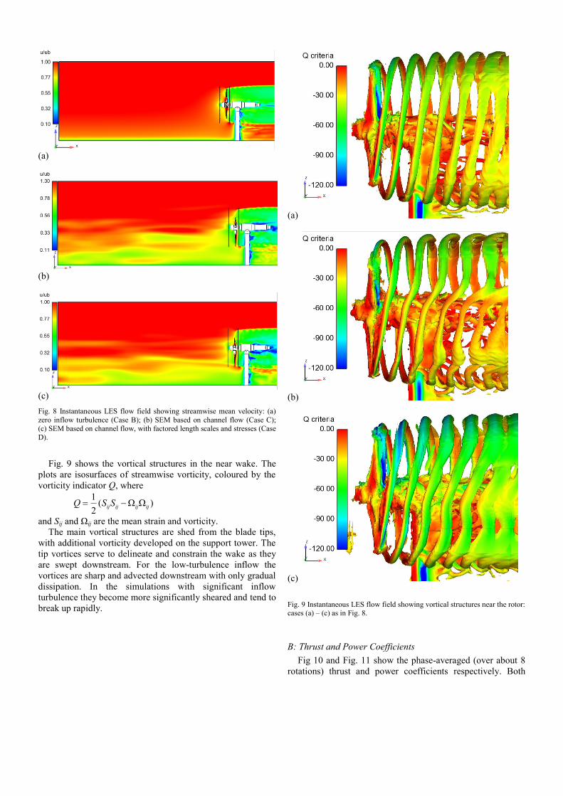
Fig. 8 Instantaneous LES flow field showing streamwise mean velocity: (a)
zero inflow turbulence (Case B); (b) SEM based on channel flow (Case C); (c) SEM based on channel flow, with factored length scales and stresses (Case
D).
Fig. 9 shows the vortical structures in the near wake. The
plots are isosurfaces of streamwise vorticity, coloured by the
vorticity indicator Q, where
)ΩΩ(2
1ijijijijSSQ
and Sij and Ωij are the mean strain and vorticity.
The main vortical structures are shed from the blade tips,
with additional vorticity developed on the support tower. The
tip vortices serve to delineate and constrain the wake as they
are swept downstream. For the low-turbulence inflow the
vortices are sharp and advected downstream with only gradual
dissipation. In the simulations with significant inflow
turbulence they become more significantly sheared and tend to
break up rapidly.
(a)
(b)
(c)
Fig. 9 Instantaneous LES flow field showing vortical structures near the rotor: cases (a) – (c) as in Fig. 8.
B: Thrust and Power Coefficients
Fig 10 and Fig. 11 show the phase-averaged (over about 8
rotations) thrust and power coefficients respectively. Both

graphs show the signature of the support tower, with three
blades passing it during each rotation and consequently
experiencing an elevated downstream pressure at these points
in the cycle. For low inflow turbulence a minimum in both
thrust and power coincides almost exactly with the passing of
a blade in front of the support tower. For the low-turbulence-
inflow cases, RANS (k-ω SST) and LES predict similar phase-
averaged thrust and power coefficients. For the latter
coefficient all computational results are slightly less than the
values obtained in the field (about 0.43 – 0.44). The various
LES simulations suggest only small effects of blade-generated
or inflow turbulence on phase-averaged load coefficients:
more significant intracycle variations and frequency spectra
are indicated below.
Fig. 10 Phase-averaged thrust coefficient.
Fig. 11 Phase-averaged power coefficient; The dashed lines indicate the range of values measured in field trials.
The degree of variation in loading for the whole rotor is
deceptively small, especially when representing the sum of
loads from three blades and phase-averaged over a number of
cycles. By contrast, Fig. 12 shows the variation in power
coefficient for one blade during a single rotation. The
coefficient has been normalised by the cycle average. In
contrast to the whole rotor, where summed contributions from
the three blades tend to smooth out variation in power
coefficient, the impact of the support tower (and a smaller
effect of velocity shear) leads to power variation for a single
blade of about 13%, with results from RANS and LES
calculations with zero turbulence at inflow being very similar.
Approach-flow turbulence introduces substantially greater
fluctuations in load, with significant implications for fatigue
damage to the blade root. Fig. 12 also shows the expected
behaviour when the turbulent lengthscales are halved at inlet,
the corresponding reduction in turbulent timescales inducing
more rapid fluctuations in load.
Fig. 12 Variation in power coefficient over one rotation (single blade,
normalised by whole-rotor average).
C: Blade Pressure Coefficient
Differences between RANS and LES simulations (with
nominally zero turbulence at inflow) are examined by plotting
the pressure coefficient on one blade at various radii. Pressure
is here normalised to the local azimuthal speed ΩR rather than
the approach-flow velocity in order to provide comparable
range over the blade radius. The negative pressure coefficient
is plotted for clarity and to emphasise lift. Fig 13 shows an
instantaneous snapshot, whilst Fig 14 shows cp values based
on average pressure over several cycles. Differences between
average pressures using RANS and LES are relatively small,
mainly being confined to the suction surface downstream of
peak suction; however, the instantaneous snapshot illustrates
the large time-varying fluctuations beyond about 50% chord
and 50% tip radius that are resolved by LES, even without
inflow turbulence.

Fig. 13 Instantaneous pressure coefficient on blade surfaces for RANS (blue) and LES (black) with nominally zero inflow turbulence.
Fig. 14 Average pressure coefficient on blade surfaces; colours as for Fig 13.
D: Load Spectra
A major objective of the present work was to compare
fluctuations in load with measurements from instrumented
blades on site. Data for this purpose was supplied by Alstom
Ocean Energy and is reported separately at this conference.
Fig. 15 shows energy spectra of flapwise bending moment
near blade root, comparing experiments, LES with zero
inflow turbulence and LES with synthetic inflow turbulence.
The frequency scale is f/f0, where f0 is the tower-passing
frequency (i.e. whole rotation) of an individual blade (about
0.2 Hz). Experimental measurements were taken at 50 Hz, so
the local spectral peak at f/f0 = 100, which corresponds to a
frequency of 20 Hz, is unexplained, but may correspond to a
natural frequency of the instrumentation or the blade.
Comparing LES simulations in Fig. 15, when there is zero
turbulence at inlet there is much less energy at frequencies
intermediate between the tower-passing frequency
(f/f0 = 1)and the high frequencies typical of blade-generated
turbulence (f/f0 > 20). When onset turbulence is included there
is much more energy in the intermediate range.
Fig. 15 Spectrum of flapwise bending moment at r/R = 0.272. Black:
experiment; green: LES with no inflow turbulence (Case B); purple: LES with turbulent inflow (Case C).
Because a relatively small number of rotations has been
sampled a more appropriate comparison with experiment is
made in Fig. 16, where spectral energy has been normalised
by variance. Only the LES with representative onset
turbulence is able to replicate the energy distribution
throughout the whole frequency range.

Fig. 16 Spectrum of flapwise bending moment at r/R = 0.272, normalised by
total variance. Colours as in Fig 15.
V. CONCLUSIONS AND FURTHER WORK
Reynolds-averaged and large-eddy simulations have been
performed for a geometry-resolved full-scale tidal-stream
turbine. Mean and fluctuating load data has been compared
with experimental measurements at the EMEC test site.
Whilst phase-averaged loads (including the influence of the
support tower) are satisfactorily reproduced by the popular
SST k-ω model, only LES with representative synthetic
turbulence at inflow is able to reproduce the full frequency
range of load fluctuations on individual blades.
Future work is under way to characterise the near-wake
structure of the flow, so that this can be input to simulations
with a second downstream rotor. This is a large step in
understanding the likely behaviour of tidal stream turbines
operating in arrays. There remains a more open-ended
aspiration to investigate the load fluctuations on turbines with
additional onset-flow variations due to waves.
ACKNOWLEDGEMENTS
The ReDAPT project was commisioned by the ETI, with
additional financial and computational support by EDF. Much
code-development work was done by Dr James McNaughton
during his PhD research. Experimental data was supplied by
the University of Edinburgh (flow) and Alstom (load).
REFERENCES
[1] Black and Veatch , “Phase II UK Tidal Stream Energy Resource
Assessment”, Rep. 107799/D/2200/03 for Carbon Trust, 2005.
[2] A.S. Bahaj, A.F. Molland, J.R. Chaplin and W.M.J. Batten , W.M.J.,
“Power and thrust measurements of marine current turbines under various hydrodynamic flow conditions in a cavitation tunnel and a
towing tank”, Renewable Energy, vol. 32, pp. 407–426, 2007.
[3] N. Barltrop, K.S. Varyani, A. Grant, D. Clelland and X.P. Pham, “Investigation into wave-current interactions in marine current
turbines”, Proc. I. Mech. E. Part A: J. Power and Energy, vol. 221, pp.
233–242, 2007. [4] E. Fernandez-Rodriguez, T.J. Stallard and P.K. Stansby, “Experimental
study of extreme thrust on a tidal stream rotor due to turbulent flow and
with opposing waves”, J. Fluids and Structures, vol. 51, pp. 354–361, 2014.
[5] T. Stallard, R. Collings, T. Feng and J. Whelan, “Interactions between
tidal turbine wakes: experimental study of a group of 3-bladed rotors”,
Phil. Trans. Roy. Soc. A: Mathematical, Physical and Engineering
Sciences, vol. 871, 2013. [6] T. Burton, N. Jenkins, G. Sharpe and E. Bossanyi, Wind Energy
Handbook, 2nd ed., Wiley, 2011.
[7] I. Afgan, J. McNaughton, D. Apsley, S. Rolfo, T. Stallard and P.K. Stansby, “Turbulent flow and loading on a tidal stream turbine by LES
and RANS”, Int. J. Heat Fluid Flow, vol. 43, pp. 96-108, 2013.
[8] M.J. Churchfield, Y. Li and P.J. Moriarty, “A large-eddy simulation study of wake propagation and power production in an array of tidal-
current turbines”, Phil. Trans. Roy. Soc. A: Mathematical, Physical and
Engineering Sciences, 871, 2013. [9] J. McNaughton, I. Afgan, D.D. Apsley, S. Rolfo, T. Stallard and P.K.
Stansby, “A simple sliding-mesh interface procedure and its
application to the CFD simulation of a tidal-stream turbine”, Int. J. Num. Meth. Fluids, vol. 74, pp. 250-269, 2014.
[10] F. Archambeau, N. Mechitoua and M. Sakiz, “Code_Saturne: a Finite-
Volume Code for the Computation of Turbulent Incompressible Flows – Industrial Applications”, Int. J. Finite Volumes, vol. 1, 2004
[11] F.R. Menter, “Two-Equation Eddy-Viscosity Turbulence Models for
Engineering Applications”, AIAA J., vol. 32, pp. 1598-1605, 1994.
[12] M. Germano, U. Piomelli, P. Moin, and W.H. Cabot, “A dynamic
subgrid-scale eddy-viscosity model”, Phys. Fluids A: Fluid Dynamics,
vol. 3, pp. 1760 – 1765, 1991. [13] D.K. Lilly, “A proposed modification of the Germano subgrid-scale
closure method”, Phys. Fluids A: Fluid Dynamics, vol. 4, pp. 633 –
635, 1992. [14] Sutherland, D.R.J., Sellar, B.G., Harding, S. and Bryden, I., “Initial
flow characterisation utilising turbine and seabed-installed acoustic sensor arrays”, in Proc. EWTEC, 2013.
[15] N. Jarrin, R. Prosser, J. Uribe, S. Benhamadouche and D. Laurence,
“Reconstruction of turbulent fluctuations for hybrid RANS/LES simulations using a synthetic-eddy method”, Int. J. Heat Fluid Flow,
vol. 30, pp. 435 – 442, 2009.