1

CFD simulations of wind distribution in an urban community

with a full-scale geometrical model

Sumei Liua, Wuxuan Pana, Hao Zhanga, Xionglei Chenga, Zhengwei Longa,*, Qingyan

Chenb,a

aTianjin Key Laboratory of Indoor Air Environmental Quality Control, School of Environmental Science

and Engineering, Tianjin University, Tianjin, China bSchool of Mechanical Engineering, Purdue University, West Lafayette, IN, USA

HIGHLIGHTS

Study of wind migration to the center of a city from a meteorological station several kilometers away.

Simulation of buildings by two different roughness setting methods. Comparison of computed wind flow with the use of a full-scale geometrical model and a

micro-scale geometrical model. Measurement of outdoor wind velocity for verification of the computed results.

ABSTRACT

A CFD study explored the use of wind information from a meteorological station to simulate wind distribution in an urban community, where the station may be located far away from the community. The study constructed a full-scale urban model with building details for the area from the meteorological station to the community. The full-scale model was typically 2 to 20 km long, which was between the micro-scale and the meso-scale model. The three-dimensional, steady Reynolds-averaged Navier-Stokes (RANS) equations was solved to simulate the urban wind flows. The investigation used two different roughness setting methods for the ground surface to approximate building structures. The two methods produced similar results, but only one of them was able to provide wind information close to the ground. The wind distribution computed by the full-scale model was compared with that computed by a micro-scale local model, where the computational domain included only building structures in the community and limited spaces in the vicinity of the community. The wind velocity computed by the full-scale model was 20% higher than the experimental data obtained by the local weather stations on a building rooftop in the community, and that computed by the micro-scale model was almost twice as much. The full-scale model is recommended for predicting wind distribution in an urban community, although more time is required for construction of the geometrical model.

Keywords: computational fluid dynamics, wind flow, full-scale model, surface roughness, buildings

1. Introduction

The investigation of wind around buildings in an urban community in the lower part of theatmospheric boundary layer (0-200 m) [1] is crucial in many wind environmental problems,

Liu, S., Pan, W., Zhang, H., Cheng, X., Long, Z., and Chen, Q. 2017. “CFD simulations of wind distribution in an urban community with a full-scale geometrical model,” Building and Environment, 117:11-23.

2

including natural ventilation design, pedestrian comfort, and air pollutant dispersion [2,3]. Solving wind environmental problems requires the study of wind flow into a community [4,5]. With the development of computing resources and grid generation techniques, an increasing number of researchers have adopted computational fluid dynamics (CFD) in their investigation of urban wind environments [6-8]. Appropriate boundary conditions are prerequisite for obtaining rational wind flow fields. CFD simulations generally use wind velocity and direction measured at a nearby meteorological station as the inflow boundary conditions.

Because of the diversity of city sizes and terrains, the variety of building heights, and the complexity of building structures, wind flow from a nearby meteorological station to a community is extremely complicated. The inhomogeneity of a city’s underlying surfaces and the high roughness arising from architectural complexes make the urban boundary layer very different from the atmospheric boundary layer on homogeneous and flat terrain, especially for the urban canopy layer (UCP) that extends from the ground to the roofs of buildings [9-11]. Using different assumptions for the urban boundary layer, researchers have developed different simulation methods [12]. These methods can be classified as meso-scale CFD models (10 – 200 km in the horizontal direction) and micro-scale model CFD models (100 m – 2 km in the horizontal direction) [13,14].

Meso-scale CFD models generally treat urban architectures as increased surface roughness to emphasize the impact of geographical and meteorological conditions on urban wind environments [15-17]. In order to describe the heterogeneity of ground cover structures reasonably well, vast studies have aimed at developing roughness parametrization methods to describe the influence of roughness elements under the UCP on the wind flow field. The parametrization methods can be classified into three categories, roughness length approaches (considering urban architectures on wind speeds and turbulence by an enhanced roughness length) [18-20], drag force parametrization (using an additional drag in the momentum equation to describe the effects of building structures on the wind flow field) [21-23], and porosity concepts (treating buildings below the UCP as porous media through which wind can pass) [12, 24, 25]. The parametrization formulas or parameters have generally been obtained by means of wind tunnel experiments in which roughness elements are simple cubes with certain distributions, whereas actual urban constructions are highly spatially inhomogeneous. It is essential to verify the methods for actual urban environments.

Micro-scale CFD models adopt large eddy simulation (LES) or Reynolds-averaged Navier-Stokes (RANS) turbulence models to study wind flow around isolated building or architectural complexes. Those models explicitly construct building details on a local scale [26-28]. The wind velocity and direction from the nearest meteorological station are used as boundary conditions. The impact of city buildings on upstream flow is modified by roughness length. In the vertical direction, the wind profile is generally described as a logarithmic law or power law [29-31]. As this kind of method neglects the effect of buildings structures on the upstream flow, it is applicable only where Monin-Obukhov similarity holds, such as in a suburban district with flat terrain [32, 33].

Previous studies of meso-scale or micro-scale models have not determined how to correctly consider the influence of inhomogeneous building complexes in intermediate terrain between a community site in a city and a meteorological station that could be several kilometers away. Our investigation examined methods of simulating urban terrains with the use of roughness. Our goal was to find a suitable geometrical model with appropriate boundary conditions that could calculate wind distribution at a community site with reasonable accuracy. The accuracy was verified with measured data from the field. This paper reports the results that were obtained.

3

2. Research Method

2.1 CFD model

This investigation used a geometrical model that combines elements of both meso-scale and micro-scale models. The geometrical model is the same as a micro-scale model with explicitly constructed building details, but the computational domain extends from the community site to a weather station several kilometers away. The domain is much larger than that used by a micro-scale model, which incorporates a small computational domain around the community site. The full-scale model was typically 2 to 20 km long, which was between the micro-scale and the meso-scale model. Thus, we call this a full-scale model that differs from the micro-scale model only in the computational domain size.

Our study was based on recommendations from the overview of CFD use in simulating the outdoor environment by Blocken, et al. [34], from “Best practice guideline for the CFD simulation of flows in the urban environment” [35], and from “Architectural Institute of Japan (AIJ) guidelines for practical applications of CFD to pedestrian wind environment around buildings” [36]. These simulations were conducted with the use of a commercial CFD program, ANSYS Fluent 14.0 [37]. The CFD model used in this program solves the Reynolds-averaged Navier-Stokes (RANS) equations with the re-normalization group (RNG) k- turbulence model. The model performed well in simulations of urban wind flows [38, 39]. In the RNG k-ε model, the transport equations of turbulence kinetic energy k and its dissipation rate are:

(1)

1 ⁄

1 (2)

where ρ is air density (kg/m3), t time (s), and the Reynolds time-averaged velocity

component in the xi and xj (i, j =1, 2, 3) directions, respectively, the dynamic viscosity of

air (m2/s), the turbulence kinematic viscosity (m2/s), 0.7194 the turbulence

effective Prandtl number for k, G the source term, 0.7194 the turbulence effective

Prandtl number for ε, 1.42 , 1.68 , 0.085 , η 2 ∙ / ,

, β 0.012, and 4.38.

2.2 Computational domain size and mesh generation

The computational domain for a micro-scale model typically includes the community site concerned and its immediate surroundings. The micro-scale model has a mature theory about the best way to determine the vertical, lateral, and flow direction domains. For the height of the computational domain, the blockage ratio should be below 3% [35, 36]. The boundary in the four horizontal directions should be a distance of at least 5Hmax [35, 40] to allow for the establishment of a realistic flow behind the wake region [35, 36, 41]. To eliminate as far as possible the errors caused by the size of the computational domain, for the micro-scale model we used a distance of 15Hmax beyond the community site in four directions and blockage ratio should be below 3% for the height of the computational domain, as shown in Fig. 1(b). The

4

micro-scale model was not the focus of this investigation, but rather it was used as a reference.

(a) (b) Fig.1. Computational domain and boundary conditions for (a) the full-scale model and (b) the micro-scale model.

Our full-scale model used the nearest weather station as the inflow boundary of the

computational domain. The boundary in the downstream region and the lateral boundaries were at a distance of 15Hmax from the community site, and blockage ratio should be below 3% for the height of the computational domain. Fig. 1(a) is a sketch of the computational domain. Note that Hmax may differ between the full-scale and micro-scale models, because the tallest building in the full-scale model could be higher than that in the micro-scale model. In the central computational domain, inhomogeneous building complexes were elaborately constructed. This central domain included not only the community site concerned, but also at least one additional street block in each lateral direction around the community [36]. In the outer regions in the lateral directions and on the downstream side of the central domain, the building geometry can be simplified as roughness, which will be discussed in Section 2.3.

Gambit 2.4.6 was used to generate a discrete grid in this study. Because of the complexity of the geometrical model, this study used a hybrid grid scheme with a tetrahedral grid, which can adapt to the geometric structures very well. In the central region, building structures were explicitly constructed, while on the two sides, no geometric configurations were established.

2.3 Boundary conditions

The mean velocity profile for the inflow boundary was modeled as a power law, as shown in Eq. (3). For the full-scale model, the inflow boundary was specified as the weather station location, whereas for the micro-scale model, the wind velocity profile was modified to consider the impact of the terrain. The downstream vertical boundary was modeled as outflow. The sky was treated as a mirror plane. For the ground surface, the standard wall functions with a roughness modification based on the equivalent sand-grain roughness height ks and the roughness constant Cs were used to reflect the influence of roughness elements, such as buildings and trees, on the urban wind flow field [37]. The surfaces of the buildings in the computational domain were non-slip.

5

The wind information provided by a weather station is the mean velocity at a reference height over a period of one hour, and therefore the inlet boundary conditions can be determined by

(3)

where Uz is the mean velocity profile (m/s), Ur the velocity (m/s) at reference height zr (m), and a power law exponent determined by the terrain category.

For the ground, the wall functions are based on the universal near-wall velocity distribution (law of the wall) modified for a rough surface [37]:

∗ 1

ln∗

Δ (4)

where is the tangential wind speed in the center (point P) of the wall-adjacent cell (m/s),

∗ is the wall function friction velocity (m/s) with constant = 0.085, the wall function friction velocity (m/s), the von Karman constant (~ 0.42), E an empirical constant for a smooth wall (≈ 9.793), the distance from the center of the wall-adjacent cell to the wall (m), and the dynamic viscosity (N•s/m2). The term ΔB hinges on the type and size of the roughness elements and has been found to be closely correlated with the roughness Reynolds number, ks

+=ρksu*/μ, where ks is the physical roughness height. For a fully developed atmospheric boundary layer profile, the vertical profile for the mean

wind speed has the following form [42]:

∗

1ln (5)

where is the wind speed at a height of z (m/s), z is the height (m), ∗ the friction velocity of the atmospheric boundary layer (m/s), and z0 the aerodynamic roughness length (m) that is equivalent to the height at which the wind speed theoretically becomes zero. Table 1 shows the z0 values for different terrains [1, 43]. Table 1 Roughness values for different terrains [1, 43]

Type z0 (m)

Smooth wall 0 Grass land 0.03 Few isolated obstacles 0.05

Low crops / Occasional large obstacles 0.1 Parkland / Shrubs / Numerous obstacles 0.5

Densely distributed mid-rise and high-rise buildings / Clumps of forest

1

The combination of Eqs. (4) and (5) yields [1]:

9.793 (6)

6

This equation can be used to describe z0 in order to take into account the influence of

roughness elements on the wind flow field. As it is very time consuming to build the flow domain with full building details on the

ground, the micro-scale and full-scale models divide the ground surface into two parts. One part is the central region with building details, apart from some relatively small buildings and trees that have been omitted. The other part is the perimeter of the micro-scale model or the two sides of the full-scale model that do not have building structures, as shown in Fig. 1.

For the central region with building details, the roughness value of the ground surface is z0

= 0.03 m according to Table 1. However, for the part of the ground surface without building structures, a roughness value of z0 = 1 m should be used. This investigation aimed to compare two kinds of roughness setting methods for the ground surface, (1) change in Cs while keeping ks = 1 and (2) change in ks while keeping Cs = 1 for desirable values of z0.

2.4 Field measurements for CFD validation

Validation of CFD simulations with experimental data is essential. This study calculated wind flow for an urban community by using wind information from a meteorological station. For validation purposes, several HOBO micro weather stations were used to measure the wind velocity magnitude inside the community site from August 15, 2016 to October 31, 2016. The measurement locations were 2 m above the roof of one of the buildings. The frequency of the measured data was collected every minute. The measured data was averaged hourly for consistency with hourly data acquired from the meteorological station. The micro weather stations had a measuring accuracy of ±0.4% for wind velocity if it was greater than 0.5 m/s.

3. Case setup

3.1 Geometrical models

To compare the performance of the full-scale model with the micro-scale model, this study selected Tianjin City in China as an example. We selected this city for our convenience. The city has an urban population of 5.21 million and urban structures that are typical of large cities in China. Since Tianjin University is close to the downtown area, this investigation chose a 1.05 km x 1.05 km section of the Tianjin University campus as the community site, as shown in Fig. 2(a). Tianjin has 12 meteorological stations scattered in and around the city [44] at distances of 10 km to 100 km from the university campus. The further a meteorological station is from the campus, the less reliably does weather data at the station reflect that on the campus. This study selected the closest meteorological station, Xiqing station, to provide hourly wind velocity and wind direction. This station is located 10 km from the campus in the west-west-south (WWS) direction.

7

(a)

(b)

(c) (d)

Fig. 2. Geometrical models used in this study: (a) plane view of the topographical information from Xiqing meteorological station (the star to the community site (the square), (b) building details used in the full-scale model, (c) computational domain of the full-scale model, and (d) computational domain of the micro-scale model with building details in the center.

Fig. 2(a) shows the geographical location of the Xiqing station (the large star at the lower left) in relation to the community site (the square at the upper right) on a Google satellite map. Fig. 2(b) illustrates the constructed three-dimensional geometrical model from the Xiqing station to the site. The model was 10.8 km long and 1.8 km wide (encompassing at least one additional street block in each direction around Tianjin University, as discussed in Section 2.2). All buildings inside this area were explicitly resolved, while other structures, such as trees, landscaping, roads, etc., were neglected in the model. The corresponding

8

computational domain was extended by 1.8 km or about 15Hmax on both sides and at the right end, where the tallest building in the area was 117 m high. The resulting computational domain was 12.6 km long, 5.4 km wide, and 0.351 km high. The maximum blockage ratio was 1.5%, as shown in Fig. 2(c). The use of the outer regions would reduce the amount of labor-intensive work required for constructing the detailed building structures, if they could be approximated by roughness.

For comparison, this study also built a micro-scale model as shown in Fig. 2(d). The height of the computational domain was 105 m or three times the height of the tallest building (35 m) inside this area. The other four directions were extended by a distance of 15 x 35 = 525 m. Therefore, the computational domain for the micro-scale model was 2.1 km long, 2.1 km wide, and 0.105 km high. The maximum blockage ratio was 2.4%.

3.2 Grid arrangement and mesh generation

Mesh quality is very important for the accuracy of simulation results. There were 3,637 buildings scattered throughout the inner region of the full-scale model, and the building heights ranged from 3 m to 117 m. As shown in Fig. 3(a), this study divided the inner region into 69 sub-regions according to building height and density. Streets and community fences were usually used as partition lines. The mesh was first generated for each sub-region and then combined for the whole domain. Because of our limited computing capacity and the possible impact of grid size on accuracy, the maximum grid size was 20 m near the Xiqing meteorological station area and was gradually reduced to 8 m at the community site in the lengthwise direction. The maximum grid size in the vertical direction was 10 m. The grid resolution along the perimeter without buildings was 20 m. The result was a total grid number of 7.0 million for the full-scale model of Fig. 2(c). Fig. 3(b) shows the grid cells generated on the building surfaces and in the area without building details for the top right corner in Fig. 3(a), with triangular and quadrilateral mesh. The mesh for the micro-scale model was similar to that for the full-scale model, with the use of a hybrid grid scheme with a tetrahedral grid in the central area where building structures were explicitly constructed and a hexahedral grid at the perimeter where there were no geometric details. The maximum grid sizes of the inner region and in the perimeter area were 4 m and 6 m, respectively, and the total grid number was 6.4 million.

9

(a)

(b)

Fig. 3. Grid generation for the full-scale model: (a) sub-regions and (b) grid cells on the building surfaces and in the perimeter zone without building details.

3.3 Boundary conditions and case setup

This investigation used the average wind velocity and direction measured at the Xiqing meteorological station from 11:00 am to 2:00 pm on August 30, 2016, as the boundary conditions when the wind angles on the hour were 229°, 230°, 221°, 232°, respectively. The wind direction was southwest and the wind speed was 2.6 m/s. Thus, the western and southern boundaries were inflow ones. Because the Xiqing station was in a suburb, a power law with an exponent of 0.22 (as shown in Eq. (3)) was used to specify the vertical wind profile [45] at the two inlet boundaries in CFD simulations with the full-scale model, which corresponds z0=1 m. For the micro-scale model, the exponent was changed to 0.3 to reflect the change from a suburb to a more built-up area, which corresponds z0=0.3 m. The sky of the domain was modeled as a symmetrical surface or as a mirror. The outlet boundary conditions on the eastern and northern boundaries were set at zero static pressure. The wall functions with the roughness values were used for the ground surfaces.

As discussed in the previous section, there were two roughness setting methods. This investigation aimed to identify the better method. As shown in Table 2, Case 01 used a smooth wall boundary for the ground surface as a benchmark case to be compared with the other cases with using wall functions to illustrate the influence of roughness elements on the wind flow field. Eight cases were then set up to compare the effects of changing Cs or ks

10

according to Eq. (8), which also led to different values of z0. In these cases, we changed only one parameter at a time in simulations of the wind distribution with the full-scale model.

Table 2 Case setup for different terrains (z0) under different combination of ks and Cs.

Outer regions without building details (EX)

Inner region with buildings details (IN)

Cases ks Cs z0 (m) ks Cs z0 (m)

Case 01 0 0.5 0 0 0.5 0 Case 02

1

0.5 0.05

0 0.5 0

Case 03 1 0.1 Case 04 4.897 0.5 Case 05 9.793 1 Case 06 0.5

1

0.05 Case 07 1 0.1 Case 08 4.897 0.5 Case 09 9.793 1 Case 10

0 0.5 0 0.59 0.5

0.03 Case 11 0.5 0.59 Case 12 1 9.793

1 0.59 0.5 0.03 Case 13 9.793 1

Cases 02 to 05 assumed ks = 1 and varied Cs for different z0 in the outer regions without

building details, while z0 for the inner region remained at zero. This investigation focused more on the outer regions because there were no building details, and the impact of the roughness setting on the wind flow could be easily studied. Cases 06 to 09 kept Cs at 1 and varied ks for different z0 in the outer regions. These cases were used to assess the two roughness setting methods.

Cases 10 and 11 changed z0 to 0.03 (compared to z0 = 0 in the reference case) with the two different methods, while the roughness in the outer regions was assumed to be zero. Finally, Cases 12 and 13 changed z0 to 1 for the outer regions.

Evaluation of these cases allowed us to identify a suitable roughness setting method for the full-scale model. We could then compare the performance of the full-scale model with that of the micro-scale model.

3.4. Other computational parameters

The governing equations are solved using the finite volume method. The SIMPLE algorithm was used for pressure and velocity coupling, and the second-order discretization schemes were used for solving all the variables. When the scaled residuals reached 10-4 for mass conservation, U, V, W, k, the solution is considered to be converged. Velocity magnitude on several specified points were also monitored to confirm that the solution does not change with the iteration, which is another criterion for convergence.

11

3.5. Field measurements

Field measurements were conducted at Tianjin University with three HOBO micro weather stations positioned on the rooftop of a building as shown in Fig. 4. The building height was 9 m, and the sensor height was 11 m above the ground.

(a)

(b)

Fig. 4. Three measurement positions on the rooftop of a campus building: (a) sensor locations and (b) building location at the university site.

4. Results

4.1 Model validation

This investigation first validated the CFD models by comparing our simulated results with wind tunnel data from the literature. The wind tunnel data had been collected at an urban complex in Niigata, Japan, with a scale of 1:250 [46]. Scalar wind velocities were measured at a height of 8 mm above the wind tunnel floor (corresponding to a height of 2 m above the ground in actual scale) by multi-point thermister anemometers. Fig. 5(a) shows the building model of the urban area in the actual scale of 500 m long, 500 m wide, and 300 m high. A hybrid grid type was used in this study, with a tetrahedral grid in the inner area with building structures and a hexahedral grid in the outer regions. The total grid number was 5.6 million, as shown in Fig. 5(b). Table 3 lists the boundary conditions used in this investigation.

(a) (b)

Fig.5. (a) Geometric configuration of the urban area used for the CFD validation and (b) the grid built for the CFD simulations.

P1

P2 P3

12

Table 3 Boundary conditions used in this study.

Inlet flow boundary Interpolated values of velocity and turbulence kinetic energy from experimental data for the inflow, ＝CD

1/2･k･dU/dz（ ＝Pk） Outflow boundary Outflow with zero pressure Top surface Solid mirror wall Ground surface Logarithmic law with roughness length z0 = 0.024 m Building surfaces Logarithmic law for smooth walls

In the wind tunnel case, the micro-scale model is the same as the full-scale model.

Therefore, the experimental data from the wind tunnel was used to validate aspects of the physical model such as the turbulence model, numerical algorithm, etc. The RNG k- model was used to simulate the urban wind flow, the SIMPLE algorithm was used for pressure and velocity coupling, and second-order discretization schemes were used for the governing equations.

Fig. 6(a) compares the wind speed ratio (defined as the ratio of the wind speed magnitude at each measuring point and the wind speed at the same height at the inflow boundary) computed in selected locations at a height of 8 mm above the wind tunnel floor with the corresponding experimental data. The mean relative error of our calculation was 36.4%. As a comparison, Fig. 6(b) shows the computed results from Yoshihide et al. [48] with the same experimental data. Although Yoshihide et al. did not show the quantitative error, the two computed results were similar. The comparisons indicate that the RNG k- model and numerical algorithm can predict the airflow in an urban area reasonably well, considering the complexity of the geometry and wind flow.

(a)

(b)

Fig. 6. Comparison of the normalized wind speed computed by the RNG k- model with the measured data from the wind tunnel [46] at selected locations (a) between the present study and the data, and (b) between the study from Yoshihide et al. [46] and the data.

13

4.2 Grid-independence analysis

A mesh independence study was conducted for the micro-scale model and full-scale model. Figure 7(a) shows the computed vertical wind profiles with different grid number for the micro-scale model. The results show that the 1.4 million grid was sufficiently good for the micro-scale model. This study used the 6.4 million grid for the subsequent simulations. Figures 7(b), (c) and (d) show the computed vertical wind profiles with different grid numbers for the full-scale model in the windward outer region, inner region, and leeward outer region. The 7.0 million grid can produce a grid-independent result.

(a) (b) (c) (d)

Fig. 7. Computed wind profiles with different grid number: (a) surface averaged velocity for micro-scale model, (b) averaged in the windward outer region for the full-scale model, (c) averaged in the inner region for the full-scale model, and (d) averaged in the leeward outer region for the full-scale model.

4.3 Comparison of different methods in specifying roughness parameters

With the validated turbulence model, this investigation used the full-scale geometrical model to determine the wind distribution on the university campus. As discussed in the case setup section, it is important to study the impact of different z0 values on the wind profile in the outer regions without building details. Case 01 was a reference case with a smooth ground surface (z0 = 0). The z0 for Cases 02 to 05 increased in the outer regions, while smooth ground was assumed in the inner region. In the outer regions, different z0 values were achieved by varying Cs while keeping ks = 1. Fig. 8 shows the computed vertical wind profile along the height in three different regions: the windward outer region, inner region, and leeward outer region. With an increase in Cs or z0, the wind velocity near the ground in the two outer regions decreased dramatically, while that in the inner region remained the same. The results look plausible, as a larger roughness length would create a high resistance and reduce the wind velocity near the ground. These results have verified the possibility of achieving different z0 values by changing Cs.

14

(a) (b) (c) Fig. 8. Computed wind profiles with different z0 by varying Cs and keeping ks = 1: (a) averaged in the windward outer region, (b) averaged in the inner region, and (c) averaged in the leeward outer region.

This investigation also simulated the wind profiles by varying ks for different z0 while

keeping Cs constant from Case 06 to Case 09 as shown on Table 2. Fig. 9 compares the wind profiles for Cases 02 to 05 with those for Cases 06 to 09. When the roughness was small, the two methods for the same z0, such as Cases 02 and 06, yielded nearly the same results. With the largest z0 value of 1, the difference between the two roughness setting methods was 11.6% for the air velocity near the ground.

15

(a) (b) (c)

Fig. 9. Comparison of the computed wind profiles with different z0 by varying Cs and keeping ks = 1 for Cases 02 to 06 or by varying ks and keeping Cs = 1: (a) averaged in the windward outer region, (b) averaged in the inner region, and (c) averaged in the leeward outer region.

According to Eq. (8), any combination of ks and Cs with the same product can be used. ANSYS Fluent requires ks < zp where zp is the distance from the center (point p) of the wall-adjacent cell to the wall surface [47] and the default maximum Cs is 1. When z0 = 1 and Cs = 1 as in Case 09, then ks = 9.793, which requires a minimum first grid size near the ground of 2 x 9.793 = 19.586 m. If information close to the ground was desired, such as the wind speed at pedestrian level, this method of setting roughness would not produce the necessary information. Thus, changing Cs is better than changing ks.

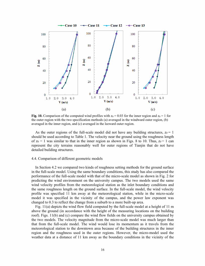
We designed Cases 10 and 11 to study the impact of the two roughness setting methods in the inner region with z0 = 0.03. As shown in Fig. 10, the difference was as small as 0.6%. Maintaining the z0 value in the inner region at 0.03, we studied the two different roughness setting methods for z0 = 1 in the outer regions (Cases 12 and 13). The methods again differed by 11.6% as illustrated in Fig. 10. This result implies that the impact of roughness in the inner region on the velocity profile in the outer regions was small. The velocity profiles in the outer regions depended only on the roughness in these regions.

16

(a) (b) (c)

Fig. 10. Comparison of the computed wind profiles with z0 = 0.03 for the inner region and z0 = 1 for the outer region with the two specification methods (a) averaged in the windward outer region, (b) averaged in the inner region, and (c) averaged in the leeward outer region.

As the outer regions of the full-scale model did not have any building structures, z0 = 1

should be used according to Table 1. The velocity near the ground using the roughness length of z0 = 1 was similar to that in the inner region as shown in Figs. 8 to 10. Thus, z0 = 1 can represent the city terrains reasonably well for outer regions of Tianjin that do not have detailed building structures.

4.4. Comparison of different geometric models

In Section 4.2 we compared two kinds of roughness setting methods for the ground surface in the full-scale model. Using the same boundary conditions, this study has also compared the performance of the full-scale model with that of the micro-scale model as shown in Fig. 2 for predicting the wind environment on the university campus. The two models used the same wind velocity profiles from the meteorological station as the inlet boundary conditions and the same roughness length on the ground surface. In the full-scale model, the wind velocity profile was specified 11 km away at the meteorological station, while in the micro-scale model it was specified in the vicinity of the campus, and the power law exponent was changed to 0.3 to reflect the change from a suburb to a more built-up area.

Fig. 11(a) depicts the wind flow field computed by the full-scale model at a height of 11 m above the ground (in accordance with the height of the measuring locations on the building roof). Figs. 11(b) and (c) compare the wind flow fields on the university campus obtained by the two models. The velocity magnitude from the micro-scale model was much larger than that from the full-scale model. The wind would lose its momentum as it travels from the meteorological station to the downtown area because of the building structures in the inner region and the roughness used in the outer regions. However, the micro-model used the weather data at a distance of 11 km away as the boundary conditions in the vicinity of the

17

campus even though the power law exponent was changed. The results clearly indicate that the two models did not perform similarly.

(a)

(b) (c)

Fig. 11. Comparison of the performance of the two geometrical models: (a) wind flow field computed by the full-scale model, (b) the wind on the university campus computed by the full-scale model, and (c) the wind on the campus computed by the micro-scale model.

Fig. 12 compares the simulated wind velocity with the corresponding experimental data at

the rooftop locations in Fig. 4. Although the data points from the experiment were limited, the trend is clear. The results show that the micro-scale model significantly overestimated the wind magnitude. This occurred because the model failed to consider the decay in velocity as the wind traveled through the city from the meteorological station. The results obtained by the full-scale model were in reasonable agreement with the measured data. The simulations with the two roughness setting methods for the full-scale model again generated similar accuracy at this height. Nevertheless, the full-scale model overestimated the wind velocity by 20%. This could be due to our underestimation of the roughness in the inner region. We can conclude from the comparison that the full-scale model performed much better than the micro-scale model.

18

Fig. 12. Comparison of the results simulated by the full-scale model and micro-scale model with the wind velocity measured on the roof of a building on the campus.

5. Discussion

The full-scale model performed quite well for such a complex case study. However, the model had some limitations: The full-scale geometrical model was established with the aid of a satellite image

because no public geometrical model was available. The model used approximations that may have affected the wind profiles. We were unable to estimate the errors that may have resulted.

This investigation selected the Xiqing meteorological station, which was the closest to the university campus. The simulations used wind data from the direction upwind from the meteorological station as the boundary conditions. If the wind came from a different direction, such as from the university campus to the meteorological station, could the wind data from the station be used as the inlet boundary conditions? To use wind data from the upwind direction, we would need to build a new full-scale geometrical model. The effort would be significant.

This study used the RNG k- model to simulate the urban wind flow under steady-state conditions. However, wind constantly changes in direction and magnitude. Should a transient simulation method be used, it would significantly increase the computing costs.

6. Conclusions

This investigation conducted CFD simulations to compare different geometrical models and roughness setting methods for simulating the wind environment in an urban community. The study led to the following conclusions:

The micro-scale model predicted the wind distribution for a community with boundary conditions from a wind tunnel with a relative error of 36.4% compared with experimental data from the literature. Our simulation accuracy appeared to be similar to that obtained by the group who did the wind tunnel tests.

This study tested two different roughness setting methods, and both produced satisfactory wind profiles for outer regions without building details. It is better to vary

19

Cs while keeping ks = 1 because the method can be used to calculate wind distribution close to the ground.

The full-scale model was able to produce the wind velocity distribution in the community by using wind information from a meteorological station that was 11 km away. It overestimated the wind velocity by only 20% compared with the measured data obtained on the rooftop of a building in the community site. If the wind information was used for the micro-scale model, the model would overestimate the wind velocity by a factor of two. This is because the model did not consider the wind decay when it traveled through the city, even though the exponent on the wind profile was modified for the city terrain.

Acknowledgement

The authors would like to thank Prof. Yoshihide Tominaga of Niigata Institute of Technology, Japan, for providing us with the wind tunnel data and further explanation of the data. The authors are also in debt to Prof. Bert Blocken of Eindhoven University of Technology, The Netherlands, for his help with boundary-layer theory.

Funding

The research presented in this paper was partially supported by the National Natural Science Foundation of China through Grant No. 51678395 and by the national key project of the Ministry of Science and Technology, China, on “Green Buildings and Building Industrialization” through Grant No. 2016YFC0700500.

References

[1] Blocken, B., Stathopoulos T., Carmeliet J. CFD simulation of the atmospheric boundary layer: Wall function problems. Atmospheric Environment, 41 (2007) 238-252.

[2] Blocken, B. Computational Fluid Dynamics for urban physics: Importance, scales, possibilities, limitations and ten tips and tricks towards accurate and reliable simulations. Building and Environment, (2015) 91, 219-245.

[3] Razak, AA., Hagishima, A., Salim, SAZS. Progress in wind environment and outdoor air ventilation at pedestrian level in urban area. Applied Mechanics & Materials, 819 (2016) 236-240.

[4] Yukio, T., and Ryuichiro, Y. 2016. Advanced environmental wind engineering. Japan. [5] Willemsen, E., and Wisse, JA. Design for wind comfort in the Netherlands: Procedures, criteria and

open research issues. Journal of Wind Engineering and Industrial Aerodynamics, 95 (2007) 1541–1550.

[6] Chen, Q. “Chapter 7: Design of natural ventilation with CFD,” Sustainable Urban Housing in China, Edited by L.R. Glicksman and J. Lin, Springer. 2006, pp. 116-123.

[7] Ramponi, R., Blocken, B., Coo, LBD., et al. CFD simulation of outdoor ventilation of generic urban configurations with different urban densities and equal and unequal street widths. Building and Environment, 92 (2015) 152-166.

[8] Jin, M., Zuo, W., and Chen, Q. Simulating natural ventilation in and around buildings by fast fluid dynamics. Numerical Heat Transfer, Part A: Applications, 64(4) (2013) 273-289

[9] Oke, TR. Boundary Layer Climate. London, Methuan & Co. LTD. (1987) 274. [10] Harman, IN., and Finnigan, JJ. A simple unified theory for flow in the canopy and roughness sublayer.

Boundary-Layer Meteorol, 123 (2007) 339–363. [11] Stull, RB. An introduction to boundary layer meteorology. Canada, Kluwer Academic Publishers,

105(3) (1988) 515-520. [12] Crago, RD., Okello, W., Jasinski, MF. Equations for the drag force and aerodynamic roughness length

of urban areas with random building heights. Boundary-Layer Meteorology, 145 (2012) 423-437.

20

[13] Hang, J., Li, YG. Wind conditions in idealized building clusters: Macroscopic simulations using a porous turbulence model. Boundary-Layer Meteorology, 136 (2010) 129-159.

[14] Britter, RE., Hanna, SR. Flow and dispersion in urban areas. Annual Review of Fluid Mechanics, 35 (2003) 469-496.

[15] Liu, HP., Zhang, BY., Sang, JG., et al. A laboratory simulation of plume dispersion in stratified atmospheres over complex terrain. Journal of Wind Engineering & Industrial Aerodynamics, 89(1) (2001) 1–15.

[16] Ding, AJ., Wang, T., Zhao, M., et al. Simulation of sea-land breezes and a discussion of their implications on the transport of air pollution during a multi-day ozone episode in the Pearl River Delta of China. Atmospheric Environment, 38(39) (2004) 6737-6750.

[17] Tong, H., Walton, A., Sang, JG., et al. Numerical simulation of the urban boundary layer over the complex terrain of Hong Kong. Atmospheric Environment, 39(19) (2005) 3549-3563

[18] Ng, E., Yuan, C., Chen L., et al. Improving the wind environment in high-density cities by understanding urban morphology and surface roughness: A study in Hong Kong. Landscape and Urban Planning, 101 (2011) 59-74.

[19] Kim, BG., Lee, CH., Joo, SJ., et al. Estimation of roughness parameters within sparse urban-like obstacle arrays. Boundary-Layer Meteorology, 139 (2011) 457-485.

[20] Cao, MC., Lin, ZH. Impact of urban surface roughness length parameterization scheme on urban atmospheric environment simulation. Journal of Applied Mathematics, 12(2) (2014) 155-175.

[21] Coceal, O., Belcher, SE. A canopy model of mean winds through urban areas. Quarterly Journal of Royal Meteorological Society, 130 (2004) 1349-1372.

[22] Sabatino, SD., Solazzo, E., Paradisi, P. A simple model for spatially-averaged wind profiles within and above an urban canopy. Boundary-Layer Meteorology, 127 (2008) 131-151.

[23] Peng, Z., Sun, J. Characteristics of the drag coefficient in the roughness sublayer over a complex urban surface. Boundary-Layer Meteorology, 153 (2014) 569-580.

[24] Skote, M., Sandberg, M., Westerberg, U., et al. Numerical and experimental studies of wind environment in an urban morphology. Atmospheric Environment, 39 (2005) 6147-6158.

[25] Kuwahara, F., Yamane, I., Nakayama, A. Large eddy simulation of turbulent flow in porous media. International Communications in Heat and Mass Transfer, 33(4) (2006) 411-418.

[26] Li, Y., Stathopoulos, T. Numerical evaluation of wind-induced dispersion of pollutants around a building. Journal of Wind Engineering & Industrial Aerodynamics, 67 (1997) 757-766.

[27] Martilli, A., Santiago, JL. CFD simulation of airflow over a regular array of cubes. Part II: Analysis of spatial average properties. Boundary-Layer Meteorology. 122(3) (2007) 635-654.

[28] Santiago, JL., Martilli, A., Martin, F. CFD simulation of airflow over a regular array of cubes. Part I: Three-dimensional simulation of the flow and validation with wind-tunnel measurements. Boundary Layer Meteorology, 122(3) (2007) 609-634.

[29] Montazeri, H., Blocken, B. CFD simulation of wind-induced pressure coefficients on buildings with and without balconies: Validation and sensitivity analysis. Building and Environment, 60 (2013) 137-149.

[30] Liu, SM., Liu, JJ., Yang, QX., et al. Coupled simulation of natural ventilation and daylighting for a residential community design. Energy and Buildings, 68 (2014) 686-695.

[31] Santiago, JL., Coceal, O., Martilli, A., et al. Variation of the sectional drag coefficient of a group of buildings with packing density. Boundary-Layer Meteorology, 128(3) (2008) 445-457.

[32] Solazzo, E., Sabatino, SD., Aquilina, N., et al. Coupling mesoscale modelling with a simple urban model: The Lisbon case study. Boundary-Layer Meteorology, 137 (2010) 441-457.

[33] Barlow, JF., Rooney, GG. Hünerbein, SV., et al. Relating urban surface-layer structure to upwind terrain for the Salford experiment (Salfex). Boundary-Layer Meteorology, 127 (2008) 173-191.

[34] Blocken, B., Stathopoulos T., Carmeliet J., et al. Application of CFD in building performance simulation for the outdoor environment: An overview. Journal of Build Performance Simulation, 4(2) (2011) 157-84.

[35] Jörg, F., Alexander, B. Best practice guideline for the CFD simulation of flows in the urban environment: COST action 732 quality assurance and improvement of microscale meteorological models. Brussels, COST Office. 2007.

[36] Tominaga, Y., Mochida, A., Yoshie, R., et al. AIJ guidelines for practical applications of CFD to pedestrian wind environment around buildings. Journal of Wind Engineering and Industrial Aerodynamics, 96 (2008) 1749-1761.

[37] ANSYS Inc.. ANSYS Fluent 14.0 user’s guide. ANSYS Inc. Southpointe. 2011.

21

[38] Ferreira, AD., Sousa, ACM., Viegas, DX. Prediction of building interference effects on pedestrian level comfort. Original Research Article Journal of Wind Engineering and Industrial Aerodynamics, 90 (4-5) (2002) 305–319.

[39] Zhang, AX., Gao, CL., Zhang, L. Numerical simulation of the windfield around different building arrangements. Original Research Article Journal of Wind Engineering and Industrial Aerodynamics, 93 (12) (2005) 891–904.

[40] Scaperdas, A. and Gilham, S. Thematic Area 4: Best practice advice for civil construction and HVAC. The QNET-CFD Network Newsletter, 2(4) (2004) 28-33.

[41] Bartzis, J.G., Vlachogiannis, D., and Sfetsos, A. Thematic Area 5: Best practice advice for environmental flow. The QNET-CFD Network Newsletter, 2(4) (2004) 34-39.

[42] Durbin, P.A., Petterson Reif, B.A., Statistical theory and modelling for turbulent flows. Wiley, Chichester, UK. 2001.

[43] Wieringa, J. Updating the Davenport roughness classification. Journal of Wind Engineering and Industrial Aerodynamics, 41(1-3) (1992) 357-368.

[44] http://data.cma.cn/ [45] Gu, JX. Dictionary of atmospheric science. Beijing, China Meteorological Press, (1994) 156. [46] Tominaga, Y., Yoshie, R., Mochida, A., et al. Cross comparisons of CFD prediction for wind

environment at pedestrian level around buildings, Part 2: Comparison of results for flowfield around building complex in actual urban area. The Sixth Asia-Pacific Conference on Wind Engineering (APCWE-VI) Seoul, Korea, September 12-14. 2005.

[47] Blocken, B., Carmeliet, J., Stathopoulos, T. CFD evaluation of wind speed conditions in passages between parallel buildings—effect of wall-function roughness modifications for the atmospheric boundary layer flow. Journal of Wind Engineering and Industrial Aerodynamics, 95 (2007) 941–962.