CFD Validation of Synthetic Jets And Turbulent Separation Control

Volume 1

Contributed Papers

Langley Research Center Workshop

CFD Validation of Synthetic Jets and Turbulent Separation Control

In association with

Case 1: Synthetic Jet

into Quiescent Air Case 2: Synthetic Jet in a

Crossflow Case 3: Flow over a Hump Model (Actuator

Control)

March 29-31, 2004

Woodlands Hotel and Conference Center Colonial Williamsburg

Williamsburg, Virginia, USA

Local Organization: Thomas Gatski, Christopher Rumsey

Table of Contents

Case 1

Contribution Page

Description of Experiment…...……………….……………………………….... 1.1

Submission Details and Guidelines………………….………………………….. 1.2

Numerical Simulation of a Synthetic Jet into a Quiescent Air……….………… 1.3 Simulation of a Synthetic Jet in Quiescent Air Using TLNS3D Flow Code…… 1.4

Synthetic Jet Into Quiescent Air.URANS Simulations with Eddy-Viscosity and Reynolds-Stress Models ………………………………………………………… 1.5

Cubic and EASM Modelling of Synthetic Jets…………………………………. 1.6

Numerical Simulation of a Synthetic Jet into a Quiescent Air Using a Structured and an Unstructured Grid Flow Solver………………………….………….….… 1.7

Two-Dimensional RANS Simulation of Synthetic Jet Flow Field……………… 1.8

Time-Accurate Numerical Simulations of Synthetic Jet Quiescent Air………..… 1.9

A Reduced-Order Model For Zero-Mass Synthetic Jet Actuators……………...… 1.10

Lumped Element Modeling……………………………………………………….. 1.11

Case 2

Contribution Page Description of Experiment…...………………………………………………….… 2.1

Submission Details and Guidelines……………………………………………….. 2.2

Synthetic Jet in a Crossflow…………………………………………………….…. 2.3

URANS Application with CFL3D…………………………………………….…… 2.4

Synthetic Jet in a Crossflow (Azzi & Lakehal)……………………….…………… 2.5

Simulation of a Periodic Jet in a Crossflow with a RANS Solver Using an Unstructured Grid………………………..………………………………………... 2.6

3D Numerical Simulation of Synthetic Jet in a Crossflow Using a Parallel Unstructured Incompressible Navier-Stokes Solver…………………………….… 2.7 Lumped Element Modeling of a Zero-Net Mass Flux Actuator Interacting with a Grazing Boundary Layer …………………………………………………….…… 2.8

Case 3

Contribution Page

Description of Experiment…...………………………………………………………. 3.1

Submission Details and Guidelines…………………………………………………... 3.2

Direct Numerical Simulation on the CRAY X1….………………………………….. 3.3

Prediction Using RANS and DES……………………………………………………. 3.4

High-Order Hybrid and RANS Simulations of a Wall-Mounted Hump……….…….. 3.5

Flow Simulation Methodology for Simulation of Active Flow Control………….….. 3.6

CFD Validation of Baseline and Controlled Flow Over a Smooth Hump Profile…... 3.7

RANS and URANS Application with CFL3D……………………………………..… 3.8 Two-Dimensional Simulation of Flow over a Hump Model with Menter’s SST Model………………………………………………………………………………… 3.9

Two-Dimensional Flow Control Analysis on the Hump Model…….………………. 3.10 Separated Flows—An Assessment of the Predictive Capability of Five Common Turbulence Models………………………………………………………………….. 3.11

Active Control for Separated Flows…………………………………………………. 3.12 Investigation of a Boundary Condition Model for the Simulation of Controlled Flows 3.13 Synthetic Jet 3D Steady Half-Domain Computation Using CFD++...……………….. 3.14 Computations of Flow Over the Hump Model Using Higher-Order Method With Turbulence Modeling………………..……………………………………………..… 3.15

CASE 1: Synthetic Jets in Quiescent Air

C. S. Yao, F. J. Chen, D. Neuhart, and J. Harris

Flow Physics & Control Branch, NASA Langley Research Center, Hampton, VA 23681-2199 Introduction An oscillatory jet with zero net mass flow is generated by a cavity-pumping actuator. Among the three test cases selected for the Langley CFD validation workshop to assess the current CFD capabilities to predict unsteady flow fields, this basic oscillating jet flow field is the least complex and is selected as the first test case. Increasing in complexity, two more cases studied include jet in cross flow boundary layer and unsteady flow induced by suction and oscillatory blowing with separation control geometries.

In this experiment, velocity measurements from three different techniques, hot-wire anemometry, Laser Doppler Velocimetry (LDV) and Particle Image Velocimetry (PIV), documented the synthetic jet flow field. To provide boundary conditions for computations, the experiment also monitored the actuator operating parameters including diaphragm displacement, internal cavity pressure, and internal cavity temperature. Experiment Setup Synthetic jet actuator The synthetic jet actuator for this experiment was based on an earlier design studied in detail by Chen et al (2000)1 and Chen (2002)2. The jet exit slot of the actuator (Fig. 1) is 0.05 inches wide and 1.4 inches long. The slot width was larger than the previous design to allow velocity profiles across the slot to be properly resolved. The actuator is flush mounted on an aluminum plate at the floor, and is covered by a glass enclosure, 2 x 2 x 2 feet in dimension and ¼ inch thick. The glass enclosure isolates the synthetic jet flow from the ambient air and serves to contain the seeding particles as well. A sliding door on the glass panel provides access for seeding and the hot-wire probe. The jet is located at the center of the floor, and the slot is parallel to the glass sidewall.

The actuator has a Plexiglas housing with a narrow cavity beneath the slot. The jet flow was driven by a single piezo-electric diaphragm, 2" in diameter, mounted on one side of a narrow cavity. The piezo diaphragm was driven at 445 Hz, which was selected to operate away from the cavity resonant frequency near 500 Hz. Figure 2 shows the output of the actuator as a function of the forcing frequency. An o-ring seal, 1.85" in diameter, is clamped between the diaphragm and the actuator cavity. Maximum jet velocity generated could reach 30 ~ 50 m/s, depending on the actuator performance, and the aging of actuator. In daily test, there was no performance degrading with time. The actuator did show a gradual decreasing of the pressure level with a long period of usage over months. Sometime, the diaphragm needed to be replaced due to the cabling faults. Actuator parameters Three actuator operating parameters including diaphragm displacement, cavity pressure and cavity temperature, were measured to monitor the actuator performance, and provide boundary conditions for computation and actuator modeling (Fig. 3). A fiber optics displacement sensor is installed to measure the diaphragm displacement at the center of the piezo-electric disc. The fiber

1.1.1

probe was calibrated in-situ using a micrometer. The displacement measured ranges between +0.2 ~ -0.4 mm, for in-ward and out-ward displacements. A dynamic pressure transducer installed at the center of the sidewall (the fixed wall) opposite of the diaphragm to measure the instantaneous cavity pressure waveforms. A thermal couple device is installed at the bottom of the cavity to monitor the internal temperature. Hot-wire measurements Hot-wire Anemometry provides a single point in space and a time history measurements of the velocity component perpendicular to the sensing wire. In the current setup, hot-wire measurements were made with a constant-temperature anemometer (CTA) and a single-sensor hot-wire probe. The sensing element of the hot-wire probe, 5 µm in diameter and 1.25 mm long, is a platinum-plated tungsten wire operated at an overheat ratio of 1.8. The probe was mounted perpendicular to the floor with the sensing element located at the center of the slot and parallel to the long axis of the slot. Measurements were taken at 47 stations with height ranges to 50 mm above the slot. A hot-wire probe support was mounted on a translation stage with a computer-controlled traversing system installed on the exterior of the glass enclosure. A slotted opening on the sidewall provides the access into the glass enclosure.

The hot-wire probe was calibrated with a commercial desktop calibration unit. The signals from the CTA outputs were sampled at 100 kHz with 16384 data points recorded at each station. For a forcing frequency of 445 Hz, there are 72 periods of waveform recorded. Within each period of the driving cycle there were 225 data points. Seventy-two samples were averaged to compute the phase-locked statistics. Hot-wire signals were de-rectified to obtain negative velocities during the actuator suction cycle at lower stations. Uncertainty was +/- 2.5 % for measurements of heights of 5 mm or higher and +/- 6 % for lower stations near the solid surface. Laser Doppler Velocimetry measurements Similar to hot-wire measurements, LDV is single point in space measurement technique. LDV signals provide a velocity record and the corresponding particle arrival time whenever a valid signal is detected. In this test, a LDV system was set up to measure the vertical jet velocity and its decay along the centerline of the slot. Vertical velocity measurements were made at 47 locations above the rectangular slot between 0 to 70 mm. The transmitted laser beams from a fiber optic probe were projected through the glass sidewall in a direction parallel to the long axis of the rectangular jet slot, and in a vertical plane. The crossing point of the two laser beams, which is the LDV sample volume, was centered over the center of the slot, both longitudinally and laterally. The scattered light from the seeding particles was collected by a second fiber optic probe, which was located in the forward-scatter direction, 50 degrees off of the direct forward scatter axis.

The seeding particles were 0.9-micron polystyrene latex spheres (PSL, specific gravity at 1.04), suspended in 200-proof ethanol. Based on a first–order estimation, particles ~ O(1 µm) follow the flow well at the applied frequency. The laser was an argon-ion laser operated at 514.5 nm (green line). The cross-beam half angle between the two transmitted beams was 1.872 degrees, calibrated at far field (~25 ft) via beam separation measurement. The LDV optics had a 750.51 mm focal length. The estimated sample volume cross-section was about 175 microns. The transmitting probe was set at an angle of 4 degrees down relative to the horizontal plane to accommodate getting the sample volume into the slot at 0 mm height without blocking the lower beam. The receiving probe was set at an angle of 10 degrees down to ensure that all available scattered light was collected unobstructed.

1.1.2

The probes were mounted on translation stages to provide lateral and vertical motion. The stages have a position accuracy of 1 micron. Once alignment was achieved between the transmission and receiving probes, each was moved individually to each new position. Alignment was ensured by the signal from the photomultiplier tube.

LDV signals from the scattering particles were processed using FFT processors. Doppler frequency, hence velocity signal, was estimated based on 256 point FFT spectrum analysis at each particle arrival. Drive signal waveform was also recorded at the particle arrival time to determine the phase information of the velocity signal.

At each station, 30,000 data points were collected in a period of several minutes, depending on the seeding density. Based on the phase information collected at each data point, 30,000 data were sorted into 36 phase bins, at 10 degree of phase interval. Within each bin, number of samples may vary from a few hundreds to over 2000. Theses samples were used to compute phase-locked statistics.

The uncertainty in the data was calculated using estimates of bias and precision errors in the experiment. The estimates were based on a nominal condition using an approximate mean velocity in the jet. The bias estimates were based on experimental geometrical parameters, LDV processor bias, and biases related to the seeding material used. The total bias and the precision were propagated through the coordinate transformation due to the probe downward tilt and combined to give an estimate of the total uncertainty in the vertical velocity measured of +/- 0.54 m/sec. Particle Image Velocimetry measurements

PIV measures an instantaneous velocity field over a grid of points in a plane in the fluid. In this test, a Digital PIV system was set up to measure the horizontal and vertical velocity components synchronized with the 445 Hz drive signal. The current PIV system includes 1024 x 1280 CCD cameras installed with a 200mm Nikon Macro lens. The camera lens was placed approximately 12” from the laser sheet to cover a field of view about 9 mm wide. The magnification of the imaging optics was calibrated with an optical grid target aligned with the laser sheet. The accuracy of calibration was within +/-1 pixel over 1240 pixels. Interrogation resolution was set at 28 by 28 pixels corresponding to about 0.2 mm of measurement area.

Dual Nd-Yag lasers, operated at 5 Hz rate and 100 mJ output per pulse, were used to illuminate a light sheet less than 0.5 mm thick. The laser light sheet was projected perpendicular to the slot at the mid–section of the jet slot. Laser pulse separations ( δt between double exposure) were adjusted between 1.1 ~ 8.0 µsecond at each phase to maximize PIV performance (8 pixels of maximum particle displacement). In general, PIV resolves between 1/10 and 1/20 sub-pixel resolution.

Both smoke and polystyrene latex spheres particles were used to seed the entire glass enclosure. PIV measurements normally requires higher seeding density than LDV to ensure its performance. Smoke particles were produced by a smoke generator using standard smoke fluids (specific gravity at 1.022). Smoke particles have a poly-disperse size distribution which may cover from sub-micron to tens of micron while PSL particles were are mono-disperse in size when manufactured. Although some large agglomerated PSL particles may still be present in the flows when sprayed into the test chamber with water-ethanol mixture. Particles larger than 5 µm may not follow the jet flows. There was no particle sizer available at the test for in-situ particle size distribution measurements. Both particle, smoke and PSL, were tested to determine if any effects on the PIV measurements of the jet flows, and there was only slight difference between the velocity profiles measured. The glass enclosure was repeatedly seeded to replenish particle density for PIV measurements. Four hundred PIV images were taken at 72 phases, in 5 degree interval synchronized with the drive signal, to estimate the phase-locked statistics.

1.1.3

Flow Field Measurements The experiment was conducted separately for the three measurement techniques. A new diaphragm was installed in the actuator for each measurement technique due to actuator failures or changes in the actuator performance. It should be noted that, the actuator used to generate the workshop data (given on the website) was different than the ones used to generate the data given in Figs. 3 and 4. The later actuators generated higher jet velocities. However, the overall trends are similar. Inside the cavity, the temperature might raise 12 ~ 13 degrees F above the ambient air after warm-up and then maintained a steady temperature at that point. Hot-wire tests were conducted in clean air while the enclosure was moderately seeded for LDV, and heavily seeded for PIV test. There was no effect detected of seeding density on cavity pressure waveforms.

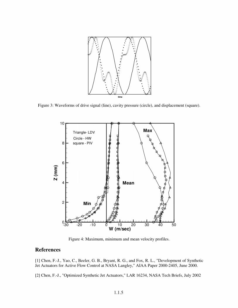
The zero mass jet flow consists of a pulse train of high speed fluids projected form the slot accompanied by a pair of vortices. An elongated mean jet emerges when the flow fields are time or ensemble averaged. The maximum jet velocity (Fig. 4) was found slightly above the slot, and its magnitude may be scaled by the peak cavity pressure, ∝ (pmax)1/2. In the near fields, there was a close comparison found in the velocity profiles obtained by the LDV and PIV, but their magnitudes were off. Good agreements between the LDV and PIV measurements have been reported in liquid experiments, but the discrepancy found in this test has not been resolved. On the other hand, the hot-wire data showed a faster decay of the jet. In the far fields, however, hot-wire and LDV data matched well. Above the maximum jet velocity, the flow is always in upward motion, i.e., its height, about 4 slot width, defines the upper limit of the suction action.

Figure 1: Synthetic jet slot

Figure 2: Synthetic jet performance with frequency.

1.1.4

time

Figure 3: Waveforms of drive signal (line), cavity pressure (circle), and displacement (square).

W (m/sec)

Z(m

m)

-30 -20 -10 0 10 20 30 40 500

2

4

6

8

10

Mean

Max

Min

Triangle- LDV

Circle - HWsquare - PIV

Figure 4: Maximum, minimum and mean velocity profiles.

References [1] Chen, F.-J., Yao, C., Beeler, G. B., Bryant, R. G., and Fox, R. L., "Development of Synthetic Jet Actuators for Active Flow Control at NASA Langley," AIAA Paper 2000-2405, June 2000. [2] Chen, F.-J., "Optimized Synthetic Jet Actuators," LAR 16234, NASA Tech Briefs, July 2002

1.1.5

CASE 1: DETAILS AND SUBMISSION GUIDELINES

Relevant Details

Flow issues into an enclosed box (24 inches on each side) with M_freestream = 0. The atmospheric conditions varied, but were essentially standard atmospheric conditions at sea level, in a temperature-controlled room. These conditions can be given as approximately: p_ambient = approx 101325 kg/(m-s^2) T_ambient inside box = approx 75 deg F (approx 297 K) T inside cavity = approx 83 deg F (approx 301 K). Some derived relevant conditions are: density_ambient = approx 1.185 kg/m^3 viscosity_ambient = approx 18.4e-6 kg/(m-s) The diaphragm frequency = 444.7 Hz. The 2.0 inch-diameter diaphragm is circular, and is held in place with an o-ring seal 1.5 inches in diameter. The displacement (D) at the center of the diaphragm as a function of phase was provided on the web site.

The displacement at the center of the diaphragm is offset - it displaces inward LESS and outward MORE (i.e., the reference position is not zero) Also in the file, the pressure (P) and temperature (T) as a function of phase are given. The location where these quantities are measured are as follows. The pressure is measured inside the cavity on the wall opposite the center of the diaphragm (the pressure is given with respect to an unspecified reference pressure, which may be presumed to be approximately atmospheric). The temperature is measured at the bottom (floor) of the cavity. (The voltage input to the diaphragm, prior to being amplified, is also included in the file, although this is not relevant information for CFD. It has been offset to positive values for LDV purposes.)

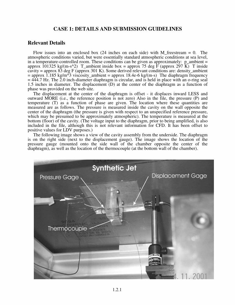
The following image shows a view of the cavity assembly from the underside. The diaphragm is on the right side (next to the displacement gauge). The image shows the location of the pressure gauge (mounted onto the side wall of the chamber opposite the center of the diaphragm), as well as the location of the thermocouple (at the bottom wall of the chamber).

1.2.1

The following figure shows the measured phase-averaged vertical velocity over the center of the slot as a function of phase, using three different measurement techniques. The data files can be found on the web site.

Submission Guidelines

Numerical predictions of this type of statistically unsteady flow are relatively new. The purpose here is to determine the state-of-the-art in modeling these types of unsteady synthetic-jet-type flows, so we want to explore which CFD methods work and which do not. The following options are available

Either model the internal cavity or specify an unsteady boundary condition at the slot exit.

Either model the moving diaphragm, or employ an unsteady boundary condition that approximates its effect within the cavity.

1.2.2

Even though the geometry (and flowfield) is inherently three-dimensional, a two-dimensional model, across the center of the slot, can be used.

It is the requirement that contributors detail specifically how they choose to model the case, including all boundary conditions and approximations made. As the methodologies used are assessed at the workshop, it will be important to know as many details as possible about the calculations/simulations. Detailed requirements include:

1. The case must be run time-accurately, in order to simulate the unsteady nature of the case.

• 1a. RANS codes run in time-accurate mode (e.g., URANS) solve directly for phase-averaged variables, i.e. <ui> and <u'iu'j> (see Appendix for details). Therefore, RANS simulations should result in repeating or very-nearly-repeating periodic solutions. When periodicity is achieved, averages over one or more periods of oscillation yields the long-time-averaged (time-independent mean) values for these quantities.

• 1b. DNS, LES, or DES simulations will need to be post-processed to obtain both the phase-averaged and long-time-averaged (time-independent mean) values.

2. GRID STUDY: If the case is modeled two-dimensionally, then it is strongly suggested that the computation be performed using at least two different grid sizes in order to assess the effect of spatial discretization error on the solution. If it is modeled three-dimensionally, then solutions using more than one grid size are encouraged, but not required. If more than one grid is used, each set of results should be submitted separately.

3. TIME STEP STUDY: If the case is miodeled two-dimensionally, then it is strongly suggested that the computation be performed using at least two different time step sizes in order to assess the effect of temporal discretization error on the solution. If it is modeled three-dimensionally, then solutions using more than one time step are encouraged, but not required. If more than one time step is used, submit each set of results separately.

Specific quantities that result from the computations at particular locations will be required for submission. Note that for all the following, the coordinate system adopted has x across the slot (across the 0.05 inch-wide gap) and y up, with the (x,y)=(0,0) origin at the bottom wall of the "box" into which the jet issues, at the center of the slot opening. All results from 3-D computations are to be given at the z=0 location (across the center of the slot). The requirements follow (if it is not possible to provide a particular quantity, simply leave it out of the "variable" list, and reduce the number of columns of data submitted):

a. Long-time-averaged jet width (width is in the x-direction) as a function of vertical height above the lower wall, from the wall up to a height of at least 20 mm. Define jet width as the horizontal distance between which the vertical velocity exceeds its (maximum+minimum)/2 value (at that vertical height). Name this file: case1.avgjetwidth.ANYTHING.dat-where "ANYTHING" can be any descriptor you choose (should be different for each file if you are submitting multiple runs)-the file should be in 2-column format: 1st line: #your name (pound sign needed) 2nd line: #your affiliation (pound sign needed) 3rd line: #your contact info (pound sign needed) 4th line: #brief description of grid (pound sign needed) 5th line: #number of time steps per cycle (pound sign needed)

1.2.3

6th line: #brief description of code/method (pound sign needed) 7th line: #other info about the case, such as spatial accuracy (pound sign needed) 8th line: #other info about the case, such as turb model (pound sign needed) 9th line: #other info about the case (pound sign needed) 10th line: variables="y, mm","avg jet width, mm" 11th line: zone t="jet width" subsequent lines: y(mm) avgjetw(mm) <- this is the data

The sample file case1.avgjetwidth.SAMPLE.dat can be downloaded from the web site.

1.2.4

b. Long-time-averaged horizontal velocity (u) and vertical velocity (v) profiles along the center of the jet (at the center of the slot), from the wall up to a height of at least 20 mm. Also, submit profiles along nine lines parallel to the wall, at heights of 0.1 mm, 1 mm, 2 mm, 3mm, 4 mm, 5 mm,6 mm, 7 mm, and 8 mm above the lower wall, from at least -10 mm to +10 mm to either side of the jet centerline. Name this file: case1.avgvel.ANYTHING.dat-where "ANYTHING" can be any descriptor you choose (should be different for each file if you are submitting multiple runs) -the file should be in 4-column format: 1st line: #your name (pound sign needed) 2nd line: #your affiliation (pound sign needed) 3rd line: #your contact info (pound sign needed) 4th line: #brief description of grid (pound sign needed) 5th line: #number of time steps per cycle (pound sign needed) 6th line: #brief description of code/method (pound sign needed) 7th line: #other info about the case, such as spatial accuracy (pound sign needed) 8th line: #other info about the case, such as turb model (pound sign needed) 9th line: #other info about the case (pound sign needed) 10th line: variables="x, mm","y, mm","u, m/s","v, m/s" 11th line: zone t="centerline" subsequent lines: x(mm) y(mm) u(m/s) v(m/s) <- this is the data along x=centerline next line: zone t="y=0.1 mm" subsequent lines: x(mm) y(mm) u(m/s) v(m/s) <- this is the data along y=0.1mm next line: zone t="y=1 mm" subsequent lines: x(mm) y(mm) u(m/s) v(m/s) <- this is the data along y=1mm next line: zone t="y=2 mm" subsequent lines: x(mm) y(mm) u(m/s) v(m/s) <- this is the data along y=2mm next line: zone t="y=3 mm" subsequent lines: x(mm) y(mm) u(m/s) v(m/s) <- this is the data along y=3mm next line: zone t="y=4 mm" subsequent lines: x(mm) y(mm) u(m/s) v(m/s) <- this is the data along y=4mm next line: zone t="y=5 mm" subsequent lines: x(mm) y(mm) u(m/s) v(m/s) <- this is the data along y=5mm next line: zone t="y=6 mm" subsequent lines: x(mm) y(mm) u(m/s) v(m/s) <- this is the data along y=6mm next line: zone t="y=7 mm" subsequent lines: x(mm) y(mm) u(m/s) v(m/s) <- this is the data along y=7mm next line: zone t="y=8 mm" subsequent lines: x(mm) y(mm) u(m/s) v(m/s) <- this is the data along y=8mm

The sample data file case1.avgvel.SAMPLE.dat can be downloaded from the website.

c. Phase-averaged quantities at 8 different phases during the cycle: 0 deg, 45 deg, 90 deg, 135 deg, 180 deg, 225 deg, 270 deg, 315 deg.; where you should align the phases of your computation as described below. Submit the following phase-averaged <> quantities: u (m/s), v (m/s), u'u'bar (m^2/s^2), v'v'bar (m^2/s^2), and u'v'bar (m^2/s^2), where u = phase-averaged horizontal velocity component (parallel to lower wall, across the slot), v = phase-averaged vertical velocity component (up, away from lower wall) u'u'bar = phase-averaged turbulent normal stress in horizontal direction (optional) v'v'bar = phase-averaged turbulent normal stress in vertical direction (optional) u'v'bar = phase-averaged turbulent shear stress in x-y plan The

1.2.5

locations for these data are the same as for the long-time-averagedquantities. Name these files: case1.phase000.ANYTHING.dat case1.phase045.ANYTHING.dat case1.phase090.ANYTHING.dat case1.phase135.ANYTHING.dat case1.phase180.ANYTHING.dat case1.phase225.ANYTHING.dat case1.phase270.ANYTHING.dat case1.phase315.ANYTHING.dat -where "ANYTHING" can be any descriptor you choose (should be different for each file if you are submitting multipleruns) -the file should be in 7-column format: 1st line: #your name (pound sign needed) 2nd line: #your affiliation (pound sign needed) 3rd line: #your contact info (pound sign needed) 4th line: #brief description of grid (pound sign needed) 5th line: #number of time steps per cycle (pound sign needed) 6th line: #brief description of code/method (pound sign needed) 7th line: #other info about the case, such as spatial accuracy (pound sign needed) 8th line: #other info about the case, such as turb model (pound sign needed) 9th line: #other info about the case (pound sign needed)

10th line: variables="x, mm","y, mm","u, m/s","v, m/s", "uu, m^2/s^2","vv, m^2/s^2","uv,m^2/s^2"

11th line: zone t="centerline" subsequent lines: x(mm) y(mm) u(m/s) v(m/s) uu(m^2/s^2) vv(m^2/s^2) uv(m^2/s^2) <- this is the data along x=centerline next line: zone t="y=0.1 mm" subsequent lines: x(mm) y(mm) u(m/s) v(m/s) uu(m^2/s^2) vv(m^2/s^2) uv(m^2/s^2) <- this is the data along y=0.1mm next line: zone t="y=1 mm" subsequent lines: x(mm) y(mm) u(m/s) v(m/s) uu(m^2/s^2) vv(m^2/s^2) uv(m^2/s^2) <- this is the data along y=1mm next line: zone t="y=2 mm" subsequent lines: x(mm) y(mm) u(m/s) v(m/s) uu(m^2/s^2) vv(m^2/s^2) uv(m^2/s^2) <- this is the data along y=2mm next line: zone t="y=3 mm" subsequent lines: x(mm) y(mm) u(m/s) v(m/s) uu(m^2/s^2) vv(m^2/s^2) uv(m^2/s^2) <- this is the data along y=3mm next line: zone t="y=4 mm" subsequent lines: x(mm) y(mm) u(m/s) v(m/s) uu(m^2/s^2) vv(m^2/s^2) uv(m^2/s^2) <- this is the data along y=4mm next line: zone t="y=5 mm" subsequent lines: x(mm) y(mm) u(m/s) v(m/s) uu(m^2/s^2) vv(m^2/s^2) uv(m^2/s^2) <- this is the data along y=5mm next line: zone t="y=6 mm" subsequent lines: x(mm) y(mm) u(m/s) v(m/s) uu(m^2/s^2) vv(m^2/s^2) uv(m^2/s^2) <- this is the data along y=6mm next line: zone t="y=7 mm"

1.2.6

subsequent lines: x(mm) y(mm) u(m/s) v(m/s) uu(m^2/s^2) vv(m^2/s^2) uv(m^2/s^2) <- this is the data along y=7mm next line: zone t="y=8 mm" subsequent lines: x(mm) y(mm) u(m/s) v(m/s) uu(m^2/s^2) vv(m^2/s^2) uv(m^2/s^2) <- this is the data along y=8mm

The sample datafile case1.phase000.SAMPLE.dat can be downloaded from the website.

d. Phase-averaged time-history values of <u> and <v> as a function of phase (deg) at three approximate point locations: (x,y)=(0mm,0.1mm), (0mm,2mm), and (1mm,2mm). Give the data at every time step taken. In other words, if your time step yields 100 steps per cycle, then give 100 phases between 0 deg and 360 deg. You should align the phases of your computation as described below. Name this file: case1.phasehist.ANYTHING.dat -where "ANYTHING" can be any descriptor you choose (should be different for each file if submitting multiple runs) -the file should be in 5-column format: 1st line: #your name (pound sign needed) 2nd line: #your affiliation (pound sign needed) 3rd line: #your contact info (pound sign needed) 4th line: #brief description of grid (pound sign needed) 5th line: #number of time steps per cycle (pound sign needed) 6th line: #brief description of code/method (pound sign needed) 7th line: #other info about the case, such as spatial accuracy (pound sign needed) 8th line: #other info about the case, such as turb model (pound sign needed) 9th line: #other info about the case (pound sign needed) 10th line: variables="phase, deg","x, mm","y, mm","u, m/s","v, m/s" 11th line: zone t="x=0 mm, y=0.1 mm"

subsequent lines: phase x(mm) y(mm) u(m/s) v(m/s) <- this is the data at x=0mm, y=0.1mm

next line: zone t="x=0 mm, y=2 mm" subsequent lines: phase x(mm) y(mm) u(m/s) v(m/s) <- this is the data at x=0mm, y=2mm next line: zone t="x=1 mm, y=2 mm" subsequent lines: phase x(mm) y(mm) u(m/s) v(m/s) <- this is the data at x=1mm, y=2mm

The sample datafile case1.phasehist.SAMPLE.dat can be downloaded from the website.

e. Field line-contour-plots (in one of the following formats: ps, eps, or jpg) of phase-averaged <u>-velocity and <v>-velocity at the following phases: 45 deg, 90 deg, 135 deg, and 225 deg.; where you should align the phases of your computation as described below. These plots should be black-and-white line plots only. The plots should go from approx x=-3mm to 3 mm, and y=0mm to y=8mm. The x-to-y ratio of the plot should be 1.0. For all plot files, plot line contours of -20 m/s through 30 m/s in increments of 1 m/s. Either (a) plot the lines of negative velocity as dashed lines and the lines of positive velocity as solid lines, or (b) label the contour lines, or (c) do both. The purpose of submitting these plots is to get a qualitative picture of the phase-averaged flowfield at particular selected times of interest. Altogether, submit 8 plots files. Name these files: case1.phase045.u.ANYTHING.eps case1.phase090.u.ANYTHING.eps case1.phase135.u.ANYTHING.eps case1.phase225.u.ANYTHING.eps case1.phase045.v.ANYTHING.eps

1.2.7

case1.phase090.v.ANYTHING.eps case1.phase135.v.ANYTHING.eps case1.phase225.v.ANYTHING.eps (where the "eps" in this case means encapsulated postscript - use ps, or jpg instead if appropriate).

Definition of Phase for the Computations Matching the same phases with the experiment is not necessarily straightforward. One way to do it is to try to align a quantity from experiment (such as vertical velocity near the jet exit), but this can be imprecise because the CFD and experimental data are not necessarily well-behaved sine-waves. The best criteria for determining phase may in fact be a different measure altogether.

On the other hand, in this workshop a goal is to be able to compare CFD results with each other, so it is important to try to achieve the same phase definitions in order that all computations are similarly aligned. We have tried to choose criteria for determining phase that approximates experiment AND is specific enough so that different CFD solutions can be meaningfully compared.

Therefore, although participants are given some latitude to determine phase as appropriate, we encourage everyone to use the following steps to define phase in a uniform fashion for Case 1:

• Step 1. Output vertical phase-averaged velocity (v) at the following point in space (over the slot) as a function of your iteration or time step number: (x,y,z)=(0, 0.1, 0)mm. Find vmax and vmin over the course of one phase-averaged period.

• Step 2. Compute the mid-value vavg=(vmax+vmin)/2

• Step 3. Define Phase=340 deg as the time when your velocity at this location approximately equals vavg (INCREASING). All other phases can be referenced from this, via the following relation:

Phase=(iter-it340)*360/nstep+340

where:

iter =iteration (or time step) number nstep=no. of time steps per cycle it340=iteration number when Phase=340 according to the above criteria

For example, if the calculation is running at 360 steps per cycle, in order to match the above criteria at time step number 5575, then

Phase=iter-5235

Thus, when iter=5235, then Phase=0; when iter=5415, then Phase=180; when iter=5595, then Phase=360. Note that Phase=360 also corresponds with Phase=0 (it repeats every 360 deg). This is illustrated in the following figure:

1.2.8

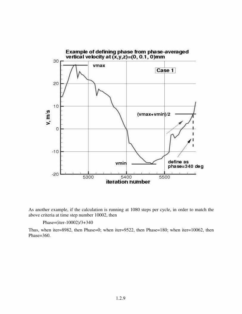
As another example, if the calculation is running at 1080 steps per cycle, in order to match the above criteria at time step number 10002, then

Phase=(iter-10002)/3+340

Thus, when iter=8982, then Phase=0; when iter=9522, then Phase=180; when iter=10062, then Phase=360.

1.2.9

APPENDIX: FLOWS WITH IMPOSED PERIODIC FORCING

Mathematical Background

The flow field is induced by an oscillatory jet of air emanating from a solid boundary. This oscil-latory motion introduces a wave pattern that can be used as a timer for selective sampling of theflow field fluctuations. Thus, the weak organized wave motion can be extracted from a backgroundfield of finite turbulent fluctuations. The mathematical framework outlined here follows closely thatoriginally presented by Hussain and Reynolds (1970, 1972). Some previous work in this area thatmay also be of interest are reported in Gatski and Liu (1980) and Obi, Ishibashi and Masuda (1997).

If such traveling waves exist within the fluctuating flow field, any fluctuating quantity���������

can be decomposed into ����� ���������������������� ������������� ������(1)

where�������

is the (time) mean value,�����������

is the statistical contribution of the organized motion,and

����� ������the turbulence. Since the flow is not stationary, the ergodic hypothesis does not hold

and the ensemble mean does not equal the long time average. Thus, a time average is defined as����!���� "$# %&�')( *+ , &- ����� �����.��(2)

and a phase average is defined as/ ����� ���10 � "$# %23')( *4 25687 - ���������9��:�;�(3)

where;

is the period of the imposed oscillatory motion. The phase average is the average at anypoint in space of the values of

�that are realized at a particular phase < in the cycle of the oscillating

jet. The wave component is then given by������ ������ / ����� ���10�=>�������?�(4)

so that ����� ��@A�� / �B��� ��@A0��C� � ��� ��@A9�(5)

These results show that at any point in the flow a time varying function���������

can be partitionedinto the three components parts defined in Eqs. (2), (3), and (4) given a reference oscillating signalat a given frequency (period). The following properties are associated with the triple-decompositionand prove useful in extracting information about both the mean field(s) and the statistical correla-tions of the fluctuation field. These relations include��EDF�G�� �D�� HI��ED�J��K�� / DE0�� LM��EDONP���� / D909� / ��0��QL���RNS�T��U���V�XWE� � � �YW�� / � � 0��XW�� ��ED � � H ��ED � J �XWBZ (6)

These relations show that the fluctuation� �

is centered about both the time average and phaseaveraged means and that the background turbulence is uncorrelated with the organized motion.

1.2.10

Phase-Averaged Navier-Stokes Equations

In general, both pressure-velocity and density-velocity numerical solvers are used in RANS CFDcodes. In this section, the phase-averaged formulations for both the incompressible and compress-ible forms of the Navier-Stokes equations will be presented. For contributors using time-accurateRANS-type formulations, the dependent variables calculated are the phase-averaged variables de-fined above and shown below to satisfy transport equations that are formaly equivalent to the usualRANS equations.

Incompressible Phase-Averaged Equations

With the decomposition and mathematical framework outlined in Section , it is possible to developa set of phase-averaged Navier-Stokes equations that describe the behavior of the phase-averagedmean quantities as well as the corresponding equations for the phase-averaged turbulent quantities(Gatski and Liu, 1980).

In Section , the phase-averaged mean equations are presented and in Section the phase-averagedturbulent quantities are presented.

Phase-averaged mean equations

The mean flow equations are given by [I\�]�^`_[�aE^cbXd (7a)e \�]�^`_e�f b [I\�]�^`_[ f g \�]ihj_ [B\`]�^`_[�akh bQlnm op [B\rq�_[�a�^ gts [vu�\`]�^�_[�a uh l [Bw�]�x^ ]�xh8y[Oaih z (7b)

From these results, it is possible to obtain the time-independent mean values, for exampleo]�^ b \`]�^`_|{ ]Ex^ ]Exh b wE]�x^ ]�xh y(8)

Phase-averaged turbulent equations

As an example, the phase-averaged formulation for a two-equation\`}~_

-\���_

model will be given.Other models under consideration can be formulated in terms of phase-averaged variables in a sim-ilar fashion.

The transport equations for the phase-averaged turbulent kinetic energy\�}�_�� b \�]Rx^ ]�x^ _9�����

anddissipation rate

\���_are given bye \�}�_e?f bQ� ] x^ ] x �8� [�\�]E^!_[�a � l \���_ g [[�a ���8� s)g s���E�n� [I\`}~_[�a ��� (9)e \���_e?f bQlP����� \���_\�}�_P� ] x^ ] x ��� [�\�]�^`_[�a � l���� u \!��_ u\`}�_ g [[�a � �8� s�g s��� � � [�\���_[�a � � (10)

where ��� , � � , ����� , and ��� u are closure coefficients, and an eddy viscosity relationship is assumedfor the individual phase-averaged stress components so that� ] x^ ] xh � b �� \�}�_���^�h l s�� � [�\�]�^`_[�a h g [�\�]khj_[�a ^ � {

(11a)

with s�� b��S  \`}�_ u\���_ (11b)

and �S  a closure coefficient.

1.2.11

Compressible Phase-Averaged Equations

In a compressible formulation, where Favre averaged variables are used, that is ¡�¢k£!¤R¥¡ , the definitionof the phase average has to be altered. In this case the compressible phase-averaged variables aredefined as ¦ ¢E£!§�¨ ¦ ¡i¢E£!§¦ ¡i§ª© (12)

and the flow variables are partitioned as in Eq. (5). In Section , the phase-averaged mean equationsare presented and in Section the phase-averaged turbulent quantities are presented.

Phase-averaged mean equations

In terms of phase-averaged Favre variables, the mass conservation equation can be written as« ¦ ¡�§«�¬­¨¯® ¦ ¡i§® ¬±° ¦ ¢i²j§�® ¦ ¡i§®�³ ² ¨µ´ ¦ ¡�§�® ¦ ¢ ² §®�³ ² © (13a)

and the conservation of momentum as¦ ¡i§ « ¦ ¢ £ §«?¬ ¨Q´�® ¦ ¶ §®O³ £ °·® ¦�¸ £�² §®�³ ² ´ ® ¦ ¡i§�¹E¢�º£ ¢�º²¼»®�³ ² ½ (13b)

where ¦�¸ £�²j§�¨X¾ ¿ÁÀ¼Â¾�à ® ¦ ¢�£`§®�³ ² °Q® ¦ ¢k²j§®�³ £~Ä ´QÂÅ ® ¦ ¢9Æ�§®O³ ÆXÇ £�²�È ½ (13c)

A phase-averaged conservation of total energy equation can be written as®�É ¦ ¡�§ ¦!Ê §1Ë® ¬ ° ®�É ¦ ¢k²A§ ¦ ¡�§ ¦�Ì §1Ë®O³ ² ¨ ® ¦ ¢E£Í¡ Ê §®�³ ² ´ ® ¦`Î ²A§®�³ ² © (14)

where the total energy and total enthalpy,

¦ ¡�§ ¦�Ê § and

¦ ¡�§ ¦!Ì § , respectively, are¦�Ê §Ï¨ Ð�Ñ ¦�Ò §�° ¦ ¢E£!§ ¦ ¢�£`§¾ ° ¦ ¢�º£ ¢�º£ §¾ © (15a)¦`Ì §�¨ ¦�Ê §�° ¦ ¶ §¦ ¡i§ © (15b)

and ¦`Î ² §�¨Q´ÔÓ�Õ�Ö ® Ò®�³ ²�×ÙØ ´ ÕkÖ ® ¦ÍÒ §®�³ ² © (16a)¦ ¢ ² ¡ Ê §U¨XÐ�Ú ¦ ¡�§�ÛÜ¢ º² Ò º�Ý ° ¦ ¢ £ §�Þ ¦ ¡�§�Ûj¢ º£ ¢ º² Ý ´ ¦�¸ £�² §�ß ° ¦ ¡�§ ¹ ¢Eº£ ¢�º£ ¢�º² »¾ ´tÛ|¢ º£ ¸ º£�² Ý ½ (16b)

From these results, it is possible to obtain the time-independent mean values, for example¥¡�¨ ¦ ¡i§ © ¥¢ £ ¨ ¦ ¢ £ § © ¥Ê ¨ ¦�Ê § © ¥Î £ ¨ ¦`Î £ § © ¢ º£ ¢ º² ¨ ¹ ¢ º£ ¢ º² » (17)

1.2.12

Phase-averaged turbulent equations

Once again, a phase-averaged formulation for a two-equation à`á~â - à�ã�â model is used. Other modelscan be formulated in terms of phase-averaged Favre variables in a similar fashion.

The transport equations for the phase-averaged turbulent kinetic energy à�á�â�äæåQà�çRèé`ç�èé`â9ê�ë�ì anddissipation rate à�ã�â are given byàæíiâ�î à�á�âî�ï åQà`í�â9ð|ç èé ç è ñ�ò�ó à`ç é âóOô ñöõ à�íiâ�à�ã�â�÷ óó�ô ñ�ø¼ùEú ÷ ú�ûü�ýÿþ ó à�á�âó�ô ñ�� (18)

à�í�â�î à ã�âî?ï å õ������ à`í�â à ã�âà�á�â ð ç èé ç è ñ ò ó à�ç é âóOô ñ õ���� à�í�â à�ã�â à�á�â ÷ óó�ô ñ�ø8ù ú ÷ ú ûü � þ ó à�ã�âó�ô ñ�� (19)

where ü�ý , ü � , ����� , and � � are closure coefficients, and an eddy viscosity relationship is assumedfor the individual phase-averaged stress components so thatà`í�â�ðÜç èé ç è� ò å ë� à`í�â9à�á~â�� é � õ�ú û ù ó à`ç é âó�ô � ÷ ó à�ç � âóOô é þ�� (20a)

with ú û å ��� àæíiâ à�á�â à�ã�â (20b)

and ��� a closure coefficient.

References

Gatski, T. B. and Liu, J. T. C. 1980 On the interaction between large-scale structure and fine-grained turbulence in a free shear flow. III. A numerical solution Phil. Trans. Roy. Soc. London293, 473-509.

Hussain, A. K. M. F. and Reynolds, W. C. 1970 The mechanics of an organized wave in turbulentshear flow. J. Fluid Mech. 41, 241-258.

Hussain, A. K. M. F. and Reynolds, W. C. 1972 The mechanics of an organized wave in turbulentshear flow. Part 3. Theoretical models and comparisons with experiments J. Fluid Mech. 54,263-288.

Obi, S., Ishibashi, N., and Masuda, S. 1997 The mechanism of momentum transfer enhancementin the periodically perturbed turbulent separated flow 2nd Int. Symposium on Turbulence, Heat andMass Transfer (K. Hanjalic and T. W. J. Peeters, Eds.), Delft University Press, 835-844.

1.2.13

CASE 1: NUMERICAL SIMULATION OF A SYNTHETIC JET INTOA QUIESCENT AIR

I. Mary1

1 CFD and Aeroacoustic Departement, ONERA Chatillon, France

Introduction

Three different simulations of the case 1 have been carried out in order to assess the influence of the tur-bulence modelling. Firstly two-dimensional URANS and laminar simulations have been first investigated.As the Reynolds number based on cavity charateristics (like the diaphragm velocity and the exit size of thecavity) is quite small (less than 10000), it is not obvious that an URANS simulation will be better adaptedto this flow case than a laminar simulation. Moreover the discontinuities in the geometry of the cavity couldcreate complex flow patterns inside the cavity despite the low value of the Reynolds number. Thus three-dimensional Large Eddy Simulation have been realized for the same two-dimensional geometry in order toevaluate the intensity of the three-dimensional effects inside the cavity.

Solution Methodology

General description

The solver FLU3M, developed by ONERA, is based on a cell-centered finite volume technique and struc-tured multi-block meshes. The viscous fluxes are discretized by a second-order accurate centered scheme.For efficiency reason, an implicit time integration is employed to deal with the very small grid size en-countered near the wall. Then a three-level backward differentiation formula is used to approximate thetemporal derivative associated with the unsteady Navier-Stokes equations, leading to second-order accu-racy. An approximate Newton method is employed to solve the non-linear problem. At each iteration of thisinner process, the inversion of the linear system relies on Lower-Upper Symmetric Gauss-Seidel (LU-SGS)implicit method. More details about these numerical points are available in Ref.[1].

Euler fluxes discretization

Usually LES requires a high-order centered scheme for the Euler fluxes discretization (with spectral-likeresolution) in order to minimize dispersive and dissipative numerical errors. However such scheme cannotbe applied easily in complex geometry. Indeed, most of aerodynamic codes able to deal with such a geometryare based on finite-volume technique in order to handle degenerated cell. Thus getting a high-order methodbecomes very time consuming due to the high-order quadrature needed to compute the fluxes along the cellboundaries. As several works (see Ref.[2] for instance) have shown that LES can be carried out with low-order centered scheme in case of sufficient mesh resolution, only second-order accurate scheme is employedin this study. But a special effort has been carried out to minimize the intrinsic dissipation of the schemeand its computational cost.

The AUSM+(P) [3, 4] scheme, whose dissipation is proportional to the local fluid velocity, constitutesthe basis of the discretization, because it is well adapted to low Mach number boundary layer simulations.However several modifications have been introduced to enhance its accuracy and computational cost. As weare not interested by the shock capturing properties of the scheme, simplified formula are developed for this

1.3.1

study to approximate the Euler fluxes:

Fi+1/21 = U1(QL +QR)/2 − |Udis|(QR −QL)/2 + P (1)

where U1 denotes the interface fluid velocity, L/R the left and right third-order MUSCL interpolation.The state vector Q is defined as (ρ, ρu1, ρu2, ρu3, ρE + p)t, whereas the pressure term P is given by(0, (pL+ pR)/2, 0, 0, 0). The symbol Udis, which indicates a local fluid velocity, characterizes the numericaldissipation acting on the velocity components. To enforce the pressure/velocity coupling in low Machnumber zone, a pressure stabilization term is added to the interface fluid velocity as done by Rhie and Chow[6] for incompressible flow:

U1 = (u1 L + u1 R)/2 − c2(pR − pL) (2)

where c2 is a constant parameter. The parameter Udis is defined as follow:

Udis = Φ max (|u1 L + u1 R|/2, c1) (3)

where c1 is a constant parameter and Φ a sensor used to minimize the numerical dissipation. For an accuracyreason, the values of c1 and c2 should be chosen as small as possible to minimize the numerical dissipation.For a stability reason, these parameters cannot be smaller than the threshold value 0.04, which has beendetermined in [5].The present sensor Φ is a binary function, which only depends on the smoothness of theprimitive variables ψ = (ρ, u1, u2, u3, p)

t. If no spurious oscillation is detected on ψ at cell i, Φ is equalto 0. Otherwise Φ is set to 1 at i + 1/2 and i − 1/2 interfaces. To detect a spurious oscillation and defineexactly the sensor used in Eq.(3), the following functions are introduced:

∆iφ =

{−1 if (φi+2 − φi+1)(φi+1 − φi) < 0

1 else

Wψk=

{1 if ∆i

ψk+ ∆i+1

ψk< 0 or ∆i

ψk+∆i−1

ψk< 0

0 elseΦ = max(Wψk

) for k=1,5

(4)

For the two-dimensional laminar and URANS simulations, there is no need to capture the small scaleseddies. Therefore for these simulations the value of Φ is fixed to 1, and the scheme is then purely upwind.

Model Description

Three different kinds of turbulence modelling have been used to compute the test case 1 in order to as-sess their influence for such flow. First a laminar two-dimensional computation has been carried out. Atwo-dimensional URANS simulation has been performed as well, based on the classical Spalart-Allmarasmodel. Finally a three-dimensional LES simulation has been computed. This simulation is based on an eddyviscosity model developed at ONERA: the selective mixed scale model.

Selective mixed scale model

Due to the large computational cost of the intended simulation, only one explicit subgrid scale model hasbeen used for this study. The selective mixed scale model, developed by Sagaut and Lenormand, has beenretained, because a good compromise between accuracy, stability and computational cost is obtained [7].More particularly, the use of a selective function allows to handle transitional flows [8], which is one of thekeypoint of the present application. The eddy viscosity is given using a non-linear combination of the filteredshear stress tensor, a characteristic length scale, the small scale kinetic energy, and a selective function:

µt = ρfθ0(θ)Cm∆3/2√

0.5Sij(u)Sij(u)√Kc (5)

1.3.2

x (m)

y(m

)

-0.02 0 0.02

-0.04

-0.02

0

132

224

134

80

Figure 1: Diaphragm and grid representation

where the test field kinetic energy is evaluated as Kc =√

0.5(ui)′(ui)

′ . The test field (ui)′

is extracted

from the resolved field, (ui)′

= ui − ui, by employing a three-dimensional averaging test filter denoted byui = Ai(Aj(Ak(ui))), with the following definition of Al:

Al(φ) = 0.25φl−1 + 0.5φl + 0.25φl+1 (6)

The characteristic length scale, ∆, is given by the cube root of the cell volume of the mesh, and the constantparameter, Cm = 0.06, is derived in Ref.[9] from isotropic homogeneous turbulence flow cases. Theselective function is defined by:

fθ0(θ) =

{1 if θ > θ0 = 10o

tan4(θ2)/tan4(θ0

2) otherwise (7)

where θ is the angle between the filtered vorticity, ω(u) and the local averaged filtered vorticity, ω(u).

Implementation and Case Specific Details

Diaphragm modelling

A two-dimensional geometry of the case 1 has been retained for this study (see the Fig. 1). No motion isapplied to the mesh at the interface of the diaphragm. Therefore the velocity is imposed at the boundaryof the computational domain by using a time derivative of the time history of the diaphragm displacementgiven in the workshop experimental data.

V (y) = 0.5sin(2 × π × 444.7 × t) ∀y (8)

The use of this unsteady boundary condition generates vortices inside the cavity, which are illustrated on theFig. 2.

Concerning the thermodynamic variables, the density and the pressure are obtained at the wall thanks toa zero order extrapolation.

1.3.3

a) x(m)

y(m

)

-0.01 0 0.01

-0.021

-0.014

-0.007

0

b) x(m)

y(m

)

-0.01 0 0.01

-0.021

-0.014

-0.007

0

c) x(m)

y(m

)

-0.01 0 0.01

-0.021

-0.014

-0.007

0

d) x(m)

y(m

)

-0.01 0 0.01

-0.021

-0.014

-0.007

0

Figure 2: Illustration of the flow structures near the diaphragm: a) t=T/4. b) t=T/2. c) t=T/3. d) t=T.

Time integration

The time step of all the simulations is fixed at ∆t = 0.4497414µs (5000 time steps per period of thediaphragm motion). The number of iteration in the Newton process is equal to 4, which is sufficient for thiscase to deacrease the residual of the non-linear equations by about one order of magnitude.

Grids

A multi-block mesh has been generated for this study. The size of the two-dimensional computationaldomain is identical to those provided on the web-site of the workshop. However the cell distribution differssignificantly. At the cavity exit, the grid spacing is equal to 0.1 mm in the y direction. In the exit channelof the cavity, there are 80 cells in the x direction. The grid spacing at the wall is equal to ∆x = 0.004mm. Therefore there are around 30 cells located in the boundary layer. In the streamwise direction, thereis 134 cells distributed in the upper part of the channel (see Fig. 1). For the external flow there are 217 and131 cells distributed in the x and y direction, respectively. A refinement has been used near the cavity exit.Therefore in the y direction, 80 cells are located between y=0 and y=20 mm, whereas in the x direction themesh has been adapted to the tickening of the jet. Therefore 100 cells are located inside the jet diameterindependantly of the y location. For the three-dimensional LES simulation, the same grid has been used inthe (x,y) plan. In the z direction, the spanwise extent of the computational domain is equal to Lz = 1.3mm,which is almost the size of the jet diameter at the cavit exit. In the spanwise direction 20 cells are uniformelydistributed.

Non-reflective boundary conditions are used in the farfield. At the wall, a no-slip adiabatic condition

1.3.4

has been retained. For the three-dimensionnal LES simulation, the same boundary conditions are used.Moreover flow periodicity is assumed in the spanwise direction.

References

[1] M. Pechier, Ph. Guillen and R. Gayzac, “Magnus Effect over Finned Projectiles,” J. of Spacecraft andRockets, Vol. 38, No 4, pp. 542–549, 2001.

[2] X. Wu, R. Jacobs, J. Hunt and P. Durbin, “Simulation of Boundary Layer Transition Induced by Peri-odically Passing Wake,” J. Fluid Mech., Vol 398, pp. 109–153, 1999.

[3] J. R. Edwards and M. S. Liou, “Low-Diffusion Flux-Splitting Methods for Flows at All Speeds,” AIAAJ., Vol 36, No 9, pp. 1610–1617, 1998.

[4] I. Mary, P. Sagaut and M. Deville, “An algorithm for unsteady viscous flows at all speeds,” Int. J.Numer. Meth. Fluids, Vol 34, No 5, pp. 371–401, 2000.

[5] I. Mary, “Methode de Newton approchee pour le calcul d’ecoulements instationnaires comportant deszones a tres faibles nombres de Mach”,PhD thesis, Univ. Parix XI, Mechanical Dept., october 1999.

[6] C. M. Rhie and W. L. Chow, “Numerical Study of the Turbulent Flow Past an Airfoil with TrailingEdge Separation,” AIAA J., Vol 21, No 11, pp. 1525–1532, 1983.

[7] E. Lenormand, P. Sagaut, L. Ta Phuoc and P. Comte, “Subgrid-Scale Models for Large-Eddy Simula-tion of Compressible Wall Bounded Flows,” AIAA J., Vol 38, No 8, pp. 1340–1350, 2000.

[8] E. David, “Modelisation des ecoulements compressibles et hypersoniques: une approche instation-naire” PhD thesis, Inst. National Polytechnique de Grenoble, Mechanical Dept., october 1999.

[9] P. Sagaut, “Large-eddy simulation of incompressible flows. An introduction.”, pp 101, Springer-Verlag,Berlin, 2001.

[10] P. Spalart and S. Allmaras, “A one-equation turbulence model for aerodynamic flows,” La RechercheAerospatiale, pp 5–21, 1994.

1.3.5

CASE 1: SIMULATION OF A SYNTHETIC JET IN QUIESCENT AIRUSING TLNS3D FLOW CODE

Veer N. Vatsa � and Eli Turkel �� Computational Modeling & Simulation Branch, NASA Langley Research Center, Hampton, VA� Tel Aviv University, Israel & NIA, Hampton, VA

Governing Equations and Solution Methodology

In the present work, a generalized form of the thin-layer Navier-Stokes equations is used to model theturbulent, viscous flow encountered in a synthetic jet. The equation set is obtained from the complete Navier-Stokes equations by retaining the viscous diffusion terms normal to the solid surfaces in every coordinatedirection. For a body-fitted coordinate system ���������� "! fixed in time, these equations can be written in theconservative form as:#%$ �'&(!$�) * $ �'+-,.+�/�!$ � * $ �102,304/�!$ � * $ �'52,356/�!$ 798 (1)

where & represents the conserved variable vector. The vectors + , 0 , 5 , and + / , 0 / , 5 / represent theconvective and diffusive fluxes in the three transformed coordinate directions, respectively. In Eqn. (1), Jrepresents the cell-volume or the Jacobian of coordinate transformation. A multigrid based, general purposemulti-block structured grid approach is used for the solution of the governing equations. In particular,the TLNS3D flow code is used in this study to solve Eqn. (1). Several references exist describing thediscretization and algorithmic details of TLNS3D code. We include only a brief summary of the generalfeatures, and refer to the work of Vatsa and co-workers [1, 2] for further details regarding the TLNS3D code.

Numerical Discretization

The spatial terms in Eqn. (1) are discretized using a standard cell-centered finite-volume scheme. The con-vection terms are discretized using second-order central differences with scalar/matrix artificial dissipation(second- and fourth- difference dissipation) added to suppress the odd-even decoupling and oscillations inthe vicinity of shock waves and stagnation points [3, 4]. The viscous terms are discretized with second-orderaccurate central difference formulas [1]. For the present computations, the Spalart-Allmaras (SA) model [5]and the Menter’s SST model [6] are used for simulating turbulent flows.

For temporal discretization, the convective and diffusive terms are grouped together, and Eqn. (1) canbe rewritten as: : &: ) 7 ,�;6�'&6! *=<?> �'&6! *-<A@ �'&6! (2)

where ;B�'&6! , <C> �'&6! , and<D@ �'&6! are the convection, physical diffusion, and artificial diffusion terms,

respectively. The cell-volume or the Jacobian of coordinate transformation being included in these terms.The time-derivative term can be approximated to any desired order of accuracy by the Taylor series: &: ) 7 EF )�GIHKJ &(LNM � * H � &(L * H � &(LPO � * HPQ &(LKO � *SRTR�R U (3)

1.4.1

Eqn. (3) represents a generalized backward difference scheme (BDF) in time, where the order of accuracy isdetermined by the choice of coefficients VPW , V�X , V"Y ... etc. For example, if VZW%[]\K^I_ , V`X [ba c and VdY []^I_ ,it results in a second-order accurate scheme (BDF2) in time, which is the primary scheme chosen for thiswork due to its robustness and stability properties [7].

In Eqn. (3), the superscript n represents the time level at which the solution is known, and n+1 refersto the next time level to which the solution will be advanced. Similarly, n-1 refers to the solution at onetime level before the current solution. Regrouping the time-dependent terms and the original steady-stateoperator leads to the equation: V Wegfih(jlk Xnmpo6q h jPr jKs X rutut vewf [yx q h(j v (4)

where o6q h jPr jPs X rututIv depends only at solution vector at time levels n and prior, and S represents the steadystate operator or the right hand side of Eqn.(2). By adding a pseudo-time term, we can rewrite the aboveequation as: z hz�{ m V Wegf h jNk X m o6q h jKr jPs X rututIvegf [Sx q h j v (5)

Solution Algorithm

The algorithm used here for solving unsteady flows relies heavily on the steady-state algorithm availablein the TLNS3D code [1]. The basic algorithm consists of a five-stage Runge-Kutta time-stepping schemefor advancing the solution in pseudo-time, until the solution converges to a steady-state. Efficiency of thisalgorithm is enhanced through the use of local time-stepping, residual smoothing and multigrid techniquesdeveloped for solving steady-state equations. In order to solve the time-dependent Navier-Stokes equations(Eqn. 5), we added another iteration loop in physical time outside the pseudo-time iteration loop in TLNS3D.For fixed values of x q h j v , o6q h jPr jKs X rutut v , we iterate on h jNk X using the standard multigrid procedure ofTLNS3D developed for steady-state, until desired level of convergence is achieved. This strategy, originallyproposed by Jameson [8] for Euler equations and adapted for the TLNS3D viscous flow solver by Melsonet. al [7] is popularly known as the dual time-stepping scheme for solving unsteady flows. The process isrepeated until the desired number of time-steps have been completed. The details of the TLNS3D flow codefor solving unsteady flows are available in Refs. [7] and [9].

Boundary Conditions

Except for the moving diaphragm, standard boundary conditions, such as the no-slip, no injection, fixedwall temperature or adiabatic wall, far-field and extrapolation conditions are used as appropriate for thevarious boundaries. The most accurate procedure to simulate the moving diaphragm would require movinggrid capability. For simplicity, we chose to simulate this type of boundary condition by a periodic tran-spiration velocity condition. The frequency of the transpiration velocity at the diaphragm surface in thenumerical simulation corresponded to the frequency of the oscillating diaphragm, and the peak velocity atthe diaphragm surface was obtained from numerical iteration so as to match the experimentally measuredpeak velocity of the synthetic jet emanating from the slot exit. The pressure at the moving diaphragm is alsorequired for closure. However, in the absence of unsteady pressure data from the experiment, we imposeda zero pressure gradient at the diaphragm boundary. We also tested the pressure gradient boundary condi-tion obtained from one-dimensional normal momentum equation [10], which had very little impact on thesolutions. Due to the simplicity and robustness, we selected the zero pressure gradient boundary conditionat the diaphragm surface.

1.4.2

Implementation and Case Specific Details

Although the actuator geometry is highly three-dimensional, the outer flow field is nominally two-dimensionalbecause of the high aspect ratio of the rectangular slot. For the present study, this configuration is modeledas a two-dimensional problem. A multi-block structured grid available at the CFDVAL2004 website is usedas a baseline grid.

The periodic motion of the diaphragm is simulated by specifying a sinusoidal velocity at the diaphragmsurface with a frequency of 450 Hz., corresponding to the experimental setup. The amplitude is chosen sothat the maximum Mach number at the jet exit is approximately |~}T� , to replicate the experimental conditions.At the solid walls zero slip, zero injection, adiabatic temperature and zero pressure gradient conditions areimposed. In the external region, symmetry conditions are imposed on the side (vertical) boundaries andfar-field conditions are imposed on the top boundary. A nominal free-stream Mach number of 0.001 isimposed in the free stream to simulate incompressible flow conditions in the TLNS3D code, which solvescompressible flow equations.

The code was run in unsteady (URANS) mode until the periodicity was established. The time-meanquantities were obtained by running the code for at least another 15 periods and averaging the flow quantitiesover these periods. The phase-locked average of flow quantities were assumed to be coincident with theirvalues during the last full time period.

Results/Discussion

Only a brief set of results is included here, detailed results will be available in the workshop proceedings.Majority of the solutions were obtained with SA turbulence model on the baseline grid with a time-step of�g�D�����Z�'��T����P�K�

, where�~�Z�'��T��

represents the physical time for a complete period. In addition, resultswere generated for the following conditions: (a) coarser grid (cg) obtained by eliminating every other pointfrom the baseline grid; (b) finer grid (fg) generated by increasing resolution in the normal direction by �K|P� ;(c) lower time-step (lower dt), where

�g�(��� �Z������� � �Z�P� ; and (d) Menter’s SST turbulence model. Theresults for the vertical velocity near the slot exit center line (x=0., y=0.1 mm) from these computations arecompared in Fig. 1, which shows very little sensitivity to turbulence model change, and spatial and temporalresolutions.

Next we show the results for time-averaged velocity along the jet center line in Fig. 2. In the proximityof the slot exit (y � � mm ), all 5 sets of results are indistinguishable, and are in good agreement with thehotwire data. However, further away from the slot, the coarse grid (cg) results show significant deviationfrom the baseline results. The effect of turbulence model type (SA or SST) are also more pronounced in theouter region. Similar trends are observed in Fig. 3 for the jet width based on time-averaged solutions.

Based on these results and more detailed comparisons (not shown here) of the computational resultsfor time-averaged and phase-locked average velocities, the effect of lowering the time-step and refining thenormal mesh were found to be very small. Noticeable differences were observed for the coarse grid (cg)results in the outer regions. The difference between the SA and SST turbulence model results become morepronounced in regions further away from the slot exit.

References

[1] Vatsa, V.N. and Wedan, B.W.: “Development of a multigrid code for 3-d Navier-Stokes equations andits application to a grid-refinement study”. Computers and Fluids. 18:391-403. 1990.

[2] Vatsa, V.N.; Sanetrik, M.D.; and Parlette, E.B.: “Development of a Flexible and Efficient Multigrid-Based Multiblock Flow Solver”. AIAA paper 93-0677, Jan. 1993.

[3] Turkel, E. and Vatsa, V.N.: “Effect of artificial viscosity on three-dimensional flow solutions”. AIAAJournal, vol. 32, no. 1, Jan. 1994, pp. 39-45.

1.4.3

[4] Jameson, A.; Schmidt, W.; and Turkel, E.: “Numerical Solutions of the Euler Equations by FiniteVolume Methods Using Runge-Kutta Time-Stepping Schemes”. AIAA Paper 1981-1259, June 1981.

[5] Spalart, P.A. and Allmaras, S.R.:“A one-equation turbulence model for aerodynamic flows”. AIAAPaper 92-439, Reno, NV, Jan. 1992.

[6] Menter, F.R.: “Zonal Two Equation k- � Turbulence Models for Aerodynamic Flows”. AIAA paper93-2906, Orlando, Fl, 1993.

[7] Melson,N.D.; Sanetrik, M.D.; and Atkins, H.L.:“Time-accurate calculations with multigrid acceler-ation”. Appeared in “Proceedings of the Sixth Copper Mountain conference on multigrid methods”,1993, edited by: Melson, N.D.; Manteuffel, T.A.; and S.F. McCormick, S.F.

[8] Jameson, A.: “Time Dependent Calculations Using Multigrid, with Applications to Unsteady Flowspast Airfoils and Wings”. AIAA Paper 91-1596, 1991.

[9] Bijl, H.; Carpenter, M.H.; and Vatsa, V.N.: “Time Integration Schemes for the Unsteady Navier-StokesEquations”. AIAA Paper 2001-2612.

[10] Rizzetta, D.P.; Visbal. M.R.; and Stanek, M.J.: “Numerical Investigation of Synthetic Jet Flowfields”.AIAA Paper 98-2910, June 1998.

0 90 180 270 360Phase angle (deg)

−30

−20

−10

0

10

20

30

V−v

el (m

/sec

)

Exp. data, PIVtlns3d−sa (baseline)tlns3d−sa (cg)tlns3d−sa (fg)tlns3d−sa (low dt)tlns3d−sst (baseline)

Figure 1: Time-variation of V-velocity at slot exit, x=0., y=0.1 mm

1.4.4

0 4 8 12 16 20y (mm)

0

2

4

6

8

10

cent

erlin

e V

−vel

ocity

(m/s

ec)

Exp. data, PIVExp. Data, Hotwiretlns3d−sa (baseline)tlns3d−sa (cg)tlns3d−sa (fg)tlns3d−sa (low dt)tlns3d−sst (baseline)

Figure 2: Center-line average velocity comparisons

0 1 2 3 4 5 6 7 8Jet Width (mm)

0

2

4

6

8

10

12

14

16

18

20

Y (m

m)

Exp. Data (PIV)tlns3d−sa (baseline)tlns3d−sa (cg)tlns3d−sa (fg)tlns3d−sa (low dt)tlns3d−sst (baseline)

Figure 3: Jet-width comparisons

1.4.5

CASE 1: SYNTHETIC JET INTO QUIESCENT AIR.URANS SIMULATIONS WITH EDDY-VISCOSITY AND

REYNOLDS-STRESS MODELS

Sabrina Carpy � and Remi Manceau �� Laboratoire d’etudes aerodynamiques, UMR 6609, University of Poitiers/CNRS/ENSMA, France

Introduction

Computations of a synthetic jet (Case 1) are performed with Code Saturne, a finite-volume solver on un-structured grids developed at EDF [1]. The purpose of the present work is to investigate the ability of stan-dard turbulence models (eddy-viscosity and Reynolds-stress models) to close the phase-averaged Navier–Stokes equations. Therefore, this unsteady flow was run with usual RANS-equations solved in time-accuratemode (URANS), using the standard � – � model [4] and the Rotta+IP second moment closure [3, 2]. Wallfunctions were used at all solid boundaries. All the computations are 2-dimensional.

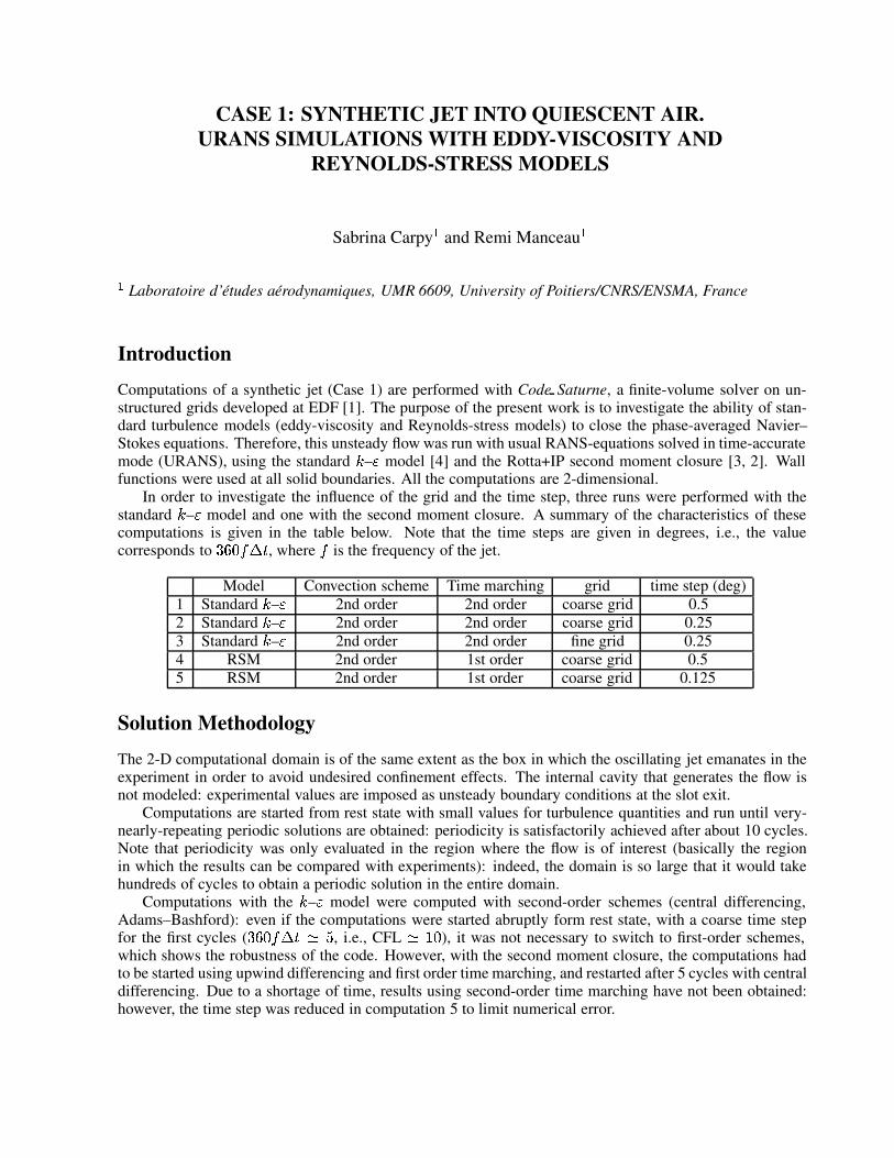
In order to investigate the influence of the grid and the time step, three runs were performed with thestandard � – � model and one with the second moment closure. A summary of the characteristics of thesecomputations is given in the table below. Note that the time steps are given in degrees, i.e., the valuecorresponds to �l�N�P���g� , where � is the frequency of the jet.

Model Convection scheme Time marching grid time step (deg)1 Standard � – � 2nd order 2nd order coarse grid 0.52 Standard � – � 2nd order 2nd order coarse grid 0.253 Standard � – � 2nd order 2nd order fine grid 0.254 RSM 2nd order 1st order coarse grid 0.55 RSM 2nd order 1st order coarse grid 0.125

Solution Methodology

The 2-D computational domain is of the same extent as the box in which the oscillating jet emanates in theexperiment in order to avoid undesired confinement effects. The internal cavity that generates the flow isnot modeled: experimental values are imposed as unsteady boundary conditions at the slot exit.

Computations are started from rest state with small values for turbulence quantities and run until very-nearly-repeating periodic solutions are obtained: periodicity is satisfactorily achieved after about 10 cycles.Note that periodicity was only evaluated in the region where the flow is of interest (basically the regionin which the results can be compared with experiments): indeed, the domain is so large that it would takehundreds of cycles to obtain a periodic solution in the entire domain.

Computations with the � – � model were computed with second-order schemes (central differencing,Adams–Bashford): even if the computations were started abruptly form rest state, with a coarse time stepfor the first cycles ( �l�N�P���g�w ¢¡ , i.e., CFL  ¤£Z� ), it was not necessary to switch to first-order schemes,which shows the robustness of the code. However, with the second moment closure, the computations hadto be started using upwind differencing and first order time marching, and restarted after 5 cycles with centraldifferencing. Due to a shortage of time, results using second-order time marching have not been obtained:however, the time step was reduced in computation 5 to limit numerical error.

1.5.1

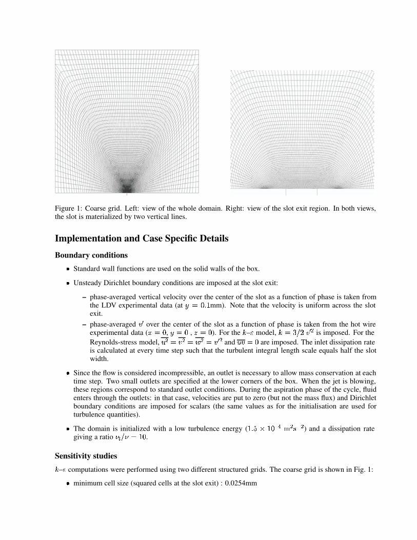
Figure 1: Coarse grid. Left: view of the whole domain. Right: view of the slot exit region. In both views,the slot is materialized by two vertical lines.

Implementation and Case Specific Details

Boundary conditions¥ Standard wall functions are used on the solid walls of the box.¥ Unsteady Dirichlet boundary conditions are imposed at the slot exit:

– phase-averaged vertical velocity over the center of the slot as a function of phase is taken fromthe LDV experimental data (at ¦�§©¨`ªT« mm). Note that the velocity is uniform across the slotexit.

– phase-averaged ¬®­ over the center of the slot as a function of phase is taken from the hot wireexperimental data ( ¯°§y¨ , ¦(§±¨ , ²A§±¨ ). For the ³ – ´ model, ³B§¶µP·N¸¹¬ ­ º is imposed. For theReynolds-stress model, » º § ¬ º § ¼ º §½¬K­uº and »�¬g§¾¨ are imposed. The inlet dissipation rateis calculated at every time step such that the turbulent integral length scale equals half the slotwidth.¥ Since the flow is considered incompressible, an outlet is necessary to allow mass conservation at each

time step. Two small outlets are specified at the lower corners of the box. When the jet is blowing,these regions correspond to standard outlet conditions. During the aspiration phase of the cycle, fluidenters through the outlets: in that case, velocities are put to zero (but not the mass flux) and Dirichletboundary conditions are imposed for scalars (the same values as for the initialisation are used forturbulence quantities).¥ The domain is initialized with a low turbulence energy ( «NªI¿°À=«Z¨Á~ÂÄÃAºZÅ�Á�º ) and a dissipation rategiving a ratio Æ�ÇÈ·NÆ4§É«Z¨ .

Sensitivity studies³ – ´ computations were performed using two different structured grids. The coarse grid is shown in Fig. 1:¥ minimum cell size (squared cells at the slot exit) : 0.0254mm

1.5.2

Ê maximum cell size : 12.5mmÊ number of cells : 15707

For the fine grid, each cell has been divided into four cells, leading to 62828 cells. Some characteristics ofthe flow are sensitive to the grid, such as the width of the jet (long-time averaged flow), but the dynamics isby no means influenced.

As shown in the table above, different time steps were used in order to evaluate the numerical error dueto the time-marching scheme. The results are only marginally influenced by the reduction of the time step.

References

[1] F. Archambeau et al. A finite volume method for the computation of turbulent incompressible flows.Submitted to Int. J. Finite Volumes, 2004.

[2] S. Benhamadouche and D. Laurence. LES, coarse LES, and transient RANS comparisons on the flowacross a tube bundle. Int. J. Heat and Fluid Flow, 24:470–479, 2003.

[3] B. E. Launder, G. J. Reece, and W. Rodi. Progress in the development of a Reynolds-stress turbulenceclosure. J. Fluid Mech., 68(3):537–566, 1975.

[4] B. E. Launder and D. B. Spalding. The numerical computation of turbulent flows. Comp. Meth. Appl.Mech. Engng., 3(2):269–289, 1974.

1.5.3