cfx-intro_14.0_l02_introcfd_cfx

© 2011 ANSYS, Inc. January 16, 20121 Release 14.0

14. 0 Release

Introduction to ANSYSCFX

Lecture 02Introduction to the CFD Methodology and CFX


Introduction• Lecture Theme:– All CFD simulations follow the same key stages. This lecture will explain how to go from the original planning stage through to analysing the end results. After this, CFX will be introduced

• Learning Aims – you will learn:– The basics of what CFD is and how it works– The different steps involved in a successful CFD Project– How to work with CFX

• Learning Objectives:– When you begin your own CFD project, you will know what each of the steps requires and be able to plan accordingly

– You will understand a basic CFD workflow through CFX

Introduction CFD Approach Pre‐Processing Solution Summary


What is CFD• Computational Fluid Dynamics (CFD) is the science of predicting fluid flow, heat and mass transfer, chemical reactions, and related phenomena

• The equations used ensure the conservation of mass, momentum, energy, etc.

• CFD is used in all stages of the design process:– Conceptual studies of new designs– Detailed product development– Troubleshooting– Redesign

• CFD analysis complements testing and experimentation by reducing total effort and cost required for experimentation and data acquisition



How Does CFD Work?• ANSYS CFD solvers are based on the finite volume method– Domain is discretized into a set of control volumes– General conservation (transport) equations for mass, momentum, energy, species, etc. are solved on this set of control volume

– Partial differential equations are discretized into a system of algebraic equations

– All algebraic eqations are then solved numerically to render the solution field


Equation Continuity 1

X momentum uY momentum vZ momentum w

Energy h

ControlVolume*

Unsteady Convection Diffusion Generation


Step 1 – Define Your Modeling Goals• What results are you looking for (i.e. pressure drop, mass flow rate) and how will they be used?

• What are your modeling options?– What physical models will need to be included in your analysis?– What simplifying assumptions do you have to make?– What simplifying assumptions can you make (i.e. symmetry, periodicity)?

• What degree of accuracy is required?

• How quickly do you need the results?

• Is CFD an appropriate tool?



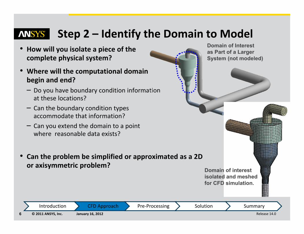
Step 2 – Identify the Domain to Model• How will you isolate a piece of the complete physical system?

• Where will the computational domain begin and end?– Do you have boundary condition information at these locations?

– Can the boundary condition types accommodate that information?

– Can you extend the domain to a point where reasonable data exists?

• Can the problem be simplified or approximated as a 2Dor axisymmetric problem?


Domain of Interestas Part of a LargerSystem (not modeled)

Domain of interestisolated and meshedfor CFD simulation.


Step 3 – Create a Solid Model• How will you obtain a model of the fluid region?– Make use of existing CAD models?– Extract the fluid region from a solid part?– Create from scratch?

• Can you simplify the geometry?– Remove unnecessary features that would complicate meshing (fillets, bolts…)?

– Make use of symmetry or periodicity if both the solution and boundary conditions are symmetric / periodic?

• Do you need to split the model so that boundary conditions or domains can be created?



Step 4 – Design and Create the Mesh• What degree of mesh resolution is required in each region of the domain?– Can you predict regions of high gradients?

• The mesh must resolve geometric features of interest and capture gradients of concern, e.g. velocity, pressure, temperature gradients

– Will you use adaption to add resolution

• What type of mesh is most appropriate?– How complex is the geometry?– Can you use a quad/hex mesh or is tri/tet more suitable?– Are non‐conformal interfaces needed?

• Do you have sufficient computer resources?– How many cells/nodes are required?– How many physical models will be used?



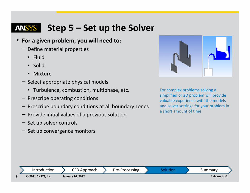
Step 5 – Set up the Solver• For a given problem, you will need to:– Define material properties

• Fluid• Solid• Mixture

– Select appropriate physical models• Turbulence, combustion, multiphase, etc.

– Prescribe operating conditions– Prescribe boundary conditions at all boundary zones– Provide initial values of a previous solution– Set up solver controls– Set up convergence monitors


For complex problems solving a simplified or 2D problem will provide valuable experience with the models and solver settings for your problem in a short amount of time


Step 6 – Compute the Solution• The discretized conservation equations are solved iteratively until convergence

• Convergence is reached when:– Changes in solution variables from one iteration to the next are negligible• Residuals provide a mechanism to help monitor this trend

– Overall property conservation is achieved• Imbalances measure global conservation

– Quantities of interest (e.g. drag, pressure drop) have reached steady values• Monitor points track quantities of interest

• The accuracy of a converged solution depends on– Appropriatenes and accuracy of physical models– Mesh resolution and independence– Numerical errors


A converged and mesh‐independent solution on a well‐posed problem will provide useful engineering results!


Step 7 – Examine the Results• Examine the results to review solution and extract useful data

• Visualization Tools can be used to answer such questions as:– What is the overall flow pattern?– Is there separation?– Where to shocks, shear layers, etc. form?– Are key flow features being resolved?

• Numerical Reporting Tools can be used to calculate quantitative results:– Forces and Moments– Average heat transfer coefficients– Surface and Volume integrated quantities– Flux Balances


Examine results to ensure property conservation and correct physical behavior. High residuals may

be caused by just a few poor quality cells.


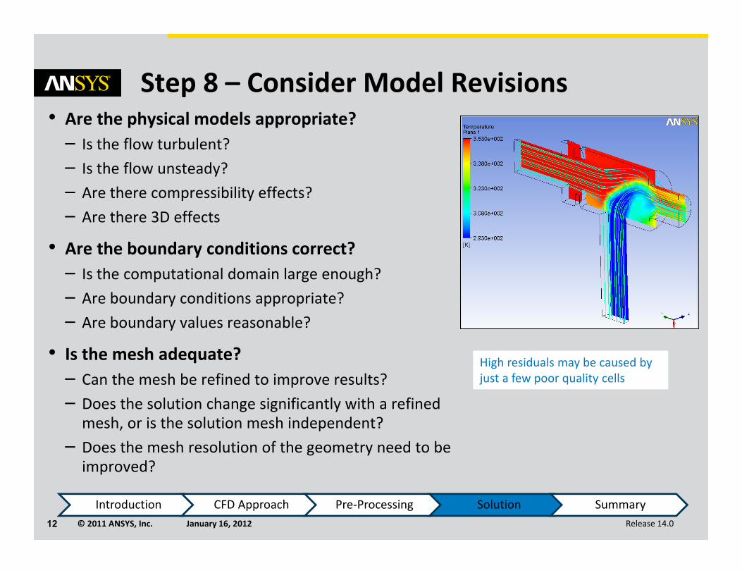
Step 8 – Consider Model Revisions• Are the physical models appropriate?– Is the flow turbulent?– Is the flow unsteady?– Are there compressibility effects?– Are there 3D effects

• Are the boundary conditions correct?– Is the computational domain large enough?– Are boundary conditions appropriate?– Are boundary values reasonable?

• Is the mesh adequate?– Can the mesh be refined to improve results?– Does the solution change significantly with a refined mesh, or is the solution mesh independent?

– Does the mesh resolution of the geometry need to be improved?


High residuals may be caused by just a few poor quality cells


Summary and Conclusions• All CFD simulations (in all mainstream CFD software products) are approached using the steps just described

• Remember to first think about what the aims of the simulation are prior to creating the geometry and mesh

• Make sure the solver is applying the appropriate physical models, and that the simulation is fully converged (more in a later lecture)

• Examine the results carefully– You may need to rework some of the earlier steps in light of the flow field predicted by CFD

• Next step:– Your instructor will now demonstrate CFX in action



Introduction to CFX• The remainder of the lecture will now focus on CFX, covering the following topics– Launching CFX, either inside or outside of ANSYS Workbench– A typical CFD study workflow performed with CFX– A summary of files and file types– An instructor demo of a simple CFD project

Introduction Launching CFX Workflow Files Demo


Running Standalone vs Workbench• Running CFX inside the Workbench environment:

– Simplifies the workflow• Geometry, Mesh, Setup, Solution and Results steps shown on the Project Schematic

• Easier to update a project when a change is made– E.g. after a geometry change a single click updates the Mesh, Setup, Solution and Results

– Allows you to easily link to other Analysis Systems and Components

– Is necessary when performing DesignExploration (parametric studies)



Running Standalone vs Workbench• Running CFX standalone:

– Less computational overhead

– Produces a simpler directory / file structure on disk

– But no direct association between geometry, mesh, setup and results files• Each component must be updated• No built‐in automation for parametric studies

– Less automation• E.g mesh needs to be manually imported into CFX‐Pre



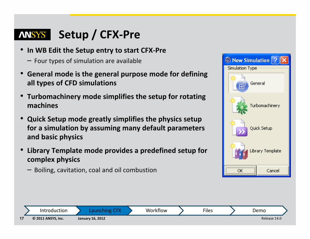
Setup / CFX‐Pre• In WB Edit the Setup entry to start CFX‐Pre– Four types of simulation are available

• General mode is the general purpose mode for defining all types of CFD simulations

• Turbomachinery mode simplifies the setup for rotating machines

• Quick Setup mode greatly simplifies the physics setup for a simulation by assuming many default parameters and basic physics

• Library Template mode provides a predefined setup for complex physics– Boiling, cavitation, coal and oil combustion



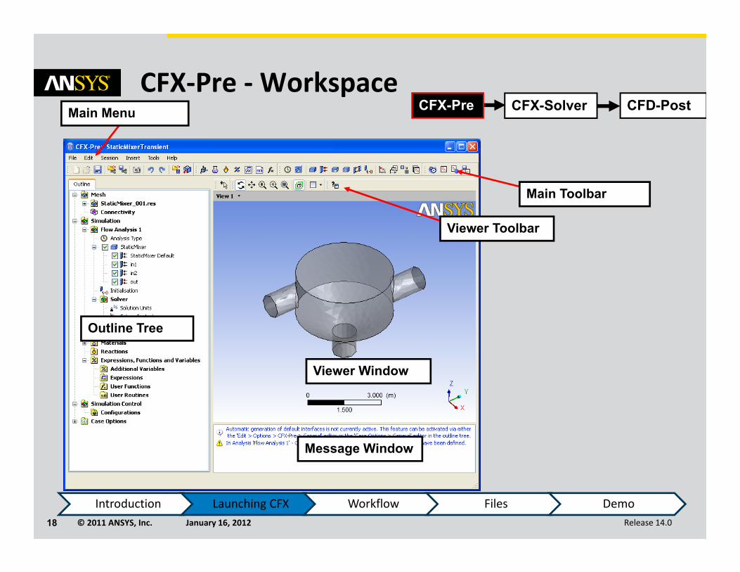
CFX‐Pre ‐Workspace

Outline Tree

Viewer Window

Main Menu

Message Window

Viewer Toolbar

Main Toolbar

CFD-PostCFX-Pre CFX-Solver



CFX‐Pre ‐Workflow

• To define your simulation, generally follow the Outline tree from top to bottom

• Double‐click entries in the Outline tree to edit

• Right‐click on entries in the Outline tree to insert new items or perform operations

• Some items are optional, depending on your simulation

Mesh and region control

• Import, delete, transform meshes

• View & edit mesh regions

Library objects• Optional. Referenced elsewhere in the setup• Import Materials & Reactions from libraries provided• Insert Expressions, AV’s, Fortran routines

Solver settings• Convergence controls• Results files controls• Numerical schemes• Monitor points

Initialisation• Starting point for the

solver in the absence of a previous solution

Boundary Conditions

Domain• Right-click to insert

boundary conditions

Analysis Type• Steady State /

Transient

CFD-PostCFX-Pre

CFX-Solver



Useful Shortcuts

Viewer Toolbar

Rotate

Pan + CTRL

Zoom + SHIFT

Box Zoom

Rotate(on screen plane)

+ CTRL

(Hold while tracing a box)



CFX‐Pre – Workflow Example• Load Mesh– Right‐click on ‘Mesh’

A Default Domain is automatically created when the mesh is imported. It contains all 3D regions in the mesh.Every domain contains a default boundary condition.




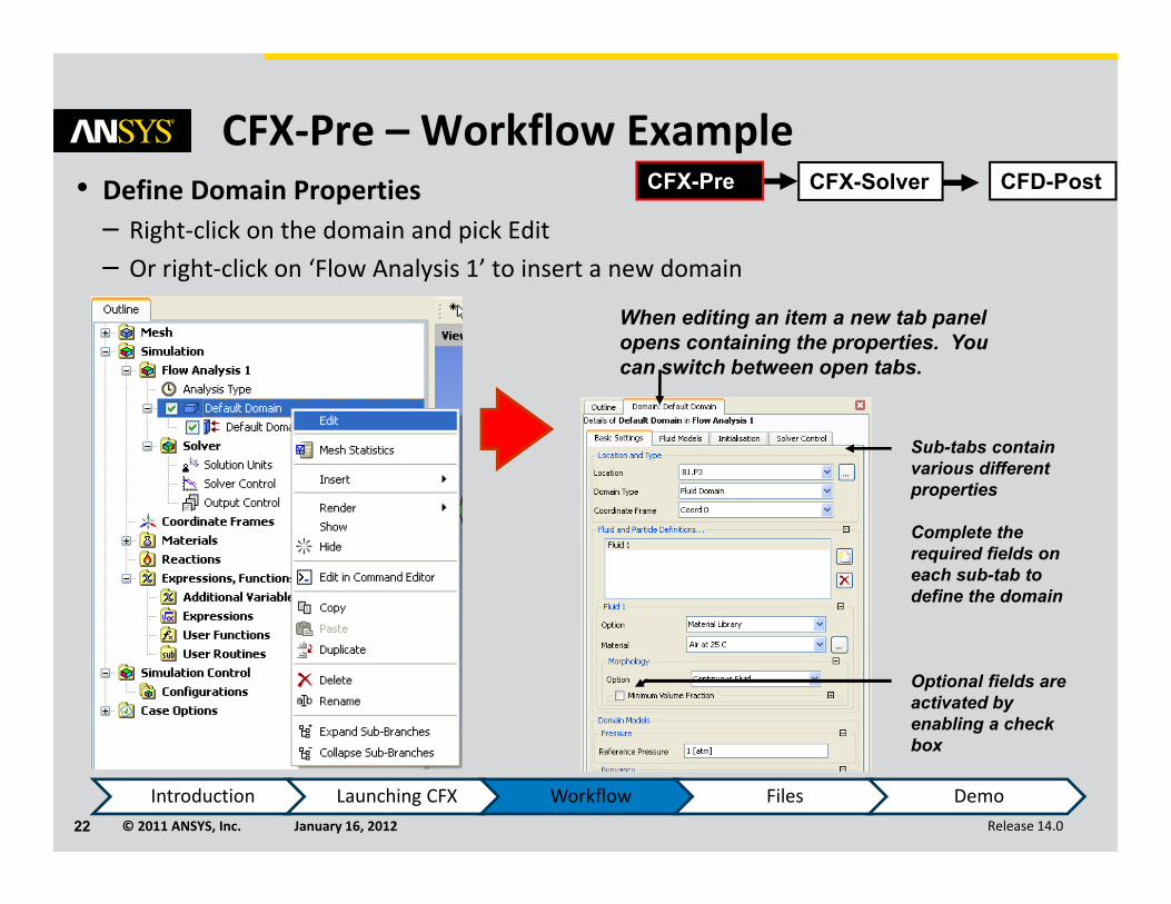
CFX‐Pre – Workflow Example• Define Domain Properties– Right‐click on the domain and pick Edit– Or right‐click on ‘Flow Analysis 1’ to insert a new domain

When editing an item a new tab panel opens containing the properties. You can switch between open tabs.

Sub-tabs contain various different properties

Complete the required fields on each sub-tab to define the domain

Optional fields are activated by enabling a check box




CFX‐Pre – Workflow Example• Create Boundary Conditions– Right‐click on the domain to insert BC’s


After completing the boundary condition, it appears in the Outline tree below its domain



CFX‐Pre – Workflow Example• Define Solver Settings– Right‐click on Solver Control and pick Edit


All solver controls have default values



CFX‐Pre – Workflow Example• Start Solver– When running in Workbench:

• Just close CFX‐Pre– Files are automatically saved– Check mark shown next to Setup

• Right‐click on Solution and select Edit or Refresh– Referesh runs the solver in the background with default settings

– Edit opens the Solver Manager


– When running in Workbench:• You should manually save the CFX‐Pre database

• Right‐click on Simulation and select ‘Start Solver’– Define Run opens the Solver Manager

– Run Solver runs in the background with default settings

– Run Solver and Monitor run with default settings and monitors in the Solver Manager

Right-click to solve



CFX Solver Manager• Defining a Run– CFX‐Pre will have written a .def file and this is automatically selected as the Solver Input File

– Can enable Initial Values check box if you have a previous solution to use as the starting point

– Parallel settings are defined here• Allows you to divide a large CFD problem so that it can run on more than one processor/machine

– Start Run




CFX Solver Manager• Workspace CFD-PostCFX-Pre CFX-Solver

Solution Monitors• Monitor the convergence of

the solver• Plot residuals, imbalances,

monitor points, forces, fluxes…

Text output from the Solver• Lots of info in here• Can also view the .out file in

a text editor

Create new monitors



CFX Solver Manager• When the Solver finishes, start CFD‐Post

• When running in Workbench:– Just close the Solver Manager

• Check mark shown next to Solution– Right‐click on Results and select Edit to start CFD‐Post


• When running in Workbench:– Enable Post‐Process Results on the solver finished notification window

– Or select the Post‐Process Results icon from the toolbar

Right-click to start CFD-Post



CFD‐Post• Workspace CFX-Pre CFD-PostCFX-Solver

Outline Tree

Viewer WindowDetails Pane

Outline tree displays all post-processing objects. Right-click or double-click to edit in the Details Pane

Editor Tabs• Outline• Variables• Expressions• Calculators• Turbo



CFD‐Post• General Workflow

• Prepare locations where data will be extracted from, or plots generated– E.g. Planes, Isosurface

• Create variables/expressions which will be used to extract data (if necessary)– E.g. Drag, pressure ratio

CFX-Pre CFD-PostCFX-Solver

• Generate qualitative data at locations

• Generate quantitative data at locations

• Generate Reports



CFD‐Post• Create Locations

• Variables

• Qualitative and Quantitative data

• Reports

CFX-Pre CFD-PostCFX-Solver

Use the Locationdrop-down menu in the toolbar to create locations inside the domain

2D & 3D domain, boundary and mesh regions are automatically available

Discussed in the Post-processing lecture along with more details on creating locations



Common File Types

CFX-Solver

CFX-Pre

CFD-Post

.def (Solver Input or Definition File)

.cfx (CFX-Pre Database)

.wbpj (Workbench Project File)

.out (Solver Output File)

.res (Results File)

.cst (CFD-Post State File)

.cse (CFD-Post Session File).def, .cmdb(Mesh Files)

Import Mesh.cmdb, .cfx5, .def, .res, …

Open.cfx, .def, .res



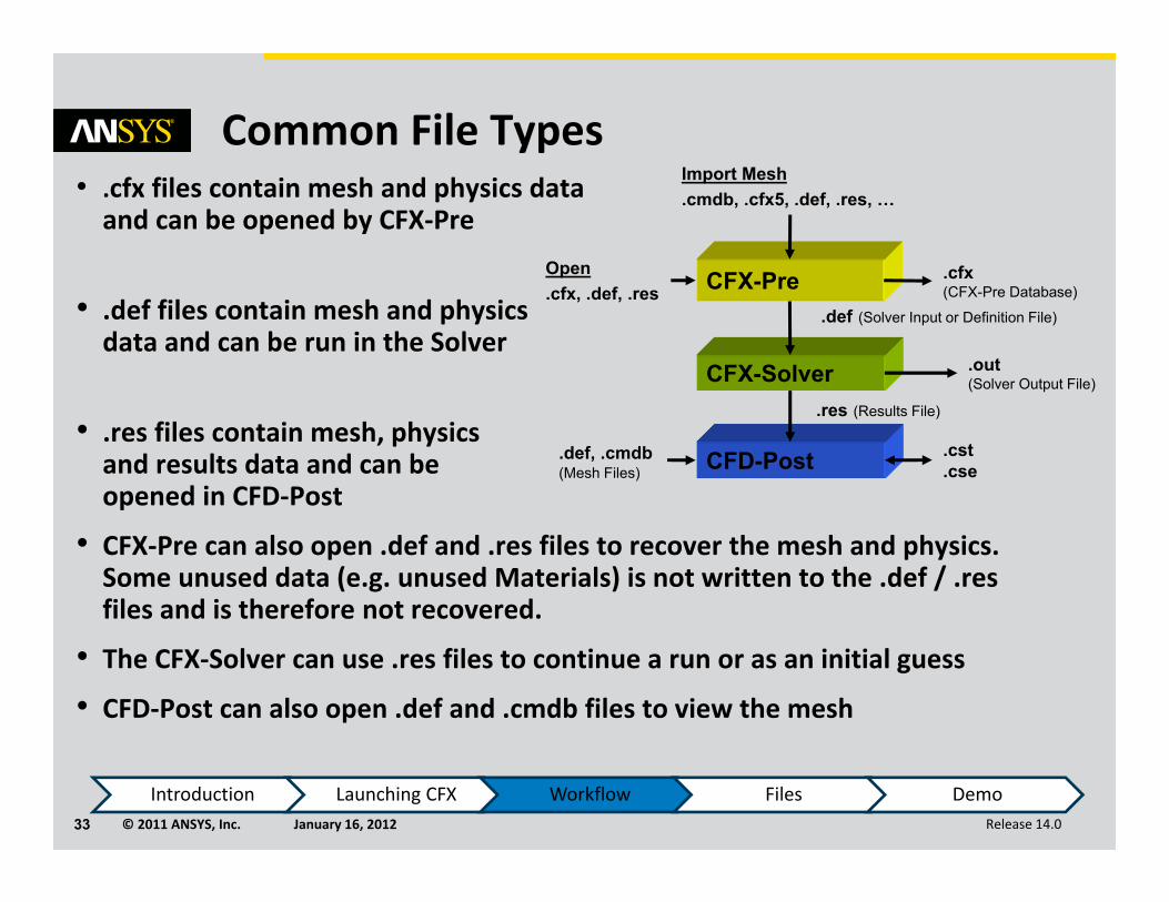
Common File Types• .cfx files contain mesh and physics data and can be opened by CFX‐Pre

• .def files contain mesh and physics data and can be run in the Solver

• .res files contain mesh, physics and results data and can be opened in CFD‐Post

• CFX‐Pre can also open .def and .res files to recover the mesh and physics. Some unused data (e.g. unused Materials) is not written to the .def / .res files and is therefore not recovered.

• The CFX‐Solver can use .res files to continue a run or as an initial guess

• CFD‐Post can also open .def and .cmdb files to view the mesh

CFX-Solver

CFX-Pre

CFD-Post

.def (Solver Input or Definition File)

.cfx(CFX-Pre Database)

.out(Solver Output File)

.res (Results File)

.cst

.cse.def, .cmdb(Mesh Files)

Import Mesh.cmdb, .cfx5, .def, .res, …

Open.cfx, .def, .res



Solver Files and Folders

CFX-Solver

C:\Filename.def

C:\Filename_001.out

C:\Filename_001

C:\Filename_001\100_full.bak

C:\Filename_001\1.trnC:\Filename_001\2.trn

C:\Filename_001.res

First Time Solving Filename.def

CFX-Solver

C:\Filename.def

C:\Filename_002.out

C:\Filename_002

C:\Filename_002\100_full.bak

C:\Filename_002\1.trnC:\Filename_002\2.trn

C:\Filename_002.res

Second Time Solving Filename.def



File Structure in Workbench• When running CFX standalone, files are saved to your current working directory– As noted on the previous side, some solver files are saved to a solver run directory

• When running in Workbench only the project file (.wbpj) is saved to the current working directory– All other files are saved to a name_files subdirectory

C:\StaticMixer.wbpj

C:\StaticMixer_files

Project files and folders. Do not edit directly



Workflow Demo• Your instructor will now perform a quick demonstration of the workflow in a simple CFX project

• This simulation sets up the Static Mixer simulation – the first of the tutorials supplied with the ANSYS CFX documentation

• The mesh for this simulation can be found in the examples directory of your CFX installation and can be imported as a CFX‐Solver Input mesh file– By default: C:\Program Files\ANSYS Inc\v130\CFX\examples\StaticMixer.def


cfx-intro_14.0_l02_introcfd_cfx

Documents

solver output file

outline tree

results file

definition file

ctrl

solver input

pre database

solver cfd