cger’s supercomputer monograph report volcger.nies.go.jp/publications/report/i143/i143.pdf ·...
TRANSCRIPT

Center for Global Environmental Research
National Institute for Environmental Studies, Japan
CG
ER
’S SUPE
RC
OM
PUT
ER
MO
NO
GR
APH
RE
POR
T V
ol.25
CGER-REPORT ISSN 2434-5679CGER-I143-2019
CG
ER-I143-2019
CGER’S SUPERCOMPUTER MONOGRAPH REPORT Vol.25
Transport modeling algorithms for application of the GOSATobservations to the global carbon cycle modeling
Shamil Maksyutov, Tomohiro Oda, Makoto Saito, Hiroshi Takagi, Dmitry Belikov and Vinu Valsala


Center for Global Environmental Research
National Institute for Environmental Studies, Japan
CGER-REPORT ISSN 2434-5679CGER-I143-2019
CGER’S SUPERCOMPUTER MONOGRAPH REPORT Vol.25
Transport modeling algorithms for application of the GOSATobservations to the global carbon cycle modeling
Shamil Maksyutov, Tomohiro Oda, Makoto Saito, Hiroshi Takagi, Dmitry Belikov and Vinu Valsala

CGER’S SUPERCOMPUTER MONOGRAPH REPORT Vol.25 Transport modeling algorithms for application of the GOSAT observations to the global carbon cycle modeling Shamil Maksyutov, Tomohiro Oda, Makoto Saito,
Hiroshi Takagi, Dmitry Belikov and Vinu Valsala Edited by:
Center for Global Environmental Research (CGER) National Institute for Environmental Studies (NIES)
Coordination for Resource Allocation of the Supercomputer:
Center for Global Environmental Research (CGER) National Institute for Environmental Studies (NIES)
Supercomputer Steering Committee (FY2018):
Masayoshi Ishii (Meteorological Research Institute, Japan Meteorological Agency) Masaki Satoh (Atmosphere and Ocean Research Institute, The University of Tokyo) Hisashi Yashiro (Computional Climate Science Research Team, RIKEN AICS) Akinori Takami (Center for Regional Environmental Research/NIES) Norihiko Tanaka (Planning Department /NIES) Hideharu Akiyoshi (Center for Global Environmental Research /NIES) Seita Emori (Center for Global Environmental Research/NIES)
Maintenance of the Supercomputer System: Environmental Information Department (EID) National Institute for Environmental Studies (NIES)
Operation of the Supercomputer System: NEC Corporation
Copies of this report can be obtained from:
Center for Global Environmental Research (CGER) National Institute for Environmental Studies (NIES) 16-2 Onogawa, Tsukuba, Ibaraki , 305-8506 Japan Fax: +81-29-858-2645 E-mail: [email protected]
Copyright 2019:
NIES: National Institute for Environmental Studies
This publication is printed on paper manufactured entirely from recycled material (Rank A), in accordance with the Law Concerning the Promotion of Procurement of Eco-Friendly Goods and Services by the State and Other Entities.
ISSN 2434- 5679 (online Version), CGER-I143-2019

i
Foreword
The Center for Global Environmental Research (CGER) at the National Institute for Environmental Studies (NIES) was established in October 1990, with the main objectives of contributing to the scientific understanding of global environmental change and identifying solutions to critical environmental problems. CGER conducts environmental research from an interdisciplinary, multi-agency, and international perspective, and provides an intellectual infrastructure for research activities in the form of databases and a supercomputer system. CGER also ensures that data from its long-term monitoring of the global environment is made available to the public.
CGER installed its first supercomputer system (NEC SX-3, Model 14) in March 1992, and this was subsequently upgraded to an NEC Model SX-4/32 in 1997, an NEC Model SX-6 in 2002, an NEC Model SX-8R/128M16 in 2007, and an NEC Model SX-9/A(ECO) in June 2013. In June 2015, the system was further upgraded with the inclusion of an NEC Model SX-ACE, in order to provide an increased capacity for speed and storage.
The supercomputer system is available for use by researchers from NIES and other research organizations and universities in Japan. The Supercomputer Steering Committee consists of leading Japanese scientists in climate modeling, atmospheric chemistry, ocean environment, computer science, and other areas concerned with global environmental research, and one of its functions is to evaluate proposals of any research requiring the use of the Supercomputer system.
To promote the dissemination of results, we publish both an Annual Report and occasional Monograph Reports. Annual Reports deliver results for all research projects that have made use of the supercomputer system in a given year, while Monograph Reports present the integrated results of a particular research program.
This Monograph Report provides an overview of developing transport model, gridded anthropgenic emission inventory and inverse modeling for using observations by Japanese Greenhouse Gas Observing Satellite (GOSAT) to produce Level 4 product – regional CO2 fluxes estimated based on surface and satellite observations of atmospheric CO2.
In the years to come we intend to continue our support of environmental research by enabling the use of our supercomputer resources, and continue to disseminate practical information based on our results. January 2019
Nobuko Saigusa Director
Center for Global Environmental Research National Institute for Environmental Studies
- i -

ii
Preface
Keeping the anthropogenic greenhouse gas (GHG) emissions under control has been a long-standing objective on international stage for several decades. This objective was addressed by adopting Kyoto and Paris climate agreements. Accurate reporting and verification of the national antropogenic emissions is important component of the treaty implementation. Atmopsheric observations serve as basis for independent, top-down assessment of the emissions and sinks estimated with inventories and models. Inverse modeling of the surface greenhouse gas fluxes is a widely used method to estimate the regional sources and sinks based on matching the observed atmospheric concentrations with atmospheric transport model simulation. In 2009, the global greenhouse gas observing system was enhanced by putting on orbit a Japanese Greenhouse Gas Observing SATellite (GOSAT), which provided significant improvement in accuracy over other satellites, and created many new opportunities for observing global carbon and methane cycles. Global coverage of GOSAT and higher accuracy provides a lot of benefits, that attracted a number of user groups. On the other hand, several new challenges for atmospheric and surface flux modelers have arrived. Accurate simulation of the stratospheric CO2 and methane profiles is required for matching with GOSAT total column measurements. Developing operational inversion system requires that the surface flux datasets, meteorlogical reanalysis data are reliably updated withing one year of receiving the observational data. Ability of GOSAT to observe not only clean, background air, but also air influenced by man-made, antropogenic emissions, open opportunies for monitoring the meissions and their trends. That objective demands development of the new high resolution atmophseric transport models and inverse modeling techniques.
In this monograph, we report development of the models and inventories for GOSAT data analysis and applications, including the atmospheric transport model, high resolution carbon dioxide emission inventory, the methodology of the GOSAT Level 4 product and development of the high resolution transport modeling tools intended for inverse modeling of antropgenic emissions using the satellite observations. This monograph is based on the following four papers.
[Chapter 1] Simulations of column-averaged CO2 and CH4 using the NIES TM with a hybrid sigma-isentropic (sigma-theta) vertical coordinate, by Belikov, D. A., Maksyutov, S., Sherlock, V., Aoki, S., Deutscher, N. M., Dohe, S., Griffith, D., Kyro, E., Morino, I., Nakazawa, T., Notholt, J., Rettinger, M., Schneider, M., Sussmann, R., Toon, G. C., Wennberg, P. O., and Wunch, D., Atmospheric Chemistry and Physics, 13, 1713-1732, 10.5194/acp-13-1713-2013, 2013.
[Chapter 2] The Open-source Data Inventory for Anthropogenic CO2, version 2016 (ODIAC2016): a global monthly fossil fuel CO2 gridded emissions data product for tracer transport simulations and surface flux inversions, by Oda, T., Maksyutov, S., and Andres, R. J.: Earth System Science Data, 10, 87-107, 10.5194/essd-10-87-2018, 2018.
[Chapter 3] Regional CO2 flux estimates for 2009-2010 based on GOSAT and ground-based CO2 observations, by Maksyutov, S., Takagi, H., Valsala, V. K., Saito, M., Oda, T., Saeki, T., Belikov, D. A., Saito, R., Ito, A., Yoshida, Y., Morino, I., Uchino, O., Andres, R. J., and Yokota, T.:, Atmospheric Chemistry and Physics, 13, 9351-9373, 10.5194/acp-13-9351-2013, 2013.
- ii -

iii
[Chapter 4] Adjoint of the global Eulerian-Lagrangian coupled atmospheric transport model (A-GELCA v1.0): development and validation, by Belikov, D. A., Maksyutov, S., Yaremchuk, A., Ganshin, A., Kaminski, T., Blessing, S., Sasakawa, M., Gomez-Pelaez, A. J., and Starchenko, A.: Geoscientific Model Development, 9, 749-764, 10.5194/gmd-9-749-2016, 2016.
Chapter 1 introduces development of the atmospheric transport model utilizing an
isentropic vertical grid in stratosphere, designed to simulate realistic vertical profile of the greenhouse gases CO2 and CH4 in stratosphere and whole atmospheric column average as observed by remote sensing. Chapter 2 describes a gridded inventory of the fossil fuel emissions capable of high resolution and global coverage and available with annual updates. Chapter 3 introduces a short version of the GOSAT Level 4 product algorithm – estimating regional CO2 fluxes using GOSAT and surface observations of atmospheric CO2. Chapter 4 introduces a further development of a coupled Eulerian-Lagrangian transport model, suitable for estimationg the antropogenic emissions with ground-based and satellite data taken closer to emission sources, due to flexible choice of the spatial resolution and high resolution capability.
The authors hope that this effort will contribute to further progress in carbon cycle reseatch and use of greenhouse gas observaing satellites in understanding greenhouse gas cycles.
January 2019
Shamil Maksyutov Specialist
Satellite Observation Center Center for Global Environmental Research
National Institute for Environmental Studies
- iii -

iv - iv -

v
Contents
Foreword ..................................................................................................................................... i Preface ....................................................................................................................................... ii Contents ...................................................................................................................................... v List of Figures ........................................................................................................................ viii List of Tables ........................................................................................................................... xiv Chapter 1 Simulations of column-averaged CO2 and CH4 using the NIES TM with a hybrid sigma-isentropic (sigma-theta) vertical coordinate ................................................... 1 Abstract ....................................................................................................................................... 2 1.1 Introduction ........................................................................................................................... 3 1.2 Model description ................................................................................................................. 5 1.2.1 Sigma–isentropic vertical coordinate ................................................................................. 5 1.2.2 Simulation of upward motion in the stratosphere .............................................................. 6 1.2.3 Meteorological data and vertical resolution ....................................................................... 7 1.2.4 Turbulent diffusion and deep convection parameterization ............................................... 7 1.2.5 Model setup ........................................................................................................................ 8 1.3 Results ................................................................................................................................... 9 1.3.1 Validation of the mean age of air in the stratosphere ........................................................ 9 1.3.2 Validation of CO2, CH4, and SF6 vertical profiles in the stratosphere ............................. 11 1.3.3 Validation of CO2, CH4, and SF6 concentrations in the free troposphere ........................ 12 1.3.3.1 Validation of near-surface CH4 concentrations ............................................................ 13 1.3.3.2 Validation of CH4 vertical profiles in the troposphere ................................................. 17 1.3.4 Validation of CO2 and CH4 column-averaged DMFs ...................................................... 19 1.3.4.1 Modelled XCH4 compared with TCCON FTS observations ........................................ 20 1.3.4.2 Modelled XCO2 compared with TCCON FTS observations and GECM ..................... 25 1.4 Discussion ........................................................................................................................... 27 1.5 Conclusions ......................................................................................................................... 28 Acknowledgements ................................................................................................................... 29 References ................................................................................................................................. 30 Chapter 2 The Open-source Data Inventory for Anthropogenic Carbon dioxide (CO2), version 2016 (ODIAC2016): A global, monthly fossil-fuel CO2 gridded emission data product for tracer transport simulations and surface flux inversions ................................................................................................................................. 35 Abstract ..................................................................................................................................... 36 2.1 Introduction ......................................................................................................................... 37 2.2 Emission modeling framework ........................................................................................... 38 2.3 Emission estimates and input emission data preprocessing ................................................ 40
- v -

vi
2.3.1 Emissions for 2000-2013 ................................................................................................. 40 2.3.2 Emissions for 2014-2015 ................................................................................................. 41 2.3.3 CDIAC emission sector to ODIAC emission categories ................................................. 41 2.4. Spatial emission disaggregation ......................................................................................... 42 2.4.1 Emissions from point sources, non-point sources and cement production ...................... 42 2.4.2 Emissions from gas flaring .............................................................................................. 42 2.4.3 Emissions from international aviation and marine bunker .............................................. 43 2.5. Temporal emission disaggregation .................................................................................... 43 2.6. Results and discussions ...................................................................................................... 43 2.6.1 Annual global emissions .................................................................................................. 43 2.6.2 Global emission spatial distributions ............................................................................... 47 2.6.3 Regional emission time series. ......................................................................................... 52 2.7. Current limitations, caveats and future prospects .............................................................. 54 2.7.1 Emission estimates ........................................................................................................... 54 2.7.2 Emission spatial distributions .......................................................................................... 55 2.7.2.1 Point source emissions .................................................................................................. 55 2.7.2.2 Non-point source emissions .......................................................................................... 55 2.7.2.3. Aviation emissions ....................................................................................................... 56 2.7.3 Emission temporal profiles. ............................................................................................. 56 2.7.4 Uncertainties associated with gridded emission fields .................................................... 57 2.8. Product distribution, data policy and future update ........................................................... 58 2.9. Summary ............................................................................................................................ 58 Appendix 2.A ............................................................................................................................ 59 Appendix 2.A2 .......................................................................................................................... 60 Appendix 2.A3 .......................................................................................................................... 61 Acknowledgements ................................................................................................................... 61 References ................................................................................................................................. 61 Chapter 3 Regional CO2 flux estimates for 2009–2010 based on GOSAT and ground- based CO2 observations .......................................................................................................... 67 Abstract ..................................................................................................................................... 68 3.1 Introduction ......................................................................................................................... 69 3.2 Inverse modeling system components ................................................................................ 70 3.2.1 Model of the carbon cycling in the terrestrial biosphere. ................................................ 70 3.2.2 Variational assimilation system for simulating the global pCO2 maps and surface ocean-atmosphere fluxes of carbon. ............................................................................. 74 3.2.3 Emissions dataset for fossil fuel CO2 emissions. ............................................................. 76 3.2.4 Emissions of CO2 by biomass burning and forest fires. .................................................. 77 3.2.5 Atmospheric tracer transport model ................................................................................. 78 3.3 Inverse modeling scheme .................................................................................................... 79 3.3.1 GOSAT XCO2 retrievals .................................................................................................... 82 3.3.2 Treatment of GOSAT averaging kernel ........................................................................... 85 3.4 Results and discussion ........................................................................................................ 86 3.5 Summary and conclusions .................................................................................................. 95
- vi -

vii
Supplementary information ....................................................................................................... 96 Acknowledgements ................................................................................................................... 96 References ................................................................................................................................. 97 Chapter 4 Adjoint of the Global Eulerian–Lagrangian Coupled Atmospheric transport model (A-GELCA v1.0): development and validation ...................................................... 103 Abstract ................................................................................................................................... 104 4.1 Introduction ....................................................................................................................... 105 4.2 Model and method ............................................................................................................ 107 4.2.1 Global coupled Eulerian-Lagrangian model .................................................................. 107 4.2.2 FLEXPART ................................................................................................................... 108 4.2.3 Meteorological data ........................................................................................................ 109 4.2.3.1 Meteorological data processing for NIES TM ............................................................ 109 4.2.3.2 Meteorological data processing for FLEXPART ........................................................ 109 4.3 Inverse modeling for the flux optimization problem ........................................................ 109 4.4 Assessment of the coupled model ..................................................................................... 110 4.5 Construction and validation of the adjoint model ............................................................. 118 4.5.1 Construction ................................................................................................................... 118 4.5.2 Validation of the coupled adjoint ................................................................................... 119 4.5.2.1 Validation of the NIES TM adjoint ............................................................................. 119 4.5.2.2 Real case simulation .................................................................................................... 121 4.6 Computational efficiency .................................................................................................. 124 4.7 Summary ........................................................................................................................... 125 Code availability ..................................................................................................................... 126 Acknowledgments ................................................................................................................... 126 References ............................................................................................................................... 126 Publications, Authors, and Contact person ........................................................................ 131 Publications ............................................................................................................................. 131 Authors .................................................................................................................................... 135 Contact Person ........................................................................................................................ 135 CGER’S SUPERCOMPUTER MONOGRAPH REPORT .................................................... 137
- vii -

viii
List of Figures
Chapter 1 Figure 1.1 Mean age of air at 20 km altitude from NIES TM simulations (blue
line), compared with the mean age of air derived from in situ ER-2 aircraft observations of CO2 (Andrews et al., 2001) and SF6 (Ray et al., 1999) (red line). Error bars for the observations are 2 σ (Monge‐Sanz et al., 2007) ............................................................................ 10
Figure 1.2 Comparison of observed and modelled (red lines) mean age of air at latitudes of: (a) 5°S, (b) 40°N, and (c) 65°N. The lines with symbols represent observations: in situ SF6 (dark blue line with triangles) (Elkins et al., 1996; Ray et al., 1999), whole air samples of SF6 (purple line with squares for (b) panel, light blue line with squares outside vortex and orange line with asterisks inside vortex (c) panel) (Harnisch et al., 1996), and mean age from in situ CO2 (green line with diamonds) (Boering et al., 1996; Andrews et al., 2001) ......................... 10
Figure 1.3 Cross-section of the annual mean age of air (years) from NIES TM simulations of SF6 with JRA-25/JCDAS reanalysis ....................................... 11
Figure 1.4 Comparison of observed and modelled concentration averaged for the period 2000–2007: a) SF6, b) CH4, and c) CO2. The observed VMRs were derived from six individual profiles of balloon-borne measurements over Sanriku, Japan (39.17°N, 141.83°E) ............................... 12
Figure 1.5 Detrended seasonal cycle of surface CH4 volume mixing ratio for GLOBALVIEW stations (corresponding TCCON stations in parentheses): a) Baltik See (Bialystok); b) Ocean Station M (Bremen); c) Darwin (Darwin); d) Hohenpeissenberg (Garmisch); e) Izaña (Izaña); f) Southern Great Plains (Lamont); g) Baring Head Station (Lauder); h) Pic Du Midi (Orleans); i) Park Falls (Park Falls); j) Pallas-Sammaltunturi (Sodankylä); k) Ryori (Tsukuba); l) Cape Grim (Wollongong); m) Alert; n) Mauna Loa; and o) Syowa. .................................................................................................................. 14-15
Figure 1.6 Average difference between simulated and observed trends (ppb/yr) of CH4 for Jan 1990 and Dec 2009 at GLOBALVIEW stations .................... 16
Figure 1.7 Correlation coefficients between simulated and observed CH4 at GLOBALVIEW stations ................................................................................ 17
Figure 1.8 Comparison of observed and modeled CH4 concentrations averaged for the period 1993-2007 over Surgut, West Siberia. The vertical profiles were produced by averaging the modelled and observed concentrations taken on the same day and at the same time. Error bars show the standard deviation .................................................................... 18
Figure 1.9 Time series of model bias (modelled CH4 concentration minus observed) and the averaged (moving average with period 12) value of the bias for the 1, 3, and 7 km levels over Surgut (61.25°N, 73.43°E) for the period 1993–2007 ................................................................ 19
Figure 1.10 Time series of XCH4 measured by FTS and modelled by NIES TM for the period January 2009 to February 2011, for the following stations: a) Bialystok (Poland, 53.22°N, 23.13°E); b) Bremen (Germany, 53.10°N, 8.85°E); c) Darwin (Australia, 12.42°S, 130.89°E); d) Garmisch (Germany, 47.48°N, 11.06°E); e) Izaña
- viii -

ix
(Spain, 28.30°N, 16.50°W); f) Lamont (USA, 36.6°N, 97.49°W); g) Lauder (New Zealand, 45.04°S, 169.68°E); h) Orleans (France, 47.97°N, 2.11°E); i) Park Falls (USA, 45.95°N, 90.27°W); j) Sodankylä (Finland, 67.37°N, 26.63°E); k) Tsukuba (Japan, 36.05°N, 140.12°E); and l) Wollongong (Australia, 34.41°S, 150.88°E). The “error” for each symbol is a combination of the spread due to weighted averaging within the 13:00 ± 1 hour local time interval and observation error ........................................................... 22-23
Figure 1.11 Scatter diagram of modelled and FTS XCH4 at all FTS sites. Dotted lines show a standard deviation of ±1% of XCH4 .......................................... 24
Figure 1.12 Time series of XCO2 measured by FTS, modelled by NIES TM and derived from a 3-D CO2 climatology GECM for the period January 2009 to February 2011, for the following stations: a) Bialystok (Poland, 53.22°N, 23.13°E); b) Bremen (Germany, 53.10°N, 8.85°E); c) Darwin (Australia, 12.42°S, 130.89°E); d) Garmisch (Germany, 47.48°N, 11.06°E); e) Izaña (Spain, 28.30°N, 16.50°W); f) Lamont (USA, 36.6°N, 97.49°W); g) Lauder (New Zealand, 45.04°S, 169.68°E); h) Orleans (France, 47.97°N, 2.11°E); i) Park Falls (USA, 45.95°N, 90.27°W); j) Sodankylä (Finland, 67.37°N, 26.63°E); k) Tsukuba (Japan, 36.05°N, 140.12°E); and l) Wollongong (Australia, 34.41°S, 150.88°E). The “error” for each symbol is a combination of the spread due to weighted averaging within the 13:00 ± 1 hour local time interval and observation error ......... 26-27
Chapter 2 Figure 2.1 A schematic figure of the ODIAC emission modeling framework
(defined as “ODIAC 3.0 FFCO2 model”). Starting with CDIAC national emission estimates made by fuel type (emission estimates), the CDIAC national emission estimates are first divided into extended ODIAC emission categories (input data processing, see Section 2.3). ODIAC 3.0 FFCO2 model then distributes the emissions in space and time, using point source geolocation information and spatial data depending on emission category such as nighttime light (NTL), and aircraft and ship fleet tracks (spatial disaggregation, see Section 2.4). The emission seasonality for emissions over land and international aviation were adopted from existing emission inventories (temporal disaggregation, see Section 2.5) .................................................................................................................. 39
Figure 2.2 Global emission time series from four gridded emission data: CDIAC (red, 2000-2013) plus projected emissions (dashed maroon, 2014-2015) (values taken from ODIAC2016), CDIAC 1×1 degree (black, 2000-2013), EDGAR v4.2 (green, 2000-2008) and EDGAR v4.2 Fast Track (blue, 2000-2010). The values here are given in the unit of peta gram (= giga tonnes) carbon per year. The shaded area indicated in tan is a two-sigma uncertainty range (8%) estimated for CDIAC global total emission estimates by Andres et al. (2014) .................... 44
Figure 2.3 National emission time series for top 10 emitting countries (China, U.S., India, Russian Federation, Japan, Germany, Islamic Republic of Iran, Republic of Korea (South Korea), Saudi Arabia and Brazil). The values are given in the unit of peta gram (=giga tonnes) carbon
- ix -

x
per year. The values are calculated using gridded emission data, not tabular emission data. The national total values in the plots might be thus different from values indicated in the tabular form due to the emission disaggregation. The shaded area in grey indicates a two-sigma uncertainty range estimated by Andres et al. (2014) (see Table 2.2) .................................................................................................................. 46
Figure 2.4 Year 2013 global fossil fuel CO2 emissions distributions from CDIAC (left, 8.36 PgC) and ODIAC (right, 9.78 PgC). The ODIAC emission field was aggregated to a common 1 × 1 degree resolution. The value is given in the unit of log of thousand tonnes C/cell ...................... 48
Figure 2.5 Year 2013 global distributions of ODIAC fossil fuel emissions by emission type. The panels show emissions from (from top to the right, then down) point source, non-point source, cement production, gas flaring, international aviation and international shipping. The values in the figures are given in the unit of log of thousand tonnes carbon/year/cell (1×1 degree). The numbers in the brackets are the total for the category emissions in the unit of PgC (total year 2013 emission in ODIAC2016 was 9.78 PgC) ........................................................ 48
Figure 2.6 Land emissions from ODIAC (upper left), CDIAC (upper right), two versions of EDGAR emission data (v4.2 lower left and v4.2 Fast Track lower right). The units are million tonnes carbon/year/cell (1×1 degree). In addition to excluding emissions from international aviation and marine bunker, some of the sector emissions were subtracted from EDGAR short cycle total emissions to account for the differences in emission calculation methods between CDIAC and EDGAR, as also done earlier. The emission fields for the year 2008 were used ............................................................................................... 50
Figure 2.7 ODIAC-other emission data differences. CDIAC (upper right), two versions of EDGAR (v4.2 lower left and v4.2 Fast Track lower right). The units are million tonnes carbon/year/cell (1×1 degree). Note that the differences are defined as ODIAC (this study) minus others. The histograms of the differences are also presented in Appendix A3 ................................................................................................... 51
Figure 2.8 Emission time series over inversion analysis land regions defined by the Transport model intercomparison (TransCom) project (Gurney et al., 2002). The TransCom region map (bottom right) is available from http://transcom.project.asu.edu/transcom03_protocol_basisMap.php (last access: 8 November, 2016). Black lines indicate the ODIAC 1×1 degree monthly emissions. The monthly emissions are calculated using the 1×1 degree ODIAC emission data. The uncertainty range was calculated by mass weighted uncertainty estimates of countries that fall into the regions (see Table 2.3). The uncertainty ranges shown in Fig. 2.8 are annual uncertainty plus the monthly profile uncertainty (12.8%, reported by Andres et al., 2011). Note scales in the vertical axis are different ................................................... 53
Appendix Figure 2.A3 A histogram of the inter-emission data differences from ODIAC. Values are given in the unit of million tonnes carbon per year (MTC/yr) ......................................................................................................... 61
- x -

xi
Chapter 3
Figure 3.1 Comparison of the optimized VISIT model results to the observations. Top: forward simulation of atmospheric CO2 (ppm) at Mauna-Loa (red circles), and Globalview (blue triangles). Below: global map of gridded mean biomass (Mg C ha-1): (middle) IIASA database, (bottom) optimized VISIT .............................................................. 73
Figure 3.2 Top: June 2009 to May 2010 averaged air-to-sea CO2 prior fluxes (gC/m2/day) used in the inversion. Bottom: global integral of air-to-sea CO2 fluxes (PgC/yr) and corresponding global mean data uncertainties used in the inversion .................................................................. 75
Figure 3.3 Global distribution of the annual mean CO2 emissions due to burning fossil fuels ....................................................................................................... 77
Figure 3.4 Boundaries of the 64 source regions adopted in this study. The numbers on the figure are the region IDs of each region. Regions shaded with dark blue are not considered in the flux estimation .................... 82
Figure 3.5 The number of GOSAT Level 2 XCO2 data records per each of 5×5 grid cells during the months of August 2009, November 2009, February 2010, and May 2010. Red circles indicate the locations of the GV measurement sites chosen for this study ............................................ 84
Figure 3.6. Version 02.00 of the XCO2 retrievals in the form of input to our inverse modeling scheme (gridded to 5×5 cells and averaged on a monthly time scale). Cells with three or more retrievals per month are shown here. The bias was corrected by raising each XCO2 retrieval by 1.20 ppm. Overlaid are GLOBALVIEW values (in circles) that are also in the form of input to inverse modeling (monthly means). Values for the months of August 2009 (summer in the Northern Hemisphere), November 2009 (fall), February 2010 (winter), and May 2010 (spring) are shown ................................................... 85
Figure 3.7 Percent reduction in the uncertainty of monthly surface flux estimates, attained by adding the GOSAT XCO2 retrievals to the GLOBALVIEW dataset .................................................................................. 87
Figure 3.8 Monthly fluxes (gCm−2 day−1) estimated for the 64 subcontinental regions using GV data and GOSAT XCO2 retrievals, for the months of August 2009 (summer in the Northern Hemisphere), November 2009 (fall), February 2010 (winter), and May 2010 (spring). The value presented here are is the sum of a priori fluxes (terrestrial biosphere exchange or ocean exchange + anthropogenic emissions + forest fire emissions) and the correction to the a priori flux determined via the optimization. Note the different color-coded scales for land and ocean regions ................................................................... 88
Figure 3.9 Differences between the fluxes estimated from GV data only and those from combined GV and GOSAT XCO2 retrievals. Note the different color-coded scales for land and ocean regions ................................. 88
Figure 3.10 Time series of data collected at five TCCON sites (green), and corresponding forward simulation results based on a posteriori fluxes estimated from GV alone (red) and GV and GOSAT retrievals (blue). The five TCCON sites are Ny Ålesund, Norway (78.55N, 11.55E), Bialystok, Poland (53.23N, 23.03E), Park Falls, USA (45.95N, 90.27W), Tsukuba, Japan (36.05N, 140.12E), and Wollongong, Australia (34.41S, 150.88E) ..................................................... 90
- xi -

xii
Figure 3.11 Monthly mean GOSAT XCO2 retrievals in 5° × 5° grid cells minus the corresponding reference XCO2 concentrations. See text for explanation ...................................................................................................... 92
Figure 3.12 Time series of regionally averaged fluxes (gC/m2/day) for June 2009 to May 2010, for quadrants (top to bottom: SW, SE, NW, NE) in the South Africa (left column), boreal Eurasia (right column) subcontinental regions. The graphs show prior fluxes (green lines), estimated fluxes using GV data (red lines), and estimated fluxes using GV and GOSAT data (blue lines). The error bars show flux uncertainties. The gray bars represent the percent reduction in the uncertainty (UR, Eq. 3.6) (scale on right side of graphs). Estimated flux figures for all 64 regions are available in the Supplement ...................... 93
Figure 3.13 Change in flux deviation from prior due to addition of the GOSAT observations expressed as
2m (introduced in Eq. (3.7)) in (PgC/region/year)2 for regions and months where reduction in uncertainty is significant (UR>20%) .............................................................. 94
Chapter 4 Figure 4.1 The computational scheme of the coupled model ........................................ 108 Figure 4.2 Map showing the location of the 19 WDCGG sites (red dots, blue
labels) and 6 tower network sites in Siberia (magenta dots, green labels) for which we have performed comparison using forward GELCA simulation ....................................................................................... 111
Figure 4.3 a) Correlation coefficients between the CO2 concentrations simulated with the coupled model and those observed, b) difference in correlation coefficients due to the application of the Lagrangian component (positive values mean the results of the coupled model are better than those of the Eulerian model alone) at the selected WDCGG and JR-STATION locations for 2009-2010. The definitions of the cases 1-3 are in Table 4.1 ................................................. 114
Figure 4.4 a) Mean bias for the CO2 concentrations simulated with the coupled model, b) difference in mean bias due to the application of the Lagrangian component (for positive bias – the most usual case – negative values mean the results of the coupled model are better than those of the Eulerian model alone) at the selected WDCGG and JR-STATION locations for 2009-2010. The definitions of the cases 1-3 are in Table 4.1 .......................................................................................... 115
Figure 4.5 a) Standard deviation (STD) for the CO2 concentration model-observation mismatch when using the coupled model, b) difference in STD due to the application of Lagrangian component (negative values mean the results of the coupled model are better than of the Eulerian model alone) at the selected WDCGG and JR-STATION locations for 2009-2010. The definitions of the cases 1-3 are in Table 4.1 ................................................................................................................. 116
Figure 4.6 CO2 mixing ratios observed at a) the Igrim and b) Vaganovo towers, and simulated using the coupled (c) and Eulerian-only (e) models using the setups from Table 4.1 for 2009–2010. Symbols show individual observations; lines depict two-weeks running averages. Here, R, S and M mean the Pearson correlation, standard deviation and mean bias respectively ........................................................................... 117
- xii -

xiii
Figure 4.7 Comparison of sensitivities of CO2 concentrations (ppm/(µmol/m2s)) for test 1: (a) sensitivity calculated considering only the Eulerian adjoint model at a resolution of 2.5°, (b) the same sensitivity calculated directly from NIES forward runs using the one-sided numerical finite difference method with perturbations of ε, and c) the relative difference between derived adjoint and the numerical finite difference gradients. Magenta dots with labels depict the locations and names of the Siberian observation towers .............. 121
Figure 4.8 Comparison of sensitivities of CO2 concentrations [ppm/(µmol/m2s)] at day 2 (see Sect. 4.5.2.2) calculated using: a) the Eulerian adjoint with a resolution of 2.5°, b) the Eulerian adjoint with a resolution of 10.0°, c) the Lagrangian model on the native model grid with a resolution of 1.0°, d) as for c), but aggregated on the grid with a resolution of 2.5°, e) the coupled adjoint model; results from the Lagrangian adjoint model were aggregated on the grid with a resolution of 2.5°, f) as for e), but the resolution of the Eulerian adjoint model was 10.0°. Note the logarithmic color scale for the plots ................................................................................................... 123
Figure 4.9 As for Fig. 4.8, but for day 4 ........................................................................ 124
- xiii -

xiv
List of Tables
Chapter 1 Table 1.1 Levels of the vertical grid in the NIES TM model ........................................... 6 Table 1.2 Locations of TCCON and GLOBALVIEW stations used in the
comparisons .................................................................................................... 13 Table 1.3 Correlation coefficients and biases of the modelled XCO2 and XCH4 ........... 24 Chapter 2 Table 2.1 Global total emission estimates for year 2000, 2005 and 2010 from
four gridded emission data (ODIAC2016, CDIAC, EDGAR v4.2 and EDGAR FastTrack). Values for two versions of EDGAR emission data were calculated by subtracting emissions from agriculture (IPCC code: 4C and 4D), land use change and forestry (5A, C, D, F and 4E) and waste (6C) from the total EDGAR CO2 emissions (total short cycle C) ........................................................................ 45
Table 2.2 Annual uncertainty estimates associated with CDIAC national emission estimates. The uncertainty estimates were made following the method described by Andres et al. (2014). The national total emissions for the year 2013 were taken from Boden et al. (2016) ................. 47
Table 2.3 Annual total emission over the TransCom land regions and the associated uncertainty estimates. The total emissions were calculated using the ODIAD2016 gridded emission data. The numbers in the bracket are values including international bunker emissions. The uncertainty estimates were mass weighted values of uncertainty estimates of countries that fall in the regions. Country uncertainty estimates were estimated using the method described Andres et al. (2014). The values were reported as the 2-sigma uncertainty ...................................................................................................... 54
Appendix Table 2.A1 A list of components in ODIAC2016 and data used in the development ............................................................................................... 59-60
Appendix Table 2.A2 A table for the global scaling factor for 2000-2013 ........................................ 60 Chapter 3 Table 3.1 Root mean square differences (RMS difference) between TCCON
and modeled concentrations (in ppm) over one year between June 2009 and May 2010. Also listed is the RMS of TCCON observation uncertainty (TCCON uncertainty in ppm) ...................................................... 91
Chapter 4 Table 4.1 The coupled model setups analyzed in this study ......................................... 111 Table 4.2 WDCGG continuous observation sites .................................................. 112-113 Table 4.3 Tower network sites in Siberia (JR-STATION) ............................................ 113
- xiv -

CGER’S SUPERCOMPUTER MONOGRAPH REPORT Vol.25 CGER-I143-2019, CGER/NIES
- 1 -
Chapter 1
Simulations of column-averaged CO2 and CH4 using the NIES TM
with a hybrid sigma-isentropic (sigma-theta) vertical coordinate
This chapter is based on “Belikov, D. A., Maksyutov, S., Sherlock, V., Aoki, S., Deutscher, N. M., Dohe, S., Griffith, D., Kyro, E., Morino, I., Nakazawa, T., Notholt, J., Rettinger, M., Schneider, M., Sussmann, R., Toon, G. C., Wennberg, P. O., and Wunch, D.: Simulations of column-averaged CO2 and CH4 using the NIES TM with a hybrid sigma-isentropic (sigma-theta) vertical coordinate, Atmospheric Chemistry and Physics, 13, 1713-1732, 10.5194/acp-13-1713-2013, 2013.”, (c) Authors . Used with permission.
- 1 -

Chapter 1 Simulations of column-averaged CO2 and CH4 using the NIES TM with a hybrid sigma-isentropic (sigma-theta) vertical coordinate
- 2 -
Abstract
We have developed an improved version of the National Institute for Environmental Studies (NIES) three-dimensional chemical transport model (TM) designed for accurate tracer transport simulations in the stratosphere, using a hybrid sigma–isentropic (σ–θ) vertical coordinate that employs both terrain-following and isentropic parts switched smoothly around the tropopause. The air-ascending rate was derived from the effective heating rate and was used to simulate vertical motion in the isentropic part of the grid (above level 350 K), which was adjusted to fit to the observed age of the air in the stratosphere. Multi-annual simulations were conducted using the NIES TM to evaluate vertical profiles and dry-air column-averaged mole fractions of CO2 and CH4. Comparisons with balloon-borne observations over Sanriku (Japan) in 2000–2007 revealed that the tracer transport simulations in the upper troposphere and lower stratosphere are performed with accuracies of ∼5% for CH4 and SF6, and ∼1% for CO2 compared with the observed volume-mixing ratios. The simulated column-averaged dry air mole fractions of atmospheric carbon dioxide (XCO2) and methane (XCH4) were evaluated against daily ground-based high-resolution Fourier Transform Spectrometer (FTS) observations measured at twelve sites of the Total Carbon Column Observing Network (TCCON) (Bialystok, Bremen, Darwin, Garmisch, Izaña, Lamont, Lauder, Orleans, Park Falls, Sodankylä, Tsukuba, and Wollongong) between January 2009 and January 2011. The comparison shows the model’s ability to reproduce the site-dependent seasonal cycles as observed by TCCON, with correlation coefficients typically on the order 0.8–0.9 and 0.4–0.8 for XCO2 and XCH4, respectively, and mean model biases of ±0.2% and ±0.5%, excluding Sodankylä, where strong biases are found. The ability of the model to capture the tracer total column mole fractions is strongly dependent on the model’s ability to reproduce seasonal variations in tracer concentrations in the planetary boundary layer (PBL). We found a marked difference in the model’s ability to reproduce near-surface concentrations at sites located some distance from multiple emission sources and where high emissions play a notable role in the tracer’s budget. Comparisons with aircraft observations over Surgut (West Siberia), in an area with high emissions of methane from wetlands, show contrasting model performance in the PBL and in the free troposphere. Thus, the PBL is another critical region for simulating the tracer total column mole fractions. Keywords: transport modeling, CO2, stratosphere
- 2 -

CGER-I143-2019, CGER/NIES
- 3 -
1.1 Introduction
Carbon dioxide (CO2) and methane (CH4) are the greenhouse gases that contribute the most to global warming (IPCC, 2007). Recent studies of global sources and sinks of greenhouse gases, and their concentrations and distributions, have been based mainly on in situ surface measurements (GLOBALVIEW-CH4, 2009; GLOBALVIEW-CO2, 2010). The diurnal and seasonal “rectifier effect”, the covariance between surface fluxes and the strength of vertical mixing, and the proximity of local sources and sinks to surface measurement sites all have an influence on the measured and simulated concentrations, and complicate the interpretation of results (Denning et al., 1996; Gurney et al., 2004; Baker et al., 2006).
In contrast, the vertical integration of mixing ratio divided by surface pressure, denoted as the column-averaged dry-air mole fraction (DMF; denoted XG for gas G) is much less sensitive to the vertical redistribution of the tracer within the atmospheric column (e.g. due to variations in planetary boundary layer (PBL) height) and is more directly related to the underpinning surface fluxes than are near-surface concentrations (Yang et al., 2007). Thus, column-averaged measurements and simulations are expected to be very useful for improving our understanding of the carbon cycle (Yang et al., 2007; Keppel-Aleks et al., 2011; Wunch et al., 2011).
The Short-Wave InfraRed (SWIR) measurements from the SCIAMACHY imaging spectrometer onboard the ENVISAT satellite (Bovensmann et al., 2001) and the Japanese
Greenhouse gases Observing SATellite (GOSAT) (Yokota et al., 2009) show some usefulness in determining the dry-air column-averaged mole fractions of carbon dioxide (XCO2) and methane (XCH4) (Bergamaschi et al., 2007, 2009; Bloom et al., 2010). However, the GOSAT retrieval algorithms are under continuing development and require reliable data for evaluation. One appropriate way to validate GOSAT is to use ground-based high-resolution Fourier Transform Spectrometer (FTS) observations from the Total Carbon Column Observing Network (TCCON) (Butz et al., 2011; Morino et al., 2011; Parker et al., 2011; Wunch et al., 2011). Ground-based FTS observations of the absorption of direct sunlight by atmospheric gases in the near-infrared (NIR) spectral region provide accurate measurements of the total columns of greenhouse gases (Wunch et al., 2010). Due to the limited number of TCCON sites, there is a relatively uneven spatial distribution of measurements, and measurements are not continuous because they depend on the cloud conditions (Wunch et al., 2011, Crisp et al., 2012). As a result, there are notable temporal and spatial gaps in the data coverage, particularly at high latitudes and over heavily clouded areas such as South America, Africa, and Asia; in such areas, model data can be used (Parker et al., 2011).
The synoptic and seasonal variabilities in XCO2 and XCH4 are driven mainly by changes in surface pressure, the tropospheric volume-mixing ratio (VMR) and the stratospheric concentration, which is affected in turn by changes in tropopause height. The effects of variations in tropopause height are more pronounced with increasing contrast between stratospheric and tropospheric concentrations; i.e., the influence is greater for CH4 than for CO2 due to CH4 oxidation by OH, O(1D), and Cl in the stratosphere. A 30-ppbv change in tropospheric CH4 or a 30-hPa change in tropopause height would produce a ~1.5% variation in sea level XCH4 (Washenfelder et al., 2003).
A precision of 2.5 ppm (better than 1%) for CO2 (Rayner and O’Brien, 2001) and 1%–2% for CH4 (Meirink et al., 2006) for monthly mean column-integrated concentrations on a regional scale is needed to reduce uncertainties in predictions of the carbon cycle. The target requirement formulated for the candidate Earth Explorer mission A-SCOPE mission is 0.02 PgC/yr per 106 km2 or 0.1 ppm (Ingmann, 2009; Houweling et al., 2010). Transport-model-induced flux uncertainties that exceed the target requirement could also limit the overall performance of CO2
- 3 -

Chapter 1 Simulations of column-averaged CO2 and CH4 using the NIES TM with a hybrid sigma-isentropic (sigma-theta) vertical coordinate
- 4 -
missions such as GOSAT. However, the model accuracy requirement may depend on the measurement sensitivity (averaging kernel) for different tracers. If the measurement has little or no sensitivity to the tracer VMR in a given altitude region, then the accuracy of the model tracer concentrations in that region is irrelevant. A key element in accurately determining XCO2 and XCH4 is to obtain precise simulations of tracers throughout the atmosphere, including the stratosphere as well as the PBL.
Hall et al. (1999) suggested that many chemical transport models (CTMs) demonstrate some common failings of model transport in the stratosphere. The difficulty of accurately representing dynamical processes in the upper troposphere (UT) and lower stratosphere (LS) has been highlighted in recent studies (Mahowald et al., 2002; Waugh and Hall, 2002; Monge-Sanz et al., 2007). While there are many contributing factors, the principal factors affecting model performance in vertical transport are meteorological data and the vertical grid layout (Monge‐Sanz et al., 2007).
The use of different meteorological fields in driving chemical transport models can lead to diverging distributions of chemical species in the upper troposphere/lower stratosphere (UTLS) region (Douglass et al., 1999). Several studies based on multi-year CTM simulations have shown that vertical winds directly supplied from analyses can result in an over-prediction of the strength of the stratospheric circulation and an under-prediction of the age of air (Chipperfield, 2006; Monge-Sanz et al., 2007). On the isentropic grid, the diabatic heating rate can be substituted for the analysed vertical velocity. A radiation scheme or recalculated radiation data can be used to resolve some of the problems of vertical winds from assimilated data products. Weaver et al. (1993) found that the use of a radiative scheme for long-term simulations gave a better representation of the meridional circulation, compared with simulations using the analysed vertical winds.
The isentropic vertical coordinate system has notable advantages over other types of coordinate systems, such as height, pressure, and “sigma” (Arakawa and Moorthi, 1988; Hsu, 1990), due to its ability to minimize vertical truncation and the non-existence of vertical motion under adiabatic conditions, except for diabatic heating (Bleck, 1978; Kalnay, 2002). These advantages result in reduced finite difference errors in sloping frontal surfaces, where pressure or z-coordinates tend to have large errors associated with poorly resolved vertical motion. The implementation of an isentropic coordinate with a radiation scheme helps to avoid erroneous vertical dispersion and enables the accurate calculation of vertical transport in the UTLS region (Mahowald et al., 2002; Chipperfield, 2006).
The aim of this study is to develop a NIES TM version with an improved tracer transport simulation in the stratosphere by implementing a sigma–isentropic coordinate system with an air-ascending rate derived from the effective heating rate, in order to obtain a more accurate simulation of atmospheric CO2 and CH4 profiles, and corresponding column-averaged concentration. The remainder of the paper is organized as follows. The model modifications are described in Section 1.2, and Section 1.3 presents an evaluation of the modeled age of the air and a validation the CO2, CH4, and SF6 vertical profiles by comparison against balloon-borne in situ observations in the stratosphere. Also examined is the model’s performance in reproducing the near-surface concentration and free-troposphere vertical profiles of CH4. XCO2 and XCH4 simulated by NIES TM are compared with daily FTS observations at twelve TCCON sites between January 2009 and January 2011. Finally, a discussion (Section 1.4) and conclusions (Section 1.5) are provided.
- 4 -
CGER-I143-2019, CGER/NIES
- 5 -
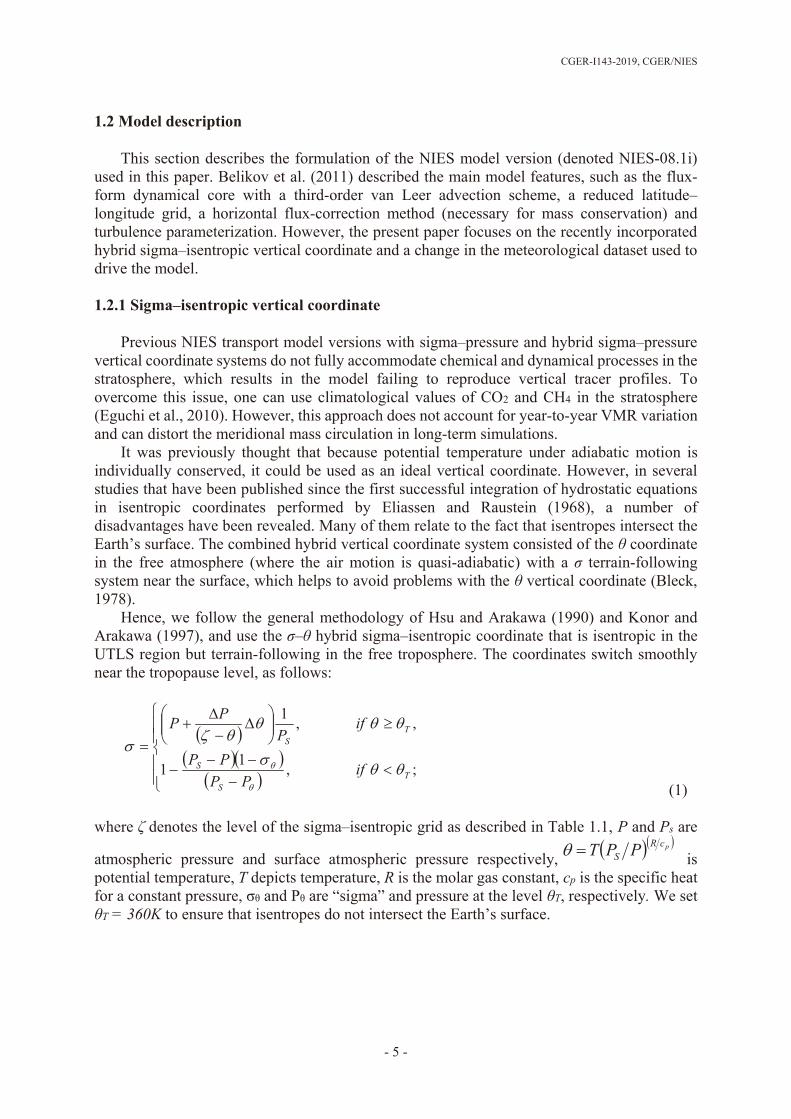
1.2 Model description This section describes the formulation of the NIES model version (denoted NIES-08.1i)
used in this paper. Belikov et al. (2011) described the main model features, such as the flux-form dynamical core with a third-order van Leer advection scheme, a reduced latitude–longitude grid, a horizontal flux-correction method (necessary for mass conservation) and turbulence parameterization. However, the present paper focuses on the recently incorporated hybrid sigma–isentropic vertical coordinate and a change in the meteorological dataset used to drive the model.
1.2.1 Sigma–isentropic vertical coordinate
Previous NIES transport model versions with sigma–pressure and hybrid sigma–pressure
vertical coordinate systems do not fully accommodate chemical and dynamical processes in the stratosphere, which results in the model failing to reproduce vertical tracer profiles. To overcome this issue, one can use climatological values of CO2 and CH4 in the stratosphere (Eguchi et al., 2010). However, this approach does not account for year-to-year VMR variation and can distort the meridional mass circulation in long-term simulations.
It was previously thought that because potential temperature under adiabatic motion is individually conserved, it could be used as an ideal vertical coordinate. However, in several studies that have been published since the first successful integration of hydrostatic equations in isentropic coordinates performed by Eliassen and Raustein (1968), a number of disadvantages have been revealed. Many of them relate to the fact that isentropes intersect the Earth’s surface. The combined hybrid vertical coordinate system consisted of the θ coordinate in the free atmosphere (where the air motion is quasi-adiabatic) with a σ terrain-following system near the surface, which helps to avoid problems with the θ vertical coordinate (Bleck, 1978).
Hence, we follow the general methodology of Hsu and Arakawa (1990) and Konor and Arakawa (1997), and use the σ–θ hybrid sigma–isentropic coordinate that is isentropic in the UTLS region but terrain-following in the free troposphere. The coordinates switch smoothly near the tropopause level, as follows:
;,11
,,1
TS
S
TS
ifPP
PP
ifP
PP
(1)
where ζ denotes the level of the sigma–isentropic grid as described in Table 1.1, P and Ps are
atmospheric pressure and surface atmospheric pressure respectively, pcRS PPT is
potential temperature, T depicts temperature, R is the molar gas constant, cp is the specific heat for a constant pressure, σθ and Pθ are “sigma” and pressure at the level θT, respectively. We set θT = 360K to ensure that isentropes do not intersect the Earth’s surface.
- 5 -

Chapter 1 Simulations of column-averaged CO2 and CH4 using the NIES TM with a hybrid sigma-isentropic (sigma-theta) vertical coordinate
- 6 -
Table 1.1 Levels of the vertical grid in the NIES TM model.
H, km σ =P/Ps ≈Δ, m ζ (σ–θ grid levels), K Number
of levels
Near-surface
layer 0-2 1.0–0.795 250 - 8
Free
troposphere 2–12
0.795–
0.195 1000
-
330, 350 10
Upper
troposphere and
stratosphere
12–40 0.195–
0.003
1000 365, 380, 400, 415,
435, 455, 475, 500
14 2000 545,
– 590, 665, 850,
1325, 1710
Total levels: 32
1.2.2 Simulation of upward motion in the stratosphere
To calculate vertical transport in the θ-coordinate domain of the hybrid sigma–isentropic
coordinate, we use precalculated heating rates. Unlike the SLIMCAT model, which has an embedded diagnostic radiation scheme to calculate heating rates (Chipperfield, 2006), the NIES model interpolates the climatological heating rate at every meteorology data update step (3h) at every model cell of the sigma–isentropic grid using a 2D monthly distribution of the atmospheric reanalysis heating rate (see Section 1.2.3).
The most problematic region in modelling vertical transport is a level around the tropopause transition region known as the Tropical Tropopause Layer (TTL). Radiative heating in the TTL is a result of heating from the absorption of infrared radiation by ozone and carbon dioxide, balanced by infrared cooling, mainly from water vapor (Thuburn and Craig, 2002). The level termed as the ‘stagnation surface’ (Sherwood and Dessler, 2003) occurs where the total heating rate Qtotal = 0, and is demarcated by net cooling below and net heating above. The height of this transition level is almost constantly around θ = 360 K (≈15 km, 125 hPa) (Gettelman et al., 2004; Folkins et al., 1999). There is some variability in the level of Qtotal = 0; e.g., ±500 m between different locations and seasons; ±400 m for individual profiles (Gettelman et al., 2004).
Among other aspects of Troposphere-to-Stratosphere Transport (TST) that are not adequately addressed, it is unclear how air parcels overcome the vertical gap between the main convective outow around 350 K and the level with significant heating rates (Konopka et al., 2007). In some models, erroneous spurious meteorology, a diffusive numerical scheme (Eluszkiewicz et al., 2000), or extra vertical motion due to the implementation of vertical transport misrepresenting the adiabatic conditions are responsible for extra artificial mixing in this region, thereby obscuring the vertical transport problem.
In isentropic coordinates, the impact of such erroneous effects is significantly reduced. As
- 6 -

CGER-I143-2019, CGER/NIES
- 7 -
a result, the use of a simulated heating rate leads to insufficient TST of tracers through the TTL. When models are unable to resolve a process explicitly, it is necessary to implement a parameterization to improve the simulation. Thus, Konopka et al. (2007) showed that more realistic tracer distributions are obtained by implementing the mixing parameterisation into a Chemical Lagrangian Model of the Stratosphere (CLaMS) with an isentropic vertical coordinate. Induced vertical mixing, driven mainly by vertical shear in the tropical flanks of subtropical jets, has been cited in explaining the upward transport of trace species from the main convective outflow to the tropical tropopause around 380 K (Konopka et al., 2007).
The total diabatic heating rates of different reanalysis products can produce dissimilar results (Fueglistaler et al., 2009). In our work, we implemented a scheme with additional transport in the TTL by increasing the air-ascending rate in the TTL, which was adjusted to fit the observed age of air in the stratosphere, as follows:
For levels above 360 K (isentropic part of the vertical coordinate), the air-ascending rate was multiplied by 2.5.
Constant vertical wind component (0.6 K/day) was set at the levels 180–40 hPa for tropical areas (15°S–15°N).
1.2.3 Meteorological data and vertical resolution
NIES TM is an off-line model driven by Japanese reanalysis data covering more than 30
years from 1 January 1979 (Onogi et al., 2007). The period of 1979–2004 is covered by the Japanese 25-year Reanalysis (JRA-25), which is a product of the Japan Meteorological Agency (JMA) and the Central Research Institute of Electric Power Industry (CRIEPI). After 2005, a real-time operational analysis, employing the same assimilation system as JRA-25, has been continued as the JMA Climate Data Assimilation System (JCDAS). The JRA-25/JCDAS dataset is distributed on Gaussian horizontal grid T106 (320 160) with 40 hybrid σ–p levels. The 6-hourly time step of JRA-25/JCDAS is coarser than the 3-hourly data from the National Centers for Environmental Prediction (NCEP) Global Forecast System (GFS) and Global Point Value (GPV) datasets, which were used in the previous model version (Belikov et al., 2011). However, with a better vertical resolution (40 levels on a hybrid σ–p grid versus 25 and 21 pressure levels for GFS and GPV, respectively) it is possible to implement a vertical grid with 32 levels (versus 25 levels used before), resulting in a more detailed resolution of the boundary layer and UTLS region (Table 1.1).
The 2D monthly distribution of the climatological heating rate used to calculate vertical transport in the θ-coordinate domain of the hybrid sigma–isentropic coordinate is prepared from JRA-25 reanalysis data, which are provided as the sum of short- and long-wave components on pressure levels.
1.2.4 Turbulent diffusion and deep convection parameterization
The calculation of turbulent diffusion is similar to that described by Maksyutov et al. (2008).
To separate the transport processes in the well-mixed near-surface layer and free troposphere, we used 3-hourly PBL height data taken from European Centre for Medium-Range Weather Forecasts (ECMWF) Interim Re-Analysis. Above the top of the PBL, the parameterisation of the turbulent diffusivity follows the approach used by Hack et al. (1993), who estimated free-troposphere diffusivity from local stability as a function of the Richardson number. Below the top of the PBL, the turbulent diffusivity is set to a constant value of 40 m2s–1, under the
- 7 -
Chapter 1 Simulations of column-averaged CO2 and CH4 using the NIES TM with a hybrid sigma-isentropic (sigma-theta) vertical coordinate
- 8 -
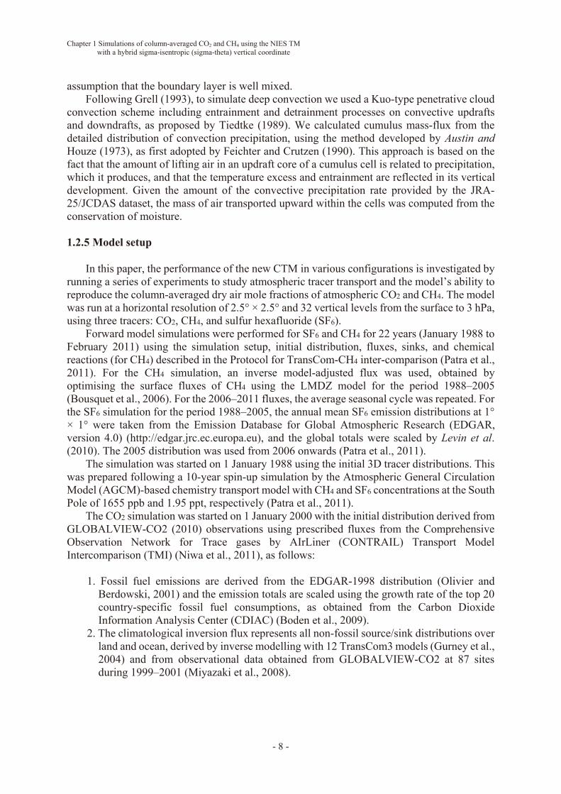
assumption that the boundary layer is well mixed. Following Grell (1993), to simulate deep convection we used a Kuo-type penetrative cloud
convection scheme including entrainment and detrainment processes on convective updrafts and downdrafts, as proposed by Tiedtke (1989). We calculated cumulus mass-flux from the detailed distribution of convection precipitation, using the method developed by Austin and Houze (1973), as first adopted by Feichter and Crutzen (1990). This approach is based on the fact that the amount of lifting air in an updraft core of a cumulus cell is related to precipitation, which it produces, and that the temperature excess and entrainment are reflected in its vertical development. Given the amount of the convective precipitation rate provided by the JRA-25/JCDAS dataset, the mass of air transported upward within the cells was computed from the conservation of moisture.
1.2.5 Model setup
In this paper, the performance of the new CTM in various configurations is investigated by
running a series of experiments to study atmospheric tracer transport and the model’s ability to reproduce the column-averaged dry air mole fractions of atmospheric CO2 and CH4. The model was run at a horizontal resolution of 2.5° × 2.5° and 32 vertical levels from the surface to 3 hPa, using three tracers: CO2, CH4, and sulfur hexafluoride (SF6).
Forward model simulations were performed for SF6 and CH4 for 22 years (January 1988 to February 2011) using the simulation setup, initial distribution, fluxes, sinks, and chemical reactions (for CH4) described in the Protocol for TransCom-CH4 inter-comparison (Patra et al., 2011). For the CH4 simulation, an inverse model-adjusted flux was used, obtained by optimising the surface fluxes of CH4 using the LMDZ model for the period 1988–2005 (Bousquet et al., 2006). For the 2006–2011 fluxes, the average seasonal cycle was repeated. For the SF6 simulation for the period 1988–2005, the annual mean SF6 emission distributions at 1° × 1° were taken from the Emission Database for Global Atmospheric Research (EDGAR, version 4.0) (http://edgar.jrc.ec.europa.eu), and the global totals were scaled by Levin et al. (2010). The 2005 distribution was used from 2006 onwards (Patra et al., 2011).
The simulation was started on 1 January 1988 using the initial 3D tracer distributions. This was prepared following a 10-year spin-up simulation by the Atmospheric General Circulation Model (AGCM)-based chemistry transport model with CH4 and SF6 concentrations at the South Pole of 1655 ppb and 1.95 ppt, respectively (Patra et al., 2011).
The CO2 simulation was started on 1 January 2000 with the initial distribution derived from GLOBALVIEW-CO2 (2010) observations using prescribed fluxes from the Comprehensive Observation Network for Trace gases by AIrLiner (CONTRAIL) Transport Model Intercomparison (TMI) (Niwa et al., 2011), as follows:
1. Fossil fuel emissions are derived from the EDGAR-1998 distribution (Olivier and Berdowski, 2001) and the emission totals are scaled using the growth rate of the top 20 country-specific fossil fuel consumptions, as obtained from the Carbon Dioxide Information Analysis Center (CDIAC) (Boden et al., 2009).
2. The climatological inversion flux represents all non-fossil source/sink distributions over land and ocean, derived by inverse modelling with 12 TransCom3 models (Gurney et al., 2004) and from observational data obtained from GLOBALVIEW-CO2 at 87 sites during 1999–2001 (Miyazaki et al., 2008).
- 8 -

CGER-I143-2019, CGER/NIES
- 9 -
1.3 Results The current model version has been used in several tracer transport studies and was
evaluated through participation in transport model intercomparisons (Niwa et al., 2011; Patra et al., 2011). The model results of tracer transport simulations show good consistency with observations and other models in the near-surface layer and in the free troposphere. However, the model performance in the UTLS region has not been evaluated in detail.
1.3.1 Validation of the mean age of air in the stratosphere
The mean age of air is purely a transport diagnostic. Modellers are ultimately interested in
accurately simulating the distribution of trace gases that are affected by both transport and photochemistry (Waugh and Hall, 2002). The accurate determination of the chemical constituents that are transported across the tropopause, which are strongly affected by synoptic-scale events and other small-scale mixing processes, is a major challenge for modern CTMs (Hall et al., 1999). In the stratosphere, the vertical transport of substances is very weak due to the almost adiabatic conditions. However, many models are unable to reproduce sufficiently weak transport, especially in the tropical lower stratosphere, because the model grid does not reflect the underlying constraint that the flow is almost isentropic, making the model transport vulnerable to numerical errors (Mahowald et al., 2002). Generally, models tend to have ages of air in the stratosphere that are too young and tend to propagate the signal upward from the troposphere into the lower stratosphere too quickly, especially in the tropics (Hall et al., 1999; Park et al., 1999). By implementing a hybrid sigma–isentropic vertical coordinate, the observed age of air is more accurately determined than when using a model that employs a hybrid pressure grid (Mahowald et al., 2002; Chipperfield, 2006; Monge-Sanz et al., 2007).
The mean age of air can be calculated from measured or modelled tracer concentrations that are conserved and that vary linearly with time (Waugh and Hall, 2002). Among several chemical species that approximately satisfy the criterion of linear variation, CO2 and SF6 are the most reliable compounds with which to derive the mean age, because they are very long-lived species and their annual mean concentrations have been increasing approximately linearly (Conway et al., 1994; Maiss et al., 1996). In spite of uncertainties due to nonlinearity in tropospheric growth rates and the neglect of photochemical processes (Waugh and Hall, 2002), estimates performed with CO2, SF6, and other tracers show rather good agreement.
In this paper, SF6 is simulated to derive the mean age of the air in the upper troposphere and in the lower stratosphere. The model was run for 22 years before the simulation results were analysed, because the age of stratospheric air was unchanged for the last 30 years (Engel et al., 2009).
Figure 1.1 shows the annual mean of the zonal-mean age of air obtained with NIES TM at an altitude of 20 km, together with the mean age values derived from CO2 and SF6 ER-2 aircraft observations (Andrews et al., 2001). Both the model and observation estimations of the mean age indicate values of approximately 1 year near the equator, large gradients in the subtropics, and values of around 4–5 years at high latitudes.
The vertical profiles of mean age derived from in situ measurements of CO2 and SF6 show that at all latitudes, the mean age of the air increased monotonically with height throughout the stratosphere, with only weak vertical gradients above 25 km (Figure 1.2). The model slightly overestimated the age of air in the tropics (Figure 1.2a) and underestimated it at middle and high latitudes (Figure 1.2b, c). The spikes in high-latitude profiles (Figure 1.2c) are due to the sampling of fragments of polar vortex air. Despite this, the general shape of the isopleths in
- 9 -

Chapter 1 Simulations of column-averaged CO2 and CH4 using the NIES TM with a hybrid sigma-isentropic (sigma-theta) vertical coordinate
- 10 -
Figure 1.3 is realistic and illustrates the balance of the meridional mass (Brewer–Dobson) circulation, which tends to increase latitudinal slopes, and isentropic mixing, which tends to decrease the slopes (Plumb and Ko, 1992).
Figure 1.1 Mean age of air at 20 km altitude from NIES TM simulations (blue line), compared
with the mean age of air derived from in situ ER-2 aircraft observations of CO2 (Andrews et al., 2001) and SF6 (Ray et al., 1999) (red line). Error bars for the observations are 2σ (Monge‐Sanz et al., 2007).
Figure 1.2 Comparison of observed and modelled (red lines) mean age of air at latitudes of: (a) 5°S, (b) 40°N, and (c) 65°N. The lines with symbols represent observations: in situ SF6 (dark blue line with triangles) (Elkins et al., 1996; Ray et al., 1999), whole air samples of SF6 (purple line with squares for (b) panel, light blue line with squares outside vortex and orange line with asterisks inside vortex (c) panel) (Harnisch et al., 1996), and mean age from in situ CO2 (green line with diamonds) (Boering et al., 1996; Andrews et al., 2001).
- 10 -

CGER-I143-2019, CGER/NIES
- 11 -
Figure 1.3 Cross-section of the annual mean age of air (years) from NIES TM simulations of SF6 with JRA-25/JCDAS reanalysis.
1.3.2 Validation of CO2, CH4, and SF6 vertical profiles in the stratosphere To evaluate the model’s ability to reproduce stratospheric transport, the simulated vertical
profiles of CO2, CH4, and SF6 were analysed and compared against balloon-borne observation data (Figure 1.4). The observed VMRs were derived from six individual profiles of balloon-borne measurements performed by Prof. Takakiyo Nakazawa and Shuhji Aoki (Tohoku University) for Sanriku, Japan (39.17°N, 141.83°E) for 28 August 2000, 30 May 2001, 4 September 2002, 6 September 2004, 3 June 2006, and 4 June 2007, following the procedures described by Nakazawa et al. (2002). The vertical profiles were determined by averaging the modelled and observed concentrations taken for the same day and time. The error bars show the standard deviation. To calculate the mean profiles, we subtracted the annual growth rate of 0.23 pptv/yr (Stiller et al., 2008) for SF6 and variable growth rates derived by Conway and Tans (2011) for CO2 for the period 2001–2007. No correction is applied to the CH4 concentration, because a slowdown in the CH4 increase was observed in the stratosphere for the period 1978–2003 (Rohs et al., 2006).
In general, the NIES TM is able to capture the shape of a tracer’s vertical profile in the stratosphere. These profiles consist of several parts with different properties, such as: 1) weak gradients up to 70 hPa; 2) a large decrease of VMRs at heights between 70 and 50 hPa; 3) almost constant concentrations from 50 to 30 hPa, and 4) significant (especially for CH4) gradients from 30 hPa upwards (Figure 1.4).
The modelled profile of SF6 is consistent with the observed profile up to 50 hPa and has a relatively large (~5%) positive bias above this level (Figure 1.4a). SF6 is a chemically inert tracer (in the troposphere and stratosphere), indicating that transport alone is responsible for the variation in its profile. The discrepancy between the observed and simulated vertical profiles is consistent with the underestimation of the age of air above 40 hPa in temperate and high-latitude zones, as discussed above.
In contrast, the CH4 profile was found to have a strong negative bias (~5%) between 100 and 20 hPa (Figure 1.4b), which disappeared with height. It would appear that a change in the CH4 loss rate due to chemical reactions leads to less excessive destruction of methane and better agreement with observations above 20 hPa. SF6 is not involved in any chemical reactions to
Figure 1.3 Cross-section of the annual mean age of air (years) from NIES TM simulations of SF6 with JRA-25/JCDAS reanalysis.
- 11 -

Chapter 1 Simulations of column-averaged CO2 and CH4 using the NIES TM with a hybrid sigma-isentropic (sigma-theta) vertical coordinate
- 12 -
compensate for the extra vertical transport in the UTLS region. The simulated CO2 vertical profile (Figure 1.4c) overestimated the observed profile by
0.5% below 90 hPa and underestimated it by 0.5% above 90 hPa. The individual profiles used to derive the average profile were obtained at the beginning and end of the vegetation season; consequently, the modelled CO2 profile shows a seasonal variation at the 140–100 hPa level. The large error bars become smaller with height, enabling an estimate of the seasonal variation of approximately 1–2 ppmv at 140 hPa. The spread of data in the profiles at about 1.5 ppmv at all levels is common for measured CO2.
Figure 1.4 Comparison of observed and modelled concentration averaged for the period 2000–
2007: a) SF6, b) CH4, and c) CO2. The observed VMRs were derived from six individual profiles of balloon-borne measurements over Sanriku, Japan (39.17°N, 141.83°E).
Thus, the simulated vertical profiles of CH4 and SF6 are generally within ∼5% of the observed VMRs, while CO2 profiles are within 1%. Given that the stratosphere only represents 15%–20% of the mid-latitude atmospheric column mass, these results are sufficient for this study. It is noted that the simulated CO2 profiles have a smoother shape and show a better consistency with the observations, as the simulation was run for 9 years less than that for CH4 and SF6. This result indicates the ability of the model to reproduce vertical profiles of the tracers in the lower stratosphere more accurately for a relatively short-term period (about 10 years) than for a long-term period (about 20 years). This result reflects the fact that the model tends to overestimate tracer concentrations in the uppermost part of the domain, due to sparse grid layers in the lower stratosphere. 1.3.3 Validation of CO2, CH4, and SF6 concentrations in the free troposphere
The ability of the NIES TM to simulate SF6 and CO2 in the near-surface layer and in the
free troposphere was validated by Belikov et al. (2011) and Niwa at al. (2011). The inter-hemispheric gradients of SF6 and CO2, and vertical profiles and seasonal variations of CO2 were evaluated against the GLOBALVIEW-CO2 and World Data Centre for Greenhouse Gases (WDCGG) observations, and against an aircraft measurement dataset of CONTRAIL (Niwa at
Figure 1.4 Comparison of observed and modelled concentration averaged for the period 2000–
2007: a) SF6, b) CH4, and c) CO2. The observed VMRs were derived from six individual profiles of balloon-borne measurements over Sanriku, Japan (39.17°N, 141.83°E).
- 12 -
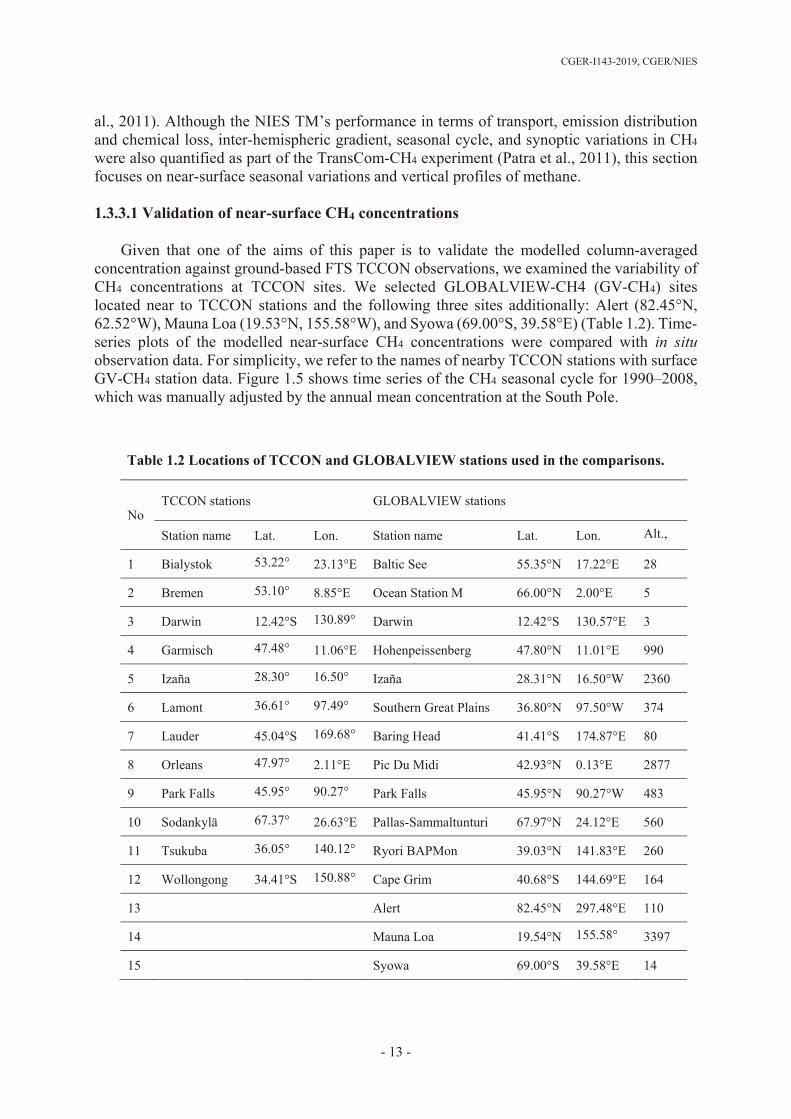
CGER-I143-2019, CGER/NIES
- 13 -
al., 2011). Although the NIES TM’s performance in terms of transport, emission distribution and chemical loss, inter-hemispheric gradient, seasonal cycle, and synoptic variations in CH4 were also quantified as part of the TransCom-CH4 experiment (Patra et al., 2011), this section focuses on near-surface seasonal variations and vertical profiles of methane. 1.3.3.1 Validation of near-surface CH4 concentrations
Given that one of the aims of this paper is to validate the modelled column-averaged
concentration against ground-based FTS TCCON observations, we examined the variability of CH4 concentrations at TCCON sites. We selected GLOBALVIEW-CH4 (GV-CH4) sites located near to TCCON stations and the following three sites additionally: Alert (82.45°N, 62.52°W), Mauna Loa (19.53°N, 155.58°W), and Syowa (69.00°S, 39.58°E) (Table 1.2). Time-series plots of the modelled near-surface CH4 concentrations were compared with in situ observation data. For simplicity, we refer to the names of nearby TCCON stations with surface GV-CH4 station data. Figure 1.5 shows time series of the CH4 seasonal cycle for 1990–2008, which was manually adjusted by the annual mean concentration at the South Pole.
Table 1.2 Locations of TCCON and GLOBALVIEW stations used in the comparisons.
No TCCON stations GLOBALVIEW stations
Station name Lat. Lon. Station name Lat. Lon. Alt.,
1 Bialystok 53.22° 23.13°E Baltic See 55.35°N 17.22°E 28
2 Bremen 53.10° 8.85°E Ocean Station M 66.00°N 2.00°E 5
3 Darwin 12.42°S 130.89° Darwin 12.42°S 130.57°E 3
4 Garmisch 47.48° 11.06°E Hohenpeissenberg 47.80°N 11.01°E 990
5 Izaña 28.30° 16.50° Izaña 28.31°N 16.50°W 2360
6 Lamont 36.61° 97.49° Southern Great Plains 36.80°N 97.50°W 374
7 Lauder 45.04°S 169.68° Baring Head 41.41°S 174.87°E 80
8 Orleans 47.97° 2.11°E Pic Du Midi 42.93°N 0.13°E 2877
9 Park Falls 45.95° 90.27° Park Falls 45.95°N 90.27°W 483
10 Sodankylä 67.37° 26.63°E Pallas-Sammaltunturi 67.97°N 24.12°E 560
11 Tsukuba 36.05° 140.12° Ryori BAPMon 39.03°N 141.83°E 260
12 Wollongong 34.41°S 150.88° Cape Grim 40.68°S 144.69°E 164
13 Alert 82.45°N 297.48°E 110
14 Mauna Loa 19.54°N 155.58° 3397
15 Syowa 69.00°S 39.58°E 14
- 13 -

Chapter 1 Simulations of column-averaged CO2 and CH4 using the NIES TM with a hybrid sigma-isentropic (sigma-theta) vertical coordinate
- 14 -
Figure 1.5 Detrended seasonal cycle of surface CH4 volume mixing ratio for GLOBALVIEW
stations (corresponding TCCON stations in parentheses): a) Baltik See (Bialystok); b) Ocean Station M (Bremen); c) Darwin (Darwin); d) Hohenpeissenberg (Garmisch); e) Izaña (Izaña); f) Southern Great Plains (Lamont); g) Baring Head Station (Lauder); h) Pic Du Midi (Orleans).
- 14 -

CGER-I143-2019, CGER/NIES
- 15 -
Figure 1.5 (Continued) Detrended seasonal cycle of surface CH4 volume mixing ratio for GLOBALVIEW stations (corresponding TCCON stations in parentheses): i) Park Falls (Park Falls); j) Pallas-Sammaltunturi (Sodankylä); k) Ryori (Tsukuba); l) Cape.Grim (Wollongong); m) Alert; n) Mauna Loa; and o) Syowa.
The simulations indicate that the model underestimated the near-surface seasonal cycle at northern high-latitudes. The model bias for Alert was 13.0 ppb versus 8.4 and 6.5 ppb for Mauna Loa and Syowa, respectively. A similar feature was observed for the trend of CH4, for which the model bias decreased from the North Pole (0.5 ppb/yr) to the South Pole (0.1 ppb/yr) (Figure 1.6).
Southern Australia and New Zealand are relatively isolated from large-scale CH4 emission sources, and as a result there was some consistency between the modelled and measured values
- 15 -

Chapter 1 Simulations of column-averaged CO2 and CH4 using the NIES TM with a hybrid sigma-isentropic (sigma-theta) vertical coordinate
- 16 -
(r = 0.87–0.9 for Baring Head and Cape Grim) in capturing the small variability (amplitude of 30 ppb). As Darwin is located relatively close to the Asian tropics (Malaysia and Indonesia), which is marked by very high variations in CH4 emissions and complicated meteorological conditions, the model was not able to reproduce the seasonal cycle as well at this site, compared with other sites.
The results for North America, whilst including a range of emission sources, indicated a similar agreement in the phase for Park Falls and Southern Great Plains (Lamont) (r ~ 0.7) and performed poorly in reproducing the growth rate, as the model underestimated the trends for both sites (Figure 1.6). Mixed results were also found for the European sites: good agreement with observations was found for Pic Du Midi (Orleans) and Ocean Station M (Bremen), but poor agreement for Hohenpiessenberg (Garmisch) and Pallas-Sammaltunturi (Sodankylä). However, the worst agreement in the growth rate was found for Ryori (Tsukuba), where the model systematically underestimated the seasonal variations of the tracer.
Figure 1.6 Average difference between simulated and observed trends (ppb/yr) of CH4 for Jan 1990 and Dec 2009 at GLOBALVIEW stations.
We found very different model performance at remote sites such as Ocean Station M (Bremen), Izaña, Cape Grim (Wollongong), Baring Head (Lauder), Alert, Mauna Loa, and Syowa, where the model was generally able to accurately reproduce the phase of variations in surface concentrations (correlation coefficients of 0.85–0.95) (Figure 1.7). For other sites (Park Falls, Pallas-Sammaltunturi (Sodankylä), Ryori (Tsukuba), and Southern Great Plains (Lamont)), however, where multiple emission sources are located close by and where local meteorology plays a major role, the model encountered difficulties in reproducing the complicated CH4 surface concentrations.
- 16 -

CGER-I143-2019, CGER/NIES
- 17 -
Figure 1.7 Correlation coefficients between simulated and observed CH4 at GLOBALVIEW stations.
1.3.3.2. Validation of CH4 vertical profiles in the troposphere
To examine the variability of CH4 in the near-surface layer and in the free troposphere, the
VMRs simulated by the model were compared against aircraft observations performed by T. Machida (NIES) in 1993–2007 over Surgut, West Siberia. This location is marked by high CH4 emissions from wetlands.
It is challenging to perform simulations of CH4 in the northern high-latitude regions because of large uncertainties in emissions due to under-sampling of CH4 concentrations over most regions, particularly where melting permafrost releases CH4 (Zhuang et al., 2009). Despite this problem, the modelled and measured values are in good agreement above 1 km (Figure 1.8). The model is less effective in reproducing the high variability in CH4 concentrations in the near-surface layer and could not accurately simulate short-term variations. The VMR at the 1-km level and below was highly variable due to changes in the PBL height, which determined the volume of air absorbing all emitted tracers and the local meteorology. The greatest amount of variability was found in July and August (Figure 1.8), reflecting variations in the PBL height during the daytime and high emissions from wetlands.
Figure 1.7 Correlation coefficients between simulated and observed CH4 at GLOBALVIEW stations.
- 17 -

Chapter 1 Simulations of column-averaged CO2 and CH4 using the NIES TM with a hybrid sigma-isentropic (sigma-theta) vertical coordinate
- 18 -
Figure 1.8 Comparison of observed and modeled CH4 concentrations averaged for the period 1993-2007 over Surgut, West Siberia. The vertical profiles were produced by averaging the modelled and observed concentrations taken on the same day and at the same time. Error bars show the standard deviation.
The averaged trends derived from the biases for the levels at 1, 3, and 7 km show similar values in all cases, in the range about 40 ppb depending on the season (Figure 1.9). This result indicates balanced transport from the surface layer to the free troposphere due to the implementation of the JR-25/JCDAS meteorological data provided on the sigma–pressure levels.
Figure 1.8 Comparison of observed and modeled CH4 concentrations averaged for the period 1993-2007 over Surgut, West Siberia. The vertical profiles were produced by averaging the modelled and observed concentrations taken on the same day and at the same time. Error bars show the standard deviation.
- 18 -

CGER-I143-2019, CGER/NIES
- 19 -
Figure 1.9 Time series of model bias (modelled CH4 concentration minus observed) and the averaged (moving average with period 12) value of the bias for the 1, 3, and 7 km levels over Surgut (61.25°N, 73.43°E) for the period 1993–2007.
The correlation coefficients between simulated and observed CH4 values show an increase towards the free troposphere, from 0.19 for the 1-km level to 0.53 for the 7-km level, because vertical propagation decreases with height. While other factors are involved, changes in PBL height and associated variation in the rates of tracer redistribution from local sources to the free troposphere are important drivers of high variability in CH4 VMR at GV-CH4 sites with high emissions. Similar trends were obtained by Houweling et al. (2010) for four different transport models used to simulate XCO2. 1.3.4 Validation of CO2 and CH4 column-averaged DMFs
The main goal of this paper was to validate the model’s ability to reproduce the CO2 and
CH4 column-averaged dry-air mole fractions using observations from TCCON sites, which is a global network of ground-based high-resolution FTS recording direct solar spectra in the near-infrared spectral region (Wunch et al., 2011). The overall objectives of TCCON include improving our understanding of the carbon cycle and validating XCO2 and XCH4 retrieved from satellite observations.
For comparison, we selected simulated and TCCON measured concentrations of XCO2 and XCH4 taken at around 13:00 ± 1 hour local time over TCCON sites for the period January 2009 to January 2011. Samples within this time-frame were collected for analysis, to assess the model’s performance within the GOSAT overpass interval. The following the TCCON sites were selected: Bialystok (Poland, 53.22°N, 23.13°E); Bremen (Germany, 53.10°N, 8.85°E); Darwin (Australia, 12.42°S, 130.89°E); Garmisch (Germany, 47.48°N, 11.06°E); Izaña (Spain, 28.30°N, 16.50°W); Lamont (USA, 36.6°N, 97.49°W); Lauder (New Zealand, 45.04°S, 169.68°E); Orleans (France, 47.97°N, 2.11°E); Park Falls (USA, 45.95°N, 90.27°W); Sodankylä (Finland, 67.37°N, 26.63°E); Tsukuba (Japan, 36.05°N, 140.12°E); and Wollongong (Australia, 34.41°S, 150.88°E). For the Lauder site we used data from the 125HR spectrometer when available (February 2010-present) and data from the older 120HR spectrometer prior to February 2010.
To compare the modelled total column with measurements directly, it is necessary to
- 19 -

Chapter 1 Simulations of column-averaged CO2 and CH4 using the NIES TM with a hybrid sigma-isentropic (sigma-theta) vertical coordinate
- 20 -
consider the measurement averaging kernels. Averaging kernels describe the sensitivity of the retrieved total column to a perturbation in absorber abundance in a given layer of the vertical profile (Rodgers and Connor, 2003; Wunch et al., 2011). At present TCCON provides a single set of averaging kernels for CO2 and CH4, tabulated as a function of solar zenith angle (SZA), based on a subset of retrievals from the Lamont site (http://tccon.ipac.caltech.edu/tccon_aux_pub.html). Site-specific a priori profiles used in TCCON CO2 retrievals were provided by each site PI (http://tccon.ipac.caltech.edu/tccon_aux_pub.html). A single CH4 a priori (independent of location and time) has been used in TCCON retrievals at all sites other than Darwin and Sodankylä. At these sites site-specific and time-independent CH4 profiles are provided. The tabulated averaging kernels were interpolated to the SZA of the measurements and applied in the calculation of the CO2 or CH4 vertical column in accordance with Equation 15 of Connor et al. (2008). The tracer vertical column abundances were then divided by the dry-air column abundance to calculate the column-averaged dry air mole fractions, denoted Xy or DMF hereafter.
Due to the SZA dependence of the TCCON averaging kernels, the difference between total column concentrations calculated with and without averaging kernels is greatest for sites located farthest from the equator, Bialystok, Bremen and Sodankylä, which yield values in the range –0.6 to 2.0 ppm and –20 to 20 ppb for XCO2 and XCH4, respectively; the difference is smallest for the tropical and subtropical sites Darwin and Izaña, with values of –0.4 to 0.4 ppm and –5.0 to 5.0 ppb, respectively.
Time series of the model results and FTS data for XCO2 and XCH4 are shown in Figures 10 and 12, respectively. These figures were produced by manually adjusting the XCO2 and XCH4 model offsets (2.2 ppm and –32.0 ppb, respectively). The offsets were caused by the use of slightly out-dated fluxes for the simulations, the implementation of an averaging kernel, and misfit in the modelled vertical profiles. Thus, a XCH4 offset may also be induced due to high uncertainty of OH and other species, which are responsible for CH4 destruction in the atmosphere.
Matching the model’s mean CH4 with the observations is achieved by adjusting either global total emissions or sinks, which both have large uncertainties (10-20%, Patra et al., 2011). Small residual offsets can be adjusted by tuning global emissions, but long-term simulations are required to reach equilibration between sources and sinks. Adding a small 30 ppb offset to simulated results is nearly equivalent to the corresponding proportional change in the emissions fields on the order of 2%. For CO2, the corresponding bias correction is about 0.5%.
For TCCON, the observation symbols and error bars represent the mean and standard deviations of the weighted average if more than one measurement within the 13:00 ± 1 hour local time was available. Note that gaps in the TCCON data time-series are due to cloud and instrumental issues. 1.3.4.1 Modelled XCH4 compared with TCCON FTS observations
Reproducing the CH4 seasonal variation was a big challenge, because of its rather small amplitude and high scatter relative to the mean climatological value. As expected, the seasonal variation in XCH4 over the Southern Hemisphere (i.e., Darwin, Lauder, and Wollongong) was weak (Figure 1.10a, g, h) due to the smaller contribution of the local emissions; consequently, the model’s ability to reproduce the variation generally depends on reproducing of large-scale transport. The correlation coefficients for these sites are very similar (0.55, 0.58, and 0.66, respectively; Table 1.3).
- 20 -

CGER-I143-2019, CGER/NIES
- 21 -
In contrast, model performance at the Northern sites strongly depends on powerful local sources. The best correlation coefficients (in the range of 0.62-0.74) are obtained for Lamont, Bremen and Bialystok, where seasonal variation in XCH4 has the highest amplitude. European sites show slightly large biases of 4.52, -8.80, and 20.91 for Bialystok, Orleans and Sodankylä, respectively. For Orleans, the correlation is rather weak (0.59, Table 1.3), whereas for the corresponding GlobalView station of Pic Du Midi it is rather strong (>0.85, Figure 1.7). This is due to the fact that Pic Du Midi is a high altitude site (free troposphere) and Orleans a lowland site affected by near-surface small scale processes.
For Sodankylä, the comparison with the FTS data shows a relatively large bias (b=20.91 ppb) and low correlation coefficient (r = 0.40), with larger mismatch in April. The bias may be caused by a overestimation of modelled CH4 inside the polar vortex. Inside the vortex, the descent is much faster than in the zonal average and the stratospheric air with low concentrations of CH4 drops to the troposphere. The ability of NIES TM to reproduce the observations in the vicinity of the polar vortex is also limited due horizontal grid resolution and a horizontal flux correction method implemented to NIES TM (Belikov et al., 2011). “Noise” appearing through the horizontal mass flux correction method may affect the vertical component of the wind vector and cause erroneously enhanced mixing and mass transport from the bottom of the atmosphere to the top (Belikov et al., 2011). In addition, NIES TM underestimates the age of air at high latitudes (Figure 1.3c).
For Wollongong, the simulated results strongly underestimated the measurements (bias -11.05ppb), as the FTS’ seasonal cycle amplitude was twice (Figure 1.10l) the model value and twice that for other TCCON sites in the Southern Hemisphere. The reasons for this result remain unclear, although it may be relevant that Wollongong is located near major urban centers and sites of industrial activity, where emissions from coal mining are the largest source above background (Fraser et al., 2011).
The Izaña TCCON station is an oceanic site located on a small island and at high altitude (~2km). The model’s grid is too rough to reproduce local emission and loss, or capture the topography. The model is not able to reproduce small-scale variations in concentration, and this results in a weak correlation (0.53) and large bias (9.05 ppb).
In general, the minimum and maximum bias between the two datasets is –8.80 ppb (–0.49 %) and 20.91 ppb (1.16 %), respectively. Figure 1.11 shows a scatter diagram of model XCH4 data versus ground-based FTS XCH4 data for 12 sites. The majority of points are within an interval of ±1% of XCH4
- 21 -

Chapter 1 Simulations of column-averaged CO2 and CH4 using the NIES TM with a hybrid sigma-isentropic (sigma-theta) vertical coordinate
- 22 -
Figure 1.10 Time series of XCH4 measured by FTS and modelled by NIES TM for the period
January 2009 to February 2011, for the following stations: a) Bialystok (Poland, 53.22°N, 23.13°E); b) Bremen (Germany, 53.10°N, 8.85°E); c) Darwin (Australia, 12.42°S, 130.89°E); d) Garmisch (Germany, 47.48°N, 11.06°E); e) Izaña (Spain, 28.30°N, 16.50°W); f) Lamont (USA, 36.6°N, 97.49°W). The “error” for each symbol is a combination of the spread due to weighted averaging within the 13:00 ± 1 hour local time interval and observation error.
- 22 -

CGER-I143-2019, CGER/NIES
- 23 -
Figure 1.10 (Continued) Time series of XCH4 measured by FTS and modelled by NIES TM for the period January 2009 to February 2011, for the following stations: g) Lauder (New Zealand, 45.04°S, 169.68°E); h) Orleans (France, 47.97°N, 2.11°E); i) Park Falls (USA, 45.95°N, 90.27°W); j) Sodankylä (Finland, 67.37°N, 26.63°E); k) Tsukuba (Japan, 36.05°N, 140.12°E); and l) Wollongong (Australia, 34.41°S, 150.88°E). The “error” for each symbol is a combination of the spread due to weighted averaging within the 13:00 ± 1 hour local time interval and observation error.
Figure 1.10 (Continued) Time series of XCH4 measured by FTS and modelled by NIES TM for the period January 2009 to February 2011, for the following stations: g) Lauder (New Zealand, 45.04°S, 169.68°E); h) Orleans (France, 47.97°N, 2.11°E); i) Park Falls (USA, 45.95°N, 90.27°W); j) Sodankylä (Finland, 67.37°N, 26.63°E); k) Tsukuba (Japan, 36.05°N, 140.12°E); and l) Wollongong (Australia, 34.41°S, 150.88°E). The “error” for each symbol is a combination of the spread due to weighted averaging within the 13:00 ± 1 hour local time interval and observation error.
- 23 -

Chapter 1 Simulations of column-averaged CO2 and CH4 using the NIES TM with a hybrid sigma-isentropic (sigma-theta) vertical coordinate
- 24 -
Table 1.3 Correlation coefficients and biases of the modelled XCO2 and XCH4.
N Station name XCO2 XCH4
Correlation Bias, ppm Correlation Bias, ppb
1 Bialystok (Poland, 53.22°N, 23.13°E) 0.93 0.61 0.74 4.52
2 Bremen (Germany, 53.10°N, 8.85°E) 0.88 0.19 0.72 1.27
3 Darwin (Australia, 12.42°S, 130.89°E) 0.90 -0.62 0.55 -2.41
4 Garmisch (Germany, 47.48°N, 11.06°E) 0.93 0.76 0.44 0.98
5 Izaña (Spain, 28.30°N, 16.50°W) 0.87 -0.53 0.53 9.05
6 Lamont (USA, 36.61°N, 97.49°W) 0.91 -0.44 0.62 -1.13
7 Lauder (New Zealand, 45.04°S, 169.68°E) 0.90 0.22 0.58 -1.20
8 Orleans (France, 47.97°N, 2.11°E), 0.96 0.17 0.59 -8.80
9 ParkFalls (USA, 45.95°N, 90.27°W) 0.95 -0.28 0.51 -2.30
10 Sodankylä (Finland, 67.37°N, 26.63°E) 0.94 1.21 0.40 20.91
11 Tsukuba (Japan, 36.05°N, 140.12°E) 0.85 -0.24 0.53 3.80
12 Wollongong (Australia, 34.41°S, 0.80 0.32 0.66 -8.19
All stations 0.90 -0.62 (-0.16%)
1.21 (0.31%) 0.54
-8.80 (-0.49%)
20.91 (1.16%)
Figure 1.11 Scatter diagram of modelled and FTS XCH4 at all FTS sites. Dotted lines show a standard deviation of ±1% of XCH4.
Figure 1.11 Scatter diagram of modelled and FTS XCH4 at all FTS sites. Dotted lines show a standard deviation of ±1% of XCH4.
- 24 -

CGER-I143-2019, CGER/NIES
- 25 -
1.3.4.2 Modelled XCO2 compared with TCCON FTS observations and GECM We compared XCO2 time-series with TCCON and constructed a 3-D CO2 climatology
GECM (Gap-filled and Ensemble Climatology Mean) (Saito et al., 2011) (Figure 1.12.). The seasonally varying climatology in GECM was estimated by taking an ensemble of the various transport models in combination with the interpolated bias correction, using a data product based on in situ measurements in the troposphere (GLOBALVIEW-CO2, 2010) and the monthly vertical and latitudinal distribution of the ACTM-derived mean age of air in the stratosphere. Six transport models (ACTM, LMDZ4, NICAM, PCTM, and TM5), including the previous version of NIES TM (Belikov et al., 2011), participated in this study, but this is considered unlikely to seriously distort the results. The GECM seasonal cycle was nudged towards a seasonal cycle of the extended CO2 record (GLOBALVIEW-CO2, 2010) by filtering out the inter-annual anomalies and the synoptic-scale variability in the extended CO2 records using a curve-fitting procedure (Masarie and Tans, 1995).
The modelled XCO2 and GECM XCO2 time series show strong correlations with the TCCON data (correlation coefficients of 0.8–0.9; Table 1.3), as the seasonal XCO2 variation is stronger than the XCH4 cycle. Because of the use of actual meteorology and more up-to-date fluxes, the NIES TM described the seasonal variations slightly better for Bialystok, Bremen, Darwin, Lamont, Lauder, and Wollongong. Moreover, for all sites except Park Falls, Tsukuba, and Wollongong, the model bias was less than the bias for GECM. At other sites, comparisons of the model versus FTS and GECM versus FTS produced almost identical results.
The model shows quite good results in reproducing different seasonal cycles for all considered sites, including very steep decrease of XCO2 at Sodankylä during the growing season and almost flat profiles at sites in the Southern Hemisphere. Figure 1.13 shows a scatter diagram of model XCO2 data versus ground-based FTS XCO2 data. The minimum and maximum differences in the model data compared with the FTS data are -0.62 ppm (-0.16 %) and 1.21 ppm (0.31 %), respectively.
For XCO2 there are several events with only one FTS measurement taken at approximately 13:00 ± 1 hour local time. Generally, the standard error in such cases is quite large especially for Lamont and Tsukuba (Figure 1.12.f, k).
- 25 -

Chapter 1 Simulations of column-averaged CO2 and CH4 using the NIES TM with a hybrid sigma-isentropic (sigma-theta) vertical coordinate
- 26 -
Figure 1.12 Time series of XCO2 measured by FTS, modelled by NIES TM and derived from a 3-D CO2 climatology GECM for the period January 2009 to February 2011, for the following stations: a) Bialystok (Poland, 53.22°N, 23.13°E); b) Bremen (Germany, 53.10°N, 8.85°E); c) Darwin (Australia, 12.42°S, 130.89°E); d) Garmisch (Germany, 47.48°N, 11.06°E); e) Izaña (Spain, 28.30°N, 16.50°W); f) Lamont (USA, 36.6°N, 97.49°W). The “error” for each symbol is a combination of the spread due to weighted averaging within the 13:00 ± 1 hour local time interval and observation error.
- 26 -

CGER-I143-2019, CGER/NIES
- 27 -
Figure 1.12 (Continued) Time series of XCO2 measured by FTS, modelled by NIES TM and derived from a 3-D CO2 climatology GECM for the period January 2009 to February 2011, for the following stations: g) Lauder (New Zealand, 45.04°S, 169.68°E); h) Orleans (France, 47.97°N, 2.11°E); i) Park Falls (USA, 45.95°N, 90.27°W); j) Sodankylä (Finland, 67.37°N, 26.63°E); k) Tsukuba (Japan, 36.05°N, 140.12°E); and l) Wollongong (Australia, 34.41°S, 150.88°E). The “error” for each symbol is a combination of the spread due to weighted averaging within the 13:00 ± 1 hour local time interval and observation error.
1.4 Discussion
The model was able to reproduce the seasonal and inter-annual variability of XCO2 and XCH4 with correlation coefficients of 0.8–0.9 and 0.4–0.7, respectively. A small correlation was obtained for methane, due to the weak seasonal cycle of CH4 and a high scatter of XCH4 obtained from the ground FTS data within the selected interval (13:00 ± 1 hour local time). The modelled time-series have quite small biases for all sites excluding Sodankylä, where model shows a large bias both for XCO2 and XCH4, 1.21 ppm and 20.91 ppb, respectively. Moreover, GECM results also show a large bias (1.22 ppm) for this site. Without Sodankylä’s data, the
- 27 -

Chapter 1 Simulations of column-averaged CO2 and CH4 using the NIES TM with a hybrid sigma-isentropic (sigma-theta) vertical coordinate
- 28 -
model bias is ±0.2% and ±0.5% for XCO2 and XCH4, respectively. Model overestimation of CO2 and CH4 in the troposphere over Sodankylä during spring
2010 likely to be caused by errors in reproducing the polar vortex and requires further improvements in model parameterizations. Comparison with the other model simulations suggests the issue is not unique for NIES TM and difficult to attribute just to the use of average descent/cooling rates to calculate vertical transport in the stratosphere, as for example the online ACTM model with frequent update of the radiative transport has also been shown to possess large biases between the observed and modeled XCH4 (Saito at al., 2012).
The tracer column-averaged dry-air mole fraction is a sensitive indicator of overall model performance, because it is relatively unaffected by changes in vertical transport and surface pressure, and shows minor spatial and temporal variations. As a result, the total column represents the model performance on a global scale. The XCO2 and especially the XCH4 scatter diagrams (Figures 11 and 13, respectively) show balanced redistributions of tracer concentrations from the Northern Hemisphere, with high emissions to the Southern Hemisphere reproduced by the model. Moreover, the Darwin site shows vertical redistribution due to powerful tracer outflow from the PBL into the troposphere and the stratosphere, because this site is located in the tropics. The good agreement between simulated XCH4 and FTS measurements highlights the ability of the model to capture the vertical profile of tracers, and in particular, to simulate balanced transport across the tropopause, as the mean age of methane was markedly different in the lower stratosphere and upper troposphere. 1.5 Conclusions
We performed multi-annual simulations of CO2, CH4, and SF6 using the NIES three-dimensional offline chemical transport model (version NIES-08.1i), driven by JRA-25/JCDAS reanalysis data. This version uses a flexible hybrid sigma–isentropic (σ–θ) vertical coordinate consisting of terrain-following and isentropic levels switched smoothly near the tropopause. Vertical transport in the isentropic part of the grid in the stratosphere was controlled by an air-ascending rate derived from the effective heating rate from JRA-25/JCDAS reanalysis, and was adjusted to fit the observed age of air in the stratosphere. The use of this vertical transport scheme avoided spurious vertical mixing caused by interpolation of the meteorological vertical wind component, and this resulted in improved model performance in the stratosphere, as the simulated vertical profiles of CO2, CH4, and SF6 showed good agreement with balloon-borne observations. A comparison of model data with balloon-borne observations over Sanriku (Japan) in 2000–2007 revealed that the tracer transport simulations were performed with accuracies of ∼5% for CH4 and SF6, and ∼1% for CO2 compared with the observed VMRs.
We evaluated the model performance in simulating near-surface CH4 concentrations by comparisons with measurements at GLOBALVIEW-CH4 sites. In general, the model was able to reproduce the variations in the surface concentrations more accurately (r = 0.6–0.8) at sites located some distance away from multiple emission sources. For other sites, where high emissions and local meteorology play a major role, it proved difficult to reproduce the CH4 surface concentrations.
For measurements above 1 km, the model data are in good agreement with aircraft observations (1993–2007) over Surgut, West Siberia, which is an area with high emissions of methane from wetlands. However, the model was less effective in reproducing the high variability of CH4 concentrations in the near-surface layer and did not simulate short-term variations with any reasonable accuracy. These results are in agreement with the findings of
- 28 -

CGER-I143-2019, CGER/NIES
- 29 -
Houweling et al. (2010), and highlight the importance of obtaining a realistic representation of PBL dynamics, especially in regions with high tracer emissions.
Convolved with scene-dependent instrument averaging kernels, XCO2 and XCH4 were calculated from NIES TM tracer distributions and were compared with measurements acquired at TCCON ground-based FTS sites for the period from January 2009 to January 2011. The model was able to reproduce the seasonal and inter-annual variability of XCO2 and XCH4 with correlation coefficients of 0.8–0.9 and 0.4–0.8, respectively. A comparison of modelled data and TCCON observations revealed that the model biases are ±0.2% for XCO2 and ±0.5% for XCH4 without Sodankylä’s data.
In general, the overall performance of NIES TM at TCCON sites is similar to the performance of four transport models (IFS, LMDZ, TM3, and TM5) compared by Houweling et al. (2010) for XCO2 and to GEOS-Chem TM results published by Parker et al. (2011) for XCH4. Although the focus of future work will be to further improve and validate XCO2 and XCH4 simulations, the performance of the current model version is sufficient for use in evaluating satellite retrieval algorithms in areas not covered by ground-based FTS sites. Acknowledgments
We thank T. Machida for aircraft observations of CH4 over Surgut (Russia); and A.E. Andrews, T.M. Hall, and D.W. Waugh for providing observation data of the mean age of air in the stratosphere. We also thank P.K. Patra and the TransCom-CH4 and CONTRAIL TMI communities for model setups, initial profiles, and emission fluxes used in the tracer transport simulation. We also thank S. Oshchepkov for insightful discussions and suggestions regarding the manuscript. The meteorological datasets used for this study were provided by the cooperative research project of the JRA-25/JCDAS long-term reanalysis by the Japan Meteorological Agency (JMA) and the Central Research Institute of Electric Power Industry (CRIEPI). We also thank GLOBALVIEW-CO2/CH4 authors. For calculations, we used the computational resources of the NIES supercomputer system (NEC SX-8R/128M16).
TCCON data were obtained from the TCCON Data Archive, operated by the California Institute of Technology from the website at http://tccon.ipac.caltech.edu/. US funding for TCCON comes from NASA's Terrestrial Ecology Program, grant number NNX11AG01G, the Orbiting Carbon Observatory Program, the Atmospheric CO2 Observations from Space (ACOS) Program and the DOE/ARM Program. The Darwin TCCON site was built at Caltech with funding from the OCO project, and is operated by the University of Wollongong, with travel funds for maintenance and equipment costs funded by the OCO-2 project. We acknowledge funding to support Darwin and Wollongong from the Australian Research Council, Projects LE0669470, DP0879468, DP110103118 amd LP0562346. Lauder TCCON measurements are funded by New Zealand Foundation of Research Science and Technology contracts C01X0204 and CO1X0406. We acknowledge financial support of the Bialystok and Orleans TCCON sites from the Senate of Bremen and EU projects IMECC and GEOmon, as well as maintenance and logistical work provided by AeroMeteo Service (Bialystok) and the RAMCES team at LSCE (Gif-sur-Yvette, France) and additional operational funding from the National Institute for Environmental Studies (NIES, Japan).
- 29 -

Chapter 1 Simulations of column-averaged CO2 and CH4 using the NIES TM with a hybrid sigma-isentropic (sigma-theta) vertical coordinate
- 30 -
References Andrews, A. E., Boering, K. A., Daube, B. C., Wofsy, S. C., Loewenstein, M., Jost, H., Podolske, J. R., Webster,
C. R., Herman, R. L., Scott, D. C., et al. (2001) Mean ages of stratospheric air derived from in situ observations of CO2, CH4, and N2O. J. Geophys. Res., 106, 32295–32314, doi:10.1029/2001JD000465, http://www.agu.org/pubs/crossref/2001/2001JD000465.shtml.
Arakawa, A., Moorthi, S. (1988) Baroclinic instability in vertically discrete systems. J. Atmos. Sci., 45, 1688–1707.
Austin, P.M., Houze Jr., R.A. (1973) A technique for computing vertical transports by precipitating cumuli. J. Atmos. Sci., 30, 1100–1111.
Baker, D. F., Law, R. M., Gurney, K. R., Rayner, P., Peylin, P., Denning, A. S., Bousquet, P., Bruhwiler, L., Chen, Y.-H., Ciais, P., et al. , (2006) TransCom 3 inversion intercomparison: Impact of transport model errors on the interannual variability of regional CO2 uxes 1988–2003. Global Biogeochem. Cycles, 20, GB1002. doi:10.1029/2004GB002439, http://dx.doi.org/10.1029/2004GB002439.
Belikov, D., Maksyutov, S., Miyasaka, T., Saeki, T., Zhuravlev, R., Kiryushov, B. (2011) Mass-conserving tracer transport modelling on a reduced latitude-longitude grid with NIES-TM. Geosci. Model Dev., 4, 207-222.
Bergamaschi, P., Frankenberg, C., Meirink, J.F., Krol, M., Dentener, F., Wagner, T., Platt, Y., Kaplan, J.O., Kroner, S., Heimann, M., et al. (2007) Satellite cartography of atmospheric methane from SCIAMACHY on board ENVISAT: 2. Evaluation based on inverse model simulations. J. Geophys. Res., 112, D02304, doi:10.1029/2006JD007268.
Bergamaschi, P., Frankenberg, C., Meirink, J. F., Krol, M., Villani, M. G., Houweling, S., Dentener, F., Dlugokencky, E. J., Miller, J. B., Gatti, L. V., et al. (2009) Inverse modeling of global and regional CH4 emissions using SCIAMACHY satellite retrievals. J. Geophys. Res., 114, D22301, doi:10.1029/2009JD012287.
Bloom, A.A., Palmer, P.I., Fraser, A., David, S.R., Frankenberg C. (2010) Large-scale controls of methanogenesis inferred from methane and gravity space-borne data. Science, 327 (5963), 322–325, doi:10.1126/science.1175176.
Bleck, R. (1978) On the use of hybrid vertical coordinates in numerical weather prediction models. Mon. Wea. Rev., 106, 1233–1244.
Boden, T. A., Marland, G., Andres, R. J. (2009) Global, Regional, and National Fossil Fuel CO2 Emissions. Carbon Dioxide Information Analysis Center, Oak Ridge National Laboratory, U.S. Department of Energy, Oak Ridge, Tenn, USA, doi:10.3334/CDIAC/00001
Boering, K. A., Wofsy, S.C., Daube, B.C., Schneider, H. R., Loewenstein, M., Podolske, J.R. (1996) Stratospheric transport rates and mean age distribution derived from observations of atmospheric CO2 and N2O. Science, 274, 1340– 1343.
Bousquet, P., Ciais, P., Miller, J. B., Dlugokencky, E. J., Hauglustaine, D. A., Prigent, C., van der Werf, G. R., Peylin, P., Brunke, E.-G., Carouge, C., et al. (2006) Contribution of anthropogenic and natural sources to atmospheric methane variability. Nature, 443, 439–443, doi:10.1038/nature05132, 2006.
Butz, A., Guerlet, S., Hasekamp, O., Schepers, D., Galli, A., Aben, I., Frankenberg, C., Hartmann, J. -M., Tran, H., Kuze, A., et al. (2011) Toward accurate CO2 and CH4 observations from GOSAT. Geophys. Res. Lett., 38, L14812, doi:10.1029/2011GL047888, 2011.
Bovensmann, H., Burrows, J.P., Buchwitz, M., Frerick, J., Noël, S., Rozanov, V.V., Chance, K.V., Goede, A.H.P. (1999) SCIAMACHY - Mission objectives and measurement modes. J. Atmos. Sci., 56, (2), 127-150.
Chipperfield, M.P. (2006) New Version of the TOMCAT/SLIMCAT Off-Line Chemical Transport Model: Intercomparison of Stratospheric Tracer Experiments. Q. J. R. Meteorol. Soc., 132, 1179-1203. doi:10.1256/qj.05.51, 2006.
Conway, T. J., Tans, P.P., Waterman, L.S., Thoning, K.W., Kitzis, D.R., Masarie, K.A., Zhang N. (1994) Evidence for interannual variability of the carbon cycle from the National Oceanic and Atmospheric Administration/Climate Monitoring and Diagnostics Laboratory Global Air Sampling Network. J. Geophys. Res., 99(D11), 22, 831–22, 855, doi:10.1029/94JD01951.
Conway T., P. Tans, NOAA/ESRL (2018) Trends in Atmospheric Carbon dioxide. (www.esrl.noaa.gov/gmd/ccgg/trends/)
Crisp, D., B. M. Fisher, C. W. O’Dell, C. Frankenberg, R. Basilio, H. Bösch, L. R. Brown, R. Castano, B. J. Connor, N. M. Deutscher, et al. (2012) The ACOS CO2 retrieval algorithm – Part II: Global XCO2 data characterization. Atmospheric Measurement Techniques, 5(4), 687–707, doi:10.5194/amt-5-687-2012.
Douglass, A.R., Prather, M.J., Hall, T.M., Strahan, S.E., Rasch, P.J., Sparling, L.C., Coy, L., Rodriguez J.M. (1999) Choosing meteorological input for the global modeling initiative assessment of high-speed aircraft. J. Geophys. Res., 104, 27,545– 27,564.
- 30 -

CGER-I143-2019, CGER/NIES
- 31 -
Denning, A.S., Randall, D.A., Collatz, G.J., Sellers, P.J. (1996) Simulations of terrestrial carbon metabolism and atmospheric CO2 in a general circulation model. II. Simulated CO2 concentrations, Tellus B Chem. Phys. Meteorol., 48, 543–567, doi:10.1034/j.1600-0889. 1996.t01-1-00010.x.
Eguchi, N., Saito, R., Saeki, T., Nakatsuka, Y., Belikov, D., Maksyutov S. (2010) A priori covariance estimation for CO2 and CH4 retrievals. J. Geophys. Res., 115, D10215, doi:10.1029/2009JD013269.
Eliassen, A., Raustein, E. (1968) A numerical integration experiment with a model atmosphere based on isentropic coordinates. Meteorologiske Annaler, 5, 45-63.
Elkins, J. W., Fahey, D. W., Gilligan, J. M., Dutton, G. S., Baring, T. J., Volk, C. M., Dunn, R. E., Myers, R. C., Montzka, S. A., Wamsley, P. R., et al. (1996) Airborne gas chromatograph for in situ measurements of long lived species in the upper troposphere and lower stratosphere. Geophys. Res. Lett., 23, 347–350.
Eluszkiewicz, J., Helmer, R.S., Mahlman, J.D., Bruhwiler, L., Takacs, L.L. (2000) Sensitivity of age-of-air calculations to the choice of advection scheme. J. Atmos. Sci., 57, 3185-3201.
Engel, A., Möbius, T., Bönisch, H., Schmidt, U., Heinz, R., Levin, I., Atlas, E., Aoki, S., Nakazawa, T., Sugawara, S., et al. (2009) Age of stratospheric air unchanged within uncertainties over the past 30 years. Nature Geoscience, 2, 28-31, doi:10.1038/ngeo388.
Feichter, J., Crutzen, P.J. (1990) Parameterization of vertical transport due to deep cumulus convection in a global transport model and its evaluation with 222Rn measurements, Tellus B, 42, 100–117.
Folkins, I., Loewenstein, M., Podolske, J., Oltmans, S.J., Proffitt M. (1999) A barrier to vertical mixing at 14 km in the tropics: Evidence from ozone sondes and aircraft measurements. J. Geophys. Res., 104(D18), 22, 095–22, 102.
Fraser, A., Chan Miller, C., Palmer, P.I., Deutscher, N.M., Jones, N.B., Griffith D.W.T. (2011) The Australian methane budget: Interpreting surface and train‐borne measurements using a chemistry transport model. J. Geophys. Res., 116, D20306, doi:10.1029/2011JD015964.
Fueglistaler, S., Legras, B., Beljaars, A., Morcrette, J. J., Simmons, A., Tompkins, A. M., Uppala, S. (2009) The diabatic heat budget of the upper troposphere and lower/mid stratosphere in ECMWF reanalysis. Q. J. Roy. Meteor. Soc., 135(638), 21–37.
Gettelman, A., Fujiwara, P.M., Fu, Q., Voemel, H., Gohar, L.K., Johanson, C., Ammeraman, M. (2004) Radiation balance of the tropical tropopause layer. J. Geophys. Res., 109, D07103, doi:10.1029/2003JD004190.
GLOBALVIEW-CH4 (2009), Cooperative Atmospheric Data Integration Project – Methane. on CD-ROM, NOAA ESRL, Boulder, Colorado. [Also available on Internet via anonymous FTP to ftp.cmdl.noaa.gov, Path: ccg/ch4/GLOBALVIEW].
GLOBALVIEW-CO2 (2010), Cooperative Atmospheric Data Integration Project – Carbon Dioxide. on CD-ROM, NOAA ESRL, Boulder, Colorado. [Also available on Internet via anonymous FTP to ftp.cmdl.noaa.gov, Path: ccg/co2/GLOBALVIEW].
Grell, G. A. (1993) Prognostic evaluation of assumptions used by cumulus parameterizations. Mon. Weather Rev., 121, 764–787.
Gurney, K. R., Law, R.M., Denning, A.S., Rayner, P.J., Pak, B.C., Baker, D., Bousquet, P., Bruhwiler, L., Chen, Y.H., Ciais, P., et al. (2004) Transcom 3 inversion intercomparison: Model mean results for the estimation of seasonal carbon sources and sinks. Global Biogeochem. Cy., 18, GB1010, doi:10.1029/2003GB002111,2004.
Hack, J.J., Boville, B.A., Briegleb, B.P., Kiehl, J.T., Rasch, P.J., Williamson, D.L. (1993) Description of the NCAR community climate model (CCM2). NCAR/TN-382, 108.
Hall, T.M., Waugh, D.W., Boering, K.A., Plumb R.A. (1999) Evaluation of transport in stratospheric models. J. Geophys. Res., 104(D15), 18815–18839.
Harnisch, J., Borchers, R., Fabian, P., Maiss M. (1999) CF4 and the Age of Mesospheric and Polar Vortex Air. Geophys. Res. Lett., 26(3), 295-298.
Houweling, S., Aben, I., Breon, F.-M., Chevallier, F., Deutscher, N., Engelen, R., Gerbig, C., Griffith, D., Hungershoefer, K., Macatangay, R., et al. (2010) The importance of transport model uncertainties for the estimation of CO2 sources and sinks using satellite measurements. Atmos. Chem. Phys., 10, 9981-9992, doi:10.5194/acp-10-9981-2010.
Hsu, Y.-J. G., Arakawa, A. (1990) Numerical modeling of the atmosphere with an isentropic vertical coordinate, Mon. Wea. Rev., 118, 1933–1959.
Ingmann, P. (2009) A-SCOPE, Advanced space carbon and climate observation of planet earth, Report for Assessment. SP-1313/1, ESA communication production office, Noordwijk, The Netherlands.
Solomon, S., Qin, D., Manning, M., Chen, Z., Marquis, M., Averyt, K. B., Tignor, M., Miller, H. L. (Eds.) (2007) Intergovernmental Panel on Climate Change (IPCC), Climate change 2007: The Physical Science Basis: Contribution of Working Group I to the Fourth Assessment Report of the Intergovernmental Panel on Climate Change, , Cambridge University Press, Cambridge, UK and New York, NY, USA, 996 pp..
- 31 -

Chapter 1 Simulations of column-averaged CO2 and CH4 using the NIES TM with a hybrid sigma-isentropic (sigma-theta) vertical coordinate
- 32 -
Kalnay E. (2002) Atmospheric Modeling, Data Assimilation and Predictability. Cambridge University Press, 364, (ISBN-10: 0521796296, ISBN-13: 978-0521796293).
Keppel-Aleks, G., Wennberg, P. O., Schneider, T. (2011) Sources of variations in total column carbon dioxide. Atmos. Chem. Phys. 11, 3581–3593.
Konopka, P., Günther, G., Müller, R., dos Santos, F.H.S., Schiller, C., Ravegnani, F., Ulanovsky, A., Schlager, H., Volk, C.M., Viciani, S. (2007) Contribution of mixing to upward transport across the tropical tropopause layer (TTL). Atmos. Chem. Phys., 7, 3285–3308, http://www.atmos-chem-phys.net/7/3285/2007/.
Konor, C. S., Arakawa, A. (1997) Design of an atmospheric model based on a generalized vertical coordinate. Mon. Weather Rev., 125, 1649 – 1673.
Levin, I., Naegler, T., Heinz, R., Osusko, D., Cuevas, E., Engel, A., Ilmberger, J., Langenfelds, R.L., Neininger, B., Rohden, C.V., et al. (2010) The global SF6 source inferred from long-term high precision atmospheric measurements and its comparison with emission inventories, Atmos. Chem. Phys., 10, 2655–2662, doi:10.5194/acp-10-2655-2010.
Mahowald, N.M., Plumb, R.A., Rasch, P.J., del Corral, J., Sassi, F. (2002) Stratospheric transport in a three-dimensional isentropic coordinate model. J. Geophys. Res., 107(D15), 4254, doi:10.1029/2001JD001313.
Maiss, M., Steele, L.P., Francey, R.J., Fraser, P.J., Langenfelds, R.L., Trivett N.B.A., Levin I. (1996) Sulfur hexafluoride – a powerful new atmospheric tracer. Atmos. Environ., 30, 1621-1629.
Maksyutov, S., Patra, P.K., Onishi, R., Saeki, T., Nakazawa, T. (2008) NIES/FRCGC global atmospheric tracer transport model: description, validation, and surface sources and sinks inversion. J. Earth Simulator, 9, 3–18.
Masarie, K.A., Tans P. P. (1995) Extension and integration of atmospheric carbon dioxide data into a globally consistent measurement record. J. Geophys. Res., 100, 11593–11610.
Meirink J.-F., Eskes, H.J., Goede, A.P.H. (2006) Sensitivity analysis of methane emissions derived from SCIAMACHY observations through inverse modeling. Atmos. Chem. Phys. 6, 1275–1292.
Miyazaki, K., Patra, P. K., Takigawa, M., Iwasaki, T., Nakazawa, T. (2008) Global-scale transport of carbon dioxide in the troposphere. J. Geophys. Res., 113, D15301, doi:10.1029/2007JD009557.
Monge‐Sanz, B.M., Chipperfield, M.P., Simmons, A. J., Uppala S. M. (2007) Mean age of air and transport in a CTM: Comparison of different ECMWF analyses. Geophys. Res. Lett., 34, L04801, doi:10.1029/2006GL028515.
Morino, I., Uchino, O., Inoue, M., Yoshida, Y., Yokota, T., Wennberg, P.O., Toon, G.C., Wunch, D., Roehl, C.M., Notholt, J., et al. (2011) Preliminary validation of column-averaged volume mixing ratios of carbon dioxide and methane retrieved from GOSAT short-wavelength infrared spectra. Atmos. Meas. Tech., 4, 1061–1076, doi:10.5194/amt-4-1061-2011.
Nakazawa T., Aoki, S., Kawamura, K., Saeki, T., Sugawara, S., Honda, H., Hashida, G., Morimoto, S., Yoshida, N., Toyoda, S. (2002) Variations of stratospheric trace gases measured using a balloon-borne cryogenic sampler. Advances in Space Research, 30, 5, 1349-1357, ISSN 0273-1177; doi: 10.1016/S0273-1177(02)00551-3.
Niwa, Y., Patra, P. K., Sawa, Y., Machida, T., Matsueda, H., Belikov, D., Maki, T., Ikegami, M., Imasu, R., Maksyutov, S., et al. (2011) Three-dimensional variations of atmospheric CO2: aircraft measurements and multi-transport model simulations. Atmos. Chem. Phys., 11, 13359-13375, doi:10.5194/acp-11-13359-2011.
Olivier, J.G.J., Berdowski, J.J.M. (2001) Global emissions sources and sinks. A.A. Balkema Publishers/Swets and Zeitlinger Publishers, Lisse, The Netherlands.
Onogi, K., Tsutsui, J., Koide, H., Sakamoto, M., Kobayashi, S., Hatsushika, H., Matsumoto, T., Yamazaki, N., Kamahori, H., Takahashi, K., et al. (2007) The JRA-25 Reanalysis, J. Met. Soc. Jap., 85(3), 369-432.
Parker, R., Boesch, H., Cogan, A., Fraser, A., Feng, L., Palmer, P.I., Messerschmidt, J., Deutscher, N., Griffith, D.W.T., Notholt, J., et al. (2011) Methane observations from the Greenhouse Gases Observing SATellite: Comparison to ground-based TCCON data and model calculations. Geophys. Res. Lett., 38, L15807, doi:10.1029/2011GL047871.
Patra, P. K., Houweling, S., Krol, M., Bousquet, P., Belikov, D., Bergmann, D., Bian, H., Cameron-Smith, P., Chipperfield, M. P., Corbin, K., et al. (2011) TransCom model simulations of CH4 and related species: linking transport, surface flux and chemical loss with CH4 variability in the troposphere and lower stratosphere. Atmos. Chem. Phys., 11, 12813-12837, doi:10.5194/acp-11-12813-2011.
Plumb, R.A., Ko, M.K.W. (1992) Interrelationships between mixing ratios of long-lived stratospheric constituents. J.Geophys. Res., 97, 10145–10156.
Rayner, P.J., O’Brien D.M. (2001) The utility of remotely sensed CO2 concentration data in surface source inversions. Geophys. Res. Lett., 28, 175–178.
Ray, E.A., Moore, F.L., Elkins, J.W., Dutton, G.S., Fahey, D.W., Vömel, H., Oltmans, S.J., Rosenlof, K.H. (1999) Transport into the Northern Hemisphere lowermost stratosphere revealed by in situ tracer measurements. J. Geophys. Res., 104(D21), 26565–26580.
- 32 -

CGER-I143-2019, CGER/NIES
- 33 -
Rodgers, C.D., Connor, B.J. (2003) Intercomparison of remote sounding instruments. J. Geophys. Res. 108, 4116–4229, doi:10.1029/2002JD002299, 2003.
Rohs, S., Schiller, C., Riese, M., Engel, A., Schmidt, U., Wetter, T., Levin, I., Nakazawa, T., Aoki, S. (2006) Long-term changes of methane and hydrogen in the stratosphere in the period 1978-2003. J. Geophys. Res., 111, D14315, doi:10.1029/2005JD006877.
Saito R., Houweling, S., Patra, P.K., Belikov, D., Lokupitiya, R., Niwa, Y., Chevallier, F., Saeki, T., Maksyutov S. (2011) TransCom satellite intercomparison experiment: Construction of a bias corrected atmospheric CO2 climatology. J. Geophys. Res., 116, D21120, doi:10.1029/2011JD016033.
Saito, R., Patra, P. K., Deutscher, N., Wunch, D., Ishijima, K., Sherlock, V., Blumenstock, T., Dohe, S., Griffith, D., Hase, F. (2012): Latitude-time variations of atmospheric column-average dry air mole fractions of CO2, CH4 and N2O. Atmos. Chem. Phys. Discuss., 12, 5679-5704, doi:10.5194/acpd-12-5679-2012.
Sherwood, S.C., Dessler, A.E. (2003) Convective mixing near the tropopause: Insights from seasonal variations. J. Atmos. Sci., 60(22), 2674–2685.
Stiller G.P., von Clarmann, T., Hopfner, M., Glatthor, N., Grabowski, U., Kellmann, S., Kleinert, A., Linden, A., Milz, M., Reddmann, T., et al. (2008) Global distribution of mean age of stratospheric air from MIPAS SF6 measurements. Atmos. Chem. Phys., 8, 677–695.
Tiedtke, M. (1989) A comprehensive mass flux scheme for cumulus parameterization in large scale models. Mon. Weather Rev., 117, 1779-1800.
Thuburn, J., Craig, G.C. (2002) On the temperature structure of the tropical substratosphere. J. Geophys. Res., 107(D2), 4017, doi:10.1029/2001JD000448.
Zhuang, Q., Melack, J.M., Zimov, S., Walter, K.M., Butenhoff, C.L., Khalil, M.A.K. (2009) Global methane emissions from wetlands, rice paddies, and lakes. Eos, 90(5), 37-38.
Washenfelder, R.A., Wennberg, P.O., Toon, G.C. (2003) Tropospheric methane retrieved from ground-based near-IR solar absorption spectra. Geophys. Res. Lett., 30(23), 2226, doi:10.1029/2003GL017969.
Waugh, D.W., Hall, T.M. (2002) Age of stratospheric air: Theory, observations, and models. Rev. Geophys., 40 (4), doi: 10.1029/2000RG000101.
Weaver, C.J., Douglass, A.R., Rood, R.B. (1993) Thermodynamic balance of three-dimensional stratospheric winds derived from a data assimilation procedure. J. Atmos. Sci., 50, 2987-2993.
Wunch, D., Toon, G.C., Wennberg, P.O., Wofsy, S.C., Stephens, B.B., Fischer, M.L., Uchino, O., Abshire, J.B., Bernath, P., Biraud, S.C., et al. (2010) Calibration of the Total Carbon Column Observing Network using aircraft profile data, Atmos. Meas. Tech., 3, 1351–1362, doi:10.5194/amt-3-1351-2010.
Wunch, D., Toon, G., Blavier, J.-F. L., Washenfelder, R.A., Notholt, J., Connor, B.J., Griffith, D.W.T., Sherlock, V., Wennberg, P.O. (2011) The Total Carbon Column Observing Network (TCCON). Phil. Trans. R. Soc. A369, 2087-2112, doi: 10.1098/rsta.2010.0240.
Yang, Z., Washenfelder, R. A., Keppel-Aleks, G., Krakauer, N.Y., Randerson, J.T., Tans, P.P., Sweeney, C., Wennberg, P.O. (2007) New constraints on Northern Hemisphere growing season net P. Geophysical Research Letters, 34, 1–6, doi:10.1029/2007GL029742, http://www.agu.org/pubs/crossref/2007/2007GL029742.shtml.
Yokota, T., Yoshida, Y., Eguchi, N., Ota, Y., Tanaka, T., Watanabe, H., Maksyutov, S. (2009) Global concentrations of CO2 and CH4 retrieved from GOSAT: First preliminary results. SOLA, 5, 160–163, doi:10.2151/sola.2009-041.
- 33 -

Chapter 1 Simulations of column-averaged CO2 and CH4 using the NIES TM with a hybrid sigma-isentropic (sigma-theta) vertical coordinate
- 34 -
- 34 -

CGER’S SUPERCOMPUTER MONOGRAPH REPORT Vol.25 CGER-I143-2019, CGER/NIES
- 35 -
Chapter 2
The Open-source Data Inventory for Anthropogenic Carbon dioxide (CO2),
version 2016 (ODIAC2016): A global, monthly fossil-fuel CO2 gridded emission data product
for tracer transport simulations and surface flux inversions
This chapter is based on “Oda, T., Maksyutov, S., and Andres, R. J.: The Open-source Data Inventory for Anthropogenic CO2, version 2016 (ODIAC2016): a global monthly fossil fuel CO2 gridded emissions data product for tracer transport simulations and surface flux inversions, Earth System Science Data, 10, 87-107, 10.5194/essd-10-87-2018, 2018”, (c) Authors . Used with permission.
- 35 -

Chapter 2 The Open-source Data Inventory for Anthropogenic Carbon dioxide (CO2), version 2016
- 36 -
Abstract
The Open-source Data Inventory for Anthropogenic CO2 (ODIAC) is a global high-spatial resolution gridded emission data product that distributes carbon dioxide (CO2) emissions from fossil fuel combustion. The emission spatial distributions are estimated at a 1×1 km spatial resolution over land using power plant profiles (emission intensity and geographical location) and satellite-observed nighttime lights. This paper describes the year 2016 version of the ODIAC emission data product (ODIAC2016) and presents analyses that help guiding data users, especially for atmospheric CO2 tracer transport simulations and flux inversion analysis. Since the original publication in 2011, we have made modifications to our emission modeling framework in order to deliver a comprehensive global gridded emission data product. Major changes from the 2011 publication are 1) the use of emissions estimates made by the Carbon Dioxide Information Analysis Center (CDIAC) at the Oak Ridge National Laboratory (ORNL) by fuel type (solid, liquid, gas, cement manufacturing, gas flaring and international aviation and marine bunkers), 2) the use of multiple spatial emission proxies by fuel type such as nightlight data specific to gas flaring and ship/aircraft fleet tracks and 3) the inclusion of emission temporal variations. Using global fuel consumption data, we extrapolated the CDIAC emissions estimates for the recent years and produced the ODIAC2016 emission data product that covers 2000-2015. Our emission data can be viewed as an extended version of CDIAC gridded emission data product, which should allow data users to impose global fossil fuel emissions in more comprehensive manner than original CDIAC product. Our new emission modeling framework allows us to produce future versions of ODIAC emission data product with a timely update. Such capability has become more significant given the CDIAC/ORNL’s shutdown. ODIAC data product could play an important role to support carbon cycle science, especially modeling studies with space-based CO2 data collected near real time by ongoing carbon observing missions such as Japanese Greenhouse Observing SATellite (GOSAT), NASA’s Orbiting Carbon Observatory 2 (OCO-2) and upcoming future missions. The ODIAC emission data product including the latest version of the ODIAC emission data (ODIAC2017, 2000-2016), is distributed from http://db.cger.nies.go.jp/dataset/ODIAC/ with a DOI. Keywords: carbon dioxide, emission inventory, DMSP (Defense Meteorological Satellite Program), nightlights, powerplants
Chapter 2 The Open-source Data Inventory for Anthropogenic Carbon dioxide (CO2), version 2016 (ODIAC2016): A global, monthly fossil-fuel CO2 gridded emission data product for tracer transport simulations and surface flux inversions
- 36 -

CGER-I143-2019, CGER/NIES
- 37 -
2.1 Introduction Carbon dioxide (CO2) emissions from fossil fuel combustion are the main cause for the observed increase in atmospheric CO2 concentration. The Carbon Dioxide Information Analysis Center (CDIAC) at the Oak Ridge National Laboratory (ORNL) estimated that the global total fossil fuel CO2 emissions (FFCO2; fuel combustion, cement production and gas flaring) in the year 2014 was 9.855 PgC based on fuel statistics data published by United Nation (U.N.) (Boden et al., 2017). This FFCO2 estimate often serves as a reference in carbon budget analysis, especially for inferring CO2 uptake by terrestrial biosphere and oceans (e.g. Ballantyne et al., 2012; Le Quéré et al., 2016). The Global Carbon Project for example estimated that approximately 55% of the carbon released to the atmosphere (FFCO2 plus emissions from land use change) was taken up by natural sinks over the past decade (2006-2015) (Le Quéré et al., 2016). Similarly, FFCO2 estimates serve as a reference in atmospheric CO2 flux inversion analysis where the location and size of natural sources and sinks are estimated using atmospheric CO2 data and atmospheric transport models (e.g. Tans et al., 1990; Bousquet et al., 1999; Gurney et al., 2002; Baker et al., 2006). In the conventional inversion method, unlike land and oceanic fluxes, FFCO2 is a given quantity and never optimized (e.g. Gurney et al., 2005). FFCO2 thus needs to be accurately quantified and given in space and time to yield robust estimates of natural fluxes (Gurney et al., 2005). Accurately prescribing FFCO2 has become more critical because of the use of spatially and temporally dense CO2 data from a wide variety of observational platforms (ground-based, aircrafts and satellites), which inform not only background levels of CO2 concentration, but also CO2 contributions from anthropogenic sources (e.g. Schneising et al., 2013; Janardanan et al., 2016; Hakkarainen et al., 2016). Atmospheric transport models then need to be run at a higher spatiotemporal resolution than before to fully interpret and utilized CO2 variability observed at synoptic to local scale to quantify sources and sinks (e.g. Feng et al. 2016; Lauvaux et al., 2016). FFCO2 data thus needs to be accurately given at a high resolution so as not to cause biases in simulations. Global FFCO2 data are available in a gridded form from different institutions and research groups (e.g. CDIAC/ORNL and Europe’s Joint Research Center (JRC)) and those gridded emission data are often based on disaggregation of national (or sectoral) emissions (e.g. Andres et al., 1996; Rayner et al., 2010; Oda and Maksyutov 2011; Janssens-Maenhout et al., 2012; Kurokawa et al., 2013; Asefi-Najafabady et al., 2014). The emission spatial distributions are often estimated using spatial proxy data that approximate the location and intensity of human activities (hence, CO2 emissions) (e.g. population, nighttime lights and gross domestic production (GDP)) and/or geolocation of specific emission sources (e.g. power plant, transportation, cement production/industrial facilities and gas flares). CDIAC gridded emission data product for example is based on an emission disaggregation using population density at a 1×1 degree resolution (Andres et al., 1996). The Emission Database for Global Atmospheric Research (EDGAR, http://edgar.jrc.ec.europa.eu/) estimates emissions on the emission sectors specified by the Intergovernmental Panel on Climate Change (IPCC) methodology instead of fuel type and use spatial proxy data and geospatial data such as point and line source location at a 0.1×0.1 degree (Janssens-Maenhout et al., 2012). Satellite-observed nighttime light data has been identified as an excellent spatial indicator for human settlements and intensities of some specific human activities (e.g. Elvidge et al., 1999, 2009) and has been used to infer the associated CO2 emissions or their spatial distributions (e.g. Doll et al., 2000, Ghosh et al., 2010, Rayner et al., 2010). Oda and Maksyutov (2011) proposed a combined use of power plant profiles (power plant emission intensity and
- 37 -

Chapter 2 The Open-source Data Inventory for Anthropogenic Carbon dioxide (CO2), version 2016
- 38 -
geographical location) and nighttime light data to achieve a global high-spatial resolution emission field. The decoupling of the point source emission which often have less spatial correlation with population (hence, nighttime light), yields improved high-resolution emission fields that show an improved agreement with the U.S. 10km Vulcan emission product developed by Gurney et al. (2009) (Oda and Maksyutov 2011). Based on Oda and Maksyutov (2011), we initiated the high-resolution emission data development (named as the Open-source Data Inventory for Anthropogenic CO2, ODIAC) under the Japanese Greenhouse Gases Observing SATellite (GOSAT, Yokota et al., 2009) at the Japanese National Institute for Environmental Studies (NIES). The original purpose of the emission data development was to provide an accurate prior FFCO2 field for global and regional CO2 inversions using the column-averaged CO2 (XCO2) data collected by GOSAT. Since 2009, the ODIAC emission data product has been used for the inversion for the official GOSAT Level 4 (surface CO2 flux) data production (Takagi et al., 2009; Maksyutov et al., 2013), NOAA’s CarbonTracker (Peters et al., 2007) as a supplementary FFCO2 data, as well as dozens of published works (e.g. Saeki et al., 2013; Thompson et al., 2015; Feng et al., 2016; Feng et al., 2017; Shirai et al., 2017) including several urban scale modeling studies (e.g. Ganshin et al. 2010; Oda et al., 2012; Brioude et al., 2013; Lauvaux et al., 2016; Janardanan et al., 2016; Oda et al., 2017). In response to increasing needs from the CO2 modeling research community, we have upgraded and modified our modeling framework in order to produce a global, comprehensive emission data product on timely manner, while our flagship high-resolution emission modeling approach remains as the same. In this manuscript, we describe the year 2016 version of the ODIAC emission data product (ODIAC2016, 2000-2015), which was the latest version of the ODIAC emission data at the time of the submission of this manuscript, along with the emission modeling framework we are currently based on, highlighting changes/differences from Oda and Maksyutov (2011). Currently the updated, year 2017 version of the ODAIC emission data (ODIAC2017, 2000-2016) is available. This manuscript however provides the sufficient details of how we developed ODIAC2017 with updated information. 2.2 Emission modeling framework Fig. 2.1 illustrates our current ODIAC emission modeling framework (we defined it as “ODIAC 3.0 model”, in contrast to the original version). Major changes/differences from Oda and Maksyutov (2011, ODIAC v1.7) are 1) the use of emissions estimates made by the CDIAC/ORNL (rather than our own emission estimates), 2) the use of multiple spatial emission proxies in order to distribute CDIAC national emissions estimates made by fuel type, and 3) the inclusion of emission temporal variations (version 1.7 only indicates annual emission fields). Given CDIAC emission estimates have been one of well-respected, widely-used in the carbon research community (e.g. Ballantyne et al., 2012; Le Quéré et al., 2016), our philosophy in our emission data development is we develop and deliver an extended, comprehensive global gridded emission data product, fully utilizing CDIAC emissions data (e.g. emission estimates in both tabular and gridded forms). We also extend CDIAC emission data where possible. Our emission modeling framework was also designed to produce an annually-updated emission data product in a timely manner. Given the discontinuity of future, updated CDIAC emission data, we believe our emission data production capability of producing an extended product of the CDIAC emission data is significant.
Chapter 2 The Open-source Data Inventory for Anthropogenic Carbon dioxide (CO2), version 2016 (ODIAC2016): A global, monthly fossil-fuel CO2 gridded emission data product for tracer transport simulations and surface flux inversions
- 38 -

CGER-I143-2019, CGER/NIES
- 39 -
Figure 2.1 A schematic figure of the ODIAC emission modeling framework (defined as “ODIAC 3.0 FFCO2 model”). Starting with CDIAC national emission estimates made by fuel type (emission estimates), the CDIAC national emission estimates are first divided into extended ODIAC emission categories (input data processing, see Section 2.3). ODIAC 3.0 FFCO2 model then distributes the emissions in space and time, using point source geolocation information and spatial data depending on emission category such as nighttime light (NTL), and aircraft and ship fleet tracks (spatial disaggregation, see Section 2.4). The emission seasonality for emissions over land and international aviation were adopted from existing emission inventories (temporal disaggregation, see Section 2.5).
Starting with national emission estimates as an input, our model framework achieves monthly, global FFCO2 gridded fields via preprocessing, and spatial and temporal disaggregation. CDIAC national estimates made by fuel type (liquid, gas, solid, cement production, gas flare and international bunker emissions) are further divided into an extended set of ODIAC emission categories (point source, non-point source, cement production, gas flare, international aviation and marine bunker (further described in Section 2.3). It is important to note that ODIAC2016 carries emissions from international bunker (international marine bunker and aviation, often accounts for a few percent of the global total emissions), which are not included in the CDIAC gridded emission data products (CDIAC gridded emission data only indicate national emissions and international bunker emissions are often not considered to be a part of national emissions in an international convention). With the inclusion of international bunker emissions, we provide a more comprehensive global gridded emission field. We extended the CDIAC national estimates over the recent years that was not yet covered in the version of CDIAC gridded data (2014-2016), in order to support near-real time CO2 simulations/analysis. Emissions are then spatially distributed using a wide variety of spatial
Figure 2.1 A schematic figure of the ODIAC emission modeling framework (defined as “ODIAC 3.0 FFCO2 model”). Starting with CDIAC national emission estimates made by fuel type (emission estimates), the CDIAC national emission estimates are first divided into extended ODIAC emission categories (input data processing, see Section 2.3). ODIAC 3.0 FFCO2 model then distributes the emissions in space and time, using point source geolocation information and spatial data depending on emission category such as nighttime light (NTL), and aircraft and ship fleet tracks (spatial disaggregation, see Section 2.4). The emission seasonality for emissions over land and international aviation were adopted from existing emission inventories (temporal disaggregation, see Section 2.5).
- 39 -
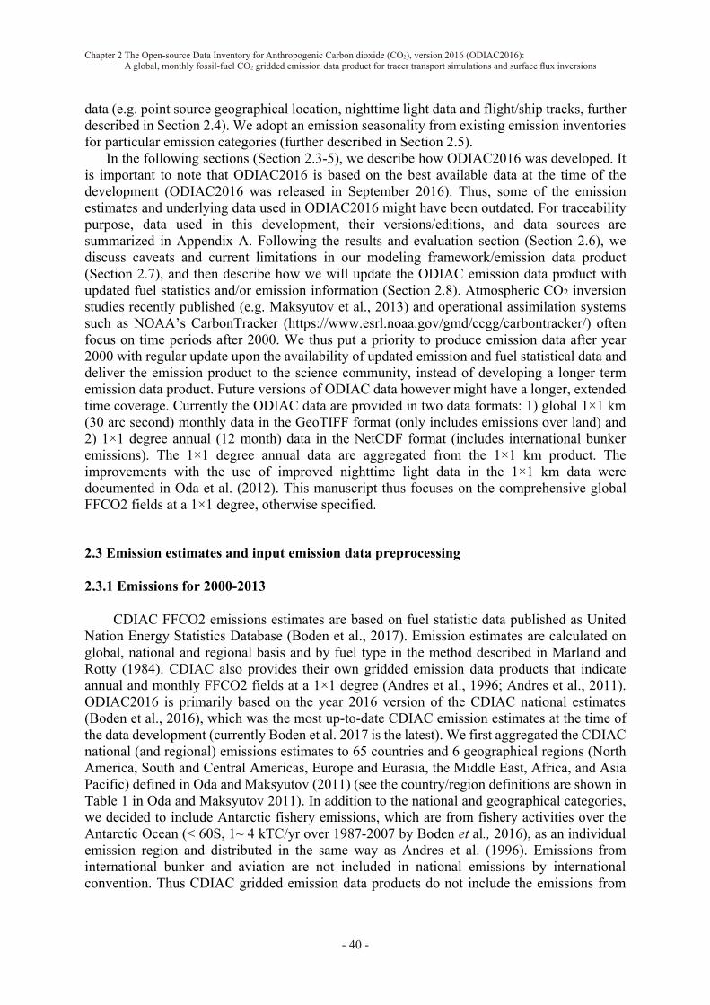
Chapter 2 The Open-source Data Inventory for Anthropogenic Carbon dioxide (CO2), version 2016
- 40 -
data (e.g. point source geographical location, nighttime light data and flight/ship tracks, further described in Section 2.4). We adopt an emission seasonality from existing emission inventories for particular emission categories (further described in Section 2.5). In the following sections (Section 2.3-5), we describe how ODIAC2016 was developed. It is important to note that ODIAC2016 is based on the best available data at the time of the development (ODIAC2016 was released in September 2016). Thus, some of the emission estimates and underlying data used in ODIAC2016 might have been outdated. For traceability purpose, data used in this development, their versions/editions, and data sources are summarized in Appendix A. Following the results and evaluation section (Section 2.6), we discuss caveats and current limitations in our modeling framework/emission data product (Section 2.7), and then describe how we will update the ODIAC emission data product with updated fuel statistics and/or emission information (Section 2.8). Atmospheric CO2 inversion studies recently published (e.g. Maksyutov et al., 2013) and operational assimilation systems such as NOAA’s CarbonTracker (https://www.esrl.noaa.gov/gmd/ccgg/carbontracker/) often focus on time periods after 2000. We thus put a priority to produce emission data after year 2000 with regular update upon the availability of updated emission and fuel statistical data and deliver the emission product to the science community, instead of developing a longer term emission data product. Future versions of ODIAC data however might have a longer, extended time coverage. Currently the ODIAC data are provided in two data formats: 1) global 1×1 km (30 arc second) monthly data in the GeoTIFF format (only includes emissions over land) and 2) 1×1 degree annual (12 month) data in the NetCDF format (includes international bunker emissions). The 1×1 degree annual data are aggregated from the 1×1 km product. The improvements with the use of improved nighttime light data in the 1×1 km data were documented in Oda et al. (2012). This manuscript thus focuses on the comprehensive global FFCO2 fields at a 1×1 degree, otherwise specified.
2.3 Emission estimates and input emission data preprocessing 2.3.1 Emissions for 2000-2013 CDIAC FFCO2 emissions estimates are based on fuel statistic data published as United Nation Energy Statistics Database (Boden et al., 2017). Emission estimates are calculated on global, national and regional basis and by fuel type in the method described in Marland and Rotty (1984). CDIAC also provides their own gridded emission data products that indicate annual and monthly FFCO2 fields at a 1×1 degree (Andres et al., 1996; Andres et al., 2011). ODIAC2016 is primarily based on the year 2016 version of the CDIAC national estimates (Boden et al., 2016), which was the most up-to-date CDIAC emission estimates at the time of the data development (currently Boden et al. 2017 is the latest). We first aggregated the CDIAC national (and regional) emissions estimates to 65 countries and 6 geographical regions (North America, South and Central Americas, Europe and Eurasia, the Middle East, Africa, and Asia Pacific) defined in Oda and Maksyutov (2011) (see the country/region definitions are shown in Table 1 in Oda and Maksyutov 2011). In addition to the national and geographical categories, we decided to include Antarctic fishery emissions, which are from fishery activities over the Antarctic Ocean (< 60S, 1~ 4 kTC/yr over 1987-2007 by Boden et al., 2016), as an individual emission region and distributed in the same way as Andres et al. (1996). Emissions from international bunker and aviation are not included in national emissions by international convention. Thus CDIAC gridded emission data products do not include the emissions from
Chapter 2 The Open-source Data Inventory for Anthropogenic Carbon dioxide (CO2), version 2016 (ODIAC2016): A global, monthly fossil-fuel CO2 gridded emission data product for tracer transport simulations and surface flux inversions
- 40 -

CGER-I143-2019, CGER/NIES
- 41 -
international bunker and aviation although the CDIAC/ORNL does have records of those emissions on national/regional basis. ODIAC2016 includes those emissions to achieve comprehensive global FFCO2 gridded emission fields. In CDIAC emission estimates, the global total emission and national total emissions are obtained by different calculation methods (global fuel production vs. apparent national fuel consumption, see Andres et al., 2012) and the CDIAC national totals do not sum to the CDIAC global total due to the difference in calculation method and inconsistencies in the underlying statistical data (e.g. import/export totals) (e.g. Andres et al., 2012). We thus calculate the difference between the global total and the sum of national totals and scaled up national totals to account for the difference. Andres et al. (2014) reported global total emission estimates calculated with production data (as opposed to apparent consumption data) have the smallest uncertainty (approximately 8% (2 sigma). It is thus used as the reference for global carbon budget analyses (e.g. Le Quéré et al., 2016). Inversion analysis is an extended version of the global carbon budget analysis using atmospheric models. We thus believe that imposing transport models and/or inversion models in a consistent way with the global carbon budget analysis such as Le Quéré et al. (2016) has significance, although we sacrifice the accuracy of the national/regional emission estimates. Due to the global scaling, national totals in ODIAC2016 differ from the estimates originally reported by the CDIAC/ORNL. The differences between the CDIAC global total and the sum of national emissions are often few percent and thus the magnitude of the scaling is often within the uncertainty range of national emissions (e.g. 4.0 to 20.2%, Andres et al., 2014). The global scaling factor derived and used in this study are presented in Appendix A2. 2.3.2 Emissions for 2014-2015 The year 2016 version of the CDIAC emission estimates only covers years to 2013 (Boden et al., 2016). We thus extrapolated the year 2013 CDIAC emissions to years 2014 and 2015 using the year 2016 version of the BP global fuel statistical data (BP, 2017). Our emission extrapolation approach is the same as Myhre et al. (2009) and Le Quéré et al. (2016). Emissions from cement production and gas flaring (approximately 5.7% and 0.6% of the 2013 global total, Boden et al., 2016) were assumed to be as the same as year 2013. International bunker emissions were scaled using changes in national total emissions. 2.3.3 CDIAC emission sector to ODIAC emission categories CDIAC national emission estimates (prepared by fuel type) were re-categorized to our own ODIAC emission categories (point source, nonpoint source, cement production, gas flare and international aviation and international marine bunker). Following Oda and Maksyutov (2011), the sum of emissions from liquid, gas and solid fuels was further divided into point source emissions and non-point source emissions. The total emissions from point sources were estimated using national total power plant emissions calculated using CARMA (Oda and Maksyutov, 2011). As mentioned earlier, CDIAC gridded emission data products only indicate national emissions and do not include international bunker emissions (Andres et al., 1996, Andres et al., 2011). In contrast, EDGAR provides bunker emissions in their gridded data product (JRC, 2017). Peylin et al. (2013) show some models include international bunker emissions and some do not, although the difference due to the inclusion/exclusion of the international bunker emissions in the prescribed emissions could be corrected afterwards (Peylin et al., 2013). In ODIAC2016, we carry CDIAC international bunker emissions reported
- 41 -

Chapter 2 The Open-source Data Inventory for Anthropogenic Carbon dioxide (CO2), version 2016
- 42 -
on country basis to achieve the complete picture of the global fossil fuel emissions. Country total bunker emissions (aviation plus marine bunker) were distributed using spatial proxy data adopted from other emission inventories described later (see Section 2.4.3). Although the CDIAC/ORNL does not report emissions from international aviation and marine bunker separately, we loosely estimated those two emissions using U.N. statistics. We estimated the fraction of aircraft emissions using jet fuel and aviation gasoline consumption and then the international bunker emissions were divided into aircraft and marine bunker emissions. 2.4 Spatial emission disaggregation 2.4.1 Emissions from point sources, non-point sources and cement production We define the sum of the emissions from solid, liquid and gas fuels as land emission (see Fig. 2. 1). Land emissions are further divided into two emission categories (point source emissions and non-point source emissions) and then distributed at a 1×1 km resolution in the ways described in Oda and Maksyutov (2011): Point source emissions are mapped using power plant profiles (emission intensity and geographical location) taken from the CARbon Monitoring and Action (CARMA) database (Wheeler and Ummel, 2008) and non-point source emissions are distributed using nighttime light data collected by the Defense Meteorological Satellite Program (DMSP) satellites (e.g. Elvidge et al., 1999). To avoid a difficulty in emission disaggregation especially over bright regions in nighttime light data (e.g. cities), Oda and Maksyutov (2011) employed a product that does not have an instrument saturation issue, rather than regular nightlight product. ODIAC2016 employs the latest version of the special nighttime light product (Ziskin et al., 2010). The improved nighttime light data has mitigated the underestimation of emissions over dimmer areas seen in ODIAC v1.7 (Oda et al., 2010). Nighttime light data are currently available for multiple years (1996-97, 1999, 2000, 2002-03, 2004, 2005-06 and 2010). In ODIAC2016, due to the lack of information, the emissions from cement production were spatially distributed as a part of non-point source emissions, although those emissions should have been distributed as point sources. This needs to be fixed in future versions of ODIAC emission data. 2.4.2 Emissions from gas flaring In the ODIAC v1.7, emissions from gas flaring were not considered (Oda and Maksyutov 2011). Nighttime light pixels corresponding to gas flares often appear very bright and would result in creating strong point sources in emission data (Oda and Maksyutov, 2011). We thus identified and excluded those bright gas flare pixels before distributing land emissions, using another global nighttime light data product that was specifically developed for gas flares by National Oceanic and Atmosphere Administration (NOAA), National Centers for Environmental Information (NCEI, former National Geophysical Data Center (NGDC)) (Oda and Maksyutov, 2011). In ODIAC2016 we separately distributed CDIAC gas flare emissions using the 1×1 km nightlight-based gas flare maps developed for 65 individual countries (Elvidge et al., 2009). Other than the 65 countries, the gas flare emissions were distributed as a part of land emissions.
Chapter 2 The Open-source Data Inventory for Anthropogenic Carbon dioxide (CO2), version 2016 (ODIAC2016): A global, monthly fossil-fuel CO2 gridded emission data product for tracer transport simulations and surface flux inversions
- 42 -
CGER-I143-2019, CGER/NIES
- 43 -
2.4.3 Emissions from international aviation and marine bunker Emissions from international aviation and marine bunker were distributed using aircraft and ship fleet tracks. International aviation emissions were distributed using the AERO2k inventory (Eyers et al., 2005). The AERO2k inventory was developed by a team at the Manchester Metropolitan University (MMU) and indicates the fuel use and NOx, CO2, CO, hydrocarbon and particulate emissions for 2002 and 2025 (projected) with injection height at a 1×1 degree spatial resolution on monthly basis. We used their column total CO2 emissions to distribute emissions to a single layer. International marine bunker emissions were distributed at a 0.1×0.1 degree using an international marine bunker emission map from the EDGAR v4.1(JRC, 2017). We decided not to adopt an international and domestic shipping (1A3d) map from EDGAR v4.2 as it includes domestic shipping emissions that we do not distinguish. 2.5. Temporal emission disaggregation The inclusion of the temporal variations is often a key in transport model simulation. For CO2 flux inversion, the potential biases in flux inverse emission estimates due to the lack of temporal profiles was suggested by Gurney et al. (2005). In ODIAC2016, we adopt the seasonal emission changes developed by Andres et al. (2011). The CDIAC monthly gridded data include monthly national emissions gridded at a 1×1 degree resolution (Andres et al. 2011). We normalized the monthly emission fields by the annual total and the applied to our annual emissions over land. The seasonality in ODIAC2016 is based on the year 2013 version of the CDIAC monthly gridded emission. The CDIAC monthly emission data do not cover the recent years. For recent years, we created a climatological seasonality using monthly CDIAC data from 2000-2010 (excepting 2009 where economic recession happened). Due to the limited availability of monthly fuel statistical data, Andres et al. (2011) used proxy country and also seasonality allocated by Monte Carlo simulations. The years between 2000-2010 were most data rich period and mostly explained by data (see Fig. 1 in Andres et al., 2011). Although ODIAC2016 only provides monthly emission fields, users can derive hourly emissions by applying scaling factors developed by Nassar et al. (2013). The Temporal Improvements for Modeling Emissions by Scaling (TIMES) is a set of scaling factors which one can derive weekly emissions and diurnal emissions from any monthly emission data that you use. Temporal profiles are collected from Vulcan, EDGAR and best available information and gridded on a 0.25×0.25 degree (Nassar et al., 2013). TIMES also includes per capita emissions corrections for Canada (Nassar et al., 2013). 2.6 Results and discussions 2.6.1 Annual global emissions In Fig. 2.2, global emission time series from different emission data were compared to give an idea of agreement among them. We calculated the global total for each year from four gridded emission data for the period of 2000-2016: CDIAC global total + projection (taken from ODIAC2016), CDIAC gridded data (hence, no international bunker emissions), two versions of EDGAR gridded data (v4.2 and FastTrack). The uncertainty range (shaded in tan) is 8% (2 sigma) estimated for CDIAC global by Andres et al. (2014). Those gridded emission
- 43 -

Chapter 2 The Open-source Data Inventory for Anthropogenic Carbon dioxide (CO2), version 2016
- 44 -
data are often used in global atmospheric CO2 inversion analysis (e.g. Peylin et al., 2013). To account for the difference in emission reporting categories (e.g. fuel basis in CDIAC vs. emission sector basis in EDGAR), the EDGAR totals were calculated as the “total short cycle C” emissions minus the sum of emissions from agriculture (IPCC code: 4C and 4D), land use change and forestry (5A, C, D, F and 4E) and waste (6C) (see more details on emission sectors documented in JRC (2017)). International aviation (1A3a) and navigation (1A3b) were thus included in values for EDGAR time series. The authors acknowledge the JRC has updated EDGAR emission time series for 1970-2012 in November 2014 (JRC, 2017). This study however uses gridded emission data, which are not fully based on the updated emission estimates, in order to characterize differences from gridded emission data, especially for potential data users in the modeling community. All four global total values obtained from four gridded emission data agree well within 8% uncertainty. The difference between ODIAC and CDIAC gridded data (3.3%-5.7%) were largely attributable to the international bunker emissions and global correction. ODIAC (where the total was scaled by CDIAC global total) and two versions EDGAR showed minor differences in magnitude (0.3%-2.7%) and trend, which are largely attributable to the differences in the underlying statistical data (e.g. U.N. Stat vs. EIA from different inventory years) and the emission calculation method (fuel basis vs. sector basis). Global total estimates at 5-year increments are shown in Table 2.1. For the year 2014 and 2015, we estimated the global total emissions 9.836 and 9.844 PgC. Boden et al. (2017) reported the latest estimate for year 2014 global total emission as 9.855 PgC. Our projected 2014 emission estimate was lower than the latest estimate by approximately 0.02 PgC (0.2%).
Figure 2.2 Global emission time series from four gridded emission data: CDIAC (red, 2000-2013) plus projected emissions (dashed maroon, 2014-2015) (values taken from ODIAC2016), CDIAC 1×1 degree (black, 2000-2013), EDGAR v4.2 (green, 2000-2008) and EDGAR v4.2 Fast Track (blue, 2000-2010). The values here are given in the unit of peta gram (= giga tonnes) carbon per year. The shaded area indicated in tan is a two-sigma uncertainty range (8%) estimated for CDIAC global total emission estimates by Andres et al. (2014).
Figure 2.2 Global emission time series from four gridded emission data: CDIAC (red, 2000-2013) plus projected emissions (dashed maroon, 2014-2015) (values taken from ODIAC2016), CDIAC 1×1 degree (black, 2000-2013), EDGAR v4.2 (green, 2000-2008) and EDGAR v4.2 Fast Track (blue, 2000-2010). The values here are given in the unit of peta gram (= giga tonnes) carbon per year. The shaded area indicated in tan is a two-sigma uncertainty range (8%) estimated for CDIAC global total emission estimates by Andres et al. (2014).
Chapter 2 The Open-source Data Inventory for Anthropogenic Carbon dioxide (CO2), version 2016 (ODIAC2016): A global, monthly fossil-fuel CO2 gridded emission data product for tracer transport simulations and surface flux inversions
- 44 -

CGER-I143-2019, CGER/NIES
- 45 -
Table 2.1 Global total emission estimates for year 2000, 2005 and 2010 from four gridded emission data (ODIAC2016, CDIAC, EDGAR v4.2 and EDGAR FastTrack). Values for two versions of EDGAR emission data were calculated by subtracting emissions from agriculture (IPCC code: 4C and 4D), land use change and forestry (5A, C, D, F and 4E) and waste (6C) from the total EDGAR CO2 emissions (total short cycle C).
Year ODIAC2016 CDIAC
national EDGAR v4.2 EDGAR FT
2000 6727 6506 (-3.3%) 6907 (+2.7%) N/A 2005 8025 7592 (-5.4%) 8005 (-0.2%) 7959 (-0.8%) 2010 9137 8694 (-4.8%) N/A 8950 (-2.0%)
Fig. 2.3 shows the same type of comparison as Fig. 2.2., but for the top 10 emitting countries (China, US, India, Russian Federation, Japan, Germany, Islamic Republic of Iran, Republic of Korea (South Korea), Saudi Arabia and Brazil, according to the year 2013 ranking reported by CDIAC). We aggregated all the four gridded emission fields to a common 1×1 degree field and sampled using the 1×1 degree country mask used in CDIAC emission data development. The annual uncertainty estimates for national total emissions (2 sigma) are made following the method described by Andres et al., (2014) and values are shown in Table 2.2. In the analysis presented in Fig. 2.3, emissions from international aviation (1A3a) and navigation (1A3b) are excluded. All four national total values sampled from four gridded emission data at a 1×1 degree often agree within the uncertainty estimated by Andres et al. (2014). Systematic differences of ODIAC from CDIAC gridded data can be largely explained by 1) global correction (the total was scaled using CDIAC global total) and 2) the differences in emissions disaggregation methods. Although ODIAC is expected to indicate slightly higher values than CDIAC gridded data (often a few percent) because of the global correction (note global correction can be negative, despite of the depiction in Fig. 2.1), ODIAC sometimes indicates values lower that CDIAC gridded data more than few percent (see Japan in Fig. 2.3 as an example). This is due to a sampling error using the 1×1 degree country map in the analysis. The aggregated 1×1 degree ODIAC field is slightly larger than that of CDIAC especially because of the coastal areas depicted a high-resolution in the original 1×1 km emission field. This type of sampling error was discussed in Zhang et al. (2014). ODIAC employs a 1×1 km coastline and a 5×5 km country mask as described in Oda and Maksyutov (2011). Thus, the use of 1×1 degree CDIAC country map results in missing some land mass (hence, CO2 emissions). Similar sampling errors can happen for countries that are physical small and island countries, depending on the resolution of analysis. Despite of the sampling errors, the authors used the CDIAC 1×1 degree country map to do this comparison analysis with having CDIAC gridded data as a reference. The lower emission indicated by ODIAC or EDGAR in this analysis does not always mean the national total emissions are lower. The emission estimates at national level often agree well even among different emission inventories (e.g. Andres et al., 2012).
Table 2.1 Global total emission estimates for year 2000, 2005 and 2010 from four gridded emission data (ODIAC2016, CDIAC, EDGAR v4.2 and EDGAR FastTrack). Values for two versions of EDGAR emission data were calculated by subtracting emissions from agriculture (IPCC code: 4C and 4D), land use change and forestry (5A, C, D, F and 4E) and waste (6C) from the total EDGAR CO2 emissions (total short cycle C).
- 45 -

Chapter 2 The Open-source Data Inventory for Anthropogenic Carbon dioxide (CO2), version 2016
- 46 -
Figure 2.3 National emission time series for top 10 emitting countries (China, U.S., India, Russian Federation, Japan, Germany, Islamic Republic of Iran, Republic of Korea (South Korea), Saudi Arabia and Brazil). The values are given in the unit of peta gram (=giga tonnes) carbon per year. The values are calculated using gridded emission data, not tabular emission data. The national total values in the plots might be thus different from values indicated in the tabular form due to the emission disaggregation. The shaded area in grey indicates a two-sigma uncertainty range estimated by Andres et al. (2014) (see Table 2.2).
Chapter 2 The Open-source Data Inventory for Anthropogenic Carbon dioxide (CO2), version 2016 (ODIAC2016): A global, monthly fossil-fuel CO2 gridded emission data product for tracer transport simulations and surface flux inversions
- 46 -

CGER-I143-2019, CGER/NIES
- 47 -
Table 2.2 Annual uncertainty estimates associated with CDIAC national emission estimates. The uncertainty estimates were made following the method described by Andres et al. (2014). The national total emissions for the year 2013 were taken from Boden et al. (2016).
Ranking #
Country 2013 emissions in kTC (% of the global total)
Uncertainty (%)
1 China 2,795,054 (28.6%) 17.5 2 U.S. 1,414,281 (14.5%) 4.0 3 India 554,882 (5.7%) 12.1 4 Russia Federation 487,885 (5.0%) 14.8 5 Japan 339,074 (3.5%) 4.0 6 Germany 206,521 (2.1%) 4.0 7 Islamic Republic of
Iran 168,251 (1.7%) 9.4
8 Republic of Korea 161,576 (1.7%) 12.1 9 Saudi Arabia 147,649 (1.5%) 9.4 10 Brazil 137,354 (1.4%) 12.1
2.6.2 Global emission spatial distributions The global total emission fields of CDIAC gridded emission data and ODIAC2016 for the year 2013 (the most recent year CDIAC indicates) are shown in Fig. 2.4. Emission fields are shown at a common 1×1 degree. The major difference seen between two fields is primarily due to inclusion/exclusion of emissions from international bunker emissions that largely account for the differences indicated in Table 2.1. A breakdown of ODIAC year 2013 emission field are presented by emission category in Fig. 2.5. The emission fields for point sources, non-point sources, cement production and gas flaring were produced at a 1×1 km resolution in ODIAC 3.0 model, but as mentioned earlier, we focus on the 1×1 degree version of ODIAC2016 in this manuscript. In CDIAC gridded emission data, the emissions over land are distributed by population data without fuel type distinction. In ODIAC 3.0 model, we have added additional layers of consideration in the emission modeling from the conventional CDIAC model and add the possibility of future improvement with improved emission proxy data.
Table 2.2 Annual uncertainty estimates associated with CDIAC national emission estimates. The uncertainty estimates were made following the method described by Andres et al. (2014). The national total emissions for the year 2013 were taken from Boden et al. (2016).
- 47 -

Chapter 2 The Open-source Data Inventory for Anthropogenic Carbon dioxide (CO2), version 2016
- 48 -
Figure 2.4 Year 2013 global fossil fuel CO2 emissions distributions from CDIAC (left, 9.23 PgC) and ODIAC (right, 9.78 PgC). The ODIAC emission field was aggregated to a common 1 × 1 degree resolution. The value is given in the unit of log of thousand tonnes C/cell.
Figure 2.5 Year 2013 global distributions of ODIAC fossil fuel emissions by emission type. The panels show emissions from (from top to the right, then down) point source, non-point source, cement production, gas flaring, international aviation and international shipping. The values in the figures are given in the unit of log of thousand tonnes carbon/year/cell (1×1 degree). The numbers in the brackets are the total for the category emissions in the unit of PgC (total year 2013 emission in ODIAC2016 was 9.78 PgC).
Chapter 2 The Open-source Data Inventory for Anthropogenic Carbon dioxide (CO2), version 2016 (ODIAC2016): A global, monthly fossil-fuel CO2 gridded emission data product for tracer transport simulations and surface flux inversions
- 48 -
CGER-I143-2019, CGER/NIES
- 49 -
In Fig. 2.6., we compared the four global gridded products over land and also calculated differences from ODIAC2016 (shown in Fig. 2.7. Histograms are presented in Appendix A3). It is often very challenging to evaluate the accuracy and uncertainty of gridded emission data, because of the lack of direct physical measurements at grid scales (Andres et al., 2016). Recent studies have attempted to evaluate the uncertainty of gridded emission data by comparing emission data each other (e.g. Oda et al., 2015; Hutchins et al., 2016). The differences among emission were used as a proxy for uncertainty. However, it is important note that such evaluation does not give us an objective measure of which one is closer to truth, beyond characterizing the differences in emission spatial patterns and magnitudes from methodological viewpoints (e.g. emission estimation and disaggregation). Some of the gridded emission data are partially disaggregated using commercial information, which users are often not authorized to fully disclose the information used and thus makes the comparison even less meaningful and/or significant. Oda et al. (2015) also discussed that emission inter-comparison approaches often do not allow us to evaluate two distinct uncertainty sources (emissions and disaggregation) separately. In addition, because of the use of emission proxy for emission disaggregation (rather than mechanistic modeling), such comparison can be only implemented at an aggregated, coarse spatial resolution. These issues will be further discussed in the Section 2.7. Because of the limitation mentioned above, we here compared emission data only to characterize the differences that can be explained by the differences in emission disaggregation methods. We implemented this comparison exercise using 2008 emission field aggregated at a 1×1 degree resolution. Year 2008 is the most recent year where all the four emission fields are available. The major emission spatial patterns (e.g. emitting regions such as North America, Europe and East Asia) are overall very similar as the correlations were driven by national emission estimates (which we already saw good agreement earlier), but we do see differences due to emission disaggregation at the subnational level. Because of the use of nightlight, ODIAC did not indicate emissions over some of the areas (e.g. Africa and Eurasia) while others do. Especially, EDGAR has emissions over those areas that are largely explained by line source emissions such as transportation. Overall, ODIAC tends to put more emissions towards populated areas than suburbs. This is also explained by the lack of line sources. In EDGAR v4.2, domestic fishery emissions can be seen, but not in EDGAR FT. Even in these two EDGAR versions, we can confirm the subnational differences at United States, Europe and China.
- 49 -

Chapter 2 The Open-source Data Inventory for Anthropogenic Carbon dioxide (CO2), version 2016
- 50 -
Figure 2.6 Land emissions from ODIAC (upper left), CDIAC (upper right), two versions of EDGAR emission data (v4.2 lower left and v4.2 Fast Track lower right). The units are million tonnes carbon/year/cell (1×1 degree). In addition to excluding emissions from international aviation and marine bunker, some of the sector emissions were subtracted from EDGAR short cycle total emissions to account for the differences in emission calculation methods between CDIAC and EDGAR, as also done earlier. The emission fields for the year 2008 were used.
Figure 2.6 Land emissions from ODIAC (upper left), CDIAC (upper right), two versions of EDGAR emission data (v4.2 lower left and v4.2 Fast Track lower right). The units are million tonnes carbon/year/cell (1×1 degree). In addition to excluding emissions from international aviation and marine bunker, some of the sector emissions were subtracted from EDGAR short cycle total emissions to account for the differences in emission calculation methods between CDIAC and EDGAR, as also done earlier. The emission fields for the year 2008 were used.
Chapter 2 The Open-source Data Inventory for Anthropogenic Carbon dioxide (CO2), version 2016 (ODIAC2016): A global, monthly fossil-fuel CO2 gridded emission data product for tracer transport simulations and surface flux inversions
- 50 -

CGER-I143-2019, CGER/NIES
- 51 -
Figure 2.7 ODIAC-other emission data differences. CDIAC (upper right), two versions of EDGAR (v4.2 lower left and v4.2 Fast Track lower right). The units are million tonnes carbon/year/cell (1×1 degree). Note that the differences are defined as ODIAC (this study) minus others. The histograms of the differences are also presented in Appendix A3.
- 51 -

Chapter 2 The Open-source Data Inventory for Anthropogenic Carbon dioxide (CO2), version 2016
- 52 -
2.6.3 Regional emission time series. Fig. 2.8 shows time series of regional fossil fuel emissions aggregated over 11 land regions defined in the TransCom transport model intercomparison experiment (e.g. Gurney et al., 2002). The global seasonal variation and the associated uncertainty have been presented and discussed in Andres et al. (2011). Here monthly total emission values were calculated for eleven TransCom land regions and presented with the associated uncertainty values (see Table 2.3.). The monthly total values were calculated in both excluding international bunker emissions (hence, land emissions only) and including the emissions. The uncertainty range was calculated by mass weighted uncertainty estimates of countries that fall into the TransCom regions. The uncertainty ranges shown in Fig. 2.8. are annual uncertainty plus the monthly profile uncertainty (12.8%, reported by Andres et al., 2011). Monthly time series are presented for land only emissions and land and international bunker emission (here, largely aviation emissions). As described earlier, the emission seasonality was adopted from Andres et al. (2011). The patterns in the emission seasonality are often largely characterized by the large emitting countries within the regions (e.g. U.S. for region 2; China for region 8). Since Andres et al. (2011) used geographical closeness (also, type of economic systems) to define proxy countries, the countries in the same TransCom regions can have similar or the same seasonal patterns in their emissions. As we can see in Fig. 2.4. (panel plot for aviation emissions), aviation emissions are intense over North America, Europe and Asia. Global total aviation emission was approximately 0.12 PgC/yr in 2013 and it often does not account for a large portion of the global total (1.2% of the global total in 2013). However, considering the fact that those emissions are concentrated in particular areas such as North America, Europe and East Asia, rather than evenly distributed in space, and often imposed at the surface layer in transport model simulation, care must be taken to achieve an accurate atmospheric CO2 transport model simulation (Nassar et al., 2010). Aviation emissions were often around 0.5-5.1% of the land total emissions over the most regions, but as large as 12.7% (North American Boreal).
Chapter 2 The Open-source Data Inventory for Anthropogenic Carbon dioxide (CO2), version 2016 (ODIAC2016): A global, monthly fossil-fuel CO2 gridded emission data product for tracer transport simulations and surface flux inversions
- 52 -

CGER-I143-2019, CGER/NIES
- 53 -
Figure 2.8 Emission time series over inversion analysis land regions defined by the Transport
model intercomparison (TransCom) project (Gurney et al., 2002). The TransCom region map (bottom right) is available from http://transcom.project.asu.edu/transcom03_protocol_basisMap.php (last access: 8 November, 2016). Black lines indicate the ODIAC 1×1 degree monthly emissions. The monthly emissions are calculated using the 1×1 degree ODIAC emission data. The uncertainty range was calculated by mass weighted uncertainty estimates of countries that fall into the regions (see Table 2.3). The uncertainty ranges shown in Fig. 2.8 are annual uncertainty plus the monthly profile uncertainty (12.8%, reported by Andres et al., 2011). Note scales in the vertical axis are different.
- 53 -

Chapter 2 The Open-source Data Inventory for Anthropogenic Carbon dioxide (CO2), version 2016
- 54 -
Table 2.3 Annual total emission over the TransCom land regions and the associated uncertainty estimates. The total emissions were calculated using the ODIAC2016 gridded emission data. The numbers in the bracket are values including international bunker emissions. The uncertainty estimates were mass weighted values of uncertainty estimates of countries that fall in the regions. Country uncertainty estimates were estimated using the method described Andres et al. (2014). The values were reported as the 2-sigma uncertainty.
Region # Region name Uncertainty
(%)
1 North American Boreal 3.7
2 North American Temperate
3.7
3 South American Tropical 9.6
4 South American Temperate
12.8
5 Northern Africa 5.1
6 Southern Africa 10.6
7 Eurasian Boreal 12.4
8 Eurasian Temperate 7.8
9 Tropical Asia 11.8
10 Australia 4.0
11 Europe 3.8 2.7 Current limitations, caveats and future prospects As ODIAC emission data product is now used for a wide variety of the carbon cycle research (e.g. global, regional inversions, urban emission studies), it would be useful for the users of the ODIAC emission data product to note and discuss issues, limitations and caveats in our emission data that the authors are aware. Some of the issues and limitations are specific to our study, however the majority of them are often shared by other existing gridded emission data and or emission models. 2.7.1 Emission estimates In the production of ODIAC2016, we used several versions/editions of CDIAC estimates (e.g. global estimates, national estimates and monthly gridded data). This could often happen in emission data production, as some of the underlying data are not updated/upgraded at the time of emission data production (we often start updating emission data after new fuel statistical data are released). We sometimes accept the inconsistency and try to use the most up-to-date information available. For example, we could use GCP’s emission estimates (e.g. Le Quéré et
Table 2.3 Annual total emission over the TransCom land regions and the associated uncertainty estimates. The total emissions were calculated using the ODIAC2016 gridded emission data. The numbers in the bracket are values including international bunker emissions. The uncertainty estimates were mass weighted values of uncertainty estimates of countries that fall in the regions. Country uncertainty estimates were estimated using the method described Andres et al. (2014). The values were reported as the 2-sigma uncertainty.
Chapter 2 The Open-source Data Inventory for Anthropogenic Carbon dioxide (CO2), version 2016 (ODIAC2016): A global, monthly fossil-fuel CO2 gridded emission data product for tracer transport simulations and surface flux inversions
- 54 -

CGER-I143-2019, CGER/NIES
- 55 -
al., 2016) to constrain the global totals, if CDIAC global total emission estimates are not available. The way we obtained emission estimates for each version is often described in the NetCDF header information of the emission data product. The use of the CARMA power plant estimates for estimating magnitude of point source portion of emissions is hard to eliminate, although ideally this is done using emission estimates that are fully compatible to CDIAC estimates. We are currently examining U.N. statistical data (which CDIAC emission estimates are based on) to assess the ability of explaining power plant emissions. 2.7.2 Emission spatial distributions 2.7.2.1 Point source emissions Although the use of the power plant geolocation allowed us to achieve improved high-resolution emission spatial distributions over land (Oda and Maksyutov, 2011), the availability of power plant data is often very limited. For example, CARMA does not provide power plant emissions and its status (e.g. commission/decommission) every year and furthermore update/upgrade after their version 3.0 database (which dated 2012). The error in their power plant geolocation is another issue that has been identified (e.g. Oda and Maksytuov, 2011; Woodard et al., 2015). In ODIAC, the base year emissions (2007) were projected and all the power plants were assumed to be active over the period (Oda and Maksyutov, 2011). There are only few global projects that are collecting power plant information such as the Global Energy Observatory (GEO, http://globalenergyobservatory.org/) and those can be a useful source of data to improve and supplement CARMA database. Regionally, CARMA can be evaluated using an inventory such as the U.S. Emissions and Generation Resource Integrated Database (eGRID) (EPA, 2017). However, it is often difficult to find such a well-constructed and documented inventory for countries that are actually driving the uncertainty in global emissions (e.g. China and India). Emissions from cement production (which are currently distributed using nightlight by Ziskin et al., 2010) and gas flare (which is distributed using gas flare nightlight data by Elvidge et al., 2009) should be distributed as point sources. For gas flare emissions, we are examining the use of Nightfire (Elvidge at al., 2013a) to pinpoint active gas flares in timely manner and improve their emissions spatial disaggregation over the recent years. Currently, the point source emissions in ODIAC do not have an injection height due to the lack of global information. This limitation is shared with other existing global emission data products. 2.7.2.2 Non-point source emissions Nighttime light data has been an excellent proxy for human settlements (hence, CO2 emissions) even at a high spatial resolution, however there are some issues to be discussed. As mentioned earlier, we used an improved version of calibrated radiance data developed by Ziskin et al. (2010), but those data are only available to seven data periods over the course of DMSP years (1992-2013). As we do not believe linearly interpolating the existing nightlight data over the intervening years is necessarily the best way (as done in Asefi-Najafabady et al., 2014), the same nightlight data has been used for some periods and thus emission distributions remain unchanged. We are now examining the use of nightlight data collected from the Visible Infrared Imaging Radiometer Suite (VIIRS) on Suomi National Polar-orbiting Partnership satellite (e.g. Elvidge et al., 2013b; Román and Stokes, 2015). VIIRS instruments do not have several critical issues that the DMSP instrument had (e.g. spatial resolution, dynamic range, quantization and
- 55 -

Chapter 2 The Open-source Data Inventory for Anthropogenic Carbon dioxide (CO2), version 2016
- 56 -
calibration) (Elvidge et al., 2013b). The fully calibrated nightlight data can be used to map emission changes in space in timely and consistent manner. In ODIAC, the disaggregation of non-point emissions is solely done using nighttime light data for estimating subnational emission spatial distributions and no additional subnational emission constrain were applied. Rayner et al. (2010) proposed to better constrain subnational emission spatial distribution by combining population data, nighttime lights and GDP in their Fossil Fuel Data Assimilation System (FFDAS) framework. Asefi-Najafabady et al. (2014) further introduced the use of point source information in their disaggregation, the optimization in their current framework is however under-constrained by the lack of GDP information. Without having such optimization, the state level per capita emission estimates can provide subnational constraints. Nassar et al. (2013) evaluated the per capita emissions in CDIAC and ODIAC emission data over Canada using the national inventory and found that ODIAC outperformed. However, as the nightlight-population relationship might have a bias for developing and the least developed countries (Raupach et al., 2010), we would expect we see significant biases over those countries and the per capita estimates can provide a useful constraint. As seen in the comparison to other emission data, the major difference from EDGAR emission spatial distribution was due to the lack of line sources in ODIAC. We do not believe the result from the emission data comparison can falsify the emission distribution in ODIAC, as discussed earlier. However, we do expect an inclusion of the line sources would improve the spatial distributions and emission representations in both cities and rural areas. We are currently examining the inclusion of transportation network data (e.g. OpenStreetMap) as proxy for line source emissions to explore the better spatial emission aggregation method. Oda et al. (2017) recently implemented the idea of adding a spatial proxy for line sources and improved emission estimates for a U.S. city. 2.7.2.3 Aviation emissions We estimated emissions from international aviation from CDIAC using U.N. statistical data. The emissions are currently provided as a single layer emission field, although it is not appropriate given the nature of the aviation emissions. Nassar et al. (2010) discussed that the importance of the three dimensional (e.g. x,y,z) emissions for interpreting CO2 profile. In current modeling framework, although we maintain the aviation emission injection height from AERO2k (reduced to 1km interval), we distribute the emissions to a single layer. As pointed out by Olsen et al. (2013), AERO2k does not agree with other inventories in height distribution. With noting the caution, we will examine the use of height information from AERO2k and other data available to us and do sensitivity analysis using transport model simulations. 2.7.3 Emission temporal profiles. The emission seasonality in ODIAC2016 is based on Andres et al. (2011) and it can be further extended using the TIMES scaling parameter to hourly scale. We note that the emission seasonality was based on top 10 emitting countries’ fuel statistics and Monte Carlo simulation (Andres et al., 2011). The emission seasonality for countries other than the top 10 could be less robust. Also, because of the use of Monte Carlo, the seasonality is different over different editions of monthly emission data. It is also important to note that the repeated use of climatological (mean) seasonality for the recent years (described in Section 2.5) could be a source of uncertainty and biases. Andres et al. (2011) estimated the monthly uncertainty as
Chapter 2 The Open-source Data Inventory for Anthropogenic Carbon dioxide (CO2), version 2016 (ODIAC2016): A global, monthly fossil-fuel CO2 gridded emission data product for tracer transport simulations and surface flux inversions
- 56 -

CGER-I143-2019, CGER/NIES
- 57 -
12.8% (two sigma) in addition to the annual emission uncertainty. As we often impose fossil fuel emissions, a care must be taken when applied to inversions. Ultimately, as done by Vogel et al. (2013), we might be able to evaluate temporal profiles from statistical data and improve them (but only to limited small locations). 2.7.4 Uncertainties associated with gridded emission fields As mentioned earlier, the evaluation of gridded emission data is often very challenging and most of the emission data study share this difficulty. Although the emission estimates are made at global and national scales with small uncertainties (e.g. 8% for global by Andres et al., 2014), considerable errors seem to be introduced when the emissions are disaggregated (e.g. Hogue et al., 2016; Andres et al., 2016). Andres et al. (2016) for example estimated the uncertainty associated with CDIAC gridded emission data on a per grid cell basis with an average of 120% and a range of 4.0 to 190% (2 sigma). Hogue et al. (2016) closely looked at CDIAC gridded emission data over the U. S. domain and estimated the uncertainty associated with the 1×1 degree emission grids as ±150%. Those errors seem to be unique to the disaggregation method (Andres et al., 2016). Future funding may allow us to pursue a full uncertainty analysis of the ODIAC emission data/model, akin to the Andres et al. (2016) approach but accounting for the greater than one carbon distribution mechanisms utilized in the ODIAC emission modeling framework. All of the spatially distributed gridded emission data mentioned in this manuscript suffer from the same basic defect: they use proxies to spatially distribute emissions rather than actual measurements. In addition, evaluating emission distributions based on a nightlight proxy can be challenging as the connection between CO2 emissions and proxy is less direct compared to population (e.g. per capita emissions). A combined use of emission proxy and geolocation data (e.g. power plant location) would also add additional difficulties to give a comprehensive measure of the uncertainty because of different type of error/uncertainty sources (e.g. Woodard et al., 2015). As finer spatial scales are approached, the defect of the proxy approach becomes more apparent: proxies only estimate emission fields. The ODIAC data product has been used not only for global simulations at an aggregated spatial resolution, but also at very high spatial resolution (e.g. Ganshin et al. 2010; Oda et al. 2012; Lauvaux et al. 2016; Oda et al. 2017). Thus, an emission evaluation at a high resolution has become an important task. One approach we could take for evaluating high-resolution emission fields is comparing to a local fine-grained emission data product such as Gurney et al. (2012), acknowledging the limitations of the approach discussed earlier. Another approach would be evaluating emission data in concentration space, rather than emission space. As reported in Vogel et al. (2013) and Lauvaux et al. (2016), with radiocarbon measurements and/or good, spatially dense CO2 measurements, a high-resolution transport model simulation can provide an objective measure for emission data evaluations (e.g. model-observation mismatch and emission inverse estimate). While the quality (i.e. bias and uncertainty) of the gridded emission estimates remains unquantified for most of the emission data mentioned in this manuscript, the emission data are still used because sufficient measurements in space and time are not presently available to offer a better alternative. At very least, we presented the uncertainty estimates over the aggregated TransCom land regions. We believe that the regional uncertainty estimates are highly useful for atmospheric CO2 inversion modelers, more than uncertainty estimates at a grid level, which still do not seem to be ready for use. Inversion studies often aggregate flux estimates over the TransCom land regions to interpret regional carbon budgets, while flux estimations in their models are done at much higher spatial resolutions (e.g. Feng et al., 2009; Chevallier et al., 2010; Basu et al., 2013). Taking an advantage of being based on the CDIAC estimates, we
- 57 -
Chapter 2 The Open-source Data Inventory for Anthropogenic Carbon dioxide (CO2), version 2016
- 58 -
adopted the updated uncertainty estimates reported by Andres et al. (2016) and obtained the regional uncertainty estimates. Those estimates are new and readily usable to the inversion studies especially when interpreting the regional estimates. 2.8 Product distribution, data policy and future update The ODIAC2016 data product is available from a website hosted by the Center for Global Environmental Research (CGER), Japanese National Institute for Environmental Studies (NIES) (http://db.cger.nies.go.jp/dataset/ODIAC/, doi: 10.17595/20170411.001). The data product is distributed under Creative Commons Attribution 4.0 International (CC-BY 4.0, https://creativecommons.org/licenses/by/4.0/deed.en). The ODIAC2016 emission data are provided in two file formats: 1) global 1×1 km (30 arc second) monthly file in the GeoTIFF format (only includes emissions over land) and 2) 1×1 degree annual (12 month) file in the NetCDF format (includes international bunker emissions). A single, global 1×1 km monthly GeoTIFF file is about 3.7 GB (compressed to 120 MB). A 1×1 degree single NetCDF annual file is about 6MB. We update the emission data on annual basis, following a release of an updated global fuel statistical data. Future versions of the emissions data are in principle based on updated version/edition of the underlying statistical data with the same name convention (ODIACYYYY, YYYY= the release year, the end year is YYYY minus 1). In October 2017, we started distributing the updated, year 2017 version of ODIAC data (ODIAC2017, 2000-2016). We primarily focus on years after 2000. Future versions of ODIAC data however might have a longer, extended time coverage. 2.9 Summary This manuscript describes the year 2016 version of ODIAC emission data (ODIAC2016) and how the emission data product was developed within our upgraded emission modeling framework. Based on the CDIAC emission data, ODIAC2016 can be viewed as an extended version of the CDIAC gridded data with improved emission spatial distributions representations. Utilizing the best available data (emission estimates and proxy), we achieved a comprehensive, global fossil fuel CO2 gridded emission field that allows data users to impose their CO2 simulations in a consistent way with many of the global carbon budget analysis. With updated fuel statistics, we should be able to continue producing an updated, future versions of ODIAC emission data product within the same model framework. The capability we developed in this study has become more significance now, given the CDIAC/ORNL’s shutdown. Despise of expected difficulties (e.g. discontinued CDIAC estimates), the authors believe that ODIAC could play an important role in delivering emission data to the carbon cycle science community. Limitations and caveats discussed in this manuscript mirror and lead ODIAC’s future prospects. The ODIAC emission data product is distributed from http://db.cger.nies.go.jp/dataset/ODIAC/ with a DOI. Currently the 2017 version of ODIAC emission data (ODIAC2017, 2000-2016) is also available.
Chapter 2 The Open-source Data Inventory for Anthropogenic Carbon dioxide (CO2), version 2016 (ODIAC2016): A global, monthly fossil-fuel CO2 gridded emission data product for tracer transport simulations and surface flux inversions
- 58 -

CGER-I143-2019, CGER/NIES
- 59 -
Appendix 2.A
Table 2.A1 A list of components in ODIAC2016 and data used in the development.
Component
Data/product name
Description and data source Reference
Global FFCO2
CDIAC global fossil-fuel CO2 emissions
The year 2016 edition of the CDIAC global total estimates were used to constrain the ODIAC2016 totals. Data available at http://cdiac.ornl.gov/ftp/ndp030/global.1751_2013.ems.
Boden et al. (2016)
National FFCO2
CDIAC fossil-fuel CO2 emissions by Nation
The year 2016 editions of the CDIAC national emission estimates are used as a primary input data. Data available at http://cdiac.ornl.gov/ftp/ndp030/nation.1751_2013.ems.
Boden et al. (2016)
Global fuel statistics
BP Statistical review of world energy
The year 2016 edition of the BP statistical data were used to project CDIAC national emissions over the recent years (2014-2015). Data are available at http://www.bp.com/en/global/corporate/energy-economics/statistical-review-of-world-energy.html.
BP (2017)
Monthly temporal variation
CDIAC Gridded Monthly Estimate
The year 2013 version of the CDIAC monthly gridded data were used to the model seasonality in ODIAC2016. Data are available at http://cdiac.ornl.gov/ftp/fossil_fuel_CO2_emissions_gridded_monthly_v2013/
Andres et al. (2011)
Power plant data
CARMA The CARMA power plant database with geolocation correction described in Oda and Maksyutov (2011). Data available from http://carma.org/.
Wheeler and Ummel et al. (2008)
NTL (for non-point emissions)
Global Radiance Calibrated Nighttime Lights
Multiple year NTL data are used to distribute nonpoint emissions. Data are available at https://ngdc.noaa.gov/eog/dmsp/download_radcal.html.
Ziskin et al. (2010)
- 59 -

Chapter 2 The Open-source Data Inventory for Anthropogenic Carbon dioxide (CO2), version 2016
- 60 -
NTL (for gas flaring)
Global Gas Flaring Shapefiles
Global gas flaring NTL data are specifically used to distribute gas flaring emissions. Data are available at http://ngdc.noaa.gov/eog/interest/gas_flares_countries_shapefiles.html
Elvidge et al. (2009)
Int’l ship tracks
EDGAR v4.1
The international marine bunker emission field in EDGAR v4.1 was used. Data are available at http://edgar.jrc.ec.europa.eu/archived_datasets.php.
JRC (2017)
Int’l Aviation flight tracks
AERO2k Data were used to distributed aviation emissions. More details can be find at http://www.cate.mmu.ac.uk/projects/aero2k/.
Eyers et al. (2005)
Weekly and diurnal cycle
TIMES This was not a part of ODIAC2016, however it is useful to note that this scaling factors can be used to create weekly and diurnally varying emissions. Data are available at http://cdiac.ornl.gov/ftp/Nassar_Emissions_Scale_Factors/.
Nassar et al. (2013)
Appendix 2.A2
Table 2.A2 A table for the global scaling factor for 2000-2013.
Year Scaling factor2000 0.999 2001 1.016 2002 1.008 2003 1.014 2004 1.012 2005 1.022 2006 1.022 2007 1.016 2008 1.023 2009 1.024 2010 1.015 2011 1.017 2012 1.017 2013 1.025
Chapter 2 The Open-source Data Inventory for Anthropogenic Carbon dioxide (CO2), version 2016 (ODIAC2016): A global, monthly fossil-fuel CO2 gridded emission data product for tracer transport simulations and surface flux inversions
- 60 -

CGER-I143-2019, CGER/NIES
- 61 -
Appendix 2.A3
Fig. 2.A3 A histogram of the inter-emission data differences from ODIAC. Values are given in the
unit of million tonnes carbon per year (MTC/yr). Acknowledgments
TO is supported by NASA Carbon Cycle Science program (Grant # NNX14AM76G). RJA is now retired but this work was sponsored by U.S. Department of Energy, Office of Science, Biological and Environmental Research (BER) programs and performed at the Oak Ridge National Laboratory (ORNL) under U.S. Department of Energy contract DE-AC05-00OR22725. The authors would like to thank Chris Elvidge and Kim Baugh at NOAA/NGDC for providing the nightlight data. The authors also thank Yasuhiro Tsukada and Tomoko Shirai for hosting the ODIAC emission data on the data server at NIES.
References Andres, R. J., Marland, G., Fung, I., Matthews, E. (1996) A 1° × 1° distribution of carbon dioxide emissions from
fossil fuel consumption and cement manufacture, 1950–1990. Global Biogeochem. Cy., 10(3), 419–429, doi:10.1029/96GB01523.
Andres R. J., Gregg J. S., Losey, L., Marland, G., Boden, T.A. (2011) Monthly, global emissions of carbon dioxide from fossil fuel consumption. Tellus B, 63, 309-327, doi:10.1111/j.1600-0889.2011.00530.x.
Andres, R. J., Boden, T. A., Bréon, F.-M., Ciais, P., Davis, S., Erickson, D., Gregg, J. S., Jacobson, A., Marland, G., Miller, J., et al. (2012) A synthesis of carbon dioxide emissions from fossil-fuel combustion. Biogeosciences, 9, 1845-1871, doi:10.5194/bg-9-1845-2012.
Andres, R. J., Boden, T. A., Higdon, D. (2014) A new evaluation of the uncertainty associated with CDIAC estimates of fossil fuel carbon dioxide emission. Tellus B Chem. Phys. Meterol., 66, 23616.
Andres, R. J., Boden, T. A., Higdon, D. M. (2016) Gridded uncertainty in fossil fuel carbon dioxide emission maps, a CDIAC example. Atmos. Chem. Phys. Discuss, in review, doi:10.5194/acp-2016-258.
Asefi-Najafabady, S., Rayner, P. J., Gurney, K. R., McRobert, A., Song, Y., Coltin, K., Huang, J., Elvidge, C., Baugh, K. (2014) A multiyear, global gridded fossil fuel CO2 emission data product: Evaluation and analysis of results. J. Geophys. Res. Atmos., 119, 10, 213–10, 231, doi:10.1002/2013JD021296.
Ballantyne, A. P., Alden, C. B., Miller, J. B., Tans, P. P., White, J. W. C. (2012) Increase in observed net carbon dioxide uptake by land and oceans during the past 50 years. Nature, 488 (7409), 70-72.
Fig. 2.A3 A histogram of the inter-emission data differences from ODIAC. Values are given in the
unit of million tonnes carbon per year (MTC/yr).
- 61 -

Chapter 2 The Open-source Data Inventory for Anthropogenic Carbon dioxide (CO2), version 2016
- 62 -
Baker, D. F., Doney, S. C., Schimel, D. S. (2006) Variational data assimilation for atmospheric CO2. Tellus B, 58: 359–365, doi:10.1111/j.1600-0889.2006.00218.x.
Basu, S., Guerlet, S., Butz, A., Houweling, S., Hasekamp, O., Aben, I., Krummel, P., Steele, P., Langenfelds, R., Torn, M., et al. (2013) Global CO2 fluxes estimated from GOSAT retrievals of total column CO2. Atmos. Chem. Phys., 13, 8695-8717, doi:10.5194/acp-13-8695-2013.
Basu, S., Miller, J. B., Lehman, S. (2016) Separation of biospheric and fossil fuel fluxes of CO2 by atmospheric inversion of CO2 and 14CO2 measurements: Observation System Simulations. Atmos. Chem. Phys., 16, 5665-5683, doi:10.5194/acp-16-5665-2016.
Boden, T. A., Marland, G., Andres, R. J. (2015) Global, Regional, and National Fossil-Fuel CO2 Emissions. Carbon Dioxide Information Analysis Center, Oak Ridge National Laboratory, U.S. Department of Energy, Oak Ridge, Tenn., U.S.A, doi 10.3334/CDIAC/00001_V2015.
Boden, T.A., Marland, G., Andres, R.J. (2016) Global, Regional, and National Fossil-Fuel CO2 Emissions. Carbon Dioxide Information Analysis Center, Oak Ridge National Laboratory, U.S. Department of Energy, Oak Ridge, Tenn., U.S.A, doi 10.3334/CDIAC/00001_V2016
Boden, T.A., Marland, G., Andres, R.J. (2017) Global, Regional, and National Fossil-Fuel CO2 Emissions. Carbon Dioxide Information Analysis Center, Oak Ridge National Laboratory, U.S. Department of Energy, Oak Ridge, Tenn., U.S.A, doi 10.3334/CDIAC/00001_V2017
Bousquet, P., Ciais, P., Peylin, P., Ramonet, M., Monfray, P. (1999) Inverse modeling of annual atmospheric CO2 sources and sinks 1. Method and control inversion. J. Geophys. Res., 104 (D21), 26161-26178.
Brioude, J., Angevine, W. M., Ahmadov, R., Kim, S.-W., Evan, S., McKeen, S. A., Hsie, E.-Y., Frost, G. J., Neuman, J. A., Pollack, I. B., et al. (2013) Top-down estimate of surface flux in the Los Angeles Basin using a mesoscale inverse modeling technique: assessing anthropogenic emissions of CO, NOx and CO2 and their impacts. Atmos. Chem. Phys., 13, 3661-3677, doi:10.5194/acp-13-3661-2013.
British Petroleum p.l.c. (2017) Statistical Review of World Energy. http://www.bp.com/en/global/corporate/energy-economics/statistical-review-of-world-energy.html (last
access: 6 June 2017). Chevallier, F., et al. (2010) CO2 surface fluxes at grid point scale estimated from a global 21 year reanalysis of
atmospheric measurements. J. Geophys. Res., 115, D21307, doi:10.1029/2010JD013887. Doll, C. N. H., Muller, J.-P., Elvidge, C. D. (2000) Nighttime imagery as a tool for global mapping of
socioeconomic parameters and greenhouse gas emissions. Ambio, 29, 157–162. Elvidge, C. D., Baugh, K. E., Dietz, J. B., Bland, T., Sutton, P. C., Kroehl, H. W. (1999) Radiance calibration of
DMSP-OLS low Light imaging data of human settlements – a new device for portraying the Earth’s surface entire. Remote Sens. Environ., 68, 77-88.
Elvidge, C. D., Imhoff, M. L., Baugh, K. E., Hobson, V. R., Nelson, I., Safran, J., Dietz, J. B., Tuttle, B. T. (2001) Night-time lights of the world: 1994-1995. J. Photogr. Remote Sens., 56, 81–99.
Elvidge, C. D., Ziskin, D., Baugh, K. E., Tuttle, B. T., Ghosh, T., Pack, D. W., Erwin, E. H., Zhizhin, M. (2009) A Fifteen Year Record of Global Natural Gas Flaring Derived from Satellite Data. Energies, 2, 595-622.
Elvidge, C. D., Zhizhin, M., Hsu, F.-C., Baugh, K. E. (2013a) VIIRS Nightfire: Satellite pyrometry at night. Remote Sensing, 5, 4423-4449.
Elvidge, C. D., Baugh, K. E., Zhizhin, M., Hsu, F.-C. (2013b) Why VIIRS data are superior to DMSP for mapping nighttime lights. Proceedings of the Asia-Pacific Advanced Network, 35, 62–69, doi: 10.7125/apan.35.7.
EPA (2017) Emissions and Generation Resource Integrated Database (eGRID). https://www.epa.gov/energy/emissions-generation-resource-integrated-database-egrid (last access: 6 June 2017)
Eyers, C. J., Norman, P., Middel, J., Plohr, M., Michot, S., Atkinson, K., Christou, R. A. (2005) AERO2k Global Aviation Emissions Inventories for 2002 and 2025. QinetiQ/04/001113.
Feng, L., Palmer, P. I., Bösch, H., Dance, S. (2009) Estimating surface CO2 fluxes from space-borne CO2 dry air mole fraction observations using an ensemble Kalman Filter. Atmos. Chem. Phys., 9, 2619-2633. https://doi.org/10.5194/acp-9-2619-2009.
Feng, L., Palmer, P. I., Parker, R. J., Deutscher, N. M., Feist, D. G., Kivi, R., Morino, I., Sussmann, R. (2016) Estimates of European uptake of CO2 inferred from GOSAT XCO2 retrievals: sensitivity to measurement bias inside
and outside Europe. Atmos. Chem. Phys., 16, 1289-1302, doi:10.5194/acp-16-1289-2016. Feng, S., Lauvaux, T., Newman, S., Rao, P., Ahmadov, R., Deng, A., Díaz-Isaac, L. I., Duren, R. M., Fischer, M.
L., Gerbig, C., et al. (2016) Los Angeles megacity: a high-resolution land–atmosphere modelling system for urban CO2 emissions. Atmos. Chem. Phys., 16, 9019-9045, doi:10.5194/acp-16-9019-2016.
Feng, L., Palmer, P. I., Bösch, H., Parker, R. J., Webb, A. J., Correia, C. S. C., Deutscher, N. M., Domingues, L. G., Feist, D. G., Gatti, L. V., et al. (2017) Consistent regional fluxes of CH4 and CO2 inferred from GOSAT
Chapter 2 The Open-source Data Inventory for Anthropogenic Carbon dioxide (CO2), version 2016 (ODIAC2016): A global, monthly fossil-fuel CO2 gridded emission data product for tracer transport simulations and surface flux inversions
- 62 -
CGER-I143-2019, CGER/NIES
- 63 -
proxy XCH4 : XCO2 retrievals, 2010–2014. Atmos. Chem. Phys., 17, 4781-4797, doi:10.5194/acp-17-4781-2017.
Ganshin, A., Oda, T., Saito, M., Maksyutov, S., Valsala, V., Andres, R. J., Fisher, R. E., Lowry, D., Lukyanov, A., Matsueda, H., et al. (2012) A global coupled Eulerian-Lagrangian model and 1 × 1 km CO2 surface flux dataset for high-resolution atmospheric CO2 transport simulations. Geosci. Model Dev., 5, 231-243, doi: 10.5194/gmd-5-231-2012.
Ghosh, T., Elvidge, C. D., Sutton, P.C., Baugh, K. E., Ziskin, D., Tuttle, B. T. (2010) Creating a Global Grid of Distributed Fossil Fuel CO2 Emissions from Nighttime Satellite Imagery. Energies, 3, 1895-1913.
Gurney, K. R., Law, R. M., Denning, A. S., Rayner, P. J., Baker, D., Bousquet, P., Bruhwiler, L., Chen, Y. H., Ciais, P., Fan, S., et al. (2002) Towards robust regional estimates of CO2 sources and sinks using atmospheric transport models. Nature, 415, 626-630.
Gurney, K. R., Chen, Y.-H., Maki, T., Kawa, S. R., Andrews, A., Zhu, Z. (2005) Sensitivity of atmospheric CO2 inversions to seasonal and interannual variations in fossil fuel emissions. J. Geophys. Res., 110, D10308, doi:10.1029/2004JD005373.
Gurney, K. R., Mendoza, D., Zhou, Y., Fischer, M., de la Rue du Can, S., Geethakumar, S., Miller, C. (2009) The Vulcan Project: High resolution fossil fuel combustion CO2 emissions fluxes for the United States. Environ. Sci. Technol., 43, doi:10.1021/es900806c.
Gurney K, Razlivanov I, Song Y, Zhou Y. et al. (2012) Quantification of fossil fuel CO2 emission on the building/street scale for a large US city. Environ. Sci. & Technol. 46, 12194-12202.
Hakkarainen, J., I. Ialongo, J. Tamminen (2016) Direct space-based observations of anthropogenic CO2 emission areas from OCO-2. Geophys. Res. Lett., 43, 11,400–11,406, doi:10.1002/2016GL070885.
Hogue, S., Marland, E., Andres, R. J., Marland, G., Woodard, D. (2016) Uncertainty in gridded CO2 emissions estimates. Earth’s Future, 4, 225–239, doi:10.1002/2015EF000343.
Hutchins, M.G., Colby, J.D., Marland, G.,Marland, E. (2016) A comparison of five high-resolution spatially-explicit, fossil-fuel, carbon dioxide emission inventories for the United States. Mitig. Adapt. Strat. Gl., 22 (6), 947-972, doi:10.1007/s11027-016-9709-9
Janardanan, R., Maksyutov, S., Oda, T., Saito, M., Kaiser, J. W., Ganshin, A., Stohl, A., Matsunaga, T., Yoshida, Y., Yokota, T. (2016) Comparing GOSAT observations of localized CO2 enhancements by large emitters with inventory-based estimates. Geophys. Res. Lett., 43, 3486–3493, doi:10.1002/2016GL067843.
Janssens-Maenhout G., Dentener F., Van Aardenne J., Monni S., Pagliari V., Orlandini L., Klimont Z., Kurokawa J., Akimoto H., Ohara, T., et al. (2012) A Harmonized Gridded Air Pollution Emission Dataset Based on National Inventories. Ispra (Italy), European Commission Publications Office, JRC68434, EUR report No EUR 25 299, ISBN 978-92-79-23122-0, ISSN 1831-9424.
JRC (2017) EDGAR – Emissions Database for Global Atmospheric Research. http://edgar.jrc.ec.europa.eu/ (last access: June 2017).
Kurokawa, J., Ohara, T., Morikawa, T., Hanayama, S., Janssens-Maenhout, G., Fukui, T., Kawashima, K., Akimoto, H. (2013) Emissions of air pollutants and greenhouse gases over Asian regions during 2000–2008: Regional Emission inventory in ASia (REAS) version 2, Atmos. Chem. Phys., 13, 11019-11058, doi:10.5194/acp-13-11019-2013.
Lauvaux, T., et al. (2016) High-resolution atmospheric inversion of urban CO2 emissions during the dormant season of the Indianapolis Flux Experiment (INFLUX), J. Geophys. Res. Atmos., 121, doi:10.1002/2015JD024473.
Le Quéré, C., Andrew, R. M., Canadell, J. G., Sitch, S., Korsbakken, J. I., Peters, G. P., Manning, A. C., Boden, T. A., Tans, P. P., Houghton, R. A., et al. (2016) Global Carbon Budget. Earth Syst. Sci. Data, 8, 605-649, doi:10.5194/essd-8-605-2016.
Maksyutov, S., Takagi, H., Valsala, V. K., Saito, M., Oda, T., Saeki, T., Belikov, D. A., Saito, R., Ito, A., Yoshida, Y., et al. (2013) Regional CO2 flux estimates for 2009–2010 based on GOSAT and ground-based CO2 observations, Atmos. Chem. Phys., 13, 9351-9373, doi:10.5194/acp-13-9351-2013.
Marland, G., Rotty, R. M. (1984) Carbon dioxide emissions from fossil fuels: a procedure for estimation and results for 1950–1982. Tellus B, 36B: 232–261, doi: 10.1111/j.1600-0889.1984.tb00245.x.
Myhre, G., Alterskjær, K., Lowe, D. (2009) A fast method for updating global fossil fuel carbon dioxide emissions. Environ. Res. Lett., 4, 034012, doi:10.1088/1748-9326/4/3/034012.
Nassar, R., Jones, D. B. A., Suntharalingam, P., Chen, J. M., Andres, R. J., Wecht, K. J., Yantosca, R. M., Kulawik, S. S., Bowman, K. W., Worden, J. R., et al. (2010) Modeling global atmospheric CO2 with improved emission inventories and CO2production from the oxidation of other carbon species. Geosci. Model Dev., 3, 689-716, doi:10.5194/gmd-3-689-2010, 2010.
- 63 -

Chapter 2 The Open-source Data Inventory for Anthropogenic Carbon dioxide (CO2), version 2016
- 64 -
Nassar, R., Napier-Linton, L., Gurney, K. R., Andres, R. J., Oda, T., Vogel, F. R., Deng, F. (2013) Improving the temporal and spatial distribution of CO2 emissions from global fossil fuel emission data sets. J. Geophys. Res. Atmos., 118, 917–933, doi:10.1029/2012JD018196.
Oda, T., Maksyutov, S., and Elvidge, C. D.: Disaggregation of national fossil fuel CO2 emissions using a global power plant database and DMSP nightlight data, Proc. of the Asia Pacific Advanced Network, 30, 220-229, 2010.
Oda, T., Maksyutov, S. (2011) A very high-resolution (1 km×1 km) global fossil fuel CO2 emission inventory derived using a point source database and satellite observations of nighttime lights. Atmos. Chem. Phys., 11, 543-556, doi:10.5194/acp-11-543-2011.
Oda, T., Ganshin, A., Saito, M., Andres, R. J., Zhuravlev, R., Sawa, Y., Fisher, R. E., Rigby, M., Lowry, D., Tsuboi, K., et al. (2012): The use of a high-resolution emission dataset in a Global Eulerian-Lagrangian coupled model, "Lagrangian Modeling of the Atmosphere". AGU Geophysical monograph series.
Oda, T., Maksyutov, S., Open-source Data Inventory for Anthropogenic CO2 (ODIAC) emission dataset, National Institute for Environmental Studies, Tsukuba, Japan, doi:10.17595/20170411.001, url: http://db.cger.nies.go.jp/dataset/ODIAC/
Oda, T., Ott, L., Topylko, P., Halushchak, M., Bun, R., Lesiv, M., Danylo, O., Horabik-Pyzel, J. (2015) Uncertainty associated with fossil fuel carbon dioxide (CO2) gridded emission datasets. Proceedings, 4th International Workshop on Uncertainty in Atmospheric Emissions, 7-9 October 2015, Krakow, Poland. Systems Research Institute, Polish Academy of Sciences, Warsaw, Poland, pp. 124-129, ISBN 83-894-7557-X.
Oda, T, et al (2017) On the impact of granularity of space-based urban CO2 emissions in urban atmospheric inversions: A case study for Indianapolis, Elem Sci Anth, 5, 28, doi: 10.1525/elementa.146.
Olsen, S. C., Wuebbles, D. J., Owen, B. (2013) Comparison of global 3-D aviation emissions datasets. Atmos. Chem. Phys., 13, 429-441, doi:10.5194/acp-13-429-2013.
Peters, W., Jacobson, A. R., Sweeney, C., Andrews A. E., Conway, T. J., Masrie, K., Miller, J. B., Bruhwiler, L. M., Petron, G., Hirsch, A. I., et al. (2007) An atmospheric perspective on North American carbon dioxide exchange: CarbonTracker. PNAS, 104 (48), 18925-18930.
Peylin, P., Law, R. M., Gurney, K. R., Chevallier, F., Jacobson, A. R., Maki, T., Niwa, Y., Patra, P. K., Peters, W., Rayner, P. J., et al. (2013) Global atmospheric carbon budget: results from an ensemble of atmospheric CO2 inversions. Biogeosciences, 10, 6699-6720, doi:10.5194/bg-10-6699-2013.
Raupach, M. R., Rayner, P. J., Paget, M. (2010) Regional variations in spatial structure of nightlights, population density and fossil‐fuel CO2 emissions. Energy Policy, 38, 4756–4764, doi:10.1016/j.enpol.2009.08.021.
Rayner, P. J., Raupach, M. R., Paget, M., Peylin, P., Koffi, E. (2010) A new global gridded data set of CO2 emissions from fossil fuel combustion: Methodology and evaluation. J. Geophys. Res., 115, D19306, doi:10.1029/2009JD013439.
Román M. O., Stokes, E. C. (2015) Holidays in Lights: Tracking cultural patterns in demand for energy services. Earth’s Future, doi:10.1002/2014EF000285.
Saeki, T., Maksyutov, S., Sasakawa, M., Machida, T., Arshinov, M., Tans, P., Conway, T. J., Saito, M., Valsala, V., Oda, T. et al. (2013) Carbon ux estimation for Siberia by inverse modeling constrained by aircraft and tower CO2 measurements. J. Geophys. Res. Atmos., 118, 1100-1122, doi:10.1002/jgrd.50127.
Schneising, O., Heymann, J., Buchwitz, M., Reuter, M., Bovensmann, H., Burrows, J. P. (2013) Anthropogenic carbon dioxide source areas observed from space: assessment of regional enhancements and trends. Atmos. Chem. Phys., 13, 2445-2454, doi:10.5194/acp-13-2445-2013.
Shirai, T., Ishizawa, M., Zhuravlev, R., Ganshin, A., Belikov, D., Saito, M., Oda, T., Valsala, V., Gomez-Pelaez, A.J., Langenfelds, R., Maksyutov, S. (2017) A decadal inversion of CO2 using the Global Eulerian-Lagrangian Coupled Atmospheric model (GELCA): Sensitivity to the ground-based observation network. Tellus B: Chemical and Physical Meteorology, 69:1, 1291158, doi: 10.1080/16000889.2017.1291158.
Takagi H., Saeki, T., Oda, T., Saito, M., Valsala, V., Belikov, D., Saito, R., Yoshida, Y., Morino, I., Uchino, O., et al. (2009) On the benefit of GOSAT observations to the estimation of regional CO2 fluxes. SOLA, 7, 161–164.
Tans, P.P, Fung, I.Y. , Enting, I.G. (1990) Observational constraints on the global atmospheric CO2 budget. Science, 247, 1431-1438.
Thompson, R. L., Patra, P. K., Chevallier, F., Maksyutov, S., Law, R. M., Ziehn, T., Laan-Luijkx, I. T., Peters, W., Ganshin, A., Zhuravlev, R., et al. (2016) Top-down assessment of the Asian carbon budget since the mid 1990s. Nature Comm., 7.
Vogel, F., Tiruchittampalam, B., Theloke, J., Kretschmer, R., Gerbig, C., Hammer, S., Levin, I. (2013) Can we evaluate a fine-grained emission model using high-resolution atmospheric transport modelling and regional fossil fuel CO2 observations?. Tellus B, 65.
Chapter 2 The Open-source Data Inventory for Anthropogenic Carbon dioxide (CO2), version 2016 (ODIAC2016): A global, monthly fossil-fuel CO2 gridded emission data product for tracer transport simulations and surface flux inversions
- 64 -

CGER-I143-2019, CGER/NIES
- 65 -
doi: 10.3402/tellusb.v65i0.18681. Wheeler, D., Ummel, K. (2008) Calculating CARMA: Global Estimation of CO2 Emissions From the Power Sector.
https://www.cgdev.org/publication/calculating-carma-global-estimation-co2-emissions-power-sector-working-paper-145.
Woodard, D., Branham, M., Buckingham, G., Hogue, S., Hutchins, M., Gosky, R., Marland, G., Marland, E. (2015) A spatial uncertainty metric for anthropogenic CO2 emissions. Greenhouse Gas Meas. Manage. doi:10.1080/20430779.2014.1000793.
Yokota, T., Yoshida, Y., Eguchi, N., Ota, Y., Tanaka, T., Watanabe, H., Maksyutov, S. (2009) Global concentrations of CO2 and CH4 retrieved from GOSAT: First preliminary results. SOLA, 5, 160–163, doi:10.2151/sola.2009-041.
Zhang, X., Gurney, K. R., Rayner, P., Liu, Y., Asefi-Najafabady, S. (2014) Sensitivity of simulated CO2 concentration to regridding of global fossil fuel CO2 emissions. Geosci. Model Dev., 7, 2867-2874, doi:10.5194/gmd-7-2867-2014.
Ziskin, D., Baugh, K., Hsu, F.C.., Ghosh, T., Elvidege, C. (2010) Methods Used For the 2006 Radiance Lights. Proc. of the 30th Asia-Pacific Advanced Network Meeting, 131-142.
- 65 -

Chapter 2 The Open-source Data Inventory for Anthropogenic Carbon dioxide (CO2), version 2016
- 66 -
Chapter 2 The Open-source Data Inventory for Anthropogenic Carbon dioxide (CO2), version 2016 (ODIAC2016): A global, monthly fossil-fuel CO2 gridded emission data product for tracer transport simulations and surface flux inversions
- 66 -

CGER’S SUPERCOMPUTER MONOGRAPH REPORT Vol.25 CGER-I143-2019, CGER/NIES
- 67 -
Chapter 3
Regional CO2 flux estimates for 2009 - 2010 based on GOSAT and
ground-based CO2 observations
This chapter is based on “Maksyutov, S., Takagi, H., Valsala, V. K., Saito, M., Oda, T., Saeki, T., Belikov, D. A., Saito, R., Ito, A., Yoshida, Y., Morino, I., Uchino, O., Andres, R. J., and Yokota, T.: Regional CO2 flux estimates for 2009-2010 based on GOSAT and ground-based CO2 observations, Atmospheric Chemistry and Physics, 13, 9351-9373, 10.5194/acp-13-9351-2013, 2013”, (c) Authors . Used with permission.
- 67 -

Chapter 3 Regional CO2 flux estimates for 2009 - 2010 based on GOSAT and ground-based CO2 observations
- 68 -
Abstract
We present the application of a global carbon cycle modeling system to the estimation of monthly regional CO2 fluxes from the column-averaged mole fractions of CO2 (XCO2) retrieved from the spectral observations made by the Greenhouse gases Observing SATellite (GOSAT). The regional flux estimates are to be publicly disseminated as the GOSAT Level 4 data product. The forward modeling components of the system include an atmospheric tracer transport model, an anthropogenic emissions inventory, a terrestrial biosphere exchange model, and an oceanic flux model. The atmospheric tracer transport was simulated using isentropic coordinates in the stratosphere and was tuned to reproduce the age of air. We used a fossil fuel emission inventory based on large point source data and observations of nighttime lights. The terrestrial biospheric model was optimized by fitting model parameters to match observed atmospheric CO2 seasonal cycle, net primary production data, and a biomass distribution map. The oceanic surface pCO2 distribution was estimated with a 4-D variational data assimilation system based on reanalyzed ocean currents. Monthly CO2 fluxes of 64 sub-continental regions, between June 2009 and May 2010, were estimated from the GOSAT FTS SWIR Level 2 XCO2 retrievals (ver. 02.00) gridded to 5° × 5° cells and averaged on a monthly basis and monthly-mean GLOBALVIEW-CO2 data. Our result indicated that adding the GOSAT XCO2 retrievals to the GLOBALVIEW data in the flux estimation would bring changes to fluxes of tropics and other remote regions where the surface-based observations are sparse. The uncertainty of these remote fluxes was reduced by as much as 60% through such addition. For many of these regions, optimized fluxes are brought closer to the prior fluxes by the addition of GOSAT data. For the most of the regions and seasons considered here, the estimated fluxes fell within the range of natural flux variability estimated with the component models. Keywords: atmospheric transport, inverse modeling, GOSAT, carbon cycle, carbon dioxide
- 68 -

CGER-I143-2019, CGER/NIES
- 69 -
3.1 Introduction
The recent increase in atmospheric CO2 concentration is partially abated by carbon uptake by ocean and land, which indicates disequilibrium in CO2 exchanges between the atmosphere and oceans and between the atmosphere and the terrestrial biosphere (Keeling et al., 1995). The disequilibrium in the terrestrial carbon cycle can be attributed to the 20th century warming leading to enhanced nitrogen recycling in the biosphere coincident with an increase in CO2 concentrations that facilitates photosynthesis and vegetation functioning (Melillo et al., 2002; Grant et al., 2009). In some regions vegetation recovery is also considered as important mechanism for net long-term carbon sink (Caspersen et al., 2000; Pacala et al., 2001). The sustainability and amount of the terrestrial sink is still difficult to assess on large regional scales (e.g. Dolman et al., 2012; Gloor et al., 2012). The inverse modeling of carbon exchange at the Earth’s surface plays important role in the quantification of the distribution of terrestrial carbon sinks. Analyses of the regional CO2 fluxes using inverse models of atmospheric transport have proven useful for quantifying the spatial distribution and interannual variability of surface CO2 fluxes on both global and regional scales (Bousquet et al., 2000; Peters et al., 2007). One particularly important topic under investigation is the partitioning of the terrestrial carbon sink between (1) mid and high latitude regions of the Northern Hemisphere, where the warming is most pronounced (Jones and Briffa, 1992), and (2) wet tropical and subtropical regions, such as in southern China forests, where net ecosystem production is high (Piao et al., 2009). It was initially found that latitudinal CO2 gradient suggested stronger Northern Hemisphere sinks (Tans et al., 1990). A more detailed analysis with atmospheric transport and inversion models allocated a large sink to the US (Fan et al., 1998), supported by a bottom-up estimate (Pacala et al., 2001). Later, the US sink estimate was reduced in a multi-model inverse modeling study (Gurney et al., 2002) where a significant net tropical source was also projected. Based on inverse model estimates of the vertical CO2 gradients, Stephens et al. (2007) supported more moderate estimates of Northern Hemisphere extratropical sinks and near-neutral net CO2 fluxes in the tropics. However, on a global scale, many gaps appear in remote areas that are not covered by conventional atmospheric CO2 observation networks (mostly tropical regions), leaving space for large uncertainties in the reconstructed fluxes (Gloor et al., 2000). Rayner and O’Brien, (2001) suggested an unconventional solution to the problem of data gaps, arguing that a large number of relatively low-precision satellite observations of atmospheric CO2 concentration can be used to fill those gaps. This suggestion raised high expectations for the usefulness of remote sensing observations of atmospheric CO2.
The launch of the Greenhouse gases Observing SATellite (GOSAT) in 2009, which observes high-resolution spectra of reflected light (Kuze et al., 2009), was followed by continuous efforts to refine retrievals of CO2 and CH4 column abundances (Yokota et al., 2009; Bösch et al., 2011; Butz et al., 2011; Yoshida et al., 2011, 2013; O’Dell et al., 2012; Oshchepkov et al., 2012). The availability of the GOSAT retrievals validated with Fourier Transform Spectrometer (FTS) observations collected in TCCON networks (Morino et al., 2011) provides the scientific community with an opportunity to apply the newly available GOSAT data to carbon cycle studies. Theoretical studies on the utility of GOSAT observations by Chevallier et al. (2009), Kadygrov et al. (2009), and others suggested that the GOSAT data can help fill the gaps in observation coverage if sufficient retrieval accuracy and precision are achieved.
This paper provides an overview of a carbon cycle modeling system that includes components for modeling atmospheric transport, anthropogenic CO2 emissions, and terrestrial and oceanic CO2 exchange; it further describes the application of the system to the estimation
- 69 -

Chapter 3 Regional CO2 flux estimates for 2009 - 2010 based on GOSAT and ground-based CO2 observations
- 70 -
of surface CO2 fluxes using the GOSAT observations. The components of the carbon cycle modeling system were developed specifically for processing the GOSAT data, aiming at the capability of utilizing early availability of the GOSAT observations for inverse model analysis with a delay of a year or less.
In our study, we assessed the utility of the GOSAT observations for inverse modeling of surface sources and sinks. We used a recently-improved version of GOSAT XCO2 retrievals (version 02.00; Yoshida et al., 2013) and the GLOBALVIEW-CO2 ground-based observation data (2011, hereafter denoted as GV). We estimated monthly regional fluxes and their uncertainties from (1) the ground-based GV data and (2) both GV and GOSAT XCO2 retrievals, and compare these two sets of results. The present study used GOSAT observations obtained during a one-year period between June 2009 and July 2010, the first year of GOSAT sounding. The results presented in the sections to follow are based on the latest version of the GOSAT Level 2 XCO2 data product (ver. 02.00). Section 3.2 introduces the components of the modeling system. Section 3.3 briefly describes the GOSAT observations and the inverse model. Section 3.4 presents the results, and Section 3.5 concludes the paper. 3.2 Inverse modeling system components
In this section, we present the inverse modeling system components, including the component models for simulating atmospheric transport of the CO2 by winds, the CO2 exchange between the atmosphere and oceans and between the atmosphere and terrestrial biosphere, and emissions of CO2 by fossil fuel consumption and cement manufacturing. The a priori flux dataset used here is comprised of four components: daily net ecosystem exchange (NEE), predicted by the terrestrial biosphere process model VISIT (Vegetation Integrative SImulator for Trace gases) (Ito, 2010; Saito M. et al., 2011); monthly ocean-atmosphere CO2 fluxes generated by an ocean pCO2 data assimilation system (Valsala and Maksyutov, 2010); monthly CO2 emissions due to biomass burning, stored in the Global Fire Emissions Database (GFED), version 3.1 (van der Werf et al., 2010); and monthly fossil fuel CO2 emissions obtained via combining the high-resolution Open source Data Inventory of Anthropogenic CO2 emission (ODIAC) dataset (Oda and Maksyutov, 2011) and the Carbon Dioxide Information Analysis Center's (CDIAC) monthly 1°×1° resolution dataset (Andres et al., 1996, 2011). Each of these component flux datasets was prepared specifically for this 2009-2010 analysis period.
3.2.1 Model of the carbon cycling in the terrestrial biosphere.
VISIT is a prognostic biosphere model (Ito, 2010; Saito, M., et al., 2011) that simulates carbon exchanges between the atmosphere and biosphere and among the carbon pools within the terrestrial ecosystems at daily time step. The carbon pools in the model consist of ve compartments; foliage, stem and branch, root, litter, and soil. Modeling of plant CO2 assimilation in VISIT is based on model of light extinction in the canopy, following the formulation of Monsi and Saeki (1953). Maximum photosynthetic uptake rate is inuenced by temperature, atmospheric CO2 concentration, and soil moisture. Autotrophic respiration is formulated as a sum of growth respiration and maintenance respiration. Growth respiration is simulated as the cost to produce new biomass, while maintenance respiration is represented as a function of ground surface temperature. Heterotrophic respiration is formed by the sum of respiration from two layers, litter and humus, which is regulated by soil temperature and soil moisture at each depth. Litter fall from foliage, stems and branches, and roots is calculated by
- 70 -

CGER-I143-2019, CGER/NIES
- 71 -
a simple parameterization on the basis of the carbon mass of each component. NEE, which is one of the a priori variables required to drive atmospheric transport model is given as the difference between ecosystem respiration and gross primary productivity. Here, ecosystem respiration is the sum of autotrophic respiration and heterotrophic respiration. A positive value of NEE indicates CO2 release to the atmosphere from the terrestrial biosphere, whereas a negative value indicates CO2 uptake from the atmosphere. VISIT is driven by the reanalysis/assimilation climate datasets provided by the Japan meteorological Agency (JMA): the Japan 25-year reanalysis (JRA-25)/JMA Climate Data Assimilation System (JCDAS) (Onogi et al., 2007) for the period 1979 - present. The meteorological data that drives VISIT include downward shortwave radiation at the surface, total cloudiness, 2-m air temperature, ground surface temperature, soil temperature at depths of 10 cm and 200 cm, specific humidity, precipitation, and wind velocity. The JRA-25/JCDAS data are provided at a T106 spatial resolution at 6-hr temporal resolution. All of the JRA-25/JCDAS data were converted to daily mean values at a 0.5◦ ×0.5◦ grid resolution using an interpolation, which are used as forcing data for VISIT. Biases in JRA-25/JCDAS precipitation data were corrected following the method of Saito, M., et al. (2011). The model was initially run for a spin-up of approximately 2000 years to reach equilibrium in the carbon pools, by repeating JRA-25/JCDAS forcing with varying atmospheric CO2. Then the daily physiological processes were simulated for the period starting in 1979. Global vegetation was classified into 16 plant functional types at a 0.5◦ × 0.5◦ grid resolution using the Moderate Resolution Imaging Spectroradiometer (MODIS) land cover product (Friedl et al., 2002). At each model grid, all physiological processes involve the effect of vegetation fractional coverage up to the fourth dominant biome. We used an optimized VISIT model to provide daily NEE variability.
The optimization method and results are described in detail by Saito, M. et al., (2014) and are presented only briefly here. Physiological parameters of the model were optimized to t the observational data by using a Bayesian inversion approach, extending a method by Nakatsuka and Maksyutov, (2009). Totally 11 VISIT model parameters are optimized, for 16 ecosystems globally. Application of the GV CO2 seasonal cycle as the only constraint led to low biased NPP. Accordingly the biomass and NPP observations had to be included as additional constraints in order be able to reproduce seasonal cycle of fluxes keeping the NPP and biomass within observed parameter range. The observation data for seasonal variability in atmospheric CO2 concentrations, annual mean aboveground biomass (AGB) and net primary productivity (NPP) were assimilated into VISIT by optimizing physiological parameters in the model for each vegetation type separately. The observation data of atmospheric CO2, AGB, and NPP were derived from GLOBALVIEW-CO2 (2010), International Institute for Applied Systems Analysis (IIASA) global biomass map (Kindermann et al., 2008), and Global Primary Production Data Initiative (GPPDI) (Scurlock et al., 1999; Olson et al., 2001), respectively. An atmospheric tracer transport model (Maksyutov et al., 2008) was used in the computation of atmospheric CO2 variability. Both VISIT and the atmospheric transport model were run on 2.5◦ × 2.5◦ grid resolution for the optimization. The fluxes simulated with VISIT model are used as input to the transport model to simulate a seasonal cycle of the atmospheric CO2 at the GV observation locations. The misfit between simulated and observed (GV) monthly mean CO2 concentrations and other parameters (NPP, AGB) is optimized iteratively. First the Jacobian matrix is estimated by calculating sensitivity of the simulated monthly concentrations, NPP, AGB to small changes in the VISIT parameters. Then the inverse problem of finding optimal set of parameters is solved for linearized case. The iterations are repeated several times because VISIT model simulated CO2 fluxes depend on model parameters non-linearly. Although the model NEE is expected to be nearly neutral for whole period after spinup, annual net flux is
- 71 -

Chapter 3 Regional CO2 flux estimates for 2009 - 2010 based on GOSAT and ground-based CO2 observations
- 72 -
negative for whole period and for the analysis period of 2009/06 to 2010/05 it sums up to -0.7 GtC/year.
Atmospheric transport model simulated atmospheric CO2 time-series at Mauna-Loa are shown on Figure 3.1 in comparison with GLOBALVIEW-CO2 (2011) along with the biomass maps by VISIT and IIASA.
The VISIT model is under continuing development initially based on Sim-CYCLE model (Ito and Oikawa, 2002). Interannual variability of the global terrestrial carbon cycle simulated with Sim-CYCLE was evaluated by Fujita et al (2003), who mentioned that the amplitude of the interannual variability in Simcycle matches well the amplitude of the observed CO2 trend anomalies while missing a phase occasionally. Biomass, productivity and temporal variation of fluxes simulated by VISIT model were discussed in multi-year and multimodel comparison studies by Ito and Sasai (2006), Ito et al., (2010), Ichii et al., (2010), Ichii et al., (2013), Piao et al., (2012). A good match between observations and model simulated seasonal CO2 cycle while using VISIT fluxes was demonstrated in a forward transport and inverse modeling study by Saeki et al. (2013), where comparison for several mid to high latitude sites is presented. Some underestimation of seasonal cycle at the high latitudes remains to be overcome. Valsala et al., (2013) looked at the intraseasonal variability of VISIT model fluxes during Indian monsoon season and found it is similar to the intraseasonal variability simulated by Carbontracker (Peters et al., 2007), while there are differences in seasonality.
- 72 -

CGER-I143-2019, CGER/NIES
- 73 -
Figure 3.1 Comparison of the optimized VISIT model results to the observations. Top: forward simulation of atmospheric CO2 (ppm) at Mauna-Loa (red circles), and Globalview (blue triangles). Below: global map of gridded mean biomass (Mg C ha-1): (middle) IIASA database, (bottom) optimized VISIT.
Figure 3.1 Comparison of the optimized VISIT model results to the observations. Top: forward simulation of atmospheric CO2 (ppm) at Mauna-Loa (red circles), and GLOBALVIEW (blue triangles). Below: global map of gridded mean biomass (Mg C ha-1): (middle) IIASA database, (bottom) optimized VISIT.
- 73 -
Chapter 3 Regional CO2 flux estimates for 2009 - 2010 based on GOSAT and ground-based CO2 observations
- 74 -
3.2.2 Variational assimilation system for simulating the global pCO2 maps and surface ocean-atmosphere fluxes of carbon
The magnitude of the annual atmospheric CO2 flux into the oceans is estimated to be 1.5 to
2 PgC yr-1 (Gurney et al., 2004, Gruber et al., 2009). Therefore, considerable efforts have been given to the preparation the oceanic fluxes to be used for the GOSAT Level 4 (GOSAT-L4) inversions.
The air-sea CO2 flux component for the GOSAT flux inversion has been taken from an optimal estimate of oceanic CO2 fluxes derived from the original work of Valsala and Maksyutov (2010). This data set was produced by simulating a dissolved inorganic carbon (DIC) with a simple ocean biogeochemical model and constraining the DIC to observations through a variational assimilation method. The data is available from 1996 to near real-time. The essential components of oceanic CO2 fluxes utilized as the GOSAT inverse modeling prior are given below (Figure 3.2).
In the work of Valsala and Maksyutov (2010), a simple offline ocean tracer transport model (OTTM) described by Valsala et al.(2008) is coupled with a simple one-component ecosystem model based on phosphate cycling (McKinley et al., 2004) and abiotic carbon cycle model of OCMIP-II (Ocean Carbon Cycle Intercomparison Project, Orr et al., 1999) and were used to simulate the air-to-sea CO2 fluxes. The model surface ocean DIC is then constrained with the corresponding observational values that are derived from the observed partial pressure of surface ocean CO2 (pCO2) obtained via numerous ship-underway sampling summarised in Takahashi et al., (2011) database. The assimilation consists of a variational method which minimize the model to observation differences in the surface ocean DIC (or pCO2), using an assimilation method derived from Ikeda and Sasai (2000). The transport model was run with the offline currents provided by GODAS re-analysis data products (Behringer and Xue, 2004). The offline data fed into the system are the ocean current velocities, temperature, salinity and other physical parameters that are derived from the re-analysis data at a five-day time interval. The OTTM tracer transport model was run at 1x1 degree resolution with 40 vertical levels, with first 26 levels in upper 300 meters of the ocean. The use of offline re-analysis input fields for running the transport model enabled us to simulate the air-sea CO2 flux in a near real-time. The simulated ocean DIC is then corrected via observational data of surface ocean pCO2 using a two-way constraining process in the assimilation. The model surface ocean pCO2 are constrained strongly whenever the ship-track underway sampling is available. In addition to this rather ‘strong’ constraint, the climatological maps of monthly mean pCO2 derived from Takahashi et al. (2009) were also used to constrain the surface ocean pCO2 as a ‘weak’ constraint. This two-way correction applied to model surface ocean pCO2 (i.e. effectively to the DIC) reduces the model biases as well as DIC errors. Sixty percent of the annual mean model biases were eliminated in the assimilation, and 40%–60% of the cumulative seasonal errors are also reduced at regional scales (see also Valsala and Maksyutov, 2010).
This operational system of optimal estimates of the air-sea CO2 flux provides interannually varying oceanic prior fluxes for the GOSAT inversions. Valsala and Maksyutov (2010) used the offline data from the Geophysical Fluid Dynamics Laboratory (GFDL) re-analysis products to drive the transport model. However, because of the fast updates on GODAS re-analysis data set, which is available near real-time, we chose to use this data set for our operational estimates of air-sea CO2 fluxes. Two main advantages of employing the OTTM-derived optimal air-sea CO2 fluxes as the inversion priors for GOSAT can be summarized as (1) OTTM derived fluxes are monthly varying and available in near real-time, and (2) the air-sea CO2 fluxes thus have signatures of interannual variability, as compared to the monthly climatological maps of
- 74 -

CGER-I143-2019, CGER/NIES
- 75 -
air-sea CO2 fluxes based on Takahashi et al. (2009), which are often employed in inversion setups (Gurney et al., 2004).
Interannual variability of the ocean-atmosphere exchange simulated with OTTM has been analyzed by Valsala et al., (2012a), who found persistent quad pole pattern of CO2 flux interannual variability (IAV) in the North Pacific varying at Pacific Decadal Oscillation (PDO) scale. Valsala and Maksyutov (2013), Valsala et al., (2012b) analyzed the flux IAV in the northern Indian ocean. Ishii et al., (2014) compared the assimilated flux dataset with multiple bottom-up and inverse modeling estimates within a framework of RECCAP (REgional Carbon Cycle Assesment and Processes) project (Canadell et al., 2011), and showed that interannual variation of the tropical Pacific fluxes is correlating with atmospheric inverse model estimates.
Figure 3.2 shows the global average of air-to-sea CO2 fluxes from June 2009 to May 2010, global integrated CO2 sink and data uncertainties for individual months, used in the inversion. An annual mean of 2.019 PgC/yr of CO2 sink is resolved in the optimized flux for the period of inversion.
Figure 3.2 Top: June 2009 to May 2010 averaged air-to-sea CO2 prior fluxes (gC/m2/day) used in
the inversion. Bottom: global integral of air-to-sea CO2 fluxes (PgC/yr) and corresponding global mean data uncertainties used in the inversion.
Figure 3.2 Top: June 2009 to May 2010 averaged air-to-sea CO2 prior fluxes (gC/m2/day) used in
the inversion. Bottom: global integral of air-to-sea CO2 fluxes (PgC/yr) and corresponding global mean data uncertainties used in the inversion.
- 75 -

Chapter 3 Regional CO2 flux estimates for 2009 - 2010 based on GOSAT and ground-based CO2 observations
- 76 -
3.2.3 Emissions dataset for fossil fuel CO2 emissions
Similar to many other inversion studies (e.g. Gurney et al. 2002), fossil fuel CO2 emissions (emissions due to combustion of fossil fuels and cement manufacturing) in our inverse estimation are not solved, but rather prescribed. It is thus fossil fuel CO2 emissions need to be accurately given for better flux estimation (Gurney et al. 2005).
To prescribe fossil fuel CO2 emissions, we used an updated version of the ODIAC dataset (Open-source Data Inventory for Anthropogenic CO2, Oda and Maksyutov (2011)) prepared at 1 x 1 degree resolution on monthly basis. Monthly estimates for national total emissions are available from U. S. Department of Energy, Carbon Dioxide Information and Analysis Center (CDIAC) (Boden et al. 2011, http://cdiac.ornl.gov/trends/emis/overview_2008.html, last access: Aug 2, 2012). These emissions estimates are projected up to year 2010 using British Petroleum, (2011) statistical data and CDIAC’s preliminary estimate (http://cdiac.ornl.gov/trends/emis/prelim_2009_2010_estimates.html, last access: August 2, 2012).
The emissions made by CDIAC comprise several fuel and emission categories (solid, liquid and gas fuel, cement production, gas flaring, and international bunkers). Emissions from solid, liquid and gas and cement production were then spatially distributed using power plants profiles (geographical location and emissions) given by CARMA database (CARbon Monitoring and Action, www.carma.org, last access: August 6, 2012) and satellite-observed nightlight data collected by U. S. Air force Defense Meteorological Satellite Project (DMSP) satellites (Elvidge et al. 1999). Nightlight data were processed by National Oceanic and Atmosphere Administration (NOAA) National Geophysical Data Center (NGDC) (Ziskin et al, 2010). This distribution method, compared to previous studies such as Andres et al. (1996), allows us to map emissions over land at a high spatial resolution (up to 1km) (Oda and Maksyutov, 2011). At spatial resolutions of global transport simulation, the resulting spatial distribution agrees well with that of North American emissions data product Vulcan (Gurney et al., 2009) (Oda and Maksyutov, 2011). For other emission categories, emissions from gas flaring are distributed using nightlights dataset specifically processed for gas flaring by NOAA/NGDC (Elvidge et al., 2009, data available from http://www.ngdc.noaa.gov/dmsp/interest/gas_flares.html, last access: August 6, 2012). International bunker emissions are distributed using EDGAR v. 4.1 data (http://edgar.jrc.ec.europa.eu/index.php, last access: Aug 2, 2012) for marine bunkers, and AERO2k inventory (http://www.cate.mmu.ac.uk/aero2k.asp, last access: Aug 2, 2012) for aviation. In addition to spatial distribution, seasonality in land emissions (solid, liquid, gas and cement) was adopted from CDIAC’s monthly 1 x 1 degree emissions dataset (Andres et al., 2011, data available from http://cdiac.ornl.gov/epubs/ fossil_fuel_CO2_emissions_gridded_monthly_v2011.html, last access: August 2, 2012). Similarly, AERO2k inventory was used for emissions from aviation. As a simplification, aviation emissions are treated as surface emissions in the transport model, as it is a minor component of the total emissions. Gas flaring and marine bunker emissions do not have seasonality in ODIAC dataset. Further details are presented in Oda et al. (2012). A global picture of fossil fuel CO2 emissions is shown in Figure 3.3. The figure was drawn using emission data reduced to 5 km x 5 km (2.5 arc min) resolution. Similarly to the emission map by (Oda and Maksyutov, 2011) intensive emissions are found in northern hemisphere especially over industrialized countries and regions.
- 76 -

CGER-I143-2019, CGER/NIES
- 77 -
Figure 3.3 Global distribution of the annual mean CO2 emissions due to burning fossil fuels.
3.2.4 Emissions of CO2 by biomass burning and forest fires.
Large contribution of the fire processes to the interannual variability of the global carbon cycle is known from high correlation between inversion-reconstructed flux anomalies and satellite based fire estimates (Patra et al., 2005a). Satellite based estimates of the carbon emission due to forest fire and biomass burning are provided by Global Fire Emissions Database (GFED 3.1) as described in (van der Werf et al., 2010; Giglio et al., 2010).
GFED 3.1 used a combination of active fire observations from multiple satellites, 500-m MODIS burned area maps, local regression, and regional regression trees to produce a hybrid, global, monthly burned area data set from July 1996 to December 2010. Annual totals derived from these data show good agreement with independent annual estimates available for Canada and the United States (Giglio et al., 2010), and Russia (Shvidenko et al, 2011). The global annual burned area for the period 1997–2008 varied between 330 and 431 Mha, with a maximum occurring in 1998 and the minimum in 2008. The most extensive burning consistently occurred in Africa, with an average of 250 Mha burned on the continent each year. This represents about 70% of the total area burned worldwide annually. The lowest interannual variability the extent of burned areas occurred in the African savannas. Regions of high interannual variability included Australia, the United States, and the boreal forests of both Asia and North America. Burned area maps were produced from the 500-m MODIS atmospherically-corrected Level 2G surface reflectance product (Vermote et al., 2002), the MODIS Level 3 daily active fire products (Justice et al., 2002) and the MODIS Level 3 96-day land cover product (Friedl et al., 2002), by finally applying the Giglio et al. (2009) burned area mapping algorithm. Algorithm validation for 500-m burned area maps is completed for Southern Africa, Siberia, and the Western United States through comparison with Landsat imagery (Giglio et al., 2009). For active fire counts a MODIS monthly Climate Modeling Grid (CMG) fire product at 0.5 deg spatial resolution was used. Detection of fire and burnt area, as well as fraction of the biomass and biomass debris is accompanied by relatively large uncertainties (Giglio et al., 2010) and contribute to the overall uncertainty of the inverse model estimates.
- 77 -

Chapter 3 Regional CO2 flux estimates for 2009 - 2010 based on GOSAT and ground-based CO2 observations
- 78 -
3.2.5 Atmospheric tracer transport model
We used the National Institute for Environmental Studies global atmospheric tracer Transport Model (NIES TM) to run forward simulations of atmospheric CO2 for the inverse modeling of surface CO2 fluxes. The NIES TM is an off-line model driven by reanalysis data, which combines JRA-25 for the period 1979–2004 and a real-time operational analysis by the JMA Climate Data Assimilation System (JCDAS) for the period 2005–present (Onogi et al., 2007). The JRA-25/JCDAS data used in our model is provided on T106 Gaussian horizontal grid (320×160 grid points) with 40 hybrid σ–p levels and the 6-hour time step. In the version used in this study (version NIES-08.1i), a flexible hybrid sigma-isentropic (σ-θ) vertical coordinate system was implemented, which combines terrain following vertical coordinate in the troposphere and isentropic vertical coordinate in the stratosphere above the level of 350K to ensure that isentropic surfaces do not intersect the Earth’s surface (Belikov et al., 2013a).
A scheme based on radiative heating and cooling was implemented to calculate vertical transport in the stratosphere, because such a scheme produces a better representation of the meridional circulation for long-term simulations, as compared with use of vertical winds from reanalysis (Weaver et al., 1993). Air-ascending rates controlled by climatological heating rate derived from JRA-25/JCDAS reanalysis data were adjusted to fit to the observed mean age of the air in the stratosphere. The model employs a reduced latitude–longitude grid scheme in which the grid size is doubled approaching the poles. This approach overcomes the Courant condition limitation on a model time step in the polar regions, caused by small grid size associated with meridional convergence, maintains a reasonably high integration time-step and ensures adequate model performance (Belikov et al., 2011). The model uses a flux-form advection algorithm with a second-order van Leer scheme. To obtain mass conservation in the numerical scheme, the horizontal mass fluxes derived from the meteorological dataset are balanced with the surface pressure tendency using the method developed by Heimann and Keeling (1989). As in previous model versions (Maksyutov et al., 2008; Belikov et al., 2011) the parameterization of the turbulent diffusivity follows the approach used by Hack et al. (1993). Under the assumption that the planetary boundary layer (PBL) is well mixed the turbulent diffusivity is set to a constant value of 40 m2s–1 in the PBL. The free-tropospheric diffusivity is estimated as a function of the Richardson number. To separate the transport processes in the PBL and above it we used 3-hourly PBL height data obtained from the European Centre for Medium-Range Weather Forecasts (ECMWF) Interim Reanalysis dataset (Dee et al., 2011).
We implemented the Kuo-type penetrative cloud convection scheme proposed by Tiedtke (1989), with entrainment and detrainment processes on convective updrafts and downdrafts to simulate deep convection (Belikov et al., 2013b). Calculation of cumulus mass-flux is based on the method developed by Austin and Houze (1973), in which the amount of air lifting in an updraft core of a cumulus cell is related the amount of precipitation the cumulus cell produces. The mass of air transported upward within the cells was computed from the conservation of moisture, using the convective precipitation rate from the JRA-25/JCDAS dataset.
The model was evaluated against GLOBALVIEW-CO2, GLOBALVIEW-CH4, World Data Centre for Greenhouse Gases (WDCGG), balloon-borne and aircraft observation data (Belikov et al., 2011, 2013a), as well as through the Comprehensive Observation Network for Trace gases by AIrLiner (CONTRAIL) (Niwa et al., 2011) and TransCom-CH4 transport model intercomparison (TMI) studies (Patra et al., 2011, Belikov et al., 2013b). Implementation of hybrid sigma-isentropic vertical coordinates with a radiative balance scheme for vertical transport allows simulation of vertical profiles and vertical propagation of seasonal variations of tracers in the free troposphere and in the lower stratosphere which appears to be in good
- 78 -

CGER-I143-2019, CGER/NIES
- 79 -
agreement with aircraft and balloon-borne observations. In general NIES TM performance is consistent with the TransCom-CH4 and CONTRAIL intercomparison participating models (Niwa et al., 2011; Patra et al., 2011). Comparisons with balloon-borne observations over Sanriku, Japan in 2000–2007 revealed that the tracer transport simulations in the upper troposphere and lower stratosphere are performed with accuracies of ~5 % for CH4 and SF6, and ~1 % for CO2 compared with the observed volume-mixing ratios (Belikov et al., 2013a).
The model is able to reproduce the seasonal variations in CO2 and CH4 surface concentrations. More accurate results were obtained for CH4 at regions located some distance away from multiple emission sources. For other sites, where high emissions and local meteorology play a major role, it proved difficult to reproduce the CH4 surface concentrations, especially in winter, which indicates excessive near-surface vertical mixing under stable conditions.
Modelled dry-air column-averaged CO2 and CH4 values (XCO2 and XCH4) were also evaluated against daily ground-based high-resolution FTS observations measured at 12 sites of the Total Carbon Column Observing Network (TCCON) for the period from January 2009 to January 2011. Modeled data convolved with scene-dependent averaging kernels were able to reproduce the seasonal and inter-annual variability of XCO2 and XCH4 with correlation coefficients of 0.8–0.9 and 0.4–0.8, and biases ± 0.2 % and ± 0.5 % (without Sodankyla’s data), respectively (Belikov et al., 2013a).
The atmospheric transport was simulated at resolution of 2.5x2.5 degree on 32 vertical levels. The model can use surface fluxes at hourly, daily and monthly temporal resolution and 1x1 degree spatially. The fluxes simulated by surface flux models were converted to 1x1 resolution when necessary. The OTTM model fluxes are converted to monthly mean flux fields. VISIT model is run at 0.5x0.5 degree resolution at daily time step while GPP is simulated with sub-daily (hourly) time step. The VISIT fluxes are converted to 1x1 degree daily fields. Use of daily mean fluxes as a substitute for diurnally varying fluxes is supported by estimates by Olsen and Randerson, (2004), who found that early afternoon satellite observations of XCO2 are representing well the daily mean fluxes. GFED and ODIAC fluxes are provided to the transport model at 1x1 degree resolution and monthly time step. The 1x1 degree fluxes are remapped to 2.5x2.5 degree fields inside the transport model. 3.3. Inverse modeling scheme
Atmospheric inversion is a technique that has been commonly employed for inferring surface source strengths of CO2 from measurements of CO2 concentrations. The theoretical basis for the technique is Bayes’ theorem (see e.g. Tarantola, 2005), with which the “optimal” or a posteriori state of a set of parameters is deduced from a priori knowledge about those parameters and measured data values. For the case of estimating surface fluxes of CO2, which is approximated to be chemically inert, the relationship between the measured data values and their theoretical predictions based on physical process modeling is linear. The relationship can be expressed in matrix form as
vGmdobs (3.1)
where obsd is the concentration vector recorded at measurement locations, m denotes modeled source strengths in pre-defined spatial boundaries, and G is a matrix that maps the source strength field onto that of concentrations. The elements of matrix G are given as
- 79 -

Chapter 3 Regional CO2 flux estimates for 2009 - 2010 based on GOSAT and ground-based CO2 observations
- 80 -
changes in concentrations at each of measurement sites with respect to unit pulse emissions from each of the pre-defined spatial boundaries. These elements are obtained by running forward a set of unit pulse emissions with an atmospheric tracer transport model (eg Rayner et al, 1999). Vector v is the misfit between the observations and the model-predictions, which is comprised of measurement uncertainty and error in the simulation of atmospheric transport. The aim here is to find m that best describes obsd . In the context of Bayesian inference, where Gaussian probabilities are assumed for measurements and a priori parameters, the measure of the fit between modeled source strengths m and measurements is expressed as a cost function L(m) (also see Tarantola, 2005):
)m-(m)Cm-(m21)d-(Gm)Cd-(Gm
21L(m) prior
1-Mpriorobs
1-Dobs , (3.2)
where priorm denotes the vector of the a priori source strengths, and DC and MC are the error covariance matrices of the measurements and the a priori source strengths, respectively. The optimal state of the modeled source strengths, m , exists at the minimum of this measure. Taking the derivative of L with respect to mand setting it to zero yields
)Gm-(dCG)CGC(Gmm priorobs-1D
T1-1M
-1D
Tprior
. (3.3)
Further, differentiating L with respect to m for the second time gives the a posteriori error covariance, MC ,
1-1
M-1D
TM )CGC(GC , (3.4)
which is a measure of the convexity of the function L . The values assigned to the elements of vector obsd in the present study were monthly-
mean, surface-based GV data and bias-corrected GOSAT XCO2 retrievals gridded to 5×5 cells and averaged on a monthly basis. Monthly GV data intend to represent monthly mean observations based on limited sample of several observations per month. To reduce effect of infrequent flask sampling, we use a smoothed GV product derived using procedure by Masarie and Tans (1995), instead of using simple average of the available flask data in each month, such as implemented by Rodenbeck et al (2003). To simulate monthly mean observations for each GV site and 5×5 cell for GOSAT, every model time step (10-15 min) we performed linear interpolation (in space and time) to obtain model-predicted concentrations for each of GOSAT retrievals and GV values falling in current time step. Cells with three or more XCO2 retrievals per month were used. Prior to monthly averaging, large GOSAT XCO2 outliers were removed via comparisons with climatological XCO2 values, derived from an ensemble of forward simulation results by six different transport models that was nudged to surface-based observations (Saito, R. et al., 2011). The observation errors for the monthly mean XCO2 retrievals, specified in the diagonal elements of matrix DC , were determined as the standard deviations of GOSAT XCO2 retrievals found in each of the 5° × 5° grid cells in a month. We took account of errors associated with the retrieval of XCO2 values and the forward atmospheric transport simulation by setting the minimum of the observation error for the GOSAT XCO2
- 80 -

CGER-I143-2019, CGER/NIES
- 81 -
retrievals at 3 ppm, which is a conservative estimate derived by assigning 2 ppm to retrieval bias uncertainty and 1 ppm to transport model biases. The GV sites were selected by comparing GV data against concentrations predicted by the NIES-TM over the analysis period. We picked the sites whose RMS model–observation misfits were less than 2 ppm. As an observation error estimate, the GV residual standard deviation (stored in the GV dataset) was assigned to each of the selected sites. We gave less weight at GV sites whose observational record completeness was less than 70 % by tripling their data errors. The minimum error for the GV data was set to 0.3 ppm. Altogether, 220 GV data time series were selected for this estimation. Some sites such as aircraft observation sites contain several time series per site.
The diagonal elements of the matrix MC were prescribed as follows. The uncertainty of the terrestrial a priori flux was set at twice the standard deviation of the VISIT model monthly NEE (1° × 1° resolution) values for the past 30 years. The uncertainty of the oceanic a priori flux was determined as the standard deviation of the OTTM-assimilated oceanic flux (1° × 1° resolution) for the period 2001–2009, and the climatological mean data of Takahashi et al. (2009).
In the TransCom 3 CO2 inversion intercomparison, Gurney et al. (2003) assigned growing season net fluxes (GSNF; the sum of monthly-mean exchanges for months exhibiting net uptake) as terrestrial prior flux uncertainties (GSNF were based on NEE predicted by the CASA model). The reason behind it was that the GSNF provide ecologically relevant upper bounds for annual-mean terrestrial flux. For oceanic fluxes, Gurney et al. (2003) set the uncertainties as 140% of the climatological net oceanic exchanges, which are approximately double the amount suggested by Takahashi et al. (2002). Our approach of using standard deviations of VISIT NEE and OTTM oceanic fluxes is similar to their case in finding reasonable upper limits of naturally varying fluxes and assigning them as boundaries in the flux estimation. Our boundaries reflect natural variability in the past several decades (30 years for terrestrial biosphere and 10 years for ocean).
The size of vector m in the present study was set to the number of source regions (64 regions) times the number of analysis months (14 months). The 64 source regions consist of 42 subcontinental-scale terrestrial regions and 22 ocean basins, following Patra et al. (2005b). The boundaries of these source regions are shown in Figure 3.4. The dimension of matrix G is then determined as the size of vector m multiplied by that of vector obsd . For implementing matrix operations involved in Eq. (3.3) efficiently, we employed a variant of the fixed-lag Kalman Smoother scheme (FLKS) formulated by Bruhwiler et al. (2005). The basis for this scheme is the fact that in atmospheric tracer transport simulations, the signals of unit pulse emissions detected at measurement sites decay rapidly within the first few months and are blended into the background state thereafter. The idea is to obtain a posteriori fluxes via estimating m incrementally with a subset of G and obsd in a specified time-window. Using the FLKS setup with the same 64 source region boundaries, Koyama et al. (2009) evaluated the influence that the difference in the length of the time window has on a posteriori monthly flux estimates. Comparing results obtained using window lengths of 1 to 6 months, they concluded that a posteriori fluxes and their uncertainties estimated with three-month or longer windows converged quite strongly; Bruhwiler et al. (2005) arrived at a similar conclusion. Based on these findings, we chose to use a three-month duration of monthly observations and atmospheric transport simulations in each time window.
- 81 -

Chapter 3 Regional CO2 flux estimates for 2009 - 2010 based on GOSAT and ground-based CO2 observations
- 82 -
Figure 3.4 Boundaries of the 64 source regions adopted in this study. The numbers on the figure are the region IDs of each region. Regions shaded with dark blue are not considered in the flux estimation.
In implementing the scheme, only random errors associated with the prior fluxes and
observations, as specified in matrices DC and MC , are accounted for. Thus, biases in the observations need to be removed prior to the optimization. We placed two additional columns in matrix G that correspond to global CO2 offsets of (1) the initial model concentrations with respect to the GV data, and (2) the GOSAT XCO2 retrievals with respect to the GV data. These two independent values, determined in an initial optimization run, were used in the subsequent run to remove the global offsets. While the first offset between initial field and GV data is set at the first time step of the Kalman smoother, the second one is allowed to vary during initial optimization run where the offset and regional fluxes are optimized simultaneously. As a result we receive a value of the offset for each month which corresponds to best match between GV and GOSAT data. The average value of the offset is then set as constant offset, and analysis is repeated to produce the flux estimates. 3.3.1 GOSAT XCO2 retrievals
The main observational instrument aboard GOSAT is the Earthward-looking TANSO-FTS that measures surface-reflected sunlight and emitted thermal infrared radiation at wavelengths in the range 0.76–14.3 m. The design and functions of the instrument are described in detail by Kuze et al. (2009). Sampled spectra recorded in the 0.76-m oxygen absorption band and the 1.61-m CO2 absorption band were used in an earlier version of the NIES Level 2 operational retrieval algorithm (version 01; described by Yoshida et al., 2011) to retrieve XCO2 global distributions. The retrieved XCO2 values exhibited promising characteristics, including distinct north–south gradients and seasonal variability. However, the XCO2 values were found to contain a significant negative bias of 8.85 ± 4.75 ppm (Morino et al., 2011) as compared with reference data collected at observational sites of the Total Carbon Column Observing Network (TCCON) (Wunch et al., 2011a), where sun-viewing high-resolution FTSs are installed. Later, Uchino et al. (2012), using their lidar observations of aerosol particles, showed that assumptions
Figure 3.4 Boundaries of the 64 source regions adopted in this study. The numbers on the figure are the region IDs of each region. Regions shaded with dark blue are not considered in the flux estimation.
- 82 -

CGER-I143-2019, CGER/NIES
- 83 -
made in version 01 of the retrieval algorithm on the vertical distributions of thin cirrus and aerosols are oversimplified, thereby contributing to the large bias. They proved that the issue could be mitigated significantly by the use of aerosol/cirrus optical properties retrieved simultaneously with spectra in the 2.06 m band. Further, through investigating GOSAT spectra sampled over 2.5 years, Yoshida et al. (2012) discovered a time-dependent degradation of TANSO FTS’s radiometric accuracy, which they successfully modeled for use in the retrieval algorithm implementation. These new findings, along with other improvements, were incorporated into the NIES Level 2 operational retrieval algorithm. The updated Level 2 XCO2 retrievals (version 02.00), processed from an improved GOSAT spectral dataset (Level 1B data, version 141.141, covering 14 months from June 2009 to July 2010) were shown to have a much smaller bias of –1.20 ± 1.97 ppm. However, the causes of the remaining bias require further investigation.
Wunch at al., (2011b) made progress in understanding the spatial and temporal structure of the biases in retrievals with an empirical regression model based on few variables such as aerosol optical depth, airmass along light path and other parameters. We applied similar analysis to the Level 2 GOSAT data used in this study. However, the corrections obtained with the regression analysis need more improvements before being used for inverse modeling, since the derived parameter regression slopes still have large uncertainty due to limited number of TCCON data matching GOSAT observations. Given the research objectives of the inverse modeling with GOSAT data, such as quantifying fluxes for remote regions in high and low latitudes, as well as partitioning between tropical and extratropical land sinks, the most desirable bias corrections should be compensating for airmass dependence and the effects of the other differences between tropical and extratropical conditions. Such objective can be achieved by adding more tropical and high latitudes data into regression analysis, using data from new TCCON sites and well calibrated model-simulated fields. Although we presently limit the bias correction to an upward adjustment of the GOSAT XCO2 by globally constant value of +1.20 ppm, the preparations are being made for applying the spatially and temporally varying bias correction in the coming updates of the GOSAT Level 4 product, as well as reducing biases in the GOSAT Level 2 product.
Figure 3.5 shows the number of GOSAT XCO2 retrievals per each of 5×5 cells counted during the months of August 2009, November 2009, February 2010, and May 2010. The distribution of the data number density changes with season owing to the occurrence of clear sky days and local solar zenith angle that determines the northern- and southern-most bounds of the GOSAT measurement. Note here that regions above ~50N latitude (the northern parts of North America and Eurasia) during fall and winter months saw very small numbers of GOSAT retrievals therefore the flux inference for those regions in those months was reliant on the GV data.
- 83 -

Chapter 3 Regional CO2 flux estimates for 2009 - 2010 based on GOSAT and ground-based CO2 observations
- 84 -
Figure 3.5 The number of GOSAT Level 2 XCO2 data records per each of 5×5 grid cells during the months of August 2009, November 2009,February 2010, and May 2010. Red circles indicate the locations of the GV measurement sites chosen for this study.
Figure 3.6 displays the ver. 02.00 of the GOSAT XCO2 retrievals in the form of input to the inverse modeling scheme (gridded to 5×5 cells and averaged on a monthly time scale). Only the cells with three or more retrievals per month are shown here. The monthly mean GV values are also shown in the figure in circles. Prior to monthly averaging, we corrected the bias in the GOSAT XCO2 retrievals by raising each XCO2 value by 1.20 ppm (preliminary estimate of the global mean bias vs. TCCON), assuming that the bias is uniform throughout the globe and the observation period. Evaluating the reasonableness of this assumption is a subject of ongoing studies.
Figure 3.5 The number of GOSAT Level 2 XCO2 data records per each of 5 ×5 grid cells during the months of August 2009, November 2009,February 2010, and May 2010. Red circles indicate the locations of the GV measurement sites chosen for this study.
° °
- 84 -

CGER-I143-2019, CGER/NIES
- 85 -
Figure 3.6. Version 02.00 of the XCO2 retrievals in the form of input to our inverse modeling scheme (gridded to 5×5 cells and averaged on a monthly time scale). Cells with three or more retrievals per month are shown here. The bias was corrected by raising each XCO2 retrieval by 1.20 ppm. Overlaid are GLOBALVIEW values (in circles) that are also in the form of input to inverse modeling (monthly means). Values for the months of August 2009 (summer in the Northern Hemisphere), November 2009 (fall), February 2010 (winter), and May 2010 (spring) are shown.
3.3.2 Treatment of GOSAT averaging kernel
To account for the vertical sensitivity of the GOSAT measurement in the inverse modeling,
we applied the averaging kernel, derived in the retrieval of XCO2, to each of the vertical concentration profiles simulated with NIES-TM. As was described by Connor et al. (2008), a model-simulated XCO2 concentration m
CO2X , which reflects the measurement vertical sensitivity, is given as:
ii amiTa
CO2mCO2 )x(xA)(hXX , (3.5)
where aCO2X denotes a priori XCO2 value defined in the XCO2 retrieval; A is a matrix
containing the CO2 elements of the averaging kernel; mx and ax denote the elements of the modeled and the a priori vertical CO2 profile, respectively. h is the pressure weighting function, a vector containing the dry air partial column abundance of each retrieval layer
Figure 3.6. Version 02.00 of the XCO2 retrievals in the form of input to our inverse modeling scheme (gridded to 5 ×5 cells and averaged on a monthly time scale). Cells with three or more retrievals per month are shown here. The bias was corrected by raising each XCO2 retrieval by 1.20 ppm. Overlaid are GLOBALVIEW values (in circles) that are also in the form of input to inverse modeling (monthly means). Values for the months of August 2009 (summer in the Northern Hemisphere), November 2009 (fall), February 2010 (winter), and May 2010 (spring) are shown.
° °
- 85 -

Chapter 3 Regional CO2 flux estimates for 2009 - 2010 based on GOSAT and ground-based CO2 observations
- 86 -
normalized to the total dry air column abundance. The calculation of the pressure weighting function is described in Appendix B of a report by Yoshida et al. (2009). 3.4 Results and discussion
Using the 14-month-long GOSAT Level 2 XCO2 retrievals (version 02.00) and the GV data in the 3-month-window FLKS scheme, we inferred monthly fluxes for the 64 subcontinental regions for 12 months between June 2009 and May 2010. The forward concentration simulation was initialized with a GECM-derived 2-D global concentration field, and the pre-run was performed for 3 months before the start of the inversion period. A total of 9106 observations were available for estimating 768 monthly fluxes (64 regions × 14 months), of which 6125 were gridded monthly-mean GOSAT XCO2 retrievals and 2981 were monthly-mean GV data.
The reduction in the a priori flux uncertainty corresponds to the degree to which observations used in the inference contributed to constraining the surface fluxes. The reduction is often expressed by contrasting the diagonal parts of the a posteriori error covariance matrix, C'M, to that of the a priori one, CM. Here, we rather chose to consider the uncertainty reduction attained by the addition of the GOSAT XCO2 retrievals to the GV data. Following Rayner and O’Brian (2001) and Takagi et al. (2011), we the uncertainty reduction (UR) as:
1001
GV
GOSATGVUR
, (3.6)
where the units of UR are in %, and GV and GV+GOSAT denote the uncertainties in the monthly flux estimated from the GV data only and those from both the GV data and the GOSAT retrievals, respectively. For this evaluation, we implemented the inversion scheme using only the GV data to obtain flux estimates and the value of GV. Figure 3.7 presents the UR values for August 2009, November 2009, February 2010, and May 2010. As indicated in Eq. (3.4), the value of UR is affected by three factors: (1) the uncertainty in the observations and a priori fluxes, given by DC and MC , respectively; (2) the sensitivity of observations to surface fluxes (determined by atmospheric transport and stored in G); and (3) the size of CD, which reflects the number of observations available for constraining the fluxes. Note that in the current inversion setup the uncertainties specified for GV data and that for GOSAT retrievals can differ by as much as one order of magnitude (e.g., the minimum uncertainty set for GV data and GOSAT retrievals is 0.3 and 3.0 ppm, respectively). This implies that the GV data have much greater weight in constraining regional fluxes. Also we consider that there is approximately one-order-of-magnitude difference between the uncertainties prescribed to land fluxes and to ocean fluxes. These differences contribute to creating strong region-to-region or land-to-ocean contrasts in UR values, as observed in Figure 3.7. Regions that are far from ground-based observation networks but are covered by GOSAT retrievals (e.g. Regions 29 and 17; see Figure 3.4 for identifying the regions) show higher UR values, with a maximum UR of 61% for Region 29 in October 2009 (not shown in the figure). However, the UR values for the North American and Australian regions (regions 5–8 and 35–38) barely exceed ~15%, despite the fact that GOSAT retrievals were constantly available within and around these regions throughout the 1-year analysis period (see Figure 3.6). This represents a case in which the constraint provided by the GV data prevails over that provided by the GOSAT XCO2 retrievals. Thus, higher URs
- 86 -

CGER-I143-2019, CGER/NIES
- 87 -
in the figure highlight regions whose a posteriori fluxes were constrained by the GOSAT retrievals more strictly than those in other regions (Middle East, Asia, Africa, and South America). In light of the GOSAT mission objectives, Figure 3.7 indicates what the satellite was designed to perform in complementing the ground-based observations. However, care must be taken in evaluating the flux values, as these remote regions coincide with locations where the validation of GOSAT retrievals is not currently possible and the retrieval of XCO2 values itself is challenged by higher local surface albedo and/or contamination by aerosols.
Figure 3.7 Percent reduction in the uncertainty of monthly surface flux estimates, attained by adding the GOSAT XCO2 retrievals to the GLOBALVIEW dataset.
Figure 3.8 shows the monthly a posteriori fluxes described above. The quantity presented
here is the sum of a priori fluxes (terrestrial biosphere exchange or ocean exchange + anthropogenic emissions + forest fire emissions) and the correction to the a priori flux determined via the optimization. The net influence of the addition of the GOSAT XCO2 retrievals to the GV data on the flux estimation is made visible by taking the difference between the flux correction obtained with GV data only and that with both the GV data and the GOSAT retrievals (see Figure 3.9). As indicated by the distribution of UR rates shown in Figure 3.7, the major changes in the correction fluxes occurred in the data-poor regions of surface observation networks.
Figure 3.7 Percent reduction in the uncertainty of monthly surface flux estimates, attained by adding the GOSAT XCO2 retrievals to the GLOBALVIEW dataset.
- 87 -

Chapter 3 Regional CO2 flux estimates for 2009 - 2010 based on GOSAT and ground-based CO2 observations
- 88 -
Figure 3.8 Monthly fluxes (gCm−2 day−1) estimated for the 64 subcontinental regions using GV data and GOSAT XCO2 retrievals, for the months of August 2009 (summer in the Northern Hemisphere), November 2009 (fall), February 2010 (winter), and May 2010 (spring). The value presented here are is the sum of a priori fluxes (terrestrial biosphere exchange or ocean exchange + anthropogenic emissions + forest fire emissions) and the correction to the a priori flux determined via the optimization. Note the different color-coded scales for land and ocean regions.
Figure 3.9 Differences between the fluxes estimated from GV data only and those from combined GV and GOSAT XCO2 retrievals. Note the different color-coded scales for land and ocean regions.
- 88 -
CGER-I143-2019, CGER/NIES
- 89 -
Among the changes, those associated with very low URs (<~15%; e.g. tropical America, central Africa, and southern Asia in summer and spring) need to be isolated as they are most likely the result of flux balancing or compensation that took place through the optimization of neighboring regional fluxes. The remaining changes, which are associated with higher URs (e.g. northern Eurasia during summer, the Middle East, southern Africa, and central Asia) and therefore more strongly linked to the GOSAT XCO2 retrievals, are explored further here. The site-by-site GOSAT data validation activities showed that the XCO2 retrievals now agree reasonably well with the TCCON reference dataset, with a global mean bias of –1.20 ± 1.97 ppm. Evaluating the validity of spatiotemporal changes in the global distribution of GOSAT-based XCO2 concentrations will, however, continue to present challenges, perhaps until the cross-validation of similar space-based CO2 measurements is possible.
Here, we describe attempts to perform such an evaluation using a model-simulated 3-D CO2 field as an independent reference. We constructed this reference field by running forward with the NIES-TM a posteriori fluxes estimated from the GV data only (mentioned earlier in this section).
The quality of this GV-based global CO2 field was examined with the TCCON references. Figure 3.10 shows the monthly time series data collected at five TCCON sites (Ny Alesund, Norway; Bialystok, Poland; Park Falls, USA; Tsukuba, Japan; and Wollongong, Australia; described in: Wunch et al., 2011a; Washenfelder et al., 2006; Messerschmidt et al., 2010, 2011; Deutscher et al., 2010; Ohyama et al., 2009, respectively) and the corresponding forward simulation results. As summarized in Table 3.1, the misfits between TCCON (version GGG 2009) and GV-based model predictions are mostly within the range of observational uncertainties. As shown on Table 3.1, adding GOSAT data degrades the misfit only slightly by less than 0.2 ppm at TCCON sites. The effects of differences in prior and column averaging kernels between TCCON and GOSAT retrievals were not taken into account, as possible correction (estimated to be in order of 0.1 ppm by Reuters et al., 2011) appears to contribute only minor fraction of the misfit.
- 89 -

Chapter 3 Regional CO2 flux estimates for 2009 - 2010 based on GOSAT and ground-based CO2 observations
- 90 -
Figure 3.10 Time series of data collected at five TCCON sites (green), and corresponding forward simulation results based on a posteriori fluxes estimated from GV alone (red) and GV and GOSAT retrievals (blue). The five TCCON sites are Ny Ålesund, Norway (78.55N, 11.55E), Bialystok, Poland (53.23N, 23.03E), Park Falls, USA (45.95N, 90.27W), Tsukuba, Japan (36.05N, 140.12E), and Wollongong, Australia (34.41S, 150.88E).
Figure 3.10 Time series of data collected at five TCCON sites (green), and corresponding forward simulation results based on a posteriori fluxes estimated from GV alone (red) and GV and GOSAT retrievals (blue). The five TCCON sites are Ny Ålesund, Norway (78.55N, 11.55E), Bialystok, Poland (53.23N, 23.03E), Park Falls, USA (45.95N, 90.27W), Tsukuba, Japan (36.05N, 140.12E), and Wollongong, Australia (34.41S, 150.88E).
- 90 -

CGER-I143-2019, CGER/NIES
- 91 -
Table 3.1 Root mean square differences (RMS difference) between TCCON and modeled concentrations (in ppm) over one year between June 2009 and May 2010. Also listed is the RMS of TCCON observation uncertainty (TCCON uncertainty in ppm).
SITE LAT LON TCCON uncertainty
RMS diff. GV only
RMS diff. GV+GOSAT
Bialystok, Poland 53.23 23.03 0.91 0.84 1.05 Bremen, Germany 53.10 8.85 0.90 1.22 1.28 Darwin, Australia -12.43 130.89 0.44 0.28 0.33 Garmisch, Germany 47.48 11.06 1.32 1.08 1.49 Izana, Tenerife 28.30 -16.48 0.43 0.90 0.94 Lamont, USA 36.60 -97.49 1.27 0.32 0.36 Lauder, New Zealand -45.04 169.68 1.07 0.38 0.42 Ny Alesund, Spitsbergen 78.92 11.92 1.58 1.36 1.24 Orleans, France 47.97 2.11 0.69 0.52 0.75 Park Falls, USA 45.94 -90.27 1.01 0.61 0.67 Sodankyla, Finland 67.37 26.63 0.62 1.05 1.05 Tsukuba, Japan 36.05 140.12 1.96 0.50 0.60 Wollongong, Australia -34.41 150.88 0.77 0.56 0.50
Table 3.1 Root mean square differences (RMS difference) between TCCON and modeled concentrations (in ppm) over one year between June 2009 and May 2010. Also listed is the RMS of TCCON observation uncertainty (TCCON uncertainty in ppm).
- 91 -

Chapter 3 Regional CO2 flux estimates for 2009 - 2010 based on GOSAT and ground-based CO2 observations
- 92 -
Figure 3.11 compares the distribution of the 5° × 5° GOSAT XCO2 values with the reference field (monthly-mean GOSAT XCO2 minus the corresponding reference XCO2 concentrations). Positive or negative deviations from the GV-based CO2 reference greater than 2 ppm, which is larger than the range of TCCON uncertainty and model-observation misfits, are found in lower South America (August and May), equatorial Africa (November and February), and central Asia (August and May).
Figure 3.11 Monthly mean GOSAT XCO2 retrievals in 5° × 5° grid cells minus the corresponding reference XCO2 concentrations. See text for explanation.
When compared with the distributional patterns of values shown in Figure 3.7, the locations
of enhanced deviations from the reference coincide well with regions of higher UR values, which are indicative of greater involvement of GOSAT XCO2 retrievals in the flux estimation. From the limited view point of this particular GV-based CO2 concentration reference, we note that the changes in fluxes observed in Figure 3.9 are likely induced by the GOSAT XCO2 retrievals. This point is, of course, strictly subject to changes made in the current minimum observational uncertainty settings, which can increase the competition between GV data and GOSAT retrievals in constraining fluxes, or to improvements made in constructing the modeled CO2 reference field (e.g. augmenting the GV data used in estimating the surface-based fluxes by adding other available surface observations).
To illustrate the effects of adding GOSAT retrievals to the GV data on the seasonality of the estimated fluxes, we plotted time series of fluxes for June 2009 to May 2010 for southern Africa (regions 21-24) and boreal Eurasia (region 25-28) in Figure 3.12. Selected regions are underconstrained by surface observations and the fluxes change with addition of GOSAT observations. The fluxes for most regions and seasons remained within natural variability bounds, which also served as a priori constrains. Winter fluxes of northern boreal Eurasia appear variable and underconstrained as the seasonality was not imposed in the a priori flux uncertainties.
- 92 -
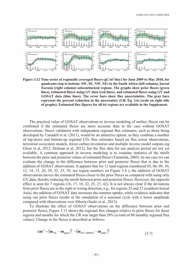
CGER-I143-2019, CGER/NIES
- 93 -
Figure 3.12 Time series of regionally averaged fluxes (gC/m2/day) for June 2009 to May 2010, for quadrants (top to bottom: SW, SE, NW, NE) in the South Africa (left column), boreal Eurasia (right column) subcontinental regions. The graphs show prior fluxes (green lines), estimated fluxes using GV data (red lines), and estimated fluxes using GV and GOSAT data (blue lines). The error bars show flux uncertainties. The gray bars represent the percent reduction in the uncertainty (UR, Eq. 3.6) (scale on right side of graphs). Estimated flux figures for all 64 regions are available in the Supplement.
The practical value of GOSAT observations to inverse modeling of surface fluxes can be
confirmed if the estimated fluxes are more accurate than in the case without GOSAT observations. Direct validation with independent regional flux estimates, such as those being developed by Canadell et al. (2011), would be an attractive option, as they combine a number of top-down and bottom-up regional CO2 flux estimates based on flux tower observations, terrestrial ecosystem models, forest carbon inventories and multiple inverse model outputs (eg Gloor et al, 2012, Dolman et al, 2012), but the flux data for our analysis period are not yet available. A common approach in inverse modeling is to examine statistics of the misfit between the prior and posterior values of estimated fluxes (Tarantola, 2005). In our case we can evaluate the change in the difference between prior and posterior fluxes that is due to the addition of GOSAT observations. It appears that for 12 land regions (numbered 05, 06, 09, 10, 12, 14, 15, 26, 29, 32, 33, 39, see region numbers on Figure 3.4 ), the addition of GOSAT observations moves the estimated fluxes closer to the prior fluxes as compared with using only GV data, thereby reducing the misfit between prior and posterior fluxes. However, the opposite effect is seen for 7 regions (16, 17, 18, 22, 25, 27, 42). It is not always clear if the deviations from prior fluxes are in the right or wrong direction; e.g., for regions 25 and 27 (southern boreal Asia), the addition of GOSAT data increases the summer uptake, while evidence indicates that using our prior fluxes results in the simulation of a seasonal cycle with a lower amplitude compared with observations over Siberia (Saeki et al., 2013).
To illustrate the effect of GOSAT observations on the difference between prior and posterior fluxes, Figure 3.13 shows the regional flux changes relative to prior fluxes for those regions and months for which the UR was larger than 20% (a total of 80 monthly regional flux values). Change in the fluxes is described as follows:
222priorGOSATGVpriorGV mmmmm (3.7)
- 93 -

Chapter 3 Regional CO2 flux estimates for 2009 - 2010 based on GOSAT and ground-based CO2 observations
- 94 -
where GVm is the flux estimated with GV-only observations and GOSATGVm is the flux estimated with GV data combined with GOSAT. A positive value of 2m means the deviation from the prior is reduced (i.e., the estimated flux becomes closer to the prior) and negative 2m indicates that the addition of GOSAT moves the estimated flux away from the prior value. For small changes in fluxes (~1 PgC/year/region) the effect of GOSAT observations is statistically similar for both positive and negative changes. In contrast, a number of large positive 2m values clearly indicate that the addition of GOSAT observations acts to suppress many large and likely erroneous deviations from prior fluxes in the underconstrained regions for which estimations are made with GV data alone.
-10 -8 -6 -4 -2 0 2 4 6 8 100
5
10
15
20
25
num
ber o
f flu
x va
lues
reduction in flux deviation from prior(PgC/region/year)2
Figure 3.13 Change in flux deviation from prior due to addition of the GOSAT observations
expressed as 2m (introduced in Eq. (3.7)) in (PgC/region/year)2 for regions and months where reduction in uncertainty is significant (UR>20%).
As discussed by Gurney et al. (2002, 2004), the problem of unconstrained regions in
inversions is not limited to the large estimated flux uncertainties: the estimated fluxes themselves appear more variable in terms of departure from the prior flux, with a large spread arising when different transport models are used with the same observation data. A reduction in the difference between estimated and prior fluxes for underconstrained regions with the introduction of GOSAT observations would confirm two points. First, a reduction in theoretically estimated flux uncertainty corresponds to a reduction in the deviation of the estimated fluxes themselves from prior fluxes. Second, observations by GOSAT on average do not contradict prior flux estimates; otherwise, the addition of GOSAT observations to the inverse model would increase deviations of the flux estimates from prior, while claiming a reduction in flux uncertainty at the same time.
Estimates of the annual global total flux are another useful test of the validity of results from the inverse model. The global total flux for a 1-year period (June 2009 to May 2010) was estimated to be 4.75 GtC/yr (land/ocean: –2.09/–2.00 GtC/yr) for GV-only data, and 5.18 GtC/yr (land/ocean: –1.19/–2.48 GtC/yr) for GV combined with GOSAT. The fossil fuel emissions for the same period are set as 8.64 GtC/yr, prior flux estimates are (land/ocean): –0.70/–1.71 GtC/yr. Although land–ocean partitioning appears within the range of other model estimates, the difference in global total flux between the two sets of observational data is
Figure 3.13 Change in flux deviation from prior due to addition of the GOSAT observations
expressed as 2mΔ (introduced in Eq. (3.7)) in (PgC/region/year)2 for regions and months where reduction in uncertainty is significant (UR>20%).
- 94 -

CGER-I143-2019, CGER/NIES
- 95 -
indicative of some regional and temporal differences between GOSAT observations and the model-simulated XCO2 distribution based on GV-only data in the inversion. Characterization of the temporal and spatial distribution of the CO2 growth rate for this period (2009–2010) is complicated by high temperatures observed in the Northern Hemisphere during the first half of 2010 (Galarneau et al., 2012), which were followed by a heat wave and a large forest fire in western Russia (Barriopedro et al., 2011; Shvidenko et al., 2011). Further investigations are needed regarding the spatiotemporal variability of the bias in the current XCO2 retrievals. 3.5 Summary and conclusions
We developed a global carbon cycle modeling system designed specifically for analysis of the GOSAT observations of the atmospheric carbon dioxide and producing the estimates of the seasonal and interannual variations of the regional CO2 fluxes. The forward modeling components such as atmospheric transport model, fossil fuel emission inventory, terrestrial biosphere exchange model and the oceanic pCO2 data assimilation system were optimized to match seasonal, interannual and spatial variability of the atmospheric CO2 and surface CO2 fluxes. For accurate simulation of the total CO2 atmospheric column the stratospheric transport is simulated on an isentropic grid and was tuned to reproduce the stratospheric air age. The fossil fuel emission inventory, based on use of large point source data and night lights observations, improved the spatial distribution of CO2 emissions that was confirmed to correlate well with detailed bottom up inventory at the horizontal resolutions of 0.5° to 1°. The terrestrial biospheric model VISIT was optimized to simultaneously fit the observed atmospheric CO2 seasonal cycle, observations of the net primary production and biomass distribution map. Oceanic surface CO2 fluxes were simulated with oceanic 4-D variational data assimilation system based on reanalyzed ocean currents, which uses available pCO2 observations and global oceanic pCO2 climatology as constraints. A recent version of the global fire emission database (GFED) was used to account for fire emissions.
The inverse modeling approach optimizing monthly mean fluxes for 64 regions (Patra et al., 2005b) was extended to utilization of column-averaged observations by GOSAT. The method takes into account vertical profiles of the GOSAT observation sensitivity and the effects of prior CO2 profiles on retrieval provided with column averaging kernel data. A globally constant offset between ground-based in-situ observations and GOSAT retrievals is estimated as optimized parameter. The GOSAT XCO2 data screening is implemented using an observation-adjusted 3-D CO2 concentration climatology. To confirm the consistency between simulated variations of the ground based and total column data, the XCO2 data obtained by inverse model fit to GV data were compared with TCCON observations and good agreement was found.
The inverse modeling system was then applied to analysis of the CO2 observations combining the ground based and aircraft observations available in Globalview database and GOSAT SWIR XCO2 Level 2 ver. 02.00 data. The inverse model fluxes estimated using both GV and GOSAT data appear to be close to those estimated using GV for regions well constrained by GV data. On the other hand, the fluxes change considerably when the data by GOSAT are added for regions remote from GV data, which are accompanied with sizeable estimated flux uncertainty reductions for those regions.
Due to larger number of the observations in present version of XCO2 data (ver. 02.00) and lower scatter higher flux uncertainty reductions for several regions were achieved as compared with previous version (ver. 01.xx) reported by Takagi et al. (2011). Variability of the estimated monthly fluxes was considerably reduced as compared with former version mainly due to
- 95 -

Chapter 3 Regional CO2 flux estimates for 2009 - 2010 based on GOSAT and ground-based CO2 observations
- 96 -
significantly reduced scatter of Level 2 data. For most of the regions and seasons the estimated fluxes fall within a range of natural flux variability estimated with component models. The analysis of the estimated regional flux data and annual mean flux suggests that more improvements in the quantification and correction of the XCO2 Level 2 data biases are desirable. There is a need for a coordinated effort to check and validate the regional monthly CO2 flux estimates. Supplementary information Supplementary information for a corresponding journal paper is available online at a link: http://www.atmos-chem-phys.net/13/9351/2013/acp-13-9351-2013-supplement.zip. Acknowledgements
The GOSAT Project is a joint undertaking of three organizations: the Japan Aerospace Exploration Agency, the National Institute for Environmental Studies (NIES), and the Japanese Ministry of the Environment. The work benefited from support and efforts contributed by P.K. Patra, P. Rayner, T. Nakazawa, G. Inoue, Y. Sasano, H. Akimoto, M. Ikeda, Y. Nakatsuka, Y. Koyama, N. Kadygrov, A. Yaremchuk, M. Naja, H.-S. Kim, T. Machida, Y. Nojiri, T. Shirai, S. Oshchepkov, A. Bril and discussions with H. Mukai, L. Feng, F. Chevallier, S. Houweling, P. Peylin and Transcom project members. Authors would like to thank the members of the GOSAT Project for their contribution to this work. M. Harada, K. Matsubara, and colleagues at Advance Soft Corp. contributed to the development of data processing systems. The NIES supercomputer system (including NEC SX-8R/128M16) was used for the development and implementation of the inverse modeling system components. Globalvew-CO2 dataset used in this study is contributed by cooperating scientists and their organizations. The datasets used for this study were provided by the cooperative research project of the JRA-25/JCDAS long-term reanalysis by Japan Meteorological Agency (JMA) and Central Research Institute of Electric Power Industry (CRIEPI). TCCON data made available to us due to efforts by P. Wennberg, J. Notholt, N. Deutcher, D. Griffith, D. Wunch and a number of contributing scientists. Funding for TCCON is provided by NASA’s Terrestrial Ecology Program (grant NNX11AG01G), the Orbiting Carbon Observatory Program, the Atmospheric CO2 Observations from Space (ACOS) Program, and the Department of Energy/Atmospheric Radiation Measurement (DOE/ARM) Program. We acknowledge funding to support Wollongong site from the Australian Research Council, projects LE0668470, DP0879468, DP110103118 and LP0562346. We acknowledge financial support of the Białystok TCCON site from the Senate of Bremen and EU projects IMECC, GEOMON and InGOS as well as maintenance and logistical work provided by AeroMeteo Service (Białystok) and the RAMCES team at LSCE (Gif-sur-Yvette, France) and additional operational funding from the NIES GOSAT project. RJA was sponsored by U.S. Department of Energy, Office of Science, Biological and Environmental Research (BER) programs and performed at Oak Ridge National Laboratory (ORNL) under U.S. Department of Energy contract DE-AC05-00OR22725.
- 96 -

CGER-I143-2019, CGER/NIES
- 97 -
References
Andres, R. J., Marland, G., Fung, I., Matthews, E. (1996) A 1° × 1° distribution of carbon dioxide emissions from fossil fuel consumption and cement manufacture, 1950–1990. Global Biogeochem. Cy.,10(3), 419–429, doi:10.1029/96GB01523.
Andres, R. J., Marland, G., Fung, I., Matthews, E. (1996) A 1◦ ×1◦ distribution of carbon dioxide emissions from fossil fuel consumption and cement manufacture, 1950–1990. Global Biogeochem. Cy., 10, 419–429.
Andres, R., Gregg, J. S., Losey, L., Marland, G., Boden, T. (2011) Monthly, global emissions of carbon dioxide from fossil fuel consumption. Tellus, 63B, 3,309-327.
Austin, P. M., Houze, Jr., R. A. (1973) A technique for computing vertical transports by precipitating cumuli. J. Atmos. Sci., 30, 1100-1111.
Barriopedro, D., Fischer, E. M., Luterbacher, J., Trigo, R. M., García-Herrera, R. (2011) The hot summer of 2010: Redrawing the temperature record map of Europe. Science, 332, 220-224.
Behringer, D. W., Xue, Y. (2004) Evaluation of the global ocean data assimilation system at NCEP. In: The Pacific Ocean. Eighth symposium on integrated observing and assimilation system for atmosphere, ocean, and land surface, AMS 84th annual meeting, Seattle, Washington, DC, 11–15, 2004.
Belikov, D. A., Maksyutov, S., Miyasaka, T., Saeki, T., Zhuravlev, R., Kiryushov, B. (2011) Mass-conserving tracer transport modelling on a reduced latitude-longitude grid with NIES-TM, Geosci. Model Dev., 4, 207-222.
Belikov, D. A., Maksyutov, S., Sherlock, V., Aoki, S., Deutscher, N. M., Dohe, S., Griffith, D., Kyro, E., Morino, I., Nakazawa, T., et al. (2013a) Simulations of column-average CO2 and CH4 using the NIES TM with a hybrid sigma-isentropic (σ−θ) vertical coordinate. Atmos. Chem. Phys., 13, 1713–1732.
Belikov, D. A., Maksyutov, S., Krol, M., Fraser, A., Rigby, M., Bian, H., Bergmann, D., Bousquet, P., Cameron-Smith, P., Chipperfield, M.P., et al.(2013b) Off-line algorithm for calculation of vertical tracer transport in the troposphere due to deep convection. Atmos. Chem. Phys. Discuss., 13, 1093–1114.
Boden, T. A., Marland, G., Andres, R. J. (2011) Global, Regional, and National Fossil-Fuel CO2 Emissions. Carbon Dioxide Information Analysis Center, Oak Ridge National Laboratory, U.S. Department of Energy, Oak Ridge, Tenn., U.S.A., doi 10.3334/CDIAC/00001_V2011.
Bousquet, B., Peylin, P., Ciais, P., Le Quéré C., Friedlingstein, P., Tans, P. P. (2000) Regional Changes in Carbon Dioxide Fluxes of Land and Oceans Since 1980. Science, 290, 5495, 1342-1346.
Bösch, H., Baker, D., Connor, B., Crisp, D., Miller, C. (2011) Global Characterization of CO2 Column Retrievals from Shortwave-Infrared Satellite Observations of the Orbiting Carbon Observatory-2 Mission. Remote Sens., 3, 270-304.
British Petroleum p.l.c. (2011, 2012) Statistical Review of World Energy. http://www.bp.com/productlanding.do?categoryId=6929&contentId=7044622, last access: Aug 23, 2011, historical data available from www.bp.com/statisticalreview, Last Access Jul 26, 2012)
Bruhwiler, L. M. P., Michalak, A. M., Peters, W., Baker, D. F., Tans, P. (2005) An improved Kalman Smoother for atmospheric inversions. Atmos. Chem. Phys., 5, 2691-2702, doi:10.5194/acp-5- 2691-2005.
Butz, A., Guerlet, S., Hasekamp, O., Schepers, D., Galli, A., Aben, I., Frankenberg, C., Hartmann, J. M., Tran, H., Kuze, A., et al. (2011) Toward accurate CO2 and CH4 observations from GOSAT. Geophys. Res. Lett., 38, L14812, doi:10.1029/2011GL047888.
Canadell J.G., Ciais P., Gurney K., Le Quéré C., Piao S., Raupach M.R., Sabine C.L. (2011) An international effort to quantify regional carbon fluxes. EOS 92, 81-82.
Caspersen, J.P., Pacala, S.W., Jenkins, J.C., Hurtt, G.C., Moorcroft, P.R., Birdsey, R.A. (2000) Contributions of land-use history to carbon accumulation in U.S. forests. Science, 290, 5494, 1148-1151.
Chevallier, F., Maksyutov, S., Bousquet, P., Bréon, F.-M., Saito, R., Yoshida, Y., Yokota, T. (2009) On the accuracy of the CO2 surface fluxes to be estimated from the GOSAT observations. Geophys. Res. Lett., 36, L19807, doi:10.1029/2009GL040108.
Connor, B. J., Bösch, H., Toon, G., Sen, B., Miller, C., Crisp, D. (2008) Orbiting Carbon Observatory: inverse method and prospective error analysis. J. Geophys. Res., 113, D05305.
Dee, D. P., Uppala, S. M., Simmons, A. J., Berrisford, P., Poli, P., Kobayashi, S., Andrae, U., Balmaseda, M. A., Balsamo, G., Bauer, P., et al. (2011) The ERA-Interim reanalysis: configuration and performance of the data assimilation system. Q. J. R. Meteorol. Soc., 137, 553–597.
Deutscher, N. M., Griffith, D. W. T., Bryant, G. W., Wennberg, P. O., Toon, G. C., Washenfelder, R. A., Keppel-Aleks, G., Wunch, D., Yavin, Y., Allen, N. T., et al. (2010) Total column CO2 measurements at Darwin, Australia-site description and calibration against in situ aircraft profiles. Atmos. Meas. Tech., 3, 947-958, doi:10.5194/amt-3-947-2010.
- 97 -

Chapter 3 Regional CO2 flux estimates for 2009 - 2010 based on GOSAT and ground-based CO2 observations
- 98 -
Dolman, A. J., Shvidenko, A., Schepaschenko, D., Ciais, P., Tchebakova, N., Chen, T., van der Molen, M. K., Belelli Marchesini, L., Maximov, T. C., Maksyutov, S., Schulze, E.-D. (2012) An estimate of the terrestrial carbon budget of Russia using inventory based, eddy covariance and inversion methods. Biogeosciences, 9, 5323-5340, doi:10.5194/bg-9-5323-2012.
Elvidge, C. D., Baugh, K. E., Dietz, J. B., Bland, T., Sutton, P. C., Kroehl, H. W. (1999) Radiance calibration of DMSP-OLS low-Light imaging data of human settlements – a new device for portraying the Earth’s surface entire. Remote Sens. Environ., 68, 77-88.
Elvidge, C. D., Ziskin, D., Baugh, K. E., Tuttle, B. T., Ghosh, T., Pack, D. W., Erwin, E. H., Zhizhin, M. (2009) A fifteen year record of global natural gas flaring derived from satellite data. Energies, 2 (3), 595-622.
Fan, S., Gloor, M., Mahlman, J., Pacala, S., Sarmiento, J., Takahashi, T., Tans, P. (1998) A Large terrestrial carbon sink in north America implied by atmospheric and oceanic carbon dioxide data and models. Science, 282, 442-446.
Friedl, M. A., McIver, D. K., Hodges, J. C. F., Zhang, X. Y., Muchoney, D., Strahler, A. H., Woodcock, C. E., Gopal, S., Schneider, A., Cooper, A., et al. (2002) Global land cover mapping from MODIS: algorithms and early results. Remote. Sens. Environ., 83, 287-302.
Fujita, D., Ishizawa, M., Maksyutov, S., Thornton, P., Saeki, T., Nakazawa, T. (2003) Inter-annual Variability of the Atmospheric Carbon Dioxide Concentrations as Simulated with Global Terrestrial Biosphere Models and Atmospheric Transport Model. Tellus-B, 55, 2, 530-546.
Galarneau, T. J., Hamill, T. M., Dole, R. M., Perlwitz, J. (2012) A Multiscale analysis of the extreme weather events over western Russia and northern Pakistan during July 2010. Mon. Wea. Rev., 140, 1639-1664.
Giglio, L., Loboda, T., Roy, D. P., Quayle, B., Justice, C. O. (2009) An active-fire based burned area mapping algorithm for the MODIS sensor, Remote. Sens. Environ., 113, 408-420.
Giglio, L., Randerson, J. T., van der Werf, G. R., Kasibhatla, P. S., Collatz, G. J., Morton, D. C., DeFries, R. S. (2010) Assessing variability and long-term trends in burned area by merging multiple satellite fire products. Biogeosciences, 7, 1171-1186, doi:10.5194/bg-7-1171-2010.
GLOBALVIEW-CO2 (2010) Cooperative Atmospheric Data Integration Project–Carbon Dioxide. on CD-ROM, NOAA ESRL, Boulder, Colorado.
GLOBALVIEW-CO2 (2011) Cooperative Atmospheric Data Integration Project - Carbon Dioxide. on CD-ROM, NOAA ESRL, Boulder, Colorado. [Also available on Internet via anonymous FTP to ftp.cmdl.noaa.gov, Path: ccg/co2/GLOBALVIEW]
Gloor, M., Fan, S.-M., Pacala, S., Sarmiento, J. (2000) Optimal sampling of the atmosphere for purpose of inverse modeling: A model study. Global Biogeochem. Cycles, 14(1), 407-428, doi:10.1029/1999GB900052.
Gloor, M., Gatti, L., Brienen, R., Feldpausch, T. R., Phillips, O. L., Miller, J., Ometto, J. P., Rocha, H., Baker, T., de Jong, B., et al. (2012) The carbon balance of South America: a review of the status, decadal trends and main determinants. Biogeosciences, 9, 5407-5430.
Grant, R. F., Hutyra, L. R., de Oliveira, R. C., Munger, J. W., Saleska, S. R., Wofsy, S.C. (2009) Modelling the carbon balance of Amazonian rainforests: resolving ecological controls on net ecosystem productivity. Ecological Applications, 79(3), 445-463.
Gruber, N., Gloor, M., Fletcher, S. E. M., Doney, S. C., Dutkiewicz, S., Follows, M. J., Gerber, M., Jacobson, A. R., Joos, F., Lindsay, K., et al. (2009) Oceanic sources, sinks and transport of atmospheric CO2. Global Biogeochem. Cycles, 23, GB1005, doi:10.1029/2008GB003349.
Gurney, K. R., Law, R. M., Denning, A. S., Rayner, P. J., Baker, D., Bousquet, P., Bruhwiler, L., Chen, Y.-H., Ciais, P., Fan, S., et al. (2002) Towards robust regional estimates of CO2 sources and sinks using atmospheric transport models. Nature, 415, 626-630.
Gurney, K. R., Law, R. M., Denning, A. S., Rayner, P. J., Baker, D., Bousquet, P., Bruhwiler, L., Chen, Y.-H., Ciais, P., Fan, S., et al.(2003) Transcom 3 CO2 Inversion Intercomparison: 1. Annual mean control results and sensitivity to transport and prior flux information. Tellus, 55B, 2, 555-579.
Gurney, K. R., Law, R. M., Denning, A. S., Rayner, P. J., Pak, B., Transcom-3-L2 modelers (2004) Transcom-3 inversion intercomparison: control results for the estimation of seasonal carbon sources and sinks. Global Biogeochem. Cy., 18, GB1010, doi:10.1029/2003GB002111.
Gurney, K. R., Chen, Y.-H., Maki, T., Kawa, S. R., Andrews, A., Zhu, Z. (2005) Sensitivity of atmospheric CO2 inversions to seasonal and interannual variations in fossil fuel emissions. J. Geophys. Res., 110, D10308, doi:10.1029/2004JD005373.
Gurney, K. R., Mendoza, D., Zhou, Y., Fischer, M., de la Rue du Can, S., Geethakumar, S., Miller, C. C. (2009) The Vulcan Project: High resolution fossil fuel combustion CO2 emissions fluxes for the United States. Environ. Sci. Technol., 43 (14), 5535-5541.
Hack, J. J, Boville, B. A., Briegleb, B. P., Kiehl, J. T., Rasch, P. J., Williamson, D. L. (1993) Description of the NCAR community climate model (CCM2). NCAR/TN-382, 108.
- 98 -

CGER-I143-2019, CGER/NIES
- 99 -
Heimann, M., Keeling, C. (1989) A three-dimensional model of atmospheric CO2 transport based on observed winds: 2: Model description and simulated tracer experiments. Geophys. Mon., 55, 237-275.
Ichii, K., Suzuki, T., Kato, T., Ito, A., Hajima, T., Ueyama, M., Sasai, T., Hirata, R., Saigusa, N., Ohtani, Y., Takagi, K. (2010) Multi-model analysis of terrestrial carbon cycles in Japan: Reducing uncertainties in model outputs among different terrestrial biosphere models using flux observations. Biogeosciences, 7, 2061-2080, doi:10.5194/bg-7-2061-2010.
Ichii, K., Kondo, M., Lee, Y.-H., Wang, S.-Q., Kim, J., Ueyama, M., Lim, H.-J., Shi, H., Suzuki, T., Ito, A., et al. (2013) Site-level model-data synthesis of terrestrial carbon fluxes in the CarboEastAsia eddy-covariance observation network: Toward future modeling efforts. J. For. Res_Jpn., 18, 13–20, doi:10.1007/s10310-012-0367-9.
Ikeda, M., Sasai, Y. (2000) Reconstruction of subsurface DIC and alkalinity fields in the North Pacific using assimilation of upper ocean data. Mar. Chem., 72, 343-358.
Ishii, M., Feely, R. A., Rodgers, K. B., Park, G.–H., Wanninkhof, R., Sasano, D., Sugimoto, H., Nakaoka, S., Telszewski, M., Nojiri, Y., et al. (2014) Air-sea CO2 flux in the Pacific Ocean for the period 1990-2009. Biogeosciences, 11, 709-734, doi: 10.5194/bg-11-709-2014
Ito, A., Oikawa, T. (2002) A simulation model of the carbon cycle in land ecosystems (Sim-CYCLE): A description based on dry-matter production theory and plot-scale validation. Ecol. Model., 151, 147-179.
Ito, A., Sasai, T. (2006) A comparison of simulation results from two terrestrial carbon cycle models using three climate datasets. Tellus, 58B, 513-522.
Ito, A., Ichii, K., Kato, T. (2010) Spatial and temporal patterns of soil respiration over the Japanese Archipelago: A model intercomparison study. Ecological Research, 25, 1033-1044, doi:10.1007/s11284-010-0729-8.
Ito, A. (2010) Changing ecophysiological processes and carbon budget in East Asian ecosystems under near-future changes in climate: Implications for long-term monitoring from a process-based model. J. Plant Res., 123, 577-588.
Jones, P. D., Briffa, K. R. (1992) Global surface air temperature variations during the twentieth century: Part 1, Spatial, Temporal and Seasonal Details. The Holocene, 2, 165-179.
Justice, C. O., Giglio, L., Korontzi, S., Owens, J., Morisette, J. T., Roy, D. P., Descloitres, J., Alleaume, S., Petitcolin, F., Kaufman, Y. (2002) The MODIS fire products. Remote. Sens. Environ., 83, 244-262.
Kadygrov, N., Maksyutov, S., Eguchi, N., Aoki, T., Nakazawa, T., Yokota, T., Inoue, G. (2009) Role of simulated GOSAT total column CO2 observations in surface CO2 flux uncertainty reduction. J. Geophys. Res., 114, D21208.
Keeling, C. D., Whorf, T. P., Wahlen, M., van der Plicht, J. (1995) Interannual extremes in the rate of rise of atmospheric carbon dioxide since 1980. Nature, 375, 666-670.
Kindermann, G. E., McCallum, I., Fritz, S., Obersteiner, M. (2008) A global forest growing stock, biomass and carbon map based on FAO statistics. Silva Fennica, 42, 387-396.
Koyama, Y., Maksyutov, S., Valsala, V. (2009) Model analysis of observational data of the atmospheric tracers for the estimation of greenhouse gases in East Asia. Global Environment Research Account for National Institutes in FY2008, Ministry of the Environment, Japan, 49-95.
Kuze, A., Suto, H., Nakajima, M., Hamazaki, T. (2009) Thermal and near infrared sensor for carbon observation Fourier-transform spectrometer on the Greenhouse Gases Observing Satellite for greenhouse gases monitoring. Appl. Opt., 48, 6716-6733.
McKinley, G. A., Follows, M. J., Marshall, J. (2004) Mechanism of air–sea CO2 ux variability in the equatorial Pacic and North Atlantic. Global Biogeochem. Cy, 18, GB2011, doi:10.1029/2003GB002179.
Maksyutov, S., Patra, P. K., Onishi, R., Saeki, T., and Nakazawa, T. (2008) NIES/FRCGC global atmospheric tracer transport model: description, validation, and surface sources and sinks inversion. J. Earth Simulator, 9, 3-18.
Melillo, J. M., Steudler, P. A., Aber, J. D., Newkirk, K., Lux, H., Bowles, F. P., Catricala, C., Magill, A., Ahrens, T., Morrisseau, S. (2002) Soil Warming and Carbon-Cycle Feedbacks to the Climate System. Science, 298, 2173-2176.
Masarie, K. A., Tans, P. P. (1995) Extension and Integration of Atmospheric Carbon Dioxide Data into a Globally Consistent Measurement Record, J. Geophys. Res., 100, D6, 11593-11610.
Messerschmidt, J., Macatangay, R., Notholt, J., Petri, C., Warneke, T., Weinzierl, C. (2010) Side by side measurements of CO2 by ground-based Fourier transform spectrometry (FTS). Tellus B, 62, 749-758.
Messerschmidt, J., Chen, H., Deutscher, N. M., Gerbig, C., Grupe, P., Katrynski, K., Koch, F.-T., Lavrič, J. V., Notholt, J., Rödenbeck, C., et al. (2011) Automated ground-based remote sensing measurements of greenhouse gases at the Białystok site in comparison with collocated in-situ measurements and model data. Atmos. Chem. Phys. Discuss., 11, 32245-32282.
- 99 -

Chapter 3 Regional CO2 flux estimates for 2009 - 2010 based on GOSAT and ground-based CO2 observations
- 100 -
Monsi, M. and Saeki, T. (1953) Über den Lichtfaktor in den Panzengesellschaften und seine Bedeutung für die Stoffproduktion. Jpn. J. Bot., 14, 22-52.
Morino, I., Uchino, O., Inoue, M., Yoshida, Y., Yokota, T., Wennberg, P. O., Toon, G. C., Wunch, D., Roehl, C. M., Notholt, J., et al. (2011) Preliminary validation of column-averaged volume mixing ratios of carbon dioxide and methane retrieved from GOSAT short-wavelength infrared spectra. Atmos. Meas. Tech., 4, 1061-1076, doi:10.5194/amt-4-1061-2011.
Nakatsuka, Y., Maksyutov, S. (2009) Optimization of the seasonal cycles of simulated CO2 flux by fitting simulated atmospheric CO2 to observed vertical profiles. Biogeosciences, 6, 2733–2741.
Niwa, Y., Patra, P. K., Sawa, Y., Machida, T., Matsueda, H., Belikov, D., Maki, T., Ikegami, M., Imasu, R., Maksyutov, S., et al. (2011) Three-dimensional variations of atmospheric CO2: aircraft measurements and multi-transport model simulations. Atmos. Chem. Phys., 11, 13359-13375.
Oda, T., Maksyutov, S. (2011) A very high-resolution (1km×1 km) global fossil fuel CO2 emission inventory derived using a point source database and satellite observations of nighttime lights. Atmos. Chem. Phys., 11, 543-556.
O'Dell, C. W., Connor, B., Bösch, H., O'Brien, D., Frankenberg, C., Castano, R., Christi, M., Eldering, D., Fisher, B., Gunson, M., et al. (2012) The ACOS CO2 retrieval algorithm – Part 1: Description and validation against synthetic observations. Atmos. Meas. Tech., 5, 99-121, doi:10.5194/amt-5-99-2012.
Ohyama, H., Morino, I., Nagahama, T., Machida, T., Suto, H., Oguma, H., Sawa, Y., Matsueda, H., Sugimoto, N., Nakane, H., Nakagawa, K. (2009) Column-averaged volume mixing ratio of CO2 measured with ground-based Fourier transform spectrometer at Tsukuba. J. Geophys. Res., 114, D18303, doi:10.1029/2008JD011465.
Olson, R. J., Johnson, K. R., Zheng, D. L., Scurlock, J. M. O. (2001) Global and Regional Ecosystem Modeling: Databases of Model Drivers and Validation Measurements. Oak Ridge National Laboratory.
Olsen, S. C., Randerson, J. T. (2004) Differences between surface and column atmospheric CO2 and implications for carbon cycle research. J. Geophys. Res., 109, D02301, doi:10.1029/2003JD003968.
Onogi, K., Tsutsui, J., Koide, H., Sakamoto, M., Kobayashi, S., Hatsushika, H., Matsumoto, T., Yamazaki, N., Kamahori, H., Takahashi, K., et al. (2007) The JRA-25 Reanalysis. J. Meteorol. Soc. Jap., 85, 369-432.
Orr, J. C., Najjar, R., Sabine, C. L., Joos, F. (1999) Abiotic-HOWTO. LSCE/CEA Saclay, Gif-sur-Yvette, France, 25 pp.
Oshchepkov, S., Bril, A., Yokota, T., Morino, I., Yoshida, Y., Matsunaga, T., Belikov, D., Wunch, D., Wennberg, P., Toon, G., et al. (2012) Effects of atmospheric light scattering on spectroscopic observations of greenhouse gases from space: Validation of PPDF-based CO2 retrievals from GOSAT. J. Geophys. Res., 117, D12305.
Pacala, S. W., Hurtt, G., Baker, D., Peylin, P., Houghton, R. A., Birdsey, R. A., Heath, L., Sundquist, E. T., Stallard, R. F., Ciais, P., et al. (2001) Consistent land- and atmosphere-based U.S. carbon sink estimates, Science, 292, 5525, 2316-2320.
Patra, P. K., Ishizawa, M., Maksyutov, S., Nakazawa, T., Inoue, G. (2005a) Role of biomass burning and climate anomalies for land-atmosphere carbon fluxes based on inverse modeling of atmospheric CO2, Global Biogeochem. Cycles, 19, GB3005.
Patra, P. K., Maksyutov, S., Nakazawa, T. (2005b) Analysis of atmospheric CO2 growth rates at Mauna Loa using inverse model derived CO2 fluxes. Tellus, 57B, 357-365.
Patra, P. K., Houweling, S., Krol, M., Bousquet, P., Belikov, D., Bergmann, D., Bian, H., Cameron-Smith, P., Chipperfield, M. P., Corbin, K., et al. (2011) TransCom model simulations of CH4 and related species: linking transport, surface flux and chemical loss with CH4 variability in the troposphere and lower stratosphere. Atmos. Chem. Phys., 11, 12813-12837.
Peters, W., Jacobson, A. R., Sweeney, C., Andrews, A. E., Conway, T. J., Masarie, K., Miller, J. B., Bruhwiler, L. M. P., Petron, G., Hirsch, A. I., et al. (2007) An atmospheric perspective on north American carbon dioxide exchange: CarbonTracker. Proc. Nat. Acad. Sci., 104, 18925-18930.
Piao, S., Fang, J., Ciais, P., Peylin, P., Huang, Y., Sitch, S., Wang, T. (2009) The carbon balance of terrestrial ecosystems in China. Nature, 458, 7241, 1009-1013.
Piao, S. L., Ito, A., Li, S. G., Huang, Y., Ciais, P., Wang, X. H., Peng, S. S., Nan, H. J., Zhao, C., Ahlström, A., et al. (2012) The carbon budget of terrestrial ecosystems in East Asia over the last two decades. Biogeosciences, 9, 3571-3586, doi:10.5194/bg-9-3571-2012.
Rayner, P., Enting, I., Francey, R., Langenfelds, R. (1999) Reconstructing the recent carbon cycle from atmospheric CO2, δ13C and O2/N2 observation. Tellus, 51B, 213-232.
Rayner P. J., O'Brien, D. M. (2001) The utility of remotely sensed CO2 concentration data in surface source inversions. Geophys. Res. Lett., 28, 175-178.
Reuter, M., Bovensmann, H., Buchwitz, M., Burrows, J. P., Connor, B. J., Deutscher, N. M., Griffith, D. W. T., Heymann, J., Keppel‐Aleks, G., Messerschmidt, J., et al. (2011) Retrieval of atmospheric CO2 with
- 100 -

CGER-I143-2019, CGER/NIES
- 101 -
enhanced accuracy and precision from SCIAMACHY: Validation with FTS measurements and comparison with model results. J. Geophys. Res., 116, D04301, doi:10.1029/2010JD015047.
Rödenbeck, C., Houweling, S., Gloor, M., Heimann, M. (2003) CO2 flux history 1982–2001 inferred from atmospheric data using a global inversion of atmospheric transport. Atmos. Chem. Phys., 3, 1919-1964,doi:10.5194/acp-3-1919-2003.
Saeki, T., Maksyutov, S., Sasakawa, M., Machida, T., Arshinov, M., Tans, P., Conway, T. J., Saito, M., Valsala, V., Oda, T., Andres, R. J. (2013) Carbon flux estimation for Siberia by inverse modeling constrained by aircraft and tower CO2 measurements. J. Geophys. Res. Atmos., 118, 1100–1122, doi:10.1002/jgrd.50127.
Saito, M., Ito, A., Maksyutov, S. (2011) Evaluation of biases in JRA-25/JCDAS precipitation and their impact on the global terrestrial carbon balance. J. Climate, 24, 4109-4125.
Saito, M., Ito, A., Maksyutov, S. (2014) Optimization of a prognostic biosphere model for terrestrial biomass and atmospheric CO2 variability. Geosci. Model Dev., 7, 1829-1840, 10.5194/gmd-7-1829-2014.
Saito, R., Houweling, S., Patra, P. K., Belikov, D., Lokupitiya, R., Niwa, Y., Chevallier, F., Saeki, T., Maksyutov, S. (2011) TransCom satellite intercomparison experiment: Construction of a bias corrected atmospheric CO2 climatology. J. Geophys. Res., 116, D21120.
Scurlock, J. M. O., Cramer, W., Olson, R. J., Parton, W. J., Prince, S. D. (1999) Terrestrial NPP: toward a consistent data set for global model evaluation. Ecol. Appl., 9, 913-919.
Shvidenko A. Z., Shchepashchenko, D. G., Vaganov, E. A., Sukhinin, A. I., Maksyutov, S., McCallum, I., Lakyda, I. P. (2011) Impact of Wildfire in Russia between 1998-2010 on Ecosystems and the Global Carbon Budget. Dokl. Earth Sci., 441, 2, 1678-1682.
Stephens, B. B., Gurney, K. R., Tans, P. P., Sweeney, C., Peters, W., Bruhwiler, L., Ciais, P., Ramonet, M., Bousquet, P., Nakazawa, T., et al. (2007) Weak northern and strong tropical land carbon uptake from vertical profiles of atmospheric CO2. Science, 316, 1732-1735.
Takahashi, T., Sutherland, S. C., Sweeney, C., Poisson, A., Metzl, N., Tilbrook, N., Bates, N., Wanninkhof, R., Feely, R. A., Sabine, C., et al. (2002) Global sea–air CO2 flux based on climatological surface ocean pCO2, and seasonal biological and temperature effects. Deep-Sea Res. II, 49, 9–10, 1601-1622.
Takahashi, T., Sutherland, S. C., Wanninkhof, R., Sweeney, C., Feely, R. A., Chipman, D. W., Hales, B., Friederich, G., Chavez, F., Sabine, C., et al. (2009) Climatological mean and decadal changes in surface ocean pCO2 and net sea-air CO2 flux over the global oceans. Deep-Sea Res. II, 56, 554-577.
Takahashi, T., Sutherland, S. C., Kozyr, A. (2011) Global Ocean Surface Water Partial Pressure of CO2 Database: Measurements Performed During 1957-2010 (Version 2010). ORNL/CDIAC-159, NDP-088(V2010), Carbon Dioxide Information Analysis Center, Oak Ridge National Laboratory, U.S. Department of Energy, Oak Ridge, Tennessee, doi: 10.3334/CDIAC/otg.ndp088(V2010).
Takagi H., Saeki, T., Oda, T., Saito, M., Valsala, V., Belikov, D., Saito, R., Yoshida, Y., Morino, I., Uchino, O., et al. (2011) On the benefit of GOSAT observations to the estimation of regional CO2 fluxes. SOLA, 7, 161-164.
Tans, P. P., Fung, I. Y., Takahashi, T. (1990) Observational constrains on the global atmospheric CO2 budget. Science, 247, 1431-1438.
Tarantola, A. (2005) Inverse Problem Theory and Methods for Model Parameter Estimation. Society for Industrial and Applied Mathematics, Philadelphia, USA, 342 pp.
Tiedtke, M. (1989) A comprehensive mass flux scheme for cumulus parameterization in large scale models, Mon. Weather Rev., 117, 1779-1800.
Uchino, O., Kikuchi, N., Sakai, T., Morino, I., Yoshida, Y., Nagai, T., Shimizu, A., Shibata, T., Yamazaki, A., Uchiyama, A., et al. (2012) Influence of aerosols and thin cirrus clouds on the GOSAT-observed CO2: a case study over Tsukuba. Atmos. Chem. Phys., 12, 3393-3404, doi:10.5194/acp-12-3393-2012.
Valsala, V., Maksyutov, S., Ikeda, M. (2008) Design and validation of an offline Oceanic Tracer Transport Model for Carbon Cycle study. J. Climate, 21, 2752-2769.
Valsala, V., Maksyutov, S. (2010) Simulation and assimilation of global ocean pCO2 and air-sea CO2 fluxes using ship observations of surface ocean pCO2 in a simplified biogeochemical offline model. Tellus-B, 62B, 821-840.
Valsala, V., Maksyutov, S., Telszewski, M., Nakaoka, S., Nojiri, Y., Ikeda, M., Murtugudde, R. (2012a) Climate impacts on the structures of the North Pacific air-sea CO2 flux variability. Biogeosciences, 9, 477-492, doi:10.5194/bg-9-477-2012.
Valsala, V., Maksyutov, S., Murtugudde, R. (2012b) A window for carbon uptake in the southern subtropical Indian Ocean. Geophys. Res. Lett., 39, L17605, doi:10.1029/2012GL052857.
Valsala, V., Maksyutov, S. (2013) Interannual variability of the air–sea CO2 flux in the north Indian Ocean. Ocean Dynamics, 63, 165-178, doi:10.1007/s10236-012-0588-7, 1-14.
- 101 -

Chapter 3 Regional CO2 flux estimates for 2009 - 2010 based on GOSAT and ground-based CO2 observations
- 102 -
Valsala, V., Tiwari, Y K., Pillai, P., Roxy, M., Maksyutov, S. (2013) Murtugudde, R.: Intraseasonal variability of terrestrial biospheric CO2 fluxes over India during summer monsoons, J. Geophys. Res., 118(2), 752-769. doi: 10.1002/jgrg.20037.
Vermote, E. F., El Saleous, N. Z., Justice, C. O. (2002) Operational atmospheric correction of the MODIS data in the visible to middle infrared: First results. Remote. Sens. Environ., 83, 97-111.
Washenfelder, R. A., Toon, G. C., Blavier, J.-F., Yang, Z., Allen, N. T., Wennberg, P. O., Vay, S. A., Matross, D. M., Daube, B. C. (2006) Carbon dioxide column abundances at the Wisconsin Tall Tower site. J. Geophys. Res., 111, D22305, doi:10.1029/2006JD007154.
Weaver, C. J., Douglass, A. R., Rood, R. B. (1993) Thermodynamic balance of three-dimensional stratospheric winds derived from a data assimilation procedure. J. Atmos. Sci., 50, 2987-2993.
van der Werf, G. R., Randerson, J. T., Giglio, L., Collatz, G. J., Mu, M., Kasibhatla, P. S., Morton, D. C., DeFries, R. S., Jin, Y., van Leeuwen, T. T. (2010) Global fire emissions and the contribution of deforestation, savanna, forest, agricultural, and peat fires (1997–2009). Atmos. Chem. Phys., 10, 11707-11735.
Wunch, D., Toon, G. C., Blavier, J.-F. L., Washenfelder, R. A., Notholt, J., Connor, B. J., Griffith, D. W. T., Sherlock, V., Wennberg, P. O. (2011a) The Total Carbon Column Observing Network. Phil. Trans. R. Soc. A, 369, 1943, 2087-2112, doi:10.1098/rsta.2010.0240.
Wunch, D., Wennberg, P. O., Toon, G. C., Connor, B. J., Fisher, B., Osterman, G. B., Frankenberg, C., Mandrake, L., O'Dell, C., Ahonen, P., et al. (2011b) A method for evaluating bias in global measurements of CO2 total columns from space. Atmos. Chem. Phys., 11, 12317-12337, doi:10.5194/acp-11-12317-2011.
Yokota, T., Yoshida, Y., Eguchi, N., Ota, Y., Tanaka, T., Watanabe, H., and Maksyutov, S.: Global concentrations of CO2 and CH4 retrieved from GOSAT: First preliminary results. SOLA, 5, 160-163, doi:10.2151/sola.2009-041.
Yoshida, Y., Oguma, H., Morino, I., Suto, H., Kuze, A., Yokota, T. (2009) Mountaintop observation of CO2 absorption spectra using a short wavelength infrared Fourier transform spectrometer. Applied Optics, 49, 71-79.
Yoshida, Y., Ota, Y., Eguchi, N., Kikuchi, N., Nobuta, K., Tran, H., Morino, I., Yokota, T. (2011) Retrieval algorithm for CO2 and CH4 column abundances from short-wavelength infrared spectral observations by the Greenhouse gases observing satellite. Atmos. Meas. Tech., 4, 717-734.
Yoshida, Y., Kikuchi, N., Yokota, T. (2012) On-orbit radiometric calibration of SWIR bands of TANSO-FTS onboard GOSAT. Atmos. Meas. Tech., 5, 2515-2523.
Yoshida, Y., Kikuchi, N., Morino, I., Uchino, O., Oshchepkov, S., Bril, A., Saeki, T., Schutgens, N., Toon, G. C., Wunch, D., et al. (2013) Improvement of the retrieval algorithm for GOSAT SWIR XCO2 and XCH4 and their validation using TCCON data, Atmos. Meas. Tech., 6, 1533-1547, doi:10.5194/amt-6-1533-2013.
Ziskin, D., Baugh, K., Hsu F.C., Ghosh, T., Elvidge, C. (2010) Methods used for the 2006 radiance lights. Proc. 30th Asia-Pacific Advanced Network Meeting, 131-142.
- 102 -

CGER’S SUPERCOMPUTER MONOGRAPH REPORT Vol.25 CGER-I143-2019, CGER/NIES
- 103 -
Chapter 4
Adjoint of the Global Eulerian–Lagrangian Coupled Atmospheric transport model (A-GELCA v1.0): development and validation
This chapter is based on “Belikov, D. A., Maksyutov, S., Yaremchuk, A., Ganshin, A., Kaminski, T., Blessing, S., Sasakawa, M., Gomez-Pelaez, A. J., and Starchenko, A.: Adjoint of the global Eulerian-Lagrangian coupled atmospheric transport model (A-GELCA v1.0): development and validation, Geoscientific Model Development, 9, 749-764, 10.5194/gmd-9-749-2016, 2016”, (c) Authors . Used with permission.
- 103 -

Chapter 4 Adjoint of the Global Eulerian–Lagrangian Coupled Atmospheric transport model
- 104 -
Abstract
We presented the development of the Adjoint of the Global Eulerian–Lagrangian Coupled Atmospheric (A-GELCA) model that consists of the National Institute for Environmental Studies (NIES) model as an Eulerian three-dimensional transport model (TM), and FLEXPART (FLEXible PARTicle dispersion model) as the Lagrangian Particle Dispersion Model (LPDM). The forward tangent linear and adjoint components of the Eulerian model were constructed directly from the original NIES TM code using an automatic differentiation tool known as TAF (Transformation of Algorithms in Fortran; http://www.FastOpt.com), with additional manual pre- and post-processing aimed at improving transparency and clarity of the code and optimizing the performance of the computing, including MPI (Message Passing Interface). The Lagrangian component did not require any code modification, as LPDMs are self-adjoint and track a significant number of particles backwad in time in order to calculate the sensitivity of the observations to the neighboring emission areas. The constructed Eulerian adjoint was coupled with the Lagrangian component at a time boundary in the global domain. The simulations presented in this work were performed using the A-GELCA model in forward and adjoint modes. The forward simulation shows that the coupled model improves reproduction of the seasonal cycle and short-term variability of CO2. Mean bias and standard deviation for five of the six Siberian sites considered decrease roughly by 1 ppm when using the coupled model. The adjoint of the Eulerian model was shown, through several numerical tests, to be very accurate (within machine epsilon with mismatch around to ±6e-14) compared to direct forward sensitivity calculations. The developed adjoint of the coupled model combines the flux conservation and stability of an Eulerian discrete adjoint formulation with the flexibility, accuracy, and high resolution of a Lagrangian backward trajectory formulation. A-GELCA will be incorporated into a variational inversion system designed to optimize surface fluxes of greenhouse gases.
Keywords: atmospheric transport and inverse modeling, adjoint model, carbon cycle
Chapter 4 Adjoint of the Global Eulerian–Lagrangian Coupled Atmospheric transport model (A-GELCA v1.0): development and validation
- 104 -

CGER-I143-2019, CGER/NIES
- 105 -
4.1 Introduction
Forecasts of CO2 levels in the atmosphere and predictions of future climate depend on our scientific understanding of the natural carbon cycle (IPCC, 2007; Peters et al., 2007). To estimate the spatial and temporal distribution of carbon sources and sinks, inverse methods are used to infer carbon fluxes from geographically sparse observations of the atmospheric CO2 mixing ratio (Tans et al., 1989). The first comprehensive efforts in atmospheric CO2 inversions date back to the late 1980s and early 1990s (Enting and Mansbridge, 1989; Tans et al., 1989). With the increase in spatial coverage of CO2 observations and the development of three-dimentional (3-D) tracer transport models, a variety of numerical experiments and projects have been performed by members of the so-called “TransCom” community of inverse modelers (e.g., Law et al., 1996, 2008; Denning et al., 1999; Gurney et al., 2002, 2004; Baker et al., 2006; Patra et al., 2011). A number of studies have proposed improvements to the inverse methods of atmospheric transport, i.e. the efficient computation of the transport matrix by the model adjoint proposed by Kaminski et al. (1999b), use of monthly mean GLOBALVIEW-CO2 ground-based data (current version is for 2014) by Rödenbeck et al. (2003), development of an ensemble data assimilation method by Peters et al. (2005), flux inversion at high temporal (daily) and spatial (model grid) resolution for the first time using continuous CO2 measurements over Europe by Peylin et al. (2005), using satellite data to constrain the inversion of CO2 by Chevallier et al. (2005), and development of a new observational screening technique by Maki et al. (2010). Despite progress in atmospheric CO2 inversions, a recent intercomparison (Peylin et al., 2013) demonstrated the need for further refinement.
In recent decades, the density of the observational network established to monitor greenhouse gases in the atmosphere has been increased, and more measurements taken onboard ships and aircraft are becoming available (Karion et al., 2013; Tohjima et al., 2015). However, on a global scale CO2 observations do not exist for many remote regions not covered by networks. This lack of data is one of the main limitations of atmospheric inversions, which can be filled by monitoring from space (Rayner and O’Brien, 2001). The satellite observation data from current (GOSAT, Kuze et al., 2009; Yokota et al., 2009; OCO-2, Crisp et al., 2004) and future missions (CarbonSat/CarbonSat Constellation; Bovensmann et al., 2010; Buchwitz et al., 2013) offer enormous potential for CO2 inverse modeling. Optimal application of large observed datasets requires expanding the inverse analysis of CO2 to finer resolution, higher precision and faster performance.
To link surface fluxes of CO2 to observed atmospheric concentrations, an accurate model of atmospheric transport and an inverse modeling technique are needed. Generally, the atmospheric constituents transport may be described in two different ways: the Lagrangian and the Eulerian approaches. The Eulerian method treats the atmospheric tracers as a continuum on a control volume basis, so it is more effective at reproducing long-term patterns, i.e. the seasonal cycle or the interhemispheric gradient. Lagrangian Particle Dispersion Models (LPDMs) consider atmospheric tracer as a discrete phase and tracks each individual particle, therefore LPDMs are better for resolving synoptic and hourly variations.
To relate fluxes and concentrations of long-lived species like CO2, a transport model must cover a long simulation period (e.g., Bruhwiler et al., 2005). Therefore, computing time is a critical issue and minimization of the computational cost is essential. For chemically inert tracers, the transport can be represented by a model’s Jacobian matrix, because the simulated concentration at observational sites is a linear function of the flux sets. Theoretically, to compute such matrix the transport model is run multiple times with a set of prescribed surface fluxes. However, this would require an extremely large number of forward model evaluations.
- 105 -

Chapter 4 Adjoint of the Global Eulerian–Lagrangian Coupled Atmospheric transport model
- 106 -
The adjoint of the transport model is an efficient way to accelerate calculation of concentration gradients of the simulated tracer at observational locations (Kaminski et al., 1999). Marchuk (1974) first applied the adjoint approach in atmospheric science. After that, this method became widely used in meteorology. In the 1990s, the use of this approach was expanded to the field of tracer transport modeling (Elbern et al., 1997; Kaminski et al., 1999).
Adjoint models have numerous applications, including the assimilation of concentrations, inverse modeling of chemical source strengths, sensitivity analysis, and parameter sensitivity estimation (Enting, 2002; Haines et al., 2014). Recent studies have used this method to constrain estimates of the emissions of CO2 using retrieved column integrals from the GOSAT satellite (Basu et al., 2013; Deng et al., 2014; Liu et al., 2015).
Using the adjoint model speeds up the process of high dimensional inverse modeling. However, high CPU and memory demands prevent us from using Eulerian chemical transport models (CTMs) with high-resolution grids in inversions. It would be beneficial to increase the model resolution close to observation points, where the strong observation constraint can significantly improve the optimization of the resulting emission fluxes.
LPDM running in the backward mode can explicitly estimate a source–receptor sensitivity matrix by solving the adjoint equations of atmospheric transport (Stohl et al., 2009), which is mathematically presented by a Jacobian expressing the sensitivity of concentration at the observational locations. Marchuk (1995), and Hourdin and Talagrand (2006) provided derivations proving equivalence of the adjoint of forward transport models to backward transport models.
In order to exploit the advantages of both methods, Lagrangian and Eulerian chemical transport models can be coupled to develop an adjoint that is suitable for the simultaneous simulation of contributions from global and regional emissions. Coupling can be performed in several ways; e.g., a regional-scale LPDM can be coupled to a global Eulerian model at a regional domain boundary (Rödenbeck et al., 2009; Rigby et al., 2011), or a global-scale LPDM can be coupled to an Eulerian model at the time boundary (Koyama et al., 2011; Thompson and Stohl, 2014).
The goal of this study is to present the development and evaluation of an Adjoint of the Global Eulerian–Lagrangian Coupled Atmospheric model (A-GELCA), which consists of an Eulerian National Institute for Environmental Studies global Transport Model (NIES-TM; Maksyutov et al., 2008; Belikov et al., 2011, 2013a, 2013b) and a Lagrangian particle dispersion model (FLEXPART; Stohl et al., 2005). This approach utilizes the accurate transport of the LPDM to calculate the signal near to the receptors, and efficient calculation of background responses using the adjoint of the Eulerian global transport model. In contrast to previous works (Rödenbeck et al., 2009; Rigby et al., 2011; Thompson and Stohl, 2014), in which the regional models were coupled at the spatial boundary of the domain, we implemented a coupling at a time boundary in the global model domain (as described in Sect. 4.2.1). A-GELCA can be integrated into a variational inverse modeling system designed to optimize surface fluxes.
The remainder of this paper is organized as follows. An overview of the coupled model is provided in Sect. 4.2. In Sect. 4.3 we describe the variational inversion scheme. In Sect. 4.4 we address several problems regarding the coupled model that have not been covered previously (Ganshin et al., 2012). In Sect. 4.5 we describe the formulation and evaluation of the adjoint model. The computational efficiency of the adjoint model is analyzed in Sect. 4.6, and the conclusions are presented in Sect. 4.7.
Chapter 4 Adjoint of the Global Eulerian–Lagrangian Coupled Atmospheric transport model (A-GELCA v1.0): development and validation
- 106 -

CGER-I143-2019, CGER/NIES
- 107 -
4.2 Model and method 4.2.1 Global coupled Eulerian-Lagrangian model
In this paper we use a global Eulerian-Lagrangian coupled model, the principles of which are described by Ganshin et al. (2012). The coupled model consists of FLEXPART (version 8.0; run in backward mode) as the Lagrangian particle dispersion model, and NIES TM (version NIES-08.1i) as the Eulerian off-line global transport model. For concentration ����� ��� (mole fraction) at receptor point �� and time �� we provide the equation in its discrete form, as implemented in the model for the case of surface fluxes:
,1,1102
IJ
ij
N
n
nijk
IJK
ijk
Bijk
N
n
snij
S
s
sij
CO
airrr fC
NfF
mhNSTmtxC
(4.1)
where i, j, and k are the indices that characterize the location of each grid cell; s is the time index; l
ijF are the surface fluxes in kg⋅m–2⋅s–1; BijkC are the background concentrations
calculated by the Eulerian model at the coupling time; nijkf equals unity if the particle is within
cell i, j, k, otherwise it equals zero; T is the duration of the backward trajectory; S is the number of steps in time; N is the total number of particles; h is the height up to which the effect of the surface fluxes is considered significant; ρ is the average air density below height h; and mair and mCO2 are the molar masses of air and carbon dioxide, respectively. The first term in this formula describes the contribution of the nearby sources of the considered component; these sources are located along the trajectories inside layer h (500 m). The value of the first term is proportional to the flux in each cell along the trajectory, and to the time during which the air particle is inside this cell (Ganshin et al., 2012). The background grid values of the concentrations (calculated by the Eulerian model), which are interpolated to the final points of the backward trajectories, are transferred to the observation point and are the second term in the right-hand side of Eq. (4.1). The FLEXPART model starts simulation at the observation point and calculates seven-day backward trajectories for 1000 air particles, which are dispersed under the influence of turbulent diffusion. The number of particles has been chosen to optimize the computational cost without compromising the quality of modeling by Ganshin et al., (2013). The scheme of concentration calculation for the given location includes coupling of two model approaches. NIES TM calculates global concentrations for the selected time period (usually 1 year to exclude spin-up effect), but stops 7 days before the time of the observations. To obtain the concentrations for the observation time we transport the background concentrations from NIES TM gridbox and contribution from surface sources to the location of observation point along the trajectory ensemble calculated by FLEXPART model (Fig. 4.1). Therefore we have implemented the coupling at a time boundary in the global domain of the NIES transport model, while nested regional modeling systems such as one by Rodenbeck et al (2009) have to couple at both region boundary and time boundary.
- 107 -

Chapter 4 Adjoint of the Global Eulerian–Lagrangian Coupled Atmospheric transport model
- 108 -
Figure 4.1 The computational scheme of the coupled model.
Since the first publication of the GELCA model in 2012, the NIES transport model has undergone significant updates. We provide a brief outline of the major features of the current model. NIES TM is a global three-dimensional CTM that simulates the global distribution of atmospheric tracers between the Earth’s surface and a pressure level of 5 hPa. The model employs the standard horizontal latitude–longitude grid with reduced number of meshes towards the poles and a spatial resolution of 2.5° × 2.5° near the equator(Belikov et al., 2011). The vertical coordinate is a flexible hybrid sigma–isentropic (σ–θ) with 32 levels (Belikov et al., 2013b). To parameterize turbulent diffusivity, we follow the method proposed by Hack et al. (1993), with a separate evaluation of transport processes in the free troposphere and the planetary boundary layer (PBL). The PBL heights are provided by the European Centre for Medium-Range Weather Forecasts (ECMWF) ERA-Interim reanalysis. The modified Kuo-type parameterization scheme is used for cumulus convection (Belikov et al., 2013a).
Inverse modeling assumes that the model reasonably well reproduces the relationship between atmospheric mixing ratio and surface fluxes, assuming that the biases between the simulated and observed concentrations are mostly due to the emission inventories errors. To ensure that this is the case, the NIES TM model has been evaluated extensively. Comparisons against SF6 and CO2 (Belikov et al., 2011, 2013b), CH4 (Patra et al., 2011; Belikov et al., 2013b), and 222Rn (Belikov et al., 2013a) measurements show the model ability to reproduce seasonal variations, interhemispheric gradient and vertical profiles of tracers.
4.2.2 FLEXPART
FLEXPART, like other LPDMs, considers atmospheric tracers as clouds of individual
particles and tracks the pathway of each particle. The advantage of this approach is the direct estimation of the sensitivity of the measurements to the neighboring sinks and sources by tracking the particles backward in time. Usually it is sufficient to simulate for a limited number of days (2-10) to determine where particles intercept the surface layer before they spread vertically and horizontally.
Chapter 4 Adjoint of the Global Eulerian–Lagrangian Coupled Atmospheric transport model (A-GELCA v1.0): development and validation
- 108 -

CGER-I143-2019, CGER/NIES
- 109 -
4.2.3 Meteorological data
To run both models we use reanalysis dataset combining the Japanese 25-yr Reanalysis (JRA-25) and the Japanese Meteorological Agency Climate Data Assimilation System (JCDAS) dataset (Onogi et al., 2007). The JRA-25/JCDAS dataset is distributed on a Gaussian T106 grid with horizontal resolution 1.25° × 1.25°, 40 sigma-pressure levels and in 6-hour time steps. The use of JRA-25/JCDAS data for Eulerian and Lagrangian models provides consistency in the calculated fields; however, some features of FLEXPART and NIES TM require different methods for processing the meteorological data.
4.2.3.1 Meteorological data processing for NIES TM
Isolation of the transport equations is an effective way to save a significant amount of CPU
time during tracer transport simulation. At the preprocessing stage, the NIES TM core produced a static archive of advective, diffusive, and convective mass fluxes with time step similar to the one of the original JRA-25/JCDAS data (6 hour). After that the archive is used by an “offline” model specially designed only for passive transport of tracer. Intermediate fluxes are derived by interpolation.
Besides the mass fluxes, the static archives contain fields of temperature, pressure, humidity, vertical grid parameters (variation of the sigma-isentropic vertical coordinate over time), and others. The pre-calculated and stored data field can be used directly for any of the inert tracers. It is also possible to simulate chemically active tracers if the chemical reaction can be written in the linear decay form; e.g., for 222Rn, CH4. Approximately 20 3-D and 1-dimensional arrays are written to a hard disk for every record. This comprises around 10 GB of data per modelled month for the model’s standard resolution of 2.5° × 2.5°.
4.2.3.2 Meteorological data processing for FLEXPART
Originally, FLEXPART was driven by ECMWF reanalysis dataset distributed on a grid
with regular latitude–longitude horizontal structure and sigma–pressure vertical coordinate. The current version of the model was adapted to use JRA-25/JCDAS data, by horizontal bilinear interpolation of the required parameters from a Gaussian grid to a regular 1.25 × 1.25 grid. The vertical structure and temporal resolution of JRA-25/JCDAS data were used without modification.
Given the large differences in structure, resolution and parameter estimation methods used in different reanalysis dataset, the use of the same meteorology for both Eulerian and Lagrangian models provides significant benefit. 4.3. Inverse modeling for the flux optimization problem
Although the variational inversion method for minimizing the discrepancy between modeled and observed mixing ratios has been well described and published (i.e. Chevallier et al., 2005), we summarize it here.
- 109 -

Chapter 4 Adjoint of the Global Eulerian–Lagrangian Coupled Atmospheric transport model
- 110 -
The aim of the inversion problem is to find the value of a state vector x with n elements that minimizes the cost function J(x):
1 11 1 ,2 2
T Tb bJ x x x B x x Hx y R Hx y (4.2)
where y is a vector of observations with m elements, and the matrix H represents the forward model simulation mapping the state vector x to the observation space. Here, R is the covariance matrix (size m × m) for observational error, which includes instrument and representation errors. The matrix R also includes errors of the forward model H. B is the covariance matrix (size n × n) of error for prior information of the state vector xb. The use of the cost function in the form of Eq. (4.2) assumes that all errors have Gaussian statistics and are unbiased (Rodgers, 2000).
The minimization of the cost function (Eq. 4.2) has an analytic solution that involves a matrix inversion. If the Jacobian H is available this analytic solution can implemented, unless the matrix sizes are too large for the available computing resources. Alternatively, Eq. 4.2 can be solved through an iterative minimization algorithm. In this case, the existence of the gradient of J(x) with respect to x allows using of powerful gradient algorithms for minimization. This gradient is efficiently provided by the adjoint (Giering and Kaminski, 1998; Kaminski et al., 1999; Chevallier et al., 2005).
4.4 Assessment of the coupled model
The effect of different horizontal resolutions on Eulerian models is discussed in detail by Patra et al. (2008). In general, higher resolution helps to resolve a more detailed distribution of the tracer. However, the use of a higher resolution grid leads to additional computational cost, which is not always justified by the resulting model output. Higher resolution does not produce better results largely due to the limited availability of high-resolution meteorology and tracer emission datasets.
The paper by Ganshin et al. (2012) describing the development of the GELCA model provides a model testing report. The advantage of GELCA in reproducing the high-concentration spikes and short-term variations caused mainly by anthropogenic emissions is more vivid when using high resolution (1 km × 1 km) surface fluxes compared to standard resolution (1° × 1°) fluxes. However those tests considered only short 4-month simulations for a limited number of locations.
We expanded the comparison undertaken by Ganshin et al. (2012) to a two-year period using an updated set of prescribed fluxes, which combines four components similar to the analysis performed by Takagi et al. (2011) and Maksyutov et al. (2013): (a) anthropogenic fluxes from the Open source Data Inventory of Anthropogenic CO2 (ODIAC; Oda and Maksyutov, 2011) and the Carbon Dioxide Information Analysis Center’s (CDIAC; Andres et al., 2009, 2011) datasets; (b) biosphere fluxes simulated by the Vegetation Integrative SImulator for Trace gases (VISIT) terrestrial biosphere model (Ito, 2010; Saito et al., 2011, 2013); (c) oceanic fluxes predicted by a data assimilation system based on the Offline ocean Tracer Transport Model (OTTM; Valsala and Maksyutov, 2010); and (d) biomass burning emissions from the Global Fire Emissions Database (GFED) version 3.1 (van der Werf et al., 2010). Biosphere fluxes have daily time step, while the others are monthly. The initial global
Chapter 4 Adjoint of the Global Eulerian–Lagrangian Coupled Atmospheric transport model (A-GELCA v1.0): development and validation
- 110 -

CGER-I143-2019, CGER/NIES
- 111 -
CO2 distribution was obtained from GLOBALVIEW-CO2 (2014). We considered several cases with different model resolutions. For NIES TM we tested
grids at 10.0°, 2.5°, and 1.25° resolutions, with FLEXPART running at 1.0° (Table 4.1). The resolution of the input fluxes was matched to that of FLEXPART. Model results were compared with observations from the World Data Centre for Greenhouse Gases (WDCGG 2015) and the Siberian observations obtained by the Center for Global Environmental Research (CGER) of the National Institute for Environmental Studies (NIES) and the Russian Academy of Science (RAS), from six tower sites (JR-STATION) as described by Sasakawa et al. (2010). The selected site locations are shown in Fig. 4.2.
Table 4.1 The coupled model setups analyzed in this study.
Case Resolution, °
Flux combination NIES TM FLEXPART
Cs-1 10.0 1.0 VISIT + CDIAC + OTTM
Cs-2 2.50 1.0 VISIT + CDIAC + OTTM
Cs-3 1.25 1.0 VISIT + CDIAC + OTTM
Figure 4.2 Map showing the location of the 19 WDCGG sites (red dots, blue labels) and 6 tower
network sites in Siberia (magenta dots, green labels) for which we have performed comparison using forward GELCA simulation.
Figure 4.2 Map showing the location of the 19 WDCGG sites (red dots, blue labels) and 6 tower
network sites in Siberia (magenta dots, green labels) for which we have performed comparison using forward GELCA simulation.
- 111 -

Chapter 4 Adjoint of the Global Eulerian–Lagrangian Coupled Atmospheric transport model
- 112 -
Although the total number of observational stations contributing to the WDCGG is about several hundreds, the set of sites conducting continuous (high temporal resolution is needed for the coupled model) observations is much smaller. We selected 19 sites (Table 4.2). Most of them are concentrated in the temperate latitudes of the northern hemisphere, where the variations in CO2 concentration are most noticeable.
Table 4.2 WDCGG continuous observation sites.
# Identify-
ing code Location Lat., ° Lon.,°
Height
, m
Contributor, contact
person
1 ALT Alert, Canada 82.45 -62.52 210 EC,
Doug Worthy
2 AMS Amsterdam Island, France -37.8 77.53 55 LSCE,
Michel Ramonet
3 AMY Anmyeon-do, Korea 36.53 126.32 47 KMA,
Haeyoung Lee
4 BRW Barrow, USA 71.32 -156.6 11 NOAA/ESRL,
Kirk W Thoning
5 CMN Monte Cimone, Italy 44.18 10.7 2165
IAFMS,
Centro Aeronautica
Militare di Montagna
6 CPT Cape Point, South Africa -34.35 18.48 230 SAWS,
Thumeka Mkololo
7 HUN Hegyhatsal, Hungary 46.95 16.65 248 HMS,
Laszlo Haszpra
8 IZO Izana, Spain 28.3 -16.5 2367 AEMET,
Angel J. Gomez-Pelaez
9 JBN Jubany, Argentina -62.23 -58.67 15 CNR-ICES, DNA-IAA,
Claudio Rafanelli
10 MHD Mace Head, Ireland 53.33 -9.9 8 LSCE,
Michel Ramonet
11 MLO Mauna Loa, USA 19.54 -155.58 3397 NOAA/ESRL,
Kirk W Thoning
12 MNM Minamitorishima, Japan 24.28 153.98 8 JMA, Greenhouse Gas
observation section
13 PAL Pallas-Sammaltunturi,
Finland67.97 24.12 560
FMI,
Juha Hatakka
Chapter 4 Adjoint of the Global Eulerian–Lagrangian Coupled Atmospheric transport model (A-GELCA v1.0): development and validation
- 112 -

CGER-I143-2019, CGER/NIES
- 113 -
14 PRS Plateau Rosa, Italy 45.93 7.7 3480 RSE,
Francesco Apadula
15 PUY Puy de Dome, France 45.77 2.97 1465 LSCE,
Michel Ramonet
16 SSL Schauinsland, Germany 47.92 7.92 1205 UBA,
Karin Uhse
17 WSA Sable Island, Canada 43.93 -60.02 5 EC,
Doug Worthy
18 YON Yonagunijima, Japan 24.47 123.02 30 JMA, Greenhouse Gas
observation section
19 ZEP Zeppelinfjellet, Norway 78.9 11.88 475 ITM,
Birgitta Noone
Here AEMET - Izana Atmospheric Research Center,Meteorological State Agency of Spain; CNR-ICES - International Center for Earth Sciences - CNR, Institute of Acoustics and Sensors; DNA-IAA - Direcion Nacional del Antartico- Istituto Antartico Argentino; EC - Environment Canada; HMS - Hungarian Meteorological Service; IAFMS - Italian Air Force Meteorological Service; ITM - Department of Applied Environmental Science, Stockholm University; JMA - Japan Meteorological Agency; KMA - Korea Meteorological Administration; LSCE - Laboratoire des Sciences du Climat et de l'Environnement; NOAA/ESRL - National Oceanic and Atmospheric Administration/Earth System Research Laboratory; RSE - Ricerca sul Sistema Energetico - RSE S.p.A.; FMI - Finnish Meteorological Institute; SAWS - South African Weather Service; UBA - Federal Environmental Agency Germany.
Siberia is assumed to be a substantial source and sink of CO2, with high uncertainties in the fluxes describing them (McGuire et al., 2009; Hayes et al., 2011; Saeki et al., 2013). As a result, CTMs tend to reproduce the interannual variability of CO2 quite poorly. We selected six tower JR-STATION sites to check the model performance in the Siberian region (Table 4.3).
Table 4.3 Tower network sites in Siberia (JR-STATION).
# Identifying
code Location Lat.,° Lon.,° Height, m
1 DEM Demyanskoe 59.79 70.87 63
2 IGR Igrim 63.19 64.41 47
3 KRS Karasevoe 58.25 82.42 67
4 NOY Noyabrsk 63.43 75.78 43
5 VGN Vaganovo 54.50 62.32 85
6 YAK Yakutsk 62.09 129.36 77
- 113 -

Chapter 4 Adjoint of the Global Eulerian–Lagrangian Coupled Atmospheric transport model
- 114 -
The analyzed sites are divided into three groups. The first group includes remote and marine sites (ALT, AMS, BRW, CPT, IZO, JBN, MLO, MNM, ZEP) with very weak influence of local sources, so the seasonal variation of CO2 is controlled by global, large-scale variations. For these sites contribution by using the Lagrangian component is negligible (see Fig. 4.3-5 panel b to analyze the difference between the coupled and the Eulerian models).
Figure 4.3 a) Correlation coefficients between the CO2 concentrations simulated with the coupled model and those observed, b) difference in correlation coefficients due to the application of the Lagrangian component (positive values mean the results of the coupled model are better than those of the Eulerian model alone) at the selected WDCGG and JR-STATION locations for 2009-2010. The definitions of the cases 1-3 are in Table 4.1
Chapter 4 Adjoint of the Global Eulerian–Lagrangian Coupled Atmospheric transport model (A-GELCA v1.0): development and validation
- 114 -

CGER-I143-2019, CGER/NIES
- 115 -
Figure 4.4 a) Mean bias for the CO2 concentrations simulated with the coupled model, b)
difference in mean bias due to the application of the Lagrangian component (for positive bias – the most usual case – negative values mean the results of the coupled model are better than those of the Eulerian model alone) at the selected WDCGG and JR-STATION locations for 2009-2010. The definitions of the cases 1-3 are in Table 4.1.
- 115 -

Chapter 4 Adjoint of the Global Eulerian–Lagrangian Coupled Atmospheric transport model
- 116 -
Figure 4.5 a) Standard deviation (STD) for the CO2 concentration model-observation mismatch
when using the coupled model, b) difference in STD due to the application of Lagrangian component (negative values mean the results of the coupled model are better than of the Eulerian model alone) at the selected WDCGG and JR-STATION locations for 2009-2010. The definitions of the cases 1-3 are in Table 4.1.
The second group includes sites with domination of long term variability of CO2 and relatively smooth and weak short term variations. Typically, these sites are located on the border of two regions with very different fluxes (AMY, CMN, MHD, PAL, PRS, YON).
The sites selected to the third group are strongly influenced by local emissions and global transport at the same time. Therefore the CO2 concentration variation is controlled by the strength and direction of wind, the depth of the boundary layer and other factors. Such sites are mainly in the northern mid-latitudes (HUN, PUY, SSL, WSA) including all Siberian towers (DEM, IGR, KRS, NOY, VGN, YAK). For these locations contributions of the Eulerian and Lagrangian components are comparable. Therefore, the simulation of CO2 for these sites shows the full potential of the coupled model.
Figures 4.6 compares the coupled and Eulerian model results with observations from the Igrim and Vaganovo towers. The recent modifications indicated in Sect. 4.2.2 have significantly improved the performance of NIES TM compared with the results reported by Ganshin et al. (2012). However, compared to the updated NIES TM the coupled model is better reproducing short term peaks of concentration. This explains the observed reduction of the mean bias and STD (up to 1.5 ppm), and the better simulation of the seasonal variation (in phase and amplitude). Generally, the improvements in the CO2 simulations due to the addition of the Lagrangian component to the Eulerian model are higher than those obtained by increasing the resolution of the Eulerian NIES transport model, as seen for the third group of sites (Fig. 4.3-5).
Chapter 4 Adjoint of the Global Eulerian–Lagrangian Coupled Atmospheric transport model (A-GELCA v1.0): development and validation
Figure 4.5 2 concentration model-observation mismatch
when using the coupled model, b) difference in STD due to the application of Lagrangian component (negative values mean the results of the coupled model are better than of the Eulerian model alone) at the selected WDCGG and JR-STATION locations for 2009-2010. The definitions of the cases 1-3 are in Table 4.1.
a) Standard deviation (STD) for the CO
- 116 -

CGER-I143-2019, CGER/NIES
- 117 -
Figure 4.6 CO2 mixing ratios observed at a) the Igrim and b) Vaganovo towers, and simulated
using the coupled (c) and Eulerian-only (e) models using the setups from Table 4.1 for 2009–2010. Symbols show individual observations; lines depict two-weeks running averages. Here, R, S and M mean the Pearson correlation, standard deviation and mean bias respectively.
a)
b)
Figure 4.6 CO2 mixing ratios observed at a) the Igrim and b) Vaganovo towers, and simulated
using the coupled (c) and Eulerian-only (e) models using the setups from Table 4.1 for 2009–2010. Symbols show individual observations; lines depict two-weeks running averages. Here, R, S and M mean the Pearson correlation, standard deviation and mean bias respectively.
- 117 -

Chapter 4 Adjoint of the Global Eulerian–Lagrangian Coupled Atmospheric transport model
- 118 -
However, improvements in CO2 simulation due to the implementation of the GELCA model were obtained not for all the considered sites. There are several factors that limit the coupled model performance improvement. First, no significant improvement can be expected for the remote and marine sites since they are influenced by very distant emissions and/or nearby homogeneous emissions that are managed appropriately by the Eulerian model. The Lagrangian model introduces very significant improvements for sites influenced by relatively nearby inhomogeneous sources. Second, the use of the very rough Eulerian grid (10.0°) causes a wrong reproduction of the CO2 seasonal cycle due to the large aggregation error, e.g., this happens for ALT and BRW. However, note that such low resolution is used in a rather synthetic case, which is unlikely to be used for actual simulations. Third, temporal irregularities in the observations and noise in the meteorological data bring erroneous signal to the Lagrangian model, causing spurious short term peaks of tracers, which cause degraded results at some locations (e.g., PRS, YAK). This shows that further modification of the setup (i.e. more detailed meteorological data, switch to higher resolution) is necessary. Fourth, the Lagrangian part is very sensitive to the local flux quality. Thus, it is quite problematic to use the highly uncertain surface fluxes to simulate the tracer concentrations and use these concentrations for estimating the quality of different model configurations. However, we cannot improve our analysis, because we do not have concentration measurements for tracers whose surface fluxes are more accurately known, like SF6.
Given the large difference in computational costs running the NIES TM model when using the lower- and the higher-resolution grids (e.g., the computational cost increases by a factor of ~4 between Case 2 and 3), the coupled model is an effective way to improve the CO2 simulation without changing the Eulerian model resolution. 4.5 Construction and validation of the adjoint model 4.5.1 Construction
In this section, we present the development of the adjoint of the coupled model. The incorporation of the Lagrangian component does not require any modification to the code, as LPDMs are self-adjoint. The development of the adjoint of the Eulerian part is more complicated. We decided to develop a discrete adjoint of NIES TM in order to make it consistent with the forward model. An alternative approach is the construction of a continuous adjoint derived from the leading equations of the forward model (Giles and Pierce, 2000). The main advantage of the discrete adjoint model is that the resulting gradients of the numerical cost function are exact, even for nonlinear or iterative algorithms, and this makes easier to validate the adjoint model, which is an essential and complicated task.
The adjoint model for NIES TM was created manually to achieve maximum computational efficiency, while the adjoint of NIES TM to FLEXPART coupler was created using the Transformation of Algorithms in Fortran (TAF) software (http://www.FastOpt.com). However, the use of this tool required some manual treatment of the code. TAF successfully produces the tangent linear and adjoint code of individual procedures, but it gets confused when the model has complex structures (such as loops and conditional operators). Therefore we often manually redesigned and optimized the automatically generated adjoint code to optimize the efficiency, improve readability and clarity of the adjoint model and optimize the performance of computing using MPI, as the TAF code used here (version 1.5) do not fully support MPI routines.
Chapter 4 Adjoint of the Global Eulerian–Lagrangian Coupled Atmospheric transport model (A-GELCA v1.0): development and validation
- 118 -

CGER-I143-2019, CGER/NIES
- 119 -
The advantages of our coupled adjoint model are as follows.
1. Simple incorporation of the Lagrangian part, since no modification of the LPDM is required. Potentially, NIES TM can be coupled to any Lagrangian model.
2. Minimization of the simulation time can be obtained, as once calculated the output from the Lagrangian model is applicable for different long-lived tracers.
3. Reduction of aggregation errors can be achieved, as the sensitivity for small regions and even individual model cells near to observation sites is estimated using the LPDM part, while the sensitivity for large regions remote from the monitoring sites is derived using the Eulerian part (Kaminski et al., 2001).
4. Minimization of the computational cost can be obtained, as high-resolution simulation are performed over a limited number of regions nearby to the observational sites using the LPDM part, while for the rest of the globe the coarse-resolution results are calculated by the Eulerian part.
5. High consistency of the tracer fields calculated by the Lagrangian and the Eulerian models due to the fact that both models use the same input meteorology.
The main drawback of the method is that the deriving of discrete adjoint of Eulerian model
is а significant technical challenge. Another potential drawback is that discrete adjoints of nonlinear advection routines have been shown to have poorer performance for 4D-Var optimization than the continuous adjoints (Liu and Sandu, 2008).
4.5.2 Validation of the coupled adjoint
An essential stage of the adjoint model construction is its validation. A lack of accuracy in the adjoint model will likely degrade the performance of the cost function minimization (Eq. 4.2). Several different tests were carried out to evaluate the accuracy and precision of the constructed adjoint model. Considering the simple formulation of the Lagrangian part, we focused on testing the NIES TM adjoint.
4.5.2.1 Validation of the NIES TM adjoint
The discrete adjoint obtained through automatic differentiation can be easily validated by
comparing the adjoint sensitivities with forward model gradients calculated using the finite difference approximation (Henze at al., 2007).
The forward model sensitivity, λF, is calculated using the one- or two-sided finite difference equation,
�� = �������������� (4.3)
�� = ����������������� (4.4)
- 119 -

Chapter 4 Adjoint of the Global Eulerian–Lagrangian Coupled Atmospheric transport model
- 120 -
where M` denotes the tangent linear model. A range of ε = 0.1–0.01 was proved in most cases to give an optimal balance between truncation and roundoff error (Henze at al., 2007).
In the first test, adjoint simulations were carried out using an initial CO2 distribution, zero surface flux for 2 days (1-2 January 2010) and a horizontal grid with resolution 2.5° × 2.5°. The adjoint gradient was then compared with that from the finite difference calculated using Eq. (4.3). This equation was selected in order to save CPU time by minimizing the number of forward model function calculations. For this test we used ε = 0.01.
To quantify the difference between the two calculations of the sensitivity λ, we define the local relative error
������ ���� = |�����|��� ��
, (4.5)
where the subscripts A and F refer to adjoint and finite difference respectively, whereas lon and lat refer to longitude and latitude, respectively. Figure 4.7c shows E(lon, lat) with a logarithmic color scale. The sensitivities obtained for the adjoint have maximum relative error of order 10−16, indicating that transport in the NIES TM adjoint is correct over short timescales. The overall comparisons did not seriously change if we select different grid cells or use other values of ε.
The definition of the adjoint of the tangent linear forward model M* requires that for an inner product , and two random vectors u and v, the following expression should hold:
��� �� ����� �� = ��� �∗��. (4.6)
For practical use the identity in Eq. (4.6) is rewritten as follows (Wilson et al., 2014):
����u���
�u��∗����u��� = 1. (4.7)
We use Eq. (4.7) to test the adjoint model initialized using several different random random
vectors u and v. For all cases, Eq. (4.7) compares well within machine epsilon with mismatch around to ±6e-14.
Chapter 4 Adjoint of the Global Eulerian–Lagrangian Coupled Atmospheric transport model (A-GELCA v1.0): development and validation
- 120 -

CGER-I143-2019, CGER/NIES
- 121 -
Figure 4.7 Comparison of sensitivities of CO2 concentrations (ppm/(µmol/m2s)) for test 1: (a)
sensitivity calculated considering only the Eulerian adjoint model at a resolution of 2.5°, (b) the same sensitivity calculated directly from NIES forward runs using the one-sided numerical finite difference method with perturbations of ε, and c) the relative difference between derived adjoint and the numerical finite difference gradients. Magenta dots with labels depict the locations and names of the Siberian observation towers.
4.5.2.2 Real case simulation
The next series of calculations was made for real measurements. We used data from the
Siberian observation network (Table 4.3) for the period 1–4 January 2010. CO2 initial conditions and fluxes were the same as those used for the CELGA forward simulations in Section 4.4. We run A-GELCA using grids of 10.0° and 2.5° for Eulerian part and of 1.0° for Lagrangian component (similar to Cs-1 and Cs-2 in Table 4.1) and considered several cases.
The sensitivities of CO2 concentrations were calculated using the Eulerian component only in Figs. 4.8,4.9 a) (resolution of 2.5°), b) (resolution of 10.0°), using the Lagrangian component only in Figs. 4.8,4.9 c)(resolution of 1.0°), and d) (resolution of 1.0°, but aggregated on a grid with resolution of 2.5°), and using the coupled adjoint model in Fig. 4.8,4.9 e) (Eulerian component at a resolution of 2.5° and the Lagrangian component aggregated on the grid with a
Figure 4.7 Comparison of sensitivities of CO2 concentrations (ppm/(µmol/m2s)) for test 1: (a)
sensitivity calculated considering only the Eulerian adjoint model at a resolution of 2.5°, (b) the same sensitivity calculated directly from NIES forward runs using the one-sided numerical finite difference method with perturbations of ε, and c) the relative difference between derived adjoint and the numerical finite difference gradients. Magenta dots with labels depict the locations and names of the Siberian observation towers.
- 121 -

Chapter 4 Adjoint of the Global Eulerian–Lagrangian Coupled Atmospheric transport model
- 122 -
resolution of 2.5°), and f) (as for e) , but the resolution of the Eulerian adjoint model was 10.0°). Figure 4.8 corresponds to the 2-nd day of simulation, while Figure 4.9 is for 4-th day.
Above, we have already stated that the Eulerian part of the coupled model is more effective in reproducing of long-term patterns, while the Lagrangian part is better for resolving synoptic and hourly variations. This follows from the fact that the A-GELCA components have different footprints. The Eulerian adjoint has a wider footprint, with the greatest values in an area where the effect of all stations is summed. The Euler model monitors global and large-scale changes, although some stations can be outside this zone (i.e. YAK, at Fig. 4.8a,g or NOY, at Fig. 4.9a,b). These figures illustrate why the Eulerian model, even with a sufficiently detailed grid, fails to reproduce CO2 variations (Sect. 4.4). The footprint width decreases when the NIES TM resolution is increased, but the value of the sensitivity increases.
The FLEXPART model sensitivity shows more irregular distributions, and higher values closer to the observational sites, thereby reflecting the model's ability to monitor small-scale changes (Fig. 4.8-4.9 panels c,d).
During coupling, the sensitivity is aligned due to the crosslinking of components (Fig. 4.8-4.9 panels e,f). Thus, the intensity has maximum near the stations and smoothly decreases when distance increases. The Eulerian and Lagrangian models employ different approaches and grid resolutions for the modeling of atmospheric tracers, and can thus resolve processes with different time and spatial scales, and underlying physics. By changing the Eulerian model resolution, it is possible to change size of the footprint. This system can utilize responses calculated at higher resolutions, such as 0.5° or 0.1°, but these setups require more accurate driving data and regular observations available for smaller time steps.
Chapter 4 Adjoint of the Global Eulerian–Lagrangian Coupled Atmospheric transport model (A-GELCA v1.0): development and validation
- 122 -

CGER-I143-2019, CGER/NIES
- 123 -
Figure 4.8 Comparison of sensitivities of CO2 concentrations [ppm/(µmol/m2s)] at day 2 (see Sect.
4.5.2.2) calculated using: a) the Eulerian adjoint with a resolution of 2.5°, b) the Eulerian adjoint with a resolution of 10.0°, c) the Lagrangian model on the native model grid with a resolution of 1.0°, d) as for c), but aggregated on the grid with a resolution of 2.5°, e) the coupled adjoint model; results from the Lagrangian adjoint model were aggregated on the grid with a resolution of 2.5°, f) as for e), but the resolution of the Eulerian adjoint model was 10.0°. Note the logarithmic color scale for the plots.
- 123 -

Chapter 4 Adjoint of the Global Eulerian–Lagrangian Coupled Atmospheric transport model
- 124 -
Figure 4.9 As for Fig. 4.8, but for day 4. 4.6 Computational efficiency
We tested several different methods to reduce the computational cost of the adjoint model.
First, the Eulerian part of the adjoint model was driven by static archives of meteorological parameters, as described in Sect. 4.2.4.1. Second, the Lagrangian part of the adjoint model made use of pre-calculated response functions, as described in Sect. 4.2.4.2.
To run the adjoint model we used a Linux workstation with 8 Intel(R) Xeon(R) E5-4650 2.70 GHz processors and 64 GB of RAM. The CPU time of the adjoint model (backward only) was almost equal to CPU time required to run the forward model. It took about 1.3 min for a week-long iteration (forward and backward). The memory demand was about 1 GB. Henze et al. (2007) reports that the ratio between simulation time in backward and forward modes for adjoint models derived for other CTMs, as follows: GEOS-Chem: 1.5, STEM: 1.5, CHIMERE: 3–4, IM-AGES: 4, Polair: 4.5–7, and CIT: 11.75. Thus, the adjoint of the developed coupled model GELCA is quite efficient. To achieve this level of efficiency, a substantial amount of manual programming effort is required, despite the automatic code generated by TAF. The main disadvantage of TAF is that many redundant recomputations are often generated by the compiler. A crucial optimization of the adjoint code is required to eliminate these extra recomputations.
Chapter 4 Adjoint of the Global Eulerian–Lagrangian Coupled Atmospheric transport model (A-GELCA v1.0): development and validation
- 124 -

CGER-I143-2019, CGER/NIES
- 125 -
4.7 Summary
In this paper we have presented the construction and evaluation of an adjoint of the global Eulerian–Lagrangian coupled model GELCA that will be integrated into a variational inverse system designed to optimize surface fluxes. The coupled model combines the NIES three-dimensional transport model as its Eulerian part and the FLEXPART plume diffusion model as its Lagrangian component. The Eulerian and Lagrangian components are coupled at a time boundary in the global domain. The model was originally developed to study the carbon dioxide and methane atmospheric distributions.
The Lagrangian component did not require any code modification, as FLEXPART is a self-adjoint and tracks a significant number of particles backward in time in order to calculate the sensitivity of observations to the neighboring emissions areas.
For Eulerian part, the discrete adjoint was constructed directly from the original NIES TM code, instead of contrasting a continuous adjoint derived from the forward model basic equations. The tangent linear and adjoint models of the NIES TM to FLEXPART coupler were derived using the automatic differentiation software TAF (http://www.FastOpt.com), which significantly accelerated the development. However, considerable manual processing of forward and adjoint model codes was necessary to improve the transparency and clarity of the model and to optimize the computational performance of, including MPI, as the TAF code used here (version 1.5) does not fully support MPI routines.
The main benefit of the developed discrete adjoint is accurate calculation of the numerical cost function gradients, even if the algorithms are nonlinear. The overall advantages of the developed model also include relatively simple incorporation of the Lagrangian part and fast computation using the Lagrangian component, scalability of sensitivity calculation depending on distance to monitoring sites, thereby reducing aggregation errors, and computational efficiency even for high-resolution simulations.
The transport scheme accuracy of the forward coupled model was investigated using the distribution of the atmospheric CO2. The GELCA components and the model itself had previously been validated using various tests and by comparison with measurements and with other transport models for CO2 and other tracers. The analyses in the present paper have shown that CELGA is effective in capturing the seasonal variability of atmospheric tracer at observation sites. Decreasing of the Eulerian model resolution does not significantly distort the transport model performance; however, running the coupled model using NIES TM with low resolution grid can maximize simulation speed and use of data storage.
The Eulerian adjoint was validated using various tests in which the adjoint gradients were compared to gradients calculated with numerical finite difference. We evaluated each routine of the discrete adjoint of the Eulerian model and the adjoint gradients of the cost function. The precision obtained of the results of the considered numerical experiments demonstrates proper construction of the adjoint.
The CPU time needed by the adjoint model is comparable with those of other models, as we used several methods to reduce the computational cost. The forward NIES model was altered so that at each model time step it saved all variables that were also being needed by the adjoint model. These variables therefore did not have to be recalculated for use in the adjoint model. In addition, the adjoint simulation was isolated from the recalculation of NIES TM meteorological parameters and Lagrangian response functions. All supplementary parameters were pre-calculated before running the adjoint and were stored in static archives.
The developed A-GELCA model will be incorporated into a variational inversion system aiming studying greenhouse gases (mainly CH4 and CO2), by assimilating tracer measurements
- 125 -

Chapter 4 Adjoint of the Global Eulerian–Lagrangian Coupled Atmospheric transport model
- 126 -
from in situ, aircraft and remote sensing observations. However, before performing real inverse modeling simulations it is necessary to select a proper minimization program and find the optimal values for the error covariance matrices R and B. Code availability
All code in the current version of the NIES forward model is available on request. Any
potential user interested in these modules should contact D. Belikov ([email protected]) or S. Maksyutov ([email protected]), and any feedback on the modules is welcome. Note that that potential users may need help using the forward and adjoint model effectively, but open support for the model is not available due to lack of resources. The code of the adjoint part of the current NIES model is unavailable for distribution, as it was generated using the commercial tool TAF (http://www.FastOpt.com). However, we can provide the sources which were used as input for TAF.
The FLEXPART code was taken from the official web site http://flexpart.eu/. The procedures necessary to run FLEXPART with the JCDAS reanalysis are also available upon request. Acknowledgments
The authors thank A. Stohl for providing the FLEXPART model. We also thank T.
Machida for Siberian observation data (downloaded from http://db.cger.nies.go.jp/). The JRA-25/JCDAS meteorological datasets used in the simulations were provided by the Japan Meteorological Agency. The WDCGG observation data used in the comparisons were provided by The World Data Centre for Greenhouse Gases. We appreciate cooperation of the WDCGG data providers listed in Table 4.2. The computational resources were provided by NIES. This study was supported by order of the Ministry for Education and Science of the Russian Federation No. 5.628.2014/K, by the Tomsk State University Academic D.I. Mendeleev Fund Program in 2014–2015 and by GRENE Arctic project.
References Andres, R. J., Boden, T. A., Marland, G. (2009) Annual fossil-fuel CO2 emissions: Mass of emissions gridded by
one degree latitude by one degree longitude. Carbon Dioxide Information Analysis Center, Oak Ridge National Laboratory, U.S. Department of Energy, Oak Ridge, Tenn., U.S.A., doi: 10.3334/CDIAC/ffe.ndp058.2009.
Andres, R. J., Gregg, J. S., Losey, L., Marland, G., Boden, T. (2011) Monthly, global emissions of carbon dioxide from fossil fuel consumption, Tellus 63B, 309–327.
Baker, D. F., Law, R. M., Gurney, K. R., Rayner, P., Peylin, P., Denning, A. S., Bousquet, P., Bruhwiler, L., Chen, Y.-H., Ciais, P., et al. (2006) TransCom 3 inversion intercomparison: impact of transport model errors on the interannual variability of regional CO2 fluxes, 1988–2003. Global Biogeochem. Cy., 20, GB1002, doi:10.1029/2004GB002439,.
Basu, S., Guerlet, S., Butz, A., Houweling, S., Hasekamp, O., Aben, I., Krummel, P., Steele, P., Langenfelds, R., Torn, M., et al. (2013) Global CO2 fluxes estimated from GOSAT retrievals of total column CO2. Atmos. Chem. Phys., 13, 8695-8717, doi:10.5194/acp-13-8695-2013.
Belikov, D., Maksyutov, S., Miyasaka, T., Saeki, T., Zhuravlev, R., Kiryushov, B. (2011) Mass-conserving tracer transport modelling on a reduced latitude-longitude grid with NIES-TM, Geosci. Model Dev., 4, 207–222.
Chapter 4 Adjoint of the Global Eulerian–Lagrangian Coupled Atmospheric transport model (A-GELCA v1.0): development and validation
- 126 -

CGER-I143-2019, CGER/NIES
- 127 -
Belikov, D. A., Maksyutov, S., Krol, M., Fraser, A., Rigby, M., Bian, H., Agusti-Panareda, A., Bergmann, D., Bousquet, P., Cameron-Smith, P., et al. (2013a) Off-line algorithm for calculation of vertical tracer transport in the troposphere due to deep convection. Atmos. Chem. Phys., 13, 1093–1114, doi:10.5194/acp-13-1093-2013.
Belikov, D., Maksyutov, S., Sherlock, V., Aoki, S., Deutscher, N. M., Dohe, S., Griffith, D., Kyro, E., Morino, I., Nakazawa, T., et al. (2013b) Simulations of column-average CO2 and CH4 using the NIES TM with a hybrid sigma–isentropic (σ–θ) vertical coordinate. Atmos. Chem. Phys., 13, 1713–1732, doi:10.5194/acp-13-1713-2013.
Bovensmann, H., Burrows, J. P., Buchwitz, M., Frerick, J., Noël, S., Rozanov, V. V., Chance, K. V., Goede, A. P. H. (2010) SCIAMACHY: Mission objectives and measurement modes. J. Atmos. Sci., 56, 127–150.
Bovensmann, H., Buchwitz, M., Burrows, J. P., Reuter, M., Krings, T., Gerilowski, K., Schneising, O., Heymann, J., Tretner, A., Erzinger, J. (2010) A remote sensing technique for global monitoring of power plant CO2 emissions from space and related applications. Atmos. Meas. Tech., 3, 781–811, doi:10.5194/amt-3-781-2010.
Bruhwiler, L. M. P., Michalak, A. M., Peters, W., Baker, D. F., Tans, P. P. (2005) An improved Kalman Smoother for atmospheric inversions. Atmos. Chem. Phys., 5, 2691–2702, doi:10.5194/acp-5- 2691-2005.
Buchwitz, M., Reuter, M., Bovensmann, H., Pillai, D., Heymann, J., Schneising, O., Rozanov, V., Krings, T., Burrows, J. P., Boesch, H., et al. (2013) Carbon Monitoring Satellite (CarbonSat): assessment of atmospheric CO2 and CH4 retrieval errors by error parameterization. Atmos. Meas. Tech., 6, 3477–3500, doi:10.5194/amt-6-3477-2013.
Chevallier, F., Fisher, M., Peylin, P., Serrar, S., Bousquet, P., Bréon, F.-M., Chédin, A., Ciais, P. (2005) Inferring CO2 sources and sinks from satellite observations: method and application to TOVS data. J. Geophys. Res., 110, D24309, doi:10.1029/2005JD006390.
Crisp, D., Atlas, R. M., Bréon, F.-M., Brown, L. R., Burrows, J. P., Ciais, P., Connor, B. J., Doney, S. C., Fung, I. Y., Jacob, D. J., et al. (2004) The Orbiting Carbon Observatory (OCO) mission. Adv. Space Res., 34, 700–709.
Deng, F., Jones, D. B. A., Henze, D. K., Bousserez, N., Bowman, K. W., Fisher, J. B., Nassar, R., O'Dell, C., Wunch, D., Wennberg, P. O., et al. (2014) Inferring regional sources and sinks of atmospheric CO2 from GOSAT XCO2 data. Atmos. Chem. Phys., 14, 3703-3727, doi:10.5194/acp-14-3703-2014.
Elbern, H., Schmidt, H., Ebel, A. (1997) Variational data assimilation for tropospheric chemistry modeling. J. Geophys. Res., 102, 15,967–15,985.
Enting, I. G., Mansbridge, J. V. (1989) Seasonal sources and sinks of atmospheric CO2: Direct inversion of filtered data. Tellus B, 41B, 111–126, doi: 10.1111/j.1600-0889.1989.tb00129.x.
Enting, I. T. (2002) Inverse problems in atmospheric constituent transport. Cambridge University Press, Cambridge, UK.
Ganshin, A., Oda, T., Saito, M., Maksyutov, S., Valsala, V., Andres, R. J., Fisher, R. E., Lowry, D., et al. (2012) A global coupled Eulerian-Lagrangian model and 1 × 1 km CO2 surface flux dataset for high-resolution atmospheric CO2 transport simulations. Geosci. Model Dev., 5, 231–243, doi:10.5194/gmd-5-231-2012.
Giles, M. B., Pierce, N. A. (2000) An Introduction to the Adjoint Approach to Design. Flow Turbul. Combust., 65, 393–415.
Giering, R., T. Kaminski (1998) Recipes for adjoint code construction. Trans. Math. Software, 24(4), 437–474,doi:10.1145/293686.293695.
GLOBALVIEW-CO2 Cooperative Atmospheric Data Integration Project - Carbon Dioxide. on CD-ROM (2014) NOAA ESRL, Boulder, Colorado [Also available on Internet via anonymous FTP to ftp.cmdl.noaa.gov, Path: ccg/co2/GLOBALVIEW].
Gurney, K. R., Law, R. M., Denning, A. S., Rayner, P. J., Baker, D., Bousquet, P., Bruhwilerk, L., Chen, Y.-H., Ciais, P., Fan, S., et al.(2002) Towards robust regional estimates of CO2 sources and sinks using atmospheric transport models. Nature, 415, 626–630.
Gurney, K. R., Law, R. M., Denning, A. S., Rayner, P. J., Pak, B. C., Baker, D., Bousquet, P., Bruhwiler, L., Chen, Y.-H., Ciais, P., et al. (2004) Transcom 3 inversion intercomparison: model mean results for the estimation of seasonal carbon sources and sinks, Global Biogeochem. Cy., 18, GB1010, doi:10.1029/2003GB002111.
Hack, J. J., Boville, B. A., Briegleb, B. P., Kiehl, J. T., Rasch, P. J., Williamson, D. L. (1993) Description of the NCAR community climate model (CCM2), NCAR/TN-382, 108.
Haines, P. E., Esler, J. G., Carver, G. D. (2014) Technical note: Adjoint formulation of the TOMCAT atmospheric scheme in the Eulerian backtracking framework (RETRO-TOM). Atmos. Chem. Phys., 14, 5477–5493.
Hayes, D. J., McGuire, A. D., Kicklighter, D. W., Gurney, K. R., Burnside, T. J., Melillo, J. M. (2011) Is the northern high-latitude land-based CO2 sink weakening?. Global Biogeochem. Cycles, 25, GB3018, doi:10.1029/2010GB003813.
- 127 -

Chapter 4 Adjoint of the Global Eulerian–Lagrangian Coupled Atmospheric transport model
- 128 -
Henze, D. K., Hakami, A., Seinfeld, J. H. (2007) Development of the adjoint of GEOS-Chem. Atmos. Chem. Phys., 7, 2413–2433, doi:10.5194/acp-7-2413-2007.
Hourdin, F., Talagrand, O. (2006) Eulerian backtracking of atmospheric tracers. I: Adjoint derivation and parametrization of subgid-scale transport. Q. J. Roy. Meteor. Soc., 132, 585–603.
IPCC (2007) Climate change 2007: the physical science basis. Contribution of Working Group I to the Fourth Assessment Report of the Intergovernmental Panel on Climate Change, In: Solomon, S., Qin, D., Manning, M., Chen, Z., Marquis, M., et al. (eds.), Cambridge University Press, Cambridge, pp. 135–145.
Ito, A. (2010) Changing ecophysiological processes and carbon budget in East Asian ecosystems under near-future changes in climate: Implications for long-term monitoring from a process-based model. J. Plant Res., 123, 577–588.
Kaminski, T., Heimann, M., Giering, R. (1999a) A coarse grid three-dimensional global inverse model of the atmospheric transport: 1. Adjoint model and Jacobian matrix. J. Geophys. Res., 104(D15), 18,535–18,553, doi:10.1029/1999JD900147.
Kaminski, T., Heimann, M., Giering, R. (1999b) A coarse grid three-dimensional global inverse model of the atmospheric transport: 2. Inversion of the transport of CO2 in the 1980s. J. Geophys. Res., 104(D15), 18,555-18,581, doi:10.1029/1999JD900146.
Kaminski, T., Rayner, P., Heimann, M., Enting, I. (2001) On aggregation errors in atmospheric transport inversions. J. Geophys. Res., 106(D5):4703.
Karion, A., Sweeney, C., Wolter, S., Newberger, T., Chen, H., Andrews, A., Kofler, J., Neff, D., Tans, P. (2013) Long-term greenhouse gas measurements from aircraft. Atmos. Meas. Tech., 6, 511-526, doi:10.5194/amt-6-511-2013.
Koyama, Y., Maksyutov, S., Mukai, H., Thoning, K., Tans, P. (2011) Simulation of variability in atmospheric carbon dioxide using a global coupled Eulerian–Lagrangian transport model. Geosci. Model Dev., 4, 317–324, doi:10.5194/gmd-4-317-2011.
Kuze, A., Suto H., Nakajima M., Hamazaki T. (2009) Thermal and near infrared sensor for carbon observation Fourier-transform spectrometer on the Greenhouse Gases Observing Satellite for greenhouse gases monitoring. Appl. Opt., 48, 6716–6733, doi:10.1364/AO.48.006716.
Law, R. M., Rayner, P. J., Denning, A. S., Erickson, D., Fung, I. Y., Heimann, M., Piper, S. C., Ramonet, M., Taguchi, S., Taylor, J. A., et al. (1996) Variations in modelled atmospheric transport of carbon dioxide and the consequences for CO2 inversions. Global Biogeochem. Cy., 10, 783–796.
Law, R. M., Peters, W., Rödenbeck, C., Aulagnier, C., Baker, I., Bergmann, D. J., Bousquet, P., Brandt, J., Bruhwiler, L., Cameron-Smith, P. J., et al. (2008) TransCom model simulations of hourly atmospheric CO2: Experimental overview and diurnal cycle results for 2002. Global Biogeochem. Cy., 22, GB3009, doi:10.1029/2007GB003050.
Liu, Z. Sandu, A. (2008) On the properties of discrete adjoints of numerical methods for the advection equation. Int. J. Numer. Meth. Fluids, 56: 769–803, doi:10.1002/fld.1547.
Liu, J., Bowman, K. W., Henze D. K. (2015) Source-receptor relationships of column-average CO2 and implications for the impact of observations on flux inversions. J. Geophys. Res. Atmos., 120, 5214–5236, doi: 10.1002/2014JD022914.
Maki, T., Ikegami, M., Fujita, T., Hirahara, T., Yamada, K., Mori, K., Takeuchi, A., Tsutsumi, Y., Suda, K., Conway, T. J. (2010) New technique to analyse global distributions of CO2 concentrations and fluxes from non-processed observational data. Tellus B, 62, 797–809, doi:10.1111/j.1600-0889.2010.00488.x.
Maksyutov, S., Patra, P. K., Onishi, R., Saeki, T., Nakazawa, T. (2008) NIES/FRCGC Global Atmospheric Tracer Transport Model: Description, validation, and surface sources and sinks inversion. J. Earth Simulator, 9, 3–18.
Maksyutov, S., Takagi, H., Valsala, V. K., Saito, M., Oda, T., Saeki, T., Belikov, D. A., Saito, R., Ito, A., Yoshida, Y., Morino, I., et al. (2013) Regional CO2 flux estimates for 2009–2010 based on GOSAT and groundbased CO2 observations. Atmos. Chem. Phys., 13, 9351–9373, doi: 10.5194/acp-13-9351-2013.
Marchuk, G. (1974) Numerical solution of the problems of the dynamics of the atmosphere and the ocean (In Russian). Gidrometeoizdat, Leningrad, 303 pp.
Marchuk, G. I. (1995) Adjoint equations and analysis of complex systems. Series: Mathematics and its applications, v. 295, Kluwer Academic Publishers, Dordrecht and Boston, 484 pp.
McGuire, A. D., Anderson, L. G., Christensen, T. R., Dallimore, S., Guo, L. D., Hayes, D. J., Heimann, M., Lorenson, T. D., Macdonald, R. W., Roulet, N. (2009) Sensitivity of the carbon cycle in the Arctic to climate change. Ecol. Monogr., 79(4), 523–555, doi:10.1890/08-2025.1.
Oda, T., Maksyutov, S. (2011) A very high-resolution (1 km × 1 km) global fossil fuel CO2 emission inventory derived using a point source database and satellite observations of nighttime lights. Atmos. Chem. Phys., 11, 543–556, doi:10.5194/acp-11-543-2011.
Chapter 4 Adjoint of the Global Eulerian–Lagrangian Coupled Atmospheric transport model (A-GELCA v1.0): development and validation
- 128 -

CGER-I143-2019, CGER/NIES
- 129 -
Onogi, K., Tsutsui, J., Koide, H., Sakamoto, M., Kobayashi, S., Hatsushika, H., Matsumoto, T., Yamazaki, N., Kamahori, H., Takahashi, K., et al. (2007) The JRA-25 Reanalysis. J. Meteor. Soc. Japan, 85, 369–432.
Patra, P. K., Law, R. M., Peters, W., Rodenbeck, C., Takigawa, M., Aulagnier, C., Baker, I., Bergmann, D. J., Bousquet, P., Brandt, J., et al. (2008) TransCom model simulations of hourly atmospheric CO2: Analysis of synoptic-scale variations for the period 2002–2003. Global Biogeochem. Cy., 22, GB4013, doi:10.1029/2007GB003081.
Patra, P. K., Houweling, S., Krol, M., Bousquet, P., Belikov, D., Bergmann, D., Bian, H., Cameron-Smith, P., Chipperfield, M. P., Corbin, K., et al. (2011) TransCom model simulations of CH4 and related species: linking transport, surface flux and chemical loss with CH4 variability in the troposphere and lower stratosphere. Atmos. Chem. Phys., 11, 12813–12837, doi:10.5194/acp-11-12813-2011.
Peters, W., Miller, J. B., Whitaker, J., Denning, A. S., Hirsch, A., Krol, M. C., Zupanski, D., Bruhwiler, L., Tans, P. P. (2005) An ensemble data assimilation system to estimate CO2 surface fluxes from atmospheric trace gas observations. J. Geophys. Res., 110, D24304, doi:10.1029/2005JD006157.
Peylin, P., Rayner, P. J., Bousquet, P., Carouge, C., Hourdin, F., Heinrich, P., Ciais, P., AEROCARB contributors (2005) Daily CO2 flux estimates over Europe from continuous atmospheric measurements: 1, inverse methodology. Atmos. Chem. Phys., 5, 3173–3186, doi:10.5194/acp-5-3173-2005.
Peylin, P., Law, R. M., Gurney, K. R., Chevallier, F., Jacobson, A. R., Maki, T., Niwa, Y., Patra, P. K., Peters, W., Rayner, P. J., et al. (2013) Global atmospheric carbon budget: results from an ensemble of atmospheric CO2 inversions. Biogeosciences Discuss., 10, 5301–5360, doi:10.5194/bgd-10-5301-2013.
Rayner P. J., O'Brien, D. M. (2001) The utility of remotely sensed CO2 concentration data in surface source inversions. Geophys. Res. Lett., 28, 175–178.
Rigby, M., Manning, A. J., Prinn, R. G. (2011) Inversion of long-lived trace gas emissions using combined Eulerian and Lagrangian chemical transport models. Atmos. Chem. Phys., 11, 9887–9898, doi:10.5194/acp-11-9887-2011.
Rodgers, C. D. (2000) Inverse methods for atmospheric sounding. vol. 2 of Series on Atmospheric, Oceanic and Planetary Physics, World Scientific, Singapore.
Rödenbeck, C., Houweling, S., Gloor, M., Heimann, M. (2003) CO2 flux history 1982–2001 inferred from atmospheric data using a global inversion of atmospheric transport. Atmos. Chem. Phys., 3, 1919–1964, doi:10.5194/acp-3-1919-2003.
Rödenbeck, C., Gerbig, C., Trusilova, K., Heimann, M. (2009) A two-step scheme for high-resolution regional atmospheric trace gas inversions based on independent models. Atmos. Chem. Phys., 9, 5331–5342, doi:10.5194/acp-9-5331-2009.
Saito, M., Ito, A., Maksyutov, S. (2011) Evaluation of biases in JRA-25/JCDAS precipitation and their impact on the global terrestrial carbon balance. J. Climate, 24, 4109–4125.
Saito, M., Ito, A., Maksyutov, S. (2013) Optimization of a prognostic biosphere model in atmospheric CO2 variability and terrestrial biomass. Geosci. Model Dev. Discuss., 6, 4243–4280, doi:10.5194/gmdd-6-4243-2013.
Saeki, T., Maksyutov, S., Sasakawa, M., Machida, T., Arshinov, M., Tans, P., Conway, T. J., Saito, M., Valsala, V., Oda, T., et al. (2013) Carbon flux estimation for Siberia by inverse modeling constrained by aircraft and tower CO2 measurements. J. Geophys. Res. Atmos., 118, doi:10.1002/jgrd.50127.
Sasakawa, M., K. Shimoyama, T. Machida, N. Tsuda, H. Suto, M. Arshinov, D. Davydov, A. Fofonov, O. Krasnov, T. Saeki, et al. (2010) Continuous measurements of methane from a tower network over Siberia. Tellus 62B, 403–416.
Stohl, A., Forster, C., Frank, A., Seibert, P., Wotawa, G. (2005) Technical note: The Lagrangian particle dispersion model FLEXPART version 6.2. Atmos. Chem. Phys., 5, 2461–2474, doi:10.5194/acp-5-2461-2005.
Stohl, A., Seibert, P., Arduini, J., Eckhardt, S., Fraser, P., Greally, B. R., Lunder, C., Maione, M., Mhle, J., O’Doherty, S., et al. (2009) An analytical inversion method for determining regional and global emissions of greenhouse gases: Sensitivity studies and application to halocarbons. Atmos. Chem. Phys., 9, 1597–1620,doi:10.5194/acp-9-1597-2009.
Takagi, H., Saeki, T., Oda, T., Saito, M., Valsala, V., Belikov, D., Saito, R., Yoshida, Y., Morino, I., Uchino, O., et al. (2011) On the benefit of GOSAT observations to the estimation of regional CO2 fluxes. SOLA, 7, 161–164.
Tans, P. P., Conway, T. J., Nakazawa, T. (1989) Latitudinal distribution of the sources and sinks of atmospheric carbon dioxide derived from surface observations and an atmospheric transport model, J. Geophys. Res., 94, 5151–5172.
Tarantola, A. (2005) Inverse Problem Theory and Methods for Model Parameter Estimation. Society for Industrial and Applied Mathematics, Philadelphia, USA.
- 129 -

Chapter 4 Adjoint of the Global Eulerian–Lagrangian Coupled Atmospheric transport model
- 130 -
Thompson, R. L., Stohl, A. (2014) FLEXINVERT: an atmospheric Bayesian inversion framework for determining surface fluxes of trace species using an optimized grid. Geosci. Model Dev., 7, 2223–2242, doi:10.5194/gmd-7-2223-2014.
Tohjima, Y., Terao, Y., Mukai, H., Machida, T., Nojiri, Y., Maksyutov, S. (2015) ENSO-related variability in latitudinal distribution of annual mean atmospheric potential oxygen (APO) in the equatorial Western Pacific. Tellus B, 67, doi: 10.3402/tellusb.v67.25869.
Valsala V., Maksyutov S. (2010) Simulation and assimilation of global ocean pCO2 and air-sea CO2 fluxes using ship observations of surface ocean pCO2 in a simplified biogeochemical offline model. Tellus-B, 62B, 821–840, doi:10.1111/j.1600-0889.2010.00495.x.
van der Werf, G. R., Randerson, J. T., Giglio, L., Collatz, G. J., Mu, M., Kasibhatla, P. S., Morton, D. C., DeFries, R. S., Jin, Y., van Leeuwen, T. T. (2010) Global fire emissions and the contribution of deforestation, savanna, forest, agricultural, and peat fires (1997–2009). Atmos. Chem. Phys., 10, 11707–11735, doi:10.5194/acp-10-11707-2010.
Wilson, C., Chipperfield, M. P., Gloor, M., Chevallier, F. (2014) Development of a variational flux inversion system (INVICAT v1.0) using the TOMCAT chemical transport model, Geosci. Model Dev., 7, 2485–2500, doi:10.5194/gmd-7-2485-2014, 2014.
WMO World Data Centre for Greenhouse Gases (2015) Introduction to the WMO WDCGG. Japan Meteorological Agency, Tokyo, available at: http://ds.data.jma.go.jp/gmd/wdcgg/introduction.html.
Yokota, T., Yoshida, Y., Eguchi, N., Ota, Y., Tanaka, T., Watanabe, H., Maksyutov, S. (2009) Global concentrations of CO2 and CH4 retrieved from GOSAT: First preliminary results. SOLA, 5, 160–163, doi:10.2151/sola.2009-041.
Chapter 4 Adjoint of the Global Eulerian–Lagrangian Coupled Atmospheric transport model (A-GELCA v1.0): development and validation
- 130 -

CGER’S SUPERCOMPUTER MONOGRAPH REPORT Vol.25 CGER-I143-2019, CGER/NIES
- 131 -
Publications, Authors and Contact person
- 131 -

Publications, Authors and Contact Person
- 132 -
Publications
Belikov DA, Bril A, Maksyutov S, Oshchepkov S, Saeki T, Takagi H, Yoshida Y, et al. (2014)
Column-averaged CO2 concentrations in the subarctic from GOSAT retrievals and NIES transport model simulations. Polar Science 8: 129-145.
Belikov DA, Maksyutov S, Ganshin A, Zhuravlev R, Deutscher NM, Wunch D, Feist DG, et al. (2017) Study of the footprints of short-term variation in XCO2 observed by TCCON sites using NIES and FLEXPART atmospheric transport models. Atmospheric Chemistry and Physics 17: 143-157.
Belikov DA, Maksyutov S, Krol M, Fraser A, Rigby M, Bian H, Agusti-Panareda A, et al. (2013a) Off-line algorithm for calculation of vertical tracer transport in the troposphere due to deep convection. Atmospheric Chemistry and Physics 13: 1093-1114.
Belikov DA, Maksyutov S, Sherlock V, Aoki S, Deutscher NM, Dohe S, Griffith D, et al. (2013b) Simulations of column-averaged CO2 and CH4 using the NIES TM with a hybrid sigma-isentropic (sigma-theta) vertical coordinate. Atmospheric Chemistry and Physics 13: 1713-1732.
Belikov DA, Maksyutov S, Yaremchuk A, Ganshin A, Kaminski T, Blessing S, Sasakawa M, et al. (2016) Adjoint of the global Eulerian-Lagrangian coupled atmospheric transport model (A-GELCA v1.0): development and validation. Geoscientific Model Development 9: 749-764.
Eguchi N, Saito R, Saeki T, Nakatsuka Y, Belikov D, Maksyutov S (2010) A priori covariance estimation for CO2 and CH4 retrievals. Journal of Geophysical Research-Atmospheres 115.
Houweling S, Baker D, Basu S, Boesch H, Butz A, Chevallier F, Deng F, et al. (2015) An intercomparison of inverse models for estimating sources and sinks of CO2 using GOSAT measurements. Journal of Geophysical Research-Atmospheres 120: 5253-5266.
Ishizawa M, Mabuchi K, Shirai T, Inoue M, Morino I, Uchino O, Yoshida Y, et al. (2016a) Inter-annual variability of summertime CO2 exchange in Northern Eurasia inferred from GOSAT XCO2. Environmental Research Letters 11.
Ishizawa M, Uchino O, Morino I, Inoue M, Yoshida Y, Mabuchi K, Shirai T, et al. (2016b) Large XCH4 anomaly in summer 2013 over northeast Asia observed by GOSAT. Atmospheric Chemistry and Physics 16: 9149-9161.
Janardanan R, Maksyutov S, Ito A, Yoshida Y, Matsunaga T (2017) Assessment of Anthropogenic Methane Emissions over Large Regions Based on GOSAT Observations and High Resolution Transport Modeling. Remote Sensing 9.
Janardanan R, Maksyutov S, Oda T, Saito M, Kaiser JW, Ganshin A, Stohl A, et al. (2016) Comparing GOSAT observations of localized CO2 enhancements by large emitters with inventory-based estimates. Geophysical Research Letters 43: 3486-3493.
Kim H-S, Maksyutov S, Glagolev MV, Machida T, Patra PK, Sudo K, Inoue G (2011) Evaluation of methane emissions from West Siberian wetlands based on inverse modeling. Environmental Research Letters 6.
Krol M, de Bruine M, Killaars L, Ouwersloot H, Pozzer A, Yin Y, Chevallier F, et al. (2018) Age of air as a diagnostic for transport timescales in global models. Geoscientific Model Development 11: 3109-3130.
- 132 -

CGER-I143-2019, CGER/NIES
- 133 -
Mabuchi K, Takagi H, Maksyutov S (2016) Relationships between CO2 Flux Estimated by Inverse Analysis and Land Surface Elements in South America and Africa. Journal of the Meteorological Society of Japan 94: 415-430.
Maksyutov S, Takagi H, Valsala VK, Saito M, Oda T, Saeki T, Belikov DA, et al. (2013) Regional CO2 flux estimates for 2009-2010 based on GOSAT and ground-based CO2 observations. Atmospheric Chemistry and Physics 13: 9351-9373.
Maksyutov S., Patra PK, Onishi R, Saeki T, Nakazawa T (2008) NIES/FRCGC global atmospheric tracer transport model: description, validation, and surface sources and sinks inversion. Journal of Earth Simulator 9: 3-18.
Oda T, Maksyutov S (2011) A very high-resolution (1 km x 1 km) global fossil fuel CO2 emission inventory derived using a point source database and satellite observations of nighttime lights. Atmospheric Chemistry and Physics 11: 543-556.
Oda T, Maksyutov S, Andres RJ (2018) The Open-source Data Inventory for Anthropogenic CO2, version 2016 (ODIAC2016): a global monthly fossil fuel CO2 gridded emissions data product for tracer transport simulations and surface flux inversions. Earth System Science Data 10: 87-107.
Patra PK, Houweling S, Krol M, Bousquet P, Belikov D, Bergmann D, Bian H, et al. (2011) TransCom model simulations of CH4 and related species: linking transport, surface flux and chemical loss with CH4 variability in the troposphere and lower stratosphere. Atmospheric Chemistry and Physics 11: 12813-12837.
Saeki T, Maksyutov S, Saito M, Valsala V, Oda T, Andres RJ, Belikov D, et al. (2013a) Inverse Modeling of CO2 Fluxes Using GOSAT Data and Multi-Year Ground-Based Observations. Sola 9: 45-50.
Saeki T, Maksyutov S, Sasakawa M, Machida T, Arshinov M, Tans P, Conway TJ, et al. (2013b) Carbon flux estimation for Siberia by inverse modeling constrained by aircraft and tower CO2 measurements. Journal of Geophysical Research-Atmospheres 118: 1100-1122.
Saeki T, Saito R, Belikov D, Maksyutov S (2013c) Global high-resolution simulations of CO2 and CH4 using a NIES transport model to produce a priori concentrations for use in satellite data retrievals. Geoscientific Model Development 6: 81-100.
Saito M, Ito A, Maksyutov S (2011) Evaluation of Biases in JRA-25/JCDAS Precipitation and Their Impact on the Global Terrestrial Carbon Balance. Journal of Climate 24: 4109-4125.
Saito M, Ito A, Maksyutov S (2014) Optimization of a prognostic biosphere model for terrestrial biomass and atmospheric CO2 variability. Geosci. Model Dev. 7: 1829-1840.
Saito M, Kim H-S, Ito A, Yokota T, Maksyutov S (2016) Enhanced Methane Emissions during Amazonian Drought by Biomass Burning. Plos One 11.
Saunois M, Bousquet P, Poulter B, Peregon A, Ciais P, Canadell JG, Dlugokencky EJ, et al. (2016) The global methane budget 2000-2012. Earth System Science Data 8: 697-751.
Shirai T, Ishizawa M, Zhuravlev R, Ganshin A, Belikov D, Saito M, Oda T, et al. (2017) A decadal inversion of CO2 using the Global Eulerian-Lagrangian Coupled Atmospheric model (GELCA): sensitivity to the ground-based observation network. Tellus Series B-Chemical and Physical Meteorology 69.
Takagi H, Houweling S, Andres RJ, Belikov D, Bril A, Boesch H, Butz A, et al. (2014) Influence of differences in current GOSAT XCO2 retrievals on surface flux estimation. Geophysical Research Letters 41: 2598-2605.
Takagi H, Saeki T, Oda T, Saito M, Valsala V, Belikov D, Saito R, et al. (2011) On the Benefit of GOSAT Observations to the Estimation of Regional CO2 Fluxes. Sola 7: 161-164.
- 133 -

Publications, Authors and Contact Person
- 134 -
Tohjima Y, Kubo M, Minejima C, Mukai H, Tanimoto H, Ganshin A, Maksyutov S, et al. (2014) Temporal changes in the emissions of CH4 and CO from China estimated from CH4/CO2 and CO/CO2 correlations observed at Hateruma Island. Atmospheric Chemistry and Physics 14: 1663-1677.
Thompson RL, Patra PK, Chevallier F, Maksyutov S, Law RM, Ziehn T, van der Laan-Luijkx IT, et al. (2016) Top-down assessment of the Asian carbon budget since the mid 1990s. Nature Communications 7.
Valsala V, Maksyutov S (2010) Simulation and assimilation of global ocean pCO2 and air-sea CO2 fluxes using ship observations of surface ocean pCO2 in a simplified biogeochemical offline model. Tellus Series B-Chemical and Physical Meteorology 62: 821-840.
Valsala V, Maksyutov S, Ikeda M (2008) Design and validation of an offline oceanic tracer transport model for a carbon cycle study. Journal of Climate 21: 2752-2769.
Yokota T, Yoshida Y, Eguchi N, Ota Y, Tanaka T, Watanabe H, Maksyutov S (2009) Global Concentrations of CO2 and CH4 Retrieved from GOSAT: First Preliminary Results. Sola 5: 160-163.
Zhuravlev RV, Ganshin AV, Maksyutov SS, Oshchepkov SL, Khattatov BV (2013) Estimation of global CO2 fluxes using ground-based and satellite (GOSAT) observation data with empirical orthogonal functions. Atmospheric and Oceanic Optics 26: 507-516.
- 134 -

CGER-I143-2019, CGER/NIES
- 135 -
Authors
List of Authors Shamil Maksyutov1, Tomohiro Oda1,2, Makoto Saito1, Hiroshi Takagi1, Dmitry Belikov1,3, Vinu Valsala1,4
1 National Institute for Environmental Studies, Tsukuba, Japan 2 now at Universities Space Research Association /Goddard Space Flight Center, Greenbelt, USA 3 now at Hokkaido University, Sapporo, Japan 4 now at Indian Institute for Tropical Meteorology, Pune, India
Contact person
Shamil Maksyutov Center for Global Environmental Research, National Institute for Environmental Studies 16-2 Onogawa, Tsukuba City, Ibaraki, 305-8506 Japan Tel. 029-850-2212 Fax. 029-850-2219 E-mail: [email protected]
- 135 -

Publications, Authors and Contact Person
- 136 -
- 136 -

- 137 -
CGER’S SUPERCOMPUTER MONOGRAPH REPORT
Vol. 1 CGER-I021-’96 (Out of stock) KOMORI S.: Turbulence Structure and CO2 Transfer at the Air-Sea Interface and Turbulent Diffusion in Thermally-Stratified Flows
Vol. 2 CGER-I022-’96 TOKIOKA T., NODA A., KITOH A., NIKAIDOU Y., NAKAGAWA S., MOTOI T., YUKIMOTO S., TAKATA K.: A Transient CO2 Experiment with the MRI CGCM -Annual Mean Response-
Vol. 3 CGER-I025-’97 NUMAGUTI A., SUGATA S., TAKAHASHI M., NAKAJIMA T., SUMI A.: Study on the Climate System and Mass Transport by a Climate Model
Vol. 4 CGER-I028-’97 (Out of stock) AKIYOSHI H.: Development of a Global 1-D Chemically Radiatively Coupled Model and an Introduction to the Development of a Chemically Coupled General Circulation Model
Vol. 5 CGER-I035-’99 WATANABE M., AMANO K., KOHATA K.: Three-Dimensional Circulation Model Driven by Wind, Density, and Tidal Force for Ecosystem Analysis of Coastal Seas
Vol. 6 CGER-I040-2000 HAYASHI Y.Y., TOYODA E., HOSAKA M., TAKEHIRO S., NAKAJIMA K., ISHIWATARI M.: Tropical Precipitation Patterns in Response to a Local Warm SST Area Placed at the Equator of an Aqua Planet
Vol. 7 CGER-I045-2001 NODA A., YUKIMOTO S., MAEDA S., UCHIYAMA T., SHIBATA K., YAMAKI S.: A New Meteorological Research Institute Coupled GCM (MRI-CGCM2) -Transient Response to Greenhouse Gas and Aerosol Scenarios-
Vol. 8 CGER-I055-2003 (Out of stock) NOZAWA T., EMORI S., NUMAGUTI A., TSUSHIMA Y., TAKEMURA T., NAKAJIMA T., ABE-OUCHI A., KIMOTO M.: Transient Climate Change Simulations in the 21st Century with the CCSR/NIES CGCM under a New Set of IPCC Scenarios
Vol. 9 CGER-I057-2004 MIYAZAKI T., FUJISHIMA S., YAMAMOTO M., WEI Q., HANAZAKI H.: Vortices, Waves and Turbulence in a Rotating Stratified Fluid
Vol. 10 CGER-I060-2005 HAYASHI S., MURAKAMI S., XU K., WATANABE M.: Modeling of Daily Runoff in the Changjiang (Yangtze) River Basin and Its Application to Evaluating the Flood Control Effect of the Three Gorges Project
Vol. 11 CGER-I063-2006 NAKAYAMA T., WATANABE M.: Development of Process-based NICE Model and Simulation of Ecosystem Dynamics in the Catchment of East Asia (Part I)
Vol. 12 CGER-I073-2007 NOZAWA T., NAGASHIMA T., OGURA T., YOKOHATA T., OKADA N., SHIOGAMA H.: Climate Change Simulations with a Coupled Ocean-Atmosphere GCM Called the Model for Interdisciplinary Research on Climate: MIROC
Vol. 13 CGER-I080-2008 SHIBATA K., DEUSHI M.: Simulations of the Stratospheric Circulation and Ozone during the Recent Past (1980-2004) with the MRI Chemistry-Climate Model
- 137 -

- 138 -
Vol. 14 CGER-I083-2008 NAKAYAMA T.: Development of Process-based NICE Model and Simulation of Ecosystem Dynamics in the Catchment of East Asia (Part II)
Vol. 15 CGER-I092-2010 (Out of stock) MAKSYUTOV, S., NAKATSUKA Y., VALSALA V., SAITO M., KADYGROV N., AOKI T., EGUCHI N., HIRATA R., IKEDA M., INOUE G., NAKAZAWA T., ONISHI R., PATRA P.K., RICHARDSON A.D., SAEKI T., YOKOTA T.: Algorithms for Carbon Flux Estimation Using GOSAT Observational Data
Vol. 16 CGER-I097-2011 NAKAJIMA K.: Idealized Numerical Experiments on the Space-time Structure of Cumulus Convection Using a Large-domain Two-dimensional Cumulus-Resolving Model
Vol. 17 CGER-I098-2011 UEDA H.: Atmospheric Motion and Air Quality in East Asia
Vol. 18 CGER-I103-2012 NAKAYAMA T.: Development of Process-based NICE Model and Simulation of Ecosystem Dynamics in the Catchment of East Asia (Part III)
Vol. 19 CGER-I108-2013 KOMORI S.: Numerical Simulations of Turbulence Structure and Scalar Transfer across the Air-Water Interfaces
Vol. 20 CGER-I114-2014 NAKAYAMA T.: Development of Process-based NICE Model and Simulation of Ecosystem Dynamics in the Catchment of East Asia (Part IV)
Vol. 21 CGER-I120-2015 SHIOGAMA H.: Influence of Anthropogenic Aerosol Emissions on Pattern Scaling Projections
Vol. 22 CGER-I127-2016 SATOH M., ROH, W., HASHINO, T.: Evaluations of Clouds and Precipitations in NICAM Using the Joint Simulator for Satellite Sensors
Vol. 23 CGER-I132-2017 GOTO D., SCHUTGENS, N.A.J., OIKAWA, E., TAKEMURA, T., NAKAJIMA, T.: Improvement of a global aerosol transport model through validation and implementation of a data assimilation system
Vol. 24 CGER-I138-2018 TAKEMURA T. AND SPRINTARS DEVELOPER TEAM: Development of a global aerosol climate model SPRINTARS
Vol. 25 CGER-I143-2019 MAKSYUTOV S., ODA T., SAITO M., TAKAGI H., BELIKOV, D., VALSALA, V.: Transport modeling algorithms for application of the GOSAT observations to the global carbon cycle modeling
レポートの多くは、地球環境研究センターのウェブサイトから PDF 形式で閲覧可能です。 http://www.cger.nies.go.jp/ja/activities/supporting/publications/report/index.html Many of the reports are also available as PDF files. See: http://www.cger.nies.go.jp/ja/activities/supporting/publications/report/index.html
- 138 -


Center for Global Environmental Research
National Institute for Environmental Studies, Japan
CG
ER
’S SUPE
RC
OM
PUT
ER
MO
NO
GR
APH
RE
POR
T V
ol.25
CGER-REPORT ISSN 2434-5679CGER-I143-2019
CG
ER-I143-2019
CGER’S SUPERCOMPUTER MONOGRAPH REPORT Vol.25
Transport modeling algorithms for application of the GOSATobservations to the global carbon cycle modeling
Shamil Maksyutov, Tomohiro Oda, Makoto Saito, Hiroshi Takagi, Dmitry Belikov and Vinu Valsala