cgfs publications - dynamics of market liquidity of ... · dynamics of market liquidity of japanese...

Dynamics of market liquidity of Japanese stocks:An analysis of tick-by-tick data of the Tokyo Stock Exchange

Jun Muranaga*

Bank of Japan

Abstract

The purpose of this study is to study dynamic aspects of market liquidity of Japanese stocks. We usetick-by-tick data of the individual stocks listed on the first section of the Tokyo Stock Exchange (TSE)and examine three indicators of market liquidity corresponding to Kyle’s three concepts of marketliquidity: tightness, depth, and resiliency. The first indicator is the bid-ask spread, the differencebetween the best bid and ask prices. The second is market impact, calculated as quote changestriggered by trade execution divided by the corresponding trade volume. And the third is marketresiliency, the convergence speed of the bid-ask spread after trades. We conduct a cross-sectionalanalysis over a sample period from October 2 1995 to September 30 1996 and explore the relationshipbetween trade frequency and the three indicators of market liquidity. The results show that tradefrequency and each of the three indicators are positively correlated. We also analyse the effects of thereduction in tick size (minimal price unit) of the TSE on April 13 1998. We examine variousindicators for 55 days around the reduction and find that the tick size change reduced bid-ask spreadand price volatility and increased trade frequency. These results imply that the reduction in tick sizeimproved market liquidity and efficiency.

* The author thanks Michio Kitahara and Sachiko (Kuroda) Nakada for their assistance. The author also thanks HitoshiMio, Tokiko Shimizu, and Shigenori Shiratsuka for their helpful comments. The views expressed here are those of theauthor and not necessarily those of the Bank of Japan, the Committee on the Global Financial System, or the Bank forInternational Settlements.

1

1. Introduction

Among the various issues concerning market behaviour, this paper focuses on market liquidity.Market liquidity has been considered quite important by those who trade their assets in the market,although its clear definition is yet to be fixed and its quantitative measurement is still premature. Sincemarket liquidity substantially affects the price discovery process in the market, it is supposed to have aclose relationship with market efficiency. Muranaga and Shimizu (1999) explored the significance ofmarket liquidity by considering the relationship between market liquidity and market efficiency orstability.

In finance theory, an efficient market is defined as “a market where all available information isreflected in prices.” According to our definition, a liquid market is “a market where a large tradevolume can be immediately executed with minimum effect on price.” Therefore, by increasing theamount of information that can be deduced from price and by accelerating the speed with whichinformation is reflected in prices, an improvement in market liquidity will enhance the extent to whichavailable information is reflected in market prices, and thus will improve market efficiency. Anincrease in the extent to which information is reflected in prices implies that prices can be determinedmore easily than before and that the price discovery function of the market will operate smoothly.

Stability of the financial market is also a concept closely related to market liquidity. In this paper, wedefine a stable market as “a market where the probability of its price discovery function coming to ahalt is quite small over a sufficiently long period of time.” Destabilisation effects of the market causedby the decline of liquidity will materialise through various processes. In particular, what is worthy ofattention is the possibility that a market can endogenously become unstable when market participantslose confidence in the price discovery function of the market. Such instability will materialise whenmarket participants who try to avoid the risk of a market halt form a majority. This seems to occurwhen price changes and the speed of those changes exceed certain boundary values, and if the markethas insufficient liquidity under normal conditions, it is more likely that sudden shocks will lead to adestabilisation of the market as a whole by the rapid exhaustion of liquidity. Therefore, themaintenance of sufficient liquidity under normal conditions would improve market stabilityautonomously by strengthening the participants’ belief in the market function.

As determinants of market liquidity, market structure elements such as trading rules and variousinstitutional arrangements play an important role.1 In this paper, we conduct an empirical analysisbased on tick-by-tick data of the Tokyo Stock Exchange (TSE). In our analysis, we focus on bid-askspread as a static indicator of market liquidity and market impact and market resiliency as dynamicindicators. As a result, we show that: in understanding the dynamics of market liquidity, we need toanalyse the market with monitoring frequency consistent with trade frequency; and that there is apositive relationship between trade frequency and market liquidity both in static and in dynamic sense.In addition, we conduct an event study on the reduction in tick size (minimal price unit) on the TSE.We investigate the effects of the reduction on the market behaviour and show a possibility that thechange in tick size might reduce implicit trading cost and improve market liquidity and efficiency.

This paper is composed as follows. Following the study of Muranaga and Shimizu (1999), the conceptof market liquidity is defined and indicators of market liquidity are introduced in Section 2. Across-sectional analysis based on tick-by-tick data of Japanese stocks appears in Section 3. Section 4shows an event study on the tick size change in the TSE on 13 April 1998. And finally, Section 5summarises the findings and illustrates issues for future research.

1The research area which studies the effects of market structure on market behavior is called market microstructure theory.For a study which exhaustively reviews past studies of market microstructure, see O’Hara (1995).

2

2. Conceptual summary of market liquidity

2.1 Definition of market liquidity

For an individual market participant, a liquid market is generally defined as a market where a largevolume of trades can be immediately executed with minimum effect on price. From the viewpoint ofthe overall market, market liquidity can be defined, as in Muranaga and Shimizu (1999), as the totalvolume and profile of effective supply and demand. The term “effective supply and demand” refers toeach market participant’s potential trade needs at a certain time which are not necessarily reflected inthe observable order book profile or order flows. The reasons why effective supply and demand do notnecessarily come to the surface include the existence of explicit trading costs such as taxes andtransaction fees, and implicit costs whose magnitude is unknown as a result of the informationasymmetry among market participants.2 New effective supply and demand is induced by explicitdeclines in trading cost and reductions in information asymmetry. In addition, there is anothermechanism by which the information about the price changes caused by trade execution itselfmotivates new transactions and reveals effective demand and supply.

2.2 Measuring market liquidity

The channel by which market liquidity affects the price discovery function of the market has static anddynamic aspects. Past studies of market liquidity have mainly focused on the static aspects and haveadopted indicators which show static market depth, such as turnover and bid-ask spread, as measuresof market liquidity. Observability in the market was an important factor in selecting such indicators forthe sake of analysis. In the following, taking into account the market liquidity indicators proposed inthe past studies, we take the TSE as an example and consider possible indicators for measuring marketliquidity from available data.

According to Kyle (1985), market liquidity is represented by the three concepts of tightness, depth,and resiliency. Figure 1 illustrates the relationship between these three concepts summarised by Engleand Lange (1997). Tightness shows the difference between trade price and actual price, and is usuallymeasured as the bid-ask spread. Depth shows the volume which can be traded at current price level,3

and Resiliency is shown by the speed of convergence from the price level which has been brought byrandom price changes. In Figure 1, the best ask price is assumed to move up by a trade execution attime t. Since the market has a tendency to restore the condition, the best ask price will come downwith a new limit order at time t+1. The convergence speed of bid-ask spread could be interpreted asresiliency of the market.

2Explicit costs refer to costs which are clearly known by the market participants before they trade, while implicit costsrefer to those whose amounts are uncertain before the trade due to factors such as information asymmetry. This is aclassification from the viewpoint of a market participant who only has only partial market information, and once he orshe has complete market information, implicit costs will become zero and only explicit costs will remain.

3There are various definitions about market depth and market resiliency. For example, Kyle’s definition of depth isdifferent from that of Muranaga and Shimizu (1999) in that the former does not take into account of potential trade needs(effective supply and demand). In the following, we adopt Kyle’s definition of market depth considering its facility ofobserving and estimating in empirical analysis.

3

Figure 1. Three concepts of market liquidity

limit sellorders

limit buyorders

volume oflimit sell orders

tightness

depth

resiliency(convergence speed)

price of limit orders

volume oflimit buy orders

best bid price

best ask price at t

best ask price at t+1

Muranaga and Shimizu (1999) argue that, in order to examine how market liquidity affects the pricediscovery function in an actual market, not only the static aspects of market liquidity but also thedynamic aspects should be taken into account. In other words, since effective supply and demand canonly be recognised during the dynamic process of trade execution, we need to observe dynamicindicators such as price changes upon trade execution (market impact) and/or the convergence speedof the bid-ask spread (market resiliency). These dynamic indicators reflect the actual results of theexecution of a transaction and the process by which information derived from such results is digestedin the market. Especially when discussing market liquidity under stress, which has a close relationshipwith market stability, it becomes essential to analyse such dynamic indicators as well as staticindicators. In the following, what each indicators stand for is summarised.

First, turnover, or the number of trades, the most simple market liquidity indicator widely used to date,shows the volume or the number of trades which have been executed from among the trade ordersexplicitly placed in the market during a specified observation period, and refers to the tradable volumeor number of trades in the market from a historical viewpoint. Therefore, these indicators neitherreflect the state of effective supply and demand nor trade orders which were not executed despitehaving been explicitly placed in the market. From the viewpoint of time dimension, they do representthe market conditions of a certain period in the past. Although they do not provide timely informationabout the condition of market liquidity, such as “how much of a shock will there be if one executes atrade right now,” they could include a piece of information which is needed for market participantswho are about to execute a trade.

Second, we turn to the bid-ask spread, a static indicator, although it is the one which has been mostwidely used in recent studies on market liquidity. The bid-ask spread corresponds to tightness inKyle’s definition, and, time dimension-wise, the bid-ask spread provides better information aboutmarket liquidity than turnover and the number of trades in that it shows how much the cost will be inthe case of an immediate transaction. However, the bid-ask spread only expresses the transaction costfor those who wish to execute a marginal trade in the market, and does not provide information abouthow many units will be absorbed (depth of order book) or about the extent to which a price will moveafter limit orders at the best quoted price have been digested (price continuity of order book). Suchinformation can be gathered from the dynamic indicators which we plan to employ in this paper.

4

Market impact ( λ ) is a dynamic market liquidity indicator, providing information about the ability ofthe market to absorb trades as changes in price which take place upon trade execution. λ is anindicator which shows to what extent the bid-ask spread will be widened upon execution of a newtrade, and it is measured as the ratio of price impact to trade volume standardised by the “normalmarket size.4” Normal market size is a measure which is represented by the total volume of the orderbook at a certain time. λ provides information about the order book-profile which is standardised bythe normal market size. Although, from the viewpoint of time dimension, currently observableλ represents historical trade executions, it also includes forward-looking information about pricechanges resulting from future transactions and thus will be able to serve as useful measure of marketliquidity in case the availability of current order book information improves.

sizemarket normal volumetrade

change pricebid/ask of ratio)(impactmarket =λ

Another dynamic indicator by which to measure market liquidity is market resiliency (γ ). Thismeasure provides information about potential trade needs (effective supply and demand) which is notexplicitly placed in the market as an order. How to measure γ is yet to be clarified, althoughmeasuring an indicator which shows how the market autonomously restores its original state after acertain shock (trade execution) has been added to the market may be a way to measure γ . In physics,the restoration speed of a coil, for example, is measured as an indicator of resiliency. As an analogy,by measuring the widened bid-ask spread caused by trade executions and the period of time requiredfor the spread to be restored to the state existing immediately before the execution, we can calculatethe restoration speed, and be able to recognise market resiliency. This method captures the process bywhich trade needs, which was potential immediately before the trade execution, materialises upontrade execution, and enables us to measure market liquidity, taking into account potential trade needs.However, we should note that, in an actual market, γ may not be observable at every trade since newmarket orders could well be placed before the bid-ask spread has been restored by new limit orders.By taking into account such market orders occurring during the spread restoration period, the conceptof market resiliency can come close to being an observable liquidity indicator.

market resiliencyratio of bid / ask price change

restoration time of bid ask spread( )γ =

−

3. Cross-sectional analysis

3.1 Data profile

This Section provides a cross-sectional analysis based on tick-by-tick data of the stocks listed in thefirst section of the TSE.5 The data observation period is one year, ranging from October 2 1995 toSeptember 30 1996. The format of the raw data file is shown in Figure 2. Each column shows, fromthe left, security code, time stamp, trade execution price, trade volume, best-bid price, best-ask price,flag of best-bid, and flag of best-bid. The flag of bid/ask will take the form of 0 (trade volumeinformation and has no relation to bid or ask), 1 (warning indication), 2 (normal indication), 3 (marketindication), and 4 (special indication).6

4 In this paper, we standardise trade volume using normal market size in order to focus on price continuity of order book

rather than depth of order book. This adjustment seems useful in cross-sectional analyses of market impact.

5The data are provided on magnetic tape from the Nikko Securities Co., Ltd. for the purpose of this research.

6 Waning and special indications are quoted when the market faces decrease in liquidity. On August 24 1998, the TSE stop

quoting warning indication and ease the standard for special indication in order to increase continuity of price discovery.

5

Figure 2. Format of raw data file

AAAA 1331 100 10000 0 0 0 0

AAAA 1331 0 0 98 100 2 2

BBBB 1331 1020 2000 0 0 0 0

BBBB 1331 0 0 1020 1030 2 2

CCCC 1332 891 6500 0 0 0 0

CCCC 1332 0 0 889 891 2 2

· · · · · · · ·

· · · · · · · ·

· · · · · · · ·

When using tick-by-tick data of the TSE, one should be aware of the following two technical features:

• There are cases when a quote (best-bid or best-ask) does not exist; and

• There is a shutdown system which halts trade execution with quoting warning indication orspecial indication.

These features are unique to the TSE, which has adopted a continuous auction system, a system inwhich an exchange-designated specialist or market maker does not exist.7 In order to avoid the firstproblem, we select issues which have relatively high liquidity and constant quotes. The phenomenonthat a quote for low liquidity issues disappears is indeed important and interesting topic to explore,although, in order to gain foothold in tackling such a topic, we consider it beneficial to clarify andsummarise the facts about issues which are constantly quoted. Since Lehman et al (1994) concludedthat the effects of the existence of warning/special indication on actual price formation are notsignificant,8 we do not make a special treatment in this paper of the second problem. In addition, if weconfine our analysis to issues with relatively high liquidity, we can avoid a considerable extent of thesecond problem.

Based on the above consideration, we picked data regarding the individual issues included in theTOPIX Electrical Machinery Index among those listed in the first section of the TSE. By analysingsuch issues, which have relatively high liquidity and are included in the same industry, we can avoidthe problem of quote disappearance and reduce the effects of noise inherent in individual issues. As ofend-February 1998, the TOPIX Electrical Machinery Index is composed of 133 issues. Of those

7TSE carries members called exchange-designated saitori. Saitori members will match trade orders of member securityfirms and offer quotations such as warning and special quotations in the face of market liquidity decline, although theyare prohibited from self-dealing and thus do not provide liquidity by themselves.

8As specific factors, they have pointed out that (1) range of indications and restrictions on price fluctuations are as large asone to two percentage points on average, and (2) since indication terminates upon execution of even one trade, actualperiod of the indication to be on screen will not be so long (less than 2 minutes in 80% of all cases).

6

issues, 108 issues have been included in the Index and were traded through electronic trading9 duringthe data observation period of October 2 1995 to September 30 1996. We have adopted these108 issues for our analysis, only except measurement of market impact. In measuring market impactwe used 102 issues by excluding 6 from these 108 issues which had a quote disappearance period ofmore than half of the observation period.10 Summary statistics are shown in Table 1.

Table 1

Summary statistics

TOPIX electrical machineryindex traded through

electronic trading

Number of stocks 108

Number oftransactions per day 49.2

Daily price volatility (%) 1.97

Average bid-ask spread (%) 1.14

Quote appearance ratio (%) 86.9

Figures 3-5 show intraday trade volume, bid-ask spread, and volatility of price (every 15 minutes) ofthe selected issues.11 Lehman and Modest (1994) analysed intraday trade volume and bid-ask spreadfor every 30 minutes, and pointed out that they form a U-shape. We can see from Figures 3 and 4 thatthey will form a W-shape, showing an increase in trade volume and spread before and after lunchbreak. In addition, we can see that trade volume, spread, and volatility are considerably increasingtowards the close of the afternoon session. This is because market-on-close orders on the TSE have,unlike on the NYSE, the risk of those orders not being executed under restrictions on pricefluctuations, and thus give traders who are eager to settle their trade within the day an incentive to gofor the auction before the closing.12

9TSE carries two trading patterns: electronic trading by electronic screen and floor trading by open outcry; trade isexecuted in either way. Trading data of floor trading issues were not used in our analysis since they do not include data ofbest-bid and best-ask. TSE plans to close their trading floor on April 30 1999. From May 1999, all listed issues will betraded through electronic trading.

10These 6 issues are all listed simultaneously on the Osaka Stock Exchange or the Nagoya Stock Exchange and are moreactively traded in Osaka and Nagoya than in Tokyo.

11Bid-ask spreads are calculated by the following formula:

bid-ask spread =price)/2bidprice(ask

price)bidprice(ask+

−

12Settled volume of market-on-close orders comprises 1 to 2 percent of the total daily trade volume, implying that marketparticipants are trying to avoid this type of orders.

7

Figure 3. Intraday pattern of trade volum

e

0.00

0.02

0.04

0.06

0.08

0.10

0.12

0.14

0.16

0.18

0.20

9:00 - 9:15

9:15 - 9:30

9:30 - 9:45

9:45 - 10:00

10:00 - 10:15

10:15 - 10:30

10:30 - 10:45

10:45 - 11:00

Lunch Time

12:30 - 12:45

12:45 - 13:00

13:00 - 13:15

13:15 - 13:30

13:30 - 13:45

13:45 - 14:00

14:00 - 14:15

14:15 - 14:30

14:30 - 14:45

14:45 - 15:00

trade volume per daily trade volume

Figure 4. Intraday pattern of bid-ask spread

0.19

0.20

0.21

0.22

0.23

0.24

0.25

0.26

9:00 - 9:15

9:15 - 9:30

9:30 - 9:45

9:45 - 10:00

10:00 - 10:15

10:15 - 10:30

10:30 - 10:45

10:45 - 11:00

Lunch Time

12:30 - 12:45

12:45 - 13:00

13:00 - 13:15

13:15 - 13:30

13:30 - 13:45

13:45 - 14:00

14:00 - 14:15

14:15 - 14:30

14:30 - 14:45

14:45 - 15:00

bid-ask spread (%)

8

Figure 5. Intraday pattern of price volatility

0.00

0.02

0.04

0.06

0.08

0.10

0.12

0.14

0.16

9:00

-

9:15

9:15

-

9:30

9:30

-

9:45

9:45

- 1

0:00

10:0

0 -

10:1

5

10:1

5 -

10:3

0

10:3

0 -

10:4

5

10:4

5 -

11:0

0

Lun

ch T

ime

12:3

0 -

12:4

5

12:4

5 -

13:0

0

13:0

0 -

13:1

5

13:1

5 -

13:3

0

13:3

0 -

13:4

5

13:4

5 -

14:0

0

14:0

0 -

14:1

5

14:1

5 -

14:3

0

14:3

0 -

14:4

5

14:4

5 -

15:0

0

pric

e vo

lati

lity

(%

)

3.2 Relationship between trade frequency and price volatility

In this Section we measure price volatility under different monitoring frequencies, based on actualmarket data. Specifically, an analysis is conducted to see whether there is a possibility of misjudgingactual price variability if a stock with a high trade frequency has been monitored at a low frequency.Price volatility per minute is calculated by using the last execution price every 1 and 15 minutes(denote m1σ and m15σ , respectively), and relationship between the ratio of these two ( m1σ / m15σ ) andtrade frequency. We can see from Figure 6 that a stock with a higher trade frequency tends to showlarger difference between m1σ and m15σ . Therefore, empirical data imply that, in order to follow thedynamics of the market, a certain asset’s monitoring frequency needs to be increased in accordancewith its trade frequency.

9

Figure 6. Relationship between trade frequency and volatility

0.9

1.0

1.1

1.2

1.3

1.4

1.5

1.6

1 10 100 1000

daily average number of trades (logarithm)

sigm

a-1m

/ si

gma-

15m

3.3 Relationship between trade frequency and market liquidity

Here a hypothesis, “an increase in trade frequency improves market liquidity,” is examined. We focuson bid-ask spread as a static indicator of market liquidity as well as market impact and marketresiliency as dynamic indicators.

3.3.1 Relationship between trade frequency and static market liquidity

By using data of 108 listed stocks included in TOPIX Electrical Machinery Index during the periodfrom October 2 1995 to September 30 1996, Figure 7 depicts the relationship between daily averagenumber of trades and bid-ask spread. One can see that a stock with a high trade frequency has highmarket liquidity in a static sense with a small bid-ask spread.

10

Figure 7. Relationship between trade frequency and bid-ask spread

0.0

0.5

1.0

1.5

2.0

2.5

3.0

3.5

4.0

1 10 100 1000


dail

y av

erag

e of

bid

-ask

spr

ead

(%)_

3.3.2 Relationship between trade frequency and dynamic market liquidity

Our proposal for dynamic indicators of market liquidity includes market impact and market resiliency.Since, as we mention in Section 2.2, it is difficult to measure market resiliency from empirical data,we focus on bid-ask spread rate-of-change. The basic idea behind this is shown in Figure 8, that is,changes of spread according to trade orders can be classified into the following 5 cases:

• A case in which a limit order is placed at or outside the best-bid or best-ask price. Spreadrate-of-change is zero (Figure 8-1).

• A case in which a limit order is placed inside the best-bid or best-ask price. Spreadrate-of-change is negative (Figure 8-2).

• A case in which (1) a market sell order or (2) a limit sell order at the price of best-bid (ask) isplaced in a volume smaller than that on the best bid (ask) order book. Spread rate-of-changeis zero (Figure 8-3).

• A case in which (1) a market order or (2) a limit order at a price lower or higher than thebest-bid (ask) is placed in a volume larger than that on the best bid (ask) order book. Spreadrate-of-change is positive (Figure 8-4).

• A case in which there is no trade order. Spread rate-of-change is zero.

11

Figure 8. Process of bid-ask spread changes

Figure. 8-1 Figure. 8-2

103

102

101

100

99

98

97

96

limit buy orders limit sell orders

new limit order

spread: 3 to 3

103

102

101

100

99

98

97

96


new limit order

spread: 3 to 2

Figure. 8-3 Figure. 8-4

103

102

101

100

99

98

97

96


executed with anew market order

spread: 3 to 3

103

102

101

100

99

98

97

96


executed with anew market order

spread: 3 to 4

We next consider what aspect of market liquidity may have been captured by the spreadrate-of-change. When the spread rate-of-change is positive, as shown in Figure 8-4, it suggests that anorder book profile has decreased due to the execution of trade, and thus the magnitude ofrate-of-change can be deemed to represent the market impact. When spread rate-of-change is negative,as shown in Figure 8-2, it suggests that an order book profile has increased due to the arrival of newtrade orders and market participants’ expectation of equilibrium price has converged: as such, negativespread rate-of-change captures a phenomenon of spread reduction resulting from new transactionneeds and thus can be regarded as proxy for market resiliency. When spread does not change, it mayeither be an order book file increase due to the arrival of new orders (Figure 8-1) or an order book filedecrease due to the execution of a trade (Figure 8-3), although we should note that the indicators weproposed cannot distinguish such conflicting phenomena.

Based on the actual data, we have monitored every minutes the spread rate-of-change for 20 issueswith high trade frequency and 20 issues for low trade frequency; the results are shown in Figure 9.13

13The distribution is not so smooth due to the restrictions on tick size (minimal price unit). By using measures such asordered probit model employed in Hausman et al. (1992), Fletcher (1995), and Ohtsuka (1995), there is a possibility tocovert discontinuous data to continuous one.

12

Figure 9. Histogram of spread rate-of-change

0

5

10

15

20

25

30

35

-3.5

- -

3.0

-3.0

- -

2.5

-2.5

- -

2.0

-2.0

- -

1.5

-1.5

- -

1.0

-1.0

- -

0.5

-0.5

- -

0.0

0

0.0

- 0

.5

0.5

- 1

.0

1.0

- 1

.5

1.5

- 2

.0

2.0

- 2

.5

2.5

- 3

.0

3.0

- 3

.5

spread rate-of-change (%)

prob

abil

ity

(%)

high liquidity issues

low liquidity issues

3.3.3 Relationship between trade frequency and market impact

Given that market depth and average turnover per trade are constant during the observation period, wecan, by analysing the histogram of spread rate-of-change, infer market impact from the portion atwhich such rate-of-change is positive. When we depict a histogram of rate-of-change, it is expectedthat, for issues with high liquidity, market impact tends to be small, and, in contrast, for issues withlow liquidity, market impact tends to be large. Figure 10 is the conceptual histogram of market impact.

Figure 10. Conceptual histogram of market impact

prob

abil

ity

dens

ity

market impact



Of the data used in Figure 9, those which show positive spread rate-of-change are extracted andcompared as group of issues with high liquidity and those with low liquidity in Figure 11.

13

Figure 11. Relationship between trade frequency and spread rate-of-change

0

5

10

15

20

25

0.0

- 0.

5

0.5

- 1.

0

1.0

- 1.

5

1.5

- 2.

0

2.0

- 2.

5

2.5

- 3.

0

spread increase (%)

prob

abil

ity

(%)



In order to use the spread rate-of-change as an index of market impact, we need to standardise it bytaking into account the magnitude of each transaction.14 Following such treatment, market impact forthe above two groups are compared in Figure 12.15 This Figure confirms the image of the relationshipbetween trade frequency and market impact shown in Figure 10. In addition, Figure 13 depicts therelationship between trade frequency and market impact for individual issues. We can see that issueswith higher trade frequency show smaller market impact. This suggests that trade frequency and depth,a dynamic indicator of market liquidity, have positive correlation.

14Figures of normal market size or market depth are necessary in calculating market impact. However, our data do notinclude information about limit order book, we thus uses average turnover per unit trade as a proxy. Here we assume thatTSE member security firms who can observe the order book information will alter the volume of their orders, especiallythat of market orders, taking account of market depth at the time.

15Muranaga and Ohsawa (1997) measured market impact of individual TSE issues and tried to quantify the so-calledexecution cost.

14

Figure 12. Relationship between trade frequency and market impact

0

2

4

6

8

10

12

0.0

0.0

- 0.

2

0.2

- 0.

4

0.4

- 0.

6

0.6

- 0.

8

0.8

- 1.

0

1.0

- 1.

2

1.2

- 1.

4

1.4

- 1.

6

1.6

- 1.

8

1.8

- 2.

0

2.0

- 2.

2

2.2

- 2.

4

2.4

- 2.

6

2.6

- 2.

8

2.8

- 3.

0

market impact (%)

prob

abil

ity

(%)



59

45

Figure 13. Relationship between trade frequency and market impact

0.0

0.2

0.4

0.6

0.8

1.0

1.2

1.4

1 10 100 1000


aver

age

of m

arke

t im

pact

(%

)

3.3.4 Relationship between trade frequency and market resiliency

Given that market depth and average turnover per trade are constant during the observation period, wecan, by analyzing the histogram of spread rate-of-change, infer market resiliency from the portion atwhich rate-of-change is negative. When we depict a histogram of rate-of-change, it is expected that,

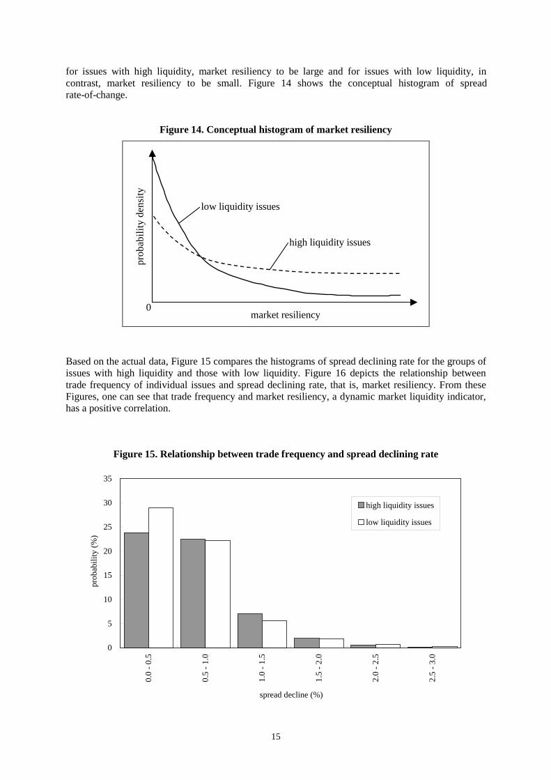
15

for issues with high liquidity, market resiliency to be large and for issues with low liquidity, incontrast, market resiliency to be small. Figure 14 shows the conceptual histogram of spreadrate-of-change.

Figure 14. Conceptual histogram of market resiliencypr

obab

ilit

y de

nsit

y

0market resiliency



Based on the actual data, Figure 15 compares the histograms of spread declining rate for the groups ofissues with high liquidity and those with low liquidity. Figure 16 depicts the relationship betweentrade frequency of individual issues and spread declining rate, that is, market resiliency. From theseFigures, one can see that trade frequency and market resiliency, a dynamic market liquidity indicator,has a positive correlation.

Figure 15. Relationship between trade frequency and spread declining rate

0

5

10

15

20

25

30

35

0.0

- 0.

5

0.5

- 1.

0

1.0

- 1.

5

1.5

- 2.

0

2.0

- 2.

5

2.5

- 3.

0

spread decline (%)

prob

abili

ty (

%)



16

Figure 16. Relationship between trade frequency and market resiliency

0.30

0.35

0.40

0.45

0.50

0.55

0.60

0.65

0.70

0.75

0.80

1 10 100 1000


aver

age

of n

egat

ive

mov

emen

t of

spre

ad (

%)

4. Event study: effects of tick size reduction on the TSE

The Tokyo Stock Exchange (TSE) changed the minimal price unit for trading (so-called “tick size”)on April 13 1998. The changes are listed in Table 2. As the right column of the table indicates, therewere three different changes depending on stock prices; those were 1/10, 1/5 and 1 (no change). Justas in Section 3, in this section we will try to analyse how these three changes may have affected themarket in terms of market liquidity, by using stocks from the TOPIX Electrical Machinery Index.

Table 2

Changes in tick size

Stock prices(X; yen)

Before change After change Scaled-down rate

000,1≤X 1 yen 1 yen 1

000,2000,1 ≤< X 10 yen 1 yen 1/10

000,3000,2 ≤< X 10 yen 5 yen 1/5

000,10000,3 ≤< X 10 yen 10 yen 1

000,30000,10 ≤< X 100 yen 10 yen 1/10

000,50000,30 ≤< X 100 yen 50 yen 1/5

000,100000,50 ≤< X 100 yen 100 yen 1

4.1 Data

For this analysis, we use data from the TOPIX Electrical Machinery Index (134 issues as of end-March 1998) downloaded from Bloomberg database. We analyse 55 trading days’ data, with a sampleperiod from March 10 1998 to May 29 1998. Of these 55 trading days, 23 trading days were dated

17

before April 13 and 32 trading days were after April 13. In Table 3, we categorised each issue inaccording to tick size reduced or unchanged. We analyse the data of 93 issues by subtracting thefollowing issues from the whole sample: those with an average trading time of less than ten times perday (26 issues), and those with trading prices which fluctuated over several different price rangesduring the sample period (from March 10 to May 29 1998) (15 issues).

Table 3

Grouping for analysis

Stock prices(X; yen)

Scaled-down rate Number of issues

000,2000,1 ≤< X 1/10 19

Tick-size-reduced issues 000,3000,2 ≤< X 1/5 2

000,30000,10 ≤< X 1/10 2

Tick-size-unchanged issues 000,1≤X 1 60

000,10000,3 ≤< X 1 10

(n.a.) 000,50000,30 ≤< X 1/5 0

000,100000,50 ≤< X 1 0

4.2 Effects on bid-ask spread

First, we analyse how changes in tick size affected a static market liquidity indicator, by examining thelevel of bid-ask spread. Theoretically, levels of bid-ask spread reflects both explicit trading costs suchas commissions and taxes, and implicit trading costs caused by a result of information asymmetryamong market participants. Besides these costs, however, there is a possibility that the tick size whichrelatively speaking had been regulated to be large, may have substantially influenced the level ofbid-ask spread in practice. For example, in looking at the bid-ask spread of the TSE stocks before thesize-change (Figure 17-1 and 17-2), there were some issues (with an actual market price over 1,000and less than 2,000 yen) with bid-ask spreads of mostly “10 yen” (Figure 17-1). In such cases, wecould consider the “largely regulated tick size (10 yen)” to have been the bid-ask spread’s minimumboundary, and as a result, all bid-ask spreads originally priced less than 10 yen had to be rounded up to10 yen. Therefore, when the tick size was set up to be larger than “the explicit plus implicit costs,”inappropriate trading costs may have existed for market participants. If these tick size changes mayhave removed the minimum boundary of trading costs, the average level of bid-ask spread should havedecreased significantly.

18

Figure 17-1. Histogram of bid-ask spreads (1):

A case where the tick size significantly affects the lower boundary of realised bid-ask spreads

0.00

0.10

0.20

0.30

0.40

0.50

0.60

0.70

0 10 20 30 40

bid-ask spread (yen)

prob

abil

ity

< Image >probability density of potentialbid-ask spread regardless oflimitation of tick size

< Image >proportions thatrealized bid-askspreads arerounded upbecause of theexistence ticksize

Figure 17-2. Histogram of bid-ask spreads (2):

A case where the tick size does not significantly affect the lower boundary of realised bid-ask spreads

0.00

0.10

0.20

0.30

0.40

0 10 20 30 40

bid-ask spread (yen)

prob

abili

ty

< Image >probability density of potentialbid-ask spread regardless oflimitation of tick size

< Image >proportions thatrealized bid-askspreads arerounded upbecause of theexistence ticksize

Figure 18 displays how changes in tick size might have affected the level of bid-ask spread, accordingto the categorisation in Table 3. While the tick-size-unchanged stocks show no apparent changes, thetick-size-reduced stocks show decreasing trends in those levels of bid-ask spreads. Next, we will testwhether the trends found in the tick-size reduced stocks are statistically significant.

Here, we consider the daily bid-ask spread (in logarithm) of each issue fluctuated stochasticallyaround its mean, and test whether the level of the mean may differ significantly between its before andafter scaled-down changes (April 13). We test t ratio by setting up the null hypothesis “there was nochange in the mean of bid-ask spread before and after April 13”, and the alternative hypothesis “themean of the bid-ask spread decreased after April 13.” Regarding the tick-size-unchanged stocks, only8 out of 70 issues (11%) rejected the null hypothesis at the 1% significant level. On the other hand, for

19

the tick-size-reduced stocks, 20 out of 23 issues (87%) rejected the null hypothesis. From these results,it is conceivable that a scale down in tick size significantly decreased the level of bid-ask spread.

Figure 18. Effects on the level of bid-ask spread

< tick-size-unchanged stocks >

0.0

0.5

1.0

1.5

2.0

before April 13 after April 13

not siginificantlydecrease( 62 stocks )

siginificantlydecrease( 8 stocks )

< tick-size-reduced stocks >

0.0

0.5

1.0

1.5

2.0


not significantlydecrease( 3 stocks )

significantlydecrease( 20 stocks )

Note: Vertical axes show how the level of bid-ask spread changed after the reduction of tick size, as a proportion ofthe level before the reduction of tick size, e.g. 1.5 denotes that the level of bid-ask spread increased by 50%.‘Significantly’ means that the null hypothesis “The reduction of tick size did not affect the level of bid-ask spread”is rejected at the 1% level of significance.

Regarding the above results, we can assume that tick size changes in the TSE on April 13 decreasedthe mean level of bid-ask spread, i.e. the average trading cost for market participants. This decrease intrading costs might have affected other indicators, by increasing market participants’ motivation totrade. Next, we test whether the tick size scale-down may also have influenced the trade frequency,dynamic market liquidity indicators and volatility of the trade execution price.

4.3 Effects on trade frequency

4.3.1 Effects on the number of quotes

If decreased trading cost results in increased motivation for market participants to trade, suchmechanism should first appear in the increasing number of revision in quotes.16 Figure 19 shows howchanges in tick size might have affected the number of quotes, according to the categorisation inTable 3. While in the tick-size-unchanged stocks no apparent changes can be found, thetick-size-reduced stocks show an increasing trend in the number of quotes. In order to test whetherthese trends are statistically significant, here we again test t ratio by setting up the null hypothesis“there was no change in the number of quotes from before April 13 to after April 13”, and thealternative hypothesis “there was an increase in the number of quotes after April 13.” Regarding thetick-size-unchanged stocks, only 1 out of 70 issues (1%) rejected the null hypothesis at the 1%significant level. On the other hand, for the tick-size-reduced stocks, 19 out of 23 issues (83%)rejected the null hypothesis. From these results, it is conceivable that the tick size scale-down hadsignificantly increased the number of revisions in quotes.

16Because of the limited data available, “the number of quotes” will be used here as a proxy of “the number of tradeorders.”

20

Figure 19. Effects on the number of quotes


0.0

0.5

1.0

1.5

2.0

2.5

3.0


significantlyincrease( 19 stocks )

not significantlyincrease( 4 stocks )


0.0

0.5

1.0

1.5

2.0

2.5

3.0


significantlyincrease( 1 stock )


Note: Vertical axes show how the number of quotes changed after the reduction of tick size, as a proportion of thenumber before the reduction of tick size, e.g. 1.5 denotes that the number of quotes increased by 50%.‘Significantly’ means that the null hypothesis “The reduction of tick size did not affect the number of quotes” isrejected at the 1% level of significance.

4.3.2 Effects on the number of trades

Here again, we see how changes in tick size might have affected the trade execution frequency inFigure 20. Although Figure 20 shows similarity to Figure 19, the significance of the t ratio testdecreased more or less.

Figure 20. Effects on the number of trades


0.0

0.5

1.0

1.5

2.0





0.0

0.5

1.0

1.5

2.0




Note: Vertical axes show how the number of trades changed after the reduction of tick size, as a proportion of thenumber before the reduction of tick size, e.g. 1.5 denotes that the number of trades increased by 50%.‘Significantly’ means that the null hypothesis “The reduction of tick size did not affect the number of trades” isrejected at the 1% level of significance.

4.4 Effects on the dynamic market liquidity indicators

4.4.1 Effects on volatility of bid-ask spreads

Because of the reduction in tick size, more precise pricing in limit orders became available for marketparticipants. As a result, we can expect that bid-ask spread’s fluctuation might have become moredynamic, reflecting implicit trading costs more precisely. In this section, we see the volatility

21

calculated from every five minutes’ bid-ask spreads, regarding the influence of tick size changes ondynamics of the bid-ask spread.

Figure 21 shows how changes in tick size might have affected the intraday volatility of bid-askspreads. The tick-size-reduced stocks show an increasing trend in the volatility of bid-ask spreads.Here, we test t ratio by setting up the null hypothesis “there was no change in the volatility of bid-askspread from before April 13 to after April 13,” and the alternative hypothesis “there was an increase inthe volatility of bid-ask spread after April 13.” Regarding the tick-size-unchanged stocks, only 1 out of70 issues (1%) rejected the null hypothesis at the 1% significant level. On the other hand, for thetick-size-reduced stocks, 22 out of 23 issues (96%) rejected the null hypothesis. From these results, itcan be said that the reduction in tick size had eased the degree of freedom in bid-ask spreadfluctuation. And, we could conceive that the spread’s fluctuation had become more sensitive to reflectchanges in implicit costs caused by information asymmetry.

Figure 21. Effects on volatility of bid-ask spreads


0.0

0.5

1.0

1.5

2.0



0.0

0.5

1.0

1.5

2.0



not significantlyincrease( 1 stock )



Note: Vertical axes show how the volatility of bid-ask spreads changed after the reduction of tick size, as aproportion of the level before the reduction of tick size, e.g. 1.5 denotes that the volatility of bid-ask spreadsincreased by 50%. ‘Significantly’ means that the null hypothesis “The reduction of tick size did not affect thevolatility of bid-ask spreads” is rejected at the 1% level of significance.

4.4.2 Effects on market impact

Figure 22 shows the effects of the tick size reduction on market impact, which is one of the twodynamic indicators of market liquidity. Some of the tick-size-unchanged stocks show an increasingtrend in market impact compare to the tick-size reduced stocks. We test t ratio by setting up the nullhypothesis “there was no change in market impact from before April 13 to after April 13,” and thealternative hypothesis “there was an decrease in market impact after April 13.” The results show thatthe two groups are not significantly different. From these results, it can be said that the reduction intick size did not affect averaged market impact.

22

Figure 22. Effects on market impact

0.0

0.5

1.0

1.5

2.0


not siginificantlydecrease( 62 stocks )



0.0

0.5

1.0

1.5

2.0




< tick-size-unchanged stocks

Note: Vertical axes show how the level of market impact changed after the reduction of tick size, as a proportion ofthe level before the reduction of tick size, e.g. 1.5 denotes that market impact increased by 50%. ‘Significantly’means that the null hypothesis “The reduction of tick size did not affect the level of market impact” is rejected atthe 1% level of significance.

4.4.3 Effects on market resiliency

Figure 23 shows the effects of the tick size reduction on market resiliency, another dynamic indicatorof market liquidity. The tick-size-reduced stocks show an increasing trend in the convergence speed ofbid-ask spreads, that is, market resiliency tends to increase by the reduction. Here, we test t ratio bysetting up the null hypothesis “there was no change in market resiliency from before April 13 to afterApril 13,” and the alternative hypothesis “there was an increase in market resiliency after April 13.”Regarding the tick-size-unchanged stocks, only 1 out of 70 issues (1%) rejected the null hypothesis atthe 1% significant level. On the other hand, for the tick-size-reduced stocks, 10 out of 23 issues (43%)rejected the null hypothesis. These results imply that the reduction in tick size motivated traders tosubmit limit orders more frequently and, as a result, increased market resiliency.

Figure 23. Effects on market resiliency

0.5

1.0

1.5

2.0


siginificantlyincrease( 1 stock )

not siginificantlyincrease( 69 stocks )


0.5

1.0

1.5

2.0





Note: Vertical axes show how the level of market resiliency changed after the reduction of tick size, as a proportionof the level before the reduction of tick size, e.g. 1.5 denotes that market resiliency increased by 50%.‘Significantly’ means that the null hypothesis “The reduction of tick size did not affect the level of marketresiliency” is rejected at the 1% level of significance.

4.5 Effects on price volatility

Finally, we analyse how changes in tick size might have affected the volatility in market prices. Thereduction in tick size would induce more precise prices in ordering and provide more detailed priceinformation for market participants at the same time. Therefore, we may assume that the reduction in

23

tick size might have improved market efficiency (i.e. an increase in the amount of information whichreflects on prices) and therefore decreased the volatility of market prices. Next, by using tradeexecution price as market price, we test whether size changes in tick size significantly decreasedvolatility of market prices as calculated every five minutes.

Figure 24 compares the daily averages of intraday volatility of trade prices before and after the changein tick size on April 13. In the t ratio test, we consider the null hypothesis “there were no changes inthe daily average of intraday trade price volatility from before April 13 to after April 13,” and thealternative hypothesis “the intraday price volatility had decreased after April 13.” Regarding thetick-size-unchanged stocks, only 9 out of 70 issues (13%) rejected the null hypothesis at the 1%significant level. On the other hand, for the tick-size-reduced stocks, 17 out of 23 issues (74%)rejected the null hypothesis. From these results, we could assume that the reduction in tick size hadimproved market efficiency.

Figure 24. Effects on price volatility

0.994

0.996

0.998

1.000

1.002

1.004


not siginificantlydecrease( 60 stock )



0.994

0.996

0.998

1.000

1.002

1.004





Note: Vertical axes show how the level of intraday price volatility changed after the reduction of tick size, as aproportion of the level before the reduction of tick size, e.g. 1.5 denotes that intraday price volatility increased by50%. ‘Significantly’ means that the null hypothesis “The reduction of tick size did not affect the intraday pricevolatility” is rejected at the 1% level of significance.

5. Summary and future work

This paper introduces both the definition of market liquidity and the methods of measuring marketliquidity indicators proposed by Muranaga and Shimizu (1999), and, within this framework, analysesmarket liquidity of the individual stocks listed on the TSE. This paper is unique in that it utilisestick-by-tick data of the TSE in order to analyse dynamics of market liquidity. By conducting anempirical analysis based on the TSE tick-by-tick data, we have obtained results that if the monitoringfrequency does not increase directly in accordance with the change in trade frequency, there is apossibility that the changes in market conditions may have been overlooked. Also there are positivecorrelations between trade frequency and each of the three indicators of market liquidity. Through theevent study on the effects of the reduction in tick size of the TSE on April 13 1998, we have shown apossibility that the reduction in tick size might have reduced implicit trading costs and improved pricediscovery function in the TSE. Therefore, we can point out that (1) it is deemed necessary to take intoaccount the effects of data monitoring frequency in analysing market dynamics, (2) trade frequency ispositively correlated with market liquidity, and (3) the change in tick size could affect trading costsand market liquidity and efficiency.

In conducting empirical analysis, we first monitored intraday fluctuation patterns of trade volume,bid-ask spread, and price volatility of issues listed on the first session of the TSE. We observed thattrade volume and bid-ask spread for a W-shape, and that trade volume, bid-ask spread, and pricevolatility all show an substantial increase towards the closing of the afternoon session. In addition, inanalysing the relationship between trade frequency and market liquidity, we focused on a static market

24

liquidity indicator (bid-ask spread) and dynamic indicators (market impact and market resiliency). Wehave considered how to estimate market resiliency in the absence of volume data such as trade orderflows or order book profile, and found that declining rate of bid-ask spread can, with certain extent ofexplanatory power, be a proxy of market resiliency.

In order to avoid the problem of quote disappearance unique to the TSE at which exchange-designatedliquidity providers do not exist, we have dealt only with issues with relatively high liquidity. However,disappearance of bid or ask signifies evaporation of market liquidity because it reveals the fact thatmarket orders (sell/buy), which need to be traded immediately, will not be executed. Suchphenomenon is indeed one of the most important issues to be explored when discussing marketliquidity of the TSE. It will be our future work to explore and gain insights about this issue based onour results which were obtained by analysing issues with relatively high market liquidity. Sincemarket liquidity is a total market depth which includes effective supply and demand, it changesdynamically according as the trading incentives of market participants change. In order to observe thiskind of development, the further refinement of dynamic indicators, especially market resiliency will benecessary. Specifically, how to express market resiliency in cases where new market orders areexecuted continuously and the bid-ask spread fails to resume its stationary state.

Because of limitations on data availability, past studies mainly tried to extract information contents ofthe market by analysing market price changes along with time horizon. These studies were based onthe assumption that all information, including trade volume, is reflected in market prices. However,market microstructure theory argues that information about order flows and trade volume not reflectedin market prices is profitable for market participants, and that games based on such information affectmarket behaviour. In other words, when one wishes to analyse the market at a micro level, factors suchas the budget constraints of individual market participants, restrictions on short-selling, and loss-cutrules may not be neglected. By making more use of information about the volume of order flows andtrade executions, which has recently become increasingly available, market analysis in the future willbe required to be conducted in three dimensions: time, price, and volume. If we can monitortick-by-tick dynamics of the market liquidity by using more sophisticated indicators, we may be ableto gain more insights about some critical issues such as the mechanism of market liquidityevaporation.

25

References

Engle, R F and J Lange, 1997, “Measuring, Forecasting and Explaining Time Varying Liquidity in theStock Market,” NBER Working Paper No. 6129.

Fletcher, 1995, “The Role of Information and the Time between Trades: An Empirical Investigation,”Journal of Financial Research, Vol. 18, No.2.

Hausman, J A, A W Lo and A C MacKinlay, 1992, “An Ordered Probit Analysis of Transaction StockPrices,” Journal of Financial Economics, Vol. 31, No.3.

Kyle, A S, 1985, “Continuous Auctions and Insider Trading,” Econometrica, Vol. 53, No. 6.

Lehman, B N and D M Modest, 1994, “Trading and Liquidity on the Tokyo Stock Exchange: A Bird’sEye View,” Journal of Finance (July 1994).

Lehman, B N, D M Modest, M Azuma and H Koizumi, 1994, “Liquidity and Market Microstructureon the Tokyo Stock Exchange (in Japanese),” Toushikougaku (Spring 1994).

Lindsey, R R and U Schaede, 1992, “Specialist vs. Saitori: Market-Making in New York and Tokyo,”Financial Analysis Journal (July-August 1992).

Muranaga, J and M Ohsawa, 1997, “Measurement of Liquidity Risk in the Context of Market RiskCalculation,” The Measurement of Aggregate Market Risk, Bank for International Settlements.

Muranaga, J and T Shimizu, 1999, “Market Microstructure and Market Liquidity,” mimeo.

O’Hara, M, 1995, Market Microstructure Theory, Blackwell Publishers Inc.

Ohtsuka, A, 1995, “An Analysis of Intraday Stock Price Movement Focusing on Trade Imbalance (inJapanese),” Toushikougaku (Autumn 1995).

cgfs publications - dynamics of market liquidity of ... · dynamics of market liquidity of japanese...

Documents