ch 7.5: homogeneous linear systems with constant coefficients we consider here a homogeneous system...
Post on 21-Dec-2015
223 views
TRANSCRIPT

Ch 7.5: Homogeneous Linear Systems with Constant Coefficients
We consider here a homogeneous system of n first order linear equations with constant, real coefficients:
This system can be written as x' = Ax, where
nnnnnn
nn
nn
xaxaxax
xaxaxax
xaxaxax
2211
22221212
12121111
nnnn
n
n
m aaa
aaa
aaa
tx
tx
tx
t
21
22221
11211
2
1
,
)(
)(
)(
)( Ax

Solving Homogeneous System
To construct a general solution to x' = Ax, assume a solution of the form x = ert, where the exponent r and the constant vector are to be determined.
Substituting x = ert into x' = Ax, we obtain
Thus to solve the homogeneous system of differential equations x' = Ax, we must find the eigenvalues and eigenvectors of A.
Therefore x = ert is a solution of x' = Ax provided that r is an eigenvalue and is an eigenvector of the coefficient matrix A.
0ξIAAξξAξξ rreer rtrt
Example 1: Direction Field (1 of 9)
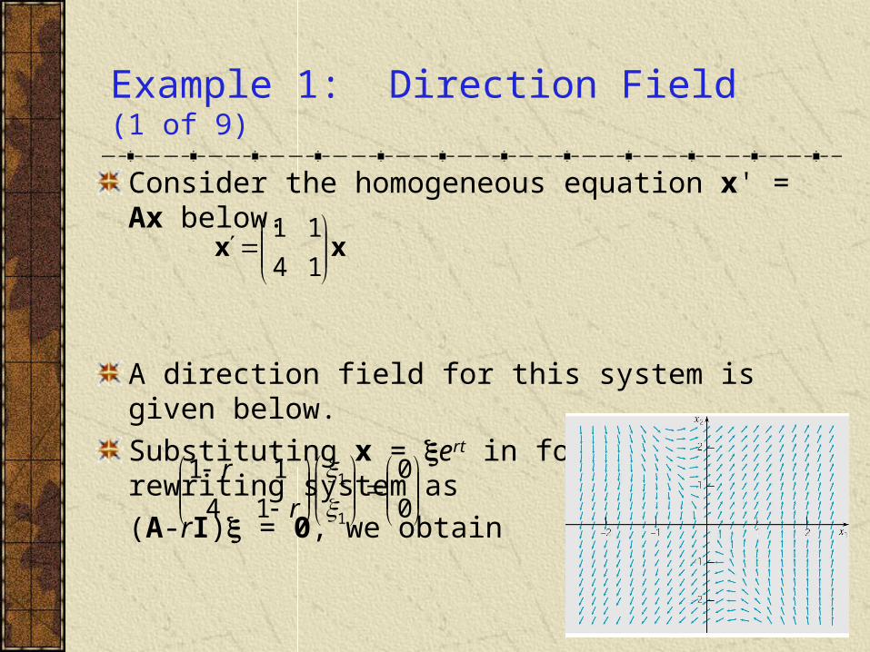
Consider the homogeneous equation x' = Ax below.
A direction field for this system is given below.
Substituting x = ert in for x, and rewriting system as
(A-rI) = 0, we obtain
xx
14
11
0
0
14
11
1
1
r
r

Example 1: Eigenvalues (2 of 9)
Our solution has the form x = ert, where r and are found by solving
Recalling that this is an eigenvalue problem, we determine r by solving det(A-rI) = 0:
Thus r1 = 3 and r2 = -1.
0
0
14
11
1
1
r
r
)1)(3(324)1(14
11 22
rrrrr
r
r

Example 1: First Eigenvector (3 of 9)
Eigenvector for r1 = 3: Solve
by row reducing the augmented matrix:
0
0
24
12
0
0
314
131
2
1
2
1
0ξIA r
2
1choosearbitrary,
1
2/12/1
00
02/11
000
02/11
024
02/11
024
012
)1(
2
2)1(
2
21
ξξ cc
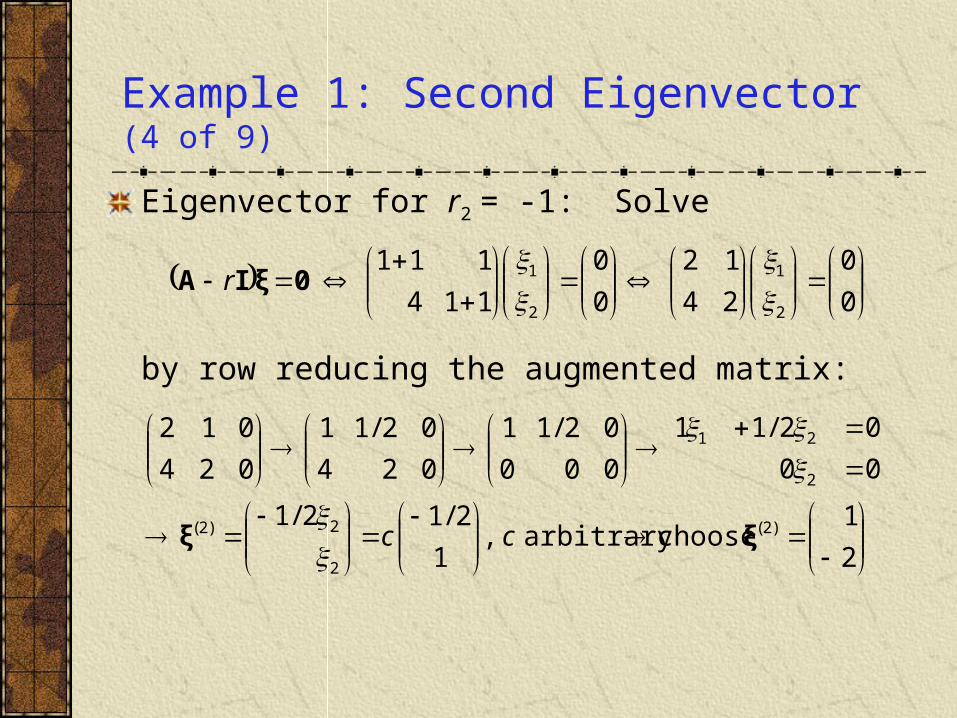
Example 1: Second Eigenvector (4 of 9)
Eigenvector for r2 = -1: Solve
by row reducing the augmented matrix:
0
0
24
12
0
0
114
111
2
1
2
1
0ξIA r
2
1choosearbitrary,
1
2/12/1
00
02/11
000
02/11
024
02/11
024
012
)2(
2
2)2(
2
21
ξξ cc

Example 1: General Solution (5 of 9)
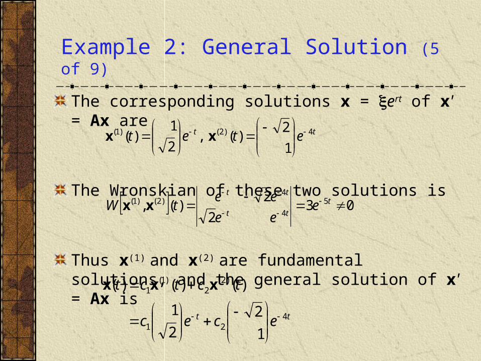
The corresponding solutions x = ert of x' = Ax are
The Wronskian of these two solutions is
Thus x(1) and x(2) are fundamental solutions, and the general solution of x' = Ax is
tt etet
2
1)(,
2
1)( )2(3)1( xx
0422
)(, 2
3
3)2()1(
t
tt
tt
eee
eetW xx
tt ecec
tctct
2
1
2
1
)()()(
23
1
)2(2
)1(1 xxx
Example 2: (1 of 9)
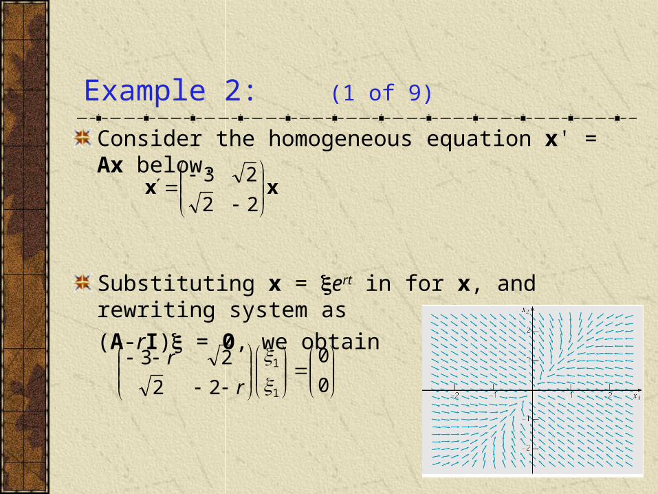
Consider the homogeneous equation x' = Ax below.
Substituting x = ert in for x, and rewriting system as
(A-rI) = 0, we obtain
xx
22
23
0
0
22
23
1
1
r
r

Example 2: Eigenvalues (2 of 9)
Our solution has the form x = ert, where r and are found by solving
Recalling that this is an eigenvalue problem, we determine r by solving det(A-rI) = 0:
Thus r1 = -1 and r2 = -4.
)4)(1(452)2)(3(22
23 2
rrrrrr
r
r
0
0
22
23
1
1
r
r

Example 2: First Eigenvector (3 of 9)
Eigenvector for r1 = -1: Solve
by row reducing the augmented matrix:
0
0
12
22
0
0
122
213
2
1
2
1
0ξIA r
2
1choose
2/2
000
02/21
012
02/21
012
022
)1(
2
2)1( ξξ
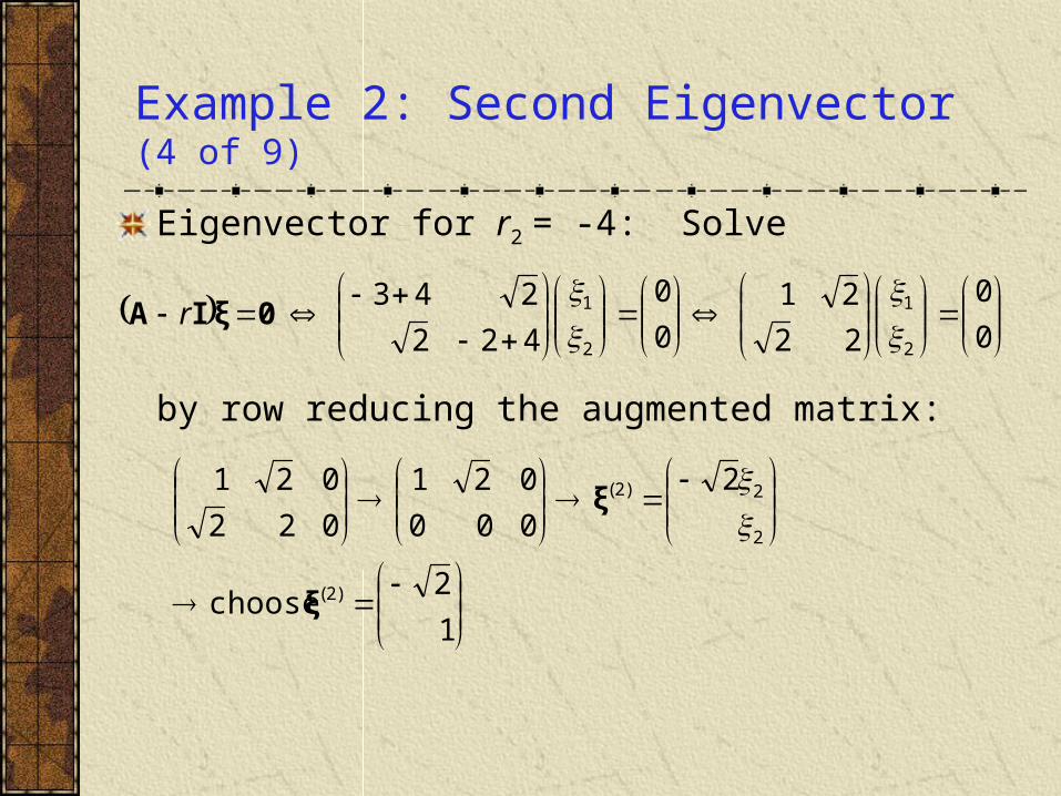
Example 2: Second Eigenvector (4 of 9)
Eigenvector for r2 = -4: Solve
by row reducing the augmented matrix:
0
0
22
21
0
0
422
243
2
1
2
1
0ξIA r
1
2choose
2
000
021
022
021
)2(
2
2)2(
ξ
ξ
Example 2: General Solution (5 of 9)
The corresponding solutions x = ert of x' = Ax are
The Wronskian of these two solutions is
Thus x(1) and x(2) are fundamental solutions, and the general solution of x' = Ax is
tt etet 4)2()1(
1
2)(,
2
1)(
xx
032
2)(, 5
4
4)2()1(
t
tt
tt
eee
eetW xx
tt ecec
tctct
421
)2(2
)1(1
1
2
2
1
)()()(
xxx

Eigenvalues, Eigenvectors and Fundamental Solutions
In general, for an n x n real linear system x' = Ax:All eigenvalues are real and different from each other.
Some eigenvalues occur in complex conjugate pairs.
Some eigenvalues are repeated.
If eigenvalues r1,…, rn are real & different, then there are n corresponding linearly independent eigenvectors (1),…, (n). The associated solutions of x' = Ax are
Using Wronskian, it can be shown that these solutions are linearly independent, and hence form a fundamental set of solutions. Thus general solution is
trnntr netet )()()1()1( )(,,)( 1 ξxξx
trnn
tr necec )()1(1
1 ξξx

Hermitian Case: Eigenvalues, Eigenvectors & Fundamental Solutions
If A is an n x n Hermitian matrix (real and symmetric), then all eigenvalues r1,…, rn are real, although some may repeat.
In any case, there are n corresponding linearly independent and orthogonal eigenvectors (1),…, (n). The associated solutions of x' = Ax are
and form a fundamental set of solutions.
trnntr netet )()()1()1( )(,,)( 1 ξxξx
Example 3: Hermitian Matrix (1 of 3)
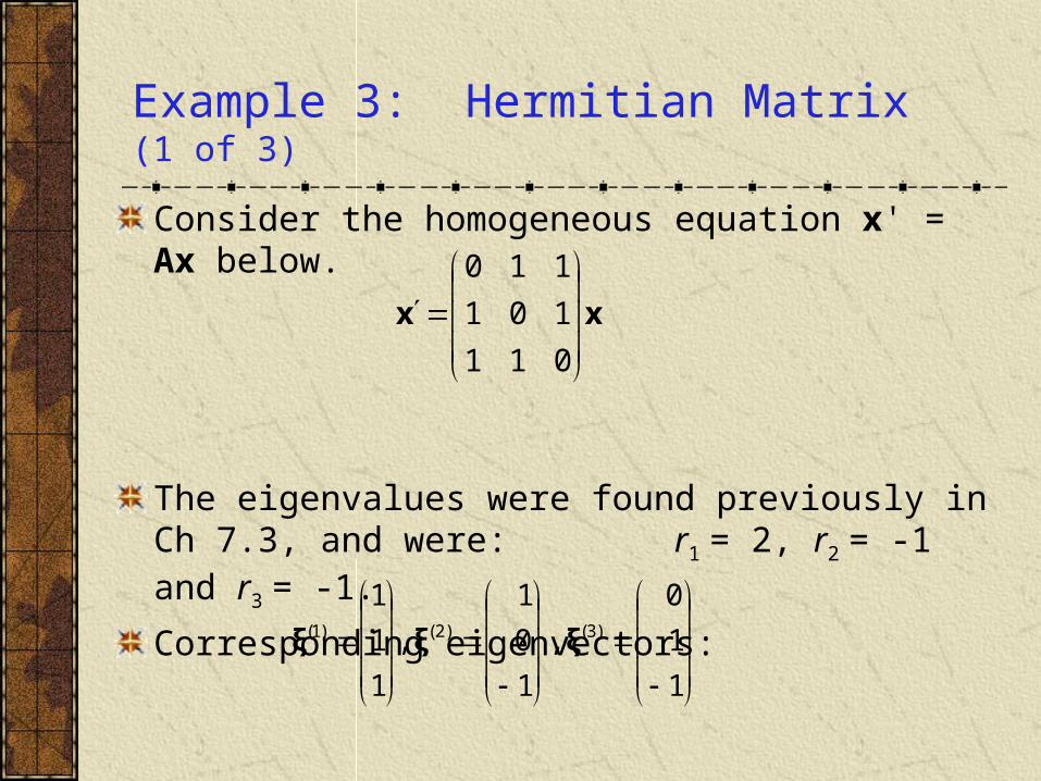
Consider the homogeneous equation x' = Ax below.
The eigenvalues were found previously in Ch 7.3, and were: r1 = 2, r2 = -1 and r3 = -1.
Corresponding eigenvectors:
xx
011
101
110
1
1
0
,
1
0
1
,
1
1
1)3()2()1( ξξξ

Example 3: General Solution (2 of 3)
The fundamental solutions are
with general solution
ttt eee
1
1
0
,
1
0
1
,
1
1
1)3()2(2)1( xxx
ttt ececec
1
1
0
1
0
1
1
1
1
322
1x