Ch ges In the Ecosystem ofRivers Inlet, British Columbia:

19501 Y& the Pre·ent

Fisheries Centre, Univenity of British Columbia, Canada

Changes in the Ecosystemof Rivers Inlet, British Columbia:

1950 YB. the Present

8eDattlDthelJaJitlSuzukiFoundaiiaJ

by

Stephen Watkinsonand

Daniel Pauly

The Fisheries Centre, University ofBritish Columbia

2204 Main MallVancouver, B. C., Canada

1999

Abstract

Rivers Inlet, a fjord-like area of 1000 km2 on the central coast of British Columbia, Canada, isbriefly described, as are the fisheries for salmon (five Oncorhynchus species) and for speciesother than salmon, notably halibut and rockfishes.

It is shown that both the salmon catches and the fishing effort directed at salmon declined from1950 to the present. Commercial catches, throughout the period were about ten times larger thaneither the recreational or Aboriginal fisheries, though this is based, for the two smaller fisheries,on very preliminary estimates of catch.

Non-salmon catches are also declining, due to an exponential increase in fishing effort, leading tolow catch per unit of effort. The species exploited by the fishery are in general long-lived, andthus highly vulnerable to overfishing. The data suggest much reduced stock biomasses for thesespeCIes.

Ecosystem models representing two states of the Rivers Inlet ecosystems (early 1950s, and early1990s) were constructed. These models suggest that the mean trophic level of the catch landed bythe fisheries in the Rivers Inlet area has declined from the 1950s to the present, in line with theglobal trend of 'fishing down marine food webs'.

Effort reductions, structured around an ecosystem rebuilding strategy, are required to reversethese trends. Such efforts would also require a much better database than presently available onthe fisheries of Rivers Inlet.

TABLE OF CONTENTS

ABSTRACT 1

TABLE OF CONTENTS 11

LIST OF FIGURES 11

LIST OF TA,BLES 11

INTRODUCTION 1THE ECOSYSTEM OF RIvERS INLET 1FISHERY CATCH AND EFFORT ANALYSIS 2SALMON CATCH AND EFFORT 2

Commercial sector 2Sports sector 3Aboriginal sector 3

NON-SALMON CATCH AND EFFORT 4CONCLUS~ON FROM COMPARISONS OF ECOSYSTEM (ECOPATH) MODELS .4OVERALL CONCLUSIONS 5REFERENCES 5

APPENDIX 1. METHODOLOGICAL NOTES FOR THE CATCH AND EFFORT ANALYSES 9

COMMER<):IAL EFFORT ANALySIS 9SPORTS CATCH AND EFFORT ANALYSIS 9ABORIGINt..L CATCH AND EFFORT ANALYSIS 10

BASIC FEATURES OF THE ECOPATH MODEL 10MEASURING THE MODEL SURFACE AREA FOR RIvERS INLET 11CONSTRUCTING THE MODELS 11

1991-1995 Model 111951-1955 Model 13

BALANCING THE MODELS· 141991-1995 Model 141951-1955 Model 16

APPENDIX 4. ECOPATH MODEL INPUTS AND ESTIMATES 18

APPENDIX 5. ECOPATH MODEL OUTPUTS 19

APPENDIX 6. TROPIDC FLOW DIAGRAM 20

LIST OF FIGURES

Figure 1. Map of the model boundaries 1Figure 2. Catch and effort levels for the commercial salmon fleet for 1964-1993 2Figure 3. Catch per unit effort for the commercial salmon fleet 1964-1993 3Figure 4. Catch and effort levels for the non-salmon commercial fleet for 1964-1993 .4Figure 5. Catch per unit effort for the non-salmon commercial fleet for 1964-1993 .4Figure 6 Flowchart of the 1990s Ecopath model... 20

LIST OF TABLES

Table 1. Biomass changes to convert the 1990s model to a 1950s model of the same ecosystem 14Table 2. Diet composition for groups used in Ecopath models 17Table 3. Basic input parameters for both Rivers Inlet models 18Table 4. Output statistics for both Rivers Inlet models 19

ii

hand, to track changes in the River Inletsecosystem that may be due to changes inland use patterns. For this reason, and due toan overall scarcity of readily availablestatistical information on the fisheries , thisreport can only present tentative, andpreliminary conclusions.

To interpret the fisheries data, twoecosystem models were constructedfocusing on the Rivers Inlet region. The firstof these covers the time period 1951-1955,while the second the time period from 1991­1995.

THE ECOSYSTEM OF RIVERS INLET

The Rivers Inlet region, of about 1000 km2,

located on the central coast of BritishColumbia approximately 400 kilometersnorthwest from Vancouver, is the focal areaof this study (Fig. 1). The Inlet is a coastalfjord characterized by steep walls withdepths reaching as much as 325 meters. The

Wannock River feedsthe Inlet, which is themain outlet forOwikeeno Lake.

The boundaries ofthis ecosystem, asdefmed here, followthose used by theDepartment ofFisheries and Oceans(DFO) to defmeStatistical Area 9. In985, however, DFOchanged theseboundaries, i.e.,eliminated thesegment thatextended west ofCalvert Island.Therefore, theecosystem used forthe model of 1991­1995 was defined bythe boundaries forStatistical Areas 9and 109. This kept

IA>: ! _..:~ ~ ..:,.,

L...-----r;.::;;::::::;:------r--.....

Figure 1. Map showing the boundaries for DFO statistical areas 9 and109, used as the boundaries for the Ecopath models. The zone outlined·in red (solid) depicts area 9, while the zone outlined in green (dotted)represents area 109. These two zones were the boundaries for the 1990smodel. The red section combined with the dark blue (dashed) sectionrepresents area 9 as it was up until 1985, and was used as the boundaryfor the 1950s model.

INTRODUCTION

Rivers Inlet is a large fjord along the centralcoast of British Columbia (Fig. 1), importantfor commercial, recreational, and Aboriginalfishers. The fish species that are exploitedinclude five salmon species, and eulachon,halibut, and rockfish. At one time, theRivers Inlet sockeye fishery was the secondlargest in British Columbia, right after theFraser River fishery. The first commercialsalmon fleet and canning plant appeared inRivers Inlet in 1882 (Wood 1970).

The Rivers Inlet ecosystem has experiencedmany changes since, and especially in thelast 50 years, some as a result of logging theadjacent watersheds, some as results offishing, and others due to a mixture ofcauses. This report documents some of thesechanges, and attempts to identify changesthat may have been due to changes in fishingpatterns. No attempt is made, on the other

1

Figure 2. Catch and effort levels for the commercial salmonfleet for 1964-1993. The effort declines constantly with thecatch declining overall as well but with some fluctuations.

5.0 £"'=...4.0 ~

~3.0 ~"CI

2.0 ..§''-'....

1.0 ~:::::

0.0 r-"l

1992

Year

declined over the years, along with fishingeffort. This resulted in a catch per unit effort(CPUE) that oscillates, but without majordeclining or increasing tend (Fig. 3).

The catch can be seen to drop off around1980, as the seine fleet was removed fromthe fishing fleet in the Rivers Inlet region.Due to various regulations, effort hasdecreased steadily from around 1980 to thepresent, with no commercial salmon fishingin the past few years. One exception to thisgeneral trend is Chinook, whose localpopulation has been the object of muchenhancement activity (Larkin and Slaney1997). Concerning Rivers Inlet salmon, itshould be noted that if fishing effort had notdeclined, the results could have beendisastrous. Indeed, though our measure ofnominal effort has declined, effective effortremained relatively high, due to

Fuel supply is a major cost factor in fishing,which the catch must offset.

SALMON CATCH AND EFFORT

Commercial sector

Total salmon catch and total effort werecalculated for the period 1960-1993, thenboth time series were smoothed by using arunning average over 5 years, such as tohighlight key features of the series (Fig. 2).

As might be seen, salmon catches have

1968 1972 1976 1980 1984 1988

1.61.4

~ 1.2... 1.0

~ 0.8.cl 0.6~U 0.4

0.20.0 '--_--L.-_-'---_.....I..-_-..L_----l.L------JL-_J...J

1964

Catch data was divided into twocategories, 'salmon' and 'non­salmon', for which catches weresummed after conversion tometric units (tonnes). The salmoncategory is made up the fivesalmon species (pink.,Oncorhynchus gorbuscha; Chum,0. keta; Coho, 0. kisutch;Sockeye, 0. nerka; and Chinook,0. tshawytscha) , while the non-salmon category comprised of all otherspecies reported in the catch statistics. Theexceptions to this were herring (Clupeaharengus pallasi), for which catch data wereavailable, but without corresponding effortdata, and abalone and clams, which areharvested by diving.

Total fleet horsepower . fishing days('horsepower days') was selected asmeasure of aggregated fishing effort.Beverton and Holt (1957) showed that, forNorth Sea trawlers, there is a directrelationship between fishing power andengine power; Dalzell et al. (1987) showedthis to apply as well, in the Philippines, to awide range of fishing craft. Anotheradvantage of horsepower days asmeasurement for effort is that they relate tofuel consumption (Levi and Grannetti 1973).

FISHERY CATCH AND EFFORT ANALYSIS

Rivers Inlet is an important fishing area forthe three major fisheries user groups inBritish Columbia: commercial, recreationaland Aboriginal. Each sector was examinedin terms of its impact on theecosystem. The assessmentsconsisted of compiling the catchtrends over the years where datais available, as well as the fishingeffort expended to produce thosecatches.

the commercial catch statistics and the sizeof the modeled area reasonably consistent,especially as the difference occurs in theopen ocean section of the ecosystem, whereconditions are more homogeneous thaninshore.

2

0.80>; 0.70~ 0.60c!- 0.50~

~ 0040;; 0.30~ 0.20o 0.10

0.00 '"

1964 1968 1972 1976 1980 1984 1988 1992

Year

fishers are now using more powerfulengines than in the past. One importantitem to note is that the highestestimated sport catch is about 10 timeslower than the lowest commercial catch(compare to FigA).

Aboriginal sector

The land surrounding Rivers Inletincludes the traditional territory of theOweekeno First Nation. No catch andeffort statistics could be found for thisuser group; however, a rough estimateof catches is required for an analysis ofthe fisheries of the region to becomplete.

Figure 3. Catch per unit effort for the commercialsalmon fleet, 1964-1993. Although CPUE didfluctuate, the overall trend follows a straight linedepicted as the mean.

technological advances such as echosounders and nylon gillnets. Thus, by 1955,approximately 80 percent of the salmon fleetwas using nylon nets instead of the cotton orlinen made nets that were in exclusive useearlier (Wood 1970).

Sports sector

Rivers Inlet is a major fishing destination forrecreational fishers, hosted at about 20fishing lodges, of both the permanent andfloating (transient) types. Continuous timeseries of sports fishing catch and effort datacould not be found; indeed, the only suitabledata found pertained to salmon species, forthe early 1950s and late 1990s. Intermediatevalues were interpolated for the missingyears, as described in Appendix 1. [Notethat given the relatively small catch of therecreational fishery relative to thecommercial fishery, our having to useinterpolated data had very little effect on thecomparison between fisheries; see below].

Even though the catch for the sports fisheryhas increased over the years, their CPUE hasremained stable at 0.08 kg per horsepowerday, due to increased effort. The increase ineffort is in part due to the fact that the

Here, catch estimates were obtained byworking from salmon consumptionrates estimated for First Nations peopleduring pre-contact times. Hewes (1973)does not give an estimate for theOweekeno First Nation but estimates

that other First Nations nearby (Nuxalk;Heiltsuk) consumed "about 500 pounds" perperson per year.

Using such a figure, it must be stressed, willlead to overestimates of catch: it can safelybe assumed that the members of FirstNations today do not eat the same amount ofsalmon as their ancestors did, given thepresent availability of other sources ofanimal protein. Another reason is that thecatch estimate is based on people registeredwith the Oweekeno First Nation, of whichmany reside off reserve. Further, eventhough many off-reserve people return toRivers Inlet during the fishing season, not alldo. Finally, the population estimates alsoinclude children, who can safely be assumedto consume far less than 500 Ibs. of salmonper year. The Aboriginal catch estimates ofabout 35 tonnes per year is thus an extremeoverestimate, to be used only for order-of­magnitude comparisons with the commercialand recreational sectors. It should be notedthat this estimate, while slightly higher thanthat of the recreational fishery, is still in theorder of one tenth the commercial fishery.

3

Figure 4. The catch and effort levels for the non-salmoncommercial fleet for 1964-1993. Note the rise in effortfrom 1988-1994 and the corresponding drop in catch inthe early 1990s.

250~....200 ~

150 ~100~50 e-O ]....

~

Year

The most notable that occurred between the1950s and the present is that the commercialfishery earlier relied on fish with a meantrophic level of 3.83, while it now relies onfish (including invertebrates) with a tropiclevel of to 3.67. As trophic levels indicatethe position of an organism with the foodweb of a given ecosystem, this resultindicates that the commercial fleet has been'fishing down the food web' as described inPauly et ai. (1998) for fisheries throughoutthe world. Fishing down the food webimplies a transition from catches consistingprimarily of long-lived, fish-eating fish tocatches consisting of short-lived, small,

4.0re 3.0~:; 2.0

Col

~ 1.0u

0.01964 1%8 1972 1976 1980 1984 1988 1992

and

Unfortunately, data were not available thatwould have enabled estimation of therecreational and Aboriginal components ofthe non-salmon catch and effort.

Aboriginal effort data could not befound. In order to obtain anapproximate measure of Aboriginalfishing effort, we assumed that theAboriginal fishers are as efficient asthe commercial fishers. Thus, theestimated Aboriginal catch wasdivided into the CPUE (i.e.,catch/effort) of the commercialfishery. This resulted in a CPUE ofabout 0.173 kg per horsepower day.

NON-SALMON CATCH AND EFFORT

The non-salmon catch and effortanalysis included all the speciesreported in the DFO catch statisticssummaries except for abalone, clams,and herring, which did not havecomplete time series for both catcheffort.

The catch and effort data for the non-salmonfishery as defmed here remained fairlyconstant in the 1960s and early 1970s. Afterthis, effort increased dramatically, while thecatch started to decline (Fig. 4). This resultsin CPUE dropping to a very low level in the1980s and 1990s, indicating much reducedabundances on the ground (Fig. 5). Fishershave to work harder in order to catch less.

CONCLUSION FROMCOMPARISONS OF ECOSYSTEM(ECOPATH) MODELS

The major aim of constructingecosystems representing the pastand present states of the RiversInlet ecosystems was to check ifthe observed changes in variousgroups (see above) could beaccommodated in terms of thefluxes of fluxes of matter (fishfood, catches) that are implied.Appendices 2-6 document thesteps taken to construct andbalance the models in questions.

0.12

~ 0.1"Cl

~ 0.08.l:l

~ 0.06~-~ 0.04;:Jl:lo;U 0.02

o1964 1968 1972 1976 1980 1984 1988 1992

Year

Figure 5. Catch per unit effort for the non-salmoncommercial fleet for 1964-1993. Note the sharp drop in thelate 1970s.

4

plankton-feeding fishes and invertebrates.

In Rivers Inlet, the main cause of the declineof mean trophic level is the decrease insalmon catches. As the lower trophic levelsare fished, the fishing fleet begins tocompete with the higher trophic species fortheir preys. This may hamper progresstowards higher trophic level populationsrebuilding, as their food base is fished outfrom under them.

Thus, species that may not be important forhuman consumption do play a role inecosystem function. Species that areexploited by humans impact 'unimportant'species, and this will have repercussionssomewhere else in the food web. Thisimplies that an optimal fishing regimeshould explicitly consider indirect effects(especially predator-prey relationships).

This theme is not explored further here as itis beyond the scope of the study, devoted toidentify changes in the ecosystem over time.We do note, however, that such analysescould be straightforwardly performed, basedon the models constructed here, andapplications of Ecosim (Walters et al. 1997)and Ecospace (Walters et al. in press).

For such an exercise to be truly meaningful,however, it would require someimprovement of the underlying Ecopathmodel of Rivers Inlet, given that it waslargely constructed from data from otherparts of the British Columbia coast (seeAppendices 2-3). It would also require acommitment from the various interestedparties to either establish or improve uponexisting monitoring and assessmentprograms.

OVERALL CONCLUSIONS

While the decline of salmon in the RiversInlet areas is probably due to causes actingoutside of Rivers Inlet, this is not the casefor the non-salmon fishery. For this fishery,the massive increase of fishing effort in thearea is entirely sufficient to explain theobserved decline in abundance of variousgroups.

These declines can straightforwardlyaccommodated in mass-balance ecosystemmodels representing the two end-points ofthe periods covered in our analysis. Thesemodels suggest that the fishery is nowactively fishing 'down the food web', withall the dangers that this implies for theecosystem in question.

Rather than 'diversifying' the non-salmonfishery (i.e., encouraging further 'fishingdown'), emphasis should be given tomanaging the ecosystem towards theproduction of higher fishery catches thannow realized (Pitcher and Pauly 1998).Moreover, with salmon being such animportant resource in River Inlet (andelsewhere in British Columbia), it isimperative that a strong emphasis is placedon avoiding the demise of Rivers Inletsalmon stocks.

REFERENCES

Anon. 1957. Rivers Inlet spring salmoninvestigation 1956. 15 pp., Department ofFisheries, Canada. Vancouver, BC.

Beverton, R.J.H and S.J. Holt. 1957. On thedynamics of exploited fish populations.Fish. Invest. Ser. 11(19). 533 p.

Christensen, V. and D. Pauly 1992. EcopathII - A system for balancing steady stateEcosystem models and calculatingnetwork characteristics. Ecol. Modeling61:169-185.

Dalzell, P., P. Corpuz, R. Granaden and D.Pauly. 1987. Estimation of maximumsustainable yield and maximumeconomic rent from the Philippine smallpelagic fisheries. Bureau of Fisheries andAquatic Resources Tech. Pap. Ser. X(3),23 p.

Dalsgaard, J., S.S. Wallace, S. Salas, and D.Preikshot. 1998. Mass-balance modelreconstructions of the Strait of Georgia:the present, one hundred, and fivehundred years ago. p. 72-91. In D. Pauly,T. Pitcher, and D. Preikshot (eds.). 1998.Back to the future: reconstructing theStrait of Georgia ecosystem. FisheriesCenter Research Reports 6(5).

5

Dean, T.A. 1998. Benthic invertebrates:shallow large infauna. p. 23. In T.A.Okey and D. Pauly (eds.). A trophicmass-balance model of Alaska's PrinceWilliam Sound ecosystem, for the post­spill period 1994-1996. Fisheries CenterResearch Report 6(4).

Feder, H.M. and S.c. Jewett. 1986. Thesubtidal benthos. p. 347-396. In D.W.Hood and S.T. Zimmerman (eds.). TheGulf of Alaska: physical environmentand biological resources. US Dept. ofCommerce, NOAA, Washington, DC.

Guenette, S. 1996. Macrobenthos. p. 65-67.In D. Pauly and V. Christensen (eds.).Mass-balance models of north-easternPacific ecosystems. Fisheries CenterResearch Report 4(1).

Hand, C.M., and L.J. Richards. 1991.Inshore rockfish. p. 277-302. In J. Fargoand B.M. Leaman (eds.). Groundfishstock assessments for the west coast ofCanada in 1990, and quota options forthe 1991 fishery. Can. MS Rep. FishAquat. Sci. 2178.

Hewes, G.W. 1973. Indian fisheriesproductivity in pre-contact times in thePacific salmon area. NorthwestAnthropological Research Notes 7(2):133-155.

Jarre-Teichmann, A. and S. Guenette. 1996.Invertebrate benthos. p. 38-39. In D.Pauly and V. Christensen (eds.). Mass­balance models of north-eastern Pacificecosystems. Fisheries Center ResearchReport 4(1).

Jones, B.C. and G.H. Green. 1977. Food andfeeding of spiny dogfish (Squalusacanthias) in British Columbia waters. J.Fish. Res. Board. Can. 34:2067-2078.

Kline, Jr., T.C. 1998. Planktivorous 'foragefishes': salmon fry. p. 29-31. In T. Okeyand D. Pauly (eds.). A trophic mass­balance model of Alaska's PrinceWilliam Sound ecosystem, for the post­spill period 1994-1996. Fisheries CenterResearch Report 6(4).

Larkin, G.A. and P.A. Slaney. 1997.Implications of trends in marine-derived

nutrient influx to south coastal BritishColumbia salmonid production. Fisheries22(11): 16-24

Levi, D. and G. Grannetti. 1973. Fuelconsumption as an index of fishingeffort. Stud. Rev. Gen. Fish. Counc.Medit. 53: 1-17.

Livingston, P. 1996. Pacific cod andsablefish, p. 41-42. In D. Pauly and V.Christensen (eds.). Mass-balance modelsof North-eastern Pacific ecosystems.Fisheries Center Research Report 4(1).

Luning, K. 1990. Seaweeds: theirenvironment, biogeography andecophysiology. John Wiley and Sons,New York.

McFarlane, G.A. and R.J. Beamish. 1983.Preliminary observations on the juvenilebiology of sablefish (Anoplopomafimbria) in waters off the west-coast ofCanada. p. 119-136. In: Proceedings ofthe international sablefish Symposium.Alaska Sea Grant Report. 83-8.

Muck, P. and D. Pauly. 1987. Monthlyanchoveta consumption of Guano Birds,1953 to 1982. p. 219-233. In D. Paulyand 1. Tsukayama (eds.). The PeruvianAnchoveta and its upwelling ecosystem:three decades of change. ICLARMStudies and Reviews 15.

Okey, T.A. 1998a. Sandlance. p. 34. In T.A.Okey and D. Pauly (eds.). A trophicmass-balance model of Alaska's PrinceWilliam Sound ecosystem, for the post­spill period 1994-1996. Fisheries CenterResearch Report 6(4).

Okey, T.A. 1998b. Adult Salmon. p. 41-42.In T.A. Okey and D. Pauly (eds.). Atrophic mass-balance model of Alaska'sPrince William Sound ecosystem, for thepost spill period 1994-1996. FisheriesCenter Research Report 6(4).

Okey, T.A. 1998c. Eulachon. p. 35. In T.A.Okey and D. Pauly (eds.). Trophic Mass­Balance Model of Alaska's PrinceWilliam Sound Ecosystem, for the post­spill period 1994-1996. Fisheries CenterResearch Report 6(4).

6

Okey, T.A, R.J. Foy, and J. Purcell.. 1998.Carnivorous Jellies. p. 22. In T.A Okeyand D. Pauly (eds.). A trophic mass­balance model of Alaska's PrinceWilliam Sound ecosystem, for the postspill period 1994-1996. Fisheries CenterResearch Reports 6(4).

Okey, T.A and D. Pauly (Editors). 1998.Trophic mass-balance model of Alaska'sPrince William Sound ecosystem, for thepost-spill period 1994-1996. FisheriesCenter Research Reports 6(4). 143p.

Olivieri, RA, A Cohen, F.P. Chavez. 1993.An ecosystem model of Monterey Bay,California. p. 315-322. In: V.Christensen and D. Pauly (eds.). Trophicmodels of aquatic ecosystems. ICLARMConf. Proc. 26.

Paul, AJ., J.M. Paul and RL. Smith. 1990.Consumption, growth, and evacuation inthe Pacific cod (Gadus macrocephalus).J. Fish. BioI. 37:117-124.

Pauly, D. 1989. Food consumption bytropical and temperate fish populations:some generalizations. J. Fish BioI. 35(Suppl. A); 11-20.

Pauly, D., V. Christensen, J. Dalsgaard, R.Froese, and F. Torres Jr. 1998. Fishingdown marine food webs. Science 279:860-863.

Pauly, D., T. Pitcher, and D. Preikshot(Editors). 1998. Back to the future:reconstructing the Strait of Georgiaecosystem. Fisheries Center ResearchReports 6(5). 99p.

Pauly, D. and V. Christensen (Editors).1996. Mass-balance models of North­eastern Pacific ecosystems. FisheriesCenter Research reports 4(1). 13 1p.

Pauly, D., M. Soriano-Bartz, and M.L.Palomares. 1993. Improved construction,parameterization and interpretation ofsteady-state ecosystem models. p. 1-13.In V. Christensen and D. Pauly (eds.).Trophic models of aquatic ecosystems.ICLARM Conf. Proc. 26.

Pitcher, TJ., and D. Pauly. Rebuildingecosystems, not sustainability, as theproper goal of fishery management. p.

311-328. In T.J. Pitcher, P.J.R Hart, andD. Pauly (eds.). Reinventing fisheriesmanagement. 1998. Kluwer Publishing,Dortrecht.

Po1ovina, JJ. 1984 Models of a coral reefecosystem I: the Ecopath model and itsapplication to French Frigate Shoals.Coral Reefs 3(1): 1-11.

Smith, B.D., G.A McFarlane andA.J. Casso1990. Movements and mortality oftagged male and female lingcod in theStrait of Georgia, British Columbia.Trans. Am. Fish. Soc. 119:813-824.

Stocker, M., editor. 1994. Groundfish stockassessments for the West-coast ofCanada in

1993 and recommended yield options for1994. Can. Tech. Rep. Fish. Aquat. Sci.1975. 352 p.Trumble, R.J., J.D. Neilson,W.R Bowering, and D.A McCaughran.1993. Atlantic halibut (Hippoglossushippoglossus) and Pacific halibut (H.stenolepis) and their North AmericanFisheries. Can. Bull. Fish. Aquat. Sci.

Venier, J. 1996a. Pacific halibut, p. 43-45.In D. Pauly and V. Christensen (eds.).Mass-balance models of north-easternPacific Ecosystems. Fisheries CenterResearch Report 4(1).

Venier, J. 1996b. Balancing the SouthernRC. shelf model. p. 59-62. In D. Paulyand V. Christensen (eds.). Mass-balancemodels of north-eastern Pacificecosystems. Fisheries Center ResearchReport 4(1).

Venier, J. 1996c. Balancing the Strait ofGeorgia Model. pg. 74-80. In D. Paulyand V. Christensen (eds.). Mass-balancemodels of north-eastern Pacificecosystems. Fisheries Center ResearchReport 4(1).

Venier, J. and J. Kelson. 1996. The demersalfish "box". p. 67. In D. Pauly and V.Christensen (eds.). Mass-balance modelsof north-eastern Pacific ecosystems.Fisheries Center Research Report 4(1).

Wada, Y, and J. Kelson. 1996. Seabirds ofthe southern B.C. shelf, p. 55-57. In D.Pauly and V. Christensen (eds.). Mass-

balance models of north-eastern Pacificecosystems. Fisheries Center ResearchReport 4(1).

Wood, C.C., K.S. Ketchen, and R.J.Beamish. 1979. Population dynamics ofspiny dogfish (Squalus acanthias) inBritish Columbian waters. J. Fish. Res.Board Can. 36:647-656.

Wood, F.E.A. 1970. Rivers Inlet Sockeye.Technical Report 1970-7. CanadaDepartment of Fisheries and Forestry. 65p.

Walters, C. V. Christensen and D. Pauly.1997. Structuring dynamic models ofexploited ecosystems from trophic mass­balance assessments. Rev. Fish BioI.Fish. 7(2):139-172.

Walters, C. D. Pauly and V. Christensen.Ecospace: prediction of mesoscale spatialpatterns in trophic relationships ofexploited ecosystems, with emphasis onthe impacts of marine protected areas.Ecosystems. (In press).

8

Effort data was converted into horsepowerdays by multiplying the average horsepowerof sports boats by the number of boats bythe number of days fishing. For the 1990speriod, OBMG reported that they sent out 13boats a day for approximately 75 days.These values were multiplied by an averageh.p. of 40 to produce the effort estimate forthe OBMG. This value was also multipliedby 10 to adjust for the recreational fishersoperating form other lodges (see above).These catch and effort estimates providedthe data point for 1998.

Anon (1957) gave recreational catch datawas found for 1951-1956. However, thisreport only recorded the sports catch ofChinook, and the total number of fishingpermits issued for River Inlet. This wasconverted into catch and effort assumingthat the number of fishing days was aconstant 75, that the horsepower was muchlower than at present (15 vs. 40 h.p.) andthat the catch composition was the same asat present.

The only measure of effort reported for the1950s was the total number of individualfishing permits issued for year for RiverInlet. It was assumed that on average therewere 3 people per boat, which provided anestimate of the total number of boats. Theaverage horsepower for each boat wasassumed to be 15 h.p. Effort was thencalculated by multiplying the h.p. by thenumber of boats fishing by the number ofdays fishing. These catch and effortestimates provided data points for 1951­1956. The 1956 data point was dropped

Catch and effort data could only be obtainedfrom a lodge operated by the Oak BayMarine Group (OBMG), based on the 1998season. The sports fishing season lasted forapproximately 75 days during the summermonths. The average value of 40 h.p. for thesports fleet was obtained by examining theweb pages of several fishing resorts inRivers Inlet. Catch estimates were availablefor 4 of the 5 salmon species with sockeyenot being part of the catch.

The catches were converted from pieces totonnes using the same average weights thatwere used to convert the escapement datainto biomass. It was assumed that the catchcomposition of the other 19 lodges operatingin Rivers Inlet was the same as that for the

Fishing was reported by DFO in terms ofdays fished for each gear type. The geartypes reported on include seine, gillnet, trolland handline, longline, trawl, and crab andshrimp trap. Gear types were categorizedhere as either 'salmon' or 'non-salmon',with salmon gears consisting of seine,gillnet, and troll and handline. For each year,the total fishing days for each gear type wasconverted to total horsepower days bymultiplying total fishing days by the averagehorsepower of the boats using the particulargear. For example, if the total days fishingfor seine boats is 100 days fishing and theaverage horsepower of a seine boat is 335h.p., the total horsepower days for seineboats for that year would be 33,500.Average horsepower for the different geartypes was obtained by examining classifiedadvertisements for fishing boats on sale. Adswere used only when the gear used wasexplicitly stated. The following mean valueswere then obtained: seine-335 h.p.; gillnet­200 h.p.; troll 150 h.p.; crab-275 h.p.;prawn/shrimp 205 h.p.; trawl-850 h.p.; andsports boats 40 h.p and 15 h.p. for thepresent and the past (1950s), respectively.

SPORTS CATCH AND EFFORT ANALYSIS

Appendix 1. Methodological notes for the catc I and effort analyses.

COMMERCIAL EFFORT ANALYSIS OBMG. Further, given that the lodge forwhich data were available was much largerthan most others, multiplying the singlecatch estimate by 20 would have producedan overestimate. We used therefore amultiplication factor of 10, which impliesthat the reference lodge generated a catchabout twice as large as the mean of the otherlodge.

9

from the analysis as DFO (1956) explainshow killer whales, in that year, seriouslyimpacted the Rivers Inlet recreationalfishery.

Values for the years from 1955 to 1987 wereobtained by interpolations. Herein, the log ofthe 1998 catch and effort and the average ofthe 1951-1955 catch and effort points weretaken, and the differences divided by thenumber of time steps (years) in between.This gave an estimate of how much catchand effort changed for each year. The anti­logs were then taken to produce a completetime series of catch and effort data points.

ABORIGINAL CATCH AND EFFORTANALYSIS

Population estimates for the Oweekeno wereobtained from Indian and Northem AffairsCanada. Data could not be obtained forevery year, so a complete time series ofpopulation estimates was constructed usingthe interpolation technique used to fill in thesports catch and effort data. Theconsumption rate of 500 Ibs/person was thenmultiplied by the population estimates toprovide an estimate of catch for each year. Itwas assumed that the Oweekeno people onlyfor salmon in the Rivers Inlet area.

Appendix 2. Methodological notes for the construction and balancing of the Ecopathmodels.

BASIC FEATURES OF THE ECOPATHMODEL

The Ecopath software is a tool which allowspeople with various backgrounds toconstruct a model of an ecosystem. TheEcopath approach was initiated by the workofPolovina (1984) and subsequently refmedby Christensen and Pauly (1992). Ecopathmodels are considered mass balancedbecause whatever is produced in the

B;* (PIB); * EE; =Y; + L Bj * (QIB)j* Dey

ecosystem is either consumed or exportedout of the system. This relationship can beexpressed mathematically by the equation:

(1)

where B j is the biomass of group i in thesystem; PIB! is the production per biomassratio of i [which is equal to the totalmortality rate of i ]; EEi is the ecotrophicefficiency, i.e., the proportion of productionthat is consumed within the system; Y i is theyield [or fishing mortality of i multiplied bythe biomass of i]; QlBj is the consumptionper biomass for the consumer j; DCy is thecontribution of i to the diet ofj.

The left side of the equationrepresents ecosystem productionwhile the right side represents

consumption. Equation (1) is applied to allthe functional groups that are represented in

10

the model. A functional group (i) can consistof a single species or a group of species thatwhich share characteristics such as dietcomposition, common predators, and totalmortality rates.

While equation (1) may appear intimidatingto some, the Ecopath software is set up in away that is very user-friendly. The first stepin constructing an Ecopath model is todefine the ecosystem and time period used.After the functional groups have beendefined, the next step is to enter theparameters outlined above. The software isset up so that all but one parameter must beentered and the computer will estimate thefmal parameter. The ranked ease ofestimation is PIB&QIB>B>DC»EE, henceEE is often left as the unknown. The modelcan be used in a wide variety of situations asbiomass, carbon, calories, or nutrients canall be used as the unit used in thecalculations. After these basic parametershave been entered the next task is to balancethe equation for each of the functionalgroups. Altering the input parameters thatare causing the problem does this. Forinstance, if more of a group is beingconsumed than is produced then theproduction estimate is off or the dietcomposition or consumption rates of thepredator groups is off and needs to bechanged. The trophic interactions can thenbe expressed as a flow diagram showing theconnections that exist within the ecosystem.

MEASURING THE MODEL SURFACE AREA

FOR RIVERS INLET

Due to the irregularity of the coastline,measuring the area of the model areaprovided a challenge. Two differentapproaches were taken to accomplish thistask. The first technique was to takemeasurements directly from a nautical chartusing the appropriate scale to calculate area.The second method was to cut out the modelarea from the appropriate charts and weighit. This weight was then compared to theweight of a section of known surface area.The two methods only differed by a total of

approximately 25 km2, which is

approximately 2% of the total area (Fig. 1).

CONSTRUCTING THE MODELS

The first problem faced while constructingthe two models was a lack of data fromRivers Inlet area. In order to construct themodels in the face of little data, data frompublished Ecopath models was used as astarting point. These models were for areasalong the northeast Pacific coast includingthe Strait of Georgia, B.C. southern shelf,and Prince William Sound. The goal wasthen to 'localize' the data as much aspossible, using data from the Rivers Inletarea.

The fITst step in the 'localization' processwas to examine the commercial catchstatistics. The catch statistics not only servedas an input to the models but also served as astarting point for determining the possiblespecies that make up the ecosystem. It wasassumed that the basic structure of theecosystem did not change between the twoperiods modeled. Some species wereorganized into functional groups thatincluded species with similar characteristics.For example, the functional group 'rockfish'includes all the Sebastes and related speciesin the area modeled. Additional species wereadded to the model by examining the dietcompositions of the species that are knownto be there. For instance, both spiny dogfish(Squalus acanthias) and sablefish(Anoplopomafimbria) are known to feed onsalps. For this reason salps were included inthe model even though published documentcould not be found that confrrmedoccurrence of salps in the model area.

1991-1995 Model

Below is a brief summary of the parameterinputs used to construct the 1991-1995model. For all groups, the diet compositionwas adapted from data used for Ecopathmodels of the southern British Columbiashelf (pauly and Christensen 1996), theStrait of Georgia (pauly et al. 1998), andPrince William sound, Alaska (Okey andPauly 1998).

Pacific halibut (HippoglossusstenolepiS!

The production/biomass ratio (PIB) wascalculated using a natural mortality value of0.2 year-I (Trumble et ai. 1993) and afishing mortality of 0.057 year-I. This gave aPIB of 0.257 year-I. Theconsumption/biomass rate (QIB) of 1.730year-I was taken from Venier (1 996a).

Spiny dogfish (Squalus acanthiaS!

The PIB ratio of 0.10 year-I was taken fromWood et ai. (1991) and consists mainly ofnatural mortality. The QIB ratio of 5.0 year-I

was taken from Jones and Green (1977) whofound an average annual consumption rateof 5 times body weight for small dogfish.

Pacific herring/small pelagics

This group consists of Pacific herring(Ciupea harengus pallasi), northernanchovy (Engraulis mordax), and Pacificsardine (Sardinops sagax). The PIB value of1.4 year-I was calculated by averaging theinitial and balanced values for herring in thesouthern B.C. shelf model (Venier 1996b).The QIB value of 18 year-I was also takenfrom Venier (1996b).

Kelp/sea grass

The PIB value of 4 year-I was based onestimates that are presented in Luning(1990). As kelp and sea grasses are primaryproducers they do not have a consumptionrate.

Phytoplankton

The PIB value was set at 200 year-I was usedbased on work by Olivieri et ai. (1993).There is no consumption rate forphytoplankton, as it is a primary producer.

Krill (Euphausia padDca)

A PIB value of 3 year-1 was taken from

Jarre-Teichmann (1996).

Zooplankton

This group consists of both carnivorous andherbivorous zooplankton. The PIB value of33.5 year-I entered was an average of PIB

values presented by Venier (1996c). TheQIB estimate of 111.5 year-I was based onan average of herbivorous and carnivorouszooplankton consumption in Venier (1996c).

Sea birds

This group consists of gulls, auklets,cormorants, .grebes, mergansers, petrels, andmurrelets. The PIB estimate of 0.1 year-Iwas based on data from Muck and Pauly(1987). The consumption rate was takenfrom Wada and Kelson (1996).

Pacific cod (Gadus macrocephaluS!

A natural mortality of 0.65 year-I wasobtained from Stocker (1994) and wascombined with an estimated fishingmortality of 0.015 year-I to give a PIB valueof 0.665 year-I. The consumption rate of3.300/year was taken from Livingston(1996) who calculated it based on data inPaul et ai. (1990).

Sablefish (Anoplopoma Dmbria)

Adults - A natural mortality of 0.08 year-Iwas presented by Stocker (1994); thisimplied a PIB estimate of 0.100 year-I whencombined with the estimated fishingmortality. The QIB of 3.73 year-I wascalculated by Livingston (1996), based onPauly et ai. (1993).

Juvenile - A natural mortality rate of 0.6year-I for juvenile sablefish is given byMcFarlane and Beamish (1983). To keep thePIB estimate conservative, it was assumedthat an insignificant number of juveniles arecaught. The QIB estimate is also based onration estimates presented by McFarlane andBeamish (1983).

Lingcod (Ophiodon elongatuS!

The initial PIB estimate of 0.580 year-I wasthe average of a range of values given bySmith et ai. (1990). The consumption ratewas obtained from Venier and Kelson(1996) for the Strait ofGeorgia model.

Rockfish

This group includes Pacific ocean perch,reedi, greenies, rockfish, and red snapper.The PIB value of 0.20 year-I came from a

12

range of values given in Hand and Richards(1991). The QIB estimate was taken fromVenier and Kelson (1996).

Sandlance (Ammodrtes hexapterujj

Both the PIB and QIB values were takenfrom the Prince William Sound model(Okey 1998a).

Flatfishes

This group includes of the 6 sole species:lemon, rock, butter, rex, Dover, and brills aswell as the flounder and skate speciesrecorded in DFO catch statistics. The PIBvalue used was the upper end of a rangegiven by Venier and Kelson (1996), whoalso estimated QIB based on an empiricalrelationship in Pauly (1989).

Crustaceans

This group consists of crab, shrimp, andprawn species. The PIB estimate of 2 year-1

was based on estimates given by Feder andJewett (1996). The QIB estimate was basedon data presented by Guenette (1996) forepifauna in the Strait of Georgia.

Clams

This group includes razor, butter, Manila,and native littleneck clams. Both the PIBand QIB estimates came from data in Dean(1998).

Carnivorous jellies

The PIB and QIB values for this group camefrom the Prince William Sound model(Okey et al. 1998).

Salmon - juveniles

Local data could not be found for juvenilesalmon in Rivers Inlet. Information for thisgroup was taken from Kline (1998) forjuvenile salmon in Prince William Sound.

Pinnipeds

This group consists of northern fur seals(Callorhinus ursinus), harbour seals (Phocavitulina), Steller sea lions (Eumetopiasjubatus), and northern elephant seals(Mirounga angustirostris). The PIB ratio isan estimate provided by Small and

DeMaster (1995). The QIB ratio was takenfrom Dalsgaard et al. (1998) for pinnipeds inthe Strait of Georgia.

Sea urchins

This group contains both the red sea urchinand purple sea urchin. The PIB ratio of0.400 year-1 was taken from Jarre­Teichmann and Guenette (1996) for thesouthern B.C. shelf model. The QIBestimate came from Guenette (1996) for thesame region.

Polychaetes

Both the PIB and QIB estimates were takenfrom Jarre-Teichmann and Guenette (1996)for the southern B.C. shelfmodel.

Copepods

Venier (1996b) provided estimates for boththe PIB and QIB ratios.

Salps

Venier (1996b) provided estimates for boththe PIB and QIB ratios.

Eulachon (Thaleichthrs paciJicujj

The eulachon inputs of 2 year-1 and 18 year-1

for PIB and QIB, respectively, came fromOkey (1998c) for the Prince William Soundmodel.

Transient orcas (Orcinus orca)

Both the PIB and QIB values for this groupwere taken from Dalsgaard et al. (1998) forthe Strait of Georgia. The diet compositionhas an import component to it, representingtoothed whales with uncertain presence inthe model area.

1951-1955 Model

The template used to construct this modelwas the balanced version of the 1991-1995model as it was assumed that both periodsincluded the same species, and dietcompositions. However, the biomasses werechanged to reflect changes in CPUE thatwere observed (see section on catch data).Guidance therein was provided byDalsgaard et al. (1998), who constructedhistorical mass-balance models for the Strait

13

Table 1. Biomass changes made to convert the 1990s modelof Rivers Inlet to a 1950s model of the same ecosystem.Increases were 50% of those used by Dalsgaard et ai.(1998), who constructed a model of the Strait of Georgia asit may have been 100 years ago.

Functional Group Estimate Estimate Increasefor present for 1950s (times)model model

Seabirds 0.015 0.023 1.5Crustaceans 15 16.8 1.125Eulachon 0.38 1.9 5Rockfish 1.016 1.524 1.5Flatfish 2.85 4.275 1.5Pacific cod 3.25 4.875 1.5Sablefish - adult 0.1 0.15 1.5Sablefish - juvenile 1.5 2.25 1.5Pacific Halibut 0.265 2.65 10Lingcod 0.105 0.525 5Sea urchins 2.433 2.737 1.125Sockeye 0.709 3.545 5Coho 0.016 0.08 5Chinook 0.045 0.225 5Chum 0.091 0.455 5Pink 0.109 I 0.545 5

of Georgia ecosystem as it might have been100 and 500 years ago. Here however,smaller changes were assumed than for the100 years ago model of the Strait ofGeorgia. Table 1 summarizes the biomasschanges that were made to recent model ofRiver Inlet in order to produce the 1951­1955 model.

BALANCING THE MODELS

1991-1995 Model

For each group, it was assumed that themost reliable input was the commercialcatch statistics, followed by the consumptionrates (QIB values). The parameter estimatesthat were considered to be the least'localized' for the model area were thebiomasses followed by the diet composition.Thus, these two parameters were those thatwere adjusted fIrst in order to balance themodel since they are the least known. Belowis a brief account of how the inputs forvarious functional groups were modifIed inorder to achieve mass balance (i.e., for theirvalues ofEE to reach 1.0 or less).

Pinnipeds

QIB was reduced from an original estimateof 15.33 to 8.1 year-I. This brought theestimate to a level estimated for seals andsea lions in the Strait of Georgia (Dalsgaardet ai. 1998). Biomass was also increasedfrom 0.200 t'km2 to 0.250 t·km2

• Thisbrought the EE down from 1.660 to 0.963.

Eulachon

Biomass was increased from 0.371 t'km2 to0.450 t·km2

. Predation pressure from flatfIshwas reduced so that eulachon comprised 4%of the flatfIsh diet instead of the original6.1%. The diet composition of juvenilesalmon also had to be corrected, as thepredation pressure from this group was tooheavy. Eulachon was reduced from 6.6% to0.5% of the diet ofjuvenile salmon.

Flatfishes

Biomass was increased from an originalestimate of 2.831 t'km2 to 2.85 t·km2

•

Cannibalism for this group was also reducedfrom 19.4% to 15%.

Pacific cod

Biomass was increased from anoriginal estimate of 2.781 t·km2

to a fmallevel of3.25 t·km2• The

diet composition of dogfIsh waschanged so that PacifIc codmade up 5% instead of the initial8.1% estimated for the dogfIshdiet. The diet composition ofsablefIsh was also changed sothat PacifIc cod only made up5% of its diet instead of 7%.Cannibalism was also reducedfrom 9% to 5%.

Adult sablefish

Predation pressure from lingcodwas reduced by reducing the dietcomposition of lingcod from10% adult sab1efish to 0.5%.Changing the diet compositionof lingcod so that juvenilesablefIsh comprised a greater

14

percentage at 19.5% offset this reducedpredation on adults.

Rockfish

The PIB estimate was increased from 0.20year-I to 0.28 year-I. Biomass was alsoincreased, from 0.735 Hm2 to 1.016 Han2

•

Predation pressure from lingcod wasreduced so that rockfish only made up 7.5%instead of 10% of its diet composition. Thesame was done for flatfishes, by reducingtheir diet composition to 0.5% rockfish,down from 3.4%.

Krill

The original biomass estimate of 1.1 t·km2

was erased, as it was too low to meet an thedemands on it. The EE was then set to 0.95and the program was used to estimate thebiomass, which turned out to be 5.981 t·km2

•

Spiny dogfish

Biomass was increased from 3.237 t·km2 toa final value of 4.750 t·km2

• PIB wasincreased from 0.10 year-I to 0.20 year-I.Cannibalism was reduced from 5.5% to2.5%. Predation from pinnipeds was reducedso that the pinniped diet only consisted of20% dogfish instead of 28.6% originallyestimated.

Lingcod

PIB was increased to 0.80 year-I from theoriginal estimate of 0.58 year-I. Biomasswas also increased from 0.063 t·km2 to0.105 t·km2

• Cannibalism was decreasedfrom 2.5% to 1.5%. Pinniped dietcomposition was also changed so thatlingcod comprised 0.3% of its diet instead of3.8% originally estimated. The dietcomposition of flatfishes was also changedso that lingcod only comprised 0.1% of itsdiet, down from the original estimate of1.1%.

Salmon

Biomass estimates for each species werecalculated by adding catch data toescapement data for Rivers Inlet. Theescapement data were first converted tobiomass using the following average

weights: Chinook - 10.8 lbs., sockeye - 6.1lbs., Coho - 6.3 lbs., pink - 3.9 lbs., andchum - 11 lbs. These values were obtainedby averaging the number of fish caughtcommercially by the average total weightreported for each species. These averageweights are very similar to those reported byLarkin and Slaney (1997). This provides aconservative biomass estimate for RiversInlet. This was then doubled to reflect thefact that salmon stocks migrating along thecoast towards streams further south passthrough the model area. This estimatedbiomass was then divided by 3 to reflect thefact that transient salmon are only presentalong the coast for 4 months of the year.

The consumption rates for salmon weretaken from Okey (1998b). To deal with thefact that salmon do not actively feed as theynear their home streams, the dietcomposition for all salmon species isentirely comprised of an import value toreflect that this consumption rate applies tothem when they are outside of the modelarea. [Note that this leads to salmon havinglittle impact on the model area, hence theimprecise nature of their biomass estimatehas little impact on our model results] PIBwas estimated were calculated by dividingthe fisheries catch by the biomass; thisunderestimates PIB, as fishing mortality isnot accounted for.

In order to balance the salmon in the model,predation pressure from dogfish had to beeliminated. To balance Coho, Chinook, andsockeye, the following alterations weremade to the original inputs:

• Coho - the diet composition oflingcod and pinnipeds wasreduced so that Coho onlycomprised 0.5% of the diet forboth groups;

• Chinook Biomass wasincreased from 0.033 to 0.045tJkm2. The diet of lingcod andpinnipeds were reduced to 0.1%and 0.5% of their dietsrespectively;

15

• Sockeye - the diet compositionof lingcod was changed so thatsockeye only comprised 1% ofits diet.

1951-1955 Model

This model was balanced using the sameprocedure used to balance the recent model.Since the balanced version of the recentmodel was used as a template to constructthe early 1950s model, balancing wasrequired for few groups. The requiredchanges were as follows:

Sea Urchins

Predation pressure from Pacific cod wasreduced so that sea urchins only made up5% of its diet instead of the original 7%.

Clams

The diet composition of flatfishes waschanged to reduce clams to 23.3% from24.4% of the diet composition. Clambiomass also had to be increased from 5.0t·km2 to 5.5 t·km2

•

Herring/small pelagics

The diet composition of juvenile sablefishwas altered so that herring only made up46.8% of the diet instead of 51% usedoriginally. The same had to be done for thedogfish, whose diet was reduced from33.6% herring to 35.7%. The biomass ofherring/small pelagics had to be increased to18.45t·km2 from 17.269 t·km2

,.

Productionlbiomass was also increased to1.55 from the original estimate of 1.4 year-I.

Pinnipeds

The predation pressure from Orcas wasreduced by changing their diet compositionso that pinnipeds contributed only 85%. Thedifference was made up by increasing thefraction of 'import' in the diet of Orcas. TheP/B ratio was also increased to 0.155 year-Iin order to balance this group withoutincreasing biomass.

Coho salmon

Biomass was increased from 0.08 t year­Ikm2 to 0.1 t·km2

•

Chum salmon

The productionlbiomass ratio had to beincreased to 1.55 year-I, up from the originalestimate of 1.222 year-I. Predation pressurefrom lingcod and pinnipeds had to bereduced to levels of 0.3% and 1.1% of thediet respectively. Biomass had to beincreased to 0.785 t/km2 from the originalestimate of 0.455 t'km2

• .

16

-.......

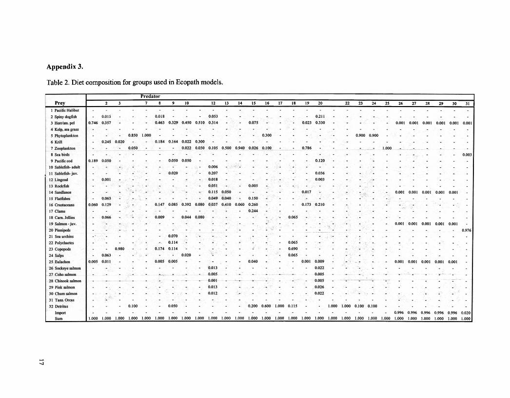
Appendix 3.

Table 2. Diet composition for groups used in Ecopath models.

PredatorPrey 2 7 8 9 10 12 Il 14 IS 16 17 18 19 20 22 23 24 25 26 27 28 29 30 31

I Pacific Halibut

2 Spiny dogfisb 0.Q15 0.018 0.053 0.211

3 Herr/sm. pel 0.746 0.357 0.463 0.329 0.450 0.510 0.314 0.075 0.023 0.330 0.001 0.001 0.001 0.001 0.001 0.001

4 Kelp. sea grass

5 Phytoplankton 0.850 1.000 0.300 0.900 0.900

6 Krill 0.245 0.020 0.184 0.164 0.022 0.300

7 Zooplankton 0.050 0.022 0.030 0.105 0.500 0.940 0.026 0.100 0.786 '-- -~--1.000

8 Sea birds 0.003

9 Pacific cod 0.189 0.050 0.050 0.050 0.120

10 Sablefish- adult 0.006 '",

11 Sablefish- juv. 0.020 0.207 0.036

12 Lingcod 0.001 0.018 0.003

13 RocIdisb 0.051 0.005

14 Sandlance;,..""

0.115 0.050 0.017 0.001 0.001 0.001 0.001 0.001, -:}.~:;.~IS Flatfisbes 0.063 0.049 0.040 0.150

16 Crustaceans 0.060 0.129 l',· 0.147 0.085 0.392 0.080 0.037 0.410 0.060 0.260 0.173 0.210

17 Clams 0.244

18 Cam. Jellies 0.066 0.009 0.044 0.080 0.065

19 Salmon - juv. .1 0.001 0.001 0.001 0.001 0.001~" '. ,

20 Pinnipeds 0.976

21 Sea urchins 0.070 .22 Polychaetes 0.114 .' 0.065

23 Copepods 0.980 0.174 0.114 0.690

24 Salps 0.063 0.020 0.065

25 Eulachon 0.005 0.011 0.005 0.005 0.040 0.001 0.009 .' . 0.001 0.001 0.001 0.001 0.001

26 Sockeye salmon 0.013 0.022

27 Coho salmon "-'0<- 0.005 0.005 - " .28 Chinook salmon 0.001 0.005 -------- . . .. . .29 Pink salmon 0.013 0.026

30 Chum salmon 0.012 0.022

31 Tans. Orcas ;..

32 Detritus 0.100 0.050 0.200 0.600 1.000 0.115 1.000 1.000 0.100 0.100

Import 0.996 0.996 0.996 0.996 0.996 0.020

Sum 1.000 1.000 1.000 1.000 1.000 1.000 1.000 1.000 1.000 1.000 1.000 1.000 1.600 1.000 1.000 1.000 1.000 1.000 1.000 1.000 1.000 1.000 1.000 1.000 1.000 1.000 1.000 1.000 1.000

Appendix 4. Ecopath model inputs and estimates.

Table 3. Basic input parameters for both of the Rivers Inlet models. The values in bold werecalculated by the Ecopath software. PIB is productionlbiomass, QIB is consumptionlbiomass, 01is the omnivory index, and EE is the ecotrophic efficiency, i.e., the proportion ofproduction thatis lost to predation mortality or fisheries catches.

Basic Parameters1990s Model 1950s Model

Group n me Trophic Biomas- PI B Q/B 01 EE Trophic Biomass PIB QIB 01 EElevcJ (1IkIli) Vyear) (/year) level (tfkm2) (/year) (/year)

Pacific H libLll 4.0 0.265 0..251 t.73 0.079 0.220 4.0 2.65 0.257 1.73 0.081 0.051Spil1Y dogfi.sh .6 4.5 0,_ - 0.262 0.873 3.6 4.75 0.2 5 0.267 0.970Herrlsm.. pt!1 .0 17.269 IA I 0.000 0.816 3.0 18.45 1.55 18 0.000 0.992KIp. SC<l grass 1.0 20. 4 0.000 0.000 1.0 20.3 4 0 0.000 0.000Ph opklllklon 1.0 154.6 200 () 0.000 0.190 1.0 154.64 200 0 0.000 0.190Krill ~.O ~.91 15 0.047 0.950 2.0 7.233 3 15 0.047 0.950:Zooplankloo 2.0 _0.289 33.5 lIU 0.000 0.044 2.0 26.289 33.5 111.5 0.000 0.080I'Sea birds .5 (J.OI .1 roo 0.245 0.059 3.5 0.023 0.1 100 0.245 0.058l'ociri 3.4 3.25 0.66- 3.3 0.373 0.978 3.4 4.875 0.665 3.3 0.376 0.986S~blc1ish- adult 3.6 0.1 ,I .73 0.230 0.408 3.6 0.15 0.1 3.73 0.230 0.827Sllblefish- juv. ! 3. \.5 .6 6.6 0.213 0.399 3.6 2.25 0.6 6.6 0.217 0.561Lingcod 4.1 .10- 0,8 0.293 0.965 4.1 0.525 0.8 3.3 0.279 0.150R c ·fi·h 3,] I. 16 0._ 3. 0.086 0.476 3.1 1.524 0.28 3.44 0.086 0.370:Sundlnnce 3.0 0.-95 2 1 0.001 0.191 3.0 0.595 2 18 0.001 0.446~Iatfi hes 3.1 - 1.15 .21 I 0.497 0.934 3.1 4.275 U5 3.21 0.505 0.798CrustllOl"m1S 2.1 15 1 to 0.090 0.337 2.1 16.8 2 10 0.090 0.405IClam.. l.G - L6 23 0.000 0.748 2.0 5.5 0.6 23 0.000 0.969iClimi 'orous Jellies 2.4 ,-9 .81 19.4 0.170 0.256 2.9 6.939 8.82 29.4 0.170 0.265Salm n· juvmiHt! J.t . 53 I 62, 0.040 0.003 3.1 0.653 6.018 62.8 0.065 0.017Pillnipeds 4.1 ..l5 .1_ 8.1 0.362 0.963 4.0 0.25 0.155 8.1 0.352 0.974Sea Uf hillS 2.0 2.4 3 .4 23 0.000 0.820 2.0 2.737 0.4 23 0.000 0.749PoJychactes 2,0 20 ) 3 . j 0.000 0.362 2.0 20 2 33.33 0.000 0.378Copepods '.0 ]6. 55 1!B.~3 0.000 0.487 2.0 16.7 55 183.33 0.000 0.510SaJps 2.0 5 12 0.000 0.984 2.0 5 3 12 0.000 0.988Eul:don 3.0 0.38 2 IS 0.000 0.949 3.0 1.9 2 18 0.000 0.270

ISockc}'e salmoOn - 0.709 1-32 13 0.036 0.553 3.5 3.545 1.332 13 0.036 0.542Coho lmon 3.5 O. lli 2.12- 13 I 0.036 0.849 3.5 0.1 2.125 13 0.036 0.841

I

Chinook salrnon 3.- 0, 45 OAI2 13 0.036 0.943 3.5 0.225 0.412 13 0.036 0.495Pink simon 3.- 0.1 9 1.25 0.036 0.923 3.5 0.545 1.255 13 0.036 0.535Chu.rn -salmon .3. _ O. 91 l-2.-2 I 0.036 0.933 3.5 0.785 1.55 13 0.036 0.995TailS. Orcas 5.1 I .02 7,4 0.009 0.000 5.0 0.004 0.02 lU 0.305 0.000D..:-tritus 1.0 - . - 0.113 0.045 1.0 154.64 - - 0:118 0.047

Appendix 5. Ecopath model outputs.

Table 4. The output statistics for both of the Rivers Inlet models. These outputs were calculatedby the Ecopath software.

Summar] statisticsParameter 1990s 1950s Units

Sum of all consumption 7777.882 7959.904 tlkm 2/yearSum of all exports 26846.832 26781.188 tlkm 2/yearSum of all respiratory flows 4215.936 4336.359 tlkm 2/yearSum of all flows into detritus 28120.412 28082.961 tlkm2/yearTotal system throughput 66961 67160 tlkm 2/yearSum of all production 33015 33041 tlkm 2/yearMean trophic level of the catch 3.67 3.83Gross efficiency (catch/net p.p.) 0.00003 0.000166Input total net primary production - - tlkm2/yearCalculated total net primary production 31009.199 31009.199Unaccounted primary production - -Total primary production/total respiration 7.355 7.151Net system production 26793.264 26672.84 tlkm 2/yearTotal primary production/total biomass 99.307 93.907Total biomass/total throughput 0.005 0.005Total biomass (excluding detritus) 312.254 330.212 tlkm2

Total catches 0.938 5.154 tlkm2/year

Connectance Index 0.134 0.134System Omnivory Index 0.089 0.088

lQ

mon

In

J1

Il

L..----. '-' Eoo Coho selmon .' "-:-'- Chum'"nill~lmon

Paclnc Halibut ChJn~lmO , Pln~~onl- i..--, .. '---'~

r--

~I [lJJ-r-

- It-- SPln~n.h,----, sabl~~adult Sable.!!;~llNSa" birds

~=- --4~ Paclnccod ~I

nL Rocknsh

-r I- .k II FI~~e. -

Selmon - juvenllla '"'"'~.:ll-

~Ton cllmlv9Jellies SIl~I~ce Harr~m~1

r

- ....I T q bchelte.

LJse~ln.

-1----0~ Cru.!!,.~.n.Krill

CO~~.lams

21- '-lr- Zoopl.!'kton~~ L...,

-IIii

.... ,I 'l

,.--,

. Ta.J8'0rcas

-I,oiJ;:roIo:lI<Q

Figure 6 Diagram of food web for the 1990s Ecopath model showing the trophic interactions. The box size is proportional to the biomass of thegroup. The group production leaves the top of the box and the consumption enters the bottom.