ch02 perloff 16073 - wps.aw.comwps.aw.com/wps/media/objects/591/605493/protected/ch02/ch02.pdf ·...

13

In this chapter,

we examine

six main

topics

Supply and Demand

Talk is cheap because supply exceeds demand.

When asked, “What is the most important thing you know about economics?”many people reply, “Supply equals demand.” This statement is a shorthand descrip-tion of one of the simplest yet most powerful models of economics. The supply-and-demand model describes how consumers and suppliers interact to determine thequantity of a good or service sold in a market and the price at which it is sold. Touse the model, you need to determine three things: buyers’ behavior, sellers’ behav-ior, and how they interact. After reading this chapter, you should be adept enoughat using the supply-and-demand model to analyze some of the most important pol-icy questions facing your country today, such as those concerning internationaltrade, minimum wages, and price controls on health care.

After reading that grandiose claim, you may ask, “Is that all there is to eco-nomics? Can I become an expert economist that fast?” The answer to both thesequestions is no (of course). In addition, you need to learn the limits of this modeland what other models to use when this one does not apply. (You must also learnthe economists’ secret handshake.)

Even with its limitations, the supply-and-demand model is the most widely usedeconomic model. It provides a good description of how many markets function andworks particularly well in markets in which there are many buyers and many sell-ers, such as in most agriculture and labor markets. Like all good theories, the sup-ply-and-demand model can be tested—and possibly shown to be false. But inmarkets where it is applicable, it allows us to make accurate predictions easily.

1. Demand: The quantity of a good or service that consumers demand depends onprice and other factors such as consumers’ incomes and the price of related goods.

2. Supply: The quantity of a good or service that firms supply depends on price andother factors such as the cost of inputs firms use to produce the good or service.

3. Market equilibrium: The interaction between consumers’ demand and firms’ sup-ply determines the market price and quantity of a good or service that is bought andsold.

4. Shocking the equilibrium: Changes in a factor that affect demand (such as con-sumer’s income), supply (such as a rise in the price of inputs), or a new governmentpolicy (such as a new tax) alter the market price and quantity of a good.

5. Effects of government interventions: Government policies may alter the equilibriumand cause the quantity supplied to differ from the quantity demanded.

6. When to use the supply-and-demand model: The supply-and-demand model appliesonly to competitive markets.

2C H A P T E R

CHAPTER 2 Supply and Demand14

Potential consumers decide how much of a good or service to buy on the basis of itsprice and many other factors, including their own tastes, information, prices ofother goods, income, and government actions. Before concentrating on the role ofprice in determining demand, let’s look briefly at some of the other factors.

Consumers’ tastes determine what they buy. Consumers do not purchase foodsthey dislike, artwork they hate, or clothes they view as unfashionable or uncom-fortable. Advertising may influence peoples’ tastes.

Similarly, information (or misinformation) about the uses of a good affects con-sumers’ decisions. A few years ago when many consumers were convinced that oat-meal could lower their cholesterol level, they rushed to grocery stores and boughtlarge quantities of oatmeal. (They even ate some of it until they remembered thatthey couldn’t stand how it tastes.)

The prices of other goods also affect consumers’ purchase decisions. Beforedeciding to buy Levi’s jeans, you might check the prices of other brands. If the priceof a close substitute—a product that you view as similar or identical to the one youare considering purchasing—is much lower than the price of Levi’s jeans, you maybuy that brand instead. Similarly, the price of a complement—a good that you liketo consume at the same time as the product you are considering buying—may affectyour decision. If you eat pie only with ice cream, the higher the price of ice cream,the less likely you are to buy pie.

Income plays a major role in determining what and how much to purchase.People who suddenly inherit great wealth may purchase a Rolls-Royce or other lux-ury items and would probably no longer buy do-it-yourself repair kits.

Government rules and regulations affect purchase decisions. Sales taxes increasethe price that a consumer must spend for a good, and government-imposed limitson the use of a good may affect demand. If a city’s government bans the use of skate-boards on its streets, skateboard sales fall.

Other factors may also affect the demand for specific goods. Consumers are morelikely to have telephones if most of their friends have telephones. The demand forsmall, dead evergreen trees is substantially higher in December than at other timesof the year.

Dr. David A. Kessler, former U.S. Commissioner of Food and Drugs, alleged thatBrown & Williamson Tobacco Corporation developed a genetically engineeredtobacco with more than double the amount of nicotine that some other cigarettesdeliver to the smoker. Higher levels of nicotine may increase smokers’ addiction andthus boost the demand for cigarettes.

Although many factors influence demand, economists usually concentrate onhow price affects the quantity demanded. The relationship between price and quan-tity demanded plays a critical role in determining the market price and quantity ina supply-and-demand analysis. To determine how a change in price affects the quan-tity demanded, economists must hold constant other factors such as income andtastes that affect demand.

2.1 DEMAND

Demand 15

The amount of a good that consumers are willing to buy at a given price, holding con-stant the other factors that influence purchases, is the quantity demanded. The quan-tity demanded of a good or service can exceed the quantity actually sold. For example,as a promotion, a local store might sell music CDs for $1 each today only. At that lowprice, you might want to buy 25 CDs, but because the store ran out of stock, you canbuy only 10 CDs. The quantity you demand is 25—it’s the amount you want, eventhough the amount you actually buy is only 10.

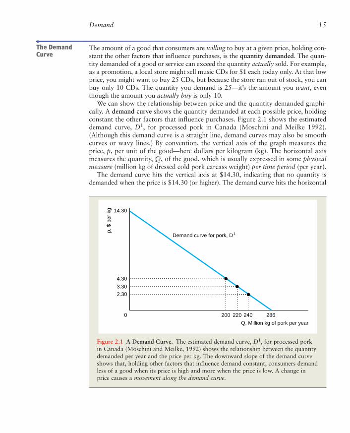
We can show the relationship between price and the quantity demanded graphi-cally. A demand curve shows the quantity demanded at each possible price, holdingconstant the other factors that influence purchases. Figure 2.1 shows the estimateddemand curve, D1, for processed pork in Canada (Moschini and Meilke 1992).(Although this demand curve is a straight line, demand curves may also be smoothcurves or wavy lines.) By convention, the vertical axis of the graph measures theprice, p, per unit of the good—here dollars per kilogram (kg). The horizontal axismeasures the quantity, Q, of the good, which is usually expressed in some physicalmeasure (million kg of dressed cold pork carcass weight) per time period (per year).

The demand curve hits the vertical axis at $14.30, indicating that no quantity isdemanded when the price is $14.30 (or higher). The demand curve hits the horizontal

The DemandCurve

Figure 2.1 A Demand Curve. The estimated demand curve, D1, for processed porkin Canada (Moschini and Meilke, 1992) shows the relationship between the quantitydemanded per year and the price per kg. The downward slope of the demand curveshows that, holding other factors that influence demand constant, consumers demandless of a good when its price is high and more when the price is low. A change inprice causes a movement along the demand curve.

p, $

per

kg

200 220

Demand curve for pork, D1

240 286

Q, Million kg of pork per year

0

2.303.30

4.30

14.30

16 CHAPTER 2 Supply and Demand

quantity axis at 286 million kg—the amount of pork that consumers want if the priceis zero. To find out what quantity is demanded at a price between these extremes, pickthat price on the vertical axis—say, $3.30 per kg—draw a horizontal line across untilyou hit the demand curve, and then draw a line straight down to the horizontal quan-tity axis: 220 million kg of pork per year is demanded at that price.

One of the most important things to know about a graph of a demand curve iswhat is not shown. All relevant economic variables that are not explicitly shown onthe demand curve graph—tastes, information, prices of other goods (such as beefand chicken), income of consumers, and so on—are held constant. Thus the demandcurve shows how quantity varies with price but not how quantity varies with tastes,information, the price of substitute goods, or other variables.1

Effect of Prices on the Quantity Demanded. Many economists claim that the mostimportant empirical finding in economics is the Law of Demand: Consumers demandmore of a good the lower its price, holding constant tastes, the prices of other goods,and other factors that influence the amount they consume. According to the Law ofDemand, demand curves slope downward, as in Figure 2.1.2

A downward-sloping demand curve illustrates that consumers demand more ofthis good when its price is lower and less when its price is higher. What happens tothe quantity of pork demanded if the price of pork drops and all other variablesremain constant? If the price of pork falls by $1 from $3.30 to $2.30 in Figure 2.1,the quantity consumers want to buy increases from 220 to 240.3 Similarly, if theprice increases from $3.30 to $4.30, the quantity consumers demand decreases from220 to 200. These changes in the quantity demanded in response to changes in priceare movements along the demand curve. Thus the demand curve is a concise sum-mary of the answers to the question “What happens to the quantity demanded asthe price changes, when all other factors are held constant?”

Effects of Other Factors on Demand. If a demand curve measures the effects of pricechanges when all other factors that affect demand are held constant, how can we usedemand curves to show the effects of a change in one of these other factors, such as

1Because prices, quantities, and other factors change simultaneously over time, economists usestatistical techniques to hold the effects of factors other than the price of the good constant sothat they can determine how price affects the quantity demanded. (See Appendix 2A.) Moschiniand Meilke (1992) used such techniques to estimate the pork demand curve. As with any esti-mate, their estimates are probably more accurate in the observed range of prices ($1 to $6 perkg) than at very high or very low prices.

2Theoretically, a demand curve could slope upward (Chapter 5); however, available empiricalevidence strongly supports the Law of Demand.

3Economists, being lazy, typically do not state the relevant physical and time period measuresunless they are particularly useful. They refer to quantity rather than something useful suchas “metric tons per year” and price rather than “cents per pound.” Being as lazy as the nexteconomist, I’ll follow this sloppy convention when no confusion is likely to arise. To keep fromdriving us all nuts, from here on, I’ll usually refer to the price as $3.30 (with the “per kg”understood) and the quantity as 220 (with the “million kg per year” understood).

Demand 17

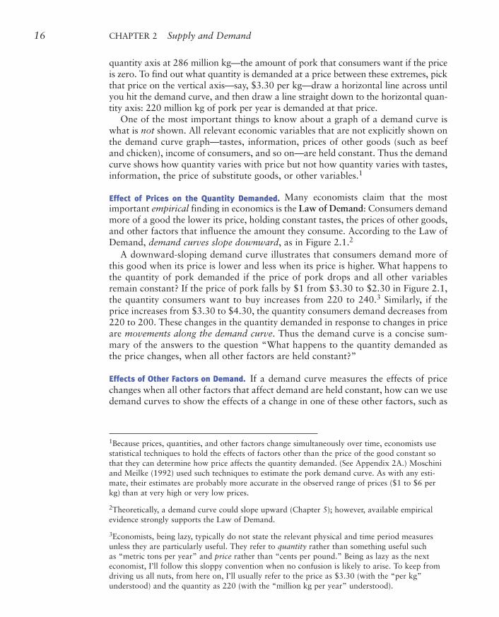
Figure 2.2 A Shift of the Demand Curve. The demand curve for processed porkshifts to the right from D1 to D2 as the price of beef rises from $4 to $4.60. As aresult of the increase in beef prices, more pork is demanded at any given price.

p, $

per

kg

220176

Effect of a 60¢ increase in the price of beef

D1

D 2

232


0

3.30

the price of beef? One solution is to draw the demand curve in a three-dimensionaldiagram with the price of pork on one axis, the price of beef on a second axis, andthe quantity of pork on the third axis. But just thinking about drawing such a dia-gram probably makes your head hurt.

Economists use a simpler approach to show the effect on demand of a change ina factor that affects demand other than the price of the good. A change in any fac-tor other than price of the good itself causes a shift of the demand curve rather thana movement along the demand curve.

Many people view beef as a close substitute for pork. Thus at a given price ofpork, if the price of beef rises, some people will switch from beef to pork. Figure 2.2shows how the demand curve for pork shifts to the right from the original demandcurve D1 to a new demand curve D2 as the price of beef rises from $4.00 to $4.60per kg. (The quantity axis starts at 176 instead of 0 in the figure to emphasize therelevant portion of the demand curve.) On the new demand curve, D2, more porkis demanded at any given price than on D1. At a price of pork of $3.30, the quan-tity of pork demanded goes from 220 on D1, before the change in the price of beef,to 232 on D2, after the price change.

Similarly, a change in information can shift the demand curve. The average num-ber of eggs per year each American eats has fallen steadily since World War II, eventhough the price of eggs has fallen relative to the price of other goods during thisperiod. Brown and Schrader (1990) found that new information about the linkbetween cholesterol (eggs are high in cholesterol) and heart disease caused thedemand curve for eggs to shift to the left. This shift was largely responsible for theU.S. per capita decline in fresh egg consumption of 36% from 1945 to 2001.


4The numbers are rounded slightly from the estimates to simplify the calculation. For example,the estimate of the coefficient on the price of beef is 19.5, not 20, as the equation shows.

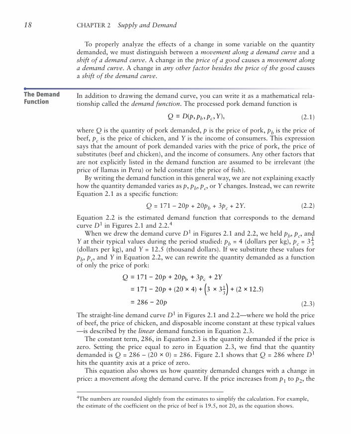
To properly analyze the effects of a change in some variable on the quantitydemanded, we must distinguish between a movement along a demand curve and ashift of a demand curve. A change in the price of a good causes a movement alonga demand curve. A change in any other factor besides the price of the good causesa shift of the demand curve.

In addition to drawing the demand curve, you can write it as a mathematical rela-tionship called the demand function. The processed pork demand function is

(2.1)

where Q is the quantity of pork demanded, p is the price of pork, pb is the price ofbeef, pc is the price of chicken, and Y is the income of consumers. This expressionsays that the amount of pork demanded varies with the price of pork, the price ofsubstitutes (beef and chicken), and the income of consumers. Any other factors thatare not explicitly listed in the demand function are assumed to be irrelevant (theprice of llamas in Peru) or held constant (the price of fish).

By writing the demand function in this general way, we are not explaining exactlyhow the quantity demanded varies as p, pb, pc, or Y changes. Instead, we can rewriteEquation 2.1 as a specific function:

Q = 171 – 20p + 20pb + 3pc + 2Y. (2.2)

Equation 2.2 is the estimated demand function that corresponds to the demandcurve D1 in Figures 2.1 and 2.2.4

When we drew the demand curve D1 in Figures 2.1 and 2.2, we held pb, pc, andY at their typical values during the period studied: pb = 4 (dollars per kg), pc = 3(dollars per kg), and Y = 12.5 (thousand dollars). If we substitute these values forpb, pc, and Y in Equation 2.2, we can rewrite the quantity demanded as a functionof only the price of pork:

(2.3)

The straight-line demand curve D1 in Figures 2.1 and 2.2—where we hold the priceof beef, the price of chicken, and disposable income constant at these typical values—is described by the linear demand function in Equation 2.3.

The constant term, 286, in Equation 2.3 is the quantity demanded if the price iszero. Setting the price equal to zero in Equation 2.3, we find that the quantitydemanded is Q = 286 – (20 × 0) = 286. Figure 2.1 shows that Q = 286 where D1

hits the quantity axis at a price of zero.This equation also shows us how quantity demanded changes with a change in

price: a movement along the demand curve. If the price increases from p1 to p2, the

Q p p p Y

p

p

= − + + +

= − + × + ×( ) + ×

= −

171 20 20 3 2

171 20 20 4 3 3 2 12 5

286 20

13

b c

( ) ( . )

13

Q D p p p Yb c= ( , , , ),

The DemandFunction

Demand 19

change in price, ∆p, equals p2 – p1. (The ∆ symbol, the Greek letter delta, means“change in” the following variable, so ∆p means “change in price.”) As Figure 2.1illustrates, if the price of pork increases by $1 from p1 = $3.30 to p2 = $4.30, ∆p =$1 and ∆Q = Q2 – Q1 = 200 – 220 = –20 million kg per year.

More generally, the quantity demanded at p1 is Q1 = D(p1), and the quantitydemanded at p2 is Q2 = D(p2). The change in the quantity demanded, ∆Q = Q2 – Q1,in response to the price change (using Equation 2.3) is

Thus the change in the quantity demanded, ∆Q, is –20 times the change in the price,∆p. If ∆p = $1, ∆Q = –20∆p = –20.

The slope of a demand curve is ∆p/∆Q, the “rise” (∆p, the change along the ver-tical axis) divided by the “run” (∆Q, the change along the horizontal axis). Theslope of demand curve D1 in Figures 2.1 and 2.2 is

The negative sign of this slope is consistent with the Law of Demand. The slope saysthat the price rises by $1 per kg as the quantity demanded falls by 20 million kg peryear. Turning that statement around: The quantity demanded falls by 20 million kgper year as the price rises by $1 per kg.

Thus we can use the demand curve to answer questions about how a change inprice affects the quantity demanded and how a change in the quantity demandedaffects price. We can also answer these questions using demand functions.

To answer the question about how a change in quantity affects price, we use alge-bra to rewrite Equation 2.3 so that price is a function of quantity. We call thisrewritten demand curve an inverse demand curve. Subtracting Q from both sides ofEquation 2.3 and adding 20p to both sides, we find that 20p = 286 – Q. Dividingboth sides of the equation by 20, we obtain the inverse demand function:

p = 14.30 – 0.05Q. (2.4)

Equation 2.4 shows that if the quantity increases by ∆Q, price falls by ∆p = –0.05∆Q (where –0.05 is the number multiplied by Q in the equation).5 For consumersto demand one million more kg of pork per year, the price must fall by nearly 5¢ akg, which is a movement along the demand curve.

Slope riserun

$1 per kg20 million kg per year

0.05 per million kg per year.

= = =−

= −

∆∆

pQ

$

∆

∆

Q Q Q

D p D p

p p

p p

p

= −

= −

= − − −

= − −

= −

2 1

2 1

2 1

2 1

286 20 286 20

20

20

( ) ( )

( ) ( )

( )

.

5Let the quantity increase from Q1 to Q2 so that ∆Q = Q2 – Q1. The change in price is ∆p = p2 – p1:

∆p = (14.30 – 0.05Q2) – (14.30 – 0.05Q1) = –0.05(Q2 – Q1) = –0.05∆Q.


AGGREGATING THE DEMAND FOR CLING PEACHES

We illustrate how to combine individual demand curves to get a totaldemand curve graphically using estimated demand curves for cling peaches(French and King, 1986). Cling peaches are used for canning. The total

p, $

per

ton

50

Q, Tons of peaches per 10,000 people per year

0

275

183

Total demand

Demand for canned peaches

Demand for fruit cocktail

Qc = 18 Q = 22Qf = 4

If we know the demand curve for each of two consumers, how do we determine thetotal demand for the two consumers combined? The total quantity demanded at agiven price is the sum of the quantity each consumer demands at that price.

We can use the demand functions to determine the total demand of several con-sumers. Suppose that the demand function for Consumer 1 is

Q1 = D1(p)

and the demand function for Consumer 2 is

Q2 = D2(p).

At price p, Consumer 1 demands Q1 units, Consumer 2 demands Q2 units, and thetotal demand of both consumers is the sum of the quantities each demands separately:

Q = Q1 + Q2 = D1(p) + D2(p).

We can generalize this approach to look at the total demand for three or more con-sumers.

It makes sense to add the quantities demanded only when all consumers face thesame price. Adding the quantity Consumer 1 demands at one price to the quantityConsumer 2 demands at another price would be like adding apples and oranges.

SummingDemandCurves

Application

Supply 21

Knowing how much consumers want is not enough, by itself, to tell us what price andquantity are observed in a market. To determine the market price and quantity, wealso need to know how much firms want to supply at any given price.

Firms determine how much of a good to supply on the basis of the price of thatgood and other factors, including the costs of production and government rulesand regulations. Usually, we expect firms to supply more at a higher price. Beforeconcentrating on the role of price in determining supply, we’ll briefly describe therole of some of the other factors.

Costs of production affect how much firms want to sell of a good. As a firm’s costfalls, it is willing to supply more, all else the same. If the firm’s cost exceeds what itcan earn from selling the good, the firm sells nothing. Thus, factors that affect costs,also affect supply. A technological advance that allows a firm to produce a good atlower cost leads the firm to supply more of that good, all else the same.

Government rules and regulations affect how much firms want to sell or areallowed to sell. Taxes and many government regulations—such as those coveringpollution, sanitation, and health insurance—alter the costs of production. Otherregulations affect when and how the product can be sold. In Germany, retailers maynot sell most goods and services on Sundays or during evening hours. In the UnitedStates, the sale of cigarettes and liquor to children is prohibited. New York, SanFrancisco, and many other cities restrict the number of taxicabs.

The quantity supplied is the amount of a good that firms want to sell at a givenprice, holding constant other factors that influence firms’ supply decisions, suchas costs and government actions. We can show the relationship between price andthe quantity supplied graphically. A supply curve shows the quantity supplied ateach possible price, holding constant the other factors that influence firms’ supplydecisions. Figure 2.3 shows the estimated supply curve, S1, for processed pork(Moschini and Meilke, 1992). As with the demand curve, the price on the verticalaxis is measured in dollars per physical unit (dollars per kg), and the quantity onthe horizontal axis is measured in physical units per time period (millions of kgper year). Because we hold fixed other variables that may affect the supply, suchas costs and government rules, the supply curve concisely answers the question“What happens to the quantity supplied as the price changes, holding all otherfactors constant?”

2.2 SUPPLY

demand for cling peaches in the figure is the sum of the demand for clingpeaches for use in cans of peaches and the demand for cling peaches for usein cans of fruit cocktail.

Farmers sold cling peaches for $183 per ton in 1984. At that price, fruitcocktail canners demanded Qf = 4 tons per 10,000 consumers per yearand peach canners demanded Qc = 18, so the total quantity demanded wasQ = Qf + Qc = 4 + 18 = 22.

The SupplyCurve


p, $

per

kg

220176

Supply curve, S1

300


0

3.30

5.30

Figure 2.3 A Supply Curve. The estimated supply curve, S1, for processed pork inCanada (Moschini and Meilke, 1992) shows the relationship between the quantitysupplied per year and the price per kg, holding cost and other factors that influencesupply constant. The upward slope of this supply curve indicates that firms supplymore of this good when its price is high and less when the price is low. An increasein the price of pork causes a movement along the supply curve, resulting in a largerquantity of pork supplied.

Effect of Price on Supply. We illustrate how price affects the quantity supplied usingthe supply curve for processed pork in Figure 2.3. The supply curve for pork isupward sloping. As the price of pork increases, firms supply more. If the price is$3.30, the market supplies a quantity of 220 (million kg per year). If the price risesto $5.30, the quantity supplied rises to 300. An increase in the price of pork causesa movement along the supply curve, resulting in more pork being supplied.

Although the Law of Demand requires that the demand curve slope downward,there is no “Law of Supply” that requires the market supply curve to have a partic-ular slope. The market supply curve can be upward sloping, vertical, horizontal, ordownward sloping. Many supply curves slope upward, such as the one for pork.Along such supply curves, the higher the price, the more firms are willing to sell,holding costs and government regulations fixed.

Effects of Other Variables on Supply. A change in a variable other than the price ofpork causes the entire supply curve to shift. Suppose the price, ph, of hogs—the mainfactor used to produce processed pork—increases from $1.50 per kg to $1.75 perkg. Because it is now more expensive to produce pork, the supply curve shifts to the

Supply 23

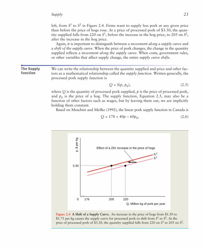
left, from S1 to S2 in Figure 2.4. Firms want to supply less pork at any given pricethan before the price of hogs rose. At a price of processed pork of $3.30, the quan-tity supplied falls from 220 on S1, before the increase in the hog price, to 205 on S2,after the increase in the hog price.

Again, it is important to distinguish between a movement along a supply curve anda shift of the supply curve. When the price of pork changes, the change in the quantitysupplied reflects a movement along the supply curve. When costs, government rules,or other variables that affect supply change, the entire supply curve shifts.

We can write the relationship between the quantity supplied and price and other fac-tors as a mathematical relationship called the supply function. Written generally, theprocessed pork supply function is

Q = S(p, ph), (2.5)

where Q is the quantity of processed pork supplied, p is the price of processed pork,and ph is the price of a hog. The supply function, Equation 2.5, may also be afunction of other factors such as wages, but by leaving them out, we are implicitlyholding them constant.

Based on Moschini and Meilke (1992), the linear pork supply function in Canada is

Q = 178 + 40p – 60ph, (2.6)

Figure 2.4 A Shift of a Supply Curve. An increase in the price of hogs from $1.50 to$1.75 per kg causes the supply curve for processed pork to shift from S1 to S2. At theprice of processed pork of $3.30, the quantity supplied falls from 220 on S1 to 205 on S2.

p, $

per

kg

205176

Effect of a 25¢ increase in the price of hogs

S1S 2

220


0

3.30

The SupplyFunction


6Substituting ph = $1.50 into Equation 2.6, we find that

Q = 178 + 40p – 60ph = 178 + 40p – (60 × 1.50) = 88 + 40p.

7As the price increases from p1 to p2, the quantity supplied goes from Q1 to Q2, so the change inquantity supplied, ∆Q = Q2 – Q1, is

∆Q = (88 + 40p2) – (88 + 40p1) = 40(p2 – p1) = 40∆p.

where quantity is in millions of kg per year and the prices are in Canadian dollarsper kg. If we hold the price of hogs fixed at its typical value of $1.50 per kg, we canrewrite the supply function in Equation 2.6 as6

Q = 88 + 40p. (2.7)

What happens to the quantity supplied if the price of processed pork increasesby ∆p = p2 – p1? Using the same approach as before, we learn from Equation 2.7that ∆Q = 40∆p.7 A $1 increase in price (∆p = 1) causes the quantity supplied toincrease by ∆Q = 40 million kg per year. This change in the quantity of pork sup-plied as p increases is a movement along the supply curve.

The total supply curve shows the total quantity produced by all suppliers at eachpossible price. For example, the total supply of rice in Japan is the sum of thedomestic and foreign supply curves of rice.

Suppose that the domestic supply curve (panel a) and foreign supply curve (panelb) of rice in Japan are as Figure 2.5 shows. The total supply curve, S in panel c, isthe horizontal sum of the Japanese domestic supply curve, Sd, and the foreign sup-ply curve, Sf. In the figure, the Japanese and foreign supplies are zero at any priceequal to or less than p

–, so the total supply is zero. At prices above p

–, the Japanese

and foreign supplies are positive, so the total supply is positive. For example, whenprice is p*, the quantity supplied by Japanese firms is Q*d (panel a), the quantity sup-plied by foreign firms is Q*f (panel b), and the total quantity supplied is Q* = Q*d +Q*f (panel c). Because the total supply curve is the horizontal sum of the domesticand foreign supply curves, the total supply curve is flatter than either of the other twosupply curves.

We can use this approach for deriving the total supply curve to analyze the effect ofgovernment policies on the total supply curve. Traditionally, the Japanese govern-ment banned the importation of foreign rice. We want to determine how much lessis supplied at any given price to the Japanese market because of this ban.

Without a ban, the foreign supply curve is Sf in panel b of Figure 2.5. A ban onimports eliminates the foreign supply, so the foreign supply curve after the ban isimposed, Sf

–, is a vertical line at Qf = 0. The import ban has no effect on the domes-

tic supply curve, Sd, so the supply curve is the same as in panel a.

SummingSupply Curves

Effects ofGovernmentImportPolicies onSupply Curves

Supply 25

Because the foreign supply with a ban, Sf–

, is zero at every price, the total supplywith a ban, S

–, in panel c is the same as the Japanese domestic supply, Sd, at any given

price. The total supply curve under the ban lies to the left of the total supply curvewithout a ban, S. Thus the effect of the import ban is to rotate the total supply curvetoward the vertical axis.

The limit that a government sets on the quantity of a foreign-produced good thatmay be imported is called a quota. By absolutely banning the importation of rice,the Japanese government sets a quota of zero on rice imports. Sometimes govern-ments set positive quotas, Q

–> 0. The foreign firms may supply as much as they

want, Qf, as long as they supply no more than the quota: Qf ≤ Q–

.We investigate the effect of such a quota in Solved Problem 2.1. In most of the

solved problems in this book, you are asked to determine how a change in a vari-able or policy affects one or more variables. In this problem, the policy changesfrom no quota to a quota, which affects the total supply curve.

Figure 2.5 Total Supply: The Sum of Domesticand Foreign Supply. If foreigners may sell theirrice in Japan, the total Japanese supply of rice,S, is the horizontal sum of the domestic Japanesesupply, Sd, and the imported foreign supply,

Sf. With a ban on foreign imports, the foreign sup-ply curve, Sf– , is zero at every price, so the total sup-ply curve, S

–, is the same as the domestic supply

curve, Sd.

p, P

rice

per

ton

p, P

rice

per

ton

p, P

rice

per

ton

Qd*

S d S f (ban)

Qf* Q = Qd

* Q* = Qd* + Qf

*

Qd, Tons per year Qf , Tons per year Q, Tons per year

(a) Japanese Domestic Supply (b) Foreign Supply (c) Total Supply

p* p* p*

—S (ban)—

S (no ban)S f (no ban)

p—

p—

p—

How does a quota set by the United States on foreign steel imports of Q–

affect the

total American supply curve for steel given the domestic supply, Sd in panel a of the

graph, and foreign supply, Sf in panel b?

Solved Problem 2.1

prob025.html


Answer

1. Determine the American supply curve without the quota: The no-quotatotal supply curve, S in panel c, is the horizontal sum of the U.S. domes-tic supply curve, Sd, and the no-quota foreign supply curve, Sf.

2. Show the effect of the quota on foreign supply: At prices less than p–, for-eign suppliers want to supply quantities less than the quota, Q

–. As a result,

the foreign supply curve under the quota, Sf–, is the same as the no-quota

foreign supply curve, Sf, for prices less than p–. At prices above p–, foreignsuppliers want to supply more but are limited to Q

–. Thus the foreign sup-

ply curve with a quota, Sf–, is vertical at Q

–for prices above p–.

3. Determine the American total supply curve with the quota: The total sup-ply curve with the quota, S

–, is the horizontal sum of Sd and Sf–

. At any priceabove p–, the total supply equals the quota plus the domestic supply. Forexample at p*, the domestic supply is Q*d and the foreign supply is Q

–f, so

the total supply is Q*d + Q–

f. Above p–, S–

is the domestic supply curve shiftedQ–

units to the right. As a result, the portion of S–

above p– has the sameslope as Sd.

4. Compare the American total supply curves with and without the quota:At prices less than or equal to p–, the same quantity is supplied with andwithout the quota, so S

–is the same as S. At prices above p–, less is supplied

with the quota than without one, so S–

is steeper than S, indicating that agiven increase in price raises the quantity supplied by less with a quotathan without one.

p, P

rice

per

ton

p, P

rice

per

ton

p, P

rice

per

ton

S d

Q, Tons per year

(a) U.S. Domestic Supply (b) Foreign Supply (c) Total Supply

p* p* p*

p— p— p—

S—

S

Qd—

Qf—

Qd, Tons per year Qf , Tons per year

Qd* Qf

*

S f—

S f

Qd* + Qf

*—Qd

* + Qf——

Qd + Qf

Market Equilibrium 27

The supply and demand curves determine the price and quantity at which goodsand services are bought and sold. The demand curve shows the quantitiesconsumers want to buy at various prices, and the supply curve shows the quanti-ties firms want to sell at various prices. Unless the price is set so that consumerswant to buy exactly the same amount that suppliers want to sell, either somebuyers cannot buy as much as they want or some sellers cannot sell as much asthey want.

When all traders are able to buy or sell as much as they want, we say that themarket is in equilibrium: a situation in which no participant wants to change itsbehavior. A price at which consumers can buy as much as they want and sellers cansell as much as they want is called an equilibrium price. The quantity that is boughtand sold at the equilibrium price is called the equilibrium quantity.

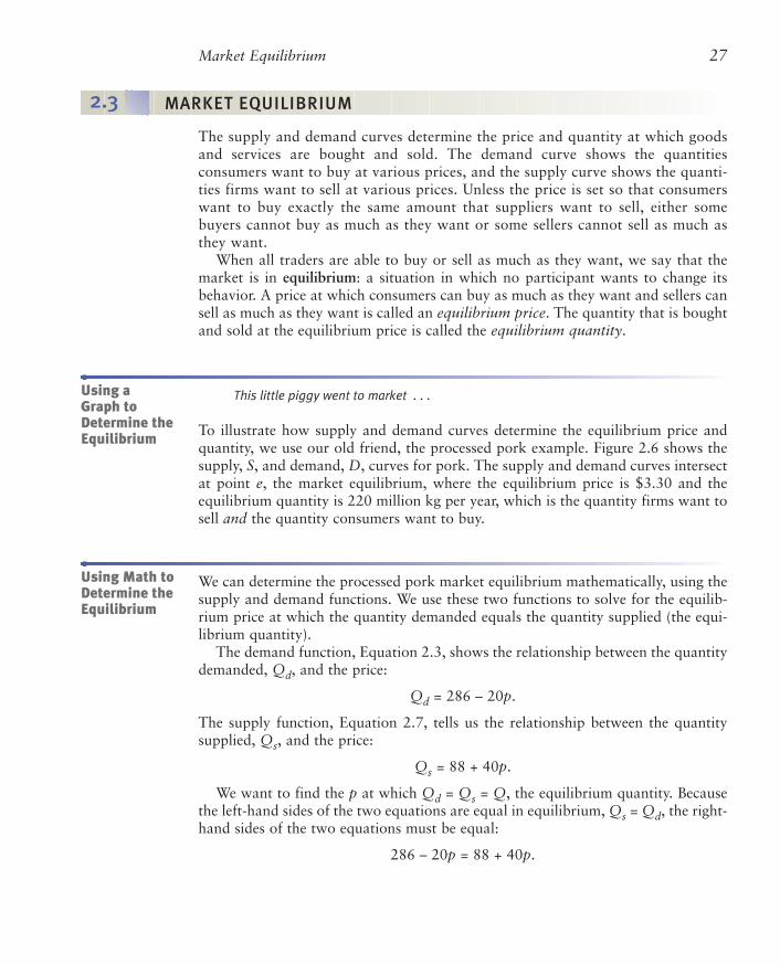
This little piggy went to market . . .

To illustrate how supply and demand curves determine the equilibrium price andquantity, we use our old friend, the processed pork example. Figure 2.6 shows thesupply, S, and demand, D, curves for pork. The supply and demand curves intersectat point e, the market equilibrium, where the equilibrium price is $3.30 and theequilibrium quantity is 220 million kg per year, which is the quantity firms want tosell and the quantity consumers want to buy.

We can determine the processed pork market equilibrium mathematically, using thesupply and demand functions. We use these two functions to solve for the equilib-rium price at which the quantity demanded equals the quantity supplied (the equi-librium quantity).

The demand function, Equation 2.3, shows the relationship between the quantitydemanded, Qd, and the price:

Qd = 286 – 20p.

The supply function, Equation 2.7, tells us the relationship between the quantitysupplied, Qs, and the price:

Qs = 88 + 40p.

We want to find the p at which Qd = Qs = Q, the equilibrium quantity. Becausethe left-hand sides of the two equations are equal in equilibrium, Qs = Qd, the right-hand sides of the two equations must be equal:

286 – 20p = 88 + 40p.

Using aGraph toDetermine theEquilibrium

Using Math toDetermine theEquilibrium

2.3 MARKET EQUILIBRIUM


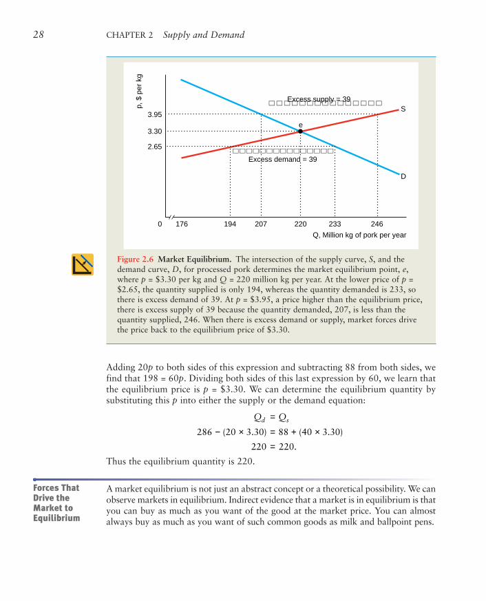
Figure 2.6 Market Equilibrium. The intersection of the supply curve, S, and thedemand curve, D, for processed pork determines the market equilibrium point, e,where p = $3.30 per kg and Q = 220 million kg per year. At the lower price of p =$2.65, the quantity supplied is only 194, whereas the quantity demanded is 233, sothere is excess demand of 39. At p = $3.95, a price higher than the equilibrium price,there is excess supply of 39 because the quantity demanded, 207, is less than thequantity supplied, 246. When there is excess demand or supply, market forces drivethe price back to the equilibrium price of $3.30.

p, $

per

kg

220176

D

S

e

233 246194 207


0

3.95

3.30

2.65

Excess supply = 39

Excess demand = 39

Adding 20p to both sides of this expression and subtracting 88 from both sides, wefind that 198 = 60p. Dividing both sides of this last expression by 60, we learn thatthe equilibrium price is p = $3.30. We can determine the equilibrium quantity bysubstituting this p into either the supply or the demand equation:

Thus the equilibrium quantity is 220.

A market equilibrium is not just an abstract concept or a theoretical possibility. We canobserve markets in equilibrium. Indirect evidence that a market is in equilibrium is thatyou can buy as much as you want of the good at the market price. You can almostalways buy as much as you want of such common goods as milk and ballpoint pens.

Q Qd s=

− × = + ×=

286 20 3 30 88 40 3 30

220 220

( . ) ( . )

.

Forces ThatDrive theMarket toEquilibrium

anim028.html

Market Equilibrium 29

Amazingly, a market equilibrium occurs without any explicit coordinationbetween consumers and firms. In a competitive market such as that for agriculturalgoods, millions of consumers and thousands of firms make their buying and sell-ing decisions independently. Yet each firm can sell as much as it wants; eachconsumer can buy as much as he or she wants. It is as though an unseen marketforce, like an invisible hand, directs people to coordinate their activities to achievea market equilibrium.

What really causes the market to move to an equilibrium? If the price is not atthe equilibrium level, consumers or firms have an incentive to change their behav-ior in a way that will drive the price to the equilibrium level, as we now illustrate.

If the price were initially lower than the equilibrium price, consumers wouldwant to buy more than suppliers want to sell. If the price of pork is $2.65 in Figure2.6, firms are willing to supply 194 million kg per year but consumers demand 233million kg. At this price, the market is in disequilibrium, meaning that the quantitydemanded is not equal to the quantity supplied. There is excess demand—theamount by which the quantity demanded exceeds the quantity supplied at a speci-fied price—of 39 (= 233 – 194) million kg per year at a price of $2.65.

Some consumers are lucky enough to buy the pork at $2.65. Other consumerscannot find anyone who is willing to sell them pork at that price. What can they do?Some frustrated consumers may offer to pay suppliers more than $2.65.Alternatively, suppliers, noticing these disappointed consumers, may raise theirprices. Such actions by consumers and producers cause the market price to rise. Asthe price rises, the quantity that firms want to supply increases and the quantity thatconsumers want to buy decreases. This upward pressure on price continues until itreaches the equilibrium price, $3.30, where there is no excess demand.

If, instead, price is initially above the equilibrium level, suppliers want to sellmore than consumers want to buy. For example, at a price of pork of $3.95, sup-pliers want to sell 246 million kg per year but consumers want to buy only 207 mil-lion, as the figure shows. At $3.95, the market is in disequilibrium. There is anexcess supply—the amount by which the quantity supplied is greater than the quan-tity demanded at a specified price—of 39 (= 246 – 207) at a price of $3.95. Not allfirms can sell as much as they want. Rather than incur storage costs (and possiblyhave their unsold pork spoil), firms lower the price to attract additional customers.As long as price remains above the equilibrium price, some firms have unsold porkand want to lower the price further. The price falls until it reaches the equilibriumlevel, $3.30, where there is no excess supply and hence no more pressure to lowerthe price further.

In summary, at any price other than the equilibrium price, either consumers orsuppliers are unable to trade as much as they want. These disappointed people actto change the price, driving the price to the equilibrium level. The equilibriumprice is called the market clearing price because it removes from the market allfrustrated buyers and sellers: there is no excess demand or excess supply at theequilibrium price.


Once an equilibrium is achieved, it can persist indefinitely because no one appliespressure to change the price. The equilibrium changes only if a shock occurs thatshifts the demand curve or the supply curve. These curves shift if one of the vari-ables we were holding constant changes. If tastes, income, government policies, orcosts of production change, the demand curve or the supply curve or both shift, andthe equilibrium changes.

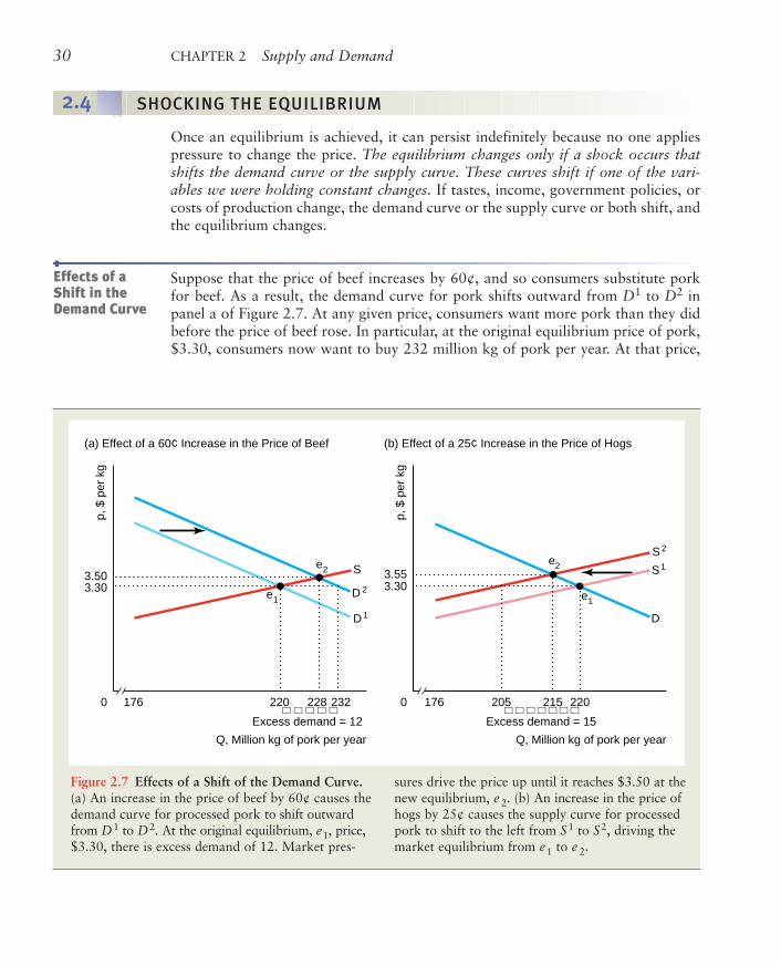
Suppose that the price of beef increases by 60¢, and so consumers substitute porkfor beef. As a result, the demand curve for pork shifts outward from D1 to D2 inpanel a of Figure 2.7. At any given price, consumers want more pork than they didbefore the price of beef rose. In particular, at the original equilibrium price of pork,$3.30, consumers now want to buy 232 million kg of pork per year. At that price,

Effects of aShift in theDemand Curve

Figure 2.7 Effects of a Shift of the Demand Curve.(a) An increase in the price of beef by 60¢ causes thedemand curve for processed pork to shift outwardfrom D1 to D2. At the original equilibrium, e1, price,$3.30, there is excess demand of 12. Market pres-

sures drive the price up until it reaches $3.50 at thenew equilibrium, e 2. (b) An increase in the price ofhogs by 25¢ causes the supply curve for processedpork to shift to the left from S1 to S2, driving themarket equilibrium from e1 to e 2.

D 1

D 2

S1

S2

S

1760 220 228 232


Excess demand = 12


3.303.50

3.303.55

e2

e1 e1

e2

D

p, $

per

kg

p, $

per

kg

(a) Effect of a 60¢ Increase in the Price of Beef (b) Effect of a 25¢ Increase in the Price of Hogs

1760 220205 215

Excess demand = 15

2.4 SHOCKING THE EQUILIBRIUM

Shocking the Equilibrium 31

Effects of aShift in theSupply Curve

however, suppliers still want to sell only 220. As a result, there is excess demand of12. Market pressures drive the price up until it reaches a new equilibrium at $3.50.At that price, firms want to sell 228 and consumers want to buy 228, the new equi-librium quantity. Thus the pork equilibrium goes from e1 to e2 as a result of theincrease in the price of beef. Both the equilibrium price and the equilibrium quan-tity of pork rise as a result of the outward shift of the pork demand curve. Here theincrease in the price of beef causes a shift of the demand curve, causing a movementalong the supply curve.

Now suppose that the price of beef stays constant at its original level but the priceof hogs increases by 25¢. It is now more expensive to produce pork because theprice of a major input, hogs, has increased. As a result, the supply curve for porkshifts to the left from S1 to S2 in panel b of Figure 2.7. At any given price, firms wantto supply less pork than they did before the price of hogs increased. At the originalequilibrium price of pork of $3.30, consumers still want 220, but suppliers are nowwilling to supply only 205, so there is excess demand of 15. Market pressure forcesthe price of pork up until it reaches a new equilibrium at e2, where the equilibriumprice is $3.55 and the equilibrium quantity is 215. The increase in the price of hogscauses the equilibrium price to rise but the equilibrium quantity to fall. Here a shiftof the supply curve results in a movement along the demand curve.

In summary, a change in an underlying factor, such as the price of a substitute orthe price of an input, shifts the demand or supply curve. As a result of this shift inthe demand or supply curve, the equilibrium changes. To describe the effect of thischange in the underlying factor on the market, we compare the original equilibriumprice and quantity to the new equilibrium values.

Mathematically, how does the equilibrium price of pork vary as the price of hogs

changes if the variables that affect demand are held constant at their typical values?

Answer

1. Solve for the equilibrium price of pork in terms of the price of hogs: Thedemand function does not depend on the price of hogs, so we can useEquation 2.3 from before,

Qd = 286 – 20p.

To see how the equilibrium depends on the price of hogs, we use supplyfunction Equation 2.6:

Qs = 178 + 40p – 60ph.

Solved Problem 2.2


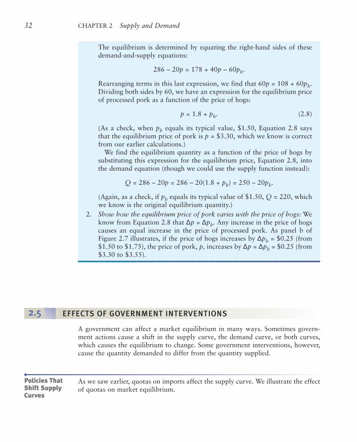
The equilibrium is determined by equating the right-hand sides of thesedemand-and-supply equations:

286 – 20p = 178 + 40p – 60ph.

Rearranging terms in this last expression, we find that 60p = 108 + 60ph.Dividing both sides by 60, we have an expression for the equilibrium priceof processed pork as a function of the price of hogs:

p = 1.8 + ph. (2.8)

(As a check, when ph equals its typical value, $1.50, Equation 2.8 saysthat the equilibrium price of pork is p = $3.30, which we know is correctfrom our earlier calculations.)

We find the equilibrium quantity as a function of the price of hogs bysubstituting this expression for the equilibrium price, Equation 2.8, intothe demand equation (though we could use the supply function instead):

Q = 286 – 20p = 286 – 20(1.8 + ph) = 250 – 20ph.

(Again, as a check, if ph equals its typical value of $1.50, Q = 220, whichwe know is the original equilibrium quantity.)

2. Show how the equilibrium price of pork varies with the price of hogs: Weknow from Equation 2.8 that ∆p = ∆ph. Any increase in the price of hogscauses an equal increase in the price of processed pork. As panel b ofFigure 2.7 illustrates, if the price of hogs increases by ∆ph = $0.25 (from$1.50 to $1.75), the price of pork, p, increases by ∆p = ∆ph = $0.25 (from$3.30 to $3.55).

Policies ThatShift SupplyCurves

A government can affect a market equilibrium in many ways. Sometimes govern-ment actions cause a shift in the supply curve, the demand curve, or both curves,which causes the equilibrium to change. Some government interventions, however,cause the quantity demanded to differ from the quantity supplied.

As we saw earlier, quotas on imports affect the supply curve. We illustrate the effectof quotas on market equilibrium.

2.5 EFFECTS OF GOVERNMENT INTERVENTIONS

Effects of Government Interventions 33

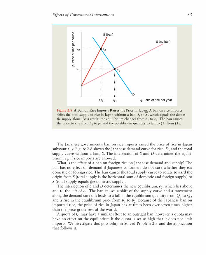
The Japanese government’s ban on rice imports raised the price of rice in Japansubstantially. Figure 2.8 shows the Japanese demand curve for rice, D, and the totalsupply curve without a ban, S. The intersection of S and D determines the equili-brium, e1, if rice imports are allowed.

What is the effect of a ban on foreign rice on Japanese demand and supply? Theban has no effect on demand if Japanese consumers do not care whether they eatdomestic or foreign rice. The ban causes the total supply curve to rotate toward theorigin from S (total supply is the horizontal sum of domestic and foreign supply) toS–

(total supply equals the domestic supply).The intersection of S

–and D determines the new equilibrium, e2, which lies above

and to the left of e1. The ban causes a shift of the supply curve and a movementalong the demand curve. It leads to a fall in the equilibrium quantity from Q1 to Q2and a rise in the equilibrium price from p1 to p2. Because of the Japanese ban onimported rice, the price of rice in Japan has at times been over seven times higherthan the price in the rest of the world.

A quota of Q–

may have a similar effect to an outright ban; however, a quota mayhave no effect on the equilibrium if the quota is set so high that it does not limitimports. We investigate this possibility in Solved Problem 2.3 and the applicationthat follows it.

Figure 2.8 A Ban on Rice Imports Raises the Price in Japan. A ban on rice importsshifts the total supply of rice in Japan without a ban, S, to S

–, which equals the domes-

tic supply alone. As a result, the equilibrium changes from e1 to e 2. The ban causesthe price to rise from p1 to p2 and the equilibrium quantity to fall to Q1 from Q2.

p, P

rice

of r

ice

per

poun

d

Q2 Q1

S (no ban)

D

Q, Tons of rice per year

p2 e2

e1p1

S (ban)–


What is the effect of a United States quota on steel of Q–

on the equilibrium in the

U.S. steel market? Hint: The answer depends on whether the quota binds (is lowenough to affect the equilibrium).

Answer

1. Show how a quota, Q–

, affects the total supply of steel in the United States:The graph reproduces the no-quota total American supply curve of steel,S, and the total supply curve under the quota, S

–(which we derived in

Solved Problem 2.1). At a price below p–, the two supply curves are iden-tical because the quota is not binding: It is greater than the quantity for-eign firms want to supply. Above p–, S

–lies to the left of S.

2. Show the effect of the quota if the original equilibrium quantity is lessthan the quota so that the quota does not bind: Suppose that theAmerican demand is relatively low at any given price so that the demandcurve, Dl, intersects both the supply curves at a price below p–. The equi-libria both before and after the quota is imposed are at e1, where the equi-librium price, p1, is less than p–. Thus if the demand curve lies near enoughto the origin that the quota is not binding, the quota has no effect on theequilibrium.

3. Show the effect of the quota if the quota binds: With a relatively highdemand curve, Dh, the quota affects the equilibrium. The no-quota equi-librium is e2, where Dh intersects the no-quota total supply curve, S. Afterthe quota is imposed, the equilibrium is e3, where Dh intersects the totalsupply curve with the quota, S

–. The quota raises the price of steel in the

United States from p2 to p3 and reduces the quantity from Q2 to Q3.

p, P

rice

of s

teel

per

ton

Q2Q3

Dh (high)

Q1

S (no quota)

Q, Tons of steel per year

p2

p3 e2

e3

e1p1

S (quota)–

p–

Dl (low)

Solved Problem 2.3


AMERICAN STEEL QUOTAS

The U.S. government has repeatedly limited imports of steel into the UnitedStates. In some years, the U.S. government negotiated with the governments ofJapan and several European countries to limit the amount of steel those coun-tries sold in the United States. Various agreements were in effect from 1969through 1974. But the quotas were often set so high that they had no effect.

However, in 1971 and 1972, the quotas were binding for most steel prod-ucts. These quotas raised average U.S. steel prices between 1.2% and 3.5%.

In 1984, President Ronald Reagan announced a new set of voluntary quo-tas, which covered most steel-exporting countries and limited finished steel

imports into the United States to 18.5% of the totalU.S. sales for 1985–1989. These limits on importsdrove up prices. In 1979–1980, in the absence ofquotas, the average U.S. price of steel was approxi-mately the same as the market price in Antwerp,Belgium. In 1984 and 1985, under the Reagan quo-tas, the average U.S. price was about 25% higherthan the corresponding price in Antwerp.

In 1980, pig iron and semifinished steel importsaccounted for only 3.5% of domestic steel use, ashare that remained virtually unchanged through1992. Thereafter, in the absence of quotas, importsrose substantially, and the share of imports reached26.4% by 1998.

In 1999, the U.S. House of Representatives passeda bill calling for a 30% reduction in steel imports;however, the Senate rejected this legislation in the faceof a threatened veto by President Bill Clinton. In2002, President George W. Bush imposed a tariff,which is a tax on imported goods (see Chapter 9), toreduce steel imports. The European Union respondedby threatening retaliatory tariffs on U.S. goods.

Some government policies do more than merely shift the supply or demand curve.For example, governments may control prices directly, a policy that leads to eitherexcess supply or excess demand if the price the government sets differs from theequilibrium price. We illustrate this result with two types of price control programs.When the government sets a price ceiling at p–, the price at which goods are sold maybe no higher than p–. When the government sets a price floor at p

–, the price at which

goods are sold may not fall below p–.

Policies ThatCause Demandto Differ fromSupply

Application

Price Ceilings. Price ceilings have no effect if they are set above the equilibrium pricethat would be observed in the absence of the price controls. If the government saysthat firms may charge no more than p– = $5 per gallon of gas and firms are actuallycharging p = $1, the government’s price control policy is irrelevant. However, if theequilibrium price, p, would be above the price ceiling p–, the price that is actuallyobserved in the market is the price ceiling.

To keep prices from rising in wartime, the United States government has used priceceilings. During World War II, for example, the prices of all staples (such as sugar andgasoline) were controlled. To limit inflation, President Richard Nixon instituted wageand price controls on many goods in 1971–1972. Since 1992, there have been peri-odic debates in Congress about whether to apply price controls to medical services.

The U.S. experience with gasoline illustrates the effects of price controls. In the1970s, the Organization of Petroleum Exporting Countries (OPEC) reduced sup-plies of oil (which is converted into gasoline) to Western countries. As a result, thetotal supply curve for gasoline in the United States—the horizontal sum of domes-tic and OPEC supply curves—shifted to the left from S1 to S2 in Figure 2.9. Becauseof this shift, the equilibrium price of gasoline would have risen substantially, fromp1 to p2. In an attempt to protect consumers by keeping gasoline prices from rising,the U.S. government set price ceilings on gasoline in 1973 and 1979.

The government told gas stations that they could charge no more than p– = p1.Figure 2.9 shows the price ceiling as a solid horizontal line extending from the price


Figure 2.9 Price Ceiling on Gasoline. Supply shifts from S1 to S2. Under the govern-ment’s price control program, gasoline stations may not charge a price above theprice ceiling p– = p1. At that price, producers are willing to supply only Qs, which isless than the amount Q1 = Qd that consumers want to buy. The result is excessivedemand, or a shortage of Qd – Qs.

p, $

per

gal

lon

Qs Q2 Q1 = Qd

Price ceiling

S1

D

S 2

Q, Gallons of gasoline per monthExcess demand

p2

e2

e1

p1 = p–

anim036.html


axis at p–. The price control is binding because p2 > p–. The observed price is the priceceiling. At p–, consumers want to buy Qd = Q1 gallons of gasoline, which is the equi-librium quantity they bought before OPEC acted. However, firms supply only Qsgallons, which is determined by the intersection of the price control line with S2. Asa result of the binding price control, there is excess demand of Qd – Qs.

Were it not for the price controls, market forces would drive up the market priceto p2, where the excess demand would be eliminated. The government price ceilingprevents this adjustment from occurring. As a result, an enforced price ceiling causesa shortage: a persistent excess demand.

At the time of the controls, some government officials argued that the shortageswere caused by OPEC’s cutting off its supply of oil to the United States, but that’snot true. Without the price controls, the new equilibrium would be e2. In this equi-librium, the price, p2, is much higher than before, p1; however, there is no shortage.Moreover, without controls, the quantity sold, Q2, is greater than the quantity soldunder the control program, Qs.

With a binding price ceiling, the supply-and-demand model predicts an equilibriumwith a shortage. In this equilibrium, the quantity demanded does not equal the quan-tity supplied. The reason that we call this situation an equilibrium, even though a short-age exists, is that no consumers or firms want to act differently, given the law. Withoutthe price controls, consumers facing a shortage would try to get more output by offer-ing to pay more, or firms would raise prices. With effective government price controls,they know that they can’t drive up the price, so they live with the shortage.

What happens? Some lucky consumers get to buy Qs units at the low price of p–.Other potential customers are disappointed: They would like to buy at that price,but they cannot find anyone willing to sell gas to them.

What determines which consumers are lucky enough to find goods to buy at thelow price when there are price controls? With enforced price controls, sellers use cri-teria other than price to allocate the scarce commodity. Firms may supply theirfriends, long-term customers, or people of a certain race, gender, age, or religion.They may sell their goods on a first-come, first-served basis. Or they may limiteveryone to only a few gallons.

Another possibility is for firms and customers to evade the price controls. A consumercould go to a gas station owner and say, “Let’s not tell anyone, but I’ll pay you twicethe price the government sets if you’ll sell me as much gas as I want.” If enough cus-tomers and gas station owners behaved that way, no shortage would occur. A studyof 92 major U.S. cities during the 1972 gasoline price controls found no gasolinelines in 52 of them. However, in cities such as Chicago, Hartford, New York,Portland, and Tucson, potential customers waited in line at the pump for an houror more.9 Deacon and Sonstelie (1989) calculated that for every dollar consumerssaved during the 1980 gasoline price controls, they lost $1.16 in waiting time andother factors. This experience may be of importance in Hawaii, where a 2002 lawwill impose gasoline price controls effective in 2004.

9See www.aw.com/perloff, Chapter2, “Gas Lines,” for a discussion of the effects of the 1973 and1979 gasoline price controls.


Price Floors. Governments also commonly use price floors. One of the most impor-tant examples of a price floor is the minimum wage in labor markets.

The minimum wage law forbids employers from paying less than the minimumwage, w. Currently, the U.S. federal minimum wage is $5.15 an hour. Since April1999, Britain has had a national minimum wage, which was £4.20 in October 2002.The minimum wage in the European Union ranges from 1.80€ in Spain to 6.43€ inIreland and to 9.67€ in Luxembourg. If the minimum wage binds—exceeds theequilibrium wage, w*—the minimum wage creates unemployment, which is a per-sistent excess supply of labor.10

10Where the minimum wage applies to only a few labor markets (Chapter 10) or where only asingle firm hires all the workers in a market (Chapter 15), a minimum wage may not causeunemployment (see Card and Krueger, 1995, for empirical evidence). The U.S. Department ofLabor maintains at its Web site (www.dol.gov) an extensive history of the minimum wage law,labor markets, state minimum wage laws, and other information.

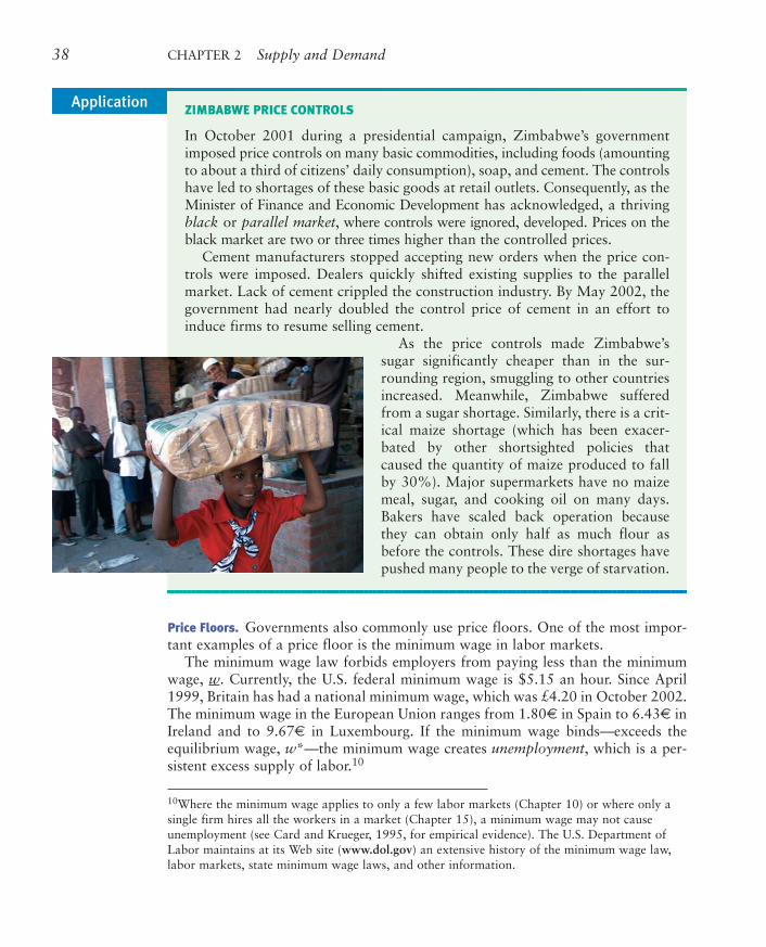
ZIMBABWE PRICE CONTROLS

In October 2001 during a presidential campaign, Zimbabwe’s governmentimposed price controls on many basic commodities, including foods (amountingto about a third of citizens’ daily consumption), soap, and cement. The controlshave led to shortages of these basic goods at retail outlets. Consequently, as theMinister of Finance and Economic Development has acknowledged, a thrivingblack or parallel market, where controls were ignored, developed. Prices on theblack market are two or three times higher than the controlled prices.

Cement manufacturers stopped accepting new orders when the price con-trols were imposed. Dealers quickly shifted existing supplies to the parallelmarket. Lack of cement crippled the construction industry. By May 2002, thegovernment had nearly doubled the control price of cement in an effort toinduce firms to resume selling cement.

As the price controls made Zimbabwe’ssugar significantly cheaper than in the sur-rounding region, smuggling to other countriesincreased. Meanwhile, Zimbabwe sufferedfrom a sugar shortage. Similarly, there is a crit-ical maize shortage (which has been exacer-bated by other shortsighted policies thatcaused the quantity of maize produced to fallby 30%). Major supermarkets have no maizemeal, sugar, and cooking oil on many days.Bakers have scaled back operation becausethey can obtain only half as much flour asbefore the controls. These dire shortages havepushed many people to the verge of starvation.

Application


11The minimum wage could raise the wage enough that total wage payments, wL, rise despite thefall in demand for labor services. If the workers could share the unemployment—everybody worksfewer hours than he or she wants—all workers could benefit from the minimum wage.

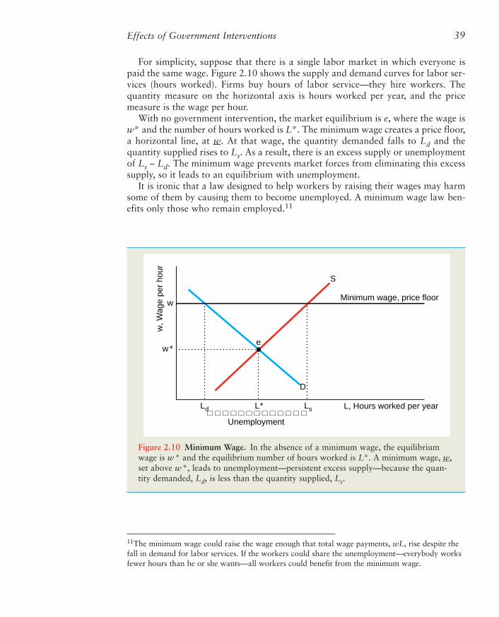
Figure 2.10 Minimum Wage. In the absence of a minimum wage, the equilibriumwage is w * and the equilibrium number of hours worked is L*. A minimum wage, w,set above w *, leads to unemployment—persistent excess supply—because the quan-tity demanded, Ld, is less than the quantity supplied, Ls.

w, W

age

per

hour

Ld L* Ls

Minimum wage, price floor

S

D

L, Hours worked per year

Unemployment

ew *

w

For simplicity, suppose that there is a single labor market in which everyone ispaid the same wage. Figure 2.10 shows the supply and demand curves for labor ser-vices (hours worked). Firms buy hours of labor service—they hire workers. Thequantity measure on the horizontal axis is hours worked per year, and the pricemeasure is the wage per hour.

With no government intervention, the market equilibrium is e, where the wage isw* and the number of hours worked is L*. The minimum wage creates a price floor,a horizontal line, at w. At that wage, the quantity demanded falls to Ld and thequantity supplied rises to Ls. As a result, there is an excess supply or unemploymentof Ls – Ld. The minimum wage prevents market forces from eliminating this excesssupply, so it leads to an equilibrium with unemployment.

It is ironic that a law designed to help workers by raising their wages may harmsome of them by causing them to become unemployed. A minimum wage law ben-efits only those who remain employed.11


Why SupplyNeed NotEqual Demand

The price ceiling and price floor examples show that the quantity supplied does notnecessarily equal the quantity demanded in a supply-and-demand model. The quan-tity supplied need not equal the quantity demanded because of the way we definedthese two concepts. We defined the quantity supplied as the amount firms want tosell at a given price, holding other factors that affect supply, such as the price ofinputs, constant. The quantity demanded is the quantity that consumers want to buyat a given price, if other factors that affect demand are held constant. The quantity

MINIMUM WAGE LAW IN PUERTO RICO

In 1938, the Fair Labor Standards Act established a w = 25¢ per hour mini-mum wage for many U.S. industries engaged in interstate commerce. This ratewas at or below the equilibrium wage in most of these industries, so this pricefloor had little effect. Unfortunately, the same minimum wage was applied toPuerto Rico, a self-governing island commonwealth in free association withthe United States, whose residents are U.S. citizens. Puerto Rico’s averagewage was much lower: only about 7¢ (= w* in Figure 2.10) in tobacco andcoffee industries, 12¢ in fruit canning, 14¢ in laundries, and 18¢ in apparelindustries.

Employers in several important Puerto Rican industries screamed bloodymurder. Employers in the tobacco-stemming industry would not comply withthe law and practically locked out workers, making them unemployed.

The needlework export industries were decimated. A comparison of1939–1940 to 1940–1941 shows that exports fell by 61% in cotton manufac-turing and linen manufacturing, 71% in silk manufacturing, and 47% in otherneedlework manufacturing.

This loss of jobs and output devastated Puerto Rico. In response, the U.S.Congress established special minimum wages for specific Puerto Ricanindustries. For example, by the end of 1940, the rate fell to as low as 12.5¢in some parts of the needlework industry. Starting in 1974, the Puerto Ricanminimum wage was raised gradually to the U.S. level. By 1983, both mini-mums were the same, $3.35. Even today, Puerto Rico has some industrieswith lower rates.

In 2002, the minimum wage was half of the average hourly earnings inmanufacturing in Puerto Rico but only about one-third (34%) on the main-land. Castillo-Freeman and Freeman (1992) estimate that island employmentwould have been 8% to 10% higher in 1987 if the minimum wage had beenset so that the ratio of the minimum to the average wage was comparable tothat in the United States. They find that the change in the minimum wagewas responsible for one-third of the drop in the employment rate (the ratioof employment to population) in Puerto Rico from 1975 to 1987.

Application

When to Use the Supply-and-Demand Model 41

that firms want to sell and the quantity that consumers want to buy at a given priceneed not equal the actual quantity that is bought and sold.

When the government imposes a binding price ceiling of p– on gasoline, the quan-tity demanded is greater than the quantity supplied. Despite the lack of equalitybetween the quantity supplied and the quantity demanded, the supply-and-demandmodel is useful in analyzing this market because it predicts the excess demand thatis actually observed.

We could have defined the quantity supplied and the quantity demanded so thatthey must be equal. If we were to define the quantity supplied as the amount firmsactually sell at a given price and the quantity demanded as the amount consumersactually buy, supply must equal demand in all markets because the quantitydemanded and the quantity supplied are defined to be the same quantity.

It is worth pointing out this distinction because many people, including politiciansand newspaper reporters, are confused on this point. Someone insisting that “demandmust equal supply” must be defining demand and supply as the actual quantities sold.

Because we define the quantities supplied and demanded in terms of people’swants and not actual quantities bought and sold, the statement that “supply equalsdemand” is a theory, not merely a definition. This theory says that the equilibriumprice and quantity in a market are determined by the intersection of the supply curveand the demand curve if the government does not intervene. Further, we use themodel to predict excess demand or excess supply when a government does controlprice. The observed gasoline shortages during the period when the U.S. governmentcontrolled gasoline prices are consistent with this prediction.

As we’ve seen, supply-and-demand theory can help us to understand and predictreal-world events in many markets. Through Chapter 10, we discuss competitivemarkets in which the supply-and-demand model is a powerful tool for predictingwhat will happen to market equilibrium if underlying conditions—tastes, incomes,and prices of inputs—change. The types of markets for which the supply-and-demand model is useful are described at length in these chapters, particularlyChapter 8. Briefly, this model is applicable in markets in which:

■ Everyone is a price taker: Because no consumer or firm is a very large part of themarket, no one can affect the market price. Easy entry of firms into the market,which leads to a large number of firms, is usually necessary to ensure that firmsare price takers.

■ Firms sell identical products: Consumers do not prefer one firm’s good toanother.

■ Everyone has full information about the price and quality of goods: Consumersknow if a firm is charging a price higher than the price others set, and theyknow if a firm tries to sell them inferior-quality goods.

2.6 WHEN TO USE THE SUPPLY-AND-DEMAND MODEL


■ Costs of trading are low: It is not time consuming, difficult, or expensive fora buyer to find a seller and make a trade or for a seller to find and trade witha buyer.

Markets with these properties are called perfectly competitive markets. Where there are many firms and consumers, no single firm or consumer is a large

enough part of the market to affect the price. If you stop buying bread or if one ofthe many thousands of wheat farmers stops selling the wheat used to make thebread, the price of bread will not change. Consumers and firms are price takers:They cannot affect the market price.

In contrast, if there is only one seller of a good or service—a monopoly (seeChapter 11)—that seller is a price setter and can affect the market price. Becausedemand curves slope downward, a monopoly can increase the price it receives byreducing the amount of a good it supplies. Firms are also price setters in anoligopoly—a market with only a small number of firms—or in markets where theysell differentiated products so that a consumer prefers one product to another (seeChapter 13). In markets with price setters, the market price is usually higher than thatpredicted by the supply-and-demand model. That doesn’t make the model generallywrong. It means only that the supply-and-demand model does not apply to marketswith a small number of sellers or buyers. In such markets, we use other models.

If consumers have less information than a firm, the firm can take advantage ofconsumers by selling them inferior-quality goods or by charging a much higher pricethan that charged by other firms. In such a market, the observed price is usuallyhigher than that predicted by the supply-and-demand model, the market may notexist at all (consumers and firms cannot reach agreements), or different firms maycharge different prices for the same good (see Chapter 19).

The supply-and-demand model is also not entirely appropriate in markets inwhich it is costly to trade with others because the cost of a buyer’s finding a selleror of a seller’s finding a buyer are high. Transaction costs are the expenses of find-ing a trading partner and making a trade for a good or service other than the pricepaid for that good or service. These costs include the time and money spent to findsomeone with whom to trade. For example, you may have to pay to place a news-paper advertisement to sell your gray 1990 Honda with 137,000 miles on it. Or youmay have to go to many stores to find one that sells a shirt in exactly the color youwant, so your transaction costs includes transportation costs and your time. Thecost of a long-distance call to place an order is a transaction cost. Other transactioncosts include the costs of writing and enforcing a contract, such as the cost oflawyers’ time. Where transaction costs are high, no trades may occur, or if they dooccur, individual trades may occur at a variety of prices (see Chapters 12 and 19).

Thus the supply-and-demand model is not appropriate in markets in which thereare only one or a few sellers (such as electricity), firms produce differentiated prod-ucts (music CDs), consumers know less than sellers about quality or price (usedcars), or there are high transaction costs (nuclear turbine engines). Markets in whichthe supply-and-demand model has proved useful include agriculture, finance, labor,construction, services, wholesale, and retail.

Questions 43

1. Demand: The quantity of a good or servicedemanded by consumers depends on their tastes,the price of a good, the price of goods that are sub-stitutes and complements, their income, informa-tion, government regulations, and other factors.The Law of Demand—which is based on observa-tion—says that demand curves slope downward.The higher the price, the less of the good isdemanded, holding constant other factors thataffect demand. A change in price causes a move-ment along the demand curve. A change inincome, tastes, or another factor that affectsdemand other than price causes a shift of thedemand curve. To get a total demand curve, wehorizontally sum the demand curves of individualsor types of consumers or countries. That is, weadd the quantities demanded by each individual ata given price to get the total demanded.

2. Supply: The quantity of a good or service suppliedby firms depends on the price, costs, governmentregulations, and other factors. The market supplycurve need not slope upward but usually does. Achange in price causes a movement along the sup-ply curve. A change in the price of an input orgovernment regulation causes a shift of the supplycurve. The total supply curve is the horizontalsum of the supply curves for individual firms.

3. Market equilibrium: The intersection of thedemand curve and the supply curve determines theequilibrium price and quantity in a market.Market forces—actions of consumers and firms—

drive the price and quantity to the equilibriumlevels if they are initially too low or too high.

4. Shocking the equilibrium: A change in an under-lying factor other than price causes a shift of thesupply curve or the demand curve, which altersthe equilibrium. For example, if the price of beefrises, the demand curve for pork shifts outward,causing a movement along the supply curve andleading to a new equilibrium at a higher priceand quantity. If changes in these underlying fac-tors follow one after the other, a market thatadjusts slowly may stay out of equilibrium for anextended period.

5. Effects of government interventions: Some govern-ment policies—such as a ban on imports—cause ashift in the supply or demand curves, thereby alter-ing the equilibrium. Other government policies—such as price controls or a minimum wage—causethe quantity supplied to be greater or less than thequantity demanded, leading to persistent excessesor shortages.

6. When to use the supply-and-demand model: Thesupply-and-demand model is a powerful tool toexplain what happens in a market or to make pre-dictions about what will happen if an underlyingfactor in a market changes. This model, however,is applicable only in markets with many buyersand sellers; identical goods; certainty and fullinformation about price, quantity, quality,incomes, costs, and other market characteristics;and low transaction costs.

Summary

Questions

If you ask me anything I don’t know, I’m not going to answer. —Yogi Berra

Answers to selected questions and problems appear at the back of the book.

1. In December 2000, Japan reported that test ship-ments of U.S. corn had detected StarLink, a geneti-cally modified corn that is not approved for humanconsumption in the United States. As a result, Japan

and some other nations banned U.S. imports. Use agraph to illustrate why this ban, which caused U.S.corn exports to fall 4%, resulted in the price of cornfalling 11.1% in the United States in 2001–2002.

QUIZ

Q A

gloss_fc_043.html

ques_fc_043.html

quiz012.html


2. Increasingly, instead of advertising in newspapers,individuals and firms use Web sites that offer freeclassified ads, such as Realtor.com, Jobs.com,Monster.com, and portals like Yahoo and AmericaOnline. Using a supply-and-demand model,explain what will happen to the equilibrium levelsof newspaper advertising as the use of the Internetgrows. Will the growth of the Internet affect thesupply curve, the demand curve, or both? Why?

3. In 2002, the U.S. Fish and Wildlife Service pro-posed banning imports of beluga caviar to protectthe beluga sturgeon in the Caspian and Black seas,whose sturgeon population has fallen 90% in thelast two decades. The United States imports 80%of the world’s beluga caviar. On the world’s legalwholesale market, a kilogram of caviar costs anaverage of $500, and about $100 million worth issold per year. What effect would the U.S. ban haveon world prices and quantities? Would such a banhelp protect the beluga sturgeon?

4. The U.S. supply of frozen orange juice comes fromFlorida and Brazil. What is the effect of a freezethat damages oranges in Florida on the price offrozen orange juice in the United States and on thequantities of orange juice sold by Floridian andBrazilian firms?

5. What is the effect of a quota Q–

> 0 on equilibriumprice and quantity? (Hint: Carefully show how thetotal supply curve changes.)

6. Usury laws place a ceiling on interest rates thatlenders such as banks can charge borrowers. Low-income households in states with usury laws havesignificantly lower levels of consumer credit(loans) than comparable households in stateswithout usury laws (Villegas, 1989). Why? (Hint:The interest rate is the price of a loan, and theamount of the loan is the quantity measure.)

7. In 1999, after nearly 20 years of rent control inBerkeley, California, the elimination of the law ledto an estimated rise in rents of nearly 40%. Usingsupply-and-demand models, illustrate how the lawand then its elimination affected the rental housing

market. Discuss the effects on the equilibriumrental price and the quantity of housing rented.

8. After a major earthquake struck Los Angeles inJanuary 1994, several stores raised the price ofmilk to over $6 a gallon. The local authoritiesannounced that they would investigate and thatthey would enforce a law prohibiting priceincreases of more than 10% during an emergencyperiod. What is the likely effect of such a law?

9. Is it possible that an outright ban on foreignimports will have no effect on the equilibriumprice? (Hint: Suppose that imports occur only atrelatively high prices.)

10. If certain jurisdictions ban the use of skateboardson city streets, what is the likely effect on the mar-ket for skateboards? How do such laws affect thesupply curve, the demand curve, and equilibriumprice and quantity?

11. The New York Times reported in 1997 that a crack-down on a cocaine-smuggling ring caused cocaineprices in Manhattan to rise from $20,000 to$30,000 a kilogram. Illustrate in a supply-and-demand diagram why this happened, and explainin words.

12. In 1996, a group of American doctors called for alimit on the number of foreign-trained physicianspermitted to practice in the United States. Whateffect would such a limit have on the equilibriumquantity and price of doctor services in the UnitedStates? How are American-trained doctors andconsumers affected?

13. Suppose that cotton is produced only in the UnitedStates and China. The U.S. government says that ifan American farmer sells a bale of cotton at theworld price, p, the government will give the farmer(p* – p) per bale, where p* > p. What happens tothe quantities sold by American and Chinesegrowers and the world price of cotton?

14. Use a supply-and-demand diagram to explain thestatement “Talk is cheap because supply exceedsdemand.” At what price is this comparison beingmade?

Problems 45

15. Using the estimated demand function for pro-cessed pork in Canada (Equation 2.2), determinehow price changes as the quantity demandedincreases by one unit (that is, the quantitydemanded increases by 1 million kg per year).(Hint: Rewrite the demand function so that priceis a function of quantity.)

16. Using the estimated demand function for pro-cessed pork in Canada (Equation 2.2), show howthe quantity demanded at a given price changes asper capita income, Y, increases by $100 a year.

17. Suppose that the price of beef, pb, in Canadaincreased by 30%, from $4 to $5.20. How doesthe demand curve for processed pork shift?

18. If the supply of corn by the United States is Qa =a + bp, and the supply by the rest of the world isQr = c + ep, what is the world supply?

19. The demand function for a good is Q = a – bp, and

the supply function is Q = c + ep, where a, b, c, ande are positive constants. Solve for the equilibriumprice and quantity in terms of these four constants.

20. Show how the equilibrium quantity of pork varieswith income.

21. Using the equations for processed pork demand(Equation 2.2) and supply (Equation 2.6), solvefor the equilibrium price and quantity in terms ofthe price of hogs, ph; the price of beef, pb; the priceof chicken, pc; and income, y. If ph = 1.5 (dollarsper kg), pb = 4 (dollars per kg), pc = 31

3 (dollars perkg), and y = 12.5 (thousands dollars), what are theequilibrium price and quantity?

22. The demand function for roses is Q = a – bp, andthe supply function is Q = c + ep + ft, where a, b,c, e, and f are positive constants and t is the aver-age temperature in a month. Show how the equi-librium quantity and price vary with temperature.

Problems

ch02 perloff 16073 - wps.aw.comwps.aw.com/wps/media/objects/591/605493/protected/ch02/ch02.pdf ·...

Documents