cha jobs econ dev 2011

8/12/2019 CHA Jobs Econ Dev 2011

http://slidepdf.com/reader/full/cha-jobs-econ-dev-2011 1/39

JOB CREATION AND ECONOMIC

DEVELOPMENT OPPORTUNITIES

IN THE CANADIAN HYDROPOWER

MARKET

R ACHEL DESROCHERS

ISABELLE MONTOUR

ANNIE GRÉGOIRE

JÉRÔME CHOTEAU

E RWAN TURMEL

SEPTEMBER 26, 2011



J O B C R E A T I O N A N D E C O N O M I C D E V E L O P M E N T O P P O R T U N I T I E S I N T H E C A N A D I A N H Y D R O P O W E R M A R K E T

E X E C U T I V E S U M M A R Y

The Canadian Hydropower Association (CHA) requested a team of MBA students from HEC

Montreal to research hydroelectricity projects that will be happening over the next 20 years in

order to estimate the jobs and Gross Domestic Product (GDP) value that these projects would

create.

The HEC team conducted the study from July 4th through August 5th, 2011. Three scenarios related

to different levels of hydropower deployment in each province and territory were developed and

named: “Business as Usual”, “Mid-scenario” and “Optimistic” scenario. The information about

hydropower projects planned for the next 20 years was gathered from CHA members and a few

other industry players who were available during the period of the study. If needed, public

information was utilized to complete the gaps, as well as estimates obtained from correlation with

available data.

The Canadian IO Model developed by Statistics Canada was used to measure the impacts of the

Canadian hydropower projects on job creation and GDP. This IO Model, like any input-output

model, illustrates macroeconomic relationships between suppliers and producers, within an

economy, at a regional or national level. Two different shocks were created in the 2007 IO Model

in order to get both construction and operating benefits.

A total of 158 hydropower projects for the next 20 years were identified (non-small hydro projects

only) within three regions (Western region (composed of Yukon, British Colombia & Alberta),

Central region (Northern Territories, Nunavut, Saskatchewan & Manitoba) and Eastern region

(Ontario, Quebec and Atlantic Canada). The data indicate that the projects are split almost equally

between the Western and the Eastern regions of Canada. About a third of the projects are

upgrades or restorations mainly located in Eastern Canada. More than 80% of new constructions

are run-of-rivers (mostly concentrated in the Western region) while most storage hydro projectsare located in the Eastern region. In the most optimistic case, Canada could foresee the

installation of 29,060 MW of capacity which represents an investment in construction of

$127.7 billion (in 2011 dollars). The operation of all these new facilities would represent additional

revenues of $172.4 billion for generators. Based on the collected data, the Canadian hydropower

output would increase by 137 TWh in the coming 20 years in the “Optimistic” scenario.

The construction of hydropower projects would create up to 1,036,564 jobs which is equivalent to

51,828 full-time jobs that would last for twenty years. This would represent 0.3% of the 2010

Canadian workforce. In the “Optimistic” scenario, this would also increase the yearly Canadian

GDP by 0.38% and could represent up to 45% of the global estimated investment in the electricity

sector required by 2030. This study, unlike past studies, collected project information directly from

Canadian hydropower generators. It is also important to note that this study is considering direct,

indirect and induced jobs when comparing to other studies (like Navigant 2007 or Wires and the

Brattle Group 2011). The limitations related to the use of the IO Models should also be considered

when using the results.




T A B L E O F C O N T E N T S

E X E C U T I V E S U M M A R Y . . . . . . . . . . . . . . .. . . . . . . . . . . . . . . . .. . . . . . . . . . . . . . . . .. . . . . . . . . . . . . . . . .. . . . . . . . . . .P A G E 1

T A B L E O F C O N T E N T S . . . . . . . . . . . . . . . . .. . . . . . . . . . . . . . . . .. . . . . . . . . . . . . . . . .. . . . . . . . . . . . . . . . .. . . . . . . . . . .P A G E 2

I N T R O D U C T I O N . . . . . . . . . . . . . . .. . . . . . . . . . . . . . . .. . . . . . . . . . . . . . . . .. . . . . . . . . . . . . . . . . .. . . . . . . . . . . . . . . . .. . . . .P A G E 3 T R E N D S A N D P R E S E N T H Y D R O S I T U A T I O N I N C A N A D A . . . . . . . . . . . . . . . .. . . . . . . . P A G E 4

P R O J E C T M E T H O D O L O G Y . . . . . . . . . . . . . . . .. . . . . . . . . . . . . . . . . .. . . . . . . . . . . . . . . . .. . . . . . . . . . . . . . . . .. . . . .P A G E 6 DA T A G A T H E R I N G . . . . . . . . . . . . . . . . . . . . . . . . . . . . . . . . . . . . . . . . . . . . . . . . . . . . . . . . . . . . . . . . . . .. . . . . . . . . . . . . . . . . . . . . . . . . . . . . . . . P A G E 6 P U B L I C I N F O R M A T I O N . . . . . . . . . . . . . . . . . . . . . . . . . . . . . . . . . . . . . . . . . . . . . . . . . . . . . . . .. . . . . . . . . . . . . . . . . . . . . . . . . . . . . . . . . . . . . . . . . P A G E 7 I N T E R V I E W S . . . . . . . . . . . . . . . . . . . . . . . . . . . . . . . . . . .. . . . . . . . . . . . . . . . . . . . . . . . . . . . . . . . . . . . . . . . . . . . . . . . . .. . . . . . . . . . . . . . . . . . . . . . . . P A G E 7 DA T A A N A L Y S I S . . . . . . . . . . . . . . . . . . . . . . . . . . . . . . . . . . . . . . . . . . . . . . .. . . . . . . . . . . . . . . . . . . . . . . . . . . . . . . . . . . . . . . . . . . . . . . . . . .. . . . . . P A G E 8 I N P U T -OU T P U T M O D E L O F S T A T I S T I C S CA N A D A . . . . . . . . . . . . . . . . . . . . . . . . . . . . . . . . . . . . . . . . . . . . . . . . . . . . . . . . . . .. . . . . . . . P A G E 8 SC E N A R I O S . . . . . . . . . . . . . . . . . . . . . . . . . . . . . . . . . . . . . . . . . . . .. . . . . . . . . . . . . . . . . . . . . . . . . . . . . . . . . . . . . . . . . . . . . . . . . .. . . . . . . . . . . . . . . PA G E 10 CO N S T R U C T I O N C O S T E S T I M A T I O N . . . . . . . . . . . . . . . . . . . . . . . . . . . . . . . . . . . . . . . . . . . . . . . . . .. . . . . . . . . . . . . . . . . . . . . . . . . . . . . . . PA G E 11 OP E R A T I N G R E V E N U E S E S T I M A T I O N - E L E C T R I C I T Y P R I C E S . . . . . . . . . . . . . . . . . . . . . . . . . . . . . . . . . . . . . . . . . . . . . . . . . . . . . . P A G E 11

CA S H FL O W S C A L C U L A T I O N S & AS S U M P T I O N S . . . . . . . . . . . . . . . . . . . . . . . . . . . . . . . . . . . . . . . . . . . . .. . . . . . . . . . . . . . . . . . . . . . . PA G E 12 DA T A AG G R E G A T I O N . . . . . . . . . . . . . . . . . . . . . . . . . . . . . . . . . . . . . . . . . . . . . . . . .. . . . . . . . . . . . . . . . . . . . . . . . . . . . . . . . . . . . . . . . . . . . . . . . PA G E 13

C O L L E C T E D D A T A . . . . . . . . . . . . . . . . .. . . . . . . . . . . . . . . . .. . . . . . . . . . . . . . . . .. . . . . . . . . . . . . . . . .. . . . . . . . . . . . . . .P A G E 1 4 P R O J E C T E D I N S T A L L E D CA P A C I T Y . . . . . . . . . . . . . . . . . . . . . . . . . . . . . . . . . . . . . . . . . . . .. . . . . . . . . . . . . . . . . . . . . . . . . . . . . . . . . . . . . . . PA G E 15 CO N S T R U C T I O N CA S H F L O W S . . . . . . . . . . . . . . . . . . . . . . . . . . . . . . . . . . . . . . . . . . . . . . . . . . . . . . . . . . . . . . . . . . . . . . . . . . . . . . . . . . . . . . . . PA G E 16 OP E R A T I O N R E V E N U E S . . . . . . . . . . . . . . . . . . . . . . . . . . . . . . . . . . . . . . . . . . . . . . .. . . . . . . . . . . . . . . . . . . . . . . . . . . . . . . . . . . . . . . . . . . . . . . . PA G E 18 ME A N A N N U A L O U T P U T . . . . . . . . . . . . . . . . . . . . . . . . . . . . . . . . . . . . . . . . . . . . . .. . . . . . . . . . . . . . . . . . . . . . . . . . . . . . . . . . . . . . . . . . . . . . . . PA G E 19

R E S U L T S . . . . . . . . . . . . . . .. . . . . . . . . . . . . . . . .. . . . . . . . . . . . . . . . .. . . . . . . . . . . . . . . . .. . . . . . . . . . . . . . . . .. . . . . . . . . . . . . . .P A G E 2 1 P R O J E C T E D F U L L T I M E E Q U I V A L E N T J OB S . . . . . . . . . . . . . . . . . . . . . . . . . . . . . . . . . . . . . . . . . .. . . . . . . . . . . . . . . . . . . . . . . . . . . . . . . PA G E 21 GR O S S D O M E S T I C PR O D U C T . . . . . . . . . . . . . . . . . . . . . . . . . . . . . . . . . . . . . . . . . . . . . . . . . .. . . . . . . . . . . . . . . . . . . . . . . . . . . . . . . . . . . . . . . PA G E 24

C O N C L U S I O N . . . . . . . . . . . . . . .. . . . . . . . . . . . . . . . . .. . . . . . . . . . . . . . . . .. . . . . . . . . . . . . . . . .. . . . . . . . . . . . . . . . .. . . . . .P A G E 2 7 L I S T O F F I G U R E S . . . . . . . . . . . . . . .. . . . . . . . . . . . . . . . .. . . . . . . . . . . . . . . . .. . . . . . . . . . . . . . . . . .. . . . . . . . . . . . . . . ..P A G E 2 9

G L O S S A R Y . . . . . . . . . . . . . . . . .. . . . . . . . . . . . . . . . . .. . . . . . . . . . . . . . . . .. . . . . . . . . . . . . . . . .. . . . . . . . . . . . . . . . .. . . . . . . . .P A G E 3 0

R E F E R E N C E S . . . . . . . . . . . . . . . .. . . . . . . . . . . . . . . . . .. . . . . . . . . . . . . . . . .. . . . . . . . . . . . . . . . .. . . . . . . . . . . . . . . . .. . . . . .P A G E 3 1

A P P E N D I X A – I N T E R V I E W E D O R G A N I Z A T I O N S . . . . . . . . . . . . . . . .. . . . . . . . . . . . . . . . .. . . P A G E 3 3

A P P E N D I X B – I N P U T - O U T P U T M O D E L L I M I T A T I O N S . . . . . . . . . . . . . . .. . . . . . . . . . . . P A G E 3 4

A P P E N D I X C – E L E C T R I C I T Y P R I C E S P R O J E C T I O N S . . . . . . . . . . . . . . . .. . . . . . . . . . . . . . . P A G E 3 7




I N T R O D U C T I O N

Hydroelectricity is the best known form of renewable energy. It has been used for approximately

to 130 years. Canada is the second largest hydropower producer in the world after China. A strong

Canadian hydroelectricity industry not only ensures a renewable energy supply for Canadians, but

provides many other benefits such as regional development, greenhouse gas (GHG) emission

reduction, fostering Canadian engineering capabilities and providing Canadian companies a great

position in energy markets. Investment in hydropower also supports employment and stimulates

the economy. Despite a decrease in spending since the 1970s, the last decade has seen a slow

increase in new capacity investment as reliability needs are getting addressed and aging facilities

are being upgraded or replaced.

The Canadian Hydropower Association (CHA) selected a team of MBA students from HEC Montreal

to research hydroelectricity projects that will be happening over the next 20 years and to estimate

their economic impacts. More specifically, this study is focused on the jobs and Gross Domestic

Product (GDP) value that will be created by additional hydropower deployment. To measure the

employment and overall economic activity during the construction and operation phases, the 2007input-output model from Statistics Canada was used. These kinds of models are universally used

by economists and policy analysts to estimate how specific investments affect the different sectors

of a provincial or national economy. The purpose of this report is to present the results of the

study and to highlight the facts of interest.

This mandate was conducted as part of the MBA supervised consulting field project. The team was

supervised by Olivier Bahn, Associate Professor at the Department of Management Sciences at

HEC Montreal.




Hydro63.10%

Fossil

Fuel21.60%

Nuclear15.00%

Wind0.30%

T R E N D S A N D P R E S E N T H Y D R O S I T U A T I O N I N C A N A

By definition, hydropower captures the energy released from falling or flowing water. The kinetic

energy produced is first converted into mechanical energy and then into electricity. Small

hydropower developments were common in North America until the 1940s and the transition to

large hydro projects occurred between 1940 and 1970. Hydropower plants can be classified in

terms of their size, operating head, application and the way they are operated. There are two

main types of conventional hydropower installations in Canada: reservoir and run-of-river. The

reservoir produces electricity by using the water accumulated in a large reservoir. The run-of-river

uses mainly natural flow and a small headpond. Both hydropower installations are very similar,

except on the volume of the live storage. By definition, the run-of-river projects will hold several

hours of water inflow; the live reservoir will hold up to several months’ storage (RTA, 2010).

Canada is one of the world's largest producers of

hydroelectricity. In 2009, Canada generated a total of

575.2 TWh and consumed 548.8 TWh (CEA, 2009).

63.1% of this electricity is produced from hydropower

(Statistics Canada, 2011b).

Figure 2 – Canadian Electricity Generation, 1990-2009

(Natural Resources Canada, 2011)

Figure 1 – Electricity

Generation in Canada bysources (Statistics Canada,

2011b)




The electricity networks of Canada and the United States are highly integrated and the vast

potential for hydropower generation in Canada and demands for more clean energy in the U.S. will

reinforce this integration. Also, the introduction of Canadian legislation to significantly reduce

emissions from coal-fired plants will advantage the hydropower industry. Other factors like

anticipated restrictions on carbon emissions and the growth of the United States’ demand creates

a big market for Canada's hydropower resources. Several deals to export power to the U.S. have

already been made (ex: in Minnesota, Vermont and New England) and more are looming.

An estimated 475 hydroelectric plants with a capacity of more than 72,000 MW are currently

operating in Canada (Centre for Energy, 2011). According to an EEM study (EEM, 2006)

commissioned by the CHA, "Canada has 163,000 MW of untapped hydropower potential", which

includes 5,500 sites of small hydro potential (sites with less than 10 MW of capacity).

Figure 3 – Canadian Hydropower Plant (Centre for Energy, 2011)




P R O J E C T M E T H O D O L O G Y

The HEC team conducted the study from July 4th through August 5th, 2011. The following tasks

were completed during the project:

• Questionnaire design based on required data;

•

Extensive research of public data related to Canadian hydropower projects;

• Information gathering about additional hydropower projects planned for the next 20 years

from CHA members and a few other industry players who were available during the period of

the study;

• Development of three scenarios related to different levels of development based on the

amount of support for additional hydropower deployment in each province and territory;

• Projection of direct, indirect and induced job creation related to these scenarios;

• Projection of Gross Domestic Product (GDP) increase related to these scenarios;

•

Aggregation of data and results; and,

• Results analysis and report preparation.

Specific methodologies developed in order to complete main tasks are presented hereafter.

DATA G A T H E R I N G

The objective of the data gathering was to collect information on potential hydropower projects

that could take place in the coming 20 years. The main source of information was CHA members

who have been interviewed based on the questionnaire designed earlier.

All projects that have been evaluated in the market were considered, including those noteconomically feasible in the past, assuming that they may become feasible in the near future.

Projects include new constructions and major upgrades. The following data were gathered when

available for each potential project:

• Type of project (run-of-river, reservoir, turbine replacement, dam upgrades/restorations, etc.);

•

Likelihood that the project will happen;

• Year at which this project will begin;

• Year at which the major proportion of the budget will be spent;

•

Construction/restoration duration;

• Expected date of commissioning;

•

Estimated cost of the project (if available, costs on a year-by-year basis);

• Additional capacity installed;

• Portion of the production planned for exportation;




All Canadian hydro-generators

have been contacted

•

Estimated mean annual output;

• Estimated revenues related to the added capacity; and,

• Owners of the project.

Experts from consulting and engineering firms were consulted to confirm certain data. When this

was impossible, data were estimated based on available information (see Data Analysis).

P U B L I C I N F O R M A T I O N

An extensive review of all the hydro projects happening in each province and territory was done

based on public information available on the Internet. This allowed a general understanding of the

hydroelectricity market in Canada and a more specific understanding of the current projects. A list

was created with all projects presented in reliable documents, i.e. those produced by either

hydropower generators, provincial utilities or governments. General information available on

these projects was gathered. This list was also useful in identifying major Canadian players in the

industry. It should be noted that the objective was not to evaluate the overall Canadian

hydroelectricity potential but only active projects.

Data related to projects smaller than 10 MW (“small projects” according to the Canadian

Electricity Association definition) were not gathered using interviews. Rather, a specific amount of

small hydro was assigned to each province based on the estimation of the Canadian potential for

small hydro. This way, 5,000 MW among a global potential of 15,000 MW have been allocated to

different provinces and territories using current potential distribution and expert judgment

(EIA, 2010).

The data gathered from CHA and non-CHA members were used to correct and to complete the

public project list, as presented in Appendix A.

I N T E R V I E W S

The data collection phase of the study took place from July 4 th to 22nd, 2011. CHA members were

contacted to collect both technical and economic hydropower potential information. Membership

of the CHA spans the breadth of the industry and includes hydropower generators, manufacturers,

engineering firms, contractors, organizations and individuals interested in the field of hydropower.

According to the CHA, the membership represents more than 95% of the hydropower capacity in

Canada. The HEC team has been able to talk

to all CHA members that are categorized as

generators of hydropower and to a large

portion of other categories of members.Other industry players, which are not CHA members (Sask Power, Yukon Energy, etc.), were

asked to participate in the study. Some of them accepted to provide their data.




Study based on cross-

checked information's

retained from the most

accurate sources

Economic benefits from

hydropower projects

have been projected

from Statistics Canada

IO Model

Finally, we would like to thank the following experts that have been consulted to obtain

clarifications and comments on specific results:

• Olivier BAHN, associate professor at HEC Montreal and expert in mathematical models in

energy;

• Pierre-Olivier PINEAU, professor at HEC and expert in energy policies;

• Nicolas VINCENT, economist and assistant professor at HEC Montreal; and,

•

Statistics Canada’s economists specialized in the IO Model.

It should be noted that the accuracy of this report relies on Canadian hydro players’ willingness to

give strategic information not publicly available. Most of the data provided by them could not be

cross-checked given their confidentiality.

D A T A A N A L Y S I S

Both public and confidential data were compared in order to eliminate duplicate projects and

retain information only from the most accurate sources. Some correlations were used in order to

fill in the data gaps for certain projects. The correlations

were based on the projects already gathered. Those

correlations were mostly linear; a few have been

polynomial or rose to the power, with a correlation

coefficient (R2) varying from 0.72 to 0.96. Correlations

were used for 5.6% of the study financial data and for

44.9% of the gathered construction duration data.

I N P U T - O U T P U T M O D E L O F S T A T I S T I C S C A N A D A

In order to measure the impacts of the Canadian hydropower projects on job creation and GDP,

the Canadian IO Model developed by the Account Division of Statistics Canada has been used. This

IO Model, like any input-output model, illustrates macroeconomic relationships between suppliers

and producers, within an economy, at a regional or national level. This type of model, first

developed by Mr Wassily Leontief, uses matrices representing the relations between industries.

Matrices use inputs (numbers representing events or shocks in an industry) and turn them into

outputs (numbers representing their impact).

The latest IO model of Statistics Canada represents the

Canadian economy in 2007 and covers all economic

activities conducted in every province and territory. It is

based on detailed macroeconomic data on how goods

and services are produced and consumed. IO modelsseize the different transactions occurring between

industries, i.e. it can differentiate when outputs from

one industry are being used as inputs by another (final

demand versus intermediate demand). As a result, the matrix generates only numbers associated

with real increase in the economy. Appendix B presents the limitations associated with the IO

Model.




C O N S T R U C T I O N

S H O C K

E X P L O I T A T I O N

S H O C K

G E O G R A P H I C L E V E L P R O V I N C I A L P R O V I N C I A L

T Y P E O F S H O C K I N D U S T R Y I N D U S T R Y

A G G R E G A T I O N L E V E L W W

I N D U S T R Y

2 3 0 0 E 0

Electric Power

Engineering

Construction

2 2 1 1 0 0

Electric Power

Generation

Transmission and

Distribution

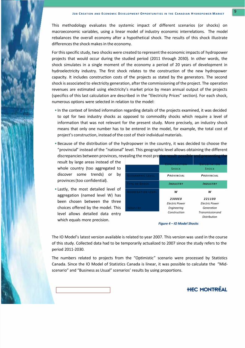
This methodology evaluates the systemic impact of different scenarios (or shocks) on

macroeconomic variables, using a linear model of industry economic interrelations. The model

rebalances the overall economy after a hypothetical shock. The results of this shock illustrate

differences the shock makes in the economy.

For this specific study, two shocks were created to represent the economic impacts of hydropower

projects that would occur during the studied period (2011 through 2030). In other words, the

shock simulates in a single moment of the economy a period of 20 years of development in

hydroelectricity industry. The first shock relates to the construction of the new hydropower

capacity. It includes construction costs of the projects as stated by the generators. The second

shock is associated to electricity generation, after the commissioning of the project. The operation

revenues are estimated using electricity’s market price by mean annual output of the projects

(specifics of this last calculation are described in the “Electricity Prices” section). For each shock,

numerous options were selected in relation to the model:

• In the context of limited information regarding details of the projects examined, it was decided

to opt for two industry shocks as opposed to commodity shocks which require a level of

information that was not relevant for the present study. More precisely, an industry shockmeans that only one number has to be entered in the model, for example, the total cost of

project’s construction, instead of the cost of their individual materials.

•

Because of the distribution of the hydropower in the country, it was decided to choose the

“provincial” instead of the “national” level. This geographic level allows obtaining the different

discrepancies between provinces, revealing the most precise result possible and presenting the

result by large areas instead of the

whole country (too aggregated to

discover some trends) or by

provinces (too confidential).

• Lastly, the most detailed level of

aggregation (named level W) has

been chosen between the three

choices offered by the model. This

level allows detailed data entry

which equals more precision.

The IO Model’s latest version available is related to year 2007. This version was used in the course

of this study. Collected data had to be temporarily actualized to 2007 since the study refers to theperiod 2011-2030.

The numbers related to projects from the “Optimistic” scenario were processed by Statistics

Canada. Since the IO Model of Statistics Canada is linear, it was possible to calculate the “Mid-

scenario” and “Business as Usual” scenarios’ results by using proportions.

Figure 4 – IO Model Shocks




The scenarios elaborated do

not take into account that

the conditions of market

may change and promote

hydropower development

S C E N A R I O S D E S C R I P T I O N

O P T I M I S T I C P R O J E C T S W I T H L E S S T H A N 5 0 % C H A N C E S O F

B E I N G R E A L I Z E D W I T H I N 2 0 Y E A R S

M I D - S C E N A R I O P R O J E C T S W I T H M O R E T H A N 5 0 % C H A N C E S

O F B E I N G R E A L I Z E D W I T H I N 2 0 Y E A R S

B U S I N E S S A S U S U A L A P P R O V E D P R O J E C T S

S C E N A R I O S

From the information gathered, three different scenarios were built: “Business as Usual”, “Mid-

scenario” and “Optimistic” scenario. Those scenarios correspond to the likelihood of the projects

to proceed. Three methods were selected to distribute the different projects between the

scenarios.

The first method was based onthe comments of the generators

who answered the questionnaire.

As guidelines, the generators

were given some criteria to define

their projects. The “Business as

Usual” scenario refers to projects

that have already been approved

or are in the process of being

approved. The “Mid-scenario” is associated to projects that have more than 50% likelihood of

proceeding within a 20-year period. Finally, the “Optimistic” scenario represents projects that

have less than 50% chance of being built, but which are still on the drawing boards of the

generators. Sometimes, the generators did qualify the likelihood of projects happening, which

means that the researchers made judgment calls to categorize projects.

The second methodology adopted is quite different from the first one and has been used for less

than 9% of projects. In cases where generators did not qualify the likelihood of the projects, it was

determined that projects that cost less than $3,000,000 per MW were “Business as Usual”, those

within $3,000,000 and $4,000,000 per MW were “Mid-scenario” and more than $4,000,000 per

MW were “Optimistic” scenario. These categories were established in accordance to two industry

experts.Finally, for the small hydro capacity, a third

methodology was used as those projects were

rarely mentioned by the generators. Therefore,

the assumptions regarding the likelihood of

happening of small projects were based on the

growth rate provided in an EIA report of 2010

(EIA, 2010). This report stated that: “The current

small hydro capacity in Canada is approximately

3,400 MW, and new capacity is growing at a rate

of 50 to 150 MW per year. It is estimated that about 15% of the identified small hydro potential of15,000 MW would be strong candidates for development under current socio-economic conditions

and with existing state-of-the-art technologies.” Based on this growing rate, a 50 MW per year was

assumed for the “Business as Usual” scenario, a 150 MW per year for the “Mid-Scenario” and a

250 MW per year for the “Optimistic” scenario. These scenarios imply that, under the “Optimistic”

scenario, more than twice the currently commercially viable small hydro projects would be built

during the next 20 years.

Figure 5 – Hydropower Projects Scenarios




For each scenario,

different electricity

prices projections

were compared in

order to validate the

EIA projections

Since the likelihood of projects was determined by the generators, no economic nor legislative

assumptions were made in order to justify which projects should emerge during the next 20 years.

On the other hand, it must be noted that many events could happen and increase the pace of

hydro projects development:

•

The price of coal, natural gas or other energy type could increase substantially thus fostering

hydropower projects;

• Provincial government could adopt rules that promote clean energy which include hydropower,

as seen in British Columbia;

• New technologies could be commercialized reducing the cost of projects that could become

profitable; and,

• New international agreements (following Kyoto Protocol) could be achieved or international

carbon market could be implemented.

Any similar event could favour hydropower development which implies that generators’ pending

projects could emerge and turn out to be commercially viable. On the other hand, other eventscould happen and disadvantage hydro project development, like unfavorable government policies.

C O N S T R U C T I O N C O S T E S T I M A T I O N

In order to evaluate the economic impact of hydropower projects construction planned for the

next 20 years, the information on construction costs was taken directly from the generators.

O P E R A T I N G R E V E N U E S E S T I M A T I O N - E L E C T R I C I T Y P R I C E S

In order to evaluate the economic impact of the operating phase of the entire hydropower

projects to be implemented, projections on electricity prices were required. The value of the

“operation shock” to be introduced into the IO Model was estimated by multiplying the meanannual output (in GWh) of each new installation to be built by the electricity prices projections.

Projections on electricity prices from 2010 through 2030 were provided by tables from EIA (EIA,

2011). More than 40 different economic scenarios have been developed by EIA to project different

electricity prices. For our “Business as Usual” scenario, the

EIA “Reference” scenario was chosen. For the “Optimistic”

scenario, the EIA “GHG price economy wide” scenario was

chosen. This scenario is defined by EIA as if: “Carbon

allowance fee is set at the level of the cost containment

provision as specified in both the American Power Act of

2010 and the American Clean Energy and Security Act of

2009”. For the “Mid-scenario”, an average of these two

estimates was used. The projections (in 2009 US cents per

kWh) are presented in Appendix C.




To ensure their validity, these projections were compared with an estimate of the electricity cost

based on natural gas combined cycle technology. This estimate, specific to Quebec, was provided

by Rio Tinto Alcan (RTA, 2011). In order to get prices representative of all Canadian regions, the

projections were corrected by using only half the fees related to transportation, distribution and

compression. No carbon taxes were considered and financial and other costs were excluded. In

order to make electricity price projections from 2010 through 2030, EIA projections (EIA, 2011) for

natural gas price were used. As for the electricity price projections produced by the EIA, the EIA

“Reference” scenario was chosen for our “Business as Usual” scenario and “GHG price economy

wide” scenario was chosen for our “Optimistic” scenario. In the same way, an average of these

two estimates was used for our “Mid-scenario”. The electricity price projections resulting from

these calculations were comparable to the EIA Projections directly for electricity prices. Thus, EIA

projections for electricity prices were preferred in the present study.

It is crucial to note that the IO Model of Statistics Canada would have needed the operation costs

instead of the operation revenues in order to have reliable results. In other words, the generators’

margin, which is unknown, was included in the numbers when it should not have been. Because of

this discrepancy in the methodology, the results from the matrix for GDP and jobs related to theoperation are higher than they should have been.

C A S H F L O W S C A L C U L A T I O N S & A S S U M P T I O N S

Since the cash flows considered in the analysis are occurring at different moments and since the IO

Model is valid for 2007, some financial adjustments were required:

• All cash flows from 2011 and subsequent years have been discounted back to 2007;

• Since the results from the IO Model shock are given in 2007 dollars, they have been converted

into 2011 dollars (i.e. capitalized to 2011);

• The rate used to adjust for the time value of money is the average of the daily series of 2007

Government of Canada benchmark bond yields for five years to long term period 1 as they are

reasonable predictors of the future risk-free rates, including inflation and opportunity cost

predictions. The average retained rate is 4.244%;

• Even though the investments will occur over a few years, summing every yearly investment

discounted back to 2007 is the same as summing every yearly investment discounted back to

2011 and then discounting that sum back to 2007. Hence, since the sum of the discounted cash

flows as of 2011 is already known, that amount only has to be discounted back to 2007;

• If the construction of a project was started before 2011, only what was left of the construction

period was included in the analysis. This is the case of 5.7% of the projects considered. For

small hydropower facilities, one year construction periods were used; and,

•

When calculating project revenues, all related cash flows were considered as perpetuities

starting on the commissioning date. This is based on the fact that hydroelectricity facilities last

up to 100 years when well maintained.

1 Series V39053, V39054, V39055 and V39056




D A T A A G G R E G A T I O N

Participants to the survey are protected by a non-disclosure agreement endorsed by HEC team

members.

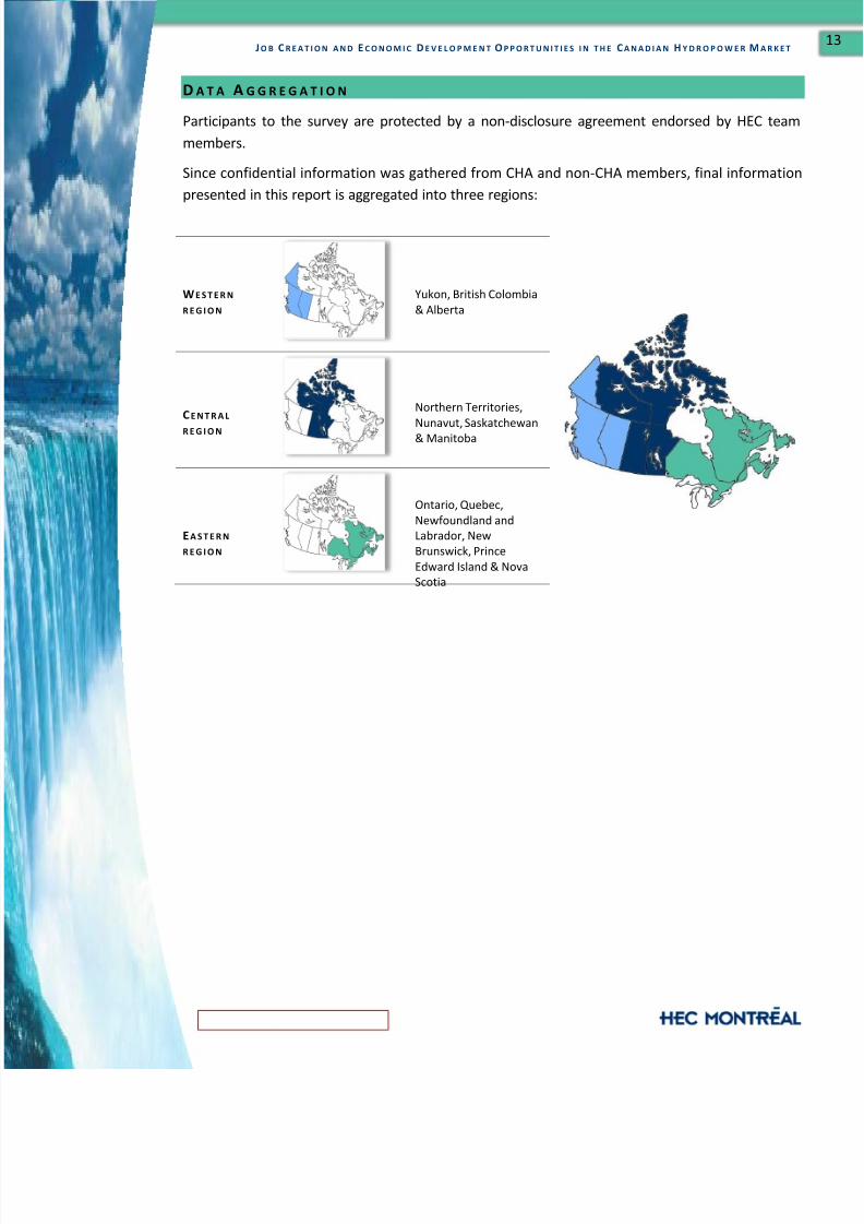
Since confidential information was gathered from CHA and non-CHA members, final information

presented in this report is aggregated into three regions:

WE S T E R N

R E G I O N Yukon, British Colombia

& Alberta

CE N T R A L

R E G I O N

Northern Territories,

Nunavut, Saskatchewan& Manitoba

EA S T E R N

R E G I O N

Ontario, Quebec,

Newfoundland and

Labrador, New

Brunswick, Prince

Edward Island & Nova

Scotia




C O L L E C T E D D A T A

With the integration of data from the generators and from the Internet, a total of 158 hydropower

projects for the next 20 years in Canada were identified (non-small hydro projects only). This

number is related to the “Optimistic” scenario. Among this, 24 projects correspond to the

“Business as Usual” scenario and 114 to the “Mid-scenario”. Most of the projects collected in the

“Optimistic” scenario are shared almost equally between the Western and the Eastern regions,

respectively 46% and 44% as presented hereafter. However, in the “Business as Usual” and

“Mid-scenario”, the Eastern region has more planned projects. For all scenarios, there are

significantly less projects in the Central region.

When comparing the three scenarios, the reader will notice that most hydropower projects in

Canada will be built only in the “Optimistic” scenario. This means that proactive government

policies would allow more projects to proceed.

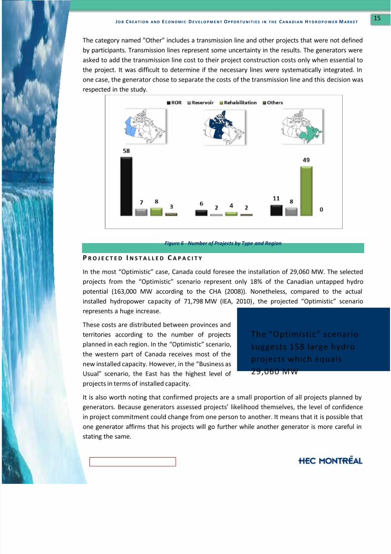
About a third of the 158 hydropower projects are upgrades or restorations. They are mainly

located in Eastern Canada, as presented at Figure 6. At this point, the reader should remember

that only the projects mentioned by the participants were included in the study. Therefore it is

possible that only a few participants chose to share this kind of projects (upgrades or restorations)

impacting the reliability of the data.

More than 80% of new constructions are run-of-rivers (ROR). Most ROR are concentrated in the

Western region while most storage hydro (reservoir) projects are located in the Eastern region.

The run-of-river projects usually have smaller installed capacities than storage hydro. As for the

Central region, it has few projects and does not distinguish itself in either category (ROR or

reservoir).




The “Optimistic” scenario

suggests 158 large hydro

projects which equals

29,060 MW

The category named "Other" includes a transmission line and other projects that were not defined

by participants. Transmission lines represent some uncertainty in the results. The generators were

asked to add the transmission line cost to their project construction costs only when essential to

the project. It was difficult to determine if the necessary lines were systematically integrated. In

one case, the generator chose to separate the costs of the transmission line and this decision was

respected in the study.

Figure 6 - Number of Projects by Type and Region

P R O J E C T E D I N S T A L L E D C A P A C I T Y

In the most “Optimistic” case, Canada could foresee the installation of 29,060 MW. The selected

projects from the “Optimistic” scenario represent only 18% of the Canadian untapped hydro

potential (163,000 MW according to the CHA (2008)). Nonetheless, compared to the actualinstalled hydropower capacity of 71,798 MW (IEA, 2010), the projected “Optimistic” scenario

represents a huge increase.

These costs are distributed between provinces and

territories according to the number of projects

planned in each region. In the “Optimistic” scenario,

the western part of Canada receives most of the

new installed capacity. However, in the “Business as

Usual” scenario, the East has the highest level of

projects in terms of installed capacity.

It is also worth noting that confirmed projects are a small proportion of all projects planned by

generators. Because generators assessed projects’ likelihood themselves, the level of confidence

in project commitment could change from one person to another. It means that it is possible that

one generator affirms that his projects will go further while another generator is more careful in

stating the same.




Figure 7 illustrate the planned installed capacity for the different regions.

Figure 7 - Installed Capacity by Region and Scenario

C O N S T R U C T I O N C A S H F L O W S

The 158 hydropower projects planned between 2011 and 2030 in the “Optimistic” scenario

represents an investment of $127 billion (in 2011 dollars for all this section of the report).

However, these data do not include small hydro projects. The following graph illustrates

construction costs for the different regions:

Figure 8 - Construction Costs by Region and Scenario




Figure 9 - Construction Costs per Scenario and Region

The construction cost associated to each region is quite representative of the number of projects

in each region. Thus, it is no surprise that, in the “Optimistic” scenario, the Western region has the

highest construction cost at $53.7 billion, while the Eastern region has $46.2 billion, and the

Central region, $27.8 billion.

In the “Business as Usual” scenario, it is noticeable that there is a concentration of project costs in

the Eastern region simply because most projects have already been approved in this region.

Projects gathered across the country are presenting a wide range of construction costs per MW.

Projects lower than $50 million are typically restoration or upgrade of existing facilities and add

little or no new capacity. The construction cost per MW ratio by region is presented at figure 10.

The variability of the ratio could be related to:

• The size of the project;

• The distance between the project location and the transmission infrastructure;

•

The distance between the project location and cities;

•

The topography;• The necessity for deforestation; and,

• The total annual output of the hydro infrastructure.

Figure 10 – Cost per MW Installed by Region ( “Optimistic” scenario)

According to some hydroelectricity experts interviewed, the wide variability of construction costs

per installed capacity could be expected. When observing important differences, profitability of




projects should be taken into account. Indeed, a project with a high cost per installed capacity

could generate an important mean annual output and associated revenues while the opposite is

also true. Also, it must be noted that the type of project does not influence the IO Model’s

calculations. Therefore, according to the Model, a dollar spent on a small hydropower project or

on a big one would create the same number of jobs and generate the same GDP value.

O P E R A T I O N R E V E N U E S If all the projects from the “Optimistic” scenario proceed in the next 20 years, their operation

would represent additional revenues of $172.4 billion for Canada (in 2011 adjusted dollars,

regardless of when the project goes into service for all this section of the report). However, these

data do not include the small hydro projects. The following graph illustrates the operation

revenues for the different regions:

Figure 11 - Operation Revenues by Region and Scenario

Figure 12 – Operation Revenues by Scenario and Region

The commissioning dates of the approved projects are scheduled in the next few years. Since most

approved projects are located in the Eastern region, most of the revenues from the "Business as

Usual" scenario are in this region. On the other hand, in the "Optimistic" scenario, the Western

region generates 52% of the revenues.




Because the revenues of each new facility have been calculated for a 100-year period, it is possible

to compare all projects without considering the moment of their construction. To make it the

comparison more relevant, it is possible to compare ratios of revenues per installed capacity, as

presented hereafter. This figure illustrates that revenues per MW differ from region to region. The

time value of money can partially explain the differences observed as western projects tend to

have later dates of commissioning. However, further research would be required to give a

comprehensive explanation.

Figure 13 – Revenues per MW Installed by Region ( “Optimistic” scenario)

M E A N A N N U A L O U T P U T

Even though the installed hydro capacity is important data, the mean annual output is even more

important since it represents the amount of energy that can be produced annually. This energy is

the source of revenues for generators.

Based on the collected data, the Canadian hydropower output would increase by 137 TWh in the

coming 20 years in the “Optimistic” scenario. This represents an important increase in comparison

to the actual mean annual output of hydroelectricity in Canada of 335 TWh (CHA, 2008). There is

an important difference between this “Optimistic” scenario and the 31 TWh of the “Business as

Usual” scenario. It is interesting to note that the “Business as Usual” scenario is presenting the

Eastern region as the first producer, with 66% of the global output, while the “Optimistic” scenario

is presenting the Western region as the first producer, with 53% of the global output.

Figure 14 - Mean Annual Output per Region




Depending on multiple factors like the hydro potential available in a specific region or the specific

capability regarding the installation to be built (base load or more peak power), a wide variability

of the “Energy produced per $ million” ratio can be observed. As presented in the following chart

and based on the “Optimistic” scenario, 1.34 GWh can be produced in the Central region with an

amount of $1 million since 1.54 GWh and 1.45 GWh would be produced with the same amount of

money in the Western and the Eastern regions respectively. The Central region’s ratio is slightly

lower and could be explained by the fact that the territory is less suitable for hydropower

development. The Western and Eastern regions have close ratios. The small difference observed

could be caused by a variety of reasons including differences in the generators’ assessments.

Figure 15 - Mean Annual Output per M$ of Investment (“ Optimistic ” Scenario)




In the “Optimistic”

scenario, the construction

investment would

generate 1,036,564 FTE

jobs

R E S U L T S

Statistics Canada provided the model output after the construction and operation shocks. Among

the results received, the study focused on the differences induced by the projects in terms of jobs

and GDP.

For these two indicators, the IO Model calculated the direct, indirect and induced effects of theprojects. Direct impacts measure the variation either in employment or GDP generated by either

investment in hydropower construction or revenues of operation. Indirect impacts represent the

changes due to inter-industry purchases in response to the new demand from the hydropower

industry associates. Finally, induced impacts measure the increase in the production of goods and

services in response to hydropower industry workers’ consumption and expenses.

P R O J E C T E D F U L L T I M E E Q U I V A L E N T J O B S

The following graphs represent the number of full-time equivalents (FTE) in Canada, between 2011

and 2030, related to the shocks. These data have been extracted from the results provided by the

IO Model of Statistics Canada. Since the model is linear, the number of FTE is proportional fromone scenario to the other. The number of FTE includes all direct, indirect and induced jobs.

The construction and operation of hydropower

projects for the 20 next years would create up to

1,754,473 FTE in an “Optimistic” scenario. It is

important to note that FTE are given in person-year

which means 1,754,473 FTE would be equivalent to

87,724 full-time jobs that would last for twenty

years. Because the number of jobs generated by the

operation of new hydropower facilities is inflated (due to the inclusion of generators’ margin in

the operating cost, as described in the methodology section), it is preferable to only take into

account FTE created by the construction of the projects. For the rest of this section, only the jobs

related to construction of hydropower projects will be considered, but the results of operation are

presented in the figures.

In the “Optimistic” scenario, the implementation of all 158 projects would create 1,036,564 FTE or

a mean of 51,828 FTE by year for 20 years. Knowing that according to Statistics Canada (2011a),

there are 17,401,000 workers in Canada, these 51,828 would represent 0.3% of the workforce.




FTE Operation

FTE Construction

T o t a l

FTE Operation

FTE Construction

T o t a l

FTE Operation

FTE Construction

T o t a l

v

Figure 16 - FTE Employment Creation in the Western Region

Figure 17 - FTE Employment Creation in Central Region

Figure 18 - FTE Employment Creation in Eastern Region




In the “Optimistic” scenario, construction related jobs would be created in proportion of the

added capacity, respectively: 45% would be in the Western region, 36% in the Eastern region and

20% in the Central region. Since 79.5% of the construction costs of the planned projects are

concentrated in the Eastern region in the “Business as Usual” scenario, it is no surprise that most

FTE are located in this region (85%).

It might be interesting to compare the number of FTE given by the IO matrix to other industries.

There are:

• 1.22 million workers in the construction industry;

• 1.74 million workers in the manufacturing industry; and,

• 329 thousands workers in the natural resources2 industry.

According to Statistics Canada (2011c), "The energy sector is vital to the nation’s economy,

accounting for 6.8% of gross domestic product (GDP) in 2008 and directly employing

363,000 people, or about 2% of the labour force".

It might also be interesting to compare the number of FTE given by the matrix for this study toother studies:

•

In an American study called “Job creation opportunities in hydropower”, Navigant Consulting

(2009) found that the installation of 60,000 MW of capacity could create up to 700,000 jobs.

When comparing these studies, it is important to remember that Navigant (2009) is considering

only direct and indirect jobs while this study considers direct, indirect and induced jobs. The

methodology used in Navigant study is also different than in this study. Even taking that into

account, the difference is important with the 29,060 MW and 1,036,563 FTE of this study.

• In a North-American study on “Employment and economic benefits of transmission

infrastructure investment in the US and Canada”, Wires and the Brattle Group (2011) found:”Ifthe $1 billion is spent over the course of one year, this means this investment will support

approximately 13,000 FTE jobs that year” (p.ii). When comparing this study to the present one,

the reader will note that Wires and the Brattle Group also find less jobs (if we do the

calculation, we find 17,133 jobs per billion for this study in the “Optimistic” scenario).

Reasons explaining these differences could include the fact that many Canadian projects are built

up North, in areas with high unemployment rates. Thus, it is possible that Canadian projects create

more jobs than projects in the United States, where more people could transfer from one job to

an hydro job. Other explanations for the differences observed are mentioned in the “Collected

data” section (cost per MW).

2 Forestry, fishing, mining, quarrying, oil and gas




In the “Optimistic”

scenario, the hydro

projects construction

would increase the

Canadian GDP by

$130,231 million

G R O S S D O M E S T I C P R O D U C T

The following graphs show the GDP increase generated in Canada by the planned hydropower

projects for the next 20 years for the different regions. The construction and operation of the

projects would increase the GDP of Canada by $313,340 million in the “Optimistic” scenario,

$221,678 million in the “Mid-scenario” and $76,162 million in the “Business as Usual” scenario.

The numbers include all direct, indirect and induced dollars generated by the industry.Similarly to the FTE section, it should be noted that the reliability of the value added to the GDP

generated by the operation of new hydropower facility is inflated. Therefore, it is preferable to

take into account only the GDP created by the construction of the projects. For the rest of this

section, only the GDP related to construction of hydropower projects will be considered. However,

the results of operation are presented in the figures.

In the “Optimistic” scenario, the construction of all

projects would generate $130,231 million or a mean of

$6,512 million by year for 20 years. According to

Statistics Canada, the current GDP (adjusted for the first

quarter of 2011) is $1,696,724 million at current price

(2011b). So if we compare the “Optimistic” GDP increase

equivalent for one year to the current GDP, it would

represent 0.38% of it.

In the “Optimistic” scenario, the GDP would increase

more in regions where more capacity is added. 42% of

the increase would be seen in the Eastern region, 41% in the Western region and 17% in the

Central region. This GDP distribution is similar to the distribution of FTE.

Although the model estimates that the GDP would be increased by projects, the real increase

could be superior to the study estimate. In fact, since the IO model is based on 2007 and since the

hydroelectricity exportation level was low at that time, a potentially higher level of exportation in

the future would have an even more positive effect on the GDP. It is also possible that the level of

hydropower construction was low in 2007 or that the projects built were small; if this was the

case, the multiplication factors would also be low, underestimating the GDP increase.




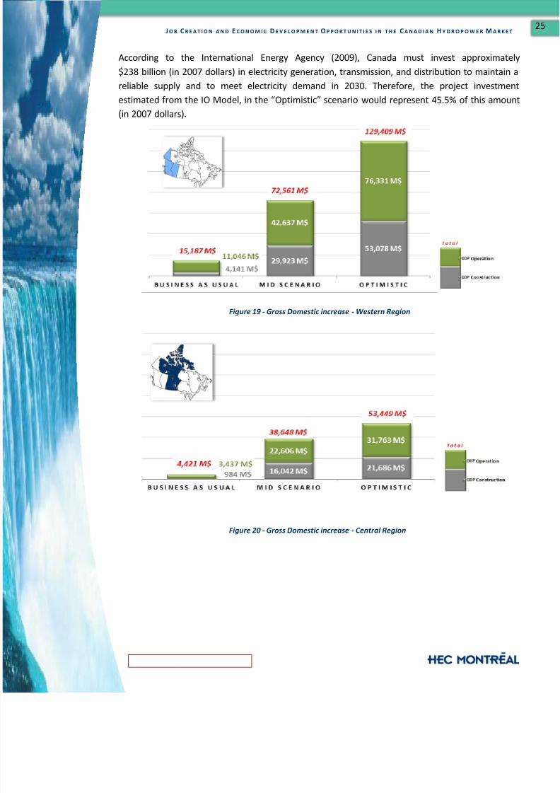
According to the International Energy Agency (2009), Canada must invest approximately

$238 billion (in 2007 dollars) in electricity generation, transmission, and distribution to maintain a

reliable supply and to meet electricity demand in 2030. Therefore, the project investment

estimated from the IO Model, in the “Optimistic” scenario would represent 45.5% of this amount

(in 2007 dollars).

Figure 19 - Gross Domestic increase - Western Region

Figure 20 - Gross Domestic increase - Central Region




Important note: The shocks simulated by the IO Model were related to very specific industries:“Electric power engineering construction” for the construction shock and “Electric power

generation transmission and distribution” for the operation shock. These industries were the most

representative we could use, but include a wider range of activities than the ones we were

interested in. For example, “Electric power engineering construction” includes not only

hydroelectricity, but several other electricity sources: natural gas, coal and nuclear. Since the

model calculates the mean economic impact of all electric power engineering constructions, it

could be somewhat different from the impact of hydroelectric constructions only.

In the same way, the industry “Electric power generation transportation and distribution” includes

the transport and distribution, while the value of the shock is considering only the production of

electricity. This limitation related to the precision of the operation shock could have produced

somewhat overestimated results, in terms of GDP and job created.

Figure 21 - Gross Domestic Creation - Eastern Region




C O N C L U S I O N

This report presents the results of the “Job Creation and Economic Development Opportunities in

the Canadian Hydropower Market Study”. This study has been conducted for the CHA by a team of

MBA students from HEC Montréal. The purpose was to determine the job creation as well as the

GDP increase which can be projected from construction and operation shocks in the hydropower

industry in Canada. It is important to consider that several limitations have been listed. However,

the number of responses, the methodology used, as well as the quantity of data gathered ensures

high quality, consistent results.

To enhance result analysis, three different scenarios were built: “Business as Usual”, “Mid” and

“Optimistic” scenarios which were based on projects’ likelihood. In order to respect the

confidentiality of the data collected from generators, the results have been aggregated into three

regions: the Western region (Yukon, British Colombia & Alberta), Central region (Northern

Territories, Nunavut, Saskatchewan & Manitoba) and Eastern region (Ontario, Quebec and Atlantic

Canada).

A total of 158 hydropower projects for the next 20 years for Canada were identified (excluding

small hydro projects). The data indicate that the projects are split almost equally between the

Western and the Eastern regions of Canada. About a third of the projects are upgrades or

restorations, mainly located in Eastern Canada. More than 80% of new constructions are run-of-

rivers (mostly concentrated in the Western region) while most storage hydro projects are located

in the Eastern region. In the “Optimistic” case, Canada could foresee the installation of 29,060 MW

of capacity which represents an investment of $127,745 million (in 2011 dollars). Based on the

collected data, the Canadian hydropower output would increase by 137 TWh in the coming 20

years in the event of an “Optimistic” scenario.

The construction of hydropower projects would create up to 1,036,564 FTE which is equivalent to51,828 full-time jobs that would last for twenty years. This would represent 0.3% of the 2010

Canadian workforce. In the “Optimistic” scenario, this would also increase the yearly Canadian

GDP by 0.38% and could represent up to 45% of the global estimated investment in the electricity

sector required by 2030.

Due to a short mandate timeframe (five weeks), it could be relevant for future studies to plan a

longer data gathering period to make sure that data are as comprehensive as possible. Also, a

longer data gathering period would enable more data cross checks, interviews and benchmarking.




Also, it might be appropriate to have a look at other criteria that could be included in other studies

like:

• Hydroelectricity exportation opportunities to the United States of America;

• Quantitative analysis of measures that would support the development of the hydropower (i.e.

carbon tax, policies that would promote green energy, etc.);

• Calculation of the profitability of the hydro projects considered for the study;

•

Analysis of how Canada could capitalize on its huge hydropower potential of 163,000 MW (list

the technological barriers and the theoretical potential that will never be exploited); and,

• Use of several economical and statistical tools to build different scenarios and project results.

Even if numbers can be analyzed and discussed extensively, this study reinforces the fact that

Canada is one of the most important hydropower producers in the world and it has the potential

to maintain that position for decades. However, water is a fragile resource and the exploitation of

rivers has to be done in a way that would suit Canadians and in partnership with governments.

Finally, if market conditions (economically, politically or socially) changed, it could promote even

more hydropower development and thus generate more economic benefits for Canada than

stated in this study.




L I S T O F F I G U R E S

FIGURE 1 – ELECTRICITY GENERATION IN CANADA BY SOURCES (STATISTICS CANADA, 2011B) ........................................PAGE 4

FIGURE 2 – CANADIAN ELECTRICITY GENERATION, 1990-2009 (NATURAL RESOURCES CANADA, 2011)..........................PAGE 4

FIGURE 3 – CANADIAN HYDROPOWER PLANT (CENTRE FOR ENERGY, 2011)................................................................PAGE 5

FIGURE 4 – IO MODEL SHOCKS ...........................................................................................................................PAGE 9

FIGURE 5 – HYDROPOWER PROJECTS SCENARIOS ..................................................................................................PAGE 10

FIGURE 6 - NUMBER OF PROJECTS BY TYPE AND REGION ........................................................................................PAGE 15

FIGURE 7 - INSTALLED CAPACITY BY REGION AND SCENARIO ....................................................................................PAGE 16

FIGURE 8 - CONSTRUCTION COSTS BY REGION AND SCENARIO .................................................................................PAGE 16

FIGURE 9 - CONSTRUCTION COSTS PER SCENARIO AND REGION ...............................................................................PAGE 17

FIGURE 10 – COST PER MW INSTALLED BY REGION (“OPTIMISTIC” SCENARIO) ..........................................................PAGE 17

FIGURE 11 - EXPLOITATION REVENUES BY REGION AND SCENARIO ...........................................................................PAGE 18

FIGURE 12 – EXPLOITATION REVENUES BY SCENARIO AND REGION ..........................................................................PAGE 18

FIGURE 13 – REVENUES PER MW INSTALLED BY REGION (“OPTIMISTIC” SCENARIO) ...................................................PAGE 19

FIGURE 14 - MEAN ANNUAL OUTPUT PER REGION ...............................................................................................PAGE 19

FIGURE 15 - MEAN ANNUAL OUTPUT PER M$ OF INVESTMENT (“OPTIMISTIC” SCENARIO) ..........................................PAGE 20

FIGURE 18 - FTE EMPLOYMENT CREATION IN THE WESTERN REGION .......................................................................PAGE 22

FIGURE 19 - FTE EMPLOYMENT CREATION IN CENTRAL REGION ..............................................................................PAGE 22

FIGURE 20 - FTE EMPLOYMENT CREATION IN EASTERN REGION ..............................................................................PAGE 22

FIGURE 19 - GROSS DOMESTIC INCREASE - WESTERN REGION ................................................................................PAGE 25

FIGURE 22 - GROSS DOMESTIC INCREASE - CENTRAL REGION ..................................................................................PAGE 25

FIGURE 23 - GROSS DOMESTIC CREATION - EASTERN REGION .................................................................................PAGE 26

http://wss.hec.ca/mba/2010-2011/94208767/Documents%20partages/CHA_Report_MASTER_vendredi%20v4.docx#_Toc300321185






































































































































































































G L O S S A R Y

Terms / Acronyms Definitions

EIA United States Energy Information Administration

FTE Full time equivalent, in person-year of employment

GDP Gross domestic product

GHG Greenhouse gas

GWh Giga watt hour, a unit of energy (the output of a hydro

installation) representing 109 Wh

Hydropower Production of electricity with waterpower

Hydropower potential Possible development of new production of electricity withwaterpower.

IEA International Energy Agency

Installed capacity The measure of a hydropower project’s electric generating

capacity at full production, usually measured in megawatts (MW)

IO Input Output Model

kWh Kilowatt hour, a unit of energy equal to 103 Watt hour

Mean annual output Frequently expressed in GWh, represent the quantity of

electricity produced by an installation during a year

MW Mega-watt, a unit of capacity of a hydro installation, equal to

109 Watts

ROR Run-of-river installation

Small hydropower project Project with an installed capacity below 10 MW

TWh Tera-watt hour, a unit of energy (the output of a hydro

installation) representing 1012 Wh




R E F E R E N C E S

BANK OF CANADA (2011). Site visited July 19, 2011: http://www.bankofcanada.ca .

BC HYDRO (2011). BC Hydro Clean Power Call . Document read on July 25, 2011 :

http://www.bchydro.com/etc/medialib/internet/documents/planning_regulatory/acquiring_powe

r/third_group_clean_power_call_project_overviews.Par.0001.File.third_group_clean_power_call_

project_overviews.pdf .

CANADIAN ELECTRICITY AGENCY (2009). Key Canadian Electricity Statistics. Site visited July 19, 2011:

http://www.electricity.ca/media/Industry%20Data%20July%202010/Key%20Canadian%20Electrici

ty%20Statistics.pdf .

CANADIAN HYDROELECTRICITY ASSOCIATION (2008). L’hydroélectricité au Canada: Passé, present et

avenir . Site visited July 19, 2011 :

http://www.canhydropower.org/hydro_fr/pdf/hydropower_past_present_future_fr.pdf .

CENTRE FOR ENERGY (2011). Site visited July 19, 2011:

http://www.centreforenergy.com/AboutEnergy/Hydro/ChartsIllustrations.asp .

EEM (2006). Study of the Hydropower Potential in Canada. 31 pages.

EIA (2011). Annual Energy Outlook 2011 with Projections to 2035. Site visited July 19, 2011:

http://www.easterncoalcouncil.net/PDF_Files/ANNUAL_ENERGY_OUTLOOK_20110383(2011).pdf .

INTERNATIONAL ENERGY AGENCY (2010). Small Scale Hydro – Public Policy & Experience Country Report

for Canada. 147 pages. Site visited July 19, 2011: http://canmetenergy-canmetenergie.nrcan-

rncan.gc.ca/fichier.php/codectec/En/2009_Hydro_02/CanadaSmallHydroPolicyFINAL_Updates_wi

th_appendix.pdf .

INNERGEX (2011). Site visited July 25, 2011: http://www.innergex.com/northwest-stave-river .

MANITOBA HYDRO (2011). Site visited July 8, 2011:

http://www.hydro.mb.ca/projects/bipoleIII/index.shtml?WT.mc_id=2606 .

NATURAL RESOURCES CANADA (2011). Site visited July 19, 2011:

http://www.nrcan.gc.ca/eneene/sources/eleele/abofai-eng.php#generation .

NAVIGANT CONSULTING (2009). Job creation opportunities in hydropower . Site visited July 19, 2011:http://hydro.org/wp-content/uploads/2010/12/NHA_JobsStudy_FinalReport.pdf .

RTA (2010). Renewable Power Generation Technology-Hydropower - Rio Tinto Energy and Climate

Strategy Energy Technology .

http://www.bankofcanada.ca/



http://www.bchydro.com/etc/medialib/internet/documents/planning_regulatory/acquiring_power/third_group_clean_power_call_project_overviews.Par.0001.File.third_group_clean_power_call_project_overviews.pdf




http://www.electricity.ca/media/Industry%20Data%20July%202010/Key%20Canadian%20Electricity%20Statistics.pdf



http://www.canhydropower.org/hydro_fr/pdf/hydropower_past_present_future_fr.pdf


http://www.centreforenergy.com/AboutEnergy/Hydro/ChartsIllustrations.asp


http://www.easterncoalcouncil.net/PDF_Files/ANNUAL_ENERGY_OUTLOOK_20110383(2011).pdf


http://canmetenergy-canmetenergie.nrcan-rncan.gc.ca/fichier.php/codectec/En/2009_Hydro_02/CanadaSmallHydroPolicyFINAL_Updates_with_appendix.pdf




http://www.innergex.com/northwest-stave-river



http://www.hydro.mb.ca/projects/bipoleIII/index.shtml?WT.mc_id=2606


http://www.nrcan.gc.ca/eneene/sources/eleele/abofai-eng.php#generation


http://hydro.org/wp-content/uploads/2010/12/NHA_JobsStudy_FinalReport.pdf





















RUSSELL, Ray (2011). Canada Hydropower: Liquid Cornerstone. Hydro Review. Site visited July 19,

2011: http://www.renewableenergyworld.com/rea/news/article/2011/04/canada-hydropower-

liquid-cornerstone.

STATISTICS CANADA (2009). User’s Guide to the Canadian Input Output Model : Industry Accounts

Division System of National Accounts Statistics Canada. 29 pages.

STATISTICS CANADA (2011a). Employment by industry . Document read on July 28, 2011.

STATISTICS CANADA (2011b). Economic and financial data. Document read on August 3, 2011:

http://www40.statcan.ca/101/cst01/DSBBCAN-eng.htm .

Statistics Canada (2011c)

http://www.statcan.gc.ca/pub/11-402-x/2010000/chap/ener/ener-eng.htm

WIRES AND THE BRATTLE GROUP (2011). Employment and economic benefits of transmission

infrastructure investment in the U.S. and Canada. Site visited July 19, 2011:

http://www.brattle.com/_documents/UploadLibrary/Upload947.pdf .

http://www.renewableenergyworld.com/rea/news/article/2011/04/canada-hydropower-liquid-cornerstone



http://www40.statcan.ca/101/cst01/DSBBCAN-eng.htm




http://www.brattle.com/_documents/UploadLibrary/Upload947.pdf










A P P E N D I X A – I N T E R V I E W E D O R G A N I Z A T I O N S

Interviewed CHA members:

AECOM

Atco Power Canada LtdBC Hydro

Brookfield Power

Cegertec

Columbia Power Corp.

Columbia Power Corp.

Dessau Inc.

Energy Ottawa Inc.

Fontaine Industries

Fortis Inc.

Hydro-Québec

Knight Piesold LtdManitoba Hydro

MWH Canada

Nalcor

Ontario Power Generation

Peter Kiewit Infrastructure

Reservoir Capital Corp.

Rio Tinto Alcan

SNC-Lavalin

Trans Alta

Trans Canada Corp.

Interviewed non-CHA members:

Sask Power

Yukon Energy




A P P E N D I X B – I N P U T - O U T P U T M O D E L L I M I T A T I O N

(The following text is from Statistics Canada documentation.)

The Canadian Input-Output Model is normally used to analyze the link between final demand and

industrial output levels. Two versions of the model are available: the national and the inter-

provincial. The input-output model provides a detailed breakdown of economic activities amongindustries and a detailed breakdown of industry outputs and inputs, including GDP components

and jobs, associated with any arbitrarily fixed exogenous demand. It also provides supply

requirements from other sources such as international or inter-provincial imports and impacts on

energy use and pollutant emissions associated with domestic production.

Direct, indirect and induced effects

The impact results are separated into direct and indirect effects. Induced effects are also included

in the national model but are still under development for the inter-provincial model. Figure 1

provides a schematic presentation of this differentiation of impacts. The direct impacts are the

deliveries by domestic industries and imports necessary to satisfy final demand expenditures onproducts and services. The indirect impacts cover upstream economic activities associated with

supplying intermediate inputs (the current expenditures on goods and services used up in the

production process) to the directly impacted industries. The induced impacts provide an estimate

of the production and imports associated with the spending of wages on consumption. The inter-

provincial input-output model has similar characteristics to the national version with the added

breakdown of the provincial and territorial dimension (and with the exception of the induced

effects).

Industry vs. final demand shocks

It is possible to specify shocks that bear directly on final expenditures (e.g., an investment projector a change in exports) or on the production of industries (e.g., current operation expenditure of a

factory). The latter production is considered to be delivered to final demand. Shocks applied to

commodities that do not form part of final demand or to industries that have no production in a

given province or territory cannot be submitted through the model.

Imports

The model provides the flexibility to control the direct allocation of the exogenous expenditure by

eliminating direct provincial and/or international imports in the case of a domestic final demand

shock. Thus, the effects of two investment projects of equal value can be analyzed with the input-

output model taking into account the origin of the equipment purchased (domestic or imported).

The projects can be compared in terms of their structural effects (relative impact on industry

output and the demand for jobs). While the model allows direct imports related to a domestic

final expenditure to be excluded from the impacts, imports that are embedded in intermediate

inputs or induced consumption expenditures cannot be excluded.




Valuation: purchaser vs. producer price shocks

Industry shocks are by definition valued at “producer” prices, i.e., factory gate prices. For final

expenditures, however, users have the flexibility to provide shock data in alternative valuation

bases: either in purchaser prices or in “producer” prices, i.e., respectively, including or excluding

commodity taxes, trade and transportation margins. In general, final expenditure shocks should be

in purchaser prices. For example, the impacts of car exports on the Canadian economy include not

only the value of the vehicles at the factory gate (“producer” price) but also the wholesaling and

transportation charges that bring the vehicles to the Canadian border. A shock on car exports in

purchaser price will provide an estimate of the impact on the wholesaling and transportation

industries. A shock on car exports in “producer” prices will assume the full impact of the shock is

concentrated on the automobile production industry.

Model closure

It should be noted that the models have an incomplete macroeconomic structure. In the inter-

provincial model, final demand is exogenous, while output is endogenous, and adjusts completely

to satisfy changes in any form of demand, whether final or by other industries. The exogeneity of

final demand is maintained in the model as there is no link between factor incomes (labour and

capital) and consumer demand or investment. There is also no link between taxes and government

expenditure. Thus, the inter-provincial IO model is an open input-output model, i.e., it is not

closed on the above-mentioned variables.

As a consequence, the total value-added generated from the open model will be less than the

initial demand shock. The total impact on income generated by the model is less than the value of

final demand by the amount of the leakages since that income is not fed back in the Keynesian

sense, i.e., re-spent on final demand expenditure to measure spin-off effects, which would add to

the direct and indirect impacts. The commodity leakages are basically composed of taxes on

products and imports.

Unlike the inter-provincial model, the national model is closed to wages and consumption

expenditures. Thus, it is a partially closed model. However, the relationship between wages and

consumption is complicated by other sources of revenues and expenditures for the personal

sector. These include revenues from other sources such as property income and transfers, outlays

for income taxes, and residual savings. The assumption used in this model is that consumption

constitutes a share of the total revenues of the personal sector. This implies that wages are spent

on consumption in the same proportion as all sources of revenue. For reference year 2005, the

share of consumption in the total revenues of the personal sector was approximately 70%.

However, within the personal sector, consumption levels and patterns are highly differentiatedand manifest a close dependence on several characteristics of the wage-earners such as education

and income levels, and geographic location. Creating an average relationship at the

macroeconomic level represents a simplifying assumption that blurs these distinctions and

thereby undermines the precision of the model results.




Impacts on jobs and the environment

Two other industry-based data sources are integrated into the model. These are the number of

jobs and the quantities of energy use and their associated pollutant emissions. The data on energy

use and emissions are only available at the national level and thus, they are only incorporated in

the national model.

The basic assumption underlying the use of these data in the model is that they maintain asomewhat linear relationship with gross output in the short term. The mixing of nominal output

values and physical quantities, however, entails some risks. This approach can be considered

sound if the value and quantity measures are for the same year and the analysis is focusing on the

structure of the economy for that same year. When used for projecting beyond the IO model year,

the relationship between values and quantities may be corrupted by the impact of price

variations. The farther the time horizon from the benchmark and the higher the price volatility in

the economy, the more important such considerations become. This problem may be attenuated

by converting model shocks into constant dollar shocks valued in the same base year as the IO

model year. Technological or regulatory changes beyond the IO model year may also have

substantial impacts on these components of the model.

Some other limitations of the model

The models also reflect a simplified macroeconomic structure. They do not include many variables

of interest for macroeconomic analysis such as the price level (or its rate of change: inflation),

interest rates and other financial variables. The models lack also important labour market

variables such as the labour force and unemployment rates.

The economic structure of these models being incomplete, the impact results they generate have

to be interpreted cautiously using extraneous information about the economic situation and the

nature of the shocks given. They only provide resource allocations associated with the given

shocks and do not tell if the resources will be available or will have to be diverted from other uses

in which case the impact, from a macroeconomic perspective, has to be scaled down.

The specification of equations in the input-output models is also simplified. More precisely, the

technical production relationships assume fixed coefficients (no substitution of inputs) which may

differ from the marginal coefficients over the short run. Therefore, the results must be interpreted

as corresponding to a long run equilibrium impact under constant returns to scale along a linear

expansion path.

In brief, the input-output model is a structural model dealing primarily with resource allocation in

the economy corresponding to an exogenously given demand. It does not provide an absolutely

exact measure of the impact of a shock on the level of use of resources in the economy. The

assessment of the impact of a shock on the level of resource utilization should be complemented

by extraneous judgement, i.e. expert judgment on the part of the users based on knowledge of

major macroeconomic links in and a good factual knowledge of the business cycle phase in which

the economy is evolving.




A P P E N D I X C – E L E C T R I C I T Y P R I C E S P R O J E C T I O N S

Production electricity market price (cent 2009 / KWh)

2011 2012 2013 2014 2015 2016 2017 2018 2019 2020 2021 2022 2023 2024 2025 2026 2027 2028 2029 2030 20

BUSINESS AS

USUAL 5,20 5,10 5,10 5,00 5,00 5,10 5,10 5,20 5,20 5,30 5,30 5,40 5,40 5,50 5,60 5,60 5,70 5,70 5,80 5,80 6,0

MID-SCENARIO 5,20 5,05 5,45 5,75 5,75 6,00 6,10 6,25 6,30 6,40 6,45 6,55 6,65 6,75 6,90 6,95 7,10 7,15 7,25 7,30 7,6

OPTIMISTIC 5,20 5,00 5,80 6,50 6,50 6,90 7,10 7,30 7,40 7,50 7,60 7,70 7,90 8,00 8,20 8,30 8,50 8,60 8,70 8,80 9

Source: (EIA, 2011).




A P P E N D I X D – D I R E C T , I N D I R E C T A N D I N D U C E D

I N T H E O P T I M I S T I C S C E N A R I O

Production Construction Total

Direct

impact

Direct +

indirect

impact

Direct,indirect+

induced

impact

Direct

impact

Direct +

indirect

impact

Direct,indirect +

induced

impact

Direct

impact

Direct +

indirect

impact

Diindi

ind

im

EAST 81,785 227,201 334,065 165,764 325,202 455,010 247,549 552,403 789

CENTER 69,025 91,240 121,385 117,428 165,585 203,573 186,453 256,825 324

WEST 78,214 189,974 262,459 132,458 285,076 377,981 210,672 475,050 640

TOTAL 229,024 508,415 717,909 415,650 775,863 1,036,564 644,674 1,284,278 1,75