cha2

Chapter 2

MATRICES

2.1 Matrix arithmetic

A matrix over a field F is a rectangular array of elements from F . The sym-bol Mm×n(F ) denotes the collection of all m× n matrices over F . Matriceswill usually be denoted by capital letters and the equation A = [aij ] meansthat the element in the i–th row and j–th column of the matrix A equalsaij . It is also occasionally convenient to write aij = (A)ij . For the present,all matrices will have rational entries, unless otherwise stated.

EXAMPLE 2.1.1 The formula aij = 1/(i + j) for 1 ≤ i ≤ 3, 1 ≤ j ≤ 4defines a 3× 4 matrix A = [aij ], namely

A =

1

2

1

3

1

4

1

5

1

3

1

4

1

5

1

6

1

4

1

5

1

6

1

7

.

DEFINITION 2.1.1 (Equality of matrices) MatricesA andB are saidto be equal if A and B have the same size and corresponding elements areequal; that is A and B ∈ Mm×n(F ) and A = [aij ], B = [bij ], with aij = bijfor 1 ≤ i ≤ m, 1 ≤ j ≤ n.

DEFINITION 2.1.2 (Addition of matrices) Let A = [aij ] and B =[bij ] be of the same size. Then A + B is the matrix obtained by addingcorresponding elements of A and B; that is

A+B = [aij ] + [bij ] = [aij + bij ].

23

24 CHAPTER 2. MATRICES

DEFINITION 2.1.3 (Scalar multiple of a matrix) Let A = [aij ] andt ∈ F (that is t is a scalar). Then tA is the matrix obtained by multiplyingall elements of A by t; that is

tA = t[aij ] = [taij ].

DEFINITION 2.1.4 (Additive inverse of a matrix) Let A = [aij ] .Then −A is the matrix obtained by replacing the elements of A by theiradditive inverses; that is

−A = −[aij ] = [−aij ].

DEFINITION 2.1.5 (Subtraction of matrices) Matrix subtraction isdefined for two matrices A = [aij ] and B = [bij ] of the same size, in theusual way; that is

A−B = [aij ]− [bij ] = [aij − bij ].

DEFINITION 2.1.6 (The zero matrix) For each m, n the matrix inMm×n(F ), all of whose elements are zero, is called the zero matrix (of sizem× n) and is denoted by the symbol 0.

The matrix operations of addition, scalar multiplication, additive inverseand subtraction satisfy the usual laws of arithmetic. (In what follows, s andt will be arbitrary scalars and A, B, C are matrices of the same size.)

1. (A+B) + C = A+ (B + C);

2. A+B = B +A;

3. 0 +A = A;

4. A+ (−A) = 0;

5. (s+ t)A = sA+ tA, (s− t)A = sA− tA;

6. t(A+B) = tA+ tB, t(A−B) = tA− tB;

7. s(tA) = (st)A;

8. 1A = A, 0A = 0, (−1)A = −A;

9. tA = 0⇒ t = 0 or A = 0.

Other similar properties will be used when needed.

2.1. MATRIX ARITHMETIC 25

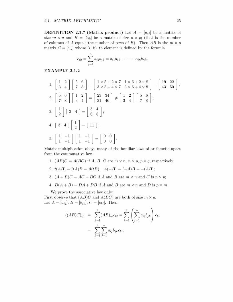
DEFINITION 2.1.7 (Matrix product) Let A = [aij ] be a matrix ofsize m × n and B = [bjk] be a matrix of size n × p; (that is the numberof columns of A equals the number of rows of B). Then AB is the m × pmatrix C = [cik] whose (i, k)–th element is defined by the formula

cik =n∑

j=1

aijbjk = ai1b1k + · · ·+ ainbnk.

EXAMPLE 2.1.2

1.

[

1 23 4

] [

5 67 8

]

=

[

1× 5 + 2× 7 1× 6 + 2× 83× 5 + 4× 7 3× 6 + 4× 8

]

=

[

19 2243 50

]

;

2.

[

5 67 8

] [

1 23 4

]

=

[

23 3431 46

]

6=[

1 23 4

] [

5 67 8

]

;

3.

[

12

]

[

3 4]

=

[

3 46 8

]

;

4.[

3 4]

[

12

]

=[

11]

;

5.

[

1 −11 −1

] [

1 −11 −1

]

=

[

0 00 0

]

.

Matrix multiplication obeys many of the familiar laws of arithmetic apartfrom the commutative law.

1. (AB)C = A(BC) if A, B, C are m× n, n× p, p× q, respectively;

2. t(AB) = (tA)B = A(tB), A(−B) = (−A)B = −(AB);

3. (A+B)C = AC +BC if A and B are m× n and C is n× p;

4. D(A+B) = DA+DB if A and B are m× n and D is p×m.We prove the associative law only:

First observe that (AB)C and A(BC) are both of size m× q.Let A = [aij ], B = [bjk], C = [ckl]. Then

((AB)C)il =

p∑

k=1

(AB)ikckl =

p∑

k=1

n∑

j=1

aijbjk

ckl

=

p∑

k=1

n∑

j=1

aijbjkckl.


Similarly

(A(BC))il =n∑

j=1

p∑

k=1

aijbjkckl.

However the double summations are equal. For sums of the form

n∑

j=1

p∑

k=1

djk and

p∑

k=1

n∑

j=1

djk

represent the sum of the np elements of the rectangular array [djk], by rowsand by columns, respectively. Consequently

((AB)C)il = (A(BC))il

for 1 ≤ i ≤ m, 1 ≤ l ≤ q. Hence (AB)C = A(BC).

The system of m linear equations in n unknowns

a11x1 + a12x2 + · · ·+ a1nxn = b1

a21x1 + a22x2 + · · ·+ a2nxn = b2...

am1x1 + am2x2 + · · ·+ amnxn = bm

is equivalent to a single matrix equation

a11 a12 · · · a1n

a21 a22 · · · a2n

......

am1 am2 · · · amn

x1

x2

...xn

=

b1b2...

bm

,

that is AX = B, where A = [aij ] is the coefficient matrix of the system,

X =

x1

x2

...xn

is the vector of unknowns and B =

b1b2...bm

is the vector of

constants.Another useful matrix equation equivalent to the above system of linear

equations is

x1

a11

a21

...am1

+ x2

a12

a22

...am2

+ · · ·+ xn

a1n

a2n

...amn

=

b1b2...bm

.

2.2. LINEAR TRANSFORMATIONS 27

EXAMPLE 2.1.3 The system

x+ y + z = 1

x− y + z = 0.

is equivalent to the matrix equation

[

1 1 11 −1 1

]

xyz

=

[

10

]

and to the equation

x

[

11

]

+ y

[

1−1

]

+ z

[

11

]

=

[

10

]

.

2.2 Linear transformations

An n–dimensional column vector is an n× 1 matrix over F . The collectionof all n–dimensional column vectors is denoted by F n.Every matrix is associated with an important type of function called a

linear transformation.

DEFINITION 2.2.1 (Linear transformation) WithA ∈Mm×n(F ), weassociate the function TA : Fn → Fm defined by TA(X) = AX for allX ∈ Fn. More explicitly, using components, the above function takes theform

y1 = a11x1 + a12x2 + · · ·+ a1nxn

y2 = a21x1 + a22x2 + · · ·+ a2nxn

...

ym = am1x1 + am2x2 + · · ·+ amnxn,

where y1, y2, · · · , ym are the components of the column vector TA(X).

The function just defined has the property that

TA(sX + tY ) = sTA(X) + tTA(Y ) (2.1)

for all s, t ∈ F and all n–dimensional column vectors X, Y . For

TA(sX + tY ) = A(sX + tY ) = s(AX) + t(AY ) = sTA(X) + tTA(Y ).


REMARK 2.2.1 It is easy to prove that if T : F n → Fm is a functionsatisfying equation 2.1, then T = TA, where A is the m × n matrix whosecolumns are T (E1), . . . , T (En), respectively, where E1, . . . , En are the n–dimensional unit vectors defined by

E1 =

10...0

, . . . , En =

00...1

.

One well–known example of a linear transformation arises from rotatingthe (x, y)–plane in 2-dimensional Euclidean space, anticlockwise through θradians. Here a point (x, y) will be transformed into the point (x1, y1),where

x1 = x cos θ − y sin θy1 = x sin θ + y cos θ.

In 3–dimensional Euclidean space, the equations

x1 = x cos θ − y sin θ, y1 = x sin θ + y cos θ, z1 = z;

x1 = x, y1 = y cosφ− z sinφ, z1 = y sinφ+ z cosφ;

x1 = x cosψ − z sinψ, y1 = y, z1 = x sinψ + z cosψ;

correspond to rotations about the positive z, x, y–axes, anticlockwise throughθ, φ, ψ radians, respectively.

The product of two matrices is related to the product of the correspond-ing linear transformations:

If A ism×n and B is n×p, then the function TATB : Fp → Fm, obtained

by first performing TB, then TA is in fact equal to the linear transformationTAB. For if X ∈ F p, we have

TATB(X) = A(BX) = (AB)X = TAB(X).

The following example is useful for producing rotations in 3–dimensionalanimated design. (See [27, pages 97–112].)

EXAMPLE 2.2.1 The linear transformation resulting from successivelyrotating 3–dimensional space about the positive z, x, y–axes, anticlockwisethrough θ, φ, ψ radians respectively, is equal to TABC , where

2.2. LINEAR TRANSFORMATIONS 29

θ

l

(x, y)

(x1, y1)

¡¡¡¡¡¡¡¡

¡¡

¡¡

¡

@@

@@

@@@

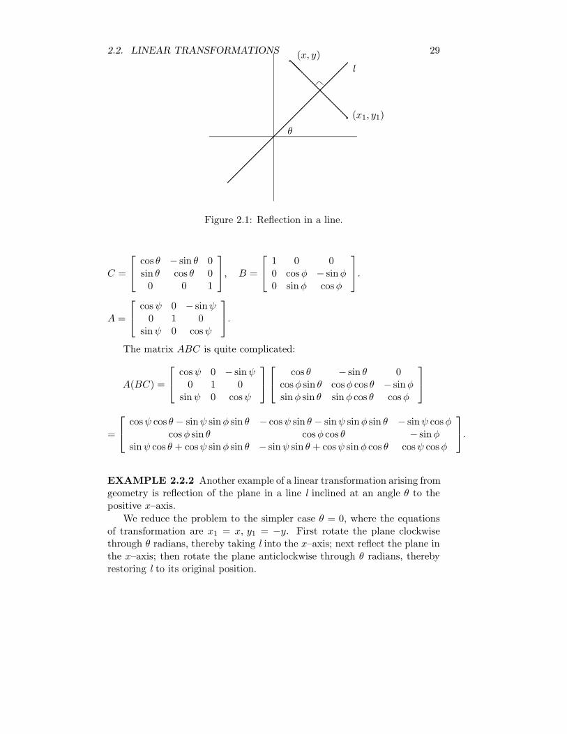
Figure 2.1: Reflection in a line.

C =

cos θ − sin θ 0sin θ cos θ 00 0 1

, B =

1 0 00 cosφ − sinφ0 sinφ cosφ

.

A =

cosψ 0 − sinψ0 1 0sinψ 0 cosψ

.

The matrix ABC is quite complicated:

A(BC) =

cosψ 0 − sinψ0 1 0sinψ 0 cosψ

cos θ − sin θ 0cosφ sin θ cosφ cos θ − sinφsinφ sin θ sinφ cos θ cosφ

=

cosψ cos θ − sinψ sinφ sin θ − cosψ sin θ − sinψ sinφ sin θ − sinψ cosφcosφ sin θ cosφ cos θ − sinφ

sinψ cos θ + cosψ sinφ sin θ − sinψ sin θ + cosψ sinφ cos θ cosψ cosφ

.

EXAMPLE 2.2.2 Another example of a linear transformation arising fromgeometry is reflection of the plane in a line l inclined at an angle θ to thepositive x–axis.

We reduce the problem to the simpler case θ = 0, where the equationsof transformation are x1 = x, y1 = −y. First rotate the plane clockwisethrough θ radians, thereby taking l into the x–axis; next reflect the plane inthe x–axis; then rotate the plane anticlockwise through θ radians, therebyrestoring l to its original position.


θ

l

(x, y)

(x1, y1)

¡¡¡¡¡¡¡¡

¡¡

¡¡

¡

@@

@

Figure 2.2: Projection on a line.

In terms of matrices, we get transformation equations

[

x1

y1

]

=

[

cos θ − sin θsin θ cos θ

] [

1 00 −1

] [

cos (−θ) − sin (−θ)sin (−θ) cos (−θ)

] [

xy

]

=

[

cos θ sin θsin θ − cos θ

] [

cos θ sin θ− sin θ cos θ

] [

xy

]

=

[

cos 2θ sin 2θsin 2θ − cos 2θ

] [

xy

]

.

The more general transformation

[

x1

y1

]

= a

[


] [

xy

]

+

[

uv

]

, a > 0,

represents a rotation, followed by a scaling and then by a translation. Suchtransformations are important in computer graphics. See [23, 24].

EXAMPLE 2.2.3 Our last example of a geometrical linear transformationarises from projecting the plane onto a line l through the origin, inclinedat angle θ to the positive x–axis. Again we reduce that problem to thesimpler case where l is the x–axis and the equations of transformation arex1 = x, y1 = 0.In terms of matrices, we get transformation equations

[

x1

y1

]

=

[


] [

1 00 0

] [

cos (−θ) − sin (−θ)sin (−θ) cos (−θ)

] [

xy

]

2.3. RECURRENCE RELATIONS 31

=

[

cos θ 0sin θ 0

] [

cos θ sin θ− sin θ cos θ

] [

xy

]

=

[

cos2 θ cos θ sin θsin θ cos θ sin2 θ

] [

xy

]

.

2.3 Recurrence relations

DEFINITION 2.3.1 (The identity matrix) The n × n matrix In =[δij ], defined by δij = 1 if i = j, δij = 0 if i 6= j, is called the n× n identitymatrix of order n. In other words, the columns of the identity matrix oforder n are the unit vectors E1, · · · , En, respectively.

For example, I2 =

[

1 00 1

]

.

THEOREM 2.3.1 If A is m× n, then ImA = A = AIn.

DEFINITION 2.3.2 (k–th power of a matrix) If A is an n×nmatrix,we define Ak recursively as follows: A0 = In and A

k+1 = AkA for k ≥ 0.

For example A1 = A0A = InA = A and hence A2 = A1A = AA.

The usual index laws hold provided AB = BA:

1. AmAn = Am+n, (Am)n = Amn;

2. (AB)n = AnBn;

3. AmBn = BnAm;

4. (A+B)2 = A2 + 2AB +B2;

5. (A+B)n =n∑

i=0

(

ni

)

AiBn−i;

6. (A+B)(A−B) = A2 −B2.

We now state a basic property of the natural numbers.

AXIOM 2.3.1 (PRINCIPLE OF MATHEMATICAL INDUCTION)If for each n ≥ 1, Pn denotes a mathematical statement and

(i) P1 is true,


(ii) the truth of Pn implies that of Pn+1 for each n ≥ 1,

then Pn is true for all n ≥ 1.

EXAMPLE 2.3.1 Let A =

[

7 4−9 −5

]

. Prove that

An =

[

1 + 6n 4n−9n 1− 6n

]

if n ≥ 1.

Solution. We use the principle of mathematical induction.

Take Pn to be the statement

An =

[

1 + 6n 4n−9n 1− 6n

]

.

Then P1 asserts that

A1 =

[

1 + 6× 1 4× 1−9× 1 1− 6× 1

]

=

[

7 4−9 −5

]

,

which is true. Now let n ≥ 1 and assume that Pn is true. We have to deducethat

An+1 =

[

1 + 6(n+ 1) 4(n+ 1)−9(n+ 1) 1− 6(n+ 1)

]

=

[

7 + 6n 4n+ 4−9n− 9 −5− 6n

]

.

Now

An+1 = AnA

=

[

1 + 6n 4n−9n 1− 6n

] [

7 4−9 −5

]

=

[

(1 + 6n)7 + (4n)(−9) (1 + 6n)4 + (4n)(−5)(−9n)7 + (1− 6n)(−9) (−9n)4 + (1− 6n)(−5)

]

=

[

7 + 6n 4n+ 4−9n− 9 −5− 6n

]

,

and “the induction goes through”.

The last example has an application to the solution of a system of re-currence relations:

2.4. PROBLEMS 33

EXAMPLE 2.3.2 The following system of recurrence relations holds forall n ≥ 0:

xn+1 = 7xn + 4yn

yn+1 = −9xn − 5yn.

Solve the system for xn and yn in terms of x0 and y0.

Solution. Combine the above equations into a single matrix equation[

xn+1

yn+1

]

=

[

7 4−9 −5

] [

xn

yn

]

,

or Xn+1 = AXn, where A =

[

7 4−9 −5

]

and Xn =

[

xn

yn

]

.

We see that

X1 = AX0

X2 = AX1 = A(AX0) = A2X0

...

Xn = AnX0.

(The truth of the equation Xn = AnX0 for n ≥ 1, strictly speakingfollows by mathematical induction; however for simple cases such as theabove, it is customary to omit the strict proof and supply instead a fewlines of motivation for the inductive statement.)Hence the previous example gives

[

xn

yn

]

= Xn =

[

1 + 6n 4n−9n 1− 6n

] [

x0

y0

]

=

[

(1 + 6n)x0 + (4n)y0

(−9n)x0 + (1− 6n)y0

]

,

and hence xn = (1+6n)x0+4ny0 and yn = (−9n)x0+(1−6n)y0, for n ≥ 1.

2.4 PROBLEMS

1. Let A, B, C, D be matrices defined by

A =

3 0−1 21 1

, B =

1 5 2−1 1 0−4 1 3

,


C =

−3 −12 14 3

, D =

[

4 −12 0

]

.

Which of the following matrices are defined? Compute those matriceswhich are defined.

A+B, A+ C, AB, BA, CD, DC, D2.

[Answers: A+ C, BA, CD, D2;

0 −11 35 4

,

0 12−4 2−10 5

,

−14 310 −222 −4

,

[

14 −48 −2

]

.]

2. Let A =

[

−1 0 10 1 1

]

. Show that if B is a 3× 2 such that AB = I2,

then

B =

a b−a− 1 1− ba+ 1 b

for suitable numbers a and b. Use the associative law to show that(BA)2B = B.

3. If A =

[

a bc d

]

, prove that A2 − (a+ d)A+ (ad− bc)I2 = 0.

4. If A =

[

4 −31 0

]

, use the fact A2 = 4A − 3I2 and mathematicalinduction, to prove that

An =(3n − 1)2

A+3− 3n2

I2 if n ≥ 1.

5. A sequence of numbers x1, x2, . . . , xn, . . . satisfies the recurrence rela-tion xn+1 = axn+bxn−1 for n ≥ 1, where a and b are constants. Provethat

[

xn+1

xn

]

= A

[

xn

xn−1

]

,

2.4. PROBLEMS 35

where A =

[

a b1 0

]

and hence express

[

xn+1

xn

]

in terms of

[

x1

x0

]

.

If a = 4 and b = −3, use the previous question to find a formula forxn in terms of x1 and x0.

[Answer:

xn =3n − 12

x1 +3− 3n2

x0.]

6. Let A =

[

2a −a2

1 0

]

.

(a) Prove that

An =

[

(n+ 1)an −nan+1

nan−1 (1− n)an

]

if n ≥ 1.

(b) A sequence x0, x1, . . . , xn, . . . satisfies the recurrence relation xn+1 =2axn− a2xn−1 for n ≥ 1. Use part (a) and the previous questionto prove that xn = nan−1x1 + (1− n)anx0 for n ≥ 1.

7. Let A =

[

a bc d

]

and suppose that λ1 and λ2 are the roots of the

quadratic polynomial x2−(a+d)x+ad−bc. (λ1 and λ2 may be equal.)

Let kn be defined by k0 = 0, k1 = 1 and for n ≥ 2

kn =n∑

i=1

λn−i1 λi−1

2 .

Prove thatkn+1 = (λ1 + λ2)kn − λ1λ2kn−1,

if n ≥ 1. Also prove that

kn =

{

(λn1 − λn

2 )/(λ1 − λ2) if λ1 6= λ2,

nλn−11 if λ1 = λ2.

Use mathematical induction to prove that if n ≥ 1,

An = knA− λ1λ2kn−1I2,

[Hint: Use the equation A2 = (a+ d)A− (ad− bc)I2.]


8. Use Question 7 to prove that if A =

[

1 22 1

]

, then

An =3n

2

[

1 11 1

]

+(−1)n−1

2

[

−1 11 −1

]

if n ≥ 1.

9. The Fibonacci numbers are defined by the equations F0 = 0, F1 = 1and Fn+1 = Fn + Fn−1 if n ≥ 1. Prove that

Fn =1√5

((

1 +√5

2

)n

−(

1−√5

2

)n)

if n ≥ 0.

10. Let r > 1 be an integer. Let a and b be arbitrary positive integers.Sequences xn and yn of positive integers are defined in terms of a andb by the recurrence relations

xn+1 = xn + ryn

yn+1 = xn + yn,

for n ≥ 0, where x0 = a and y0 = b.

Use Question 7 to prove that

xn

yn→√r as n→∞.

2.5 Non–singular matrices

DEFINITION 2.5.1 (Non–singular matrix)

A square matrix A ∈ Mn×n(F ) is called non–singular or invertible ifthere exists a matrix B ∈Mn×n(F ) such that

AB = In = BA.

Any matrix B with the above property is called an inverse of A. If A doesnot have an inverse, A is called singular.

2.5. NON–SINGULAR MATRICES 37

THEOREM 2.5.1 (Inverses are unique)

If A has inverses B and C, then B = C.

Proof. Let B and C be inverses of A. Then AB = In = BA and AC =In = CA. Then B(AC) = BIn = B and (BA)C = InC = C. Hence becauseB(AC) = (BA)C, we deduce that B = C.

REMARK 2.5.1 If A has an inverse, it is denoted by A−1. So

AA−1 = In = A−1A.

Also if A is non–singular, it follows that A−1 is also non–singular and

(A−1)−1 = A.

THEOREM 2.5.2 If A and B are non–singular matrices of the same size,then so is AB. Moreover

(AB)−1 = B−1A−1.

Proof.

(AB)(B−1A−1) = A(BB−1)A−1 = AInA−1 = AA−1 = In.

Similarly(B−1A−1)(AB) = In.

REMARK 2.5.2 The above result generalizes to a product of m non–singular matrices: If A1, . . . , Am are non–singular n× n matrices, then theproduct A1 . . . Am is also non–singular. Moreover

(A1 . . . Am)−1 = A−1

m . . . A−11 .

(Thus the inverse of the product equals the product of the inverses in thereverse order.)

EXAMPLE 2.5.1 If A and B are n × n matrices satisfying A2 = B2 =(AB)2 = In, prove that AB = BA.

Solution. Assume A2 = B2 = (AB)2 = In. Then A, B, AB are non–singular and A−1 = A, B−1 = B, (AB)−1 = AB.But (AB)−1 = B−1A−1 and hence AB = BA.


EXAMPLE 2.5.2 A =

[

1 24 8

]

is singular. For suppose B =

[

a bc d

]

is an inverse of A. Then the equation AB = I2 gives

[

1 24 8

] [

a bc d

]

=

[

1 00 1

]

and equating the corresponding elements of column 1 of both sides gives thesystem

a+ 2c = 1

4a+ 8c = 0

which is clearly inconsistent.

THEOREM 2.5.3 Let A =

[

a bc d

]

and ∆ = ad − bc 6= 0. Then A isnon–singular. Also

A−1 = ∆−1

[

d −b−c a

]

.

REMARK 2.5.3 The expression ad − bc is called the determinant of A

and is denoted by the symbols detA or

∣

∣

∣

∣

a bc d

∣

∣

∣

∣

.

Proof. Verify that the matrix B = ∆−1

[

d −b−c a

]

satisfies the equation

AB = I2 = BA.

EXAMPLE 2.5.3 Let

A =

0 1 00 0 15 0 0

.

Verify that A3 = 5I3, deduce that A is non–singular and find A−1.

Solution. After verifying that A3 = 5I3, we notice that

A

(

1

5A2

)

= I3 =

(

1

5A2

)

A.

Hence A is non–singular and A−1 = 1

5A2.


THEOREM 2.5.4 If the coefficient matrix A of a system of n equationsin n unknowns is non–singular, then the system AX = B has the uniquesolution X = A−1B.

Proof. Assume that A−1 exists.

1. (Uniqueness.) Assume that AX = B. Then

(A−1A)X = A−1B,

InX = A−1B,

X = A−1B.

2. (Existence.) Let X = A−1B. Then

AX = A(A−1B) = (AA−1)B = InB = B.

THEOREM 2.5.5 (Cramer’s rule for 2 equations in 2 unknowns)

The system

ax+ by = e

cx+ dy = f

has a unique solution if ∆ =

∣

∣

∣

∣

a bc d

∣

∣

∣

∣

6= 0, namely

x =∆1

∆, y =

∆2

∆,

where

∆1 =

∣

∣

∣

∣

e bf d

∣

∣

∣

∣

and ∆2 =

∣

∣

∣

∣

a ec f

∣

∣

∣

∣

.

Proof. Suppose ∆ 6= 0. Then A =[

a bc d

]

has inverse

A−1 = ∆−1

[

d −b−c a

]

and we know that the system

A

[

xy

]

=

[

ef

]


has the unique solution

[

xy

]

= A−1

[

ef

]

=1

∆

[

d −b−c a

] [

ef

]

=1

∆

[

de− bf−ce+ af

]

=1

∆

[

∆1

∆2

]

=

[

∆1/∆∆2/∆

]

.

Hence x = ∆1/∆, y = ∆2/∆.

COROLLARY 2.5.1 The homogeneous system

ax+ by = 0

cx+ dy = 0

has only the trivial solution if ∆ =

∣

∣

∣

∣

a bc d

∣

∣

∣

∣

6= 0.

EXAMPLE 2.5.4 The system

7x+ 8y = 100

2x− 9y = 10

has the unique solution x = ∆1/∆, y = ∆2/∆, where

∆ =

∣

∣

∣

∣

7 82 −9

∣

∣

∣

∣

= −79, ∆1 =

∣

∣

∣

∣

100 810 −9

∣

∣

∣

∣

= −980, ∆2 =

∣

∣

∣

∣

7 1002 10

∣

∣

∣

∣

= −130.

So x = 980

79and y = 130

79.

THEOREM 2.5.6 Let A be a square matrix. If A is non–singular, thehomogeneous system AX = 0 has only the trivial solution. Equivalently,if the homogenous system AX = 0 has a non–trivial solution, then A issingular.

Proof. If A is non–singular and AX = 0, then X = A−10 = 0.

REMARK 2.5.4 If A∗1, . . . , A∗n denote the columns of A, then the equa-tion

AX = x1A∗1 + . . .+ xnA∗n

holds. Consequently theorem 2.5.6 tells us that if there exist scalars x1, . . . , xn,not all zero, such that

x1A∗1 + . . .+ xnA∗n = 0,


that is, if the columns of A are linearly dependent, then A is singular. Anequivalent way of saying that the columns of A are linearly dependent is thatone of the columns of A is expressible as a sum of certain scalar multiplesof the remaining columns of A; that is one column is a linear combinationof the remaining columns.

EXAMPLE 2.5.5

A =

1 2 31 0 13 4 7

is singular. For it can be verified that A has reduced row–echelon form

1 0 10 1 10 0 0

and consequently AX = 0 has a non–trivial solution x = −1, y = −1, z = 1.

REMARK 2.5.5 More generally, if A is row–equivalent to a matrix con-taining a zero row, then A is singular. For then the homogeneous systemAX = 0 has a non–trivial solution.

An important class of non–singular matrices is that of the elementaryrow matrices.

DEFINITION 2.5.2 (Elementary row matrices) There are three types,Eij , Ei(t), Eij(t), corresponding to the three kinds of elementary row oper-ation:

1. Eij , (i 6= j) is obtained from the identity matrix In by interchangingrows i and j.

2. Ei(t), (t 6= 0) is obtained by multiplying the i–th row of In by t.

3. Eij(t), (i 6= j) is obtained from In by adding t times the j–th row ofIn to the i–th row.

EXAMPLE 2.5.6 (n = 3.)

E23 =

1 0 00 0 10 1 0

, E2(−1) =

1 0 00 −1 00 0 1

, E23(−1) =

1 0 00 1 −10 0 1

.


The elementary row matrices have the following distinguishing property:

THEOREM 2.5.7 If a matrix A is pre–multiplied by an elementary row–matrix, the resulting matrix is the one obtained by performing the corre-sponding elementary row–operation on A.

EXAMPLE 2.5.7

E23

a bc de f

=

1 0 00 0 10 1 0

a bc de f

=

a be fc d

.

COROLLARY 2.5.2 The three types of elementary row–matrices are non–singular. Indeed

1. E−1ij = Eij ;

2. E−1i (t) = Ei(t

−1);

3. (Eij(t))−1 = Eij(−t).

Proof. Taking A = In in the above theorem, we deduce the followingequations:

EijEij = In

Ei(t)Ei(t−1) = In = Ei(t

−1)Ei(t) if t 6= 0Eij(t)Eij(−t) = In = Eij(−t)Eij(t).

EXAMPLE 2.5.8 Find the 3 × 3 matrix A = E3(5)E23(2)E12 explicitly.Also find A−1.

Solution.

A = E3(5)E23(2)

0 1 01 0 00 0 1

= E3(5)

0 1 01 0 20 0 1

=

0 1 01 0 20 0 5

.

To find A−1, we have

A−1 = (E3(5)E23(2)E12)−1

= E−112 (E23(2))

−1 (E3(5))−1

= E12E23(−2)E3(5−1)


= E12E23(−2)

1 0 00 1 00 0 1

5

= E12

1 0 00 1 −2

5

0 0 1

5

=

0 1 −2

5

1 0 00 0 1

5

.

REMARK 2.5.6 Recall that A and B are row–equivalent if B is obtainedfrom A by a sequence of elementary row operations. If E1, . . . , Er are therespective corresponding elementary row matrices, then

B = Er (. . . (E2(E1A)) . . .) = (Er . . . E1)A = PA,

where P = Er . . . E1 is non–singular. Conversely if B = PA, where P isnon–singular, then A is row–equivalent to B. For as we shall now see, P isin fact a product of elementary row matrices.

THEOREM 2.5.8 Let A be non–singular n× n matrix. Then

(i) A is row–equivalent to In,

(ii) A is a product of elementary row matrices.

Proof. Assume that A is non–singular and let B be the reduced row–echelonform of A. Then B has no zero rows, for otherwise the equation AX = 0would have a non–trivial solution. Consequently B = In.

It follows that there exist elementary row matrices E1, . . . , Er such thatEr (. . . (E1A) . . .) = B = In and hence A = E−1

1 . . . E−1r , a product of

elementary row matrices.

THEOREM 2.5.9 Let A be n× n and suppose that A is row–equivalentto In. Then A is non–singular and A

−1 can be found by performing thesame sequence of elementary row operations on In as were used to convertA to In.

Proof. Suppose that Er . . . E1A = In. In other words BA = In, whereB = Er . . . E1 is non–singular. Then B

−1(BA) = B−1In and so A = B−1,which is non–singular.

Also A−1 =(

B−1)−1

= B = Er ((. . . (E1In) . . .), which shows that A−1

is obtained from In by performing the same sequence of elementary rowoperations as were used to convert A to In.


REMARK 2.5.7 It follows from theorem 2.5.9 that if A is singular, thenA is row–equivalent to a matrix whose last row is zero.

EXAMPLE 2.5.9 Show that A =

[

1 21 1

]

is non–singular, find A−1 and

express A as a product of elementary row matrices.

Solution. We form the partitionedmatrix [A|I2] which consists ofA followedby I2. Then any sequence of elementary row operations which reduces A toI2 will reduce I2 to A

−1. Here

[A|I2] =[

1 2 1 01 1 0 1

]

R2 → R2 −R1

[

1 2 1 00 −1 −1 1

]

R2 → (−1)R2

[

1 2 1 00 1 1 −1

]

R1 → R1 − 2R2

[

1 0 −1 20 1 1 −1

]

.

Hence A is row–equivalent to I2 and A is non–singular. Also

A−1 =

[

−1 21 −1

]

.

We also observe that

E12(−2)E2(−1)E21(−1)A = I2.

Hence

A−1 = E12(−2)E2(−1)E21(−1)A = E21(1)E2(−1)E12(2).

The next result is the converse of Theorem 2.5.6 and is useful for provingthe non–singularity of certain types of matrices.

THEOREM 2.5.10 Let A be an n × n matrix with the property thatthe homogeneous system AX = 0 has only the trivial solution. Then A isnon–singular. Equivalently, if A is singular, then the homogeneous systemAX = 0 has a non–trivial solution.


Proof. If A is n × n and the homogeneous system AX = 0 has only thetrivial solution, then it follows that the reduced row–echelon form B of Acannot have zero rows and must therefore be In. Hence A is non–singular.

COROLLARY 2.5.3 Suppose that A and B are n × n and AB = In.Then BA = In.

Proof. Let AB = In, where A and B are n × n. We first show that Bis non–singular. Assume BX = 0. Then A(BX) = A0 = 0, so (AB)X =0, InX = 0 and hence X = 0.Then from AB = In we deduce (AB)B

−1 = InB−1 and hence A = B−1.

The equation BB−1 = In then gives BA = In.

Before we give the next example of the above criterion for non-singularity,we introduce an important matrix operation.

DEFINITION 2.5.3 (The transpose of a matrix) Let A be an m×nmatrix. Then At, the transpose of A, is the matrix obtained by interchangingthe rows and columns of A. In other words if A = [aij ], then

(

At)

ji= aij .

Consequently At is n×m.

The transpose operation has the following properties:

1.(

At)t= A;

2. (A±B)t = At ±Bt if A and B are m× n;

3. (sA)t = sAt if s is a scalar;

4. (AB)t = BtAt if A is m× n and B is n× p;

5. If A is non–singular, then At is also non–singular and

(

At)−1

=(

A−1)t;

6. XtX = x21 + . . .+ x

2n if X = [x1, . . . , xn]

t is a column vector.

We prove only the fourth property. First check that both (AB)t and BtAt

have the same size (p × m). Moreover, corresponding elements of bothmatrices are equal. For if A = [aij ] and B = [bjk], we have

(

(AB)t)

ki= (AB)ik

=n∑

j=1

aijbjk


=n∑

j=1

(

Bt)

kj

(

At)

ji

=(

BtAt)

ki.

There are two important classes of matrices that can be defined conciselyin terms of the transpose operation.

DEFINITION 2.5.4 (Symmetric matrix) A real matrixA is called sym-metric if At = A. In other words A is square (n × n say) and aji = aij forall 1 ≤ i ≤ n, 1 ≤ j ≤ n. Hence

A =

[

a bb c

]

is a general 2× 2 symmetric matrix.

DEFINITION 2.5.5 (Skew–symmetric matrix) A real matrixA is calledskew–symmetric if At = −A. In other words A is square (n × n say) andaji = −aij for all 1 ≤ i ≤ n, 1 ≤ j ≤ n.

REMARK 2.5.8 Taking i = j in the definition of skew–symmetric matrixgives aii = −aii and so aii = 0. Hence

A =

[

0 b−b 0

]

is a general 2× 2 skew–symmetric matrix.

We can now state a second application of the above criterion for non–singularity.

COROLLARY 2.5.4 Let B be an n × n skew–symmetric matrix. ThenA = In −B is non–singular.Proof. Let A = In − B, where Bt = −B. By Theorem 2.5.10 it suffices toshow that AX = 0 implies X = 0.We have (In −B)X = 0, so X = BX. Hence X tX = XtBX.

Taking transposes of both sides gives

(XtBX)t = (XtX)t

XtBt(Xt)t = Xt(Xt)t

Xt(−B)X = XtX

−XtBX = XtX = XtBX.

Hence XtX = −XtX and XtX = 0. But if X = [x1, . . . , xn]t, then XtX =

x21 + . . .+ x

2n = 0 and hence x1 = 0, . . . , xn = 0.

2.6. LEAST SQUARES SOLUTION OF EQUATIONS 47

2.6 Least squares solution of equations

Suppose AX = B represents a system of linear equations with real coeffi-cients which may be inconsistent, because of the possibility of experimentalerrors in determining A or B. For example, the system

x = 1

y = 2

x+ y = 3.001

is inconsistent.It can be proved that the associated system AtAX = AtB is always

consistent and that any solution of this system minimizes the sum r21+ . . .+

r2m, where r1, . . . , rm (the residuals) are defined by

ri = ai1x1 + . . .+ ainxn − bi,

for i = 1, . . . ,m. The equations represented by AtAX = AtB are called thenormal equations corresponding to the system AX = B and any solutionof the system of normal equations is called a least squares solution of theoriginal system.

EXAMPLE 2.6.1 Find a least squares solution of the above inconsistentsystem.

Solution. Here A =

1 00 11 1

, X =

[

xy

]

, B =

12

3.001

.

Then AtA =

[

1 0 10 1 1

]

1 00 11 1

=

[

2 11 2

]

.

Also AtB =

[

1 0 10 1 1

]

12

3.001

=

[

4.0015.001

]

.

So the normal equations are

2x+ y = 4.001

x+ 2y = 5.001

which have the unique solution

x =3.001

3, y =

6.001

3.


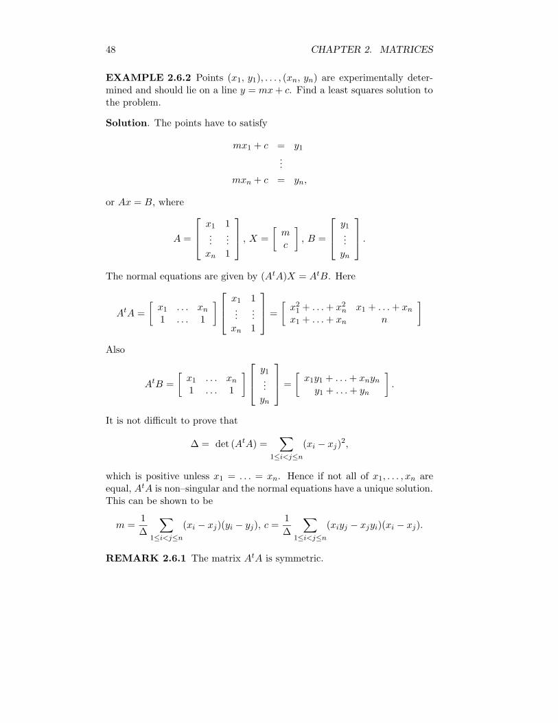
EXAMPLE 2.6.2 Points (x1, y1), . . . , (xn, yn) are experimentally deter-mined and should lie on a line y = mx+ c. Find a least squares solution tothe problem.

Solution. The points have to satisfy

mx1 + c = y1

...

mxn + c = yn,

or Ax = B, where

A =

x1 1...

...xn 1

, X =

[

mc

]

, B =

y1

...yn

.

The normal equations are given by (AtA)X = AtB. Here

AtA =

[

x1 . . . xn

1 . . . 1

]

x1 1...

...xn 1

=

[

x21 + . . .+ x

2n x1 + . . .+ xn

x1 + . . .+ xn n

]

Also

AtB =

[

x1 . . . xn

1 . . . 1

]

y1

...yn

=

[

x1y1 + . . .+ xnyn

y1 + . . .+ yn

]

.

It is not difficult to prove that

∆ = det (AtA) =∑

1≤i<j≤n

(xi − xj)2,

which is positive unless x1 = . . . = xn. Hence if not all of x1, . . . , xn areequal, AtA is non–singular and the normal equations have a unique solution.This can be shown to be

m =1

∆

∑

1≤i<j≤n

(xi − xj)(yi − yj), c =1

∆

∑

1≤i<j≤n

(xiyj − xjyi)(xi − xj).

REMARK 2.6.1 The matrix AtA is symmetric.

2.7. PROBLEMS 49

2.7 PROBLEMS

1. Let A =

[

1 4−3 1

]

. Prove that A is non–singular, find A−1 and


[Answer: A−1 =

[

1

13− 4

133

13

1

13

]

,

A = E21(−3)E2(13)E12(4) is one such decomposition.]

2. A square matrix D = [dij ] is called diagonal if dij = 0 for i 6= j. (Thatis the off–diagonal elements are zero.) Prove that pre–multiplicationof a matrix A by a diagonal matrix D results in matrix DA whoserows are the rows of A multiplied by the respective diagonal elementsof D. State and prove a similar result for post–multiplication by adiagonal matrix.

Let diag (a1, . . . , an) denote the diagonal matrix whose diagonal ele-ments dii are a1, . . . , an, respectively. Show that

diag (a1, . . . , an)diag (b1, . . . , bn) = diag (a1b1, . . . , anbn)

and deduce that if a1 . . . an 6= 0, then diag (a1, . . . , an) is non–singularand

(diag (a1, . . . , an))−1 = diag (a−1

1 , . . . , a−1n ).

Also prove that diag (a1, . . . , an) is singular if ai = 0 for some i.

3. Let A =

0 0 21 2 63 7 9

. Prove that A is non–singular, find A−1 and


[Answers: A−1 =

−12 7 −29

2−3 1

1

20 0

,

A = E12E31(3)E23E3(2)E12(2)E13(24)E23(−9) is one such decompo-sition.]


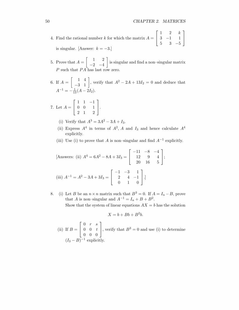
4. Find the rational number k for which the matrix A =

1 2 k3 −1 15 3 −5

is singular. [Answer: k = −3.]

5. Prove that A =

[

1 2−2 −4

]

is singular and find a non–singular matrix

P such that PA has last row zero.

6. If A =

[

1 4−3 1

]

, verify that A2 − 2A + 13I2 = 0 and deduce that

A−1 = − 1

13(A− 2I2).

7. Let A =

1 1 −10 0 12 1 2

.

(i) Verify that A3 = 3A2 − 3A+ I3.(ii) Express A4 in terms of A2, A and I3 and hence calculate A

4

explicitly.

(iii) Use (i) to prove that A is non–singular and find A−1 explicitly.

[Answers: (ii) A4 = 6A2 − 8A+ 3I3 =

−11 −8 −412 9 420 16 5

;

(iii) A−1 = A2 − 3A+ 3I3 =

−1 −3 12 4 −10 1 0

.]

8. (i) Let B be an n×n matrix such that B3 = 0. If A = In−B, provethat A is non–singular and A−1 = In +B +B

2.

Show that the system of linear equations AX = b has the solution

X = b+Bb+B2b.

(ii) If B =

0 r s0 0 t0 0 0

, verify that B3 = 0 and use (i) to determine

(I3 −B)−1 explicitly.

2.7. PROBLEMS 51

[Answer:

1 r s+ rt0 1 t0 0 1

.]

9. Let A be n× n.

(i) If A2 = 0, prove that A is singular.

(ii) If A2 = A and A 6= In, prove that A is singular.

10. Use Question 7 to solve the system of equations

x+ y − z = a

z = b

2x+ y + 2z = c

where a, b, c are given rationals. Check your answer using the Gauss–Jordan algorithm.

[Answer: x = −a− 3b+ c, y = 2a+ 4b− c, z = b.]

11. Determine explicitly the following products of 3 × 3 elementary rowmatrices.

(i) E12E23 (ii) E1(5)E12 (iii) E12(3)E21(−3) (iv) (E1(100))−1

(v) E−112 (vi) (E12(7))

−1 (vii) (E12(7)E31(1))−1.

[Answers: (i)

0 0 11 0 00 1 0

(ii)

0 5 01 0 00 0 1

(iii)

−8 3 0−3 1 00 0 1

(iv)

1

1000 0

0 1 00 0 1

(v)

0 1 01 0 00 0 1

(vi)

1 −7 00 1 00 0 1

(vii)

1 −7 00 1 0

−1 7 1

.]

12. Let A be the following product of 4× 4 elementary row matrices:

A = E3(2)E14E42(3).

Find A and A−1 explicitly.

[Answers: A =

0 3 0 10 1 0 00 0 2 01 0 0 0

, A−1 =

0 0 0 10 1 0 00 0 1

20

1 −3 0 0

.]


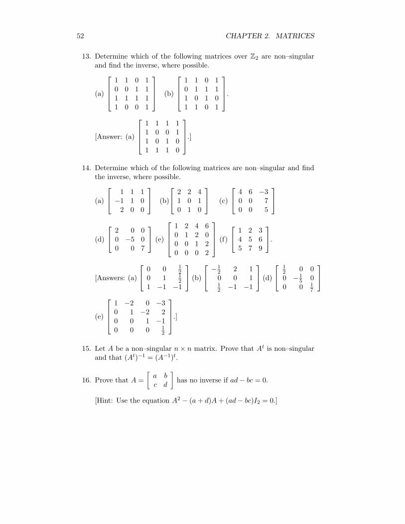
13. Determine which of the following matrices over Z2 are non–singularand find the inverse, where possible.

(a)

1 1 0 10 0 1 11 1 1 11 0 0 1

(b)

1 1 0 10 1 1 11 0 1 01 1 0 1

.

[Answer: (a)

1 1 1 11 0 0 11 0 1 01 1 1 0

.]

14. Determine which of the following matrices are non–singular and findthe inverse, where possible.

(a)

1 1 1−1 1 02 0 0

(b)

2 2 41 0 10 1 0

(c)

4 6 −30 0 70 0 5

(d)

2 0 00 −5 00 0 7

(e)

1 2 4 60 1 2 00 0 1 20 0 0 2

(f)

1 2 34 5 65 7 9

.

[Answers: (a)

0 0 1

2

0 1 1

2

1 −1 −1

(b)

−1

22 1

0 0 11

2−1 −1

(d)

1

20 0

0 −1

50

0 0 1

7

(e)

1 −2 0 −30 1 −2 20 0 1 −10 0 0 1

2

.]

15. Let A be a non–singular n× n matrix. Prove that At is non–singularand that (At)−1 = (A−1)t.

16. Prove that A =

[

a bc d

]

has no inverse if ad− bc = 0.

[Hint: Use the equation A2 − (a+ d)A+ (ad− bc)I2 = 0.]

2.7. PROBLEMS 53

17. Prove that the real matrix A =

1 a b−a 1 c−b −c 1

is non–singular by

proving that A is row–equivalent to I3.

18. If P−1AP = B, prove that P−1AnP = Bn for n ≥ 1.

19. Let A =

[

2

3

1

41

3

3

4

]

, P =

[

1 3−1 4

]

. Verify that P−1AP =

[

5

120

0 1

]

and deduce that

An =1

7

[

3 34 4

]

+1

7

(

5

12

)n [4 −3

−4 3

]

.

20. Let A =

[

a bc d

]

be aMarkovmatrix; that is a matrix whose elements

are non–negative and satisfy a+c = 1 = b+d. Also let P =

[

b 1c −1

]

.

Prove that if A 6= I2 then

(i) P is non–singular and P−1AP =

[

1 00 a+ d− 1

]

,

(ii) An → 1

b+ c

[

b bc c

]

as n→∞, if A 6=[

0 11 0

]

.

21. If X =

1 23 45 6

and Y =

−134

, find XXt, XtX, Y Y t, Y tY .

[Answers:

5 11 1711 25 3917 39 61

,

[

35 4444 56

]

,

1 −3 −4−3 9 12−4 12 16

, 26.]

22. Prove that the system of linear equations

x+ 2y = 4x+ y = 5

3x+ 5y = 12

is inconsistent and find a least squares solution of the system.

[Answer: x = 6, y = −7/6.]


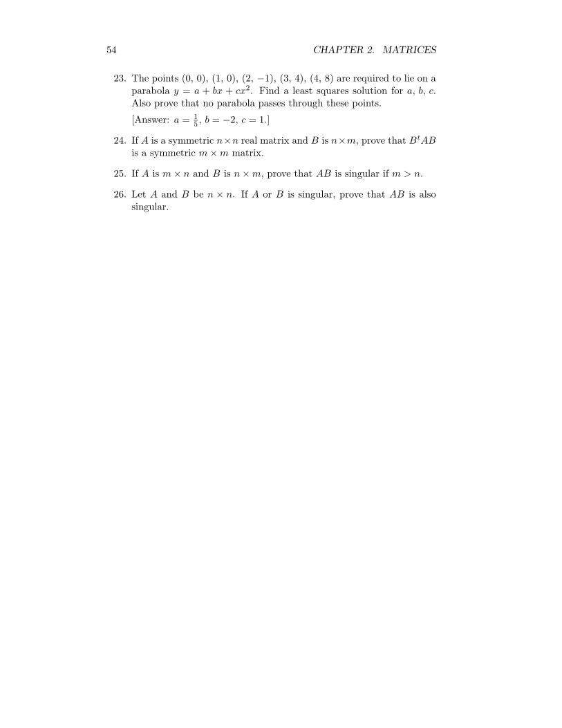
23. The points (0, 0), (1, 0), (2, −1), (3, 4), (4, 8) are required to lie on aparabola y = a + bx + cx2. Find a least squares solution for a, b, c.Also prove that no parabola passes through these points.

[Answer: a = 1

5, b = −2, c = 1.]

24. If A is a symmetric n×n real matrix and B is n×m, prove that BtABis a symmetric m×m matrix.

25. If A is m× n and B is n×m, prove that AB is singular if m > n.

26. Let A and B be n × n. If A or B is singular, prove that AB is alsosingular.

cha2

Documents

aij bij

aij bij

matrix arithmetica matrix

b mmnf

matrix multiplication

b c2

matrix of sizem n

aij meansthat