1

CHAIN STRUCTURE CHARACTERIZATION

Gregory Beaucage and Amit S. Kulkarni Department of Chemical and Materials Engineering, University of Cincinnati, Cincinnati,

Ohio 45221-0012

I. Introduction to Structure in Synthetic Macromolecules

a) Dimensionality and Statistical Descriptions

b) Chain Persistence and the Kuhn Unit

c) Coil Structure and Chain Scaling Transitions

d) Measures of Coil Size Rg and Rh

II. Local Structure and its Ramifications

a) Tacticity

c) Branching

d) Crystallization

e) Hyperbranched Polymers

III. Summary

2

I. Introduction to Structure in Synthetic Macromolecules

a) Dimensionality and Statistical Descriptions

Synthetic polymers display some physical characteristics that we can identify as native to

this class of materials, particularly shear thinning rheology, rubber elasticity, and chain

folded crystals. These properties are inherent to long-chain linear and weakly branched

molecules and are not drastically different across a wide range of chemical make-ups. We

can consider these features to define synthetic macromolecules as a distinct category of

materials. The realization of this special category of materials necessitated the definition of a

structural model broad enough to encompass nylon to polyethylene yet specific enough that

detailed analytically available features could be used to define the major properties of

interest, especially those native to this class of materials. This structural model for polymer

chains is based on the random walk statistics observed by Robert Brown in studies of pollen

grains and explained by Einstein in 1905. It is a trivial exercise to construct a random walk

on a cubic lattice using a PC, Figure 1. From such a walk we can observe certain features of

the general model for a polymer chain. The chain structure differs from conventional

Figure 1. Two examples of Random walks 10,000 steps on a cubic lattice.

structures in that it does not display an obvious surface and incorporates a significant fraction

of solvent within the structure. We can notice 1) The two walks appear different despite

exactly the same algorithm, 2) bunching of steps makes walks seem non-random, in fact

3

bunching is a signature of a random process, 3) One simulation is of no use in describing the

general features of the structure, we must consider a time average or an average over different

structures in space. A classical description of such a structure is of no real use. That is, if we

attempt to describe the structure using the same tools we would use to describe a box or a

sphere we miss the nature of this object. Since the structure is composed of a series of

random steps we expect the features of the structure to be described by statistics and to follow

random statistics. For example, the distribution of the end-to-end distance, R, follows a

Gaussian distribution function if counted over a number of time intervals or over a number of

different structures in space,

!

P R( ) =3

2"# 2

$

% &

'

( )

32

exp *3 R( )

2

2 #( )2

$

% & &

'

( ) ) (1)

This function is symmetric about 0, the starting point as indicated by the symmetric term R2.

Since the distribution is symmetric, the mean value <R> = 0 and we must consider the second

moment as a measure for the size of the structure, <R2>. For a series of n steps of length lK,

where lK is the Kuhn step length, we can consider two contributions to <R2>,

!

R2

=j=1

n

" ri • rj =i=1

n

"j=1

n

" ri • rj +i# j

n

" ri • rii

n

" = nlK2 (2)

where the first term for i ≠ j is 0 since there is no correlation in direction between steps i and j

and the second term yields the result nlK2 since there are n steps where i = j. By considering

that,

!

R2

= R2" P(R)dR =# 2 (3)

we find that the variance, σ2, (square of the standard deviation) for the random walk is given

by (2), nlK2.

4

Polymer chains in dilute and semi-dilute solutions display a statistical structural hierarchy

that differs in essence from the explicit structural hierarchy displayed for example by proteins

in the native state. In proteins the primary residue sequence gives rise to secondary helical

coil and beta sheet structures. These secondary structures compose a complex tertiary

structure and higher order associations of protein chains. For synthetic polymers the

hierarchy begins with the persistence unit that builds upon short-range interactions in a

statistical sense at low chain index difference. Chain persistence can be measured using

viscometry, dynamic light scattering or static scattering measurements. Dynamic

measurements yield directly the Kuhn-length that has been shown to be equivalent to twice

the statically measured persistence length. The Kuhn-length, lK, is the physical step length

for a synthetic polymer chain.

b) Chain Persistence and the Kuhn Unit:

The persistence length, lP, was introduced by Kratky and Porod [1,2,3] as a direct measure

of the average local conformation for a linear polymer chain. The persistence length reflects

the sum of the average projections of all chain segments on a direction described by a given

segment. Kratky [4-6] described the features of the persistence length in a static small-angle

scattering pattern; in particular, a regime of dimension 1 in the small-angle scattering pattern

corresponds to Kratky and Porod’s definition of the persistence unit. The mass-fractal

dimension of an object can be directly determined in a scattering pattern through the

application of a mass-fractal power-law [7]. Using these laws, an object of mass-fractal

dimension df displays a power-law described by, I(q) = Bq-df, for 1 ≤ df < 3. A power-law of -

2 is expected for the Gaussian regime since n ~ R2 and a power-law of -1 for the persistence

regime where the chain appears to be statistically composed of rods. In order to resolve the

persistence length, lP, a log-log plot of I(q) versus q can be made and the two power-law

5

regimes matched with lines of slopes -2 and -1, Figure 2. The intersection of these two lines

in q is related to the persistence length through 6/(πqintersection) = lP (see ref [4], p 363). q is the

absolute value of the momentum transfer vector, q = 4(π/λ) sin(θ/2), λ is the wavelength of

the scattered radiation and θ is the scattering angle. (Equivalently, a “Kratky plot” of Iq2

vs. q

can be made to account for Gaussian scaling, and the deviation from a horizontal line

Figure 2. Kratky/Porod graphical analysis in a log-log plot of corrected SANS data from a 5% by volume d-PHB sample in h-PHB. The lower power -2 line is the best visual estimate; the upper line is shifted to match a global unified fit. Key: left, q* corresponds to best visual estimate; right, plot to match global unified fit. The statistical error in the data is shown [3].

can then be used to estimate lP. This approach has been summarized in several reviews (see

refs [4] and [8] (Appendix G, p 401).

The statistical segment length, lssl, is a related parameter defined as the scaling factor

between the chain’s radius of gyration, Rg, and the square root of the number of chemical mer

units in the chain, nchem, where Rg = 2lssl(nchem/6)1/2

. For a freely-jointed, Gaussian chain,

where the Kuhn unit is a chemical mer unit, 2lssl = lK = 2lP and nK = nchem. The specific

definitions of these terms becomes important for chains with bond restrictions where nK ≠

nchem and 2lssl ≠ lK, that is, the Kuhn segment and the persistence length are both

independently-measurable, physical parameters while, in most cases, the statistical segment

length is an arbitrary parameter which depends on the chemical definition of a chain unit. In

6

general, lK = 2lP as noted above. [9-11] When the global chain scaling deviates from

Gaussian, such as in good and poor solvents, the statistical-segment length refers to an

equivalent-Gaussian chain which does not physically exist. Even under these deviatory

scaling conditions, there remains a scaling relationship between lssl and lK [12], and the

persistence length and Kuhn-step length retain their physical definitions.

Although the definition of the persistence length by Kratky and Porod [1,2] appears to be

somewhat vague in terms of real space, it is the only physical parameter that can be

independently determined that directly reflects local chain conformation at thermodynamic

equilibrium. Because of this, the persistence length is a focus of calculations of chain

conformation using chemical bond lengths and angles [4,8,13]. In the more complicated

chemical structures, seen in biology for instance, such calculations become tedious and are

subject to some degree of uncertainty due to the dominance of secondary chain architecture.

In fact there has been little experimental verification of ab initio calculations of the

persistence length for polymers more complicated than mono-substituted vinyl polymers. The

issue becomes complicated when chain secondary structures such as tacticity and helical

coiling become important to chain conformation [14-19]. A direct measure of the persistence

length using small-angle scattering remains the most robust approach to describing local

chain conformations. A combination of the Kratky-Porod approach with modern scattering

functions and an understanding of fractal scaling laws offer hope in describing both chain

conformation as well as the statistical thermodynamics of these complicated systems. [12]

For a detailed description of the use of small angle scattering to quantify the persistence

length the interested reader is referred to ref. [3].

c) Coil Structure and Chain Scaling Transitions:

As mentioned above, for sizes on the order of the persistence unit the coil size follows the

scaling law,

7

lK~ n1 c (4)

where c is the bond length and n is the number of bonds in a persistence unit. This indicates

that the Kuhn unit [20] is on average a linear structure as can be verified with scattering

measurements where the scattered intensity scales as I(q) ~ q-1 at high-q. At larger sizes and

smaller scattering vector q a different, steeper scaling behavior is observed for synthetic

polymers. This regime reflects the distribution of Kuhn units in space along a curved path

that follows either a self-avoiding or a random walk.

For a self-avoiding walk the coil end-to-end distance, R, scales with,

RSAW ~ n3/5 lK (5)

where n is the number of Kuhn units of length lK. If self-avoidance is removed by screening

of excluded volume the coil can take a Gaussian configuration where the coil size scales with,

RGaussian ~ n1/2 lK (6)

Equation (6) is the result of a calculation of the root mean square end to end distance from

the summation of equation (2). Equation (5) cannot be obtained by such a direct calculation

since it involves non-random chain scaling due to long-range interactions. Equation (5) is

obtained by considering a comparison between equation (1) and the Boltzman distribution

function for a system at thermal equilibrium,

!

PBR( ) = exp "

E R( )kT

#

$ %

&

' ( (7)

which yields a function for the free energy of the Gaussian chain,

!

E = kT3R

2

2nlK

2 (8)

8

For a chain with excluded volume the probability of the chain avoiding one segment of

volume Vc is PEx(R) = 1 - Vc/R3. The total number of combinations of two chain units is n(n-

1)/2! ~ n2/2 so the total probability of exclusion is,

!

PExR( ) = 1"V

cR3( )

n2

2 = expn2 ln 1"V

cR3( )

2

#

$ % %

&

' ( ( ~ exp "

n2Vc

2R3

#

$ %

&

' ( (9)

Through multiplication of this probability with the Gaussian function equation (1), and by

comparison with equation (7),

!

E = kT3R

2

2nlK

2+n2Vc

2R3

"

# $

%

& ' (10)

Equation (10) yields decidedly non-Gaussian behavior and the chain end-to-end distance

probability function using (10) in (7) can not be analytically integrated for moments such as

the RMS end-to-end distance. For this reason a different approach is used to define a

preferred chain size for the self-avoiding walk using a derivative rather than an integral. A

probability function proportional to the probability of a chain starting at radius of 0 having an

end in a spherical shell of a radius R from the center,

!

W (R)dR = kR2exp "

3R2

2nlK

2"n2Vc

2R3

#

$ %

&

' ( dR (11)

This function displays a maximum at the preferred chain end to end distance R* that can be

found by setting the first derivative to 0,

!

R*

R0

*

"

# $

%

& '

5

(R*

R0

*

"

# $

%

& '

3

=9 6

16

Vc

lK

3n (12)

where R0* is the maximum probability for the Gaussian function,

9

!

R0

*=2nl

K

2

3

"

# $

%

& '

1 2

(13)

(12) can be simplified by considering large R*/R0* so that

!

R*

R0

*

"

# $

%

& '

5

>>R*

R0

*

"

# $

%

& '

3

to yield the scaling

relationship,

R* ~ lK n3/5 (14)

which is the expression for a self-avoiding walk (SAW).

Vc in equation (10) represents a hard-core repulsion that is entropic in nature since it is

linearly dependent on temperature in the expression for energy, (10). Repulsion is generally

associated with enthalpic interactions and we can consider the effect of an enthalpic

interaction. Since Vc is associated with a single Kuhn unit we consider the average enthalpy

of interaction per pair-wise interaction and the number of pair-wise interactions per Kuhn

unit,

!

"# = #PP

+ #SS( ) 2 $#PS (15)

where εPP is the average polymer-polymer pair-wise interaction energy, εSS is the average

solvent-solvent pair-wise interaction energy and εPS is the average pair-wise interaction

energy for polymer-solvent. Each Kuhn unit has z pair-wise interactions where z is the

coordination number (on a cubic lattice for instance). In order to remove the kT dependence

introduced by (10) we write,

!

" =z#$

kT (16)

and

10

!

Vc,enthalpic =Vc 1" 2#( ) (17)

where the factor 2 is included since there is no redundancy in interactions in equations (15)

and (16) when used in equation (10). The free energy for an isolated chain with enthalpic

interactions can be written,

!

E = kT3R

2

2nlK

2+n2Vc1" 2#( )2R

3

$

% &

'

( ) (18)

Equations (18) and (16) define a temperature where Gaussian behavior is observed (the phase

separation temperature) where χ = ½ and thermal energy is just sufficient to break apart PP

and SS interactions to form PS interactions. Equation (12) using (17) for Vc is called the

Flory-Krigbaum equation. This expression indicates that only three states are possible for a

polymer coil at thermal equilibrium: 1) The normal condition in solution reflected by a self-

avoiding walk, 2) A unique condition seen exactly at the phase separation temperature

reflected by Gaussian scaling, and 3) The collapsed state at temperatures below the phase

separation temperature for a UCST system. For a chain at equilibrium no other states are

possible!

The SAW, (14) and (18), is the normal condition for a polymer chain in solution and this

can be easily verified by observation of the fractal scaling regime in neutron scattering

measurements. Polymers generally have limited solubility and it is often possible to bring a

polymer solution to the phase separation point thermally, either by cooling (polystyrene in

cyclohexane) or by heating (polyvinylmethylether in water). It has been found

experimentally that chain scaling just at the phase separation temperature follows the

Gaussian prediction of equation (2).

11

Figure 3. Radius of gyration, Rg, and hydrodyamic radius Rh versus temperature for polystyrene in cyclohexane. Vertical line indicates the phase separation temperature. From Reference [21].

However, it is known that the overall coil size varies with temperature which indicates that

the 3-state model is incomplete. It is possible to resolve the apparent discrepancy between an

expanding coil size and fixed chain scaling by considering a size dependent thermodynamics

within the coil. This is possible for high polymers because the energy expression in equation

(18) depends on coil size through n. For example, the energy of a chain calculated using (18)

is different for a chain of 500 Kuhn units compared to a chain of 1000 Kuhn units. However,

a chain of 1000 Kuhn units is composed of 2 chains of 500 units and many chains of smaller

sizes. Smaller chains have less entropy from (18) and would be expected to thermally phase

separate first. For example as temperature is dropped towards the phase separation

temperature in a UCST system we observe that the coil decreases in size. The coil at the

small sizes reaches a point of phase separation at a higher temperature than the coil at large

sizes. Locally we observe 3 regimes of scaling, linear persistence at smallest sizes, Gaussian

at intermediate sizes where there is insufficient entropy for miscibility and expanded coil

SAW at large sizes where there is sufficient entropy for miscibility. The size-scale for

transition between the latter two sizes is termed the thermal (or thermic) blob. Coils can

12

show a gradual change in size with cooling due to changes in this thermal blob size. The

chain also follows only the 3 possible states (Gaussian, SAW or collapsed). Once the entire

coil has reached the miscibility limit the chain finally phase separates just after displaying

true Gaussian scaling on cooling for a UCST system. The thermal blob has been verified

using small-angle neutron scattering [142]. The understanding that polymers display an

ability to accommodate thermal changes through scaling transitions was a major development

in theoretical physics with ramifications to other chain and network structures such as

proteins, DNA and elastomers.

Similar scaling transitions on external perturbation are known for stress, tensile blob, and

concentration, concentration blob, as well as other possible chain perturbations.

Concentration is of particular importance since it allows an understanding of the progression

from a good solvent to the melt with increasing concentration. This progression is also of a

gradual type despite the required 3 discrete state prediction and we explore the possibility of

a scaling transition within the coil to explain this behavior. In progressing from a dilute

solution to a concentrated and to the melt state we expect miscibility to decrease and the coil

to contract. For a coil in dilute solution the coil displays two sizes, the overall coil size or

end to end distance and the Kuhn length. As concentration increases a point is reached where

the concentration within a coil, n/R3, is matched by the solution,

c* = k n/R3 = k n-4/5 (19)

where the latter expression relied on (14). At this point coil overlap occurs and we do not

expect thermodynamic parameters to depend on the overall coil size but on a new size

introduced due to the increasing concentration. We can consider a scaling transition to occur

at a size scale ξ associated with the overall coil size R and the reduced concentration,

13

ξ ~ R (c/c*)P ~ n(3+4P)/5 (20)

The last equality is obtained by considering (19). Since we know that the scaling transition

size is not dependent on n above c*, then P = -3/4 and,

ξ ~ R (c/c*)-3/4 (21)

This concentration dependent scaling transition is known as the concentration blob. At large

size scales the coil displays Gaussian scaling while at small size scales the coil displays SAW

scaling since the coil at sizes larger than the scaling transition exist in a melt like state where

interactions are screened. At the transition size SAW scaling is obeyed ξ = lK nξ3/5, so with

(21), nξ is equal to (c/c*)5/4, and with Gaussian scaling at large size scales,

R = ξ nξ1/2 = RF0 (c/c*)-3/4 (c/c*)5/8 = RF0 (c/c*)-1/8 (22)

Equation (22) has been confirmed by a variety of techniques including neutron scattering,

dynamic light scattering and osmotic pressured measurements [143]. As concentration

increases the concentration blob decreases in size until the Kuhn length is reached and the

coil displays concentrated or melt Gaussian structure. The coil accommodates concentrations

between the overlap and concentrated through adjustment of the concentration blob size.

A similar scaling transition has been proposed to account for the response of an isolated

coil to tensile stress [144,145]. If a force is applied to a Gaussian coil (8) can be used to

calculate the response of the coil since at thermal equilibrium the applied force F ~ dE/dR so,

!

F =dE

dR=3kT

nlK

2R (23)

14

which defines the spring constant for an isolated coil. For weak perturbations the end to end

distance R is close to n1/2lK so F ~ 3kT/Rt, where Rt is the tensile blob size. This can be

rearranged to express a size dependent on the applied force,

!

Rt

=3kT

F (24)

Rt decreases in size for larger applied forces. Equation (24) describes a size scale governed

by a balance between the thermal energy of the coil and the applied force. For sizes larger

than this scaling transition the coil presents no resistance to the applied force and we expect a

linear structure with R ~ nt Rt. For sizes smaller than this scaling transition we expect to

observe the native scaling of the chain either Gaussian or SAW scaling. A similar behavior

can be observed when straightening a kinked string, that is large scales straighten out earlier

with increasing applied force compared to smaller features.

For the tensile blob, thermal blob and concentration blob we find that the coil

accommodates external stress (thermal, concentration or force) through a scaling transition

that leads to two regimes of chain scaling. This directly impacts the free energy of the chain,

the mechanical response and the coil size.

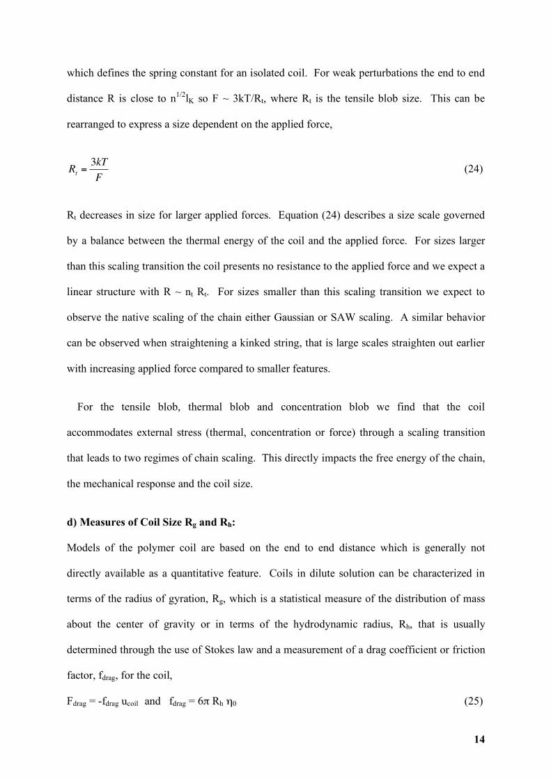
d) Measures of Coil Size Rg and Rh:

Models of the polymer coil are based on the end to end distance which is generally not

directly available as a quantitative feature. Coils in dilute solution can be characterized in

terms of the radius of gyration, Rg, which is a statistical measure of the distribution of mass

about the center of gravity or in terms of the hydrodynamic radius, Rh, that is usually

determined through the use of Stokes law and a measurement of a drag coefficient or friction

factor, fdrag, for the coil,

Fdrag = -fdrag ucoil and fdrag = 6π Rh η0 (25)

15

where ucoil is the velocity of the coil, η0 is the viscosity of the pure solvent and Fdrag is the

force associated with drag of a moving coil in a solvent. Under the assumption that the coil is

non-draining (Kirkwood Reisman theory), Rh reflects the radius of a sphere enclosing the

coil. There is no clear means to verify the non-draining assumption and generally Rh should

be considered a value that scales with the end to end distance. The radius of gyration, on the

other hand, has an analytic relationship to the coil end to end distance.

Rg2 is expressed as,

!

Rg

2 =1

nri " RG( )

2

i=1

n

# (26)

where RG is the center of mass,

!

RG =1

nri

j=1

n

" (27)

Combining (26) and (27) yields,

!

Rg

2 =1

2n2

ri " rj( )2

j=1

n

#i=1

n

# =1

2n2

i " jj=1

n

#i=1

n

# lK2 =

1

n2

i " j( )j=1

n

#i= j

n

# lK2

=lK

2

n2z + 2 z "1( ) + 3 z " 2( )K z "1( )2 + z[ ]

(28)

where z = n - 1. The last series can be obtained by constructing an n by n matrix of i versus j

with values of |i - j| and recognizing that the matrix is symmetric about i = j. The bracketed

expression in (28) can be rewritten,

!

z +1" p( )p = z +1( )p=1

z

# pp=1

z

# " p2

p=1

z

# =z z +1( ) z + 2( )

6$n3

6 (29)

using

16

!

up

u=1

N

" =N

p+1

p +1+N

p

2+pn

p#1

12 for p < 3 (30)

Using (29) in (28),

!

Rg

2=nlK2

6=

R2

6 (31)

(31) applies to monodisperse systems. For polydisperse systems Rg2 reflects a high order

moment of the distribution, the ratio of the 8’th to the 6’th moment of the distribution in

mean size. For this reason Rg will correlate with the largest sizes of a distribution. There are

several advantages to Rg as a measure of size over the end to end distance. For branched, star

and ring structures the end to end distance has no clear meaning while Rg retains its meaning.

Further, Rg is directly measured in static scattering measurements so it maintains a direct link

to experiment.

II. Local Structure and its Ramifications

a) Tacticity:

Local chain structure is governed by chemical make-up, configuration and

conformation. Polymer chain conformation refers to the different orientations of the repeat

units brought about by bond rotations. Configuration on the other hand cannot be changed by

simple bond rotations, and refers to how the units add into the polymer sequentially during

polymerization. An example of different polymer chain configurations is that brought about

by head-to-head addition of repeat units as opposed to head-to-tail addition. In the case of

vinyl polymers (-CHX-CH2-) the substituted carbon is usually designated as the head, and the

unsubstituted methylene unit is designated as the tail.

Tacticity in Polymers: Polymers formed from substituted monomers, like vinyl

polymers, display tacticity which has bearing on the final polymer properties like degree of

17

crystallinity, crystalline phase structure and melting temperatures as well as glass transition

temperature for di-substituted vinyl polymers. Tacticity or handedness describes the

stereochemical arrangement of a chain unit relative to other chain units. The smallest unit of

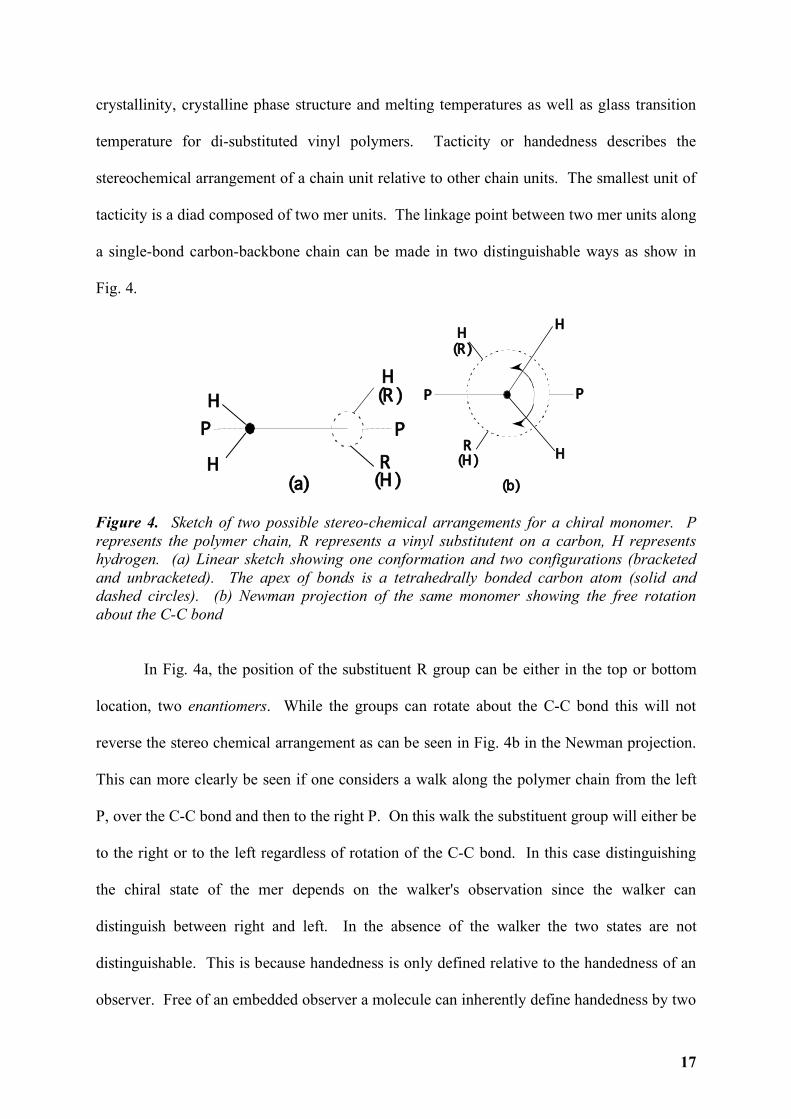
tacticity is a diad composed of two mer units. The linkage point between two mer units along

a single-bond carbon-backbone chain can be made in two distinguishable ways as show in

Fig. 4.

PP

(R)

(H)H

H

H

R

(a)

PP

(H)

H

H

(R)H

R

(b)

Figure 4. Sketch of two possible stereo-chemical arrangements for a chiral monomer. P represents the polymer chain, R represents a vinyl substitutent on a carbon, H represents hydrogen. (a) Linear sketch showing one conformation and two configurations (bracketed and unbracketed). The apex of bonds is a tetrahedrally bonded carbon atom (solid and dashed circles). (b) Newman projection of the same monomer showing the free rotation about the C-C bond

In Fig. 4a, the position of the substituent R group can be either in the top or bottom

location, two enantiomers. While the groups can rotate about the C-C bond this will not

reverse the stereo chemical arrangement as can be seen in Fig. 4b in the Newman projection.

This can more clearly be seen if one considers a walk along the polymer chain from the left

P, over the C-C bond and then to the right P. On this walk the substituent group will either be

to the right or to the left regardless of rotation of the C-C bond. In this case distinguishing

the chiral state of the mer depends on the walker's observation since the walker can

distinguish between right and left. In the absence of the walker the two states are not

distinguishable. This is because handedness is only defined relative to the handedness of an

observer. Free of an embedded observer a molecule can inherently define handedness by two

18

neighboring chiral centers. For two chiral centers along a polymer chain a diad can identify

two states, similar enantiomers or a meso diad (m) and dissimilar enantiomers or a racemic

diad (r). In a meso diad a walker along the chain would find substituent groups both on the

right side, for example, in the walk described above. There are two possible arrangements of

meso diads (left-left or right-right) and two possible arrangements of racemic diads (right-left

or left-right) so that an unbiased stereochemical arrangement would contain 50% meso diads.

This could be one description of an atactic or non-tactic polymer. However, few properties

of polymers are associated with diad tacticity since most properties are associated with longer

groupings of mer units. For example, the stereochemistry of diads has little direct effect on

the ability of long sequences of a chain to form a helix and to crystallize. Finally, there is no

quantitative analytic technique to directly measure diad tacticity in polymers. The smallest

unit that can be observed, by NMR for instance, requires groupings of three mer units. This

is because NMR relies on splitting of absorption peaks associated with the distinguishing

different neighboring chiral groups. For a given mer unit two neighboring mer units can be

equally observed leading to a group of 3 mer units. This triad can have one of three

arrangements, mm (isotactic), rr (syndiotactic) or mr/rm (heterotactic). Since there are twice

as many possible arrangements of heterotactic, a random mixture of triads would result in

25% isotactic triads, 25% syndiotactic and 50% heterotactic triads. This could be an

alternative definition of an atactic polymer. It should be noted that a polymer defined as

atactic by diads could be 100% heterotactic or could have many other stereochemical

arrangements of triads. Then there is a limited connection between tacticities as measured at

different orders in going from low order to higher order (diads to triads). We can use

statistics to predict the most likely triad arrangement associated with a given diad

distribution. Higher order tacticities are associated with only one lower order distribution.

Generally we are interested in the highest possible order of tacticity since this governs

19

properties of a macromolecule. High order stereochemical arrangements do not have names

associated with their states since a plethora of arrangements are possible. Generally, we

speak of odd orders, 3 (triad), 5 (pentad), 7 (heptad) etc. due to the nature of the NMR

measurement mentioned above.

Determination of tacticity (stereoregularity)

The tacticity or distribution of asymmetric units in a polymer chain can be directly

determined using nuclear magnetic resonance spectroscopy (NMR) and infra red

spectroscopy and has been studied for a variety of polymers. Fig. 5a and b shows the proton

NMR spectra [22, 23] and IR spectra [24, 25] respectively for the two stereoisomers of

polymethylmethacrylate (PMMA), syndiotactic and isotactic PMMA. These two structures in

a polymer like PMMA give rise to different signatures in both the techniques. In case of the

NMR spectra [22, 23], the occurrence of a peak at 8.78 ppm chemical shift (tetramethylsilane

peak at 10.00 ppm) as seen in the lower spectrum of Fig. 5a corresponds to the meso

placement of the alpha methyl units and hence represents isotactic PMMA spectrum. The

upper spectrum in Fig. 5a [22, 23] with a peak at chemical shift of 9.09 ppm corresponds to

the racemic placement of the alpha methyl units and hence a syndiotactic PMMA spectrum.

The sensitivity of the chemical shift of the alpha methyl protons is accepted to be a

fundamental feature reflecting the stereochemical configuration of PMMA. These specific

shifts arise from triad sequences in PMMA. Higher order sequences can be detected in

different polymers by going to higher magnetic fields. From the IR spectra shown in Fig. 5b

[24, 25], peak assignments can be made for the two configurational isomers of PMMA and

are given in Table I. Some basic aspects of the selection rules for infra red spectroscopy and

Raman scattering for the detection and characterization of stereoregularity for such polymers

are given in ref [26].

20

Figure 5. a) Proton NMR spectra [22, 23] for syndiotactic (upper) and isotactic (lower) polymethylmethacrylate b) IR spectra [24, 25] for syndiotactic and isotactic polymethylemethacrylate.

Table I. IR peak assignments for isotactic and syndiotactic polymethylmethacrylate [24].

Isotactic Syndiotactic Peak Assignment

1465 1450 δ(CH2), δa(CH3-O)

1190 1190 Skeletal

996 998 γr(CH3-O)

950 967 γr(α-CH3)

759 749 γ(CH3) and skeletal

Similar studies have been conducted on polyvinylchloride (PVC) to assign different IR

signatures obtained from different stereo-configurational isomers. The sensitivity of the C-Cl

bond on the stereochemical environment has been utilized using IR spectroscopy. The

characteristic vibrations of the C-Cl bonds are inherently tied in to the configuration as well

as the conformation of the polymer. The effects of configuration and conformation on the IR

peak assignments for PVC are given in Table II [25, 27].

a) b)

21

Table II. IR peak assignments for polyvinyl chloride based on polymer conformation and configuration [27]. Peak (cm-1) Conformational Assignment Configuration

602 TTTT long sequences Syndiotactic

619 TTT short sequences Syndiotactic

639 TTTT long sequences Syndiotactic

651 TTTG syndiotactic Syndiotactic

676 TG*G* syndiotactic Syndiotactic

697 TGTG isotactic Isotactic

The commercialization of polypropylene (PP) had been revitalized with the advent of

metallocene and vanadium based catalyst systems which result in highly stereo-regular

isotactic and syndiotactic PP respectively [28]. The advent of these catalyst systems has

enabled the synthesis of these PP isomers with enhanced physical properties [29] and

applications [30]. Recently Rojo et al. [28] have devised a rheology based technique to

differentiate between streo-isomers of polypropylene. The procedure involves plotting the

loss tangent (δ) as a function of the complex modulus G* as shown in Fig. 6 [28].

Differentiating between syndiotactic and isotactic PP’s is based on the higher values of

Newtonian viscosities, terminal relaxation times, and activation energies for flow for

syndiotactic PP samples [28]. Positive identification and differentiation of isomers is possible

by plots like the one shown in Fig. 6, plots of loss tangent values versus complex modulus

[28].

22

Figure 6. Loss tangent (δ) plotted as a function of complex modulus G* for a series of syndiotactic and isotactic polypropylene from the work of Rojo et al. [28].

A consequence of tacticity/stereoregularity is the production of regular helical coiling

of the polymer chain. Helical coiling is a secondary structure for synthetic polymers

associated with the primary structure of the tactic sequence. Using IR spectroscopy, it has

been possible to assign some unique bands to tacticity in polymers with helical chain

structure. These bands are classified as the helix bands and regularity bands [26]. The helix

band not only depends on the nature of tacticity, but on the sequence length of the stereo-

configuration. Thus additional microstructural information can be obtained from such IR

studies. The values of such absorption bands for some common polymers like polypropylene

and polystyrene can be readily found in texts on this subject [26].

c) Branching:

The presence of branches along the main chain of a polymer molecule significantly alters the

static and dynamic properties of the polymer [31]. The presence of structural branching is not

23

limited to commercial polymeric materials like polyolefins, but plays an important role in

altering the properties of a broad spectrum of materials which can be classified as nano-

particulate ceramic aggregates, polymeric networks and gels. Branch content and nature, has

a strong influence over structure-property relationships of these materials. For example, the

presence of branch content dictates the crystallization behavior [31] of commercial

polyolefins and copolymers, the mechanical properties of cross-linked macromolecules, and

the nature and extent of reinforcement obtained from aggregated inorganic materials like

silica and titania [32-37] when dispersed in an organic polymeric matrix. The need of

quantifying branch content in such materials is of vital significance not only to predict the

structure-property relationships dictating characteristic material performance in end-

applications, but also to gain a better understanding of the underlying thermodynamic and

kinetic processes [38-48] governing the synthesis of these materials. Estimating branch

content through the development of novel analytical approaches has been a quest for

materials scientists for well over five decades.

One of the very first approaches to estimate branch content in polymers was using

size exclusion chromatography (SEC). The solution properties of a branched polymer

molecule differ vastly from that of its linear analogue. The vital difference between a

branched and a linear polymer molecule is in the size that they exhibit in solution. Size

exclusion chromatography essentially fractionates a polydisperse polymer sample into

monodisperse-fractions based on their molecular size in solution. Hence estimating branch

content for polydisperse polymers from SEC is based on this disparity of molecular sizes of

branched and linear polymer molecules. Nuclear magnetic resonance spectroscopy has been a

very effective tool to estimate branch content in polymers on a quantitative basis. It has the

added advantage of being able to discern the branch lengths up to a certain degree. C-13

NMR spectroscopy has been mostly used to carry out such an analysis and depends on the

24

calculations of the chemical shifts arising due to the presence of structural branching.

Favorable rheological properties are an essential requirement for the commercialization of

polyolefins like polyethylene. The ease of processability of the polymer melt, obtained

through modifications in the micro-structural features is as important as the end-use

mechanical properties of these polymers. Presence of long chain as well as short chain

branching more or less dictates the rheological behavior of most commercial polyolefins.

Inherently, various studies have been conducted over the years linking the melt behavior to

the underlying polymer chain micro-structure. As already stated, apart from the importance of

estimating branch content for determining structure-property relationships, the quest to

ascertain the branch content information also has some motivation to for enhancing our

understanding of some fundamental phenomenon, e.g. phase separation [38-47] between

polyolefins blends of high density polyethylene and linear low density polyethylenes has

been reported in literature, where the amount of branches in the linear low density material

govern the occurrence of micro-phase separation. Similarly, even cross-linked materials like

poly(dimethylsiloxane) (PDMS) [48] exhibit phase separation driven by a disparity in the

topological features of the two phases. The presence of short chain branching and its

estimation has been fundamental to discerning the crystallization kinetics and mechanisms in

commercial polyolefins like ethylene-alkene copolymers.

Types of Branching in Polymers: The nature and amount of branch content in

macromolecular systems is diverse and plays a fundamental role in their characteristic

behavior [49-53]. Apart from molecular weight and molecular weight distributions, the nature

of branching leading to different topological features can be considered as one the most

fundamental features dictating the properties of macromolecules. The classification of many

systems is based on the nature of their topological features. Branching in commercial

25

polyolefins is classified as long chain or short chain branching. The presence of either long or

short chain branching has unique effect on the properties of these polymers. Long chain

branched polymers are usually classified to be described as randomly branched polymers.

Short chain branching in polymers leads to structures usually defined as ladder-architecture.

Graft-copolymers, where short branches of one polymer are present on the backbone of a

second polymer are a special case of ladder polymers. Multi-arm star polymers have also

been extensively studied for their unique properties. Dendrimers and hyperbranched

polymers represent another class of highly branched polymers. Hyperbranched polymers are

similar in structure to dendrimers, but lack a central core from which growth occurs through

hierarchical levels as in dendrimers, and are usually synthesized in a one step process. The

schematic representation of these various branched architectures is shown in Fig. 7.

Figure 7. Schematic representation of different types of branched structures as discussed in the text. The crystallization kinetics of commercial polyolefins is to a large extent determined

by the chain micro-structure [54-56]. The kinetics and the regime [56] of the crystallization

26

process determine not only the crystalline content, but also the structure of the interfaces of

the polymer crystals. This has a direct bearing on the mechanical properties like the modulus,

toughness and other end use properties of the polymer in fabricated items like impact

resistance and tear resistance. Such structure property relationships are particularly important

for polymers with high commercial importance in terms of the shear tonnage of polymer

produced globally, like polyethylene and polyethylene based co-polymers. It is seen that in

the case of linear low density polyethylene, which is essentially a copolymer of ethylene and

1-alkenes like hexene and octene, giving rise to butyl and hexyl branches on a polyethylene

backbone, apart from the amount of 1-alkene comonomer, branch content, and small-chain

branch length, the primary modulator controlling the crystallization behavior is the sequence

length distribution arising from these short chain branches [54, 55, 57]. Hence, characterizing

the sequence length distribution using spectroscopic techniques is as important as quantifying

the short chain branch content.

Hyperbranched polymers (HBP’s) [58-60] represent a special class of polymers with

unique set of properties. The development of synthesis chemistries of such materials has been

fueled by the numerous potential applications such materials are expected to have.

Characterization of the chain structure of such topologically unique materials is critical to

understanding and predicting their properties.

Size Exclusion Chromatography

SEC (also known as gel permeation chromatography) is routinely used to characterize the

molecular weight distribution in a polydisperse polymer sample. Fractions with different

molecular weights are separated by passing a solution of the polymer through a series of

columns on the basis of their hydrodynamic volume [61-64], which is the product of the

intrinsic viscosity (limiting viscosity, [η]) and the viscosity average molecular weight Mv.

The universal calibration curve, obtained from standard polymer samples of known molecular

27

weight distribution is used to compare with the elution profile for the given polymer sample.

Most modern SEC setups are equipped with a triple detection system. They consist of an

inline viscometer detector (VD), a refractive index detector (RID), and a light scattering

detector (LS). The VD can be used to continuously monitor the intrinsic viscosity [62, 63] of

the eluting fractions, with the concentration of the given fractions being ascertained by using

the RID.

Though SEC is used to characterize the molecular weight distribution in a polymer

sample, it separates a polydisperse polymer sample on the basis of the hydrodynamic size of

different fractions and not their molecular weights [62, 63]. Hence a branched polymer

molecule and a linear polymer molecule of equal size cannot be differentiated by a SEC

technique, since both of these would elute out at time same time. For a branched polymer

molecule and its linear analogue (having the same molecular weight as the branched

molecule) the radius of gyration of the linear polymer will be greater [62] than that of the

branched molecule, as can be seen in the schematic shown in Fig. 8.

Figure 8. Difference in the size of a branched polymer molecule (b) compared to its linear analogue (a) of the same molecular weight in solution.

In their seminal work in 1949, Zimm and Stockmayer [65] defined the ratio of the mean

square radii of gyration of a branched and a linear polymer of equal molecular weight as the

parameter g and is related to the parameter g’, which is the ratio of the intrinsic viscosities of

a branched and a linear polymer [61-65]

28

[ ][ ]l

b

lg

bg

e

gandR

Rgwhere

gg

!

!==

=

';,2

2

'

(32)

where e is a scaling constant, <Rg2> is the mean square radius of gyration, [η] is the intrinsic

viscosity, and the subscripts b and l refer to the branched and linear polymer. The intrinsic

viscosity and molecular weight measured in a SEC experiment correspond to the actual

branched molecule being run through the column. The Mark-Houwink equation can be used

to calculate the intrinsic viscosity of the linear analogue with the same molecular weight as

the branched polymer being run through the SEC and is given by,

[ ] a

lKM=! (33)

where K and a are constants for a given polymer-solvent pair. This analytical procedure

results in the estimation of the parameter g. The Zimm-Stockmayer relationship (eq. 34 [65])

is used to estimate the branch content. The Zimm-Stockmayer relationship is specific to the

nature of branch content. It requires a prior knowledge of the functionality of the branch point

in the main chain, as well as the dispersion in the branch lengths (whether the branch lengths

are monodisperse or random) [62-64]. For polydisperse branch lengths with tri-functional

branch points, g is given as [62-65],

( )

( )

( ) ( )

( ) ( ) !"

!#$

!%

!&'

((+

+++= 1

2

2ln

221

6

2/12/1

2/12/1

2/1

2/1

3

ww

ww

w

w

w

wnn

nn

n

n

ng (34)

where the subscripts 3 and w indicate tri-functional branch points with polydisperse branch

lengths and nw is the weight average number of branches per molecule. The parameter nw then

needs to be converted to express branch content in conventional terms of number of branches

per 1000 backbone carbon atoms, and is given as [63] (for polyethylene),

)14000(1000 M

n

C

LCBw= (35)

29

where M is the molecular weight, and 14000 corresponds to the molecular weight of 1000

repeat units of a -(CH2)- molecule.

Inspite of the analytical nature of SEC to estimate branch content in polymers, it represents a

relative/secondary technique to based on indirect calculations of iterative solutions of eq. 32

and eq. 34 [64]. There is a disparity in the experimental conditions and the theoretical

assumptions involved in estimating branch content. SEC experiments are carried out in good

solvents (good solvent scaling for the polymer molecules) whereas the Zimm-Stockmeyer

relationships were derived for theta solution conditions (e = 1/2) which imply a Gaussian

scaling. The effect of these assumptions on different branched polymer systems cannot be

estimated. The sensitivity of the detectors used in a SEC experiment dictate the accuracy of

the obtained results (Fig. 9). Molecular weight sensitive detectors like viscometer detectors

(VD) and light scattering detectors (LS) show poor response in the low molecular weight tail

of the chromatogram, whereas concentration sensitive detectors like differential refractive

index detectors (DRI) have a poor response in the high-molecular weight slice of the raw data

[66]. Multi-detector configurations (triple detector) seem to have overcome some of these

difficulties; though it has lead to an increased complexity in the experimental procedures. The

disparity in the intrinsic viscosity of a branched polymer compared to a linear analogue is

used to estimate branch content by using SEC. The presence of short chain branching does

not significantly alter the intrinsic viscosity of a polymer molecule. The reduction in [η] due

to short chain branching is estimated to be only 0.01 times [62] that due to long chain

branches. Hence the sensitivity of SEC to estimate short chain branching is limited, and only

high levels of long chain branching can be estimated effectively, where comparative data is

lacking as discussed below in the section concerning nuclear magnetic resonance

spectroscopy.

30

Figure 9. Response versus retention volume for a) RID, b) VD and c) LS detector for the same sample [66].

Nuclear Magnetic Resonance Spectroscopy

Nuclear magnetic resonance spectroscopy (NMR) can be utilized to obtain branch content

information for commercial polymers in a direct quantitative manner. Polyethylene and

polyvinylchloride are the two commercial polymers that have been studied exhaustively for

branch content determination by this technique [67-71]. Obtaining branch content

information from such polymers has been dealt with, by using high resolution 13C-NMR. This

technique involves assignment of the specific shifts in the radio frequency vibrations arising

due to a branch point in a carbon backbone chain. Conventionally, these radio-frequency

shifts have been calculated for up to 5 carbon atoms from the branch point [72]. Such an

analysis results in the direct estimation of the branching density in the polymer sample like

polyethylene. In the case of polyvinylchloride, the approach is not as simple as in the case of

polyethylene, with complications arising due to the stereochemical isomerization in structure

31

due to the presence of the chlorine side groups along the main chain [66]. This necessitates

the removal of the chlorine atoms via a reductive de-chlorination process using either lithium

aluminum hydride [73] or tri-butyl tin hydride [74]. Once the de-chlorination step is

complete, branch content in polyvinylchloride can be obtained similar to polyethylene using

high resolution 13C- NMR spectroscopy. The technique of obtaining the shifts in the radio-

frequency vibrations due to branch points was developed by Grant and Paul [75] and shall be

briefly discussed below.

Grant and Paul Chemical Shifts:

The technique of obtaining branch content information from NMR for polymers utilizes an

empirical relationship given by Grant and Paul [75]. The Grant and Paul empirical

relationship [75] can be used to calculate the values of the chemical shifts for carbon atoms in

the vicinity of a branch point in a hydrocarbon polymer. The empirical relationship was

obtained from NMR studies on alkanes. The chemical shift of any carbon atom in a 13C-NMR

can be decomposed as a sum of contributions from its nearest 5 neighboring carbon atoms.

The value of the chemical shift for any carbon atom *C, is given as,

( ) CShiftChemical +++++= !"#$%2 (36)

where α, β, γ, δ, and ε are called Grant and Paul parameters, and C is a constant, the values

are outlined in Table III [75].

32

Table III. Grant and Paul parameters obtained from alkanes [75].

Grant & Paul

Parameters Shift (ppm)

Α 8.61

β 9.78

γ -2.88

δ 0.37

ε 0.06

C -1.87

This empirical relationship cannot be used with accounting for some correction terms which

take into account the molecular geometry of the bonded neighbors. This is especially

essential when calculating the chemical shift of a branch point carbon atom. These correction

terms were given by Grant and Paul to be as follows [75],

TABLE IV. Correction values for branched polymers [75].

Shift (ppm)

3o(2o) -2.65

2o(3 o) -2.45

1o(3o) -1.40

where, 3o, 2o, and 1o represent tertiary, secondary and primary carbon atom (Fig. 10), and

3o(2o) represents correction for a tertiary carbon bonded to a secondary, as in a methine group

to a methylene. In a study conducted by Randall [76], the temperature dependence of these

correction terms was evaluated. This resulted in slight modifications of the values of the

33

corrections terms. The temperature dependence of these correction parameters were

determined by 13C-NMR on highly branched hydrogenated polybutadiene [76].

Figure 10. Schematic representation of tertiary (3o), secondary (2o) and primary (1o) C atoms.

Using this technique, high resolution NMR can be utilized not only to obtain branch content

information in terms of the branching density in the polymer molecule, but also to estimate

the length of the branches. Herein lies a limitation of using NMR to estimate branch content

information. The Grant and Paul empirical relationship results in the estimation of specific

radio-frequency shifts for a branch point carbon atom with different branch lengths provided

the branches are smaller than 6 carbon atoms long, beyond which the branch would be

assigned as a long chain branch by NMR. In a polymer like polyethylene, a branch just about

greater than 6 carbon atoms, does not constitute a long chain branch, when it’s manifestation

on the rheological properties are concerned. It is more apt to define a branch as being a long

chain branch, depending on the number of entanglement units present.

Recent studies by Liu et al. [77] have expanded the scope of using NMR to detect

branch lengths up to 10 carbon atoms. Liu et al. [77] were able to assign chemical shits

values to carbon atoms in a branch longer than 6 carbons by using ultra-high frequency 13C-

NMR (188.6 MHz).

34

NMR remains a very useful technique to estimate branch content in hydrocarbon

polymers and constitutes a direct quantitative approach. Using NMR in quantifying branch

content has a drawback that the results for branch content obtained, will always overestimate

long chain branching, i.e. branches larger than about 6 C’s. Hence, the sensitivity of NMR to

determine branch content is limited to high levels of short chain branching. But NMR is an

effective tool for the determination of total number of branch sites, nbr, in a polymer chain.

Rheology

The rheological behavior of polymer melts is a critical aspect determining the processing

parameters of most melt-processed polymers like polyolefins. The presence of structural long

chain branching profoundly alters the behavior of polymer melts, even at extremely low

levels. While NMR remains an effective means of quantitatively estimating the number of

branch sites in a polymer molecule, its utility in characterizing the feature important to

rheological behavior, the volumetric contribution of long chain branching, is limited. The

volumetric contribution of long chain branches to a polymer molecule can be expressed as

[78],

z

pzBr

!=" (37)

where p is the occupied volume or the mass of a minimum (conducting) path across the

polymer (the main chain backbone) and z is the occupied volume or mass of the entire

branched structure. Since this feature is critical to rheology of polymers, and its

manifestations apparent at even very low levels of long chain branching, it is natural that

numerous studies have been conducted in literature that use rheology to quantify long chain

branching.

The presence of long chain branching has a profound effect on the rheological

properties of commercial polymers [79-85], especially the new generation metallocene

35

catalyzed polyethylenes [86-93]. As was discussed in the previous section on NMR, the

definition of what constitutes a long chain branch is more apt, if it is based on the presence of

number of units of entanglements that the branch length represents. Studies have shown that

long chain branched of the order of 2-3 times [49-53] the entanglement molecular weight, Me,

strongly effect rheological behavior. It is generally accepted that it is the linear viscoelastic

properties of branched polymers as opposed to the non-linear viscoelastic properties that can

provide optimum quantification of LCB [79, 94], since the disparity in the in the non-linear

viscoelastic properties could be assigned to both, branching as well as the higher molecular

weight fractions in a generally polydisperse commercial polymer .can be equally due to high-

molecular weight fractions or branching [79, 94]. Covering the enormous volume of the

number of rheological approaches to quantify long chain branching in literature is beyond the

scope of this manuscript, and hence, only a few key-studies shall be discussed in this section.

Lai et al. [95] proposed the use of the Dow Rheology Index (DRI) as an indicator for

comparing branching level in industrial polymers. For linear polymer molecule, like

unbranched polyethylene, the viscosity of the polymer as a function of the applied shear rate

is given by the Cross equation [79, 95],

n

!"

#$%

&+

=!"

#$%

&•

•

'(

)')

1

0 (38)

where η0 is the zero shear rate viscosity, •

! is the shear rate, and λ is the characteristic time

given as 3.65 x 105 λ = η0. The DRI given by Lai et al. [95] is expressed as,

( )[ ]10/11065.30

5 !"# $%DRI (39)

In the absence of long chain branching, the DRI is expected to be zero and would have

positive values for polymers with long chain branching. It should be noted that the

application of the DRI is limited to polymers with a narrow molecular weight distribution,

36

Mw/Mn<2, since it cannot delineate the differences arising from polydispersity and long chain

branching.

Shroff and Mavridis [80] proposed the long chain branching index (LCBI). Though

the DRI proposed by Lai et al. [95] estimated differences in branch content between different

polymer samples, it restricted applicability to narrow dispersion polymers was a serious

limitation. The LCBI [80] was developed to overcome this shortcoming of the DRI. LCBI

essentially derives from the theory of branched polymer molecules as given by Zimm and

Stockmayer [65]. The primary assumption involved in the approach taken by Shroff and

Mavridis [80, 96] is that, at very low levels of long chain branching, the polymer molecules

can be considered to be essentially linear. Hence for such a polymer, the Zimm-Stockmayer

parameter g [65], is equal to 1. For the calculation of the LCBI, one needs to experimentally

measure the zero shear rate viscosity of the polymer sample. The presence of long chain

branches enhances the zero shear rate viscosity [80], and the LCBI is essentially a measure of

the amplification in the zero shear rate viscosity due to long branches. The LCBI is given as,

1][

3

3

/1

3

/1

0 !""#

$%%&

'=

! a

a

kLCBI(

( (40)

where η0 is the zero shear viscosity and [η] is the intrinsic viscosity and the constants k3 and

a3 are obtained by fitting an equation of the type [80],

3][30

a

Lk !! = (41)

where [η]L is the intrinsic viscosity of a linear polymer. The first term on the right hand side

of eq. 9 is the viscosity enhancement factor due to long chain branches. LCBI is zero for a

linear polymer, and would have positive values in the presence of long chain branching [80].

Some attempts have been made to correlate rheological behavior with NMR data. One

such technique is based on the work of Wood-Adams and Dealy [97], who proposed

obtaining the molecular weight distribution (MWD) from complex viscosity data, and called

37

it viscosity MWD. In this technique, the weight fraction as a function of reduced molecular

weight m (m = M/Mw) is plotted against m to get the MWD. Their observation that long chain

branching caused departures in the viscosity MWD as compared to MWD obtained from

GPC measurements [79], lead to the development of a technique to estimate branch content

with quantitative analysis based on NMR studies. They proposed a routine for quantifying the

branch content based on this observation, using a factor called the peak ratio, which is the

ratio between the m value of the peaks in the distributions obtained by the two techniques,

given as [79],

peak ratio = GPC MWD peak (42)

viscosity MWD peak

Fig. 11 shows such a deviation in the peaks of the MWD obtained from the two techniques

[69]. The LCB content for the polyethylene sample shown in Fig. 11 was estimated to be

0.8/104 C by NMR.

Figure 11. Molecular weight distribution obtained from viscosity and GPC measurements from the works of Wood-Adams and Dealy [79]. Wood-Adams and Dealy [79] obtained a correlation between the shift values, and the branch

content from NMR measurements, given as,

38

( ) 1;log125.110

1;010

4

4

!=

<=

PRforPRC

LCB

PRforC

LCB

(43)

where PR is the peak ratio, defined in eq. 42. As can be seen, most rheological techniques

involve the estimating branch content by developing semi-empirical relationships that

correlate the presence of long chain branched structure to the devious rheological properties

of such structures.

Determination of branch content using dynamic rheology has its share of

experimental drawbacks. The frequency limitations of most dynamic rheometers, means that

dynamic measurements cannot be carried out in the frequency range of interest. This means

that data must be extrapolated by means of viscosity models or using the time-temperature

superposition. Simple viscosity models cannot appreciate the rheological complexities of a

long chain branched structure. Secondly, long chain branching is a thermorheologically

complex structure [98, 99] meaning that the simple time-temperature superposition principle

used often to extrapolate rheological data need not be valid.

Small Angle Scattering

In a new analytical approach developed by Beaucage [78] and Kulkarni and Beaucage [100],

branch content information and some fundamental parameters associated with the topology of

a branched system can be estimated from small angle scattering (X-rays or neutrons) data.

This technique can be applied to scattering data from long chain branched polymers, under

some assumptions, since this analytical approach was primarily developed for non-

thermodynamically stabilized structures like nano-particulate aggregates. Small angle

scattering from an aggregated system can be described in terms of local scattering laws like

the Guinier’s law [78, 100-102]

39

!!

"

#

$$

%

& '=

3exp)(

22

gRqGqI (44)

Where, I(q) is the scattered intensity, q = 4πsin(θ/2)/λ, θ is the scattering angle and λ is the

wavelength of radiation, and Rg2 is the coil or aggregate radius of gyration and G is defined as

Npnp2 where Np is the number of polymer coils in given volume and np is a contrast factor

equal to the electron density difference between the polymer coil and the solvent for x-ray

scattering; and the power law [78, 100-102]

fd

f qBqI!

=)( (45)

where Bf is the power law prefactor, give an account of local features like size and

surface/mass scaling. Since these local laws are limited to describing features smaller than the

overall aggregate size, they cannot independently describe overall structural features like

branching and topology [78].

Thus, small angle scattering would prove to be ineffective to estimate the branching

characteristics of a polymer or an aggregated nanoparticulate material. Beaucage [78] showed

that on combination of the information obtained from different local laws, a different picture

emerges. The basis of the analytical approach proposed by Beaucage [78] is the assumption

of any branched systems to be composed of monodisperse primary particles aggregating to

form the overall branched structure. Such a description can be considered to be applicable to

branched polymers as well as nano-particulate ceramic aggregates, e. g. by considering the

primary particles to be the Kuhn step in polymers, or the smallest individual particle in a

ceramic aggregate. Further, such a structure could be considered to be linear or branched, as

shown in Fig. 12 [78]. The number of primary particles in the backbone chain, p, shown in

Fig. 12b represents the minimum path through the aggregate. A scaling relationship between

the degree of aggregation z, the minimum path p, and the overall structural size R2 and size of

the primary particle R1 can be given as [78, 103-105],

40

fd

c

R

Rzp !!

"

#$$%

&==

1

2 (46)

where c is known as the connectivity dimension, which is equal to 1 for a linear chain and df

for regular objects (rod, disk or sphere). A second scaling relationship between the above

terms could be expressed in terms of the minimum dimension dmin [103, 104] as,

min

1

2

min

d

dc

R

Rp

f

d

=

!!"

#$$%

&=

(47)

where dmin represents the mass fractal dimension of the minimum path (Fig. 12b).

Figure 12. a) Branched chain aggregate, b) Branched chain aggregate; decomposed into the

minimum path, p, and the branches [78].

These parameters, which describe the topology of a branched structure are determined from a

static scattering experiment, and the branch content can be calculated in terms of fraction of

material occupied in the branches and is given as [78],

fdd

cbr

R

Rz

z

pz!

!

""#

$%%&

'!=!=

!=

min

1

21

1

11( (48)

R2

R1

dmin p

41

which can be readily obtained from eq. 46 and eq. 47. The parameter dmin could be calculated

from the modified power law prefactor equation to account for branched structures and

expressing it as [78],

!!"

#$$%

&'=2

2

min2 f

d

g

f

d

R

dGB

f

(49)

where G2 is the Guinier prefactor for the aggregate, Rg2 is the aggregate radius of gyration, df

is the mass fractal dimension and dmin is defined in eq. 47. Since all parameters in eq. 48,

except dmin, are determined using eqs. 44 & 45, eq. 49 can yield dmin, c (eq. 47), and φbr (since

z = G2/G1 where the subscripts 1 and 2 refer to the primary and aggregate structures fit with

eq. 44). Fig. 13 [78] shows the sensitivity of the branch content calculated from such a

measurement. This estimation should be good in the range of interest for most commercial

long chain branched polymers (low c, high z) as well as ceramic aggregates.

Figure 13. Branch fraction as a function of z and c [78]. The figure shows an estimate of the optimum range of branch content determination.

42

Beaucage [78] showed that it could be possible to get branching information for

polymers using this approach. In Fig. 14, where neutron scattering data for branched

polystyrene is fit to the unified equation [78, 102, 105-107], it was shown that it is possible to

calculate the parameters dmin and c, from such a fit [78]. These model branched polystyrene

samples were synthesized by using divinyl benzene (10%) as a comonomer, to obtain

controlled levels of branching but where the placement is random.

Figure 14. Neutron scattering data from branched polystyrene fit to the unified equation [78].

Though such an approach would give and estimate of he branch fraction φbr, in terms of the

volume fraction occupied by branches, it lacks information about the number of branch sites

in the polymer. Thus, it would be necessary to use such a technique as a complimentary

approach with other techniques, like NMR to get a complete picture of branch content.

43

Development of mathematical analysis of scattering data to estimate size distributions in the

structure can provide additional information about the overall structure of the polydisperse

branched species. Thus, scattering also offers the potential to describe the distribution in

branch lengths through recent application of techniques such as the maximum entropy

method [105, 108-115].

d) Crystallization:

The presence of short chain branching obtained by incorporating alpha-olefins like 1-hexene

and 1-octene as co-monomers during polymerization have a huge impact on its crystallization

behavior [54, 55, 57]. These ethylene-alpha-olefin copolymers comprise of what is know as

linear low density polyethylenes. The development of the linear low density class of

polyethylenes has been critical in enhancing the processing characteristics of this polymer.

Linear low density polyethylenes have been synthesized by both, homogeneous metallocene

catalysts as well as the heterogeneous Zeigler-Natta type of catalysts [57]. This section deals

with the effects of short chain branching in such systems on the crystallization behavior of

such polymers. The effect of short chain branching, the placement of short chain branching in

terms of both, inter and intra-chain heterogeneity and the molecular weight of these polymers

dictate the crystallization behavior, and hence play a vital role in the processing as well as the

end use properties that can be obtained from such co-polymers. The determination of

sequence length distribution which happens to be a grey area in this field also shall be briefly

discussed in terms of its importance and a new analytical technique published in a recent

paper that makes an attempt to obtain the sequence length distribution quantitatively.

Effect of Molecular Structure On Crystallization

The presence of short chain branches on the backbone of a flexible polymer like polyethylene

has a complex effect on the crystallization process. This is in some part due to a general lack

44

of understanding of how branched moieties affect the crystallization process [54]. It is widely

believed that short chain branches act as defects along the polymer chain and are excluded

from the crystals, especially in the secondary nucleation step [54, 55] The process of

secondary nucleation occurs by placing one stem of the polymer chain on the face of a

crystal, which then facilitates the growth through spreading which would be energetically

more feasible than the secondary nucleation step. The schematic shown in Fig. 15 depicts this

process, with i being the rate of secondary nucleation and g is the rate of surface spreading.

The values of these two parameters decide the regime in which the crystallization process is

occurring [54-57].

Before discussing the effect of short chain branching on the kinetics of crystallization

process, it is necessary to revisit the theory of secondary nucleation and the concept of

regimes as given by Hoffmann and Lauritzen [56]. Secondary nucleation is essentially a

crystal growth process. Secondary nucleation occurs by the deposition of a stem of the

polymer molecule on a pre-existing crystal-face as shown in Fig. 15. The overall rate of this

process is given by the following expression [54],

!!"

#$$%

&

'!!"

#$$%

&

((=

) TfT

K

TTR

UGG

gexp

)(exp

*

0 (50)

where, the first exponential contains terms related to diffusion and transport, and [54]

fmeg HkTnbK !=0"" (51)

Table V given below has the important characteristics of the three regimes associated with

this process. In regime I, the rate of deposition of the secondary nucleus is much lower than

that of spreading, in regime II these two processes have equivalent rates, and in regime III

growth occurs through deposition of multiple nuclei, without any significant contribution

from the spreading process [116, 117].

45

TABLE V. Relationship between rate parameters i and g in the three regimes, and the value

of n.

Regime I Regime II Regime III

i << g i ~ g i > g

n 4 2 4

The presence of short chain branches has a complex effect of crystallization, primarily

due to the inherent heterogeneity in structure of individual polymer molecules which exhibit

considerable levels of short chain branches. It is know that when the linear low density

polyethylenes, which are synthesized using the conventional heterogeneous Ziegler-Natta

catalyst systems, the distribution of the short chain branching is not uniform across different

molecular weight chains [54, 55, 57]. The short chain branches are believed to be

preferentially located on the shorter chains as opposed to the longer-higher molecular weight

chains [54, 55, 57]. This essentially means that a linear low density polyethylene sample

consists of linear high molecular weight chains and highly branched short chains. To separate

the effect of molecular weight and branching on the crystallization process, Lambert and

Phillips [54] conducted isothermal crystallization studies on a series of ‘cross-fractionated’

[54] linear low density polyethylene samples. These samples gave them the ability to look at

the effects of these two structural parameters of molecular weight and branching separately.

Since the low molecular weight fractions would have a higher degree of branching, these

samples could be analyzed for the effects of branch content on the kinetics of the

crystallization process. It would make sense to first discuss what variations in the

crystallization process could be expected due to the presence of branches, before presenting

the results from the work of Lambert and Phillips [54].

46

Figure 15. Schematic representing the secondary nucleation process and growth at the crystal face by spreading. The rates of these two processes are i and g, respectively.

Branch-points are considered as defects along the main chain, and hence have to be excluded

from the secondary nucleation step. This would inherently lead to a decrease in the rate of

secondary nucleation, i. This is in accord with the theory given by Andrews et al. [118] which

put forth that the idea that presence of defects on the main chain caused an “inverse

logarithmic” [54, 118] decrease in the growth rate. The process of spreading though

energetically favored as compared to the secondary nucleation step, occurs through the

diffusion of the polymer chain onto the surface created by the secondary nucleus deposition.

This is essentially a kinetically controlled process, and reptation [55, 119] is believed to be a

primary mechanism in this transport process. It is well known, that the presence of branching

affects the reptation process, since the presence of a branch point means that reptation can

occur only if it is accompanied by the retraction of the branch [119]. Fig. 16 shows the tube

model for reptation and how the presence of branches is expected to significantly alter the

relaxation times for the polymer molecule.

i g

L b

a σ

σe

47

Figure 16. Tube model for reptation of a branched polymer molecule from the work of Blackwell et al. [119]. Since branching would be expected to affect both the rate of secondary nucleation and

spreading, the presence of branches would also determine the regime in which the

crystallization process occurs. Fig. 17 from the work of Lambert and Phillips [54] shows the

effect of branching in low molecular weight fractions of linear low density polyethylene on

the linear growth rates of the secondary nucleation process. Sample H1 is the linear control

sample and the degree of branching increased in the following order for the other samples

S7>S1>S4 [54, 55]. These samples contained hexyl branches between 4 and 22

branches/1000 C (octene was used as the co-monomer). As can be seen in the plot the

transition between Regime I and Regime II occurs at lower temperatures with increased

branching. The transition temperature shifts from 125.3 oC for the linear sample (H1) to

123.1 oC for sample S7 [54]. From the calculations for the rate parameters i and g, it was seen

that the rate of both the secondary nucleation and spreading decreased with increased

branching. The interesting result though was the different extents to which branching affected

these parameters. The decrease in the rate of secondary nucleation was more pronounced than

the decrease in the rate of spreading. This could explain the decrease in the transition

temperatures between Regime I and II. Since the rate of secondary nucleation was seen to be

affected more than the rate of spreading, it was obvious that this would lead to as extension in

the temperature window over which the Regime I was exhibited. In subsequent calculations,

Lambert and Phillips [54] also showed that the value of

48

Figure 17. Effect of branching on the secondary nucleation and linear growth rates from the work of Lambert and Phillips [54]. The effect of branching on the Regime I-II transition can also be seen.

free energy of folds σe, decreased with increased branching, which pointed to a greater

occurrence of non-adjacent re-entry process. The greater reduction in the secondary

nucleation rate compared to the spreading rate pointed in the direction of total rejection of

branched moieties from the secondary nucleation process [54].

The cross-fractionated samples used here allowed for isolating the effects of short

chain branching and molecular weight on the crystallization process. In a companion paper,

Lambert and Phillips [55] looked at the combined effect of branch content and molecular

weight. The samples used in this work included high molecular weight fractions with

branching. The results from the lower molecular weight branched samples [55] (called as

intermediate molecular weight samples) were similar to the results from their previous paper

[55], i.e. they saw a reduction in the crystallization rates, and a reduction in the transition

temperature between Regime I and II. The results on the linear growth studies from the work

of Lambert and Phillips [55] are shown in Fig. 18a. Sample S5 which was a branched sample

with about 6 branches/1000C had the highest molecular weight in this series with a weight

average molecular weight of around 89000 [55]. This sample did not display Regime I

behavior. The entire data set obtained for this sample was ascribed to the Regime II of

49

crystallization. This could be due to a direct result of its molecular weight, which is high

enough so as to suppress Regime I. Reptation would be slower at higher molecular weights,

and this would lower the rate of spreading, g, and the occurrence of entanglements could

enhance the secondary nucleation step, thus increasing the value of i.

Figure 18. Effect of branching on the secondary nucleation and linear growth rates from the work of Lambert and Phillips [55]. a) Low molecular weight samples. Sample S5 exhibits only Regime II behavior as explained in the text. b) High molecular weight samples.

The results seen for sample S5 were corroborated from the results for the higher

molecular weight fractions in which Regime I crystallization was totally absent (Fig. 18b).

Most of these high molecular weight samples exhibited Regime II and III. As in the low

molecular weight samples, these samples also showed a branch content dependency on the

transition temperature between Regimes II and III (it was between Regime I and II in case of

the low molecular weight samples). Additionally, as could be seen in the case of sample S6,

Regime II is absent due to its very high molecular weight (174,000 Mw). The complex effects

of branching and molecular weight on the kinetics and nature of the crystallization process

are depicted in Table VI. The main conclusions from this work are that the presence of

branching usually suppresses the transition temperature between regimes, essentially

suppressing the higher order crystallization regime, whereas higher molecular weights

a)

b)

50

usually suppress the lower order regime due to a reduction in the rate of spreading due to

kinetic effects of molecular weight on a diffusive process like reptation.

Table VI. Schematic representation of the effects of branching and molecular weight on the

crystallization kinetics and the appearance of the Regimes in crystallization.

Regime I Regime II Regime III

Linear

Low Mol Wt

Low Mol Wt Branched

High Mol Wt

High Mol Wt Branched

The linear low density polyethylenes used in the work of Lambert and Phillips [54,

55] were obtained from heterogeneous Ziegler-Natta catalysts. It was known that the

distribution of short chain branches in polymers obtained from such a catalyst is not uniform.

To study the effect of the sequence length distribution, which essentially is determined by

how the branches are distributed, Kim and Phillips [120] compared the isothermal

crystallization behavior of liner low density polyethylenes obtained from both Ziegler-Natta

as well as metallocene catalyst systems. The ethylene-octene copolymers obtained from the

homogeneous metallocene system showed a linear decrease in the peak melting temperatures

as a function of branch content (Fig. 19a) [120]. This linear dependency was not seen in the

case of the heterogeneous catalyst system (Fig. 19b) [120]. In fact, the depression in the peak

melting temperatures in the Ziegler-Natta catalysts were not as pronounced as in the case of

the metallocene polyethylenes. This important result showed that though the presence of

branches had an impact on the crystallization behavior of these polymers, the primary

modulator was the distribution of these branches or the sequence length [120]. Thus

51

heterogeneity in the polymer chain micro-structure was the deciding factor in the

crystallization behavior of these materials.

The conclusion that metallocene catalysts give rise to more uniform copolymers with

little inter-chain heterogeneity or intra-chain heterogeneity as compared to Ziegler-Natta

catalysts has been contended in literature [121]. Mirabella and Crist [121] performed

calorimetric studies on a series of ethylene-octene/hexene copolymers obtained from both

Ziegler-Natta and metallocene catalysts. The peak melting temperatures for these samples are

shown in Fig. 20 as a function of the comonomer content. They saw linear dependency in the

reduction of the peak melting point with increasing branch content in both the cases. They

concluded that the assumption that Ziegler-Natta catalyst systems give rise to

Figure 19. a) Peak melting temperature as a function of the branch content in ethylene-octene copolymers obtained from homogeneous metallocene catalysts show a linear profile. B) Ziegler-Natta ethylene-octene copolymers don’t show a linear relationship between peak melting point and branch content [120].

compositionally heterogeneous co-polymers is incorrect [121]. The reason for the disparity in

this behavior observed in their study compared with the work of Kim and Phillips [120] could

be because of the molecular characteristics of the samples used. The high molecular weight

a b

52

copolymers used by Kim and Phillips [120] had a maximum branch content of about 16

branches/1000C, whereas co-polymers with comparable molecular weight in the work of

Mirabella and Crist [121] had branch content as high as 84 branches/1000C as estimated from

nuclear magnetic resonance spectroscopy. The disparity in the work of Mirabella and Crist

[121] could be because of this large difference in the branch content of their samples.

Figure 20. Linear dependence of peak melting temperature with branch content in terms of comonomer content from the work of Mirabella and Crist [121].

Metallocene and Ziegler-Natta Catalyst Systems

In light of the literature reports which indicate an overbearing significance of the catalyst

systems used on the occurrence of inter and intra-chain heterogeneity in ethylene-alpha-

olefins copolymers, this section shall briefly review the structure of Ziegler-Natta and

metallocene catalysts. The Ziegler-Natta catalysts most used currently, are titanium

tetrachloride supported on magnesium chloride with triethylaluminium used as a co-catalyst

[122]. This is essentially a heterogeneous system with the monomers being polymerized, and

represents sites with differing catalytic activity and hence close control of the

macromolecular architecture is not possible [123]. On the other hand, metallocene catalysts

represent a sandwiched system with only a single active site, and are homogeneous since they

can be dissolved in hydrocarbons [123]. The activity of metallocene catalysts received a huge

53

boost by the synthesis of a co-catalyst methylaluminioxane [124]. These systems can have an

activity of about 10000 times [123] that of Ziegler-Natta polymerizations and are needed at

infinitesimally low loadings. Fig. 21 shows the structure of methylaluminoxane and some

frequently used metallocene catalysts.

Figure 21. Structure of methylaluminoxane [124] (extreme left), and some metallocene catalyst systems [125].

These are some key advantages that the metallocene catalysts have over conventional

Ziegler-Natta catalysts and hence it is highly probable that inter and intra-chain heterogeneity

expected in ethylene-alpha-olefins copolymers can be controlled through the use of the

metallocene system.

Sequence Length Distributions

The previous sections in this chapter have tried to stress upon the significance of distribution

of sequence lengths in polyethylene based copolymers. The sequence length of interest in a

system of ethylene-octene copolymers would be the number of methylene units before a

hexyl branch point. As was discussed, this parameter has a greater impact on the

crystallization behavior of these polymers than any other structural feature like branch

content, or the comonomer fraction. The importance of sequence length distributions is not

just limited to crystallization behavior, but also determines the conformational,

morphological, rheological and mixing properties of the copolymer. Though techniques like

54

C-13 nuclear magnetic resonance spectroscopy can determine the sequences, this technique is

usually short-sighted, in that it cannot positively differentiate sequences longer than 6 carbon

atoms long.

In some very recent work by Karssenberg et al. [125], attempts have been made to

improve the analytical ability of a technique like nuclear magnetic resonance spectroscopy to

effectively predict the distribution of sequence lengths in polyethylene-alkene copolymers.

They analyzed the entire C-13 spectrum for homogeneous ethylene-propene copolymers.

They used quantitative methods based on Markov statistics to obtain sequence length

distributions as shown in Fig. 22 [125]. The accuracy of such a technique will have to be

established by carrying out similar analysis on compolymers obtained from Ziegler-Natta

catalysts, and could serve as direct proof of the blocky-nature of branch distribution in such

systems.

Figure 22. Sequence length distributions for ethylene-propene copolymers (Karssenberg et al. [125])

e) Hyperbranched Polymers:

Synthesis and characterization of hyperbranched polymers (HBP’s) has become a topic of

great interest in the last decade and a half and HBP’s are characterized by a randomly

55

branched structure as opposed to the controlled molecular topology of dendrimers [126].

Various synthesis routes exist and have been developed recently, though the very first

synthesis was carried out from condensation of ABx type of monomers with x ≥ 2 [127, 128].

Other synthesis routes include the original single monomer synthesis using ABx (x ≥ 2)

monomers, via self-condensation [129], self-condensing vinyl polymerization [130], ring

opening polymerization [131], and proton transfer polymerization [132]. A generic route to

the synthesis and structure of a HBP is shown in Fig. 23. In addition, double monomer

synthesis routes have been developed where the reaction of A2 and Bx (x > 2) monomers,

yields structures which can be described as HBP’s [133]. Interest in the field of HBP’s has

seen a phenomenal increase in the last decade and a half, in part due to the exciting

possibilities offered by these topologically unique materials. The molecular architecture of

HBP’s has lead to numerous potential applications of these materials like special classes of

optical [134], magnetic [135], and conductive [136] materials. HBP’s have also found

applications in nano-composite films [137], as biomaterials [138] and molecular encapsulates

[139]. One of the main reasons for the unique properties of HBP’s is the molecular geometry

of these disordered structures, in addition to the degree of branching, molecular weight and

polydispersity. The random branched structure of HBP’s potentially yields a number of

structural isomers which has a bearing on the final properties of these materials. Like

dendrimers, HBP’s generally exhibit greater solubility compared to linear polymers. The

glass transition temperatures of HBP’s can also be very sensitive to the various numbers of

structural isomers that could be present for any given chemistry.

56

Figure 23. General structure of a hyperbranched polymer synthesized by the polymerization of AB2 monomer. Conventionally, degree of branching (Db) has been used as a tool to quantitatively

describe the architecture of HBP’s. Different groups or units in a HBP can be classified as

being linear (L), branched (B) or terminal (T) as shown in Fig. 24. The degree of branching

according to this classification of individual units is express as the ratio [140-142],

LTB

TBDb

++

+= (52)

of the sum of branched and terminal units to the total number of units in the HBP. 13C NMR

can be used to give a quantitative estimate of such branch contents for HBP’s. The different

chemical environments of the terminal, branched and linear units can be resolved in the

spectra of some of the polymers with this architecture. Such specific assignments in a NMR

spectrum are based on the line widths of the resonance peaks, which in turn are inversely

proportional to the mobility of those species [140, 141]. The mobility of the units would be

expected to increase and have the following trend, T > L > B. Hence from such a

measurement, quantitative estimates of Db to characterize the architecture of such polymers

can be established.

57

Figure 24. a) Classification of different units in a hyperbranched polymer, branched, linear and terminal [140], b) branched, linear and terminal units in hyperbranched polydimethyl 5-(4-hydroxy butoxy) isophthalate [141].

13C NMR spectrum for polydimethyl 5-(4-hydroxy butoxy) isophthalate [141] is shown in

Fig. 25. The terminal units with the highest mobility (1) is to the left of the spectrum, whereas

the least mobile branched units (2) are at the right, whereas the linear units with intermediate

mobility (3) are seen at the central peak.

Figure 25. 13C NMR spectrum for polydimethyl 5-(4-hydroxy butoxy) isophthalate [141].

a)

b)

58

III. SUMMARY

Polymer chain structure is characterized by a hierarchical model based on statistical scaling

transitions in a polymer coil at thermal equilibrium. On the smallest scale short range

enthalpic interactions dominate and the chain displays local persistence associated with the

Kuhn length. At larger sizes the structure depends on a balance between thermal energy,

chain entropy and long-range interaction enthalpy. The large-scale structure is based on the

Brownian model with perturbations associated with concentration, temperature, externally

applied force and structural topology related to chain branching. These factors can lead to

changes in the chain scaling. A linear coil displays four possible large scale states, extended

chain in response to an external field, SAW, Gaussian and collapsed states. The coil can

respond to perturbations through the formation of a size of scaling transition which is called a

blob. Depending on the perturbation the nature of the scaling transition varies. These

include concentration blob, thermal blob and tensile blob. Other scaling transitions are likely

to exist in response to structural perturbations. The effects of tacticity and short chain

branching on persistence were discussed as well as the control of crystalline morphology.

Methods to quantify long chain branching and the consequences on the coil model were also

presented. Finally a brief discussion of hyperbranched polymers was given.

59

REFERENCES

1. Porod, G.; Monatsh. Chem., 1949, 80, 251.

2. Kratky, O.; Porod, G.; Rec. Trav. Chim. Pays-Bas, 1949, 68, 1106.

3. Beaucage, G; Rane, S.; Sukumaran, S.; Satkowski, M. M.; Schechtman, L. A.; Doi, Y.;

Macromolecules, 1997, 30, 4158.

4. See, for example, the chapter by O. Kratky and the chapter by R. G. Kirste and R. C.

Oberthur: Glatter, O.; Kratky, O. Small Angle X-ray Scattering; Academic Press: New

York, 1982.

5. See, for example: Feigin, L. A.; Svergun, D. I. Structure Analysis by Small-Angle X-ray

and Neutron Scattering; Plenum Press: New York, 1987.

6. Higgins, J. S.; Benoit, H. C.; Polymers and Neutron Scattering; Oxford Science

Publications: Oxford, U.K., 1994.

7. See, for example: Schmidt, P. W.; J. Appl. Crystallogr., 1992, 15, 567-569.

8. Flory, P. J. Statistical Mechanics of Chain Molecules; Interscience Publishers: New

York, 1969.

9. Benoit, H.; Doty, P.; J. Phys. Chem. 1953, 57, 958.

10. Doi, M.; Edwards, S. F. The Theory of Polymer Dynamics; Oxford Science

Publications, Clarendon Press: New York, 1986.

11. Degennes, P. Scaling Concepts in Polymer Physics; Cornell University Press: Ithaca,

NY, 1979.

12. Sukumaran, S.; Beaucage, G. Manuscript in preparation, 2007.

13. Volkenstein, M. V. Configurational Statistics of Polymeric Chains; Interscience: New

York, 1963.

14. Yoon, D. Y.; Flory, P. J.; Polymer, 1975, 16, 645.

60

15. Yoon, D. Y.; Flory, P. J., Macromolecules, 1976, 9, 294.

16. Yoon, D. Y.; Flory, P. J.; Macromolecules, 1976, 9, 299.

17. Wunderlich, W.; Kirste, R. G.; Ber. Bunsen-Ges. Phys. Chem., 1964, 68, 646.

18. Kirste, R. G.; Makromol. Chem., 1967, 101, 91.

19. Kirste, R. G.; J. Polym. Sci., Part C, 1967, 16, 2039.

20. Kuhn, W.; Kolloid-Z., 1934, 68, 2.

21. Sun, S. T.; Nishio, I.; Swislow, G.; Tanaka, T.; J. Chem. Phys., 1980, 73, 5971.

22. Bovey, F. A.; Tiers, G. V. D.; J Polym Sci 1960, 44, 173.

23. Sperling, L. H.; Introduction to Physical Polymer Science, 4th edn. John Wiley & Sons,

NY, 2006.

24. O’ Reilly, J. M.; Mosher, R. A.; Macromolecules, 1981, 14, 602.

25. Koenig, J. L.; Spectroscopy of Polymers, 2nd edn. Elsevier, NY, 1999.

26. Koenig, J. L.; Chemical Microstructure of Polymer Chains, John Wiley & Sons, NY,

1980.

27. Compton, D. A. C.; Maddams, W. F.; Appl Spectrosc 1986, 40, 239.

28. Rojo, E.; Pena, B.; Munoz, M. E.; Santamaria, A.; Macromol. Chem. Phys, 2006, 207,

1781.

29. Pena, B.; Rev. Plast. Mod., 2002, 83, 296.

30. Mansel, S.; Tabernero, E. P.; Rev. Plast. Mod., 1998, 75, 361.

31. Mandelkern, L. Crystallization of Polymers, 2nd Eds.; Cambridge University Press:

NY, 2002.

32. Kohls, D. J.; Beaucage, G.; Curr. Opin. Solid State Mater. Sci., 2002, 6, 183.

33. Medalia, A. I.; Rubber Chem. Technol., 1987, 60, 45.

34. Polmanteer, K. E.; Lentz, C. W.; Rubber Chem. Technol., 1975, 48, 795.

35. Medalia, A. I.; J. Colloid Sci., 1970, 32, 115.

61

36. Gruber, T.; Zerda, T.; Gerspacher, M.; Rubber Chem. Technol., 1994, 67, 280.

37. Witten, T. A.; Rubinstein, M.; Colby, R. H.; J. Phys. II, 1993, 3, 367.

38. Alamo, R.G.; Graessley, W. W.; Krishnamoorti, R.; Lohse, D. J.; Londono, J. D.;

Mandelkern, L.; Stehling, F. C.; Wignall, G. D.; Macromolecules, 1997, 30, 561.

39. Zhang, X. B.; Li, Z. S.; Yang, H.; Sun, C. C.; Macromolecules, 2004, 37, 7393.

40. Barham, P. J.; Hill, M. J.; Keller, A.; Rosney, C. C. A., J. Mater. Sci. Lett., 1988, 7,

1271.

41. Hill, M. J.; Barham, P. J.; Keller, A.; Rosney, C. C. A.; Polymer, 1991, 32, 13/84.

42. Hill, M. J.; Barham, P. J.; Keller, A.; Polymer, 1992, 33, 2530.

43. Wignall, G. D.; Londono, J. D.; Alamo, R.G.; Mandelkern, L.; Stehling, F. C.;

Macromolecules, 1996, 29, 5332.

44. Mirabella, F. M.; Ford, E. A.; J. Polym. Sci. Polym. Phys. Ed., 1987, 25, 777.

45. Mirabella, F. M.; Westphal, S. P.; Fernando, P. L.; Ford, E. A.; Williams, J. G.; J.

Polym. Sci., 1995, B26, 1995.

46. Nesarikar, A.; Crist, B.; J. Polym. Sci., 1994, B32, 641.

47. Stephens, C. H.; Hiltner, A.; Baer, E.; Macromolecules, 2003, 36, 2733.

48. Kulkarni, A.S.; Beaucage, G.; Polymer, 2005, 46, 4454.

49. Vega, J.; Aguilar, M.; Peon, J.; Pastor, D.; Martinez-Salazar, J.; e-Polymer, 2002, 046,

1.

50. Jordan, E. A.; Donald, A. M.; Fetters, L. J.; Klein, L.; J. Polym. Prepr., ACS Div.

Polym .Chem., 1989, 30, 63.

51. Gell, C. B.; Graessley, W. W.; Efstratiadis, V.; Pitsikalis, M.; Hadjichristidis, N.; J.

Polym. Sci. Part B Polym. Phys., 1997, 35, 1943.

52. Kasehagen, L. J.; Macosko, C. W.; Trowbridge, D.; Magnus, F.; J. Rheol., 1996, 40,

689.

62

53. Wood-Adams, P.M.; Dealy, J. M.; deGroot, A. W.; Redwine, O. D.; Macromolecules,

2000, 33, 7489.

54. Lambert, W. S.; Phillips, P. J.; Macromolecules, 1994, 27, 3537.

55. Lambert, W. S.; Phillips, P. J.; Polymer, 1996, 37, 3585.

56. Lauritzen, J. I.; Hoffmann, J. D.; J. App. Phys., 1973, 44, 4340.

57. Wagner, J.; Phillips, P. J.; Polymer, 2001, 42, 8999.

58. Y. H. Kim and O. Webster, in Star and Hyperbrached Polymers, edited by M. K.

Mishra and S. Kobayashi (Marcel Dekker, New York, 1999).

59. Gao, C.; Yan, D.; Prog. Polym. Sci., 2004, 29, 183; Kim, Y. H.; J. Polym. Sci.: Part A:

Polym. Chem.,1998, 36, 1685.

60. Kim, Y. H.; Webster, O. W.; Macromolecules, 1992, 25, 5561; Hawker, C. J.; Lee, R.;

Fréchet, J. M. J.; J. Am. Chem. Soc.,1991, 113, 4583.

61. Agarwal, R.; Horsk, J.; Stejskal, J.; Quadrat, O.; Kratochvil, P. J. App. Polym. Sci.

1983, 28, 3453.

62. Drott, E. E.; Mendelson, R. A.; J. Polym. Sci., 1970, 8, 1361.

63. Mirabella, F. M.; Wild, L. Polymer Characterization: Physical Property, Spectroscopic,

and Chromatographic Methods, Craver, C. D.; Provder, T., Eds.; Advances in

Chemistry Series 227, American Chemical Society: Washington DC, 1990, pp 23-44.

64. Rudin, A. Modern Methods of Polymer Characterization, Barth, H. G.; Mays, J. W.,

Eds.; John Wiley and Sons: NY, 1991, pp 103-112.

65. Zimm, B. H.; Stockmayer, W. H.; J. Chem. Phys., 1949, 17, 1301.

66. Beer, F.; Capaccio, G.; Rose, L. J.; J. App. Polym. Sci., 1999, 73, 2807.

67. Bovey, F. A.; Mirau, P. A. NMR of Polymers, Academic Press: New York, 1996, pp

199-203.

68. Yan, D.; Wang, W. J.; Zhu, S.; Polymer, 1999, 40, 1737.

63

69. Pollard, M.; Klimke, K.; Graf, R.; Spiess, H. W.; Wilhelm, M.; Macromolecules, 2004,

37, 813.

70. Kurkiewicz, A.; Eilerts, N. W.; Hsieh, E. T.; Macromolecules, 1999, 32, 5471.

71. Cotts, P. M.; Guan, Z.; McCord, E.; McLain, S.; Macromolecules, 2000 33, 6945.

72. Bovey, F. A.; Pure App. Chem., 1982, 54, 559.

73. George, M. H.; Grisenthwaite, R. J.; Hunter, R. F.; Chem. Ind.; 1958, 1114.

74. Starns, W. H.; Schilling, F. C.; Abbas, K. B.; Plitz, I. M.; Hartless, R. L.; Bovey, F. A.;

Macromolecules, 1979, 12, 13.

75. Randall, J. C. In Polymer Sequence determination: Carbon-13 NMR Method,

Academic Press: New York, 1977, pp 12-17.

76. Randall, J.C.; J. Polym. Sci. Part B: Polym. Phys., 1975, 13, 901.

77. Liu, W.; Ray III, D. G.; Rinaldi, P. L.; Macromolecules, 1999, 32, 3817.

78. Beaucage, G.; Phys. Rev. E: Stat. Nonlin. Soft. Matter Phys., 2004, 70, 031401.

79. Wood-Adams, P. M.; Dealy, J. M.; Macromolecules, 2000, 33, 7481.

80. Shroff, R. N.; Mavridis, H.; Macromolecules, 1999, 32, 8454.

81. Hogan, J. P.; Levett, C. T.; Werkman, R. T.; SPE J., 1967, 23, 87.

82. Bersted, B. H.; Lee, J. D.; Richter, C. A.; J. App. Polym. Sci.; 1981 26, 1001.

83. Crosby, B. J.; Mangnus, M.; de Groot, W.; Daniels, R.; McLeish, T. C. B.; J. Rheol.,

2002, 46, 401.

84. McLeish, T. C. B.; Milner, S. T. Advances in Polymer Science, 143, Springer: Berlin,

1999, pp 197-256.

85. Robertson, C. G.; Garcia-Franco, C. A.; Srinivas, S.; J. Polym. Sci. Part B: Polym.

Phys.; 2004, 42, 1671.

86. Vega, J. F.; Fernandez, M.; Santamaria, A.; Munoz-Escalona, A.; Lafuente, P.;

Macromol. Chem. Phys., 1999, 200, 2257.

64

87. Lai, S.; Knight, G. W.; SPE ANTEC Tech. Papers, 1993, 39, 1118.

88. Kim, Y. S.; Chung, C. I.; Lai, S. Y.; Hyun, K. S.; SPE ANTEC Tech. Papers, 1995, 41,

1122.

89. Kim, Y. S.; Chung, C. I.; Lai, S. Y.; Hyun, K. S., J. App. Polym. Sci., 1996, 59, 125.

90. Kim, Y. S.; Chung, C. I.; Lai, S. Y.; Hyun, K. S.; Korean J. Chem. Eng., 1996,13, 294.

91. Vega, J. F.; Munoz-Escalona, A.; Santamaria, A.; Munoz, M. E.; Lafuente, P.;

Macromolecules, 1996, 29, 960.

92. Vega, J. F.; Santamaria, A.; Munoz-Escalona, A.; Lafuente, P.; Macromolecules, 1998,

31, 3639.

93. Hatzikiriakos, S. G.; Kazatchkov, I. B.; Vlassopoulos, D.; J. Rheol., 1997, 41, 1299.

94. Malmberg, A.; Grabiel, C.; Strffl, T.; Munstedt, H.; Lofgren, B.; Macromolecules,

2002, 35, 1038.

95. Lai, S. Y.; Plumley, T. A.; Butler, T. I.; Knight, G. W.; Kao, C. I.; SPE ANTEC

Technol. Papers,1994, 40, 1814.

96. Shroff, R.; Mavridis, H.; J .App. Polym. Sci., 1995 57, 1605.

97. Wood-Adams, P. M.; Dealy, J. M.; J. Rheol., 1996, 40, 761.

98. Janzen, J.; Colby, R. H.; J. Mol. Struct., 1999, 485-486, 569.

99. Wood-Adams, P. M.; Costeux, S.; Macromolecules, 2001, 34, 6281.

100. Kulkarni, A. S.; Beaucage, G., J. Polym. Sci. Part B: Polym. Phys., 2006, 44, 1395.

101. Roe, R. J. Methods of X-Ray and Neutron Scattering in Polymer Science, Oxford

University Press: NY, 2000.

102. Beaucage, G.; J. App. Cryst., 1995, 28, 717-728.

103. Witten, T. A.; Rubinstein, M.; Colby, R. H.; J. Phys. II, 1993, 3, 367.

104. Meakin, P.; Prog. Solid State Chem., 1990, 20, 135-233.

105. Beaucage, G.; Kammler, H. K.; Paratsinis, S. E.; J. App. Cryst., 2004, 37, 523-535.

65

106. Beaucage, G.; J. App. Cryst., 1996, 29, 134-146.

107. Beaucage, G.; Rane, S.; Sukumaran, S.; Satkowski, M. M.; Schechtman, L. A.; Doi,

Y.; Macromolecules, 1997, 30, 4158-4162.

108. Skilling, J.; Bryan, R. K.; Monthly Notices R. Astronom. Soc.; 1984, 211, 111.

109. Ilavsky J. (2000). Particle Size Distribution from USAXS, A Manual for USAXS

Analysis, UNICAT, Argonne Illinois, USA, http://www.uni.aps.anl.gov/~ilavsky

110. Jemian, P. R.; Weertman, J. R.; Long, G. G.; Spal, R. D.; Acta. Metall. Mater.; 1991,

39, 2477.

111. Boukari, H.; Long, G. G.; Harris, M. T.; J. Colloid Interface Sci., 2000, 229, 129.

112. Hansen, S.; Acta Cryst., 1994, A50, 547.

113. Morrison, J. D.; Corcoran, J. D.; Lewis, K. E.; J. App. Cryst., 1992, 25, 504.

114. Potton, J. A.; Daniel, G. J.; Rainford, B. D.; J. App. Cryst., 1988, 21, 663.

115. Tagliani, A.; App. Math. Comput., 2000, 112, 333.

116. Phillips, P. J.; Rep. Prog. Phys., 1990, 53, 549.

117. Phillps, P. J.; Handbook of Crystal Growth, eds by Hurle, D. T. J. vol 2, Elsevier 1994.

118. Andrews, E. H.; Owen, P. J.; Singh, A.; Proc. Roy. Soc. London, 1971, A324, 79.

119. Blackwell, R. J.; McLeish, T. C. B.; Harlen, O. G.; J. Rheol., 2000, 44, 121.

120. Kim, M. H.; Phillips, P. J.; J. App. Polym. Sci., 1998, 70, 1893.

121. Mirabella, F. M.; Crist, B.; J. Polym. Sci. Part B: Polym. Phys.,2004, 42, 3416.

122. Soga, K.; Shiono, T.; Prog. Polym. Sci., 1997, 22, 1503.

123. Kaminsky, W.; J. Chem. Soc. Dalton Trans., 1998, 1413.

124. Sinn, H.; Macromol. Symp., 1995, 97, 27.

125. Karssenberg, S. G.; Mathot, V. B. F.; Zwartkruis, J. G.; J. Polym. Sci. Part B: Polym.

Phys., 2006, 44, 722.

66

126. Y. H. Kim and O. Webster, in Star and Hyperbrached Polymers, edited by M. K.

Mishra and S. Kobayashi (Marcel Dekker, New York, 1999).

127. Gao C.; Yan, D. Prog. Polym. Sci., 2004, 29, 183; Kim, Y. H.; J. Polym. Sci.: Part A:

Polym. Chem., 1998, 36, 1685.

128. Froehling, P.; J. Polym. Sci. Part A Polym. Chem., 2004, 42, 3110.

129. Kim, Y. H.; Webster, O. W.; Macromolecules, 1992, 25, 5561; Hawker, C. J.; Lee, R;.

Fréchet, J. M. J.; J. Am. Chem. Soc., 1991, 113, 4583.

130. Fréchet, J. M. J.; Henmi, M.; Gitsov, I.; Aoshima, S.; Leduc, M.; Grubbs, R. B.;

Science, 1995, 269, 1080.

131. Liu, M.; Vladimirov, N.; Fréchet, J. M. J.; Macromolecules, 1999, 32, 6881.

132. Chang, H. T.; Fréchet, J. M. J.; J. Am. Chem. Soc., 1999, 121, 2313.

133. Emrick, T.; Chang, H. T.; Fréchet, J. M. J.; Macromolecules,1999, 32, 6380; Gao, C.;

Yan, D.; Chem. Commun.,2001, (1), 107.

134. Lin, T.; He, Q.; Bai, F.; Dai, L.; Thin Solid Films, 2000, 363, 122.

135. Spetseris, N.; Ward, R. E.; Meyer, T. Y.; Macromolecules,1998, 31, 3158.

136. Tanaka, S.; Iso, T.; Doke, Y.; Chem. Commun., 1997 (21), 2063.

137. Decher, G.; Science, 1997, 277, 1232.

138. Lim, Y.; Kim, S. M.; Lee, Y.; Lee, W.; Yang, T.; Lee, M.; Suh, H.; Park, J.; J. Am.

Chem. Soc., 2001, 123, 2460.

139. Stiriba, S. E.; Kautz, H.; Frey, H.; J. Am. Chem. Soc., 2002, 124, 9698.

140. Feast, W. J.; Keeny, A. J.; Kenwright, A. M.; Parker, D.; Chem. Commun.,1997, 18,

1749.

141. De Luca, E.; Richards, R. W.; J. Polym. Sci.: Part B: Polym. Phys., 2003, 41, 1339.

142. Farnoux, B.; Boue, F.; Cotton J. P.; Daoud, M.; Jannink, G.; Nierlich, M.; De Gennes,

P. G.; J. Physique 1978, 39, 77.

67

143. Noda, I.; Kato, N.; Kitano, T.; Nagesowa, M.; Macromolecules, 1981, 14, 668.

144. Sukumaran, S. K.; Beaucage, G.; Europhys. Lett., 2002, 59, 714.

145. Pincus P.; Macromolecules, 1976, 9, 386.