JMLR Workshop and Conference Proceedings 6:157–164 NIPS 2008 workshop on causality

Distinguishing Causes from Effects usingNonlinear Acyclic Causal Models

Kun Zhang KUN.ZHANG@CS.HELSINKI.FI

Dept of Computer Science and HIITUniversity of Helsinki00014 Helsinki, Finland

Aapo Hyvärinen AAPO.HYVARINEN@CS.HELSINKI.FI

Dept of Computer Science, HIIT, and Dept of Mathematics and StatisticsUniversity of Helsinki00014 Helsinki, Finland

Editor: Isabelle Guyon, Dominik Janzing and Bernhard Schölkopf

AbstractDistinguishing causes from effects is an important problem in many areas. In this paper, wepropose a very general but well defined nonlinear acyclic causal model, namely, post-nonlinearacyclic causal model with inner additive noise, to tackle this problem. In this model, each ob-served variable is generated by a nonlinear function of its parents, with additive noise, followedby a nonlinear distortion. The nonlinearity in the second stage takes into account the effect ofsensor distortions, which are usually encountered in practice. In the two-variable case, if all thenonlinearities involved in the model are invertible, by relating the proposed model to the post-nonlinear independent component analysis (ICA) problem, we give the conditions under whichthe causal relation can be uniquely found. We present a two-step method, which is constrainednonlinear ICA followed by statistical independence tests, to distinguish the cause from the ef-fect in the two-variable case. We apply this method to solve the problem “CauseEffectPairs" inthe Pot-luck challenge, and successfully identify causes from effects.

Keywords: causal discovery, sensor distortion, additive noise, nonlinear independent compo-nent analysis, independence tests

1. IntroductionGiven some observable variables, people often wish to know the underlying mechanism gener-ating them, and in particular, how they are influenced by others. Causal discovery has attractedmuch interest in various areas, such as philosophy, psychology, machine learning, etc. Thereare some well-known algorithms for causal discovery. For example, conditional independencetests can be exploited to remove unnecessary connections among the observed variables and toproduce a set of acyclic causal models which are in the d-separation equivalence class (Pearl,2000; Spirtes et al., 2000).

Recently, some methods have been proposed for model-based causal discovery of contin-uous variables (see, e.g., Shimizu et al., 2006; Granger, 1980). Model-based causal discovery

c○2010 K. Zhang and A. Hyvärinen

ZHANG AND HYVÄRINEN

assumes a generative model to explain the data generating process. If the assumed model isclose to the true one, such methods could not only detect the causal relations, but also discoverthe form in which each variable is influenced by others. For example, Granger causality as-sumes that effects must follow causes and that the causal effects are linear (Granger, 1980). Ifthe data are generated by a linear acyclic causal model and at most one of the disturbances isGaussian, independent component analysis (ICA) (Hyvärinen et al., 2001) can be exploited todiscover the causal relations in a convenient way (Shimizu et al., 2006).

However, the above causal models seem too restrictive for real-life problems. If the assumedmodel is wrong, model-based causal discovery may give misleading results. Therefore, whenthe prior knowledge about the data model is not available, the assumed model should be generalenough such that it could be adapted to approximate the true data generating process. On theother hand, the model should be identifiable such that it could distinguish causes from effects.In a large class of real-life problems, the following three effects usually exist. 1. The effect ofthe causes is usually nonlinear. 2. The final effect received by the target variable from all itscauses contains some noise which is independent from the causes. 3. Sensors or measurementsmay introduce nonlinear distortions into the observed values of the variables. To address theseissues, we propose a very realistic model, called post-nonlinear acyclic causal model with inneradditive noise. In the two-variable case, we show the identifiability of this model under theassumption that the involved nonlinearities are invertible. We conjecture that this model isidentifiable in very general situations, as illustrated by the experimental results.

2. Proposed Causal ModelLet us use a directed acyclic graph (DAG) to describe the generating process of the observedvariables. We assume that each observed continuous variable xi, corresponding to the ith nodein the DAG, is generated by two stages. The first stage is a nonlinear transformation of itsparents pai, denoted by fi,1(pai), plus some noise (or disturbance) ei (which is independentfrom pai). In the second stage, a nonlinear distortion fi,2 is applied to the output of the firststage to produce xi. Mathematically, the generating process of xi is

xi = fi,2( fi,1(pai)+ ei). (1)

In this model, we assume that the nonlinearities fi,2 are continuous and invertible. fi,1 are notnecessarily invertible. This model is very general, since it accounts for the nonlinear effectof the causes pai (by using fi,1), the noise effect in the transmission process from pai to xi(using ei), and the nonlinear distortion caused by the sensor or measurement (using fi,2). Inparticular, in this paper we focus on the two-variable case. Suppose that x2 is caused by x1. Therelationship between x1 and x2 is then assumed to be

x2 = f2,2( f2,1(x1)+ e2), (2)

where e2 is independent from x1.

3. Identifiability1

3.1 Relation to post-nonlinear mixing ICA

We first consider the case where the nonlinear function f2,1 is also invertible. Let s1 , f2,1(x1)

and s2 , e2. As e2 is independent from x1, obviously s1 is independent from s2. The generating

1. When this paper was finalized, a systematic investigation of the identifiability of the proposed causal model wasalready reported in Zhang and Hyvärinen (2009), which contains some different results from this paper. Pleaserefer to (Zhang and Hyvärinen, 2009) for more rigorous results on the identifiability.

158

NONLINEAR ACYCLIC CAUSAL MODELS

process of (x1,x2), given by Eq. 2, can be re-written as{

x1 = f−12,1 (s1),

x2 = f2,2(s1 + s2).(3)

We can see that clearly x1 and x2 are post-nonlinear (PNL) mixtures of independent sources s1and s2 (Taleb and Jutten, 1999). The PNL mixing model is a nice special case of the generalnonlinear ICA model.

ICA is a statistical technique aiming to recover independent sources from their ob-served mixtures, without knowing the mixing procedure or any specific knowledge of thesources (Hyvärinen et al., 2001). The basic ICA model is linear ICA, in which the observedmixtures, as components of the vector x = (x1,x2 · · · ,xn)

T , are assumed to be generated fromthe independent sources s1,s2 · · · ,sn, with a linear transformation A. Mathematically, we havex = As, where s = (s1,s2 · · · ,sn)

T . Under weak conditions on the source distribution and themixing matrix, ICA can recover the original independent sources up to the permutation andscaling indeterminacies with another transformation W, by making the outputs as independentas possible. That is, the outputs of ICA, as components of y = Wx, produce an estimate of theoriginal sources si. In the general nonlinear ICA problem, x is assumed to be generated fromindependent sources si with an invertible nonlinear mapping ℱ , i.e., x = ℱ(s), and the separa-tion system is y = 𝒢(x), where 𝒢 is another invertible nonlinear mapping. Generally speaking,nonlinear ICA is ill-posed: its solutions always exist but they are highly non-unique (Hyvärinenand Pajunen, 1999). To make the solution to nonlinear ICA meaningful, one usually needs toconstrain the mixing mapping to have some specific forms (Jutten and Taleb, 2000).

The PNL mixing ICA model plays a nice trade-off of linear ICA and general nonlinearICA. It is described as a linear transformation of the independent sources s1,s2, ...,sn with thetransformation matrix A, followed by a component-wise invertible nonlinear transformationf = ( f1, f2, ..., fn)

T . Mathematically,

xi = fi

( n

∑k=1

Aiksk

).

In matrix form, it is denoted as x = f(Ax), where x = (x1,x2, ...,xn)T and s = (s1,s2, · · · ,sn)

T .In particular, from Eq. 3, one can see that for the causal model Eq. 2, the mixing matrix is

A =

(1 01 1

), and the post-nonlinearity is f = ( f−1

2,1 , f2,2)T .

3.2 Identifiability of the Causal Model

The identifiability of the causal model Eq. 2 is then related to the separability of the PNL mixingICA model. The PNL mixing model (A, f) is said to be separable if the independent sourcessi could be recovered only up to some trivial indeterminacies (which includes the permutation,scaling, and mean indeterminacies) with a separation system (g,W), The output of the separa-tion system is y = W · g(x), where g is a component-wise continuous and invertible nonlineartransformation. The separability of the PNL mixing model has been discussed in several con-tributions. As Achard and Jutten (2005) proved the separability under very general conditions,their result is briefly reviewed below.

Theorem 1 (Separability of the PNL mixing model, by Achard & Jutten) Let(A, f) be a PNL mixing system and (g,W) the separation system. Let hi , gi ∘ fi. Assume thefollowing conditions hold.∙ Each source si appears mixed at least once in the observations.

159

ZHANG AND HYVÄRINEN

∙ h1,h2, ...,hn are diffenrentiable and invertible (same conditions as f1, f2, ..., fn).∙ There exists at most one Gaussian source.∙ The joint density function of the sources si is differentiable, and its derivative is continuous

on its support.Then the output of the separation system (g,W) has mutually independent components if andonly if each hi is linear and WA is a generalized permutation matrix.

The above theorem states that under the conditions stated above, by making the outputsof the separation system (g, W) mutually independent, the original sources si and the mixingmatrix A could be uniquely estimated (up to some trivial indeterminacies). If f2,1 is invertible,the causal model Eq. 2, as a special case of the PNL mixing model, can then be identified. Thus,the theorem above implies the following proposition.

Proposition 1 (Identifiability of the causal model with invertible nonlinearities) Supposethat x1 and x2 are generated according to the causal model Eq. 2 with both f2,2 and f2,1differentiable and invertible. Further assume that at most one of f2,1(x1) and e2 is Gaussian,and that their joint density is differentiable, with the derivative continuous on its support. Thenthe causal relation between x1 and x2 can be uniquely identified.

In the discussions above, we have constrained the nonlinearity f2,1 to be invertible. Other-wise, f−1

2,1 does not exist, and the causal model Eq. 2 is no longer a PNL mixing one. A rigorousproof of the identifiability of the causal model in this situation is under investigation. But itseems that it is identifiable under very general conditions, as verified by various experiments.It should be noted that when all the nonlinear functions fi,2 are constrained to be identity map-pings, the proposed causal model is reduced to the nonlinear causal model with additive noisewhich was recently investigated by Hoyer et al. (2009). Interestingly, for this model, it wasshown that in the two-variable case, the identifiability actually does not depend on the invert-ibility of the nonlinear function f2,1.

4. Method for IdentificationGiven two variables x1 and x2, we identify their causal relation by finding which one of thepossible relations (x1 → x2 and x2 → x1) satisfies the assumed causal model. If the causalrelation is x1 → x2 (i.e., x1 and x2 satisfy the model Eq. 2), we can invert the data generatingprocess Eq. 2 to recover the disturbance e2, which is expected to be independent from x1. Onecan then examine if a possible causal model is preferred in two steps: the first step is actually aconstrained nonlinear ICA problem which aims to retrieve the disturbance corresponding to theassume causal relation; in the second step we verify if the estimated disturbance is independentfrom the assume cause using statistical tests.

4.1 A two-step method

Suppose the causal relation under examination is x1 → x2. According to Eq. 2, if this causalrelation holds, there exist nonlinear functions f−1

2,2 and f2,1 such that e2 = f−12,2 (x2)− f2,1(x1)

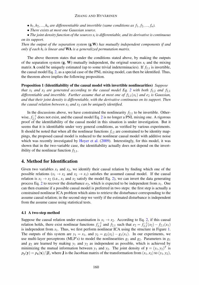
is independent from x1. Thus, we first perform nonlinear ICA using the structure in Figure 1.The outputs of this system are y1 = x1, and y2 = g2(x2)− g1(x1). In our experiments, weuse multi-layer perceptrons (MLP’s) to model the nonlinearities g1 and g2. Parameters in g1and g2 are learned by making y1 and y2 as independent as possible, which is achieved byminimizing the mutual information between y1 and y2. The joint density of y = (y1,y2)

T ispy(y) = px(x)/|J|, where J is the Jacobian matrix of the transformation from (x1,x2) to (y1,y2),

160

NONLINEAR ACYCLIC CAUSAL MODELS

i.e., J =[∂ (y1,y2)

/∂ (x1,x2)

]. Clearly |J|= |g′2|. The joint entropy of y is then

H(y) =−E{log py(y)}=−E{log px(x)− log |J|}= H(x)+E{log |J|}.

Finally, the mutual information between y1 and y2 is

I(y1,y2) = H(y1)+H(y2)−H(y)= H(y1)+H(y2)−E{log |J|}−H(x)= −E{py1(y1)}−E{py2(y2)}−E{log |g′2|}−H(x),

where H(x) does not depend on the parameters in g1 and g2 and can be considered as constant.One can easily find the gradient of I(y1,y2) w.r.t. the parameters in g1 and g2, and minimizeI(y1,y2) using gradient-descent methods. Details of the algorithm are skipped.

x2

x1

g1

+-

g2

y1

y2

Figure 1: The constrained nonlinearICA system used to verifyif the causal relation x1→x2 holds.

y1 and y2 produced by the first step are the assumedcause and the estimated corresponding disturbance, re-spectively. In the second step, one needs to verify if theyare independent, using statistical independence tests. Weadopt the kernel-based statistical test (Gretton et al.,2008), with the significance level α = 0.01. If y1 andy2 are not independent, indicating that x1→ x2 does nothold, we repeat the above procedure (with x1 and x2 ex-changed) to verify if x2 → x1 holds. If y1 and y2 areindependent, usually we can conclude that x1 causes x2,and that g1 and g2 provide an estimate of f2,1 and f−1

2,2 ,respectively. However, it is possible that both x1→ x2 and x2→ x1 hold, although the chance isvery small. Therefore, for the sake of reliability, in this situation we also test if x2→ x1 holds.Finally, we can find the relationship between x1 and x2 among all four possible scenarios: 1.x1 → x2, 2. x2 → x1, 3. both causal relations are possible, and 4. there is no causal relationbetween x1 and x2 which follows our model.

4.2 Practical considerations

The first issue that needs considering in practical implementation of our method is the modelcomplexity, which is controlled by the number of hidden units in the MLP’s modelling g1 andg2 in Figure 1. The system should have enough flexibility, and at the same time, to avoidoverfitting, it should be as simple as possible. To this end, two ways are used. One is 10-foldcross-validation. The other is heuristic: we try different numbers of hidden units in a reasonablerange (say, between 4 and 10); if the resulting causal relation does not change, we conclude thatthe result is feasible.

The second issue is the initialization of the nonlinearities g1 and g2 in Figure 1. If the non-linear distortions f2,2 and f2,1 are very strong, it may take a long time for the nonlinear ICAalgorithm in the first step to converge, and it is also possible that the algorithm converges toa local optimum. This can be avoided by using reasonable initializations for g1 and g2. Twoschemes are used in our experiments. One is motivated by visual inspection of the data distri-bution: we simply use a logarithm-like function to initialize g1 and g2 to make the transformeddata more regular. The other is by making use of Gaussianization (Zhang and Chan, 2005).Roughly speaking, the central limit theorem states that sums of independent variables tend tobe Gaussian. Since f−1

2,2 (x2) in the causal model Eq. 2 is the sum of two independent variables,it is expected to be not very far from Gaussian. Therefore, for each variable which is very farfrom Gaussian, its associated nonlinearity (g1 or g2 in Figure 1) is initialized by the strictly

161

ZHANG AND HYVÄRINEN

Data Set #1 #2 #3 #4 #5 #6 #7 #8Result x1→ x2 x1→ x2 x1→ x2 x1←‡ x2 x1← x2 x1→ x2 x1← x2 x1→ x2

Table 1: Causal directions obtained. (‡ indicates that the causal relation is not significant.)

increasing function transforming this variable to standard Gaussian. In all experiments, thesetwo schemes give the same final results.

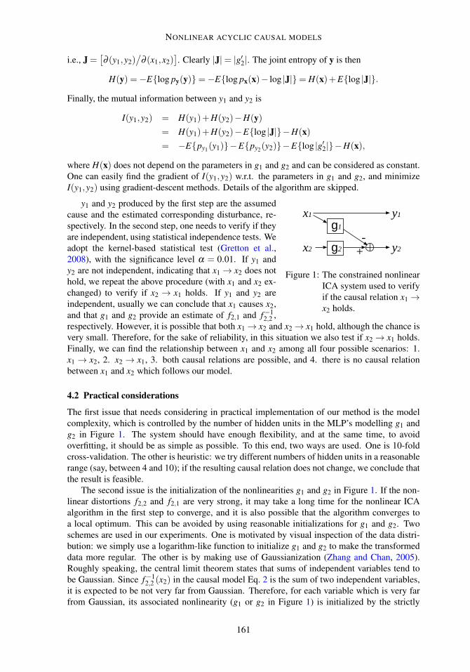
5. ResultsThe proposed nonlinear causal discovery method has been applied to the “CauseEffectPairs"task proposed by Mooij et al. (2008) in the Pot-luck challenge. In this task, eight data sets aregiven; each of them contains the observed values of two variables x1 and x2. The goal is todistinguish the cause from the effect for each data set. Figure 2 gives the scatterplots of x1 andx2 in all the eight data sets. Table 1 summaries our results. In particular, below we take datasets 1 and 8 as examples to illustrate the performance of our method.

0 1000 2000

0

5

10

Data Set 1

x 2 0 1000 2000500

1000

1500

2000Data Set 2

8 10 12 14

0

5

10

Data Set 3

1100 1400 170017000

1000

2000

Data Set 4

0.2 0.4 0.6 0.8

510152025

Data Set 5

5 10 15 20 25

0.20.40.60.8

1Data Set 6

x1

0.2 0.4 0.6

510152025

Data Set 7

20 40 60 80

2000400060008000

Data Set 8

Figure 2: Scatterplot of x1 and x2 in each data set of the “CauseEffectPairs" task (Mooij et al.,2008).

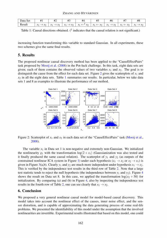
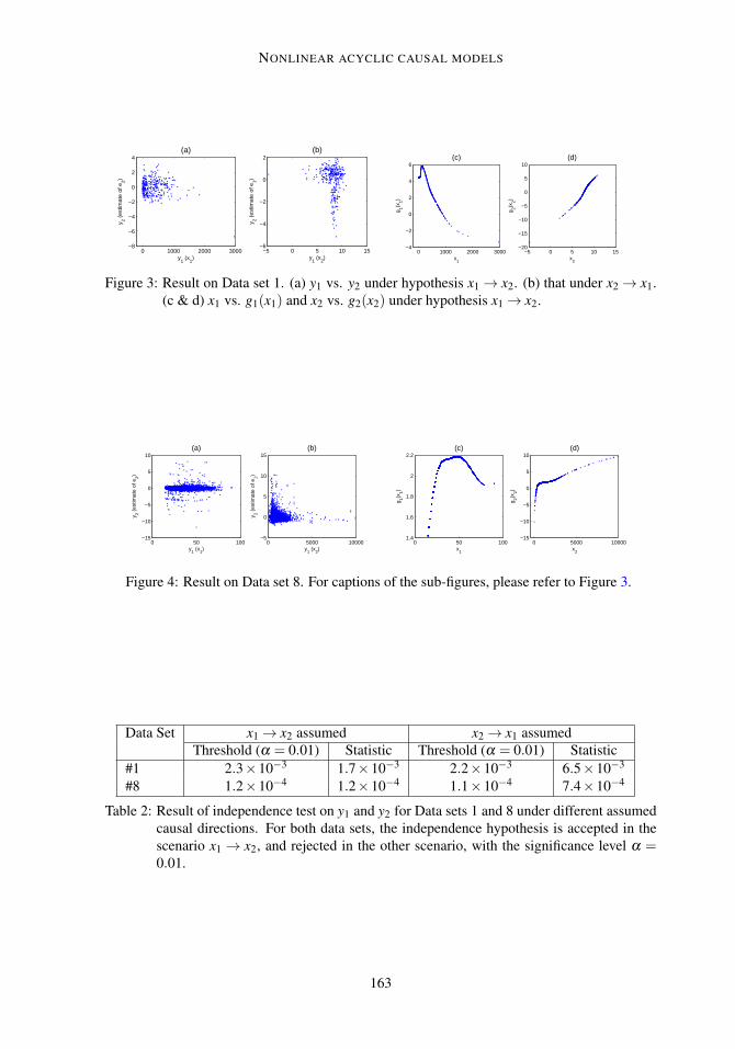
The variable x1 in Data set 1 is non-negative and extremely non-Gaussian. We initializedthe nonlinearity g1 with the transformation log(2+ x1) (Gaussianization was also tested andit finally produced the same causal relation). The scatterplot of y1 and y2 (as outputs of theconstrained nonlinear ICA system in Figure 1) under each hypothesis (x1 → x2 or x2 → x1) isgiven in Figure 3(a,b). Clearly y1 and y2 are much more independent under hypothesis x1→ x2.This is verified by the independence test results in the third row of Table 2. Note that a largetest statistic tends to reject the null hypothesis (the independence between y1 and y2). Figure 4shows the result on Data set 8. In this case, we applied the transformation log(x2 + 50) forinitialization. By comparing (a) and (b) in Figure 4, also by inspecting the independence testresults in the fourth row of Table 2, one can see clearly that x1→ x2.

6. ConclusionWe proposed a very general nonlinear causal model for model-based causal discovery. Thismodel takes into account the nonlinear effect of the causes, inner noise effect, and the sen-sor distortion, and is capable of approximating the data generating process of some real-lifeproblems. We presented the identifiability of this model under the assumption that the involvednonlinearities are invertible. Experimental results illustrated that based on this model, one could

162

NONLINEAR ACYCLIC CAUSAL MODELS

0 1000 2000 3000−8

−6

−4

−2

0

2

4

y 2 (es

timat

e of

e2)

(a)

y1 (x

1)

−5 0 5 10 15−6

−4

−2

0

2

y1 (x

2)

y 2 (es

timat

e of

e1)

(b)

0 1000 2000 3000−4

−2

0

2

4

6

x1

g 1(x1)

(c)

−5 0 5 10 15−20

−15

−10

−5

0

5

10

x2

g 2(x2)

(d)

Figure 3: Result on Data set 1. (a) y1 vs. y2 under hypothesis x1→ x2. (b) that under x2→ x1.(c & d) x1 vs. g1(x1) and x2 vs. g2(x2) under hypothesis x1→ x2.

0 50 100−15

−10

−5

0

5

10

y 2 (es

timat

e of

e2)

y1 (x

1)

(a)

0 5000 10000−5

0

5

10

15

y1 (x

2)

y 2 (es

timat

e of

e1)

(b)

0 50 1001.4

1.6

1.8

2

2.2

x1

g 1(x1)

(c)

0 5000 10000−15

−10

−5

0

5

10

x2

g 2(x2)

(d)

Figure 4: Result on Data set 8. For captions of the sub-figures, please refer to Figure 3.

Data Set x1→ x2 assumed x2→ x1 assumedThreshold (α = 0.01) Statistic Threshold (α = 0.01) Statistic

#1 2.3×10−3 1.7×10−3 2.2×10−3 6.5×10−3

#8 1.2×10−4 1.2×10−4 1.1×10−4 7.4×10−4

Table 2: Result of independence test on y1 and y2 for Data sets 1 and 8 under different assumedcausal directions. For both data sets, the independence hypothesis is accepted in thescenario x1 → x2, and rejected in the other scenario, with the significance level α =0.01.

163

ZHANG AND HYVÄRINEN

successfully distinguish the cause from the effect, even if the nonlinear function of the cause isnot invertible. An on-going work is to investigate the identifiability of this model under moregeneral conditions.

ReferencesS. Achard and C. Jutten. Identifiability of post-nonlinear mixtures. IEEE Signal Processing

Letters, 12:423–426, 2005.

C. Granger. Testing for causality: A personal viewpoint. Journal of Economic Dynamics andControl, 2, 1980.

A. Gretton, K. Fukumizu, C.H. Teo, L. Song, B. Schölkopf, and A.J. Smola. A kernel statisticaltest of independence. In NIPS 20, pages 585–592, Cambridge, MA, 2008.

P.O. Hoyer, D. Janzing, J. Mooji, J. Peters, and B. Schölkopf. Nonlinear causal discovery withadditive noise models. In NIPS 21, Vancouver, B.C., Canada, 2009. To appear.

A. Hyvärinen and P. Pajunen. Nonlinear independent component analysis: Existence anduniqueness results. Neural Networks, 12(3):429–439, 1999.

A. Hyvärinen, J. Karhunen, and E. Oja. Independent Component Analysis. John Wiley & Sons,Inc, 2001.

C. Jutten and A. Taleb. Source separation: From dusk till dawn. In 2nd International Workshopon Independent Component Analysis and Blind Signal Separation (ICA 2000), pages 15–26,Helsinki, Finland, 2000.

J. Mooij, D. Janzing, and B. Schölkopf. Distinguishing between cause and effect,Oct. 2008. URL http://www.kyb.tuebingen.mpg.de/bs/people/jorism/causality-data/.

J. Pearl. Causality: Models, Reasoning, and Inference. Cambridge University Press, Cam-bridge, 2000.

S. Shimizu, P.O. Hoyer, A. Hyvärinen, and A.J. Kerminen. A linear non-Gaussian acyclic modelfor causal discovery. Journal of Machine Learning Research, 7:2003–2030, 2006.

P. Spirtes, C. Glymour, and R. Scheines. Causation, Prediction, and Search. MIT Press, Cam-bridge, MA, 2nd edition edition, 2000.

A. Taleb and C. Jutten. Source separation in post-nonlinear mixtures. IEEE Trans. on SignalProcessing, 47(10):2807–2820, 1999.

K. Zhang and L. W. Chan. Extended Gaussianization method for blind separation of post-nonlinear mixtures. Neural Computation, 17(2):425–452, 2005.

K. Zhang and A. Hyvärinen. On the identifiability of the post-nonlinear causal model. InProc. 25th Conference on Uncertainty in Artificial Intelligence (UAI), Montreal, Canada,June 2009.

164