chalmers - core.ac.uk · institutionen för elkraftteknik chalmers tekniska hÖgskola 412 96...
TRANSCRIPT

CHALMERS
Mitigation of Power-Frequency Magnetic Fields
With Applications to Substations and Other Parts of the Electric Network
ENER SALINAS
Department of Electric Power Engineering Chalmers University of Technology Göteborg, Sweden 2001

Mitigation of Power-Frequency Magnetic Fields
With Applications to Substations and Other Parts of the Electric Network
av
Ener Salinas
Akademisk avhandling som för avläggande av teknisk doktorsexamen vid Chalmers tekniska högskola
försvaras vid en offentlig disputation i IT-rummet, Hörsalsvägen 11 Chalmers tekniska högskolan, Göteborg,
fredagen den 24: e augusti 2001, kl 10.00.
Fakultetsopponent är Michel Ianoz, Laboratoire de Réseaux d'Energie Electrique
Ecole Polytechnique Federale de Lausanne, Schweiz.
Avhandlingen finns tillgänglig på Institutionen för Elkraftteknik
CHALMERS TEKNISKA HÖGSKOLA 412 96 Göteborg
Telefon 031-7721660

Abstract
––––––––––––––––––––––––––––––––––––––––
n recent times, electromagnetic emissions from various electrical
I components have induced more than one debate whether they represent a harmful influence to our health. In addition, interferences caused by power frequency magnetic fields (PFMFs) on electron beam based electronic equipment (e.g. cathode ray tubes found in TV screens and computer monitors, electron microscopes) become evident at levels over 1 microtesla. These issues have caused some concern with the general public but also to the utilities, their customers and the electromagnetic compatibility community. On the other hand, they have also spurred efforts to study and mitigate these fields. Although most published studies and debates are concerned with fields from power transmission lines, similar levels of PFMFs can be found in a city neighbourhood. For this reason this study focuses on the fields originating from the last stages of the power network before reaching the customer, in particular the components of in-house secondary substa-tions. However the methods developed in this study can also be applied more generally. Conductive and ferromagnetic shielding, passive and active compensa-tion and other techniques are described. These techniques make use of modern methods of analysis such as algebraic computing and 2D/3D modelling. It was found that shielding using thin conductive plates and a proper design can provide for cost-effective mitigation of PFMFs. It was shown that the choice of either ferromagnetic or conductive shielding is dependant on a number of variables, which can only be determined by a proper 2D or 3D modelling. It was also found that cable and busbar connections and not the transformers are the main cause of large PFMF emission from substations. These and other results were applied to actual cases where the measured values were considered as problematic, or where low emission was a requirement already at the design stages. Keywords: busbars, eddy currents, EMC, FEM, field mitigation, power-frequency magnetic fields, substation, transformers.
Preface n this thesis a research project is described which was both pleasant and rewarding. The project started as an initiative to deal with a difficult and an interesting issue: How to mitigate power-frequency magnetic fields? Search for solutions could work best if efforts were combined. This resulted in a co-operation between industry and the academic world. The departments of Electric Power Engineering and Electromagnetics at Chalmers University of Technology, Elforsk, ABB and Göteborg Energi, together initiated this project.
I
I would like to thank Elforsk for financing this project. My gratitude goes to the members of the steering group: Lars Hammarsson (Göteborg Energi Nät AB), Sven Hörnfeldt (ABB Corporate Research AB) and Jan-Olov Sjödin (Vattenfall Transmission AB), for the continuous assessment of the project, their good advice and helpful meetings.
In order to find the optimal solution of a problem sometimes more than one point of view is needed. In this respect it has been quite an experience to have the advise of my three supervisors, Professors Jaap Daalder, Anders Bondeson and Yngve Hamnerius, each of them with a rather different, yet necessary, background for a of project of this nature. I would like to express my gratitude to each of you.
I would like to thank Lars Aspemyr and professor Jorma Luomi for their cooperation during the initial stages of the project, professor Eskil Möller for our discussions about modelling with Opera 3D, Aleksander Bartnicki, for the help and checks in some of our experiments, and the personal at Göteborg Energi for their technical support.
I am grateful to Kjell Siimon, Jan-Olov Lantto and Alexander Wolgast, for countless times of assistance in computer magic.
Finally, dear colleagues and friends at this institute, whom through discussions at the coffee room (some of them about electricity), brännboll games, and lunches at Primavera, created such a nice working atmosphere, to all of you: Thanks!

Table of contents
1. Introduction 1 2. Sources of power frequency magnetic fields 9
3. Interactions 19
4. Visualization of mitigation methods 29
5. PFMFs originating from secondary substations 37
6. Phase arrangements 43
7. Modelling PFMFs using 2D and 3D FEM codes 49
8. PFMFs from busbars 61
9. Conductive and ferromagnetic shielding 67
10. Active and passive compensation 89
11. Mitigating the field of transformers 97
12. Examples of field mitigation 109
13. Extensions of this work 135
14. Conclusions 137
Apendixes 139 Included papers 149

1 Introduction ––––––––––––––––––––––––––––––––––––––––
ome time ago, during a conversation with an experimental physicist
we arrived at the conclusion that there are two things one certainly
always remembers. One of them is the first time you saw a magnet – I
still vividly recall playing with iron fillings on a paper while moving a
magnetized screw under it. The other one is of a non-technical nature and
is not the subject of this thesis.
S
This report is about magnetism, a subject that has fascinated humans for
centuries, and still does. Recently I managed to establish a little record of
7.5 minutes in levitating a spinning magnet that was constructed in
collaboration with my first year students [1]. No batteries,
superconductors or cold temperatures were involved, just a trick of pure
magnetism: one magnet on top of another facing the same poles. Rotation
and precession, contribute to the stability of this “toy”. Devices such as
this were thought to be physically impossible until just a couple of
decades ago.
Fig. 1.1 A magnetic spinning top is stably levitating above a larger ring magnet. No batteries, cold temperatures or superconductors are added. Just pure magnetism!
1

Magnetism itself has of course been known since ancient times. The
Chinese called the magnetic stones tzhu shih, or “love”. In French a
magnet goes by the name aimant, the word for “loving” or “affectionate”.
In my hometown, Arequipa, the word is imán, which also means “very
popular” or “attractive”. Then again, we won’t go deeper into this
subject.
As advanced as our science and technology is, one may think that nearly
everything is known about magnetism. However, there are still
interesting, yet unresolved problems. Take for example something we
have all heard of: the earth’s magnetism. First of all, in most of our
school textbooks, earth’s magnetism is portrayed as our planet being a
big magnet. This may be a misconception. To our best knowledge the
representation of earth’s magnetism is closest to an electromagnet:
circulating ionic currents (billions of amperes) furnish the magnetic field.
Yet, we are not very sure about the details of this model. Another
example: if we were ever sure that the magnetism of rocks called
magnetite or lodestone were originated by the earth’s magnetic field, then
we have to be prepared to encounter another problem; namely that the
earth’s magnetic field is simply too weak to produce the magnetization
found in some of these stones. A scenario involving lightning may solve
this puzzle: hundreds of millions volts and hundreds of thousands
amperes certainly are able to induce high magnetization in rocks rich in
iron. To work out the details of this hypothesis is the exciting part.
2

1.1 The electromagnetic revolution The moment that represented the start of one of the most important
revolutions in science and in due time having profound implications on
technology, was not an Eureka! in the Archimedes style, nor a logically
deducted theoretical result more in the spirit of Newton or Einstein. No,
it was simply an “accident”, during a routine preparation for a physics
demonstration. The Danish physicist Hans Christian Oersted, observed in
1820 that when an electric current was switched on, a nearby magnetic
compass needle started to move. Although he was not able to explain this
phenomenon, he published his perception never realizing that 18 years
before (!), Gian Dominico Romognosi had already made the very same
observation. Moreover Romognosi published it in La Gazetta de
Trentino. Unfortunately, two things contributed for this observation to be
overlooked: Romognosi was a jurist, and he published in a newspaper.
Only a few days passed since the receipt of the news of Oersted’s
discovery in Paris, when André Marie Ampère presented to the French
academy a list of new results based on Oersted’s observations; including
the one involving attraction between conductors. In England Michael
Faraday constructed the first device that could move continuously with
electricity [2], and, not much later, he proved the existence of
electromagnetic induction, inventing at the same time the transformer. A
flurry of investigation ignited and soon other results were obtained,
culminating brilliantly with the synthesis and unification of all
electromagnetic phenomena by James C. Maxwell in 1871. Strangely
enough, no conservative opposition arose to this revolution; neither was
3

there a time of gradual acceptance as for example happened with the
Copernican revolution [3]. In fact it seemed the world was prepared and
waiting for it.
1.2 Power-frequency magnetic fields – an uninvited guest? The electromagnetic revolution changed technology to the world of
electricity, electronics and communication we know today. This technical
world brought also circuit boards, cables, data transferring devices,
power transmission lines, antennas and highly packed circuits – to
mention a few. Oersted’s and Faraday’s observations imply that these
devices, due to their electromagnetic properties, are fated to interfere
with each other. Moreover, there are propagating electric and magnetic
fields that escape the working frequency band of a device or a circuit (i.e.
fields due to harmonics).
These fields, depending on their frequency, have different types of
interactions with matter and are in general, for more than one reason,
undesirable. It is natural to ask if these fields can be hostile to living
organisms and if they can produce interference to electronic equipment.
As will be seen in chapter 3 the answers to these questions are not trivial.
Total elimination of these fields could mean to influence the cause of
them so drastically that the devices producing them would not be of
much use (e.g. some field may leak off a motor inducing disturbances on
some electronic devices, but altering the currents that originate this stray
field could also make the motor stop). However it is clear that reducing
these fields in a suitable way would be very much desired.
4

1.3 Mitigation of power-frequency magnetic fields Imagine you are very annoyed by the noise caused by your neighbour
who is fond of music and dance. One way to solve the problems is by
covering the walls with sound-masking material (such as fibre-glass
sound attenuator laminates or cellulose treated with borax or aluminium
sulphate). You can also talk to your neighbour about possible solutions,
modifying his music schedule, turning down the volume of the devices or
simply moving that big stereo to the other side of the room.
Noise attenuation is just an analogy to illustrate the methodology used in
this project. The standard method in magnetic field reduction is to shield
affected areas, often using aluminium or iron laminations. The project
described in this report goes beyond this criterion. Properties of magnetic
field sources are studied; reasons leading to the generation of high fields
are investigated; subsequently a cost-efficient strategy to reduce these
fields is developed. Simple tools sometimes sufficiently attain large field
reductions. However, extensive experimentation and laborious numerical
simulations are, not infrequently, necessary to reach modest – but
valuable – mitigation factors.
Although this report focuses on the magnetic field reduction from
secondary substations, the methods explained here can be applied to
other parts of the electric network. An electrical secondary substation is
described as the last segment of the distribution stages and closest to the
customer.
5

1.4 Outline of this report
Chapter 2 studies typical sources of power frequency magnetic fields.
Deduced properties from this study are essential for developing field
reduction strategies. Chapter 3 is dedicated to the interaction between
electromagnetic fields and matter, biological effects and electromagnetic
compatibility (EMC). Chapter 4 presents simple experiments to
intuitively visualize some of the techniques used in this project such as
shielding (conductive and ferromagnetic) and active compensation.
Chapter 5 describes the fields produced by a substation. The relevance of
field reduction by phase arrangement, phase splitting, and optimal
positioning of the sources is analysed in chapter 6.
Numerical methods and fundamentals of finite element codes are
described in chapter 7. A set of properties for the field of busbars is
obtained in chapter 8. In chapter 9, 2D and 3D FEM codes are applied to
the conductive and ferromagnetic shielding of magnetic fields from
various sources, especially of busbars. Analysis of induced currents in
conductive shielding suggests the structure of some of the circuits to be
used in passive and active compensation, the subject of chapter 10.
Chapter 11 deals with the field mitigation of transformers. Chapter 12
presents applications to actual cases of field reduction, among others,
from newly built, modified and renovated substations. Screens for
shielding can also be built using a multiple-layer structure. These and
other additional characteristics are presented in the appendixes. Chapter
13 discusses future extensions of this work. Chapter 14 presents the main
conclusions. At the end published articles are attached.
6

Throughout this report, the main physical quantity involved is the
magnetic flux density (B). In most cases, for simplicity, it is called
merely magnetic field. MKS units are used thorough out. Moreover, for
B, microtesla (µT) is the most useful sub-unit. Another quantity used is
the magnetic field strength (H), with units: A/m. If there is no material
around, then there is no actual reason to prefer H or B since they are
related by B = µ0H. However, inside materials, the distinction can be
important.
Some abbreviations used in this report are:
PFMFs: Power frequency magnetic fields
EMC: Electromagnetic compatibility
Mitigation, reduction and attenuation are used as synonyms, as are
shielding and screening but the latter entail the application of metallic
plates.
References [1] E. Salinas, et al, “Mechanical and Magnetic Levitation”, in: First Quest, First year students project at the ED-Section, Chalmers University of Technology, Sweden, 2000. [2] J. F. Keithley The Story of Electrical and Magnetic Measurements IEEE Press, New York, 1999. [3] T. S. Kuhn, The Structure of Scientific Revolutions, The University of Chicago Press, 1962.
7

8

2 Sources of power frequency magnetic fields
––––––––––––––––––––––––––––––––––––––––
he sources of PFMFs associated with electric energy flows are:
T
transmission lines, overhead distribution services, underground cables,busbars (often carrying currents of the order of few to several thousands
amperes), transformers, and in-house cables (Fig. 2.1). In order to design
strategies of field reduction it is important to study the properties,
similarities and differences of these sources. Although sometimes
difficult it is possible – at least in principle – to estimate the magnetic
field emitted by most of these sources rather accurately, the most difficult
one being the field of a transformer. Different degrees of approximation
are required depending on each particular case. For long systems, as in
the case of transmission lines or underground cables, a two-dimensional
(2D) treatment suffices. However for short busbars, where edge effects
are important, or in the case of transformers, three-dimensional (3D)
treatments are necessary. These estimations can, in a few cases, be
obtained analytically, or using symbolic manipulation programs.
However, numerical codes are usually very effective for complex cases.
To evaluate the field from the devices mentioned above it is helpful to
find the magnetic field produced by a small element (i.e. of infinitesimal
length) of current. This can be done using the Ampere-Laplace law [1],
often also called the Biot-Savart formula [2]:
9

2
4 rdid r0 elB ×
=
πµ
(2.1)
Conductors
Overhead distribution
Transmission line
Underground cables
Connections
Transformers
Busbars
Fig. 2. 1 Major sources of PFMFs at the transmission and distribution stages.
The direction of the current i is represented by dl, and r = r er is the
position where the field B is evaluated (Fig. 2.2). Once the field from this
element of current is determined, it is a matter of using the superposition
10

principle and integration to obtain the magnetic field from a more
complex source. However, an inspection of this picture and Eq. 2.1 gives
what appears to be a physical impossibility, or a contradiction, as the
segment represents a broken circuit the current appears on one edge and
disappears on the other edge (Fig. 2.2). Consequently the system seems
to violate the continuity equation and charge conservation.
B
r
i
dl
Fig. 2. 2 The field of a small element of current.
Two different ways to solve this apparent contradiction are presented in
appendix I.
2.1 Magnetic field of a straight wire of length L A finite, very thin, and straight conductor of length L carries a current i.
It is placed along the z-axis (Fig. 2.3). The magnetic field [3] at the
location (ρ, z) is independent of the coordinate φ. Its magnitude and
direction, in cylindrical coordinates, is given by:
φρρρπ
µρ eB
+−−
+++
+=
2222
0
)2/(2/
)2/(2/
4),(
zLzL
zLzLiz (2.2)
11

B
ρ
z
x
y
i
L φ
Fig. 2.3 Magnetic field of a thin, straight wire of length L.
2.2 Magnetic field of an infinite wire
In order to obtain the field of an infinite (or very long) wire, it is helpful
to evaluate Eq. 2.2 in the plane perpendicular to the centre of the wire
(i.e. at z = 0). The result is a simplified expression
φρρπ
µρ eB
+=
22
0
)2/(4)0,(
LLi
(2.3)
Hence when L → ∞, or when ρ<< L, the last equation expresses the field
of an infinite long wire. For this limit, the equation becomes even simpler
φρπµρ eB2
)( 0i= (2.4)
The decay of the magnetic field from this source is explicitly – unlike the
field for short wires – inversely proportional to the distance.
12

2.2 Magnetic field of two finite wires carrying a mono-phase
current The aim is to evaluate the magnetic field, and its dependence on the
distance, of two parallel wires carrying a single phase current, one wire
carries a current i and the other carries the return -i. First of all, the field
of two finite wires (with length L) is evaluated. In practical situations, it
can be advantageous to use Cartesian coordinates (x, y, z). In such case
Eq. 2.2 has the following expression
),,()(4
),,( 0 zyxfxyizyx yx eeB +−=π
µ (2.5)
where
−++−
++++
++
=22222222 )2/(
2/)2/(
2/)(
1),,(
zLyxzL
zLyxzL
yxzyxf
For a two wires configuration with a separation a (Fig. 2.4) both field
contributions will superimpose
[ ] [{ }yx zyxfxzyxfxzyxfyzyxfyi eeB ),,(),,((),,(),,((4 2222111122221111
0
−++−=π
]µ
The following relations hold: 2/1 axx −= ; 2/2 axx += ; ;
.
yyy == 21
zzz == 21
In order to study the field decay with distance, e.g. along the y-axis, the
calculation is specialized for 0=z and 0=x (i.e. 2/1 ax −= , ). 2/2 ax =
13

B
a
+i
z
x
y
L
2 1
-i
Fig. 2.4 Magnetic field of two parallel wires of length L, the directions of the instantaneous currents are also shown.
Then the field component along the x-axis vanishes, leaving a simple
expression for the field of two parallel wires of finite length
( )[ ] ( ) yLyaya
aLiy eB
+++−=
22222
0
)2/(2/2/4)0,,0(
πµ (2.6)
Furthermore, for long wires y << L the formula reduces to:
( )[ yyaaiy eB
+−=
22
0
2/2)0,,0(
πµ (2.7) ]
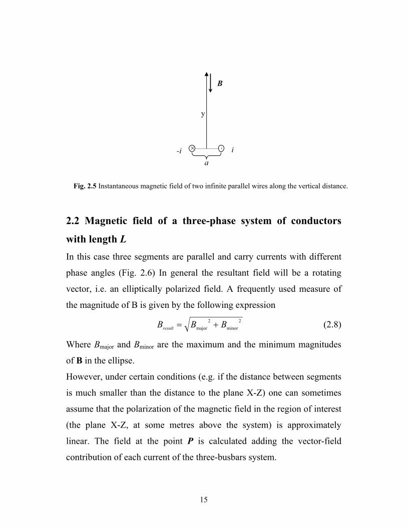
For vertical distances y much larger than the separation a (Fig. 2.5),
which is often the case of interest, two facts can be deduced: firstly, the
magnetic field depends linearly on the separation a; and secondly, the
magnetic field decays as 1/(distance)2, this is a much faster decay than
the dependence on the distance of the field of a single line.
14
B
× ·
y
a i -i
Fig. 2.5 Instantaneous magnetic field of two infinite parallel wires along the vertical distance.
2.2 Magnetic field of a three-phase system of conductors
with length L In this case three segments are parallel and carry currents with different
phase angles (Fig. 2.6) In general the resultant field will be a rotating
vector, i.e. an elliptically polarized field. A frequently used measure of
the magnitude of B is given by the following expression 2
minor2
major BBBresult += (2.8)
Where Bmajor and Bminor are the maximum and the minimum magnitudes
of B in the ellipse.
However, under certain conditions (e.g. if the distance between segments
is much smaller than the distance to the plane X-Z) one can sometimes
assume that the polarization of the magnetic field in the region of interest
(the plane X-Z, at some metres above the system) is approximately
linear. The field at the point P is calculated adding the vector-field
contribution of each current of the three-busbars system.
15

T
S R
P
Lz
y
x
Z
X
Y
Fig. 2. 6 Magnetic field of a three-phase system of wires evaluated at the point P. The resulting field is rotating and elliptically polarized.
After some lengthy but straightforward calculations, using Eq. 2.5, the
rms-value of the magnetic field, in microtesla, acquires the following
expression:
r B Total(x,y)
rms=
irms
10• A1 −A2
2−A3
2
2
+ C1 −C2
2−C3
2
2
+34
A2−A3( )2+ C2−C3( )2[ ]
1/2
where,
3,2,1,)2/(
2/
)2/(
2/),
)2/(
2/
)2/(
2/),
22222222
22222222
=
−++
−+
+++
++
−=
−++
−+
+++
++
=
kzLyx
zL
zLyx
zLyx
yyx
zLyx
zL
zLyx
zLyx
xyx
kkk
k
kkk
(
(
C
A
k
k (2.9)
16

This equation is easy to program for a computer, for example MAPLE VI
(which is a symbolic manipulation language), thus making it possible to
evaluate the field from any geometrical arrangement of straight
conductors within the mentioned approximation. By analysing the
dependence on some parameters (e.g. the distance between busbars, the
length of the busbars, the distance from the busbars system to the
measuring point) it is possible to gain some understanding of the
properties of busbars.
For a more realistic study of busbars (e.g. considering their finite
thickness); for the computation of the field originating from coils of
transformers, and other complex problems involving conductors, 2D and
3D numerical simulations are used (to be described in subsequent
chapters). However even the formulations of numerical codes that can be
able to perform such computations are based on the results discussed in
this chapter.
References
[1] J. D. Jackson, Classical Electrodynamics, Third Edition, John Wiley
& Sons, Inc. N.Y. 1999, pp. 175-180.
[2] D. K. Cheng, Field and Wave Electromagnetics, Addison-Wesley
Massachusetts, 1989, pp. 600-605.
[3] E. Salinas, Reduction of Power Frequency Magnetic Fields from
Electrical Secondary Substations, Tek. Lic. Thesis, Chalmers University
of Technology, ED section, 1999, pp. 25-32.
17

18

3 Interactions ––––––––––––––––––––––––––––––––––––––––
ources of electromagnetic fields can produce radiant fields and S
non-radiant fields. A radiant field persists even after the source is turned
off; this behaviour is typical for distances (D) much larger than the
wavelength λ (i.e. D/λ >> 1 or “far-field” region). A non-radiant field,
typical for sources with D/λ << 1 (also called “near-field” region),
produces electric and magnetic fields that can be decoupled and treated
as independent entities. The wavelength of a field with a frequency of 50
Hz is λ = c / f = 6000 Km. This distance is as large as the radius of our
planet (Fig. 3.1). The cases of interest in this study are phenomena taking
place at a “human-size” scale; thus the frequency is certainly within the
near field region. Moreover, the interest is on the magnetic field part of
the PFMF. The electric field is also part of it, but is of little interest in
50 Hz
λ
Fig. 3.1 The wavelength of an electromagnetic field with a frequency of 50 Hz is nearly as large as the radius of the earth.
19

this study. Electric fields caused by free charges can easily be shielded by
conducting objects and have poor ability to penetrate walls and even
skin.
3.1 The electromagnetic spectrum
In particular for PFMFs, there are two relevant interactions: i) the
influence of PFMFs on living beings and ii) on electronic equipment. In
order to determine (or at least try to comprehend) these interactions it is
essential to characterize PFMFs in the context of a broad collection of
fields, namely the electromagnetic spectrum.
The electromagnetic spectrum represents all possible energies a photon
can have (Fig. 3.2). The interest of this study (50/60 Hz) belongs to a
narrow range of this spectrum called extremely low frequency (ELF).
From the energy point of view these frequencies belong to nearly the
lowest end of the spectrum – even far lower than the range of radio
waves.
The upper part of the spectrum contains ionizing radiation. The
frequency (and consequently the energy per quantum) of this type of
radiation is substantially higher than that of visible light, and is therefore
able to penetrate many materials. When these rays interact with atoms,
they send off electrons producing ions, thus the name “ionizing”. High
energetic ultraviolet radiation usually manages to kick off external
electrons; X-rays penetrate more and can hit electrons belonging to
interior energy levels. In extreme cases (e.g. gamma radiation) they can
affect the nucleus and induce a nuclear reaction. Because ionization of
20
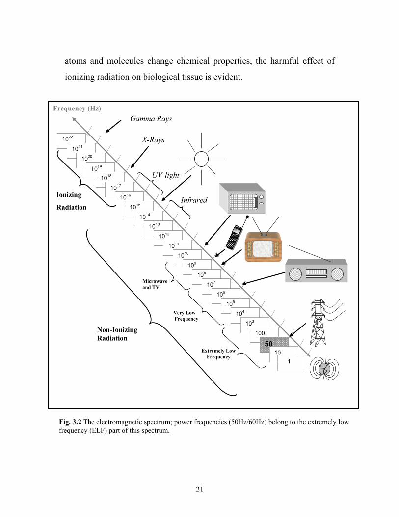
atoms and molecules change chemical properties, the harmful effect of
ionizing radiation on biological tissue is evident.
Non-Ionizing Radiation
Ionizing
Radiation
Extremely Low Frequency
Very Low Frequency
Microwave and TV
UV-light
1
X-Rays
Gamma Rays
50 10
100 103
104 105
106 107
108 109
1010 1011
1012 1013
1014 1015
1016 1017
1018 1019
1020 1021
1022
Infrared
Frequency (Hz)
Fig. 3.2 The electromagnetic spectrum; power frequencies (50Hz/60Hz) belong to the extremely low frequency (ELF) part of this spectrum.
21

Different astrophysical phenomena are the major sources of ionizing
radiation. It originates, and remains (thanks to the shielding properties of
our atmosphere at these frequencies), mainly in space. However gamma
and X-ray emissions occur to some extent in radioactive matter on earth;
X-rays are also emitted by certain electronic devices.
Non-ionizing radiation represents electromagnetic waves at lower
frequencies, where each quantum is not energetic enough to get electrons
away from the atoms. Yet, at some frequencies, some physical
mechanism, different from the ones described for the ionizing radiation,
can operate. An example is the rapid increase of temperature (induced by
rotation of water molecules) in biological tissue when exposed to certain
ranges of microwave radiation. A large source of non-ionizing radiation
comes from space and especially our sun. Other sources that emit non-
ionizing radiation are electronic devices, TV-sets, mobile telephones,
radio transmitters, power lines, to name a few.
Static (zero frequency) magnetic fields, such as the geomagnetic, do not
induce forces on non-moving charges. However, the real world is
dynamic, thus some interaction is expected. Fortunately, this field has
been part of the external environment that shaped life on our planet.
Thus, even though the average geomagnetic field (around 20-50
microtesla) is fifty times larger than the range of PFMFs considered
problematic, living organisms are accustomed to it!
3.2 Biological effects of PFMFs Studies [1] have shown that power frequency magnetic fields may
produce biological effects. Furthermore, it is suspected that different
22

kinds of diseases might be related to PFMFs, such as: brain cancer and
leukaemia. The values of the magnetic field involved are also dependent
on the type of analysis. In some epidemiological studies, values as low as
0.2 microtesla, are mentioned to correlate with significant increase in
cancer incidence among populations living nearby power lines [2]. Today
several experiments are being conducted on animals and researchers have
indicated that under certain circumstances exposure to PFMFs may
promote tumour development. However other investigators have failed in
reproducing these results.
IARC (International Agency for Research on Cancer) recently [3]
evaluated possible carcinogenic hazards to human beings from exposures
to static and extremely low frequency ELFelectric and magnetic fields,
issuing that:
“Overall, ELF magnetic fields were evaluated as possibly carcinogenic
to humans, based on the statistical association of higher level residential
ELF magnetic fields and increased risk for chilhood leukaemia”.
Even if a relationship exists at all between PFMFs at the microtesla level
and certain forms of cancer, the risk must be very small. But even a small
risk must be looked at seriously. Because large numbers of people are
exposed to EMF, a small risk could add up to a substantial number of
additional cancer cases nation-wide.
3.3 Electromagnetic compatibility Electromagnetic compatibility (EMC) has been also called the “science
of electric/electronic systems coexistence”, and it has been defined in the
23

IEEE Standard Dictionary of Electrical and Electronic terms (IEEE Std.
1000-1992) as:
“The ability of a system to function satisfactorily in its electromagnetic
environment without introducing intolerable disturbance to that
environment.”
Regarding PFMFs, experimental studies [4] show that magnetic field
values over 1 microtesla are manifestly able to produce interference in
computer terminals and TV screens. This interference is evident in the
form of jittering (Fig. 3.3). A jittering screen is not only difficult to use
but is annoying to the user, and even produces eye irritation after
prolonged use. The productivity of millions of workers in modern society
depends on manipulating computer monitors for hours, thus such
B = 80 microtesla B = 2 microtesla
Fig. 3.3 Disturbances on a computer screen, which are produced by two different values of an external magnetic field. Studies show that at the 1 microtesla level there is already a noticeable and annoying disturbance.
24

disturbances should be considered a serious problem of electromagnetic
compatibility.
The value of 1 microtesla is important for it already suggests at what
range a power frequency magnetic field can be considered high –
independently of the existence of biological effects of PFMFs.
3.4 Recommendations There are not yet safety standards (issued in terms of biological effects or
EMC) regulating the admissible values for PFMFs. However, the
International Committee on Non-Ionizing Radiation Protection (ICNIRP)
recommends, for the general public, that the current densities caused by
magnetic (or electric) fields in the human body should be lower than 2
mA/m2. From here it is possible to derive some regulations, which can be
applied to the general public and are intended to define access to
restricted areas. For example the ICNIRP [5] mentions a worse-case
reference value (for 50 Hz) of 100 microtesla for general public. This is
not the policy followed in this work –At such magnitude of the magnetic
field, a computer monitor simply will not work (see Fig. 3.3).
The Swedish authorities have adopted the policy of “prudent avoidance”
[6] i.e. taking simple steps to reduce the exposure to electromagnetic
fields in daily life without going out on an economic limb. To this an
“engineering approach” can be added i.e. in specific cases of public
buildings and residential areas it is advisable to study the sources of
PFMFs and try to reduce them in a cost-effective way. Of course this
only leads to the question: Which values are acceptable?
25
B (microtesla) logarithmic scale
Magnetic field
I
50 Hz
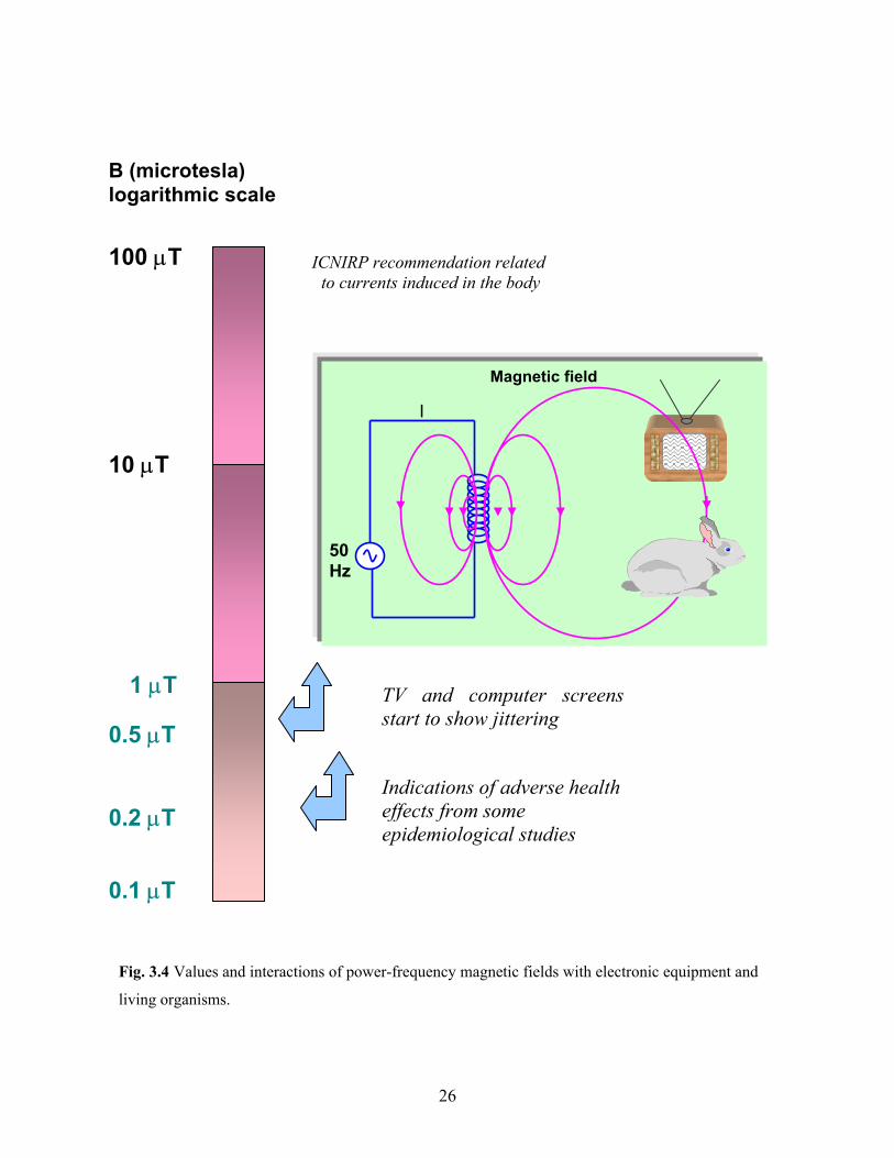
Fig. 3.4 Values and interactions of power-frequency magnetic fields with electronic equipment and
living organisms.
ICNIRP recommendation related to currents induced in the body
TV and computer screens start to show jittering
Indications of adverse health effects from some epidemiological studies
0.1 µT
100 µT
10 µT
0.5 µT
0.2 µT
1 µT
26
The fact that interference of PFMFs with electronic equipment and
suspected biological effects fall both within the same range of values
(Fig. 3.4) allows to put forward the following “working principle”[7]:
The maximum rms-values of PFMFs (in areas of residence, places where
people are staying extended periods of time, or sensitive equipment is
located) should be kept at the sub-microtesla level.
References [1] C. J. Portier, M. S. Wolfe, Eds. “Assessment of Health Effects from Exposure to Power-Line Frequency Electric and Magnetic Fields”, NIH Publication No. 98-3981, North Carolina (1998). [2] M. Feychting, and A. Ahlbom, Magnetic Fields and Cancer in People Residing Near Swedish High Voltage Power Lines, IMM-rapport 6/92, Institutet för miljömedicin, Karolinska Institutet, Stockholm, 1992. [3] IARC, Static and Extremely Low Frequency Electric and magnetic Fields, Monograms on the Evaluation of the Carcinogenic Risk in Humans, Vol. 80, Lyon, 2001. [4] M. Sandström, K. Hansson Mild, and A Berglund, “Induced Jitter on VDT Screens from external 50/60 Hz Magnetic Fields”, in Abstract book work with display units, Tech. Univ. Berlin, Sept. 1992, pp. C5-7. [5] ICNIRP (International Committee on Non-Ionizing Radiation Protection), Guidelines for limiting exposure to time-varying electric, magnetic and electromagnetic fields (up to 300 Hz), Health Physics, Vol 74, Number 4, 1988.
27

28
[6] The Swedish: National Board of Occupational Safety and Health, National Board of Housing, Building and Planning, National Electrical Safety Board, National Board of Health and Welfare, Radiation Protection Institute, Low-Frequency Electrical and Magnetic Fields: “The Precautionary Principle for National Authorities”, Solna, Sweden, 1996. [7] E. Salinas, J. Daalder, and Y. Hamnerius in: Proceedings of the CIRED-99 Conference on Electricity Distribution, Special Reports, Nice, 1999, pp. 208-209.

4 Visualization of mitigation methods
o mitigate power-frequency magnetic fields some properties of
electromagnetism and its interaction with matter can be used – resulting
in different solutions to mitigate these fields. In this report the following
methods are discussed:
T
• Conductive shielding
• Ferromagnetic shielding
• Passive compensation
• Active compensation
• Design modification of electrical facilities and equipment
In order to visualize these methods it is worth to notice that magnetic
fields with extremely low frequency (e.g. 50 Hz) can also be obtained by
rotating a permanent magnet. In fact a power frequency is not difficult to
achieve mechanically (Fig. 4.1) by means of an appropriate combination
50 Hz1 turn per second
Fig 4.1 Mechanical generation and measurement of 50 Hz magnetic fields.
29

of gears. The field is measured with a coil and an oscilloscope. Although
this way of generating a magnetic field with extremely low frequency
differs from the sources described in chapter 2, it can provide a helpful
insight on mitigation methods.
When a plate made of ferromagnetic material (with high relative perme-
ability) is placed between the magnet and the coil, the magnetic field
lines are attracted to the plate and the field diminishes. Fig. 4.2 shows a
contour plot of the magnetic field strength where field reduction is at-
tained at the other side of the plate. For example, at 20 cm from the
source, on the side containing the plate, the field is reduced by a factor of
5 compared to the value at the same distance on the opposite side.
20 cm 20 cm
× 2.5 µT
× 0.5 µT
Fig. 4.2 Magnetic field mitigation using a plate made of ferromagnetic material.
30

Another way to reduce the field of a rotating magnet1 is to place a con-
ductive plate (e.g. made of aluminum or copper) in front of the magnet.
According to Faraday’s law a varying magnetic flux induces eddy cur-
rents, mainly on the surface of the plate (Fig. 4.3-a). The direction of
a)
Fig. 4.3 Magnetic field mitigation using a plate made of conductive material.
these currents changes. When the magnet’s north-pole approaches the
plate, the flux through it increases and the induced currents on the surface
create a magnetic flux that counteracts the incident one (Fig. 4.3-b).
When it passes closest to the plate two loops are formed –this happens
1 It should be pointed out that to develop these analogies and the properties discussed here, small-scale experiments were carried out using actual rotating magnets and electronic meas-uring devices. However the contour plots and field values in figures 4.2 and 4.3 were ob-tained by modeling the shielding of a dipolar field of a solenoid at 50 Hz. These plots do not accurately represent the field of a rotating magnet and are used only for illustration purposes.
31

because on the plate there is a region where the flux increases and an-
other region where the flux diminishes. When the north-pole leaves the
plate (Fig. 4.3-c) the currents are opposite to the case (b). Conversely,
when the magnet’s south-pole approaches, reaches its maximum or
moves away from the plate, eddy currents are shifted towards 0°, as the
currents try to increase the diminishing magnetic flux (Fig. 4.3-c). An
analogous situation occurs when the magnet’s south pole approaches and
moves away from the plate (Fig. 4.3 - d, e). The net time-averaged effect
is a reduction of the field that is shown as a contour plot in Fig. 4.3-a. As
in the ferromagnetic case, the reduction is more evident on the other side
of the shield even though the field is globally affected.
It is important to note, especially in practical applications, that the conti-
nuity of the shielding plate is crucial. Any cuts, openings, holes, slits or
32Fig. 4.4 Experiment to show the efficiency of induced currents generation in a continuous conductive plate compared with a non-continuous plate.

even cracks may drastically reduce the shielding effect, as the induced
current paths will be obstructed. This can be illustrated in the experiment
shown in Fig. 4.4. Two parallel pendulums, one containing a solid copper
plate and the other containing a plate of the same material and dimen-
sions but with several slits. They oscillate in the field of two permanent
magnets with a frequency of the order of 1 Hz, leading to the formation
of eddy currents (the interaction between plates is negligible). The result
of this experiment is that the pendulum with the continuous plate slows
down very quickly and stops its oscillation (after a few seconds) while
the pendulum with the non-continuous plate continues oscillating for a
much longer time until friction forces slows it down [1]. This experiment
illustrates that the slits made on the copper plate prevent the formation of
efficient loops of eddy currents.
The generation of eddy currents on conductive plates suggests the next
two ways of mitigating magnetic fields, namely, passive and active com-
pensation. If an “imitation” of the main current loops formed in the
shielding plate is made by constructing closed copper rings and placing
them –in the same location– instead of the plate (Fig. 4.5), then field
mitigation is expected due to the generation of induction currents in the
wire loops. Compensating passive coils
Fig 4.5 The principle of passive compensation: copper loops are placed in front of the rotat-ing magnet as to “imitate” the paths of the induced currents.
33

It is also possible to cancel the field of the rotating magnet in a specific
region completely by the use of a coil carrying a current fed by a control
system (Fig. 4.6). A small coil acts as a sensor and is placed in the region
of interest. The detected signal is amplified and phase shifted electroni-
cally providing an accurate cancellation current.
Area of interest
Compensat-ing circuit
Measuring coil
Compensating coil Compensat-
ing field
Field of the magnet
Fig. 4.6 Field mitigation by active compensation: the compensating coil produces a field that cancels, in the area of interest, the original field of the rotating magnet.
The modification of the design of the rotating magnet can yield other op-
tions of field mitigation in a desired region. An example of this is the
change of the rotation axis to obtain a different geometrical configuration
of the field in the area of interest. A rotation around a horizontal axis is
shown in Fig. 4.7, the signal is (for small distances to the magnet) drasti-
34

cally damped near the axis, as there is little variation of the magnetic flux
trough the measuring coil. The global field is of the same size as before.
Fig 4.7. Modification of the design to produce a rotation around a horizontal axes; it pro-vides a different, much lower, signal on the oscilloscope; therefore a drastic mitigation of the magnetic field is achieved in the region where the coil is located.
In this chapter PFMFs mitigation techniques have been discussed.
Shielding by ferromagnetic material is yet rather effective when the fre-
quency of the rotating magnet decreases (f < 50 Hz) or even when it
stops (f = 0) creating a static magnetic field. On the other hand, shielding
by conductive materials does not work unless the magnet is moving in
such a way as to produce a time-varying magnetic flux through the
shielding surface (∆φ/∆t ≠ 0). The later can also be said about passive
compensation, since the idea is based on conductive shielding. Active
compensation works for static fields provided the system can measure
these fields.
It can also be observed that in the case of the rotating magnet the mitigat-
ing actions can affect directly the way the original field is created. For
35

36
example, in conductive shielding the eddy currents generated in the plate
do not only try to cancel the field. They also exert a braking torque on the
dipole generating the field e.g. in Fig. 4.1. To various extents similar
conclusions can be drawn for the other methods as well. This observation
illustrates that the mitigation methods could influence the operation of
the source. It is generally essential to ensure that this influence is negligi-
ble (e.g. avoiding too high mutual inductances in passive compensation)
when designing practical applications.
References
[1] R. P. Feynman, M. L. Sands, R. B. Leighton. “The Feynman Lectures on Physics” (Vol. II), Addison Wesley, Reading (1964).
[2] M. McCaig, “Permanent Magnets in Theory and Practice”, Pentech Press, London (1977).

5 PFMFs originating from secondary substations
––––––––––––––––––––––––––––––––––––––––
uring the last decade both research and the public media have
focused on the significance of magnetic fields of power transmission
lines [1-2]. However, the final distribution stage of the electrical energy
flow before reaching the customer, in particular secondary substations1,
is often a source of similar field values (in areas of concern) as
encountered at the transmission stage. This prevails in spite of the fact
that secondary substations and power lines have very different voltage
ranges (Fig. 1). On one hand, as the electric energy flows from high
voltage stages to lower ones, the current branches. Therefore, if this were
the only cause, lower magnetic fields would be expected at the end of the
electric flow. On the other hand, when the voltage diminishes (via
D
0.4 kV
0.4 kV 0.4 kV
10 kV 11-25 kV 400 kV 400 kV 130 kV
GENERATION TRANSMISSION DISTRIBUTION Loads
Loads
Loads
Fig. 5.1 A simplified diagram of the electrical energy flow from the generation plant to the customer.
1A substation is called secondary when they convert electrical energy at primary distribution voltage levels (e.g. 35 kV, 21 kV, 12.5 kV, 10 kV, or 4.16 kV) to utilization or secondary levels (e.g. 460 V, 400 V, 240 V, 208 V, or 120 V).
37

transformer operation) the current increases [3]. In addition, the distance
from sources to affected areas diminishes and the density of population
and equipment (sensitive to PFMFs) increases.
Consequently the issue of PFMFs can be considered at least as important
in highly populated neighbourhoods, such as in a city environment, as in
areas along power lines. Accordingly, the mitigation of fields from
secondary substations can contribute to the solution of some of the issues
studied in chapter 3.
5.1 In-house secondary substations In Sweden and other European countries it is not unusual, especially in
neighbourhoods with a dense population, to situate secondary substations
inside buildings. Common locations are cellars. In other countries (e.g. in
USA) the use of pad-mounted transformers is more common. These
transformers are inside a metal enclosure and placed on the ground.
Hence they are rather visible. Fig 5.2 shows a characteristic situation
displaying the sources and some typical field values. The substations
analysed in this report contain three-phase transformers (10/0.4 kV, 800
kVA). They also contain high and low voltage switchboards that have
covers customarily made of plane steel and they both enclose busbars.
However, due to the reduction in voltage, the currents increase with the
same factor at the secondary side of the transformers. Therefore cables,
and busbars at the low voltage part of the substation constitute major
sources of magnetic fields. Hence methods to mitigate their fields will be
the goal of the next chapters.
38

Cables
4.4 µT
20 µT
1.6 µT
2.5 µT
33 µT
10 µT
Switchboard and busbars
Three-phase transformer
1m
4m
1.1 µT
Fig. 5.2 Some typical magnetic field values (in microtesla) from a secondary substation situated in a cellar of a building. A usual configuration of major sources and distances is also shown.
The magnetic field values originated from a secondary substation are the
result of an intricate superposition of the fields from various sources. It is
39

then natural to ask: is it possible to discriminate in advance the
magnitude of the contribution of each source by scanning the field values
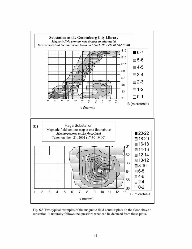
in the affected area (Fig. 5.3)? The answer –as we will learn in the next
chapters– is yes. There are two reasons for this: (1) Analysis of the field
gradient on the scanned surface could suggest the possible source
behaviour. (2) Analysis of the variation of the field values with the
distance perpendicular to the scanned surface could provide a 3
dimensional picture of the field decay, and subsequent source
identification. Moreover, after a simple inspection of the substation itself
(this may include a few extra measurements), the problem can be
straightened out, and a mitigation method can be suggested. See
applications of these techniques in chapters 11 and 12.
References
[1] M. Feychting and A. Ahlbom, “Magnetic Fields and Cancer in People Residing Near Swedish High Voltage Power Lines”, IMM-rapport 6/92, Institutet för Miljömedicin, Karolinska institutet, Stockholm, 1992. [2] G. Theriault et al: ”Risk of leukemia among residents close to high voltage transmission electric lines” Occup Environ Med 54: 625-628, 1997. [3] T. Wildi, “Electrical Machines Drives and Power Systems”, Second edition, Prentice-Hall International, London, 1991.
40
1 2 3 4 5 6 7 8 9 10 11 12 13
S1
S2
S3
S4
S5
S6
20-2218-2016-1814-1612-1410-128-106-84-62-40-2
1 3 5 7 9 11 13 15 17 19 21
S1
S3
S5
S7
S9
S11
S13
S15
Y
6-7
5-64-5
3-42-3
1-20-1
Substation at the Gothenburg City Library Magnetic field contour map (values in microtesla)
Measurements at the floor level, taken on March 20, 1997 (8:00-10:00)
x (metres)
B (microtesla) Xx (metres)
(b) Haga Substation Magnetic field contour map at one floor above
Measurements at the floor level Taken on Nov. 21, 2001 (17:30-19:00)
B (microtesla)
Fig. 5.3 Two typical examples of the magnetic field contour plots on the floor above a substation. It naturally follows the question: what can be deduced from these plots?
41

42

6 Phase arrangements ––––––––––––––––––––––––––––––––––––––––
ables, wires, power lines and busbars are the carriers of electrical
C
energy and sources of PFMFs. Hence, the phase configuration andgeometrical positioning of these sources are essential factors in the
design of electrical installations with low PFMFs. This is, nevertheless,
also valid for old installations. If the initial design did not consider
optimal cable arrangements, a set of suitable modifications can yet be
made which leads to mitigation of PFMFs.
Here we will give examples of the field around given phase
configurations assuming the following: (1) The relative permeability of
the surrounding environment is unity, and (2) the conductivity of the
surrounding material is zero. The computations are based on direct
application of the formulas given in chapter 2 (for instance Eq. 2.10). The
field can be obtained analytically (for simple geometries) or, in general,
by numerical techniques such as FEM codes. The latter is the method
applied in this chapter. The FEM solver code ELEKTRA was used [1],
which has the grid generator OPERA 2D/3D. ELEKTRA evaluates the
field from a conductor of nearly any shape by integrating the Biot-Savart
formula. Current densities and dimensions of conductors are the main
inputs. To enable these conductors to be oriented in space correctly, local
coordinate systems can be used. To reduce the amount of input data when
dealing with several conductors, operations such as reflections and
translations can be used to replicate any basic shape.
43

The computation that follows is an example of how phase arrangement
can be used as a field mitigation technique.
6.1 PFMFs from bundles of three-phase conductors Three bundles of three-phase conductors R (0º), S (120º) and T (240º)
carrying a 50 Hz current of 100A (rms) are grouped in different phase
arrangements as shown in Fig. 6.1. The aim is to find the arrangement,
x
y
R
T S
S
T R
T
R S
S
T R
S
T R
S
T R
R
R R
S
S S
T
T T
R
T S
S
R T
T
S R Different phases arrangement 3
Different phases arrangement 2
Different phases arrangement 1
Equal phases arrangement
0.04 m0.04 m
Fig. 6.1 Different phase arrangements for a system of nine conductors, each conductor diameter is 0.02 m, insulation thickness 0.01 m, and the current per phase is I = 100A.
44

which provides the lowest values of PFMF at a certain distance (y) larger
than the cross-sectional dimensions of the arrangement (~ 0.2 m).
The results are presented in Fig. 6.2. The contour plots are all on the
same scale, the field values are plotted within the range [0.1 – 1] µT, and
the interval between lines is 0.05 µT. It can be observed that the
arrangement number 3 of bundles with different phases has the lowest
field emission.
1µT 0.1µT
Equal phases
Arrangement 3 Arrangement 2
Arrangement 1
Fig. 6.2 Contour plots for the different phase configurations of Fig. 6.1. The plots are all on the same scale, the field values are plotted within the range [0.1 - 1] µT, and the interval between lines is 0.05 µT. The axis scales are in metres.
45
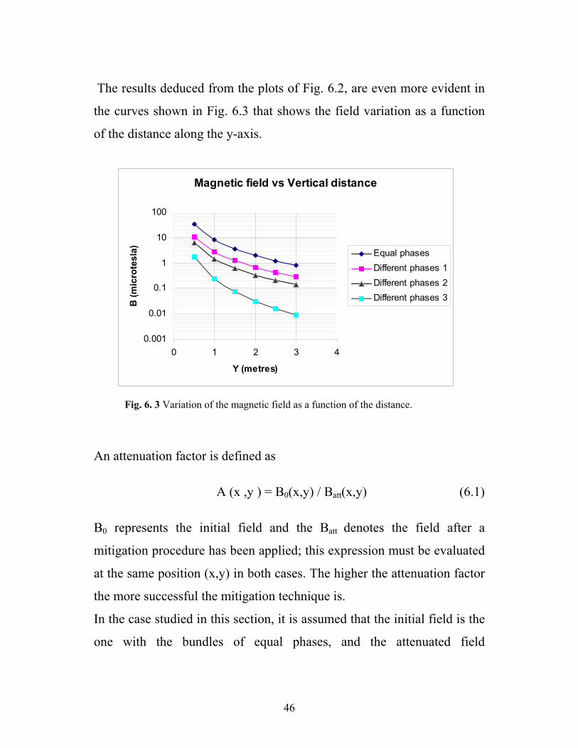
The results deduced from the plots of Fig. 6.2, are even more evident in
the curves shown in Fig. 6.3 that shows the field variation as a function
of the distance along the y-axis.
Magnetic field vs Vertical distance
0.001
0.01
0.1
1
10
100
0 1 2 3 4
Y (metres)
B (m
icro
tesl
a) Equal phasesDifferent phases 1Different phases 2Different phases 3
Fig. 6. 3 Variation of the magnetic field as a function of the distance.
An attenuation factor is defined as
A (x ,y ) = B0(x,y) / Batt(x,y) (6.1)
B0 represents the initial field and the Batt denotes the field after a
mitigation procedure has been applied; this expression must be evaluated
at the same position (x,y) in both cases. The higher the attenuation factor
the more successful the mitigation technique is.
In the case studied in this section, it is assumed that the initial field is the
one with the bundles of equal phases, and the attenuated field
46

corresponds to the various cases of combining phases in different
bundles. Applying this definition to the values of the different phase
arrangements we obtain the following table:
Table 6.1 Field of equal phases and attenuation factors (B0 / Batt) of various arrangements
y = 0.5 m y = 1 m y = 1.5 m y = 2 m y = 2.5 m y = 3 m
Field B0 (equal phases) 33.70 µT 8.27 µT 3.58 µT 1.95 µT 1.20 µT 0.80 µT
Different phases, A1 3.11 3.0 2.93 2.87 2.79 2.67
Different phases, A2 5.48 5.75 5.83 5.87 5.89 5.9
Different phases, A3 19.2 34.5 49.4 63.4 76.5 88.9
Analysing the variation of the attenuation factors with distance, given in
table 6.1, one can see that: the attenuation diminishes for the
arrangements 1 whereas it increases for arrangements 2 and 3. That is to
say, the latter arrangements (especially arrangement 3) not only provide
better mitigation than the first one, but it also improves with the distance
– at least in the areas of interest. This property can be very useful since
often the interest is to mitigate an affected area which distance from the
source is large in comparison with the dimensions of the source.
Three dimensional arrangements with variation in the z direction can also
be taken into account. This allows further mitigation by the operation of
twisting the conductors. In this way there is a partial cancellation of some
of the contribution to the field integration along the z - direction. This
action is, however, not always possible, especially for high current
conductors, due to the stiffness of the conductors.
The method presented in this chapter, and considerations of heat
conduction, can be readily applied to arrangements of underground
47
cables [2], power lines, connections between the low-voltage side of a
substation transformer (Section 11.2) and a switchboard and, in general,
to any electrical installation where a field source of high magnetic fields
is located in inadequately designed groupings of cables or wires.
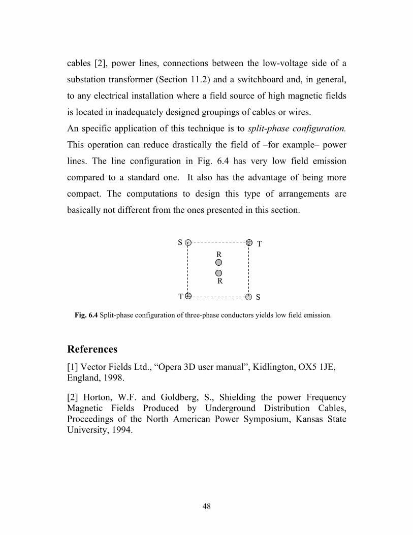
An specific application of this technique is to split-phase configuration.
This operation can reduce drastically the field of –for example– power
lines. The line configuration in Fig. 6.4 has very low field emission
compared to a standard one. It also has the advantage of being more
compact. The computations to design this type of arrangements are
basically not different from the ones presented in this section.
T
R
R S T
S
Fig. 6.4 Split-phase configuration of three-phase conductors yields low field emission.
References [1] Vector Fields Ltd., “Opera 3D user manual”, Kidlington, OX5 1JE, England, 1998. [2] Horton, W.F. and Goldberg, S., Shielding the power Frequency Magnetic Fields Produced by Underground Distribution Cables, Proceedings of the North American Power Symposium, Kansas State University, 1994.
48

7 Modelling PFMFs using 2D and 3D FEM codes
––––––––––––––––––––––––––––––––––––––––
he behaviour of power devices such as transformers, electrical
machines or power lines is governed by electromagnetic fields that obey
the Maxwell equations. Consequently, in order to predict the behaviour
of these devices (e.g. in the course of their design or in a field mitigation
problem) one must solve Maxwell’s equations. This involves dealing
with a set of differential equations and adequate boundary conditions.
Analytical methods [1] (e.g. separation of variables, Laplace
transformations or series expansions) cover only a very few cases which
involve a high degree of symmetry. Numerical methods are necessary to
solve these equations more generally.
T
The method of finite differences [2] has been rather popular since the
very origin of computational electromagnetics. It subdivides the solution
region into a rectangular grid or a mesh of points. This method
transforms the complicated problem of dealing with differential
equations to an approximately equivalent and much easier one: a set of
linear algebraic equations. A drawback of this method is its poor
flexibility when dealing with oblique and curved boundaries.
As computer capabilities increased other computational methods were
developed [2], [3], integral equation formulations [4], often referred as
the method of moments (MoM) for which several different formulations
exist [5]. However, the method that is nowadays widely accepted as a
49
powerful technique in electrical engineering problems is the finite
element method (FEM) [3], [7]. This chapter will focus on this particular
technique.
7.1 Quasi-static electromagnetic fields When the wavelength of a time-varying field is much larger than the
dimensions of the problem (i.e. in the near field zone), then the set of
four Maxwell equations simplify. One reason for this is that the
displacement current term becomes negligible in comparison with the
current density J. Thus the Ampère law is a good approximation for
Ampère-Maxwell equation. The set of equations given in Eq. 7.1 (a)
describes electromagnetic phenomena in a quasi-static regime.
The low frequency approximation formally amounts to setting ε0 = 0 ;
therefore the fourth equation in Eq. 7.1 (a) is also disregarded. In fact, in
any modelling of eddy currents only three of the Maxwell equations are
involved [6]. Moreover, in this report, the fields have sinusoidal
variation, thus one can use the complex formulation of the fields: E (t)=
Re{ exp(jωt)}, and H (t)= Re{ exp(jωt)}, where j is the imaginary
unit, and ω is the angular frequency. Consequently, for modelling PFMFs
in a medium containing regions with σ and µ, (for example shielding of
power sources using ferromagnetic or conductive material) Maxwell’s
equations simplify ending to the set given by Eq. 7.1(b).
E H
The following additional assumptions are often made in modelling a
PFMFs mitigation problem:
(1) The conducting media are linear with respect to the current.
50

(2) The conducting media are isotropic.
(3) The relative permeability µr of the conductive media is constant.
(4) A macroscopic model is used for the conducting media.
(5) Thermal effects are neglected or considered linear.
It should be noted that current research in electromagnetic modelling is
concerned with removing most of these assumptions. An example is the
inclusion of realistic permeability curves in recent models.
ρ=⋅∇=⋅∇
∂∂
−=×∇
=×∇
DB
BE
JH
0t
( ) sj
s
JEHHEJEH
⋅∇=⋅∇=⋅∇−=×∇
+=×∇
)(,0 σµωµ
σ
EJEDHB
σµµ
===
Equations for electromagnetic modelling
Ampere Law Faraday Law Gauss law for B Gauss law for E Constitutive relation Constitutive relation
Ohm’s law
Eq. 7.1 (a) Quasi-static fields
Eq. 7.1 (b) Eddy current formulation for PFMFs
7.2 The finite elements method (FEM) This method is increasingly popular [7], [8] due to its ability to deal with
regions with very complex geometries. It divides the region under study
into a number of sub-domains (usually triangles, quadrilaterals,
51
tetrahedra, or hexahedra) called elements. The field on each element is
approximated by a simple algebraic expression; hence the values of the
field on a finite set of nodal points or edges are determined as the
solution of a linear set of equations. To deal with an unbounded
geometry, several approaches are possible. Boundary elements can
accurately model an infinite region, however reasonable approximation
can be found using differential equation solvers by surrounding the
region of interest by a large box. The accuracy of the solution depends,
among other factors, on the size of the limiting box (or external
boundary) and the number and distribution of elements. Two commercial
codes have been extensively used in the present work: 2D ACE from
ABB Research Corporation [9], and 3D ELEKTRA from the company
Vector Fields [10]. Both use the method of a large surrounding box.
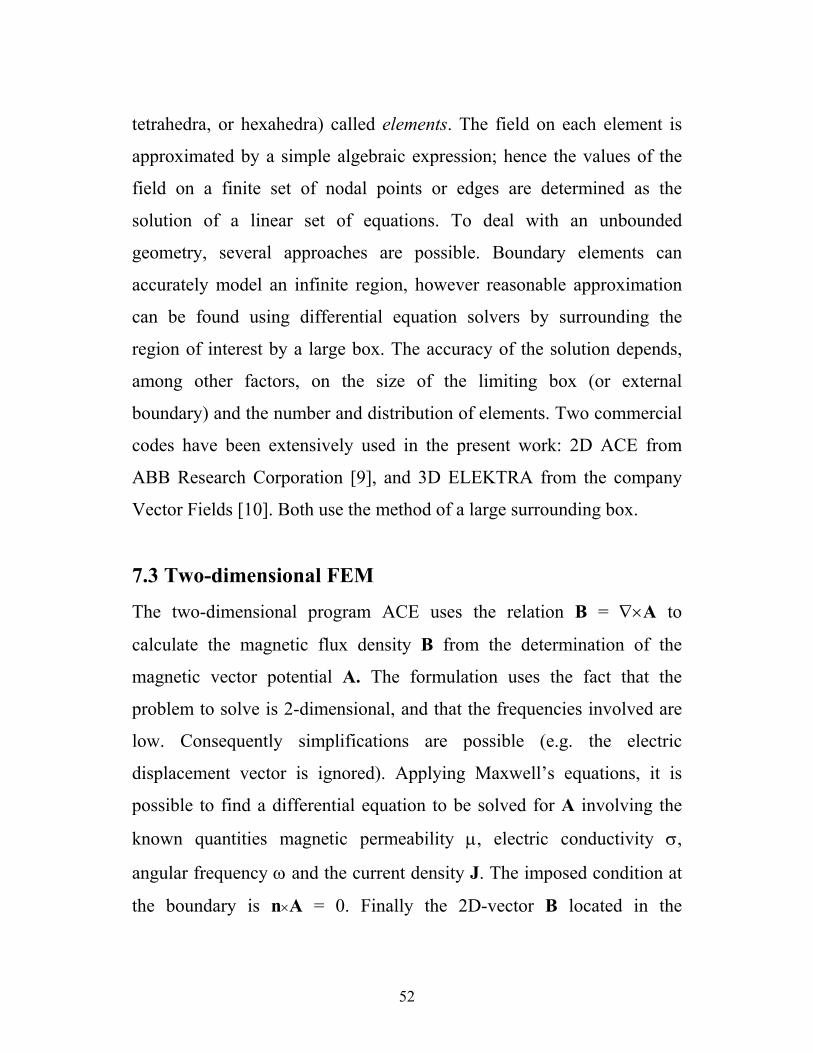
7.3 Two-dimensional FEM
The two-dimensional program ACE uses the relation B = ∇×A to
calculate the magnetic flux density B from the determination of the
magnetic vector potential A. The formulation uses the fact that the
problem to solve is 2-dimensional, and that the frequencies involved are
low. Consequently simplifications are possible (e.g. the electric
displacement vector is ignored). Applying Maxwell’s equations, it is
possible to find a differential equation to be solved for A involving the
known quantities magnetic permeability µ, electric conductivity σ,
angular frequency ω and the current density J. The imposed condition at
the boundary is n×A = 0. Finally the 2D-vector B located in the
52
symmetry plane is determined. A good characteristic of the ACE
program is that its mesh generator is adaptive, making it possible to run
different variations of the geometry of a problem, without having to
spend too much time on mesh generation.
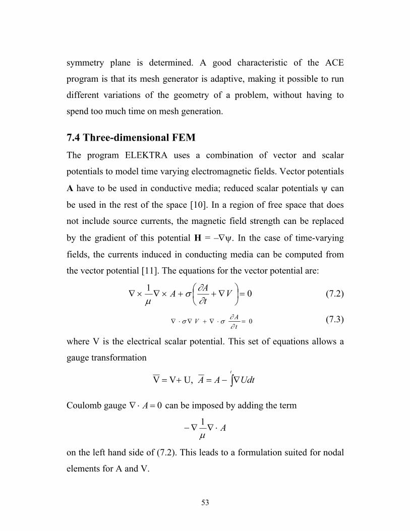
7.4 Three-dimensional FEM The program ELEKTRA uses a combination of vector and scalar
potentials to model time varying electromagnetic fields. Vector potentials
A have to be used in conductive media; reduced scalar potentials ψ can
be used in the rest of the space [10]. In a region of free space that does
not include source currents, the magnetic field strength can be replaced
by the gradient of this potential H = –∇ψ. In the case of time-varying
fields, the currents induced in conducting media can be computed from
the vector potential [11]. The equations for the vector potential are:
01=
∇++×∇×∇ V
tAA
∂∂σ
µ (7.2)
0=⋅∇+∇⋅∇tAV
∂∂σσ (7.3)
where V is the electrical scalar potential. This set of equations allows a
gauge transformation
∫∇−=+=t
UdtAAU,VV
Coulomb gauge 0=⋅∇ A can be imposed by adding the term
A⋅∇∇−µ1
on the left hand side of (7.2). This leads to a formulation suited for nodal
elements for A and V.
53

The equations are simplified and solved for A under the condition of
steady state alternating current excitation; this condition assumes linear
materials. Having determined A, the code calculates the distribution of
the magnetic flux density within the 3-dimensional domain of the
problem.
The boundary conditions are essential in the specification of the problem
to be modelled. They can be applied in two situations:
(1) To reduce the size of the geometry of the problem by symmetry.
(2) To approximate the magnetic field at large distances.
The boundary condition used in the far-field boundaries of the problems
in this report is TANGENTIAL MAGNETIC, i.e. H·n = 0, and 0=∂∂
nψ ,
where n is the normal unit vector to the surface being considered and ψ
represents either the reduced or the total scalar potential.
One difficulty with the Vector Fields mesh generator (OPERA-3d) is the
cumbersome way the mesh has to be generated. This makes undertaking
the modelling of a problem that requires the variation of the geometry
parameters a very time consuming task.
7.5 Modelling a mitigation problem in a 3D FEM code. There are several stages to reach the solution of a mitigation problem (or
in general of an electromagnetic problem) modelled by a FEM code. The
most relevant and useful stages are
1) Specification of the physical model: geometry, shielding materials,
conductors are given.
54

2) Reduction of the various parts to a geometrical structure. They are
embedded in a box large enough to permit the decay of the field to
negligible values.
3) Formation of the base plane or a section of it (if the problem
contains symmetries) with the help of construction lines. The
coordinate points are positioned and then facets, i.e. close squares
or polygons, are constructed.
4) Partition of the sides of the facets into a number of subdivisions,
which can be uniform or variable, i.e. more dense in certain
regions than in others according to the expected field variation.
5) Extrusion of the base plane along a direction (the z direction is
chosen in all modelling presented in this report). This action
creates various layers and generates the required geometrical
structure in the third dimension.
6) Material modification: the material properties for each layer are
named. They are said to be modified because the default is AIR,
which stands for σ = 0 and µ =1. The type of the potential is also
specified here by choosing between REDUCED (regions
containing the source conductors), TOTAL (in regions where the
mitigation is high) or VECTOR (for regions where eddy currents
are formed).
7) Setting of boundary conditions, they are specified on the external
faces.
8) Conductor specification, the conductors are defined by their
dimensions, positioning and current density and each one is given
a label.
55

9) Meshing, the program divides the problem space into elements and
positions the nodes.
10) An Analysis file is created and a data base is completed by
specifying the phases of the labels of the different conductors and
the working frequency. The conductivity, permeability and
linearity of materials is specified. Finally the file is saved ending
the pre-processing operation.
11) The solver ELEKTRA is activated. This will calculate the matrix
coefficients for one equation per node. The coefficients of the
equations are formed into a matrix. The program also calculates
the right-hand side terms of the equations and finally, by a
preconditioned iterative method, solves the equations.
12) The solution is analysed by the post-processor. In the modelling
of PFMFs the parameter BMOD evaluates the value of the
magnetic flux at phase 0º. However at 90º BMOD can have a
rather different value, and this has to be taken into account.
Therefore the following expression gives the correct rms values
#BTOT=SQRT(BMOD**2 + iBx**2 + iBy**2 + iBz**2).
13) Finally the field is evaluated and plotted. This can be done point
by point, in contour plots, or in 3D diagrams.
7.6 Modelling a 2D problem using OPERA-3d
56

The field mitigation modelling in this report is adapted to the operation
of extrusion (step 5 in section 7.5.). Moreover, it takes advantage of it by
Fig. 7.1 The 2D formulation of a shielding problem in terms of potentials for the case of three- phase underground cables.
Three-phase conductors
Wedge-shaped shield, vector potential formulation
Scalar potential formulation everywhere but in the shield
Fig. 7.2 3D approach of the 2D shielding problem. The extrusion in the z-direction has only one subdivision. This approach makes it easier to model other cases of similar cross-section but much shorter dimensions.
57

reducing the time spend in pre-processing when a large number of cases
are modelled. The most difficult part is the generation of subdivisions
and meshing on the base plane because the coordinate points. For this
reason, even if a problem can be considered as 2D (because of the
characteristics of the geometry) as in Fig. 7.1, it is still possible and
convenient to approach this as a 3D problem and making an equivalence
to a 2D problem. This is achieved by defining a second plane at a rather
large distance from the base plane (e.g. 200 metres in the case of
modelling of long cables). An extrusion with one element forming only
one layer will define an equivalent of a 2D problem (Fig. 7.2). The
solution is evaluated in a plane at the middle of the grid. The advantage
of this approach is that the grid can be kept and used again in other
problems with similar cross-sections but of much shorter length – where
edge effects become relevant. This can be attained with very little
modifications, mainly shortening the original extrusion and defining
more extrusion planes to generate the 3D grid.
References [1] Binns, K. J., and Laurenson, P.J., Analysis and Computation of Electric and Magnetic Field Problems, Pergamon Press, Oxford, 1963. [2] Booton, R. C., Computational Methods John Wiley& Sons, Inc., N.Y., 1992. [3] J. Jin, The Finite Element Method in Electromagnetics, Wiley, New York, 1993.
58

[4] Mayergoyz, I. D., “A New Approach to the calculation of Three-Dimensional Skin-Effect Problems” IEEE Trans. Magn.Vol. MAG-19, No. 5, 1983, pp. 2198-2200. [5] Harrington, R. F., Field Computation by Moment Methods, Krieger, Florida, 1987. [6] Stoll, R. L., The Analysis of eddy Currents, Claredon Press, Oxford, 1974. [7] Silvester, P. P. and Ferrari, R. L., Finite Elements for Electrical Engineers, Cambridge University Press, New York, 1983. [8] Chari, M. V. K., and Salon S. J., Numerical Methods in Electromagnetism, Academic Press, San Diego, 2000. [9] ABB Corporate Research, The ABB Common Platform for 2D Field Analysis and Simulation, Ace 2.2 User Manual, 4th Edition, Västerås, 1993. [10] Vector Fields Ltd., “Opera 3D user manual”, Kidlington, OX5 1JE, England, 1998. [11] Binns, K. J., Lawrenson, P. J., Trowbridge, C. W., The Analytical and Numerical Solution of Electric and Magnetic Fields, John Wiley & Sons, N.Y., 1994. [12] Salinas. E. “Using OPERA for passive and active shielding of 50 Hz Magnetic Fields”, Vector Fields European User Meeting 2000, Proceedings, Lille, 2000.
59

60

8 PFMFs from Busbars ––––––––––––––––––––––––––––––––––––––––
usbars are the most efficient way to transport large amounts of
electrical energy within a reduced space such as a secondary substation.
They are usually made of copper or aluminium covered by copper.
Depending on their specific design they can have different lengths,
geometrical arrangements, and cross sections. Two typical arrangements
are shown in figure 8.1. In this chapter a number of properties are
deduced of PFMFs originating from busbars.
B
Cross-sections
(a) (b)
Fig. 8.1 Two different geometrical arrangements of busbars, (a) simple and (b) complex.
61

8.1 Equivalence of busbars to a set of thin wires
In order to calculate the magnetic field of a three-phase system of
busbars it is useful to consider them as segments of infinitely thin
conductors. This approximation holds well for distances larger than the
dimensions of the system (i.e. x and y > b), which is given by the
separation b between busbars. Fig. 8.2 shows the contour plots for a
common type of a busbars system. It has the following parameters: cross-
section of each bar = (0.1 m) x (0.01 m), current per phase I = 400 A
(rms), separation between busbars b = 0.2 m, length L = 2m. The field
was evaluated for three different scales corresponding to the value
ranges: I) [500 µT- 1000 µT], II) [50 µT- 500 µT], and III) [0.5 µT- 5
µT]. There are differences in field values only in the first range. In the
areas of interest, i.e. range III, the systems are equivalent (i.e. they differ
in les than 1%). This fact makes the formulas presented in chapter 2
useful for evaluating the properties of the field from busbars.
8.2 Dependence on the length
In order to have a realistic approach, when studying the field from
busbars systems, it is important to determine when to use 2-dimensional
or 3-dimensional computational codes. For the specific case presented in
the former section, the field is evaluated on the plane with vertical
distance Z = Z1 = 4m. Fig. 8.3 shows that 2D simulations can be applied
accurately for long systems (L >> 10m). This is because the field
62
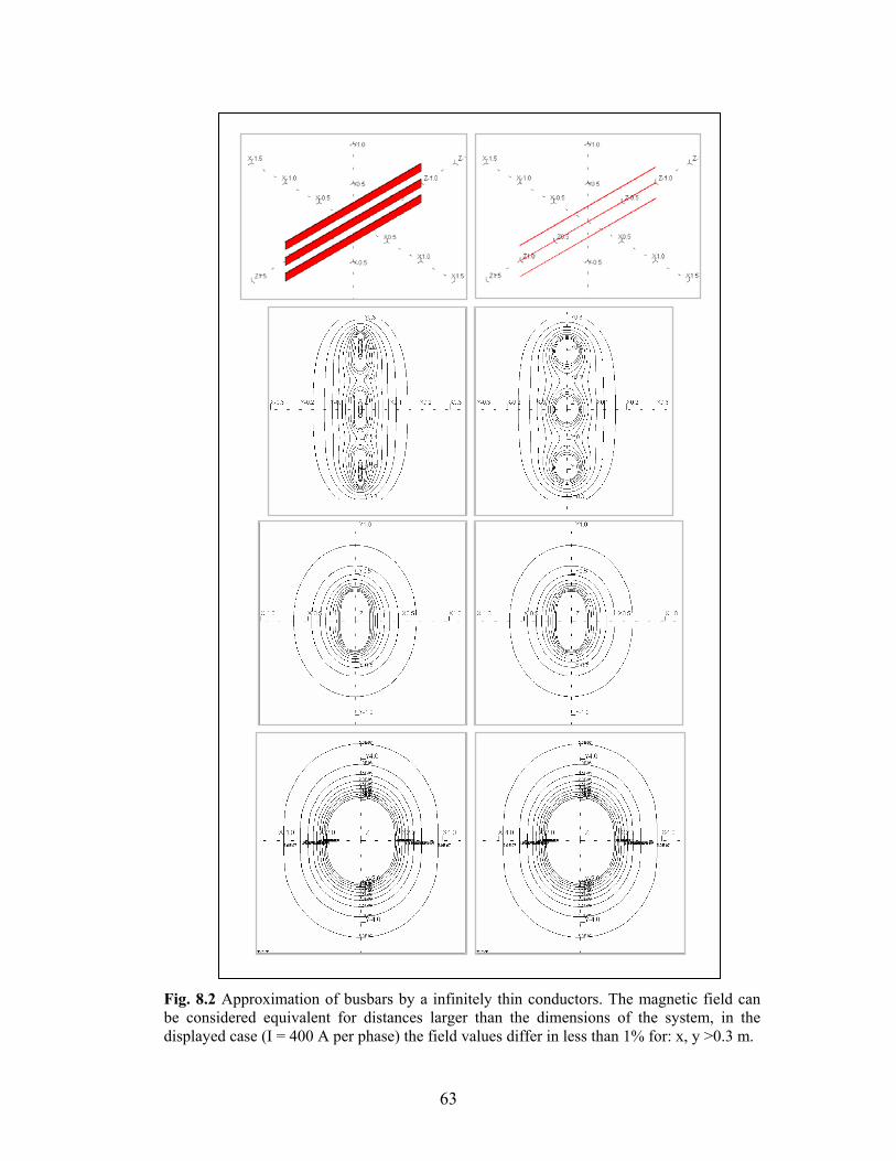
Fig. 8.2 Approximation of busbars by a infinitely thin conductors. The magnetic field can be considered equivalent for distances larger than the dimensions of the system, in the displayed case (I = 400 A per phase) the field values differ in less than 1% for: x, y >0.3 m.
63
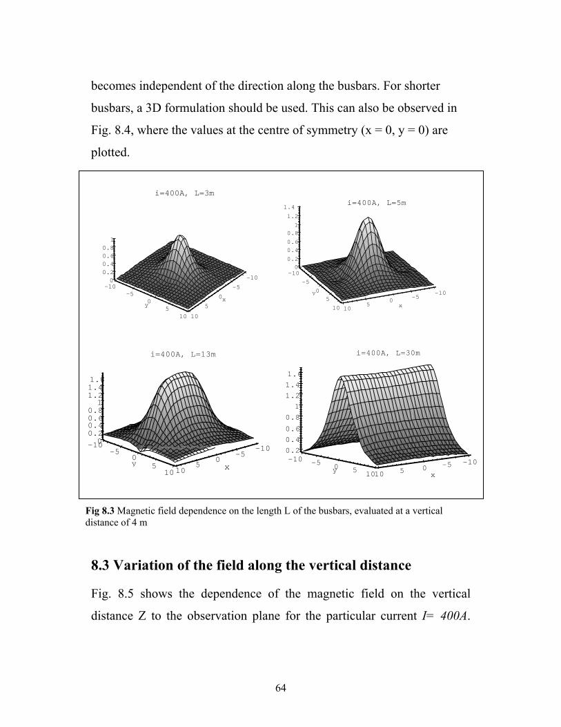
becomes independent of the direction along the busbars. For shorter
busbars, a 3D formulation should be used. This can also be observed in
Fig. 8.4, where the values at the centre of symmetry (x = 0, y = 0) are
plotted.
1 0.8 0.6 0.4 0.2 0
y 10
5 0
-5 -10
x
10 5
0 -5
-10
i=400A, L=3m 1.4
1.2
1
0.8
0.6
0.4
0.2
0
y
10
5
0
-5
-10
x 105
0-5 -10
i=400A, L=5m
1.6
1.4
1.2
1
0.8
0.6
0.4
0.2
y 1050-5-10
x 10 5 0 -5 -10
i=400A, L=30m
1.6 1.4 1.2 1
0.8 0.6 0.4 0.2 0
y 10 5
0 -5 -10
x10 5 0 -5-10
i=400A, L=13m
Fig 8.3 Magnetic field dependence on the length L of the busbars, evaluated at a vertical distance of 4 m
8.3 Variation of the field along the vertical distance Fig. 8.5 shows the dependence of the magnetic field on the vertical
distance Z to the observation plane for the particular current I= 400A.
64

The separation between busbars is b = 0.2 m. This dependence is shown
for various lengths of the busbars system.
L (m)
5040302010 0
1.6
1.4 1.2 1
0.8 0.6 0.4 0.2
0
B (x=0,y=0, Z=4m) vs L
B (L → ∞)
Fig. 8.4 Dependence on the length L .
Z (meters) 108 6 4 2
6
5
4
3
2
1
0
B (at x=0,y=0)vs Z
I=400A
B (microtesla)
L =8m L =13m
L =30m
L =1m L =2m
L =4m
Fig. 8.5 Variation of the magnetic field as a function of the vertical distance from the busbars system to the measuring point.
65

8.4 Field variation with the distance between busbars In a similar way as the study for bundles of several conductors in the
former chapter, the distance (b) between busbars is very important; the
larger it is, the higher the field will be (Fig. 8.6). When the distance is
very small, the fields from the three phases tend to cancel each other.
b (m) 10.80.60.40.2 0
2
1.5
1
0.5
0
B vs b (distance between bus bars) L=2m, Z=4m, x=0, y=0, i=400A
B(µT)
Fig. 8.6 Variation of the field as a function of the distance (b) between busbars.
It is often necessary to contrast shielding results with the case when the
shield is not present. Results discussed here become relevant in that case.
References [1] E. Salinas and L. Aspemyr, Experimental Study of 50 Hz Magnetic Fields from 10/0.4 kV Substation Components. Proceedings of the Fourth Latinamerican Congress on Electrical Genertion, Transmission and Distribution, Vinha del Mar, 2000.
[2] E. Salinas and L. Aspemyr, Measurements and Reduction of 50 Hz Magnetic Fields from the New Substation at the Department of Electric Power Engineering, Technical Report No. 14R, ISSN: 1401-6176, Chalmers University of Technology, Gothenburg, 1999.
66

9 Conductive and ferromagnetic shielding
––––––––––––––––––––––––––––––––––––––––
or the reason of cost-effectiveness the main interest in shielding
PFMFs is in thin shields. By shield we mean a finite metal layer (open,
closed or semi-closed) that is placed around or near a device (or an
affected area) whose magnetic field is aimed at mitigation. Thin refers to
sub-centimetre thickness. Most of the results in this chapter are deduced
for three-phase busbars systems. However, the method can be applied to
various sources such as coils or cable arrangements carrying mono or
multi-phase currents.
F
9.1 Shielding effectiveness at power frequencies It is customary to discuss the performance of a shield in terms of a figure
of merit named shielding effectiveness (SE). The shielding efficiency
depends on the ratio of the field evaluated at the point (x,y,z) for two
different circumstances and depends on the frequency. For quasi-static
systems (e.g. power frequency regime) the electric and magnetic fields
can be considered separately. For the magnetic field1 it is defined in
decibels (dB) as:
=
),,(),,(log20 0
10zyxB
zyxBSEShielded
(9.1)
ion is given for the shielding efficiency of electric fields in the quasi
]h
1 A similar express -static regime: . However at high frequencies E and B cannot
be considered separately, thus S has to be defined by means of t e electromagnetic power flow P(x,y,z) evaluated before and after placing the shield:
[ ),,(/),,(log20 010 zyxEzyxESE Shielded=
[ ]),,(/),,(log 010 zyxPzyxP Shielded10SE = .
67

where B0 is the magnetic field in the absence of the shield, and BShielded is
the magnetic field after placing the shield.
Unlike the case of high frequencies [1], where mitigation of several
orders of magnitude can be rather common, a field reduction of an order
of magnitude at power frequencies is often considered rather good. In
this case the definition of the attenuation factor A given in chapter 6 can
still be used in practical evaluations of shielding.
9.2 Penetration depth
When a harmonically varying magnetic field t)(x,B ω penetrates a
metallic medium with conductivity σ, and permeability µ, the magnetic
flux change produces an electromotive force (EMF), which induces eddy
currents circulating in the conductor and opposing the incident field. As a
result of this the net magnetic field is altered. This is a situation that can
be solved exactly using Maxwell’s equations for the quasi-static regime.
In fact, the problem is fully 1-dimensional, even though three dimensions
are involved! (i.e. the fields B and H have only one component along the
vertical direction y, the eddy currents and the associated electric field
propagate along z, yet these four quantities vary only in the direction x).
In Fig. 9.1, since 0/ =∂∂ y , and 0/ =∂∂ z , the set of equations given in
Eq. 7.1-(a)-(b) simplify. Thus Faraday’s law that governs eddy currents
becomes:
BjxJ ω
σ=
∂∂1 (9.2)
68

At the same time, these currents generate a magnetic field, this is
described by Ampere’s law
JxH
=∂∂ (9.3)
Fig. 9.1 Propagation of a magnetic field inside a semi-infinite medium.
J ●
µ, σ
x B
These two equations, and the constitutive relation HB µ= , give a second
order differential equation:
02
2
=−∂∂ Bj
xB ωµσ (9.4)
to which the general solution is
)exp()exp( 21 xjCxjCB ωµσωµσ −+= (9.5)
Applying the boundary condition 0)( =∞→xB makes C1 to vanish.
Defining the field at the surface of the interface as 02)0( BCxB ≡== ,
and introducing the penetration depth (or skin depth) δ which is defined
as
ωµσδ 2= (9.6)
69

Then the solution becomes
δxj
eBB)1(
0+−
= (9.7)
Thus the magnetic field is both damped and phase shifted with distance
inside the conductor. A similar behaviour is obtained for the current
density J. Eq. (9.2) together with Eq. (9.7) gives
δ
µδ
xjejBJ
)1(0
)1( +−+−= (9.8)
Defining µδ)1(00 jBJ += as the current density at the surface,
δxj
eJJ)1(
0+−
= (9.9)
Consequently the current density also decays inside the material in the
same fashion than the magnetic flux density B.
Table 9.1 shows the penetration depth calculated for some common
metals. Table 9.1
Penetration depth δ [mm]
f (Hz)
Cu σ = 5.99 x10⁷Sm-1
Al
σ = 3.77x10⁷Sm-1
Fe
µr=200
25 13.4 17.4 2.54
50 9.44 12.3 1.8
100 6.77 8.7 1.3
1 000 2.11 2.75 0.41
10 000 0.667 0.87 0.13
100 000 0.211 2.75 0.041
1 000 000 0.067 0.087 0.13
70

71
The penetration depth in iron is much smaller than that of aluminium or
copper. Therefore, it is common [2] to regard conductive shielding with
thin non-magnetic materials at power frequencies as inherently
inefficient (since any practical shield would have thickness < δ), or, in
any case not better than iron. However, the problem is not settled by the
concept of penetration depth, since the model presented in this section
contains various ideal assumptions. In the EMC literature [3], [4], other
models for thin layers have been developed but it is still common to
consider infinite dimensions in the direction perpendicular to the plate,
which enables to study the model analytically. Another assumption is to
develop the model for high frequencies where the electric and magnetic
fields are coupled and form a plane wave, which is not the case of
PFMFs
9.3 Modelling of finite and open shields
The complexity of shielding PFMFs with thin finite plates is shown in
Fig 9.2 for a three-phase system of busbars. The incident field
experiences reflection, penetration and diffraction around the borders of
the shield. Moreover inside the shield reflection on the second surface
becomes relevant when the shield is thin, in addition power absorption
due to ohmic losses (which are temperature dependent) take place. As a
result of this, an accurate study of finite, open shields by analytical
methods is difficult and to obtain accurate numbers numerical modelling
is required.
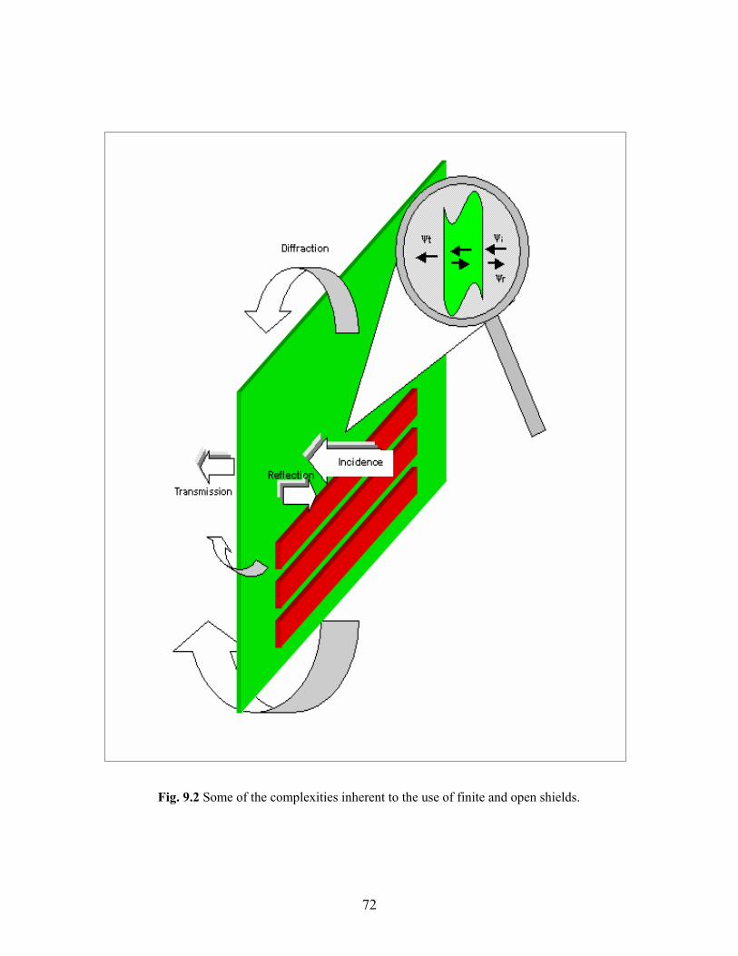
Fig. 9.2 Some of the complexities inherent to the use of finite and open shields.
72

Figures 9.3 and 9.4 show two examples of geometrical configuration for
the OPERA-3d pre-processing of simulations with busbars and coils.
Coils have different field patterns thus yield extra information to the
shielding analysis. The shield with dimensions 2m x 1m is divided in
Fig. 9.3 Pre-processing geometrical configuration for the shielding of a 3-phase busbars system (L = 2m). The plate thickness is 3 mm and the distance d plate to busbars is 20 cm. The current in the busbars is 100 A per phase.
Fig 9.4 Shielding of the magnetic field of a coil. The size of the plate is 2 m wide, 1 m high, and 5 mm thick.
73

facets, next it is subdivided even further by allocating enough number of
elements along the plate thickness to permit assessment of eddy currents
(Fig. 9.5).
Base plane
Source
Shield
Mesh around the shield
Shield
Fig. 9.5. Construction of a mesh for the shielding configurations described in Fig. 9.3, and 9.4.
74

The structure of the mesh in Fig. 9.5 contains 52 000 elements. and the
bounding box has the dimensions 30 m x 30 m x 10 m.
Fig 9.6 illustrates the formation of eddy currents on the surface of a
shielding plate made of aluminium. The busbars carry a current of 100 A
per phase. The geometry was shown in Fig. 9.3.
Fig. 9.6 Instantaneous view (at ωt = 0º) of eddy currents on the surface of a 3 mm-thick aluminium plate. The busbars carry a current of 100A per phase.
(b)
(d)(c)
(a)
Fig. 9.7 (a) Field and contour lines of a coil (no shield) (b) eddy currents on an aluminiumshield (c) 3 mm thick shield (d) 1 cm thick shield. Range: [0.1-10] microtesla.
75

9.4. Shielding Parameters In this section we are interested in a formulation that represents shielding
of a busbars system which is part of the geometry of a substation. For the
purposes of shielding design it is useful to investigate the dependence of
field mitigation on various parameters. To save computer time a long
system of busbars was used and a 2D problem for finite shields was
solved. Yet the 3D–Elektra code was used; an approach to a full three-
dimensional solution was thereby possible using an extension of the same
grid, as described in chapter 7. Fig. 9.8 shows the formulation of the
1.5 m
0.5 m
VECTOR POTENTIAL formulation inside the shield
REDUCED POTENTIAL formulation everywhere except in the shield
τ, σ, µ
d
Measurement level
y = 4 m
Fig. 9.8 Shielding configuration for a three-phase busbars system. The parameters to vary, and formulations of the potentials in different regions are also shown.
76

problem. The plate was placed asymmetrically along the vertical axis for
a practical reason: the busbars are located not very high (0.5 m) above
the floor. The results of the simulations in the case of conductive plates
[5] are shown in figure 9. 9.
Fig. 9.9 Variation of the mitigated field (at y = 4 m) with (a) distance plate-busbars d, (b) conductivity σ and (c) plate thickness τ.
77
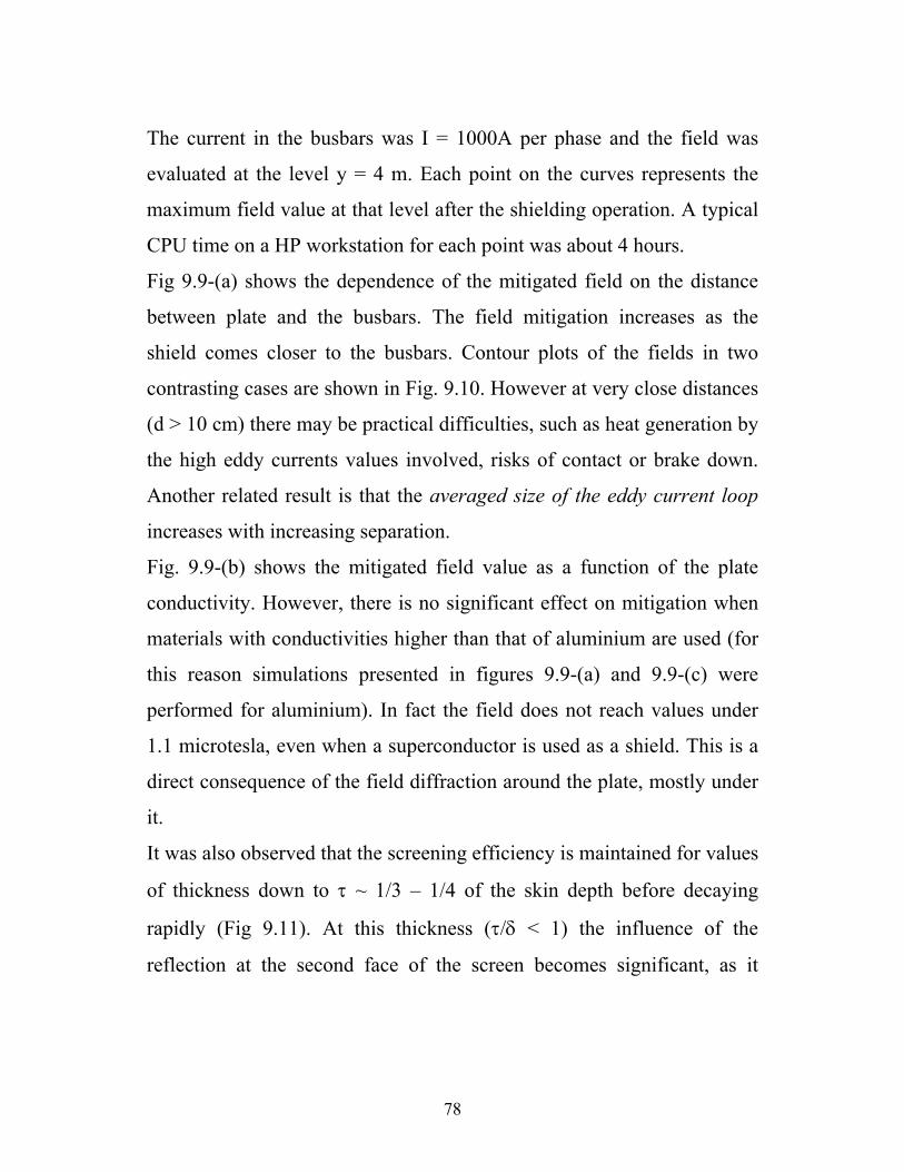
The current in the busbars was I = 1000A per phase and the field was
evaluated at the level y = 4 m. Each point on the curves represents the
maximum field value at that level after the shielding operation. A typical
CPU time on a HP workstation for each point was about 4 hours.
Fig 9.9-(a) shows the dependence of the mitigated field on the distance
between plate and the busbars. The field mitigation increases as the
shield comes closer to the busbars. Contour plots of the fields in two
contrasting cases are shown in Fig. 9.10. However at very close distances
(d > 10 cm) there may be practical difficulties, such as heat generation by
the high eddy currents values involved, risks of contact or brake down.
Another related result is that the averaged size of the eddy current loop
increases with increasing separation.
Fig. 9.9-(b) shows the mitigated field value as a function of the plate
conductivity. However, there is no significant effect on mitigation when
materials with conductivities higher than that of aluminium are used (for
this reason simulations presented in figures 9.9-(a) and 9.9-(c) were
performed for aluminium). In fact the field does not reach values under
1.1 microtesla, even when a superconductor is used as a shield. This is a
direct consequence of the field diffraction around the plate, mostly under
it.
It was also observed that the screening efficiency is maintained for values
of thickness down to τ ~ 1/3 – 1/4 of the skin depth before decaying
rapidly (Fig 9.11). At this thickness (τ/δ < 1) the influence of the
reflection at the second face of the screen becomes significant, as it
78

contributes to the attenuation of the incident field (appendix II), much as
reflection of light by dielectric materials with high εr .
0
2
4
6
8
10
12
14
0 0.2 0.4 0.6 0.8 1 1.2 1.4
Plate Th ickne ss(τ )/ Pe ne tration De pth(δ )
Scre
enin
g Ef
ficie
ncy
(S)
[dB
]
τ = δ = 12 mmτ = 3 mm
Fig. 9.10 Two examples of magnetic flux density reduction. In both cases the conductivity of the plate is σ = 3x10⁷ S m-1 and its thickness is 3 mm. In (a) the shield is at d = 50 cm from the bus bars, while in (b) it is at d = 3 cm.
(b)
d = 3 cm d = 50 cm
Magnetic field at y = 4 m (without shielding) ~ 4.55 microtesla
Magnetic field at y = 4 m ~ 0.51 microtesla
Magnetic field at y = 4 m ~ 2.5 microtesla
(a)
Fig. 9.11. Shielding efficiency of an aluminium plate at y = 4m as a function of τ/δ.
79

Diffraction of the field around the shield produces eddy currents on the
other side of the plate. This effect is more evident as the separation
between plate and busbars d increases, as can be observed in Fig. 9.12. In
Fig. 9.8 the shielding plate was not located symmetrically with respect to
the busbars system because the floor restricted the positioning of the
plate. This restriction, however, can be removed, for instance in the
design of the substation or switchboard, allowing symmetrical
positioning of the plate. Results of simulations for the symmetrical case
shows that this operation improves the field mitigation (Fig. 9.13).
Magnetic field( B) vs plate thickness (τ ) for different plate-busbars separation (d)
0
0.5
1
1.5
2
2.5
3
3.5
4
4.5
5
0 2 4 6 8 10 12 14 16
Plate thickness (mm)
B (m
icro
tesl
a)
d = 8 cm
d = 20 cm
d = 10 cm
d = 15 cm
Fig. 9. 12 Influence of the positioning of the shielding plate on the diffraction of the field around the plate, y = 4m.
80

B (at y = 4m) vs distance
0.79
1.36
1.82
2.19
2.46
2.69
0.42
0.84
1.34
1.75
2.11
2.4
-
0.50
1.00
1.50
2.00
2.50
3.00
- 0.10 0.20 0.30 0.40 0.50 0.60 0.70
Distance plate-busbars (meters)
B (m
icro
tesl
a)
Fig. 9.13 Magnetic field in function of the distance for two different geometries. Except for the positioning of the aluminium plate all the parameters are the same as in Fig. 9.9-(a). The lower curve represents the case when the shield is symmetric with respect to the busbars.
9.5 Ferromagnetic shielding The results in section 9.4 were obtained for the conductive shielding.
However, the same formulation can be applied to ferromagnetic
shielding. In fact, the new formulation should be a generalization of the
conductive case since most of ferromagnetic materials considered in
practical applications of shielding have a non-negligible conductivity.
Results expressed as shielding efficiency (SE) considering a
ferromagnetic plate are shown in Fig. 9.14. In all the simulations a linear
relation between B and H was assumed.
Fig. 9.14 shows that a conductive material gives a more efficient
screening than a ferromagnetic one [6]. This is in apparent contradiction
with the concept of skin effect, which gives for iron (σ = 1.07x10⁷ Sm-1,
and µr = 250) a skin depth δ = (π f µ0 µr σ)-1/2 ~ 0.14cm, almost an order
81

of magnitude less than for aluminium – Hence better efficiency would be
expected. The latter is correct right at the other side of the ferromagnetic
screen, where a strong reduction is observed (Fig. 9.15). However, at 4 m
over the system, the two properties of iron, conductivity and magnetic
permeability, are in antagonism, as the first tries to cancel the field, the
other tries to attract the field lines. In fact some of the field lines are
pulled into the region where we want to mitigate the field.
0
2
4
6
8
10
12
14
16
18
0 0.1 0.2 0.3 0.4 0.5 0.6Busbars-Screen Separation (d)
[metres]
Schi
eldi
ng E
ffici
ency
(SE)
[d
B] Iron
µr = 500 σ = 1.07 x 10⁷ Sm-1
Aluminium µr = 1 σ = 3.77 x 10⁷ Sm-1
Fig. 9.14 Screening efficiency as a function of the distance between busbars and screen.
82

(b)
Ferromagnetic shielding iron plate (σ = 1.03x10⁷ Sm−1 , µr = 500)
(a)
Conductive shielding aluminium plate (σ = 3.77x10⁷ Sm−1)
Fig. 9. 15. Contour lines of the magnetic field for two shielding configurations with the same geometry and current configuration. The only difference is that the two plates are made of different materials (a) aluminium, and (b) iron.
9.6 Recommendations The results from the various simulations provide some suggestions for
cost-effective mitigation of fields originated from busbar systems. The
following practical criteria can be given:
83
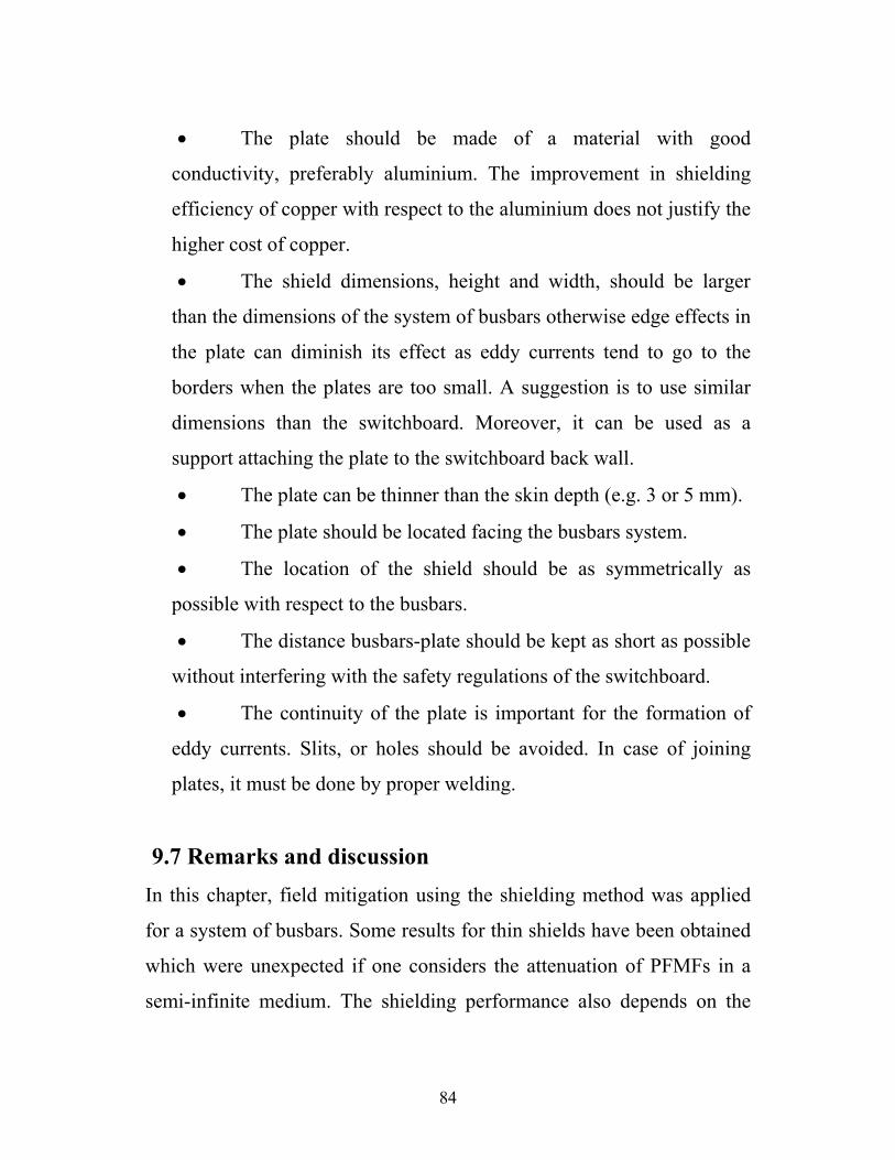
• The plate should be made of a material with good
conductivity, preferably aluminium. The improvement in shielding
efficiency of copper with respect to the aluminium does not justify the
higher cost of copper.
• The shield dimensions, height and width, should be larger
than the dimensions of the system of busbars otherwise edge effects in
the plate can diminish its effect as eddy currents tend to go to the
borders when the plates are too small. A suggestion is to use similar
dimensions than the switchboard. Moreover, it can be used as a
support attaching the plate to the switchboard back wall.
• The plate can be thinner than the skin depth (e.g. 3 or 5 mm).
• The plate should be located facing the busbars system.
• The location of the shield should be as symmetrically as
possible with respect to the busbars.
• The distance busbars-plate should be kept as short as possible
without interfering with the safety regulations of the switchboard.
• The continuity of the plate is important for the formation of
eddy currents. Slits, or holes should be avoided. In case of joining
plates, it must be done by proper welding.
9.7 Remarks and discussion In this chapter, field mitigation using the shielding method was applied
for a system of busbars. Some results for thin shields have been obtained
which were unexpected if one considers the attenuation of PFMFs in a
semi-infinite medium. The shielding performance also depends on the
84

geometrical configuration of the arrangement of the source and shield.
Moreover, due to the inherent characteristics of eddy currents, the
shielding method can involve some counter-intuitive properties. For
example, let us consider another configuration such as locating the
shielding plate horizontally over the busbars. This configuration may
look as an efficient shield because it seems to be “protecting” (as an
umbrella under the rain) the area to be mitigated. However evaluation of
the shielding efficiency shows that this arrangement hinders the flows of
eddy currents that cancel the busbar’s field in an efficient way in Fig16-
(a). Out of the three geometries in Fig. 9.16 the most effective
configuration is that in Fig. 9.16-(a).
SE (4m) = 6.27 SE (4m) =10.49 SE (4m) = 14.67
(a) (c) (b)
y = 4m y = 4m y = 4m
Figure 9.16 Different configurations of busbars and shielding plate evaluated for reduction of the magnetic field at y = 4 m. The material and currents are the same. The most effective configuration is (a).
85

A related effect is given in Fig. 9.17. Adding a bending to the upper part
of the shield (attempting to create an “umbrella effect”) is not very
effective, since the currents formed in the bending are considerably small
compared to the ones in the front part of the plate.
Fig. 9.17 Adding a bending to the upper part of a conductive shield. Eddy currents are much smaller in that part of this shield.
Double shielding also presents some interesting possibilities, Fig. 9.18
shows a comparison between the system Al-Fe-Source compared to the
permutation Fe-Al-Source. In both cases a coil of 20 cm diameter,
carrying a current of 100 A (50 Hz) was used. The plate was (2 metres
wide) x (1 metre high) x (3 + 3 mm) thick. The separation between plate
and coil was 10 cm. Another interesting result is:
In double shielding, the closeness of the conductive plane to the source provides a better field mitigation.
86

Fig 9.18 Mitigation by double shielding, comparison of the effect of permutation of aluminium and Iron. There is no actual separation between both plates.
No Shield - Source
Aluminium - Iron - Source
Iron - Aluminium - Source
87

88
Besides the double layer discussion, only the simplest solutions for the
shielding problem were presented here because they involve low costs.
However, further improvements of the method are possible. The use of
multi-layer techniques (Appendix III), or different shielding shapes
(Paper D) can provide more costly but also more efficient shielding.
References [1] Clayton R. Paul, Introduction to Electromagnetic Compatibility, Wiley series in Microwave and Optical Engineering, john Wiley & Sons, Inc. N.Y. 1992. [2] Welsby, V. G., The Theory and Design of Inductance Coils., Macdonald&Co. Publishers Ltd., London, 1960, p. 67.
[3] Schulz, R. B., “Shielding Theory and Practice”, IEEE Transactions on Electromagnetic Compatibility, Vol. 30, No 3, 1988, pp. 187-201. [4] Moser, R., “Low-Frequency Low Impedance Electromagnetic Shielding”, IEEE Transactions on Electromagnetic Compatibility, Vol. 30, No 3, 1988, pp. 202-210. [5] E. Salinas, L. Aspemyr, J. Daalder, Y. Hamnerius, and J. Luomi, Power Frequency Magnetic Fields from In-house Secondary Substations. CIRED’99, 15th Conference on Electricity Distribution, Technical Reports, session 2, pp. 161-164. University of Liège, Belgium, June 1999. [6] E. Salinas, “Conductive and Ferromagnetic Screening of 50 Hz Magnetic Fields from a Three –Phase System of Busbars”, Journal of Magnetic and Magnetic Materials, 2001, Vol. 226-0/2002, pp 1239-1241.

10 Active and passive compensation ––––––––––––––––––––––––––––––––––––––––
he principle of active compensation was introduced in chapter 4.
This principle uses the properties of naturally induced currents and
imitates them by a designed electrical device. Passive compensation is
also based on eddy currents but instead of plates (in the case of shielding)
the paths of these currents are wires. In chapter 9, various properties of
eddy currents have been described. Thus, it is possible to utilize these
properties for elaborating compensating schemes.
T
10.1 Active compensation of busbars Analysis of eddy currents in a conductive plate at different instants
provides a hint of how to compensate the field of busbars. Fig. 10.1
shows the instantaneous configuration of eddy currents on a plate
located in front of a system of busbars, which is 2m long, with 2cm x
2cm cross-sections, and carrying a current of 100A in each of the phases
(R, S and T). The geometrical shapes of the paths of the eddy currents
can be understood as the dynamics of two loops. This detail is more
evident in the second frame of Fig 10.1. An “imitation” of these loops
can be constructed with two coils carrying two different 1-phase
currents, namely S and T, achieving in this way a 2-phase equivalent of
a 3-phase system of busbars. These two loops are designed to generate a
field similar but opposite to the field of busbars.
89

e) ωt = 120°
d) ωt = 90°
f) ωt = 180°
a) ωt = 0° b) ωt = 20°
c) ωt = 40°
Fig. 10.1 Instantaneous configurations of the paths of eddy currents on the surface of a shielding aluminium plate for different angles ωt.
In order to obtain an equivalent current of 100A per loop and at the
same time be able to connect the coils directly to the main feeding
circuit the number of turns (N = 60), wire thickness and impedance was
calculated. Thus the feeding current in each of the compensating coils
was only 1.67A. The uppermost and lowermost sides of the
90

compensating coils then have opposite currents to the S and T branches
of the busbars. The middle part of the coil arrangement yields an
equivalent current with phase -S-T =-R, that will compensate the middle
branch of the busbars (Fig. 10.2).
1.67A
+120°
-120°
T
S
100 A
-120°
0°
+120°
R
T
S
Fig. 10.2 Busbars (3-phase) and compensating coils (1-phase each). The coils are placed in front of the busbars.
The shielding efficiency at y = 1.5 m from the busbars was measured
experimentally (Fig. 10.3) varying the parameter distance (d) busbars-
coils. It varies from SE = 8.6 dB to SE = 15.4 dB, when the distance d
between busbars and coil vary between d = 20 cm and 10 cm
respectively. The efficiency gets higher for smaller values of d.
However, influence on design rules and safety regulations (e.g. too high
values of the mutual impedance, and appearance of induced forces when
d < 10 cm) do not allow the placement of coils too close to the busbars.
91

Busbars
Compensating coils
Fig. 10.3 Experimental implementation of active compensation. Each coil is 2m long and 0.25 m wide.
Fig. 10.4 shows the result of a FEM simulation for active compensation
(presented in two contour plots shaded regions for initial conditions and
shaded regions for the compensated case). The attenuation factor
obtained was about 13 dB for the external values (B0 = 0.1 µT).
With coils
No coils 0.1 µT
Fig. 10.4 Busbars: field after active compensation (lines) contrasted with the field without shielding (contour regions).
92
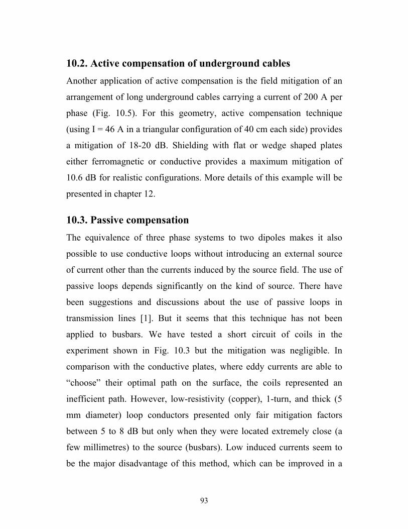
10.2. Active compensation of underground cables Another application of active compensation is the field mitigation of an
arrangement of long underground cables carrying a current of 200 A per
phase (Fig. 10.5). For this geometry, active compensation technique
(using I = 46 A in a triangular configuration of 40 cm each side) provides
a mitigation of 18-20 dB. Shielding with flat or wedge shaped plates
either ferromagnetic or conductive provides a maximum mitigation of
10.6 dB for realistic configurations. More details of this example will be
presented in chapter 12.
10.3. Passive compensation The equivalence of three phase systems to two dipoles makes it also
possible to use conductive loops without introducing an external source
of current other than the currents induced by the source field. The use of
passive loops depends significantly on the kind of source. There have
been suggestions and discussions about the use of passive loops in
transmission lines [1]. But it seems that this technique has not been
applied to busbars. We have tested a short circuit of coils in the
experiment shown in Fig. 10.3 but the mitigation was negligible. In
comparison with the conductive plates, where eddy currents are able to
“choose” their optimal path on the surface, the coils represented an
inefficient path. However, low-resistivity (copper), 1-turn, and thick (5
mm diameter) loop conductors presented only fair mitigation factors
between 5 to 8 dB but only when they were located extremely close (a
few millimetres) to the source (busbars). Low induced currents seem to
be the major disadvantage of this method, which can be improved in a
93
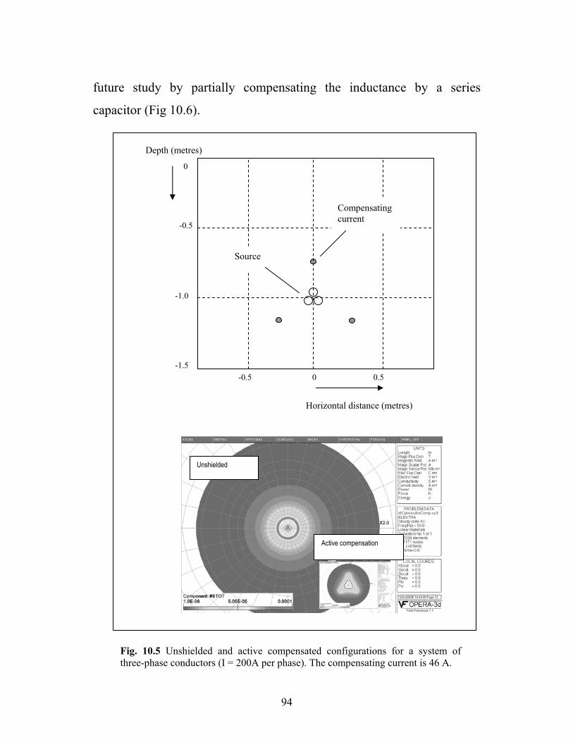
future study by partially compensating the inductance by a series
capacitor (Fig 10.6).
Source
Compensating current
Horizontal distance (metres)
Depth (metres)
-1.5
-1.0
0 -0.5 0.5
-0.5
0
Active compensation
Unshielded
Fig. 10.5 Unshielded and active compensated configurations for a system of three-phase conductors (I = 200A per phase). The compensating current is 46 A.
94

(a) (b)
B
A
Loops Source
d (c)
Compensating loop Capacitor
Fig 10.6 Passive compensation schemes.
References [1] U. Johnsson, A. Larsson and J-O. Sjödin, “Optimized Reduction of magnetic field near Swedish 400 kV lines by advanced control of shield wirecurrents. Test results and economical evaluation”, IEEE trans. Power Delivery, Vol. 9, April 1994, pp. 961-969. [2] H. Olsson, Petersson, A. Eriksson, “Reduction of Transmission Line Magnetic Field-Possibilities and Constraints”, CIGRE Report 36-101, 1990.
95

96

11 Mitigating the field of transformers
––––––––––––––––––––––––––––––––––––––––
here are various kinds of distribution transformers. The most
common type is the oil-insulated transformer; also dry transformers and
epoxy-insulated transformers are used.
T
In liquid/oil-immersed units a sealed tank construction, made of steel,
effectively contains the windings and active parts in an optimal
environment, as the liquid substance is both an insulating and a cooling
agent. Because of their design losses are minimised – in fact, these units
are very efficient and can operate in an overload condition up to 30% for
several hours. On the other hand, they are considered and handled as
flammable items and as such less suitable for domestic or public places.
Dry transformers neither contain any cooling liquid nor are they inside
sealed metal containers. Their coils have a varnish impregnation, are cast
in epoxy resin, or surrounded by other insulating materials, which are
capable of leading excessive heat away. These types of transformers are
often highly fire resistant. Their use is most advantageous in high-risk
places (e.g. oil refineries or nuclear plants), public buildings (e.g.
hospitals, airports), or dense residential areas.
The magnetic field from transformers is rather complex and has various
origins, such as the leakage field from the coils and ferromagnetic
laminations, or the connections at the low/high voltage parts. To model
the complete field emission from a transformer is rather a difficult task.
97

Attempts have been made to use numerical methods to deal with various
parts of transformers [1], [2]. Because of this complexity, the shielding
characteristics have to be obtained experimentally. Even though small-
scale experiments can help to decide upon some suitable shielding
features [3], they do not provide definitive answers since the magnitude
of a transformer’s magnetic field do not scale linearly with its size.
Therefore actual-size experiments have to be performed.
11.1 Comparison between a shielded and an unshielded transformer Two commercially available transformers were studied [4], one
unshielded (TU) (Fig. 11.1), and the other shielded (Fig. 11.2) with a 5
mm aluminium box cover (TS). Fig. 11.3 shows a comparison of the field
from these transformers and other substation components. Although the
transformers TU and TS have different manufacturers and different
designs (both of them are dry, but TS is varnished and TU is epoxy cast),
they have various similarities. Both are 800 kVA, three-phase, and were
connected to the same feeding transformer in similar configurations as to
provide a comparison. The comparison showed that the shielding cover
was the most relevant differentiating factor between the two
transformers. Design of both transformers involved secondary
connections situated at the bottom of the transformer and tests were made
with optimal cable connections (Fig. 11.2).
The shielding efficiency (SE) of the shield of TS relative to TU, showed
values that were about 15 dB in average in an area 4m x 4m above the
98

transformer, at h = 3 m over the floor of the substation. The field from
internal connections (on the transformer’s secondary side) of TS and the
stray field from coils and core were mitigated via eddy currents by the
aluminium box. In addition, it was demonstrated that the emission from
TS was about 50% lower compared with the averaged values of the field
from the switchboard, which was part of the experimental set ups.
Fig. 11.1 Epoxy insulated dry transformer, unshielded (TU).
Optimal cable connections
Fig. 11.2 Varnish coated dry transformer, shielded (TS).
99

1 3 5 7 9 11 13 15 17 19 21 23 25 27
S10
0 .20 .40 .60 .81
1 .21 .41 .61 .82
2 .22 .42 .62 .83
B (m
icro
tesl
a)
X
S w r.
2 .8 -32 .6 -2 .82 .4 -2 .62 .2 -2 .42 -2 .21 .8 -21 .6 -1 .81 .4 -1 .61 .2 -1 .41 -1 .20 .8 -10 .6 -0 .80 .4 -0 .60 .2 -0 .40 -0 .2
Cables
Shielded transformer (TS)
Unshielded transformer (TU)
Switchboard
itchb oard + M o ere T r . vs F rance TI=400A, z=3m
Switchboard + TS + TU I = 400A, h = 3m
Y
x (metres)
Fig. 11.3 The field from various components of a secondary substation. The shielded transformer gives a field emission that is significantly lower as compared with the unshielded one.
100

11.2 The largest contribution to the field of the transformers
In the former section, the secondary connections were located at the
lower side of the two transformers. In addition, these connections were
optimised by phase grouping. However, in functioning substations, which
were not designed for low field emission, this is not necessarily the case,
as is presented in the following example.
The substation (10/0.4 kV, 800 kVA) located at Haga (in central
Gothenburg) was studied. The contour plots of the magnetic field, at the
floor above the substation, are given in Fig. 11.4. The analysis of the
highest field values and its gradient along the vertical direction provided
a negative reply to the conjecture that these values may be originating
directly (i.e. coils or core) from the transformer T1. The field values at 1
metre above the floor means about 4 metres above the floor of the
substation, therefore much lower fields are expected from T1 than the
ones read in Fig. 11.4-(b). In fact, the source seems to be much closer to
the ceiling and decaying in a different way than a transformer’s field [4].
A simple internal inspection established that the large separation between
phases (R, S and T) was responsible for the high field values (Fig. 11.6-
a). Moreover, the low voltage connections followed a long path rather
close to the ceiling of the substation (Fig. 11.5 and 11.6-b). However the
cables along this path were well packed allowing for field self
cancellation. Large phase separation was not observed at the other
transformer (T2) since the connections were rather direct (Fig. 11.6-c)
and following a short distance path to the low-voltage switchboard.
101

To approach this problem, a modification in phase configuration is
suggested (Fig. 11.7). The cables should be kept packed all the way to
the very end at the secondary side of T1, where they can be reconnected
to the transformer individual phases. 3D-simulations for obtaining the
magnetic field of the total cable arrangement were performed. The
comparison between the two arrangements (Fig. 11.8) gave a good field
mitigation expressed in a mitigation efficiency of about 18 dB at the
locations of maximum values. Since the resulting values can still be
considered high, an improved solution is suggested (Fig. 11.9), which
consists of various stages: (i) upside down positioning of the transformer,
(ii) phase rearrangement, (iii) connections to the low voltage side at the
floor level or, if possible, by the cellar of the substation, and (iv) eventual
shielding of the transformer. Future implementation of these measures is
expected to mitigate the field to values at the sub-microtesla level.
References
[1] J. Turowski and A. Pelikant, IEE. Proc.- Electr. Power Appl., Vol. 144, No. 6, 1997, pp. 435-440.
[2] J. Shen, Z. Andrelic and B. Schaub, IEE Trans. on Magn. Vol. 34. No 5, 1998, pp. 2636-2639.
[3] T. Zhong. “Field mitigation from power transformers”, Master thesis (in preparation), Chalmers University of Technology, 2001.
[4] E. Salinas and L. Aspemyr, Experimental Study of 50 Hz Magnetic Fields from 10/0.4 kV Substation Components. Proceedings of the Fourth Latinamerican Congress on Electrical Generation, Transmission and Distribution, Vinha del Mar, Chile, November 2000.
102

103
Fig. 11.4 Contour plot of the magnetic field one floor above Haga substation.
B (microtesla)
(a)
1 2 3 4 5 6 7 8 9 10 11 12 13
S1
S2
S3
S4
S5
S6
20-2218-2016-1814-1612-1410-128-106-84-62-40-2
1 2 3 4 5 6 7 8 9 10 11 12 13
S1
S2
S3
S4
S5
S6
5.00-6.00
4.00-5.00
2.00-3.00
1.00-2.00
0.00-1.00
Haga Substation Magnetic field contour map at one floor above
Measurements at the floor level Taken on Nov. 21, 2001 (17:30-19:00)
B (microtesla)
(b) Haga Substation
Magnetic field contour map at one floor above Measurements at 1 metre over the floor level
Taken on Nov. 21, 2001 (17:30-19:00)
3.00-4.00

Fig 11. 5 Configuration of Haga substation. T1 has a split-phase/joint operation, while T2 is directly connected to the low voltage switchboard.
T1 T2
Swtich-board Split
phase
Joint phase
S T
R
(b)
(c)
(a)
Fig 11.6 Interior of Haga substation. The responsible for the high fields on the floor above the substation is the large separation between phases (a) in transformer T1. The cables from the secondary side of T1 follow an upper trajectory (b) to the low voltage switchboard. The connection of transformer T2 is more suitable for low field emission.
104

To the low-voltage switchboard
To the low-voltage switchboard
R S T
R S T
R S
T
Fig. 11.7 phase split and phase reconfiguration at the connections of transformer T1.
105

After phase arrangement
Before phase arrangement
1.25 µT
1.75 µT 2.25 µT
2.75 µT 0.75 µT
0.25 µT
12 µT9 µT
6 µT
3 µT 23 µT
18 µT15 µT
Fig. 11.8 Contour plot at the floor level before and after phase rearrangements.
106

Fig. 11.9 The optimal solution for minimizing the field of Haga substation is: (i) upside down positioning of the transformer, (ii) phase rearrangement, (iii) connections to the low voltage side by the cellar of the substation and (iv) eventual shielding of the transformer.
Upside down position
Cellar of substation
Original configuration
Shield
107

108

12 Examples of field mitigation ––––––––––––––––––––––––––––––––––––––––
S
ome of the techniques developed in this report can be applied to
actual cases where the measured values of the magnetic field are
considered as problematic. One example was already described in section
11. 2, and a few more are presented in this chapter. These examples also
helped to develop mitigation techniques, since the most adequate method
was often not known in advance. Sometimes the cases yielded
unexpected results, as in the case of stray currents (sections 12.2-12.3).
A course of action frequently used was: (i) measurement of the field, (ii)
analysis of the data and modelling, which provided hints for the choice of
mitigation techniques, (iii) implementation of the mitigation proposals,
and iv) measurement of the field after mitigation. However, sometimes
the issue required the application of mitigation schemes before the
installations became operative, i.e. already at the design level, to ensure
low field emission. In that case, modelling was more relevant.
12.1 Measurement of PFMFs In order to measure magnetic fields, various devices have been designed.
They are known under various names: gaussmeter, magnetic field meter,
magnetic field dosimeter, magnetic field logger, and for the particular
frequency of interest in this work: power frequency magnetic flux density
meter, or simply magnetometer. Most of them are based on the same
principle that was used for conductive shielding and passive
109

compensation i.e. the induction principle. The magnetic field generates a
voltage signal in a coil with a large number of turns. This signal has to be
amplified and electronically processed before it is displayed. The
necessary components of these instruments are: detection coils,
integration circuits, time-averaging devices, filters and amplifiers (Fig.
12.1). Measured quantities are given in rms (root mean square) values.
B
Coil
Normal to Coil
Time averaging
Amplifier Filter Display (µT)
Integration
Fig. 12.1 Structure of a typical magnetometer.
There are two kinds of field meters: single-axis magnetometers and
three-axis magnetometers. The first one measures the magnitude of the
magnetic field along the axis perpendicular to the detection coil. The
second contains three perpendicular coils. To measure single-phase fields
the first instrument is rather useful since it can even determine the
direction of the field. In a three-phase system, the magnetic field is
elliptically polarized, therefore quite difficult to determine its rms-value
by a single-coil instrument. In that case, the second type of magnetometer
is needed. The magnitude of the magnetic field is in this case determined
by:
110

Brms = Bx ,rms( )2
+ By ,rms( )2
+ Bz ,rms( )2
(12.1)
The instrument most frequently used in this project is a magnetic field
logger1. This instrument belongs to the second type and can register the
rms-value of the magnitude (but not the direction) of the magnetic field,
which can be seen directly on the display. The values are displayed in
microtesla. The range of frequencies (bandwidth) this instrument can
detect is between 30 Hz and 2000 Hz.
12.2 The fields at the Gothenburg City Library Here a study is presented of magnetic fields originating from a secondary
substation located in the cellar of the Gothenburg City Library
(Göteborgs stadsbibliotek). This public library (Fig. 12.2) is located in
the centre of Gothenburg and is surrounded by other public and urban
buildings. About 190 persons work in this building and around 3,000
visit each day.
The electricity supply to the library and nearby public buildings consists
of a secondary 10/0.4 kV substation (two 800 kVA, three phase
transformers). The configuration of the components is shown in Fig.
12.3-(a).
1 EnviroMentor ML-1
111

Fig. 12.2 Two views of the City Library, its location (up) at Götaplatsen and its interior (right). The secondary substation is located in the cellar of the building.
Extensive measurements were made [1] of the 50 Hz magnetic field at
the floor above the substation. Figure 12.4-(a) shows the distribution of
the magnetic field. Field values of around 1-4 microtesla were registered
in areas right above the location of the substation. Values up to 6
microtesla were measured in areas under which there were no substation
parts. Moreover, the field contour curves corresponding to these values
followed a diagonal across the room. Thus the presence of stray currents
(see next section) was suspected. Using analytical calculations [1] it was
possible to determine the equivalent value (10-15 amperes) and the
112

location of these currents (0.5-0.75 meters under the floor of the reading
room).
Various modifications were proposed, not only by installing new
substation components, but also altering their geometrical disposition in
the room of the substation, as shown in figure 12.3-(b). The main
modifications were:
• Replacement of the unshielded transformers with new low emission
transformers with an aluminium cover.
• A shielding of aluminium (5mm-thick plate) welded to the back of the
low voltage switchboard. Additionally a 5mm welded aluminium
shield lined the ceiling and the back of the low-voltage switchboards
of the substation.
• The cable connections between components were positioned under the
floor. Prior to the renovation some cables were positioned over the
floor, some even close to the ceiling.
• A modern high voltage switchboard with low magnetic field emission
characteristics replaced the previous one.
After the modification of the substation a series of measurements were
again performed in the same area. The contour plot of these values is
shown in figure 12.4-(b). Most of the values registered on the region
right above the substation were well under 1 microtesla and had an
average value of 0.5 microtesla. It can be noted that there is a peak value
(in a very small region) of 1.1 microtesla. Additional measurements of
113

this value along the vertical distance gave a rapid decay according to
1/(distance)3, thus it was suspected that the origin of this maximum was
not the substation components but a local source. The source was later
found to be the motor of a cooling fan installed at the ceiling of the
substation.
In the same figure it can be observed that the values of the field due to
stray currents, though still high, have an appreciable different distribution
than before the renovation. This is due to the fact that stray currents have
a broad variation in time.
The last part consisted in reducing the field due to stray currents. There
are two methods to achieve this; one is to install a five conductors
system; the other is to install magnetic field reducers. The first solution is
very costly and the second option was adopted. The stray current is a
problem that is not the domain of the utilities but of the customer.
Therefore the field reduction procedures were decided and carried out by
the owners of the building. Ferromagnetic cores were installed, which
surround the cable forming a booster transformer, thus forcing the net
current in the cable to be reduced. The result after installing the reducers
is shown in figure 12.4-(c). The average field on the area above the
substation has also diminished.
If one takes into account that a former alternative was to relocate the
substation, which represented a difficult and costly option, the decision to
modify the substation produced significant cost reductions to the utility.
114
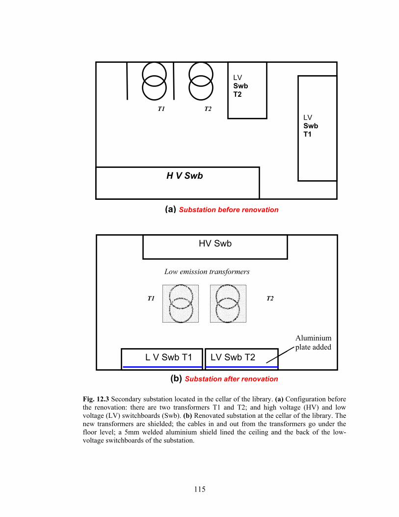
Low emission transformers
LV Swb T2
T2T1
HV Swb
L V Swb T1
Aluminium plate added
(a) Substation before renovation
LV Swb T2
T2 T1
LV Swb T1
H V Swb
(b) Substation after renovation
Fig. 12.3 Secondary substation located in the cellar of the library. (a) Configuration before the renovation: there are two transformers T1 and T2; and high voltage (HV) and low voltage (LV) switchboards (Swb). (b) Renovated substation at the cellar of the library. The new transformers are shielded; the cables in and out from the transformers go under the floor level; a 5mm welded aluminium shield lined the ceiling and the back of the low-voltage switchboards of the substation.
115

116
(a)
(b)
(c)
Fig. 12. 4 The magnetic field one floor above the library and its reduction at different stages.

Cable rearrangement Shielded transformers
Compact HV switchboard Shielded busbars
Magnetic field reducers
Fig 12. 5 Measures taken to mitigate the field from the substation at the Gothenburgs City Library.
117

12. 3 Stray currents The most common type of cable configurations installed in houses and
connected to electrical appliances contains two parallel conductors
carrying opposite currents. These conductors are close to each other and
the total magnetic field, in principle, nearly cancels (a similar statement
is valid for a larger number of cables).
Stray currents are one of the most common sources of magnetic fields in
Sweden (and other countries that have similar cable connections
systems); these are currents that escape from an intended electric circuit
and return. Such currents may run along pipes, and spread to
neighbouring houses, instead of staying along the neutral conductor,
which is intended to carry the current back to the feeding system.
This problem is common in a four-conductor system. Fig. 12.6 shows the
principle of stray currents; a simplified diagram of a four-conductor
system shows the division of a load current (I) into the return (In) and a
stray current (Iw) running along metallic water pipes.
An interesting characteristic of stray currents is that they are not possible
to mitigate using conductive shielding, since induced currents need a
returning path. Neither can they be passive or actively compensated for
similar reasons.
A solution to it is to add an extra cable (five-conductor system), which
will give the current a direct return path to the ground of the feeding
system, without dividing or spreading (Fig. 12.7). Another solution is to
use magnetic field reducers (see section 12.2), which are connected along
the line carrying stray currents. The former solution is economically
118
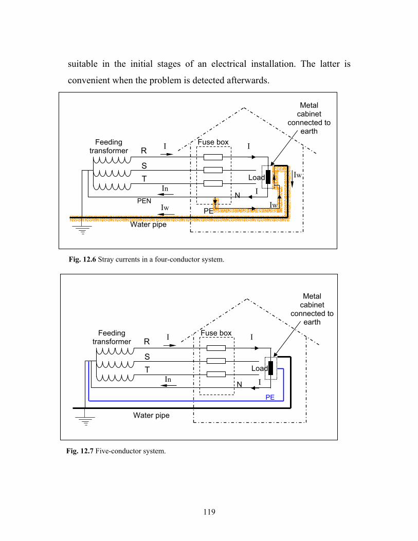
suitable in the initial stages of an electrical installation. The latter is
convenient when the problem is detected afterwards.
PE
Water pipe
I Fuse box
Load
Metal cabinet
connected to earth
In
I
T S
R Feeding
transformer
I N
I
Iw
Water pipe
I
PEN
Fuse box
Load
Metal cabinet
connected to earth
PE Iw
In
I
T S
R Feeding
transformer
Fig. 12.6 Stray currents in a four-conductor system.
N Iw
Fig. 12.7 Five-conductor system.
119

12. 4 Magnetic fields at the renovated Electrical Power Engineering building
Another case in which it was possible to test some of the tools developed
for mitigation of PFMFs was the renovation of the Electrical Power
Engineering (Institutionen för Elteknik) building at Chalmers. The study
and reduction of the fields were executed as the same time as the
renovation of the secondary substation took place; thus the project was
bounded in time, therefore results were to be obtained in a form readily
to be applied. For details see reference [2]
Figure 12.9 shows the distribution of the main components of the
substation (10/0.4 kV, 2 x 800 kVA). The magnetic field was measured
on the floor above the substation (a conference and IT room was going to
be located on that floor), particularly at the level of 3 and 4 meters above
the busbar system. A realistic configuration and maximum values of
currents were assumed; usually the currents involved are much smaller.
The values of the field registered before reduction operations are shown
in figure 12.9-(a). In order to study the magnetic field emitted by the
substation, analytical calculations and numerical simulations (using the
2D-FEM program ACE) were performed. It was found that a plate of
aluminium a few millimetres thick was enough to bring down magnetic
field values to levels recommended by the Swedish building board [3].
An aluminium plate (3 mm thick, 13 m wide and 2 m high) was welded
to the back of the switchboard. The measured values after the reduction
of the magnetic field are shown in figure 12.9-(b). At the present time the
values at the studied areas are below the recommended levels, even under
high load conditions.
120

(a)
Busbars 4m below
0.4
0.1
0.2 (b) 0.07
0.15
1.04
0.7
0.33
0.19
0.18
0.49
0.45
0.08 0.28
0.21 0.48 0.23
0.77
Fig. 12.8 Representation (not in scale) of some of the major components of the substation at Elteknik. The busbars are inside a switchboard made of steel. Only one of the transformers is connected at the time. The Aluminium shield is 3mm thick, 13m wide and 2m high.
4 mAluminium shield
T2 T1
Level of interest
13 m
Busbars
1 m
Fig. 12. 9 Magnetic field values before (a) and after (b) the field reduction operation. The values were taken at the plane located 4m above the busbar configuration.
121

12.5 Shielding of underground cables Shielding of PFMFs from power lines by using metal plates is difficult be-
cause of the lack of support for metal settings. In the case of underground ca-
bles, the shielding option exists, as the soil provides a natural support for ar-
rangements of metal plates.
Here, the case of a three-phase 130 kV system of underground cables is ana-
lysed (Fig 12.10). The system consists of 200 m long cables located at 1 m
under the ground. They carry a nominal current of 200A/phase, having each
cable a cross section with outer diameter of 83 mm, and inner conductor di-
ameter of 26.4 mm.
The cables are placed in a triangular configuration. It can be assumed that the
ground has µ = 1, σ = 0 and does not have any relevance in the field computa-
tions. It does, however, define the area of interest 10m x 2m, and sets eco-
nomical restrictions to the choice of mitigation method, as digging and instal-
lation costs are involved.
S
R
T
Area of interest
1m
2m10m
Fig. 12.10 Three-phase underground cables below an area of interest. e.g. a children’s play-ground.
122

Four different configurations were modelled in two dimensions using Opera
and compared with the initial field (no-shield) case. In all cases the length of
the shields (or compensating cables) were as long as the cable length.
y
x
-S -T
-R
1m
(d)
(a) (b)
(c)
5 cm
20 cm20 cm
40 cm
Fig. 12. 11 Different shielding configurations for the magnetic field of underground cables (a) 1 m plate, (b) - (c) continuous wedge 90 cm wide and bent 90°. Active compensation was also consid-ered (d).
Case (a): A flat metal plate, 1 metre wide and 5 mm thick, is located d = 20
cm above the cables.
123

Case (b) - (c): A wedge-shaped metal plate, 90 cm wide, 5 mm thick and 90°
bent, is located at (b) d = 20 cm, and (c) d = 5 cm respectively, above the ca-
bles.
Case (d): Active compensation by a three-phase system of cables, forming an
external triangle of 40 cm per side and carrying a current I = 46 A per phase.
(Fig. 12.11-c) The phases on the external triangle are opposite (-R, -S, -T) to
the ones in the interior triangle.
In the cases of shielding with metal plates, the following materials were used:
Table 12.1 Materials
Material Conductivity, Sm-1 Relative permeability (µr) Aluminium 3.77 x 10⁷ 1 Iron 1.03 x 10⁷ 250, 500, 1000, 1500, 2000
Fig 12.12 shows an example of a FEM simulation in Opera. The complexity of
the field around a shielding configuration is evident.
Fig. 12.12. Field around a shielding configuration, wedge-shaped iron plate, µr = 250, d = 5 cm.
124

The simulations for the cases of shielding and compensation give, for different
vertical distances, the following magnetic field values:
Table 12.2 Case a: Flat shield (d = 20 cm)
B (microtesla) y = 1m y = 2m y = 3m
No shield (B0 ) 4.06 µT 1.02 µT 0.455 µT Al 2.43 µT 0.69 µT 0.312 µT Fe 250 2.36 µT 0.65 µT 0.296 µT Fe 500 2.35 µT 0.65 µT 0.294 µT Fe 1000 2.29 µT 0.66 µT 0.287 µT Fe 1500 2.26 µT 0.63 µT 0.284 µT Fe 2000 2.24 µT 0.62 µT 0.282 µT
Table 12.3 Case b: Wedge shield (d = 20 cm) B (microtesla) y = 1m y = 2m y = 3m
No shield (B0) 4.06 µT 1.02 µT 0.455 µT Al 1.85 µT 0.49 µT 0.210 µT Fe 250 2.03 µT 0.52 µT 0.233 µT Fe 500 2.05 µT 0.52 µT 0.235 µT Fe 1000 2.01 µT 0.51 µT 0.229 µT Fe 1500 1.98 µT 0.50 µT 0.225 µT Wedge-Fe 2000 1.95 µT 0.49 µT 0.222 µT
Table 12.4 Case c: Wedge shield (d = 5 cm)
B (microtesla) y =1m y = 2m y = 3m No shield (B0) 4.06 µT 1.02 µT 0.455 µT Al 1.19 µT 0.30 µT 0.141 µT Fe 250 1.94 µT 0.56 µT 0.335 µT Fe 2000 2.23 µT 0.63 µT 0.285 µT Table 12.5 Case d: Active compensation, Extras: Double-layer shielding B (microtesla) y = 1m y = 2m y = 3m No shield (B0) 4.06 µT 1.02 µT 0.455 µT Active compensation 0.78µT 0.13µT 0.05µT Wedge Al (d = 10 cm) 1.2 µT 0.36 µT 0.170 µT Wedge (d=10cm)-Double-Fe-Al 1.8 µT 0.47 µT 0.216 µT
125

Evaluation of the shielding efficiency yields the following results (for the dif-
ferent methods according to the best mitigation factors obtained in each case)
Table 12.6 Average shielding efficiency
METHOD
Flat shield (d=20cm)
Wedge shield (d =20cm)
Wedge shield (d = 5cm)
Active Compensation
Average Shielding Efficiency (SE) 4.6 dB
6.3 dB 10.5 dB 17.5 dB
Consequently, the mitigation method that gives maximum field attenuation -for
this particular case of underground cables- is active compensation. Fig. 12.13
shows the global mitigation effect of the compensating cables.
Maximum filed attenuation not necessarily means a cost-effective method.
Cost-efficiency should additionally take into consideration:
i) Cost of energy supply on the compensation cables.
ii) Maintenance cost.
Remark: It is interesting to notice that, as in section 6.1, the mitigation factors
for active compensation evaluated from table 12.5 give an increase of the
shielding efficiency (SE) with the distance:
SE (1m) = 14.3 db, SE (2m) = 17.9 dB, SE (3m) = 19. 5 dB.
Is this a general characteristic of efficient mitigation techniques? Certainly it
deserves more study. This behaviour is not necessarily present in other -less
efficient- methods (e.g. shielding with Al and Fe [mu=2000] in case a, table
12.2).
Another remark is that, at the design stage, i.e. before starting cable installa-
tion, the possibility of applying phase-split may be considered (e.g. section 6,
126

Fig 6.4). This method is cost effective only when is performed at the initial
stages.
1 µT
10 µT
10 µT
1 µT
Fig. 12.13 Mitigation by active compensation.
127

12.6 Mitigation from electrical service rooms
Distribution panels and other electrical installations in small rooms are com-
plementary to substations. It is not unusual to find them in different floors of
buildings. Sometimes they can emit high values of PFMFs since they contain
small busbars and several conductors.
Here, the shielding of an electrical room with dimensions of a rectangular
box, 3.5 m x 2.0 m per side, was modelled in two dimensions using opera. A
semi-open shield was used (Fig. 12.14).
(0,0)3500 mm
1000 mmX
Y
3 mm 2 mm
2000 mm
Fig. 12.14 Shielding of a small electric service room using a semi-open shield.
128

Test source: The sources were: two sets 3-phase busbars; cross section: 4 mm x 2 mm; separation between busbars: 10 cm. Current I = 100 A (rms). Materials tested:
• Aluminium: conductivity = 3.77 x 10^7 S/m, relative permeability = 1 • Transformer steel (96% Fe + 4% Si): conductivity = 0.18 x 10^7 S/m,
average linear relative permeability = 1000.
Results:
Fig. 12.15 and 12.16 show the FEM meshing and the field from the sources in
the absence of a shield.
Fig. 12.17 shows the field (in the range: 0.05 < B < 2 microtesla) using a
shield of iron, 5 mm thick.
Fig. 12.18 shows the field (in the range: 0.05 < B < 2 microtesla) using a
shield of aluminium, 5 mm thick.
Fig. 12.19 shows the comparison of the field in an interesting region, between
y =3m and y =5 m.
Conclusions
A semi-closed shield made of 5 mm aluminium yielded the best field attenua-
tion (over 20 dB). However a cover of 3 mm is suggested as a possible cost-
effective solution (Fig 12.19).
Cost-effective solutions choosing closed, or semi-closed shields covering the
walls and ceiling of a room are feasible only for small rooms, for larger ones
it is advisable to consider shielding of the sources.
129

Fig. 12.15 Fields originating in an electrical service room. Range: 0.05 µT < B < 2µT.
Fig. 12.16 Shielding with a semi-close shield made of 5 mm iron. Range: 0.05 µT < B < 2µT.
130

Fig. 12.17 Shielding with 5 mm aluminium semi-closed shield. Range: 0.05 µT < B < 2µT.
No shield
Al 5 mm Al 3 mm
Fe 5 mm Fe 3 mm
Fig. 12.18 Comparison between different shields for a vertical distance: 3m < y < 5m.
131

12.7 Summary of Mitigation methods Table 12.7 shows several methods that were applied or discussed in this work.
The study of these strategies by application to actual cases may bring im-
provements to our knowledge on mitigation of PFMFs.
Table 12.7
Source Field mitigation strategy
Design method
Busbars, long (> 5m) • Shielding • Active compensation
• 2D-FEM • Analytical
Busbars, short (< 5m) • Shielding • Active compensation • Compact design
• 3D-FEM • Experimental
3-phase transformers • Shielding • Placing connections by
the lower side
• Experimental • 3D-FEM
Cables, connections
• Phase rearrangement • Relocation of cable
paths.
• Analytical
High voltage transmis-sion lines (aerial)
• Phase-split • Active compensation • Passive compensation
• Analytical • Experimental
Underground cables • Shielding, • Active compensation • Phase-split
• 2D-FEM • Analytical
Small Electrical service rooms
• Semi-closed shields • Shielding of components
• 2D/3D-FEM
132

References [1] E. Salinas, L. Aspemyr, J. Daalder, Y. Hamnerius, and J. Luomi, “Power Frequency Magnetic Fields from In-house Secondary Substations”, CI-RED’99, 15th Conference on Electricity Distribution, Technical Reports, ses-sion 2, pp. 161-164. University of Liège, Belgium, June 1999. [2] E. Salinas and L. Aspemyr, Measurements and Reduction of 50 Hz Mag-netic Fields from the New Substation at the Department of Electric Power Engineering. Technical Report No. 14R, ISSN: 1401-6176, Department of Electric Power engineering, Chalmers University of Technology, Gothen-burg, 1999. [3] The Swedish: National Board of Occupational Safety and Health, Na-tional Board of Housing, Building and Planning, National Electrical Safety Board, National Board of Health and Welfare, Radiation Protection Institute, Low-Frequency Electrical and Magnetic Fields: The Precautionary Principle for National Authorities, Solna, Sweden, 1996.
133

134
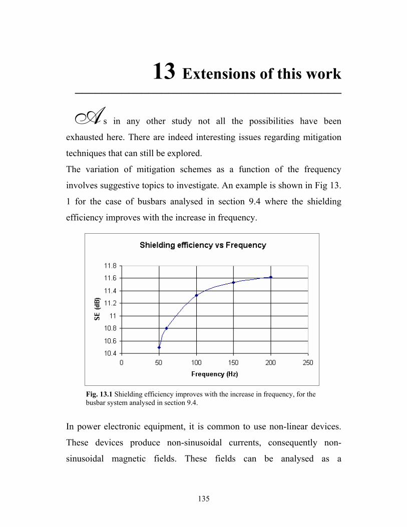
13 Extensions of this work ––––––––––––––––––––––––––––––––––––––––
s in any other study not all the possibilities have been
exhausted here. There are indeed interesting issues regarding mitigation
techniques that can still be explored.
A
The variation of mitigation schemes as a function of the frequency
involves suggestive topics to investigate. An example is shown in Fig 13.
1 for the case of busbars analysed in section 9.4 where the shielding
efficiency improves with the increase in frequency.
Fig. 13.1 Shielding efficiency improves with the increase in frequency, for the busbar system analysed in section 9.4.
In power electronic equipment, it is common to use non-linear devices.
These devices produce non-sinusoidal currents, consequently non-
sinusoidal magnetic fields. These fields can be analysed as a
135
136
superposition of the fundamental frequency (50 Hz) and their harmonics.
Usually, but not always, the most relevant harmonics in a power system
are the 3rd (150 Hz), the 5th (250 Hz) and the 7th (350 Hz). A distinctive
problem caused by harmonic distortion are the high currents that may
appear in the neutral conductor. As in the case of stray currents (section
12.3), a current in the neutral conductor is difficult to mitigate.
Consequently, a systematic study of the effects of harmonics on the
mitigation schemes is needed.
More experimentation is also needed. On the one hand, precise testing of
some of the mitigation techniques can verify some of the results of this
study. Small-scale experimentation can clearly save costs and time. Thus
transformations of the parameters involved in mitigation schemes –in
order to obtain scale-invariant results– need to be developed. On the
other hand, more case studies are also needed in order to apply and
improve the strategies developed in this study.
Active and passive compensation need further studies and improvements.
Even though this study aimed at the search for simple and cost-effective
solutions for mitigating PFMFs, combination of techniques such as active
compensation and shielding may represent improved solutions for
mitigation.
Some of the modeling methods used here can certainly be extrapolated to
deal with problems in some other areas of engineering or science in
which modeling of electromagnetic fields represents a valuable tool.

14 Conclusions ––––––––––––––––––––––––––––––––––––––––
his thesis has investigated various schemes to mitigate power-
frequency magnetic fields. It has focused on secondary substations,
which represent the end points of the electrical distribution network and
are located in the surroundings of residential buildings and highly
populated areas. For this reason the magnetic fields emitted by these
installations should be considered as important as the –much debated–
fields from power lines. Electromagnetic compatibility and the increasing
concern for health related issues were the motivations for the initiation of
this project.
T
The transformer is the heart of a substation (and cables and busbars are
its arteries and veins!). Therefore one may think that the magnetic field
of the transformer represents a major contribution to the total field of a
substation. This study, however, has shown that busbars and the ill self-
cancelling fields of connections at the low voltage part of the substation
are frequently the main contributors. Moreover, the field in the
surroundings of a substation can have other origins such as stray currents.
This type of source produces a field that decays slowly with the distance.
In fact, this problem is rather common in Sweden due to its 4-conductor
system.
This thesis showed that it is possible to achieve cost-effective mitigation
of PFMFs down to sub-microtesla levels. Cables can be optimally
137

grouped and positioned in order to give maximum field cancellation.
Stray fields from coils and the iron core of a dry transformer can be
reduced by an aluminium box. The field of busbars can be shielded by a
thin aluminium plate, symmetrically located and at a short distance.
These techniques are simple and not very costly to implement in
comparison to the shielding of extensive areas. The methods developed
were applied to study cases as strategies rather than a precise medium for
testing each of the techniques. In fact, some of these cases were worked
out at the same time that mitigation techniques were being developed.
Some of the techniques developed in this study can readily be applied to
operative substations, while others can only be applied during the design
stages. In addition, some of the strategies developed in this work are also
valid for other parts of the electric network.
As the XXI century takes form, more technology is inevitable,
consequently an increase of PFMFs is expected. At the same time
development of sustainable societies is in growing demand. If we
consider the electromagnetic field as part of such an environment,
hopefully the methods developed in this study may contribute to the
mitigation of unwanted magnetic field emissions in those societies.
138

Appendices
139

140

Appendix I: The field from a differential segment of current
––––––––––––––––––––––––––––––––––––––––
o solve the apparent contradiction presented in chapter 2, one can
assume the following argument, which is a “thought experiment”: let’s
imagine an experimental set up (Fig. 1) in which the piece of wire
representing the small element of current is covered by a tubular
electrical insulator and immersed in a large container with a mercury bath
at very low temperature to enhance its conductivity. Say, at 3 °K, since at
4 °K the resistance of mercury drops dramatically. The edges of the
current element are not insulated thus the current is free to spread, which
it does in all directions, hence it is possible to add end to end myriads of
these insulated current elements as to form closed circuits filling the lines
shown in Fig. 1. Once this is done the conducting fluid is drained away
and would not contribute to any of the calculations. This spreading is
symmetric on each edge, thus at a distance r the magnetic field B will be
T
Mercury
3 °K
Fig. 1 Experimental set up to solve the contradiction of charge conservation.
141

distributed on a circle, as is shown in Fig. 2. In order to calculate B the
flow of current though the spherical cap of radius rc is evaluated and then
obtained by the application of the Ampere circuital law.
r
rc
i
B
θ-dθ θ
Fig. 2 Evaluation of the magnetic field B from a current element.
The current outflow through the spherical cap is given by
ic = current density x area of the cap
( ) ( )θθππ
cos12
cos124
22 −=−×=
irr
iic
Similarly, the current inflow through the cap is
( )[ ]θθ dii c −−=′ cos12
Thus the total flow is the subtraction of inflow to outflow
( )[ ] θθθθθ didiii cc sin2
coscos2
=−−=′−
Applying the Ampere law to the circuit at the border of the cap
′−=•∫ cc iid 0µlB
we obtain
142

θθµπ diBrc sin2
2 0=
From Fig. 2, rc = r sinθ, and r dθ = dl sinθ, consequently
θπµ sin4 2
0
ridlB = (1)
In vector form this equation reconstructs the formula Eq. 2.1 (chapter 2).
It is important to observe that the frequency of the current has not been
specified. Therefore this formula is valid for 50 Hz (AC) which is the
interest of this work, but even for continuous current (DC).
However for AC currents is possible another approach to the solution of
the physical contradiction, namely to consider that the element of current
consist of a charge attached to a harmonic oscillator, e.g. a spring (Fig 3).
B
θ
er
r
Q
dl
Fig. 3 An oscillating charge as model for the element of current.
The frequency of oscillation being 50 Hz, the current is i(t) = dQ /dt = I
cos ωt =Re [I e jωt]. The direction of the oscillation is assumed to be
along z. To determine the magnetic field of the system one can use the
retarded vector potential [1].
z
rj
redlI e
=− β
πµ
40 A
143

where β = ω/c. In spherical coordinates ez = er cos θ – eθ sin θ, thus the
magnetic field is obtained from the expression B = (1/µ0) curl A, giving
( )φ
β
ββθβ
πerje
rjrjIdl −
+−= 2
2 11sin4
B
When ω = 2πf = 100π, the region is in the near zone, (extremely low
frequency) hence βr = 2πr/λ << 1. Therefore the magnitude of field in
this approximation becomes
θπµ sin4 2
0
rIdlB = (2)
Which again in vector notation represents Eq. 1, or Eq. 2.1 in chapter 2.
Once the physical contradiction has been solved, Eq. 1 can be used to
evaluate the field from specific sources.
144

Appendix II : Penetration depth for thin screens
–––––––––––––––––––––––––––––––––––––
For a magnetic field with two components Bx and By we assume
propagation along the x-direction through a thin layer with conductivity
σ and thickness h and infinite in y-z plane. Applying Maxwell’s
equations at power frequencies to this model gives
EB σ0µ=×∇ (1)
BE ωj−=×∇ (2)
From these two equations
BB σ0ωµj−=×∇×∇ (3)
But B2∇−⋅∇∇≡×∇× BB∇ , and 0=⋅∇ B , therefore
BB σ02 ωµj=∇ (4)
With y-dependence proportional to , the x-dependence must be
where
jkyexe κ±
σ022 ωµκ jk =− (5)
Then we have the following formulation
jkykxceB += jkyxx ebeaeB )( κκ += − jkykxkx ereeB )( −+=
-h 0
Shield
Vacuum Vacuum
B = (Bx, By)
145

Applying continuity of Bx and By (which because of 0=⋅∇ B , is the
same than continuity for Bx and dBx/dx) and Boundary conditions at x =
0 and x = -h, we obtain that
fec
kh
= (6)
where
( )[ ] hk
khekekk
f hh κκκκκκ
κκκ sinh
2cosh)(
41 22
22 ++=−−+= − (7)
is the complex screening factor.
From Eq. 5
202 2σ
δωµκ jj =≅ (8)
then
δωµκ jj +
=+
=1σ
21
0 (9)
The penetration depth is
σωµδ
0
2= (10)
and in interesting cases k>>κ . Under this condition, an approximation
of f that holds for h << δ is
2
2
12
1δ
κk
hjhk
f +=+≅ (11)
Note that since kδ << 1 if k>>κ , f can be >>1 even if h < δ.
Therefore a screen that is thinner than the skin depth can give significant
shielding. Also note that this effect is more significant for fields with
long wavelength (small k) transverse to the screen.
146

Appendix III : Shielding of coils –––––––––––––––––––––––––––––––––––––
A series of 3D simulations were performed with the coil described in
section 9.3 in front of an open shield. Single, conductive and
ferromagnetic; double, triple, and active shielding were simulated.
Parameters such as distance to the shield and thickness were varied.
Experimental verification was also carried out (e.g. Fig. 1 and Fig. 2).
Some relevant information is given by the external shape (size) of the
figures. It suggests a global comparison between all the cases (Fig. 3).
0.01
0.1
10.1 1 10
Vertical distance (m)
B (m
icro
tesl
a)
Coil + Shield (Aluminium plate, 3mm)
0.001
0.01
0.1
1
10
0.1 1 10
Vertical distance (m)
B (m
icro
tesl
a)
Fig. 2 Simulation vs. experiments, of the field of a coil, when a 3 mm aluminium plate is placed, at 15 cm from the coil. At distances larger than 1.5 metres, the magnetic background of the laboratory produces interference.
Fig. 1 Simulation vs. experiments, of the field from a coil, when no shield is placed.
Background field (noise)
Experiments
Simulations
10Coil, no shield
147
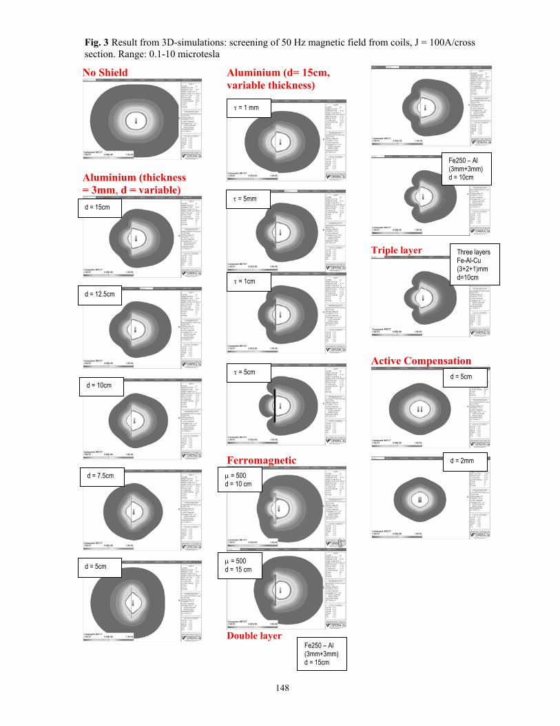
Fig. 3 Result from 3D-simulations: screening of 50 Hz magnetic field from coils, J = 100A/cross section. Range: 0.1-10 microtesla
No Shield
Aluminium (thickness = 3mm, d = variable)
Aluminium (d= 15cm, variable thickness)
Ferromagnetic
Double layer
τ = 1 mm
τ = 5mm d = 15cm
Triple layer
τ = 1cm
d = 12.5cm
Active Compen
τ = 5cm
d = 10cm
µ = 500 d = 10 cm
d = 7.5cm
µ = 500 d = 15 cm d = 5cm
148
Fe250 – Al (3mm+3mm)d = 10cm
Three layers Fe-Al-Cu (3+2+1)mm d=10cm
sation
d = 5cm
d = 2mm
Fe250 – Al (3mm+3mm)d = 15cm

List of Articles Paper A E. Salinas, L. Aspemyr, J. Daalder, Y. Hamnerius, and J. Luomi, Power Frequency Mag-netic Fields from In-house Secondary Substations. Published at CIRED’99, 15th Conference on Electricity Distribution, Technical Reports, session 2, pp. 161-164. University of Liège, Belgium, June 1999. Paper B E. Salinas and A. Bondeson, Shielding of Power Frequency Magnetic Fields from a Three-Phase System of Busbars. Published at IEEE-ANDESCON’99, International Conference of the IEEE Andean Re-gion, Proceedings paper No. I031, Universidad Simon Bolívar, Caracas, Venezuela, Sep-tember 1999. Paper C E. Salinas and L. Aspemyr, Experimental Study of 50 Hz Magnetic Fields from 10/0.4 kV Substation Components. Published in the Proceedings of the Fourth Latinamerican Congress on Electrical Gener-tion, Transmission and Distribution, Vinha del Mar, Chile, November 2000. Paper D E. Salinas and L. Aspemyr, Measurements and Reduction of 50 Hz Magnetic Fields from the New Substation at the Department of Electric Power Engineering. Technical Report No. 14R, ISSN: 1401-6176, Department of Electric Power engineering, Chalmers University of Technology, Gothenburg, Sweden, August 1999. Paper E E. Salinas, A. Bondeson, J. Daalder and Y. Hamnerius Towards a Global Strategy to Mitigate Power Frequency Magnetic Fields from Secon-dary Substations. Published in proceedings of CIRED’2001, 16th Conference on Electricity Distribution, IEE Conference Publication No 482, Technical Theme 2, Paper 2.5, Amsterdam, 2001. Paper F E. Salinas, Studies of Magnetic Fields at the Transmission and Distribution Stages Accepted for publication (August, 2001) in Journal of the IES on M&E Special Issues. Paper G E. Salinas, Conductive and Ferromagnetic Screening of 50 Hz Magnetic Fields from a Three-Phase System of Busbars. To be published in Journal of Magnetism and Magnetic Materials, 2001, Vol. 226-230 (2001), pp 1239-1241.