MARINE ECOLOGY PROGRESS SERIESMar Ecol Prog Ser

Vol. 213: 229–240, 2001 Published April 4

INTRODUCTION

Pelagic environments are characterized by verticalchanges in light, temperature, turbulence, transport,food and predators. These conditions vary non-uni-formly in space and time. As a result, zooplankton facea highly variable environment in which to feed, mate,avoid predators and recruit to satisfactory habitats.The vertical distribution patterns and movements ofzooplankton reflect evolved strategies for dealing withthese conditions. In turn, the vertical distributionsaffect other processes, such as feeding by planktivo-rous fishes. Despite the importance of vertical positionto vital rate functions (feeding, respiration, reproduc-

tion) and trophic interactions, only a few of the possibleenvironmental stimuli and corresponding zooplanktonresponses are known well enough to be predictive. Forexample, in the past, different studies provided con-flicting evidence about the prevailing depth distribu-tion patterns of species and diel patterns of verticalmigrations (DVM: Hays et al. 1997). Recent findingshave shown substantial plasticity in DVM patternswhen certain predators are present (Neill 1990, 1992,Ohman 1990, Bollens & Stearns 1992, Frost & Bollens1992). This accounts for some of the prior conflictingdata and suggests that the risk of predation weighsheavily among the factors influencing this behavior.Turbulent mixing also affects zooplankton behavior(Costello et al. 1990, Saiz & Alcaraz 1992, Saiz 1994)and has been associated with changes in zooplankton

© Inter-Research 2001

*E-mail: lincze@bigelow.org

Changes in copepod distributions associated withincreased turbulence from wind stress

L. S. Incze1,*, D. Hebert2, N. Wolff1, N. Oakey3, D. Dye1

1Bigelow Laboratory for Ocean Sciences, West Boothbay Harbor, Maine 04575, USA2Graduate School of Oceanography, University of Rhode Island, Kingston, Rhode Island 02882, USA

3Bedford Institute of Oceanography, Dartmouth, Nova Scotia B2Y 4A2, Canada

ABSTRACT: Vertical profiles of turbulent kinetic energy dissipation rate (ε), current velocity, tem-perature, salinity, chlorophyll fluorescence, and copepods were sampled for 4 d at an anchor stationon the southern flank of Georges Bank when the water column was stratified in early June 1995.Copepodite stages of Temora spp., Oithona spp., Pseudocalanus spp., and Calanus finmarchicus, andall of their naupliar stages except for Temora spp., were found deeper in the water column when tur-bulent dissipation rates in the surface mixed layer increased in response to increasing wind stress.Taxa that initially occurred at the bottom of the surface mixed layer at 10 to 15 m depth (ε ≤ 10–8 Wkg–1) before the wind event were located in the pycnocline at 20 to 25 m depth when dissipation ratesat 10 m increased up to 10–6 W kg–1. Dissipation rates in the pycnocline were similar to those experi-enced at shallower depths before the wind event. After passage of the wind event and with relaxationof dissipation rates in the surface layer, all stages returned to prior depths above the pycnocline.Temora spp. nauplii did not change depth during this period. Our results indicate that turbulencefrom a moderate wind event can influence the vertical distribution of copepods in the surface mixedlayer. Changes in the vertical distribution of copepods can impact trophic interactions, and move-ments related to turbulence would affect the application of turbulence theory to encounter and feed-ing rates.

KEY WORDS: Turbulence · Zooplankton · Vertical distribution · Vertical migration · Chlorophyllmaximum · Stratification · Mixing

Resale or republication not permitted without written consent of the publisher

Mar Ecol Prog Ser 213: 229–240, 2001

vertical distributions (Buckley & Lough 1987, Mackaset al. 1993, Haury et al. 1990,1992, Incze et al. 1990,Checkley et al. 1992, Lagadeuc et al. 1997). Moreover,small-scale turbulence may directly affect feedingrates of zooplankton (Yamazaki et al. 1991, Kiørboe &Saiz 1995, Saiz & Kiørboe 1995, Osborn 1996) andlarval fish (Dower et al. 1997, MacKenzie & Kiørboe1995, 2000) through changes in shear velocities andmodifications of feeding and searching behavior (Saiz1994, Mackenzie & Kiørboe 1995). While the intensityof turbulence in the upper ocean is strongly correlatedwith the wind stress (Oakey & Elliott 1982, Mackenzie& Leggett 1991), the vertical structure of small-scaleturbulence may be quite complicated (Denman & Gar-gett 1988, Gargett 1989). This places limits on the use-fulness of proxy variables for estimating turbulence atdiscrete depths and inferring behavioral and other ratefunctions for the resident plankton (Mullin et al. 1985,Yamazaki & Osborn 1988, Simpson et al. 1996, Gargett1997).

Since turbulence is ubiquitous and highly variable,a better understanding of zooplankton responses tochanging turbulence, as well as any preferences forcertain ranges, is needed in order to predict and inter-pret distributions and their biological consequences.At the same time, better information is needed con-cerning the structure of turbulence within the surfacemixed layer and the pycnocline, where many of thebiological interactions take place. In this paper weexamine the relationship between measured, in situturbulence and the vertical position of several abun-dant copepod taxa on the stratified southern flank ofGeorges Bank, off the northeastern coast of the USA.

Georges Bank, historically noted for its high fisheriesproduction (Brown 1987), is approximately 300 kmlong × 175 km wide. The crest of the bank (<50 mdeep) remains mixed throughout the year by the com-bined energy of winds and strong tidal currents (Horneet al. 1996), while at depths >60 m the water columnbecomes stratified during warm months of the year.Stratification begins in May and lasts until fall, whenit is eroded by seasonal surface cooling and increasedwind mixing (Flagg 1987). Residual circulation isclockwise around the bank and is well developedduring the stratified period (Butman et al. 1987, Lime-burner & Beardsley 1996). The physics and biology ofthe bank are being investigated through the currentUS and Canadian GLOBEC programs (Wiebe et al.2001), of which this study is a part.

MATERIALS AND METHODS

Data were collected on the southern flank of GeorgesBank from 11 to 15 June 1995. The vessel was an-

chored at 40.86° N, 67.54° W throughout the samplingperiod in a nominal depth of 75 m of water (Fig. 1).

Microstructure measurements of temperature, salin-ity and velocity were made with a tethered free-fallprofiler (EPSONDE: Oakey 1988) that was deployedfrom the stern of the vessel and descended at 0.5 to1 m s–1 until it hit the bottom. The sensor packagewas recessed 5 cm behind a circular, 30 cm-diameter,stainless steel lander. The tether was a kevlar multi-conductor payed out loosely ahead of the falling pro-filer and used for data transmission and instrumentrecovery. Velocity fluctuations were measured by 2shear probes sampling at 256 Hz. From 10 to 20 pro-files were collected in rapid succession over a 0.5 to1.7 h time period and were grouped into ‘sampleensembles’. Ensembles were initiated, on average,every 2.4 h except for a period of adverse winds andcurrent directions. Turbulent kinetic energy dissipa-tion rates (ε, in units of W kg–1) were derived from thevelocity fluctuation profiles (Oakey & Elliott 1982). Thedata were analyzed in 2 s segments blocked so that thelast segment ended on the last data point where theinstrument was still falling. Power spectra for the 2shear profiles were computed, frequency-responsecorrections for the sensors and electronic transfer wereapplied, and variance due to spikes and noise wasremoved (Oakey 1982). All of the profiles in an en-semble were averaged together in 2 dbar depth binsusing the maximum likelihood estimator for a log-normal distribution (Baker & Gibson 1987). Data fromthe upper 8 m were not used because they were conta-minated by turbulence created by the current flowingpast the anchored research vessel.

230

Fig. 1. Portion of the southern flank of Georges Bank showinglocation (+) where RV ‘Seward Johnson’ anchored for micro-structure and zooplankton profiling on 11 to 15 June 1995.Open square measures 20 × 20 km and encompasses thewater area advected past the anchor station during the courseof measurements (cf. Fig. 6); solid circle shows location of

NOAA Buoy 44011

Incze et al.: Copepod distributions and wind-induced turbulence

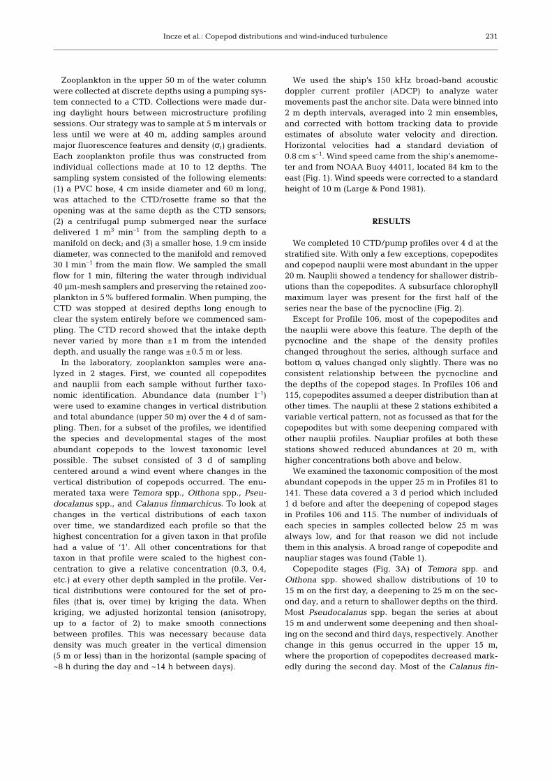
Zooplankton in the upper 50 m of the water columnwere collected at discrete depths using a pumping sys-tem connected to a CTD. Collections were made dur-ing daylight hours between microstructure profilingsessions. Our strategy was to sample at 5 m intervals orless until we were at 40 m, adding samples aroundmajor fluorescence features and density (σt) gradients.Each zooplankton profile thus was constructed fromindividual collections made at 10 to 12 depths. Thesampling system consisted of the following elements:(1) a PVC hose, 4 cm inside diameter and 60 m long,was attached to the CTD/rosette frame so that theopening was at the same depth as the CTD sensors;(2) a centrifugal pump submerged near the surfacedelivered 1 m3 min–1 from the sampling depth to amanifold on deck; and (3) a smaller hose, 1.9 cm insidediameter, was connected to the manifold and removed30 l min–1 from the main flow. We sampled the smallflow for 1 min, filtering the water through individual40 µm-mesh samplers and preserving the retained zoo-plankton in 5% buffered formalin. When pumping, theCTD was stopped at desired depths long enough toclear the system entirely before we commenced sam-pling. The CTD record showed that the intake depthnever varied by more than ±1 m from the intendeddepth, and usually the range was ±0.5 m or less.

In the laboratory, zooplankton samples were ana-lyzed in 2 stages. First, we counted all copepoditesand nauplii from each sample without further taxo-nomic identification. Abundance data (number l–1)were used to examine changes in vertical distributionand total abundance (upper 50 m) over the 4 d of sam-pling. Then, for a subset of the profiles, we identifiedthe species and developmental stages of the mostabundant copepods to the lowest taxonomic levelpossible. The subset consisted of 3 d of samplingcentered around a wind event where changes in thevertical distribution of copepods occurred. The enu-merated taxa were Temora spp., Oithona spp., Pseu-docalanus spp., and Calanus finmarchicus. To look atchanges in the vertical distributions of each taxonover time, we standardized each profile so that thehighest concentration for a given taxon in that profilehad a value of ‘1’. All other concentrations for thattaxon in that profile were scaled to the highest con-centration to give a relative concentration (0.3, 0.4,etc.) at every other depth sampled in the profile. Ver-tical distributions were contoured for the set of pro-files (that is, over time) by kriging the data. Whenkriging, we adjusted horizontal tension (anisotropy,up to a factor of 2) to make smooth connectionsbetween profiles. This was necessary because datadensity was much greater in the vertical dimension(5 m or less) than in the horizontal (sample spacing of~8 h during the day and ~14 h between days).

We used the ship’s 150 kHz broad-band acousticdoppler current profiler (ADCP) to analyze watermovements past the anchor site. Data were binned into2 m depth intervals, averaged into 2 min ensembles,and corrected with bottom tracking data to provideestimates of absolute water velocity and direction.Horizontal velocities had a standard deviation of0.8 cm s–1. Wind speed came from the ship’s anemome-ter and from NOAA Buoy 44011, located 84 km to theeast (Fig. 1). Wind speeds were corrected to a standardheight of 10 m (Large & Pond 1981).

RESULTS

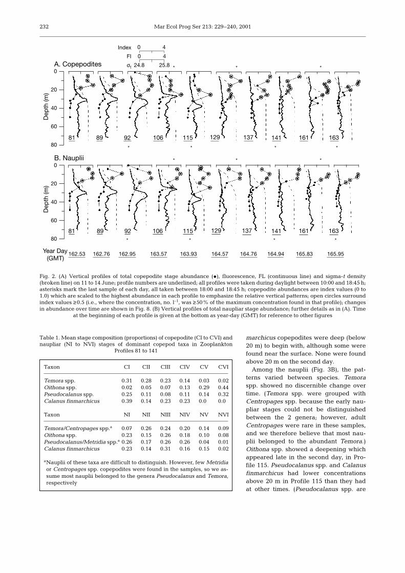
We completed 10 CTD/pump profiles over 4 d at thestratified site. With only a few exceptions, copepoditesand copepod nauplii were most abundant in the upper20 m. Nauplii showed a tendency for shallower distrib-utions than the copepodites. A subsurface chlorophyllmaximum layer was present for the first half of theseries near the base of the pycnocline (Fig. 2).

Except for Profile 106, most of the copepodites andthe nauplii were above this feature. The depth of thepycnocline and the shape of the density profileschanged throughout the series, although surface andbottom σt values changed only slightly. There was noconsistent relationship between the pycnocline andthe depths of the copepod stages. In Profiles 106 and115, copepodites assumed a deeper distribution than atother times. The nauplii at these 2 stations exhibited avariable vertical pattern, not as focussed as that for thecopepodites but with some deepening compared withother nauplii profiles. Naupliar profiles at both thesestations showed reduced abundances at 20 m, withhigher concentrations both above and below.

We examined the taxonomic composition of the mostabundant copepods in the upper 25 m in Profiles 81 to141. These data covered a 3 d period which included1 d before and after the deepening of copepod stagesin Profiles 106 and 115. The number of individuals ofeach species in samples collected below 25 m wasalways low, and for that reason we did not includethem in this analysis. A broad range of copepodite andnaupliar stages was found (Table 1).

Copepodite stages (Fig. 3A) of Temora spp. andOithona spp. showed shallow distributions of 10 to15 m on the first day, a deepening to 25 m on the sec-ond day, and a return to shallower depths on the third.Most Pseudocalanus spp. began the series at about15 m and underwent some deepening and then shoal-ing on the second and third days, respectively. Anotherchange in this genus occurred in the upper 15 m,where the proportion of copepodites decreased mark-edly during the second day. Most of the Calanus fin-

231

Mar Ecol Prog Ser 213: 229–240, 2001

marchicus copepodites were deep (below20 m) to begin with, although some werefound near the surface. None were foundabove 20 m on the second day.

Among the nauplii (Fig. 3B), the pat-terns varied between species. Temoraspp. showed no discernible change overtime. (Temora spp. were grouped withCentropages spp. because the early nau-pliar stages could not be distinguishedbetween the 2 genera; however, adultCentropages were rare in these samples,and we therefore believe that most nau-plii belonged to the abundant Temora.)Oithona spp. showed a deepening whichappeared late in the second day, in Pro-file 115. Pseudocalanus spp. and Calanusfinmarchicus had lower concentrationsabove 20 m in Profile 115 than they hadat other times. (Pseudocalanus spp. are

232

0

20

40

60

80

0

20

40

60

80

81 89 92 106 115 129 137 141 161 163

81 89 92 106 115 129 137 141 161 163

A. Copepodites

B. Nauplii

0 4Index

FI

σt

162.53 162.76 162.95 163.57 163.93 164.57 164.76 164.94 165.83 165.95

* * * *

Year Day(GMT)

* * **

Dep

th (m

)

* * *

Dep

th (m

)

* * *

0 4

24.8 25.8

Fig. 2. (A) Vertical profiles of total copepodite stage abundance (•), fluorescence, FL (continuous line) and sigma-t density(broken line) on 11 to 14 June; profile numbers are underlined; all profiles were taken during daylight between 10:00 and 18:45 h;asterisks mark the last sample of each day, all taken between 18:00 and 18:45 h; copepodite abundances are index values (0 to1.0) which are scaled to the highest abundance in each profile to emphasize the relative vertical patterns; open circles surroundindex values ≥0.5 (i.e., where the concentration, no. l–1, was ≥50% of the maximum concentration found in that profile); changesin abundance over time are shown in Fig. 8. (B) Vertical profiles of total naupliar stage abundance; further details as in (A). Time

at the beginning of each profile is given at the bottom as year-day (GMT) for reference to other figures

Table 1. Mean stage composition (proportions) of copepodite (CI to CVI) andnaupliar (NI to NVI) stages of dominant copepod taxa in Zooplankton

Profiles 81 to 141

Taxon CI CII CIII CIV CV CVI

Temora spp. 0.31 0.28 0.23 0.14 0.03 0.02Oithona spp. 0.02 0.05 0.07 0.13 0.29 0.44Pseudocalanus spp. 0.25 0.11 0.08 0.11 0.14 0.32Calanus finmarchicus 0.39 0.14 0.23 0.23 0.00 0.00

Taxon NI NII NIII NIV NV NVI

Temora/Centropages spp.a 0.07 0.26 0.24 0.20 0.14 0.09Oithona spp. 0.23 0.15 0.26 0.18 0.10 0.08Pseudocalanus/Metridia spp.a 0.26 0.17 0.26 0.26 0.04 0.01Calanus finmarchicus 0.23 0.14 0.31 0.16 0.15 0.02

aNauplii of these taxa are difficult to distinguish. However, few Metridiaor Centropages spp. copepodites were found in the samples, so we as-sume most nauplii belonged to the genera Pseudocalanus and Temora,respectively

Incze et al.: Copepod distributions and wind-induced turbulence

grouped with Metridia spp. because the naupliarstages are difficult to distinguish, but adult femaleMetridia spp. were rare on the southern flank.) Table 2summarizes the abundances of taxa used in Fig. 3; wesimplified the table by using the names Temora andPseudocalanus spp. without the other possible genera.

The ship’s meteorological data acquisition systemwas not working from Year Day 164.5 to 165.5, a periodof light wind following the principal wind event. Weused wind data from NOAA Buoy 44011 to fill in dur-ing this period. Wind speed data from the ship werehighly correlated with the buoy record when both sys-tems were operating during this study (n = 84 hourlycomparisons, r2 = 0.75, p << 0.001). Winds were 5 m s–1

or less for the first day of sampling (Profiles 81 to 92 inFig. 2). They increased to 10 m s–1 before Profile 106,and were steady through Profile 115 (data from theship’s record through this time period). By the follow-ing day (Profiles 129 and 137), winds were again lightand remained <8 m s–1 for the last 2 d of sampling(Fig. 4).

We completed 41 EPSONDE profiling ensembles in alittle over 4 d. Fig. 4 shows dissipation rates (ε) and sur-

face wind stress during the 3 d period when we did thefull taxonomic analysis. Epsilon values in the upper 10to 20 m of the water column were ≤10–8 W kg–1 before

233

B. Nauplii

0 .0

0.2

0.4

0.6

0.8

1.0

Temora Temora/Centropages

Oithona Oithona

Pseudocalanus Pseudocalanus

Calanus Calanus

A. Copepodites

163 163.5 164 164.5 163 163.5 164 164.5

Profile

Dep

th (m

)

81 92 106 115 129 141Profile

81 92 106 115 129 141

–5

–10

–15

–20

–25

–5

–10

–15

–20

–25

–5

–10

–15

–20

–25

–5

–10

–15

–20

–25

Dep

th (m

)

–5

–10

–15

–20

–25

–5

–10

–15

–20

–25

–5

–10

–15

–20

–25

–5

–10

–15

–20

–25

Year Day (GMT) Year Day (GMT)

Fig. 3. Vertical distributions of (A) copepodites and (B) nauplii of abundant copepod taxa in the surface mixed layer during 3 d(11 to 13 June), with a wind event on the second day. Shaded contours show index values (0.2 gradations) during daylight hours,

as in Fig. 2

Table 2. Maximum concentrations and integrated abun-dances (5 to 25 m) of copepod taxa in the pump profiles shownin Fig. 3. Data are means and (standard deviations) of all day-time profiles over 3 d. Integrated abundance was calculatedfor each profile by trapezoidal summation of concentrations

at each depth

Stages Max. profile Integrated abundanceconcentration from 5 to 25 m

(no. l–1) (no. m–2) × 1000

CopepoditeTemora spp. 17.9 (5.2)0 9.6 (3.4)Oithona spp. 34.8 (14.3) 23.3 (7.8)0Pseudocalanus spp. 11.4 (4.1)0 5.8 (1.5)Calanus finmarchicus 21.0 (13.9) 7.8 (3.5)

NaupliarTemora spp. 30.0 (9.9)0 9.7 (8.7)Oithona spp. 71.6 (22.4) 39.2 (13.0)Pseudocalanus spp. 92.3 (19.9) 59.3 (13.4)Calanus finmarchicus 27.5 (12.2) 12.7 (6.3)0

Mar Ecol Prog Ser 213: 229–240, 2001

Profiles 106 and 115. During Profiles 106 and 115, dis-sipation rates at 10 to 20 m ranged up to 10–6 W kg–1.After this, lower dissipation rates (ε ≤ 10–8 W kg–1) re-turned to the upper 10 to 20 m, although they wereinterspersed with some higher values. We used CTDdata from the EPSONDE to plot changes in densitystructure over time (Fig. 5). The pycnocline wasnearest the surface on the first day of sampling anddeepened on the second day. The deepening (ca YearDay 163.25 to 163.75) coincided with the onset andstrengthening of winds shown in Fig. 4. Temperatureswere around 8.5 to 10.5°C in the upper mixed layer,7 to 8°C in the pycnocline, and 6 to 6.5°C in the bottomlayer.

The current record at 15 m depth taken from theship’s ADCP shows that on- and off-bank excursions ofthe semi-diurnal tide were approximately 8 km at the

anchor site, and that the along-isobath residual velo-city averaged 3.8 km d–1 to the southwest. While allsampling took place at the anchor site, it is possible toinvert the ADCP record to back-calculate the approxi-mate initial geographical positions of the parcels sam-pled at 15 m depth (Fig. 6A). This calculation showsthat the samples came from within an area of about10 × 20 km. The largest along-isobath distance be-tween average daily positions of the zooplanktonpump samples was the ~5 km that separated Day 1from Day 2. The spatial distribution of the subsurfacechlorophyll maximum in the study area at the begin-ning of our profiling session is indicated in similar fash-ion by a back-calculation of the maximum fluores-cence values from all CTD casts (Fig. 6B). Analysis ofADCP data showed that horizontal shear over thedepth range from 15 m to the chlorophyll maximumwas small.

The distinct subsurface chlorophyll maximum layerthat was present when we began sampling disap-peared after Cast 115 (see profiles in Fig. 2). Was this atemporal phenomenon or a spatial one? Fig. 6B showsthat there was a strong horizontal spatial gradient inthe chlorophyll when we began our work. The highfluorescence region along the southern margin of thesampled area moved to the anchor site only during theon-bank portion of the tidal cycle. Pump profilesoccurred at various parts of the tidal cycle, samplingrelatively high chlorophyll concentrations throughCast 106, and thereafter missing them (Fig. 7). Theintegrated abundance of copepodites in each pumpprofile shows a slight decline after Cast 115 that per-sisted (Fig. 8). The shift after cast 115 coincided withsamples occurring outside the region of high chloro-phyll fluorescence (Fig. 6). Most of the decline in cope-podite abundance was due to a decline in Oithona spp.A small shift in naupliar abundance also occurred.

During April and May 1995, winds ≥10 m s–1 wererecorded 14% of the time at Buoy 44011. Most of theseoccurred as isolated events, similar to the event wesampled during this cruise.

DISCUSSION

It is often difficult to distinguish changes due to ver-tical processes from those resulting from horizontalvariability and advection. Since we sampled at a fixedsite, the ADCP record was essential for reconstructingthe flow field and helping to discriminate between thetemporal and spatial characteristics of our data. In thisstudy, the principal variables were the vertical distrib-ution and abundance of copepods, profiles of σt, fluo-rescence and turbulent kinetic energy dissipation rate,and wind. In this discussion we focus on processes in

234

163 163.5 164 164.5-10

0

10

20

-10

-20

-30

-40

-50

-60

-70

-9 -8.5 -8 -7.5 -7 -6.5 -6 -5.5 -5

Year Day (GMT)

Dep

th (m

)P

asca

l (x1

00)

Log10 Dissipation Rate (W kg–1)

Fig. 4. Hourly average wind stress (upper graph; positive Y isNorth) and average turbulent energy dissipation rate, ε (lowergraph), on 11 to 13 June. The white line at 26 m on lowergraph shows the lowest depth used in the detailed taxonomicanalyses shown in Fig. 3. The frequency of EPSONDE (Oakey

1988) profiling is shown in the bottom axis of Fig. 5

Incze et al.: Copepod distributions and wind-induced turbulence

the surface mixed layer and the pyc-nocline. The pattern of increasingand decreasing dissipation ratesbelow the pycnocline was generatedby tidal shear along the bottom,which we do not address further. Forconvenience, we use the word ‘tur-bulence’ instead of the term ‘dissipa-tion rate’ which was actually calcu-lated. We use the latter only whensupplying values to describe differ-ent levels of turbulence.

Our data show that most copepodstages on the stratified southernflank of Georges Bank in early Juneinhabited shallower depths, ~10 to15 m, when the surface was quies-cent (ε ~10–8 to 10–9 W kg–1) thanwhen it was turbulent. When dis-sipation rates at 10 m increasedup to 10–6.5 W kg–1, most of thecopepodites and many of the naupliiwere found at around 20 to 25 m.There, dissipation rates were similarto the values in which the copepodshad been residing previously. Fewcopepods were located below thislevel although the zone of low turbu-lence in our particular example ex-tended deeper (cf. Figs. 2 & 4). The

235

162.5 163 163.5 164 164.5 165 165.5 166

-35

-30

-25

-20

-15

-10

-5

Year Day (GMT)

Zooplankton Profiles

24.9

25.0

25.1

25.2

25.3

25.4

25.5

25.6

σt

Dep

th (m

)

EPSONDE Profiles

81 89 92 106 115 129 137 141 161 163

-5 0 5 10 15-5

0

5

10

15

4

3

2

1

B.A.

-5 0 5 10 15

East-West (km)

-5

0

5

10

15

Nor

th-S

outh

(km

)

Nor

th-S

outh

(km

)

Pump Stations

Day 1

Day 2

Day 3

Day 4

81

8992

106

115

129

137

141

161

163

East-West (km)

Fig. 5. Density (σt) structure in the upper 35 m, obtained from EPSONDE casts(614 profiles, shown on bottom axis). Year Day (GMT) and pump profile numbers

are given for reference to other figures

Fig. 6. (A) Theoretical trajectory (continuous line) of a water parcel at 15 m depth on 11 to 14 June, back-calculated from theanchor station (#81) using records from the ship-mounted 150 kHz broad-band Acoustic Doppler Current Profiler (ADCP); alldisplacements are shown relative to the first zooplankton profile at the origin (0, 0), making this a re-creation of synoptic posi-tions at the beginning of the observation period; numbers next to the symbols refer to zooplankton profiles; symbols distinguishbetween sampling days; axes are 20 km long and correspond to the square area in Fig. 1. (B) Maximum water-column fluores-cence values (shaded values, in volts) from all CTD casts beginning with Cast 81; the back-calculated positions of the casts (•)were derived from the ADCP record as above; the anchor station can be identified at the origin; the areal distribution of fluores-cence is a synoptic recreation and can be translated directly to (A); the vertical distribution of fluorescence at selected stations

can be seen in the profiles in Fig. 2

Mar Ecol Prog Ser 213: 229–240, 2001

change from shallow to deeper depths involved achange from the bottom of the surface mixed layer tonear the bottom of the pycnocline. Were the changes invertical distribution due to increased turbulence atthe surface, or were they due to other factors such asadvection, changes in pycnocline depth, or changes inthe sampling efficiency of the pump? Our analysis sug-gests that changes in the vertical distribution of cope-

pods resulted primarily from vertical, time-varyingprocesses; the strongest association was with turbu-lence.

Profiles of fluorescence changed over the course ofour measurements, but not in a manner that explainsthe changes in copepod distributions. The subsurfacefluorescence maximum was present in zooplanktonprofiles taken before and during the wind event(Fig. 2). This maximum did not disappear as a resultof wind mixing, as one might suppose from the timeseries of profiles in Fig. 2. Mixing from the surfaceappears to have eroded into the top of the pycnocline(Fig. 5), but it did not extend the 25 to 30 m requiredto disrupt the chlorophyll maximum (cf. distribution ofdissipation rates in Fig. 4 with fluorescence profiles inFig. 2). Rather, our zooplankton profiles subsequent toNo. 115 were taken outside the area of high subsurfacechlorophyll because of the timing of pump samplesrelative to movement of the feature by the tides (on-and off-bank) and the residual, southwestward flow(Figs. 6 & 7).

With respect to the spatial pattern of chlorophyll, it isnot possible to completely and unequivocally separatetemporal from spatial changes because of the mannerin which we reconstructed the distribution. Yet, ourapproach revealed ample spatial structure in thechlorophyll distributions early in our profiling andbefore the wind event (Fig. 6). The along- and across-

236

-70

-35

0

35

70

162 163 164 165 166

Year Day (GMT)

V (c

m/s

)

0

1

2

3

4

5

Fluo

resc

ence

(vo

lts)

VProjected VFluorescenceProfile

81 89 92 106115

129137

141161

163

162 163 164 165 166

Year Day (GMT)

No.

/m2

(0–5

0 m

)

8189

92

106 11

5

129

141

163

162

137

NaupliiCopepodites

2 x

x

105

1 x 105

1 104

Fig. 7. Relationship between maximum water-column fluorescence, tidal velocity, and the timing of zooplankton pump profiles atthe anchor station on 11 to 14 June. Fluorescence data are from CTD casts in Fig. 6B. Velocity measurements are hourly averagesfor the water column from the 150 kHz broad-band ADCP. The ADCP was not working after Year Day 165.5, so values were pro-jected from the prior record following the diurnal asymmetry in the tides. All zooplankton profiles are indicated along the upperborder. ‘V’ is positive during northward (on-shelf) flow, which occurs during the flooding tide. Large fluorescence values wererecorded during the second and third day of plankton profiling near the maximum on-shelf extent of the tide (where V ap-proaches zero from positive values). Zooplankton were sampled in water with declining fluorescence values after Cast 106, eventhough the chlorophyll feature remained in the area for 3 more tidal cycles (compare this time series with positions of high fluo-

rescence and zooplankton profiles in Fig. 6)

Fig. 8. Integrated abundance of copepodites and copepodnauplii in the upper 50 m (shallowest to deepest sample fromeach profile) at the anchor station on 11 to 14 June. Abun-

dance was calculated using trapezoidal summation

Incze et al.: Copepod distributions and wind-induced turbulence

shelf patterns of advection throughout our study werevery regular and not suspect, and the feature wasmapped independently by Sieracki et al. (1998) usingrapid survey techniques from another vessel while wewere anchored at our study site. Accordingly, we inter-pret the change in chlorophyll after Cast 115 to be dueprimarily to advection and not temporal changes in thefeature.

The decline in integrated abundance of copepodsafter Cast 115 (Fig. 8) appears to have been part of aspatial shift in abundance (mostly Oithona spp.) thatcoincided with the edge of the chlorophyll patch. Withthe shift in copepod abundance, however, there was nosystematic change in stage composition that mightaccount for changes in vertical distributions of any ofthe taxa. During the wind event, neither the integratedabundance of copepods in the upper 25 m (Fig. 8), northe abundance of Temora spp. nauplii in the surfacelayer (Fig. 3) changed, so we have no reason to suspectchanges in sampling efficiency of the pump systemunder turbulent conditions. Finally, Profiles 106 and115 (the ‘wind-event’ profiles) were sampled at oppo-site ends of the tidal cycle and were in close proximityto the post-event stations where we sampled thereturn of copepods to their previously shallow depths(Fig. 6A). This would require a very tightly constrainedspatial pattern of change, if that were all that hadhappened. Thus, we conclude that changes in verticaldistributions of copepods were temporal, not spatial,changes; and that there was downward movement ofmost copepods during the wind event and a rapidreturn to shallower depths afterward. These move-ments did not simply follow changes in isopycnoclinallayers. The pycnocline deepened before we saw acorresponding change in copepods, and the copepodschanged again, shoaling after the wind event, whenthe pycnocline did not (Figs. 3 & 5). What is indicated,therefore, is active movement of the various copepodstages across an environmental gradient of depth, tem-perature and density. We cannot rule out the possibil-ity that the initial downward movement was made tofollow the environmental conditions near the top ofthe pycnocline, since increased turbulence and deep-ening of the pycnocline occurred together. We note,however, that regions of relatively low turbulence re-mained a common factor in the depth of the copepodmaxima throughout the sampling period. Our datasuggest that the downward response was faster for thecopepodite stages of Temora spp., Pseudocalanus spp.and Calanus finmarchicus than Oithona spp., andmore complete for the copepodites than for any of thenauplii. These differences between taxa and stagessupport the idea that the changes were due to behav-ior, but greater temporal resolution would be neededto confirm this.

Since we were able to sample only 1 cycle of change,more observations will be needed to determine if themovements were due to changes in turbulence aloneor to other factors, and to determine whether suchmovements can be expected generally during mixingevents or are complicated by too many other factors tobe predicted readily. In the meantime, findings fromother areas substantiate our inference that turbulencewas an important determinant of vertical position inour study. Mackas et al. (1993) suggested that 2 groupsof large calanoid copepods from the central NorthPacific were separated vertically by preferences ortolerances for different levels of turbulence whichwere measured during the cruise, and that the verticalzonation between them was influenced by the depth ofmixing from the surface. Neocalanus cristatus andEucalanus bungii apparently preferred depths withlower turbulence and adjusted their vertical positionaccordingly. N. plumchrus and N. flemingerii occupiedshallower positions with more variable levels of turbu-lence. Working from a research submarine in the Cali-fornia Current system, Haury et al. (1990) measuredchanges in ε and abundance of different zooplanktonictaxa at a fixed depth of 17 m. They suggested thatincreased turbulence resulted in mixing of weakerswimming taxa near the surface (larvaceans weremixed downward, Oithona spp. upward), and avoid-ance of elevated turbulence by stronger vertical mi-grators (Metridia pacifica). Limitations of samplingmethods precluded an assessment of changes at otherdepths (see comments in Haury et al. 1992). Lagadeucet al. (1997) sampled from an anchor station in the Baiedes Chaleurs, Canada, for 52 h. They estimated small-scale turbulence from wind stress calculations andused hydrographic properties and Richardson numbercalculations (Mann & Lazier 1991) to document deep-ening of the surface mixed layer (from about 5 m to10 m). Wind speeds in their wind event averaged 9.2 ms–1, similar to ours. The authors showed that cope-podites of Temora longicornis and Pseudocalanus spp.assumed deeper distributions in more stable layers(areas of higher Richardson number) during the windevent. This behavior agrees with our findings. In theirstudy, naupliar stages (mostly T. longicornis) becameless stratified (their original peak concentration was at6 to 8 m) and were more evenly distributed in theupper 10 m during the mixing event. Their data do notagree with ours on this point, but they looked moreclosely at the near-surface layer than we did (every 2 min their study vs our 3 samples in the upper 10 m). Ourresults do agree in that Temora spp. nauplii did notsubmerge to deeper, more stable layers when surfacemixing increased. Temora spp. are abundant in theshoal regions of Georges Bank (Davis 1987), whereturbulence is greater (Horne et al. 1996), and it is pos-

237

Mar Ecol Prog Ser 213: 229–240, 2001

sible that this species is particularly well adapted tohigher levels of turbulence. Still, in both Lagadeuc etal.’s study and ours, the copepodites of this genus weredeeper when a stable/less turbulent region was avail-able.

If turbulence dominated the brief (approximatelyday-long) changes that we saw on Georges Bank, thenseveral questions follow. How would these organismsrespond to mixing events of longer duration: wouldthey acclimate and return to shallow depths, or remainbelow the layer of elevated turbulence? What about awind event of greater intensity: would copepods have‘escaped’ from the surface or been mixed through theupper layer? Several studies have shown mixing ofzooplankton in the surface mixed layer (Mullin et al.1985, Dagg 1988, Incze et al. 1990), but our results sug-gest additional possibilities, at least under moderateconditions. To what extent does turbulence explainpatterns of vertical distribution that otherwise mightbe attributed to other factors? For example, if a zoo-plankton maximum is associated with a subsurfacechlorophyll maximum (SSCM), it might be interpretedas a positive response of zooplankton to the elevatedchlorophyll concentrations. In our study, several taxawere near the SSCM during the mixing event, but oth-erwise were not near this layer even when the SSCMwas well developed (Profiles 81 to 92 in Fig. 2). Othertaxa (Pseudocalanus spp. and Calanus finmarchicus)were most abundant at depth whether or not the SSCMwas there. Finally, we should examine the effects ofsurface turbulence on vertical migrators (e.g., Haury etal. 1990) and on other taxonomic groups.

Is a vertical difference of 10 to 15 m, as we detected,important? The event reported here, with a wind speedof 10 m s–1 for <10 h, was a mild one, which canoccur frequently on Georges Bank and in other coastalwaters during spring. Even if the reaction of the cope-pods is short-lived, it may have consequences fortrophic interactions and for modeling of such interac-tions. Of current interest is the effect of shear velocityon feeding in the plankton. Theory and evidencefrom field and laboratory studies indicate that, forsome organisms, increased turbulence (up to a criticalthreshold) may have a positive effect on particleencounter rates and feeding (Rothschild & Osborn1988, MacKenzie & Kiørboe 1995, 2000, Saiz & Kiørboe1995, Dower et al. 1997). The work conducted to dateassumes a system in which predators and prey acceptthe imposed changes in turbulence; neither theory norexperiments account for the fact that zooplankton andichthyoplankton might adjust their depth in responseto these changes. In our study, the apparent downwardmovement of most copepods resulted in lower concen-trations in the zone of high turbulence and increasedconcentrations at depths of lower turbulence (Laga-

deuc et al. 1997 achieved similar results). The formerreduces the putative positive effect of turbulence onencounter rates; the latter might result in increasedfeeding at depth (for instance, larval fish preying onenhanced concentrations of copepods), but not for thereasons currently accounted for by turbulence theory.Consequently, one cannot simply apply the increasedturbulent velocities to encounter-rate formulations(Rothschild & Osborn 1988). One must consider thespecific reactions of prey (whether or not they migratein response to changing turbulence or associated con-ditions) and predators (such as their preferred depths,the light conditions under which they feed most effec-tively, and their own responses to turbulence and shiftsin prey distributions: Heath et al. 1988, MacKenzie &Kiørboe 1995, 2000, Dower et al. 1997). The variedreactions of different species and stages of copepods inour study help to explain the complicated depth dis-tributions seen for the aggregated data in Fig. 2, andmay help explain variable depth distributions in othersituations as well.

Turbulence threshholds for the vertical behavior ofcopepods in the field are not well known, althoughmuch is being learned about performance capabilitiesfrom laboratory experiments (Marrase et al. 1990,Saiz et al. 1992, Alcarez et al. 1994, Saiz 1994, Saiz &Kiørboe 1995). These studies indicate that feeding byAcartia tonsa, for example, is enhanced up to turbu-lence levels of about 10–6 W kg–1, after which it maydecline (Saiz & Kiørboe 1995). The threshold betweenincreasing and decreasing feeding rates occurs at arelatively high level of turbulence, consistent with ageneral expectation that planktonic organisms areadapted to the conditions they commonly experiencethere. The apparent submergence of copepodites andnauplii in our study occurred at turbulence levels ofabout 10–6.5 W kg–1, which ‘fits’ reasonably well withthe performance data generated for Acartia tonsaabove. It is noteworthy, however, that when lower lev-els of turbulence were available, most of the taxa in ourstudy were found there. Without a refuge of low turbu-lence, we might not have seen such movements. Theselection of vertical position in the water columnundoubtedly is influenced by many factors, includ-ing food availability and individual feeding modes(Tiselius & Jonsson 1990, Mackas et al. 1993, Saiz &Kiørboe 1995), which deserve closer scrutiny undervaried conditions.

Acknowledgements. This research was conducted as part ofthe US GLOBEC Northwest Atlantic/Georges Bank Program,sponsored by the National Science Foundation and theNational Oceanic and Atmospheric Administration. This workwas supported by the following NSF grants: OCE-9313669and OCE-9634165 to L.S.I.; OCE-9631175 to D.H. and N.O.; and

238

Incze et al.: Copepod distributions and wind-induced turbulence

OCE-9313671 to Robert Beardsley, Woods Hole Oceano-graphic Institution. We gratefully acknowledge the assistanceprovided by officers and crew of RV ‘Seward Johnson’ andthe Marine Technical Group from the University of Miami.We add special thanks to Bob Ryan, Liam Petrie and Ed Vergewho provided EPSONDE technical support, Dave Senciall forproviding us the loadtran program for ADCP processing, andRuss Burgett for processing the physical data. Drs Tom Miller,Thomas Kiørboe and an anonymous reviewer provided help-ful comments and discussions. This is GLOBEC ContributionNo. 177.

LITERATURE CITED

Baker MA, Gibson CH (1987) Sampling turbulence in thestratified ocean: statistical consequences of strong inter-mittency. J Phys Oceanogr 17:1817–1836

Bollens SM, Stearns DE (1992) Predator-induced changes inthe diel feeding cycle of a planktonic copepod. J Exp MarBiol Ecol 156:179–186

Brown BE (1987) The fisheries resources. In: Backus RH (ed)Georges Bank. MIT Press, Cambridge, p 480–493

Buckley LJ, Lough RG (1987) Recent growth, biochemicalcomposition, and prey field of larval haddock (Melano-grammus aeglefinus) and Atlantic cod (Gadus morhua) onGeorges Bank. Can J Fish Aquat Sci 44:14–25

Butman B, Loder JW, Beardsley RC (1987) The seasonal meancirculation: observation and theory. In: Backus RH (ed)Georges Bank. MIT Press, Cambridge, p 125–138

Checkley DM, Uye S, Dagg MJ, Mullin MM, Omori M, OnbeT, Zhu MY (1992) Diel variations of the zooplankton andits environment at neritic stations in the inland sea ofJapan and the northwest Gulf of Mexico. J Plankton Res14:1–40

Costello JH, Strickler JR, Marasse C, Trager G, Zeller R,Freise AJ (1990) Grazing in a turbulent environment: be-havioral response of a calanoid copepod, Centropageshamatus. Proc Natl Acad Sci USA 87:1648–1652

Dagg MJ (1988) Physical and biological responses to thepassage of a winter storm in the coastal and inner shelfwaters of the northern Gulf of Mexico. Cont Shelf Res8:167–178

Davis CS (1987) Zooplankton life cycles. In: Backus RH (ed)Georges Bank. MIT Press, Cambridge, p 256–267

Denman KL, Gargett AE (1988) Multiple thermoclines as bar-riers to vertical exchange in the subarctic Pacific duringSUPER, May 1984. J Mar Res 46:77–103

Dower JF, Miller TJ, Leggett WC (1997) The role of micro-scale turbulence in the feeding ecology of larval fish. AdvMar Biol 31:169–220

Flagg CN (1987) Hydrographic structure and variability. In:Backus RH (ed) Georges Bank. MIT Press, Cambridge,p 108–124

Frost BW, Bollens SM (1992) Variability of diel vertical migra-tion in the marine planktonic copepod Pseudocalanusnewmani in relation to its predators. Can J Fish Aquat Sci49:1137–1141

Gargett AE (1989) Ocean turbulence. Annu Rev Fluid Mech21:419–451

Gargett AE (1997) ‘Theories’ and techniques for observingturbulence in the ocean euphotic zone. Sci Mar 61(Suppl.1):25–45

Haury LR, Yamazaki H, Itsweire EC (1990) Effects of turbu-lent shear flow on zooplankton. Deep-Sea Res 37:447–461

Haury LR, Yamazaki H, Frey CL (1992) Simultaneous mea-surements of small-scale physical dynamics and zooplank-ton distributions. J Plankton Res 14:513–530

Hays GC, Warner AJ, Tranter P (1997) Why do the two mostabundant copepods in the North Atlantic differ somarkedly in their diel vertical migration behaviour? J SeaRes 38:85–92

Heath MR, Henderson EW, Baird DL (1988) Vertical distribu-tion of herring larvae in relation to physical mixing andillumination. Mar Ecol Prog Ser 47:211–228

Horne EPW, Loder JW, Naimie CE, Oakey NS (1996) Turbu-lence dissipation rates and nitrate supply in the upperwater column on Georges Bank. Deep-Sea Res II 43:1683–1712

Incze LS, Ortner PB, Schumacher JD (1990) Microzooplank-ton, vertical mixing and advection in a larval fish patch.J Plankton Res 12:365–379

Kiørboe T, Saiz E (1995) Planktivorous feeding in calm andturbulent environments, with emphasis on copepods. MarEcol Prog Ser 122:135–145

Lagadeuc Y, Boule M, Dodson JJ (1997) Effect of verticalmixing on the vertical distribution of copepods in coastalwaters. J Plankton Res 19:1183–1204

Large WG, Pond S (1981) Open ocean momentum flux mea-surements in moderate strong winds. J Phys Oceanogr 11:324–336

Limeburner R, Beardsley RC (1996) Near surface recircula-tion over Georges Bank. Deep-Sea Res II 43:1547–1574

Mackas DL, Sefton H, Miller CB, Raich A (1993) Verticalhabitat partitioning by large calanoid copepods in theoceanic subarctic Pacific during Spring. Prog Oceanogr32:259–294

MacKenzie BR, Kiørboe T (1995) Encounter rates and swim-ming behavior of pause-travel and cruise larval fish pre-dators in calm and turbulent laboratory environments.Limnol Oceanogr 40:1278–1289

MacKenzie, BR, Kiørboe T (2000) Larval fish feeding andturbulence: a case for the downside. Limnol Oceanogr 45:1–10

MacKenzie BR, Leggett WC (1991) Quantifying the contribu-tion of small-scale turbulence to the encounter rates be-tween larval fish and their zooplankton prey: effects ofwind and tide. Mar Ecol Prog Ser 73:149–160

Mann KH, Lazier JRN (1991) Dynamics of marine ecosystems.Blackwell, Oxford

Marrase C, Costello JHT, Granata Y, Strickler JR (1990) Graz-ing in a turbulent environment: energy dissipation, en-counter rates and the efficacy of feeding currents in Cen-tropages hamatus. Proc Natl Acad Sci USA 87:1653–1657

Mullin MM, Brooks ER, Reid FMH (1985) Vertical structure ofnearshore plankton off southern California: a storm andlarval fish food web. Fish Bull Calif 83:151–170

Neill WE (1990) Induced vertical migration in copepods as adefense against invertebrate predation. Nature 345:524–526

Neill WE (1992) Population variation in the ontogeny of pre-dator-induced vertical migration of copepods. Science356:54–57

Oakey NS (1982) Determination of the rate of dissipation ofturbulent energy from simultaneous temperature andvelocity shear microstructure measurements. J Phys Oce-anogr 12:256–271

Oakey NS (1988) Statistics of mixing parameters in the upperocean during JASIN Phase 2. J Phys Oceanogr 15:1662–1675

Oakey NS, Elliott JA (1982) Dissipation within the surfacemixed layer. J Phys Oceanogr 12:171–185

Ohman MD (1990) The demographic benefits of diel verticalmigration by zooplankton. Ecol Monogr 60:257–281

Osborn TR (1996) The role of turbulent diffusion for copepodswith feeding currents. J Plankton Res 18:185–195

239

Mar Ecol Prog Ser 213: 229–240, 2001

Rothschild BJ, Osborn TR (1988) Small-scale turbulence andplankton contact rates. J Plankton Res 10:465–474

Saiz E (1994) Observations of the free-swimming behavior ofAcartia tonsa: effects of food concentration and turbulentwater motion. Limnol Oceanogr 39:1566–1578

Saiz E, Alcaraz M (1992) Free-swimming behaviour of Acartiaclausi (Copepoda: Calanoida) under turbulent water move-ment. Mar Ecol Prog Ser 80:229–236

Saiz E, Kiørboe T (1995) Predatory and suspension feeding ofthe copeppod Acartia tonsa in turbulent environments.Mar Ecol Prog Ser 122:147–158

Saiz E, Alacaraz M, Paffenhöffer GA (1992) Effects of small-scale turbulence on feeding rate and gross growth effi-ciency of three Acartia species. J Plankton Res 14:1085–1097

Sieracki ME, Gifford DJ, Gallager SM, Davis CS (1998) Ecol-ogy of a Chaetoceros socialis Lauder patch on GeorgesBank: distribution, microbial associations and grazinglosses. Oceanography 11:30–35

Simpson JH, Crawford WR, Rippeth TP, Campbell AR, CheokJVS (1996) The vertical structure of turbulent dissipationin shelf seas. J Phys Oceanogr 26:1579–1590

Tiselius P, Jonsson PR (1990) Foraging behavior of six cala-noid copepods: observations and hydrodynamic analysis.Mar Ecol Prog Ser 66:23–33

Wiebe PH, Beardsley RC, Bucklin A, Mountain DG (2001)Introduction to coupled biological and physical studies ofplankton populations in the Georges Bank region andrelated North Atlantic GLOBEC study sites. Deep-Sea ResII (in press)

Yamazaki H, Osborn TR (1988) Review of oceanic turbulence:implications for biodynamics. In: Rothschild BJ (ed) To-ward a theory on biological-physical interactions in theworld ocean. Kluwer Academic Publishers, Dordrecht,p 215–234

Yamazaki H, Osborn TR, Squires KD (1991) Direct numericalsimulation of planktonic contact in turbulent flow. J Plank-ton Res 13:629–643

240

Editorial responsibility: Thomas Kiørboe (Contributing Editor),Charlottenlund, Denmark

Submitted: April 3, 2000; Accepted: September 25, 2000Proofs received from author(s): March 13, 2001