Economic Modelling 44 (2015) 116–130

Contents lists available at ScienceDirect

Economic Modelling

j ourna l homepage: www.e lsev ie r .com/ locate /ecmod

Changes in inflation dynamics under inflation targeting? Evidence fromCentral European countries☆

Jaromír Baxa a, Miroslav Plašil b, Bořek Vašíček b,⁎a Institute of Economic Studies, Charles University, Prague and Institute of Information Theory and Automation, Academy of Sciences of the Czech Republic, Czech Republicb Czech National Bank, Czech Republic

☆ This work was supported by Czech National Bank ReseBaxa acknowledges the support by the Grant Agency ofP402/12/G097. The opinions and views expressed in thisthors and do not necessarily reflect the position and viewany other institution with which the authors are assocCuaresma, Katarína Daníšková, Jarko Fidrmuc, Jan FiláRumler for their helpful comments. The paper also beneCNB seminars.⁎ Corresponding author at: Czech National Bank, Econ

Příkopě 28, Prague 1 11503, Czech Republic. Tel.: +420414 278.

E-mail addresses: borek.vasicek@cnb.cz, borek.vasicek

http://dx.doi.org/10.1016/j.econmod.2014.10.0280264-9993/© 2014 Elsevier B.V. All rights reserved.

a b s t r a c t

a r t i c l e i n f o

Article history:Accepted 9 October 2014Available online 5 November 2014

Keywords:Bayesian model averagingCentral European countriesInflation dynamicsNew Keynesian Phillips curveTime-varying parameter model

Many countries have implemented inflation targeting in recent decades. At the same time, the internationalconditions have been favorable, so it is hard to assess to what extent the success in stabilizing inflation shouldbe attributed to good luck and to what extent to the specific policy framework. In this paper, we provide anovel look at the dynamics of inflation under inflation targeting, focusing on three Central European (CE)countries that adopted the IT regime at similar times and in similar environments. We use the framework ofthe open economy New Keynesian Phillips curve (NKPC) with time-varying parameters and stochastic volatilityto recover changes in price-setting and expectation formation behavior and volatility of shocks. We employBayesian model averaging to tackle the uncertainty in the selection of instrumental variables and to accountfor the possible country-specific nature of inflation dynamics. The results suggest that inflation targeting doesnot itself automatically trigger changes in the inflation process, and the way the framework is implementedmightmatter. In particular,wefind rather heterogeneous evolution of intrinsic inflation persistence and volatilityof inflation shocks across these countries despite the fact that all three formally introduced inflation targeting adecade ago.

© 2014 Elsevier B.V. All rights reserved.

1. Introduction

Understanding the nature of short-term inflation dynamics poses amajor challenge for monetary policy. Sound knowledge of inflationproperties is especially pressing for countries whose economies haveundergone dramatic structural changes and where the institutionalsettings of monetary policy have been considerably changed in orderto engineer a sharp disinflation process. Taming inflation has tradition-ally been considered costly in terms of output loss, but a better notion ofthe role of expectations has given policy makers hope that crediblemonetary policy can achieve disinflation without having a detrimentaleffect on real economic activity. This concept has become a hallmarkof the New Keynesian Phillips curve (NKPC).

arch Project No. B7/11. Jaromírthe Czech Republic, Grant No.paper are only those of the au-s of the Czech National Bank oriated. We thank Jesús Crespoček, Michal Franta and Fabiofited from comments made at

omic Research Department, Na224 414 427; fax: +420 224

@gmail.com (B. Vašíček).

The NKPC was proposed as a structural model of inflation dynamicswhich is based on an optimization process at the micro-level and thusshould be invariant to policy changes. However, this claim is not fullysupported by recent research. There are numerous reasons why theparameters of the NKPC model can evolve over time. Importantly, amore aggressive monetary policy stance (Davig and Doh, 2008)and the implementation of credible monetary policy regimes such asinflation targeting (Benati, 2008) have been considered key drivers inreducing inflation persistence and volatility by anchoring inflationexpectations. On the contrary, cross-country panel studies such as Balland Sheridan (2004), Mishkin and Schmidt-Hebbel (2007), and Britoand Bystedt (2010) find rather mixed evidence on the relative perfor-mance of inflation targeters vs. non-targeters in both developed andemerging countries.

The countries of Central Europe (CE) represent a unique sample foranalyzing changes in inflation dynamics related to the adoption of infla-tion targeting and overall changes in economic conditions: the three CEcountries – the Czech Republic, Hungary, and Poland – are relativelysimilar small open economieswith a strong regional and historical affin-ity. They jointly underwent a transition to a market economy, whichcould have induced similar changes in both price-setting and expecta-tion formation behavior. Finally, they all introduced inflation targetingas a disinflation strategy (the Czech Republic in 1998, Poland in 1999,and Hungary in 2001). On the other hand, their actual monetary policyconduct has shown notable differences, in particular in the role given to

117J. Baxa et al. / Economic Modelling 44 (2015) 116–130

the exchange rate. Whereas the Czech Republic and Poland have lefttheir currencies to float freely most of the time since launching IT andhave used a few time-limited exchange rate interventions (the CzechRepublic in 2002 and Poland in 2011), in Hungary the IT frameworkwas accompanied by a target zone for the exchange rate of the forintvis-à-vis the euro. This was lifted only after several years (in 2008)and a currency crisis immediately ensued.

Under these conditions, we can run a natural experiment to assess theimpact of inflation targeting and the role of country-specificmodificationsto the IT framework. In particular, it might be of crucial importance toevaluate the effectiveness of the specific IT implementation in each coun-try vis-à-vis changes in the inflation process such as inflation persistence,the role of inflation expectations, and the volatility of inflation shocks. Thelesson learned from this analysismay shed some light on the nature of thedifferences in the relative performance of inflation targeters, since infla-tion targeting is still the preferred monetary framework being adoptedby emerging countries around the globe. If inflation dynamics werehomogeneous across countries, the role of domestic policy and specific is-sues related to the implementation of IT would be of only minor impor-tance. On the contrary, if one observed persistent differences in inflationdynamics despite a (formally) common monetary policy regime andcommon foreign shocks, this would be indirect proof that good policystill matters notwithstanding the prominent role of global factors intoday's world. It should be also stressed that in contrast to many otheremerging and transition economies, the CE countries' membership ofthe OECD and EUmakes the data reliable and internationally comparable.

In this paper, we provide evidence on the evolution of inflationdynamics in the CE countries based on estimates of the New KeynesianPhillips curve. This is augmented by a number of features to suit our pur-poses. First, we extend the open-economy version of the NKPC proposedin Galí and Monacelli (2005) to a hybrid form and a time-varying con-text. Second, in relation to time-varying estimation of the NKPC we pro-vide several methodological contributions. In our two-step procedureclosely related to Kim (2006), we propose to use Bayesianmodel averag-ing (BMA) to tackle the thorny issue of instrument selection in the firststep. Thanks to BMA, the instruments are allowed being country specific,reflecting, for example, differences in the expected role of foreign factorsin inflation expectations. Indeed, the sensitivity of the results to thechoice of the conditioning instrument set has been shown to be very rel-evant in forward-looking models, with the NKPC being a prominent ex-ample (see e.g. (Mavroeidis, 2005)). Third, we add a stochastic volatilitymodel for error terms into the time-varying regression because changesin inflation volatility might induce spurious variation in the estimatedcoefficients, as previously documented (see e.g. Koop and Korobilis,2009). Moreover, modeling the magnitude of inflation shocks in atime-varying manner has additional analytical merits. Since a declinein inflation volatility (along the level of inflation) is often seen as themain purpose of the IT framework and can be directly linked to the effec-tiveness of the policy regime, obtaining relevant information on its evo-lution might be highly important to policy makers.

The results can be summarized as follows. First and foremost,inflation dynamics are heterogeneous across the three CE countriesdespite the fact that all three national central banks pursue inflationtargeting. Intrinsic inflation persistence has dropped substantially onlyin the Czech Republic, to currently insignificant levels. More important-ly, the volatility of inflation shocks decreased quickly a few years afterthe adoption of inflation targeting in both the Czech Republic andPoland. By contrast, the nature of the inflation process in Hungarydoes not seem to have changed much over the last 15 years. Second,the inflation–output trade-off seems to be blurred by potentially impor-tant supply shocks during the transition process, and those shockscannot be fully captured by the NKPC model analyzed. However, theresults tend to reveal a non-linear relationship between domesticeconomic activity and inflation. Indeed, the coefficient on the outputgap increases consistently only in periods when output significantlydeviates from its potential. Third, similar conclusions can be drawn for

foreign inflation factors, tracked by the terms of trade. They turn signif-icant in specific periods such as major exchange rate devaluations. Yetthere is also some indication that foreign factors might already be wellreflected in inflation expectations themselves. Finally, the overallchanges in the inflation process reflect changes in the price-settingbehavior of firms, which we detect in both the cross-country andtemporal dimensions.

Our empirical findings have some noteworthy policy implicationsfor (emerging) countries that adopt inflation targeting. Although allthree CE countries officially adopted inflation targeting more than adecade ago, in two of them (Hungary and Poland) intrinsic inflationpersistence has not decreased considerably and remains at a higherlevel than that reported for developed countries. The volatility of infla-tion shocks decreased quickly after the introduction of IT in the CzechRepublic and Poland, but was again practically unaltered in Hungary.Therefore, it seems that the adoption of inflation targeting does notitself automatically produce any changes in the inflation process, andthe particularway the framework is implementedmightmatter. If infla-tion targeting is not sufficiently credible, economic agentsmightmainlytake into account observed inflation levels rather than the inflationtarget. This may arguably be related to the role of the exchange rate inmonetary policy. Although inflation targeting is aimed at the domesticprice level, Hungarian monetary policy has paid special attention tothe exchange rate, and the exchange rate channel is considered themost efficient channel of monetary policy transmission. Our resultssuggest that this policy choice has itself had its costs, as the goal ofstabilizing inflation expectations has not been fulfilled.

The paper is organized as follows. In Section 2, we review relevantliterature. Section 3 presents our version of the open economy NKPCthat is subject to empirical investigation. Section 4 describes our econo-metric framework and data. All the results and their interpretationappear in Section 5. The final section concludes.

2. Related literature

From the empirical perspective, the NKPC owes its growing popular-ity to the seminal papers of Galí and Gertler (1999) (GG hereafter) andGalí, Gertler, and López-Salido (2001, GGL). Despite the theoreticalappeal of the (hybrid) NKPC, subsequent studies have produced ratherconflicting empirical evidence, with the results varying across econo-mies, data sets, and – most notably – estimation methods (e.g. Ruddand Whelan, 2005; Mavroeidis, 2005; Lindé, 2005). To account for thecharacteristics of small open economies Galí and Monacelli (2005) de-rive a small open economy version of the NKPC for CPI inflation,which in addition to marginal cost includes the terms of trade.Mihailov et al. (2011b) provide some favorable empirical evidence onthis model based on data for selected OECD countries. With respect totheoretical underpinnings, it is probably the closest empirical study toour own. Alternative approaches include Batini et al. (2005), whopropose an open-economy NKPC where the marginal cost is affected byimport prices and external competition and conclude that this modelfits the UK data well. Rumler (2007) extends the marginal cost measureto include the cost of intermediate inputs (both domestic and imported)and finds some plausible evidence for the euro area countries.

A few recent studies consider the effects of structural changes in theeconomic system and monetary policy regime and explore how theseare propagated into the parameters of the NKPC. Most of the evidenceis available for the US. The intrinsic inflation persistence was found tobe an empirical artifact driven by specification bias inherent to fixed-coefficientmodels (Hall et al., 2009) or to variation in the long-run infla-tion trend (Cogley and Sbordone, 2008). Several authors also documentthat the nature of the inflation process changeswith themacroeconom-ic environment (Zhang et al., 2008) and the monetary policy regime(Cogley et al., 2010; Kang et al., 2009). However, there are also studies(Stock and Watson, 2007) claiming that inflation persistence has notchanged for decades in the US.

2

118 J. Baxa et al. / Economic Modelling 44 (2015) 116–130

The evidence on changes in inflation dynamics in other economiesis less abundant.1 Benati (2008) examines data for several devel-oped inflation-targeting countries (Canada, New Zealand, Sweden,Switzerland, and the UK) and the euro area, concluding that inflationpersistence decreased almost to zero once credible monetary regimeshad been implemented and, therefore, that inflation persistence is notstructural. Hondroyiannis et al. (2009) apply a specific time-varyingframework to data for France, Germany, Italy, and the UK, concludingconsistently with previous evidence for the US (Hall et al., 2009) thatthe backward-looking parameter of the time-varying NKPC is almostnegligible. Tillmann (2009) explores how the explanatory power ofthe forward-looking NKPC in the euro area evolves over time, findingthat the explanatory power of the model varies substantially acrossthe underlying monetary regimes and is influenced by events such asthe ERM crisis, the Maastricht treaty, and the launch of EMU. Koopand Onorante (2011) use dynamic model averaging (Raftery et al.,2010) to study the relationship between inflation and inflation expecta-tions in the euro area. They find strong support for forward-looking be-havior, interestingly mainly since the start of the recent financial crisis.

Not much attention has been paid to changes in inflation dynamicsin transition countries so far. The existing time-invariant estimates ofthe NKPC for the countries in question mostly imply that inflation ismore persistent than in advanced economies and that external factorsseem to matter (Franta et al., 2007; Mihailov et al., 2011a; Vašíček,2011). Based on this evidence, however, it is very difficult to draw anyconclusion about the effects of monetary policy on the temporal andcross-country variation in the inflation process. Only Hondroyianniset al. (2008) provide some evidence based on a time-varying modelfor a panel of seven new EU member states. Panel estimation does notseem to be an appropriate technique for the (in our view) highly hetero-geneous group of seven new members given that the economic struc-tures and monetary policy frameworks of these countries are verydifferent. The authors find that inflation persistence in these countriesis practically nonexistent, which contradicts practically all thecountry-specific time-invariant evidence.

Our study is conceptually related to papers tracking structuralchanges in the inflation process by means of time-varying estimationof the NKPC (e.g. Cogley et al., 2010; Hall et al., 2009; Hondroyianniset al., 2008; Hondroyiannis et al., 2009). Nevertheless, those studiesare aimed almost exclusively at major developed countries. We sharea focus on small open economies with (Mihailov et al., 2011a,2011b),but they do not consider the possibility of structural changes, whichmight be relevant for emerging countries in general and for transitioncountries in particular. Our study also bears some resemblance to stud-ies using alternative empirical frameworks aimed specifically at chang-es in inflation persistence along changes in monetary policy regimes(Benati, 2008); (Kang et al., 2009). Finally, our aim to shed somelight on the viability of the inflation-targeting regime brings usspiritually close to cross-country (panel) studies (e.g. Mishkin andSchmidt-Hebbel, 2007; Brito and Bystedt, 2010). However, theapproach of these studies is of an aggregate and unstructural nature.By contrast, our approach enables us to reveal that the effects of theinflation-targeting regime can differ even across relatively similar coun-tries and so structural country-specific analysis might be more appro-priate than aggregate estimation with heterogeneous country panels.

3. Open-economy hybrid NKPC

We start our exposition with the seminal hybrid NKPC model laidout in GG:

πt ¼ γ f Etπtþ1 þ γbπt−1 þ λst þ εt ; ð1Þ

1 There are numerous studies initiated by the ESCB Inflation Persistence Network, butthey are mainly based on microdata.

where πt denotes inflation, Etπt+1 represents inflation expectations con-ditional on the information up to time t, st is a proxy for the marginalcost (as a deviation from the steady-state), and εt is an exogenous infla-tion shock, such that Et−1εt=0.UnlikeGG,wewill later assume that pa-rameters γf, γb, and λ are potentially time-varying, i.e., they may evolveover time because of the dynamic economic conditions inthe converging economies under study. We provide a more detailedmotivation and justification for the time-varying model in the nextsubsection.

Inflation persistence enters Eq. (1) not only through the backward-looking term γb, but potentially also through parameter λ as long asthe markets that determine the evolution of the forcing variable(the output gap, in our case) are rigid. Moreover, the inflation processcan exhibit rather persistent properties (in terms of autocorrelation)even under quite stable economic conditions where lagged inflationprovides a good guess about the future inflation path. From the mone-tary policy perspective, however, we are chiefly interested in the intrin-sic (or structural) price rigidity tracked by the backward-looking term,insomuch as it captures the persistence inherent to the inflation processitself. It contributes to a lower ability of the monetary authorities tomake disinflation policy costless and, to a certain extent, implies thatthey have limited credibility. High intrinsic persistence can also signalpoorly anchored inflation expectations. The reduced-form parametersare non-linear functions of three structural parameters (a subjectivediscount factor, β, the probability that prices remain fixed, θ, and afraction of backward-looking price setters, ω):

λ≡ 1−ωð Þ 1−θð Þ 1−βθð Þϕ−1

γ f ≡ βθϕ−1

γb ≡ωϕ−1

ϕ ≡ θþω 1−θ 1−βð Þð Þ:

The structural parameters can provide a closer view of the nature ofthe structural changes that have been affecting the economies inquestion. Specifically, one might be interested in finding out whetherthe fraction of backward-looking setters has decreased, for example,as a result of the inflation-targeting regime, or how the average timefor which prices remain fixed (1/(1 − θ)) drifts over time. Given thatthe CE countries under study are all small open economies, we derivea new version of the hybrid NKPC model in the spirit of Galí andMonacelli (2005), accounting for the potential impact of external factorson inflation. Recently, Mihailov et al. (2011a) used the purely forward-looking small-economy NKPC model of Galí and Monacelli (2005) andevaluated the relative importance of domestic and external drivers inthe newmember states. Our version of themodel can be viewed as an ex-tension of their approach to a hybrid form and a time-varying framework.

In line with Galí and Monacelli (2005), we now assume that CPI in-flation can be expressed as:

πt ¼ πH;t þ αΔTTt ; ð2Þ

where πH,t is the domestic inflation, ΔTTt denotes the current-to-past pe-riod change in the terms of trade2 and parameter αmeasures the open-ness of the economy. Analogous to Eq. (1), the dynamics of domesticinflation are given by3:

πH;t ¼ γ f EtπH;tþ1 þ γbπH;t−1 þ λst : ð3Þ

Plugging Eqs. (3) into (2) and making use of the fact that πH,t =πt − αΔTTt, we get:

πt ¼ γ f Et πtþ1−αΔTTtþ1� �þ γb πt−1−αΔTTt−1ð Þ þ λst þ αΔTTt ;

Galí andMonacelli (2005) use an inverse definition of the terms of trade, i.e., they de-fine them as the import price index over the export price index.

3 We leave out the error term for expositional ease.

119J. Baxa et al. / Economic Modelling 44 (2015) 116–130

and after some rearrangement we obtain a hybrid open-economyNKPC model of the form:

πt ¼ γ f Etπtþ1 þ γbπt−1 þ λst þ α ΔTTt−γ f EtΔTTtþ1−γbΔTTt−1

n o:ð4Þ

To motivate the economic interpretation of the last term inEq. (4), it is useful first to consider the two extreme cases whereeither γf or γb is equal to one.4 If γf = 1 and γb = 0, then the termbecomes (ΔTTt − EtΔTTt+1) and model (4) collapses into the purelyforward-looking open-economy model introduced by Mihailovet al. (2011a). Intuitively, as pointed out by Mihailov et al. (2011a),current demand for domestic goods in the pure NKPC will increasewhen ΔTTt N EtΔTTt+1 because the relative price of domestic goodsis lower than that anticipated in the future, and this increased de-mand causes upward pressure on current inflation. Conversely,when ΔTTt b EtΔTTt+1, current-period demand for domestic goodswill fall, as agents expect their relative price to decline in the future,and this exerts downward pressure on current inflation.

In a fully backward-looking setting, implied by γb = 1, the termshrinks to (ΔTTt−ΔTTt−1). Again, the effect on inflation can be inferredby comparing the two terms in brackets, i.e., by investigating whetherΔTTt NΔTTt−1 orΔTTt bΔTTt−1 holds true. The crucial difference, howev-er, is that backward-looking agents now anticipate the future path ofthe terms of trade with respect to their past value, since the laggedvalue is used as a simple way to make a forecast. Note that this implies,other things being equal, higher inflation inertia than in the closed-economymodel, because the terms of trade now serve as another chan-nel contributing to persistence.

When the universe is formed by both forward and backward-looking agents, one simply compares ΔTTt with the linear combinationof EtΔTTt+1 andΔTTt−1, where coefficients γf and γb serve asmultiplica-tive constants orweights. Hence, the linear combination5 can be viewedas a weighted average of the next-to-current difference in the terms oftrade anticipated by forward-looking and backward-looking agents.Since a difference in the terms of trade is nothing else but a change inthe relative prices of imports (in terms of exports), it can, in a certain re-spect, be interpreted as a measure of import inflation. Thus, the hybridopen-economy NKPC assumes the same hybrid formation for inflationexpectations nomatter whether they are defined as a rise in the generalprice level of goods and services or as the relative price of imports interms of exports.

4. Econometric framework

The hybrid open-economyNKPC as represented by Eq. (4) cannot beestimated directly because Etπt+1 is, in essence, a latent quantity whichmust be proxied by some observable variable. Since for CE countries(like most emerging countries) inflation expectations taken fromsurveys cover only a very short time span and are of questionablequality, we proceed by making the common assumption that economicagents form their expectations rationally and replace Etπt+1 by πt+1.Note, however, that this leads to endogeneity bias, as future inflationis by construction correlated with the error term. To see this, letϑt+1 ≡ πt+1 − Etπt+1 be the unpredictable forecast error and rewriteEq. (4) into the following form6:

πt ¼ γ fπtþ1 þ γbπt−1 þ λst þ αTTt þ et ; et ≡ εt−γ fϑtþ1

� �: ð5Þ

4 Although we do not impose the restriction γf + γb = 1 a priori, the results usuallyshow close-to-convexity properties.

5 If we restrict the coefficients to sum to 1, we obtain a convex combination with thestraight interpretation of a weighted average.

6 To spare space, we refer to the term {ΔTTt − γfEtΔTTt+1− γbΔTTt−1} merely as TTt inthe subsequent sections.

To tackle the problem of endogeneity bias in a fixed parametersetting one routinely resorts to GMM techniques, which rely on theuse of instrumental variables. This has also been common practice inprevious research focusing on CE countries (Franta et al., 2007;Mihailov et al., 2011a; Vašíček, 2011). A constant parameter model,however, does not seem to be fully appropriate for CE countries, asthey all went through a period of transition and implemented newmonetary policy regimes along the way. The changes are likely tohave translated into structural instability of the key parameters inEq. (5) and also into changes in the volatility of inflation shocks. More-over, the traditional GMM estimator may suffer from high sensitivity tothe choice of instruments. This GMM property is a particularly well-known issue in the context of NKPC estimation (for the most recentand comprehensive overview see Mavroeidis et al., 2013).

To demonstrate the tendency to parameter instability and the sensi-tivity of the GMM estimator to the choice of instruments we calculatedGMMestimates ofmodel (5) for different time spans aswell as differentinstrument sets. The outputs from this exercise are depicted in Table 1.The columns of Table 1 represent GMM estimates based on several in-strument sets typically exploited in the literature, with the last columnshowing the results for instruments selected via Bayesian model aver-aging, which is the approach further pursued in our analysis (seeSection 4.2). One can clearly observe notable variation in the estimatedparameters across different instrument sets. This variation mirrors theconsiderable uncertainty related to the choice of instruments whenthe economic theory itself cannot provide any guidance. For example,for Poland different instrument sets deliver notably different messagesin terms of the relative evolution of the backward and forward-looking terms over time. Whereas with some instrument sets thereseem to be no major changes in the properties of the NKPC over time,some other sets suggest dramatic and rather unexpected developments,such as an increase in the backward-looking term and, inter alia, infla-tion persistence.

A similar picture can be drawn if we look at Table 1 from theperspective of different time spans. The rows of the table presentGMM estimates for the full sample and two distinct subsamples. Thesample was split into two even subsamples so that the first representsthe period prior to the introduction of inflation targeting and the earlyyears of this framework.7 The results again suggest relative changes inthe forward versus backward-looking term in these two periods,although a clear pattern (a relative decrease in the backward-lookingterm) is observable for the Czech Republic only. The instability of thecoefficients over time was confirmed by formal GMM breakpoint tests,which allow for changes not only in the coefficients, but also in thevariance–covariance matrix of the error terms (Andrews–Fair Waldand LR-type tests were used).8 The results in Table 2 show that thenull hypothesis of parameter stability is rejected in almost all cases.

Although the results presented above provide a clear indication thatparameter instability deserves deeper exploration, they are not veryinformative about the time-varying nature of the coefficients. In lightof the specific economic factors discussed above, we tend to believethat gradual smooth changes in parameters are amore plausible frame-work a priori than single (or multiple) structural breaks. This view is inlinewith someprevious literature. Namely, Primiceri (2005) argues thatsmooth evolution of coefficients seems to be the most flexible frame-work given that discrete breaks models may well describe rapid shiftsin policy but seem to be less suitable for capturing changes in privatesector behavior, where aggregation among agents usually plays therole of smoothing most of the changes.

7 Given the sample size, it seems reasonable to split the sample around the middle sothat the coefficients can be reliably estimated in each subsample. Consequently, we as-sumed a breakpoint in 2003 Q1. This breakpoint is also reasonable given the evidence thatinflation targeting might affect agents' behavior around 2 or 3 years after itsimplementation.

8 We again assumed a breakpoint in 2003 Q1, but alternative breaks at earlier or laterdates provide very similar results.

9 For reasons that we will explain later we consider a time-invariant relation betweenthe endogenous regressor and the instruments.

Table 1Time-invariant GMM estimates across different time spans and instrument sets.

GG99 GGL05 All lags1–2

All lags1–4

BMA

Coef pval Coef pval Coef pval Coef pval Coef pval

CZγf 0.54 0.00 0.43 0.32 0.41 0.22 0.41 0.11 0.59 0.00γb 0.45 0.01 0.56 0.13 0.55 0.05 0.61 0.01 0.41 0.00λ 0.05 0.62 −0.02 0.81 0.00 0.99 −0.07 0.61 −0.01 0.93α 0.13 0.85 1.60 0.00 2.08 0.13 1.45 0.11 1.73 0.00Subsample 96–02γf 0.44 0.21 0.58 0.17 0.10 0.90 0.28 0.47 0.51 0.00γb 0.56 0.07 0.47 0.20 0.84 0.13 0.77 0.05 0.48 0.00λ 0.00 1.00 −0.14 0.46 0.16 0.83 −0.09 0.71 −0.04 0.80α 0.95 0.05 1.55 0.00 2.79 0.07 1.50 0.02 1.96 0.00

Subsample 03–10γf 0.61 0.03 0.71 0.00 0.67 0.03 0.64 0.01 0.68 0.00γb 0.41 0.09 0.31 0.10 0.37 0.14 0.39 0.09 0.29 0.01λ 0.05 0.55 0.04 0.72 0.04 0.69 0.02 0.73 0.05 0.47α −0.43 0.65 1.09 0.22 −0.58 0.57 0.04 0.97 1.35 0.06

POLγf 0.58 0.00 0.59 0.01 0.81 0.00 0.71 0.00 0.63 0.00γb 0.43 0.00 0.42 0.01 0.29 0.09 0.35 0.03 0.40 0.05λ 0.01 0.96 −0.03 0.81 0.04 0.77 −0.02 0.91 −0.01 0.92α 0.02 0.82 −0.02 0.79 0.07 0.41 −0.01 0.88 −0.04 0.57Subsample 96–02γf 0.51 0.03 0.60 0.27 0.73 0.00 0.64 0.00 0.38 0.06γb 0.49 0.00 0.43 0.15 0.35 0.03 0.39 0.00 0.32 0.04λ −0.16 0.52 −0.17 0.50 −0.03 0.77 −0.01 0.94 0.40 0.15α −0.03 0.77 −0.04 0.70 0.01 0.95 0.05 0.34 0.09 0.08

Subsample 03–10γf 0.54 0.01 0.52 0.13 0.65 0.04 0.38 0.27 0.45 0.03γb 0.54 0.00 0.49 0.01 0.64 0.07 0.76 0.00 0.67 0.00λ 0.04 0.82 0.03 0.91 −0.14 0.69 −0.09 0.66 0.01 0.95α 0.21 0.00 0.35 0.02 0.60 0.03 0.02 0.94 −0.21 0.74

HUNγf 0.27 0.68 0.88 0.11 0.45 0.12 0.49 0.15 0.64 0.00γb 0.56 0.00 0.42 0.00 0.57 0.03 0.58 0.11 0.51 0.00λ −0.03 0.85 0.06 0.72 −0.02 0.88 −0.01 0.96 −0.04 0.75α −0.75 0.31 −0.15 0.81 −1.18 0.66 −1.09 0.66 0.23 0.82Subsample 96–02γf 0.78 0.55 0.37 0.39 0.95 0.17 0.77 0.18 0.36 0.26γb 0.31 0.45 0.30 0.04 0.25 0.78 0.41 0.36 0.40 0.25λ 0.06 0.84 0.01 0.98 0.11 0.76 0.07 0.79 −0.51 0.32α 0.95 0.39 0.72 0.06 1.36 0.40 0.86 0.59 0.76 0.42

Subsample 03–10γf 0.76 0.11 0.55 0.04 0.46 0.09 0.67 0.03 0.41 0.01γb 0.42 0.24 0.41 0.00 0.50 0.03 0.40 0.08 0.67 0.00λ 0.05 0.84 0.10 0.65 0.01 0.98 0.07 0.75 −0.10 0.58α −1.49 0.17 −0.71 0.37 −1.02 0.59 −1.08 0.65 −1.01 0.23

Note: The specifications follow various models in the literature, extended for inflation inthe EU to account for the openness of the respective economies. GG99 (Galí-Gertler,1999): four lags of inflation, the output gap, unit labor costs, the interest rate spread, theprice of crude oil, and inflation in the EU. GGLS05 (Galí-Gertler-Lopez-Salido, 2005):four lags of inflation, two lags of the output gap, unit labor costs, the interest rate spread,and inflation in the EU. All lags 1–2: two lags of inflation, the output gap, unit labor costs,the interest rate spread, the price of crude oil, unemployment, the short-term interest rate,the NEER, and inflation in the EU. All lags 1–4: four lags of inflation, the output gap, unitlabor costs, the interest rate spread, the price of crude oil, unemployment, the short-terminterest rate, the NEER, and inflation in the EU. BMA: instruments selected by BMAwith aprobability larger than 0.5, see Fig. 2.

Table 2Breakpoint tests with breakpoint at 2003 Q1.

CzechRepublic

Poland Hungary

Model A–F Wald A–F Lik.Rat.

A–F Wald A–F Lik.Rat.

A–FWald

A–F Lik.Rat.

GG99 57.932 136.735 15.436 45.476 33.054 4148.2140.000 0.000 0.004 0.000 0.000 0.000

GGL05 12.809 73.019 19.798 36.941 7.231 42.2080.0123 0.000 0.000 0.000 0.124 0.000

All lags 1–2 181.38 919.697 44.99 476.562 26.653 88.9520.000 0.000 0.000 0.000 0.000 0.000

All lags 1–4 49.135 244.063 1.574 13.403 8.074 18.0100.000 0.000 0.813 0.010 0.089 0.001

BMA 3.876 5.774 12.562 24.344 2.656 13.5200.423 0.217 0.014 0.001 0.617 0.009

Note: The table shows the results for the Andrews and Fair GMM breakpoint test (basedon the Wald and Likelihood ratio statistics). The first row of each instrument set showsthe value of the test statistics, while the second row shows the corresponding p-value.Structural instability is indicated by p-values printed in boldface. The same instrumentsets were used as in Table 1.

120 J. Baxa et al. / Economic Modelling 44 (2015) 116–130

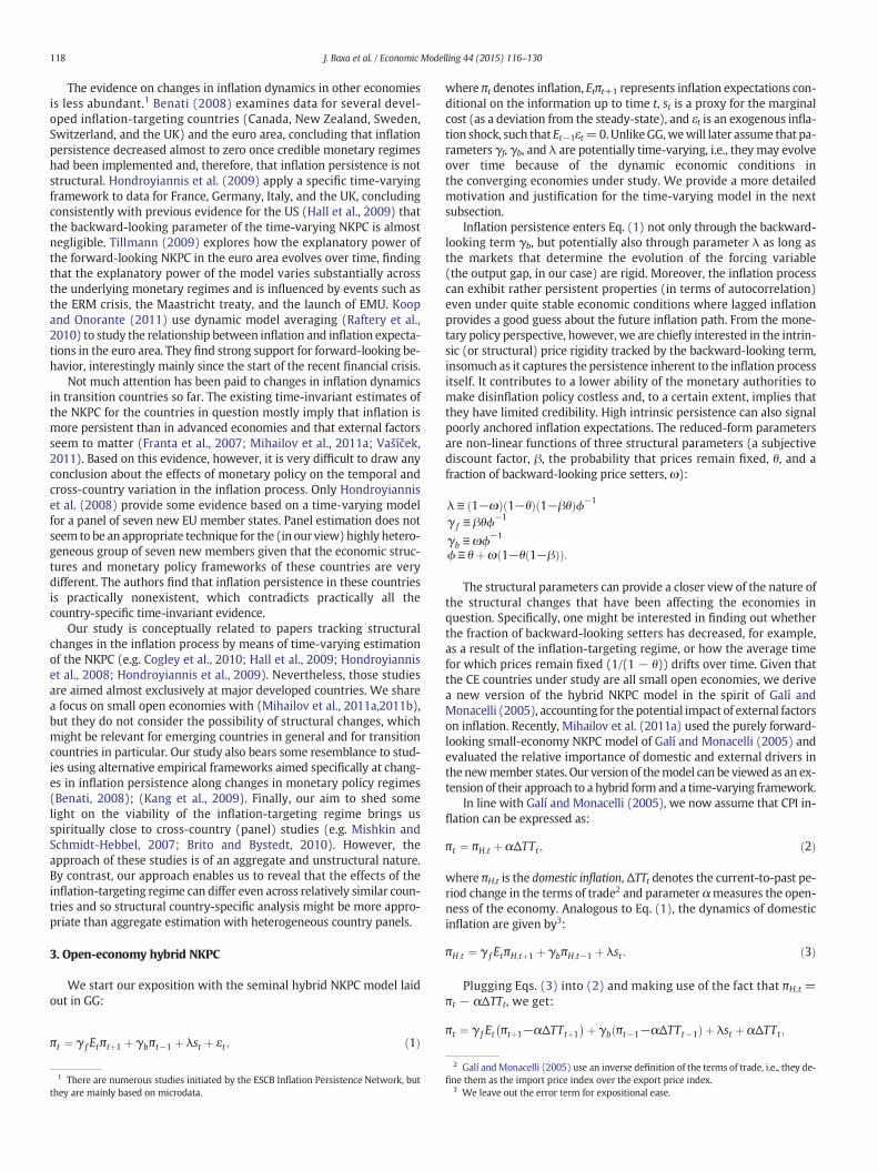
One way to check for parameter instability that is driven by smoothchanges (rather than abrupt breaks) is the method of flexible leastsquares (FLS, Kalaba and Tesfatsion, 1989). Although FLS is not aformal testing procedure it provides handy descriptive tools for analyz-ing variation in parameters. The objective function of the FLS estimatorconsists of two subcriteria, namely: the goodness-of-fit, determined bythe squared residuals (themeasurement error, RM2 ) and the smoothnessof the coefficients, given by the sum of their squared first differences(the dynamic error, RD2). The relative weight assigned to each criterionis regulated through smoothing constant μ. When μ equals one, no

variation in the parameters is allowed, the dynamic error equals zero,and the measurement error attains its maximum. By contrast, when μequals zero, one allows for maximum variation in the coefficients,which results in a perfectfit. One of theuseful outputs of FLS is the resid-ual efficiency frontier, which consists of all pairs of measurement anddynamic errors which are implied by μ and are compatible with theminimum value of the objective function. The residual efficiency fron-tiers for all the CE countries are shown in Fig. 1. Its shape suggeststhat there is systematic parameter instability in all three countries.This instability is most pronounced in the Czech Republic and ratherless marked in Poland and Hungary. This can be seen from the largedecrease in the measurement error once we allow for even a verysmall variation in the coefficients. At the same time, an inspection ofthe coefficients' paths for alternative values of the smoothing parameterreveals that gradual changes are a more plausible framework than thepresence of a single break.

Against this backdrop, in our empirical analysis we opt for anapproach which deals with the endogeneity problem similarly toGMM but can additionally tackle the issue of smooth parameter varia-tion. Since our approach also relies on the use of instruments and assuch may be prone to the same sensitivity to the choice of those instru-ments as the GMM estimator, we additionally use appropriate methodsto reduce the uncertainty in instrument selection.

4.1. Dealing with time variation and endogeneity

To overcome the problem of endogeneity in a time-varying frame-work we broadly stick to the strategy proposed by Kim (2006), whosuggests estimating a time-varying regression model with endogenousregressors by employing a two-step procedure. In the first step, oneruns an OLS regression9 of the endogenous variables on a set of instru-ments that are uncorrelated with the error term in Eq. (5). To finish the

first step we get residuals vt ¼ yt−yt , estimate Σv by Σv ¼ ∑Tt¼1

1Tvt v

0t ,

and obtain the standardized residuals v�t ¼ Σ−1=2v vt . These residuals

are used as the additional regressors in Eq. (5), where they serve asthe endogeneity correction terms. After insertion of the correctionterms into the NKPCmodel the whole systemwith time-varying coeffi-cients can be cast into the state-space form (see Subsection 4.3) andestimated using slightly modified Kalman filter formulas which correct

Fig. 1. Flexible least squares: residual efficiency frontier.

121J. Baxa et al. / Economic Modelling 44 (2015) 116–130

for bias in the variance of the estimated states. Full details are given inKim (2006) and Kim (2008).10

Despite the practical appeal of the two-step procedure of Kim(2006), we are still left with considerable uncertainty about whichinstruments should be used in the first-step OLS regression. Anotherproblem is that the standard estimation of linear state-spacemodels as-sumes constant Gaussian shocks to the target variable, which is unlikelyto hold for the inflation process (as argued, for example, in Koop andKorobilis, 2009). Applying methods that ignore possible variation inthe volatility of the error term in the NKPC model may lead to seriousbias of the estimated time-varying coefficients. Indeed, we find thatvarying volatility of shocks does matter and its omission leads to highlyerratic and unstable results.11

Based on these facts,we improve upon the original procedure of Kim(2006) and introduce some necessary modifications. Namely, weemploy Bayesian model averaging to select a proper set of instrumentsand use a stochastic volatility model for the error term in Eq. (5) toaccount for potential changes in the volatility of inflation shocks.12 Inthe following two subsections we provide a deeper justification foreach modification and give some technical details of our estimationapproach.

4.2. Instrument selection and Bayesian model averaging

As suggested by the GMM results in Table 1 models with rationalexpectations such as the NKPC are subject to considerable uncertaintyin instrument selection. Under these conditions, the Bayesian modelaveraging (BMA) provides a coherent framework to account for modeluncertainty and instrument sensitivity. It is a relatively new method(see Hoeting et al., 1999) that was introduced to a wider audience in

10 Note that we did not modify the variance of the states in our empirical exercise andour estimates of the time-varying parameters may thus be subject to higher uncertaintythan that presented in Section 5. The variance of the time-varying parameters dependson the (square) value of the estimated coefficient on the standardized residuals. Since inour case itwas usually quite small and statistically insignificant, the differences in the con-fidence intervals should mostly be negligible.11 Due to their apparent failure, we do not present these results here, but they are avail-able upon request.12 Although the (Kim, 2006) procedure in principle allows heteroskedasticity to be dealtwith by means of GARCH, the prevailing view in the literature is that stochastic volatilitymodels are more flexible and usually outperform ARCH-type models (Kim et al., 1998).

the mid-1990s. To our knowledge, BMA is new in the NKPC literature,although similar ideas have already been tossed around in the contextof rational expectations models (see Wright, 2003). Unlike the‘traditional’ approach to estimation of the NKPC, where a researchertypically selects instruments (and thus conditions her model) in quitea subjective manner, BMA effectively weights all the possible modelsbased on the posterior model probability. The relative importance ofeach instrument can be then inferred from its posterior inclusionprobability, which is equal to the sum of the posterior probabilitiesover the models in which it is included.

The application of BMA in our setting can be summarized as follows.Let Z be a T × k matrix of instruments containing the informationavailable to economic agents. Under standard assumptions, the unre-stricted model can be represented as:

yt ¼ aþ Ztδþ ϵt ϵ∼N 0;σ2� �

; ð6Þ

where yt denotes the outcome variable πt+1, a is an intercept, and δ is avector of parameters. Since economic theory leaves us rather agnosticabout the ‘true’ model, the researcher may have some uncertaintyoverwhich instruments to include or exclude. All possible combinationsof instruments form the model universe M = [M1, M2, …, MK], whereK = 2k. The BMA solution to the problem is to weight the outcomes ofall the models by their posterior probability. The fitted value ŷtBMA canthen be expressed as:

yBMAt ¼

XK

k¼1

yt;kp Mkjy; Zð Þ; ð7Þ

where ŷt,k denotes afitted value conditional on themodel k, andweightsp(Mk|y, Z) are the posterior model probabilities that arise from Bayes'theorem:

p Mkjy; Zð Þ ¼ p yjMk; Zð Þp Mkð Þp yjZð Þ ¼ p yjMk; Zð Þp Mkð ÞXK

s¼1p yjMs; Zð Þp Msð Þ

; ð8Þ

where p(y|Mk, Z) denotes themarginal likelihood of themodel, p(Mk) isthe prior probability that Mk is the ‘true’ model, and the denominatorrepresents the integrated likelihood, which is constant over the modeluniverse. The expressions for themarginal likelihood p(y|Mk, Z) dependon the problem at hand and vary across different kinds of models. In alinear regression setting, themarginal likelihood has a closed-formsolu-tion or can be obtained by approximation (depending on the nature of

122 J. Baxa et al. / Economic Modelling 44 (2015) 116–130

the priors on the coefficients).13 Before running BMA, the researcherneeds to specify the model universe (set of instruments), the modelpriors P(Mk), and the parameter priors P(ϖ|Mk), withϖ ≡ (a, δ ′, σ 2) ′.

In our setting, yt represents the endogenous variables in Eq. (5)14

and the instrument set includes four lags of inflation, the output gap,the unit labor cost, long-term interest rates, the interest rate spread, un-employment, the nominal effective exchange rate, and the crude oilprice. We aimed to include the most comprehensive set of instrumentsconsistently with previous papers, subject to data availability. We usethe hyper-g prior on the coefficients proposed by Liang et al. (2008)and run the Bayesian adaptive sampling algorithm (Clyde et al., 2011)to obtain the posterior probabilities over the models.

In light of our considerations above, it may also seem reasonable toaccount for the time-varying relation between the target (endogenous)variable and the instruments. Recently, Raftery et al. (2010) proposed anew method called dynamic model averaging (DMA) that accounts forboth model uncertainty and parameter variation. Since forecasting ex-ercises have shown that BMA and DMA perform comparably at shorthorizons (see Koop and Korobilis, 2009), and given that DMA is stillcomputationally unfeasible for large instrument sets, we regard BMAas a reasonable option for the first-step regression.15

4.3. The complete model

The hybrid NKPC in Eq. (5) with added correction terms, time-varying coefficients, and stochastic volatility can be cast into the follow-ing state-space representation (see Nakajima, 2011, for generalrepresentations of time-varying regression and VAR models withstochastic volatility):

πt ¼ c0tκ þ x0t f t þ ψt ; ψt∼N 0;σ2t

� �ð9Þ

f tþ1 ¼ f t þ ut ; ut∼N 0;Σð Þ ð10Þ

σ2t ¼ γexp htð Þ ð11Þ

htþ1 ¼ ρht þ ηt ; ηt∼N 0;σ2η

� �; ð12Þ

where ct ≡ (vt,π∗ , vt,gap∗ ) ′ is a vector of the endogeneity correction terms,xt≡ (πt+1, πt−1, st, TTt) ′ is a vector containing keymodel covariates, κ is avector of constant parameters, and ft≡ (γf,t,γb,t, λt,αt) ′ represents a vec-tor of time-varying coefficients.

The time-varying coefficients are constrained to follow a randomwalk, which allows for both permanent and transient shifts. Such aspecification is designed to capture gradual smooth changes and/orstructural breaks in the coefficients. Disturbances in Eq. (9), denotedψt, are normally distributed with time-varying variance σt

2. Thelog-volatility, ht = log(σt

2/γ), is modeled as an AR(1) process.

13 BMA for linear models has been implemented in several statistical products. Here, wemake use of the BAS package (Clyde et al., 2011), which is freely available in DevelopmentCore Team (2011).14 As we have shown above, the endogeneity problem enters the model through the re-placement of inflation expectationswith the observable value of future inflation. The forc-ing variable (the unit labor cost or the output gap) is usually considered exogenous.However, we believe that endogeneity of the output gap cannot be rejected a priori. Forthis reason, we formally treat the output gap as endogenous in the first-step regressionand test for the presence of endogeneity in the second step by inspecting the statistical sig-nificance of the coefficient on the endogeneity correction term. The terms of trade in allspecifications are considered exogenous. All other variables are predetermined since theyenter the equation with some lag.15 Note that DMA requires full enumeration of all models, which is memory and timeconsuming for K greater than, say, 220.

The system of Eqs. (9)–(12) forms a non-linear state-space modelwith state variables ft and ht. The presence of stochastic volatility(the source of the non-linearity) makes traditional estimation difficultbecause the likelihood function is intractable. However, Bayesian infer-ence is still possible and we can estimate the model efficiently usingMarkov chain Monte Carlo (MCMC) methods.16 Now the only remain-ing issue is how to estimate parameter αt on the linear combination ofthe terms of trade. Recall that the terms of trade enter in Eq. (5) as{ΔTTt− γfEtΔTTt+1− γbΔTTt−1}, whichmeans that they are dependenton the value of coefficients γf and γb, which are not known beforehand.To solve this issue we first estimate the closed-economy version of theNKPC and obtain the initial values of γf and γb. These are used to calcu-late the compound expression for the terms of trade. Then we estimatethe open-economy version in Eq. (5) and again obtain new values for γf

and γb, which may be used to recalculate the terms of trade. We repeatthese steps until all the parameter values converge.

To obtain the results, we drewM= 70,000 samples from the poste-rior distribution and discarded the first 50,000 samples as a burn-in pe-riod. Belowwe report the results for the default (quite loose) coefficientpriors implemented by Nakajima (2011) in his code. As a robustnesscheck we also experimented with other parameter settings in theprior densities, but the results do not seem to be severely affected bythe choice of prior. Nevertheless, the mixing properties of the Markovchain improved as the priors got tighter. To check for convergence, wecomputed inefficiency factors (Geweke, 1992), which measure howwell the Markov chain mixes. The inefficiency factors were usuallyquite low (below 50). Occasionally, however, they reached valuesclose to 100 for some coefficients. Despite this fact, it still implies thatwe get about M/100 = 200 uncorrelated samples, which is consideredenough for posterior inference (see Nakajima, 2011). As a robustnesscheck we also obtained the posterior distribution of the coefficients bysampling only every tenth draw, as this can reduce the potential auto-correlation in the chain. Results, however, remained almost identical.

As indicated above, one might also be interested in the structuralparameters of theNKPCmodel. However, it would be extremely difficultin practice to estimate them directly from a highly non-linear state-space model. Since under quite mild conditions there is one-to-onemapping between the reduced-form coefficients and the structuralparameters, we avoid direct estimation of the structural parametersand instead use a non-linear solver to obtain their value from themedian of the posterior distribution of the reduced-form coefficients.17

4.4. Data

Our dataset combines time series taken from several data sources(ECB, Eurostat, OECD, IMF, and national statistical offices). They weremainly downloaded from the E(S)CB data warehouse, which integratesseries collected by the key supranational data providers. We used sea-sonally adjusted (SA) data or performed our own adjustment basedon X12 ARIMAwhen SA series were not directly available and statisticaltests detected seasonality. Due to the limited data availability inducedby the transition from a command to a free-market economy we areforced to use a relatively short time span, running from 1996 Q1 to2010 Q4. One also has to take into account lower data quality —

especially at the beginning of the sample, as the statistical services inCE countries still faced some difficulties in meeting newly adoptedstatistical standards. In this respect, the results should be interpretedwith some caution.

In line with Galí andMonacelli (2005) the inflation rate is measuredas the annualized quarter-on-quarter (log) difference in the

16 Nakajima (2011) shows how to sample from the posterior distribution of coefficientsusing a Gibbs sampler and provides all the necessary computational details. See Nakajima(2011) also for the reference to his Ox and Matlab codes, which were (after some modifi-cations) used for the estimation.17 We fixed the subjective factor β to 0.99.

20 However, due to the non-linear relation between reduced-form and deep coefficients,this may still imply sizable changes in the deep parameters.21 For Poland, Lyziak (2003) and Orlowski (2010) document that inflation expectationsactually became anchored to the target path about 2 years after inflation targeting wasadopted.

123J. Baxa et al. / Economic Modelling 44 (2015) 116–130

harmonized index of consumer prices. To proxy the marginal cost westick to the output gap taken from the OECD Economic Outlook18 ratherthan the commonly usedunit labor cost (labor share of income, LIS). Thelatter measure performed rather poorly in the cross-correlationpre-analysis and in the pre-estimation exercise. The terms of tradeseries are calculated as the ratio of the import price index to the exportprice index as taken from the Eurostat database.

In addition to the lags of the variables described above, our initial in-strument set includes (four lags of) the unit labor cost, unemployment,the nominal effective exchange rate, the crude oil price, the long-terminterest rate, the interest rate spread, and the foreign (EU) inflationrate. The spread is defined as the difference between 3M and overnightinterbank interest rates.19 As noted above, the number of lags – four –corresponds to that in most previous studies (see for example Galíet al., 2005).

It is important to highlight that the inflation rate (especiallyfor Hungary and Poland), along with some other variables, shows aclear non-stationary pattern. Since it is not evident whether the non-stationarity is a result of the time-varying environment or is of an intrin-sic nature, we rendered inflation stationary by shortening the estima-tion period to 1999 Q1–2010 Q4 and re-estimated model (4). Giventhat the overall results remained largely identical we report theoutcomes for the longer time span only.

5. Results

5.1. Fitting inflation expectations

Unless a reliablemeasure of actual inflation expectations is available,most empirical studies on the NKPC assume that inflation expectationsare formed rationally. In practice, inflation expectations are proxied byregressing actual future inflation on the set of instruments containinglags of different variables (see Section 4.4 for a description of the full in-strument set). As explained above, Bayesian model averaging (BMA)becomes our vehicle for formally selecting the relevant instruments.By running BMA separately for each country, we assume that the deter-minants of inflation expectations can differ across the three countries.The R-squared of the models with the highest posterior probabilitywas around 0.8 for all three countries.

The results of the BMA are presented in Fig. 2. Thesefigures show theinclusion probabilities for each instrument and each country, with redbars indicating a posterior inclusion probability higher than 0.5. It canbe clearly seen that these inclusion probabilities are indeed countryspecific, reflecting differences in the predictability of inflation in theCE countries. In particular, the results show that in Hungary, wherethe central bank strongly considers exchange rate fluctuations whenmaking its monetary policy decisions (Vonnak, 2008), the foreignvariables dominate over the domestic ones.

A more detailed inspection of the results reveals that these differ-ences might be related to country-specific mechanisms for the forma-tion of inflation expectations. In the Czech Republic, domestic inflationand real economic activity have the highest inclusion probabilities andonly the fourth lag of inflation in the eurozone has an inclusion proba-bility higher than 0.5. In Hungary, we observe the opposite pattern,with the highest inclusion probabilities for the nominal effectiveexchange rate and other foreign variables and economic activity, whilethe lags of domestic inflation have inclusion probabilities lower than0.1. The results of the first step for Poland lie somewhere in betweenand the BMA selects both domestic and foreign variables. Fig. 2 alsoshows how the BMA estimates of future inflation track actual future in-flation. The BMA estimate tracks the long-term trend in inflation andalso some pronounced peaks in the inflation rate. Some of the spikes,

18 It seems to correspond by and large to the output gap obtained by the HP filter.19 We resort to this rather simplistic definition due to the limited availability of other in-terest rate data in the given period.

however, were evidently unexpected given the information availableto the agents. In this respect, the BMA estimates fit our intuition aboutinflation expectations in all three countries. It should be stressed thatconsistently with GG we focus on quarter-on-quarter changes in theprice level, whereas most surveys provide year-on-year inflation.

5.2. Open-economy NKPC with time-varying parameters

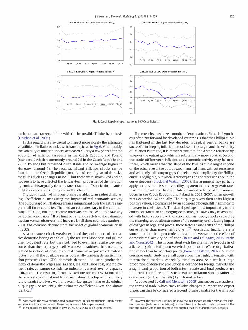
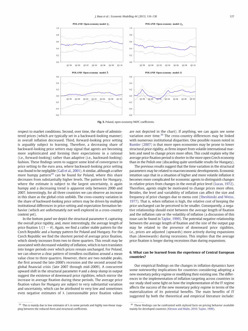
Figs. 3–5 present the estimated time-varying open economyreduced-form coefficients for the Czech Republic, Hungary, and Polandrespectively.

In general, we find evidence that the forward-looking inflation termis more important than the backward-looking one. This implies thatinflation expectations formed in forward-looking fashion play animportant role and are (at least partially) anchored in the CE countries.Consequently, monetary policy might be able to affect future inflationby influencing inflation expectations as such, for example by makinga credible commitment to future policy actions. However, thebackward-looking term,which arguably tracks intrinsic inflation persis-tence, remains largely significant (with a partial exception for the CzechRepublic). This is a somewhat different picture to that found in studiesfor developed countries that use a comparable econometric framework(e.g. Cogley et al., 2010; Hall et al., 2009). These studies usually arguethat a proper treatment of potential structural instabilities enables oneto fully abstract from the existence of intrinsic inflation persistence.

The small overall variation in the backward and forward-lookingcoefficients underlines their relative stability.20 However as usual,there are some exceptions to the rule which should not go unnoticed.Despite considerable uncertainty, as evidenced by the wide credibleintervals, one can occasionally observe that the median as well as thewhole posterior distribution tends to go downwards or upwards. Themost conspicuous instance is the decrease of the backward-lookingterm γb to practically insignificant levels in the Czech Republic. Corre-spondingly, the coefficient on the forward-looking term exhibits a slightupward tendency. A similar, albeit less pronounced, pattern can befound for Poland just until the outbreak of financial crisis. In 2008, theobserved resemblance seems to come to a halt. In the case of Hungaryboth coefficients are remarkably stable, showing only a mild decreasein the wake of the financial crisis.

Rather interestingly, we do not observe any peak or change in trendaround the time when inflation targeting was adopted (i.e., in 1998 inthe Czech Republic, in 1999 in Poland, and in 2001 in Hungary). Thisseems to imply that the shift to the new regime did not produce animmediate effect. However, we can observe some gradual changes inthe coefficients for the first two countries, with the already mentioneddrop in the backward-looking term 3 years after the implementationof inflation targeting in the Czech Republic.21 These changes wereaccompanied by an overall slump in the inflation rate below the infla-tion target in both countries. In the Czech Republic, the disinflationappeared shortly after the Czech National Bank decided to move fromperiodic setting of targets for the end of the year to continuous targetingof headline inflation within a predefined target range.22 The NationalBank of Poland originally set inflation targets in a similar manner as inthe Czech Republic, but during the first 2 years after IT implementationactual inflation ran well above the upper bounds of the announcedtargets. Inflation expectations were anchored to the inflation targets

22 Initially, the target was continuously decreasing, from 3–5% to 2–4% between 2002and 2005. However, since the inflation rate already often crawled below the inflation tar-get, the effects of the subsequent shift to point targets in 2005 and the change of thetargeted inflation rate from 3% to 2% in 2009 were negligible.

0.0

0.2

0.4

0.6

0.8

1.0

Mar

gina

l Inc

lusi

on P

roba

bilit

y

bas.lm(dependent ~ .)

Inte

rcep

tin

f_1

inf_

2in

f_3

inf_

4ga

p_1

gap_

2ga

p_3

gap_

4ul

c_1

ulc_

2ul

c_3

ulc_

4sp

read

_1sp

read

_2sp

read

_3sp

read

_4br

ent_

1br

ent_

2br

ent_

3br

ent_

4un

p_1

unp_

2un

p_3

unp_

4pr

ib_1

prib

_2pr

ib_3

prib

_4ne

er_1

neer

_2ne

er_3

neer

_4eu

_inf

_1eu

_inf

_2eu

_inf

_3eu

_inf

_4

Inclusion Probabilities BMA Inflation: CZ

1995 2000 2005 2010

−5

05

1015

20

Actual inflationBMA estimate

0.0

0.2

0.4

0.6

0.8

1.0

Mar

gina

l Inc

lusi

on P

roba

bilit

y

bas.lm(dependent ~ .)

Inte

rcep

tin

f_1

inf_

2in

f_3

inf_

4ga

p_1

gap_

2ga

p_3

gap_

4X

3Mra

te_1

X3M

rate

_2X

3Mra

te_3

X3M

rate

_4S

prea

d_1

Spr

ead_

2S

prea

d_3

Spr

ead_

4ne

er_1

neer

_2ne

er_3

neer

_4ul

c_1

ulc_

2ul

c_3

ulc_

4un

p_1

unp_

2un

p_3

unp_

4eu

_inf

_1eu

_inf

_2eu

_inf

_3eu

_inf

_4br

ent_

1br

ent_

2br

ent_

3br

ent_

4

Inclusion Probabilities BMA Inflation: HUN

2000 2005 2010

−5

05

1015

2025

Actual inflationBMA estimate

0.0

0.2

0.4

0.6

0.8

1.0

Mar

gina

l Inc

lusi

on P

roba

bilit

y

bas.lm(dependent ~ .)

Inte

rcep

tin

f_1

inf_

2in

f_3

inf_

4ga

p_1

gap_

2ga

p_3

gap_

4ul

c_1

ulc_

2ul

c_3

ulc_

4ne

er_1

neer

_2ne

er_3

neer

_4un

p_1

unp_

2un

p_3

unp_

4br

ent_

1br

ent_

2br

ent_

3br

ent_

4sp

read

_1sp

read

_2sp

read

_3sp

read

_4X

3Mra

te_1

X3M

rate

_2X

3Mra

te_3

X3M

rate

_4eu

_inf

_1eu

_inf

_2eu

_inf

_3eu

_inf

_4

Inclusion Probabilities BMA Inflation: POL

2000 2005 2010

−5

05

1015

2025

Actual inflationBMA estimate

Fig. 2. BMA results: posterior inclusion probabilities and model fit.

124 J. Baxa et al. / Economic Modelling 44 (2015) 116–130

shortly after the crawling peg was replaced with a pure float of thePolish zloty in April 2000.

On the contrary, the stability of the coefficients in Hungary prior tothe Great Recession is somewhat surprising given that, at least formally,the monetary policy framework has changed significantly over the pastyears.23 The main policy difference vis-à-vis the former two countrieslies arguably in the role attributed to the exchange rate (Vonnak,2008). Simultaneously with the shift to inflation targeting, the previouscrawling band exchange rate regime was replaced by a ‘shadow’ ERM IIregime of a fixed exchange rate with a fluctuation band of +/−15%

23 Inflation targets were announced at the end of the year for the following one until2007. A policy based on a predefined medium-term target (set at 3%) was implementedonly in 2008.

around the central parity against the euro (the other two countriesdid not declare any specific exchange rate target and maintained afree float for most of the time). Although this de facto meant the formaladoption of an exchange rate target (alongside the official inflation tar-get), theHungarian central bankwas not fully able to fulfill it in practiceand some inflationary depreciation periods followed.24 This is alsosupported by the fact that the exchange rate was identified as one ofthemost important factors of inflation expectations.With the evolutionof the coefficients inmind, this narrative evidence seems to suggest thatcontinuous targeting is a preferable vehicle for communicating mone-tary policy intentions and it seems preferable to disregard explicit

24 The most significant one in terms of its effect on inflation occurred in 2004, when in-flation increased from 3% to 7%.

0,0

0,2

0,4

0,6

0,8

1,0

Q1 98 Q1 00 Q1 02 Q1 04 Q1 06 Q1 08 Q1 10 -0,2

0,0

0,2

0,4

0,6

0,8

Q1 98 Q1 00 Q1 02 Q1 04 Q1 06 Q1 08 Q1 10

-0,4

-0,2

0,0

0,2

0,4

0,6

0,8

Q1 98 Q1 00 Q1 02 Q1 04 Q1 06 Q1 08 Q1 10

-0,6

-0,4

-0,2

0,0

0,2

0,4

0,6

0,8

Q1 98 Q1 00 Q1 02 Q1 04 Q1 06 Q1 08 Q1 10

Fig. 3. Czech Republic, open-economy NKPC coefficients.

125J. Baxa et al. / Economic Modelling 44 (2015) 116–130

exchange rate targets, in line with the Impossible Trinity hypothesis(Obstfeld et al., 2005).

In this regard it is also useful to inspect more closely the estimatedvolatilities of inflation shocks, which are depicted in Fig. 6.Most notably,the volatility of inflation shocks decreased quickly a few years after theadoption of inflation targeting in the Czech Republic and Poland(standard deviation commonly around 2.5 in the Czech Republic and2.0 in Poland) but remained quite stable and on average higher inHungary (around 4). The most significant inflation shocks can befound in the Czech Republic (mostly induced by administrativemeasures such as changes in VAT), but these were short-lived and donot seem to have affected the longer-term properties of the inflationdynamics. This arguably demonstrates that one-off shocks do not affectinflation expectations if they are well anchored.

The identification of inflation forcing variables turns rather challeng-ing. Coefficient λ, measuring the impact of real economic activity(the output gap) on inflation, remains insignificant over the entire sam-ple in all three countries. The median estimates vary in the commonrange of 0–0.2, but the credible intervals are too wide to draw anyparticular conclusion.25 If we limit our attention solely to the estimatedmedian,we can observe amild increase for all three countries starting in2001 and common decline since the onset of global economic crisisin 2008.

As a robustness check, we also explored the performance of alterna-tive domestic forcing variables: (i) the real unit labor cost, and (ii) theunemployment rate, but they both led to even less satisfactory out-comes than the output gap itself. Moreover, to address the uncertaintyrelated to individual measures of real economic output we estimated afactor from all the available series potentially tracking domestic infla-tion pressures (real GDP, domestic demand, industrial production,index of domestic wages and salaries, real unit labor cost, unemploy-ment rate, consumer confidence indicator, current level of capacityutilization). The resulting factor tracked the common variation of allthe series (besides real unit labor cost, whose development is entirelyidiosyncratic) relativelywell, andwas in fact quite similar to the originaloutput gap. Consequently, the estimated coefficient λ was also almostidentical.26

25 Note that in the conventional closed-economy set-up this coefficient is usually higherand significant for some periods. These results are available upon request.26 These results are not reported to save space, but are available upon request.

These results may have a number of explanations. First, the hypoth-esis often put forward for developed countries is that the Phillips curvehas flattened in the last few decades. Indeed, if central banks aresuccessful in keeping inflation rates close to the target and the volatilityof inflation is limited, it is rather difficult to find a stable relationshipvis-à-vis the output gap, which is substantially more volatile. Second,the trade-off between inflation and economic activity may be non-linear, which means that the slope of the Phillips curve might dependon the actual size of the output gap: in normal times without recessionsand with only mild output gaps, the relationship implied by the Phillipscurve is negligible, but when larger expansions or recessions occur, thecurve steepens (Stock and Watson, 2010). This argument may partiallyapply here, as there is some volatility apparent in the GDP growth ratesin all three countries. Themost blatant example relates to the economicboom in the Czech Republic and Poland in 2005–2007, when growthrates exceeded 6% annually. The output gap was then at its highestpositive values, accompanied by an apparent (though still insignificant)increase in coefficient λ. Third, and perhaps most importantly in thecontext of transition or emerging economies, the low λmay be associat-ed with factors specific to transition, such as supply shocks caused bythe changing production structure of the economy or the fading impactof changes in regulated prices. These factors cause shifts of the Phillipscurve rather than movement along it.27 Fourth and finally, there issome intuition that open trade and capital flows weaken the effect ofdomestic real activity on inflation (Razin and Loungani, 2005; Razinand Yuen, 2002). This is consistent with the alternative hypothesis ofa flattening of the Phillips curve, which points to the effects of globaliza-tion rather than to monetary policy (Borio and Filardo, 2007). All threecountries under study are small open economies highly integrated withinternational markets, especially the euro area. As a result, a largeproportion of domestic production is destined for foreign markets anda significant proportion of both intermediate and final products areimported. Therefore, domestic consumer inflation should rather bedetermined (at least partially) by external factors.

As advocated by Galí andMonacelli (2005) and subsequent authors,the terms of trade, which track relative changes in import and exportprices, can thus be considered a second forcing variable for the inflation

27 However, the first-step BMA results show that real factors are often relevant for infla-tion forecasts (inflation expectations). It may follow that the relationship between infla-tion and real drivers is actually more complicated than the standard NKPC suggests.

28 Thewhole distribution is obtained by calculating the structural coefficients from everyposterior draw of the reduced-form parameters.

0,0

0,2

0,4

0,6

0,8

1,0

Q1 98 Q1 00 Q1 02 Q1 04 Q1 06 Q1 08 Q1 10

0,0

0,2

0,4

0,6

0,8

1,0

Q1 98 Q1 00 Q1 02 Q1 04 Q1 06 Q1 08 Q1 10

-1,0

-0,6

-0,2

0,2

0,6

1,0

Q1 98 Q1 00 Q1 02 Q1 04 Q1 06 Q1 08 Q1 10

-1,0

-0,6

-0,2

0,2

0,6

1,0

Q1 98 Q1 00 Q1 02 Q1 04 Q1 06 Q1 08 Q1 10

Fig. 4. Hungary, open-economy NKPC coefficients.

126 J. Baxa et al. / Economic Modelling 44 (2015) 116–130

dynamics. However, the corresponding estimate of coefficient αt offersmixed evidence. A kind of trade-off between domestic and foreign infla-tion factors can be found in the Czech Republic, where foreign factorsdominate in the first half of the sample and domestic ones in the latter.For Poland, we find a predominance of foreign factors, with the corre-sponding coefficient αt being significant in several periods followinglarge depreciations (1997 Q4–1998 Q2, 2003 Q4–2004 Q3) and againat the onset of the late-2000's recession (2007 Q1–2008 Q2). ForHungary the estimated coefficient α is significantly negative on part ofthe sample. This goes against the underlying theory, but matches thefindings of Mihailov et al. (2011a).

A possible explanation of why the effects of external factors on infla-tion are only temporary (and possibly non-linear) might be that theyare already reflected in inflation expectations. If domestic firms engagein foreign trade, their inflation expectations are likely to be influencedby the exchange rate. For instance, in Hungary the exchange rate wason a depreciating path for the most of the time and thus arguablymade agents take future currency depreciation already into accountwhen forming their inflation expectations. Indeed in Hungary, theNEER turned out to be the most relevant variable in the first-step BMAresults, but the effect of external factors in Eq. (4) proved to be verylimited and disputable. By contrast, Poland experienced a few suddenand generally unexpected depreciation episodes (as noted above),which caused a huge temporary blip in its terms of trade with a signifi-cant impact on inflation.

As in the case of the domestic forcing variables we checked therobustness of our results using (i) the simple first difference of theterms of trade as well as their deviation from the HP-filtered trend,but the results based on the theoretical model are still preferable(as also found by Mihailov et al., 2011b), (ii) both the difference andthe deviations from the HP-trend of the NEER, but these variableswere generally insignificant.

5.3. Are the NKPC deep parameters truly structural?

While structural coefficients are routinely reported in papers basedon the time-invariant framework, time-varying studies do not usuallygo that far. The idea that the deep structural coefficients of the NKPCvary over time is rather controversial. However, macroeconomic devel-opments are inseparable from changes on the microeconomic level.When a change occurs in the macroeconomic setting, agents' behaviormight gradually adapt to the new conditions. In particular, recent

evidence suggests that firms' decisions on the frequency of priceadjustment are prone to be state-dependent (in contrast to the time-dependent pricing that is assumed by the NKPC). As corroborated bymostmicroeconomic studies on price setting, price adjustment ismainlyinfluenced by the level and variability of inflation (see Klenow andMalin, 2010, for a survey). Similarly, Fernandez-Villaverde and Rubio-Ramirez (2008) show within the DSGE framework that movements ofpricing parameters are indeed correlated with inflation. Therefore,there is no a priori reason why either the reduced-form or ‘structural’parameters of the NKPC should be time invariant.

This also seems to hold from a purely modeling perspective. Estrellaand Fuhrer (2003) and others offer a suite of methodological explana-tions of why structural models derived from agents' optimizing behav-ior and based on the assumption of rational expectations do notguarantee immunity to the Lucas critique. Therefore, the stability ofthe structural model and its ability to withstand the Lucas critiqueshould not be an a priori assumption, but should rather be a hypothesissubject to empirical testing. Arguably, the need to verify it is stronger intransition countries than anywhere else.

To check for potential instabilities, we reconstruct a sequence ofstructural coefficients from the reduced-form parameters,28 namely, i)the share of backward-looking price setters ω and ii) the average timefor which prices remain fixed as a function of θ. As already mentionedabove, the structural coefficients were derived under the assumptionthat the subjective factor, β, is fixed to 0.99. The results are reported inFig. 7. It is also important to note that since the estimates of λ are insig-nificant, one has to interpret the results with great caution. Moreover,for Hungary, the reduced-form coefficient of the output gap, λ, turnsnegative in some periods, and this impedes obtaining the structuralcoefficient θ in a reasonable range (these periods are dropped and thecorresponding coefficient series is discontinuous, although it still holdssome information).

In the upper panel we can see some differences in the share of ‘ruleof thumb’ firms, ω. The most economically consistent picture can bedrawn for the Czech Republic. The share of backward-looking firmsthat adjust prices simply to the inflation observed in the previous periodhas been slowly trending downwards. These developments correspondto our expectations. First, during the transition,firms faced continuouslyincreasing competition and needed to change their pricing policy with

0,0

0,2

0,4

0,6

0,8

1,0

Q1 98 Q1 00 Q1 02 Q1 04 Q1 06 Q1 08 Q1 10

0,0

0,2

0,4

0,6

0,8

1,0

Q1 98 Q1 00 Q1 02 Q1 04 Q1 06 Q1 08 Q1 10

-0,6

-0,4

-0,2

0,0

0,2

0,4

0,6

Q1 98 Q1 00 Q1 02 Q1 04 Q1 06 Q1 08 Q1 10

-0,6

-0,4

-0,2

0,0

0,2

0,4

0,6

Q1 98 Q1 00 Q1 02 Q1 04 Q1 06 Q1 08 Q1 10

Fig. 5. Poland, open-economy NKPC coefficients.

127J. Baxa et al. / Economic Modelling 44 (2015) 116–130

respect to market conditions. Second, over time, the share of adminis-tered prices (which are typically set in a backward-looking manner)in overall inflation decreased. Third, forward-looking price settingis arguably subject to learning. Therefore, a decreasing share ofbackward-looking price setters may signal that agents are becomingmore sophisticated and forming their expectations in a rational(i.e., forward-looking) rather than adaptive (i.e., backward-looking)fashion. These findings seem to suggest some kind of convergence inprice setting to the euro area, where backward-looking price settingwas found to be negligible (Galí et al., 2001). A similar, although a rathermore humpy pattern29 can be found for Poland, where this sharedecreases from substantially higher levels. The pattern for Hungary,where the estimate is subject to the largest uncertainty, is againhumpy and a decreasing trend is apparent only between 2000 and2007. Interestingly, for all three countries we can observe an increasein this share as the global crisis unfolds. The cross-country variation inthe share of backward-looking price setters may be driven by multipleinstitutional differences in price-setting and expectation formation be-havior (which are unfortunately not well explored in a cross-countrycontext yet).

In the bottom panel we depict the structural parameter θ, capturingthe overall price rigidity, and, more interestingly, the average length ofprice fixation 1/(1 − θ). Again, we find a rather stable pattern for theCzech Republic and a humpy pattern for Poland and Hungary. For theCzech Republic we find the shortest period of average price fixation,which slowly increases from two to three quarters. This result may beassociatedwith decreased volatility of inflation,which in turn translatesinto longer periods over which prices remain unchanged. For Poland,we can observe a clear pattern of trendless oscillation around a meanvalue close to three quarters. However, there are two notable peaks,the first around the late-2000's recession and the second around theglobal financial crisis (late 2007 through mid-2009). A concurrentupward shift in the structural parameter θ and a deep slump in outputsuggest the existence of downward price rigidities, which mirror theincrease in average fixation during these periods. The average pricefixation values for Hungary are subject to very substantial variationand uncertainty, which can be attributed to very low and sometimeseven negative estimates of λ (unreasonable price fixation values

29 This is mainly due to low estimates of λ in some periods and highly non-linear map-ping between the reduced-form and structural coefficients.

are not depicted in the chart). If anything, we can again see somevariation over time.30 The cross-country differences may be linkedwith numerous institutional disparities. One possible reason noted inRumler (2007) is that more open economies may be prone to lowerstructural price rigidity, as firms import from volatile international mar-kets and need to change prices more often. This could explain why theaverage price fixation period is shorter in themore open Czech economythan in the Polish one (discarding quite unreliable results for Hungary).

The previous results suggest that the time variation in the structuralparametersmay be related tomacroeconomic developments. Economicintuition says that in a situation of higher and more volatile inflation itbecomes more complicated for economic agents to distinguish changesin relative prices from changes in the overall price level (Lucas, 1972).Therefore, agents might be motivated to change prices more often.Besides, the level and variability of inflation can affect the size andfrequency of price changes due to menu cost (Sheshinski and Weiss,1977). That is, when inflation is high, the relative cost of keeping theprice unchanged can be perceived to be smaller. Consequently, a nega-tive relationship should exist between the average length of fixationand the inflation rate or the volatility of inflation (a discussion of thisissue can be found in Taylor, 1999). The potential negative relationshipbetween the average length of fixation and the size of the output gapmay be related to the presence of downward price rigidities,i.e., prices are adjusted (upwards) more actively during expansionsthan (downwards) during recessions. This implies that the averageprice fixation is longer during recessions than during expansions.

6. What can be learned from the experience of Central Europeancountries?

Our empirical findings on the changes in inflation dynamics havesome noteworthy implications for countries considering adopting anewmonetary policy regime ormodifying their existing one. The differ-ences in the implementation of inflation targeting across countries inour study shed some light on how the implementation of the IT regimeaffects the success of the new monetary policy regime in terms of thematerialization of its potential benefits. The main benefits of ITsuggested by both the theoretical and empirical literature include:

30 These findings can be confronted with stylized facts on pricing behavior availablemainly for developed countries (Klenow and Malin, 2010; Taylor, 1999).

0

5

10

15

20

25

30

35

Q1 98 Q1 00 Q1 02 Q1 04 Q1 06 Q1 08 Q1 10

CZECH REPUBLIC

0

1

2

3

4

5

6

Q1 98 Q1 00 Q1 02 Q1 04 Q1 06 Q1 08 Q1 10

POLAND

0

1

2

3

4

5

Q1 98 Q1 00 Q1 02 Q1 04 Q1 06 Q1 08 Q1 10

HUNGARY

Fig. 6. Stochastic volatility.

128 J. Baxa et al. / Economic Modelling 44 (2015) 116–130

(i) moderation of the level and volatility of inflation (Abo-Zaid andTuzemen, 2012; Goncalves and Salles, 2008; Svensson, 1997),(ii) anchoring of inflation expectations (Blinder et al., 2008), and(iii) increased transparency and credibility of monetary policy and thusreduced costs of disinflation (Batini and Laxton, 2007; Mishkin, 1999).

In general, the implementation of the IT framework as a disinflationstrategy proved to be successful (to some degree, at least) in all threecountries, since their high inflation rates dropped to lower levels shortlyafter its adoption.However, as far as the volatility of inflation shocks andthe credibility of the target are concerned, the three central banks seemto have met this goal with varying success. Whereas an overall reduc-tion of the inflation level has been achieved in all three CE countries, adecrease in inflation volatility can only be observed for the CzechRepublic and Poland, where the spikes in inflation volatility are rathershort-lived and realized inflationary shocks dissipate quite quickly. Con-sequently, the link between (temporarily) higher volatility of inflationand increasing persistence seems to have been broken as well. Themost significant decrease in inflation persistence has been recorded in

0

0,1

0,2

0,3

0,4

0,5

0,6

0,7

Q1 98 Q1 00 Q1 02 Q1 04 Q1 06 Q1 08 Q1 10

CZECH REPUBLIC: ω

Median Lower and Upper Quartile

0

0,2

0,4

0,6

0,8

1

1,2

Q1 98 Q1 00 Q1 02 Q1

POLAND:

Median Lowe

2

3

4

5

0,2

0,4

0,6

0,8

1

Q1 98 Q1 00 Q1 02 Q1 04 Q1 06 Q1 08 Q1 10

CZECH REPUBLIC: θ

Avg. price fixation (right axis)

0,2

0,4

0,6

0,8

1

1,2

Q1 98 Q1 00 Q1 02 Q1 0

POLAND

Avg. price fixatio

Note: Structural coefficients for Hungary ar

Fig. 7. Estimates of deep parameters. Note: structural coefficien

the Czech Republic, where it has been accompanied by anchoring ofinflation expectations. As a result, the Czech inflation process seems tobe drivenmainly by its forward-looking component. By contrast, signif-icant inflation persistence has remained an important phenomenon inboth Hungary and Poland, suggesting that past inflation bears relevantinformation for the formation of inflation expectations. Moreover,Hungary does not even have an observable pattern of reduced inflationpersistence.

Although even ex post it is not fully clear whether the observedchanges in inflation dynamics can be wholly attributed to inflationtargeting, the fact that the changes occurred shortly after the adoptionof the IT regime, and that the differences in IT implementation in thethree CE countries match the observed differences in inflation dynam-ics, suggests that IT played a considerable role. Whereas the CzechRepublic and Poland seem, according to several characteristics, toadhere to full-fledged inflation targeting, the monetary policy ofHungary in most categories can be characterized as inflation targetinglite (using the IT typology classification of Carare and Stone, 2006, see

04 Q1 06 Q1 08 Q1 10

ω

r and Upper Quartile

0

0,2

0,4

0,6

0,8

1

Q1 98 Q1 00 Q1 02 Q1 04 Q1 06 Q1 08 Q1 10

HUNGARY: ω

Median Lower and Upper Quartile

2

3

4

5

4 Q1 06 Q1 08 Q1 10

: θ

n (right axis)

2

3

4

5

6

7

0,2

0,4

0,6

0,8

1

1,2

Q1 98 Q1 00 Q1 02 Q1 04 Q1 06 Q1 08 Q1 10

HUNGARY: θ

Avg. price fixation (right axis)

e dropped for periods when λ is negative.

ts for Hungary are dropped for periods when λ is negative.

Table 3Varieties of inflation-targeting regimes and realized outcomes.

Czech Republic Poland Hungary

Clarity of commitment to inflation target Main objective is price stability Main objective is price stability Main objective is price stabilityNumeric value of target 2% ± 1 pp 2.5% ±1 pp 3%Definition of target and evaluation of fulfillment Continuous, without pre-defined

date of revisionContinuous, without pre-defineddate of revision

Continuous, medium-term target,reassessed after 3–5 years

Exchange rate regime Managed float Free float Crawling bandCredibility: past departures from target Short-term, both positive and

negative deviationsShort-term, both positive andnegative deviations

Persistently above target, deviationsexceed 2%

Average inflation (before/after 2003) 5.17%/2.7% 8.56%/2.72% 10.98%/5.1%Moderation of inflation level Yes Yes YesInflation volatility: average of 3-year standard

deviation (before/after 2001)3.76/2.39 3.63/1.85 3.09/2.74

Moderation of inflation volatility Yes Yes NoCredibility: S&P sovereign domestic-currencyrating since IT implementation

A to AA A A to BB

Note: The table shows the dominantmonetary policy characteristics over the years of IT and themean values of variables proxying the key IT outcomes. However, both the characteristicsand outcomes of the IT regime changed over time.

129J. Baxa et al. / Economic Modelling 44 (2015) 116–130

Table 3 for details). Most notably, the Czech and Polish numericalinflation targets are lower and are continuously assessed, and thesecountries' policy track records show better target fulfillment. Last butnot the least, the exchange rates of the Czech koruna and Polish zlotyhave floated freely most of the time. On the contrary, in Hungary wedo not observe major changes in inflation dynamics after the adoptionof inflation targeting, and the expected positive effects of the IT regime(e.g. lower inflation volatility, reduced inflation persistence, andincreased credibility) did not materialize. The narrative record ofHungarian monetary policy suggests that several aspects of the imple-mentation of inflation targeting undermined the credibility of thetarget. In particular, although inflation targeting should be aimed atthe domestic price level, Hungarian monetary policy has paid specialattention to the exchange rate and the exchange rate channel is consid-ered the most efficient channel of monetary policy transmission(Vonnak, 2008). This policy choice has had its costs in terms of regimecredibility, as the inflation target has often been missed. This seems toreflect the Impossible Trinity of simultaneously stabilizing domesticinflation and hitting the exchange rate target in the presence of freecapital flows. Consequently, the prevailing inflation rates in Hungarydid not allow for a significant reduction in interest rates, and the highinterest rate differential between the Hungarian forint and othercurrencies drove a significant expansion of foreign currency lending,which ultimately turned into a severe financial stability problem.

These conclusions support the view of (e.g. Mishkin and Schmidt-Hebbel, 2007) that inflation-targeting countries do not necessarily per-form better (in terms of either output or inflation volatility) than thosethat do not target inflation. Based on panel data methods, they arguethat what seems to matter the most is the establishment of a strongnominal anchor and the anchoring of inflation expectations. Benati(2008) also points to credibility rather than to a particular monetarypolicy regime as such. The time series view of three rather homoge-neous CE countries with minor but important differences in policydesign clearly demonstrates that these differences matter. From thisperspective, the key policy objective of lowering the inflation levelwas met and the policy can be seen as successful. However, taking abroader view and other objectives on board, the assessment of theperformance of the IT regime is more equivocal across countries. Theresults confirm that the adoption of the IT framework does not automat-ically go hand in hand with building credible and transparent policy,and these challenges become even more striking when maintaininginflation at the targeted value is not the only monetary policy objective.

7. Conclusions

This paper aims to shed some light on possible changes in inflationdynamics in the presence of structural changes in the economy and

the monetary policy regime. It analyzes the dynamics of inflationthrough the lens of the New Keynesian Phillips curve nested within atime-varying framework using data for three CE countries. Althoughoriginally the NKPC was proposed as a structural model of inflationdynamicswhich is invariant to policy changes, it is likely that substantialchanges on the macroeconomic level coupled with large-scalerestructuring of whole economies also resulted in significant changesat the microeconomic level.

In general, we find that the considerable structural changes experi-enced by the economies under study, coupled with shifts in their mon-etary regimes, produced some notable changes in the inflation process.However, the nature of those changes is still rather heterogeneousacross countries — despite their relative regional and historical affinity.Our results imply that the adoption of inflation targeting per se does notguarantee desirable outcomes such as a reduction in intrinsic inflationpersistence or inflation volatility. The implementation details mightmatter as well, supporting the need for a structural country-levelanalysis.

As regards the cross-country differences, we found that intrinsic in-flation persistence decreased substantially in the Czech Republic only.This implies that lower inflation can be achieved by anchoring inflationexpectations and is not necessarily accompanied by output or employ-ment losses. These findings are supported by the estimated volatilityof inflation shocks, which decreased quickly a few years after the adop-tion of inflation targeting in the Czech Republic and also in Poland.Indeed, the predominantly forward-looking nature of the inflationprocess and the short-lived inflation shocks point to well-anchoredinflation expectations. By contrast, almost all the characteristics describ-ing the inflation process in Hungary are surprisingly stable. In ouropinion, the comparatively low impact of the introduction of inflationtargeting on inflation dynamics may be associated with the significantrole of the exchange rate in Hungarian monetary policy.

The overall changes in the inflation process can be traced to changesin microeconomic behavior, in particular the price-setting behavior offirms.We found some evidence that the ‘structural’ coefficients describ-ing this behavior are stable neither over time nor in the cross-sectionaldimension. While the time variation can be related to the macroeco-nomic environment, the cross-country variation can be linked to institu-tional differences determining the nature of price-setting behavior andexpectation formation.

References

Abo-Zaid, S., Tuzemen, D., 2012. Inflation targeting: a three-decade perspective. J. PolicyModel 34 (5), 621–645.

Ball, L.M., Sheridan, N., 2004. Does inflation targeting matter? The Inflation-TargetingDebate. University of Chicago Press, pp. 249–282.

130 J. Baxa et al. / Economic Modelling 44 (2015) 116–130

Batini, N. and Laxton, D. (2007). Under What Conditions Can Inflation Targeting BeAdopted? The Experience of Emerging Markets. In Miskin, F. S., Schmidt-Hebbel, K.,Editor), N. L. S., and (Se, K. S.-H., editors, Monetary Policy under Inflation Targeting,volume 11 of Central Banking, Analysis, and Economic Policies Book Series, chapter 12,pages 467–506. Central Bank of Chile.

Batini, N., Jackson, B., Nickell, S., 2005. An open-economy new Keynesian Phillips curve forthe U.K. J. Monet. Econ. 52 (6), 1061–1071.

Benati, L., 2008. Investigating inflation persistence across monetary regimes. Q. J. Econ.123 (3), 1005–1060.

Blinder, A.S., Ehrmann, M., Fratzscher, M., Haan, J.D., Jansen, D.-J., 2008. Central Bankcommunication and monetary policy: a survey of theory and evidence. J. Econ. Lit.46 (4), 910–945.

Borio, C., Filardo, A., 2007. Globalisation and Inflation: New Cross-country Evidence on theGlobal Determinants of Domestic Inflation.

Brito, R.D., Bystedt, B., 2010. Inflation targeting in emerging economies: panel evidence.J. Dev. Econ. 91 (2), 198–210.

Carare, A., Stone, M.R., 2006. Inflation targeting regimes. Eur. Econ. Rev. 50 (5),1297–1315.

Clyde, M., Ghosh, J., Littman, M., 2011. Bayesian adaptive sampling for variable selectionand model averaging. J. Comput. Graph. Stat. 20 (1), 80–101.

Cogley, T., Sbordone, A.M., 2008. Trend inflation, indexation, and inflation persistence inthe new Keynesian Phillips curve. Am. Econ. Rev. 98 (5), 2101–2126.

Cogley, T., Primiceri, G.E., Sargent, T.J., 2010. Inflation-gap persistence in the US. Am. Econ.J. Macroecon. 2 (1), 43–69.

Davig, T., Doh, T., 2008. Monetary Policy Regime Shifts and Inflation Persistence. FederalReserve Bank of Kansas City, (Research working paper).

Development Core Team, R., 2011. R: A Language and Environment for StatisticalComputing. R Foundation for Statistical Computing, Vienna, Austria 3-900051-07-0.

Estrella, A., Fuhrer, J.C., 2003. Monetary policy shifts and the stability of monetary policymodels. Rev. Econ. Stat. 85 (1), 94–104.

Fernandez-Villaverde, J., Rubio-Ramirez, J.F., 2008. How structural are structural parameters?NBER Macroeconomics Annual 2007 vol. 22. National Bureau of Economic Research,Inc., pp. 83–137 (NBER Chapters).

Franta, M., Saxa, B., Šmídková, K., 2007. Inflation Persistence — Euro Area and New EUMember States. European Central Bank, (Working Paper Series 810).

Galí, J., Gertler, M., 1999. Inflation dynamics: a structural econometric analysis. J. Monet.Econ. 44 (2), 195–222.

Galí, J., Monacelli, T., 2005. Monetary policy and exchange rate volatility in a small openeconomy. Rev. Econ. Stud. 72 (3), 707–734.

Galí, J., Gertler, M., Lopez-Salido, J.D., 2001. European inflation dynamics. Eur. Econ. Rev.45 (7), 1237–1270.

Galí, J., Gertler, M., Lopez-Salido, J.D., 2005. Robustness of the estimates of the hybrid newKeynesian Phillips curve. J. Monet. Econ. 52 (6), 1107–1118.

Geweke, J., 1992. Evaluating the accuracy of sampling-based approaches to thecalculation of posterior moments (with discussion). Bayesian Stat. 4, 169–193.

Goncalves, C.E.S., Salles, J.M., 2008. Inflation targeting in emerging economies: what dothe data say? J. Dev. Econ. 85 (1–2), 312–318.

Hall, S.G., Hondroyiannis, G., Swamy, P.A.V.B., Tavlas, G.S., 2009. The new KeynesianPhillips curve and lagged inflation: a case of spurious correlation? South. Econ. J.76 (2), 467–481.

Hoeting, J.A., Madigan, D., Raftery, A.E., Volinsky, C.T., 1999. Bayesian model averaging: atutorial. Stat. Sci. 14 (4), 382–417.

Hondroyiannis, G., Swamy, P., Tavlas, G.S., 2008. Inflation dynamics in the euro area and innew eu members: implications for monetary policy. Econ. Model. 25 (6), 1116–1127.

Hondroyiannis, G., Swamy, P., Tavlas, G.S., 2009. The new Keynesian Phillips curve in atime-varying coefficient environment: some European evidence. Macroecon. Dyn.13 (02), 149–166.

Kalaba, R., Tesfatsion, L., 1989. Time-varying linear regression via flexible least squares.Comput. Math. Appl. 17 (8), 1215–1245.

Kang, K.H., Kim, C.-J., Morley, J., 2009. Changes in U.S. inflation persistence. Stud.Nonlinear Dyn. Econom. 13 (4), 1.

Kim, C.-J., 2006. Time-varying parameter models with endogenous regressors. Econ. Lett.91 (1), 21–26.

Kim, C.-J., 2008. Dealing with endogeneity in regression models with dynamiccoefficients. Found. Trends Econom. 3 (3), 165–266.

Kim, S., Shephard, N., Siddhartha, Ch., 1998. Stochastic Volatility: Likelihood Inference andComparison with ARCH Models. Rev. Econ. Stud. 65 (3), 361–393.

Klenow, P.J., Malin, B.A., 2010. Microeconomic evidence on price-setting. In: Friedman,B.M., Woodford, M. (Eds.), Handbook of Monetary EconomicsHandbook of MonetaryEconomics vol. 3. Elsevier, pp. 231–284 (chapter 6).

Koop, G., Korobilis, D., 2009. Forecasting Inflation Using Dynamic Model Averaging.Rimini Centre for Economic Analysis, (Working Paper Series 34–09).

Koop, G., Onorante, L., 2011. Estimating Phillips curves in turbulent times using the ECBssurvey of professional forecasters. Department of Economics. University ofStrathclyde Business School (Working Papers 1109).

Liang, F., Paulo, R., Molina, G., Clyde, M.A., Berger, J.O., 2008. Mixtures of g priors forBayesian variable selection. J. Am. Stat. Assoc. 103 (481), 410–423.

Lindé, J., 2005. Estimating new-Keynesian Phillips curves: a full information maximumlikelihood approach. J. Monet. Econ. 52 (6), 1135–1149.

Lucas, R.E., 1972. Expectations and the neutrality of money. J. Econ. Theory 4 (2),103–124.

Lyziak, T., 2003. Consumer Inflation Expectations in Poland. European Central Bank,(Working Paper Series 287).

Mavroeidis, S., 2005. Identification issues in forward-looking models estimated by GMM,with an application to the Phillips curve. J. Money Credit Bank. 37 (3), 421–448.

Mavroeidis, S., Plagborg-Møller, M., Stock, J.H., 2013. Empirical Evidence on InflationExpectations in the New Keynesian Phillips Curve.

Mihailov, A., Rumler, F., Scharler, J., 2011a. Inflation dynamics in the new EU memberstates: how relevant are external factors? Rev. Int. Econ. 19 (1), 65–76.

Mihailov, A., Rumler, F., Scharler, J., 2011b. The small open-economy new KeynesianPhillips curve: empirical evidence and implied inflation dynamics. Open Econ. Rev.22 (2), 317–337.

Mishkin, F.S., 1999. International experiences with different monetary policy regimes.J. Monet. Econ. 43 (3), 579–605.

Mishkin, F.S., Schmidt-Hebbel, K., 2007. Does inflation targeting make a difference?National Bureau of Economic Research, (Technical report).

Nakajima, J., 2011. Time-varying parameter VAR model with stochastic volatility:an overview of methodology and empirical applications. Imes discussion paperseriesInstitute for Monetary and Economic Studies, Bank of Japan.

Obstfeld, M., Shambaugh, J.C., Taylor, A.M., 2005. The trilemma in history: tradeoffsamong exchange rates, monetary policies, and capital mobility. Rev. Econ. Stat. 87(3), 423–438.

Orlowski, L.T., 2010. Monetary policy rules for convergence to the euro. Econ. Syst. 34 (2),148–159.

Primiceri, G.E., 2005. Time varying structural vector autoregressions and monetary policy.Rev. Econ. Stud. 72 (3), 821–852.

Raftery, A., Kárny, M., Ettler, P., 2010. Online prediction under model uncertainty viadynamic model averaging: application to a cold rolling mill. Technometrics 52,52–66.

Razin, A., Loungani, P., 2005. Globalization and Inflation–Output Tradeoffs. NationalBureau of Economic Research, Inc., (NBER Working Papers 11641).

Razin, A., Yuen, C.-W., 2002. The ‘new Keynesian’ Phillips curve: closed economy versusopen economy. Econ. Lett. 75 (1), 1–9.

Rudd, J., Whelan, K., 2005. New tests of the new-Keynesian Phillips curve. J. Monet. Econ.52 (6), 1167–1181.

Rumler, F., 2007. Estimates of the open economy new Keynesian Phillips curve for euroarea countries. Open Econ. Rev. 18 (4), 427–451.

Sheshinski, E., Weiss, Y., 1977. Inflation and costs of price adjustment. Rev. Econ. Stud. 44(2), 287–303.

Stock, J.H., Watson, M.W., 2007. Why has U.S. inflation become harder to forecast?J. Money Credit Bank. 39 (s1), 3–33.

Stock, J.H., Watson, M.W., 2010. Modeling Inflation after the Crisis. National Bureau ofEconomic Research, Inc., (NBER Working Papers 16488).

Svensson, L.E.O., 1997. Inflation forecast targeting: implementing and monitoringinflation targets. Eur. Econ. Rev. 41 (6), 1111–1146.

Taylor, J.B., 1999. Staggered price and wage setting in macroeconomics. In: Taylor, J.,Woodford, M. (Eds.), Handbook of MacroeconomicsHandbook of Macroeconomicsvol. 1. Elsevier, pp. 1009–1050 (chapter 15).

Tillmann, P., 2009. A note on the stability of the new Keynesian Phillips curve in Europe.Appl. Econ. Lett. 17 (3), 241–245.

Vašíček, B., 2011. Inflation dynamics and the new Keynesian Phillips curve in EU-4.Emerg. Mark. Finance Trade 47 (5), 71–100.

Vonnak, B., 2008. The Hungarian monetary transmission mechanism: an assessment. In:International Settlements, B (Ed.), Transmission mechanisms for monetary policy inemerging market economiesBIS Papers chapters vol. 35. Bank for InternationalSettlements, pp. 235–257.

Wright, J.H., 2003. Forecasting U.S. inflation by Bayesian model averaging. InternationalFinance Discussion Papers 780Board of Governors of the Federal Reserve,System (U.S.).

Zhang, Chengsi, D. R. O, Kim, D.H., 2008. The new Keynesian Phillips curve: from stickyinflation to sticky prices. J. Money Credit Bank. 40 (4), 667–699.