changing mass applications in an advanced time domain ship
TRANSCRIPT

Changing Mass Applications in an Advanced Time Domain
Ship Motion Program
by
Paul Richard Wynn
B.S., Virginia Tech (1986)
Submitted to the Department of Ocean Engineeringin partial fulfillment of the requirements for the degree of
Naval Engineer
at the
MASSACHUSETTS INSTITUTE OF TECHNOLOGY
June 2000
o 2000 Paul R. Wynn. All rights reserved.
The author hereby grants to MIT permission to reproduceand to distribute publicly paper and electronic
copies of this thesis document in whole or in part.
Signature of Author ............ ..... ..........................Department of Ocean Engineering
22 May 2000
C ertified by ........... .......................Dick K.P. Yue
Professor of Hydrodynamics and Ocean EngineeringThesis Supervisor
A ccepted by ........... .........................Nicholas M. Patrikalakis
Kawasaki Professor of EngineeringMASSACHUSETTS I STITUTE Chairman, Committee on Graduate Students
OF TECHNOLOGY Department of Ocean Engineering
NOV 2 9 2000ENILIBRARIES

Changing Mass Applications in an Advanced Time Domain Ship Motion
Program
by
Paul Richard Wynn
Submitted to the Department of Ocean Engineeringon 22 May 2000, in partial fulfillment of the
requirements for the degree ofNaval Engineer
Abstract
Models are developed for a state-of-the-art time-domain ship motion program to predict shipmotions during flooding and green water on deck events. Water mass from the flooding andgreen water is incorporated into the dynamic equations of motion using time-dependent massand moment of inertia terms.
Green water on deck includes three subproblems: the problem of water shipping on deck,the problem of motion of water trapped on the deck, and the problem of water escaping offthe deck. This research looks at the first two suproblems, both of which involve shallow waterwave theory. Glimms method, also called the Random Choice Method, and the Flux DifferenceSplitting Method are both investigated as solution techniques for the motion of water on deck.
This work provides a tool to estimate ship damaged stability and examine the effects ofprogressive flooding.
Thesis Supervisor: Dick K.P. YueTitle: Professor of Hydrodynamics and Ocean Engineering
2

Contents
1 Introduction
1.1 Background . . . . . . . . . . . . . . . . . . . . . . . . . . . . . .
1.2 Research Objectives . . . . . . . . . . . . . . . . . . . . . . . . .
2 LAMP Description and Development of Equations of Motion
2.1 LAM P Description . . . . . . . . . . . . . . . . . . . . . . . . . .
2.2 LAMP Rigid Body Dynamics . . . . . . . . . . . . . . . . . . . .
2.3 LAMP Rigid Body Dynamics With Time-Dependent Mass. . . .
2.3.1 Infinite Frequency Added Mass and Moment of Inertia . .
2.3.2 Translation: . . . . . . . . . . . . . . . . . . . . . . . . . .
2.3.3 Rotation: ...... ...........................
2.3.4 Coupled Rotation and Translation Equations: . . . . . . .
3 Models for Flooding
3.1 Compartmentation . . . . . . . . . . . . . . . . . . . . . . . . . .
3.2 Calculations For a Compartment's Flooded Volume . . . . . . . .
3.3 Flooding Simulation . . . . . . . . . . . . . . . . . . . . . . . . .
3.4 W ind . . . . . . . . . . . . . . . . . . . . . . . . . . . . . . . . . .
3.5 Causes of Loss of Accuracy in LAMP Flooding Simulations . . .
4 Models for the Green Water Problem
4.1 Background and Scope of Green Water Model . . . . . . . . . . .
4.2 Flux Difference Splitting Method for Water Motion on Deck . . .
8
. 8
. . . . . . . . . 10
12
12
17
19
19
20
21
23
24
. . . . . . . 24
. . . . . . . 26
. . . . . . . 28
. . . . . . . 29
. . . . . . . 29
31
31
32
3

4.3 Glimms Method (Random Choice Method) for Water Motion on Deck
4.3.1 Solution of the Riemann Problem . . . . . . . . . . . . . . . . .
4.4 Selection of Water Motion on Deck Method . . . . . . . . . . . . . . .
4.5 Water Shipping Model . . . . . . . . . . . . . . . . . . . . . . . . . . .
4.5.1 Free Surface Elevation for Water Shipping . . . . . . . . . . .
4.5.2 Relative Velocity for Water Shipping . . . . . . . . . . . . . . .
4.6 Green Water Model in LAMP . . . . . . . . . . . . . . . . . . . . . . .
. . . . . . 36
. . . . . . 37
. . . . . . 42
. . . . . . 43
. . . . . . 45
. . . . . . 46
. . . . . . 48
5 Validation and Results
5.1 Validation . . . . . . . . . . . . . . . . . . . . . . . . . . . . . . .
5.1.1 Validation of Dynamic Equation of Motion Solver . . . .
5.1.2 Validation of Compartment Flooded Volume and Moment
culation . . . . . . . . . . . . . . . . . . . . . . . . . . . .
5.1.3 Validation of Flux Difference Splitting Method . . . . . .
5.2 Results for Flooding Models . . . . . . . . . . . . . . . . . . . . .
5.2.1 Roll Motion Results . . . . . . . . . . . . . . . . . . . . .
5.2.2 Vertical Motion Results . . . . . . . . . . . . . . . . . . .
5.2.3 Loss of Accuracy Examples . . . . . . . . . . . . . . . . .
5.2.4 Progressive Flooding Results . . . . . . . . . . . . . . . .
5.3 Results for Green Water . . . . . . . . . . . . . . . . . . . . . . .
52
52
52
of Inertia Cal-
53
54
56
57
58
58
61
62
6 Conclusions
6.1 Discussion and Recommendations . . . . . . . . . . . . . . . . . . . . . . . . . . .
6.2 Problem s Encountered . . . . . . . . . . . . . . . . . . . . . . . . . . . . . . . . .
6.2.1 Computational Difficulties During Rapid Changes in Mass and Mass Dis-
trib u tion . . . . . . . . . . . . . . . . . . . . . . . . . . . . . . . . . . . .
6.2.2 Selection of the Time Discretization for the Flux Difference Splitting method
6.2.3 Calculating Relative Velocity for the Water Shipping Problem . . . . . . .
6.3 Recommendations for Future Research . . . . . . . . . . . . . . . . . . . . . . . .
A Moment of Inertia Tensor Calculations
72
72
73
73
73
74
75
77
4

B Details of Riemann Problem Calculations 80
C MATLAB Program to Solve Riemann Problem Using the Random Choice
Method 94
5

List of Figures
2-1 Domain Definitions in the LAMP Mixed-Source Formulation . . . . . . . . . . . 14
2-2 Coordinate Systems for LAMP Dynamic Solver . . . . . . . . . . . . . . . . . . . 17
3-1 Compartmentation Model of a DDG51 Class Bow . . . . . . . . . . . . . . . . . . 25
3-2 Compartment Flooded Volume Model . . . . . . . . . . . . . . . . . . . . . . . . 27
4-1 Coordinate System for Two-Dimensional Free Surface . . . . . . . . . . . . . . . 34
4-2 Initial Conditions for the Riemann Problem . . . . . . . . . . . . . . . . . . . . . 38
4-3 Solution for Riemann Problem Case I . . . . . . . . . . . . . . . . . . . . . . . . 39
4-4 Solution for Riemann Problem Case II . . . . . . . . . . . . . . . . . . . . . . . . 40
4-5 Solution for Riemann Problem Case III . . . . . . . . . . . . . . . . . . . . . . . 41
4-6 Solution for Riemann Problem Case IV . . . . . . . . . . . . . . . . . . . . . . . 41
4-7 Riemann Problem Solution Using Flux Difference Splitting Method . . . . . . . . 42
4-8 Riemann Problem Solution Using Random Choice Method . . . . . . . . . . . . . 44
4-9 Solution Randomness in Random Choice Method . . . . . . . . . . . . . . . . . . 44
4-10 Geometry and Variables for the Water Shipping Model . . . . . . . . . . . . . . . 45
4-11 W ater Shipping . . . . . . . . . . . . . . . . . . . . . . . . . . . . . . . . . . . . . 47
4-12 Weatherdeck Division for LAMP Green Water Model . . . . . . . . . . . . . . . . 49
4-13 Flow Visualization of Green Water on Deck . . . . . . . . . . . . . . . . . . . . . 51
5-1 Model Used to Validate Dynamic Equations of Motion Solver . . . . . . . . . . . 52
5-2 Conservation of Linear Momentum . . . . . . . . . . . . . . . . . . . . . . . . . . 53
5-3 Conservation of Angular Momentum . . . . . . . . . . . . . . . . . . . . . . . . . 54
5-4 Bore Propagation at t = 0.5 seconds . . . . . . . . . . . . . . . . . . . . . . . . . 55
6

5-5
5-6
5-7
5-8
5-9
5-10
5-11
5-12
5-13
5-14
5-15
5-16
5-17
5-18
5-19
5-20
5-21
5-22
5-23
Shallow Water Sloshing Below Resonant Frequency .
Shallow Water Sloshing, Twice Resonance Frequency
Roll Motion Intact and Flooded Ships . . . . . . . .
Sloshing Effects on Roll Motion . . . . . . . . . . . .
Pitch Motion Intact and Flooded Ships . . . . . . .
Heave Motion Intact and Flooded Ship . . . . . . . .
Flooding Forward, Bow Height Above Free Surface .
Effects of Linear Hydrodynamics and Flooding . . .
Effect of Center of Gravity Shift on Pitch Motion . .
Progressive Flooding Pitch and Heave Motion . . .
Progressive Flooding Relative Bow Height . . . . . .
Linear and Nonlinear Progressive Flooding Pitch Mot
Linear and Nonlinear Progressive Flooding Relative B
Effects of Green Water on Pitch Motion . . . . . . .
Effects of Green Water on Heave Motion . . . . . . .
Relative Bow Height and Green Water Mass on Deck
Mass on Deck Using Different Shipping Water Velocit
Green Water Mass on Deck and Mass Center . . . .
Pitch Motion and Local Green Water Deck Loads . .
. . . . . . . . . . . . . . . . 56
. . . . . . . . . . . . . . . . 57
. . . . . . . . . . . . . . . . 59
. . . . . . . . . . . . . . . . 59
. . . . . . . . . . . . . . . . 60
. . . . . . . . . . . . . . . . 60
. . . . . . . . . . . . . . . . 63
. . . . . . . . . . . . . . . . 63
. . . . . . . . . . . . . . . . 64
. . . . . . . . . . . . . . . . 64
. . . . . . . . . . . . . . . . 65
ion Calculation . . . . . . . 65
ow Height Calculation . . . 68
. . . . . . . . . . . . . . . . 68
. . . . . . . . . . . . . . . . 69
. . . . . . . . . . . . . . . . 69
ies . . . . . . . . . . . . . 70
. . . . . . . . . . . . . . . . 70
. . . . . . . . . . . . . . . . 71
A-1 Parallelepiped . . . . . . . . . . . . . . . . . . . . . . . . . . . . . .
A-2 Rotation of Coordinate Systems . . . . . . . . . . . . . . . . . . . .
B-1 Initial Conditions for the Riemann Problem . . . . . . . . . . . . .
B-2 Initial Conditions for Riemann Problem in Steady Velocity Frame
B-3 Advancing Bore . . . . . . . . . . . . . . . . . . . . . . . . . . . . .
B-4 Case I, Coordinate System Translating at Vo . . . . . . . . . . . .
B-5 Case II, Fixed Coordinate System . . . . . . . . . . . . . . . . . .
B-6 Case III, Fixed Coordinate Sysem . . . . . . . . . . . . . . . . . .
B-7 Case IV, Fixed Coordinate System . . . . . . . . . . . . . . . . . .
B-8 Case V, Fixed Coordinate System . . . . . . . . . . . . . . . . . .
. . . . . . . . 77
. . . . . . . . 79
. . . . . . . . 81
. . . . . . . . 82
. . . . . . . . 83
. . . . . . . . 85
. . . . . . . . 87
. . . . . . . . 89
. . . . . . . . 91
. . . . . . . . 93
7

Chapter 1
Introduction
1.1 Background
There are many hazards to ships that can result in hull damage and subsequent flooding.
Depending on the extent of a ship's damaged condition, flooding may cause a loss of buoyancy,
a loss of transverse stability, and significant changes in trim and list. Adverse buoyancy and
trim conditions can lead to sinking by foundering, while the loss of transverse stability can lead
to capsizing. Significant trim and list changes may also result in water on the weatherdeck due
to shipping water as freeboard is lost. The water on deck, often referred to as green water or
the green water problem, can further harm a damaged ship's stability condition and also affect
the main hull girder loads, and deck and superstructure loads.
The state of stability, list, and trim in a damaged ship is dynamic; it varies over time as
the flooding event progresses and also depends strongly on environmental conditions such as
sea state and wind. Current naval standards, however, take a static approach in specifying
stability requirements for a damaged ship. For example, the naval standard DDS-079, reference
[5], requires that stability be analyzed on the equilibrium position of the damaged ship based
purely on static geometry after the flooding event is complete. This analysis is similar in
many respects to intact stability calculations except with characteristics such as metacenter,
center of gravity, and righting arm curves adjusted due to the weight of water in the flooded
compartments. Reference [5] makes use of wind speed and wave height for damaged stability
analysis, but these environmental conditions are also applied to the analysis in a static sense
8

through applying steady wind healing moments and placing limitations on bulkhead opening
locations. Reference [9] refers to such bulkhead locations as "V-lines."
In [31] Surko points out limitations due to the static approach of current damaged stability
analysis procedure and criteria. Of these limitations, two are becoming more salient as the US
Navy shifts to performance based requirements. First, in 1987 the Chief of Naval Operations
(CNO) [24] endorsed a series of operational characteristics to be incorporated into surface
combatants of the year 2010. Included in these characteristics is that a ship has the capability
to fight, even though it may have sustained hull damage and be flooded, with whatever weapons
systems are available. To assess whether a ship could employ weapons while fighting hurt would
require analyzing ship motions which is well beyond the scope of reference [5] procedures. In fact
references [14], [15], and [16] report there is no information in the literature and no appropriate
computer prediction tools to assess ship motion performance of partially flooded or flooding
ships in waves and wind. The second significant limitation in current damaged stability criteria
pointed out by Surko is that moderate wind and sea conditions are assumed. In reference [31]
Surko shows there is a considerable probability of experiencing wave action that exceeds the
moderate 8 foot wave height assumed in reference [5].
As a first step in addressing these limitations, model tests have been performed to assess
the dynamic stability of current fleet combatants in a damaged condition. These tests were
reported in references [14], [15], and [16]. The term "dynamic stability" in these model tests
is meant in its true sense: actual ship motions and ability to withstand sinking under a variety
of environmental and flooding conditions.
Model testing can be costly due to production of scale models and the use of large labora-
tory facilities for the experiments. Also, the time requirements to prepare and conduct model
tests make it difficult to use testing early in the design process to predict damaged dynamic
stability for immature designs and design variants. Development of damaged stability computer
prediction tools, especially for early in the design process, would be ideal as a supplement or
replacement to model testing.
Computational fluid dynamic (CFD) codes that predict ship motion would provide a good
foundation for development of damaged stability prediction tools. Of the two general categories
of CFD codes that predict ship motion, frequency domain and time domain, the time domain
9

approach is better suited for damaged stability analysis. Frequency domain codes only consider
the mean underwater hull form and linearize by assuming small wave and motion amplitudes.
The linear prediction would breakdown under high sea states and large amplitude responses
that need to be considered for a damaged stability analysis. On the other hand, state of the
art CFD codes that predict wave-induced ship motions and loads in the time domain solve
the non-linear three-dimensional ship motion problem and can handle large wave and motion
amplitudes.
Also, inherent in use of a time domain code as a damage stability prediction tool is the
ability to predict motions during the entire flooding event. Such a tool would be useful
at assessing the effects of progressive flooding. Progressive flooding occurs when water in
flooded compartments floods into adjacent compartments by overflowing watertight bulkheads
or leaking through damaged bulkheads. The R.M.S. Titanic sank as a result of progressive
flooding which flooded compartments beyond those originally opened to the sea by the iceberg-
caused damage. Progressive flooding is of special concern in warships where hull damage from
combat is likely to cause the watertight bulkheads surrounding the affected compartments to
suffer some damage from shock or fragmentation. The US Navy has an interest in progressive
flooding but the published work to date, an example of which is in reference [2], has been simple
quasistatic models that do little more than determine the damaged ship hydrostatic position
throughout the progressive flooding event.
1.2 Research Objectives
This research investigates the addition of a compartment flooding model and green water model
to a CFD code that predicts ship motions in the time domain so that it can be used as a
damaged stability prediction tool. There is no effort made by the author to perform damaged
stability analysis. The specific CFD code used for these purposes is the Large Amplitude
Motions Program (LAMP) developed by the Ship Technology Division of Science Application
International Corporation (SAIC). The theory and some results of the LAMP code have been
presented in several papers including references [7], [26], and [19]. A brief review of the theory
and formulations of LAMP is given in Chapter 2.
10

Green water and compartment flooding can be considered as events that, at each instant,
are part of the ship and change the total rigid body mass and mass distribution. Sloshing and
water motion will also affect the mass distribution. Both events are fundamentally the same
process that can be modeled as a time-rate-of-change of ship mass in the rigid body motion
problem. The approach in this thesis, then, is to calculate the affect on ship motions from green
water and flooding by incorporating time-dependent mass and mass moment of inertia into the
LAMP dynamic equations of motion solver.
The green water problem includes three subproblems: water shipping; motion of water on
deck; and water escaping off deck. This research looks at the first two subproblems in some
detail. Water escaping is treated by simply letting water fall off the weatherdeck edges.
The water motion on deck subproblem involves shallow water wave theory. There are
several solution techniques that have been developed to solve the shallow water wave problem.
Two of the techniques, Glimms method (also called the Random Choice Method) and the Flux
Difference Splitting Method, are robust in the sense that they can handle dicontinuities such as
shocks and bores in the solution. This research investigates implementation of both solution
techniques. As a result, the flux difference splitting method is selected as the solution technique
for shallow water flow in the green water model.
11

Chapter 2
LAMP Description and
Development of Equations of Motion
2.1 LAMP Description
This description of LAMP is primarily based on information from reference [211. LAMP com-
putes a time domain solution for a general three-dimensional body floating on a free surface.
Six degree-of-freedom motions are permitted. LAMP obtains a potential flow solution to the
body-wave interaction problem using the boundary-element (or panel) method where the sub-
merged body surface is divided into a number of panels. The incoming waves can take any
form. At each time step the hydrodynamic pressure forces on the hull, which are computed
from the complete velocity potential solution, are combined with body forces and any external
forces to solve the equations of motion. The hull pressure forces may also be used to calculate
hull bending and torsional moments and shear forces.
In order to balance computation requirements with physics correctness and complexity,
LAMP has three methods of calculation. The user selects a specific calculation method for a
LAMP run through control variables specified in the input. The LAMP calculation methods
are compared in Table 2.1.
12

Method Hydrodynamic, Restoring, and Froude-Krylov Wave Forces
Free Surface Boundary Condition on Mean Water Surface
LAMP-1 3-D Linear Hydrodynamics
Linear Hydrostatic Restoring and Froude-Krylov Wave Forces
Free Surface Boundary Condition on Mean Water Surface
LAMP-2 3-D Linear Hydrodynamics
Nonlinear Hydrostatic Restoring and Froude-Krylov Wave Forces
Free Surface Boundary Condition on Incident Water Surface
LAMP-4 3-D Nonlinear Hydrodynamics
Nonlinear Hydrostatic Restoring and Froude-Krylov Wave Forces
Table 2.1: LAMP Calculation Methods and Description
The LAMP-4 method is the complete large-amplitude method where the 3-D velocity po-
tential is computed with the linearized free-surface condition satisfied on the surface of the
incident wave. Both the hydrodynamic and hydrostatic pressure are computed over the in-
stantaneous hull surface below the incident wave surface. The incoming wave slope must be
small. Small slope generally indicates that the wave height is one order of magnitude less than
the wavelength. LAMP-4 has large computational requirements and has traditionally been
run on a supercomputer. However, the mixed-source formulation now used in LAMP to solve
the potential flow problem provides enough computational savings for LAMP-4 to be run on a
workstation. The mixed source formulation is discussed later in this chapter.
The LAMP-2 method is an approximate nonlinear method which retains many of the ad-
vantages of both LAMP-1 and LAMP-4. It uses a linear 3-D approach like LAMP-1, where
the potential flow problem is solved over the mean body boundary position, to compute the
hydrodynamic (radiation, diffraction, and forward speed) part of the pressure forces. The
hydrostatic restoring and Froude-Krylov wave forces are calculated on the portion of the ship
beneath the incident wave surface. The requirements for computer resources are about the
same as LAMP-1. Note that the LAMP-2 and LAMP-4 nonlinear methods are based on the
approach that both the ship motions and the waves may have large amplitudes.
The LAMP-1 method is the linearized version of the LAMP-4 method with the free surface
boundary conditions satisfied on the undisturbed free surface location. The linear hydrostatic
13

restoring forces are computed from waterplane quantities while the Froude-Krylov wave forces
are calculated with pressure below the undisturbed free surface location. Like LAMP-2, the
mean body boundary position is used for the potential flow problem.
LAMP uses two approaches toward solving the hydrodynamic problem for the potential
function <D(t) at each time step: a direct solution of the hydrodynamic potentials in the time
domain and a solution using pre-computed impulse response functions. Both solutions are based
upon a mixed-source formulation that is briefly described in the remainder of this section.
In the mixed-source formulation, both the Rankine source and the transient Green function
are used. The fluid domain is divided into an inner domain I and an outer domain II as shown
in figure 2-1.The inner domain is enclosed by the wetted body surface Sb, a local portion of the
free surface Sf, and the matching surface Sm. The free surface Sf intersects the body surface
and is truncated by the matching surface Sm.at the water line Fm. The outer domain is the
rest of the fluid region enclosed by Sm, an imaginary surface So, and the remaining free surface
intersected by Sm.and S,.
S,
Figure 2-1: Domain Definitions in the LAMP Mixed-Source Formulation
The fluid motion is described by a velocity potential,
<DT(X, t) = 4DW(X, t) + ( , t)
14
(2.1)

where 4)w is the incident wave potential and 4F is the total disturbance potential due to the
presence of the ship. ' is a position vector and t is time. In the inner domain I, the initial
boundary value problem for D = (D can be expressed as,
V2 4, = 0 in I (2.2)
The inner domain potential must satisfy the free surface and body boundary conditions. The
free surface boundary condition is linearized in all three formulations, such that
a2 +g2L =0 on Sf(t),t >0 (2.3)
where g is the gravitational acceleration. The body boundary condition is next applied on the
instantaneous underwater body for LAMP-4 and the mean underwater body for LAMP-1 and
LAMP-2,
= V a-- on Sb(t), t > 0 (2.4)Sn n
where n is a unit normal vector to the body out of the fluid and V n is the instantaneous
body velocity in the normal direction. Sb(t) is constant for LAMP-1 and LAMP-2. Finally,
the initial conditions require a zero disturbance potential on the free surface at t = 0,
a5ID 0 at t = 0 (2.5)
at
The corresponding boundary integral equation in terms of the Rankine source is,
27r41 (P) + L ('JGn - (I1nG)dS = 0 (2.6)
where C = 1/r = 1/IP - Q1. P = (x, y, z) and Q = ((,riC) are the field point and source
point on S, = Sf U Sb U Sm.
In the outer domain II, the initial-value boundary problem for (D = #D1 can be written as,
V24J 11 = 0 in II (2.7)
at2 +g az =0 on Sf(t),t >0 (2.8)a2 49Zf
15

VIDII -+ 0 at oo
)11- =0 at t = 0 (2.9)at
The corresponding boundary integral equation in terms of the Rankine source is,
27rJII(P) + j (411G - J 1)InGO)dS = M(P, t) (2.10)JSm
where the memory function M(P, t) is defined as,
M(P, t) = dr {Im( 11G - Q11)4Gf)dS + - (D1Gf- - 4DrG{)VN dL (2.11)
where Im is the water line of the matching surface, VN is the normal velocity of 1m, and G'
and Gf are associated with the transient Green function. Reference [29] provides a detailed
description of the transient Green function.
The matching surface is treated as a control surface and moves with the body. To complete
the problem statement, the matching conditions require that the total disturbance velocity
potential and the normal velocity across the matching surface are continuous, thereby producing
4) = 11 on Sm (2.12)
aQ1 _ a 1 1=4)- an on Sm (2.13)cBn c8n
The solution is obtained at each time step. Using the panel method, the above equations
are used to solve for 4), on Sb, 2L on S, and 4), and 0' on Sm. Bernoulli's equation is used
to compute the pressure on the hull surface, which is integrated to get the hydrodynamic forces
on the ship. Then the linearized free surface boundary condition can be used in domain I to
integrate in time and update the values of the total disturbance wave elevation and 4)j at the
next time step.
16

2.2 LAMP Rigid Body Dynamics
This section outlines the solution in LAMP to the rigid body dynamic problem. Several
coordinate systems, illustrated in figure 2-2, are used to describe the six-degree-of-freedom
motion of a ship in a seaway. The global system ,Og, is fixed on earth. A second system is
the local system, 0/, which is fixed at the ship's center of mass, cg, and rotates with the ship.
The relation between these two systems is by the position vector, R, and a set of euler angles,
Q = ((Dr, E, T), measured in the global system and following the sequence of rotation T, E,
and 4 r, respectively, fromOg to O/. The angles I can be thought of in common terms: IQ is
z
VoO'
Og---)
Figure 2-2: Coordinate Systems for LAMP Dynamic Solver
the ship's yaw , 9 is the ship's pitch, and -(r is the ship's roll. The matrix L is the euler angle
transformation matrix between Og and.0/.
cos T cos E sin T cos E - sin 1L -sin T cos 4br + cos 4 sin E sin (r cos T cos 4) + sin T sin E sin 4r cos E sin 4r
sin T sin r + cos I sine cos 4r - cos T sin 4r + sin T sin E cos <Dr cos E cos br
(2.14)
A third coordinate system, Og',has the same orientation as Og but is initially centered at cg
and moves with steady ship speed, Uship. There are other coordinate systems used in LAMP
17

to define the rigid body geometry, for example the input and initial static systems, but these
are not necessary in describing the solution to the dynamic equations of motion.
Velocities for the dynamic problem are defined as follows. All linear velocities are referred
to the global coordinate system unless indicated. Vo is the velocity of a point on the rigid
body, or extended rigid body, that coincides with Og at time t; V is the rigid body velocity at
cg; Vg is the rigid body velocity at cg referred to the O' system. - is the absolute angular
velocity and . 7Wi/ is the angular velocity in local system, O/.
The velocities are related by
V = Vo + wx R (2.15)
--+ d -- +V - R (2.16)
dt
Vg = Vo - Uship (2.17)
W/ = Tw (2.18)
- T- d -4 -T d _
w= L wi and -W =T -W (2.19)dt dt
The rate of change of Q in terms of the angular velocity of the ship, U/, is given by
Sn = [W ] U/(2.20)dt
where [W] is defined as
1 sin 4 r sin e/ cos E cos JDr sin E/ cos 1[W] = 0 cos r - sin<Dr (2.21)
0 sin<DrD/ cos E cos <Dr / cos ITo determine R and the dynamic equations for the rigid body motion must be solved.
The equation of motion for translation can be written as
-+ d -Fo = -((Mo)(V, - Uship)) (2.22)dt
where Fo is the total force acting on the rigid body at cg and AMo is the rigid body mass matrix.
18
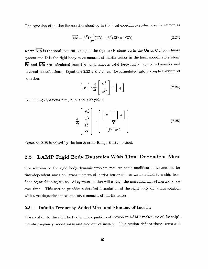
The equation of motion for rotation about cg in the local coordinate system can be written as
-~--d II __ -T-- -Mo = I I/-(w/) + L (V/ x Y/w/) (2.23)
where Mo is the total moment acting on the rigid body about cg in the Og or Og' coordinate
system and 1/ is the rigid body mass moment of inertia tensor in the local coordinate system.
Fo and Mo are calculated from the instantaneous total force including hydrodynamics and
external contributions. Equations 2.22 and 2.23 can be formulated into a coupled system of
equations
E - - = q (2.24)
Combining equations 2.24, 2.16, and 2.20 yields
d [E71[q] -
- -+ (2.25)
-+ [W] -4/
Equation 2.25 is solved by the fourth order Runge-Kutta method.
2.3 LAMP Rigid Body Dynamics With Time-Dependent Mass
The solution to the rigid body dynamic problem requires some modification to account for
time-dependent mass and mass moment of inertia tensor due to water added to a ship from
flooding or shipping water. Also, water motion will change the mass moment of inertia tensor
over time. This section provides a detailed formulation of the rigid body dynamics solution
with time-dependent mass and mass moment of inertia tensor.
2.3.1 Infinite Frequency Added Mass and Moment of Inertia
The solution to the rigid body dynamic equations of motion in LAMP makes use of the ship's
infinite frequency added mass and moment of inertia. This section defines these terms and
19

explains why they are used.4 -
LAMP calculates the total instantaneous force, Fo, and moment, Mo, for the ship rigid
body dynamic equations. Force and moment contributions from hydrostatics, the incident
wave, hydrodynamics, external forces, and body forces are used to calculate Fo and Mo. Due
to the total nature of the force and moment calculation the infinite frequency added mass and
moment of inertia for the ship are not required in the dynamic equations. However, they are
used in the LAMP rigid body dynamic solution for numerical stability.
The added mass and added moment of inertia terms are referred to the global coordinate
system when calculated. This causes them to be time-varying as the rigid body orientation
changes with respect to the global system. The added mass and added moment of inertia terms
are defined at an each time instant as
aij = p ji-dS i, j = 1, 2,..., 6 (2.26)// O#B
where a = ni, i = 1, 2,3 and L= (an x n)i-3, i = 4, 5,6. Vector . is the position vector
on the body, B, in the local coordinate system and - the outward normal of the fluid on B.
The global added mass matrix, Ao, is a 6x6 matrix constructed with term i, j of Ao equal to
aij. The terms in Ao are defined as 3x3 submatrices
Ao Al A12 0 (2.27)A 2 10 A220
2.3.2 Translation:
By replacing the rigid body mass matrix, Mo, with Mo + Am(t), the equation of motion for
translation can be written as,
Fo = -((Mo + Am(t))(V, - Uship)) (2.28)dt
20

For stability in the Runge-Kutta numerical integration scheme, added mass terms are added to
both sides of equation 2.28 to obtain
- A ( - - U d dFo+Ano (Vo) +A20() =-((Mo +Am(t))(Vo -AUship))+Ao-(Vo) +A 12 0 -( w)
(2.29)-4 -4 +
Rewrite equation 2.29 by substituting F for the left hand side where F Fo A1 1 o(V) +
A12A1 2 ot( w)
d - -+ 71-> dF = ((Mo + -Em(t)) (Vo - Uship)) + A-o- (VO) + 0 A - (W (2.30)
then group terms and carry out differentiation to get the final form of the translation equation
of motion
-+ - d -Tr d ->dF = (Mo + Am(t) + Ano)-(Vo) + A1 2oL T('/) + (Vo - Uship)-(Am(t)) (2.31)
2.3.3 Rotation:
The rotation equation of motion is expressed in the local frame O/. The local frame is used so
that derivatives of I and T do not have to be calculated.
Definitions and relations:
Some terms need definition prior to developing the rotation equation of motion. I is the rigid-- 4
body mass moment of inertia tensor in the Og or Og/ frame. H is the angular momentum
about cg in the Og or Og/ frame. H/ is the angular momentum about cg in the 0/ frame.
The following equations relate the rotational terms:
-- 4
H = (2.32)
/ =/Y/ (2.33)
Mo/ = TMo (2.34)
I=TTTIIT (2.35)
21

Formulation:
The equation of motion for rotation about cg in the 0/ coordinate system can be written as,
d -+4Mo/ = -(H/) (2.36)
dt
In order to expand the term d (H /),the following equation, which is a standard result from any
dynamics textbook for vector derivatives in rotating systems, is used,
(A )= (A w) x A (2.37)d d-+
In equation 2.37, A(A) is the absolute rate of change of A written terms of the unit vectors
in the rotating system, A (A)r is the rate of change of A as viewed from the rotating system,
and V is the absolute angular velocity of the rotating system. Placing the angular momentum
vector H/ into equation 2.37 gives,
d I d -+38-(H/) = -(HI/), f/ x4' (2.38)dt dt
The angular momentum as viewed from the rotating (local) system is,
(H-4/)r = 1/,/ (2.39)
inserting equations 2.33, 2.36, and 2.39 into 2.38 gives,
Mo/ = -(If/J/) + 'W/ x i/W/) (2.40)dt
Due to time varying mass, the rigid body mass moment of inertia tensor,I/, is replaced by
lo/ + AD/(t). Applying equation 2.34 to 2.40 and making the substitution for the time varying
inertia results in
LMo = - ((Io/ + AI/(t))D/) W/ x (o /+ AI/(t))L/) (2.41)dt
22

Then, by performing differentiation and moving L to the right hand side equation 2.41 becomes
Mo = W (o/+ AT/(t)) i/+ (AI/(t))U/ U/ x [(o+ AI/(t)) W/] (2.42)
Similar to equation 2.29, for stability of the numerical scheme, added mass terms are added to
both sides of the equation 2.42. Also, the substitution of M = Mo + A2 10o(V0 ) A 22 OA(Q)
is made so that
= ( o/+ AI/(t)) -/ + ( kL/())O/+ W/ x [o/ /())W/ + 210 VO) 220 ()
(2.43)
Finally, grouping terms gives the final form of the rotation equation of motion
M= A2 o (V [A 22 0LT + r (Io/+ A/)(t)))] )/l+rd -T(./x [(To/ + AI/(t))W-/)
(2.44)
2.3.4 Coupled Rotation and Translation Equations:
The translational and rotational equations of motion, equations 2.31 and 2.44, are a coupled
system
E - - = q (2.45)dt y
where
IAno+ Mo + Am(t) A122L.E ] _= (2.46)
A 2 10 A 22 OLT + LT(o + AII(t))
and
[ ~ ~F (Vo - Us hip) (Em~t)(.[- ] (/ x (lo/ + AI/(t))J/i)) - u (Al/(t)) ]The details of [E], and [q] were not shown in equation 2.24. They contain terms similar to
equation 2.45 except that there are some new terms in equation 2.45 due to the time-dependent
mass and mass moment of inertia. The new terms are (VO -Uship) T(Am(t)) in the translation
equation and T-i/A (A!/(t)) in the rotation equation. Also, mass and mass moment of inertia
vary with time in equation 2.45 but are constant in 2.24.
23

Chapter 3
Models for Flooding
3.1 Compartmentation
Watertight internal subdivision using bulkheads to form compartments within a ship has been
the primary means of limiting the extent of flooding in a damaged ship. During ship design,
various bulkhead arrangements are evaluated against operational and damaged stability re-
quirements to determine an optimal ship subdivision. In general, improved damaged stability
performance with increased subdivision must be balanced against drawbacks to compartmen-
tation such as weight, interference with arrangements, and access to systems.
The capability to compartmentalize hull geometry had to be added to LAMP in order to
model flooding for damaged stability analysis. Since this thesis is concerned with the basic
changes necessary to LAMP for it to be used as a damaged stability prediction tool, it was
considered adequate that the compartmentation model only use transverse bulkheads. If
required for a specific ship configuration or damaged scenario, more detailed compartmentation
model with longitudinal bulkheads and damage control decks could be added.
A LAMP program module was written to accept arbitrary transverse bulkhead locations
as input. The bulkhead locations are specified by their distance from the ship bow. The
distance is normalized through dividing by the overall hull length. Any number of bulkheads
can be created. The bulkhead locations are then automatically spliced into the hull geometry
description to form compartments that are bounded by forward and aft bulkheads, the hull, and
the weatherdeck. Compartments at the bow or stem of the ship use the hull geometry to serve
24

the place of a forward or aft bulkhead as applicable. Figure 3-1 illustrates compartmentation
of the bow of a DDG51 Class hull. In this figure the intersection of each line with other lines
Figure 3-1: Compartmentation Model of a DDG51 Class Bow
is described by an three dimensional coordinate point.
Consistency between the flooded volume calculation and the LAMP hydrostatic calculation
is important for an accurate representation of the ship's mean body position. Because the
compartmentation module uses the detailed LAMP hull geometry description to define the
majority of a compartment, the model provides excellent consistency between the compartment
flooded volume calculation and the hydrostatic calculation. Results were obtained for a ship's
final hydrostatic position after a flooding event. A comparison of the flooded volume against
the resulting change in ship displaced volume showed the two agreed to within 99%.
Finally, the compartmentation module is only used for calculations on the internal flooded
water and does not affect the hull geometry description. This is important because the hull
geometry description defines the body on which the hydrodynamic calculations are performed.
25

3.2 Calculations For a Compartment's Flooded Volume
For sloshing of a flooded volume of water it was conservatively assumed the water within a
rolling compartment maintains a horizontal surface. In actual ship compartments there are
generally some solid objects that will project through the surface of the water to reduce free
surface motion. Ship designers account for this effect through the surface-permeability factor.
The horizontal surface assumption produces a first order approximation for sloshing. For
simplicity, pitch motion was not considered in the flooded water sloshing calculations. Damaged
stability criteria mainly look at transverse stability while in a damaged condition and sloshing
due to pitch would have little-to-no effect on this stability. Ignoring pitch motion also made it
easier to check the accuracy of the flooded volume calculations.
Numerical solution techniques for calculating the instantaneous dynamic free surface in a
flooded compartment are an alternative to assuming a horizontal surface but they provide a
relatively small increase in accuracy compared to the significant increase in complexity and
calculation time. An actual ship compartment is outfitted and filed with equipment so even if
the instantaneous free surface were calculated it probably would not reflect the actual conditions
in the flooded compartment. Efforts to accurately calculate a free surface are better suited for
the shallow water flow problem that arises when shipping water.
Figure 3-2 illustrates the instantaneous position of a flooded compartment volume with the
ship undergoing a roll to starboard with roll angle, <Dr. The roll is made through the ship's
center of gravity, cg. The unprimed coordinate system in the figure, the YZ system, is the
LAMP initial static system which is used as the reference to describe the hull and compartment
geometry through position vector Rxyz. The primed coordinate system has been introduced
for the flooded volume calculation and rotates to maintain the Y/ axis parallel with the water
surface.
Flooded compartment volume is calculated in the YIZI system by summing the rectangular
parallelepipeds of length dely/ and height dzl. These are indicated in figure 3-2 and have a depth
dx along the hull's longitudinal axis. The parallelepiped geometry was selected to simplify
moment of inertia calculation. The flooded volume calculation is initiated by converting the
compartment geometry,R, to the primed coordinate system, R1, where C is the rotation matrix
26

Z
Y
<br-+ Y'
RxyzRgrav
CG w1
dely'
dz'
Figure 3-2: Compartment Flooded Volume Model
between YZ and YIZI,
RI= Rz Rgrav) (3.1)
Since only roll motion is considered, the x and x/ values are the same. If it were desired to
include pitch motion in the sloshing model, the pitch angle could be included in ~C and the
calculation proceed in the same manner as described here. The summation for volume is made
over x using j = Jmax intervals and over z/ with k = kmax intervals where x spans the flooded
compartment length and z/ ranges from the minimum value to the waterline wl
Vcmpt = ( ( dely/dz/dx (3.2)Xj Zik
At a fixed roll angle, the waterline value wl serves to determine compartment flooded volume.
If a specific instantaneous flooded volume is desired for a particular flooding scenario, wl can
be adjusted through an iteration process until the desired volume is reached.
The center of mass of a flooded compartment, CGcmpt = (X11, i 2 , i/ 3 ), can be calculated
where
/;i = xeii 1, 2,3 (3.3)
Equation 3.1 is then used to refer CGcmpt to the YZ coordinate system. With the flooded
27

volume and center of mass known, forces, moments, and the time-dependent mass terms can
be calculated due to the flooded water and added to the dynamic equations of motion 2.45. If
the flood rate is specified it is used directly as the ((Am(t)) term in the equations of motion.
Otherwise A (Am(t)) needs to be calculated based on the flooded volume time history.
The calculation for flooded water mass moment of inertia is made by summing the mass
moment of inertia of each parallelepiped about the flooded volume center of mass. Appendix
A outlines the method for doing this. After calculating the flooded volume mass moment of
inertia tensor about the center of mass, SMIcmpt, the parallel axis theorem and a rotational
transformation must be applied to refer SMcmpt to the ship's cg in the local coordinate system.
The instantaneous flooded volume mass moment of inertia tensor is used for the AI/(t) term
in the dynamic equations of motion. The (AI/(t)) term must be calculated based on the
flooded volume mass moment of inertia time history.
To better model an actual ship, compartment permeability could be used in the calculations
for a compartment's flooded volume. It would be a trivial matter to add permeability to the
calculations above.
3.3 Flooding Simulation
With the compartment flooded volume model established there are several approaches to run-
ning a time domain flooding simulation. First, the simulation can start with the initial condition
that the flooding event is complete and the ship is in its final flooded static condition. A com-
puter module was written to run this type of simulation. The module solves for a ship's final
static position after a flooding event in any specified compartments is complete. The module
uses an iterative procedure to calculate the final ship position and then revises the ship mass,
moment of inertia tensor, and cg location to account for the added water. Alternatively, the
module can maintain the ship intact and provide the total water that would be added if specific
compartments were flooded. This information can be used as an upper bound on flooded
compartment volume if it is desired to flood the ship as time advances in the simulation.
The second approach for a time domain flooding simulation is to start with either an intact
condition or some fully flooded compartments and then flood additional compartments as the
28

simulation time progresses. This approach is what is referred to as progressive flooding in
Chapter 1. The mass addition rate from flooding would need to be specified in this type of
simulation. One technique to specify this rate is to specify a hull opening location due to
damage and let water enter the compartment when the instantaneous free surface is above the
hole. The flow through the hole of area A and at static head h would be governed by the
short tube orifice equation, Q = CdA/2~g?. Tables may be obtained for the coefficient Cd from
textbooks on hydraulics such as LeConte [18]. In [6] Dillingham states Cd may be taken as
0.60 with very good accuracy.
3.4 Wind
LAMP is configured to include external forces in its calculation and currently has modules
that calculate external forces for items such as appendages, viscous roll damping, and moving
weights. It is a simple matter to include a heeling moment caused by beam winds using an
equation such as the following from reference [17]
M = K(Vw) 2Al(cos(<D,))2 (3.4)A
In equation 3.4 Vw is the wind velocity, A is the ship sail area, 1 is level arm from centroid of sail
area to half draft, 4r is the roll angle, and A is the ship displacement. K is a constant whose
value can vary depending on units used in the equation and on assumptions on values for wind
drag coefficient. Reference [17] contains a discussion on calculating wind heeling moments.
Equation 3.4 could be expanded to include the wind heading angle so that three dimensional
wind forces and moments on the ship are included in the LAMP calculation.
3.5 Causes of Loss of Accuracy in LAMP Flooding Simulations
When linear hydrodynamics are used in LAMP to solve the potential flow problem (LAMP-I and
LAMP-2) the initial mean body boundary position is used for the duration of the calculation.
However, due to sinkage and trim from flooding the actual mean body boundary position will
change. As the flooding ship's mean body position diverges from the initial position a loss of
29

accuracy in the calculated ship motions will result.
One strategy to limit the loss of accuracy in a flooding simulation using linear hydrodynamics
is to select an intermediate body position between the intact and final flooded conditions.
Another approach would be to run the linear hydrodynamics LAMP simulation at the intact
body position and then at the final flooded body position and use the worse case ship motions
as the motion estimate. Of course, non-linear hydrodynamics (LAMP-4) could be used for
the flooding simulation but the penalty is that much more time is required to perform the
calculation.
As water floods into the ship it causes a time-dependent shift in the ship's center of gravity,
cg. This shift is not accounted for in the LAMP dynamic equations of motion solution. For a
small amount of flooding in a massive ship the shift in cg will be trivial. Under these conditions
the calculated ship motions would be reasonably accurate. However, as the magnitude of the
cg shift increases, the calculated angular ship motions will be wrong because the rigid body
moment determined at each time step grows in error.
Finally, when simulating significant hull damage such as a compartment size hole, consid-
eration should be given as to whether complete body panelization that assumes an intact hull
will provide an accurate enough hydrodynamic solution. A more accurate method may be to
re-panelize the hull around the physical damage.
30

Chapter 4
Models for the Green Water
Problem
4.1 Background and Scope of Green Water Model
As a flooding ship loses freeboard, the likelihood of shipping water increases. The water on
deck, in turn, can further degrade the ships stability condition. This is of special concern for
smaller vessels. A review paper on the subject of water on deck and stability of has been
published in reference [3]. Also, in reference [6], Dillingham provides calculations to show that
instabilities caused by excessive deck water may cause capsizing of small fishing vessels. The
green water problem can be decomposed into three subproblems: shipping water, water escaping
off deck, and the motion of water on deck. For adequate modeling of the green water problem
in a time domain ship motion program each subproblem must be addressed.
Most work reported on the green water problem has focused on the water motion on deck
subproblem. This emphasis over the other two subproblems is primarily due to water-motion-
on-deck sharing the same basic theory as that for flow of compressible gases. Specifically,
the equations governing water motion on deck, equation 4.13, are derived from the theory for
waves in shallow water, covered in detail in reference [29], and are of the same form as the
compressible gas dynamics equations. The necessity in industry for dealing with the flow of
gases has resulted in numerical solution methods that can be directly applied to the water-
motion-on-deck problem. The objective in solving the shallow water equations is to solve for
31

the water depth and horizontal particle velocity. Solutions to the governing equations can
involve discontinuities such as shocks, bores, and hydraulic jumps. Any numerical methods
used to solve the equations must be capable of treating discontinuities. Most of the numerical
methods fall into two general categories characterized by the scheme used to solve the governing
equations: the flux difference splitting method and the random choice method, also known as
Glimms Method. Both schemes handle discontinuities in the solution without any special
treatment and were evaluated in this thesis. The Random Choice method involves looking
at solution curves, called characteristics, to the governing differential equations. The flux
difference splitting method combines a finite difference method with characteristics. A different
approach to solving the water on deck problem is in reference [13] where the authors solve for
wave motion in a rolling tank using a finite difference scheme coupled with analytical techniques.
This approach illustrates the special care that must be taken with discontinuities with which
the numerical scheme is incapable of handling.
This chapter develops a green water model for the LAMP program in head seas. The two
main methods for solving the water-on-deck subproblem are evaluated for use in the model using
a two-dimensional free surface. A method for incorporating water shipping into LAMP is also
devised. The water escaping off deck subproblem is not formulated because a proper calculation
would require a three-dimensional free surface solution to the shallow-water problem. Three
dimensions would introduce transverse water velocities so that as the green water travels aft on
the weatherdeck it also moves towards the port and starboard deck edges and then over board.
The green water model used for this thesis only calculates longitudinal water velocities so green
water mass is removed from the weatherdeck by letting it fall off the after end of the portion
of the weather deck included in the computation. This is accomplished by setting boundary
conditions for the water-on-deck calculation to zero at the aft end of the weatherdeck
4.2 Flux Difference Splitting Method for Water Motion on Deck
The flux difference splitting method was developed based on the flux vector splitting method
originally introduced by Steger and Warming in [28]. Steger and Warming developed a basic
theory of the flux vector splitting method to compute the shock wave for the gas dynamic equa-
32

tions. Because of differences between the non-homogeneous governing equations for shallow
water flow on deck and gas dynamics, it is better when solving the shallow water equations
to split flux differences instead of the flux vector. In reference [1] Alcrudo presents the flux
difference splitting method to solve problems for open channel hydraulics. In references [12]
and [11] the flux difference splitting method is applied to solve the shallow water flow on deck
problem.
The flux difference splitting method is a an upwind (one-sided) finite difference scheme that
solves the shallow water wave propagation problem for a two dimensional free surface. For
supercritical flow, wave information can only travel downstream. In the case of subcritical
flow, wave information will travel in both directions. In order to construct an upwind scheme
valid for all regimes and directions of flow, a decomposition of the flux related to positive
and negative propagation speeds is needed. The flux decomposition is devised so that wave
information can not travel upstream in supercritical flow. For flux difference splitting methods
the flux difference operator, A F and ARHS in the equations below, is split based on the
characteristic directions.
Reference [12] can be used to formulate the shallow water flow governing equations for a
two-dimensional free surface with the geometry illustrated in Figure 4-1. Many of the variables
in the governing equations are not defined in the figure. Of these, ui is the ship surge velocity,
u3 is the ship heave velocity, E is the pitch angle, u5 is the angular velocity, and g is acceleration
due to gravity. Note that u is the water particle velocity in the x-direction. The governing
equations in vector form is
aW a F O H -+ = [D] + C (4.1)
go _,Ug( 0 0 0whereW= ,, F= ugH ,g) 2 [D](= qjg(+q2U+q3
ug u2g+(gC)2 2
and C = . The variables qi through q4 are functions of deck motion and geometry.
(q4g(They are defined as
U5 2qj (9)
33

z
ZG
CG
Figure 4-1: Coordinate System for Two-Dimensional Free Surface
U5q2= 2-
9du3 1
q3 = cos(9)dt g
du5 Xdt g
(u5 )2 ZG
g
fdull\ dU5Zq4 = sin()- d + U + du ZG
Equation 4.1 is derived by applying the shallow water assumptions to the continuity equation
and Eulers equations of motion.
The derivatives of the flux vector F and H can be expressed in terms of W
a F49X
4W=[ w
o71and
(9X
-4
= [J2 ] Ox(4.2)
where [J1 ] and [J2 ] are the Jacobian matrices. The eigenvalues of [Ji] are
A = u + V/g9 and A 2= U - V
with the eigenvectors
el= (1,u+ V) and e=
34
(4.3)
(4.4)

The difference of W and flux vector F are approximated as
2
AW4= Zak ekk=1
2
and AF = S Akakekk=1
The right hand side of equation 4.1 equal to zero corresponds to water sloshing for a given
initial water surface profile and the ship stationary. With the right hand side zero, the finite
difference scheme with the split flux difference can be expressed in the following form
( n + _ )(- (A tW W + F* F*(4.6) i AX 3--f i+7
where1 -4 -4 1 2
F* = -(F j+1 + F ) 2 ak,j+i -1 AkJ+i ekJ+3 2 k=1 2 22
2-
2 k- -4
F( F +Fk1) - 2ak A e2 k=1
(4.7)
(4.8)
The scheme in equation 4.6 is of the first order.
When the right hand side of equation 4.1 is not equal to zero,
difference term and projected into the eigenvector space as follows
-+ 2RH(= [D H 1
The right hand side flux difference, where the flux difference is
ARHS = RHSAx, is then split
)+ 2 2
ARHS.t %J-L+ and ARHS = EAH 2=- k1
k=12k=
it is treated as another flux
r( t4.9)
related to equation 4.9 by
Yk,J+ kj ekJ+ e
where
A Z1- = (AkJ.1 AkJ--I) and A i+ . (A J 1 Ak~jk, T1 , 1
The split flux difference is then included in the finite difference scheme of equation 4.6
W(n+l) - (n) At ( A H + )A x J ~ i2 x i T 1 A+ 7h~
35
(4.10)
(4.11)
(4.12)
(4.5)

The minus sign in equation 4.12 prior to the RH term is due to the minus sign in equation
4.9. In [28] Steger shows that flux splitting schemes are stable if and only if A - < 1.
Shallow water first-order schemes suffer from numerical dissipation (the shock front will be
smeared). Reference [12] shows how a flux limiter, which is a correction term for the numerical
flux, can be applied to the first order scheme to make the scheme higher order.
The flux difference splitting method can be used to solve the shallow water equations for a
three-dimensional free surface. Reference [12] formulates a technique using the flux difference
splitting method, together with the Fractional Step Method [32], so that solutions to the shallow
water equations can be obtained by solving two sets of two-dimensional free surface problems.
The three-dimensional solution works as follows. Two sets of vector equations similar to
equation 4.1 are devised. One set is for flow in the ship longitudinal direction (x - axis)
where each specific equation holds for a certain deck strip of thickness Ay. The other set of
vector equations is for flow in the transverse direction ( y - axis) where each equation is for a
certain deck strip of thickness Ax. Then the Fractional Step Method advances the solution in
time. At each time step the sets of equations along the x - axis are solved for an intermediate
solution assuming no y dependency. Then, in the same time step, the sets of equations along
the y - axis are solved from the intermediate solution assuming no x dependency. Instead
of solving the three-dimensional free surface governing equation on (m x n) nodes, a total of
(m+n) two-dimensional free surface equations are solved along the x and y directions separately
using the Fractional Step Method.
The difference schemes of equations 4.6 and 4.12 for a two-dimensional free surface were
programmed in a computer so that the method could be compared with Glimms method.
4.3 Glimms Method (Random Choice Method) for Water Mo-
tion on Deck
For a two-dimensional free surface, Glimms Method is performed by dividing the physical
domain into intervals, i = 1, 2, 3, ... , i max. In each interval at time nAt the solution is approxi-
mated by piecewise constant depth, (j, and particle velocity, ui. At the boundary between each
interval, the depth and velocity are therefore discontinuous which gives a sequence of Riemann
36

problems which may be solved to advance the solution to time (n + 1)At. The solution to
the Riemann problem is outlined below and the full solution is developed in Appendix B. The
Riemann problem is also known as the dam breaking problem. From the time (n + 1)At Rie-
mann solutions, it is desired to construct another piecewise solution. This is done by randomly
sampling the solution in each interval and then using the sampled value as an approximation for
that interval's constant piecewise solution. In [10] Glimm showed the random sampling scheme
converges to a weak solution. The disturbance resulting from the solution for each individual
Riemann Problem must not be able overlap with the disturbance from the adjacent Riemann
Problem. No disturbance must be allowed to propagate further than Aintervl in a time At.
Thus the resulting Courant condition that must be satisfied is Ainterval + V ). The
solution obtained is unconditionally stable.
Glimms Method is used to solve the water motion on deck problem in references [6], [22],
and [23]. References [27] and [4] illustrate use of the Glimms Method to solve gas dynamic
problems.
Appendix C contains a MATLAB program that solves a Riemann Problem using Glimms
Method.
4.3.1 Solution of the Riemann Problem
Glimms method requires solution of the Riemann Problem, also known as the dam breaking
problem, at each spatial interval in the computational domain at each time interval. A summary
of the Riemann Problem solution procedure, taken from Dillingham [6] follows. Appendix B
provides details of the calculations. In keeping with Dillingham's notation, the y axis is used
as the coordinate axis for the Riemann Problem, v is the horizontal velocity, and A is used for
the water depth.
The Riemann Problem, illustrated in figure 4-2, consists of solving a system of nonlinear
hyperbolic equations, called the shallow water wave equations,
v av c9A iA DA 9v-+V- + -=V0 and -+v-+A--0 (4.13)
n f s w a eti sb y i
for a two-dimensional free surface where g is gravity acceleration, subject to initial conditions
37

on the right-hand and left-hand sides
V = V2 y < 0 andV = V y> 0A =y>o
I Initial DamI Position
22 V2
y=o
(4.14)
Figure 4-2: Initial Conditions for the Riemann Problem
It is assumed that the water is initially higher on the left side of the dam. The dam is then
removed at time t = 0. Depending on initial conditions, the Riemann problem solution falls into
different categories, identified as Cases I through V. The variable c as used below represents the
wave propagation speed; it is the local speed of propagation of "small disturbances" relative
to the moving stream. In shallow water theory, c is related to the water height by c = V/g~A.
Solution to the Riemann Problem: Case I
If V2 + 2c 2 > Vo + 2co and
V2 - 0 < g (Ao + A,)(Al - Ao)21 2 (4.15)12 A1Ao
then the solution consists of a single shock and a single rarefaction as indicated in figure 4-3Let
co = / A, ci = 'iM,and c2 = A Also, let R = 0 where is the shock speed, then
38

Figure 4-3: Solution for Riemann Problem Case I
solve the following equation for R
I
/8 R2 + '12/V2 - Vo + 2c 2
Co
then we have
S= coR +Vo
Vi = co R - (1+ 8R2+1)] +Vo
Ci= co (v/8R2 + I - 1) and A =g
In zone 3 we have
- V+V2 VO + c2) +Vo and A= (V29g \
where zone 3 is bounded by (V2 - c2) t < y < (V1 - c1) t.
Solution to the Riemann Problem: Case II
If equation 4.15 is not satisfied then the solution consists of two shocks as indicated in figure
4-4
39
V2
)\2 V3 yI VoK3 IM\ ?AO
(4.16)
(4.17)
(4.18)
(4.19)
V= (3 \.t
+ 2c 2 - (4.20)
R - - [1 + N/8-R2+ 1] + 24R

Figure 4-4: Solution for Riemann Problem Case II
Solve the following equation for A,
V2 -vo-g (Ao + A)(A1 - Ao)2]V2 V -2 A1Ao
A1 1 - AOV0
g (A1 + A 2)(A 2 - AI)2
2 A2 A 1 _
A2V2 - A1V1and '2 =
Solution to the Riemann Problem: Case III
If V - V2 > 2 Ico - c21 then the solution consists of two rarefaction waves as in figure 4-5The
solution for zone 1 is
V = 2 + C2 - co and Al =g + 2(4.24)
In zone 3 we have
and A = (V2 + 2c 2 - 2 (4.25)
40
then
2
= 0 (4.21)
(4.22)
(4.23)
V2 V1 1 6A2 A
Vo
2
(y + C2V + L
3 t 2
V VO + [g (Ao + A1)(A1 - Ao)2 2
2 A1Ao

V2
V3 VI V4 Vo
X\3 X4
Figure 4-5: Solution for Riemann Problem Case III
where zone 3 is bounded by (V2 - c2 ) t < y < (V1 - c1 ) t.
+ V2
In Zone 4
and A = I 2 co -Vo+ )
where zone 4 is bounded by (V1 + c1) t < y < (Vo + co) t.
Solution to the Riemann Problem: Case IV
If AO = 0 then the solution is a single rarefaction wave as in figure 4-6.
V2
V3X\3
Figure 4-6: Solution for Riemann Problem Case IV
The solution in Zone 3 is
= + + and A= 2c 2 +V 2
41
(4.26)
(4.27)
v = 2(

where zone 3 is bounded by (V2 - c2) t < y < (V2 + 2c2) t.
Solution to the Riemann Problem: Case V
If in case III there is the additional condition that V2 + 2c 2 < V - 2cO then the water depth
will be equal to zero in Zone 1 and the problem must be treated similarly to Case IV.
4.4 Selection of Water Motion on Deck Method
Computer programs for the flux difference splitting method and for Glimms method were gen-
erated to solve a Riemann problem. The goal of this effort was to compare the methods to
see which is most suitable for incorporation into the LAMP water on deck model. Figure 4-7
illustrates the solution to a Riemann problem using a first order flux difference splitting method
scheme without flux limiters. The solid line is the exact solution, the other two lines are the
numerical solutions. The line with the shorter dashes is for - = 0.005 and the line with the
longer dashes is for -A = -t oo0. The scheme converges to the exact solution as Ay is madeAy 0.01
smaller.
Figure 4-7: Riemann Problem Solution Using Flux Difference Splitting Method
Figure 4-8 illustrates the solution to the same Riemann problem using the Random choice
method. The solid line is the exact solution, the other two lines are the numerical solutions.
42
0.65
0.6
0.55
0.5
0.45
0.4
0.35
0.3
0.25
\j.0.5-0.5 -0.4 -0.3 -0.2 -0.1 0 0.1 0.2 0.3 0.4

The line with the shorter dashes is for ' = 02 and the line with the longer dashes is for
t 0.001. This scheme also converges to the exact solution as Ay is decreased.AY 0.01
Due to the random interval sampling required in this procedure, the results vary each time
the calculation is run. For example, for constant At, Ay, and initial conditions, a set of
calculations will produce a unique solution curve for each calculation. Figure 4-9 shows three
different solutions to a Riemann problem, the dashed lines, using the Random Choice Method.
For each solution the initial conditions and calculation parameters were the same.
Other Riemann problems were investigated to compare the Random Choice and first order
flux difference splitting methods. Table 4.1 summarizes a comparison of the two methods.
An "X" entered in the Table means that method is superior to the other method in the given
category.
Comparison Category Random Choice Method Flux Splitting Method
Ease of Programming X
Accuracy for Given Discretization X
Repeatability of Solution X
Ability to Capture Discontinuities XTable 4.1: Comparison of Shallow Water Solution Methods
The flux difference splitting method was selected, primarily due to ease of programming, as
the numerical method to be used for the for LAMP green water model.
4.5 Water Shipping Model
The difficulties in creating a realistic water shipping model are best framed by Dillingham in
[6]. He states, 'In general the flow over the bulwark is very complicated since it results from
the unsteady interaction between shallow water waves on the deck and deep water waves off
the deck. In addition, direct observations of models indicate that the deck water may regularly
impinge on the bulwark with considerable velocity and be thrown over the side in what amounts
to a spray. To refer to this process as either turbulent or nonlinear is an understatement."
For water shipping to occur, the height of the free surface at the ship side must exceed the
height of the bulwark (or deck edge if there is no bulwark) and the relative velocity of the water
above the top of the deck edge must be directed inward onto the deck. The height of the free
43

0.65,
0.6
0.35
0.3
0.25 Ix0.2L
-0. -0.4 -0.3 -0.2 -0.1 0 0.1 0.2 0.3 0.4 0.5
Figure 4-8: Riemann Problem Solution Using Random Choice Method
0.65
0.6
0.55 -
0.5-
0.45 -
0.4
0.35
0.3
0.25 -
0.2 -- --
-0.5 -0.4 -0.3 -0.2 -0.1 0 0.1 0.2 0.3 0.4 0.5
Figure 4-9: Solution Randoness in Random Choice Method
44
0.55
0.5
0.45
0.4
5

surface above the bulwark or deck edge is referred to as the relative elevation, rIR. This thesis
makes use of a ship model with no bulwark so hereafter only the deck edge will be mentioned
in the water shipping discussion. Figure 4-10 illustrates some geometries and variables used
in the water shipping model. The XZ coordinate system represents the global system which
maintains a fixed orientation. The primed system, XIZI, is the local coordinate system that
moves with the ship. The variable q represents the free surface elevation and Zd represents the
height of the deck edge. Each is referred to the global system as a value along the z axis. The
instantaneous relative elevation would be 17R(t) = 7(t) - Zd(t). The vectors V ,, and V W,
are components of the water particle velocity V,,. The vectors V d, and Vd, are components
of the deck edge velocity Vd. All vectors are referred to the global system.
Vwy
JL~w Freez d y Idx 7 Surface
Zdxpitch ----- ----------
CG X angle
Figure 4-10: Geometry and Variables for the Water Shipping Model
4.5.1 Free Surface Elevation for Water Shipping
A basic description of the instantaneous free surface, q(t), can be made by considering only the
incident wave potential. However, for a more accurate description of the free surface around the
ship hull the complete incident, diffracted, forward speed, and radiated wave system potentials
should be used. The hydrodynamic potentials cause an increase in free surface elevation which
45

is commonly referred to as "pile-up" in the wave-body interaction. For a more complete
estimation of pile-up the jet motion of the free surface from water-entry and slamming should
be considered. In reference [8] a numerical technique for predicting the occurrence of water
shipping is presented and it is concluded that the radiation and diffraction terms play important
roles in the water shipping analysis and cannot be neglected.
For the water shipping model presented here, the incident wave potential is used for calcu-
lating the free surface height at the ship side. An elevation correction is then made to account
for the forward speed, radiation, and diffraction potentials. The hull surface hydrodynamic
pressure at the body panel adjacent to the waterline and nearest the desired deck location is
used to compute an elevation which is added to the relative elevation computed from the ship
motion and incident wave potential.
For a LAMP-2 calculation of the CG-47 hull in storm seas case, this elevation correction did
not prove to be particularly large most of the time. It is probable that the correction would
be larger for a LAMP-4 calculation, as the hydrodynamic calculation would include some hull
flare effects.
4.5.2 Relative Velocity for Water Shipping
Several terms must be considered to determine the relative velocity, V,, of the water above the
deck edge. The water particle velocity, V W, and ship velocity at the deck edge, V d, must be
known. Also, an additional velocity due to the effect of hydraulic flow, Vh, must be included.
Hydraulic flow occurs due to energy conservation from converting the static head from the
relative elevation into a velocity according to Bernoulli's equation. Referring to figure 4-11,
where the variable z/ is the local height off the weatherdeck, the static head height is (7 - Zd) -z/
and the hydraulic velocity is Vh(z/) = 2g(jg -7z/). The hydraulic velocity is assumed to be
directed onto the ship parallel with the xf axis. The dependency that Vh has on z/ can be
removed by averaging Vh over the static head. This is done with the following integral to
obtain mass flow rate, Q,
J7-Zd =2g(nR - z/)dz/ (4.28)
In [6] Dillingham uses a technique similar to equation 4.28 to integrate for the mass flow rate
onto a ship's weatherdeck. Carrying out the integration in 4.28 and then dividing by the static
46

head height to obtain an average hydraulic flow, Vhave gives
2Vhave -- -TgTR3
(4.29)
The water shipping model, then, uses Vha,,v,, , and V d for the relative velocity calculation.
The calculation for Vha., is a simplification made for this thesis. In reference [11] the
hydraulic flow contribution to water shipping is treated within a more general calculation for
mass of the wave shipped on deck. The mass calculation is performed by integrating around
the edge, L, of the weatherdeck as follows,
Mass = P VJf - Vd)dzI + Vh(zi jdzj dldt0 L 0 f0
(4.30)
The constant C, in equation 4.30 was determined experimentally by Grochowalski to be 0.55.
ZI
X'
Zd
77FreeSurface
Figure 4-11: Water Shipping
Because V,, and V d are vector quantities, the calculation for V, can be performed several
different ways depending on the assumptions made. These calculations will be referred to as
Methods I, II, and III. In any case, since shallow water theory assumes all fluid velocity is
parallel with the deck surface, the direction for V,, shown in figure 4-11, is always considered
to be parallel with the weatherdeck. For Method I, the calculation will use only the horizontal
47

components of the wave and particle velocities so that
Vr =Vdx - Vx + Vhave (4.31)
For Method II, the calculation will consider the ship's instantaneous pitch angle, e, and use
the components of the vectors V X, Vw,, V dx, and Vd, that are parallel with the V/ axis.
The calculation for V in this case is
Vr = Vx cos(@) - V, sin(E) - (Vwx cos(e) - V,, sin(E)) + Vhav (4.32)
The Method III calculation will be performed by conserving the momentum of the water particle.
For long crested head seas there are only two wave particle velocity components so that
Vr = Vd, cos() -V sin() i + + Vhave (4.33)
where the plus (+) is used when (Vwx cos(e) - Vw, sin(s)) < 0 and the minus (-) is used when
(Vwx cos(e) - Vw, sin(E3)) > 0.
The relative velocity and elevation must be calculated at each time step. As indicated in
figure 4-11, the velocity is considered to be a constant from the deck edge to the top of the free
surface. With the relative velocity and elevation of the water at the deck edge known, they
can be considered as boundary conditions for a water on deck problem. When the relative
elevation becomes negative, the boundary conditions are set to zero. Evolving the water-
on-deck problem through time, with the relative velocity and elevation boundary conditions
updated at each time step, will result in mass flow onto the deck. Water shipping, therefore,
is treated as a boundary condition to the water on deck problem.
4.6 Green Water Model in LAMP
To create a green water model in LAMP for head seas, a weatherdeck was included in the hull
geometry description. The deck was modeled as a surface projecting aft from the ship bow
a distance approximately 25% of the overall ship length. The weather deck is divided into
strips of width dely. At the center of each strip is a deck edge reference point at which data
48

needed for the water shipping problem is calculated. Figure 4-12 illustrates this setup. The
Figure 4-12: Weatherdeck Division for LAMP Green Water Model
model uses the flux difference splitting method to solve the shallow water problem in each strip
as a two-dimensional free surface. Transverse water flow (from one strip to another) is not
calculated.
A LAMP subroutine was provided by SAIC to calculate, at each time step, the deck edge
motion, deck edge location, free surface height, and incident wave particle velocity for each
reference point shown in figure 4-12. With this data, the relative elevation and velocity can be
determined for each deck edge point.
After solution of the shallow water problem for each strip at each time interval, the forces,
moments, and the time-dependent mass and mass moment of inertia terms in the dynamic
equations of motion can be calculated that result from the water on deck. Because of the time-
dependent mass terms in the dynamics equations of motion, the green water on deck is treated
as part of the rigid body. Thus the only green water induced forces and moments that need to
be calculated for rigid body motion are those due to gravity acceleration. For the local loads
on the weatherdeck and superstructure, however, the absolute green water fluid acceleration in
the local coordinate system must be calculated. Let aow be the absolute acceleration of the
49
dely
/\I X

green water in the local ship coordinate system. As defined previously V is the rigid body
velocity at cg and W the rigid body rotation. Then from simple dynamics
-_4
aG = d + - (r/ W x W /) +2 x V/+ e (4.34)dt dt
where 4/ and V/ is the position and velocity, respectively, of the green water referred to the
local coordinate system. The vector a 2 is the acceleration of a point in the green water
measured relative to the local frame by an observer attached to the local frame. This quantity
is zero for the green water problem. The vertical acceleration component of aG is defined as
a,/. At each time step a,/ can be calculated for the green water on deck as a function of the
x axis in figure 4-12. The total deck pressure, Pdeck, is then be calculated by including the
gravity static head, which must include pitch angle, and the depth of the green water, (, so
that
Pdeck =p (az + g cos(E)) (4.35)
Forces from green water on large superstructure, where the water particle velocity at the struc-
ture boundary can be approximated as zero over a wide area, can be calculated from equation
4.35 by integrating the pressure through the water column. For smaller weatherdeck structures
a better estimate of the local green water loads may be made by considering the green water
particle velocity.
Figure 4-13 visualizes a solution to the green water problem by plotting the water depth for
one strip over a series of time steps with a sinusoidal incident wave. In this case the ship is
moving to the right into the sea, the bow is on the right, and time is increasing with the higher
curves. The horizontal portion of each curve is an area where the deck is dry.
50

Figure 4-13: Flow Visualization of Green Water on Deck
51
4)
4)
CO
-20 -10Deck X-Axis Location (x=-O at Bow)

Chapter 5
Validation and Results
5.1 Validation
5.1.1 Validation of Dynamic Equation of Motion Solver
The changes to the LAMP dynamic equations of motion to include time-dependent mass and
moment of inertia were validated using the model shown in Figure 5-1. The model is a body
with two lumped masses, M,, at the ends of a massless rod. The body has initial linear velocity
Figure 5-1: Model Used to Validate Dynamic Equations of Motion Solver
V, and initial angular velocity w whose vector representation is pointed along the x axis. The
52
x Vo
Mo

solution for linear and angular velocity over time was calculated as the mass was reduced at a
constant rate. At time t = 0.5 the mass reduction was ceased. The results in figures 5-2 and
5-3 show linear momentum, P, and angular momentum, H, is conserved in the calculation.
In each figure, the horizontal line is the constant momentum and the slanted line is either the
mass (figure 5-2) or the moment of inertia (figure 5-3). The parabolic line is either the linear
velocity (figure 5-2) or the angular velocity (figure 5-3).
Figure 5-2: Conservation of Linear Momentum
5.1.2 Validation of Compartment Flooded Volume and Moment of Inertia
Calculation
The flooded compartment module added to LAMP calculates volume, mass center, and moment
of inertia. The module also calculates a final hydrostatic position after flooding is complete in
any number of specified compartments. These calculations were validated by running them with
a rectangular hull geometry input. Separate calculations were made with the same rectangular
hull using different calculation methods and software. Results from the LAMP module agreed
with results from the independent method to within 99%.
53
4.57
4 ~
E :. 3.5-
0
0.5-
0
Time

Figure 5-3: Conservation of Angular Momentum
5.1.3 Validation of Flux Difference Splitting Method
A bore propagation problem is solved to validate the flux difference splitting method used for
the water motion on deck problem. In particular, this problem validates the homogeneous
form of the difference scheme, equation 4.6. The initial conditions are a Riemann Problem
v = 0.2667y < 0
A = 10.8and
v = 1.6Y > 0
A = 1.8(5.1)
where the velocity units are m/s and the water height units are m. The exact solution to the
problem for water depth has been given by Stoker in [30]:
10.8
1 (20.84 - )2
4.716
1.8
for
for
for
for
y < -10.0t
- 10.Ot < y < 0.45t
0.45t < y < 10.7t
y > 10.7t
The exact solution shows that a bore travels in the positive y-direction with a velocity of 10.7
m/s, and a rarefaction wave propagates in the negative y-direction at a speed of 10.0 m/s.
54
4.5
4
E3.5
E0 3-
25-
>1.5
0.5
0 '0.25 0.5 0.751Time
A(y, t) =

Figure 5-4 shows the numerical results (dashed line) and the exact solution (solid line) for the
water depth. The numerical results match well with the exact solution. Because the numerical
scheme is first-order, it has some difficulty handling the shock front. This is evident in lost
resolution and that the shock front travels slightly faster than the exact speed. This can be
corrected with a higher order scheme.
11
10
9
8
7
6-
5-
4
3
2
-15 -10 -5 0 5 10 15
Figure 5-4: Bore Propagation at t = 0.5 seconds
A second problem was used to validate the flux difference splitting method when the ship is
undergoing motion. Mathematically this is the condition where the right hand side of equation
4.1 is non-zero. This problem, then, is a test on the numerical scheme used for equation 4.12.
The problem is one solved by Huang and Hsiung in [12] for sloshing inside a deck well. The
computations are carried out for the deck flow excited by roll motion. The deck is 1 meter
wide, oscillating about a pivot which is 0.522 meters above the deck, and the roll amplitude is
0.067 rad. The mean water depth is 6 cm. The primary resonant frequency of the shallow-
water motion inside the deck well is w, = 2.41 rad/ sec. The numerical results in figure 5-5
are for a rolling frequency of w = 0.9 rad/ sec, well below resonance, to show the water behaves
as a "horizontal surface." The rolling frequency was then increased to twice the resonance
frequency and results plotted in figure 5-6. At this frequency, standing waves are formed with
the wave length approximately equal to the deck width. In each figure, plots were made of the
55

free surface at several time instances to illustrate the motion.
Figure 5-5: Shallow Water Sloshing Below Resonant Frequency
5.2 Results for Flooding Models
This section provides some results from the compartment flooding model that was added to
LAMP. In all cases, unless noted otherwise, the LAMP-2 formulation was used. The results
include effects on roll and pitch motions from a flooded volume and examples of inaccuracies
that arise due to a shifting cg and due to a changing mean body boundary position when linear
hydrodynamics are used. The ship model that was run in LAMP for these results is a CG47
Class Cruiser. A steady forward speed of 10 knots was used for all the calculations. This ship
model was used on the recommendation of SAIC due to its excellent past performance.
All plots of ship motion were made in non-dimensional units. If the ship has length L then
linear motions are made non-dimensional by dividing by L and time is made non-dimensional
by dividing by J. Angular motions are plotted in radians.
56
0.14
0.13
0.12
0.11
0.1
0.01
-. 0.07
4y 0.0(
0.050.04-0.030.020.01
-0.25 0 0.25Y (M)

Figure 5-6: Shallow Water Sloshing, Twice Resonance Frequency
5.2.1 Roll Motion Results
The first results, figures 5-7 and 5-8, show the effect of flooding and sloshing on roll motion.
Beam seas with a single sinusoid wave component were used to induce ship roll motions. A
large amidships compartment with length equal to 20% of ship length was created for flooding.
The bulkhead locations were at 0.4 and 0.6. Figure 5-7 illustrates roll motion of the intact hull
(solid line) and of the flooded ship (dashed line). For the flooded ship, the problem was started
with the ship in its final flooded position from uncontrolled flooding into the compartment and
sloshing was not included in the calculation. The linear hydrodynamics and sinusoid seaway
cause the motion to reach steady state after the starting transients pass. The roll motions of
the flooded ship are much reduced compared to the intact ship due to the flooded mass having
lowered the ship's cg. Sloshing effects were then added to the calculation. Figure 5-8 compares
roll motion of the flooded ship without sloshing (solid line) and with sloshing (dashed line).
The sloshing causes a roll moment, the effects of which can clearly be seen in the increased roll
amplitude.
57
0.1
0.075
CL
0.05-
0.025 -
-0.25 0 0.25y (M)

5.2.2 Vertical Motion Results
The next set of results, figures 5-9 and 5-10, show the effect of flooding on vertical motion and
relative elevation at the bow. Head seas with a single sinusoid wave component were used
to induce pitch and heave motions. The wavelength was set at 1.5 times the ship length to
excite pitch motion. Wave amplitude was 17 feet to approximate about a sea state 6. These
extremely harsh conditions were intentional to create a large relative elevation at the bow for
water shipping. A forward compartment with bulkhead locations 0.1 and 0.25 was created for
flooding. Figure 5-9 illustrates pitch motion of the intact hull (solid line) and of the flooded
ship (dashed line). For the flooded ship, the problem was started with the ship in its final
flooded position from uncontrolled flooding into the compartment. The trim of the flooded
ship is indicated in the initial pitch angle. Sloshing was not included in any of the pitch
calculations. The effects from the longitudinal moment induced by the flooded water and its
moment of inertia can be seen in the flooded ship motions. Notice that the flooded ship spends
a greater amount of time than the intact ship with the bow pitched downwards (positive pitch
angle). In such a condition shipping water is more likely to occur which is why a green water
model is also necessary for LAMP to be used as a damage stability prediction tool. There
is little difference in the intact and flooded ship heave motions for the same flooding scenario.
Figure 5-10 illustrates this motion for the intact ship (solid line) and flooded ship (dashed line).
The motions are similar but the flooded ship's vertical position is offset due to its lower cg.
The relative height of the bow deck edge above the instantaneous free surface 1 is calculated
for water shipping and can be plotted for the pitch motions in figure 5-9 This relative bow
height is shown in figure 5-11 for the intact ship (solid line) and the flooded ship (dashed line).
Shipping water occurs during a negative relative bow height (positive relative elevation). The
time duration and magnitude of each shipping water event is greater for the flooded ship.
5.2.3 Loss of Accuracy Examples
Possible causes for loss of accuracy in the LAMP flooding simulation calculation have been
discussed and examples are now provided. The next set of results shows that a changing mean
'The term "relative elevation" was used in the green water model discussion as meaning the free surfaceheight minus the deck height, the relative bow height is just the negative value of the relative elevation.
58

0.5
0.4
0.3
c 0.2 A P A
0. 1
0-
C -0. 1I
0-0.2 -
-0.3
-0.4
-0.5
5 10 15 20Time (Non-Dimensional)
Figure 5-7: Roll Motion Intact and Flooded Ships
0.5
0.4
0.3
=0.20.1
0-
o5-0.2 - I \ \ I \N I
-0.3
-0.4
-0.5 -
5 10 15 20Time (Non-Dimensional)
Figure 5-8: Sloshing Effects on Roll Motion
59

'0.1
(D 0
0.1
-0.2 -
5 10 15 20Time (Non-Dimensional)
Figure 5-9: Pitch Motion Intact and Flooded Ships
0.1
0.05
0
0
-0.05
-0.15 10 15 20
Time (Non-Dimensional)
Figure 5-10: Heave Motion Intact and Flooded Ship
60
0.2

body boundary position affects linear calculation accuracy and also that a shifting cg introduces
errors in the angular motion calculation. Figure 5-12 plots pitch motion to illustrate loss of
linear calculation accuracy. For each curve in the figure the problem was started with the ship
in its final flooded position from uncontrolled flooding in the forward compartment bounded
by the 0.1 and 0.25 bulkheads. The seaway conditions were the same as the conditions for the
figure 5-9 simulation. The solid curve is the accurate linear hydrodynamic calculation; it used
the final flooded hydrostatic position as the mean body boundary position. The dashed curve
used the ship's intact (non-flooded) mean body position for the linear hydrodynamic calculation.
This example shows the calculation with the incorrect mean body position overestimates the
peak positive pitch by approximately 0.5 degrees.
Figure 5-13 illustrates the effect on angular motion calculation due to a shift in cg. For
each plot the problem was started with the ship in its final flooded position from uncontrolled
flooding in the forward compartment bounded by the 0.1 and 0.25 bulkheads. This flooded
condition moves cg forward by 3.8% and down 0.23% of ship length from its initial intact
position. The seaway conditions were the same as the conditions for the figure 5-9 simulation.
The solid curve is the pitch motion where the ship's cg was moved prior to the start of the
calculation to account for the flooded water. The dashed curve is the same calculation except
that the ship's cg was only moved longitudinally to account for the flooded water. It was not
moved vertically.
5.2.4 Progressive Flooding Results
The last flooding simulation result is an example of progressive flooding. The seaway conditions
were the same as the conditions for the figure 5-9 except that the wave amplitude was reduced
by two thirds. The problem was started with the ship in its final flooded position from
uncontrolled flooding in the forward compartment bounded by the 0.1 and 0.25 bulkheads. At
time equal to 12, indicated by "start" in figure 5-14, flooding at a constant rate was initiated
into a compartment bounded by bulkheads 0.25 and 0.4. At time equal to 24, indicated by
"stop" in figure 5-14, flooding ceased. Figure 5-14 plots the pitch and heave motions, the
heave motion is the lower curve in the figure. Figure 5-15 plots the relative bow height during
the progressive flooding simulation. Note that shipping water events do not occur until the
61

progressive flooding commences.
As a comparison, this progressive flooding simulation was run a second time using the fully
non-linear LAMP-4 formulation. The linear and non-linear calculation results for pitch motion
and relative bow height are plotted in figures 5-16 and 5-17. The non-linear calculation results
are plotted as solid lines, the linear as dashed lines. The results for the two calculation methods
have close agreement. As before, however, the calculation with the less accurate mean body
boundary position (linear calculation) overestimates the pitch motion.
5.3 Results for Green Water
This section provides some results from the green water model that was added to LAMP. In
all cases the LAMP-2 formulation was used. The results include effects on vertical motions
from green water and plots of green water mass and local deck loads. A CG47 Class Cruiser at
a steady forward speed of 10 knots was used for the calculations. Plots of ship motion, mass,
and mass centers are made in non-dimensional units. Because the CG47 is such a massive ship,
the density of the green water used in calculations for all of the results below was increased by
a factor of five. This was done to make the green water mass and its effects on ship motion
stand out.
Head seas with a single sinusoid wave component were used . The wavelength was set at
1.5 times the ship length to excite pitch motion. Wave amplitude was 14 feet. This amplitude
was determined through trial and error to provide about a 10 foot relative elevation for the
water shipping problem. Relative elevations higher than this required increased calculation
time because smaller time steps were needed to solve the shallow water problem. Also, for
relative elevations much larger than 10 feet it was found that large time-dependent mass and
moment of inertia terms were calculated that caused the dynamic equations of motion solution
to break down.
Figure 5-18 shows the effect of green water on pitch motion This figure plots the relative
bow height and pitch motion of a LAMP calculation with no green water effects (solid lines)
and with green water effects (dashed lines). The relative bow height is the curve with smaller
negative amplitudes. The increased angular inertia of the ship with the green water delays its
62

0.15
0.1
0.05
0
- 0
-0.05
-0 .1 ' 1 1 t _ 1 1 ' ' 'i l .1 '5 10 15 20
Time (Non-Dimensional)
Figure 5-11: Flooding Forward, Bow Height Above Free Surface
0.2
0.15
0.1
0 .
-0.05-
-0.1
-0.05 -
-0.5 10 15 20
Time (Non-Dimensional)
Figure 5-12: Effects of Linear Hydrodynamics and Flooding
63

0.15
0.1C2a5 0.05
4 0 -
-0.05
0 . 1II'
-0.1 -- I
-0.15
-0.25 10 15 20
Time (Non-Dimensional)
Figure 5-13: Effect of Center of Gravity Shift on Pitch Motion
0.1
0.075
.2
4.
0
S0.05
I '. V V V
S0
-0.025Start Stop
-0.0 1 1 0 1 1 , 1 1 ..1 10 20 30Time (Non-Dimensional)
Figure 5-14: Progressive Flooding Pitch and Heave Motion
64
0.2

Figure 5-15: Progressive Flooding Relative Bow Height
Figure 5-16: Linear and Nonlinear Progressive Flooding Pitch Motion Calculation
65
0.00.00.00.00.00.0
0.00
0.00.0
-0.0
-0.0
-0.0-0.06-0.0
7
65
2
I
2
4
5 Start Stop
7
10 20 30Time (Non-Dimensional)
0.09
0.08
0.07U
0.06
4) 0.05
0.04
0.03
0.02
0.01 10 20 30Time (Non-Dimensional)

motion response to the incoming waves and slightly increases the maximum amplitude of the
positive pitch motion. Figure 5-19 shows the effect of green water on heave motion. Heave
motion is slightly increased in the motion calculation that includes green water (dashed line).
Again, the green water density was artificially increased by a factor of five for these results.
For smaller ships and craft the green water would have a much larger effect on pitch motion.
Green water simulations were not run for beam seas but roll amplitudes would probably also
be enhanced due to a greater tendency of a ship to roll than pitch.
The calculation for V, in the water shipping problem was performed using Methods 1, 11,
and III. Figure 5-20 plots relative bow height (the sinusoidal curve) and green water mass on
deck for two water shipping events using Method I for water shipping problem. The green water
mass was normalized by dividing it by the ship mass. A second calculation using Method II
for the water shipping problem showed no discernible differences from the Method I calculation
results. The amount of green water mass shipped on board in each calculation was the same.
The Method III calculation for shipping was based on conserving momentum of the incoming
wave. Figure 5-21 plots the green water mass on deck using Method III (dashed line) and the
green water mass using Method I (solid line). The Method III calculation for shipping water
velocity should be the method normally used because it results in the most green water mass
on deck; it provides the most conservative estimate of water shipping.
The green water model solved the water-motion-on-deck problem in strips of width dely
assuming a two-dimensional free surface. This approach prevents transverse water flow so that
no green water is able to fall off the port and starboard sides of the weatherdeck. Therefore
the time-duration that the green water mass is calculated to be on the weatherdeck is longer
than the time-duration if a three-dimensional free surface were solved. For three-dimensional
calculations, the green water mass curve would have about the same peak value but would go
to zero after each water shipping event in a shorter amount of time. It would have more of a
spiked appearance.
The green water mass center location and local deck loads are also presented. Figure 5-
22 plots mass and mass center for two water shipping events. The weatherdeck longitudinal
coordinate between 0.4 and 0.5 corresponds to the bow area. The aft end of the weatherdeck
has coordinate 0.25. Figure 5-23 plots local deck pressure due to green water and pitch angle
66

(sinusoidal plot). The dashed line is pressure for a location at the bow, the solid line is pressure
for a location aft of the bow a distance 0.06 (non-dimensional). The green water pressures are
normalized by dividing them by the hydrostatic head of the green water, pg(, where ( is the
green water depth. This figure shows that the green water deck pressure increases by almost
a factor of two over hydrostatic during peak accelerations in pitch motion.
67

0.04
Figure 5-17: Linear and Nonlinear Progressive Flooding Relative Bow Height Calculation
0.1
M0.05
0.05
-0.1
0 1 2 3 4 5Time (Non-Dimensional)
Figure 5-18: Effects of Green Water on Pitch Motion
68
0.03
0)0.02
0
0.01
-0
-0.01
10 20 30Time (Non-Dimensional)

0.04
0.03
0.02
8 0.01.0
0
x -0.01
-0.02
-0.03-
1 2 3 4Time (Non-Dimensional)
Figure 5-19: Effects of Green Water on Heave Motion
Figure 5-20: Relative Bow Height and Green Water Mass on Deck
69
0.1
0
-0.05
S-0.1
0 1 2 3 4 5
Time (Non-Dimensional)

Figure 5-21: Mass on Deck Using Different Shipping Water Velocities
0.5
h 0.45Cc 0.4
0.35cc
0.3
0.25cc
0.2-
cc 0.15
4) 0.1
0.05
0 1 2 3 4 5Time (Non-Dimensional)
Figure 5-22: Green Water Mass on Deck and Mass Center
70
0.1
0.09
0.08
0.07
0.06
a 0.05
0.04
C,0.03
0.02
0.01
0 1 2 3 4 5Time (Non-Dimensional)

2
0
1.5
0
0 1.5
0L 0
1 ~ 1Tim (NnDmninl
Figure~~~~~~~~ 5-3 ic oinadLclGenWtrDc od
71

Chapter 6
Conclusions
6.1 Discussion and Recommendations
This research investigated the addition of models for compartment flooding and green water to
the LAMP time-domain ship motion program so that it could be used as a damaged stability
prediction tool. The approach was to treat both events, the flooded water and the green
water on the weatherdeck, as a change in the ship rigid body mass. Time-dependent mass
and mass moment of inertia terms were calculated for the water and incorporated into the
dynamics equations of motion. The results from calculations with the models showed that ship
motions are indeed affected by the flooding and green water events and that these motions can
be estimated with the time-domain program. It was also found that for a large ship green
water has little effect on ship motions but that it can cause a significant increase in local loads
on the weatherdeck and superstructure. In short, the models developed by this thesis along
with the LAMP program can be used as a damaged stability prediction tool.
A major problem with running the LAMP 3-D nonlinear formulation (LAMP-4) is the
extensive computation time, especially to run a full flooding simulation over a long timeline.
Unless ship motions are very large, however, the nonlinear calculation is probably unnecessary.
A comparison of calculation results using the nonlinear LAMP-4 formulation and the linear
LAMP-2 formulation shows that the LAMP-2 results provide adequate accuracy in the ship
motion calculation for estimating damaged stability. For best results with the linear calculation
for a flooding simulation, an appropriate mean body boundary position needs to be selected
72

by careful consideration of the ship's initial and final flooded position. Experience with the
hydrodynamic properties of the hull in question would help in determining what body position
to linearize about.
Several methods of calculating the relative velocity for the water shipping problem were
attempted. It was concluded that the best method was Method III which conserved the wave
particle momentum.
6.2 Problems Encountered
6.2.1 Computational Difficulties During Rapid Changes in Mass and Mass
Distribution
Time-dependent mass and mass moment of inertia was included in equation 2.45 for the
dynamics equations of motion. A backward difference scheme was used to calculate the time-
derivative terms. Say Q(t) stands for either the mass matrix or the mass moment of inertia
tensor, then dQ(i'jnAtdt) - Q(i'nAt i-I At) represents the time-derivative for the ith, ith
component of the matrix or tensor. During simulations where these derivative terms were
large, for example water shipping with relative elevations greater than about 10 feet or a large
flooded volume undergoing sloshing with roll amplitudes greater than 25 degrees, it was found
the dynamic solution method became unstable. Changing the time derivative to dQ (ijnAt) -
dt -Q(i,j,nAt)-Q ,j,(n-2)At) provided more of an averaged estimate for the derivative and sometimes
kept the dynamic solution method stable. Still, some calculations with large mass and mass
moment of inertia time-derivative values of were unable to be completed due to instability.
More elaborate methods of estimating the derivatives were not investigated.
6.2.2 Selection of the Time Discretization for the Flux Difference Splitting
method
For a given discretization, the stability of the flux difference splitting method used to solve the
water motion on deck problem is a function of the water depth and particle velocity. As either
of these quantities becomes too large the scheme can become unstable unless the length of the
time step is decreased. Smaller time steps, however, slow the LAMP calculation and make it
73

computationally expensive to get through a complete damaged scenario or flooding timeline.
Also, the maximum relative elevation for water shipping, which governs the green water depth,
may not be known prior to completing the calculation. If in this case the maximum relative
elevation is underestimated during calculation setup then the calculation may be unstable; if
the elevation is overestimated during setup then the time step will be smaller than necessary.
For a large ship where green water has little effect on ship motions, the LAMP calculation
could be uncoupled from the green water calculation by running the green water calculation as
a post process using data generated by the main LAMP calculation. The LAMP generated
data could be analyzed in order to optimally setup the green water post process calculation.
Of course, for a small ship in large seas green water will affect motions and the green water
calculation should remain coupled with the main LAMP calculation.
6.2.3 Calculating Relative Velocity for the Water Shipping Problem
Accurate calculation of relative velocity for the water shipping problem requires more research.
Sea spectrum are typically described using a summation of gravity waves each of which solves
the linearized free surface boundary condition and with the wave particle velocities specified
on the undisturbed plane of the free surface and below. To accurately calculate the relative
velocity when shipping water, the wave particle velocity for the portion of the wave that is
instantaneously higher than the ship bulwark or deck edge must be known.
If the water shipping event occurs when the deck edge or bulwark is above the undisturbed
free surface, or with large amplitude waves, then linear wave theory may not provide an accurate
value for water particle velocity. Shipping water is inherently a nonlinear problem but has been
modeled in this thesis with linear assumptions. Stokes expansions, which are nonlinear solutions
for plane waves based on systematic power series in the wave amplitude, may be a method of
describing the seaway to introduce nonlinear water particle velocity into the water shipping
calculation.
Finally, hydraulic flow was used in the relative velocity calculation but this also an approx-
imation of the actual velocities that occur at the wave and deck edge interface. Some water
shipping calculations were performed by omitting the hydraulic velocity term but the results
did not look very physical. Too little green water mass entered onto the weatherdeck. It is
74

concluded that in addition to the terms for particle and deck edge velocity a third term such
as the hydraulic term is need for accurate relative velocity calculation. However, the hydraulic
method may not be the correct way to calculate the term. Use of wave phase or group velocity,
or applying dam-breaking results from [29], may provide an alternate method of calculating
the third term to give a more accurate water shipping model. Theoretical uncertainties in
calculating the relative water velocity explain why the constant C, must be used in equation
4.30 to adjust theoretical estimates to match experimental results.
6.3 Recommendations for Future Research
Although this research has demonstrated including models for flooding and green water into
LAMP so that it can be used as a damaged stability prediction tool, much more work should
be done to develop the models. Recommendations include:
" The green water model currently consists of longitudinal strips on the weatherdeck where
two-dimensional free surface calculations are performed to solve the water flow on deck
problem. This method prevents transverse flow of water which does not allow water to fall
off the sides of the weatherdeck. The result is that the calculated green water mass on the
ship becomes artificial and remains on the ship longer than it should. A three-dimensional
free surface green water model should be developed to correct this condition.
" Some experimentation has been performed on water shipping such as that reported by
Grochowalski in [11]. These experiments should be repeated in a computer simulation
with the LAMP models in order to validate the models. This work would also help
in determining a proper value for the constant in the water shipping mass introduction
equation 4.30.
" A rich area for future work is to examine the nonlinear aspects of the water shipping
problem and formulate a more theoretical approach for calculating relative velocity in the
water shipping problem. The scope of this work should also look at calculation of the
free surface elevations when considering the pile-up that occurs from slamming.
75

" Damaged model testing was reported in references [14], [15], and [16]. Work should be
performed to see if these results can be repeated in LAMP simulations.
" Finally, structural loads on the ship while in a damaged condition have not been addressed
in this thesis except for illustrating that the local deck loads will increase in the green
water problem. The flooding and green water models should be expanded to include
effects on main girder and local structural loads.
76

Appendix A
Moment of Inertia Tensor
Calculations
This appendix provides notes on the moment of inertia tensor calculations for a flooded com-
partment volume. Figure A-1 shows a parallelepiped with sides of length a, b, and c as
indicated.
/\z
/\z'
x C
B"A
Figure A-1: Parallelepiped
The volume moment of inertia of the parallelepiped about its center is,Izz =T (b2 + c2
77

I _ (a2 c2 ), and I,, = a 2 + b2 ). The moment of inertia tensorI, is written as,
IX 0 0
0 IYY 0
0 0 izz
The parallel axis theorem can be used to refer 7 to the primed coordinate system in figure
A-1. The coordinates (A, B, C). are the center of the parallelepiped in the primed frame. The
equation for the parallel axis theorem is
B 2 +C2 -AB -AC
7/ =7 + abc -AB A 2 + C2 -BC
-AC -BC A2 + B2
If the parallelepiped moment of inertia, 7, was obtained about a point other than its center,
then there would be additional terms in the parallel axis equation.
The rotational transformation of the moment of inertia tensor refers the tensor to a co-
ordinate system that is related to the first through a rotational transformation matrix, 17.
This matrix performs the sane function as the euler angle transformation matrix, L, discussed
in Chapter 2. Say the moment of inertia tensor of a body I is referred to the unprimed
coordinate system in figure A-2 and C is the rotational transformation matrix between the
twocoordinate systems. The transformation of I is performed by,
78

Z
Figure A-2: Rotation of Coordinate Systems
79
Z'
Yx X

Appendix B
Details of Riemann Problem
Calculations
In reference (stoker), Stoker demonstrates how the Riemann problem may be solved when the
fluid is initially at rest on the right-hand side of the dam. In order to use some of the Stoker
results in the below calculations, an axis system will be adopted that moves at constant velocity.
Use of the Stoker results is justified by showing that the solution to the dam breaking problem
is invariant with respect to the moving axis system.
Moving Axis System
Figure B-1 illustrates initial conditions for the Riemann problem in stationary frame y while
figure B-2 illustrates the same problem in reference frame y' translating at steady velocity, V.
The two reference frames are related as follows, where c, the wave propagation speed, equals
y = y/ + Vot
V/(y/, t) = V(y/ + Vot, t) - V
A/(y/, t) = A(y/ + Vot, t)
(B.1)
(B.2)
(B.3)
80

Figure B-1: Initial Conditions for the Riemann Problem
c/(y/, t) = c(y/ + Vot, t) (B.4)
From reference (stoker) the shallow water wave equations can be formulated in terms of the
velocity, V, and propagation speed, c. These equations for the stationary frame are
DV DV Dc+ V- + 2c- = 0 (B.5)
a D ay Dy
Dc Dc DV2-+2V- +c =0 (B.6)
Dt Dy Dy
which can be added or subtracted from each other to form characteristic equations
- + (V + c) - (V + 2c) = 0 (B.7)at 09y
- + (V-c) - I(V-2c) = (B.8)at ay
Equations B.7 and B.8 state that the function (V + 2c) is constant for a point moving
through the fluid with the velocity (V + c) and that the function (V - 2c) is constant for a
point moving through the fluid with the velocity (V - c). There are two sets of curves, Ciand
81
I Initial DamI Position
A2 V2
Vo
yy =o

Figure B-2: Initial Conditions for Riemann Problem in Steady Velocity Frame
C2 called characteristics, which are the solution curves of the ordinary differential equations
C d ty V + C (B.9)dt
C2 : = V - C (B. 10)
Along characteristic C1, V + 2c is constant and along 02, V + 2c is constant.
shallow water wave equations for the translating frame are
V/ DV-V + VlIat ay/
2-- + 2V/at By/
Similarly, the
ac/+ 2c/-- = 0Dy/
DV,+ cl- = 0
ay/
substituting equations B.2 and B.3 into equations
VO + - +(V-Vo) +2c-a t ay ay.
(B.11)
(B.12)
(B.13)=0Y=y+Vot
ac+ 2(V - Vo)--c
9y+ C y=I
49y. y-y/+Vot
82
I Initial DamI Position
22' V2' /
y' =O
[V4-VO C'c ac = 0 (B.14)

Equations B.13 and B.14 can be simplified to
DV
-2-
C9V ac+ V-- + 2c-
Dy Dy y=y/+Vot
Dc DV+ 2V- +c
Dy Dy Y=YI+VOt
-0
-0
(B.15)
(B.16)
which are the same equations as B.5 and B.6. Thus the translating frame has the same
solution curves, characteristics, as the stationary frame which shows the solution to B.5 and
B.6 are invariant with respect to axes moving with constant velocity.
Relations From Stoker
The following results from reference (stoker) will be used in the details of the Riemann Problem
calculation. Referring
to Figure B-3, for a bore advancing at velocity , the equations for mass and momentum
conservation are
Figure B-3: Advancing Bore
pA1 (V - ) = pAo (Vo - )
pA1Vi (V1 - - pAoVo (V - )= .Pg(A2 - A )
(B.17)
(B.18)
83
V1 Vo

equation B. 17 can be solved for the shock speed,
- A 0 (B.19)A, - Ao
equations B. 17 and B. 18 can be combined to solve for V
V, =[g (Ao + A) (, - Ao)2 +V0 (B.20)2 AoA1
When V = 0, the following relations can be derived from equations B.17 and B. 18
=i -- " 1OI+ 1 +8 (,2(B. 21)co co 4 CO
c 1 + 8 -L - I (B.22)co 2 CO
Calculations for Case I
When V2 + 2c2 > Vo + 2co, the values for the C1 characteristics of the high side of the dam and
the low side of the dam are discontinuous which forms a shock, represented by / in figure B-4.
Velocity and water height values are primed in figure B-4 due to the coordinate translating at
steady velocity V.
Curved characteristic C1, indicated in figure B-4, is the solution curve where V3/ + 2c3 / is
constant. Since C1 intersects dashed line I in zone 1, then C, = V/ + 2c1/ . Therefore
V3/ + 2c3 / = V/ + 2c1/. Also, since C1 intersects dashed line II in zone 2, then C = V2/ + 2c2 /.
Therefore V3/ + 2c3/ = V2/ + 2c2/. Then
V1/+ 2c1 / = V2 / + 2c 2 / (B.23)
substituting equation B.21 for V/ and equation B.22 for c1/, equation B.23 can be written
84

\ II
Figure B-4: Case I, Coordinate System Translating at Vo
as
4 /+ COf) + 2co/
28(A)+1 -1)1 2
= V2 /+ 2c2 /
next substitute R = -L into equation B.24CO
R - 1 + 8R2+ 1 + 2[( v/8R2 + 1- 1)]2 V2/+ 2c2 /
CO'(B.25)
After solving equation B.25 for R, the solution for zone 1 can be determined for the fixed
axis system by substituting (/= - Vo, and V1 / = V - Vo.
= coR +Vo
1V1 = co R - (1 + 18R2 +1) +Vo
C1 = CO y 8R2 +2
Al = C19
There are a fan pattern of straight line characteristics, not shown in figure B-4, that fan
85
C1
V2\
3' \
(B.24)

between characteristic I and characteristic II and pass through characteristic C1.
V3 /+ 2c3 /= V2 /+ 2c 2 /
Also, on the fan of straight characteristics in zone 3
dy/ = y/ =- - - V3 / - c3 /1
dt t
combining equations B.26 and B.27 to eliminate c3/ gives
V32 (/3 t
v2/+ 2 + C22
On C1
(B.26)
(B.27)
(B.28)
finally determine the zone 3 velocity solution in the fixed axis system by substituting V2/ =
V2 -Vo, V3 /= V3 -Vo, and--'- Y-Vo.
V3 = ( -VO + V2 VO3 (t 2
+ c2) +V 0
Similar to the solution for V3 , c3 can be solved for by combining equations B.26 and B.27
to eliminate V3/ giving
c3/ (V2/+ 2c2/ - - (B.29)3 t
substituting A3/= (ca,)2 into B.29 givesg
1 7y/ 2
A3/ = V2/ + 2C2/ - - (B.30)
finally determine the zone 3 height solution in the fixed axis system by substituting V2 / =
V2 -Vo, and F = Y -Vo.
A 3 = ( V29 (
+ 2c2 - )t
Zone 3 is bounded by characteristic I and characteristic II.
V1/ - c1 /, and for characteristic II, d = - c2/.
For characteristic I, if =Idt-
Therefore the zone 3 solution is bounded
86

by
(V2/ - c 2/) t < y/ < (V/ - c1/) t (B.31)
or converting to the fixed axis system, the zone 3 solution is bounded by
(V2 - c2) t < y < (V1 - ci) t (B.32)
The above solution for the zone 3 velocity are for a velocity that increases with increasing y.
Thus, the Case I results are only good when V2 < V1 to allow for an increasing.V3 If V2 > V1 ,
a velocity step-down between zones 2 and 1 would form a shock on the left side of the dam.
Therefore, after solving for V make the following check to see if V2 < V1 . Equation B.20 is
substituted for V1 1
V2<g (Ao + A,) (A, - Ao)2-2+V12 AoA1
(B.33)
If equation B.33 is not met, then shocks form on the left and right-had sides of the dam
and the Riemann problem solution is of Case II, as indicated in figure B-5.
Calculations for Case II
2 1
V2 VI
Figure B-5: Case II, Fixed Coordinate System
87

To solve Case II, equation B.20 must be used for each shock, j and 2-
g (Ao + Al) (Al - A 0)2
V, 2 AoA1 B 4
V2 g (Al + A2) (A2 - A, )22+ ,(.35v2 =[ + A,2- 2 V1 (B.35)2 A1A2
substituting equation B.34 into equation B.35 for V results in an equation that can be
solved for Al
V2 - O - (Ao + Al) (Al - Ao)2 g (A, + A2) (A2 - A, 0 (.)6V2I -[ (i )-A2--2 =0 (B.36)12 AoA1 2 AjA2
once A 1is determined then equation B.34 can be used to calculate V1 . The two shock speeds
are found using equation B.19
A 1V1 - AoVo A2 V2 - A1 V1 (B.37)( = ~and '(2 =(.
A, -Ao A2 -A,
Calculations for Case III
The entering argument for case I was that V2 + 2c2 > V + 2co. When this condition is not
met, rarefaction waves instead of shock waves occur. For case III, V2 + 2c2 < V + 2 co which
can be re-written as V - V2 > 2 (c 2 - co) or
Vo - V2 > 2Ico - c2 (B.38)
The solution to case III can be found by analyzing characteristics I through IV, C1, and
C2 as illustrated in figure B-6.
On characteristic C1, V3 + 2c3 is constant. Since this characteristic intersects zones 1 and 2
V2 + 2c2 = V + 2c1 (B.39)
88

\ III
S C1\C
V3 \NI1V4\C | / '- 4
/;\
I xH
V2Vo? o
Figure B-6: Case III, Fixed Coordinate Sysem
On characteristic C2, V4 - 2c4 is constant. Since this characteristic intersects zones 1 and 0
Vo - 2co = V1 - 2c1
adding equations B.39 and B.40 gives
V1 = +2 + c2 -co2
subtracting equations B.39 and B.40 gives
ci = c2 + co V2 -Vo2 4
since A = , equation B.42 can be written as
Al = - [ 2g 2
V2 -V 0 ] 2
Zone 3 is solved similarly to the zone 3 solution in case I.
(B.43)
There are a fan pattern of
straight line characteristics, not shown in figure B-6, that fan between characteristic III and
89
(B.40)
(B.41)
(B.42)
V

characteristic IV and pass through characteristic C1.
V3 + 2c3 = V2 + 2c2
Also, on the fan of straight characteristics in zone 3
dyyd - - V3 - C3dt t
combining equations B.44 and B.45 to eliminate c3 gives
V3 = 2 y+3 (t
V2 + c2)
Similarly, solve for c3 by combining equations B.44 and B.45 to eliminate V3 giving
C3 (V2 + 2c2 -3(B.47)
t
substituting A3 = (23Z into B.47 gives_g
A 3 = - (V2 + 2c2 -9g
(B.48)t J
Zone 3 is bounded by characteristics III and IV. For characteristic III, d = V - ci, and
for characteristic IV, L = V2 - C2.dt =V 2Therefore the zone 3 solution is bounded by
(V2 - c2) t < y < (V1 - c1) t
For Zone 4 there are a fan pattern of straight line characteristics, not shown in figure B-6, that
fan between characteristics I and II. All pass through characteristic C2.
V4 - 2c4 = Vo - 2co
Also, on the fan of straight characteristics in zone 4
d - y V4 + c 4dt t
90
(B.44)
(B.45)
(B.46)
(B.49)
On C2
(B.50)
(B.51)
On C1

combining equations B.50 and B.51 to eliminate c4 gives
2 tyV4 = 2 +
3 (tVO2
Similarly, solve for c3 by combining equations B.50 and B.51 to eliminate V4 giving
C4 = 1(23 t
- Vo + 2co)
substituting A4 = ( Z into equation B.53 givesg
A4 = 1 (Y99 t
- Vo + 2co)
Zone 4 is bounded by characteristics I and II. For characteristic 1, 2 = V + co, and for
characteristic II, k = V + C1.dt Vic Therefore the zone 4 solution is bounded by
(Vi + c1) t < y < (Vo + co) t (B.55)
Calculations for Case IV
If AO = 0 then the solution consists of solving the single rarefaction illustrated in figure B-7.
V2\
;\2-A3 F r
Figure B-7: Case IV, Fixed Coordinate System
The solution to case IV can be found by analyzing characteristics I, II, and C1. There
is a fan pattern of straight line characteristics, not shown in figure B-7, that fan between
91
(B.52)
(B.53)
(B.54)
- CO)

characteristics I and II and pass through characteristic C1. On C1
V3 +2c 3 = V2 +2c 2 (B.56)
On characteristic I, the depth at the water boundary is zero, c3 = 0, so that V3 = V2 + 2c2-
This means that the boundary of the water moves to the right on the y axis at velocity V2 +2c2-
Also, on the fan of straight characteristics in zone 3
dy - y - V3 - C3 (B.57)dt t
combining equations B.56 and B.57 to eliminate c 3 gives
V3 = + V+ C2 (B.58)3 t 2
Similarly, solve for c3 by combining equations B.56 and B.57 to eliminate V3 giving
c3 ( V2 + 2c2 - Y (B.59)3 (
substituting A3 = (c3) into equation B.59 givesg
A3 = v 2 + 2c2 - E) 2 (B.60)
Zone 3 is bounded by characteristics I and II. For characteristic II, L = V2 - C2, and
for characteristic I, on the y axis, the water boundary moves at V2 + 2c 2 Therefore the zone 3
solution is bounded by
(V2 - c2 ) t < y < (V2 + 2c 2 ) t (B.61)
Calculations for Case V
Case V occurs when the conditions for case III are met but the result for A, in equation B.43
is less than zero. The situation is illustrated in figure B-8. To determine when A, < 0, use
92

V2
Fgr V3 I VOV3 )14
Figure B-8: Case V, Fixed Coordinate System
equation B.43
1g
C2 + Co 2 - ] 2 < 0L 2 4 .
(B.62)
which can be rewritten as
V2 +2c 2 < Vo - 2co
The solution for zone 3 in this case is identical to the solution for zone 3 in case IV.
(B.63)
The
solution for zone 4 can be developed from characteristics similar to equations B.57 through
B.61. The results are
V4 = (y3 \t
A4= 1 (99 t
V0+ 2- CO)
22
- Vo + 2co)
The zone 4 solution is bounded by
(Vo - 2co) t < y < (Vo + co) t
93
(B.64)
(B.65)
(B.66)

Appendix C
MATLAB Program to Solve
Riemann Problem Using the
Random Choice Method
% MATLAB Program to Solve Riemann Problem Using
% the Random Choice Method
% gravity acceleration constant
g=9.8;
% wave form for testing
ymax=.5;
ymin=-.5;
dely=.01;
jmax=(ymax-ymin)/dely;
% time stuff
delt=0.001;
tfinal=.08;
tmax=tfinal/delt;
% Boundary Conditions (the Riemann Problem Initial Conditions)
vleft=.8;
94

hleft=.6;
vright= 1;
hright=. 2;
% set initial values
for jj=1:jmax
yplot(jj)=ymin+jj*dely-dely/2;
h(jj) =hleft;
v(jj) =vleft;
if yplot(jj)>=0
h(jj)=hright;
v(jj) =vright;
end
end
for tt=1:tmax % loop for time (t) evolution
y=(-1) ^tt*dely*rand/2; % this is the random number for sampling
% each interval
% do random choice 1 cycle
if y <=0 % if random number less than zero, sample to left
for jj=2:jmax+1
if jj == 1
v2=vleft;
lambda2=hleft;
vO=v(jj);
lambda0=h(jj);
end
if jj == jmax+1 % Right hand side BC
v2=v(jj-1);
lambda2=h(jj-1);
vO=vright;
lambda0=hright;
95

end
if jj > 1
if jj < jmax+1
v2=v(jj-1);
lambda2=h(jj-1);
vO=v(jj);
lambdaO=h(jj);
end
end
% get solution for the intervals Riemann problem
soln=riemann(lambdaO,ambda2,vO,v2,y,delt,g);
vnew(jj-1)=soln(2);
hnew(jj-1)=soln(1);
end
end
if y > 0 % if random number > 0, sample to right
for jj=1:jmax
if jj == 1
v2=vleft;
lambda2=hleft;
vO=v(jj);
lambdaO=h(jj);
end
if jj == jmax+1
v2=v(jj-1);
lambda2=h(jj-1);
vO=vright;
lambda0=hright;
end
if jj > 1
96

if jj < jmax+1
v2=v(jj-1);
lambda2=h(jj-1);
vO=v(jj);
lambdaO=h(jj);
end
end
% get solution for the intervals Riemann problem
soln=riemann(lambdaO,ambda2,vO,v2,y,delt,g);
vnew(jj)=soln(2);
hnew(jj)=soln(1);
end
end
% set up for next time step
for jj=1:jmax
v(jj) =vnew(jj);
h(jj) =hnew(jj);
end
end % end time evolution
% This program returns height and velocity for the Riemann problem with
% the initial conditions provided as calling arguments. The height and
% velocity are returned for location y at time t.
function soln=riemann(lambdaO,lambda2,vO,v2,y,time,g)
% soln(l)=height, soln(2)=velocity
% Riemann Problem solver
% these are set so that numbers are always returned
soln(1)=lambda2;
soln(2)=v2;
done=O;
if lambdaO==lambda2
97

if vO == v2
done=1;
soln(1)=lambda0;
soln(2)=vO;
end
end
c0=sqrt(g*lambdaO);
c2=sqrt(g*lambda2);
% case 4 ********************************************
if lambda0 < 0.01* lambda2
done=1;
soln(1)=(1/(9*g))*(v2+2*c2-y/time)^2;
soln(2)=(2/3)*(y/time+v2/2+c2);
if y <= (v2-c2)*time
soln(1)=lambda2;
soln(2)=v2;
end
if y >= (v2+2*c2)*time
soln(1)=0;
soln(2)=0;
end
end
% ***** end case 4
if done == 0
% case 3 and 5 ***************************************
if (vO-v2)> 2*abs(c0-c2)
if (v2+2*c2)>=(v-2*c0) % case 3
done=1;
vl=(vO+v2)/2+c2-cO;
lambdaI=((v2-vO)/4 +(c2+cO)/2)^2/g;
98

cl=sqrt(g*lambdal);
if y >=(vO+cO)*time
soln(1)=lambdaO;
soln(2)=vO;
end
if y <=(v2-c2)*time
soln(1)=lambda2;
soln(2)=v2;
end
if y > (v2-c2)*time
if y <= (vl+cl)*time
soln(1)=lambdal;
soln(2)=vl;
end
if y <= (v1-c1)*time % in zone 3
soln(1)= (1/(9*g))*(v2+2*c2-y/time)^2;
soln(2)=(2/3)*(y/time+v2/2+c2);
end
end
if y < (vO+cO)*time
if y > (vl+cl)*time % in zone 4
soln(1)= (1/(9*g))*(2*cO-vO+y/time)^2;
soln(2)=(2/3)*(y/time+v2/2-cO);
end
end
else % case 5
done=1;
if y <= (v2+2*c2)*time
soln(1)=(1/(9*g))*(v2+2*c2-y/time)^2;
soln(2)=(2/3)*(y/time+v2/2+c2);
99

if y <= (v2-c2)*time
soln(1) =lambda2;
soln(2)=v2;
end
end
if y >= (vO-2*c)*time
soln(1)=(1/(9*g))*(vO-2*cO-y/time)^2;
soln(2)=(2/3)*(y/time+vO/2-cO);
if y >= (vO+cO)*time
soln(1) =lambdaO;
soln(2)=vO;
end
end
if y > (v2+2*c2)*time
if y < (vO-2*cO)*time
soln(1)=O;
soln(2)=O;
end
end
end
end
% end case 3 and 5
end
lambdal=O;
if done == 0
% possible case 1 or 2 ********************************************
R=rootfind(v,v2,c,c2);
for n=1:2
if R(n)>0
r=R(n);
100

root=sqrt(8*r^2+1);
zee=cO*r+v0;
v1=cO*(r-1/(4*r)*(1+root))+vO;
c1=c0*sqrt (0.5* (root-1));
lambdal =c -2/g;
end
end
% test dillingham eq 49
if lambdal ~=0
rhs=sqrt(g* (lambdal+1ambda0)*(lambdal-lambda0) 2/ (2*lambdal*lambdao));
end
if (v2-vO) < rhs
vl=cO* (r-1/(4*r) * (1+root))+vO;
if y <= (v2-c2)*time
soln(1)=lambda2;
soln(2)=v2;
end
if y > (v2-c2)*time
if y <= (v1-c1)*time
soln(1) = (1 / (9*g)) * (v2+2*c2-y/time) 2;
soln(2) =(2/3) * ((y/time)-vO+(v2-vO) /2+c2) +vO;
end
if y > (v1-c1)*time
if y <= zee*time
soln(1)=lambdal;
soln(2) =v1;
end
if y > zee*time
soln(1)=lambda0;
soln(2)=vO;
101

end
end
end
% case 2
else
% L returns lambda 1 (Dillingham eq (55))
lambda1=rootfindl (vO,v2,cO,c2,g);
vl=vO+sqrt(g*(lambdaO+lambdal)*(lambdal-lambdaO) 2/(2*lambdaO*lambdal));
zeel=O;
if lambda1 ~ =lambdaO
zee1 =(lambdal *vl-lambdaO*vO) /(lambdal-lambdaO);
end
zee2=0;
if lambda2~-=lambda1
zee2=(lambda2*v2-lambda1*v1)/(lambda2-lambdal);
end
if y >= zeel*time
soln(1)=lambdaO;
soln(2)=vO;
end
if y < zeel*time
if y > zee2*time
soln(1)=lambdal;
soln(2)=vl;
end
end
if y <= zee2*time
soln(1)=lambda2;
soln(2)=v2;
end
102

end
% ** end case 1 or 2 ***********************************************
end
103

Bibliography
[1] Alcrudo, F.,Garcia-Navarro, P.and Saviron J., "Flux Difference Splittingfor 1-D Open
Channel Flow Equations," International Journal for Numerical Methods in Fluids, Vol.
14, 1009-1018(1992).
[2] Anderson, T. J. Development of a SIMSMART Based, Progressive Flooding Tool. Master's
Thesis, Department of Mechanical Engineering, Naval Postgraduate School, March 1999
[3] Caglayan, I. and Storch, R.L., "Stability of Fishing Vessels with Water on Deck," Journal
of Ship Research, Vol. 26, No. 2, June 1982.
[4] Chorin, A.J.,"Randon Choice Solution of Hyperbolic Systems," Journal of Computational
Physics, Vol. 22, 517-533 (1976).
[5] DDS 079-1, Design Data Sheet - Stability and Buoyancy of US Naval Surface Ships, Naval
Ship Engineering Center, 1 August 1975.
[6] Dillingham, J., "Motion Studies of a Vessel with Water on Deck," Marine Technology, Vol.
18, No.1, January 1981.
[7] A. Engle, W. Lin, N. Salveson, and Y. Shin. Application of 3-D Nonlinear Wave Load and
Structural Response Simulations in Naval Ship Design. Naval Engineers Journal, pages
253-268, May 1997.
[8] Fang, Ming-Chung., Ming-Ling Lee a,d Chwang-Kuo Lee, "Time Simulation of Water
Shipping for a Ship Advancing in Large Longitudinal Waves," JOurnal of Ship Research,
Vol. 37, No. 2, June 1993.
104

[9] Gillmer, T. C. and Bruce Johnson, 1982. "Introduction to Naval Architecture," Annapolis:
Naval Institute Press.
[10] Glimm, J., "Solutions in the Large for Nonlinear Hyperbolic Systems of Equations," Com-
munications on Pure and Applied Mathematics, Vol. 18, 1965.
[11] Grochowalski, S., Hsiung, C.C. and Huang, Z.J.,"Theoretical Modeling of Ship Motions
and Capsizing in Large and Steep Waves," SNAME TRansactions, Vol. 106, 1998.
[12] Huang, Z.J. and Hsiung, C.C., "Nonlinear Shawllow Water Flow on Deck," Journal of Ship
Research, Vol. 40, No. 4, December 1996.
[13] Jones, A.F. and Hulme, A., "The hydrodynamics of Water on Deck," Journal of Ship
Research, Vol. 31, No. 2, June 1987.
[14] Jones, Harry D., "DD963 Intact and Damaged Stability in Beam Waves and Wind," David
Taylor Research Center, Ship Hydromechanics Department, Bethesda, Md., DTRC/SHD-
1360-01, September 1991.
[15] Jones, Harry D., "DD993 Intact and Damaged Stability in Beam Waves and Wind," David
Taylor Research Center, Ship Hydromechanics Department, Bethesda, Md., DTRC/SHD-
1360-02, October 1991.
[16] Jones, Harry D., "DDG-51 Intact and Damaged Stability in Beam Waves and Wind," David
Taylor Research Center, Ship Hydromechanics Department, Bethesda, Md., DTRC/SHD-
1360-03, January 1992.
[17] Lewis, E. V., ed., Principles of Naval Architecture. New Jersey: SNAME 1988.
[18] LeConte, Joseph N., Hydraulics, McGraw-Hill, New York.
[19] Lin, Woei-Min and Dick K.P. Yue. Numerical Solutions for Large-Amplitude Ship Motions
in the Time Domain. In Proc. Eighteenth Symposium on Naval Hydrodynamics, 1990.
[20] Lin, Woei-Min, Michael J. Meinhold, Nils Salveson, and Dick K.P. Yue. Large-Amplitude
Motions and Wave Loads for Ship Design. In Proc. Twentieth Symposium on Naval Hy-
drodynamics, 1994.
105

[21] Lin, Woei-Min, Michael J. Meinhold, Kenneth M. Weems, Sheguang Zhang, and Marian
H.C. WEems. User's Guide to the LAMP System. Science Applications International Cor-
poration, Ship Technology Division, 134 Holiday Court, Suite 318, Annapolis, MD 21401,
USA, current edition, July 1999. SAIC Report 96/1040.
[22] Pantazopoulis, M.S. and Adee, B.H., "Three Dimensional Shallow Water Waves in an Os-
cillating Tank," in Proceedings, American Society of Civil Engineers Conference on Coastal
Hydrodynamics, University of Delaware, Newark, Del., June 28-July1, 1987.
[23] Pantazopoulis, M.S., "Three-Dimenesional Sloshing of Water on Decks," Marine Technol-
ogy, Vol. 25, No.4, October 1988.
[24] Report of the Ship Operational Characteristics Study on the Operational Characteristics of
the Surface Combatant of the Year 2010, Chief of Naval Operations (OP-03K), Washington
D.C., 26 April 1988.
[25] Sarchin, T. H. and L. L. Goldberg, "Stability and Buoyancy criteria for U.S. Naval Surface
Ships," SNAME Transactions, Vol. 70, 1962.
[26] Shin, Y.S., J.S.Chung, W.M.Lin, S. Zhang, and A. Engle. Dynamic Loadings for Structural
Analysis of Fine Form Container Ship Based on a Non-Linear Large Amplitude Motions
and Load Method. In Proc. SNAME Annual Meeting, pages 4.1 - 4.24, Ottowa, Canada,
October 1997. SNAME.
[27] Sod, Gary A., "A Numerical Study of a Converging Cylindrical Shock," Jounal of Fluid
Mechanics, Vol. 83, Part 2, 1977.
[28] Steger, J. L. and Warming, R.F., "Flux Vector Splitting of the Inviscid Gasdynamic Equa-
tions with Application to Finite-Difference Methods," Journal of Computational Physics,
40, 263-293 (1981).
[29] Stoker, J. J., Water Waves, Interscience, New York, 1957
[30] Stoker, J. J. 1948 The formation of breakers and bores. Communications on Pure and
Applied Mathematics, 1, 1-87.
106

[31] Surko, S. W., "An Assessment of Current Warship Damaged Stability Criteria," Naval
Engineers Journal, May 1994.
[32] Yanenko, N.N., The Method of Fractional Steps. Springer-Verlag, New York, 1971.
107