changwei yang · guotao yang jianjing zhang · hongsheng ma

Changwei Yang · Guotao Yang Jianjing Zhang · Hongsheng Ma

Three Dimensional Space-Time Analysis Theory of Geotechnical Seismic Engineering

Three Dimensional Space-Time Analysis Theoryof Geotechnical Seismic Engineering

Changwei Yang • Guotao YangJianjing Zhang • Hongsheng Ma

Three DimensionalSpace-Time Analysis Theoryof Geotechnical SeismicEngineering

123

Changwei YangSouthwest Jiaotong UniversityChengdu, Sichuan, China

Jianjing ZhangSouthwest Jiaotong UniversityChengdu, Sichuan, China

Guotao YangChina Railways CorporationBeijing, China

Hongsheng MaSichuan Provincial Departmentof TransportationChengdu, Sichuan, China

ISBN 978-981-13-3355-2 ISBN 978-981-13-3356-9 (eBook)https://doi.org/10.1007/978-981-13-3356-9

Jointly published with Science Press, Beijing, ChinaThe print edition is not for sale in China Mainland. Customers from China Mainland please order theprint book from: Science Press, Beijing.

Library of Congress Control Number: 2018963294

© Science Press and Springer Nature Singapore Pte Ltd. 2019This work is subject to copyright. All rights are reserved by the Publishers, whether the whole or partof the material is concerned, specifically the rights of translation, reprinting, reuse of illustrations,recitation, broadcasting, reproduction on microfilms or in any other physical way, and transmissionor information storage and retrieval, electronic adaptation, computer software, or by similar or dissimilarmethodology now known or hereafter developed.The use of general descriptive names, registered names, trademarks, service marks, etc. in thispublication does not imply, even in the absence of a specific statement, that such names are exempt fromthe relevant protective laws and regulations and therefore free for general use.The publishers, the authors, and the editors are safe to assume that the advice and information in thisbook are believed to be true and accurate at the date of publication. Neither the publishers nor theauthors or the editors give a warranty, express or implied, with respect to the material contained herein orfor any errors or omissions that may have been made. The publishers remain neutral with regard tojurisdictional claims in published maps and institutional affiliations.

This Springer imprint is published by the registered company Springer Nature Singapore Pte Ltd.The registered company address is: 152 Beach Road, #21-01/04 Gateway East, Singapore 189721,Singapore

https://doi.org/10.1007/978-981-13-3356-9

Contents

1 Basis of Seismology . . . . . . . . . . . . . . . . . . . . . . . . . . . . . . . . . . . . . . 11.1 Introduction . . . . . . . . . . . . . . . . . . . . . . . . . . . . . . . . . . . . . . . . 11.2 The Internal Structure of the Earth . . . . . . . . . . . . . . . . . . . . . . . 21.3 Seismogenesis and Earthquake Classification . . . . . . . . . . . . . . . . 6

1.3.1 The Macro-background of Seismogenesis—PlateTectonics . . . . . . . . . . . . . . . . . . . . . . . . . . . . . . . . . . . . 6

1.3.2 Local Mechanism of Seismogenesis—Elastic ReboundHypothesis . . . . . . . . . . . . . . . . . . . . . . . . . . . . . . . . . . . 7

1.3.3 Improvement of the Elastic ReboundHypothesis—Stick-Slip Theory . . . . . . . . . . . . . . . . . . . . . 8

1.3.4 Earthquake Classification and Seismic Sequence . . . . . . . . 81.4 Propagation of Seismic Waves in Infinite Elastic Solid . . . . . . . . . 9

1.4.1 Wave Equation . . . . . . . . . . . . . . . . . . . . . . . . . . . . . . . . 91.4.2 Propagation of Elastic Wave . . . . . . . . . . . . . . . . . . . . . . 11

1.5 Reflection and Refraction of Seismic Wave . . . . . . . . . . . . . . . . . 171.5.1 Reflection of Seismic Wave on Free Surface . . . . . . . . . . . 171.5.2 Reflection and Refraction of Seismic Wave on Interface

Between Media . . . . . . . . . . . . . . . . . . . . . . . . . . . . . . . . 23Bibliography . . . . . . . . . . . . . . . . . . . . . . . . . . . . . . . . . . . . . . . . . . . 29

2 Analysis Technics of Seismic Signals . . . . . . . . . . . . . . . . . . . . . . . . . 312.1 Calibration Transformation . . . . . . . . . . . . . . . . . . . . . . . . . . . . . 322.2 Eliminating the Signal Trend . . . . . . . . . . . . . . . . . . . . . . . . . . . . 32

2.2.1 Least-Squares-Fit Method . . . . . . . . . . . . . . . . . . . . . . . . . 342.2.2 Wavelet Method . . . . . . . . . . . . . . . . . . . . . . . . . . . . . . . 352.2.3 Sliding Average Method . . . . . . . . . . . . . . . . . . . . . . . . . 37

2.3 Digital Filtering . . . . . . . . . . . . . . . . . . . . . . . . . . . . . . . . . . . . . 382.3.1 Frequency-Domain Method of Digital Filtering . . . . . . . . . 392.3.2 Time-Domain Method of Digital Filtering . . . . . . . . . . . . . 41

2.4 Singular Point Rejecting . . . . . . . . . . . . . . . . . . . . . . . . . . . . . . . 45

v

2.5 Time-Domain Analysis of Seismic Signals . . . . . . . . . . . . . . . . . . 452.5.1 Probability Distribution Function and Probability Density

Function . . . . . . . . . . . . . . . . . . . . . . . . . . . . . . . . . . . . . 462.5.2 Mean Value, Mean Square Value and Variance . . . . . . . . . 472.5.3 Relevant Functions . . . . . . . . . . . . . . . . . . . . . . . . . . . . . 48

2.6 Frequency-Domain Analysis of Vibrating Signals . . . . . . . . . . . . . 492.6.1 Power Spectral Density Function (PSDF) . . . . . . . . . . . . . 492.6.2 Frequency Response Function (FRF) . . . . . . . . . . . . . . . . 502.6.3 Coherence Function . . . . . . . . . . . . . . . . . . . . . . . . . . . . . 50

2.7 Time–Frequency Analysis of Seismic Signals . . . . . . . . . . . . . . . . 512.7.1 The Basic Principle of Hilbert–Huang

Transform (HHT) . . . . . . . . . . . . . . . . . . . . . . . . . . . . . . 512.7.2 Application Examples of Hilbert–Huang Transform

(HHT) . . . . . . . . . . . . . . . . . . . . . . . . . . . . . . . . . . . . . . . 592.7.3 Relevant Issues Studied by Hilbert–Huang Transform

(HHT) . . . . . . . . . . . . . . . . . . . . . . . . . . . . . . . . . . . . . . . 592.7.4 Completeness and Orthogonality of Hilbert–Huang

Transform . . . . . . . . . . . . . . . . . . . . . . . . . . . . . . . . . . . . 62Bibliography . . . . . . . . . . . . . . . . . . . . . . . . . . . . . . . . . . . . . . . . . . . 63

3 Analysis of Seismic Dynamic Characteristics of High and SteepRock Slopes . . . . . . . . . . . . . . . . . . . . . . . . . . . . . . . . . . . . . . . . . . . 653.1 Seismic Array Monitoring Results Analysis of “5.12 Wenchuan

Earthquake” at Xishan Park, Zigong . . . . . . . . . . . . . . . . . . . . . . 653.1.1 General Engineering Situation . . . . . . . . . . . . . . . . . . . . . 653.1.2 Seismic Array Monitoring Results Analysis of “5.12

Wenchuan Earthquake” at Xishan Park, Zigong . . . . . . . . . 673.1.3 Amplitude Response Characteristics Analysis of Zigong

Topography Seismic Array . . . . . . . . . . . . . . . . . . . . . . . . 683.1.4 Analysis of Frequency Spectrum Response

Characteristics of Zigong Topography Seismic Array . . . . . 713.1.5 Brief Summary . . . . . . . . . . . . . . . . . . . . . . . . . . . . . . . . 77

3.2 Shaking Table Test Study on Dynamic Characteristicsof Rock Slope . . . . . . . . . . . . . . . . . . . . . . . . . . . . . . . . . . . . . . 783.2.1 Large-Scale Shaking Table Test Design . . . . . . . . . . . . . . 793.2.2 Result Analysis of Shaking Table Test . . . . . . . . . . . . . . . 1073.2.3 Brief Summary . . . . . . . . . . . . . . . . . . . . . . . . . . . . . . . . 133

3.3 Numerical Analysis Research of Rock Slope Seismic GroundMotion Characteristics . . . . . . . . . . . . . . . . . . . . . . . . . . . . . . . . 1373.3.1 Brief Introduction of GDEM . . . . . . . . . . . . . . . . . . . . . . 1393.3.2 Key Problems in Numerical Analysis . . . . . . . . . . . . . . . . 1513.3.3 Verification of the Correctness of Numerical Analysis

Results . . . . . . . . . . . . . . . . . . . . . . . . . . . . . . . . . . . . . . 156

vi Contents

3.3.4 The General Rules of Height and Steep Rock SlopeSeismic Dynamic Response Features . . . . . . . . . . . . . . . . 157

3.3.5 Local Topography Effect of Rock Slope SeismicDynamic Response Rules . . . . . . . . . . . . . . . . . . . . . . . . . 165

3.3.6 Brief Summary . . . . . . . . . . . . . . . . . . . . . . . . . . . . . . . . 172Bibliography . . . . . . . . . . . . . . . . . . . . . . . . . . . . . . . . . . . . . . . . . . . 173

4 Time–Frequency Analysis Theory of Seismic Stabilityof High and Steep Rock Slopes . . . . . . . . . . . . . . . . . . . . . . . . . . . . . 1754.1 Theoretical Time–Frequency Analysis of Dual Side Rock Slope

Acceleration Elevation Amplification Effects . . . . . . . . . . . . . . . . 1764.1.1 Derivation of Time–Frequency Analysis Formula for

Acceleration Elevation Amplification Effects . . . . . . . . . . . 1774.1.2 Solving Approach of Acceleration Elevation

Amplification Effects Time–Frequency AnalysisFormula . . . . . . . . . . . . . . . . . . . . . . . . . . . . . . . . . . . . . 184

4.1.3 Verification of Dual Side Rock Slope AccelerationElevation Amplification Effects Time–FrequencyAnalysis Method . . . . . . . . . . . . . . . . . . . . . . . . . . . . . . . 185

4.1.4 Parameter Studies on Time–Frequency Analysis Methodof Acceleration Elevation Amplification Effects . . . . . . . . . 188

4.1.5 Comparative Analysis of Acceleration ElevationAmplification Effects Time–Frequency Analysis Methodwith Standard Calculation Method . . . . . . . . . . . . . . . . . . 193

4.2 Slope Deformation Characteristics and Formation Mechanismof High and Steep Rock Slopes Under Seismic Effects . . . . . . . . . 1964.2.1 Brief Introduction of Numerical Simulation Method . . . . . 1984.2.2 Deformation Characteristics and Disaster Mechanism

of Bedrock and Overburden Slopes . . . . . . . . . . . . . . . . . . 2004.3 Time–Frequency Analysis Theory of Seismic Stability

of High and Steep Rock Slopes . . . . . . . . . . . . . . . . . . . . . . . . . . 2154.3.1 Time–Frequency Analysis Formula Derivation of Seismic

Stability of Bedrock and Overburden Slopes . . . . . . . . . . . 2164.3.2 Time–Frequency Analysis Formula Derivation of

Bedrock and Overburden Slopes Seismic Stability . . . . . . . 2254.3.3 Verification of Seismic Stability Time–Frequency

Analysis Method of Bedrock and Overburden Slope . . . . . 2264.3.4 Study on Parameters of Seismic Stability

Time–Frequency Analysis of Bedrock and OverburdenSlopes . . . . . . . . . . . . . . . . . . . . . . . . . . . . . . . . . . . . . . . 231

4.3.5 Advantage of Seismic Stability Time–FrequencyAnalysis of Bedrock and Overburden Slopes . . . . . . . . . . . 240

Contents vii

4.4 Motion Velocity of Different Phases After Slope Slides . . . . . . . . 2434.4.1 Principle of Energy Failure . . . . . . . . . . . . . . . . . . . . . . . 2444.4.2 Dynamic Mechanism of High and Steep Slopes Collapse

Under Seismic Effects and Distribution Principle ofElastic Recoil Energy . . . . . . . . . . . . . . . . . . . . . . . . . . . . 245

4.4.3 The Slope Velocity at Different Moment When ShearFailure Happens to the Controlling Structural Surface . . . . 248

4.4.4 The Slope Velocity at Different Moment When TensileFailure Happens to the Controlling Structural Surface . . . . 250

Bibliography . . . . . . . . . . . . . . . . . . . . . . . . . . . . . . . . . . . . . . . . . . . 250

5 Time–Frequency Analysis Theory of Seismic Stabilityof Retaining Structures . . . . . . . . . . . . . . . . . . . . . . . . . . . . . . . . . . . 2535.1 Field Investigation Situation of Seismic Damage of Retaining

Structures . . . . . . . . . . . . . . . . . . . . . . . . . . . . . . . . . . . . . . . . . . 2545.1.1 Field Investigation Situation . . . . . . . . . . . . . . . . . . . . . . . 2545.1.2 Explanation of Survey Routes . . . . . . . . . . . . . . . . . . . . . 2555.1.3 Seismic Damage Classification of Retaining Structures . . . . 255

5.2 Statistical Analysis of Field Investigation of Retaining StructureSeismic Damage . . . . . . . . . . . . . . . . . . . . . . . . . . . . . . . . . . . . . 2575.2.1 General Characteristics of Seismic Damage of Retaining

Structures . . . . . . . . . . . . . . . . . . . . . . . . . . . . . . . . . . . . 2575.2.2 Seismic Damage Statistics . . . . . . . . . . . . . . . . . . . . . . . . 259

5.3 Shaking Table Test Study on Seismic Stability of GravitationalRetaining Walls . . . . . . . . . . . . . . . . . . . . . . . . . . . . . . . . . . . . . 2775.3.1 Large-Scale Shaking Table Test Design . . . . . . . . . . . . . . 2775.3.2 Implementation of Shaking Table Test . . . . . . . . . . . . . . . 2885.3.3 Statistical Analysis of Shaking Table Test . . . . . . . . . . . . . 296

5.4 Time–Frequency Analysis Theory of Seismic Stability of RigidRetaining Structures . . . . . . . . . . . . . . . . . . . . . . . . . . . . . . . . . . 3145.4.1 Time–Frequency Analysis Theory of Seismic Active

Earth Pressure of Rigid Retaining Structures . . . . . . . . . . . 3155.4.2 Time–Frequency Analysis Theory Solution of Seismic

Active Earth Pressure on Rigid Retaining Walls . . . . . . . . 3225.4.3 Parameter Studies of Time–Frequency Analysis Theory

of Seismic Active Earth Pressure on Rigid RetainingStructures . . . . . . . . . . . . . . . . . . . . . . . . . . . . . . . . . . . . 323

5.4.4 Verification of Shaking Table Test Resultsof Time–Frequency Analysis Theory of Seismic ActiveEarth Pressure on Rigid Retaining Structures . . . . . . . . . . . 325

5.5 Time–Frequency Analysis Theory of Seismic Stabilityof Reinforced Retaining Structures . . . . . . . . . . . . . . . . . . . . . . . 327

viii Contents

5.5.1 Time–Frequency Analysis Theory of Seismic Stabilityof Reinforced Retaining Structures . . . . . . . . . . . . . . . . . . 329

5.5.2 Solving Process of Time–Frequency Analysis Theoryof Seismic Stability of Reinforced Retaining Structures . . . 335

5.5.3 Parameter Study of Time–Frequency Analysis Theoryof Seismic Stability of Reinforced Retaining Structures . . . 336

5.5.4 Correctness Verification of Time–Frequency AnalysisTheory of Seismic Stability of Reinforced RetainingStructures . . . . . . . . . . . . . . . . . . . . . . . . . . . . . . . . . . . . 338

Bibliography . . . . . . . . . . . . . . . . . . . . . . . . . . . . . . . . . . . . . . . . . . . 340

6 Seismic Dynamic Time–Frequency Theory of Layered Site . . . . . . . 3436.1 Shaking Table Test for Seismic Dynamic Characteristics

of Layered Field . . . . . . . . . . . . . . . . . . . . . . . . . . . . . . . . . . . . . 3436.1.1 Brief Introduction to Shaking Table Test . . . . . . . . . . . . . . 3446.1.2 Analysis of Analysis of Shaking Table Test Results . . . . . 346

6.2 Time–Frequency Analysis Theory Seismic DynamicCharacteristics of Horizontal Layered Fields . . . . . . . . . . . . . . . . . 3556.2.1 The General Thinking and Basic Assumption . . . . . . . . . . 3556.2.2 Generalized Models . . . . . . . . . . . . . . . . . . . . . . . . . . . . . 3556.2.3 Formula Derivation . . . . . . . . . . . . . . . . . . . . . . . . . . . . . 3566.2.4 Analysis of Seismic Wave Time–Frequency Effects . . . . . . 359

6.3 Solving Process of Time–Frequency Analysis Method of SeismicResponse for Horizontal Layered Fields . . . . . . . . . . . . . . . . . . . . 360

6.4 Shaking Table Test and Numerical Simulation Verificationof Time–Frequency Analysis Method of Seismic Response forHorizontal Layered Fields . . . . . . . . . . . . . . . . . . . . . . . . . . . . . . 3606.4.1 General Situation of Shaking Table Test and Numerical

Simulation . . . . . . . . . . . . . . . . . . . . . . . . . . . . . . . . . . . . 3606.4.2 Time–Frequency Analysis of Horizontal Layered

Fields . . . . . . . . . . . . . . . . . . . . . . . . . . . . . . . . . . . . . . . 361Bibliography . . . . . . . . . . . . . . . . . . . . . . . . . . . . . . . . . . . . . . . . . . . 365

Contents ix

Chapter 1Basis of Seismology

1.1 Introduction

Seismology is a subject which studies the happening of earthquakes, the propaga-tion of seismic waves, and the internal structure of the earth, and it is a branch ofgeophysics. More specifically, it mainly studies the happening of earthquake and thepropagation rules of seismic waves by using the knowledge of physics, mathematics,and geology with reference to the information of natural or artificial earthquake, soas to achieve the goal of seismic prediction and control. At the same time, it studieson the lithosphere and the internal structure of the earth through the propagation rulesof seismic waves. Earthquake is the perceptible shaking of the surface of the earth,which is a form of geotectonic movement. An intense earthquake is always accom-panied by ground deformation and stratum dislocation, which has strong devastatingpotential. That is to say, earthquake is one of themost serious natural disasters.While,at the same time, it helps to reveal the internal mystery of the earth and becomes oneof the most important instruments of people to know and use nature.

The main content of seismology includes the following three parts:

(1) Macro-seismology: It mainly refers to the research and study of seismic hazardand the partition of the regional basic intensity, which aims at providing reason-able information and indexes for seismic design of buildings and macro-datafor seismic prediction.

(2) The propagation of seismic waves and physics of the earth’s interior: It stud-ies on the happening and propagation rules of seismic waves according to theinformation of earthquake observed by seismic network and uses them to studythe internal structure, composition, and state of crust and the earth.

(3) Seismometry: Its content includes the development of seismic apparatus, distri-bution of seismic network and analysis, process and explanation of seismogram.

Sometimes, (2) and (3) are referred to as micro-seismology.

© Science Press and Springer Nature Singapore Pte Ltd. 2019C. Yang et al., Three Dimensional Space-Time Analysis Theory of GeotechnicalSeismic Engineering, https://doi.org/10.1007/978-981-13-3356-9_1

1

http://crossmark.crossref.org/dialog/?doi=10.1007/978-981-13-3356-9_1&domain=pdf

https://doi.org/10.1007/978-981-13-3356-9_1

2 1 Basis of Seismology

The description and record of earthquake start from a long time ago. There wasancient mythology like “the turtle wrestling its body” as a metaphor for earthquake,which describes the fear of ancient people to it. The earliest record about earthquakeknowledge can date back to 2000 BC, and China is one of the countries which hasthe earliest historical documentation of earthquakes. For example, there was recordof “ground movement in the eighth year under the rule of King Wen in the ZhouDynasty” in 1200 BC by Lv’s Spring and Autumn Analects. For another example,in 132 AD, Zhang Heng, scientist of ancient China, made the first seismic apparatusin the world—Houfeng Seismograph, which could detect the time and direction ofearthquake, and it was over one thousand years earlier than the mercury seismoscopein Europe, 1848. There is also an example that there was concrete seismic hazardrecord inChina for the large earthquake inGuanzhong, Shaanxi, on January 23, 1556.While in Europe, it was until the middle of the eighteenth century that there wasdetailed hazard record of Lisbon earthquake on November 1, 1755. These precioushistorical materials play an important role in the study of earthquake happening andthe earth’s history.

1.2 The Internal Structure of the Earth

The earth is of spheroid shape, which is slightly like a pear, and its radius is about6400 km. From its surface to the core, the earth can be divided into three layers withdifferent natures. In Fig. 1.1, the outer layer is the crust, which is quite thin and itsthickness is from several kilometers to a few tens of kilometers; then there is themantle, whose thickness is about 2900 km, and the interface of crust and mantle iscalled Moho discontinuity; the inner ball is the centrosphere, and its radius is about3500 km. The surface of the crust is made up of uneven rocks. Several kilometerswithin the continent surface are various kinds of sedimentary rock, magmatic rock,metamorphic rocks, and loose sediments; while in the sea, the rock under the seasediment is of quite single nature, that is, basalt. It is generally recognized that thecontinental crust is made up of both the granitic layer and the basaltic layer, whileoceanic crust is only made up of the basaltic layer without the granitic layer. Thethickness of crust varies greatly. Generally, it is only several kilometers under thesea; while the average thickness of crust under the continent is 30–40 km, it is muchthicker under themountains, for example, theQinghai–Tibet Plateau in China, whosecrustal thickness could amount to 70 km. Most earthquakes happen inside the crust.

It is generally taken that the mantle is made up of uniform peridotite, while thecomposition is still complex in its upper hundreds of kilometers. Under the Mohodiscontinuity, it is a layer of rock from 40 to 70 km, which forms the so-calledlithosphere or rocky shell together with the crust. There exists an asthenosphereunder the lithosphere with thickness of about hundreds of kilometers. The wavespeed inside the asthenosphere is much slower than that inside the upper or lowerrock layers, which may be because of its viscoelastic effect or rheological propertydue to high temperature and high pressure. The lithosphere and the asthenosphere are

1.2 The Internal Structure of the Earth 3

Fig. 1.1 Layered structure inside the earth

together called the upper mantle. Under the upper mantle is the lower mantle, whichis quite uniform. The centrosphere is composed of the outer core and the inner core.The radius of the inner core is about 1400 km, while the outer core is in liquid state.It is found through seismic wave observation that the seismic shear wave cannot getthrough the outer core and the inner core is in solid state. The major core materialsare nickel and iron.

The temperature of the earth increases with the depth. The temperature of 20 kmunderground is about 600 °C, that of 100 km underground is about 1000–l500 °C,and that of 700 km underground is about 2000 °C, while the temperature of the innercore can be up to 4000–5000 °C. The high temperature inside the earth comes fromthe heat emitted by radioactive substance inside it. The distribution of radioactivesubstance is quite different between the bottom of the sea and of the continent.Therefore, there is a theory that the temperature difference leads to creep-flow of thesubstance inside the mantle and causes convection.

In the nineteenth century, the Continental Fixism was in the dominant position.In the later half of the nineteenth century, people began to find out that biotic popu-lation, paleontological fossils, and even geological formation on different continentsseparated by the ocean have very similar genetic relationship; for example, if SouthAmerica was pieced together with Africa, the rock layers with different ages sinceseveral billion years could fit; Europe, North America, and Asia all could find thefossil of the ancestor of the same animal from rock layer of one hundredmillion yearsago, while after separation of the original continent, the animal variety changed withdifferent natural environment. That is hard to explain with the Continental Fixism.In 1910, when Alfred Lothar Wegener, German meteorologist, read the world map,he found out that the topography of the east and west bank of the Atlantic Ocean areoverlapped, and in particular, because of the gravitation of South America and thecentrifugal force of the earth, cracks appeared on Pangea, which started to split anddrift (Fig. 1.2).

In 1915, he published TheOrigin of the Continent and Ocean (Die Entstehung derKontinente und Ozeane), which provided evidence for the continental drift, but couldnot explain the dynamics problems of it. Arthur Holmes, British geologist, proposed


Fig. 1.2 Splice chart of thecontinent

“the theory of mantle convection” in 1928. While due to the limit of scientific levelthen, and especially the physicalmechanismof continental drift not beingwell solved,the sensational hypothesis was soon forgotten.

It was until the middle of the twentieth century that paleomagnetism study ofrocks provided the theory with more scientific supports, and it became acceptable ofmore people. Themagnetization direction of rockswas not susceptible to the changesof the earth’s magnetic field, which could be proved by the lava study of volcaniceruption. The north magnetic pole of the earth now is at the northern part of Canada,which is quite far away from the geographical North Pole (pole of rotation). It couldbe known from the study of paleomagnetism that the north magnetic pole of the earthhad gone through slow and consecutive changes, but its average relative position tothe pole of rotation stays stable, with track of floating curve.

During 1950s–1960s,marine geological researches, especially the development ofocean drilling and exploration, made great progress, one of which was the discoveryof oceanic ridges and trenches. That confirmed the existence of mantle convectionand seafloor spreading, and the speed of seafloor spreading and continental drift wasmeasured by method of radio ranging. In 1967, Xavier Le Pichon from France, W.Jason Morgan from America, and McKenzie from Britain built the model of “platetectonics.” They divided the lithosphere into six major plates: the Eurasian plate,the America plate, the Africa plate, the Pacific Ocean plate, the Australian plate,and the Antarctica plate, and many other subplates as shown in Fig. 1.3. The plateswere separated by mid-oceanic ridges, subduction zones, and transform faults, andthey continued to expand at mid-oceanic ridges but began to subside and subduct

1.2 The Internal Structure of the Earth 5

Fig. 1.3 Sketch of division of major plates and subplates in the world

Fig. 1.4 Plate movement

at subduction zones, which were tectonic upheaval position and the major place ofearthquakes and volcanic activities.

The theory of plate tectonics holds that the rock layer of crust and upper mantleconstitute the global lithosphere, and substance of the asthenosphere of the uppermantle pours out of the ridges, pushes the lithosphere of 100 km on the asthenosphereto move horizontally, and forms new seabed which leads to oceanic expansion, andmost substances at the lower part of the ridges forms upwelling as shown in Fig. 1.4.One part of lithosphere inserts into the bottom of another part of lithosphere in thetrench, turning back to the asthenosphere and simultaneously forming downwelling.

Figure 1.4 shows the plate movement. Thus, mantle convection cell comes out ofridge belts and trench belts. The effects of mantle convection cell on plates are likesetting them on conveyor belts, making them drift slowly by transportation.


The continental drift and the plate tectonics can not only explain the evolutionhistory of the earth’s continent, but also predict its future development, which is thein-depth recognition of people to the wholeness, kinematics, and dynamics of themovement pattern of the solid earth and is the great discovery in modern geology,which could be called the greatest achievement of geoscience in the twentieth century.

1.3 Seismogenesis and Earthquake Classification

Researches of seismogenesis has been nearly a hundred years. The early theoriesare mostly about fault rupture, while the recent arguments focus on plate tectonics.Actually, the two theories are not contradictory in nature. The author thinks thatseismogenesis can be discussed from two different levels: macro-background andlocal mechanism.

1.3.1 The Macro-background of Seismogenesis—PlateTectonics

The macro-background of seismogenesis could be explained with plate tectonics. Asdiscussed above, the pour-out and convection of asthenosphere matter of the mantlepush the movement of the plates. When two plates meet each other, one of themexerts into the bottom of the other, and in the subduction process, due to the complexstress state inside the plates, brittle fracture happens with the plates themselves, thenearby crust and the lithosphere, which leads to earthquakes. The historical datashows that most earthquakes happen near the border of the plates and their vicinityin the globe.While on the other side, the boundary surface between the asthenosphereand the plate is uneven, and the asthenosphere itself is of great rigidity, which leadsto complex stress state and uneven deformation inside the states, and that is the basiccause of intraplate earthquakes. The rock faults inside the plates are the internalcondition for the earthquake.

Figure 1.5 shows the sketch map of baseline change across San Andreas Faultbefore and after the San Francisco earthquake. According to the statistics, about 85%of global earthquakes happen on the plate boundary belts, and only 15% happenwithin continental interior or inside the plates.

1.3 Seismogenesis and Earthquake Classification 7

Fig. 1.5 Schematic of changes across the baselines of the San Andreas Fault before and after theSan Francisco earthquake

Fig. 1.6 Rectangularcoordinate system of waveproblem

1.3.2 Local Mechanism of Seismogenesis—Elastic ReboundHypothesis

Elastic rebound hypothesis was proposed by Reid at the beginning of the twentiethcentury. The hypothesis was firstly concluded by the measured data of displacementacross San Andreas Fault before and after the 8.3 magnitude earthquake in San Fran-cisco in 1906, as shown in Fig. 1.6. The hypothesis spanningmore than half a centuryfound out that the monitoring points on the two sides of the fault slowly moved, andretest after the earthquake discovered that diastrophism with maximum fault dis-placement of 6.4 m appeared on the measuring line along the fault. This provides aclear and powerful evidence for the explanation that San Francisco earthquake is theresult of diastrophism along San Andreas Fault with length of 960 km.

The elastic rebound hypothesis proposed by Reid argues that (1) the crust is com-posed of elastic rock mass with faults; (2) the energy generated from crust movementaccumulates chronically at faults or nearby rock mass in the form of elastic strainenergy; (3) when elastic strain energy and the deformation of the rock mass reachcertain extent, relative displacement rupture occurs to the rock mass on the two sides


of some point on the fault and causes displacement of proximal points along the fault,which leads to sudden slides of rock mass on the two sides of the fault to oppositedirections and earthquakes happen. At this time, the elastic strain energy chronicallyaccumulated on the fault suddenly releases; (4) after the earthquake, the rock massdeformed under the effect of elastic strain energy returns to the state before defor-mation. The elastic rebound hypothesis explains the macro-reasons for why the crustmoves and how the elastic strain energy gets accumulated and plate tectonics offsetsthe deficiency of it on this point.

1.3.3 Improvement of the Elastic ReboundHypothesis—Stick-Slip Theory

In the middle of 1960s, the elastic rebound hypothesis was mended by the test resultsof rock mechanics, which improved the viewpoint of earthquakes causing by faultsthat explained local mechanism of seismogenesis. The elastic rebound hypothesisholds thatwhendiastrophismhappens to faults,whichwill release all the accumulatedelastic strain energy, and after the earthquake, the focus is basically in non-stress state.The stick-slip theory holds that each time diastrophism happens to faults, it onlyreleases a small part of the total accumulated strain energy, while the rest energyis balanced by the large kinetic force of friction on the faults. After earthquakes,there is still friction force on the two sides of faults making them solidify and canaccumulate stress for another time to cause bigger earthquakes. These viewpointsfrom the stick-slip theory are supported by type of earthquake sequence.

1.3.4 Earthquake Classification and Seismic Sequence

Earthquakesmainly belong to natural earthquakes and human-triggered earthquakes.Human-triggered earthquakes refer to earthquakes caused by artificial explosion,mining, and engineering activities (e.g. construction of a reservoir). Generally,human-triggered earthquakes are less powerful, except isolated cases (e.g. reser-voir earthquake) that could cause large damage. Natural earthquakes mainly includetectonic earthquakes and volcanic earthquakes, and the latter is caused by volcanicexplosion, which is generally not strong, so less attention is placed on it.

Tectonic earthquakes are themajor object studied by seismic engineering. It refersto earthquakes caused by plate tectonic activities and fault tectonic activities, and itcounts for over 90% of earthquakes happened in the world.

According to focal depth (h), earthquakes can be divided into (1) shallow-focusearthquakes (h < 70 km), which mainly concentrates in the depth range of h < 33 kmand accounts for 72% of the total number of earthquakes; (2) intermediate-focusearthquakes (70 km<h < 300 km), which accounts for 23.5% of the total number of

1.3 Seismogenesis and Earthquake Classification 9

earthquakes; and (3) deep-focus earthquakes (h > 300 km). Up to now, the maximumobserved depth of focus is 720 km, and deep-focus earthquakes only account for 4%of the total number of earthquakes.

Seismic sequence refers to the results of arranging a series of related earthquakesin time order. According to the previous seismic record, seismic sequence mainlyincludes three types: (1) main shock–after shock-type earthquake, in which the mainshock releases the most energy, accompanied with a number of aftershocks andincomplete foreshock. The typical examples are Tangshan earthquake in 1976 andHaicheng earthquake in 1975; (2) seismic type of earthquake swarm, in which energyis released by strong earthquakes of many times, accompanied with large amounts ofsmall seisms, such as Xingtai earthquake in 1966 and Lancang–Gengma earthquakein 1988; (3) single-shock-type earthquake, in which the main shock is prominent,accompanied with few foreshock and aftershocks, for example, Heringer earthquakein InnerMongolia in 1976. For the above three types of earthquakes, themain shock–after shock-type earthquake accounts for about 60%, the seismic type of earthquakeswarm about 30%, and the single-shock-type earthquake only about 10%.

1.4 Propagation of Seismic Waves in Infinite Elastic Solid

Rock has certain rheological properties under high temperature and high pressure,and under long-time effect of geologic stress, its viscoelasticity and rheology becomedominant, which is one of the basic theories of plate movement; however, under theeffect of short-time and rapidly changing motive power, the rock shows its rheology.The influence of viscous effect could be amended by the concept of energy loss,which is the basic theoretical assumption of seismic wave propagation. Therefore, itcould be assumed that earth medium is homogeneous, isotropic, and perfect elastic.Use of seismograph to observe the seismic motion of particles under seismic effectspromotes development of seismic wave theories and understanding of seismic focusand the earth’s structure, and provides support for the above assumption.

1.4.1 Wave Equation

Particles must satisfy stress–strain relation, continuity condition, and Newton’s sec-ond law of motion of the media within uniform, isotropic, and undamped elastomer,and the basic equation of motion could be derived from theory of elastic mechanicsunder small deformation, which is as follows:

ρ∂2ui∂t2

� (λ + μ)∂θ

∂xi+ μ∇2ui , i � 1, 2, 3 (1.1)


In the formula, x1, x2, x3 represents the three dimensions in rectangular coordi-nates;

μ1, μ2, μ3 represents the displacement of particles along three dimensions inrectangular coordinates;

ρ represents the density of the media;λ,μ represents lame constant of the media;E,G represents the elasticity modulus and shear modulus of the media;ν represents Poisson’s ratio of the media;θ represents volumetric strain of the media;∇ represents Laplace operator, ∇2 � ∂2

∂x21+ ∂2

∂x22+ ∂2

∂x23In order to solve Formula (1.1), two potential functions are adopted, one of which

is scalar potential ϕ and the other is vector potential ψ(ψ1, ψ2, ψ3). The relationbetween displacement and them is

u1 � ∂ϕ

∂x1+

∂ψ3

∂x2− ∂ψ2

∂x3(1.2a)

u2 � ∂ϕ

∂x2+

∂ψ1

∂x3− ∂ψ3

∂x1(1.2b)

u3 � ∂ϕ

∂x3+

∂ψ2

∂x1− ∂ψ1

∂x2(1.2c)

Therefore, it can get from Formula (1.1) that

∇2ϕ � 1

α2

∂2ϕ

∂t2(1.3)

∇2ψi � 1

β2

∂2ψi

∂t2, i � 1, 2, 3 (1.4)

In the formula, α is velocity of longitudinal wave, α �√

λ+2μρ

� υp

β is velocity of transverse wave, β �√

μ

ρ� υs .

It can be known from Formula (1.2a) that volumetric strain θ is

θ � ∂u1∂x1

+∂u2∂x2

+∂u3∂x3

(1.5)

while distortion is

ω1 � 1

2

(∂u3∂x2

− ∂u2∂x3

)(1.6a)

ω2 � 1

2

(∂u1∂x3

− ∂u3∂x1

)(1.6b)

ω3 � 1

2

(∂u2∂x1

− ∂u1∂x2

)(1.6c)

1.4 Propagation of Seismic Waves in Infinite Elastic Solid 11

As longitudinal wave only produces tensile displacement, i.e. distortion ωi � 0,but not rotational displacement, so according to this condition, we can take

ui � ∂ϕ

∂xi, i � 1, 2, 3 (1.7)

Therefore, volumetric strain θ is

θ � ∇2ϕ (1.8)

so

∂θ

∂xi� ∂

∂xi∇2ϕ (1.9)

∇2 ∂φ

∂xi� ∇2ui (1.10)

Substituting it into Formula (1.11), we can get

∂2ui∂t2

� α2∇2ui , i � 1, 2, 3 (1.11)

Due to that transverse wave only goes through pure shear deformation but notvolumetric changes, so volumetric strain should be zero, i.e. θ � 0. Therefore, wecan get from Formula (1.11) that

∂2ui∂t2

� β2∇2ui , i � 1, 2, 3 (1.12)

Thus we can see that, the wave equation of longitudinal wave and transverse wavehave the same form, with only different coefficients, which provides convenience andsimplifications for study of wave rules.

1.4.2 Propagation of Elastic Wave

1.4.2.1 Longitudinal Wave (Wave Expansion Wave, Primary Wave,Pressure Wave, Non-rotational Wave, and P-Wave)

Assuming that there is a plane wave propagating along x1-direction in an infinitespace, it is easy to prove

{ϕ or θ � f1(x1 − αt) + f2 (x1 + αt)

ψi orωi � 0 i � 1, 2, 3(1.13)


It satisfies Formulas (1.4) and (1.5); f1 is the wave propagating along the positivedirection of x1 and f2 is the wave propagating along the negative direction of x1.ϕ value is on a plane with x1 � constants, so it belongs to plane wave, and it alsobelongs to non-rotational wave because its displacement represented by ϕ or stressstate satisfies the condition ∇ × ∇ϕ � 0 of curl. As the ϕ value of this longitudinalwave is only the function of u1 � u2 � 0, u3 �� 0, and it is irrelevant to x2 andx3, and ψi � 0, so there is u1 �� 0, u2 � u3 � 0, which shows that the vibrationdirection of longitudinal wave is consistent with the direction of propagation.

1.4.2.2 Transverse Wave (Distorted Wave, Shear Wave, Body WaveIncluding Secondary Wave, and S-Wave)

Assuming that there is a plane wave propagating along x1-direction in an infinitespace, it is easy to prove

ψ2 � f1(x1 − βt) + f2(x1 + βt) (1.14)

ψ1 � ψ3 � ϕ � θ � 0 satisfies Formulas (1.4) and (1.5); asψ2 is on a plane withx1 � constants, so it belongs to plane wave, and due to θ � 0, it belongs to distortedwave, which means only changes in shape but not in volume. It can be known fromFormula (1.3) that u1 � u2 � 0, u3 �� 0, i.e. the displacement of this wave is onlyalong x3, so its vibration direction (axis x3) is in perpendicular with its propagationdirection (axis x1). This type of wave is called SV wave.

We can also take

ψ3 � f1(x1 − βt) + f2(x1 + βt) (1.15)

ψ2 � ψ3 � ϕ � θ � 0

At this time, there is u1 � u3 � 0, u2 �� 0, i.e. there is only displacement alongx2, so its vibration direction is along the axis x2, which is in perpendicular with thepropagation direction x1. This type of wave is called SH wave. While, if we take

ψ1 � f1(x1 − βt) + f2(x1 + βt)

ψ2 � ψ3 � ϕ � θ � 0 (1.16)

Then u1 � u2 � u3 � 0, i.e. all the displacement components are zero, whichmeans there exists no transverse wave whose vibration direction is the same with itspropagation direction.


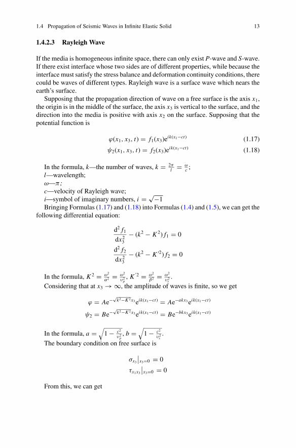
1.4.2.3 Rayleigh Wave

If the media is homogeneous infinite space, there can only exist P-wave and S-wave.If there exist interface whose two sides are of different properties, while because theinterface must satisfy the stress balance and deformation continuity conditions, therecould be waves of different types. Rayleigh wave is a surface wave which nears theearth’s surface.

Supposing that the propagation direction of wave on a free surface is the axis x1,the origin is in the middle of the surface, the axis x3 is vertical to the surface, and thedirection into the media is positive with axis x2 on the surface. Supposing that thepotential function is

ϕ(x1, x3, t) � f1(x3)eik(x1−ct) (1.17)

ψ2(x1, x3, t) � f2(x3)eik(x1−ct) (1.18)

In the formula, k—the number of waves, k � 2πl � ω

c ;l—wavelength;ω—π ;c—velocity of Rayleigh wave;i—symbol of imaginary numbers, i � √−1Bringing Formulas (1.17) and (1.18) into Formulas (1.4) and (1.5), we can get the

following differential equation:

d2 f1dx23

− (k2 − K 2) f1 � 0

d2 f2dx23

− (k2 − K ′2) f2 � 0

In the formula, K 2 � ω2

α2 � ω2

υ2p, K

′2 � ω2

β2 � ω2

υ2s.

Considering that at x3 → ∞, the amplitude of waves is finite, so we get

ϕ � Ae−√k2−K 2x3eik(x1−ct) � Ae−akx3eik(x1−ct)

ψ2 � Be−√k2−K 2x3eik(x1−ct) � Be−bkx3eik(x1−ct)

In the formula, a �√1 − c2

υ2p, b �

√1 − c2

υ2s.

The boundary condition on free surface is

σx3

∣∣x3�0 � 0

τx1x3∣∣x3�0 � 0

From this, we can get


(1 + b2)A + i2bB � 0

− i2aA + (1 + b2)B � 0

In the formulas, the condition of A and B has untrivial solution as its determinantof coefficient being zero, thus we can get (1 + b2)2 − 4ab � 0.

Or this can be written as(2 − c2

υ2s

)2 � 4√1 − c2

υ2s

√1 − c2

υ2p.

Through squaring the two sides of the formula and arrangement, we can get

(c

υs

)6

− 8

(c

υs

)4

+

(24 − 16

υ2s

υ2p

)(c

υs

)2

− 16

(1 − υ2

s

υ2p

)� 0 (1.19)

Formula (1.19) can be further written as

(c

υs

)6

− 8

(c

υs

)4

+ 82 − υ

1 − υ

(c

υs

)2

− 8

1 − υ� 0 (1.20)

Formula (1.20) is a cubic equation of(

cυs

)2, so there at least exists one positive

root in 0 < c < υs < υp. If the value of the Poisson’s ratio v is given, the velocityvalue c of the correspondent Rayleigh wave could be found, which is denoted as υR ,and the solution of Formula (1.20) can be approximately expressed as

υR ≈ 0.862 + 1.14ν

1 + νυs (1.21)

If the potential function is given, we can get that the displacement is

u1 � i f1(x3)eik(x1−ct) (1.22a)

u2 � 0 (1.22b)

u3 � i f2(x3)eik(x1−ct) (1.22c)

in which,

f1(x3) � −Ak

(e−akx3 − 1 + b2

2be−bkx3

)

f2(x3) � Ak

(−ae−akx3 − 1 + b2

2be−bkx3

)

If consideration is only paid to the real component of displacement components,there is

u21f 21 (x3)

+u23

f 22 (x3)� 1 (1.23)


Fig. 1.7 Changes and trajectory of the displacement of Rayleigh wave in horizontal and verticaldirections along vertical direction

which shows that the trajectory of a particle is an oval in a plane surface of x1−x3, andits axial lengths in horizontal direction x1 and vertical direction x3 are, respectively,f1(x3) and f2(x3). Therefore, Rayleigh wave is a kind of elliptic polarized wave.When the Poisson’s ratio v is 0. 25, the changes and trajectory of the displace-

ment of Rayleigh wave in horizontal and vertical directions along vertical directionare shown in Fig. 1.7. It can be seen from the figure that the changes of horizon-tal displacement along the vertical direction are accompanied with reversal, whichmeans that, hereupon, the trajectory of the particle changes from retrograde ellipseto forward ellipse; the attenuation of Rayleigh wave is quite fast, with 1/5 attenuationafter each wavelength. Rayleigh wave is formed by reflection stack after body wavearriving at the earth’s surface, which is rare around the focus, and appears until theepicentral distance over VRh/(V2p − V2s)1/2 (h is the focal depth).

1.4.2.4 Love Wave

Love wave is another kind of surface wave, which was discovered by real seismicobservation, and its existence was then proved by A. E. H. Love in theory. Thecondition for the existence of Love wave is a loose horizontal cover layer existing insemi-infinite space. Love wave is a kind of SH wave.

Suppose that the origin is on the surface between the cover layer and the lowersemi-infinite body, where the axis x1 is the wave propagation direction, x3 is thevertical direction, the positive direction is forward inside the infinite body, and thewidth of the cover layer isH. Suppose that the displacement function is

⎧⎪⎪⎨⎪⎪⎩

u2(x1, x3, t) � f1(x3)eik(x−ct), −H ≤ x3 ≤ 0

u2(x1, x3, t) � f2(x3)eik(x−ct), x3 ≥ 0

u1 � u3 � 0

(1.24)


In the function, c is velocity of Love wave, c � ωk .

According to the boundary conditions of surface of x3 � 0 between the freesurface x3 � −H with the cover layer and the lower infinite body, and the amplitude( f2(∞)) should be bounded at infinite depth (x3 � ∞), the physical conditions ofthe existence of Love wave can be worked out as

ν2

√1 − c2

υ2s2

� ν1

√c2

υ2s2

− 1 tan

(ωH

c

√c2

υ2s1

− 1

)(1.25)

In the formula, υs1, ν1 is the shear wave speed and the Poisson’s ratio of the coverlayer;

υs2, ν2 is the shear wave speed and the Poisson’s ratio of the lower semi-infinitebody.

Thus it can be concluded that if υs1 < c < υs2, Formula (1.25) could be satisfied.Therefore, Love wave could only exist when the shear speed of cover layer is lessthan that of the lower semi-infinite body.

1.4.2.5 Dispersion Relation and Group Velocity

It could be seen from above that there is only one speed of S-wave or P-waveon homogeneous elastic surface, which completely depends on the property of themedia. However, the propagation of surface wave could not be described solely withvelocity in the layered elastic media, and there is relation c � ω

k among the wavevelocity c, frequency ω, and wavenumber k, which is called dispersion relation.Thus, it is clear that the simple harmonic surface wave with different wavenumber orfrequency propagates with different velocity. The velocity c of each simple harmonicsurface wave is called phase velocity.

However, c is not the ideal wave parameter to describe the propagation of surfacewave, because the key feature of wave motion is the propagation of wave motionenergy, which is not the phase velocity. If the propagation of a number of simpleharmonic surfacewavewith similar wavenumber k or frequencyω is investigated, theresult of them superimposing together is to form a wave packet, and the propagationvelocity of the wave packet is different from the phase velocity of single simpleharmonic surface wave. Due to that the energy of wave motion depends on theamplitude when the frequency is the same, so the propagation velocity of wavepacket is that of wave motion energy. Thus, the propagation of wave packet is calledgroup velocity cg .

1.5 Reflection and Refraction of Seismic Wave 17

1.5 Reflection and Refraction of Seismic Wave

1.5.1 Reflection of Seismic Wave on Free Surface

1.5.1.1 SH Wave

Suppose that the uplink SH plane harmonic wave u2i in homogeneous elastic mediawith x3 > 0 enters the free surface x3 � 0 with incidence angle φ (see Fig. 1.8), u2icould be written as

u2i � Eei(ωt−k1x1+k2x3) (1.26)

In the formula,

k1 � k sin φ � ω

υssin φ

k2 � k cosφ � ω

υscosφ

The general solution of plane harmonic wave in the homogeneous elastic mediagiven by Formula (1.26) could be expressed as

u2 � Eei(ωt−k1x1+k2x3) + Fei(ωt−k1x1−k2x3) (1.27)

In Formula (1.27), the first item is the incident wave u2i , and the second wave isthe reflected wave u2r . The amplitude coefficient of u2r , F could be determined bycondition τ23

∣∣x3�0 of the free surface. From this, we can get

E � F (1.28)

Fig. 1.8 SH waves are reflected on free surface


Thus, substituting Formulas (1.28) into (1.27), we can get

u2 � 2Eei(ωt−k1x1) cos(k2x3) (1.29)

When x3 � 0, there is

u2i � Eei(ωt−k1x1) (1.30)

u2 � 2Eei(ωt−k1x1) (1.31)

It can be known from Formulas (1.30) and (1.31) that

u2u2i

� u2u2i

� u2u2i

� 2 (1.32)

It can thus be seen that, no matter how much the incident angle φ and incidentwave frequency are, when wave enters the free surface, the motion of the free surfacealways doubles that of the incident wave.

1.5.1.2 P-Wave

Suppose that the uplink P plane harmonic wave ϕi in homogeneous elastic mediaenters the free surface x3 � 0 with incidence angle θ (see Fig. 1.9), ϕi could bewritten as

ϕi � Epei(ωt−k1p x1+k2px3) (1.33)

In the formula,

k1p � kp sin θ � ω

υpsin θ (1.34)

Fig. 1.9 P-waves arereflected on free surface


k2p �

⎧⎪⎪⎪⎪⎨⎪⎪⎪⎪⎩

√(ωυp

)2 − k21p k1p ≤ ωυp

−i

√k21p −

(ωυp

)2k1p > ω

υp

(1.35)

With respect to in-plane wave motion, the total wave field is generally composedof potential of P-wave ϕ and that of S-wave ψ . The general solution of their planeharmonic wave in the homogeneous elastic media could be expressed as

ϕ � Epei(ωt−k1px1+k2px3) + Fpe

i(ωt−k1p x1−k2p x3) (1.36a)

ψ � Fsei(ωt−k1s x1−k2s x3) (1.36b)

In the formula,

k1s � ks sin φ � ω

υssin φ (1.37)

k2s �

⎧⎪⎪⎪⎪⎨⎪⎪⎪⎪⎩

√(ωυs

)2 − k21s k1s ≤ ωυs

−i

√k21s −

(ωυs

)2k1s > ω

υs

(1.38)

In Formula (1.36a), the first item is the incident wave ϕi , and the second wave isthe reflected P-wave ϕr . In the general solution Formula (1.36b) of S-wave potentialψ , the uplink item is omitted because there exists no SV wave entering the freesurface. According to the conditions of free surface:

when x3 � 0,

σ3 � 0 τ13 � 0 (1.39)

It is easy to see that if the conditional Formula (1.39) of free surface of x3 � 0 isto be satisfied at any time, it must meet k1p � k1s ; that is, the apparent velocity ofall harmonious wave propagating along the axis x1 must the same, i.e.

υp

sin θ� υs

sin φ(1.40)

Formula (1.40) is a form of Snell law in elastic media. Therefore, it could berecorded as. Thus, it can be concluded from Formula (1.40) that

(υs

υp

)2

sin 2θ (Ep − Fp) − cos 2φFs � 0 (1.41a)

cos 2φ(Ep+Fp) − sin 2θFs � 0 (1.42b)


From this, we can get

Fp

Ep� υ2

s sin 2θ sin 2φ − υ2p cos

2 2φ

υ2s sin 2θ sin 2φ + υ2

p cos2 2φ

(1.43a)

Fs

Ep� 2υ2

s sin 2θ sin 2φ

υ2s sin 2θ sin 2φ + υ2

p cos2 2φ

(1.43b)

In the formula,

⎧⎪⎪⎪⎨⎪⎪⎪⎩

sin 2φ � 2 sin φ cosφ � 2 υsυp

sin θ

√1 −

(υsυp

)2sin2 θ

cos 2φ � 1 − 2 sin2 φ � 1 −(

υsυp

)2sin2 θ

(1.44)

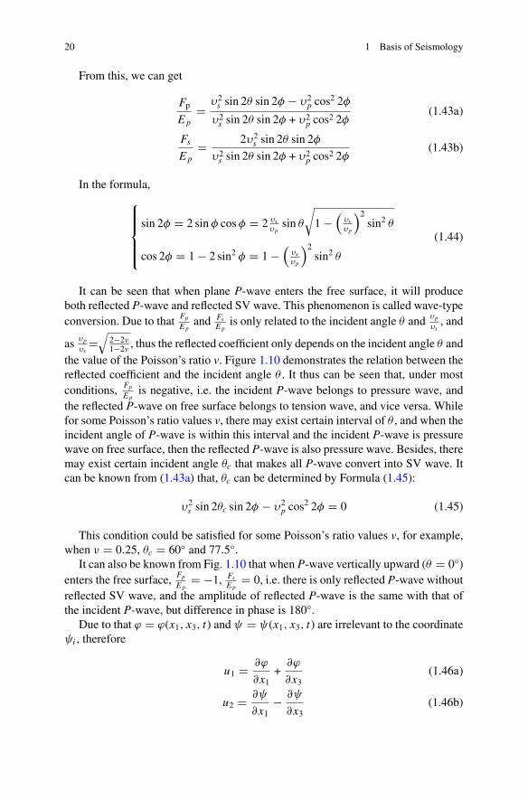
It can be seen that when plane P-wave enters the free surface, it will produceboth reflected P-wave and reflected SV wave. This phenomenon is called wave-typeconversion. Due to that Fp

Epand Fs

Epis only related to the incident angle θ and υp

υs, and

as υp

υs�

√2−2ν1−2ν , thus the reflected coefficient only depends on the incident angle θ and

the value of the Poisson’s ratio v. Figure 1.10 demonstrates the relation between thereflected coefficient and the incident angle θ . It thus can be seen that, under mostconditions, Fp

Epis negative, i.e. the incident P-wave belongs to pressure wave, and

the reflected P-wave on free surface belongs to tension wave, and vice versa. Whilefor some Poisson’s ratio values v, there may exist certain interval of θ , and when theincident angle of P-wave is within this interval and the incident P-wave is pressurewave on free surface, then the reflected P-wave is also pressure wave. Besides, theremay exist certain incident angle θc that makes all P-wave convert into SV wave. Itcan be known from (1.43a) that, θc can be determined by Formula (1.45):

υ2s sin 2θc sin 2φ − υ2

p cos2 2φ � 0 (1.45)

This condition could be satisfied for some Poisson’s ratio values v, for example,when ν � 0.25, θc � 60◦ and 77.5◦.

It can also be known from Fig. 1.10 that when P-wave vertically upward (θ � 0◦)enters the free surface, Fp

Ep� −1, Fs

Ep� 0, i.e. there is only reflected P-wave without

reflected SV wave, and the amplitude of reflected P-wave is the same with that ofthe incident P-wave, but difference in phase is 180◦.

Due to that ϕ � ϕ(x1, x3, t) and ψ � ψ(x1, x3, t) are irrelevant to the coordinateψi , therefore

u1 � ∂ϕ

∂x1+

∂ϕ

∂x3(1.46a)

u2 � ∂ψ

∂x1− ∂ψ

∂x3(1.46b)


Fig. 1.10 Reflected coefficient of the incident P-wave on free surface

u3 � ∂ϕ

∂x3− ∂ψ

∂x1(1.46c)

1.5.1.3 SV Wave

Suppose that the uplink SV plane harmonic wave ψi enters the free surface x3 � 0with incidence angle φ (see Fig. 1.11):

ψi � Esei(ωt−k1x1+k2s x3) (1.47)

Then the general solution of the potential of total wave field is

ϕr � Fpei(ωt−k1x1)e

− ωυs

√sin2 φ−

(υsυp

)2x3

(1.48)

ϕ � Esei(ωt−k1x1+k2s x3) + Fse

i(ωt−k1x1−k2s x3) (1.49)

changwei yang · guotao yang jianjing zhang · hongsheng ma

Documents