channel capacity - babeș-bolyai universitymath.ubbcluj.ro/~tradu/ti/coverch7_article.pdf ·...
TRANSCRIPT
Channel CapacityThe Characterization of the Channel Capacity
Radu T. Trımbitas
November 2012
Outline
Contents
1 Channel Capacity 21.1 Introduction . . . . . . . . . . . . . . . . . . . . . . . . . . . . . . 21.2 Discrete Channels . . . . . . . . . . . . . . . . . . . . . . . . . . . 5
2 Examples of Channel Capacity 82.1 Noiseless Binary Channel . . . . . . . . . . . . . . . . . . . . . . 82.2 Noisy Channel with non-overlapping outputs . . . . . . . . . . 92.3 Permutation Channel . . . . . . . . . . . . . . . . . . . . . . . . . 92.4 Noisy Typewriter . . . . . . . . . . . . . . . . . . . . . . . . . . . 102.5 Binary Symmetric Channel (BSC) . . . . . . . . . . . . . . . . . . 122.6 Binary Erasure Channel . . . . . . . . . . . . . . . . . . . . . . . 13
3 Symmetric Channels 15
4 Properties of Channel Capacity 16
5 The Shannon’s 2nd Theorem 165.1 The Shannon’s 2nd Theorem - Intuition . . . . . . . . . . . . . . 165.2 Definitions . . . . . . . . . . . . . . . . . . . . . . . . . . . . . . . 185.3 Jointly Typical Sequences . . . . . . . . . . . . . . . . . . . . . . 20
6 Channel Coding Theorem 246.1 Channel Coding Theorem . . . . . . . . . . . . . . . . . . . . . . 246.2 Zero-Error Codes . . . . . . . . . . . . . . . . . . . . . . . . . . . 346.3 Fano’s Lemmas . . . . . . . . . . . . . . . . . . . . . . . . . . . . 346.4 Converse to the Channel Coding Theorem . . . . . . . . . . . . . 356.5 Equality in the Converse to the Channel Coding Theorem . . . . 36
7 Feedback Capacity 37
1

8 Source-Channel Separation Theorem 39
9 Coding 429.1 Introduction to coding . . . . . . . . . . . . . . . . . . . . . . . . 429.2 Hamming Codes . . . . . . . . . . . . . . . . . . . . . . . . . . . 44
1 Channel Capacity
1.1 Introduction
Towards Channels
• So far, we have been talking about compression. I.e., we have somesource p(x) with information H(X) (the limits of compression) and thegoal is to compress it down to H bits per source symbol in a representa-tion Y.
• In some sense, the compressed representation has a ”capacity” which isthe total amount of bits that can be represented. I.e., with n bits, we canobviously represent no more than n bits of information.
• Compression can be seen as a process where we want to fully utilize thecapacity in the compressed representation, i.e., if we have n bits of codeword, we ideally (i.e., in an perfect compression scheme) would like thereto be no less than n bits of information being represented. Recall effi-ciency: H(X) = E(`).
• We now want to transmit information over a channel.
• From Claude Shannon: The fundamental problem of communication isthat of reproducing at one point either exactly or approximately a mes-sage selected at another point. Frequently the messages have meaning . .. [which is] irrelevant to the engineering problem
• Is there a limit to the rate of communication over a channel?
• If the channel is noisy, can we achieve (essentially) perfect error-free trans-mission at a reasonable rate?
2

The 1930s America
• Stock-market crash of 1929
• The great depression
• Terrible conditions in textile and mining industries
• deflated crop prices, soil depletion, farm mechanization
• The rise of fascism and the Nazi state in Europe.
• Analog radio, and urgent need for secure, precise, and efficient commu-nications
• Radio communication, noise always in data transmission (except for Morsecode, which is slow).
Radio Communications
• Place yourself back in the 1930s.
• Analog communication model of the 1930s.
• Q: Can we achieve perfect communication with an imperfect communi-cation channel?
3

• Q: Is there an upper bound on the information capable of being sent un-der different noise conditions?
• Key: If we increase the transmission rate over a noisy channel will theerror rate increase?
• Perhaps the only way to achieve error free communication is to have arate of zero.
• The error profile we might expect to see is the following:
• Here, probability of error Pe goes up linearly with the rate R, with anintercept at zero.
• This was the prevailing wisdom at the time. Shannon was critical inchanging that.
Simple Example
• Consider representing a signal by a sequence of numbers.
• We now know that any signal (either inherently discrete or continuous,under the right conditions) can be perfectly represented (or at least ar-bitrarily well) by a sequence of discrete numbers, and they can even bebinary digits.
• Now consider speaking such a sequence over a noisy AM channel.
• Very possible one number will be masked by noise.
• In such case, each number we repeat k times, where k is sufficiently largeto ensure we can ”decode” the original sequence with very small proba-bility of error.
• Rate of this code decreases but we can communicate reliably even if thechannel is very noisy.
• Compare this idea to the figure on the following page.
4

A key idea
• If we choose the messages carefully at the sender, then with very highprobability, they will be uniquely identifiable at the receiver.
• The idea is that we choose the source messages that (tend to) not haveany ambiguity (or have any overlap) at the receiver end. I.e.,
• This might restrict our possible set of source messages (in some casesseverely, and thereby decrease our rate R), but if any message received ina region corresponds to only one source message, ”perfect” communica-tion can be achieved.
1.2 Discrete Channels
Discrete Channels
Definition 1. A discrete channel is a system consisting of an input alphabet X ,an output alphabet Y , and a distribution (probability transition matrix) p(y|x)which is the probability of observing output symbol y given that we send thesymbol x. A discrete channel is memoryless if the probability distribution of yt,the output at time t, depends only on the input xt and is independent of allprevious inputs x1:t−1.
• We will see many instances of discrete memoryless channels (or just DMC).
• Recall back from lecture 1 our general model of communications:
Model of Communication
• Source message W, one of M messages.
• Encoder transforms this into a length-n string of source symbols Xn
5

• Noisy channel distorts this message into a length-n string of receiver sym-bols Yn.
• Decoder attempts to reconstruct original message as best as possible, comesup with W, one of M possible sent messages.
Rates and Capacities
• So we have a source X governed by p(x) and channel that transforms Xsymbols to Y symbols and which is governed by the conditional distri-bution p(y|x)
• These two items p(x) and p(y|x) are sufficient to compute the mutualinformation between X and Y. That is, we compute
I(X; Y) = Ip(x)(X, Y) = ∑x,y
p(x)p(y|x)︸ ︷︷ ︸p(x,y)
logp(y|x)p(y)
(1)
= ∑x,y
p(x)p(y|x) logp(y|x)
∑x′ p(y|x′)p(x′)(2)
• We write this as I(X; Y) = Ip(x)(X; Y), meaning implicitly the MI quan-tity is a function of the entire distribution p(x), for a given fixed channelp(y|x).
• We will often be optimizing over the input distribution p(x) for a givenfixed channel p(y|x).
Definition 2 (Information flow). The rate of information flow through a channelis given by I(X; Y), the mutual information between X and Y, in units of bitsper channel use.
Definition 3 (Capacity). The information capacity of a channel is the maximuminformation flow
C = maxp(x)
I(X; Y), (3)
where the maximum is taken over all possible input distributions p(x).
6

Definition 4 (Rate). The rate R of a code is measured in the number of bits perchannel use.
• We shall soon give an operational definition of channel capacity as thehighest rate in bits per channel use at which information can be sent witharbitrarily low probability of error.
• Shannon’s second theorem establishes that the information channel ca-pacity is equal to the operational channel capacity.
• There is a duality between the problems of data compression and datatransmission.
– During compression, we remove all the redundancy in the data toform the most compressed version possible
– During data transmission, we add redundancy in a controlled fash-ion to combat errors in the channel.
• We show that a general communication system can be broken into twoparts and that the problems of data compression and data transmissioncan be considered separately.
Fundamental Limits of Compression
• For compression, if error exponent is positive, then error→ 0 exponen-tially fast as block length→ 1. Note, Pe ∼ e−nE(R).
• That is,
• Only hope of reducing error was if R > H. Something ”funny” happensat the entropy rate of the source distribution. Can’t compress below thiswithout incurring error.
Fundamental Limits of Data Transmission/Communication
• For communication, lower bound on probability of error becomes boundedaway from 0 as the rate of the code R goes above a fundamental quantityC. Note, Pe ∼ e−nE(R).
7
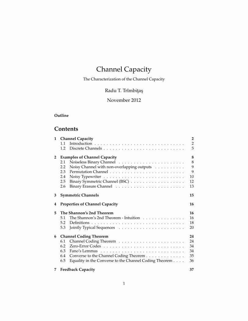
• That is,
• only possible way to get low error is if R < C. Something funny happensat the point C, the capacity of the channel.
• Note that C is not 0, so can still achieve ”perfect” communication over anoisy channel as long as R < C.
2 Examples of Channel Capacity
2.1 Noiseless Binary Channel
Noiseless Binary Channel
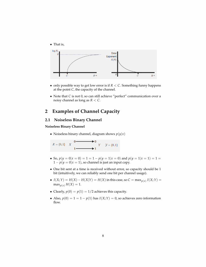
• Noiseless binary channel, diagram shows p(y|x)
• So, p(y = 0|x = 0) = 1 = 1− p(y = 1|x = 0) and p(y = 1|x = 1) = 1 =1− p(y = 0|x = 1), so channel is just an input copy.
• One bit sent at a time is received without error, so capacity should be 1bit (intuitively, we can reliably send one bit per channel usage).
• I(X; Y) = H(X)−H(X|Y) = H(X) in this case, so C = maxp(x) I(X; Y) =maxp(x) H(X) = 1.
• Clearly, p(0) = p(1) = 1/2 achieves this capacity.
• Also, p(0) = 1 = 1− p(1) has I(X; Y) = 0, so achieves zero informationflow.
8

2.2 Noisy Channel with non-overlapping outputs
Noisy Channel with non-overlapping outputsThis channel has 2 possible outputs corresponding to each of the 2 inputs.
The channel appears to be noisy, but really is not.
• Here, p(y = 0|x = 0) = p(y = 1|x = 0) = 1/2 and p(y = 2|y = 1) =p(y = 3|x = 1) = 1/2.
• If we receive a 0 or 1, we know 0 was sent. If we receive a 2 or 3, a 1 wassent.
• Thus, C = 1 since only two possible error free messages.
• Same argument applies
I(X; Y) = H(X)− H(Y|X)︸ ︷︷ ︸=0
= H(X)
• Again uniform distribution p(0) = p(1) = 1/2 achieves the capacity.
2.3 Permutation Channel
Permutation Channel
• Here, p(Y = 1|X = 0) = p(Y = 0|X = 1) = 1.
• So output is a binary permutation (swap) of input.
• Thus, C = 1; no information lost.
• In general, for alphabet of size k = |X | = |Y|, let be a permutation, sothat Y = σ(X).
• Then C = log k.
9

Asside: on the optimization to compute the value C
• To maximize a given function f (x), it is sufficient to show that f (x) ≤ αfor all x, and then find an x∗ such that f (x∗) = α.
• We’ll be doing this over the next few slides when we want to computeC = maxp(x) I(X; Y) for fixed p(y|x).
• The solution p∗(x) that we find that achieves this maximum won’t nec-essarily be unique.
• Also, the solution p∗(x) that we find won’t necessarily be the one that weend up, say, using when we wish to do channel coding.
• Right now C is just the result of a given optimization.
• We’ll see that C, as computed, is also the critical point for being able tochannel code with vanishingly small error probability.
• The resulting p∗(x) that we obtain as part of the optimization in orderto compute C won’t necessarily be the one that we use for actual coding(example forthcoming).
2.4 Noisy Typewriter
Figure 1: Noisy Typewriter, C = log 13 bits
10

Noisy Typewriter
• In this case the channel input is either received unchanged at the outputwith probability 1/2 or is transformed into the next letter with probabil-ity 1/2 (Figure 1).
• So 26 input symbols, and each symbol maps probabilistically to itself orits lexicographic neighbor.
• I.e., p(A→ A) = p(A→ B) = 1/2, etc.
• Each symbol always has some chance of error, so how can we communi-cate without error?
• Choose subset of symbols that can be uniquely disambiguated on re-ceiver side. Choose every other source symbol, A, C, E, etc.
• Thus A → {A; B}, C → {C; D}, E → {E; F}, etc. so that each receivedsymbols has only one unique source symbol.
• Capacity C = log 13
• Q: what happens to C when probabilities are not all 1/2?
• We can also compute the capacity more mathematically.
• For example:
C = maxp(x)
I(X; Y) = maxp(x)
(H(X)− H(Y|X)
= maxp(x)
H(Y)− 1 //for X = x ∃ 2 choices
= log 26− 1 = log 13
• The maxp(x) H(Y) = log 26 can be achieved by using the uniform distri-bution for p(x), for which when we choose any x symbol, there is equallikelihood of two Ys being received.
• An alternatively p(x) would put zero probability on the alternates (B, D,F, etc.). In this case, we still have H(Y) = log 26
• So the capacity is the same in each case (∃ two p(x) that achieved this)but only one is what we would use, say, for error free coding.
11

2.5 Binary Symmetric Channel (BSC)
Binary Symmetric Channel (BSC)
• A bit that is sent will be flipped with probability p.
• p(Y = 1|X = 0) = p = 1− p(Y = 0|X = 0). p(Y = 0|X = 1) = p =p(Y = 1|X = 1).
• BSC is the simplest model of channel with errors, yet it captures most ofthe complexity of the general problem
• Q: can we still achieve reliable (”guaranteed” error free) communicationwith this channel? A: Yes, if p < 1/2 and if we do not ask for too higha transmission rate (which would be R > C), then we can. Actually, anyp 6= 1/2 is sufficient.
• Intuition: think about AEP and/or block coding.
• But how to compute C, the capacity?
I(X; Y) = H(Y)− H(Y|X) = H(Y)−∑ p(x)H (Y|X = x)
= H(Y)−∑ p(x)H (p) = H(Y)− H (p) ≤ 1− H(p).
• When is H(Y) = 1? Note that
P(Y = 1) = P(Y = 1|X = 1)P(X = 1)+P(Y = 1|X = 0)P(X = 0)
= (1− p)P(X = 1) + pP(X = 1)= P(X = 1)
• So H(Y) = 1 if H(X) = 1.
• Thus, we get that C = 1− H(p) which happens when X is uniform.
• If p = 1/2 then C = 0, so if it randomly flips bits, then no informationcan be sent.
• If p 6= 1/2, then we can communicate, albeit potentially slowly. E.g., ifp = 0.499 then C = 2.8854× 10−6 bits per channel use. So to send onebit, need to use the channel quite a bit.
• If p = 0 or p = 1, then C = 1 and we can get maximum possible rate (i.e.,the capacity is one bit per channel use).
12

Decoding
• Lets temporarily look ahead to address this problem.
• We can ”decode” the source using the received string, source distribu-tion, and the channel model p(y|x) via Bayes rule. I.e.
P(X|Y) = P(Y|X)P(X)
P(Y)=
P(Y|X)P(X)
∑x′ P(Y|X′ = x′)Pr(X′ = x′)
• If we get a particular y, we can compute p(x|y) and make a decisionbased on that. I.e., x = argmaxx p(x|y).
• This is optimal decoding in that it minimizes the error.
• Error if x 6= x, and P(error) = P(x 6= x).
• This is minimal if we chose argmaxx p(x|y) since the error 1− P(x|y) isminimal.
Minimum Error Decoding
• Note: Computing quantities such as P(x|y) is a task of probabilistic in-ference.
• Often this problem is difficult (NP-hard). This means that doing mini-mum error decoding might very well be exponentially expensive (unlessP = NP).
• Many real world codes are such that computing the exact computationmust be approximated (i.e., no known fast algorithm for minimum erroror maximum likelihood decoding).
• Instead we do approximate inference algorithms (e.g., loopy belief prop-agation, message passing, etc.). These algorithms tend still to work verywell in practice (achieve close to the capacity C).
• But before doing that, we need first to study more channels and the the-oretical properties of the capacity C.
2.6 Binary Erasure Channel
Binary Erasure Channel
13

• e is an erasure symbol, if that happens we don’t have access to the trans-mitted bit.
• The probability of dropping a bit is then α.
• We want to compute capacity. Obviously, C = 1 if α = 0.
C = maxp(x)
I(X, Y) = maxp(x)
(H(Y)− H(X|Y))
= maxp(x)
H(Y)− H(α).
• So while H(Y) ≤ log 3, we want actual value of the capacity.
• let E = {Y = e}. Then
H(Y) = H(Y, E) = H(E) + H(Y|E).
• Let π = P(X = 1). Then
H(Y) = H
if Y=0︷ ︸︸ ︷(1− π)(1− α),
if Y=e︷︸︸︷α ,
if Y=1︷ ︸︸ ︷π(1− α)
= H(α) + (1− α)H(π).
• This last equality follows since H(E) = H(α), and
H(Y|E) = H(Y|Y = e) + (1− α)H(Y|Y 6= e) = α · 0 + (1− α)H(π).
• Then we get
C = maxp(x)
H(Y)− H(α)
= maxπ
((1− α) H(π) + H(α))− H(α)
= maxπ
(1− α) H(π) = 1− α
• Best capacity when π = 1/2 = P(X = 1) = P(X = 0).
• This makes sense, loose α% of the bits of original capacity.
14

3 Symmetric Channels
Symmetric Channels
Definition 5. A channel is symmetric if rows of the channel transition matrixp(y|x) are permutations of each other, and columns of this matrix are permu-tations of each other. A channel is weakly symmetric if every row of the tran-sition matrix p(.|x) is a permutation of every other row, and all column sums∑x p(y|x) are equal.
Theorem 6. For a weakly symmetric channel,
C = log |Y| − H(r) (4)
where r is the row of transition matrix. This is achieved by a uniform distribution onthe input alphabet.
Proof.
I(X; Y) = H(Y)− H(Y|X) = H(Y)− H(r) ≤ log |Y| − H(r) (5)
with equality if the output distribution is uniform. But p(x) = 1/ |X | achievesa uniform distribution on Y, as seen from
p(y) = ∑x∈X
p(y|x)p(x) =1|X |∑ p(y|x) = c
1|X | =
1|Y| , (6)
where c is the sum of the entries in one column of the transition matrix.
Example 7. The channel with transition matrix
p(y|x) =
0.3 0.2 0.50.5 0.3 0.20.2 0.5 0.3
is symmetric. Its capacity is C = log 3− H(0.5, 0.2, 0.3) = 8.8818× 10⁻¹⁶.
Example 8. Y = X + Z (mod c), where X = Z = {0, 1, . . . , c− 1}, and X andZ are independent.
Example 9. The channel with transition matrix
p(y|x) =[ 1
316
12
13
12
16
]is weakly symmetric, but not symmetric.
15

4 Properties of Channel Capacity
Properties of Channel Capacity
1. C ≥ 0 since I(X; Y) ≥ 0.
2. C ≤ log |X | since C = maxp(x) I(X; Y) ≤ max H(X) = log |X |.
3. C ≤ log |Y| for the same reason. Thus, the alphabet sizes limit the trans-mission rate.
4. I(X; Y) = Ip(x)(X; Y) is a continuous function of p(x).
5. I(X; Y) is a concave function of p(x) for fixed p(y|x).
6. Thus, Iλp1+(1−λ)p2(X; Y) ≥ λIp1(X; Y) + (1− λ)Ip2(X; Y). Interestingly,
since concave, this makes computing something like the capacity easier.I.e., a local maximum is a global maximum, and computing the capacityfor a general channel model is a convex optimization procedure.
7. Recall also, I(X; Y) is a convex function of p(y|x) for fixed p(x).
5 The Shannon’s 2nd Theorem
5.1 The Shannon’s 2nd Theorem - Intuition
Shannon’s 2nd Theorem
• One of the most important theorems of the last century.
• We’ll see it in various forms, but we state it here somewhat informally tostart acquiring intuition.
Theorem 10 (Shannon’s 2nd Theorem). C is the maximum number of bits (onaverage, per channel use) that we can transmit over a channel reliably.
• Here, ”reliably” means with vanishingly small and exponentially decreas-ing probability of error as the block length gets longer. We can easilymake this probability essentially zero.
• Conversely, if we try to push > C bits through the channel, error quicklygoes to 1.
• Intuition of this we’ve already seen in the noisy typewriter and the regionpartitioning.
• Slightly more precisely, this is a sort of bin packing problem.
• We’ve got a region of possible codewords, and we pack as many smallernon-overlapping bins into the region as possible.
16

• The smaller bins correspond to the noise in the channel, and the packingproblem depends on the underlying ”shape”
• Not really a partition, since there might be wasted space, also dependingon the bin and region shapes.
• Intuitive idea: use typicality argument.
• There are ≈ 2nH(X) typical sequences, each with probability 2−nH(X) andwith p(A(n)
ε ) ≈ 1, so the only thing with ”any” probability is the typicalset and it has all the probability.
• The same thing is true for conditional entropy.
• That is, for a typical input X, there are 2nH(Y|X) output sequences.
• Overall, there are 2nH(Y) typical output sequences, and we know that2nH(Y) ≥ 2nH(Y|X).
Shannon’s 2nd Theorem: Intuition
• Goal: find a non-confusable subset of the inputs that produce disjointoutput sequences (as in picture).
• There are ≈ 2nH(Y) (typical) outputs (i.e., the marginally typical Y se-quences).
• There are 2nH(Y|X) (X-conditionally typical Y sequences) outputs. ≡ theaverage possible number of outputs for a possible input, so this manycould be confused with each other. I.e., on average, for a given X = x,this is approximately how many outputs there might be.
• So the number of non-confusable inputs is
≤ 2nH(Y)
2nH(Y|X)= 2n(H(Y)−H(Y|X)) = 2nI(X;Y) (7)
• Note, in non-ideal case, there could be overlap of the typical Y-given-Xsequences, but the best we can do (in terms of maximizing the number ofnon-confusable inputs) is when there is no overlap on the output. This isassumed in the above.
17

• We can view the number of non-confusable inputs (7) as a volume. 2nH(Y)
is the total number of possible slots, while 2nH(Y|X) is the number of slotstaken up (on average) for a given source word. Thus, the number ofsource words that can be used is the ratio.
• To maximize the number of non-confusable inputs (7), for a fixed channelp(y|x), we find the best p(x) which gives I(X; Y) = C, which is the logof the maximum number of inputs possible to use.
• This is the capacity.
5.2 Definitions
Definitions
Definitions 11. • Message W ∈ {1, . . . , M} requiring log M bits per mes-sage.
• Signal sent through channel Xn(W), a random codeword.
• Received signal from channel Y ∼ p(yn|xn)
• Decoding via guess W = g(Yn).
• Discrete memoryless channel (DMC) (X ; p(y|x);Y)
Definitions 12. • n-th extension to channel is (X n; p(yn|xn);Yn), where
p(
yk|xk, yk−1)= p(xk|yk)
• Feedback if xk can use both previous inputs and outputs.
18

• No feedback if p(xk|x1:k−1; y1:k−1) = p(xk|x1:k−1). We’ll analyze feedbacka bit later.
Remark. If the channel is used without feedback, the channel transitionfunction reduces to
p (yn|xn) =n
∏i=1
p(yi|xi). (8)
(M,n) code
Definition 13 ((M, n) code). An (M, n) code for channel (X ; p(y|x);Y) is
1. An index set {1, 2, . . . , M} .
2. An encoding function Xn : {1, 2, . . . , M} → X n yielding codewordsXn(1), Xn(2), Xn(3), . . . , Xn(M). Each source message has a codeword,and each codeword is n code symbols.
3. Decoding function, i.e., g : Yn → {1, 2, . . . , M} which makes a ”guess”about original message given channel output.
Remark. In an (M, n) code, M = the number of possible messages to besent, and n = number of channel uses by the codewords of the code.
Error
Definition 14 (Probability of Error λi for message i ∈ {1, . . . , M}).
λi := P (g(Yn) 6= i|Xn = xn(i)) = ∑yn
p (yn|xn(i)) I (g (yn) 6= i) (9)
I(·) is the indicator function; the conditional probability of error given thatindex i was sent.
Definition 15 (Max probability of Error λ(n) for (M, n) code).
λ(n) := maxi∈{1,2,...,M}
λi. (10)
Definition 16 (Average probability of error P(n)e ).
P(n)e =
1M
M
∑i=1
λi = P(Z 6= g(Yn))
where Z is a r.v. with probability P(Z = i) ∼ U(M) (discrete uniform)
P(n)e = E(I(Z 6= g(Yn))) =
M
∑i=1
P (g(Yn) 6= i|Xn = Xn(i)) p(i),
where p(i) = 1M .
Remark. A key Shannon’s result is that a small average probability of errormeans we must have a small maximum probability of error!
19

Rate
Definition 17. The rate R of an (M, n) code is
R =log M
nbits per transmission
Definition 18. A rate R is achievable if there exists a sequence of(⌈
2nR⌉ , n)
codes such that λ(n) → 0 as n→ ∞.
Remark. To simplify the notation we write(2nR, n
)instead
(⌈2nR⌉ , n
).
Capacity
Definition 19. The capacity of a channel is the supremum of all achievable rates.
• So the capacity of a DMC is the rate beyond which the error won’t tendto zero with increasing n.
• Note: this is a different notion of capacity that we encountered before.
• Before we defined C = maxp(x) I(X, Y).
• Here we are defining something called the ”capacity of a DMC”.
• We have not yet compared the two (but of course we will ).
5.3 Jointly Typical Sequences
Jointly Typical Sequences
Definition 20. The set of jointly typical sequences with respect to the distribu-tion p(x, y) is defined by
A(n)ε = {(xn, yn) ∈ X n ×Yn :∣∣∣∣− 1
nlog p(xn)− H(X)
∣∣∣∣ < ε (11)∣∣∣∣− 1n
log p(yn)− H(Y)∣∣∣∣ < ε (12)∣∣∣∣− 1
nlog p(xn, yn)− H(X, Y)
∣∣∣∣ < ε
}, (13)
where
p(xn, yn) =n
∏i=1
p(xi, yi). (14)
Jointly Typical Sequences: Picture
20

Intuition for Jointly Typical Sequences
• So intuitively,
num. jointly typical seqs.num ind. chosen typical seqs.
=2nH(X,Y)
2nH(X)2nH(Y)
= 2n(H(X,Y)−H(X)−H(Y))
= 2−nI(X,Y)
• So if we independently at random choose two (singly) typical sequencesfor X and Y, then the chance that it will be an (X, Y) jointly typical se-quence decreases exponentially with n, as long as I(X, Y) > 0.
• to decrease this chance as much as possible, it can become 2−nC.
Theorem 21 (Joint AEP). Let (Xn, Yn) ∼ p(xn, yn) = ∏ni=1 p(xi, yi) i.i.d. Then:
1. P((Xn, Yn) ∈ A(n)
ε
)→ 1 as n→ ∞.
2. (1− ε)2n(H(X,Y)−ε) ≤∣∣∣A(n)
ε
∣∣∣ ≤ 2n(H(X,Y)+ε)
3. If (Xn, Yn) ∼ p(xn)p(yn), are drawn independently, then
P((Xn, Yn) ∈ A(n)
ε
)≤ 2−n(I(X;Y)−3ε). (15)
Also, for sufficiently large n,
P((Xn, Yn) ∈ A(n)
ε
)≥ (1− ε) 2−n(I(X;Y)+3ε) (16)
21

Key property: we have bound on the probability of independently drawnsequences being jointly typical, falls off exponentially fast with n, if I(X; Y) >0.
Joint AEP proof
Proof of P((Xn, Yn) ∈ A(n)
ε
)→ 1. • We have, by the w.l.l.n.s,
− 1n
log P (Xn)→ −E (log P(X)) = H(X) (17)
so ∀ε > 0 ∃m1 such that for n > m1
P
∣∣∣∣− 1
nlog P(Xn)− H(X)
∣∣∣∣ > ε︸ ︷︷ ︸S1
<ε
3(18)
• So, S1 is a non-typical event.
Joint AEP proof
Proof of P((Xn, Yn) ∈ A(n)
ε
)→ 1. • Also ∃m2, m3 such that ∀n > m2 we
have
P
∣∣∣∣− 1
nlog P(Yn)− H(Y)
∣∣∣∣ > ε︸ ︷︷ ︸S2
<ε
3(19)
and ∀n > m3 we have
P
∣∣∣∣− 1
nlog P(Xn, Yn)− H(X, Y)
∣∣∣∣ > ε︸ ︷︷ ︸S3
<ε
3(20)
• So all events S1, S2 and S3 are non-typical events.
22

Joint AEP proof
Proof of P((Xn, Yn) ∈ A(n)
ε
)→ 1. • For n > max(m1, m2, m3), we have that
P (S1 ∪ S2 ∪ S3) ≤ 3ε/3
• So, non-typicality has probability < ε , meaning P(A(n)ε ) ≤ ε giving
P(A(n)ε ) ≥ 1− ε, as desired.
Joint AEP proof
Proof of (1− ε)2n(H(X,Y)−ε) ≤∣∣∣A(n)
ε
∣∣∣ ≤ 2n(H(X,Y)+ε). • We have
1 = ∑xn ,yn
p(xn, yn) ≥ ∑(xn ,yn)∈A(n)
ε
p(xn, yn) ≥∣∣∣A(n)
ε
∣∣∣ 2−n(H(X,Y)+ε)
=⇒∣∣∣A(n)
ε
∣∣∣ ≤ 2n(H(X,Y)+ε)
• Also, P(
A(n)ε
)> 1− ε,
1− ε ≤ ∑(xn ,yn)∈A(n)
ε
p(xn, yn) ≤∣∣∣A(n)
ε
∣∣∣ 2−n(H(X,Y)−ε)
=⇒∣∣∣A(n)
ε
∣∣∣ ≥ (1− ε)2n(H(X,Y)−ε)
Joint AEP proof
Proof of two indep. sequences are likely not jointly typical. We have the following twoderivations:
P((Xn, Yn)
)= ∑
(xn ,yn)∈A(n)ε
p(xn)p(yn)
≤ 2n(H(X,Y)+ε)2−n(H(X)−ε)2−n(H(Y)−ε)
= 2−n(I(X;Y)−3ε)
P((Xn, Yn)
)≥ (1− ε)2n(H(X,Y)−ε)2−n(H(X)+ε)2−n(H(Y)+ε)
= (1− ε)2−n(I(X;Y)+3ε).
23

More Intuition
• There are ≈ 2nH(X) typical X sequences
• There are ≈ 2nH(Y) typical Y sequences.
• The total number of independent typical pairs is ≈ 2nH(X)2nH(Y), but notall of them are jointly typical. Rather only ≈ 2nH(X;Y) of them are jointlytypical.
• The fraction of independent typical sequences that are jointly typical is:
2nH(X,Y)
2nH(X)2nH(Y)= 2n(H(X,Y)−H(X)−H(Y)) = 2−nI(X,Y)
and this is essentially the probability that a randomly chosen pair of(marginally) typical sequences is jointly typical.
• So if we use typicality to decode (which we will) then there are about2nI(X;Y) pairs of sequences before we start using pairs that will be jointlytypical and chosen randomly.
• Ex: if p(x) = 1/M then we can choose about M samples before we see agiven x, on average.
Channel Coding Theorem (Shannon 1948[2])
• The basic idea is to use joint typicality.
• Given a received codeword yn, find an xn that is jointly typical with yn.
• This xn will occur jointly with yn with probability 1, for large enough n.
• Also, the probability that some other xn is jointly typical with yn is about2−nI(X;Y),
• so if we use < 2nI(X; Y) codewords, then some other sequence beingjointly typical will occur with vanishingly small probability for large n.
6 Channel Coding Theorem
6.1 Channel Coding Theorem
Channel Coding Theorem (Shannon 1948): more formally
Theorem 22 (Channel coding theorem). For a discrete memoryless channel, allrates below capacity C are achievable. Specifically, for every rate R < C, there exists asequence of
(2nR, n
)codes with maximum probability of error λ(n) → 0 as n → ∞.
Conversely, any (2nR, n) sequence of codes with λ(n) → 0 as n → ∞ must have thatR < C.
24

Channel Theorem
• Implications: as long as we do not code above capacity we can, for allintents and purposes, code with zero error.
• This is true for all noisy channels representable under this model. We’retalking about discrete channels now, but we generalize this to continuouschannels in the coming lectures.
• We could look at error for a particular code and bound its errors.
• Instead, we look at the average probability of errors of all codes generatedrandomly.
• We then prove that this average error is small.
• This implies ∃many good codes to make the average small.
• To show that the maximum probability of error also small, we throwaway the worst 50% of the codes.
• Recall: idea is, for a given channel (X, p(y|x), Y) come up with a (2nR, n)code of rate R which means we need:
1. Index set {1, . . . , M}2. Encoder: Xn : {1, . . . , M} → X n maps to codewords Xn(i)3. Decoder: g : Yn → {1, . . . , M} .
• Two parts to prove: 1) all rates R < C are achievable (exists a code withvanishing error). Conversely, 2) if the error goes to zero, then must haveR < C.
All rates R < C are achievable
Proof that all rates R < C are achievable. • Given R < C, assume use of p(x)and generate 2nR random codewords using p(xn) = ∏n
i=1 p(xi).
• Choose p(x) arbitrarily for now, and then change it later to get C.
• set of random codewords (the codebook) can be seen as a matrix:
C =
x1(1) x2(1) · · · xn(1)...
.... . .
...x1(2nR) x2
(2nR) · · · xn
(2nR)
(21)
• So, there are 2nR codes each of length n generated via p(x).
• To send any message ω ∈{
1, 2, . . . , M = 2nR}, we send codeword x1:n(ω) ={x1(ω), x2(ω), . . . , xn(ω)} .
25

All rates R < C are achievable
Proof that all rates R < C are achievable. • Can compute probabilities of a givencodeword for ω . . .
P (xn (ω)) =n
∏i=1
p(xi(ω)), ω ∈ {1, 2, . . . , M} .
• . . . or even the entire codebook:
P(C) =2nR
∏ω=1
n
∏i=1
p(xi(ω)) (22)
All rates R < C are achievable
Proof that all rates R < C are achievable. Consider the following encoding/decodingscheme:
1. Generate a random codebook as above according to p(x)
2. Codebook known to both sender/receiver (who also knows p(y|x)).
3. Generate messages W according to the uniform distribution (we’ll seewhy shortly), P(W = ω) = 2−nR, for ω = 1, . . . , 2nR.
4. Send Xn(ω) over the channel.
5. Receiver receives Yn according to distribution
Yn ∼ P (yn|xn(ω)) =n
∏i=1
p (yi|xi (ω)) . (23)
6. The signal is decoded using typical set decoding (to be described).
All rates R < C are achievable
Proof that all rates R < C are achievable. Typical set decoding: Decode messageas ω if
1. (xn(ω), yn) is jointly typical
2. @ k such that (xn(k), yn) ∈ A(n)ε (i.e., ω is unique)
Otherwise output special invalid integer ”0” (error). Three types of errorsmight occur (type A, B, or C).
26
A. ∃k 6= ω such that. (xn(k), yn) ∈ A(n)ε (i.e., > 1 possible typical message).
B. no ω s.t. (xn(ω), yn) is jointly typical.
C. if ω 6= ω, i.e., wrong codeword is jointly typical.
Note: maximum likelihood decoding is optimal, but typical set decoding isnot, but this will be good enough to show the result.
All rates R < C are achievable
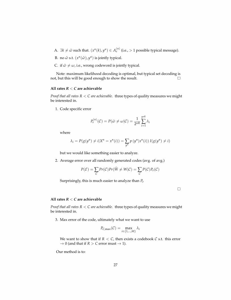
Proof that all rates R < C are achievable. three types of quality measures we mightbe interested in.
1. Code specific error
P(n)e (C) = P(ω 6= ω|C) = 1
2nR
2nR
∑i=1
λi
where
λi = P(g(yn) 6= i|Xn = xn(i)) = ∑yn
p (yn|xn(i)) I(g(yn) 6= i)
but we would like something easier to analyze.
2. Average error over all randomly generated codes (avg. of avg.)
P(E) = ∑C
Pr(C)Pr(W 6= W|C) = ∑C
P(C)Pe(C)
Surprisingly, this is much easier to analyze than Pe
All rates R < C are achievable
Proof that all rates R < C are achievable. three types of quality measures we mightbe interested in.
3. Max error of the code, ultimately what we want to use
PC,max(C) = maxi∈{1,...,M}
λi
We want to show that if R < C, then exists a codebook C s.t. this error→ 0 (and that if R > C error must→ 1).
Our method is to:
27

1. Expand average error (bullet 2 above) and show that it is small.
2. deduce that ∃ at least one code with small error
3. show that this can be modified to have small maximum probability oferror.
All rates R < C are achievable
Proof that all rates R < C are achievable.
P(E) = ∑C
P(C)P(n)e (C) = ∑
CP(C) 1
2nR
2nR
∑ω=1
λω (C) (24)
=1
2nR
2nR
∑ω=1
∑C
P(C)λω (C) (25)
but
∑C
P(C)λw (C) = ∑C
P (g (Yn) 6= ω|Xn = xn(ω))
∏2nRi=1 P(xn(i))︷ ︸︸ ︷
P(
xn(1), . . . , xn(
2nR))
︸ ︷︷ ︸T
= ∑xn(1),...,xn(2nR)
T
All rates R < C are achievable
Proof that all rates R < C are achievable.
P(C)λω(C)= ∑ ∏
i 6=ω
P(xn(i))︸ ︷︷ ︸1
∑xn(ω)
P (g (Yn) 6= ω|Xn = xn(ω)) P (xn(ω))
= ∑xn(ω)
P (g (Yn) 6= ω|Xn = xn(ω)) P (xn(ω))
= ∑xn(ω)
P (g (Yn) 6= 1|Xn = xn(1)) P (xn(1)) = ∑C
P(C)λ1 (C) = β
Last sum is the same regardless of ω, call it β. Thus, we can can arbitrarilyassume that ω = 1.
28
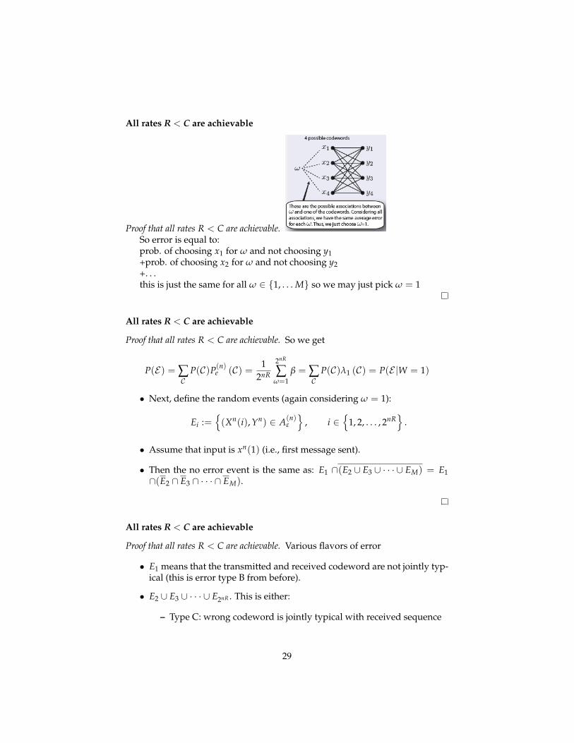
All rates R < C are achievable
Proof that all rates R < C are achievable.So error is equal to:prob. of choosing x1 for ω and not choosing y1+prob. of choosing x2 for ω and not choosing y2+. . .this is just the same for all ω ∈ {1, . . . M} so we may just pick ω = 1
All rates R < C are achievable
Proof that all rates R < C are achievable. So we get
P(E) = ∑C
P(C)P(n)e (C) = 1
2nR
2nR
∑ω=1
β = ∑C
P(C)λ1 (C) = P(E|W = 1)
• Next, define the random events (again considering ω = 1):
Ei :={(Xn(i), Yn) ∈ A(n)
ε
}, i ∈
{1, 2, . . . , 2nR
}.
• Assume that input is xn(1) (i.e., first message sent).
• Then the no error event is the same as: E1 ∩(E2 ∪ E3 ∪ · · · ∪ EM) = E1∩(E2 ∩ E3 ∩ · · · ∩ EM).
All rates R < C are achievable
Proof that all rates R < C are achievable. Various flavors of error
• E1 means that the transmitted and received codeword are not jointly typ-ical (this is error type B from before).
• E2 ∪ E3 ∪ · · · ∪ E2nR . This is either:
– Type C: wrong codeword is jointly typical with received sequence
29

– Type A: greater than 1 codeword is jointly typical with received se-quence
so this is type C and A both.Our goal is to bound the probability of error, but lets look at some figures
first.
All rates R < C are achievable
Proof that all rates R < C are achievable.
All rates R < C are achievable
Proof that all rates R < C are achievable.
30

All rates R < C are achievable
Proof that all rates R < C are achievable.
All rates R < C are achievable
Proof that all rates R < C are achievable. Goal: bound the probability of error:
P(E|W = 1) = P(E1 ∪ E2 ∪ E3 ∪ . . .
)≤ P
(E1)+
2nR
∑i=2
P(Ei)
We have that
P(E1)= P
(A(n)
ε
)→ 0 (n→ ∞)
So, ∀ε > 0∃n0 such thatP(E1)≤ ε, ∀n > n0
All rates R < C are achievable
Proof that all rates R < C are achievable. • Also, because of random code gen-eration process (and recall, ω = 1), Xn(1) and Xn(i) i.r.v., hence Xn(i) andYn i.r.v for i 6= 1
• This gives, for i 6= 1,
P
(Xn(i), Yn) ∈ A(n)ε︸ ︷︷ ︸
indep. events
≤ 2−n(I(X;Y)−3ε)
by the joint AEP.
31

• This will allow us to bound the error, as long as I(X; Y) > 3ε.
All rates R < C are achievable
Proof that all rates R < C are achievable. Consequently,
P(E) = P(E|W = 1) ≤ P(E1|W = 1
)+
2nR
∑i=2
P(Ei|W = 1)
≤ ε +2nR
∑i=2
2−n(I(X;Y)−3ε)
= ε +(
2nR − 1)
2−n(I(X;Y)−3ε)
≤ ε + 23nε2−n(I(X;Y)−R)
= ε + 2−n[(I(X;Y)−3ε)−R]
≤ 2ε
The last statement is true only if I(X; Y)− 3 > R.
All rates R < C are achievable
Proof that all rates R < C are achievable. • So if we chose R < I(X; Y) (strictly),we can find an ε and n so that the average probability of error P(E) ≤ 2ε,can be made as small as we want.
• But, we need to get from an average to a max probability of error, andbound that.
• First, choose p(x) = argmaxp(x) I(X; Y) rather than uniform p(x), to changethe condition from R < I(X; Y) to R < C. Thus, this gives us higher ratelimit.
• If P(E) ≤ 2ε, the bound on the average error is small, so there must existsome specific code, say C∗ s.t.
P(n)e (C∗) ≤ 2ε.
All rates R < C are achievable
32

Proof that all rates R < C are achievable. • Lets break apart this error proba-bility.
P(n)e (C∗) = 1
2nR
2nR
∑i=1
λi (C∗)
=1
2nR ∑i:λi<4ε
λi (C∗) +1
2nR ∑i:λi≥4ε
λi (C∗)
• Now suppose more than half of the indices had error ≥ 4ε (i.e., suppose|{i : λi ≥ 4ε}| ≥ 2nR/2 = 2nR−1). Under this assumption
12nR ∑
i:λi≥4ε
λi (C∗) ≥1
2nR ∑i:λi≥4ε
4ε =1
2nR |{i : λi ≥ 4ε}| 4ε > 2ε.
All rates R < C are achievable
Proof that all rates R < C are achievable. • Can’t be since these alone wouldbe more than our 2ε upper bound.
• Hence, at most half the codewords can have error ≥ 4ε , and we get
|{i : λi ≥ 4ε}| ≥ 2nR/2 =⇒ |{i : λi < 4ε}| ≥ 2nR/2
• Create a new codebook that eliminates all bad codewords (i.e., those inwith index {i : λi ≥ 4ε}). There are at most half of them.
• The remaining codewords are of size ≥ 2nR/2 = 2nR−1 = 2n(R−1/n)(atleast half of them). They all have max probability ≤ 4ε .
• We now code with rate R′ = R− 1/n → R as n → ∞, but for this newsequence of codes, the max error probability (n) 4 , which can be made assmall as we wish.
Discussion
• To summarize, random coding is the method of proof to show that ifR < C, there exists a sequence of (2nR, n) codes with λ(n) → 0 as n→ ∞.
• This might not be the best code, but it is sufficient. It is an existence proof.
• Huge literature on coding theory. We’ll discuss Hamming codes.
• But many good codes exist today: Turbo codes, Gallager (or low-density-parity-check) codes, and new ones are being proposed often.
33

• But we have yet to prove the converse . . .
• We next need to show that any sequence of (2nR, n) codes with (2nR, n)must have that R < C.
• First lets consider the case if P(n)e = 0, in such case it is easy to show that
R < C.
6.2 Zero-Error Codes
Zero-Error Codes
• P(n)e = 0 =⇒ H(W|Yn) = 0 (no uncertainty)
• For the sake of an easy proof, assume H(W) = nR = log M (i.e., uniformdistribution over {1, 2, . . . , M}.
• First lets consider the case if P(n)e = 0, in such case it is easy to show that
R < C. Then we get
nR = H(W) = H(W|Yn) + I(W; Yn) = I(W; Yn)
≤ I(Xn; Yn) // Since W → Xn → Yn Markov chain and DP inequality
≤n
∑i=1
I(Xi; Yi) //Fano’s lemma, follows next
≤ nC //definition of capacity
• HenceR ≤ C.
6.3 Fano’s Lemmas
Fano’s Lemmas
Lemma 23. For a DMC with a codebook C and the input message W uniformlydistributed over 2nR
H(W|W) ≤ 1 + P(n)e nR (26)
Proof. W uniformly distributed =⇒ P(n)e = P(W 6= W). We apply Fano’s in-
equality1 + Pe log |X | ≥ H(X|Y);
for W and an alphabet of length 2nR.
Next lemma shows that the capacity per transmission is not increased if weuse a DMC many times.
34

Lemma 24. Let Yn be the result of passing Xn through a memoryless channel ofcapacity C. Then
I (Xn; Yn) ≤ nC, ∀p(xn). (27)
Proof.
I (Xn; Yn) = H (Yn)− H (Yn|Xn)
= H (Yn)−n
∑i=1
H(Yi|Y1, . . . , Yi−1, Xn)
= H (Yn)−n
∑i=1
H(Yi|Xi) //def. of DMC
Fano’s Lemmas
Proof - continuation.
I (Xn; Yn) = H (Yn)−n
∑i=1
H(Yi|Xi)
≤n
∑i=1
H(Yi)−n
∑i=1
H(Yi|Xi)
=n
∑i=1
I(Xi; Yi)︸ ︷︷ ︸≤C
≤ nC.
6.4 Converse to the Channel Coding Theorem
Converse to the Channel Coding TheoremThe converse states: any sequence of (2nR; n) codes with λ(n) → 0 must
have that R < C.
Proof that λ(n) → 0 as n→ ∞⇒ R < C. • Average prob. goes to zero if maxprobability does: λ(n) → 0⇒ P(n)
e → 0, where P(n)e = 1
2nR ∑2nR
i=1 λi
• Set H(W) = nR for now (i.e., W uniform on{
1, 2, . . . , M = 2nR}). Again,makes the proof a bit easier and
• doesn’t affect relationship between R and C).
• So, P(
W 6= W)= P(n)
e = 1M ∑M
i=1 λi
35

Converse to the Channel Coding Theorem
Proof that λ(n) → 0 as n→ ∞⇒ R < C.
nR = H(W) = H(
W|W)+ I
(W; W
)//uniformity of W
≤ 1 + P(n)e nR + I
(W; W
)//by Fano’s Lemma 23
≤ 1 + P(n)e nR + I (Xn; Yn) //DP inequality
≤ 1 + P(n)e nR + nC //Lemma 24
R ≤ P(n)e R + C +
1n
(28)
Now as n→ ∞, P(n)e → 0, and 1/n→ 0 as well. Thus R < C.
Proof that λ(n) → 0 as n→ ∞⇒ R < C.
• We rewrite (28) as
P(n)e ≥ 1− C
R− 1
nR.
• if n → ∞ and R > C, then error lower bound is strictly positive, anddepends on 1− C/R.
• Even for small n, P(n)e > 0, since otherwise, if P(n0)
e = 0 for some code, wecan concatenate code to get large n same rate code, contradicting Pe > 0.
• Hence we cannot achieve an arbitrarily low probability of error at ratesabove capacity
• This coverse is called weak converse
• strong converse: if R > C, P(n)e → 1
6.5 Equality in the Converse to the Channel Coding Theorem
Equality in the Converse to the Channel Coding TheoremWhat if we insist on R = C and Pe = 0. In such case, what are the require-
36

ments of any such code.
nR = H(W) = H(Xn(W))
= H(W|W)︸ ︷︷ ︸=0, since Pe=0
+I(W; W) = I(W; W)
= H(Yn)− H(Yn|Xn)
= H(Yn)−n
∑i=1
(Yn|Xi)
= ∑i
H(Yi)−∑i
H(Yi|Xi) //if all Yi indep.
= ∑i
I (Xi; Yi)
= nC //p∗(x) ∈ arg maxp(x)
I(Xi; Yi)
So there are 3 conditions for equality, R = C, namely
1. all codewords must be distinct
2. Yi’s are independent
3. distribution on x is p∗(x), a capacity achieving distribution.
7 Feedback Capacity
Feedback CapacityConsider a sequence of channel uses.
37

Another way of looking at it is:
Can this help, i.e., can this increase C?
Does feedback help for DMC
• A: No.
• Intuition: w/o memory, feedback tells us nothing more than what wealready know, namely p(y|x).
• Can feedback made decoding easier? Yes, consider binary erasure chan-nel, when we get Y = e we just re-transmit.
• Can feedback help for channels with memory? In general, yes.
Feedback for DMC
Definition 25. A (2nR, n) feedback code is is the encoder Xi(W; Y1:i−1), a de-coder g : Yn →
{1, 2, . . . , 2nR} and P(n)
e = P (g (Yn) 6= W), for H(W) = nR(uniform).
Definition 26 (Capacity with feedback). The capacity with feedback CFB of aDMC is the supremum of all rates achievable by feedback codes.
Theorem 27 (Feedback capacity).
CFB = C = maxp(x)
I(X; Y). (29)
Feedback codes for DMC
Proof. • Clearly,CFB > C, since FB code is a generalization.
• Next, we use W instead of X and bound R.
• We have
H(W) = H(W|W) + I(W; W)
≤ 1 + P(n)e nR + I(W; W) //by Fano
≤ 1 + P(n)e nR + I(W; Yn) //DP ineq.
• We next bound I(W; Yn)
38

Feedback codes for DMC
. . . proof continued.
I(W; Yn) = H(Yn)− H(Yn|W) = H(Yn)−n
∑i=1
H (Yi|Y1:i−1, W)
= H(Yn)−n
∑i=1
H (Yi|Y1:i−1, W, Xi) //Xi = f (W, Y1:i−1)
= H(Yn)−n
∑i=1
H (Yi|Xi) ≤∑i[H(Yi)− H (Yi|Xi)]
= ∑i
I(Xi; Yi) ≤ nC
Feedback codes for DMC
. . . proof continued. Thus we have
nR = H(W) ≤ 1 + P(n)e nR + nC
=⇒ R ≤ 1n+ P(n)
e R + C =⇒ R ≤ C < CFB.
Thus, feedback does not help.
8 Source-Channel Separation Theorem
Joint Source/Channel Theorem
• Data compression: We now know that it is possible to achieve error freecompression if our average rate of compression, R, measured in units ofbits per source symbol, is such that R > H where H is the entropy of thegenerating source distribution.
• Data Transmission: We now know that it is possible to achieve error freecommunication and transmission of information if R < C, where R is theaverage rate of information sent (units of bits per channel use), and C isthe capacity of the channel.
• Q: Does this mean that if H < C, we can reliably send a source of entropyH over a channel of capacity C?
• This seems intuitively reasonable.
39

Joint Source/Channel Theorem: processThe process would go something as follows:
1. Compress a source down to its entropy, using Huffman, LZ, arithmeticcoding, etc.
2. Transmit it over a channel.
3. If all sources could share the same channel, would be very useful.
4. I.e., perhaps the same channel coding scheme could be used regardlessof the source, if the source is first compressed down to the entropy. Thechannel encoder/decoder need not know anything about the originalsource (or how to encode it).
5. Joint source/channel decoding as in the following figure:
6. Maybe obvious now, but at the time (1940s) it was a revolutionary idea!
Source/Channel Separation Theorem
• Source: V ∈ V that satisfies AEP (e.g., stationary ergodic).
• Send V1:n = V1, V2, . . . , Vn over channel, entropy rate H(V) of stochasticprocess (if i.i.d., H(V) = H(Vi), ∀i).
• Error probability and setup:
P(n)e = P
(V1:n 6= V1:n
)= ∑
y1:n∑v1:n
P(v1:n)P (y1:n|Xn(v1:n)) I {g (y1:n) 6= v1:n}
where I indicator function, g decoding function
40

Source/Channel Coding Theorem
Theorem 28 (Source-channel coding theorem). If V1:n satisfies AEP and if H(V) <C, then ∃ a sequence of (2nR; n) codes with P(n)
e → 0. Conversely, if H(V) > C, thenP(n)
e > 0 for all n and cannot send the process with arbitrarily low probability of error.
Proof. • If V satisfies AEP, then ∃ a set A(n)ε with
∣∣∣A(n)ε
∣∣∣ < 2n(H(V)+ε) (A(n)ε
has all the probability).
• We only encode the typical set, and signal an error otherwise. This εcontributes to Pe.
• We index elements of A(n)ε as
{1, 2, . . . , 2n(H+ε)
}, so need n(H + ε) bits.
• This gives a rate of R = H(V) + ε. If R < C then the error < ε, which wecan make as small as we wish.
Source/Channel Coding Theorem
. . . proof continued. • Then
P(n)e = P(V1:n 6= V1:n)
≤ P(V1:n /∈ A(n)ε ) +P
(g (Yn) 6= Vn|Vn ∈ A(n)
ε
)︸ ︷︷ ︸
<ε, since R<C
≤ ε + ε = 2ε,
• and the first part of the theorem is proved.
• To show the converse, show that P(n)e → 0 ⇒ H(V) < C for source
channel codes.
Source/Channel Coding Theorem
. . . proof continued. • Define:
Xn(Vn) : Vn → X n //encodergn (Yn) : X n → Vn //decoder
• Now recall, original Fano says H(X|Y) ≤ 1 + Pe log |X |.
• Here we have
H(Vn|Vn) ≤ 1 + P(n)e log |Vn| = 1 + nPe log |X |
41

Source/Channel Coding Theorem
. . . proof continued. • We get the following derivation
H(V) ≤ H(V1, V2, . . . , Vn)
n=
H(V1:n)
n
=1n
H(V1:n|V1:n) +1n
I(V1:n; V1:n)
≤ 1n
(1 + P(n)
e log |Vn|)+
1n
I(V1:n; V1:n) //by Fano
≤ 1n
(1 + P(n)
e log |Vn|)+
1n
I(X1:n; Y1:n) //V → X → Y → V
≤ 1n+ P(n)
e log |V|+ C //memoryless
• Letting n→ ∞, 1/n and Pe → 0 which leaves us with H(V) ≤ C.
9 Coding
9.1 Introduction to coding
Coding and codes
• Shannon’s theorem says that there exists a sequence of codes such that ifR < C the error goes to zero.
• It doesn’t provide such a code, nor does it offer much insight on how tofind one.
• Typical set coding is not practical. Why? Exponentially large sized blocks.
• In all cases, we add enough redundancy to a message so that the originalmessage can be decoded unambiguously
Physical Solution to Improve Coding
• It is possible to communicate more reliably by changing physical proper-ties to decrease the noise (e.g., decrease p in a BSC).
• Use more reliable and expensive circuitry
• improve environment (e.g., control thermal conditions, remove dust par-ticles or even air molecules)
• In compression, use more physical area/volume for each bit.
• In communication, use higher power transmitter, use more energy therebymaking noise less of a problem.
• These are not IT solutions which is what we want.
42

Repetition Repetition Repetition Code Code Code
• Rather than send message x1x2 . . . xk we repeat each symbol K times re-dundantly.
• Recall our example of repeating each word in a noisy analog radio con-nection.
• Message becomes x1x1 . . . x1︸ ︷︷ ︸K×
x2x2 . . . x2︸ ︷︷ ︸K×
. . .
• For many channels (e.g., BSC(p < 1/2)), error goes to zero as k→ 1.
• Easy decoding: when K is odd, take a majority vote (which is optimal fora BSC)
• On the other hand, Rα1/K → 0 as K → ∞
• This is really a pre-1948 way of thinking code.
• Thus, this is not a good code.
Repetition Code Example
• (From D. Mackay [2]) Consider sending message s = 0010110
• One scenarios 0 0 1 0 1 1 0
t︷︸︸︷000
︷︸︸︷000
︷︸︸︷111
︷︸︸︷000
︷︸︸︷111
︷︸︸︷111
︷︸︸︷000
n 000 001 000 000 101 000 000r 000 001 111 000 010 111 000
• Another scenarios 0 0 1 0 1 1 0
t︷︸︸︷000
︷︸︸︷000
︷︸︸︷111
︷︸︸︷000
︷︸︸︷111
︷︸︸︷111
︷︸︸︷000
n 000 001 000 000 101 000 000r 000︸︷︷︸ 001︸︷︷︸ 111︸︷︷︸ 000︸︷︷︸ 010︸︷︷︸ 111︸︷︷︸ 000︸︷︷︸s 0 0 1 0 0 1 0corrected errors *undetected errors *
• Thus, can only correct one bit error not two.
Simple Parity Check Code
• Binary input/output alphabets X = Y = {0, 1}.
• Block sizes of n− 1 bits: x1:n−1.
43

• nth bit is an indicator of an odd number of 1 bits in.
• I.e., xn ← mod(
∑n−1i=1 xi, 2
)• Thus a necessary condition for valid code word is: mod
(∑n−1
i=1 xi, 2)= 0.
• Any any instance of an odd number of errors (bit swaps) won’t pass thiscondition (although an even number of errors will pass the condition).
• Quite perfect: can not correct errors, and moreover only detects some ofthe kinds of errors (odd number of swaps).
• On the other hand, parity checks form the basis for many sophisticatedcoding schemes (e.g., low-density parity check (LDPC) codes, Hammingcodes etc.).
• We study Hamming codes next.
9.2 Hamming Codes
(7; 4; 3) Hamming Codes
• Best illustrated by an example.
• Let X = Y = {0, 1}.
• Fix the desired rate at R = 4/7 bit per channel use.
• Thus, in order to send 4 data bits, we need to use the channel 7 times.
• Let the four data bits be denoted x0, x1, x2, x3 ∈ {0, 1}.
• When we send these 4 bits, we are also going to send 3 additional parityor redundancy bits, named x4, x5, x6.
• Note: all arithmetic in the following will be mod 2, i.e. 1 + 1 = 0, 1 + 0 =1, 1 = 0− 1 = −1, etc.
• Parity bits determined by the following equations:
x4 ≡ x1 + x2 + x3 mod 2x5 ≡ x0 + x2 + x3 mod 2x6 ≡ x0 + x1 + x3 mod 2
• I.e., if (x0, x1, x2, x3) = (0110) then (x4, x5, x6) = (011) and complete 7-bitcodeword sent over channel would be (0110011).
44

• We can also describe this using linear equalities as follows (all mod 2).
x1 +x2 +x3 +x4 = 0x0 +x2 +x3 +x5 = 0x0 +x1 +x3 +x6 = 0
• Or alternatively, as Hx = 0 where xT = (x1, x2, . . . , x7) and
H =
0 1 1 1 1 0 01 0 1 1 0 1 01 1 0 1 0 0 1
• Notice that H is a column permutation of all non-zero length-3 column
vectors.
• H is called parity-check matrix
• Thus the code words are defined by the null-space of H, i.e., {x : Hx =0}.
• Since the rank of H is 3, the null-space dimension is 4, and we expectthere to be 16 = 24 binary vectors in this null space.
• These 16 vectors are:
0000000 0100101 1000011 10000110001111 0101010 1001100 10011000010110 0110011 1010101 10101010011001 0111100 1011010 1011010
Hamming Codes : weight
• Thus, any codeword is in C = {x : Hx = 0}.
• Thus, if v1, v2 ∈ C then v1 + v2 ∈ C and v1 − v2 ∈ C due to linearity(codewords closed under addition and subtraction).
• weight of a code is 3, which is minimum number of ones in any non-zerocodeword.
• Why? Since columns of H are all different, sum of any two columns isnon-zero, so can’t have any weight-2v (summing two columns is neverzero).
• Minimum weight is 3 since sum of two columns will equal another col-umn, and sum of two equal column vectors is zero.
45

Hamming Codes : Distance
• Thus, any codeword is in C = {x : Hx = 0}.
• minimum distance of a code is also 3, which is minimum number of dif-ferences between any two codewords.
• Why? Given v1, v2 ∈ C⇒ (v1 − v2) ∈ C. Can’t have difference (or sum,and 1+1 = 1-1) of any two columns equaling zero, so v1 − v2 can’t differin only two places.
• Another way of saying this: if v1, v2 ∈ C then dH(v1, v2) ≥ 3 wheredH(·, ·) is the Hamming distance.
• In general, codes with large minimum distance is good because then it ispossible to correct errors, i.e., if v is received codeword, then we can findi ∈ argminidH(v, vi) as the decoding procedure.
Hamming Codes : BSC
• Now a BSC(p) (crossover probability p) will chance some of the bits (noise),meaning a 0 might change to a 1 and vice verse.
• So if x = (x0, x1, . . . , x6) is transmitted, what is received is y = x + z =(x0 + z0; x1 + z1, . . . , x6 + z6), where z = (z0, z1, . . . , z6) is the noise vector.
• Receiver knows y but wants to know x. We then compute
s = Hy = H(x + z) = Hx︸︷︷︸=0
+Hz = Hz
• s is called the syndrome of y. s = 0 means that all parity checks aresatisfied by y and is a necessary condition for a correct codeword.
• Moreover, we see that s is a linear combination of columns of H
s = z0
011
+ z1
101
+ z2
110
+ · · ·+ z6
001
• Since y = x + z, we know y, so if we know z we know x.
• We only need to solve for z in s = Hz, 16 possible solutions.
• Ex: Suppose that yT = 0111001 is received, then sT = (101) and the 16solutions are:
0100000 0010011 0101111 10010011100011 0001010 1000110 11110100000101 0111001 1110101 00111000110110 1010000 1101100 1011111
46
• 16 is better than 128 (possible z vectors) but still many.
• What is the probability of each solution? Since we are assuming a BSC(p)with p < 1/2, the most probable solution has the leastweight. Any solu-tion with weight k has probability pk.
• Notice that there is only one possible solution with weight 1, and this ismost probable solution.
• In previous example, most probable solution is zT = (01000000) and iny = x + z with yT = 0111001 this leads to codeword x = 0011001 andinformation bits 0011.
• In fact, for any s, there is a unique minimum weight solution for z ins = Hz (in fact, this weight is no more than 1)!
• If s = (000) then the unique solution is z = (0000000).
• For any other s, then s must be equal to one of the columns of H, so wecan generate s by flipping the corresponding bit of z on (giving weight 1solution).
Hamming Decoding ProcedureHere is the final decoding procedure on receiving y:
1. Compute the syndrome s = Hy.
2. If s = (000) set z← (0000000) and goto 4.
3. Otherwise, locate unique column of H equal to s form z all zeros but witha 1 in that position.
4. Set x ← y + z.
5. output (x0, x1, x2, x3) as the decoded string.
This procedure can correct any single bit error, but fails when there is morethan one error.
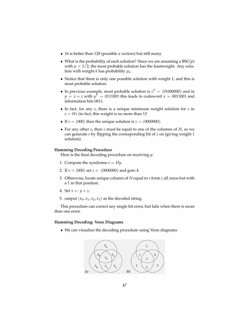
Hamming Decoding: Venn Diagrams
• We can visualize the decoding procedure using Venn diagrams
47

• Here, first four bits to be sent (x0, x1, x2, x3) are set as desired and paritybits (x4, x5, x6) are also set. Figure shows (x0; x1, . . . , x6) = (1, 0, 0, 0, 1, 0, 1)with parity check bits:
x4 ≡ x0 + x1 + x2 mod 2x5 ≡ x1 + x2 + x3 mod 2x6 ≡ x0 + x2 + x3 mod 2
Hamming Decoding: Venn Diagrams
• The syndrome can be seen as a condition where the parity conditions arenot satisfied.
• Above we argued that for s 6= (0, 0, 0) there is always a one bit flip thatwill satisfy all parity conditions.
Hamming Decoding: Venn Diagrams
• Example: Here, z1 can be flipped to achieve parity.
48

Hamming Decoding: Venn Diagrams
• Example: Here, z4 can be flipped to achieve parity.
Hamming Decoding: Venn Diagrams
• Example: And here, z2 can be flipped to achieve parity.
Hamming Decoding: Venn Diagrams
• Example: And here, there are two errors, y6 and y2 (marked with a *).
• Flipping y1 will achieve parity, but this will lead to three errors (i.e., wewill switch to a wrong codeword, and since codewords have minimumHamming distance of 3, we’ll get 3 bit errors).
49

Coding
• Many other coding algorithms.
• Reed Solomon Codes (used by CD players).
• Bose, Ray-Chaudhuri, Hocquenghem (BCH) codes.
• Convolutional codes
• Turbo codes (two convolutional codes with permutation network)
• Low Density Parity Check (LDPC) codes.
• All developed on our journey to find good codes with low rate that achieveShannon’s promise.
References
References
[1] Thomas M. Cover, Joy A. Thomas, Elements of Information Theory, 2nd edi-tion, Wiley, 2006.
[2] David J.C. MacKay, Information Theory, Inference, and Learning Algorithms,Cambridge University Press, 2003.
[3] Robert M. Gray, Entropy and Information Theory, Springer, 2009
50

References
[1] D. A. Huffman, A method for the construction of minimum redundancycodes, Proc. IRE, 40: 1098–1101,1952
[2] C. E. Shannon, A mathematical theory of communication, Bell SystemTechnical Journal, 1948.
[3] R. V. Hamming, Error detecting and error correcting codes, Bell SystemTechnical Journal, 29: 147-160, 1950
51