Chaos: A Very Short Introduction

Very Short Introductions are for anyone wanting a stimulating

and accessible way in to a new subject. They are written by experts, and have

been published in more than 25 languages worldwide.

The series began in 1995, and now represents a wide variety of topics

in history, philosophy, religion, science, and the humanities. Over the next

few years it will grow to a library of around 200 volumes – a Very Short

Introduction to everything from ancient Egypt and Indian philosophy to

conceptual art and cosmology.

Very Short Introductions available now:

ANARCHISM Colin Ward

ANCIENT EGYPT Ian Shaw

ANCIENT PHILOSOPHY

Julia Annas

ANCIENT WARFARE

Harry Sidebottom

ANGLICANISM Mark Chapman

THE ANGLO-SAXON AGE

John Blair

ANIMAL RIGHTS David DeGrazia

ARCHAEOLOGY Paul Bahn

ARCHITECTURE

Andrew Ballantyne

ARISTOTLE Jonathan Barnes

ART HISTORY Dana Arnold

ART THEORY Cynthia Freeland

THE HISTORY OF

ASTRONOMY Michael Hoskin

Atheism Julian Baggini

Augustine Henry Chadwick

BARTHES Jonathan Culler

THE BIBLE John Riches

THE BRAIN Michael O’Shea

BRITISH POLITICS

Anthony Wright

Buddha Michael Carrithers

BUDDHISM Damien Keown

BUDDHIST ETHICS

Damien Keown

CAPITALISM James Fulcher

THE CELTS Barry Cunliffe

CHAOS Leonard Smith

CHOICE THEORY

Michael Allingham

CHRISTIAN ART Beth Williamson

CHRISTIANITY Linda Woodhead

CLASSICS Mary Beard and

John Henderson

CLAUSEWITZ Michael Howard

THE COLD WAR Robert McMahon

CONSCIOUSNESS Susan Blackmore

CONTEMPORARY ART

Julian Stallabrass

Continental Philosophy

Simon Critchley

COSMOLOGY Peter Coles

THE CRUSADES

Christopher Tyerman

CRYPTOGRAPHY

Fred Piper and Sean Murphy

DADA AND SURREALISM

David Hopkins

Darwin Jonathan Howard

THE DEAD SEA SCROLLS

Timothy Lim

Democracy Bernard Crick

DESCARTES Tom Sorell

DESIGN John Heskett

DINOSAURS David Norman

DREAMING J. Allan Hobson

DRUGS Leslie Iversen

THE EARTH Martin Redfern

ECONOMICS Partha Dasgupta

EGYPTIAN MYTH Geraldine Pinch

EIGHTEENTH-CENTURY

BRITAIN Paul Langford

THE ELEMENTS Philip Ball

EMOTION Dylan Evans

EMPIRE Stephen Howe

ENGELS Terrell Carver

Ethics Simon Blackburn

The European Union

John Pinder

EVOLUTION

Brian and Deborah Charlesworth

EXISTENTIALISM Thomas Flynn

FASCISM Kevin Passmore

FEMINISM Margaret Walters

THE FIRST WORLD WAR

Michael Howard

FOSSILS Keith Thomson

FOUCAULT Gary Gutting

THE FRENCH REVOLUTION

William Doyle

FREE WILL Thomas Pink

Freud Anthony Storr

FUNDAMENTALISM

Malise Ruthven

Galileo Stillman Drake

Gandhi Bhikhu Parekh

GLOBAL CATASTROPHES

Bill McGuire

GLOBALIZATION Manfred Steger

GLOBAL WARMING Mark Maslin

HABERMAS

James Gordon Finlayson

HEGEL Peter Singer

HEIDEGGER Michael Inwood

HIEROGLYPHS Penelope Wilson

HINDUISM Kim Knott

HISTORY John H. Arnold

HOBBES Richard Tuck

HUMAN EVOLUTION

Bernard Wood

HUME A. J. Ayer

IDEOLOGY Michael Freeden

Indian Philosophy

Sue Hamilton

Intelligence Ian J. Deary

INTERNATIONAL

MIGRATION Khalid Koser

ISLAM Malise Ruthven

JOURNALISM Ian Hargreaves

JUDAISM Norman Solomon

Jung Anthony Stevens

KAFKA Ritchie Robertson

KANT Roger Scruton

KIERKEGAARD Patrick Gardiner

THE KORAN Michael Cook

LINGUISTICS Peter Matthews

LITERARY THEORY

Jonathan Culler

LOCKE John Dunn

LOGIC Graham Priest

MACHIAVELLI Quentin Skinner

THE MARQUIS DE SADE

John Phillips

MARX Peter Singer

MATHEMATICS Timothy Gowers

MEDICAL ETHICS Tony Hope

MEDIEVAL BRITAIN

John Gillingham and

Ralph A. Griffiths

MODERN ART David Cottington

MODERN IRELAND

Senia Paseta

MOLECULES Philip Ball

MUSIC Nicholas Cook

Myth Robert A. Segal

NATIONALISM Steven Grosby

NEWTON Robert Iliffe

NIETZSCHE Michael Tanner

NINETEENTH-CENTURY

BRITAIN Christopher Harvie and

H. C. G. Matthew

NORTHERN IRELAND

Marc Mulholland

PARTICLE PHYSICS Frank Close

paul E. P. Sanders

Philosophy Edward Craig

PHILOSOPHY OF LAW

Raymond Wacks

PHILOSOPHY OF SCIENCE

Samir Okasha

PHOTOGRAPHY Steve Edwards

PLATO Julia Annas

POLITICS Kenneth Minogue

POLITICAL PHILOSOPHY

David Miller

POSTCOLONIALISM

Robert Young

POSTMODERNISM

Christopher Butler

POSTSTRUCTURALISM

Catherine Belsey

PREHISTORY Chris Gosden

PRESOCRATIC PHILOSOPHY

Catherine Osborne

Psychology Gillian Butler and

Freda McManus

PSYCHIATRY Tom Burns

QUANTUM THEORY

John Polkinghorne

THE RENAISSANCE Jerry Brotton

RENAISSANCE ART

Geraldine A. Johnson

ROMAN BRITAIN Peter Salway

THE ROMAN EMPIRE

Christopher Kelly

ROUSSEAU Robert Wokler

RUSSELL A. C. Grayling

RUSSIAN LITERATURE

Catriona Kelly

THE RUSSIAN REVOLUTION

S. A. Smith

SCHIZOPHRENIA

Chris Frith and Eve Johnstone

SCHOPENHAUER

Christopher Janaway

SHAKESPEARE

Germaine Greer

SIKHISM Eleanor Nesbitt

SOCIAL AND CULTURAL

ANTHROPOLOGY

John Monaghan and Peter Just

SOCIALISM Michael Newman

SOCIOLOGY Steve Bruce

Socrates C. C. W. Taylor

THE SPANISH CIVIL WAR

Helen Graham

SPINOZA Roger Scruton

STUART BRITAIN

John Morrill

TERRORISM

Charles Townshend

THEOLOGY David F. Ford

THE HISTORY OF TIME

Leofranc Holford-Strevens

TRAGEDY Adrian Poole

THE TUDORS John Guy

TWENTIETH-CENTURY

BRITAIN Kenneth O. Morgan

THE VIKINGS Julian D. Richards

Wittgenstein A. C. Grayling

WORLD MUSIC Philip Bohlman

THE WORLD TRADE

ORGANIZATION

Amrita Narlikar

Available soon:

AFRICAN HISTORY

John Parker and

Richard Rathbone

CHILD DEVELOPMENT

Richard Griffin

CITIZENSHIP Richard Bellamy

HIV/AIDS Alan Whiteside

HUMAN RIGHTS

Andrew Clapham

INTERNATIONAL RELATIONS

Paul Wilkinson

RACISM Ali Rattansi

For more information visit our web site

www.oup.co.uk/general/vsi/

Leonard A. Smith

CHAOSA Very Short Introduction

1

3Great Clarendon Street, Oxford ox2 6dp

Oxford University Press is a department of the University of Oxford.It furthers the University’s objective of excellence in research, scholarship,

and education by publishing worldwide in

Oxford New York

Auckland Cape Town Dar es Salaam Hong Kong KarachiKuala Lumpur Madrid Melbourne Mexico City Nairobi

New Delhi Shanghai Taipei Toronto

With offices in

Argentina Austria Brazil Chile Czech Republic France GreeceGuatemala Hungary Italy Japan Poland Portugal SingaporeSouth Korea Switzerland Thailand Turkey Ukraine Vietnam

Oxford is a registered trade mark of Oxford University Pressin the UK and in certain other countries

Published in the United Statesby Oxford University Press Inc., New York

© Leonard A. Smith 2007

The moral rights of the author have been assertedDatabase right Oxford University Press (maker)

First published as a Very Short Introduction 2007

All rights reserved. No part of this publication may be reproduced,stored in a retrieval system, or transmitted, in any form or by any means,

without the prior permission in writing of Oxford University Press,or as expressly permitted by law, or under terms agreed with the appropriate

reprographics rights organizations. Enquiries concerning reproductionoutside the scope of the above should be sent to the Rights Department,

Oxford University Press, at the address above

You must not circulate this book in any other binding or coverand you must impose this same condition on any acquirer

British Library Cataloguing in Publication Data

Data available

Library of Congress Cataloging in Publication Data

Data available

Typeset by RefineCatch Ltd, Bungay, SuffolkPrinted in Great Britain by

Ashford Colour Press Ltd, Gosport, Hampshire

978–0–19–285378–3

1 3 5 7 9 10 8 6 4 2

To the memory of Dave Paul Debeer,

A real physicist, a true friend.

This page intentionally left blank

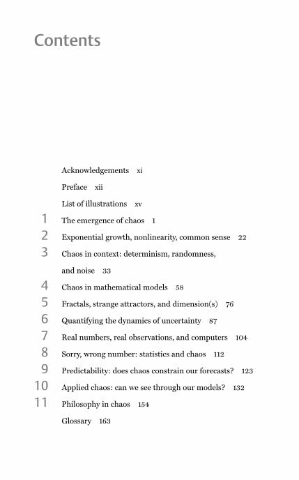
Contents

Acknowledgements xi

Preface xii

List of illustrations xv

1 The emergence of chaos 1

2 Exponential growth, nonlinearity, common sense 22

3 Chaos in context: determinism, randomness,

and noise 33

4 Chaos in mathematical models 58

5 Fractals, strange attractors, and dimension(s) 76

6 Quantifying the dynamics of uncertainty 87

7 Real numbers, real observations, and computers 104

8 Sorry, wrong number: statistics and chaos 112

9 Predictability: does chaos constrain our forecasts? 123

10 Applied chaos: can we see through our models? 132

11 Philosophy in chaos 154

Glossary 163

Further reading 169

Index 173

Acknowledgements

This book would not have been possible without my parents, of

course, but I owe a greater debt than most to their faith, doubt, and

hope, and to the love and patience of a, b, and c. Professionally my

greatest debt is to Ed Spiegel, a father of chaos and my thesis

Professor, mentor, and friend. I also profited immensely from

having the chance to discuss some of these ideas with Jim Berger,

Robert Bishop, David Broomhead, Neil Gordon, Julian Hunt,

Kevin Judd, Joe Keller, Ed Lorenz, Bob May, Michael Mackey,

Tim Palmer, Itamar Procaccia, Colin Sparrow, James Theiler,

John Wheeler, and Christine Ziehmann. I am happy to

acknowledge discussions with, and the support of, the Master

and Fellows of Pembroke College, Oxford. Lastly and largely, I’d

like to acknowledge my debt to my students, they know who they

are. I am never sure how to react upon overhearing an exchange

like: ‘Did you know she was Lenny’s student?’, ‘Oh, that explains

a lot.’ Sorry guys: blame Spiegel.

Preface

The ‘chaos’ introduced in the following pages reflects phenomena in

mathematics and the sciences, systems where (without cheating)

small differences in the way things are now have huge consequences

in the way things will be in the future. It would be cheating, of

course, if things just happened randomly, or if everything

continually exploded forever. This book traces out the remarkable

richness that follows from three simple constraints, which we’ll call

sensitivity, determinism, and recurrence. These constraints allow

mathematical chaos: behaviour that looks random, but is not

random. When allowed a bit of uncertainty, presumed to be the

active ingredient of forecasting, chaos has reignited a centuries-old

debate on the nature of the world.

The book is self-contained, defining these terms as they are

encountered. My aim is to show the what, where, and how of chaos;

sidestepping any topics of ‘why’ which require an advanced

mathematical background. Luckily, the description of chaos and

forecasting lends itself to a visual, geometric understanding; our

examination of chaos will take us to the coalface of predictability

without equations, revealing open questions of active scientific

research into the weather, climate, and other real-world

phenomena of interest.

Recent popular interest in the science of chaos has evolved

differently than did the explosion of interest in science a century

ago when special relativity hit a popular nerve that was to throb for

decades. Why was the public reaction to science’s embrace of

mathematical chaos different? Perhaps one distinction is that most

of us already knew that, sometimes, very small differences can have

huge effects. The concept now called ‘chaos’ has its origins both in

science fiction and in science fact. Indeed, these ideas were well

grounded in fiction before they were accepted as fact: perhaps the

public were already well versed in the implications of chaos, while

the scientists remained in denial? Great scientists and

mathematicians had sufficient courage and insight to foresee the

coming of chaos, but until recently mainstream science required a

good solution to be well behaved: fractal objects and chaotic curves

were considered not only deviant, but the sign of badly posed

questions. For a mathematician, few charges carry more shame

than the suggestion that one’s professional life has been spent on a

badly posed question. Some scientists still dislike problems whose

results are expected to be irreproducible even in theory. The

solutions that chaos requires have only become widely acceptable in

scientific circles recently, and the public enjoyed the ‘I told you so’

glee usually claimed by the ‘experts’. This also suggests why chaos,

while widely nurtured in mathematics and the sciences, took root

within applied sciences like meteorology and astronomy. The

applied sciences are driven by a desire to understand and predict

reality, a desire that overcame the niceties of whatever the formal

mathematics of the day. This required rare individuals who could

span the divide between our models of the world and the world as it

is without convoluting the two; who could distinguish the

mathematics from the reality and thereby extend the mathematics.

As in all Very Short Introductions, restrictions on space require

entire research programmes to be glossed over or omitted; I

present a few recurring themes in context, rather than a series of

shallow descriptions. My apologies to those whose work I have

omitted, and my thanks to Luciana O’Flaherty (my editor), Wendy

Parker, and Lyn Grove for help in distinguishing between what

was most interesting to me and what I might make interesting

to the reader.

How to read this introduction

While there is some mathematics in this book, there are no

equations more complicated than X = 2. Jargon is less easy to

discard. Words in bold italics you will have to come to grips with;

these are terms that are central to chaos, brief definitions of these

words can be found in the Glossary at the end of the book. Italics is

used both for emphasis and to signal jargon needed for the next

page or so, but which is unlikely to recur often throughout the book.

Any questions that haunt you would be welcome online at http://

cats.lse.ac.uk/forum/ on the discussion forum VSI Chaos. More

information on these terms can be found rapidly at Wikipedia

http://www.wikipedia.org/ and http://cats.lse.ac.uk/preditcability-

wiki/ , and in the Further reading.

List of illustrations

1 The first weather map

ever published in a

newspaper, prepared

by Galton in 1875 7© The Times/NI Syndication

Limited

2 Galton’s original sketch

of the Galton Board 9

3 The Times headline

following the Burns’

Day storm in 1990 13© The Times/NI Syndication

Limited 1990/John Frost

Newspapers

4 Modern weather map

showing the Burns’ Day

storm and a two-day-

ahead forecast 14

5 The Cheat with the Ace

of Diamonds, c.1645,

by Georges de la Tour 19Louvre, Paris. © Photo12.com/

Oronoz

6 A graph comparing

Fibonacci numbers and

exponential growth 26

7 A chaotic time series

from the Full Logistic

Map 39

8 Six mathematical

maps 40

9 Points collapsing onto

four attractors of the

Logistic Map 48

10 The evolution of

uncertainty under the

Yule Map 52

11 Period doubling

behaviour in the

Logistic Map 61

12 A variety of more

complicated behaviours

in the Logistic Map 62

13 Three-dimensional

bifurcation diagram and

the collapse toward

attractors in the

Logistic Map 63

14 The Lorenz attractor

and the Moore-Spiegel

attractor 67

15 The evolution of

uncertainty in the

Lorenz System 68

16 The Hénon attractor

and a two-dimensional

slice of the

Moore-Spiegel

attractor 70

17 A variety of behaviours

from the Hénon-Heilies

System 72

18 The Fournier Universe,

as illustrated by

Fournier 78

19 Time series from the

stochastic Middle Thirds

IFS Map and the

deterministic Tripling

Tent Map 82

20 A close look at the

Hénon attractor,

showing fractal

structure 84

21 Schematic diagrams

showing the action of

the Baker’s Map and a

Baker’s Apprentice

Map 98

22 Predictable chaos as

seen in four iterations

of the same mouse

ensemble under the

Baker’s Map and a

Baker’s Apprentice

Map 100

23 Card trick revealing the

limitations of digital

computers 108

24 Two views of data from

Machete’s electric circuit,

suggestive of Takens’

Theorem 118

25 The Not A Galton

Board 128

26 An illustration of using

analogues to make a

forecast 134

27 The state space of a

climate model 136Crown Copyright

28 Richardson’s dream 137© F. Schuiten

29 Two-day-ahead ECMWF

ensemble forecasts of the

Burns’ Day storm 140

30 Four ensemble forecasts

of the Machete’s Moore-

Spiegel Circuit 150

Figures 7, 8, 9, 11, 12, 13, 19, and 20 were produced with the

assistance of Hailiang Du. Figures 24 and 30 were produced with

the assistance of Reason Machete. Figures 4 and 29 were produced

with the assistance of Martin Leutbecher with data kindly made

available by the European Centre for Medium-Range Weather

Forecasting. Figure 27 is after M. Hume et al., The UKIP02

Scientific Report, Tyndal Centre, University of East Anglia,

Norwich, UK.

The publisher and the author apologize for any errors or omissions

in the above list. If contacted they will be pleased to rectify these at

the earliest opportunity.

This page intentionally left blank

Chapter 1

The emergence of chaos

Embedded in the mud, glistening green and gold and black,

was a butterfly, very beautiful and very dead.

It fell to the floor, an exquisite thing, a small thing

that could upset balances and knock down a line of

small dominoes and then big dominoes and then

gigantic dominoes, all down the years across Time.

Ray Bradbury (1952)

Three hallmarks of mathematical chaos

The ‘butterfly effect’ has become a popular slogan of chaos. But is it

really so surprising that minor details sometimes have major

impacts? Sometimes the proverbial minor detail is taken to be the

difference between a world with some butterfly and an alternative

universe that is exactly like the first, except that the butterfly is

absent; as a result of this small difference, the worlds soon come to

differ dramatically from one another. The mathematical version of

this concept is known as sensitive dependence. Chaotic systems

not only exhibit sensitive dependence, but two other properties as

well: they are deterministic, and they are nonlinear. In this

chapter, we’ll see what these words mean and how these concepts

came into science.

Chaos is important, in part, because it helps us to cope with

1

unstable systems by improving our ability to describe, to

understand, perhaps even to forecast them. Indeed, one of the

myths of chaos we will debunk is that chaos makes forecasting a

useless task. In an alternative but equally popular butterfly story,

there is one world where a butterfly flaps its wings and another

world where it does not. This small difference means a tornado

appears in only one of these two worlds, linking chaos to

uncertainty and prediction: in which world are we? Chaos is the

name given to the mechanism which allows such rapid growth of

uncertainty in our mathematical models. The image of chaos

amplifying uncertainty and confounding forecasts will be a

recurring theme throughout this Introduction.

Whispers of chaos

Warnings of chaos are everywhere, even in the nursery. The

warning that a kingdom could be lost for the want of a nail can be

traced back to the 14th century; the following version of the familiar

nursery rhyme was published in Poor Richard’s Almanack in 1758

by Benjamin Franklin:

For want of a nail the shoe was lost,

For want of a shoe the horse was lost,

and for want of a horse the rider was lost,

being overtaken and slain by the enemy,

all for the want of a horse-shoe nail.

We do not seek to explain the seed of instability with chaos, but

rather to describe the growth of uncertainty after the initial seed is

sown. In this case, explaining how it came to be that the rider was

lost due to a missing nail, not the fact that the nail had gone

missing. In fact, of course, there either was a nail or there was not.

But Poor Richard tells us that if the nail hadn’t been lost, then the

kingdom wouldn’t have been lost either. We will often explore the

properties of chaotic systems by considering the impact of slightly

different situations.

2

Ch

ao

s

The study of chaos is common in applied sciences like astronomy,

meteorology, population biology, and economics. Sciences making

accurate observations of the world along with quantitative

predictions have provided the main players in the development of

chaos since the time of Isaac Newton. According to Newton’s Laws,

the future of the solar system is completely determined by its

current state. The 19th-century scientist Pierre Laplace elevated

this determinism to a key place in science. A world is deterministic

if its current state completely defines its future. In 1820, Laplace

conjured up an entity now known as ‘Laplace’s demon’; in doing so,

he linked determinism and the ability to predict in principle to the

very notion of success in science.

We may regard the present state of the universe as the effect of its

past and the cause of its future. An intellect which at a certain

moment would know all forces that set nature in motion, and all

positions of all items of which nature is composed, if this intellect

were also vast enough to submit these data to analysis, it would

embrace in a single formula the movements of the greatest bodies of

the universe and those of the tiniest atom; for such an intellect

nothing would be uncertain and the future just like the past would

be present before its eyes.

Note that Laplace had the foresight to give his demon three

properties: exact knowledge of the Laws of Nature (‘all the forces’),

the ability to take a snapshot of the exact state of the universe (‘all

the positions’), and infinite computational resources (‘an intellect

vast enough to submit these data to analysis’). For Laplace’s

demon, chaos poses no barrier to prediction. Throughout this

Introduction, we will consider the impact of removing one or more

of these gifts.

From the time of Newton until the close of the 19th century, most

scientists were also meteorologists. Chaos and meteorology are

closely linked by the meteorologists’ interest in the role uncertainty

plays in weather forecasts. Benjamin Franklin’s interest in

3

Th

e e

me

rge

nce

of ch

ao

s

meteorology extended far beyond his famous experiment of flying

a kite in a thunderstorm. He is credited with noting the general

movement of the weather from west towards the east and testing

this theory by writing letters from Philadelphia to cities further

east. Although the letters took longer to arrive than the weather,

these are arguably early weather forecasts. Laplace himself

discovered the law describing the decrease of atmospheric pressure

with height. He also made fundamental contributions to the theory

of errors: when we make an observation, the measurement is never

exact in a mathematical sense, so there is always some uncertainty

as to the ‘True’ value. Scientists often say that any uncertainty in an

observation is due to noise, without really defining exactly

what the noise is, other than that which obscures our vision of

whatever we are trying to measure, be it the length of a table, the

number of rabbits in a garden, or the midday temperature.

Noise gives rise to observational uncertainty, chaos helps us to

understand how small uncertainties can become large

uncertainties, once we have a model for the noise. Some of the

insights gleaned from chaos lie in clarifying the role(s) noise

plays in the dynamics of uncertainty in the quantitative

sciences. Noise has become much more interesting, as the study

of chaos forces us to look again at what we might mean by the

concept of a ‘True’ value.

Twenty years after Laplace’s book on probability theory appeared,

Edgar Allan Poe provided an early reference to what we would now

call chaos in the atmosphere. He noted that merely moving our

hands would affect the atmosphere all the way around the planet.

Poe then went on to echo Laplace, stating that the mathematicians

of the Earth could compute the progress of this hand-waving

‘impulse’, as it spread out and forever altered the state of the

atmosphere. Of course, it is up to us whether or not we choose to

wave our hands: free will offers another source of seeds that chaos

might nurture.

In 1831, between the publication of Laplace’s science and Poe’s

4

Ch

ao

s

fiction, Captain Robert Fitzroy took the young Charles Darwin on

his voyage of discovery. The observations made on this voyage led

Darwin to his theory of natural selection. Evolution and chaos have

more in common than one might think. First, when it comes to

language, both ‘evolution’ and ‘chaos’ are used simultaneously to

refer both to phenomena to be explained and to the theories that are

supposed to do the explaining. This often leads to confusion

between the description and the object described (as in ‘confusing

the map with the territory’). Throughout this Introduction we will

see that confusing our mathematical models with the reality they

aim to describe muddles the discussion of both. Second, looking

more deeply, it may be that some ecosystems evolve as if they were

chaotic systems, as it may well be the case that small differences in

the environment have immense impacts. And evolution has

contributed to the discussion of chaos as well. This chapter’s

opening quote comes from Ray Bradbury’s ‘A Sound Like Thunder’,

in which time-travelling big game hunters accidentally kill a

butterfly, and find the future a different place when they return to it.

The characters in the story imagine the impact of killing a mouse,

its death cascading through generations of lost mice, foxes, and

lions, and:

all manner of insects, vultures, infinite billions of life forms are

thrown into chaos and destruction . . . Step on a mouse and you

leave your print, like a Grand Canyon, across Eternity. Queen

Elizabeth might never be born, Washington might not cross the

Delaware, there might never be a United States at all. So be careful.

Stay on the Path. Never step off!

Needless to say, someone does step off the Path, crushing to

death a beautiful little green and black butterfly. We can only

consider these ‘what if’ experiments within the fictions of

mathematics or literature, since we have access to only one

realization of reality.

The origins of the term ‘butterfly effect’ are appropriately shrouded

5

Th

e e

me

rge

nce

of ch

ao

s

in mystery. Bradbury’s 1952 story predates a series of scientific

papers on chaos published in the early 1960s. The meteorologist Ed

Lorenz once invoked sea gulls’ wings as the agent of change,

although the title of that seminar was not his own. And one of his

early computer-generated pictures of a chaotic system does

resemble a butterfly. But whatever the incarnation of the ‘small

difference’, whether it be a missing horse shoe nail, a butterfly, a sea

gull, or most recently, a mosquito ‘squished’ by Homer Simpson, the

idea that small differences can have huge effects is not new.

Although silent regarding the origin of the small difference, chaos

provides a description for its rapid amplification to kingdom-

shattering proportions, and thus is closely tied to forecasting and

predictability.

The first weather forecasts

Like every ship’s captain of the time, Fitzroy had a deep interest in

the weather. He developed a barometer which was easier to use

onboard ship, and it is hard to overestimate the value of a

barometer to a captain lacking access to satellite images and radio

reports. Major storms are associated with low atmospheric

pressure; by providing a quantitative measurement of the

pressure, and thus how fast it is changing, a barometer can give

life-saving information on what is likely to be over the horizon.

Later in life, Fitzroy became the first head of what would become

the UK Meteorological Office and exploited the newly deployed

telegraph to gather observations and issue summaries of the

current state of the weather across Britain. The telegraph allowed

weather information to outrun the weather itself for the first time.

Working with LeVerrier of France, who became famous for using

Newton’s Laws to discover two new planets, Fitzroy contributed to

the first international efforts at real-time weather forecasting.

These forecasts were severely criticized by Darwin’s cousin,

statistician Francis Galton, who himself published the first

weather chart in the London Times in 1875, reproduced in

Figure 1.

6

Ch

ao

s

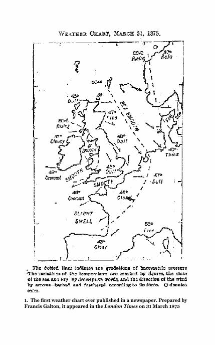
1. The first weather chart ever published in a newspaper. Prepared byFrancis Galton, it appeared in the London Times on 31 March 1875

If uncertainty due to errors of observation provides the seed that

chaos nurtures, then understanding such uncertainty can help us

better cope with chaos. Like Laplace, Galton was interested in the

‘theory of errors’ in the widest sense. To illustrate the ubiquitous

‘bell-shaped curve’ which so often seems to reflect measurement

errors, Galton created the ‘quincunx’, which is now called a Galton

Board; the most common version is shown on the left side of Figure

2. By pouring lead shot into the quincunx, Galton simulated a

random system in which each piece of shot has a 50:50 chance of

going to either side of every ‘nail’ that it meets, giving rise to a bell-

shaped distribution of lead. Note there is more here than the one-

off flap of a butterfly wing: the paths of two nearby pieces of lead

may stay together or diverge at each level. We shall return to Galton

Boards in Chapter 9, but we will use random numbers from the

bell-shaped curve as a model for noise many times before then. The

bell-shape can be seen at the bottom of the Galton Board on the left

of Figure 2, and we will find a smoother version towards the top of

Figure 10.

The study of chaos yields new insight into why weather forecasts

remain unreliable after almost two centuries. Is it due to our

missing minor details in today’s weather which then have major

impacts on tomorrow’s weather? Or is it because our methods,

while better than Fitzroy’s, remain imperfect? Poe’s early

atmospheric incarnation of the butterfly effect is complete with the

idea that science could, if perfect, predict everything physical. Yet

the fact that sensitive dependence would make detailed forecasts of

the weather difficult, and perhaps even limit the scope of physics,

has been recognized within both science and fiction for some time.

In 1874, the physicist James Clerk Maxwell noted that a sense of

proportion tended to accompany success in a science:

This is only true when small variations in the initial circumstances

produce only small variations in the final state of the system. In a

great many physical phenomena this condition is satisfied; but there

are other cases in which a small initial variation may produce a very

8

Ch

ao

s

great change in the final state of the system, as when the

displacement of the ‘points’ causes a railway train to run into

another instead of keeping its proper course.

This example is again atypical of chaos in that it is ‘one-off’

sensitivity, but it does serve to distinguish sensitivity and

uncertainty: this sensitivity is no threat as long as there is no

uncertainty in the position of the points, or in which train is on

which track. Consider pouring a glass of water near a ridge in the

2. Galton’s 1889 schematic drawings of what are now called ‘GaltonBoards’

9

Th

e e

me

rge

nce

of ch

ao

s

Rocky Mountains. On one side of this continental divide the water

finds its way into the Colorado River and to the Pacific Ocean, on

the other side the Mississippi River and eventually the Atlantic

Ocean. Moving the glass one way or the other illustrates

sensitivity: a small change in the position of the glass means a

particular molecule of water ends up in a different ocean. Our

uncertainty in the position of the glass might restrict our ability to

predict which ocean that molecule of water will end up in, but only

if that uncertainty crosses the line of the continental divide. Of

course, if we were really trying to do this, we would have to

question whether any such mathematical line actually divided

continents, as well as the other adventures the molecule of water

might have which could prevent it reaching the ocean. Usually,

chaos involves much more than a single one-off ‘tripping point’; it

tends to more closely resemble a water molecule that repeatedly

evaporates and falls in a region where there are continental divides

all over the place.

Nonlinearity is defined by what it is not (it is not linear). This kind

of definition invites confusion: how would one go about defining a

biology of non-elephants? The basic idea to hold in mind now is

that a nonlinear system will show a disproportionate response: the

impact of adding a second straw to a camel’s back could be much

bigger (or much smaller) than the impact of the first straw. Linear

systems always respond proportionately. Nonlinear systems need

not, giving nonlinearity a critical role in the origin of sensitive

dependence.

The Burns’ Day storm

But Mousie, thou art no thy lane,

In proving foresight may be vain:

The best-laid schemes o mice an men

Gang aft agley,

An lea’e us nought but grief an pain,

For promis’d joy!

10

Ch

ao

s

Still thou art blest, compar’d wi me!

The present only toucheth thee:

But och! I backward cast my e’e,

On prospects drear!

An forward, tho I canna see,

I guess an fear!

Robert Burns, ‘To A Mouse’ (1785)

Burns’ poem praises the mouse for its ability to live only in the

present, not knowing the pain of unfulfilled expectations nor the

dread of uncertainty in what is yet to pass. And Burns was writing

in the 18th century, when mice and men laid their plans with little

assistance from computing machines. While foresight may be pain,

meteorologists struggle to foresee tomorrow’s likely weather every

day. Sometimes it works. In 1990, on the anniversary of Burns’

birth, a major storm ripped through northern Europe, including the

British Isles, causing significant property damage and loss of life.

The centre of the storm passed over Burns’ home town in Scotland,

and it became known as the Burns’ Day storm. A weather chart

reflecting the storm at noon on 25 January is shown in the top

panel of Figure 4 (page 14). Ninety-seven people died in northern

Europe, about half of this number in Britain, making it the highest

death toll of any storm in 40 years; about 3 million trees were blown

down, and total insurance costs reached £2 billion. Yet the Burns’

Day storm has not joined the rogues’ gallery of famously failed

forecasts: it was well forecast by the Met Office.

In contrast, the Great Storm of 1987 is famous for a BBC television

meteorologist’s broadcast the night before, telling people not to

worry about rumours from France that a hurricane was about to

strike England. Both storms, in fact, managed gusts of over

100 miles per hour, and the Burns’ Day storm caused much

greater loss of life; yet 20 years after the event, the Great Storm of

1987 is much more often discussed, perhaps exactly because the

Burns’ Day storm was well forecast. The story leading up to this

forecast beautifully illustrates a different way that chaos in our

11

Th

e e

me

rge

nce

of ch

ao

s

models can impact our lives without invoking alternate worlds,

some with and some without butterflies.

In the early morning of 24 January 1990, two ships in the

mid-Atlantic sent routine meteorological observations from

positions that happened to straddle the centre of what would

become the Burns’ Day storm. The forecast models run with these

observations give a fine forecast of the storm. Running the model

again after the event showed that when these observations are

omitted, the model predicts a weaker storm in the wrong place.

Because the Burns’ Day storm struck during the day, the failure to

provide forewarning would have had a huge impact on loss of life,

so here we have an example where a few observations, had they

not been made, would have changed the forecast and hence the

course of human events. Of course, an ocean weather ship is

harder to misplace than a horse shoe nail. There is more to this

story, and to see its relevance we need to look into how weather

models ‘work’.

Operational weather forecasting is a remarkable phenomenon in

and of itself. Every day, observations are taken in the most remote

locations possible, and then communicated and shared among

national meteorological offices around the globe. Many different

nations use this data to run their computer models. Sometimes an

observation is subject to plain old mistakes, like putting the

temperature in the box for wind speed, or a typo, or a glitch in

transition. To keep these mistakes from corrupting the forecast,

incoming observations are subject to quality control: observations

that disagree with what the model is expecting (given its last

forecast) can be rejected, especially if there are no independent,

nearby observations to lend support to them. It is a well-laid plan.

Of course, there are rarely any ‘nearby’ observations of any sort in

the middle of the Atlantic, and the ship observations showed the

development of a storm that the model had not predicted would be

there, so the computer’s automatic quality control program simply

rejected these observations.

12

Ch

ao

s

3. Headline from The Times the day after the Burns’ Day storm

4. A modern weather chart reflecting the Burns’ Day storm as seenthrough a weather model (top) and a two-day-ahead forecast targetingthe same time showing a fairly pleasant day (bottom)

Luckily, the computer was overruled. An intervention forecaster

was on duty and realized that these observations were of great

value. His job was to intervene when the computer did something

obviously silly, as computers are prone to do. In this case, he tricked

the computer into accepting the observations. Whether or not to

take this action is a judgement call: there was no way to know at the

time which action would yield a better forecast. The computer was

‘tricked’, the observation was used. The storm was forecast, and

lives were saved.

There are two take-home messages here: the first is that when our

models are chaotic then small changes in our observations can have

large impacts on the quality of our foresight. An accountant looking

to reduce costs and computing the typical benefit of one particular

observation from any particular weather station is likely to vastly

underestimate the value of a future report from one of those

weather stations that falls at the right place at the right time, and

similarly the value of the intervention forecaster, who often has to

do nothing, literally. The second is that the Burns’ Day forecast

illustrates something a bit different from the butterfly effect.

Mathematical models allow us to worry about what the real future

will bring not by considering possible worlds, of which there may be

only one, but by contrasting different simulations of our model, of

which there can be as many as we can afford. As Burns might

appreciate, science gives us new ways to guess and new things to

fear. The butterfly effect contrasts different worlds: one world with

the nail and another world without that nail. The Burns effect

places the focus firmly on us and our attempts to make rational

decisions in the real world given only collections of different

simulations under various imperfect models. The failure to

distinguish between reality and our models, between observations

and mathematics, arguably between an empirical fact and scientific

fiction, is the root of much confusion regarding chaos both by the

public and among scientists. It was research into nonlinearity and

chaos that clarified yet again how import this distinction remains.

In Chapter 10, we will return to take a deeper look at how today’s

15

Th

e e

me

rge

nce

of ch

ao

s

weather forecasters would have used insights from their

understanding of chaos when making a forecast for this event.

We have now touched on the three properties found in chaotic

mathematical systems: chaotic systems are nonlinear, they are

deterministic, and they are unstable in that they display sensitivity

to initial condition. In the chapters that follow we will constrain

them further, but our real interests lie not only in the mathematics

of chaos, but also in what it can tell us about the real world.

Chaos and the real world: predictability and a21st-century demon

There is no more greater an error in science, than to believe that just

because some mathematical calculation has been completed, some

aspect of Nature is certain.

Alfred North Whitehead (1953)

What implications does chaos hold for our everyday lives? Chaos

impacts the ways and means of weather forecasting, which affect us

directly through the weather, and indirectly through economic

consequences both of the weather and of the forecasts themselves.

Chaos also plays a role in questions of climate change and our

ability to foresee the strength and impacts of global warming. While

there are many other things that we forecast, weather and climate

can be used to represent short-range forecasting and long-range

modelling, respectively. ‘When is the next solar eclipse?’ would be a

weather-like question in astronomy, while ‘Is the solar system

stable?’ would be a climate-like question. In finance, when to buy

100 shares of a given stock is a weather-like question, while a

climate-like question might address whether to invest in the stock

market or real estate.

Chaos has also had a major impact on the sciences, forcing a close

re-examination of what scientists mean by the words ‘error’ and

‘uncertainty’ and how these meanings change when applied to our

16

Ch

ao

s

world and our models. As Whitehead noted, it is dangerous to

interpret our mathematical models as if they somehow governed

the real world. Arguably, the most interesting impacts of chaos

are not really new, but the mathematical developments of the last

50 years have cast many old questions into a new light. For

instance, what impact would uncertainty have on a 21st-century

incarnation of Laplace’s demon which could not escape

observational noise?

Consider an intelligence that knew all the laws of nature precisely

and had good, but imperfect, observations of an isolated chaotic

system over an arbitrarily long time. Such an agent – even if

sufficiently vast to subject all this data to computationally exact

analysis – could not determine the current state of the system and

thus the present, as well as the future, would remain uncertain in

her eyes. While our agent could not predict the future exactly, the

future would hold no real surprises for her, as she could see what

could and what could not happen, and would know the probability

of any future event: the predictability of the world she could see.

Uncertainty of the present will translate into well-quantified

uncertainty in the future, if her model is perfect.

In his 1927 Gifford Lectures, Sir Arthur Eddington went to the

heart of the problem of chaos: some things are trivial to predict,

especially if they have to do with mathematics itself, while other

things seem predictable, sometimes:

A total eclipse of the sun, visible in Cornwall is prophesied for

11 August 1999 . . . I might venture to predict that 2 + 2 will be

equal to 4 even in 1999 . . . The prediction of the weather this time

next year . . . is not likely to ever become practicable . . . We should

require extremely detailed knowledge of present conditions, since

a small local deviation can exert an ever-expanding influence.

We must examine the state of the sun . . . be forewarned of volcanic

eruptions, . . . , a coal strike . . . , a lighted match idly thrown

away . . .

17

Th

e e

me

rge

nce

of ch

ao

s

Our best models of the solar system are chaotic, and our best

models of the weather appear to be chaotic: yet why was Eddington

confident in 1928 that the 1999 solar eclipse would occur? And

equally confident that no weather forecast a year in advance would

ever be accurate? In Chapter 10 we will see how modern weather

forecasting techniques designed to better cope with chaos helped

me to see that solar eclipse.

When paradigms collide: chaos and controversy

One of the things that has made working in chaos interesting over

the last 20 years has been the friction generated when different

ways of looking at the world converge on the same set of

observations. Chaos has given rise to a certain amount of

controversy. The studies that gave birth to chaos have

revolutionized not only the way professional weather forecasters

forecast but even what a forecast consists of. These new ideas often

run counter to traditional statistical modelling methods, and still

produce both heat and light on how best to model the real world.

This battle is broken into skirmishes by the nature of the field and

our level of understanding in the particular system of which a

question is asked, be it the population of voles in Scandinavia,

a mathematical calculation to quantify chaos, the number of

spots on the Sun’s surface, the price of oil delivered next month,

tomorrow’s maximum temperature, or the date of the last ever solar

eclipse.

The skirmishes are interesting, but chaos offers deeper insights

even when both sides are fighting for traditional advantage, say, the

‘best’ model. Here studies of chaos have redefined the high ground:

today we are forced to reconsider new definitions for what

constitutes the best model, or even a ‘good’ model. Arguably, we

must give up the idea of approaching Truth, or at least define a

wholly new way of measuring our distance from it. The study of

chaos motivates us to establish utility without any hope of achieving

perfection, and to give up many obvious home truths of forecasting,

18

Ch

ao

s

like the naıve idea that a good forecast consists of a prediction that

is close to the target. This did not appear naıve before we

understood the implications of chaos.

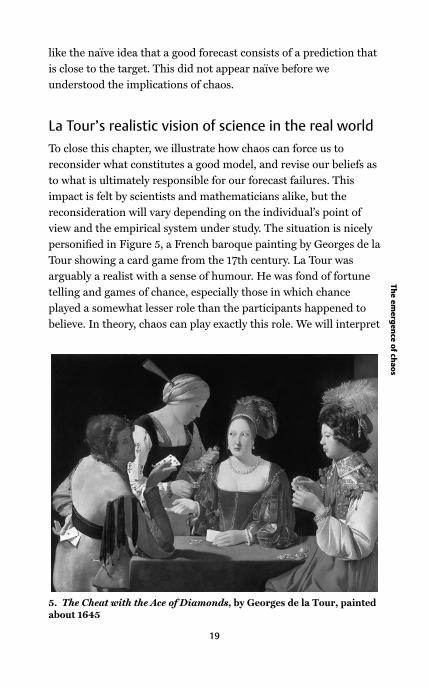
La Tour’s realistic vision of science in the real world

To close this chapter, we illustrate how chaos can force us to

reconsider what constitutes a good model, and revise our beliefs as

to what is ultimately responsible for our forecast failures. This

impact is felt by scientists and mathematicians alike, but the

reconsideration will vary depending on the individual’s point of

view and the empirical system under study. The situation is nicely

personified in Figure 5, a French baroque painting by Georges de la

Tour showing a card game from the 17th century. La Tour was

arguably a realist with a sense of humour. He was fond of fortune

telling and games of chance, especially those in which chance

played a somewhat lesser role than the participants happened to

believe. In theory, chaos can play exactly this role. We will interpret

5. The Cheat with the Ace of Diamonds, by Georges de la Tour, paintedabout 1645

19

Th

e e

me

rge

nce

of ch

ao

s

this painting to show a mathematician, a physicist, a statistician,

and a philosopher engaged in an exercise of skill, dexterity, insight,

and computational prowess; this is arguably a description for doing

science, but the task at hand here is a game of poker. Exactly who is

who in the painting will remain open, as we will return to these

personifications of natural science throughout the book. The

insights chaos yields vary with the perspective of the viewer, but a

few observations are in order.

The impeccably groomed young man on the right is engaged in

careful calculations, no doubt a probability forecast of some nature;

he is currently in possession of a handsome collection of gold coins

on the table. The dealer plays a critical role, without her there is no

game to be played; she provides the very language within which we

communicate, yet she seems to be in nonverbal communication

with the handmaiden. The role of the handmaiden is less clear; she

is perhaps tangential, but then again the provision of wine will

influence the game, and she herself may feature as a distraction.

The roguish character in ramshackle dress with bows untied is

clearly concerned with the real world, not mere appearances in

some model of it; his left hand is extracting one of several aces of

diamonds from his belt, which he is about to introduce into the

game. What then do the ‘probabilities’ calculated by the young man

count for, if, in fact, he is not playing the game his mathematical

model describes? And how deep is the insight of our rogue? His

glance is directed to us, suggesting that he knows we can see his

actions, perhaps even that he realizes that he is in a painting?

The story of chaos is important because it enables us to see the

world from the perspective of each of these players. Are we merely

developing the mathematical language with which the game is

played? Are we risking economic ruin by over-interpreting some

potentially useful model while losing sight of the fact that it, like all

models, is imperfect? Are we only observing the big picture, not

entering the game directly but sometimes providing an interesting

distraction? Or are we manipulating those things we can change,

20

Ch

ao

s

acknowledging the risks of model inadequacy, and perhaps even our

own limitations, due to being within the system? To answer these

questions we must first examine several of the many jargons of

science in order to be able to see how chaos emerged from the noise

of traditional linear statistics to vie for roles both in understanding

and in predicting complicated real-world systems. Before the

nonlinear dynamics of chaos were widely recognized within science,

these questions fell primarily in the domain of the philosophers;

today they reach out via our mathematical models to physical

scientists and working forecasters, changing the statistics of

decision support and even impacting politicians and policy makers.

21

Th

e e

me

rge

nce

of ch

ao

s

Chapter 2

Exponential growth,

nonlinearity, common sense

One of the most pervasive myths about chaotic systems is that they

are impossible to predict. To expose the fallacy of this myth, we

must understand how uncertainty in a forecast grows as we predict

further and further into the future. In this chapter we investigate

the origin and meaning of exponential growth, since on average a

small uncertainty will grow exponentially fast in a chaotic system.

There is a sense in which this phenomenon really does imply a

‘faster’ growth of uncertainty than that found in our traditional

ideas of how error and uncertainty grow as we forecast further into

the future. Nevertheless, chaos can be easy to predict, sometimes.

Chess, rice, and Leonardo’s rabbits:exponential growth

An oft-told story about the origin of the game of chess illustrates

nicely the speed of exponential growth. The story goes that a king of

ancient Persia was so pleased when first presented with the game

that he wanted to reward the game’s creator, Sissa Ben Dahir. A

chess board has 64 squares arranged in an 8 by 8 pattern; for his

reward, Ben Dahir requested what seemed a quite modest sum

of rice determined using the new chess board: one grain of rice

was to be put on the first square of the board, two to be put on

the second, four for the third, eight for the fourth, and so on,

doubling the number on each square until the 64th was reached. A

22

mathematician will often call any rule for generating one number

from another one a mathematical map, so we’ll refer to this simple

rule (‘double the current value to generate the next value’) as the

Rice Map.

Before working out just how much rice Ben Dahir has asked for, let

us consider the case of linear growth where we have one grain on

the first square, two on the second square, three on the third, and so

on until we need 64 for the last square. In this case we have a total

of 64 + 63 + 62 + . . . + 3 + 2 + 1, or around 1,000 grains. Just for

comparison, a 1 kilogram bag of rice contains a few tens of

thousands of grains.

The Rice Map requires one grain for the first square, then two for

the second, four for the third, then 8, 16, 32, 64, and 128 for the last

square of the first row. On the third square of the second row, we

pass 1,000 and before the end of the second row there is a square

which exhausts our bag of rice. To fill the next square alone will

require another entire bag, the following square two bags, and so

on. Some square in the third row will require a volume of rice

comparable to a small house, and we will have enough rice to fill the

Royal Albert Hall well before the end of the fifth row. Finally, the

64th square alone will require billions and billions, or to be exact,

263 (= 9, 223, 372, 036, 854, 775, 808) grains, for a total of

18,446,744,073,709,551,615 grains. That is a non-trivial quantity of

rice! It is something like the entire world’s rice production over two

millennia. Exponential growth quickly grows out of all proportion.

By comparing the amount of rice on a given square in the case of

linear growth with the amount of rice on the same square in the

case of exponential growth, we quickly see that exponential is much

faster than linear growth: on the fourth square we already have

twice as many grains in the exponential case as in the linear case

(8 in the first, only 4 in the second), and by the eighth square, at the

end of the first row, the exponential case has 16 times more!

Soon thereafter we have the astronomical numbers.

23

Ex

po

ne

ntia

l gro

wth

, no

nlin

ea

rity, co

mm

on

sen

se

Of course, we hid the values of some parameters in the example

above: we could have made the linear growth faster by adding

not one additional grain for each square, but instead, say,

1,000 additional grains. This parameter, the number of

additional grains, defines the constant of proportionality between

the number of the square and the number of grains on that

square, and gives us the slope of the linear relationship between

them. There is also a parameter in the exponential case: on

each step we increased the number of grains by a factor of two,

but it could have been a factor of three, or a factor of one and a

half.

One of the surprising things about exponential growth is that

whatever the values of these parameters, there will come a time at

which exponential growth surpasses any linear growth, and will

soon thereafter dwarf linear growth, no matter how fast the linear

growth is. Our ultimate interest is not in rice on a chess board, but

in the dynamics of uncertainty in time. Not just the growth of a

population, but the growth of our uncertainty in a forecast of the

future size of that population. In the forecasting context, there will

come a time at which an exponentially growing uncertainty which is

very small today will surpass a linearly growing uncertainty which is

today much larger. And the same thing happens when contrasting

exponential growth with growth proportional to the square of time,

or to the cube of time, or to time raised to any power (in symbols:

steady exponential growth will eventually surpass the growth

proportional to t2 or t3 or tn for any value of n.). It is for this reason

among others that exponential growth is mathematically

distinguished, and taken to provide a benchmark for defining

chaos. It has also contributed to the widespread but fundamentally

mistaken impression that chaotic systems are hopelessly

unpredictable. Ben Dahir’s chess board illustrates that there is a

deep sense in which exponential growth is faster than linear growth.

To place this in the context of forecasting, we move forward a few

hundred years in time and a few hundred miles northwest, from

Persia to Italy.

24

Ch

ao

s

At the beginning of the 13th century, Leonardo of Pisa posed a

question of population dynamics: given a newborn pair of rabbits in

a large, lush, walled garden, how many pairs of rabbits will we have

in one year if their nature is for each mature pair to breed and

produce a new pair every month, and newborn rabbits mature in

their second month? In the first month we have one juvenile pair. In

the second month this pair matures and breeds to produce a new

pair in the third month. So in the third month, we have one mature

pair and one newborn pair. In the fourth month we once again have

one new born pair from the original pair of rabbits and now two

mature pairs for a total of three pairs. In the fifth month, two new

pairs are born (one from each mature pair), and we have three

mature pairs for a total of five pairs. And so on.

So what does this ‘population dynamic’ look like? In the first month

we have one immature pair, in the second month we have one

mature pair, in the third month we have one mature pair and a new

immature pair, in the fourth month we have two mature pairs and

one immature pair, in the fifth month we have three mature pairs

and two immature.

If we count up all the pairs each month, the numbers are 1, 1, 2, 3, 5,

8, 13, 21 . . . . Leonardo noted that the next number in the series is

always the sum of the previous two numbers (1 + 1 = 2, 2 + 1 = 3,

3 + 2 = 5, . . . ) which makes sense, as the previous number is the

number we had last month (in our model all rabbits survive no

matter how many there are), and the penultimate number is the

number of mature pairs (and thus the number of new pairs arriving

this month).

Now it gets a bit tedious to write ‘and in the sixth month we have

12 pairs of rabbits’, so scientists often use a short-hand X for the

number of pairs of rabbits and X6 to denote the number of pairs in

month six. And since the series 1, 1, 2, 3, 5, 8, . . . reflects how the

population of rabbits evolves in time, this series and others like it

are called time series. The Rabbit Map is defined by the rule:

25

Ex

po

ne

ntia

l gro

wth

, no

nlin

ea

rity, co

mm

on

sen

se

Add the previous value of X to the current value of X, and take

the sum as the new value of X.

The numbers in the series 1, 1, 2, 3, 5, 8, 13, 21, 34 . . . are

called Fibonacci numbers (Fibonacci was a nickname of

Leonardo of Pisa), and they arise again and again in nature: in the

structure of sunflowers, pine cones, and pineapples. They are of

interest here because they illustrate exponential growth in time,

almost. The crosses in Figure 6 are Fibonacci’s points – the

rabbit population as a function of time – while the solid line

reflects two raised to the power λt, or in symbols 2λt , where t is

the time in months and λ is our first exponent. Exponents which

multiply time in the superscript are a useful way of quantifying

uniform exponential growth. In this case, λ is equal to the

logarithm of a number called the golden mean, a very special

number which is discussed in the Very Short Introduction to

Mathematics.

6. The series of crosses showing the number of pairs of rabbits eachmonth (Fibonacci numbers); the smooth curve they lie near is therelated exponential growth

26

Ch

ao

s

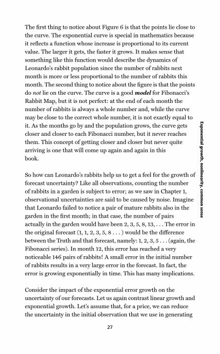
The first thing to notice about Figure 6 is that the points lie close to

the curve. The exponential curve is special in mathematics because

it reflects a function whose increase is proportional to its current

value. The larger it gets, the faster it grows. It makes sense that

something like this function would describe the dynamics of

Leonardo’s rabbit population since the number of rabbits next

month is more or less proportional to the number of rabbits this

month. The second thing to notice about the figure is that the points

do not lie on the curve. The curve is a good model for Fibonacci’s

Rabbit Map, but it is not perfect: at the end of each month the

number of rabbits is always a whole number and, while the curve

may be close to the correct whole number, it is not exactly equal to

it. As the months go by and the population grows, the curve gets

closer and closer to each Fibonacci number, but it never reaches

them. This concept of getting closer and closer but never quite

arriving is one that will come up again and again in this

book.

So how can Leonardo’s rabbits help us to get a feel for the growth of

forecast uncertainty? Like all observations, counting the number

of rabbits in a garden is subject to error; as we saw in Chapter 1,

observational uncertainties are said to be caused by noise. Imagine

that Leonardo failed to notice a pair of mature rabbits also in the

garden in the first month; in that case, the number of pairs

actually in the garden would have been 2, 3, 5, 8, 13, . . . The error in

the original forecast (1, 1, 2, 3, 5, 8 . . . ) would be the difference

between the Truth and that forecast, namely: 1, 2, 3, 5 . . . (again, the

Fibonacci series). In month 12, this error has reached a very

noticeable 146 pairs of rabbits! A small error in the initial number

of rabbits results in a very large error in the forecast. In fact, the

error is growing exponentially in time. This has many implications.

Consider the impact of the exponential error growth on the

uncertainty of our forecasts. Let us again contrast linear growth and

exponential growth. Let’s assume that, for a price, we can reduce

the uncertainty in the initial observation that we use in generating

27

Ex

po

ne

ntia

l gro

wth

, no

nlin

ea

rity, co

mm

on

sen

se

our forecast. If the error growth is linear, and we reduce our

initial uncertainty by a factor of ten, then we can forecast the

system ten times longer before our uncertainty exceeds the same

threshold. If we reduce the initial uncertainty by a factor of 1,000,

then we can get forecasts of the same quality 1,000 times longer.

This is an advantage of linear models. Or, more accurately, this is

an apparent advantage of studying only linear systems. By

contrast, if the model is nonlinear and the uncertainty grows

exponentially, then we may reduce our initial uncertainty by a

factor of ten yet only be able to forecast twice as long with the

same accuracy. In that case, assuming the exponential growth in

uncertainty is uniform in time, reducing the uncertainty by a

factor of 1,000 will only increase our forecast range at the same

accuracy by a factor of eight. Now reducing the uncertainty in a

measurement is rarely free (we have to hire someone else to count

the rabbits a second time), and large reductions of uncertainty

can be expensive, so when uncertainty grows exponentially fast,

the cost sky-rockets. Attempting to achieve our forecast goals by

reducing uncertainty in initial conditions can be tremendously

expensive.

Luckily, there is an alternative that allows us to accept the simple

fact that we can never be certain that any observation has not been

corrupted by noise. In the case of rabbits or grains of rice, it seems

there really is a fact of the matter, a whole number that reflects the

correct answer. If we reduce the uncertainty in this initial condition

to zero then we can predict without error. But can we ever really be

certain of the initial condition? Might there not be another bunny

hiding in the noise? While our best guess is that there is one pair in

the garden, there might be two, or three, or more (or perhaps zero).

When we are uncertain of the initial condition, we can examine the

diversity of forecasts under our model by making an ensemble of

forecasts: one forecast started from each initial condition we think

plausible. So one member of the ensemble will start with X equal to

one, another ensemble member will start with X equals two, and so

on. How should we divide our limited resources between computing

28

Ch

ao

s

more ensemble members and making better observations of the

current number of rabbits in the garden?

In the Rabbit Map, differences between the forecasts of different

members of the ensemble will grow exponentially fast, but with an

ensemble forecast we can see just how different they are and use

this as a measure of our uncertainty in the number of rabbits we

expect at any given time. In addition, if we carefully count the

number of rabbits after a few months, we can all but rule out some

of the individual ensemble members. Each of these ensemble

members was started from some estimate of the number of rabbits

that were in the garden originally, so ruling an ensemble member

out in effect gives us more information about the original number of

rabbits. Of course, this information need only prove accurate if our

model is literally perfect, meaning, in this case, that our Rabbit Map

captures the reproductive behaviour and longevity of our rabbits

exactly. But if our model is perfect, then we can use future

observations to learn about the past; this process is called noise

reduction. If it turns out that our model is not perfect, then we may

end up with incoherent results.

But what if we were measuring something that is not a whole

number, like temperature, or the position of a planet? And is

temperature in an imperfect weather model exactly the same thing

as temperature in the real world? It was these questions that

initially interested our philosopher in chaos. First, we should

consider the more pressing question of why rabbits have not taken

over the world in the 9,000 months since 1202?

Stretching, folding, and the growth of uncertainty

The study of chaos lends credence to the meteorological maxim that

no forecast is complete without a useful estimate of forecast

uncertainty: if we know our initial condition is uncertain then we

are not only interested in the prediction per se, but equally in

learning what the likely forecast error will be. Forecast error for any

29

Ex

po

ne

ntia

l gro

wth

, no

nlin

ea

rity, co

mm

on

sen

se

Exponential growth: an example fromMiss Nagel’s third grade class

A few months ago, I received an email written by an old

friend of mine from elementary school. It contained another

email that had originated from a third grader in North

Carolina whose class was studying geography. It requested

that everyone who read the email send a reply to the school

stating where they lived, and the class would locate that place

on a school globe. It also requested that each reader pass on

the email to ten friends.

I did not forward the message to anyone, but I did write an

email to Miss Nagel’s class stating that I was in Oxford,

England. I also suggested that they tell their mathematics

teacher about their experiment and use it as an example to

illustrate exponential growth: if they sent the message to ten

people, and the next day each of them sent it to ten more

people, that would be 100 on day three, 1,000 on day four,

and more emails than there are email addresses within a

week or so. In a real system, exponential growth cannot go

on forever: eventually we run out of rice, or garden space, or

new email addresses. It is often the resources that limit

growth: even a lush garden provides only a finite amount

of rabbit food. There are limits to growth which bound

populations, if not our models of populations.

I never found out whether Miss Nagel’s class learned their

lesson in exponential growth. The only answer I ever

received was an automated reply stating that the school’s

email in-box had exceeded its quota and had been closed.

30

Ch

ao

s

real system should not grow without limit; even if we start with a

small error like one grain or one rabbit, the forecast error will not

grow arbitrarily large (unless we have a very naıve forecaster), but

will saturate near some limiting value, as would the population

itself. Our mathematician has a way to avoid ludicrously large

forecast errors (other than naıveté), namely by making the initial

uncertainty infinitesimally small – smaller than any number you

can think of, yet greater than zero. Such an uncertainty will stay

infinitesimally small for all time, even if it grows exponentially fast.

Physical factors, like the total amount of rabbit food in the garden

or the amount of disk space on an email system, limit growth in

practice. The limits are intuitive even if we do not know exactly

what causes them: I think I have lost my keys in the car park; of

course they might be several miles from there, but it is exceedingly

unlikely that they are farther away than the moon. I do not need to

understand or believe the laws of gravity to appreciate this.

Similarly, weather forecasters are rarely more than 100 degrees off,

even for a forecast one year in advance! Even inadequate models

can usually be constrained so that their forecast errors are bounded.

Whenever our model goes into never-never land (suggesting values

where no data have ever gone before), then something is likely to

give, unless something in our model has already broken. Often, as

our uncertainty grows too large, it starts to fold back on itself.

Imagine kneading dough, or a toffee machine continuously

stretching and folding toffee. An imaginary line of toffee connecting

two very nearby grains of sugar will grow longer and longer as these

two grains separate under the action of the machine, but before it

becomes bigger than the machine itself, this line will be folded back

into itself, forming a horrible tangle. The distance between the

grains of sugar will stop growing, even as the string of toffee

connecting them continues to grow longer and longer, becoming a

more and more complicated tangle. The toffee machine gives us a

way to envision limits to the growth of prediction error whenever

our model is perfect. In this case, the error is the growing distance

31

Ex

po

ne

ntia

l gro

wth

, no

nlin

ea

rity, co

mm

on

sen

se

between the True state and our best guess of that state: any

exponential growth of error would correspond only to the rapid

initial growth of the string of toffee. But if our forecasts are not

going to zoom away towards infinity (the toffee must stay in the

machine, only a finite number of rabbits will fit in the garden, and

the like), then eventually the line connecting Truth and our forecast

will be folded over on itself. There is simply nowhere else for it to

grow into. In many ways, identifying the movement of a grain of

sugar in the toffee machine with the evolution of the state of a

chaotic system in three dimensions is a useful way to visualize

chaotic motion.

We want to require a sense of containment for chaos, since it is

hardly surprising that it is difficult to predict things that are flying

apart to infinity, but we do not want to impose so strict a condition

as requiring a forecast to never exceed some limited value, no

matter how big that value might be. As a compromise, we require

the system to come back to the vicinity of its current state at some

point in the future, and to do so again and again. It can take as long

as it wants to come back, and we can define coming back to mean

returning closer to the current point than we have ever seen it

return before. If this happens, then the trajectory is said to be

recurrent. The toffee again provides an analogy: if the motion was

chaotic and we wait long enough, our two grains of sugar will again

come back close together, and each will pass close to where it was at

the beginning of the experiment, assuming no one turns off the

machine in the meantime.

32

Ch

ao

s

Chapter 3

Chaos in context:

determinism, randomness,

and noise

All linear systems resemble one another, each nonlinear system is

nonlinear in its own way.

After Tolstoy’s Anna Karenina

Dynamical systems

Chaos is a property of dynamical systems. And a dynamical system

is nothing more than a source of changing observations: Fibonacci’s

imaginary garden with its rabbits, the Earth’s atmosphere as

reflected by a thermometer at London’s Heathrow airport, the

economy as observed through the price of IBM stock, a computer

program simulating the orbit of the moon and printing out the

date and location of each future solar eclipse.

There are at least three different kinds of dynamical systems. Chaos

is most easily defined in mathematical dynamical systems. These

systems consist of a rule: you put a number in and you get a new

number out, which you put back in, to get yet a newer number out,

which you put back in. And so on. This process is called iteration.

The number of rabbits each month in Fibonacci’s imaginary garden

is a perfect example of a time series from this kind of system. A

second type of dynamical system is found in the empirical world of

the physicist, the biologist, or the stock market trader. Here, our

sequence of observations consists of noisy measurements of reality,

33

which are fundamentally different from the noise-free numbers of

the Rabbit Map. In these physical dynamical systems – the Earth’s

atmosphere and Scandinavia’s vole population, for example –

numbers represent the state, whereas in the Rabbit Map they were

the state. To avoid needless confusion, it is useful to distinguish a

third case when a digital computer performs the arithmetic

specified by a mathematical dynamical system; we will call this a

computer simulation – computer programs that produce TV

weather forecasts are a common example. It is important to

remember that these are different kinds of systems and that each is

a different beast: our best equations for the weather differ from our

best computer models based on those equations, and both of these

systems differ from the real thing the Earth’s atmosphere itself.

Confusingly, the numbers from each of our three types of systems

are called time series, and we must constantly struggle to keep in

mind the distinction between what these are time series of: a

number of imaginary rabbits, the True temperature at the airport (if

such a thing exists), a measurement representing that temperature,

and a computer simulation of that temperature.

The extent to which these differences are important depends on

what we aim to do. Like la Tour’s card players, scientists,

mathematicians, statisticians, and philosophers each have different

talents and aims. The physicist may aim to describe the

observations with a mathematical model, perhaps testing the

model by using it to predict future observations. Our physicist is

willing to sacrifice mathematical tractability for physical relevance.

Mathematicians like to prove things that are true for a wide range

of systems, but they value proof so highly that they often do not

care how widely they must restrict that range to have it; one

should almost always be wary whenever a mathematician is

heard to say ‘almost every’. Our physicist must be careful not to

forget this and confuse mathematical utility with physical

relevance; physical intuitions should not be biased by the properties

of ‘well-understood’ systems designed only for their mathematical

tractability.

34

Ch

ao

s

Our statistician is interested in describing interesting statistics

from the time series of real observations and in studying the

properties of dynamical systems that generate time series which

look like the observations, always taking care to make as few

assumptions as possible. Finally, our philosopher questions the

relationships among the underlying physical system that we claim

generated the observations, the observations themselves, and the

mathematical models or statistical techniques that we created to

analyse them. For example, she is interested in what we can know

about the relationship between the temperature we measure and

the true temperature (if such a thing exists), and in whether the

limits on our knowledge are merely practical difficulties we might

resolve or limits in principle that we can never overcome.

Mathematical dynamical systems and attractors

We commonly find four different types of behaviour in time series.

They can (i) grind to a halt and more or less repeat the same fixed

number over and over again, (ii) bounce around in a closed loop like

a broken record, periodically repeating the same pattern: exactly

the same series of numbers over and over, (iii) move in a loop that

has more than one period and so does not quite repeat exactly but

comes close, like the moment of high tide drifting through the time

of day, or (iv) forever jump about wildly, or perhaps even calmly,

displaying no obvious pattern. The fourth type looks random, yet

looks can be deceiving. Chaos can look random but it is not random.

In fact, as we have learned to see better, chaos often does not even

look all that random to us anymore. In the next few pages we will

introduce several more maps, though perhaps without the rice or

rabbits. We need these maps in order to generate interesting

artefacts for our tour in search of the various types of behaviour just

noted. Some of these maps were generated by mathematicians for

this very purpose, although our physicist might argue, with reason,

that a given map was derived by simplifying physical laws. In truth,

the maps are simple enough to have each come about in several

different ways.

35

Ch

ao

s in co

nte

xt: d

ete

rmin

ism, ra

nd

om

ne

ss, an

d n

oise

Before we can produce a time series by iterating a map, we need

some number to start with. This first number is called an initial

condition, an initial state that we define, discover, or arrange for

our system to be. As in Chapter 2, we adopt the symbol X as short-

hand for a state of our system. The collection of all possible states X

is called the state space. For Fibonacci’s imaginary rabbits, this

would be the set of all whole numbers. Suppose our time series is

from a model of the average number of insects per square mile at

mid-summer each year. In that case, X is just a number and the

state space, being the collection of all possible states, is then a line.

It sometimes takes more than one number to define the state, and if

so X will have more than one component. In predator-prey models,

for instance, the populations of both are required and X has two

components: it is a vector. When X is a vector containing both the

number of voles (prey) and the number of weasels (predators) on

the first of January each year, then the state space will be a two-

dimensional surface – a plane – that contains all pairs of numbers.

If X has three components (say, voles, weasels, and annual

snowfall), then the state space is a three-dimensional space

containing all triplets of numbers. Of course, there is no reason to

stop at three components; although the pictures become more

challenging to draw in higher dimensions, modern weather models

have over 10,000,000 components. For a mathematical system,

X can even be a continuous field, like the height of the surface

of the ocean or the temperature at every point on the surface of

the Earth. However, our observations of physical systems will

never be more complicated than a vector, and since we will only

measure a finite number of things, our observations will always be

finite-dimensional vectors. For the time being, we will consider the

case in which X is a simple number, such as one-half.

Recalling that a mathematical map is just a rule that transforms one

set of values into the next set of values, you can define the

Quadrupling Map by the rule:

Multiply X by four to form the new value of X.

36

Ch

ao

s

Given an initial condition, like X equals one-half, this mathematical

dynamical system produces a time series of values of X, in this case

½ × 4 = 2, 2 × 4 = 8, 8 × 4 = 32 . . . and the time series is 0.5, 2, 8, 32,

128, 512, 2048 . . . And so on. This series just gets bigger and

bigger and, dynamically speaking, that is not so interesting. If a

time series of X grows without limit like this one does, we call it

unbounded. In order to get a dynamical system where X is bounded,

we’ll take a second example, the Quartering Map:

Take X divided by four as the new X

Starting at X = ½ yields the time series 1/8, 1/32, 1/128, . . . . At first

sight, this is not very exciting since X rapidly shrinks towards zero.

But in fact, the Quartering Map has been carefully designed to

illustrate special mathematical properties. The origin – the state

X = 0 – is a fixed point: if we start there we will never leave, since

zero divided by four is again zero. The origin is also our first

attractor; under the Quartering Map the origin is the inevitable if

unreachable destination: if we start with some other value of X, we

never actually make it to the attractor, although we get close as the

number of iterations increases without limit. How close? Arbitrarily

close. As close as you like. Infinitesimally close, meaning closer

than any number you can name. Name a number, any number, and

we can work out how many iterations are required after which X

will remain closer to zero than that number. Getting arbitrarily

close to an attractor as time goes on while never quite reaching it is

a common feature of many time series from nonlinear systems. The

pendulum provides a physical analogue: each swing will be smaller

than the last, an effect we blame on air resistance and friction. The

analogue of the attractor in this case is the motionless pendulum

hanging straight down. We will have more to say about attractors

after we have added a few more dynamical systems to our

menagerie.

In the Full Logistic Map, time series from almost every X bounces

around irregularly between zero and one forever:

37

Ch

ao

s in co

nte

xt: d

ete

rmin

ism, ra

nd

om

ne

ss, an

d n

oise

Subtract X2 from X, multiply the difference by four and take the

result as the new X.

If we multiply components of state variables by other components,

things become nonlinear. What is the time series in this case if we

again start with X equals one-half? Starting with ½, X minus X2 is

¼, times four is one, so our new value is one. Continuing with X

now equal to one, we have X minus X2 is zero. But four times zero is

always zero, so we’ll get zeros forever. And our time series is 0.5, 1,

0, 0, 0 . . . This does not blow up, but it is hardly exciting; recall the

warning about ‘almost every’.

The order of the numbers in a time series is important, whether the

series reflects monthly values of Fibanocci’s rabbits or iterations of

the Full Logistic Map. Using the short-hand suggested in Chapter 2,

we will write X5 for the fifth new value of X, and X0 for the initial

state (or observation), and in general Xi for the ith value. Whether

we are iterating the map or taking observations, i is always an

integer and is often called ‘time’.

In the Full Logistic Map with X0 is equal to 0.5, X1 is equal to 1, X2

is 0, X3 is 0, X4 is 0, and Xi will be zero for all i greater than four as

well. So the origin is again a fixed point. But under the Full Logistic

Map small values of X grow (you can check this with a hand

calculator), X = 0 is unstable and so the origin is not an attractor.

A time series started near the origin is in fact unlikely to take one of

the first three options noted at the opening of this section, but to

bounce about chaotically forever.

Figure 7 shows a time series starting near X0 equals 0.876; it

represents a chaotic time series from the Full Logistic Map. But

look at it closely: does it really look completely unpredictable? It

looks like small values of X are followed by small values of X, and

that there is a tendency for the time series to linger whenever it is

near three-quarters. Our physicist would look at this series and

expect it to be predictable at least sometimes, while, after a few

38

Ch

ao

s

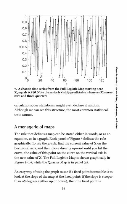
calculations, our statistician might even declare it random.

Although we can see this structure, the most common statistical

tests cannot.

A menagerie of maps

The rule that defines a map can be stated either in words, or as an

equation, or in a graph. Each panel of Figure 8 defines the rule

graphically. To use the graph, find the current value of X on the

horizontal axis, and then move directly upward until you hit the

curve; the value of this point on the curve on the vertical axis is

the new value of X. The Full Logistic Map is shown graphically in

Figure 8 (b), while the Quarter Map is in panel (a).

An easy way of using the graph to see if a fixed point is unstable is to

look at the slope of the map at the fixed point: if the slope is steeper

than 45 degrees (either up or down); then the fixed point is

7. A chaotic time series from the Full Logistic Map starting nearX0 equals 0.876. Note the series is visibly predictable whenever X is nearzero and three-quarters

39

Ch

ao

s in co

nte

xt: d

ete

rmin

ism, ra

nd

om

ne

ss, an

d n

oise

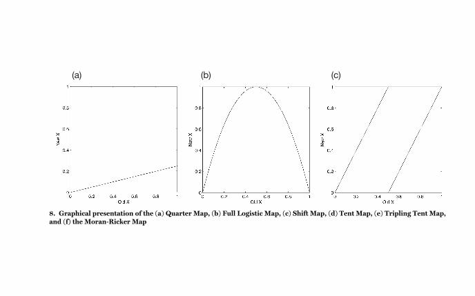
8. Graphical presentation of the (a) Quarter Map, (b) Full Logistic Map, (c) Shift Map, (d) Tent Map, (e) Tripling Tent Map,and (f) the Moran-Ricker Map

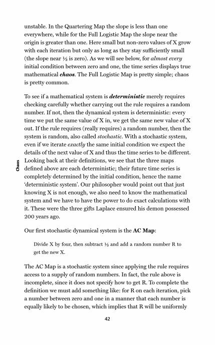
unstable. In the Quartering Map the slope is less than one

everywhere, while for the Full Logistic Map the slope near the

origin is greater than one. Here small but non-zero values of X grow

with each iteration but only as long as they stay sufficiently small

(the slope near ½ is zero). As we will see below, for almost every

initial condition between zero and one, the time series displays true

mathematical chaos. The Full Logistic Map is pretty simple; chaos

is pretty common.

To see if a mathematical system is deterministic merely requires

checking carefully whether carrying out the rule requires a random

number. If not, then the dynamical system is deterministic: every

time we put the same value of X in, we get the same new value of X

out. If the rule requires (really requires) a random number, then the

system is random, also called stochastic. With a stochastic system,

even if we iterate exactly the same initial condition we expect the

details of the next value of X and thus the time series to be different.

Looking back at their definitions, we see that the three maps

defined above are each deterministic; their future time series is

completely determined by the initial condition, hence the name

‘deterministic system’. Our philosopher would point out that just

knowing X is not enough, we also need to know the mathematical

system and we have to have the power to do exact calculations with

it. These were the three gifts Laplace ensured his demon possessed

200 years ago.

Our first stochastic dynamical system is the AC Map:

Divide X by four, then subtract ½ and add a random number R to

get the new X.

The AC Map is a stochastic system since applying the rule requires

access to a supply of random numbers. In fact, the rule above is

incomplete, since it does not specify how to get R. To complete the

definition we must add something like: for R on each iteration, pick

a number between zero and one in a manner that each number is

equally likely to be chosen, which implies that R will be uniformly

42

Ch

ao

s

distributed between zero and one and that the probability of the

next value of R falling in an interval of values is proportional to the

width of that interval.

What rule do we use to pick R? It could not be a deterministic rule,

since then R would not be random. Arguably, there is no finite rule

for generating values of R. This has nothing to do with needing

uniform numbers between zero and one. We’d have the same

problem if we wanted to generate random numbers which

mimicked Galton’s ‘bell-shape’ distribution. We will have to rely on

our statistician to somehow get us the random numbers we need;

hereafter we’ll just state whether they have a uniform distribution

or the bell-shaped distribution.

In the AC Map, each value of R is used within the map, but there is

another class of random maps – called Iterated Function Systems,

or IFS for short – which appear to use the value of R not in a

formula but to make a decision as to what to do. One example is the

Middle Thirds IFS Map, which will come in handy later when we

try to work out the properties of maps from the time series that they

generate. The Middle Thirds IFS Map is:

Take a random number R from a uniform distribution between zero

and one.

If R is less than a half, take X/3 as the new X

Otherwise take 1 – X/3 as the new X.

So now we have a few mathematical systems, and we can easily

tell if they are deterministic or stochastic. What about computer

simulations? Digital computer simulations are always

deterministic. And as we shall see in Chapter 7, the time series

from a digital computer is either on an endless loop of values

repeating itself periodically, over and over again, or it is on its

way towards such a loop. This first part of a time series in which

no value is repeated, the trajectory is evolving towards a periodic

loop but has not reached it, is called a transient. In

mathematical circles, this word is something of an insult, since

43

Ch

ao

s in co

nte

xt: d

ete

rmin

ism, ra

nd

om

ne

ss, an

d n

oise

mathematicians prefer to work with long-lived things, not mere

transients. While mathematicians avoid transients, physical

scientists may never see anything else and, as it turns out, digital

computers cannot maintain them. The digital computers that

have proven critical in advancing our understanding of chaos

cannot, ironically, display true mathematical chaos themselves.

Neither can a digital computer generate random numbers. The

so-called random number generators on digital computers and

hand calculators are, in fact, only pseudo-random number

generators; one of the earliest of these generators was even based

on the Full Logistic Map! The difference between mathematical

chaos and computer simulations, like that between random

numbers and pseudo-random numbers, exemplifies the

difference between our mathematical systems and our computer

simulations.

The maps in Figure 8 are not there by chance. Mathematicians

often construct systems in such a way that it will be relatively simple

for them to illustrate some mathematical point or allow the

application of some specific manipulation – a word they sometimes

use to obscure technical sleight of hand. The really complicated

maps – including the ones used to guide spacecraft and the ones

called ‘climate models’, and the even bigger ones used in numerical

weather prediction – are clearly constructed by physicists, not

mathematicians. But they all work the same way: a value of X goes

in and a new value X comes out. The mechanism is exactly the same

as in the simple maps defined above, even if X might have over

10,000,000 components.

Parameters and model structure

The rules that define the maps above each involve numbers other

than the state, numbers like four and one-half. These numbers are

called parameters. While X changes with time, parameters remain

fixed. It is sometimes useful to contrast the properties of time series

generated using different parameter values. So instead of

44

Ch

ao

s

defining the map with a particular parameter value, like 4, maps

are usually defined using a symbol for the parameter, say α. We

can then contrast the behaviour of the map at α equals 4 with

that at α = 2, or α = 3.569945, for example. Greek symbols are

often used to clearly distinguish parameters from state variables.

Rewriting the Full Logistic Map with a parameter yields one of

the most famous systems of nonlinear dynamics: the Logistic

Map:

Subtract X2 from X, then multiply by α and take the result as the

new X.

In physical models, parameters are used to represent things like

the temperature at which water boils, or the mass of the Earth,

or the speed of light, or even the speed with which ice ‘falls’ in the

upper atmosphere. Statisticians often dismiss the distinction

between the parameter and the state, while physicists tend to

give parameters special status. Applied mathematicians, as it

turns out, often force parameters towards the infinitely large or

the infinitesimally small; it is easier, for example, to study the flow

of air over an infinitely long wing. Once again, these different points

of view each make sense in context. Do we require an exact solution

to an approximate question, or an approximate answer to a

particular question? In nonlinear systems, these can be very

different things.

Attractors

Recall the Quartering Map, noting that after one iteration every

point between zero and one will be between zero and one-quarter.

Since all the points between zero and one-quarter are also between

zero and one, none of these points can ever escape to values greater

than one or less than zero. Dynamical systems in which, on average,

line segments (or in higher dimensions, areas or volumes) shrink

are called dissipative. Whenever a dissipative map translates a

volume of state space completely inside itself, we know immediately

that an attractor exists without knowing what it looks like.

45

Ch

ao

s in co

nte

xt: d

ete

rmin

ism, ra

nd

om

ne

ss, an

d n

oise

Whenever α is less than four we can prove that the Logistic Map

has an attractor by looking at what happens to all the points

between zero and one. The largest new value of X we can get

is the iteration of X equals one-half. (Can you see this in

Figure 8?) This largest value is α/4, and as long as α is less than

four this largest value is less than one. That means every point

between zero and one iterates to a point between zero and α/4

and is confined there forever. So the system must have an

attractor. For small values of α the point X equals zero is the

attractor, just like in the Quartering Map. But if α is greater

than one, then any value of X near zero will move away and the

attractor is elsewhere. This is an example of a non-constructive

proof: we can prove that an attractor exists but, frustratingly,

the proof does not tell us how to find it nor give any hint of its

properties!

Multiple time series of the Logistic Map for each of four different

values of α are shown in Figure 9. In each panel, we start with

512 points taken at random between zero and one. At each

step we move the entire ensemble of points forward in time.

In the first step we see that all remain greater than zero, yet

move away from X equals one never to return: we have an

attractor. In (a) we see them all collapsing onto the period one

loop; in (b) onto one of the two points in the period two loop;

in (c) onto one of the four points of the period four loop. In (d),

we can see that they are collapsing, but it is not clear what the

period is. To make the dynamics more plainly visible, one

member of our ensemble is chosen at random in the middle

of the graph, and the points on its trajectory are joined by a line

from that point forward. The period one loop (a) appears as a

straight line, while (b) and (c) show the trajectories alternating

between two or four points, respectively. While (d) first looks like

a period four loop as well, but a closer look shows that there are

many more than four options, and that while there is regularity in

the order in which the bands of points are visited, no simple

periodicity is visible.

46

Ch

ao

s

To get a different picture of the same phenomena, we can

examine many different initial conditions and different values

for α at the same time, as shown in Figure 13 (page 63). In this

three-dimensional view, the initial states can be seen randomly

scattered on the back left of the box. At each iteration, they move

out towards you and the points collapse towards the pattern shown

in the previous two figures. The iterated initial random states are

shown after 0, 2, 8, 32, 128, and 512 iterations; it takes some time

for the transients to die away, but the familiar patterns can be seen

emerging as the states reach the front of the box.

Tuning model parameters and structural stability

We can see now that a dynamical system has three components: the

mathematical rule that defines how to get the next value, the

parameter values, and the current state. We can, of course, change

any of these things and see what happens, but it is useful to

distinguish what type of change we are making. Similarly, we may

have insight into the uncertainty in one of these components, and it

is in our interest to avoid accounting for uncertainty in one

component by falsely attributing it to another.

Our physicist may be looking for the ‘True’ model, or only just a

useful one. In practice there is an art of ‘tuning’ parameter values.

And while nonlinearity requires us to reconsider how we find ‘good

parameter values’, chaos will force us to re-evaluate what we mean

by ‘good’. A very small difference in the value of a parameter which

has an unnoticeable impact on the quality of a short-term forecast

can alter the shape of an attractor beyond recognition. Systems in

which this happens are called structurally unstable. Weather

forecasters need not worry about this, but climate modellers must;

as Lorenz noted in the 1960s.

A great deal of confusion has arisen from the failure to

distinguish between uncertainty in the current state, uncertainty

in the value of a parameter, and uncertainty regarding the

model structure itself. Technically, chaos is a property of a

47

Ch

ao

s in co

nte

xt: d

ete

rmin

ism, ra

nd

om

ne

ss, an

d n

oise

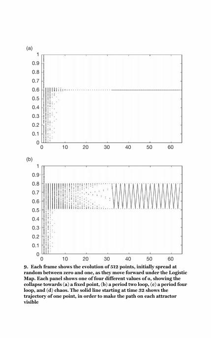
9. Each frame shows the evolution of 512 points, initially spread atrandom between zero and one, as they move forward under the LogisticMap. Each panel shows one of four different values of α, showing thecollapse towards (a) a fixed point, (b) a period two loop, (c) a period fourloop, and (d) chaos. The solid line starting at time 32 shows thetrajectory of one point, in order to make the path on each attractorvisible

dynamical system with fixed equations (structure) and specified

parameter values, so the uncertainty that chaos acts on is only

the uncertainty in the initial state. In practice, these distinctions

become blurred and the situation is much more interesting, and

confused.

Statistical models of Sun spots

Chaos is only found in deterministic systems. But to understand its

impact on science we need to view it against the background of

traditional stochastic models developed over the past century.

Whenever we see something repetitive in nature, periodic motion

is one of the first hypotheses to be deployed. It can make you

famous: Halley’s comet, and the Wolf Sun spot number. In the

end, the name often sticks even when we realize that the

phenomenon is not really periodic. Wolf guessed that the Sun

went through a cycle of about 11 years at a time when he had less

than 20 years’ data. Periodicity remains a useful concept even

though it is impossible to prove a physical system is periodic

regardless of how much data we take. So are the concepts of

determinism and chaos.

The solar record showed correlations with weather, with economic

activity, with human behaviour; even 100 years ago the 11-year

cycle could be ‘seen’ in tree rings. How could we model the Sun

spots cycle? Models of a frictionless pendulum are perfectly

periodic, while the solar cycle is not. In the 1920s, the Scottish

statistician Udny Yule discovered a new model structure, realizing

how to introduce randomness into the model and get more

realistic-looking time series behaviour. He likened the observed

time series of Sun spots to those from the model of a damped

pendulum, a pendulum with friction which would have a free

period of about 11 years. If this model pendulum were ‘left alone

in a quiet room’, the resulting time series would slowly damp down

to nothing. In order to motivate his introduction of random

numbers to keep the mathematical model going, Yule extended the

50

Ch

ao

s

analogy with a physical pendulum: ‘Unfortunately, boys with pea

shooters get into the room, and pelt the pendulum from all sides at

random.’ The resulting models became a mainstay in the

statistician’s arsenal. A linear, stochastic mainstay. We will define

the Yule Map:

Take α times X plus a random value R to be the new value of X

where R is randomly drawn from the standard bell-shaped

distribution.

So how does this stochastic model differ from a chaotic model?

There are two differences that immediately jump out at the

mathematician: the first is that Yule’s model is stochastic – the

rule requires a random number generator, while a chaotic model

of the Sun spots would be deterministic by definition. The second

is that Yule’s model is linear. This implies more than simply that

we do not multiply components of the state together in the

definition of the map; it also implies that one can combine

solutions of the system and get other acceptable solutions, a

property called superposition. This very useful property is not

present in nonlinear systems.

Yule developed a model similar to the Yule Map that behaved more

like the time series of real Sun spots. Cycles in Yule’s improved

model differ slightly from one cycle to the next due to the random

effects, the details of the pea shooters. In a chaotic model the state

of the Sun differs from one cycle to the next. What about

predictability? In any chaotic model, almost all nearby initial

states will eventually diverge, while in each of Yule’s models even far

away initial states would converge, if both experienced the same

forcing from the pea shooters. This is an interesting and rather

fundamental difference: similar states diverge under deterministic

dynamics whereas they converge under linear stochastic dynamics.

That does not necessarily make Yule’s model easier to forecast, since

we never know the details of the future random forcing, but it

changes the way that uncertainty evolves in the system, as shown in

51

Ch

ao

s in co

nte

xt: d

ete

rmin

ism, ra

nd

om

ne

ss, an

d n

oise

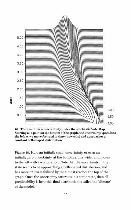
Figure 10. Here an initially small uncertainty, or even an

initially zero uncertainty, at the bottom grows wider and moves

to the left with each iteration. Note that the uncertainty in the

state seems to be approaching a bell-shaped distribution, and

has more or less stabilized by the time it reaches the top of the

graph. Once the uncertainty saturates in a static state, then all

predictability is lost; this final distribution is called the ‘climate’

of the model.

10. The evolution of uncertainty under the stochastic Yule Map.Starting as a point at the bottom of the graph, the uncertainty spreads tothe left as we move forward in time (upwards) and approaches aconstant bell-shaped distribution

52

Ch

ao

s

Physical dynamical systems

There is no way of proving the correctness of the position of

‘determinism’ or ‘indeterminism’. Only if science were complete or

demonstrably impossible could we decide such questions.

E. Mach (1905)

There is more to the world than mathematical models. Just about

anything we want to measure in the real world, or even just think

about observing, can be taken to have come from a physical

dynamical system. It could be the position of the planets in the solar

system, or the surface of a cup of coffee on a vibrating table, or the

population of fish in a lake, or the number of grouse on an estate, or

a coin being flipped.

The time series we want to observe now is the state of the physical

system: say, the position of our nine planets relative to the Sun, the

number of fish or grouse. As a short-hand, we will again denote the

state of the system as X, while trying to remember that there is a

fundamental difference between a model-state and the True state, if

such a thing exists. It is unclear how these concepts stand in

relation to each other; as we shall see in Chapter 11, some

philosophers have argued that the discovery of chaos implies the

real world must have special mathematical properties. Other

philosophers, perhaps sometimes the same ones, have argued that

the discovery of chaos implies mathematics does not describe the

world. Such are philosophers.

In any event, we never have access to the True state of a physical

system, even if one exists. What we do have are observations,

which we will call ‘S’ to distinguish them from the state of the

system, X. What is the difference between X and S? The unsung

hero of science: noise. Noise is the glue that bonds the

experimentalists with the theorists on those occasions when they

meet. Noise is also the grease that allows theories to slide easily

over awkward facts.

53

Ch

ao

s in co

nte

xt: d

ete

rmin

ism, ra

nd

om

ne

ss, an

d n

oise

In the happy situation where we know the mathematical model

which generated the observations and we also know of a noise

model for whatever generated whatever noise there was, then we

are in the Perfect Model Scenario, or PMS. It is useful to

distinguish a strong version of PMS where we know the parameter

values exactly, from a weak version where we know only the

mathematical forms and must estimate parameter values from the

observations. As long as we are in either version of PMS, the noise is

defined by the distance between X and S, and it makes sense to

speak of noise as causing our uncertainty in the state, since we know

a True state exists even if we do not know its value. Not much of this

picture survives when we leave PMS. Even within PMS, noise takes

on a new prominence once we acknowledge that the world is not

linear.

What about the concepts of deterministic and random, or even

periodic? These refer to properties of our models; we can apply

them to the real world only via (today’s) best model. Are there really

random physical dynamical systems? Despite the everyday use of

coin flips and dice as sources of ‘randomness’, the typical answer in

classical physics is: no, there is no randomness at all. With a

complete set of laws it may (or may not) be too difficult for us to

calculate the outcomes of coin flips, rolling dice, or spinning a

roulette: but that is a problem only in practice, not in principle:

Laplace’s demon would have no difficulty with such predictions.

Quantum mechanics, however, is different. Within the traditional

quantum mechanical theory, the half-life of a uranium atom is as

natural and real a quantity as the mass of the uranium atom. The

fact that classical coin tosses or roulette are not best modelled as

random is irrelevant, given the quantum mechanical claim for

randomness and objective probabilities. Claims for – or against –

the existence of objective probabilities require interpreting physical

systems in terms of our models of those systems. As always. Some

future theory may revoke this randomness in favour of

determinism, but we are on the scene only for a vanishingly

small interval. It is relatively safe to say that some of our best

54

Ch

ao

s

models of reality will still admit random elements as you read these

words.

Observations and noise

Over the last few decades, a huge number of scientific papers have

been written about using a time series to distinguish deterministic

systems from stochastic systems. This avalanche was initiated in the

physics literature, and then spread into geophysics, economics,

medicine, sociology, and beyond. Most of these papers were

inspired by a beautiful theorem proven by the Dutch

mathematician Floris Takens in 1983, to which we will return in

Chapter 8. Why were all these papers written, given that we have a

simple rule for determining if a mathematical system is

deterministic or stochastic? Why not just look at the rules of the

system and see if it requires a random number generator? It is

common to confuse the games mathematicians play with

constraints placed on the work of the natural (and other) scientists.

Real mathematicians like to play intellectual games, like pretending

to forget the rules and then guessing if the system is deterministic

or stochastic from looking only at the time series of the states of the

system. Could they clearly identify any deterministic system given

the time series from the infinitely remote past to the infinitely

distant future? For fixed points and even periodic loops, this game

is not challenging enough; to make it more interesting, consider a

variation in which we do not know the exact states, but have access

only to noisy observations, S, of each state X. The origin S is

commonly, if somewhat misleadingly, thought of as being related to

the addition of a random number to each true X. In that case, this

observational noise does not affect the future states of the system,

only our observations of each state; it is a very different role from

that played by the random numbers R in the stochastic systems, like

the Yule Map where the value of R did impact the future since it

changed the next value of X. To maintain this distinction, random

influences that do influence X are called dynamic noise.

55

Ch

ao

s in co

nte

xt: d

ete

rmin

ism, ra

nd

om

ne

ss, an

d n

oise

As noted above, mathematicians can work within the Perfect Model

Scenario (PMS). They start off knowing that the model which

generated the time series has a certain kind of structure, and

sometimes they assume they know the structure (weak PMS),

sometimes even the values of the parameters as well (strong PMS).

They generate a time series of X, and from this a time series of S.

They then pretend to forget the values of X and see if they can work

out what they were, or they pretend to forget the mathematical

system and see if, given only S, they can identify the system along

with its parameter values, or determine if the system is chaotic, or

forecast the next value of X.

At this point, it should be pretty easy to see where their game is

going: our mathematicians are trying to simulate the situation that

natural scientists can never escape from. The physicists, earth

scientists, economists, and other scientists do not know the rule, the

full Laws of Nature, relevant to the physical systems of scientific

study. And scientific observations are not perfect; they may be

invariably uncertain due to observational noise, but that is not the

end of the story. It is a capital mistake to confuse real observations

with those of these mathematical games.

The natural scientist is forced to play a different game. While

attempting to answer the same questions, the scientist is given only

a time series of observations, S, some information regarding the

statistics of the observational noise, and the hope that some

mathematical map exists. Physicists can never be sure if such a

structure exists or not; they cannot even be certain if the model

state variable X really has any physical meaning. If X is the number

of rabbits in a real garden, it is hard to imagine that X does not

exist, it is just some whole number. But what about model variables

like wind speed or temperature? Are there real numbers that

correspond to those components of our state vector? And if not,

where between rabbits and wind speed does the correspondence

break down?

56

Ch

ao

s

Our philosopher is very interested in such questions, and we all

should be. LeVerrier, the Frenchman who worked with Fitzroy to

set up the first weather warning system, died famous for discovering

two planets. He used Newton’s Laws to predict the location of

Neptune based on ‘irregularities’ in the observed time series of

Uranus’s orbit, and that planet was duly observed. He also analysed

‘irregularities’ in the orbit of Mercury, and again told observers

where to find another new planet. And they did: the new planet,

named Vulcan, was very near the Sun and difficult to see, but it was

observed for decades. We now know that there is no planet Vulcan;

LeVerrier was misled because Mercury’s orbit is poorly described by

Newton’s Laws (although it is rather better described by Einstein’s).

How frequently do we blame the mismatch between our models

and our data on noise when the root cause is in fact model

inadequacy? Most really interesting science is done at the edges,

whether the scientists realize it or not. We are never sure if today’s

laws apply there or not. Modern-day climate science is a good

example of hard work being done at the edge of our understanding.

The study of chaos has clarified the importance of distinguishing

two different issues: one being the effects of uncertainty in the state

or the parameters, the other being the inadequacy of our

mathematics itself. Mathematicians working within PMS can make

progress by pretending that they are not, while scientists who

pretend – or believe – that they are working within PMS when they

are not can wreak havoc, especially if their models are naıvely taken

as a basis for decision making. The simple fact is that we cannot

apply the standards of mathematical proof to physical systems, but

only to our mathematical models of physical systems. It is

impossible to prove that a physical system is chaotic, or to prove it is

periodic. Our physicist and mathematician must not forget that

they sometimes use the same words to mean rather different things;

when they do, they often run into some difficulty and considerable

acrimony. Mach’s comment above (page 53) suggests that this is not

a new issue.

57

Ch

ao

s in co

nte

xt: d

ete

rmin

ism, ra

nd

om

ne

ss, an

d n

oise

Chapter 4

Chaos in mathematical

models

We would all be better off if more people realised that simple nonlinear

systems do not necessarily possess simple dynamical properties.

Lord May (1976)

This chapter consists of a very short survey of chaotic mathematical

models from zoology to astronomy. Like any cultural invasion, the

arrival of nonlinear deterministic models with sensitive dependence

was sometimes embraced, and sometimes not. It has been most

uniformly welcomed in physics where, as we shall see, the

experimental verification of its prophecies has been nothing short of

astounding. In other fields, including population biology, the very

relevance of chaos is still questioned. Yet it was population

biologists who proposed some of the first chaotic models a decade

before the models of astronomers and meteorologists came on the

scene. Renewed interest in this work was stimulated in 1976 by an

influential and accessible review article in the journal Nature. We

begin with the basic insights noted in that article.

The darling bugs of May

In 1976, Lord May provided a high-profile review of chaotic

dynamics in Nature that surveyed the main features of

deterministic nonlinear systems. Noting that many interesting

questions remained unresolved, he argued that this new perspective

58

provided not just theoretical but practical and pedagogical value as

well, and that it suggested everything from new metaphors for

describing systems to new quantities to observe and new parameter

values to estimate. Some of the simplest population dynamics are

those of breeding populations when one generation does not

overlap with the next. Insects that have one generation per year, for

example, might be described by discrete time maps. In this case Xi

would represent the population, or population density, in the ith

year, so our time series would have one value per year, and the map

is the rule that determines the size of next year’s population given

this year’s. A parameter α represents the density of resources. In the

1950s, Moran and Ricker independently suggested the map shown

in Figure 8(f ) (page 40). Looking at this graph, we can see that

when the current value of X is small, the next value of X is larger:

small populations grow. Yet if X gets too big, then the next value of

X is small, and when the current value is very large, the next value is

very small: large populations exhaust the resources available to each

individual, and so successful reproduction is reduced.

Irregularly fluctuating populations have long been observed, and

researchers have long argued over their origin. Time series of

Canadian lynx and both Scandinavian and Japanese voles are, along

with the Sun spot series, some of the most analysed data sets in all

of statistics. The idea that very simple nonlinear models can display

such irregular fluctuations suggested a new potential mechanism

for real population fluctuations, a mechanism that was in conflict

with the idea that ‘natural’ populations should maintain either a

steady level or a regular periodic cycle. The idea that these random-

looking fluctuations need not be induced by some outside force like

the weather, but could be inherent to the natural population

dynamics, had the potential to radically alter attempts to

understand and manage populations. While noting that ‘replacing a

population’s interactions with its biological and physical

environment by passive parameters may do great violence to the

reality’, May provided a survey of interesting behaviours in the

Logistic Map. The article ends with ‘an evangelical plea for the

59

Ch

ao

s in m

ath

em

atica

l mo

de

ls

introduction of these difference equations into elementary

mathematics courses, so that students’ intuition may be enriched by

seeing the wild things that simple nonlinear equations can do’. That

was three decades ago.

We will consider a few of these wild things below, but note that the

mathematicians’ focus on the Logistic Map is not meant to suggest

that this map itself in any sense ‘governs’ the various physical and

biological systems. One thing that distinguishes nonlinear

dynamics from traditional analysis is that the former tends to focus

more on the behaviour of systems rather than on the details of any

one initial state under particular equations with specific parameter

values: a focus on geometry rather than statistics. Similar dynamics

can be more important than ‘good’ statistics. And it turns out that

the Logistic Map and the Moran-Ricker Map are very similar in this

way, even though they look very different in Figure 8(f ) (page 40).

The details may well matter, of course; the enduring role of the

Logistic Map itself may be pedagogical, helping to exorcize the

historical belief that complicated dynamics requires either very

complicated models or randomness.

Universality: prophesying routes to chaos

The Logistic Map gives rise to amazingly rich varieties of behaviour.

The famous bifurcation diagram of Figure 11 summarizes the

behaviour of the map at many different values of its parameter in

one figure. The horizontal axis is α and the dots in any vertical slice

indicate states which fall near the attractor for that value of α. Here

α reflects some parameter of the system: if X is the number of fish in

the lake, then α is the amount of food in the lake; if X is the time

between drips of the faucet, then α is the rate of water leaking

through the tap; if X is the motion of rolls in fluid convection, then

α is the heat delivered to the bottom of the pan. In models of very

different things, the behaviour is the same. For small α (on the left)

we have a fixed point attractor. The location of the fixed point

increases as α increases, until α reaches a value of one, where the

60

Ch

ao

s

fixed point vanishes and we observe iterations which alternate

between two points: a period two loop. As α continues to increase,

we get a period four loop, then period eight, then 16, then 32. And

so on. Bifurcating over, and over again.

Since the period of the loop always increases by a factor of two, these

are called period doubling bifurcations. While the old loops are no

longer seen, they do not cease to exist. They are still there, but have

become unstable. This is what happened to the origin in the Logistic

Map when α is greater than one: X only stays at zero if it is exactly

equal to zero, while small non-zero values grow at each iteration.

Similarly, points near an unstable periodic loop move away from it,

and so we no longer see them clearly when iterating the map.

There is a regularity hidden in Figure 11. Take any three consecutive

values of α at which the period doubles, subtract the first from the

second, and then divide that number by the difference between the

second and the third. The result leads to the Feigenbaum number,

~4.6692016091. Mitch Feigenbaum discovered these relationships,

working with a hand calculator in Los Alamos in the late 1970s, and

11. Period doubling behaviour in the Logistic Map as α increases from2.8 to ~3.5; the first three doublings are marked

61

Ch

ao

s in m

ath

em

atica

l mo

de

ls

the ratio is now known by his name. Others also found it

independently; having the insight to do this calculation was

stunning in each case.

Since the Feigenbaum number is greater than one, values of α at

which bifurcations occur get closer and closer together, and we have

an infinite number of birfurcations before reaching a value of α near

3.5699456718. Figure 12 indicates what happens for larger values

of α. This sea of points is largely chaotic. But note the windows of

periodic behaviour, for instance the period three window where α

takes on the value of one plus the square root of eight (that is, about

3.828). This is a stable period three loop; can you identify windows

corresponding to period five? Seven?

Figure 13 puts the figures of the Logistic Map in context. Randomly

chosen values for α and X0 form a cloud of points on the t equals

zero slice of this three-dimensional figure. Iterating the Logistic

Map forward from these values, the transients fall away, and the

attractors at each value of α slowly come into view, so that after 512

iterations the last time slice resembles Figure 12.

12. A variety of behaviours in the Logistic Map as α increases from aperiod four loop at α = 3.5 to chaos at α = 4. Note the replicated perioddoubling cascades at the right side of each periodic window

62

Ch

ao

s

13. Three-dimensional diagram showing the collapse of initially random values of X0 and α at the left rear side of the boxfalling toward their various attractors as the number of iterations increases. Note the similarity of the points near the rightforward side with those in Figures 11 and 12

It would be asking too much to expect something as simple as the

Logistic Map to tell us anything about the behaviour of liquid

helium. But it does. Not only does the onset of complicated

behaviour show a qualitative indication of period doubling, the

actual quantitative values of the Feigenbaum numbers computed

from many experiments agree remarkably well with those

computed from the Logistic Map. Many physical systems seem to

display this ‘period doubling route to chaos’: hydrodynamics (water,

mercury, and liquid helium), lasers, electronics (diodes,

transistors), and chemical reactions (BZ reaction). One can often

estimate the Feigenbaum number to two-digits’ accuracy in

experiments. This is one of the most astounding results reported in

this Introduction to chaos: how could it be that simple calculations

with the Logistic Map can give us information that is relevant to all

these physical systems?

The mathematician’s fascination with this diagram arises not only

from its beauty but also from the fact that we would get a similar

picture for the Moran-Ricker Map and many other systems that at

first instance appear quite different from the Logistic Map. A

technical argument shows that the period doubling is common in

‘one-hump’ maps where the hump looks like a parabola. In a very

real and relevant sense, almost all nonlinear maps look like this very

close to their maximum value, so properties like period doubling

are called ‘universal’, although not all maps have them. More

impressive than these mathematical facts is the empirical fact that a

wide variety of physical systems display unexpected behaviour that,

as far as we can see, reflects this mathematical structure. Is this not

then a strong argument for the mathematics to govern, not merely

describe, Nature? To address this question, we might consider

whether the Feigenbaum number is more akin to a constant of

geometry, like π, or a physical constant like the speed of light, c. The

geometry of disks, cans, and balls is well described using π, but π

hardly governs the relationship between real lengths, area, and

volumes in the same way that the values of physical constants

govern the nature of things within our laws of nature.

64

Ch

ao

s

The origin of the mathematical term ‘chaos’

In 1964 the Russian mathematician A. N. Sharkovski proved a

remarkable theorem about the behaviours of many ‘one-hump’

maps: namely that discovering a periodic loop indicated that others,

potentially lots of others, existed. Discovering that a period 16 loop

existed for a particular value of the parameter implied there were

loops of period eight and of four and of two and of one at that value;

while finding a loop of period three meant that there was a loop of

every possible period! It is another non-constructive proof; it does

not tell us where those loops are, but nevertheless it is a pretty neat

result. Eleven years after Sharkovski, Li and Yorke published their

enormously influential paper with the wonderful title ‘Period Three

Implies Chaos’. The name ‘chaos’ stuck.

Higher-dimensional mathematical systems

Most of our model states so far have consisted of just one

component. The vole and weasel model is an exception, since the

state consisted of two numbers: one reflecting the population of

voles, the other the population of weasels. In this case, the state is a

vector. Mathematicians call the number of components in the state

the dimension of the system, since plotting the state vectors would

require a state space of that dimension.

As we move to higher dimensions, the systems are often not maps

but flows: a map is a function that takes one value of X and returns

the next value of X, while a flow provides the velocity of X for any

point in the state space. Think of a parsnip floating under the

surface of the sea; it is carried along by the current and will trace

out the flow of the sea. The three-dimensional path of the parsnip in

the sea is analogous to a path traced out by X in the state space, and

both are sometimes called trajectories. If instead of a parsnip, we

follow the path of an infinitesimal parcel of the fluid itself, we often

find these paths to be recurrent with sensitive dependence. The

equations are deterministic and these fluid parcels are said to

65

Ch

ao

s in m

ath

em

atica

l mo

de

ls

display ‘Lagrangian chaos’. Laboratory experiments with fluids

often display beautiful patterns which reflect the chaotic dynamics

observed in our models of fluid flow. Without examining the

differential equations that define these velocity fields, we will next

touch several classic chaotic systems.

Dissipative chaos

In 1963, Ed Lorenz published what became a classic paper on the

predictability of chaotic systems. He considered a vastly simplified

set of three equations based on the dynamics of a fluid near the

onset of convection which is now called the Lorenz System. One can

picture the three components of the state in terms of convective

rolls in a layer of fluid between two flat plates when the lower plate

is heated. When there is no convection, the fluid is motionless and

the temperature in the fluid decreases uniformly from the warmer

plate at the bottom to the cooler plate at the top. The state X of the

Lorenz model consisted of three values {x,y,z}, where x reflected the

speed of the rotating fluid, y quantified the temperature difference

between rising and sinking fluid, and z measured the deviation

from the linear temperature profile. An attractor from this system is

shown in Figure 14; by chance, it looks something like a butterfly.

The different shading on the attractor indicates variations in the

time it takes an infinitesimal uncertainty to double. We return to

discuss the meaning of these shades in Chapter 6, but note the

variations with location.

The evolution of uncertainty in the Lorenz system is shown in

Figure 15; this looks a bit more complicated than the corresponding

figure for the Yule Map in Figure 10 (page 52). Figure 15 shows the

kind of forecast our 21st-century demon could make for this system:

an initial small uncertainty at the bottom of the panel grows wider,

then narrower, then wider, then narrower . . . eventually splitting

into two parts and beginning to fade away. But depending on the

decisions we are trying to make, there may still be useful

information in this pattern even at the time reflected at the top of

66

Ch

ao

s

14. Three-dimensional plots of (above) the Lorenz attractor and(below) the Moore-Spiegel attractor. The shading indicates variationsin uncertainty doubling time at each point

15. The probability forecast our 21st-century demon would make forthe 1963 Lorenz System. Contrast the way uncertainty evolves in thischaotic system with the relatively simple growth of uncertainty underthe Yule Map shown in Figure 10 on page 52

the panel. On this occasion the uncertainty has not stabilized by the

time it reaches the top of the graph.

In 1965, mathematical astronomers Moore and Spiegel considered

a simple model of a parcel of gas in the atmosphere of a star. The

state space is again three-dimensional, and the three components of

X are simply the height, velocity, and acceleration of the parcel. The

dynamics are interesting because we have two competing forces: a

thermal force that tends to destabilize the parcel and a magnetic

force that tends to bring it back to its starting point, much like a

spring would. As the parcel rises, it finds itself at a different

temperature than the surrounding fluid and this feeds back on its

velocity and its temperature, but at the same time the star’s

magnetic field acts as a spring to pull the parcel back towards its

original location. Motion caused by two competing forces often

gives rise to chaos. The Moore-Spiegel attractor is also shown in

Figure 16.

Chaos experiments have always pushed computers to their limits,

and sometimes slightly beyond those limits. In the 1970s, the

astronomer Michael Hénon wanted to make a detailed study of

chaotic attractors. For a given amount of computer power there

is a direct trade-off between the complexity of the system and

the duration of the time series one can afford to compute.

Hénon wanted a system with properties similar to Lorenz’s

1963 system that would be cheaper to iterate on his computer.

This was a two-dimensional system, where the state X consisted

of the pair of values {x,y}. The Hénon Map is defined by the

rules:

The new value of x i + 1 is equal to one minus yi plus α times xi2;

the new value of y i + 1 is equal to β times xi.

Panel (b) of Figure 16 shows the attractor when α is 1.4 and β is 0.3;

panel (a) shows a slice of the Moore-Spiegel attractor made by

combining snapshots of the system whenever z was zero and

69

Ch

ao

s in m

ath

em

atica

l mo

de

ls

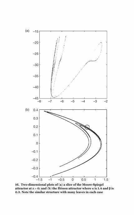
16. Two-dimensional plots of (a) a slice of the Moore-Spiegelattractor at z = 0; and (b) the Hénon attractor where α is 1.4 and β is0.3. Note the similar structure with many leaves in each case

growing. This type of figure is called a Poincaré section and

illustrates how slices of a flow are much like maps.

Delay equations, epidemics, and medicaldiagnostics

Another interesting family of models are delay equations. Here both

the current state and some state in the past (the ‘delayed state’) play

a direct role in the dynamics. These models are common for

biological systems, and can provide insight into oscillatory diseases

like leukaemia. In the blood supply, the number of cells available

tomorrow depends upon the number available today, and also the

number of new cells that mature today; the delay comes from the

gap in time between when these new cells are requested and when

they mature: the number of cells maturing today depends on the

number of blood cells at some point in the past. There are many

other diseases with this kind of oscillatory dynamics, and the study

of chaos in delay equations is extremely interesting and productive.

We leave the discussion of mathematical models for a paragraph to

note that medical research is another area where insights from our

mathematical models are deployed for use in real systems. Research

by Mike Mackey at McGill University and others on delay equations

has even led to a cure for at least one oscillatory disease. The study

of nonlinear dynamics has also led to insights in the evolution of

diseases that oscillate in a population, not an individual; our models

can be contrasted with reality in the study of measles, where one

can profitably consider the dynamics in time and in space. The

analysis of chaotic time series has also led to the development of

insightful ways to view complicated medical time series, including

those from the brain (EEG) and heart (ECG). This is not to suggest

that these medical phenomena of the real word are chaotic, or even

best described with chaotic models; methods of analysis developed

for chaos may prove of value in practice regardless of the nature of

the underlying dynamics of the real systems that generate the

signals analysed.

71

Ch

ao

s in m

ath

em

atica

l mo

de

ls

Hamiltonian chaos

If volumes in state space do not shrink in time there can be no

attractors. In 1964, Hénon and Heiles published a paper showing

chaotic dynamics in a four-dimensional model of the motion of a

star within a galaxy. Systems in which volumes in state space do not

shrink, including those of Newtonian celestial mechanics commonly

used to predict eclipses, and which trace the future of the solar

system and spacecraft within it, are called Hamiltonian. Figure 17

is a slice from the Hénon-Heiles system, which is Hamiltonian.

Note the intricate interweaving of empty islands in a sea of chaotic

trajectories. Initial states started within these islands may fall onto

almost closed loops (tori); alternatively they may follow chaotic

trajectories confined within an island chain. In both cases, the order

in which the islands in the chain are visited is predictable, although

exactly where on each island might be unpredictable; in any case,

things are only unpredictable on small length scales.

17. A two-dimensional slice of the Hénon-Heiles attractor. Note thesimultaneous loops, and a chaotic sea with many (empty) islands

72

Ch

ao

s

Exploiting the insights of chaos

In the three-year period between 1963 and 1965, three

independent papers appeared (by Lorenz, by Moore and Spiegel,

and by Hénon and Heiles), each using digital computers to

introduce what would be called ‘chaotic dynamics’. In Japan, chaos

had been observed in analogue computer experiments by

Yoshisuke Ueda, and Russian mathematicians were advancing

upon a groundwork laid down by over a century of international

mathematics. Almost 50 years later, we are still finding new ways

to exploit these insights.

What limits the predictability of future solar eclipses? Is it

uncertainty in our knowledge of the planetary orbits due to

the limited accuracy of our current measurements? Or future

variations in the length of the day which alters the point on the

surface of the Earth under the eclipse? Or the failure of

Newton’s equations due to effects (better) described by general

relativity? We can see that the Moon is slowly moving away

from the Earth, and assuming that this continues, it will

eventually appear too small to block the entire Sun. In that

case, there will be a last total eclipse of the Sun. Can we

forecast when that event will occur and, weather permitting,

where we should be on the surface of the Earth in order to

see it? We do not know the answer to that question. Nor do we

know, for certain, if the solar system is stable. Newton was well

aware of the difficulties nonlinearities posed for determining

the ultimate stability of only three celestial bodies, and

suggested that insuring the stability of the solar system was a

task for God. By understanding the kinds of chaotic orbits

that Hamiltonian systems admit, we have learned many things

about the ultimate stability of the solar system. Our best guess,

currently, is that our solar system is stable, probably. Insights

like these come from understanding the geometry in state space

rather than attempting detailed calculations based upon

observations.

73

Ch

ao

s in m

ath

em

atica

l mo

de

ls

Can we safely draw insights from mathematical behaviour of

low-dimensional systems? They suggest new phenomena to look

for in experiments, like periodic doubling, or suggest new

constants to estimate in Nature, like the Feigenbaum number.

These simple systems also provide test beds for our forecast

methods; this is a bit more dangerous. Are the phenomena of

low-dimensional chaotic systems the same phenomena that we

observe in more complicated models? Are they so common that

they occur even in simple low-dimensional systems like Lorenz

1963 or the Moore-Spiegel system? Or are these phenomena

due to the simplicity of these examples: do they occur only in

simple mathematical systems? The same even in or only in

question applies to techniques developed to forecast or control

chaotic systems, which are tested in low-dimensional systems:

do these things happen even in or only in low-dimensional

systems? The most robust answer so far is that difficulties

we identify in low-dimensional systems rarely go away in

higher-dimensional systems, while successful solutions to

these difficulties which work in low-dimensional systems

often fail to work in higher-dimensional systems. Recognizing

the danger of generalizing from three-dimensional systems,

Lorenz moved on to a 28-dimensional system about 50 years ago;

he is still creating new systems today, some in two dimensions and

others in 200 dimensions.

Chaos and nonlinearity impact many fields; perhaps the deepest

insight to be drawn here is that complicated-looking solutions are

sometimes acceptable and need not be due to external dynamic

noise. This does not imply that, in any particular case, they are not

due to external noise, nor does it lessen the practical value of

stochastic statistical modelling, which has almost a century of

experience and statistical good practice behind it. It does suggest

the value in developing tests for which methods to use in a given

application, and consistency tests for all modelling approached.

Our models should be as uninhibited as possible, but not more so.

The lasting impact of these simple systems may be in their

74

Ch

ao

s

pedagogical value; young people can be exposed to the rich

behaviours of these simple systems early in their education. By

requiring internal consistency, mathematics constrains our flights

of fancy in drawing metaphors, not so much as to bring them in line

with physical reality, but often opening new doors.

75

Ch

ao

s in m

ath

em

atica

l mo

de

ls

Chapter 5

Fractals, strange attractors,

and dimension(s)

Big fleas have little fleas

upon their backs to bite’em.

And little fleas have lesser fleas,

and so ad infinitum.

A. de Morgan (1872)

No introduction to chaos would be complete without touching upon

fractals. This is neither because chaos implies fractals nor because

fractals require chaos, but simply because in dissipative chaos real

mathematical fractals appear as if from nowhere. It is just as

important to distinguish mathematical fractals from physical

fractals as it is to distinguish what we mean by chaos in

mathematical systems from what we mean by chaos in physical

systems. Despite decades of discussion, there is no single generally

accepted definition of a fractal in either case, although you can

usually recognize one when you see it. The notion is bound up in

self-similarity: as we zoom in on the boundary of clouds, countries,

or coastlines, we see patterns similar to those seen at the larger-

length scales again and again. The same thing happens with the set

of points in Figure 18. Here the set is composed of five clusters of

points; if we enlarge any one of these clusters, we find the

enlargement looks similar to the entire set itself. If this similarity is

exact – if the zoom is equivalent to the original set – then the set is

called strictly self-similar. If only statistical properties of interest

76

are repeated, then the set is called statistically self-similar.

Deciding exactly what counts as a ‘statistical property of interest’

opens one of the discussions that has prevented agreement on a

general definition. Disentangling these interesting details deserves

its own Very Short Introduction to Fractals; we will content

ourselves with some examples.

In the late 18th century, fractals were widely discussed by

mathematicians including Georg Cantor, although the famous

Middle Thirds set that bears his name was first found by an Oxford

mathematician named Henry Smith. Fractal entities were often

disavowed by their mathematical parents as monstrous curves in

the 100 years that followed, just as L. F. Richardson was beginning

to quantify the fractal nature of various physical fractals. Both

physical and mathematical fractals were more warmly embraced by

astronomers, meteorologists, and social scientists. One of the first

fractals to bridge the divide – and blur the distinction – between a

mathematical space and real-world space appeared about 100 years

ago in an attempt to resolve Olbers’ paradox.

A fractal solution to Olbers’ paradox

In 1823, the German astronomer Heinrich Olbers encapsulated a

centuries-old concern of astronomers in the concise question: ‘Why

is the night sky dark?’ If the universe were infinitely large and more

or less uniformly filled with stars, then there would be a balance

between the number of stars at a given distance and the light we get

from each one of them. This delicate balance implies that the night

sky should be uniformly bright; it would even be difficult to see the

Sun against a similarly bright day-time sky. But the night sky is

dark. That is Olbers’ paradox. Johannes Kepler used this as an

argument for a finite number of stars in 1610. Edgar Allan Poe was

the first to suggest an argument still in vogue today: that the night

sky was dark because there had not been enough time for light from

far-away stars to reach the Earth, yet. Writing in 1907, Fournier

d’Albe proposed an elegant alternative, suggesting that the

77

Fracta

ls, stran

ge

attra

ctors, a

nd

dim

en

sion

(s)

distribution of matter in the universe was uniform but in a fractal

manner. Fournier illustrated his proposal with the figure

reproduced in Figure 18. This set is called the Fournier Universe. It

is strictly self-similar: blowing up one of the small cubes by a factor

of 5 yields an exact duplicate of the original set. Each small cube

contains the totality of the whole.

The Fournier Universe illustrates a way out of Olbers’ paradox: the

line Fournier placed in Figure 18 indicates one of many directions

in which no other ‘star’ will ever be found. Fournier did not stop

18. The Fournier Universe, showing the self-similar structure, aspublished by Fournier himself in 1907

78

Ch

ao

s

at the infinitely large, but also suggested that this cascade

actually extended to the infinitely small; he interpreted atoms as

micro-verses, which were in turn made of yet smaller particles, and

suggested macro-verses in which our galaxies would play the role of

atoms. In this way, he proposed one of the few physical fractals with

no inner cut-off and no outer cut-off: a cascade that went from the

infinitely large to the infinitesimally small in a manner reminiscent

of the last frames of the film Men in Black.

Fractals in physics

Big whorls have little whirls,

which feed on their velocity.

And little whirls have lesser whirls,

and so on to viscosity.

L. F. Richardson

Clouds, mountains, and coastlines are common examples of

natural fractals; statistically self-similar objects that exist in real

space. Interest in generating fractal irregularity is not new:

Newton himself recorded an early recipe, noting that when beer

is poured into milk and ‘the mixture let stand till dry, the surface

of the curdled substance will appear as rugged and mountainous

as the earth at any place’. Unlike Newton’s curdled substance, the

fractals of chaos are mathematical objects found in state spaces;

they are true fractals as opposed to their physical counterparts.

What is the difference? Well, for one thing, a physical fractal only

displays the properties of a fractal at certain length scales and not

at others. Consider the edge of a cloud: as you look more and

more closely, going to smaller and smaller length scales, you’ll

reach a point at which the boundary is no more; the cloud

vanishes into the helter-skelter rush of molecules and there is no

boundary to measure. Similarly, a cloud is not self-similar on

length scales comparable with the size of the Earth. For physical

fractals, fractal concepts break down as we look too closely; these

physical cut-offs make it easy to identify old Hollywood special

79

Fracta

ls, stran

ge

attra

ctors, a

nd

dim

en

sion

(s)

effects using model ships in wave tanks: we can sense the cut-off

is at the wrong length scale relative to the ‘ships’. Today, film

makers in Hollywood and in Wellington have learned enough

mathematics to generate computer counterfeits that hide the cut-

off better. The Japanese artist Hokusai respected this cut-off in

his famous ‘Great Wave’ print of the 1830s. Physicists have also

known this for some time: de Morgan’s poem allowed its cascade

of fleas to continue ad infinitum, while the cascade whorls in

L. F. Richardson’s version face a limit due to viscosity, the term

for friction within fluids. Richardson was expert in the theory

and observation of turbulence. He once threw parsnips off one

end of Cape Cod canal at regular intervals, using the time of their

arrival at a bridge on the other end of the canal to quantify how

the fluid dispersed as it moved downstream. He also computed

(by hand!) the first numerical weather forecast, during the First

World War.

A Quaker, who left the Met Office in the First World War to

become an ambulance driver in France, Richardson later became

interested in measuring the length of the border between nations

in order to test his theory that this influenced the likelihood of

their going to war. He identified an odd effect when measuring the

same border on different maps: the border between Spain and

Portugal was much longer when measured on the map of Portugal

than it was when measured on the map of Spain! Measuring

coastlines of island nations like Britain, he found that the length of

the coastline increased as the callipers he walked along the coast to

measure it decreased, and also noted an unexpected relationship

between the area of an island and its perimeter as both vary when

measured on different scales. Richardson demonstrated that these

variations with length scale followed a very regular pattern which

could be summarized by a single number for a particular

boundary: an exponent that related the length of a curve to the

length scale used to measure it. Following fundamental work by

Mandelbrot, this number is called the fractal dimension of the

boundary.

80

Ch

ao

s

Richardson developed a variety of methods to estimate the fractal

dimension of physical fractals. The area-perimeter method

quantifies how the area and perimeter both change under higher

and higher resolution. For one particular object, such as a single

cloud, this relationship also yields the fractal dimension of its

border. When we look at many different clouds at the same

resolution, as in a photograph from space, a similar relationship

between areas and perimeters emerges; we do not understand why

this alternative area-perimeter relation seems to hold for collections

of different-sized clouds, given that clouds are famous for not all

looking the same.

Fractals in state space

We next construct a rather artificial mathematical system

designed to dispel one of the most resilient and misleading

myths of chaos: that detecting upon a fractal set in state

space indicates deterministic dynamics. The Tripling Tent

Map is:

If X is less than a half then take 3X as the new value of X,

Otherwise take 3 minus 3X as the new value of X.

Almost every initial state between zero and one flies far away from

the origin; we will ignore these and focus on the infinite number of

initial conditions which remain forever between zero and one. (We

ignore the apparent paradox due to the loose use of ‘infinity’ here,

but note Newton’s warning that ‘the principle that all infinities are

equal is a precarious one’.)

The Tripling Tent Map is chaotic: it is clearly deterministic, the

trajectories of interest are recurrent, and the separation between

infinitesimally close points increases by a factor of three on each

iteration, which implies sensitive dependence. A time series from

the Tripling Tent Map, along with one from the stochastic Middle

Thirds IFS Map, are shown in Figure 19. Visually, we see hints that

81

Fracta

ls, stran

ge

attra

ctors, a

nd

dim

en

sion

(s)

19. A time series from (a) the stochastic Middle Thirds IFS Map and (b) the deterministic Tripling Tent Map. The lowerinsets show a summary of all the points visited: approximations to the Middle Thirds Cantor set in each case

the chaotic map is easier to forecast: small values of X are always

followed by small values of X The two small insets at the bottom of

Figure 19 each show a set of points visited by a long trajectory from

one of the systems, they look very similar and in fact both reflect

points from the Middle Thirds Cantor set. The two dynamical

systems each visit the same fractal set, so we can never distinguish

the deterministic system from the stochastic system if we only look

at the dimension of the set of points each system visits; but is it any

surprise that to understand the dynamics we have to examine how

the system moves about, not only where it has been? This simple

counter-example slays the myth noted above; while chaotic systems

may often move on fractal sets, detecting a finite dimensional set

indicates neither determinism nor chaotic dynamics.

Finding fractals in carefully crafted mathematical maps is not so

surprising, as mathematicians are clever enough to design maps

which create fractals. One of the neatest things about dissipative

chaos is that fractals appear without the benefit of intelligent

design. The Hénon Map is the classic example. Mathematically

speaking, it represents an entire class of interesting models; there is

nothing particularly ‘fractal-looking’ in its definition, as there is in

the Middle Thirds IFS Map. Figure 20 shows a series of zooms from

where, as if by magic, self-similar structures spring out. Surely this

is one of the most amazing things about nonlinear dynamical

systems. There is no hint of artificial design in the Hénon Map, and

fractal structure appears commonplace in the attractors of

dissipative chaotic systems. It is not required for chaos, nor vice

versa, but it is common.

Like all magic, we can understand how the trick works, at least after

the fact: we have chosen to zoom in about a fixed point of the

Hénon Map, and looking at the properties of the map very, very

close to this point reveals how much to zoom in order to make its

self-similarity so striking. The details of the repeated structure, a

thick line and two thinner lines, depend on what happens far away

from this point. But if Hénon is really chaotic and the computer

83

Fracta

ls, stran

ge

attra

ctors, a

nd

dim

en

sion

(s)

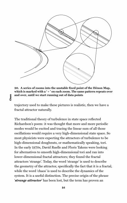
trajectory used to make these pictures is realistic, then we have a

fractal attractor naturally.

The traditional theory of turbulence in state space reflected

Richardson’s poem: it was thought that more and more periodic

modes would be excited and tracing the linear sum of all those

oscillations would require a very high-dimensional state space. So

most physicists were expecting the attractors of turbulence to be

high-dimensional doughnuts, or mathematically speaking, tori.

In the early 1970s, David Ruelle and Floris Takens were looking

for alternatives to smooth high-dimensional tori and ran into

lower-dimensional fractal attractors; they found the fractal

attractors ‘strange’. Today, the word ‘strange’ is used to describe

the geometry of the attractor, specifically the fact that it is a fractal,

while the word ‘chaos’ is used to describe the dynamics of the

system. It is a useful distinction. The precise origin of the phrase

‘strange attractor’ has been lost, but the term has proven an

20. A series of zooms into the unstable fixed point of the Hénon Map,which is marked with a ‘ + ’ on each zoom. The same pattern repeats overand over, until we start running out of data points

84

Ch

ao

s

inspiring and appropriate label for these objects of mathematical

physics. Since Hamiltonian systems have no attractors at all, they

have no strange attractors. Nevertheless, chaotic time series from

Hamiltonian systems often develop intricate patterns with stark

inhomogeneity and hints of self-similarity called strange

accumulators which persist for as long as we run our computers.

Their ultimate fate remains unknown.

Fractal dimensions

Counting the number of components in the state vector tells us the

dimension of the state space. But how would we estimate the

dimension of a set of points if those points do not define a

boundary; the points that form a strange attractor, for example?

One approach reminiscent of the area-perimeter relation is to

completely cover the set with boxes of a given size, and see how the

number of boxes required increases as the size of the individual

boxes gets smaller. Another approach considers how the number of

points changes, on average, as you look inside a ball centred on a

random point and decrease the radius of the ball. To avoid

complications that arise near the edge of an attractor, our

mathematician will consider only balls with a vanishingly small

radius, r. We find familiar-looking results: near a random point on a

line the number of points is proportional to r1 , about a point in a

plane it is proportional to πr2 , and about a point from the set which

defines a solid cube, it is proportional to 4/3 πr3 . In each case, the

exponent of r reflects the dimension of the set: one if the set forms a

line, two if a plane, three if a solid.

This method can be applied to fractal sets, although fractals tend to

have holes, called lacunae, on all scales. While dealing with these

logarithmic wrinkles is non-trivial, we can compute the dimension

of strictly self-similar sets exactly, and immediately notice that the

dimension of a fractal is often not a whole number. For the Fournier

Universe, the dimension is ~0.7325 (it equals log 5/log 9) while

the Middle Thirds Cantor set has dimension ~0.6309 (it equals

85

Fracta

ls, stran

ge

attra

ctors, a

nd

dim

en

sion

(s)

log 2/log 3); in each case, the dimension is a fraction bigger than

zero yet less than one. Mandelbrot took the ‘fract’ in ‘fraction’ as the

root of the word ‘fractal’.

What is the dimension of the Hénon attractor? Our best estimate is

~1.26, but while we know there is an attractor, we do not know for

certain whether or not, in the long run, this attractor is merely a

long periodic loop. In maps, every periodic loop consists of only a

finite number of points and so has dimension zero. To see this, just

consider balls with a radius r smaller than the closest pair of points

on the loop; the number of points in each ball is constant (and equal

to one), which we can write as proportional to r0 , and so each has

dimension zero. In Chapter 7, we shall see why it is hard to prove

what happens in the long run using a computer simulation. First,

we will take a closer look at the challenges to quantifying the

dynamics of uncertainty even when we know the mathematical

system perfectly. For real-world systems, we only have noisy

observations, and the problem is harder still.

86

Ch

ao

s

Chapter 6

Quantifying the dynamics

of uncertainty

Chaos exposes our prejudices when we examine the dynamics of

uncertainty. Despite the hype regarding unpredictability, we shall

see that the quantities used to establish chaos place no restriction

whatsoever on the accuracy of today’s forecast: chaos does not

imply that prediction is hopeless. We can see why the link between

chaos and predictability has been so badly overstated by looking at

the history of the statistics used to measure uncertainty. Additional

statistics are available today.

Once scientists touch on uncertainty and predictability, they are

honour-bound to clarify the relevance of their forecasts and the

statistics used to quantify their uncertainty. The older man looking

out of la Tour’s painting may have provided the younger man with

accurate tables of probabilities for every hand from a deck of

52 cards, but he knows those probabilities do not reflect the game

being played. Likewise, our 21st-century demon can quantify the

dynamics of uncertainty quite accurately, given her perfect model,

but we know we do not have a perfect model. Given only a collection

of imperfect models, how might we relate the diversity of their

behaviours to our uncertainty about the future state of the real

world?

87

The decay of certainty: information withoutcorrelation

When it comes to predicting what a system will do next, data on the

recent state of the system often provide more information than

data on some long past state of the system. In the 1920s, Yule

wanted to quantify the extent to which data on this year’s Sun spots

provide more information about the number of spots that will

appear next year than ten-year-old data do. Such a statistic would

also allow him to quantitatively compare properties of the original

data with those of time series generated by models. He invented

what is now called the auto-correlation function (or ACF), which

measures the linear correlation between states k iterations apart.

When k is zero the ACF is one, since any number is perfectly

correlated with itself. If the time series reflects a periodic cycle, the

ACF decreases from one as k increases, and then returns to equal

one whenever k is an exact multiple of the period. Given data from a

linear stochastic system the ACF is of great value, but as we will

soon see, it is of less use when faced with observations from a

nonlinear system. Nevertheless, some statisticians went so far as to

define determinism as linear correlation; many are still reeling from

this misstep. It is well known that correlation does not imply

causation; the study of chaos has made it clear that causation does

not imply (linear) correlation either. The correlation between

consecutive states of the Full Logistic Map is zero despite the fact

that the next state is completely determined by the current state. In

fact, its ACF is zero for every separation in time. How then are we to

detect relationships in nonlinear systems, much less quantify

predictability, if a mainstay of a century of statistical analysis is

blind to such visible relationships? To answer this question, we first

introduce base two.

Bits and pieces of information

Computers tend to record numbers in binary notation: rather than

use the ten symbols (0,1,2,3,4,5,6,7,8, and 9) we learn in school,

88

Ch

ao

s

they use only the first two (0 and 1). Instead of 1000, 100 and 10

representing 103 , 102 and 101, in binary these symbols represent 23,

22 and 21 that is, eight, four, and two. The symbol 11 in base two

represents 21 + 20, i.e. three, while 0.10 represents 2—1 (one-half )

and 0.001 represents 2—3 (one-eighth). Hence the joke that there

are ten kinds of mathematicians in the world: those who

understand binary notation and those who do not. Just as

multiplying by ten (10) is easy in base ten, multiplying by two (10)

is easy in base two: just shift all the bits to the left, so that

1.0100101011 becomes 10.100101011, that is where the Shift Map

gets its name. Similarly dividing by two: its just a shift to the right.

A computer usually uses a fixed number of bits for each number,

and does not waste valuable memory space storing the ‘decimal’

point. This makes dividing a bit curious: On a computer, dividing

001010010101100 by two yields 000101001010110; but then

dividing 001010010101101 by two yields the same result!

Multiplying 000101001010110 by two yields 00101001010110Q,

where Q is a new bit the computer has to make up. So it is for every

shift left: a new bit is required in the empty place on the far right. In

dividing by two, a zero correctly appears in the empty place on the

far left, but any bits that are shifted out the right side this window

are lost forever into the bit bucket. This introduces an annoying

feature: if we take a number and divide by two, and then multiply

by two, we may not get back to the original number we started with.

The discussion thus far leads to differing visions of the growth and

decay of uncertainty – or creation of information – in our various

kinds of mathematical dynamical systems: random systems, chaotic

mathematical systems and computerized versions of chaotic

mathematical systems. The evolution of the state of a system is

often visualized as a tape passing through a black-box. What

happens inside the box depends on what kind of dynamical system

we are watching. As the tape exits the box we see the bits

written on it; the question of whether the tape is blank when it

enters the back of the box, or if it already has the bits written on it,

89

Qu

an

tifyin

g th

e d

yn

am

ics of u

nce

rtain

ty

leads to spirited discussions in ivory tower coffee rooms. What are

the options? If the dynamics are random, then the tape comes into

the box blank and leaves with a randomly determined bit stamped

on it. In this case, any pattern we believe we see in the bits as the

tape ticks constantly forward is a mirage. If the dynamical system

is deterministic, the bits are already printed on the tape (and unlike

us, Laplace’s demon is in a position to already see all of them);

we cannot see them clearly until they pass through the box, but they

are already there. Creating all those bits of information is

something like a miracle either way, and it seems to come down to

personal preference whether you prefer one big miracle or a regular

stream of small ones: in a deterministic system the picture

corresponds to creating an infinite number of bits all at once:

the irrational number which is the initial state; in the random

system, it looks as if new bits are created as at each iteration. In

practice, it certainly seems that we do have some control over

how accurately we measure something, suggesting that the tape

is pre-printed.

There is nothing in the definition of a chaotic system that prevents

the tape from running backwards for a while. When this happens,

prediction gets simple for a while, since we have seen the tape back

up, we already know the next bits that will come out when it runs

forward again. When we try to cast this image into the form of a

computational system, we run into difficulty. The tape cannot really

be blank before it comes into the box: the computer has to ‘make up’

those new bits with some deterministic rule when it left-shifts, so

they are effectively already printed on the tape before it enters the

box. More interesting is what happens in a region where the tape

backs up, since the computer cannot ‘remember’ any bits it loses on

a right-shift. For constant slope maps we are always shifting left or

always right, the tape never backs up. The computer simulation is

still a deterministic system, although the variety of tapes it can

produce is much less rich than the tapes of the deterministic

mathematical map it is simulating. If the map being simulated has

regions of shrinking uncertainty, then there is a transient period

90

Ch

ao

s

during which the tape backs up, the computer cannot know which

bits were written on it; when the tape runs forward again the

computer uses its internal rule to make up new bits and we may find

a 0 and a 1 overprinted on the tape as it comes out of the box a

second time! We discuss other weird things that happen in

computer simulations of chaotic mathematical systems in

Chapter 7.

Statistics for predicting predictability

One of the insights of chaos is to focus on information content. In

linear systems variance reflects information content. Information

content is more subtle in nonlinear systems, where size is not the

only indicator of importance. How else might we measure

information? Consider the points on a circle on the X,Y plane with a

radius equal to one, and pick an angle at random. Knowing the

value of X tells us a great deal about the value of Y – it tells us that Y

is one of two values. Likewise, if we do not know all of the bits

needed to completely represent X, the more bits of X we learn, the

more bits of Y we know. Although we will never be able to decide

between two alternative locations of Y, our uncertainty regarding

the two possible locations shrinks as we measure X more and more

accurately. Not surprisingly, X and Y have a linear correlation of

zero in this case. Other statistical measures have been developed to

quantify just how much knowing one value tells you about the

other. Mutual Information, for instance, reflects how many bits of Y

you learn, on average, when you learn another bit of X. For the

circle, if you know the first five bits of X, you know four of the first

five bits of Y; if you know 20 bits of X, you know 19 of Y; and if you

know all the bits of X, you know all but one of the bits of Y. Without

that missing bit, we can’t tell which of two possible values of Y is the

actual value of Y. And unfortunately, from the linear-thinking point

of view, the bit you are missing is the value of the ‘largest’ bit in Y.

Nevertheless, it is more than a bit misleading to interpret the fact

that the correlation is zero to mean you learn nothing about Y upon

learning the value of X.

91

Qu

an

tifyin

g th

e d

yn

am

ics of u

nce

rtain

ty

What does Mutual Information tell us about the dynamics of the

Logistic map? Mutual Information will reflect the fact that knowing

one value of X exactly gives us complete information on future

values of X. While given a finite precision measurement of X,

Mutual Information reflects how much we know, on average, about

a future measurement of X. In the presence of observational noise

we would tend to know less about future values of X the further they

fall in the future since the corresponding bits of the current value

of X will be obscured by the noise. So Mutual Information tends

to decay as the separation in time increases, while the linear

correlation coefficient is zero for all separations (except zero).

Mutual Information is one useful tool; the development of

custom-made statistics to use in particular applications is a growth

industry within nonlinear dynamics. It is important to know exactly

what these new statistics are telling us, and it is equally important

to accept that there is more to say than traditional statistics can

tell us.

Our model of the noise gives us an idea of our current uncertainty,

so one measure of predictability would be the time we expect that

uncertainty to double. We must avoid the trap of linear thinking

that suggests the quadrupling time will be twice the doubling time

in a non-linear system. Since we do not know which time will be

of interest (the doubling-time, tripling-time, quadrupling time,

or . . . ), we will simply refer to the q-tupling time near a particular

initial condition. The distribution of these q-tupling times is

relevant to predictability: they directly reflect the time we expect

our uncertainty in each particular forecast to go through a given

threshold of interest to us. The average uncertainty doubling time

gives the same information averaged over forecasts from this model.

It is convenient to have a single number, but this average may not

apply to any initial state at all.

The average uncertainty doubling time is a useful statistic of

predictability. But the definition of mathematical chaos is not made

in relation to doubling (or any q-tupling) time statistic, but rather in

92

Ch

ao

s

relation to Lyapunov exponents which we define below. This is

one reason that chaos and predictability are not as closely related as

they are commonly thought to be. The average doubling time gives a

more practical indication of predictability than the leading

Lyapunov exponent, but it lacks a major impractical advantage

which mathematicians value highly and which, as we shall see,

Lyapunov exponents do possess.

Chaos is defined in the long run. Uniform exponential growth of

uncertainty is found only in the simplest chaotic systems. Indeed,

uniform growth is rare amongst chaotic systems which usually

display only effective-exponential growth, or equivalently

exponential-on-average growth. The average is taken in the limit of

an infinite number of iterations. The number we use to quantify this

growth is call the Lyapunov Exponent. If the growth is a pure

exponential, not just exponential-on-average, then we can quantify

it as two raised to the power λ t, where t is time and λ is the

Lyapunov exponent. The Lyapunov exponent has units of bits per

iteration, and a positive exponent indicates the number of bits our

uncertainty has grown on average after each iteration. A system has

as many Lyapunov exponents as there are directions in its state

space, which is the same as the number of components that make

up the state. For convenience they are listed in decreasing order,

and the first Lyapunov exponent, the largest one, is often called

the leading Lyapunov exponent. In the sixties, the Russian

mathematician Osceledec established that Lyapunov exponents

existed for a wide variety of systems and proved that in many

systems almost all initial conditions would share the same

Lyapunov exponents. While Lyapunov exponents are defined by

following the nonlinear trajectory of a system in state space, they

only reflect the growth of uncertainty infinitesimally close to that

nonlinear reference trajectory, and as long as our uncertainty is

infinitesimal it can hardly damage our forecasts.

In as much as computing Lyapunov exponents requires averaging

over infinite durations and restricts attention to infinitesimal

93

Qu

an

tifyin

g th

e d

yn

am

ics of u

nce

rtain

ty

uncertainties, adopting these exponents in the technical definition

of mathematical chaos places this burden on identifying a system as

chaotic. The advantage here is that these same properties make the

Lyapunov exponent a robust reflection of the underlying dynamical

system; we can take the state space and stretch it, fold it, twist it,

and apply any smooth deformation, and the Lyapunov exponents

do not change. Mathematicians prize that kind of consistency, and

so Lyapunov exponents define whether or not a system has sensitive

dependence. If the leading Lyapunov exponent is positive, then we

have exponential-on-average growth of infinitesimal uncertainties,

and a positive Lyapunov exponent is taken to be a necessary

condition for chaos. Nevertheless, the same properties that give

Lyapunov exponents their robustness make them rather difficult to

measure in mathematical systems, and perhaps impossible to

measure in physical dynamical systems. Ideally that should help us

remain clear on the difference between mathematical maps and

physical systems.

While there is no alternative with the mathematically appealing

robustness of Lyapunov exponents, there are more relevant

quantities for quantifying predictability. Knowing the average time

it took a train to travel from Oxford to central London last week is

more likely to provide insight into how long it will take today, than

would dividing the distance between Oxford and London by the

average speed of all trains which ever ran in England. Lyapunov

exponents give us an average speed, while doubling times give us

average times. By their very nature, Lyapunov exponents are far

removed from any particular forecast.

Look at the menagerie of maps in Figure 8 (page 40): how would we

calculate their Lyapunov exponents or doubling times? We wish to

quantify the stretching (or shrinking) that goes on near a reference

trajectory, but if our map is nonlinear then the amount of stretching

will depend on how far we are from the reference trajectory.

Requiring the uncertainty to remain infinitesimally close to the

trajectory circumvents this potential difficulty. For one-dimensional

94

Ch

ao

s

systems we can then legitimately look at the slope of the map at

each point. We are interested in how uncertainty magnifies with

time. To combine magnifications we have to multiply the individual

magnifications together. If my credit card bill doubles one day and

then triples the next, the total increase is six times what I started

with, not five. This means that to compute the average

magnification per iteration we must take a geometric average.

Suppose the uncertainty increases by a factor of three in the first

iteration, then by two, then by four, then by one third, and then by

four: over all that is a factor of 32 over these five iterations: so on

average the increase is by a factor of two per iteration, since the fifth

root of 32 is two, that is: 2 × 2 × 2 × 2 × 2 = 32. We are not interested

in the arithmetic average: 32 divided by 5 is 6.4 and our uncertainty

never grew that much on any one day. Also note that although the

average growth is by a factor of two per day, the actual factors were

3, 2, 4, 1–3 , and 4: the growth was not uniform and on one day the

uncertainty actually shrunk: if we can bet on the quality of our

forecasts in a chaotic system and if we can bet different amounts on

different days, then there may be times where we are much more

confident in the future. Another myth bites the dust: chaos does not

imply prediction is hopeless. In fact, if you can bet against someone

who firmly believes that predicting chaos is uniformly hopeless, you

are in a position to educate them.

The fact that some of the simplest cases (and most common

examples) of chaos have constant slopes has lead to the

overgeneralization that chaos is uniformly unpredictable. Looking

back at the six chaotic systems in Figure 8 (page 40), we notice that

in four of them (Shift Map, Tent Map, Quarter Map, and Tripling

Tent Map), the magnitude of the slope is always the same. On

the other hand, in the Logistic Map and the Moran-Ricker Map, the

slope varies a great deal for different values of X. Since a slope with

absolute value less than one indicates shrinking uncertainty, the

Logistic Map shows strong growth of uncertainty at values of X

near zero or near one, and shrinking of uncertainty for values of X

near one-half! Likewise, the Moran-Ricker Map shows strong

95

Qu

an

tifyin

g th

e d

yn

am

ics of u

nce

rtain

ty

growth of uncertainty near zero and at values near one, where the

magnitude of the slope is also large, but shrinking at intermediate

and high values of X, where the slope is near zero.

How might we determine an average that extends into the infinite

future? Like many mathematical difficulties, the easiest way to solve

this one is to cheat. One reason that the Shift Map and the Tent

Map are so popular in nonlinear dynamics is that while the

trajectories are chaotic, the magnification of uncertainty is the same

at each state. For the Shift Map, every infinitesimal uncertainty

increases by a factor of two on each iteration. So the apparently

intractable task of taking an average as time goes to infinity

becomes trivial: if the uncertainty grows by a factor of two on every

iteration then it grows by a factor of two on average, and the Shift

Map has a Lyapunov exponent of one bit per iteration. Computing

the Lyapunov exponent of the Tent Map is almost as easy: the

magnification is either a factor of two or a factor of minus two,

depending on which half of the ‘tent’ we are in. The minus sign does

not effect the size of magnification: it merely indicates that the

orientation has flipped from left to right, and we can safely ignore

this. Again we have one bit per iteration. The same trick works for

the Tripling Tent Map, but it has a larger slope of three, and a

Lyapunov exponent of ~1.58 bits per iteration (the exact value is

log2(3) ). Why do we keep taking logarithms instead of just talking

about ‘magnifying factors’ (Lyapunov numbers)? And why base

2 logarithms? This is a personal choice, usually justified by its

connection to binary arithmetic, its use in computers, a preference

for saying ‘one bit per iteration’ over saying ‘about 0.693147 nats per

iteration’, and the fact that multiplying by two is relatively easy for

humans.

The graph of the Full Logistic Map reveals a parabola, so the

magnification at different states varies, and our trick of taking the

average of a constant appears to fail. How might we take the limit

into the infinite future? Our physicist would simply fire up a

computer and compute finite-time Lyapunov exponents for many

96

Ch

ao

s

different states. Specifically, he would compute the geometric

average magnification over two iterations for different values of X,

and then the distribution corresponding to three iterations, then

four iterations, . . . . And so on. If this distribution converges

towards a single value, then he might be willing to count this as an

estimate of the Lyapunov exponent, as long as the computer is not

run so long as to be unreliable. As it turns out, this distribution

converges faster than the Law of Large Numbers would suggest.

Our physicist is happy with this estimated value, which turns out to

be near one bit per iteration.

Our mathematician, of course, would not dream of making such an

extrapolation. She sees no analogy between a finite number of

digital computations, each of which is inexact, and an exact

calculation extended into the infinite future. From her point of

view, the value of the Lyapunov exponent at most values of α

remains unknown, even today. But the Full Logistic Map is special,

and demonstrates the second trick of mathematicians: substituting

sin θ for X in the rule that defines the Full Logistic Map, and using

some identities from trigonometry, she can show that the Full

Logistic Map is the Shift Map. Since the Lyapunov exponents do

not change under this kind of mathematical manipulation, she can

prove that the Lyapunov exponent really is equal to one bit per

iteration, and explain the violation of the Law of Large Numbers in

a footnote.

Lyapunov exponents in higher dimensions

If the model state has more than one component, then uncertainty

in one of its components can contribute to future uncertainty in

other components. This brings in a whole new set of mathematical

issues, since the order in which you multiply things together

becomes important. We will initially avoid these complications by

considering examples where the uncertainty in different

components do not mix, but we must be careful not to forget that

these are very special cases!

97

Qu

an

tifyin

g th

e d

yn

am

ics of u

nce

rtain

ty

The state space of the Baker’s Map has two components, x and y, as

shown in Figure 21. It maps a two-dimensional square back into

itself exactly with the rule:

If x is less than one-half:

Multiply x by 2 to get the new value of x and divide y by 2 to get the

new y.

Otherwise:

Multiply x by 2 and subtract one to get the new value of x and

divide y by 2 and add one half to get the new y.

In the Baker’s Map, any uncertainty in the horizontal (x)

component of our state will double on each iteration, while those in

vertical (y) are cut in half. Since it is true on every step it is also true

on average. The average uncertainty doubling time is one iteration

and the Baker’s Map has one Lyapunov exponent equal to one bit

per iteration, and one exponent equal to minus one bit per iteration.

21. Schematic showing how points in the square evolve forward underone iteration of (left) Baker’s Map and (right) a Baker’s ApprenticeMap

98

Ch

ao

s

The positive Lyapunov exponent corresponds to growing

uncertainty, while the negative one corresponds to shrinking

uncertainty. For every state, there is a direction associated with

each of these exponents; in this very special case these directions

are the same for all states and thus they never mix uncertainties

in x with uncertainties in y. The Baker’s Map itself was carefully

crafted to avoid the difficulties caused by uncertainty in one

component contributing to uncertainty in another component.

In almost all two-dimensional maps, of course, such uncertainties

do mix, so usually we cannot compute any positive Lyapunov

exponents at all!

We can see why one might think predicting chaos is hopeless from

the left panels of Figure 22, which show the evolution of a mouse-

shaped ensemble over several iterations of the map. But remember

that this map is a very special case: our hypothetical baker is very

skilled in kneading, and can uniformly stretch the dough by a factor

of two in the horizontal so that it shrinks by a factor of two in the

vertical, before returning the lot back into the unit square. It is

useful to contrast the Baker’s Map with various members of the

family of Baker’s Apprentice Maps. Our hypothetical apprentices

are each less uniform, stretching a small portion of the dough on the

right side of the square a great deal, while hardly stretching the

majority of the dough to the left at all, as shown in Figure 21.

Luckily, all members of the Apprentice family are skilled enough

not to mix the uncertainty in one component into another, so we

can compute doubling times and Lyapunov exponents of any

member.

As it turns out, every Apprentice Map has a leading Lyapunov

exponent greater than the Baker’s Map. So if we adopt the leading

Lyapunov exponent as our measure of chaos, then the Apprentice

Maps are each ‘more chaotic’ than the Baker’s Map. This conclusion

might cause some unease, when considered in light of Figure 22,

which shows, side by side, the evolution of an ensemble of points

under the Baker’s Map and also under Apprentice number four. The

99

Qu

an

tifyin

g th

e d

yn

am

ics of u

nce

rtain

ty

22. A mouse-like ensemble of initial states (top) and four frames,showing in parallel the evolution of this ensemble under both theBaker’s Map (left) and the fourth Baker’s Apprentice Map (right)

average doubling time of an Apprentice Map can be much greater

than the Baker’s Map, even though its Lyapunov exponent is also

greater than that of the Baker’s Map. This is true for an entire

family of Apprentice Maps, and we can find an Apprentice Map

with an average doubling time larger than any number one cares to

name. Perhaps we should reconsider the connection between chaos

and predictability?

Positive Lyapunov exponents with shrinkinguncertainties

As long as our uncertainty is smaller than the smallest number we

can think of, it can hardly pose any practical limit on our forecasts,

and as soon as that uncertainty grows to be measurable, then its

evolution need no longer be reflected by Lyapunov exponents in

any way whatsoever. Even in the infinitesimal case, the Baker’s

Apprentice Maps show that Lyapunov exponents are misleading

indicators of predictability, since the amount the uncertainty grows

can vary with the state the system is in. And it gets better: in the

classic system of Lorenz 1963 we can prove that there are regions of

the state space in which all uncertainties decrease for a while. Given

a choice as to when to bet on a forecast, betting when entering such

a region will improve your odds of winning. Predicting chaotic

systems is far from hopeless, betting against someone who naıvely

believes it is hopeless might even prove profitable.

We end this discussion of Lyapunov exponents with one more word

of caution. While a direction in which uncertainty neither grows

nor shrinks implies a zero Lyapunov exponent the converse is not

true: a Lyapunov exponent of zero does not imply a direction of no

growth! Remember the discussion of the exponential that

accompanied Fibonacci’s rabbits: even growth as fast as the square

of time is slower than exponential and will result in a zero Lyapunov

exponent. This is one reason why mathematicians are so pedantic

about really taking limits all the way out to the infinite future: if we

consider a long but finite period of time, then any magnification at

101

Qu

an

tifyin

g th

e d

yn

am

ics of u

nce

rtain

ty

all would suggest a positive Lyapunov exponent – exponential,

linear or even slower than linear growth will yield a magnification

greater than one over any finite period, and the logarithm of any

number greater than one will be positive. Computing the statistics

of chaos will prove tricky.

Understanding the dynamics of relevantuncertainties

As we noted above, an infinitesimal uncertainty cannot cause us

much difficulty in forecasting; once it becomes measurable, the

details of its exact size and where the state is in the state space come

into play. To date, mathematicians have found no elegant method

for tracking these small but noticeable uncertainties, which are, of

course, most relevant to real-world forecasting. The best we can do

is to take a sample of initial states, called an ensemble, make this

ensemble consistent both with the dynamics of our model and the

noise in our observations, and then see how the ensemble disperses

in the future. For our 21st-century demon that is enough: given her

perfect model of the system and of the noise, her noisy observations

of previous states reaching into the distant past, and her access to

infinite computer power, her ensemble will accurately reflect the

probability of future events. If a quarter of her ensemble members

indicate rain tomorrow, then there really is a 25% chance of rain

tomorrow, given the noisy observations available to her. Decreasing

the noise increases her ability to determine what is more likely to

happen. Chaos is no real barrier to her. She is uncertain of the

present, but can accurately map that uncertainty into the future:

who could ask for anything more? Our models, however, are not

perfect and our computational resources are limited: in Chapter 9

we contrast the inadequacy with which we must deal with the

uncertainty which she can accommodate.

The nonlinear zoo contains more than mere chaos. It need not be

the case that the smaller the uncertainty, the more tame its

behaviour. There are worse things than chaos: it could be the case

102

Ch

ao

s

that the smaller the uncertainty, the faster it grows, leading to an

explosion of infinitesimal uncertainties to finite proportions after

only a finite period. This is not as outlandish as it might sound: it

remains an open question whether or not the basic equations of

fluid dynamics display this worse-than-chaos behaviour – one of

those few mathematical questions with a one million dollar reward

attached to it!

103

Qu

an

tifyin

g th

e d

yn

am

ics of u

nce

rtain

ty

Chapter 7

Real numbers, real

observations, and computers

The mathematician very carefully defines irrational numbers. The

physicist never meets any such numbers . . . The mathematician

shudders at uncertainty and tries to ignore experimental errors.

Leon Brillouin (1964)

In this chapter we examine the relation between the numbers in our

mathematical models, the numbers we observe when taking

measurements in the world, and the numbers used inside a digital

computer. The study of chaos has helped to clarify the importance

of distinguishing these three sorts of number. What do we mean by

different kinds of number?

Whole numbers are integers; measurements of things like ‘the

number of rabbits in my garden’ come naturally as integers, and

computers can do perfect mathematics with integers as long as they

do not get too big. But what about things like ‘the length of this

table’, or ‘the temperature at Heathrow Airport’? It seems these

need not be integers, and it is natural to think of them as being

represented by real numbers, numbers which can have an infinitely

long string of digits to the right of the decimal point or bits to the

right of the binary point. The debate over whether or not these real

numbers exist in the real world dates back into antiquity. One thing

that is clear is that when we ‘take data’ we only ‘keep’ integer values.

If we measure ‘the length of this table’ and write it down as 1.370

104

the measurement does not appear to be an integer at first sight, but

we can transform it into an integer by multiplying by 1000; anytime

we are only able to measure a quantity like length or temperature to

finite precision – which is always the case in practice – our

measurement can be represented using an integer. And in fact our

measurements are almost always recorded in this way today, since

we tend to record and manipulate them using digital computers,

which always store numbers as integers. This suggests something

of a disconnect between our physical notion of length and our

measurements of length, and there is a similar break between our

mathematical models, which consider real numbers, and their

computerized counterparts, which only allow integers.

Of course a real physicist would never say that the length of the

table was 1.370; she would say something like the length was 1.370

± 0.005, with the aim of quantifying her uncertainty due to noise.

Implicit in this is a model of the noise. Random numbers from the

bell-shaped curve is without doubt the most common noise model.

One learns to include things like ‘± 0.005’ in order to pass science

classes in school; it is usually seen as an annoyance but what does it

really mean? What is it that our measurements are measuring? Is

there a precise number that corresponds to the True length of the

table or the True temperature at the airport, but just obscured by

noise and truncated when we record it? Or is it a fiction, and the

belief that there should be some precise number just a creation of

our science? The study of chaos has clarified the role of uncertainty

and noise in evaluating our theories by suggesting new ways to see if

such True values might exist. For the moment we will assume the

Truth is out there and that we just cannot see it clearly.

Nothing really matters

So what is an observation exactly? Remember our first time series,

which consisted of monthly numbers of rabbits in Fibonacci’s

mythical garden. In that case, we knew the total number of rabbits

in the garden. But in most studies of population dynamics we do not

105

Re

al n

um

be

rs, rea

l ob

serv

atio

ns, a

nd

com

pu

ters

have such complete information. Suppose for instance that we are

studying a population of voles in Finland. We put out traps, check

them each day, release the captives, and keep a daily time series of

the number of voles captured. This number is somehow related to

the number of voles per square kilometre in Finland, but how

exactly? Suppose we observe zero voles in our trap today. What does

this ‘zero’ mean? That there are no voles in this forest? That there

are no voles in Scandinavia? That voles are extinct? Zero in our trap

could mean any or none of these things and thus illustrates two

distinct kinds of uncertainty we must cope with when relating our

measurements to our models. The first is simple observational

noise: an example would be to miscount the number of voles in the

trap, or to find the trap full, leaving open the possibility that more

voles might have been counted on that day if a larger trap had been

used. The second is called representation error: our models

consider the population density per square kilometre, but we are

measuring the number of voles in a trap, so our measurement does

not represent the variable our models use. Is this a shortcoming of

the model or the measurement?

If we put the wrong number into our model we can expect to get the

wrong number out: garbage in, garbage out. But it seems that our

models are asking for one kind of number, while our observations

are offering a noisy version of another kind of number. In the case of

weather forecasting where our target variables – temperature,

pressure, humidity – are thought to be real numbers, we cannot

expect our observations to reflect the true values exactly. This

suggests that we might look for models with dynamics which are

consistent with our observations, rather than taking our

observations and our model states to be more-or-less the same

thing and trying to measure the distance between some future state

of our model and the corresponding target observation. The goal of

forecasting linear systems is to minimize this distance: the forecast

error. When forecasting nonlinear systems it becomes important to

distinguish the various things bound up in this quantity, including

uncertainties in observation, truncation in measurement, and the

106

Ch

ao

s

difference between our mathematical models, our computer

simulations of them, and whatever it was that actually generated

the data. We first consider what happens when we try to put

dynamics into a digital computer.

Computers and chaos

Recall that our three requirements for mathematical chaos were

determinism, sensitive dependence, and recurrence. Computer

models are deterministic to a fault. Sensitive dependence reflects

the dynamics of infinitesimals, but on any given digital computer

there is a limit to how close two numbers can be, beyond which the

computer sees no difference at all and will treat them as if they were

the same number. No infinitesimals, no mathematical chaos. A

second reason that computers cannot display chaos arises from the

fact there is only a finite amount of memory in any digital

computer: each computer has a limited number of bits and thus

only a limited number of different internal states, so eventually the

computer must return to a state it has already been in, after which,

being deterministic, the computer will simply run in circles,

repeating its previous behaviour over and over forever. This fate

cannot be avoided, unless some human or other external force

interferes with the natural dynamic of the digital computer itself. A

simple card trick illustrates the point nicely.

What does this imply for computer simulations of the Logistic

Map? In the mathematical version of the map, the time series from

iterating almost any X between zero and one will never contain the

same value of X twice, no matter how many iterations we consider.

As the number of iterations increases, the smallest value of X

observed so far will slowly get closer and closer to zero, never

actually reaching zero. For the computer simulation of the Logistic

Map there are only about 260 (about a million million million)

different values of X between zero and one, so the time series from

the computer must eventually include two values of X which are

exactly the same, becoming stuck in an endless loop. After this

107

Re

al n

um

be

rs, rea

l ob

serv

atio

ns, a

nd

com

pu

ters

happens, the smallest value of X will never decrease again, and any

computation along this loop, whether it be the average value of X or

the Lyapunov exponent of the map, will reflect the characteristics of

the particular loop, not the mathematical map. The computer

trajectory has become digitally periodic, regardless of what the

mathematical system would have done. And so it is for all digital

computers. Computers cannot do chaos.

There may be more than one digitally periodic loop: shuffle a deck

of cards and place some of them in a large circle so that the first card

23. Two ways to deal the computers-can’t-do-chaos card trick, if thedeck of cards is large enough a time will come when everyone will findthemselves on the same card even when they are placed on a line as inthe upper panel

108

Ch

ao

s

Card tricks and computer programs

Ask a friend to pick a secret number between, say, 1 and 8,

and then deal out a deck of cards as shown in Figure 23.

Counting a face card as a ten and an ace as a one, ask your

friend to count out her secret number and take the number

of the card she lands on as her new number. If her number

was one, she would land on the six of spades, and with the

new number six, she would move forward to the four of

clubs; if her original number was three, she would have hit

the three of diamonds, then the ace of hearts, and so on. Try

it yourself using Figure 23 and stop when you hit the jack of

hearts. How did I know you would hit the jack of hearts? For

the same reason that computers cannot display chaos.

Everyone hits the jack of hearts.

What does this have to do with computers? A digital com-

puter is a finite state machine: there are only a limited num-

ber of bits inside it which define its current state. Encoded in

the current state of the machine is the rule that determines

which state comes next. In the card game there were ten

possible values at each location. If players on two different

cards move forward to land on the same card, they remain

identical from then on; unless one takes great care, nearby

states in a computer will collapse in the same manner. A

modern computer has many more options, but only a finite

number, so eventually it will hit a configuration (an internal

state) it has hit before, and after that happens it will cycle in

the same loop forever. The card trick works in an analogous

way: everyone starts off with their own initial number,

updating and moving forward. But once two of these paths

converge onto the same card, they stay together forever. For

109

Re

al n

um

be

rs, rea

l ob

serv

atio

ns, a

nd

com

pu

ters

follows the last card dealt. Determining which loop each card ends

up in yields a list of all the loops. Which is larger: the number of

cards that are actually on loops or those on transients? Shuffle the

cards and repeat the experiment to see how the number of loops

and their lengths change with the number of cards dealt. In the

same way, artificially changing the number of bits a computer uses

for each value of X turns it into a mathematical microscope for

examining the digitally fine structure of the map, using the

the particular cards on the table, everyone will hit the jack of

hearts; no one will hit the ace of spades unless they start

there. To see this, try starting with each value. If you pick

one, you land on the six, then the four, then the jack; while

picking two hits the five, the four, and the jack; picking three

lands on the three, the ace, the four, and the jack; picking

four, the two, the ace, the four, and the jack; picking five, the

six and the jack; picking six, the ace, the four, the jack; pick-

ing seven, the four and the jack; picking 8, the ace, the two,

and the jack. All values lead to the jack. Place the cards in a

circle and we have a finite state machine where every starting

point must lead to a periodic loop, but there may be more

than one loop.

By projecting the cards on a screen, you can use this demon-

stration with a large audience. Take a number yourself, and

deal out cards until you think everyone has converged. Then

ask people to raise their hands if they are on, in this case, the

jack of hearts. There is a wonderful look of surprise on the

faces of the audience when they realize that they are all on

the same card. They will converge faster if you restrict the

deck to cards with small values. If you are willing to stack the

deck to get more rapid convergence, what order would you

place the cards?

110

Ch

ao

s

computer dynamics to examine the length scales where there would

be far too many boxes to count them all.

Shadows of reality

Reality is that which, when you stop believing in it, doesn’t go away.

P. K. Dick

Our philosopher and our physicist find these results disturbing. If

our computers cannot reflect our mathematical models, how might

we decide if our mathematical models reflect reality? If our

computers cannot realize a mathematical system as simple as the

Logistic Map, how can we evaluate the theory behind our much

more complicated weather and climate models? Or contrast our

mathematical models with reality? The issue of model inadequacy

is deeper than that of uncertainty in the initial condition.

One test of model inadequacy is to take the observations we already

have and ask if our model can generate a time series that stays close

to these observations. If the model were perfect there would be at

least one initial state that shadowed any length of observations we

might take, where by shadowing we mean that the difference(s)

between the model time series and the observed time series is

consistent with our model for the noise. This gives our model for the

noise a much higher status than it has ever had in the past. Can we

still expect shadows when our models are not perfect? No, not in

the long run, if our model is chaotic: we can prove that no

shadowing trajectory exists. Noise will not go away, even when we

stop believing in it. In imperfect chaotic models, we cannot get the

noise to allow a coherent account of the difference between our

models and the observations. Model error and observational noise

are inextricably mixed together. And if observations, model states,

and real numbers really are different kinds of number – like apples

and orangutans – what did we think we were doing when we tried

to subtract one from another? To pursue that question, we must

first learn more about the statistics of chaos.

111

Re

al n

um

be

rs, rea

l ob

serv

atio

ns, a

nd

com

pu

ters

Chapter 8

Sorry, wrong number:

statistics and chaos

I have no data yet, and it is a capital mistake to theorise before one

has data.

(Holmes to Watson in A Scandal in Bohemia, A. C. Doyle)

Chaos poses new challenges to statistical estimation, but these need

to be seen in the context of the challenges statisticians have been

dealing with for centuries. When analysing time series from our

models themselves, there is much to be gleaned from statistical

insight and basic rules of statistical good practice. But our physicist

faces an ‘apples and oranges’ problem when contrasting chaotic

models with observations of the real world, and this casts the role of

statistics in a less familiar context. The study of chaotic systems has

clarified just how murky the situation is. There is even

disagreement as to how to estimate the current state of a system

given from noisy observations, which threatens to stop us from

making a forecast before we even get started. Progress here would

yield fruit on issues as disparate as our ability to foresee

tomorrow’s weather and our ability to influence climate change

50 years from now.

112

The statistics of limits and the limits of statistics

Consider estimating some particular statistic, say the average

height of all human beings. There may be some disagreement

over the definition of the population of ‘all human beings’ (those

alive on 1 January 2000? those alive today? all those who have ever

lived? . . . ), but that need not distract us yet. Given the height of

every member of this population a well-defined value exists, we just

do not know what its value is. The average height taken over a

sample of human beings is called the sample-average. All

statisticians will agree on this value, even if they disagree about

the relationship of this number to the desired average over the

entire population. (Well, almost all statisticians will agree.) The

same cannot be said for sample-Lyapunov exponents. It is not clear

that sample-exponents of chaos can be uniquely defined in any

sensible way.

There are several reasons for this. First, computing the statistics of

chaos, like fractal dimensions and Lyapunov exponents, requires

taking limits to vanishingly small lengths and over infinitely long

durations. These limits can never be taken based on observations.

Second, the study of chaos has provided new ways of making

models from data without specifying exactly how to build them. The

fact that different statisticians with the same data set may arrive at

rather different sample-statistics makes the statistics of chaos

rather different from the sample-mean.

Chaos changes what counts as ‘good’

Many models contain ‘free’ parameters, meaning parameters

which, unlike the speed of light or the freezing point of water,

we do not already know with good accuracy. What then is the

best value to give the parameter in our model? And if the purpose

of the model is to make forecasts, why would we use a value

from the lab or from some fundamental theory, if some other

parameter value provided better forecasts? Modelling chaotic

So

rry, w

ron

g n

um

be

r: statistics a

nd

cha

os

113

systems has even forced us to re-evaluate, arguably to redefine,

‘better’.

In the weak version of the Perfect Model Scenario, our model has

the same mathematical structure as the system which generated the

data, but we do not know the True parameter values. Say we know

that the data was generated by the Logistic Map, without knowing

the value of α. In this case, there is a pretty well-defined ‘best’: the

parameter value that generated the data. Given a perfect noise

model for the observational uncertainty, how do we extract the best

parameter values for use tomorrow given noisy observations from

the past?

If the model is linear, then several centuries of experience and

theory suggests the best parameters are those whose predictions fall

closest to their targets. We have to be careful not to over-tune our

model if we want to use it on new observations, but this issue is

well known to our statistician. As long as the model is linear and

the observational noise is from the bell-shaped distribution, then we

have the intuitively appealing aim of minimizing the distance

between the forecast and the target. Distance is defined in the usual

least squares sense: based on adding up the squares of the

differences in each component of the state. As the data set grows,

the parameter values we estimate will get closer and closer to those

that generated the data – assuming of course that our linear model

really did generate the data. And if our model is nonlinear?

In the nonlinear case our centuries of intuition prove a distraction if

not an impediment. The least squares approach can even steer us

away from the correct parameter values. It is hard to understate the

negative impact that failure to react to this simple fact has had on

scientific modelling. There have been many warnings that things

might go wrong, but given the lack of any clear and present danger

– and their ease of use – such methods were regularly (mis)applied

in nonlinear systems. Predicting chaos has made this danger clear:

suppose we have noisy observations from the Logistic Map with

Ch

ao

s

114

(unknown to us) α = 4, even with an infinite data set, the least

squares approach yields a value for α which is too small. This is not

a question of too little data or too little computer power: methods

developed for linear systems give the wrong answer when applied to

nonlinear questions. The mainstay of statistics simply does not hold

when estimating the parameters of nonlinear models. This is a

situation where ignoring the mathematical details and hoping for

the best leads to disaster in practice: the mathematical justification

for least squares assumes bell-shaped distributions for the

uncertainty both on the initial state and on the forecasts. In linear

models, a bell-shaped distribution for the uncertainty in the initial

condition results in a bell-shaped distribution for the uncertainty in

the forecasts. In nonlinear models this is not the case.

This effect is almost as important as it is neglected. Even today, we

lack a coherent, deployable rule for parameter estimation in

nonlinear models. It was the study of chaos that made this fact

painfully obvious. Recently Kevin Judd, an applied mathematician

at the University of Western Australia, has argued that not only the

principle of least squares but the idea of maximum likelihood

given the observations is also an unreliable guide in nonlinear

systems. That does not imply that the problem is unsolvable:

our 21st-century demon can estimate α very accurately, but

she will not be using least squares. She will be working with

shadows. Modern statistics is rising to the challenge of nonlinear

estimation, at least in cases where the mathematical structure of

our models is correct.

Lies, damn lies, and dimension estimates

A young student once had the intention,

to quantify fractal dimension.

But data points are not free,

and, needing 42-to-the-D,

she settled for visual inspection.

(after James Thieler)

So

rry, w

ron

g n

um

be

r: statistics a

nd

cha

os

115

While Mark Twain would probably have liked fractals, he would

have without doubt hated dimension estimates. In 1983, Peter

Grassberger and Itamar Procaccia published a paper entitled

‘Measuring the Strangeness of Strange Attractors’, which has now

been cited by thousands of other scientific papers. Most papers

gather only a handful of citations. It would be interesting to use

these citations and examine how ideas from the study of chaos

spread between disciplines, from physics and applied mathematics

through every scientific genre.

The paper provides an engagingly simple procedure for estimating,

from a time series, the number of components the state of a good

model for a chaotic system would require. The procedure came

complete with many well-signposted pitfalls. Nevertheless, many if

not most applications to real data probably lie in one or the other of

those pits. The mathematical robustness of the dimension is what

makes capturing it such a prize: you can take an object and stretch

it, fold it, roll it up in a ball, even slice it into a myriad of pieces and

stick the pieces back together any old way, and you will not alter its

dimension. It is this resilience that effectively requires huge data

sets to have a fighting chance at meaningful results. Regrettably,

the procedure tended towards false positives, and finding chaos

by measuring a low dimension was fashionable. An unfortunate

combination. Interest in identifying low-dimensional dynamics and

chaos was triggered by a mathematical theorem, which suggested

one might be able to predict chaos without even knowing what the

equations were.

Takens’ Theorem and embedology

Time series analysis was re-landscaped in the eighties as ideas from

physicists in California led by Packard and Farmer were given a

mathematical foundation by the Dutch mathematician Takens;

with that basis new methods to analyse and forecast from a time

series appeared apace. Takens’ Theorem tells us that if we take

observations of a deterministic system which evolves in a state

Ch

ao

s

116

space of dimension d, then under some very loose constraints there

will be a nearly identical dynamical model in the delay space

defined by almost every single measurement function

(observation). Suppose the state of the original system has three

components a, b, and c, the theorem says that one can build a model

of the entire system from a time series of observations of any one of

these three components; this is illustrated with real observations in

Figure 24; taking just one measurement, say of a, and making a

vector whose components are values of a in the present and in the

past, results in a delay-reconstruction state space in which a model

equivalent to the original system can be found. When this works, it

is called a delay embedding. The ‘almost every’ restrictions are

required to avoid picking a particularly bad period of time between

the observations. By analogy: if you observed the weather only at

noon, then you would have no inkling of what happened at night.

Takens’ Theorem recasts the prediction problem from one of

extrapolation in time to one of interpolation in state space. The

traditional statistician who is at the end of his data stream and

trying to forecast into an unknown future, while Takens’ Theorem

places our physicist in a delay-embedding state space trying to

interpolate between previous observations. These insights impact

more than just data-based models; complicated high-dimensional

simulation models evolving on a lower-dimensional attractor

might also be modelled by much lower-dimensional, data-based

models. In principle, we could integrate the equations in this

lower-dimensional space also, but in practice we set up our

models as physical simulations in high-dimensional spaces; we

can sometimes prove that lower-dimensional dynamics emerge,

but we have no clue how to set up the equations in the relevant

lower-dimensional spaces.

Comparing Figure 24 with Figure 14 makes it clear that the

observations of the circuit ‘look like’ the Moore-Spiegel attractor,

but how deep is this similarity, really? Every physical system is

different. Often when we have little data and less understanding,

So

rry, w

ron

g n

um

be

r: statistics a

nd

cha

os

117

24. An illustration suggesting Takens’ Theorem might be relevant todata from Machete’s electric circuit carefully designed to produce timeseries which resemble those of the Moore-Spiegel System. Delayreconstruction of one measurement in the lower panel bears someresemblance to the distribution in the upper panel, which plots thevalues of three different simultaneous measurements. Contrast thesewith the lower panel of Figure 14 on page 67

then statistical models provide a valuable starting point for

forecasting. As we learn more, and gather more data, simulation

models often show behaviour ‘similar’ to the time series of

observations, and as our models get more complicated this

similarity often becomes more quantitative. On the rare occasions

like this circuit when we have a vast duration of observations, it

seems our data-based models – including those suggested by

Takens’ Theorem – often provide the best quantitative match. It is

almost as if our simulation models are modelling some perfect

circuit, or planet, while our data-based models more closely reflect

the circuit on the table. In each case, we have only similarity;

whether we use statistical models, simulation models, or delay-

reconstruction models, the sense in which the physical system is

described by any model equations is unclear. This is repeatedly seen

in physical systems for which our best models are chaotic; we would

like to make them empirically adequate, but are not always sure

how to improve them. And with systems like the Earth’s

atmosphere, we cannot wait to take the required duration of

observation. The study of chaos suggests a synthesis of these three

approaches to modelling, but none has yet been achieved.

There are several common misinterpretations of Takens’ Theorem.

One is that if you have a number of simultaneous observations you

should use only one of them; Takens allows us to use them all! A

second is to forget that Takens’ only tells us that if we have low-

dimensional deterministic dynamics then many of its properties are

preserved in a delay-reconstruction. We must be careful not to

reverse the if-then argument and assume that seeing certain

properties in a delay-reconstruction necessarily implies chaos, since

we rarely if ever know the True mathematical structure of the

system we are observing.

Takens’ Theorem tells us that almost any measurement will work.

This is a case where the ‘almost any’ in our mathematician’s

function space corresponds to ‘not a single one’ in the laboratories

of the real world. Truncation to a finite number of bits violates an

So

rry, w

ron

g n

um

be

r: statistics a

nd

cha

os

119

assumption of the theorem. There is also the issue of observational

noise in our measurements. To some extent these are merely

technical complaints; a delay reconstruction model may still exist

and our statistician and physicist can rise to the challenge of

approximating it given realistic constraints on the data stream.

Another problem is more difficult to overcome: the duration of our

observations needs to exceed the typical recurrence time. It may

well be that the required duration is not only longer than our current

data set, it may be longer than the lifetime of the system itself. This is

a fundamental constraint with philosophical implications. How long

would it take before we would expect to see two days with weather

observations so similar we could not tell them apart? That is, two

days for which the difference between the corresponding states of

the Earth’s atmosphere was within the observational uncertainty?

About 1030 years. This can hardly be considered a technical

constraint: on that time scale the Sun will have expanded into a red

giant and vaporized the Earth, and the Universe may even have

collapsed in the Big Crunch. We will leave our philosopher to ponder

the implications held by a theorem that requires that the duration of

the observations exceed the lifetime of the system.

In other systems, like a series of games of roulette, the time between

observations of similar states may be much less. The search for

dimensions from data streams is slowly being replaced by attempts

to build models from data streams. It has been conjectured that it

almost always takes less data to build a good model than it does to

obtain an accurate dimension estimate. This is another indication

that it may prove more profitable to pay attention to the dynamics

rather than estimate statistics. In any event, the excitement of

constructing these new data-based models brought many

physicists into what had been largely the preserve of the

statistician. A quarter of a century down the line, one major

impact of Takens’ Theorem was to meld the statisticians’

approach to modelling dynamical systems with that of the

physicists. Things are still evolving and a true synthesis of these

two may yet emerge.

Ch

ao

s

120

Surrogate data

The difficulty of getting to grips with statistical estimation in

nonlinear systems has stimulated new statistical tests of

significance using ‘surrogate data’. Scientists use surrogate data in a

systematic attempt to break their favourite theories and nullify their

most cherished results. While not every test that fails to kill a

conclusion makes it stronger, learning the limitations of a result is

always a good thing.

Surrogate data tests aim to generate time series which look like the

observed data but come from a known dynamical system. The key

is that this system is known not to have the property one is hoping

to detect: can we root out results that look promising but in fact are

not (called false positives) by applying the same analysis to the

observed data and then to many surrogate data sets. We know at

the start that the surrogate data can show only false positives, so if

the observed data set is not easily distinguished from the

surrogates, then the analysis holds few practical implications. What

does that mean in practice? Well suppose we are hoping to ‘detect

chaos’ and our estimated Lyapunov exponent turns out to be 0.5: is

that value significantly greater than zero? If so then we have

evidence for one of the conditions for chaos.

Of course, 0.5 is greater than zero. The question we want to answer

is: are random fluctuations in an estimated exponent likely to be as

big as 0.5 in a system (i) which produced similar-looking time

series, and (ii) whose true exponent really was not greater than

zero? We can generate a surrogate time series, and estimate the

exponent from this surrogate series. In fact, we can generate 1,000

different surrogate series, and get 1,000 different exponents. We

might then take comfort in our result if almost all of 1,000

estimates from the surrogate series are much less than the value of

0.5, but if the analysis of surrogate data often yields exponents

greater than 0.5, then it is hard to argue that the analysis of the real

data provided evidence for a Lyapunov exponent greater than zero.

So

rry, w

ron

g n

um

be

r: statistics a

nd

cha

os

121

Applied statistics

In a pinch, of course, one can drive a screw with a hammer.

Statistical tools designed for the analysis of chaotic systems can

provide a new and useful way of looking at observations from

systems that are not chaotic. Just because the data do not come

from a chaotic system does not mean that such a statistical analysis

does not contain valuable information. The analysis of many time

series, especially in the medical, ecological, and social sciences, may

fall into this category and can provide useful information,

information not available from traditional statistical analysis.

Statistical good practice protects against being mislead by wishful

thinking, and the insight obtained can prove of value in application,

regardless of whether or not it establishes the chaotic credentials of

the data stream.

Data Assimilation is the name given to translating a collection of

noisy observations into an ensemble of initial model-states. Within

PMS there is a True state that we can approximate, and given the

noise model there is a perfect ensemble which, though available

only to our 21st-century demon, we can still aim to approximate.

But in all real forecasting tasks, we are trying to predict real

physical systems using mathematical systems or computer

simulations. The perfect model assumption is never justified and

almost always false: What is the goal of data assimilation in this

case? In this case, it is not simply that we get the ‘wrong number’

when estimating the state of our model that corresponds to reality,

but that there is no ‘right number’ to identify. Model inadequacy

appears to take even probability forecasts beyond our reach.

Attempts to forecast chaotic systems with imperfect models are

leading to new ways of exploring how to exploit the diversity of

behaviour our imperfect models display. Progress requires we never

blur the distinction between our mathematical models, our

computer simulations and the real world that provides our

observations. We turn to prediction in the next chapter.

Ch

ao

s

122

Chapter 9

Predictability: does chaos

constrain our forecasts?

On two occasions I have been asked [by members of Parliament],

‘Pray, Mr. Babbage, if you put into the machine wrong figures, will

the right answers come out?’ I am not able rightly to apprehend the

kind of confusion of ideas that could provoke such a question.

Charles Babbage

We are always putting the wrong numbers into our machines; the

study of chaos has refocused interest in determining whether or not

any ‘right numbers’ exist. Prediction allows us to examine the

connection between our models and the real world in two

somewhat different ways. We may test our model’s ability to predict

the behaviour of the system in the short term, as in weather

forecasting. Alternatively, we may employ our models when

deciding how to alter the system itself, here we are attempting to

alter the future itself towards some desirable, or less undesirable,

behaviour, as when using climate models for deciding policy.

Chaos poses no prediction problems for Laplace’s demon: given

exact initial conditions, a perfect model and the power to make

exact calculations, it can trace a chaotic system forward in time as

accurately as it can a periodic system. Our 21st-century demon has

a perfect model and can make exact calculations, but is restricted to

uncertain observations, even if they extend at regular intervals into

the indefinite past. As it turns out, she cannot use these historical

123

observations to identify the current state. She does, however, have

access to the a complete representation of her uncertainty in the

state given the observations that were made, some would call this

an objective probability distribution for the state but we need not go

there. These facts hold a number of implications: even with a

perfect model of a deterministic system, she cannot do better than

make probability forecasts. We cannot aspire to do better, and this

implies that we will have to adopt probabilistic evaluation of our

deterministic models. But all of these demons exist within the

Perfect Model Scenario, we must abandon the mathematical

fictions of perfect models and irrational numbers if we wish to offer

honest forecasts of the real world. To fail to make it clear that we

have done so would be to peddle snake oil.

Forecasting chaos

And be these juggling fiends no more believ’d,

That palter us in a double sense;

That keep the word of promise to our ear,

And break it to our hope.

Macbeth (Act V)

Those who venture to predict have long been criticized even when

their forecasts prove accurate, in a technical sense. Shakespeare’s

play Macbeth focuses on predictions which, while accurate in some

technical sense, do not provide effective decision support. When

Macbeth confronts the witches asking them what it is that they do,

they reply ‘a deed without a name’. A few hundred years later,

Captain Fitzroy coined the term ‘forecast’. There is always the

possibility that a forecast be internally consistent from the

modellers’ perspective while actively misdirecting the forecast

user’s expectations. There lies the root of Macbeth’s complaint

against the witches: they repeatedly offer welcome tidings of what

would seem to be a path to a prosperous future. Each forecast

proves undeniably accurate, but there is little prosperity. Can

modern forecasters who interpret uncertainty within their

124

Ch

ao

s

mathematical models as though it reflected real-world probabilities

of future events hope to avoid the charge of speaking in a double-

sense? Are they guilty of Macbeth’s accusation in carefully wording

their probability forecasts, knowing full well we will allow the

excuse of chaos to distract us from entirely different goings on?

From accuracy to accountability

We can hardly blame our forecasters for failing to provide a clear

picture of where we are going to end up at if we cannot give them a

clear picture of where we are at. We can, however, expect our

models to tell us how accurately we need to know the initial

condition in order to ensure that the forecast errors stay below some

target level. The question of whether or not we can reduce the noise

to that level is, hopefully, independent of our model’s ability to

forecast given a sufficiently accurate initial state.

Ideally, a model will be able to shadow: there will be some initial

state we can iterate so that the resulting time series remains close to

the time series of observations. We have to wait until after we have

the observations to see if a shadow exists, and ‘close’ must be

defined by the properties of the observational noise. But if there is

no initial state that shadows, then the model is fundamentally

inadequate. Alternatively, if there is one shadowing trajectory there

will be many. The collection of current states whose pre-histories

have shadowed so far can be considered indistinguishable: if the

True state is in there we cannot identify it. Nor can we know which

of them will continue to shadow when iterated forward to form a

forecast, but we could take some comfort from knowing the typical

shadowing times of forecasts started from one of these

indistinguishable states.

It is fairly easy to see that we are headed towards ensemble forecasts

based upon candidates who have shadowed the observations up to

the present. Realizing that even a perfect model couldn’t yield a

perfect forecast given an imperfect initial condition, in the 1960s,

125

Pre

dicta

bility

: do

es ch

ao

s con

strain

ou

r fore

casts?

the philosopher Karl Popper defined an accountable model as one

that could quantify a bound on how small the initial uncertainty

must be in order to guarantee a specific desired limit on the forecast

error. Determining this bound on the initial uncertainty is

significantly more difficult for nonlinear systems than it is for linear

systems, but we can generalize the notion of accountability and use

it to evaluate whether or not our ensemble forecasts reasonably

reflect probability distributions. Our ensembles will always have a

finite number of members, and so any probability forecast we

construct from them will suffer from this finite resolution: if we

have 1,000 members then we might hope to see most events with a

1% chance of happening, but we know we are likely to miss events

with only a 0.001% chance of happening. We will call an ensemble

prediction system accountable if it tells us how big the ensemble

has to be in order to capture events with a given probability.

Accountability must be evaluated statistically over many forecasts,

but this is something our statistician knows how to do quite well.

Our 21st-century demon can make accountable forecasts: she will

not know the future but it will hold no surprises for her. There will

be no unforeseeable events, and unusual events will happen with

their expected frequency.

Model inadequacy

With her perfect model, our 21st-century demon can compute

probabilities that are useful as such. Why can’t we? There are

statisticians who argue we can, including perhaps a reviewer of this

book, who form one component of a wider group of statisticians

who call themselves Bayesians. Most Bayesians quite reasonably

insist on using the concepts of probability correctly, but there is a

small but vocal cult among them that confuse the diversity seen in

our models for uncertainty in the real world. Just as it is a mistake

to use the concepts of probability incorrectly, it is an error to apply

them where they do not belong. Let’s consider an example derived

from Galton’s Board.

126

Ch

ao

s

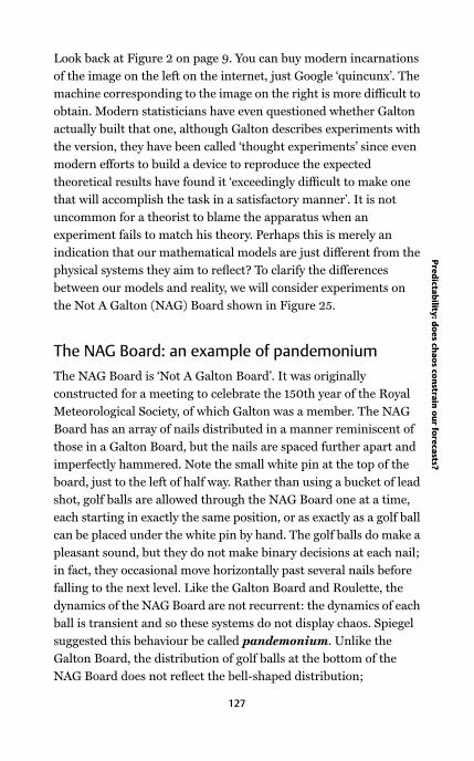
Look back at Figure 2 on page 9. You can buy modern incarnations

of the image on the left on the internet, just Google ‘quincunx’. The

machine corresponding to the image on the right is more difficult to

obtain. Modern statisticians have even questioned whether Galton

actually built that one, although Galton describes experiments with

the version, they have been called ‘thought experiments’ since even

modern efforts to build a device to reproduce the expected

theoretical results have found it ‘exceedingly difficult to make one

that will accomplish the task in a satisfactory manner’. It is not

uncommon for a theorist to blame the apparatus when an

experiment fails to match his theory. Perhaps this is merely an

indication that our mathematical models are just different from the

physical systems they aim to reflect? To clarify the differences

between our models and reality, we will consider experiments on

the Not A Galton (NAG) Board shown in Figure 25.

The NAG Board: an example of pandemonium

The NAG Board is ‘Not A Galton Board’. It was originally

constructed for a meeting to celebrate the 150th year of the Royal

Meteorological Society, of which Galton was a member. The NAG

Board has an array of nails distributed in a manner reminiscent of

those in a Galton Board, but the nails are spaced further apart and

imperfectly hammered. Note the small white pin at the top of the

board, just to the left of half way. Rather than using a bucket of lead

shot, golf balls are allowed through the NAG Board one at a time,

each starting in exactly the same position, or as exactly as a golf ball

can be placed under the white pin by hand. The golf balls do make a

pleasant sound, but they do not make binary decisions at each nail;

in fact, they occasional move horizontally past several nails before

falling to the next level. Like the Galton Board and Roulette, the

dynamics of the NAG Board are not recurrent: the dynamics of each

ball is transient and so these systems do not display chaos. Spiegel

suggested this behaviour be called pandemonium. Unlike the

Galton Board, the distribution of golf balls at the bottom of the

NAG Board does not reflect the bell-shaped distribution;

127

Pre

dicta

bility

: do

es ch

ao

s con

strain

ou

r fore

casts?

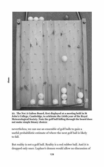
nevertheless, we can use an ensemble of golf balls to gain a

useful probabilistic estimate of where the next golf ball is likely

to fall.

But reality is not a golf ball. Reality is a red rubber ball. And it is

dropped only once. Laplace’s demon would allow no discussion of

25. The Not A Galton Board, first displayed at a meeting held in StJohn’s College, Cambridge, to celebrate the 150th year of the RoyalMeteorological Society. Note the golf ball falling through the board doesnot make simple binary choices

128

Ch

ao

s

what else might have happened: nothing else could have happened.

The analogy here is to take the red rubber ball as the Earth’s

atmosphere and the golf balls as our model ensemble members. We

can invest in as many members as we choose. But what does our

distribution of golf balls tell us about the single passage of the red

rubber ball? Surely the diversity of behaviour we observe between

golf balls tells us something useful? If nothing else, it give us a lower

bound on our uncertainty beyond which we know we cannot be

confident; but it can never provide a bound in which we can be

absolutely confident, even in probabilistic terms. By close analogy,

examining the diversity of our models can be very useful, even if

there is no probability forecast in sight.

The red ball is much like a golf ball: it has a diameter slightly larger

but roughly the same as a golf ball and it has, somewhat more

roughly, a similar elasticity. But the red ball which is reality can do

things that a golf ball simply cannot do: some unexpected, some

not; some relevant to our forecast, some not; some known, some

not. In the NAG Board, the golf ball is a good model of reality, a

useful model of reality; and an imperfect model of reality. How are

we to interpret this distribution of golf balls? No one knows.

Welcome to frontline statistical research. And it gets better. We

could always interpret the distribution of golf balls as a probability

forecast conditioned on the assumption that reality is a golf ball.

Would it not be a double-sense to proffer probability forecasts one

knew were conditioned on an imperfect model as if they reflected

the likelihood of future events, regardless of what small print

appeared under the forecast?

Our ensembles are not restricted to using only golf balls. We might

obtain green rubber balls of a slightly smaller diameter and repeat

the experiment. If we get a distribution of green balls similar to our

distribution of golf balls, we might take courage – or better, take

hope – that the inadequacies of our model might not play such a

large role in the forecast we are interested in. Alternatively, our two

models may share some systematic deficiency of which we are not

129

Pre

dicta

bility

: do

es ch

ao

s con

strain

ou

r fore

casts?

aware . . . yet. But what if the distributions of golf balls and green

balls are significantly different? Then we cannot sensibly rely on

either. How might quantifying the diversity of our models with

these multi-model ensembles allow us to construct a probabilistic

forecast for the one passage of reality? When we look at seasonal

weather forecasts, using the best models in the world, the

distribution from each model tends to cluster together, each in a

different way. How are we to provide decision support in this case,

or a forecast? What should be our aim? Indeed, how exactly can we

take aim at any goal given only empirically inadequate models? If

we naıvely interpret the diversity of an ensemble of models as a

probability, we will be repeatedly misled; we know at the start that

our models are imperfect, so any discussion of ‘subjective

probability’ is a red herring: we do not believe in (any of) our

models in the first place!

The bottom line is rather obvious: if our models were perfect and

we had the resources of Laplace’s demon, we would know the

future; while if our models were perfect and we had the resources of

our 21st-century demon, then chaos would restrict us to probability

forecasts, even if we knew the Laws of Nature were deterministic. In

case the True Laws of Nature are stochastic, we can envision a

statistician’s demon, which will again offer accountable probability

forecasts with or without exact knowledge of the current state of the

universe. But is the belief in the existence of mathematically precise

Laws of Nature, whether deterministic or stochastic, any less

wishful thinking than the hope that we will come across any of our

various demons offering forecasts in the woods?

In any event, it seems we do not currently know the relevant

equations for simple physical systems, or for complicated ones. The

study of chaos suggests that difficulty lies not with uncertainty in

the number to ‘put in’ but the lack of an empirically adequate model

to put anything into: chaos we might cope with, but it is model

inadequacy, not chaos, that limits predictability. A model may

undeniably be the best in the world, but that says nothing about

130

Ch

ao

s

whether or not it is empirically relevant, much less useful in

practice, or even safe. Forecasters who couch predictions they

expect to be fundamentally flawed with sleight-of-hand phrases

such as ‘assume the model is perfect’ or ‘best available information’,

may be technically speaking the truth, but if those models cannot

shadow the past then it is not clear what ‘uncertainty in the initial

state’ might mean. Those who blame chaos for the shortcomings of

probability forecasts they devised under the assumption their

models were perfect, models they knew to be inadequate, palter to

us in a double-sense.

131

Pre

dicta

bility

: do

es ch

ao

s con

strain

ou

r fore

casts?

Chapter 10

Applied chaos: can we see

through our models?

All theorems are true,

All models are wrong.

All data are inaccurate.

What are we to do?

Scientists often underestimate the debt they owe real-time

forecasters who, day after day, stand up and present their vision of

the future. Prominent among them are weather forecasters and

economists, while professional gamblers risk more than their image

when they go to work. As do futures traders. The study of chaos has

initiated a rethink of modelling and clarified the restrictions on

what we can see through our models. The implications differ, of

course, for mathematical systems where we know there is a target to

take aim at, and physical systems where what we aim for may well

not exist.

Modelling from the ground up: data-based models

We will consider four types of data-based models. The simplest are

persistence models which assume that things will stay as they are

now. A simple dynamic variation on this theme are advection

models, which assume the persistence of velocities: here, a storm

moving to the east would be forecast to continue moving to the east

at the same speed. Fitzroy and LeVerrier employed this approach in

132

the 1800s, exploiting telegraph signals which could race ahead of an

oncoming storm. The third are analogue models. Lorenz’s classic

1963 paper ends with the sentence: ‘In the case of the real

atmosphere, if all other methods fail, we can wait for an analogue.’

An analogue model requires a library of past observations from

which a previous state similar to the current state is identified; the

known evolution of this historical analogue provides the forecast.

The quality of this method depends on how well we observe the

state and whether or not our library contains sufficiently good

analogues. When forecasting a recurrent system, obtaining a good

analogue is just a question of whether or not the library’s collection

is large enough given our aims and the noise level. In practice,

building the library may require more than just patience: how

might we proceed if the expected time required to observe

recurrence is longer than the lifetime of the system itself?

Traditional statistics has long exploited these three approaches

within the context of forecasting from historical statistics. Takens’

Theorem suggests that for chaotic systems we can do better than

any of them. Suppose we wish to forecast what the state of the

atmosphere will be tomorrow from a library. The situation is shown

schematically in Figure 26. The analogue approach is to take the

state in the library which is nearest to today’s atmospheric state,

and report whatever it did the next day as our forecast for

tomorrow. Takens’ Theorem suggests taking a collection of nearby

analogues and interpolating between their outcomes to form our

forecasts. These data-based delay reconstruction models can prove

useful without being perfect: they need only outperform – or merely

complement – the other options available to us. Analogue

approaches remain popular in seasonal weather forecasting, while

roulette suggests a data-based modelling success story.

It is easy to put money on a winner in roulette: all you have to do is

bet one dollar on each number and you’ll have a winner every time.

You’ll lose money, of course, since your winner will pay $36, while

you’ll have to bet on more than 36 numbers. ‘Play them all’

133

Ap

plie

d ch

ao

s: can

we

see

thro

ug

h o

ur m

od

els?

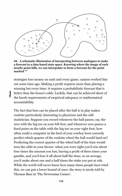
strategies lose money on each and every game; casinos worked this

out some time ago. Making a profit requires more than placing a

winning bet every time: it requires a probabilistic forecast that is

better than the house’s odds. Luckily, that can be achieved short of

the harsh requirements of empirical adequacy or mathematical

accountability.

The fact that bets can be placed after the ball is in play makes

roulette particularly interesting to physicists and the odd

statistician. Suppose you record whenever the ball passes, say, the

zero with the big toe on your left foot, and whenever zero passes a

fixed point on the table with the big toe on your right foot; how

often could a computer in the heel of your cowboy boot correctly

predict which quarter of the roulette wheel the ball would land on?

Predicting the correct quarter of the wheel half of the time would

turn the odds in your favour: when you were right you’d win about

four times the amount you lost, leaving a profit of three times your

gamble, and you’d lose it all about half the time; so on average,

you’d make about one and a half times the stake you put at risk.

While the world will never know how many times people have tried

this, we can put a lower bound of once: the story is nicely told by

Thomas Bass in ‘The Newtonian Casino’.

26. A schematic illustration of interpreting between analogues to makea forecast in a data-based state space. Knowing where the image of eachnearby point falls, we can interpolate to form a forecast for the pointmarked ‘*’

134

Ch

ao

s

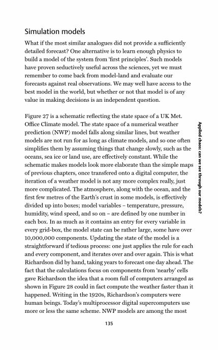
Simulation models

What if the most similar analogues did not provide a sufficiently

detailed forecast? One alternative is to learn enough physics to

build a model of the system from ‘first principles’. Such models

have proven seductively useful across the sciences, yet we must

remember to come back from model-land and evaluate our

forecasts against real observations. We may well have access to the

best model in the world, but whether or not that model is of any

value in making decisions is an independent question.

Figure 27 is a schematic reflecting the state space of a UK Met.

Office Climate model. The state space of a numerical weather

prediction (NWP) model falls along similar lines, but weather

models are not run for as long as climate models, and so one often

simplifies them by assuming things that change slowly, such as the

oceans, sea ice or land use, are effectively constant. While the

schematic makes models look more elaborate than the simple maps

of previous chapters, once transfered onto a digital computer, the

iteration of a weather model is not any more complex really, just

more complicated. The atmosphere, along with the ocean, and the

first few metres of the Earth’s crust in some models, is effectively

divided up into boxes; model variables – temperature, pressure,

humidity, wind speed, and so on – are defined by one number in

each box. In as much as it contains an entry for every variable in

every grid-box, the model state can be rather large, some have over

10,000,000 components. Updating the state of the model is a

straightforward if tedious process: one just applies the rule for each

and every component, and iterates over and over again. This is what

Richardson did by hand, taking years to forecast one day ahead. The

fact that the calculations focus on components from ‘nearby’ cells

gave Richardson the idea that a room full of computers arranged as

shown in Figure 28 could in fact compute the weather faster than it

happened. Writing in the 1920s, Richardson’s computers were

human beings. Today’s multiprocessor digital supercomputers use

more or less the same scheme. NWP models are among the most

135

Ap

plie

d ch

ao

s: can

we

see

thro

ug

h o

ur m

od

els?

complicated computer codes ever written and often produce

remarkably realistic-looking simulations. Like all models, however,

they are imperfect representations of the real-world system they

target, and the observations we use to initialize them are noisy. How

are we to use such valuable simulations in managing our affairs?

Can we at least get an idea of how much we should rely on today’s

forecast for next weekend?

27. A schematic reflecting the way weather and climate models divideboth the atmosphere and the ocean into ‘‘grid points’’. Here each gridpoint in the atmosphere represents approximately a 250 km by 250 kmsquare, which means that about six points account for the whole ofBritain as shown above

136

Ch

ao

s

28. A realization of Richardson’s dream,in which human computers work inmassively parallel style to calculate theweather before it happens. Note thedirector in the central platform is shininga light on northern Florida, presumablyindicating that those computers areslowing down the project (or perhaps theweather there is just particularly tricky tocompute?)

Ensemble weather prediction systems

Latest EPS giving northern France an edge over Cornwall. Do you

have a travel agent who can advise on ferry bookings? Tim

email dated 5 August 1999

In 1992 operational weather forecasting centres on both sides of the

Atlantic took a great step forward: they stopped trying to say exactly

what the weather would be next weekend. For decades, they had

run their computer simulations once a day. As computers grew

faster, the models had grown more and more complicated, limited

only by the need to get the forecast out well before the weather

arrived. This ‘best guess’ mode of operation ended in 1992: instead

of running the most complicated computer simulation once and

then watching as reality did something different, a slightly less

complex model was run a few dozen times. Each member of this

ensemble was initialized at a slightly different state. The forecasters

then watched the ensemble of simulations spread out from each

other as they evolved in time towards next weekend, and used this

information to quantify the reliability of the forecast for each day.

This is an Ensemble Prediction System (EPS).

By making an ensemble forecast we can examine alternatives

consistent with our current knowledge of the atmosphere and our

models. This provides significant advantages for informed decision

support. In 1928, Sir Arthur Eddington predicted a solar eclipse

‘visible over Cornwall’ for 11 August 1999. I wanted to see this

eclipse. So did Tim Palmer, Head of the Probability Forecast

Division at the European Centre for Medium-range Weather

Forecasts (ECMWF) in Reading, England. As the eclipse

approached, it seemed Cornwall might be overcast. The email from

Tim quoted at the beginning of this section was sent six days

before the eclipse: we examined the ensemble for the 11th, noting

that the number of ensemble members suggested clear sky over

France exceeded the corresponding number for Cornwall; the same

thing happened on the 9th and we left England for France by ferry.

138

Ch

ao

s

There we saw the eclipse, thanks to playing the odds suggested by

the EPS, and to a last minute dash for better visibility made

possible by Tim’s driving skills on tiny French farm roads in a

right-hand-drive car; not to mention his solar eclipse black-out

glasses. The study of chaos in our model suggests that our

uncertainty in the current state of the atmosphere makes it

impossible to say for certain, even only a week in advance, where

the eclipse will be visible and where it will be obscured by clouds.

By running an ensemble forecast with the aim of tracking this

uncertainty, the EPS provided effective decision support

nevertheless: we saw the eclipse. We did not have to assume

anything about the perfection of the model and there were no

probability distributions in sight.

Since the EPS first became operational in 1992, no ensemble

forecast was generated for the Burns’ Day storm of January 1990.

ECMWF has kindly generated a retrospective ensemble forecast

using the data available two days before the Burns’ Day storm

struck. Figure 4 (on page 14) shows the storm as seen within a

modern weather model – called the analysis – along with a

two-day-ahead forecast using only data from before the time of

the critical ship observations discussed in Chapter 1. Note that

there is no storm in the forecast. Twelve other ensemble members

also from two days before the storm are shown in Figure 29;

some have storms, some not. The second ensemble member in

the top row looks remarkably like the analysis; the member two

rows below it has what looks like a super-storm while other

members suggest a normal British winter’s day. As the critical

ship observations were made after this EPS forecast, this

ensemble would have already provided an indication that a

storm was likely, and significantly reduced the pressure on the

intervention forecaster. At longer lead times, the ensemble from

three days before Burns’ Day has members with storms over

Scotland, and there is even one member from the four-day-ahead

ensemble forecast with a major storm in the vicinity. The ensemble

provides early warning.

139

Ap

plie

d ch

ao

s: can

we

see

thro

ug

h o

ur m

od

els?

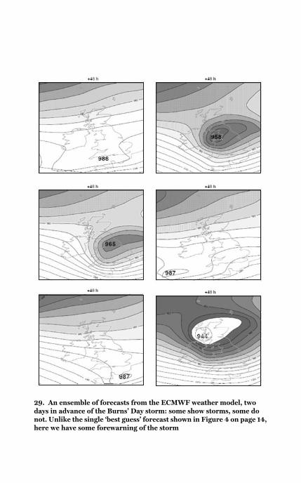
29. An ensemble of forecasts from the ECMWF weather model, twodays in advance of the Burns’ Day storm: some show storms, some donot. Unlike the single ‘best guess’ forecast shown in Figure 4 on page 14,here we have some forewarning of the storm

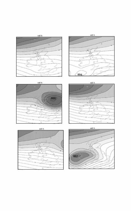
At all lead times, we must cope with the Burns effect: our collection

of ECMWF weather ‘golf balls’ shows the diversity of our model’s

behaviour to aid us when we ‘guess and fear’, without actually

quantifying the uncertainty in our real-world future. In fact, we

could widen this diversity, if we have enough computer power and

questioned the reliability of certain observations, we might run

some ensemble members with those observations while omitting

them in others. We will never see another situation quite like the

Burns’ Day storm of 1990. We might decide where to take future

observations designed to maximize the chance of distinguishing

which of our ensemble members were most realistic: those with a

storm in the future or those without?

Rather than wasting too much energy trying to determine the ‘best’

model, we might learn that ensembles members from different

models were of more value than one simulation of an extremely

expensive super-model. But we should not forget the lessons of the

NAG Board: our ensembles reveal the diversity of our models not

the probability of future events. We can examine ensembles over

initial conditions, parameter values, even mathematical model

structures, but it seems only our 21st-century demon can make

probability forecasts which are useful as such. Luckily, an EPS can

inform and add value without providing probabilities that we would

use as such for decision making.

Just after Christmas in 1999, another major storm swept across

Europe. Called T1 in France and Lothar in Germany, this storm

destroyed 3,000 trees in Versailles alone and set new record high

insurance claims in Europe. Forty-two hours before the storm,

ECMWF ran its usual 51-member EPS forecast. Fourteen members

of the 51-member ensemble had storms. It is tempting to forget

these are but as golf balls on a NAG Board, and interpret this as

saying that there was about a 28% probability of a major storm.

Even though that temptation should be resisted, we have here

another EPS forecast with great utility. Running a more realistic,

more complicated model once might have shown a storm, or might

142

Ch

ao

s

have shown no storm: why take the chance of not seeing the storm

when an EPS might quantify that chance? Ensemble forecasting is

clearly a sensible idea, but how exactly should we distribute limited

resources between using a more expensive model and making a

larger ensemble? This active research question remains open. In the

meantime, the ECMWF EPS regularly provides a glimpse of

alternative future scenarios seen through our models with

significant added value.

How to communicate this information in the ensemble without

showing the public dozens of weather maps also remains an open

question. In New Zealand, where severe weather is rather common,

the Meteorological Service regularly makes useful probabilistic

statements on their website – statements like ‘two chances in five’.

This adds significant value to the description of a likely event. Of

course, meteorologists often display a severe weather fetish, while

energy companies are happy to exploit the significant economic

value in extracting useful information from more mundane

weather, every day. And those in other sectors with operational

weather risk are beginning to follow suit.

Chaos and climate change

Climate is what you expect. Weather is what you get.

Robert Heinlein, Time Enough for Love (1974)

Climate modelling differs fundamentally from weather

forecasting. Think of the weather in the first week in January a

year from now. It will be mid-summer in Australia and mid-

winter in the northern hemisphere. That alone gives us a good

idea of the range of temperatures to expect: this collection of

expectations is climate – ideally reflecting the relative probability

of every conceivable weather pattern. If we believe in physical

determinism, then the weather next January is already

preordained; even so, our concept of the climate collection is

relevant, as our current models are not able to distinguish that

143

Ap

plie

d ch

ao

s: can

we

see

thro

ug

h o

ur m

od

els?

preordained future. The ideal ensemble weather forecast would

trace the growth of any initial uncertainty in the state of the

atmosphere until it became indistinguishable from the

corresponding climate distribution. Given imperfect models, of

course, this doesn’t ever quite happen, as our ensemble of model

simulations evolves towards the attractor of the model not that of

the real world, if such a thing exists. Even with a perfect model,

and ignoring the impacts of human free will noted by Eddington,

accurate probability forecasts based on the current conditions of

the Earth would be prevented by influences just now leaving the

Sun, or those due to arrive from beyond the solar system, of

which we cannot know today, even in principle.

Climate modelling also differs from weather forecasting in that it

often contains a ‘what if’ component. Altering the amount of carbon

dioxide (CO2) and other greenhouse gases in the atmosphere is

analogous to changing the parameter α in the Logistic Map; as we

change parameter values, the attractor itself changes. In other

words, while weather forecasters try to interpret the implications a

distribution of golf balls holds for the single drop of a red rubber

ball in the NAG Board of Figure 25 (page 128), climate modellers

add the complication of asking what would happen if the nails were

moved about.

Looking at just one run of a climate model carries the same dangers

as looking at just one forecast for Burns’ Day in 1990, although the

repercussions of such naıve over-confidence would be much greater

in the climate case. No computing centre in the world has the power

to run large ensembles of climate models. Nevertheless, such

experiments are made possible by harnessing the background

processing power of PCs in homes spread about the globe (see

www.climateprediction.net). Thousands of simulations have

revealed that a surprisingly large range of diversity exists within one

state-of-the-art climate model, suggesting that our uncertainty in

the future of real-world climate is at least very large. These results

contribute to improving current models. They fail to provide

144

Ch

ao

s

evidence that the current generation of climate models can

realistically focus the questions of regional detail, which, when

available, will be of great value in decision support. A frank

appraisal of the limitations of today’s climate models casts little

doubt upon the wide consensus that significant warming has been

seen in the data of the recent past.

How wide is the current diversity among our models? This depends,

of course, on what model variables you examine. In terms of planet-

wide average temperature, there is a consistent picture of warming;

a goodly number of ensemble members show a great deal more

warming than was previously considered. In terms of regional

details, there are vast variations between ensemble members. It is

hard to judge the utility of estimated precipitation for decision

support, even for monthly rainfall over the whole of Europe. How

might one distinguish what are merely the best currently available

forecasts from forecasts that actually contain useful information for

decision makers in the climate context?

In reality, carbon dioxide levels and other factors are constantly

changing, weather and climate merge into a single realization of a

one-off transient experiment. Weather forecasters often see

themselves as trying to extract useful information from the

ensemble before it spreads out across the ‘weather attractor’;

climate modellers must address difficult questions about how the

structure of that attractor would change if, say, the amount

of carbon dioxide in the atmosphere was doubled and then held

constant. Lorenz was already doing active research here in the

1960s, warning that issues of structural stability and long transients

complicate climate forecasts, and illustrating the effects in systems

not much more complicated than the maps we defined in Chapter 3.

Given that our weather models are imperfect, their ensembles do

not actually evolve towards realistic climate distributions. And

given that the properties of the Earth’s climate system are

constantly changing, it makes little sense to talk about some

145

Ap

plie

d ch

ao

s: can

we

see

thro

ug

h o

ur m

od

els?

constantly changing, unobservable ‘realistic climate distribution’ in

the first place. Could any such thing exist outside of model-land?

That said, coming to understand chaos and nonlinear dynamics has

improved both the experimental design in and the practice of

climate studies, allowing more insightful decision support for

policy makers. Perhaps most importantly, it has clarified that

difficult decisions will have to be made under uncertainty. Neither

the fact that this uncertainty is not tightly constrained nor the fact

that it can only be quantified with imperfect models, provides an

excuse for inaction. All difficult policy decisions are made in the

context of the Burns effect.

Chaos in commerce: new opportunities in Phynance

When a large number of people are playing a game with clear rules

but unknown dynamics, it is hard to distinguish those who win with

skill from those who win by chance. This is a fundamental problem

in judging hedge-fund managers and improving weather models,

since traditional scores can actually penalize skilful probabilistic

play. The Prediction Company, or PredCo, was founded on the

premise that there must be a better way to predict the economic

markets than the linear statistical methods that dominated

quantitative finance two decades ago. PredCo set out upon a

different path blazed by Doyne Farmer and Norm Packard, along

with some of the brightest young nonlinear dynamicists of the day,

who gave up post-docs for stock options. If there was chaos in the

markets, perhaps others were being be fooled without randomness?

Sadly, confidentiality agreements still cloud even PredCo’s early

days, but the continued profitability of the company indicates that

whatever it is doing, it is doing it well.

PredCo is one example of a general move towards Phynance,

bringing well-trained mathematical physicists in to look at forecast

problems in finance, traditionally the statistician’s preserve. Is the

stock market chaotic? Current evidence suggests our best models of

the markets are fundamentally stochastic, so the answer is ‘no’. But

146

Ch

ao

s

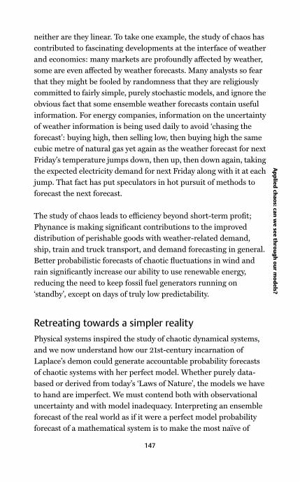
neither are they linear. To take one example, the study of chaos has

contributed to fascinating developments at the interface of weather

and economics: many markets are profoundly affected by weather,

some are even affected by weather forecasts. Many analysts so fear

that they might be fooled by randomness that they are religiously

committed to fairly simple, purely stochastic models, and ignore the

obvious fact that some ensemble weather forecasts contain useful

information. For energy companies, information on the uncertainty

of weather information is being used daily to avoid ‘chasing the

forecast’: buying high, then selling low, then buying high the same

cubic metre of natural gas yet again as the weather forecast for next

Friday’s temperature jumps down, then up, then down again, taking

the expected electricity demand for next Friday along with it at each

jump. That fact has put speculators in hot pursuit of methods to

forecast the next forecast.

The study of chaos leads to efficiency beyond short-term profit;

Phynance is making significant contributions to the improved

distribution of perishable goods with weather-related demand,

ship, train and truck transport, and demand forecasting in general.

Better probabilistic forecasts of chaotic fluctuations in wind and

rain significantly increase our ability to use renewable energy,

reducing the need to keep fossil fuel generators running on

‘standby’, except on days of truly low predictability.

Retreating towards a simpler reality

Physical systems inspired the study of chaotic dynamical systems,

and we now understand how our 21st-century incarnation of

Laplace’s demon could generate accountable probability forecasts

of chaotic systems with her perfect model. Whether purely data-

based or derived from today’s ‘Laws of Nature’, the models we have

to hand are imperfect. We must contend both with observational

uncertainty and with model inadequacy. Interpreting an ensemble

forecast of the real world as if it were a perfect model probability

forecast of a mathematical system is to make the most naıve of

147

Ap

plie

d ch

ao

s: can

we

see

thro

ug

h o

ur m

od

els?

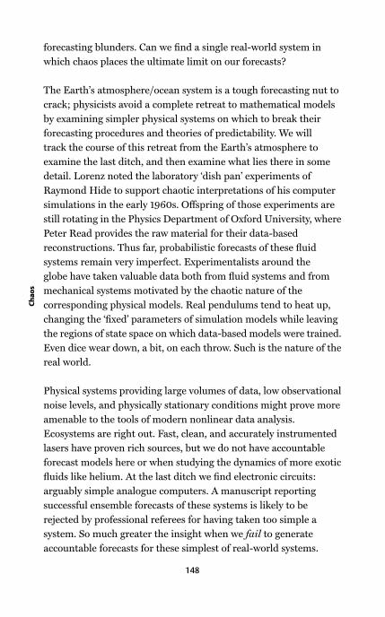
forecasting blunders. Can we find a single real-world system in

which chaos places the ultimate limit on our forecasts?

The Earth’s atmosphere/ocean system is a tough forecasting nut to

crack; physicists avoid a complete retreat to mathematical models

by examining simpler physical systems on which to break their

forecasting procedures and theories of predictability. We will

track the course of this retreat from the Earth’s atmosphere to

examine the last ditch, and then examine what lies there in some

detail. Lorenz noted the laboratory ‘dish pan’ experiments of

Raymond Hide to support chaotic interpretations of his computer

simulations in the early 1960s. Offspring of those experiments are

still rotating in the Physics Department of Oxford University, where

Peter Read provides the raw material for their data-based

reconstructions. Thus far, probabilistic forecasts of these fluid

systems remain very imperfect. Experimentalists around the

globe have taken valuable data both from fluid systems and from

mechanical systems motivated by the chaotic nature of the

corresponding physical models. Real pendulums tend to heat up,

changing the ‘fixed’ parameters of simulation models while leaving

the regions of state space on which data-based models were trained.

Even dice wear down, a bit, on each throw. Such is the nature of the

real world.

Physical systems providing large volumes of data, low observational

noise levels, and physically stationary conditions might prove more

amenable to the tools of modern nonlinear data analysis.

Ecosystems are right out. Fast, clean, and accurately instrumented

lasers have proven rich sources, but we do not have accountable

forecast models here or when studying the dynamics of more exotic

fluids like helium. At the last ditch we find electronic circuits:

arguably simple analogue computers. A manuscript reporting

successful ensemble forecasts of these systems is likely to be

rejected by professional referees for having taken too simple a

system. So much greater the insight when we fail to generate

accountable forecasts for these simplest of real-world systems.

148

Ch

ao

s

Figure 30 shows ensemble forecasts of observed voltages in a circuit

constructed to mimic the Moore-Spiegel system. Forecasts from

two different models are shown. In each panel, the dark solid line

shows the target observations generated by the circuit, while each

light line is an ensemble member; the forecasts start at time equals

zero; the ensemble was formed using only observations taken

before that time. The top two panels show results from Model One,

while the bottom two show results from Model Two. Look at the two

panels on the left, which show simultaneous forecasts from each

model. Every member of the Model One ensemble runs away from

reality without warning just before time 100, as shown in the upper

panel; the Model Two ensemble in the lower panel manages to

spread out at about the correct time (or is it a bit early?), and the

diversity of this ensemble looks useful all the way to the end of the

forecast. In this case, we may not know which model was going to

prove correct, but we can see where they began to strongly diverge

from each other. On the panels to the right, both models fail at

about the same time, in about the same way.

In each case, it appears that the forecasts provide insight into the

likely future observations, but that the point in the future when this

insight fails is not well reflected by either ensemble system. How

can we best interpret this diversity in terms of a forecast?

Analysis of many forecasts from different initial conditions shows

that, interpreted as probability forecasts, these ensembles are not

accountable. This seems to be a general result when using arguably

chaotic mathematical models to forecast real-world systems. I know

of no exceptions. Luckily, utility does not require extracting useful

probability estimates.

Odds: do we really have to take our modelsso seriously?

In academic mathematics, odds and probabilities are more or less

identical. In the real world this is not the case. If we add up the

149

Ap

plie

d ch

ao

s: can

we

see

thro

ug

h o

ur m

od

els?

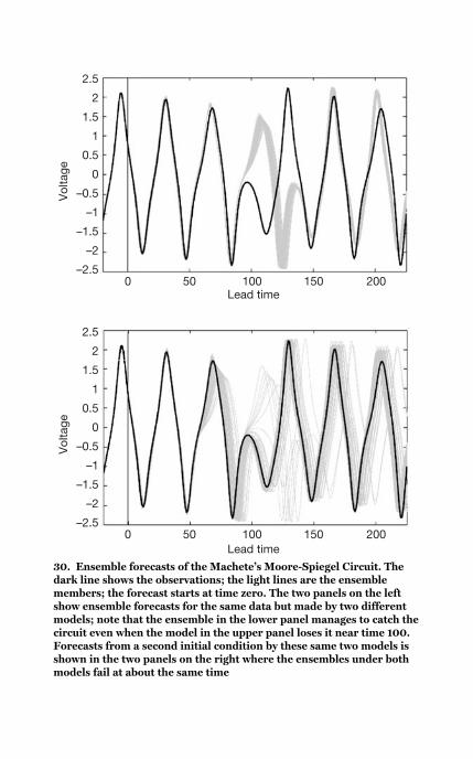
30. Ensemble forecasts of the Machete’s Moore-Spiegel Circuit. Thedark line shows the observations; the light lines are the ensemblemembers; the forecast starts at time zero. The two panels on the leftshow ensemble forecasts for the same data but made by two differentmodels; note that the ensemble in the lower panel manages to catch thecircuit even when the model in the upper panel loses it near time 100.Forecasts from a second initial condition by these same two models isshown in the two panels on the right where the ensembles under bothmodels fail at about the same time

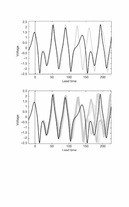
probability of every possible event, then the sum of the probabilities

should be one. For any particular set of odds-on, we can then define

the implied probability of an event from the odds on that event. If

the sum of the implied probabilities is equal to one, then this set of

odds are probabilistic odds. Outside mathematics lectures,

probabilistic odds are rather hard to find in the real world. The

related notion of ‘fair odds’, where the odds are fixed and one is

given the option to take either side of a bet, suggests a similar sort of

ivory tower ‘wishful thinking’; implied probabilities from odds-

against do not complement those from odds-on. The confusion at

the heart of both conceptions comes largely from blurring the

distinction between mathematical systems and the real-world

systems they model. At the racetrack or in a casino, the implied

probabilities sum to more than one. A European roulette wheel

yields 37/36, while an American wheel yields 38/36. In a casino this

excess ensures profit; scientifically, we might exploit this same

excess to communicate information about model inadequacy.

Model inadequacy can steer us away from probability forecasts in a

manner not dissimilar to the way in which uncertainty in the initial

condition steers us away from the principle of least squares in

nonlinear models. Theory for incorporating probability forecast

systems into a decision support by maximizing expected utility – or

some other reflection of the user’s goal – is well developed. A

‘probability forecast’ which would not be used as such in this setting

should perhaps not be called a probability forecast at all. A theory

for incorporating forecast systems which provides odds rather than

probabilities for decision support could, no doubt, be constructed.

Judd has already provided several worked examples.

It appears that accepting the inadequacy of our own models, while

being ignorant of the inadequacy of the models to which the

competition has access, requires we aim for something short of fair

odds. If an odds prediction system can cover its losses – breaking

even when evaluated over all comers while covering its running

costs – then we can say it generates sustainable odds. Sustainable

152

Ch

ao

s

odds then provide decision support which does not result (has not

yet resulted) in catastrophe nor instilled the desire to invest more in

improving those odds in order either to gain greater market share

or to cover running expenses.

Ensembles over all the alternatives one can think of to sample

might lead to sustainable odds, allowing the diversity within

multi-model ensembles to estimate the impact of model

inadequacy. The extent to which the sum of our implied

probabilities exceeds one provides a manner to quantify model

inadequacy. One wonders if, as we understand some real-world

system better and better, we can expect the implied probabilities of

our odds forecasts to ever sum to one for any physical system?

Moving to forecast systems which provide odds rather than

probabilities releases our real-world decision support from

unnatural constraints due to probabilities, which may be well-

defined only in our mathematical systems. It is an awkward but

inescapable fact that sustainable odds will depend both on the

quality of your model and on that of the opposition. Decision

making would be easy if accountable probability forecasts were on

offer, but when model diversity cannot be translated into (a decision

relevant) probability, we have no access to probability forecasts.

Pursuing risk management as if we did for the sake of simplicity is

foolhardy. And while odds might prove useful in hourly or daily

decision making, what are we to do in the climate change scenario,

where it appears we have only one high-impact event and no truly

similar test cases to learn from?

We have reached the coal face of real-world scientific forecasting.

The old seam of probability is growing thin and it is unclear exactly

which direction we should dig in next. If chaotic dynamical systems

have not provided us with a new shovel, they have at least given us a

canary.

153

Ap

plie

d ch

ao

s: can

we

see

thro

ug

h o

ur m

od

els?

Chapter 11

Philosophy in chaos

You don’t have to believe everything you compute.

Is there really anything new in chaos? There is an old joke about

three baseball umpires discussing the facts of life within the game.

The first umpire says ‘I calls’em as I see’em.’ The second umpire says

‘I calls’em as they are.’ Finally, the third says ‘They ain’t, until I

calls’em.’ The study of chaos tends to force us towards the

philosophical position of the third referee.

Complications of chaos

Do the quantities we forecast exist only within the forecast models

we construct? If so, then how might we contrast them with our

observations? A forecast lies in the state space of our model and,

while the corresponding observation is not in that state space,

are these two ‘subtractable’? This is a mathematical version of

the ‘apples and oranges’ problem: are the model state and

the observation similar enough that we can meaningfully

subtract one from the other to define a distance, to then call a

forecast error? Or are they not? And if not, then how might we

proceed?

Evaluation of chaotic models has exposed a second fundamental

complication that arises even in perfect nonlinear models with

154

unknown parameter values: how do we determine the best

values? If the model is linear, then we have several centuries

of experience and theory which convincingly establish that the

best values in practice are those that yield the closest agreement

on the target data, where closest is defined in a least squares

sense (smallest distance between the model and the target

observations); likelihood is a useful thing to maximize. If our

model is not linear, then our centuries of intuition often prove a

distraction, if not an impediment to progress. Taking least squares

is no longer optimal, and the very idea of ‘accuracy’ has to be

rethought. This simple fact is as important as it is neglected.

This problem is easily illustrated in the Logistic Map: given the

correct mathematical formula and all the details of the noise

model – random numbers with a bell-shaped distribution –

using least squares to estimate α leads to systematic errors.

This is not a question of too few data or insufficient computer

power, it is the method that fails. We can compute the optimal

least squares solution: its value for α is too small at all noise

levels. This principled approach just does not apply to nonlinear

models because the theorems behind the principle of least

squares repeatedly assume bell-shaped distributions. The shape

of these distributions is preserved by linear models, but

nonlinear models distort the bell-shape, making least squares

inappropriate. In practice, this ‘wishful linear thinking’

systematically underestimates the true parameter value at

every noise level. Recent (mis)interpretations of climate

models have floundered due to similarly wishful linear thinking.

Our 21st-century demon will be able to estimate α very accurately,

but she will not be using least squares to do so! (She will be looking

for shadows.)

Philosophers have also wondered whether fractal intricacy might

establish the existence of real numbers in nature, proving that

irrational numbers exist even if we can only see a few of the

leading bits. Strange attractors offer nothing to support such

arguments that cannot be obtained from linear dynamical

155

Ph

iloso

ph

y in

cha

os

systems. On the other hand, chaos offers a new way to use both

models and our observations to define variables in remarkable

detail – if our models are good enough – via states along the shadow

from an empirically adequate nonlinear model. If our model

shadows the observations for an extended time, then all the

shadowing states will fall into a very narrow range of values,

providing a way to define values for observables like temperature to

a precision beyond that at which our usual concept of temperature

breaks down. We will never get to an irrational number, but an

empirically adequate model could supply a definition of arbitrary

accuracy, using the observations while placing the model into a role

not unlike that of the third umpire. That said, the traditional

connection between temperature and our measurements of it via a

noise model, remains safe until useful shadowing trajectories are

shown to exist.

Another philosophical quandary arises in terms of how to define the

‘best’ forecast in practice. Probabilistic forecasts provide a

distribution as each forecast, while the target observation we verify

against will always be a single event: when the forecast distribution

differs from one forecast to the next, we have yet another ‘apples

and oranges’ problem and can never evaluate even one of our

forecast distributions as a distribution.

The success of our models tends to lull us towards the happy

thought that mathematical laws govern the real-world systems of

interest to us. Linear models formed a happy family. The wrong

linear model can be close to the right linear model, and seen to be

so, in a sense that does not apply to nonlinear models. It is not easy

to see that an imperfect nonlinear model is ‘close to’ the right model

given only observations: we can see that it allows long shadows, but

if the two models have different attractors – and we know that the

attractors of very similar mathematical models can be very different

– then we do not know how to make ensembles that produce

accountable probability forecasts. We must reconsider how our

nonlinear models might approach Truth, in the case that Truth can

156

Ch

ao

s

be encapsulated in some ‘right’ model. We have no scientific reason

to believe that such a perfect model exists. Our philosopher might

turn from muddy issues raised on the quest for Truth and

contemplate the implications of there being nothing more than

collections of imperfect models. What advice might she offer our

physicist? If new computer power allows the generation of

ensembles over everything we can think of (initial conditions,

parameter values, models, compilers, computer architecture, and so

on), how do we interpret the distributions that come out

scientifically? Or expose the folly of hiding from these issues behind

a single simulation from a particularly complicated ultra-high-

resolution model?

Lastly, note that when working with the wrong model, we may ask

the wrong question. Who is who in la Tour’s card game? The

question assumes a model in which each player can be only a

mathematician or a physicist or a statistician or a philosopher, and

that there must be a representative of each discipline at the table.

Perhaps this assumption is false. As real-world scientists, can each

of our players take on every role?

The burden of proof: what is chaotic, really?

If we stay with mathematical standards of proof, then very few

systems can be proven to be chaotic. The definition of mathematical

chaos can only be applied to mathematical systems, so we cannot

begin to prove a physical system is chaotic, or periodic for that

matter. Nevertheless, it is useful to describe physical systems as

periodic or chaotic as long as we do not confuse the mathematical

models with the systems we use them to describe. When we have

the model in hand, we can see whether it is deterministic or

stochastic, but even after knowing it to be deterministic, proving

it to be chaotic is non-trivial. Calculating Lyapunov exponents

is a difficult task, and there are very few systems for which we can

do this analytically. It took almost 40 years to establish a

mathematical proof that the dynamics of the 1963 Lorenz System

157

Ph

iloso

ph

y in

cha

os

were chaotic, so the question regarding more complicated

equations like those used for the weather is likely to remain open for

quite some time.

We cannot hope to defend a claim that a physical system is chaotic

unless we discard the mathematicians’ burden of proof, and with it

the most common meaning of chaos. Nevertheless, if our best

models of a physical system appear to be chaotic, if they are

deterministic, appear to be recurrent, and suggest sensitive

dependence by exhibiting the rapid growth of small uncertainties,

then these facts provide a working definition of what it means for a

physical system to be chaotic. We may one day find a better

description of that physical system which does not have these

properties, but that is the way of all science. In this sense, the

weather is chaotic while the economy is not. Does this imply that if

we were to add a so-called random number generator to our

weather model we no longer believe real weather is chaotic? Not at

all, as long as we only wish to employ a random number generator

for engineering reasons, like accounting for defects in the finite

computerized model. In a similar vein, the fact we cannot employ a

true random number generator in our computer models does not

imply we must consider the stock market deterministic. The study

of chaos has laid bare the importance of distinguishing between

our best models and the best way to construct computer

simulations of those models. If our model structure is imperfect,

our best models of a deterministic system might well turn out to be

stochastic!

Perhaps the most interesting question of all to come out of chaotic

forecasting is the open question of a fourth modelling paradigm: we

see our best model fail to shadow, we suspect that there is no way to

fix this model, either within the deterministic modelling scheme of

our physicist, or within the standard stochastic schemes of our

statistician. Can further study of mathematical chaos suggest a

synthesis that will give us access to models that can at least shadow

physical systems?

158

Ch

ao

s

Shadows, chaos, and the future

Our eyes once opened, we may pass on to a yet newer outlook of the

world, but we can never go back to the old outlook.

A. Eddington (1927)

Mathematics is the ultimate science fiction. While mathematicians

can happily limit their activities to domains where all their

assumptions hold (‘almost always’), physicists and statisticians

must deal with the external world through the data to hand and the

theories to mind. We must keep this difference in mind if we are

going to use words like ‘chaos’ when speaking with mathematicians

and scientists; a chaotic mathematical system is simply a different

beast than a physical system we call chaotic. Mathematics proves;

science struggles merely to describe. Failure to recognize this

distinction has injected needless acrimony into the discussion.

Neither side is ‘winning’ this argument, and as the previous

generation slowly leaves the field, it is interesting to observe some

members of the next generation adopt an ensemble approach:

neither selecting nor merging but literally adopting multiple

models as a model and using them in unison. Rather than playing

as adversaries in a contest, can our physicist, mathematician,

statistician, and philosopher work as a team?

The study of chaos helps us to see more clearly which questions

make sense and which are truly nonsensical: the study of chaotic

dynamics has forced us to accept that some of our goals are

unreachable given the awkward properties of nonlinear systems.

And given that our best models of the world are nonlinear – models

for the weather, the economy, epidemics, the brain, the Moore-

Spiegel circuit, even the Earth’s climate system – this insight has

implications beyond science, extending to decision support and

policy making. Ideally, the insights of chaos and nonlinear

dynamics will come to the aid of the climate modeller, who, when

asked to answer a question she knows to be meaningless, is

empowered to explain the current limits to our knowledge and

159

Ph

iloso

ph

y in

cha

os

communicate the available information. Even if model

imperfections imply that there is no policy-relevant probability

forecast, a better understanding of the underlying physical process

has aided decision makers for ages.

All difficult decisions are made under uncertainty; understanding

chaos has helped us to provide better decision support. Significant

economic progress has already been made in the energy sector,

where the profitability of using information-rich weather ensembles

has led to daily use of uncertainty information from trading floors of

the markets to the control rooms of national electricity grids.

Prophecy is difficult; it is never clear which context science will

adopt next, but the fact that chaos has changed the goal posts may

well be its most enduring impact on science. This message needs to

be introduced earlier in education; the role of uncertainty and the

rich variety of behaviour that mathematically simple systems reveal

is still largely unappreciated. Observational uncertainty is

inextricably melded with model error, forcing us to re-evaluate what

counts as a good model. Our old goal to minimize least squares has

been proven to mislead, but should we replace them with a search

for shadows, for a model with good-looking behaviour, or the ability

to make more accountable probability forecasts? From our new

vantage point, we can see more clearly which questions make sense,

calling forth challenges to the foundational assumptions of

mathematical physics and to applications of probability theory. Are

our modelling failures due to our inability to select the correct

answer from among the available options, or is there no suitable

option on offer? How do we interpret simulations from models

which are not empirically adequate? Regardless of our personal

beliefs on the existence of Truth, chaos has forced us to rethink what

it means to approximate Nature.

The study of chaos has provided new tools: delay reconstructions

that may yield consistent models even when we do not know the

‘underlying equations’, new statistics with which to describe

160

Ch

ao

s

dynamical systems quantitatively, new methods of forecasting

uncertainty, and shadows that bridge the gaps between our models,

our observations, and our noise. It has moved the focus from

correlation to information, from accuracy to accountability, from

artificially minimizing arguably irrelevant error to increasing utility.

It rekindles debate on the status of objective probability: can we

ever construct an operationally useful probability forecast, or are we

forced to develop novel ad hoc methods for using probabilistic

information without probability forecasts? Are we quantifying our

uncertainty in the future of the real world or exploring the diversity

in our models? Science seeks its own inadequacy; coping with

constant uncertainty in science is not a weakness but a strength.

Chaos has provided much new cloth for our study of the world,

without providing any perfect models or ultimate solutions. Science

is a patchwork, and some of the seams admit draughts.

Early in the film The Matrix, Morpheus echoes the words of

Eddington that open this last section:

This is your last chance. After this, there is no going back. You take

the blue pill and the story ends. You wake up in your bed and you

believe whatever you want to believe. You take the red pill and you

stay in Wonderland and I show you how deep the rabbit hole goes.

Remember that all I am offering is the truth. Nothing more.

Chaos is the red pill.

161

Ph

iloso

ph

y in

cha

os

This page intentionally left blank

Glossary

Mathematicians are like a certain type of Frenchman; when you talk

to them they translate it into their own language, and then it soon

turns into something completely different.

Goethe, Maxims and Reflections (1779)

These entries are not meant to provide precise definitions, but

are intended to convey the main idea for quick reference. Some

terms hold different shades of meaning when used by

mathematicians (M), physicists (P), computer scientists (C), or

statisticians (S). Definitions and discussion can be found in the

CATS’ Forum at www.lsecats.org and in books listed in the further

reading.

almost every (M): A mathematical catch phrase to warn that even

though something is 100% true, there are instances when it is false.

almost every (P): Almost every.

attractor: A point or collection of points in state space which some

other collection of states approach nearer and nearer as they are

iterated forward.

basin of attraction: For a particular attractor, the collection of all

states that will eventually approach it.

Burns effect: An expression that encapsulates the difficulty that

incomplete foresight and imperfect models bring to attempts at

rational decision making.

163

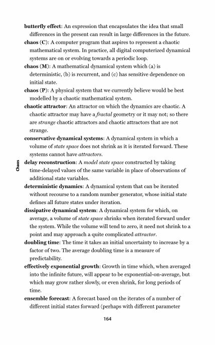
butterfly effect: An expression that encapsulates the idea that small

differences in the present can result in large differences in the future.

chaos (C): A computer program that aspires to represent a chaotic

mathematical system. In practice, all digital computerized dynamical

systems are on or evolving towards a periodic loop.

chaos (M): A mathematical dynamical system which (a) is

deterministic, (b) is recurrent, and (c) has sensitive dependence on

initial state.

chaos (P): A physical system that we currently believe would be best

modelled by a chaotic mathematical system.

chaotic attractor: An attractor on which the dynamics are chaotic. A

chaotic attractor may have a fractal geometry or it may not; so there

are strange chaotic attractors and chaotic attractors that are not

strange.

conservative dynamical systems: A dynamical system in which a

volume of state space does not shrink as it is iterated forward. These

systems cannot have attractors.

delay reconstruction: A model state space constructed by taking

time-delayed values of the same variable in place of observations of

additional state variables.

deterministic dynamics: A dynamical system that can be iterated

without recourse to a random number generator, whose initial state

defines all future states under iteration.

dissipative dynamical system: A dynamical system for which, on

average, a volume of state space shrinks when iterated forward under

the system. While the volume will tend to zero, it need not shrink to a

point and may approach a quite complicated attractor.

doubling time: The time it takes an initial uncertainty to increase by a

factor of two. The average doubling time is a measure of

predictability.

effectively exponential growth: Growth in time which, when averaged

into the infinite future, will appear to be exponential-on-average, but

which may grow rather slowly, or even shrink, for long periods of

time.

ensemble forecast: A forecast based on the iterates of a number of

different initial states forward (perhaps with different parameter

164

Ch

ao

s

values, or even different models) and in so doing reveals the diversity

of our model(s) and so provides a lower bound on the likely impacts of

uncertainty in model-based forecasts.

exponential growth: Growth where the rate of increase in X is

proportional to the value of X, so that as X gets larger, it grows even

faster.

fixed point: A state of a dynamical system which stays put; a

stationary point whose future value under the system is its current

value.

flow: A dynamical system in which time is continuous.

fractal: A self-similar collection of points or an object that is self-similar

in an interesting way (more interesting than, say, a smooth line or

plane). Usually, one requires a fractal set to have zero volume in the

space that it lives, as a line in two dimensions has no area, or a surface

in three dimensions has no volume.

geometric average: The result of multiplying N numbers together and

then taking the Nth root of the product.

indistinguishable state: One member of the collection of points which,

given an observational noise model, you would not expect to be able to

rule out as having generated the observations actually generated by

some target trajectory X. This collection is called the set of

indistinguishable states of X and has nothing to do with any

particular set of observations.

infinitesimal: A quantity smaller than any number you can name, but

strictly greater than zero.

iterate: To apply the rule defining a dynamical map once, moving the

state forward one step.

linear dynamical system: A dynamical system in which sums of

solutions are also solutions, more generally one that allows

superposition of solutions. (For technical reasons, we do not wish to

say ‘involves only linear rules’.)

Lyapunov exponent: A measure of the average speed with which

infinitesimally close states separate. It is called an exponent, since it

is the logarithm of the average rate, which makes it easy to distinguish

exponential-on-average growth (greater than zero) from exponential-

on-average shrinking (negative). Note that slower-than-exponential

165

Glo

ssary

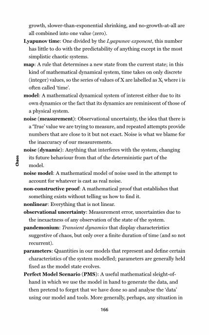
growth, slower-than-exponential shrinking, and no-growth-at-all are

all combined into one value (zero).

Lyapunov time: One divided by the Lyapunov exponent, this number

has little to do with the predictability of anything except in the most

simplistic chaotic systems.

map: A rule that determines a new state from the current state; in this

kind of mathematical dynamical system, time takes on only discrete

(integer) values, so the series of values of X are labelled as Xi where i is

often called ‘time’.

model: A mathematical dynamical system of interest either due to its

own dynamics or the fact that its dynamics are reminiscent of those of

a physical system.

noise (measurement): Observational uncertainty, the idea that there is

a ‘True’ value we are trying to measure, and repeated attempts provide

numbers that are close to it but not exact. Noise is what we blame for

the inaccuracy of our measurements.

noise (dynamic): Anything that interferes with the system, changing

its future behaviour from that of the deterministic part of the

model.

noise model: A mathematical model of noise used in the attempt to

account for whatever is cast as real noise.

non-constructive proof: A mathematical proof that establishes that

something exists without telling us how to find it.

nonlinear: Everything that is not linear.

observational uncertainty: Measurement error, uncertainties due to

the inexactness of any observation of the state of the system.

pandemonium: Transient dynamics that display characteristics

suggestive of chaos, but only over a finite duration of time (and so not

recurrent).

parameters: Quantities in our models that represent and define certain

characteristics of the system modelled; parameters are generally held

fixed as the model state evolves.

Perfect Model Scenario (PMS): A useful mathematical sleight-of-

hand in which we use the model in hand to generate the data, and

then pretend to forget that we have done so and analyse the ‘data’

using our model and tools. More generally, perhaps, any situation in

166

Ch

ao

s

which we have a perfect model of the mathematical structure of the

system we are studying.

periodic loop: A series of states in a deterministic system which closes

upon itself: the first state following from the last, which will repeat

over and over forever. A periodic orbit or limit cycle.

Poincaré section: The cross-section of a flow, recording the value

of all variables when one variable happens to take on a particular

value. Developed by Poincaré to allow him to turn a flow into

a map.

predictability (M): Property that allows construction of a useful

forecast distribution that differs from random draws from the

final (climatological) distribution; for systems with attractors, this

implies a forecast better than picking points blindly from the

attractor.

predictability (P): Property that allows current information to yield

useful information about the future state of a system.

prediction: A statement about the future state of a system.

probabilistic: Everything that is not unequivocal, statements that

admit uncertainty.

random dynamics: Dynamics such that the future state is not

determined by the current state. Also called stochastic dynamics.

recurrent trajectory: A trajectory which will eventually return very

close to its current state.

sample-statistic (S): A statistic (for example: the mean, the variance,

the average doubling time, or largest Lyapunov exponent) that is

estimated from a sample of data. The phrase is used to avoid

confusion with the true value of the statistic.

sensitive dependence (P): The rapid, exponential-on-average,

separation of nearby states with time.

shadowing (M): A relationship between two perfectly known models

with slightly different dynamics, where one can prove that one of the

models will have some trajectory that stays near a given trajectory of

the other model.

shadowing (P): A dynamical system is said to ‘shadow’ a set of

observations when it can produce a trajectory that might well have

given rise to those observations given the expected observational

167

Glo

ssary

noise; a shadow is a trajectory that is consistent with both the noise

model and the observations.

state: A point in state space that completely defines the current

condition of that system.

state space: The space in which each point completely specifies the

state, or condition, of a dynamical system.

stochastic dynamics: See random dynamics.

strange attractor: An attractor with fractal structure. A strange

attractor may be chaotic or non-chaotic.

time series (M, P, S): A series of observations taken to represent the

evolution of a system over time; the location of the nine planets, the

number of sunspots, and the population of mice are examples. Also,

the output of a mathematical model. Also (S): Confusingly, the model

itself.

transient dynamics: Ephemeral behaviour as in one game of roulette,

or one ball in either the Galton Board or the NAG Board, since

eventually the ball stops. See pandemonium.

168

Ch

ao

s

Further reading

For children

Michael Coleman and Gwyneth Williamson, One, Two, Three, Oops!

(London: Little Tiger Press, 1999)

Fiction

Ray Bradbury, ‘A Sound Like Thunder’ (Collier’s Magazine, 28 June

1952)

Carol Shields, Unless (Toronto: Random House Canada, 2002)

History of and historical science

Thomas Bass, The Newtonian Casino (Harmondsworth: Penguin,

1991)

Leon Brillouin, Scientific Uncertainty and Information (New York:

Academic Press, 1964)

John L. Casti, Searching for Certainty (New York: William Morrow,

1991)

Arthur Eddington, The Nature of the Physical World (Cambridge:

Cambridge University Press, Gifford Lectures Series, 1928)

E. E. Fournier d’Albe, Two New Worlds (London: Longmans Green,

1907)

Francis Galton, Natural Inheritance (London: Macmillan, 1889)

Stephen M. Stigler (2002) Statistics on the Table: The History of

Statistical Concepts and Methods (Cambridge, Mass: Harvard

University Press, 2002)

169

H. S. Thayer, Newton’s Philosophy of Nature (New York: Hafner,

1953)

Philosophy of science

R. C. Bishop, Introduction to the Philosophy of Social Science (London:

Continuum, in press)

N. Cartwright, How the Laws of Physics Lie (Oxford: Oxford University

Press, 1983)

John Earman, A Primer on Determinism (Dordrecht: Reidel, 1986)

Jennifer Hecht, Doubt: A History (San Francisco: Harper, 2003)

P. Smith, Explaining Chaos (Cambridge: Cambridge University Press,

1998)

Chaos

L. Glass and M. Mackey, From Clocks to Chaos (Princeton: Princeton

University Press, 1988)

Ed Lorenz, The Essence of Chaos (London: UCL Press, 1993)

J. C. Sprott, Chaos and Time-Series Analysis (Oxford: Oxford University

Press, 2003)

I. Stewart, Does God Play Dice? (Harmondsworth: Penguin, 1997)

Weather

T. Palmer and R. Hagedorn, Predictability (Cambridge: Cambridge

University Press, 2006)

More detailed discussions

Edward Ott, Chaos in Dynamical Systems (Cambridge: Cambridge

University Press, 2002)

G. Gouesbet, S. Meunier-Guttin-Cluzel, and O. Menard (eds), Chaos

and its Reconstruction (NOVA, 2003). (See, in particular, Chapter 9

by Kevin Judd for a review of ten years of work at CADO in dynamical

systems modelling from time series.)

H. Kantz and T. Schreiber, Nonlinear Time Series Analysis, 2nd edn.

(Cambridge: Cambridge University Press, 2003)

More on the Bakers, including the equations, can be found in H. Tong

(ed.), ‘Chaos and Forecasting’, World Scientific Publications

(Singapore, 1995).

170

Ch

ao

s

The full 51-member forecast, along with a number of colour illustrations

in this Very Short Introduction, can be found in L. A. Smith (2002)

‘Predictability and Chaos’, in Encyclopedia of Atmospheric Sciences,

ed. J. Holton, J. Pyle, and J. Curry (New York: Academic Press, 2002),

pp. 1777–85.

Also in this series

Timothy Gowers, Very Short Introduction to Mathematics

171

Furth

er re

ad

ing

This page intentionally left blank

Index

AAC Map 42–3

Accountability 125–6

Accuracy 125–6

Advection models 132–3

Almost every 34, 163

Analogue models 133, 134

Area-perimeter method 81

Attractors 35–9, 45–7, 163

chaotic 69–71, 164

Hénon 69–71

Hénon-Heiles 72

Lorenz 66, 67

Moore-Spiegel 67, 69–71

strange 84–5, 168

Auto-correlation function

(ACF) 88

BBabbage, Charles 123

Baker’s Apprentice Maps 98,

99–101

Baker’s Map 98–101

Barometer 6

Base two 88–9

Basin of attraction 163

Bayesians 126

Bell-shaped curve 8, 9, 52,

114–15, 155

Ben Dahir, Sissa 22–3

Bifurcation diagram 60–2

Binary notation 88–9

Blood cells 71

Borders/boundaries 80

Bradbury, Ray 1, 5–6

Brillouin, Leon 104

Burns’ Day storm 10–16,

139–42

Burns effect 15, 142, 146, 163

Butterfly effect 1, 5–6, 15, 164

CCantor, Georg 77

Card tricks 108, 108–10

Causation 88

Chaotic attractors 69–71,

164

Cheat with the Ace of

Diamonds (de la Tour)

19–21

Chess 22–3

Climate modelling 143–6,

159–60

Clouds 81

Coastlines 80

Commerce 146–7

Computer simulations 34,

43–4, 90–1, 107–10,

117–20, 135–6

Computers 88–91, 107–10

Conservative dynamical

systems 164

Correlation 88

DDarwin, Charles 4–5

Data assimilation 122

Data-based models 117–20,

132–4

De Morgan, A. 76, 80

Delay-embedding state space

116–20

Delay equations 71

173

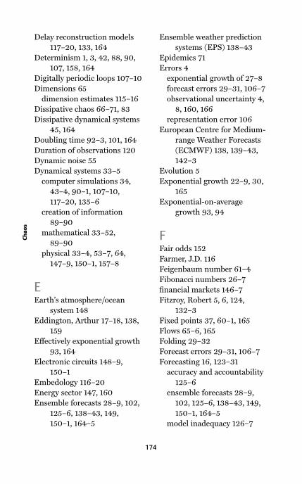
Delay reconstruction models

117–20, 133, 164

Determinism 1, 3, 42, 88, 90,

107, 158, 164

Digitally periodic loops 107–10

Dimensions 65

dimension estimates 115–16

Dissipative chaos 66–71, 83

Dissipative dynamical systems

45, 164

Doubling time 92–3, 101, 164

Duration of observations 120

Dynamic noise 55

Dynamical systems 33–5

computer simulations 34,

43–4, 90–1, 107–10,

117–20, 135–6

creation of information

89–90

mathematical 33–52,

89–90

physical 33–4, 53–7, 64,

147–9, 150–1, 157–8

EEarth’s atmosphere/ocean

system 148

Eddington, Arthur 17–18, 138,

159

Effectively exponential growth

93, 164

Electronic circuits 148–9,

150–1

Embedology 116–20

Energy sector 147, 160

Ensemble forecasts 28–9, 102,

125–6, 138–43, 149,

150–1, 164–5

Ensemble weather prediction

systems (EPS) 138–43

Epidemics 71

Errors 4

exponential growth of 27–8

forecast errors 29–31, 106–7

observational uncertainty 4,

8, 160, 166

representation error 106

European Centre for Medium-

range Weather Forecasts

(ECMWF) 138, 139–43,

142–3

Evolution 5

Exponential growth 22–9, 30,

165

Exponential-on-average

growth 93, 94

FFair odds 152

Farmer, J.D. 116

Feigenbaum number 61–4

Fibonacci numbers 26–7

financial markets 146–7

Fitzroy, Robert 5, 6, 124,

132–3

Fixed points 37, 60–1, 165

Flows 65–6, 165

Folding 29–32

Forecast errors 29–31, 106–7

Forecasting 16, 123–31

accuracy and accountability

125–6

ensemble forecasts 28–9,

102, 125–6, 138–43, 149,

150–1, 164–5

model inadequacy 126–7

174

Ch

ao

s

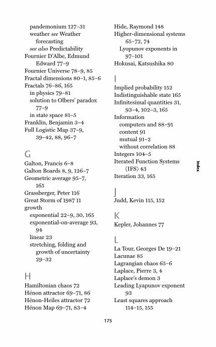
pandemonium 127–31

weather see Weather

forecasting

see also Predictability

Fournier D’Albe, Edmund

Edward 77–9

Fournier Universe 78–9, 85

Fractal dimensions 80–1, 85–6

Fractals 76–86, 165

in physics 79–81

solution to Olbers’ paradox

77–9

in state space 81–5

Franklin, Benjamin 3–4

Full Logistic Map 37–9,

39–42, 88, 96–7

GGalton, Francis 6–8

Galton Boards 8, 9, 126–7

Geometric average 95–7,

165

Grassberger, Peter 116

Great Storm of 1987 11

growth

exponential 22–9, 30, 165

exponential-on-average 93,

94

linear 23

stretching, folding and

growth of uncertainty

29–32

HHamiltonian chaos 72

Hénon attractor 69–71, 86

Hénon-Heiles attractor 72

Hénon Map 69–71, 83–4

Hide, Raymond 148

Higher-dimensional systems

65–72, 74

Lyopunov exponents in

97–101

Hokusai, Katsushika 80

IImplied probability 152

Indistinguishable state 165

Infinitesimal quantities 31,

93–4, 102–3, 165

Information

computers and 88–91

content 91

mutual 91–2

without correlation 88

Integers 104–5

Iterated Function Systems

(IFS) 43

Iteration 33, 165

JJudd, Kevin 115, 152

KKepler, Johannes 77

LLa Tour, Georges De 19–21

Lacunae 85

Lagrangian chaos 65–6

Laplace, Pierre 3, 4

Laplace’s demon 3

Leading Lyapunov exponent

93

Least squares approach

114–15, 155

175

Ind

ex

Leonardo of Pisa 25

LeVerrier, Urbain Jean Joseph

6, 57, 132–3

Limits 113

Linear dynamical systems 10,

28, 51, 156, 165

Linear growth 23

Logistic Map 45, 59–60, 92,

95, 155

attractors 46, 48–9

computer simulations

107–10

universality 60–4

Long-range modelling see

models

Lorenz, Ed 6, 66, 74, 133, 145,

148

Lorenz attractor 66, 67

Lorenz system 66–9, 101,

157–8

Lothar/T1 storm of 1999

142–3

Low-dimensional systems

58–64, 74

Lyapunov exponents 93–102,

157, 165–6

in higher dimensions 97–101

positive exponents with

shrinking uncertainties

101–2

Lyapunov time 166

MMacbeth 124–5

Mach, E. 53

Machete’s Moore-Spiegel

circuit 117, 118, 149, 150–1

Mandelbrot, Benoît 80, 86

Maps 23, 35–44, 166

see also under individual

types of map

Markets 146–7

Mathematical dynamical

systems 33–52, 89–90

attractors 35–9, 45–7

maps 35–44

parameters and model

structure 44–5

statistical models of Sun

spots 50–2

tuning model parameters

and structural stability

47–50

Mathematical fractals 76, 77

Mathematical models 15,

58–75

delay equations 71

dissipative chaos 66–71

exploiting insights of chaos

73–5

Hamiltonian chaos 72

higher-dimensional systems

65–72, 74

origin of mathematical term

‘chaos’ 65

universality 60–4

Mathematics 20–1, 34, 55–6,

159

Maximum likelihood 115

Maxwell, James Clerk 8–9

May, Lord 58–60

Medical research 71

Mercury 57

Meteorology see Weather

forecasting

Middle Thirds Cantor set 77,

85–6

176

Ch

ao

s

Middle Thirds IFS Map 43,

81–3

Model inadequacy 57, 111,

126–7, 130–1, 152–3, 160

Models 16, 27, 132–53, 166

climate 143–6, 159–60

data-based 117–20, 132–4

mathematical see

Mathematical models

odds and probabilities

149–53

parameters see Parameters

Phynance 146–7

physical systems 147–9,

150–1

simulation 135–7

weather forecasting 12–16,

135–43

Moore-Spiegel attractor 67,

69–71

Moore-Spiegel system 117, 118,

149, 150–1

Moran-Ricker Map 41, 59, 60,

64, 95–6

Mutual information 91–2

NNAG (Not A Galton) Board

127–31

Neptune 57

New Zealand 143

Newton, Isaac 73, 79

Newton’s Laws 3

Night sky, darkness of 77–9

Noise 53–4, 166

dynamic 55

exponential error growth

27–8

observational 4, 55–7, 92,

106, 111

Noise model 54, 92, 105, 111,

166

Noise reduction 29

Non-constructive proof 46,

166

Nonlinearity 1, 10, 60, 155,

159–60, 166

model parameter estimation

114–15

Numbers 104–5, 155–6

Numerical weather prediction

(NWP) models 135–7

OObservational noise 4, 55–7,

92, 106, 111

Observational uncertainty 4, 8,

160, 166

Observations 105–7

duration of 120

and model states 154

operational weather

forecasting 12–15

Odds 149–53

Olbers’ paradox 77–9

Osceledec, V. 93

PPackard, N.H. 116

Pandemonium 127–31, 166

Parameters 24, 166

best values for 113–15, 154–5

and model structure 44–5

tuning 47–50

Perfect Model Scenario (PMS)

54, 56, 57, 114, 122, 166

177

Ind

ex

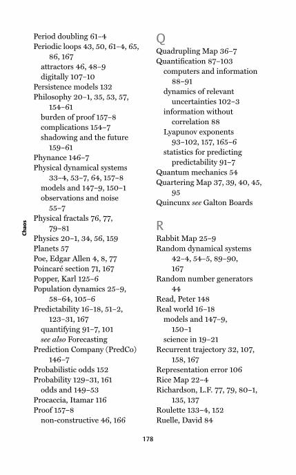
Period doubling 61–4

Periodic loops 43, 50, 61–4, 65,

86, 167

attractors 46, 48–9

digitally 107–10

Persistence models 132

Philosophy 20–1, 35, 53, 57,

154–61

burden of proof 157–8

complications 154–7

shadowing and the future

159–61

Phynance 146–7

Physical dynamical systems

33–4, 53–7, 64, 157–8

models and 147–9, 150–1

observations and noise

55–7

Physical fractals 76, 77,

79–81

Physics 20–1, 34, 56, 159

Planets 57

Poe, Edgar Allen 4, 8, 77

Poincaré section 71, 167

Popper, Karl 125–6

Population dynamics 25–9,

58–64, 105–6

Predictability 16–18, 51–2,

123–31, 167

quantifying 91–7, 101

see also Forecasting

Prediction Company (PredCo)

146–7

Probabilistic odds 152

Probability 129–31, 161

odds and 149–53

Procaccia, Itamar 116

Proof 157–8

non-constructive 46, 166

QQuadrupling Map 36–7

Quantification 87–103

computers and information

88–91

dynamics of relevant

uncertainties 102–3

information without

correlation 88

Lyapunov exponents

93–102, 157, 165–6

statistics for predicting

predictability 91–7

Quantum mechanics 54

Quartering Map 37, 39, 40, 45,

95

Quincunx see Galton Boards

RRabbit Map 25–9

Random dynamical systems

42–4, 54–5, 89–90,

167

Random number generators

44

Read, Peter 148

Real world 16–18

models and 147–9,

150–1

science in 19–21

Recurrent trajectory 32, 107,

158, 167

Representation error 106

Rice Map 22–4

Richardson, L.F. 77, 79, 80–1,

135, 137

Roulette 133–4, 152

Ruelle, David 84

178

Ch

ao

s

SSample-statistics 113, 167

Self-similarity 76–7, 78

Sensitive dependence 1–2, 5–6,

8–10, 15, 94, 107, 158,

167

Shadowing 111, 125, 156,

159–61, 167

Sharkovski, A.N. 65

Shift Map 40, 95, 96

Short-range forecasting see

Forecasting

Simulation models 135–7

Small differences see Sensitive

dependence

Smith, Henry 77

Solar eclipse 17–18, 73,

138–9

Solar system 73

Spiegel, Ed 127

State 36, 167

State space 36, 168

fractals in 81–5

Statistical self-similarity 76–7

Statistics 20–1, 35, 112–22

applied statistics 122

best values for parameters

113–15

dimension estimates 115–16

limits of 113

models of Sun spots 50–2

for predicting predictability

91–7

surrogate data 121

Takens’ Theorem 55, 116–20,

133

Stochastic systems 42–4, 54–5,

89–90, 167

Stock markets 146–7

Storms 6

Burns’ Day storm 10–16,

139–42

Great Storm of 1987 11

T1/Lothar Storm of 1999

142–3

Strange accumulators 85

Strange attractors 84–5,

168

Stretching 29–32

Strict self-similarity 76, 78

Structural stability 47–50

Sun spots 50–2

Superposition 51

Surrogate data 121

Sustainable odds 152–3

TT1/Lothar Storm of 1999

142–3

Takens, Floris 84

Takens’ Theorem 55, 116–20,

133

Tent Map 41, 95, 96

Time series 25, 34–5, 168

Transient dynamics 43–4,

127–31, 168

Tripling Tent Map 40, 81–3,

95, 96

Turbulence 84

UUeda, Yoshisuke 73

UK Meteorological Office 6

Uncertainty 2

in current state, parameters

and model structure

47–50

179

Ind

ex

evolution in Lorenz system

66–9

evolution in Yule Map 51–2

exponential growth 24, 28

quantifying dynamics of see

Quantification

sensitivity and 8–10

stretching, folding and

growth of 29–32

Universality 60–4

VVulcan 57

WWeather forecasting 3–4, 6–16,

17–18, 106, 135–43, 147

Burns’ Day storm 10–16,

139–42

ensemble prediction systems

138–43

the first forecasts 6–10,

80

numerical weather

prediction models

135–7

operational weather

forecasting 12–15

Whitehead, Alfred North 16,

17

YYule, Udny 50–1, 88

Yule Map 51–2

180

Ch

ao

s