Chaos and Unpredictability in Evolution

Iaroslav Ispolatov1, ∗ and Michael Doebeli2, †

1 Departamento de Fisica, Universidad de Santiago de Chile, Casilla 302, Correo 2, Santiago, Chile2Department of Zoology and Department of Mathematics, University of British Columbia,

6270 University Boulevard, Vancouver B.C. Canada, V6T 1Z4

The possibility of complicated dynamic behaviour driven by non-linear feedbacks in dynamical systems hasrevolutionized science in the latter part of the last century. Yet despite examples of complicated frequencydynamics, the possibility of long-term evolutionary chaos is rarely considered. The concept of “survival ofthe fittest” is central to much evolutionary thinking and embodies a perspective of evolution as a directionaloptimization process exhibiting simple, predictable dynamics. This perspective is adequate for simple scenarios,when frequency-independent selection acts on scalar phenotypes. However, in most organisms many phenotypicproperties combine in complicated ways to determine ecological interactions, and hence frequency-dependentselection. Therefore, it is natural to consider models for the evolutionary dynamics generated by frequency-dependent selection acting simultaneously on many different phenotypes. Here we show that complicated,chaotic dynamics of long-term evolutionary trajectories in phenotype space is very common in a large class ofsuch models when the dimension of phenotype space is large, and when there are epistatic interactions betweenthe phenotypic components. Our results suggest that the perspective of evolution as a process with simple,predictable dynamics covers only a small fragment of long-term evolution. Our analysis may also be the firstsystematic study of the occurrence of chaos in multidimensional and generally dissipative systems as a functionof the dimensionality of phase space.

Keywords: Evolution, Adaptive dynamics, Chaos

I. AUTHOR SUMMARY

40 years ago, the discovery of deterministic chaos has rev-olutionized science. Surprisingly, few of these insights haveentered the realm of evolutionary biology, where survival ofthe fittest epitomizes evolution as an optimization process thatgenerally converges to an equilibrium, the optimal phenotype.This perspective may be correct for simple phenotypes, suchas body size, but in reality, all organisms have a multitude ofphenotypic properties that impinge on birth and death rates,and hence on evolutionary dynamics. However, evolution inhigh-dimensional phenotype spaces is rarely studied due tothe formidable technical difficulties involved. In the enclosedpaper, we have used the recently developed mathematicalframework of adaptive dynamics for a systematic investiga-tion of long-term evolutionary dynamics in high-dimensionalphenotype spaces. Our main conclusions are that chaotic evo-lution is common in complicated phenotype spaces. This isrelevant for Gould’s famous question about “replaying thetape of life”: if evolution is fundamentally chaotic, then evo-lution is generally unpredictable in the long term, even if se-lection is deterministic. Our results show that evolutionarychaos is indeed common, and hence unpredictability is therule rather than the exception. This suggests that the perspec-tive of evolution as an equilibrium process must be fundamen-tally revised.

∗Electronic address: jaros007@gmail.com†Electronic address: doebeli@zoology.ubc.ca

II. INTRODUCTION

Evolution generally takes place in complex ecosystems andis affected by many different processes that generate non-linear dependencies. According to general dynamical sys-tems theory, which has shown that even simple dynamicalsystem can exhibit complicated dynamics [2, 16, 26, 27], onewould therefore expect that evolutionary dynamics tend to becomplicated. However, this is contrary to traditional evolu-tionary thinking, which is based on the concept of “survivalof the fittest”, and on metaphors of static fitness landscapes[12, 33, 36], in which evolution optimizes simple, scalar phe-notypes such as body size, age and size at maturity, fecun-dity, stress tolerance, antibiotic resistance, etc. Accordingly,the “fittest” type wins, and hence evolution is often envi-sioned as a dynamical system that converges to an equilib-rium in phenotype space, representing the optimally adaptedtype. It is of course generally acknowledged that over largetime scales, evolution is a non-stationary process, but this isusually attributed to long-term changes in the external envi-ronment causing shifts in evolutionary optima.

Static fitness landscapes describe frequency-independentselection whose strength and direction is not affected by thecurrent phenotypic composition of an evolving population.However, it is widely recognized that ecological interactions,such as competition and predation, often lead to frequency-dependent selection, in which the current phenotypic compo-sition of a population determines whether a particular pheno-type is advantageous or not [8, 18, 30]. For example, whetherit is advantageous to have a preference for a particular type offood depends on the preferences of the other individuals in thepopulation. Frequency dependence generates an evolutionaryfeedback loop, because selection pressures, which cause evo-lutionary change, change themselves as a population’s pheno-

arX

iv:1

309.

6261

v1 [

q-bi

o.PE

] 2

4 Se

p 20

13

2

type distribution evolves. It is well-known that this feedbackcan produce complicated dynamics in models in which thedynamic variables are the frequencies of a fixed and finite setof different types in a given population [1, 13, 28, 29, 31].However, such models are essentially ecological models, inwhich chaotic dynamics is the result of coexistence of dif-ferent types due to frequency-dependent selection. They areecological models because they describe the dynamics of the(relative) abundance of different types on short, ecologicaltime scales. In particular, the phenotypes or genotypes presentin the population never go beyond the finite set initially pro-vided by the model. Perhaps this essentially ecological natureof these models helps explain why, even though such modelshave been shown to exhibit complicated dynamics, the pos-sibility of evolutionary chaos does not really play a role inmainstream evolutionary thinking.

It is important to distinguish models for short-term fre-quency dynamics from evolutionary models in which the dy-namic variables are the (mean) phenotypes themselves, andwhich track the trajectories of such phenotypes in continuousphenotype spaces and over long evolutionary time scales. Thephase space for this type of model is the space of all possiblephenotypes (rather than the space of frequencies of differenttypes). Adaptive dynamics [6, 14] provides a useful frame-work for generating models of long-term evolutionary dynam-ics of phenotypes. Intuitively, adaptive dynamics unfolds as aseries of phenotypic substitutions that give rise to evolution-ary trajectories in phenotype space. Frequency dependenceplays an important role in adaptive dynamics, but most often,this feedback mechanism has been studied in relatively simplescenarios, in which frequency dependence is still generally ex-pected to generate long-term equilibrium dynamics. But evenin simple phenotype spaces, frequency dependence can lead tointeresting evolutionary phenomena, such as adaptive diversi-fication [8, 9, 14]. In more complicated phenotype spaces con-taining scalar phenotypes of each of a number of co-evolvingpopulations, frequency dependence can generate complicatedevolutionary dynamics. For example, coevolution of scalartraits in predator and prey populations can lead to arms racesin the form of cyclic dynamics in phenotype space [3, 6, 7],and coevolution of scalar traits in a three-species food chaincan generate chaotic dynamics in phenotype space [4]. In allthese examples, the dynamic variables undergoing evolutionare the (mean) traits in the various interacting species, and thetrajectories of these traits in combined phenotype space com-prising the scalar traits of all interacting species can exhibitcomplicated dynamics.

Long-term evolutionary dynamics of continuous pheno-types is ultimately driven by birth and death rates of individ-ual organisms. In general, these birth and death rates are de-termined in a complicated way by many different phenotypicproperties, which could be as diverse as the molecular effi-ciency of photosynthesis and the height of trees. Therefore,even for single species it is natural to study evolutionary dy-namics in high-dimensional phenotype spaces. For frequency-independent selection, evolution is still an optimization pro-cess in such spaces, although genetic correlations betweenphenotypic components may warp the fitness landscape and

alter the convergence dynamics to the local optima [24]. Yet,apart from a few examples [10, 35], little is known about theexpected complexity of the long-term evolutionary dynamicsof high-dimensional phenotypes when selection is frequency-dependent. Here we ask whether frequency dependence dueto competition in high-dimensional phenotype spaces of sin-gle species yields evolutionary dynamics that are fundamen-tally different from the equilibrium dynamics resulting fromevolution in simple phenotype spaces.

III. MODEL AND RESULTS

We use adaptive dynamics theory [6, 14] to study the long-term evolutionary dynamics in a large class of multidimen-sional single-species competition models. The starting pointis the widely used logistic model [8]

∂N(x, t)

∂t= rN(x, t)

1−

∫α(x, y)N(y, t)dy

K(x)

. (1)

Here N(x, t) is the density of individuals of phenotypex at time t, and K(x) is the carrying capacity of amonomorphic population consisting entirely of x-individuals.The competitive impact between individuals of pheno-types x and y is given by the competition kernel α(x, y),so that an x-individual experiences an effective density∫α(x, y)N(y, t)dy. This model has been used extensively

to study the evolutionary dynamics of scalar traits x ∈ R[8]. Here we assume more generally that x ∈ Rd is a d-dimensional vector describing d ≥ 1 scalar phenotypic prop-erties. We also assume that α(x, x) = 1 for all x, and thatthe intrinsic growth rate r is independent of the phenotype xand is equal to 1. To derive the adaptive dynamics of the mul-tidimensional trait x, we consider a resident population thatis monomorphic for trait x, for which the ecological model(1) has a unique, globally stable equilibrium density K(x),regardless of the dimension d of x. Assuming that the resi-dent is at its ecological equilibrium K(x), the invasion fitnessf(x, y) of a rare mutant y is its per capita growth rate in theresident population x,

f(x, y) = 1− α(y, x)K(x)

K(y). (2)

The selection gradient s(x) = (s1(x), . . . , sd(x)) is derivedfrom the invasion fitness as

si(x) =∂f(y, x)

∂yi

∣∣∣∣y=x

= − ∂α(y, x)

∂yi

∣∣∣∣y=x

+∂K(x)

∂xi

1

K(x).

(3)Finally, the adaptive dynamics of the trait x is

dx

dt=M(x) · s(x), (4)

where M(x) is a d× d-matrix describing the mutational pro-cess in the d phenotypic components [8, 25] (and where dx/dt

3

and s(x) are column vectors). In general, the entries of M(x)depend on the current population size, and hence implicitlyon x, but for simplicity we assume here thatM(x) is the iden-tity matrix, which is a conservative assumption as far as thecomplexity of the adaptive dynamics (4) is concerned.

Complicated dynamics in the form of oscillations can al-ready occur if the selection gradient s(x) in (4) is linear. Infact, with randomly chosen coefficients, the probability of os-cillatory behaviour is 1 − 2−d(d−1)/4, and hence rapidly ap-proaches 1 as the dimension of phenotype space is increased[11]. To study non-linear systems, we assume that the com-plexity of the interactions between phenotypic components indetermining ecological properties is contained in the compe-tition kernel α(x, y) : Rd × Rd → R, which is in general acomplicated, nonlinear function that reflects epistatic interac-tions between the different phenotypic components. We onlyconsider the Taylor expansion of this function up to quadraticterms, and absorbing constant terms into a change of coordi-nates, we get

∂α(y, x)

∂yi

∣∣∣∣y=x

≈ −d∑j=1

bijxj −d∑

j,k=1

aijkxjxk (5)

For the carrying capacity, we assume a simple symmetricform: K(x) = exp(−

∑i x

4i /4), which, together with the

competition kernel gradient (5), ensures that the trajectoriesof the adaptive dynamics (4) are confined to a finite region ofphenotype space. With these assumptions, the adaptive dy-namics (4), describing the evolution of the multidimensionalphenotype x, becomes

dxidt

=

d∑j=1

bijxj +

d∑j,k=1

aijkxjxk − x3i , i = 1, . . . , d. (6)

The parameters bij and aijk reflect the epistatic interactionsamong the d phenotypic components. If bij = 0 for i 6= j andaijk = 0 for i 6= j, k, there is no epistasis between the phe-notypic components, and in that case, the adaptive dynamics(6) always converges to an equilibrium in phenotype space.Thus, if system (6) exhibits complicated dynamics, it must bedue to epistatic interactions. To address the question of theubiquity of complex evolutionary dynamics, we chose, for agiven dimension d of phenotype space, many different setsof parameters bij and aijk, reflecting a wide range of possibleepistatic interaction structures for the phenotypic components.Specifically, parameters were drawn randomly from a Gaus-sian distribution with mean zero and variance 1, and for eachchoice of parameters evolutionary trajectories were obtainedby integrating the adaptive dynamics (6) numerically startingfrom a random initial condition. We show in section C of theMethods that the results are qualitatively the same for any dis-tribution of the coefficients bij and aijk with a finite variance,and that the results remain true if the coefficients are rescaledsuch the total strength of epistatic interactions is independentof the dimension d of phenotype space. For each trajectorywe measured the time average of the largest Lyapunov ex-ponent λ [5] (see Methods). Based on Lyapunov exponents,we classified the evolutionary trajectories into three groups:

-2 0 2-2

0

2

-10 0 10

-10

0

10

-10 0 10

-10

0

10

-100 0 100

-100

0

100

x1

x2

x1

x1 x1

x2

x2 x2

Figure 1

a) b)

c) d)

FIG. 1: a) Example of equilibrium dynamics for d = 5; largest Lya-punov exponent λ = −0.12. b) Example of quasi-periodic dynamicsfor d = 15; largest Lyapunov exponent λ = 0.008. c) Example ofchaotic dynamics on a non-ergodic (“strange”) attractor for d = 15;largest Lyapunov exponent λ = 1.35. d) Example of ergodic chaoticdynamics for d = 100; largest Lyapunov exponent λ = 1850. Thetrajectory essentially fills the phenotype space on a scale of (−d, d)in each phenotypic dimension. Here and below the integration of (6)was performed from t = 0 to t = 400/d2 using a 4th-order Runge-Kutta method with time step dt = 0.1d−2. The coefficients aij andbijk were randomly drawn from a Gaussian distribution with zeromean and unit variance, and the initial conditions were randomlydrawn from a Gaussian distribution with mean 0 and variance d2.The panels show projections of the evolutionary trajectories onto arandomly chosen 2-dimensional subspace of the phenotype space.

fixed points (λ < −0.1), periodic or quasi-periodic attractors(|λ| < 0.1), and chaotic attractors (λ > 0.1). Examples areshown in Fig. 1.

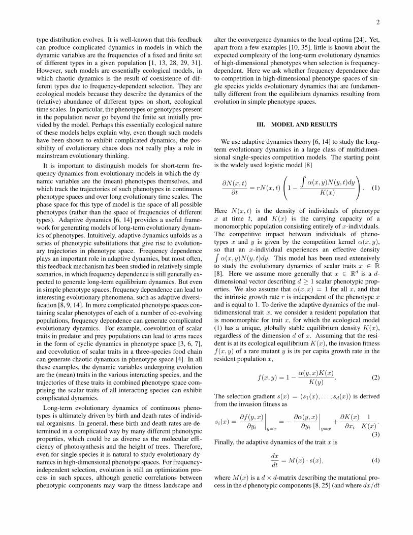
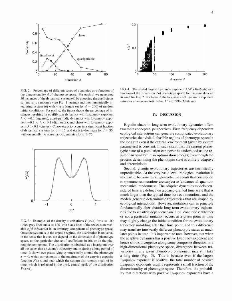
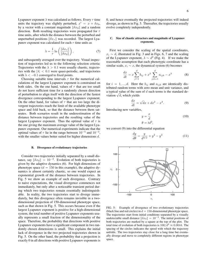
Our main result is that the probability of chaos increaseswith the dimensionality d of the evolving system, approach-ing 1 for d ∼ 75 (Fig. 2). Moreover, already for d & 15, themajority of chaotic trajectories become ergodic [5], and henceessentially fill out the available phenotype space over evolu-tionary time. The size of the filled phenotype space scalesapproximately as |xi| < d for each phenotypic dimension i(Methods), and the density of trajectories exhibits a universalprobability distribution (Fig. 3). It is important to note thatbecause these ergodic trajectories fill out large areas of phe-notype space, they are very different from noisy equilibriumpoints. Finally, we observe that the largest Lyapunov expo-nent converges to the universal asymptotic λ ∼ d2 (Fig. 4).In Methods we provide qualitative analytical explanations forthese numerical results. In particular, we derive an analyticalapproximation for the probability of chaos as a function of thedimension of phenotype space (Fig. 9) by arguing that a tra-jectory is chaotic if all fixed points of system (6) have at leastone repelling direction, which becomes certain for large d dueto the epistatic interactions between phenotypic components.

4

0 20 40 60 80dimension d

0

0.2

0.4

0.6

0.8

1Pr

obab

ility

chaos

fixed pointquasiperiodic

Figure 2

FIG. 2: Percentage of different types of dynamics as a function ofthe dimensionality d of phenotype space. For each d, we generated50 instances of the dynamical system (6) by choosing the coefficientsbij and aijk randomly (see Fig. 1 legend) and then numerically in-tegrating system (6) with 4 sets (single set for d = 200) of randominitial conditions. For each d, the figure shows the percentage of in-stances resulting in equilibrium dynamics with Lyapunov exponentλ < −0.1 (squares), quasi-periodic dynamics with Lyapunov expo-nent −0.1 < λ < 0.1 (diamonds), and chaos with Lyapunov expo-nent λ > 0.1 (circles). Chaos starts to occur in a significant fractionof dynamical systems for d ≈ 15, and starts to dominate for d ≈ 35,with essentially no non-chaotic dynamics for d ≥ 75.

-1 0 1x/d

0

1

P(x/

d)

Figure 3

FIG. 3: Examples of the density distributions P (x/d) for d = 100(thick grey line) and d = 150 (thin black line) of the scaled state vari-able x/d (Methods) in an arbitrary component of phenotype space.Once the system is in the ergodic regime, the distribution is universalin the sense that it does not depend on the dimension d of phenotypespace, on the particular choice of coefficients in (6), or on the phe-notypic component. The distribution is obtained as a histogram overall the states that a system’s trajectory attains during a long period oftime. It shows two peaks lying symmetrically around the phenotypex = 0, which corresponds to the maximum of the carrying capacityfunction K(x), and near which the system also spends much of itstime, which is reflected in the third, central peak of the distributionP (x/d).

0 50 100 150 200dimension d

0

0.1

0.2

λ/d

2

Figure 4

FIG. 4: The scaled largest Lyapunov exponent λ/d2 (Methods) as afunction of the dimension d of phenotype space, for the same data setas used for Fig. 2. For large d, the largest scaled Lyapunov exponentsaturates at an asymptotic value λ∗ ≈ 0.235 (Methods).

IV. DISCUSSION

Ergodic chaos in long-term evolutionary dynamics offerstwo main conceptual perspectives. First, frequency-dependentecological interactions can generate complicated evolutionarytrajectories that visit all feasible regions of phenotype space inthe long run even if the external environment (given by systemparameters) is constant. In such situations, the current pheno-typic state of a population can never be understood as the re-sult of an equilibrium or optimisation process, even though theprocess determining the phenotypic state is entirely adaptiveand deterministic.

Second, chaotic evolutionary trajectories are intrinsicallyunpredictable. At the very basic level, biological evolution isstochastic, because the single-molecule events that correspondto spontaneous mutations are subject to fundamental, quantummechanical randomness. The adaptive dynamics models con-sidered here are defined on a coarse-grained time scale that ismuch larger than the typical time between mutations, and themodels generate deterministic trajectories that are shaped byecological interactions. However, mutations can in principlefundamentally alter chaotic long-term evolutionary trajecto-ries due to sensitive dependence on initial conditions: whetheror not a particular mutation occurs at a given point in timemay slightly change the initial condition for the evolutionarytrajectory unfolding after that time point, and this differencemay translate into vastly different phenotypic states at muchlater points in time. It is important to note, however, that whenthe adaptive dynamics has a positive Lyapunov exponent andhence shows divergence along some composite direction in ahigh-dimensional phenotype space, divergence between tra-jectories in any given phenotypic component may still takea long time (Fig. 5). This is because even if the largestLyapunov exponent is positive, the total number of positiveLyapunov exponents usually represents a small fraction of thedimensionality of phenotype space. Therefore, the probabil-ity that directions with positive Lyapunov exponents have a

5

significant component in two randomly chosen dimensions issmall, which explains the initial lack of divergence in the twoprojected trajectories shown in Fig. 5. On the other hand, theprobability that a projection is exactly 0 in all directions withpositive Lyapunov exponents is 0, and hence divergence willeventually occur. Extrapolating from this, replaying the tapeof life [17] could potentially result in completely different out-comes if evolution is chaotic.

Our results are also relevant for the general problem of theprevalence of chaos in multidimensional dynamical systems.Chaos is well studied in high-dimensional Hamiltonian sys-tems [37], as well as in discrete-time systems of coupled oscil-lators with many degrees of freedom [20, 21], but these resultsare not applicable to dissipative, non-Hamiltonian systems incontinuous time, such as the adaptive dynamics models stud-ied here. Surprisingly, our analysis may be the first systematicstudy of the occurrence of chaos in such systems as a functionof the dimensionality of phase space.

Because the likelihood of chaotic evolutionary dynamicsin our models is strongly influenced by the dimensionality ofphenotype space, the biological relevance of our results hingeson the number of phenotypic properties affecting ecologicalinteractions in real systems, and on the potential for epistasisbetween these phenotypic properties. Given that metabolicnetworks of even the simplest bacterial organisms such as E.coli are incredibly complex [22, 32], it seems likely that ingeneral, many phenotypic properties combine in complicatedways to affect ecological interactions such as competition forresources. Data testing this directly seems to be scant, butan indication for high-dimensionality of ecologically relevantphenotype space comes for example from studies of the ge-netics of adaptive diversification in fishes [23] and in bacte-ria [19]. In pairs of fish species that have recently speciatedinto two different ecotypes, there is abundant genetic differ-entiation between the species, which is distributed over thewhole genome. Some of this differentiation is due to differ-ences in mating preferences, but it appears that many of theobserved genetic differences are related to ecological traits,and hence that many different genes affect ecological proper-ties, and thus ecological interactions, of these fish [23]. Simi-larly, a genetic analysis of adaptive diversification in evolutionexperiments with E. coli revealed that the diversified ecotypesthat evolved from a single ancestral strain in ca. 1000 gen-erations differed in many genes carrying adaptive mutations[19]. Other recent evolution experiments with E. coli showedthe importance of epistasis for evolutionary dynamics [34]. Itwould seem to be an important empirical endeavour to gain ageneral understanding of the number of different phenotypicproperties that can be expected to affect ecological interac-tions, and of the degree of epistasis between them.

Even if one accepts the premise of high-dimensional phe-notype spaces, one could question the realism of the logisticcompetition models used here. While it is true that our modelsdo not derive from an underlying mechanistic model for eco-logical interactions between individual organisms, our statisti-cal approach examines in some sense all possible competitionmodels whose trajectories are confined to a bounded region inphenotype space. This is because, to second order, any such

model for the evolutionary dynamics of d phenotypic compo-nents will have the general form (6). In particular, the subsetof “realistic” models will have this form. Thus, if essentiallyall models of the form (6) have chaotic dynamics for high d,then any particular realistic model is likely to have such dy-namics as well.

For now, our results warrant at least a critical re-examination of the generality of simple equilibrium and op-timization dynamics in evolution. 40 years ago, the real-ization that simple ecological models can have very compli-cated dynamics revolutionized ecological thinking [27]. Ourhigh-dimensional models are not simple, but they show thatnon-linear evolutionary feedbacks generated by frequency-dependent ecological interactions can also lead to very com-plicated dynamics. In fact, with frequency dependence mostevolutionary dynamics may be chaotic when phenotypes arehigh-dimensional. In general, evolution is a complicated dy-namical systems driven by birth and death events that are de-termined by many different factors, such as external bioticand abiotic conditions, current phenotype distributions, ageand physiological condition, etc. If birth and death rates arecomplicated functions of many different factors that changethemselves as evolution unfolds, we do not see any reason toexpect that in general, evolutionary dynamics should be sim-ple (after all, it is for example well known that weather oftenexhibits chaos and long-term unpredictability, essentially be-cause of the nonlinearity of the dynamics and the complexityof the interactions between the many different components de-termining the weather). Nevertheless, our perception is that todate, evolutionary biologists are unaware of the fact that gen-eral evolutionary dynamics in continuous phenotype spaces ofhigh dimensions are likely to be very complicated. Knowingthat, in principle, long-term evolutionary complexity can bedue to intrinsic frequency-dependent interactions rather thansimply to changes in the external environment would gener-ally seem to be useful, in the same way as it was useful when,four decades ago, ecologists became aware of the possibil-ity of chaos due to non-linear interactions in generic ecolog-ical models. Our results indicate that chaos and complexityin long-term evolutionary dynamics should be given seriousconsideration in future studies.

V. METHODS

Here we describe how the largest Lyapunov exponent is cal-culated, illustrate the divergence of chaotic trajectories, andprovide approximate analytical explanations for the numeri-cal results reported for the size of chaotic attractors (Figure2), the probability of chaos as a function of the dimension dof phenotype space (Figure 3), and the scaling of the largestLyapunov exponent with d (Figure 4).

A. Calculation of Lyapunov exponents

For each trajectory obtained through numerical integrationof the adaptive dynamics (6), the time average of the largest

6

Lyapunov exponent λwas calculated as follows. Every τ timeunits the trajectory was slightly perturbed, x′ = x + δx0,by a vector with a constant magnitude ‖δx0‖ and a randomdirection. Both resulting trajectories were propagated for τtime units, after which the distance between the perturbed andunperturbed positions ‖δxτ‖ was recorded. The largest Lya-punov exponent was calculated for each τ time units as

λ =1

τln

(‖δxτ‖‖δx0‖

), (7)

and subsequently averaged over the trajectory. Visual inspec-tion of trajectories led us to the following selection criteria:Trajectories with the λ > 0.1 were usually chaotic, trajecto-ries with the |λ| < 0.1 were quasi-periodic, and trajectorieswith λ < −0.1 converged to fixed points.

Choosing suitable time intervals τ for the numerical cal-culations of the largest Lyapunov exponent is constrained onboth sides. On the one hand, values of τ that are too smalldo not leave sufficient time for a randomly chosen directionof perturbation to align itself with the direction of the fastestdivergence corresponding to the largest Lyapunov exponent.On the other hand, for values of τ that are too large the di-vergent trajectories reach the limit of the available phenotypespace and fold back, so that the distance between them sat-urates. Both scenarios result in the underestimation of thedistance between trajectories and the resulting value of thelargest Lyapunov exponent. Thus the optimal value of τ isthe one giving the maximum average value of the largest Lya-punov exponent. Our numerical experiments indicate that theoptimal values of τ lie in the range between 10−5 and 10−3,with the smaller values better suited for higher dimensions d.

B. Divergence of evolutionary trajectories

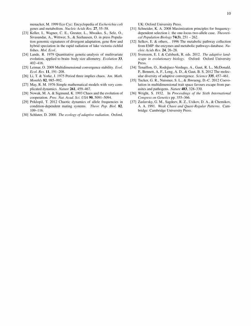
Consider two trajectories initially separated by a small dis-tance, say ‖δx0‖ = 10−3. Evolution of both trajectories isgiven by the adaptive dynamics (6). For high dimensions ofphenotype space (d = 150 in this example), the adaptive dy-namics is almost certainly chaotic, so one would expect anexponential growth of the distance between trajectories. InFig. 5 we show an example of such divergence. Contraryto naive expectations, the visual divergence commences notimmediately, but only after a noticeable transient period dur-ing which two trajectories remain essentially indistinguish-able. In reality, the two trajectories start to diverge imme-diately, but this divergence often remains invisible in a two-dimensional projection of 150-dimensional phenotype space,such as that shown in Fig. 5. This occurs because even if thelargest Lyapunov exponent is positive for a high-dimensionalsystem, the total number of positive Lyapunov exponents usu-ally represents a small fraction of the dimensionality of thespace. Therefore, the probability that directions with positiveLyapunov exponents have a significant component in two ran-domly chosen dimensions is small. This explains the initiallack of divergence in the two projected trajectories shown inFig. 5. On the other hand, the probability that a projection isexactly 0 in all directions with positive Lyapunov exponents is

0, and hence eventually the projected trajectories will indeeddiverge, as shown in Fig. 5. Thereafter, the trajectories usuallyevolve completely independently.

C. Size of chaotic attractors and magnitude of Lyapunovexponents.

First we consider the scaling of the spatial coordinates,xi ∼ d, illustrated in Fig. 3 and in Figs. 6, 7 and the scalingof the Lyapunov exponent, λ ∼ d2 (Fig. 4). If we make thereasonable assumption that each phenotypic coordinate has asimilar scale, xi ∼ x, the dynamical system (6) becomes

dx

dt= x

d∑j=1

bij + x2d∑

j,k=1

aijk − x3 (8)

for i = 1, ..., d. Here the bij and aijk are identically dis-tributed random terms with zero mean and unit variance, anda typical value of the sum of d such terms is the standard de-viation

√d, which yields

dx

dt=√dx+ dx2 − x3. (9)

Introducing new variables,

y =x

d(10)

θ = td2,

we convert (9) into the differential equation

dy

dθ=

y

d3/2+ y2 − y3 (11)

-100 0 100

-100

0

100

x1

x2

FIG. 5: Example of divergence of two evolutionary trajectories(black line and red circles) in d = 150-dimensional phenotype space.The trajectories start from initial conditions separated by a visuallyundetectable small distance ‖δx0‖ = 10−3. The initial positions ofboth trajectories are marked by a square at the top of the plot. Thetotal time of evolution of both trajectories is 100/d2 ≈ 0.0044. Thespacing of the circles indicates the speed with which the trajectoryunfolds. The two trajectories stay close for a long time but eventu-ally diverge and move to completely different regions in phenotypespace.

7

0 50 100 150 200dimension d

0.2

0.4

0.6

0.8

1<x

2 >1/

2 /d

FIG. 6: Scaling of the mean square of a coordinate xi with the di-mensionality of phenotype space,

√〈x2i 〉 ∼ d. Same data set as used

for Fig. 2.

-100

0

100

200

2000100-200-200

100

x2

x1

FIG. 7: Examples of projections of ergodic chaotic trajectories ford = 15 (magenta), d = 30 (blue), d = 50 (dark blue), d = 75(yellow), d = 100 (green), d = 150 (red), and d = 200 (black). Thefigure illustrates the scaling xi ∼ d.

with two universal, d-independent terms and a linear term thatvanishes in the limit of large d � 1. The transformation (10)explains the observed scaling of the size of chaotic attractors,x = yd (Figs. 3, 6, 7), and of the largest Lyapunov expo-nent, whose dimension is the inverse of time, 1/t = d2/θ(Fig. 4). The transformation also shows that the linear term∑dj=1 bijxj in (6) does not produce any significant effect on

the probability of chaos and on the form of the attractor forlarge d.

Taking into account (9,10), it is possible to rescale the co-efficients bij and aijk in such a way that the total “strength”of epistatic interactions between the phenotypic components,as well as the size of the area of phenotype space filled outby ergodic trajectories, do not depend on the dimension d ofphenotype space. Eq. (6) with bij and aijk drawn from Gaus-sian distributions with variances 1/d and 1/d2 (so that theirtypical values are 1/

√d and 1/d) produces similar-sized er-

-1

0

1

2

201-2-2

1

x2

x1

FIG. 8: Examples of projections of ergodic chaotic trajectories sys-tem (6) (main text) when the coefficients bij and aijk were dividedby√d and d, respectively; d = 75 (red), and d = 100 (black).

godic attractors for various d, as shown in Fig. 8. A slightasymmetry of the trajectories in Fig. 8 is caused by the linearterms bij which are no longer irrelevant. Without these termsthe high-d trajectories of the rescaled Eq. (6) are completelyanalogous to the trajectories of the original Eq. (6) when thelatter are rescaled through division by d.

D. Probability of chaos.

Second, we provide an explanation for the increase in theoccurrence of chaos with the dimension d of phenotype space.Stationary points of the adaptive dynamics (6) are defined assolutions of the corresponding system of algebraic equationswhere the right-hand side is set equal to zero. Generally, asystem of d third-order algebraic equations has 3d solutions(some of which may coincide), and hence the dynamical sys-tem (6) has 3d stationary points. We propose that the systemis chaotic if all these stationary points are unstable in at leastone direction, i.e., if at least one eigenvalue of the local Jaco-bian matrix J at each stationary point x∗ has a positive realpart. If Pn is the probability that the real part of an eigen-value is negative, and assuming that all Jacobian eigenvaluesare statistically independent, the probability that at least oneout of d eigenvalues of the Jacobian at a stationary point has apositive real part is 1− P dn . Hence the probability of chaos is

Pchaos = (1− P dn)3d. (12)

If x∗ is a stationary point of (6), the elements of the Jacobianmatrix J(x∗) = (Jij(x

∗))di,j=1 consist of two terms,

Jij(x∗) =

d∑k=1

(aijk + aikj)x∗k − 3x∗2i δij (13)

= J(1)ij + J

(2)ij ,

8

where (δij) is the identity matrix. Here we ignored the linearterm

∑dj=1 bijxj which we argued above to be negligible for

increasing d. We assume that the distribution of x∗i is the sameas for the coordinates xi themselves and is given by the uni-versal invariant measure shown in Fig. 3. This assumption al-lows us to consider the two terms J (1)

ij and J (2)ij as statistically

independent. The first term, J (1)ij =

∑dk=1(aijk + aikj)x

∗k, is

a sum of a large number d of random variables with zero meanand a finite variance. Note that this is true for any distributionof aijk which decays sufficiently fast with |aijk|, and hencethe results reported here are true for any distribution of thecoefficients bij and aijk with a finite variance. According tothe Central Limit Theorem, this sum is a Gaussian-distributedvariable with zero mean and variance α2 = 2d〈x2〉. “Girko’scircular law” [15] states that eigenvalues of a random d × d-matrix with Gaussian-distributed elements with zero meanand unit variance are uniformly distributed on a disk in thecomplex plane with radius

√d. Thus, the eigenvalues of J (1)

ij

are uniformly distributed on a disk with radius d√

2〈x2〉. Theprobability for an eigenvalue to have real part rd

√2〈x2〉, with

|r| ≤ 1, is then proportional to the length of the chord inter-secting the radius of the disk at the point r,

Pc(r) =2√1− r2π

. (14)

(The factor 2/π normalizes the distribution to one.) Con-sidering the second, diagonal, term of the Jacobian, J (2)

ij =

−3x∗2i δij , we rely on the numerical observation that the dis-tribution function P (x) has a universal form, which is inde-pendent of i, and whose scaled form P (y), with y = x/d, isgiven in Fig. 3.

Both J (1)ij and J (2)

ij contribute terms of order d2 to the eigen-

values of the Jacobian. The contribution from J(1)ij may have

a positive or a negative real part, and the probability that ithas a negative real part is 1/2. The contribution from J

(2)ij

is always negative and has magnitude −3x2 with probabilityP (x)dx. If the contribution of J (2)

ij is −3x2, the probabilitythat the sum of the two contributions has negative real part is∫ 3x2/α

0Pc(r)dr. If we rescale everything by d2, we thus ob-

tain the the probability that the real part of an eigenvalue ofthe Jacobian is negative as

Pn =1

2+

∫ +∞

−∞P (y)dy

∫ 3y2/β

0

Pc(r)dr. (15)

Here the 1/2 term reflects the probability that the eigenvalueof J (1)

ij has a negative real part, β = α/d2 =√

2〈y2〉, andthe double integral gives the probability that the positive realpart of J (1)

ij is smaller than the contribution −3y2 from J(2)ij .

0 20 40 60 80dimension d

0

0.2

0.4

0.6

0.8

1

Prob

abili

ty o

f cha

os

FIG. 9: The numerically measured probability of occurrence ofchaos (black line; data from Fig. 2) and the estimate (12) withPn = 0.85 (red line), which shows a reasonable fit. We note thatformula (12) is rather sensitive to the value of Pn, with variations inPn by as little as 0.01 leading to noticeably different plots.

Integration on dr produces

Pn =1

2

[1 +

∫|y|>√β/3

P (y)dy

](16)

+

∫|y|<√β/3

sin−1(3y2/β) + 3y2/β√

1− (3y2/β)2

πP (y)dy.

Using the numerical data for P (y) shown in Fig. 3, we cal-culate β ≈ 0.675 and perform numerical integration of P (y)to obtain Pn ≈ 0.85. Substituting this value into Eq. (16)above provides a reasonable fit for the observed probability ofchaos, as illustrated in Fig. 9. It is important to note that whilethe details of the calculations of Pn depend on the particularform of the dynamical system (6) and its Jacobian matrix, theconclusion that the probability of chaos increases with the di-mension d is general: If each eigenvalue has a non-vanishingprobability to have a positive real part, Pn < 1, the probabilityof chaos given by (16) approaches one for d→∞.

E. Scaling of Lyapunov exponents.

Finally, we show that the slow convergence of the largestLyapunov exponent λ to its scaling asymptotic, as shown inFig. 4, can be explained as a general consequence of extremevalue statistics. We again use the arguments provided abovefor the fact that the eigenvalues of J (1) are distributed accord-ing to “Girko’s circular law”. Given the distribution Pc(r)of real parts of rescaled eigenvalues of J (1), we calculate thedistribution of the largest real part of the rescaled eigenvalue:

Pmax(λ) = Pc(λ)d

[∫ λ

−1Pc(r)dr

]d−1. (17)

9

100 150 200dimension d

0

0.05

0.1

0.15

0.2λ/d

2

0 50

FIG. 10: The slow convergence to the asymptotic regime of theaverage largest Lyapunov exponent λ (black circles; same as Fig. 4)is explained using the extreme value statistics given by Eq. (19) (redline).

Here the term Pc(λ) is the probability that the largest eigen-value is equal to λ, and the integral term gives the probabilitythat the remaining d− 1 eigenvalues are less than λ. The fac-tor d reflects the fact that any of d eigenvalues could be thelargest. To calculate the average value of the largest eigen-value,

〈λ〉 =∫λPmax(λ)dλ, (18)

we substitute (14) into (17) and integrate (18) by parts, obtain-ing

〈λ〉 = λ∗ −∫ 1

−1

[arcsin(x) + π/2 + x

√1− x2

π

]ddx,

(19)

where λ∗ is a constant representing the upper limit of therescaled largest eigenvalue. Above we ignored the scaling co-efficient for λ and the contribution of the diagonal part of Ja-cobian J (2)

ij , thus were unable to explain the numerical valuefor this upper limit, λ∗ ≈ 0.235. However, our simple esti-mate based on the extreme value statistics provides a reason-able description of how the largest eigenvalue λ approachesits asymptotic value λ∗ as d→∞, Fig. 10.

Acknowledgments

I. I. was supported by FONDECYT (Chile) project#1110288. M. D. was supported by NSERC (Canada). Bothauthors contributed equally to this work.

[1] Altenberg, L. 1991 Chaos from linear frequency-dependent se-lection. American Naturalist pp. 51–68.

[2] Bak, P., Tang, C., & Wiesenfeld, K. 1987 Self-organized crit-icality: An explanation of the 1/f noise. Phys. Rev. Lett. 59,381–384.

[3] Dercole, F., Ferriere, R., Gragnani, A., & Rinaldi, S. 2006 Co-evolution of slow-fast populations: evolutionary sliding, evo-lutionary pseudo-equilibria and complex red queen dynamics.Proc. Roy. Soc. B 273, 983–990.

[4] Dercole, F. & Rinaldi, S. 2008. Analysis of Evolutionary Pro-cesses: The Adaptive Dynamics Approach and Its Applications.Princeton: Princeton University Press.

[5] Devaney, R. L. 1986. Introduction to Chaotic Dynamical Sys-tems. Longman, US: Benjamin-Cummings Publishing.

[6] Dieckmann, U. & Law, R. 1996 The dynamical theory of co-evolution: A derivation from stochastic ecological processes. J.Math. Biol. 34, 579–612.

[7] Dieckmann, U., Marrow, P., & Law, R. 1995 Evolutionary cy-cling in predator-prey interactions- population-dynamics andthe red queen. J. Theor. Biol. 176, 91–102.

[8] Doebeli, M. 2011. Adaptive diversification. Princeton: Prince-ton University Press.

[9] Doebeli, M. & Dieckmann, U. 2000 Evolutionary branchingand sympatric speciation caused by different types of ecologicalinteractions. American Naturalist 156, S77–S101.

[10] Doebeli, M. & Ispolatov, Y. 2010 Complexity and diversity. Sci-ence 328, 493–497.

[11] Edelman, A. 1997 The probability that a random real gaussianmatrix has k real eigenvalues, related distributions, and the cir-cular law. J. Multivar. Anal. 60, 203–232.

[12] Gavrilets, S. 2004. Fitness Landscapes and the Origin ofSpecies. Princeton: Princeton University Press.

[13] Gavrilets, S. & Hastings, A. 1995 Intermittency and transientchaos from simple frequency-dependent selection. Proceedingsof the Royal Society of London. Series B: Biological Sciences261(1361), 233–238.

[14] Geritz, S. A. H., Kisdi, E., Meszena, G., & Metz, J. A. J. 1998Evolutionarily singular strategies and the adaptive growth andbranching of the evolutionary tree. Evol. Ecol. 12(1), 35–57.

[15] Girko, V. L. 1984 Circular law. Teoriya Veroyatnostei I EePrimeneniya 29(4), 669–679.

[16] Gleick, J. 1988. Chaos: Making a New Science. New York:Penguin.

[17] Gould, S. J. 1989. Wonderful Life: The Burgess Shale and theNature of History. New York: Norton.

[18] Heino, M., Metz, J., & Kaitala, V. 1998 The enigma offrequency-dependent selection. TREE 13, 367–370.

[19] Herron, M. D. & Doebeli, M. in press Parallel evolutionary dy-namics of adaptive diversification in E. coli. PLOS Biology.

[20] Ishihara, S. & Kaneko, K. 2005 Magic number 7±2 in networksof threshold dynamics. Phys. Rev. Lett. 94, 058102.

[21] Kaneko, K. 1989 Pattern dynamics in spatiotemporal chaos.Physica D 34, 1–41.

[22] Karp, P., Riley, M., Paley, S., Pellegrini-Toole, A., & Krum-

10

menacker, M. 1999 Eco Cyc: Encyclopedia of Escherichia coligenes and metabolism. Nucleic Acids Res. 27, 55–58.

[23] Keller, I., Wagner, C. E., Greuter, L., Mwaiko, S., Selz, O.,Sivasundar, A., Wittwer, S., & Seehausen, O. in press Popula-tion genomic signatures of divergent adaptation, gene flow andhybrid speciation in the rapid radiation of lake victoria cichlidfishes. Mol. Ecol..

[24] Lande, R. 1979 Quantitative genetic-analysis of mulitvariateevolution, applied to brain- body size allometry. Evolution 33,402–416.

[25] Leimar, O. 2009 Multidimensional convergence stability. Evol.Ecol. Res. 11, 191–208.

[26] Li, T. & Yorke, J. 1975 Period three implies chaos. Am. Math.Monthly 82, 985–992.

[27] May, R. M. 1976 Simple mathematical models with very com-plicated dynamics. Nature 261, 459–467.

[28] Nowak, M. A. & Sigmund, K. 1993 Chaos and the evolution ofcooperation. Proc. Nat. Acad. Sci. USA 90, 5091–5094.

[29] Priklopil, T. 2012 Chaotic dynamics of allele frequencies incondition-dependent mating systems. Theor. Pop. Biol. 82,109–116.

[30] Schluter, D. 2000. The ecology of adaptive radiation. Oxford,

UK: Oxford University Press.[31] Schneider, K. A. 2008 Maximization principles for frequency-

dependent selection i: the one-locus two-allele case. Theoreti-cal Population Biology 74(3), 251 – 262.

[32] Selkov, E. & others, . 1996 The metabolic pathway collectionfrom EMP: the enzymes and metabolic pathways database. Nu-cleic Acids Res. 24, 26–28.

[33] Svensson, E. I. & Calsbeek, R. eds. 2012. The adaptive land-scape in evolutionary biology. Oxford: Oxford UniversityPress.

[34] Tenaillon, O., Rodrguez-Verdugo, A., Gaut, R. L., McDonald,P., Bennett, A. F., Long, A. D., & Gaut, B. S. 2012 The molec-ular diversity of adaptive convergence. Science 335, 457–461.

[35] Tucker, G. R., Nuismer, S. L., & Jhwueng, D.-C. 2012 Coevo-lution in multidimensional trait space favours escape from par-asites and pathogens. Nature 483, 328–330.

[36] Wright, S. 1932. In Proceedings of the Sixth InternationalCongress on Genetics pp. 355–366.

[37] Zaslavsky, G. M., Sagdeev, R. Z., Usikov, D. A., & Chemikov,A. A. 1991. Weak Chaos and Quasi-Regular Patterns. Cam-bridge: Cambridge University Press.