Direct InferenceIndirect Inference

The Correct Line on Inference from Complex ModelsReferences

Chaos, Complexity, and Inference (36-462)Lecture 19: Inference from Simulations 2

Cosma Shalizi

24 March 2009

36-462 Lecture 19

Direct InferenceIndirect Inference

The Correct Line on Inference from Complex ModelsReferences

Inference from Simulations 2, Mostly Parameter Estimation

Direct Inference Method of simulated generalized momentsIndirect Inference

Reading: Smith (forthcoming) is comparatively easy to read;Gouriéroux et al. (1993) and (especially) Gouriéroux andMonfort (1996) are harder to read but more detailed; Kendallet al. (2005) is a nice application which does not requireknowing any econometrics

36-462 Lecture 19

Direct InferenceIndirect Inference

The Correct Line on Inference from Complex ModelsReferences

Method of Simulated Moments

1 Pick your favorite test statistics T (“generalized moments”)2 Calculate from data, tobs3 Now pick a parameter value θ

1 simulate multiple times2 calculate average of T ≈ Eθ [T ]

4 Adjust θ so expectations are close to tobs

The last step is a “stochastic approximation” problem Robbins and Monro (1951);

Nevel’son and Has’minskii (1972/1976)

36-462 Lecture 19

Direct InferenceIndirect Inference

The Correct Line on Inference from Complex ModelsReferences

Works if those expectations are enough to characterize theparameterWhy expectations rather than medians, modes, . . . ?Basically: easier to prove convergence

The mean is not always the most probable value!

Practicality: much faster & easier to optimize if the same set ofrandom draws can be easily re-used for different parametervalues

36-462 Lecture 19

Direct InferenceIndirect Inference

The Correct Line on Inference from Complex ModelsReferences

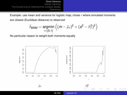
Example: use mean and variance for logistic map; chose r where simulated moments

are closest (Euclidean distance) to observed

rMSM = argminr∈[0,1]

((m − µr )

2 + (s2 − σ2r )2

)No particular reason to weight both moments equally

0.0 0.2 0.4 0.6 0.8 1.0

0.0

0.1

0.2

0.3

0.4

0.5

0.6

r

Mea

n of

X

0.0 0.2 0.4 0.6 0.8 1.0

0.00

0.02

0.04

0.06

0.08

0.10

0.12

r

Var

ianc

e of

X

bµr bσ2r

36-462 Lecture 19

Direct InferenceIndirect Inference

The Correct Line on Inference from Complex ModelsReferences

0.65 0.70 0.75 0.80 0.85 0.90 0.95

05

1015

2025

30

Density of simulated moment estimates

N = 500 Bandwidth = 0.00342

Den

sity

Distribution of brMSM , time series length 100, true r = 0.9

36-462 Lecture 19

Direct InferenceIndirect Inference

The Correct Line on Inference from Complex ModelsReferences

Kinks in the curve of the moments: potentially confusing tooptimizer, reduces sensitivitybig change in parameter leads to negligible change in moments

curve crossing itself ⇒ non-identifiability

0.0 0.1 0.2 0.3 0.4 0.5 0.6

0.00

0.02

0.04

0.06

0.08

0.10

0.12

mean

var

36-462 Lecture 19

Direct InferenceIndirect Inference

The Correct Line on Inference from Complex ModelsReferences

The Progress of Statistical Methods

First stage calculate likelihood, solve explicitly for MLESecond stage can’t solve for MLE but can still write down

likelihood, calculate it, and maximize numericallyThird stage even calculating the likelihood is intractable

Outstanding example: hidden or latent variables Y1,Y2, . . . plusobserved X1,X2, . . .

36-462 Lecture 19

Direct InferenceIndirect Inference

The Correct Line on Inference from Complex ModelsReferences

Why Finding the Likelihood Becomes Hard

Likelihood become an integral/sum over all possiblecombinations of latent variables compatible with observations:

Prθ (X n1 = xn

1 )

=

∫dyn

1 Prθ (X n1 = xn

1 ,Yn1 = yn

1 )

=

∫dyn

1 Prθ (Y n1 = yn

1 )n∏

i=1

Prθ

(Xi = xi |Y n

1 = yn1 ,X

i−11 = x i−1

1

)Evaluating this sum-over-histories is, itself, a hard problemOne approach: Expectation-Maximization algorithm, try tosimultaneously estimate latent variables and parameters (Nealand Hinton, 1998)Standard, clever, often messy

36-462 Lecture 19

Direct InferenceIndirect Inference

The Correct Line on Inference from Complex ModelsReferences

Indirect Inference

We have a model with parameter θ from which we can simulatealso: data yIntroduce an auxiliary model which is wrong but easy to fitFit auxiliary to data, get parameters βSimulate from model to produce yS

θ — different simulations fordifferent values of θFit auxiliary to simulations, get βS

θ

Pick θ such that βSθ is as close as possible to β

Improvement: do several simulation runs at each θ, average βSθ

over runs

36-462 Lecture 19

Direct InferenceIndirect Inference

The Correct Line on Inference from Complex ModelsReferences

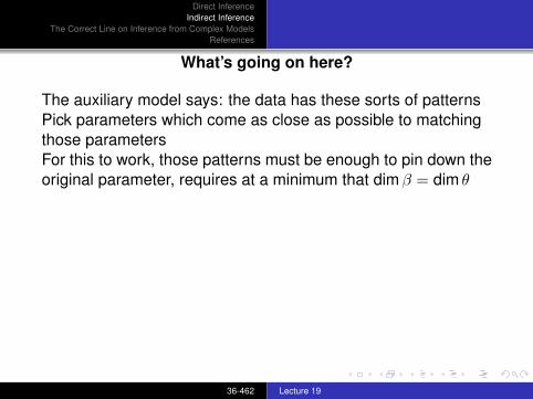
What’s going on here?

The auxiliary model says: the data has these sorts of patternsPick parameters which come as close as possible to matchingthose parametersFor this to work, those patterns must be enough to pin down theoriginal parameter, requires at a minimum that dimβ = dim θ

36-462 Lecture 19

Direct InferenceIndirect Inference

The Correct Line on Inference from Complex ModelsReferences

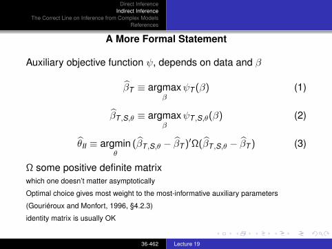
A More Formal Statement

Auxiliary objective function ψ, depends on data and β

βT ≡ argmaxβ

ψT (β) (1)

βT ,S,θ ≡ argmaxβ

ψT ,S,θ(β) (2)

θII ≡ argminθ

(βT ,S,θ − βT )′Ω(βT ,S,θ − βT ) (3)

Ω some positive definite matrixwhich one doesn’t matter asymptotically

Optimal choice gives most weight to the most-informative auxiliary parameters

(Gouriéroux and Monfort, 1996, §4.2.3)

identity matrix is usually OK

36-462 Lecture 19

Direct InferenceIndirect Inference

The Correct Line on Inference from Complex ModelsReferences

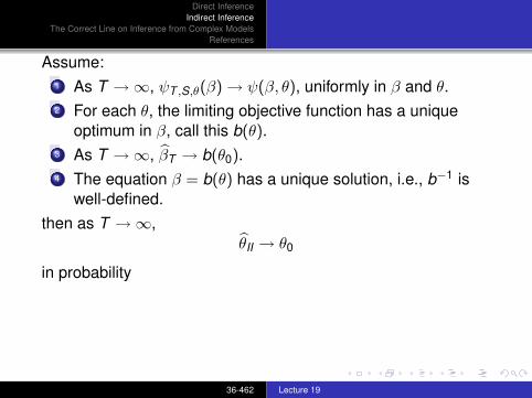
Assume:1 As T →∞, ψT ,S,θ(β) → ψ(β, θ), uniformly in β and θ.2 For each θ, the limiting objective function has a unique

optimum in β, call this b(θ).3 As T →∞, βT → b(θ0).4 The equation β = b(θ) has a unique solution, i.e., b−1 is

well-defined.then as T →∞,

θII → θ0

in probability

36-462 Lecture 19

Direct InferenceIndirect Inference

The Correct Line on Inference from Complex ModelsReferences

Asymptotic Distribution of Indirect Estimates

(Gouriéroux and Monfort, 1996, §4.2.3)

Under additional (long, technical) regularity conditions, θII − θ0 isasymptotically Gaussian with mean 0Variance ∝ 1

T

(1 + 1

S

)Variance depends on something like the Fisher informationmatrix, only with ∂b/∂θ in the role of ∂pθ/∂θbasically, how sensitive is the auxiliary parameter to shifts in the underlying true

parameter?

36-462 Lecture 19

Direct InferenceIndirect Inference

The Correct Line on Inference from Complex ModelsReferences

Checking Indirect Inference

Given real and auxiliary model, will indirect inference work, i.e.,be consistent?

Do the math Provides proof; often hard (because thesimulation model leads to difficulty-to-manipulatedistributions)

Simulate some more Simulate from model for a particular θ,apply II, check that estimates are getting closer toθ as simulation grows, repeat for multiple θNot as fool-proof but just requires time (you haveall the code already)

36-462 Lecture 19

Direct InferenceIndirect Inference

The Correct Line on Inference from Complex ModelsReferences

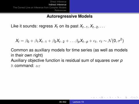
Autoregressive Models

Like it sounds: regress Xt on its past Xt−1,Xt−2, . . .

Xt = β0 + β1Xt−1 + β2Xt−2 + . . . βpXt−p + εt , εt ∼ N (0, σ2)

Common as auxiliary models for time series (as well as modelsin their own right)Auxiliary objective function is residual sum of squares over pR command: ar

36-462 Lecture 19

Direct InferenceIndirect Inference

The Correct Line on Inference from Complex ModelsReferences

Example: Logistic Map + Noise

Take logistic map and add Gaussian noise to each observation

xt = yt + εt , εt ∼ N (0, σ2)

yt+1 = 4ryt(1− yt)

Any sequence xT1 could be produced by any r

logistic.noisy.ts <- function(timelength,r,initial.cond=NULL,noise.sd=0.1)

x <- logistic.map.ts(timelength,r,initial.cond)return(x+rnorm(timelength,0,noise.sd))

Assume that σ2 is known — simplifies plotting if only oneunknown parameter! Set it to σ2 = 0.1

36-462 Lecture 19

Direct InferenceIndirect Inference

The Correct Line on Inference from Complex ModelsReferences

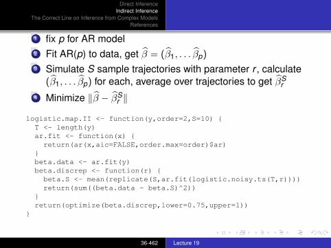
1 fix p for AR model2 Fit AR(p) to data, get β = (β1, . . . βp)

3 Simulate S sample trajectories with parameter r , calculate(β1, . . . βp) for each, average over trajectories to get βS

r

4 Minimize ‖β − βSr ‖

logistic.map.II <- function(y,order=2,S=10) T <- length(y)ar.fit <- function(x)

return(ar(x,aic=FALSE,order.max=order)$ar)beta.data <- ar.fit(y)beta.discrep <- function(r)

beta.S <- mean(replicate(S,ar.fit(logistic.noisy.ts(T,r))))return(sum((beta.data - beta.S)^2))

return(optimize(beta.discrep,lower=0.75,upper=1))

36-462 Lecture 19

Direct InferenceIndirect Inference

The Correct Line on Inference from Complex ModelsReferences

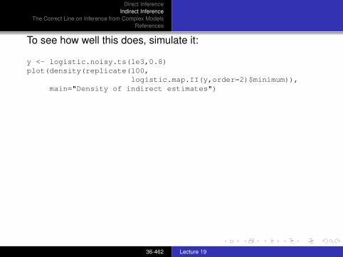
To see how well this does, simulate it:

y <- logistic.noisy.ts(1e3,0.8)plot(density(replicate(100,

logistic.map.II(y,order=2)$minimum)),main="Density of indirect estimates")

36-462 Lecture 19

Direct InferenceIndirect Inference

The Correct Line on Inference from Complex ModelsReferences

0.76 0.78 0.80 0.82 0.84 0.86 0.88

05

1015

20

Density of indirect estimates

N = 100 Bandwidth = 0.006528

Den

sity

Some bias (here upward) but it shrinks as T grows, and it’s pretty tight around the truevalue (r = 0.8)Notice: fixed data set, all variability is from simulation

Also: p = 2 is arbitrary, can use more simulation to pick good/best

36-462 Lecture 19

Direct InferenceIndirect Inference

The Correct Line on Inference from Complex ModelsReferences

r = 0.8 is periodic, what about chaos, say r = 0.9?

plot(density(replicate(30,logistic.map.II(logistic.noisy.ts(1e3,r=0.9),

order=2)$minimum)),main="Density of indirect estimates, r=0.9")

re-generate data each time

36-462 Lecture 19

Direct InferenceIndirect Inference

The Correct Line on Inference from Complex ModelsReferences

0.82 0.84 0.86 0.88 0.90 0.92

05

1015

2025

3035

Density of indirect estimates, r=0.9

N = 30 Bandwidth = 0.003931

Den

sity

36-462 Lecture 19

Direct InferenceIndirect Inference

The Correct Line on Inference from Complex ModelsReferences

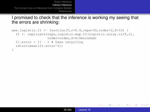
I promised to check that the inference is working my seeing thatthe errors are shrinking:

mse.logistic.II <- function(T,r=0.9,reps=30,order=2,S=10) II <- replicate(reps,logistic.map.II(logistic.noisy.ts(T,r),

order=order,S=S)$minimum)II.error = II - r # Uses recyclingreturn(mean(II.error^2))

36-462 Lecture 19

Direct InferenceIndirect Inference

The Correct Line on Inference from Complex ModelsReferences

500 1000 1500 2000

0.00

020.

0006

0.00

10

Mean squared error of indirect inference, r=0.9

T

MS

E

Black: mean squared error bθII , S = 10, average of 30 replications each of length T , all

with r = 0.9; blue: curve ∝ T−1, fitted through last data point

36-462 Lecture 19

Direct InferenceIndirect Inference

The Correct Line on Inference from Complex ModelsReferences

The Correct Line on Inference from Complex Models

MORE SCIENCE, FEWER F -TESTS

Craft a really good scientific modelrepresent your actual knowledge/assumptions/guesswork“it’s in my regression textbook” isn’t a scientific justificationmust be able to simulate it

Pick a reasonable auxiliary modelWorks on your observable dataEasy to fitPredicts well is nice but not necessary

Estimate parameters of complex model by indirectinferenceTest hypotheses by indirect inference as well (Gouriérouxet al., 1993; Kendall et al., 2005)

36-462 Lecture 19

Direct InferenceIndirect Inference

The Correct Line on Inference from Complex ModelsReferences

Gouriéroux, Christian and Alain Monfort (1996).Simulation-Based Econometric Methods. Oxford, England:Oxford University Pres.

Gouriéroux, Christian, Alain Monfort and E. Renault (1993).“Indirect Inference.” Journal of Applied Econometrics, 8:S85–S118. URL http://www.jstor.org/pss/2285076.

Kendall, Bruce E., Stephen P. Ellner, Edward Mccauley,Simon N. Wood, Cheryl J. Briggs, William W. Murdoch andPeter Turchin (2005). “Population Cycles in the Pine LooperMoth: Dynamical Tests of Mechanistic Hypotheses.”Ecological Monographs, 75: 259–276. URLhttp://www.eeb.cornell.edu/Ellner/pubs/CPDBupalusEcolMonog05.pdf.

Neal, Radford M. and Geoffrey E. Hinton (1998). “A View of theEM Algorithm that Justifies Incremental, Sparse, and OtherVariants.” In Learning in Graphical Models (Michael I. Jordan,

36-462 Lecture 19

Direct InferenceIndirect Inference

The Correct Line on Inference from Complex ModelsReferences

ed.), pp. 355–368. Dordrecht: Kluwer Academic. URLhttp://www.cs.toronto.edu/~radford/em.abstract.html.

Nevel’son, M. B. and R. Z. Has’minskii (1972/1976). StochasticApproximation and Recursive Estimation, vol. 47 ofTranslations of Mathematical Monographs. Providence,Rhode Island: American Mathematical Society. Translated bythe Israel Program for Scientific Translations and B. Silverfrom Stokhasticheskaia approksimatsia i rekurrentnoeotsenivanie, Moscow: Nauka.

Robbins, Herbert and Sutton Monro (1951). “A StochasticApproximation Method.” Annals of Mathematical Statistics,22: 400–407. URL http://projecteuclid.org/euclid.aoms/1177729586.

Smith, Jr., Anthony A. (forthcoming). “Indirect Inference.” InNew Palgrave Dictionary of Economics (Stephen Durlauf and

36-462 Lecture 19

Direct InferenceIndirect Inference

The Correct Line on Inference from Complex ModelsReferences

Lawrence Blume, eds.). London: Palgrave Macmillan, 2ndedn. URLhttp://www.econ.yale.edu/smith/palgrave7.pdf.

36-462 Lecture 19