(chapman & hall_crc pure and applied mathematics) apelian, christopher_ mathew, akhil_ surace,...
DESCRIPTION
variable complejaTRANSCRIPT


Real and Complex Analysis
C8067_FM.indd 1 11/3/09 1:42:10 PM

PURE AND APPLIED MATHEMATICS
A Program of Monographs, Textbooks, and Lecture Notes
EXECUTIVE EDITORS
EDITORIAL BOARD
Earl J. TaftRutgers University
Piscataway, New Jersey
Zuhair NashedUniversity of Central Florida
Orlando, Florida
M. S. BaouendiUniversity of California,
San Diego
Jane CroninRutgers University
Jack K. HaleGeorgia Institute of Technology
S. KobayashiUniversity of California,
Berkeley
Marvin MarcusUniversity of California,
Santa Barbara
W. S. MasseyYale University
Anil NerodeCornell University
Freddy van OystaeyenUniversity of Antwerp,Belgium
Donald PassmanUniversity of Wisconsin,Madison
Fred S. RobertsRutgers University
David L. RussellVirginia Polytechnic Instituteand State University
Walter SchemppUniversität Siegen
C8067_FM.indd 2 11/3/09 1:42:10 PM

MONOGRAPHS AND TEXTBOOKS INPURE AND APPLIED MATHEMATICS
Recent Titles
Christof Eck, Jiri Jarusek, and Miroslav Krbec, Unilateral Contact Problems: Variational Methods and Existence Theorems (2005)
M. M. Rao, Conditional Measures and Applications, Second Edition (2005)
A. B. Kharazishvili, Strange Functions in Real Analysis, Second Edition (2006)
Vincenzo Ancona and Bernard Gaveau, Differential Forms on Singular Varieties: De Rham and Hodge Theory Simpli!ed (2005)
Santiago Alves Tavares, Generation of Multivariate Hermite Interpolating Polynomials (2005)
Sergio Macías, Topics on Continua (2005)
Mircea Sofonea, Weimin Han, and Meir Shillor, Analysis and Approximation of Contact Problems with Adhesion or Damage (2006)
Marwan Moubachir and Jean-Paul Zolésio, Moving Shape Analysis and Control: Applications to Fluid Structure Interactions (2006)
Alfred Geroldinger and Franz Halter-Koch, Non-Unique Factorizations: Algebraic, Combinatorial and Analytic Theory (2006)
Kevin J. Hastings, Introduction to the Mathematics of Operations Research with Mathematica®, Second Edition (2006)
Robert Carlson, A Concrete Introduction to Real Analysis (2006)
John Dauns and Yiqiang Zhou, Classes of Modules (2006)
N. K. Govil, H. N. Mhaskar, Ram N. Mohapatra, Zuhair Nashed, and J. Szabados, Frontiers in Interpolation and Approximation (2006)
Luca Lorenzi and Marcello Bertoldi, Analytical Methods for Markov Semigroups (2006)
M. A. Al-Gwaiz and S. A. Elsanousi, Elements of Real Analysis (2006)
Theodore G. Faticoni, Direct Sum Decompositions of Torsion-Free Finite Rank Groups (2007)
R. Sivaramakrishnan, Certain Number-Theoretic Episodes in Algebra (2006)
Aderemi Kuku, Representation Theory and Higher Algebraic K-Theory (2006)
Robert Piziak and P. L. Odell, Matrix Theory: From Generalized Inverses to Jordan Form (2007)
Norman L. Johnson, Vikram Jha, and Mauro Biliotti, Handbook of Finite Translation Planes (2007)
Lieven Le Bruyn, Noncommutative Geometry and Cayley-smooth Orders (2008)
Fritz Schwarz, Algorithmic Lie Theory for Solving Ordinary Differential Equations (2008)
Jane Cronin, Ordinary Differential Equations: Introduction and Qualitative Theory, Third Edition (2008)
Su Gao, Invariant Descriptive Set Theory (2009)
Christopher Apelian and Steve Surace, Real and Complex Analysis (2010)
C8067_FM.indd 3 11/3/09 1:42:10 PM

C8067_FM.indd 4 11/3/09 1:42:10 PM

Real and Complex Analysis
Christopher ApelianSteve Suracewith Akhil Mathew
C8067_FM.indd 5 11/3/09 1:42:10 PM
Chapman & Hall/CRCTaylor & Francis Group6000 Broken Sound Parkway NW, Suite 300Boca Raton, FL 33487-2742
© 2010 by Taylor and Francis Group, LLCChapman & Hall/CRC is an imprint of Taylor & Francis Group, an Informa business
No claim to original U.S. Government works
Printed in the United States of America on acid-free paper10 9 8 7 6 5 4 3 2 1
International Standard Book Number-13: 978-1-58488-807-9 (Ebook-PDF)
This book contains information obtained from authentic and highly regarded sources. Reasonable efforts have been made to publish reliable data and information, but the author and publisher cannot assume responsibility for the validity of all materials or the consequences of their use. The authors and publishers have attempted to trace the copyright holders of all material reproduced in this publication and apologize to copyright holders if permission to publish in this form has not been obtained. If any copyright material has not been acknowledged please write and let us know so we may rectify in any future reprint.
Except as permitted under U.S. Copyright Law, no part of this book may be reprinted, reproduced, transmit-ted, or utilized in any form by any electronic, mechanical, or other means, now known or hereafter invented, including photocopying, microfilming, and recording, or in any information storage or retrieval system, without written permission from the publishers.
For permission to photocopy or use material electronically from this work, please access www.copyright.com (http://www.copyright.com/) or contact the Copyright Clearance Center, Inc. (CCC), 222 Rosewood Drive, Danvers, MA 01923, 978-750-8400. CCC is a not-for-profit organization that provides licenses and registration for a variety of users. For organizations that have been granted a photocopy license by the CCC, a separate system of payment has been arranged.
Trademark Notice: Product or corporate names may be trademarks or registered trademarks, and are used only for identification and explanation without intent to infringe.Visit the Taylor & Francis Web site athttp://www.taylorandfrancis.comand the CRC Press Web site athttp://www.crcpress.com

To my wife Paula.
For the sacrifices she made while this book was being written.
And to Ellie.For being exactly who she is.
- CA
To family and friends.
- SS


CONTENTS
Preface . . . . . . . . . . . . . . . . . . . . . . . . . . . xv
Acknowledgments. . . . . . . . . . . . . . . . . . . . . xvii
The Authors . . . . . . . . . . . . . . . . . . . . . . . . xix
1. The Spaces R, Rk, and C . . . . . . . . . . . . . . . . . 1
1 THE REAL NUMBERS R . . . . . . . . . . . . . . . . . . . . . . . 1
Properties of the Real Numbers R, 2. The Absolute Value, 7. Intervalsin R, 10
2 THE REAL SPACES Rk . . . . . . . . . . . . . . . . . . . . . . . . 10
Properties of the Real Spaces Rk, 11. Inner Products and Norms on
Rk, 14. Intervals in R
k, 18
3 THE COMPLEX NUMBERS C . . . . . . . . . . . . . . . . . . . . . 19
An Extension of R2, 19. Properties of Complex Numbers, 21. A
Norm on C and the Complex Conjugate of z, 24. Polar Notationand the Arguments of z, 26. Circles, Disks, Powers, and Roots, 30.Matrix Representation of Complex Numbers, 34
4 SUPPLEMENTARY EXERCISES . . . . . . . . . . . . . . . . . . . . 35
2. Point-Set Topology . . . . . . . . . . . . . . . . . . . . 41
1 BOUNDED SETS . . . . . . . . . . . . . . . . . . . . . . . . . . . 42
Bounded Sets in X, 42. Bounded Sets in R, 44. Spheres, Balls, andNeighborhoods, 47
2 CLASSIFICATION OF POINTS . . . . . . . . . . . . . . . . . . . . 50
Interior, Exterior, and Boundary Points, 50. Limit Points and Iso-lated Points, 53
3 OPEN AND CLOSED SETS . . . . . . . . . . . . . . . . . . . . . . 55
Open Sets, 55. Closed Sets, 58. Relatively Open and Closed Sets, 61.Density, 62
ix

x CONTENTS
4 NESTED INTERVALS AND THE BOLZANO-WEIERSTRASS THEOREM 63
Nested Intervals, 63. The Bolzano-Weierstrass Theorem, 66
5 COMPACTNESS AND CONNECTEDNESS . . . . . . . . . . . . . . 69
Compact Sets, 69. The Heine-Borel Theorem, 71. Connected Sets, 72
6 SUPPLEMENTARY EXERCISES . . . . . . . . . . . . . . . . . . . . 75
3. Limits and Convergence . . . . . . . . . . . . . . . . . 83
1 DEFINITIONS AND FIRST PROPERTIES . . . . . . . . . . . . . . . 84
Definitions and Examples, 84. First Properties of Sequences, 89
2 CONVERGENCE RESULTS FOR SEQUENCES . . . . . . . . . . . . . 90
General Results for Sequences in X, 90. Special Results for Sequencesin R and C, 92
3 TOPOLOGICAL RESULTS FOR SEQUENCES . . . . . . . . . . . . . 97
Subsequences in X, 97. The Limit Superior and Limit Inferior, 100.Cauchy Sequences and Completeness, 104
4 PROPERTIES OF INFINITE SERIES . . . . . . . . . . . . . . . . . . 108
Definition and Examples of Series in X, 108. Basic Results for Seriesin X, 110. Special Series, 115. Testing for Absolute Convergence inX, 120
5 MANIPULATIONS OF SERIES IN R . . . . . . . . . . . . . . . . . . 123
Rearrangements of Series, 123. Multiplication of Series, 125.Definition of ex for x ! R, 128
6 SUPPLEMENTARY EXERCISES . . . . . . . . . . . . . . . . . . . . 128
4. Functions: Definitions and Limits . . . . . . . . . . . . 135
1 DEFINITIONS . . . . . . . . . . . . . . . . . . . . . . . . . . . . . 135
Notation and Definitions, 136. Complex Functions, 137
2 FUNCTIONS AS MAPPINGS . . . . . . . . . . . . . . . . . . . . . 139
Images and Preimages, 139. Bounded Functions, 141. CombiningFunctions, 142. One-to-One Functions and Onto Functions, 144.Inverse Functions, 147
3 SOME ELEMENTARY COMPLEX FUNCTIONS . . . . . . . . . . . . 148
Complex Polynomials and Rational Functions, 148. The ComplexSquare Root Function, 149. The Complex Exponential Function, 150.The Complex Logarithm, 151. Complex Trigonometric Functions, 154
4 LIMITS OF FUNCTIONS . . . . . . . . . . . . . . . . . . . . . . . 156
Definition and Examples, 156. Properties of Limits of Functions, 160.Algebraic Results for Limits of Functions, 163
5 SUPPLEMENTARY EXERCISES . . . . . . . . . . . . . . . . . . . . 171

CONTENTS xi
5. Functions: Continuity and Convergence . . . . . . . . . 177
1 CONTINUITY . . . . . . . . . . . . . . . . . . . . . . . . . . . . . 177
Definitions, 177. Examples of Continuity, 179. Algebraic Proper-ties of Continuous Functions, 184. Topological Properties andCharacterizations, 187. Real Continuous Functions, 191
2 UNIFORM CONTINUITY . . . . . . . . . . . . . . . . . . . . . . . 198
Definition and Examples, 198. Topological Properties andConsequences, 201. Continuous Extensions, 203
3 SEQUENCES AND SERIES OF FUNCTIONS . . . . . . . . . . . . . . 208
Definitions and Examples, 208. Uniform Convergence, 210. Seriesof Functions, 216. The Tietze Extension Theorem, 219
4 SUPPLEMENTARY EXERCISES . . . . . . . . . . . . . . . . . . . . 222
6. The Derivative . . . . . . . . . . . . . . . . . . . . . . 233
1 THE DERIVATIVE FOR f : D1! R . . . . . . . . . . . . . . . . . 234
Three Definitions Are Better Than One, 234. First Properties andExamples, 238. Local Extrema Results and the Mean ValueTheorem, 247. Taylor Polynomials, 250. Differentiation of Sequencesand Series of Functions, 255
2 THE DERIVATIVE FOR f : Dk! R . . . . . . . . . . . . . . . . . 257
Definition, 258. Partial Derivatives, 260. The Gradient and Direc-tional Derivatives, 262. Higher-Order Partial Derivatives, 266.Geometric Interpretation of Partial Derivatives, 268. Some UsefulResults, 269
3 THE DERIVATIVE FOR f : Dk! Rp . . . . . . . . . . . . . . . . . 273
Definition, 273. Some Useful Results, 283. DifferentiabilityClasses, 289
4 THE DERIVATIVE FOR f : D ! C . . . . . . . . . . . . . . . . . . 291
Three Derivative Definitions Again, 292. Some Useful Results, 295.The Cauchy-Riemann Equations, 297. The z and z Derivatives, 305
5 THE INVERSE AND IMPLICIT FUNCTION THEOREMS . . . . . . . 309
Some Technical Necessities, 310. The Inverse Function Theorem, 313.The Implicit Function Theorem, 318
6 SUPPLEMENTARY EXERCISES . . . . . . . . . . . . . . . . . . . . 321
7. Real Integration . . . . . . . . . . . . . . . . . . . . . . 335
1 THE INTEGRAL OF f : [a, b] ! R . . . . . . . . . . . . . . . . . . 335
Definition of the Riemann Integral, 335. Upper and Lower Sumsand Integrals, 339. Relating Upper and Lower Integrals toIntegrals, 346

xii CONTENTS
2 PROPERTIES OF THE RIEMANN INTEGRAL . . . . . . . . . . . . . 349
Classes of Bounded Integrable Functions, 349. Elementary Proper-ties of Integrals, 354. The Fundamental Theorem of Calculus, 360
3 FURTHER DEVELOPMENT OF INTEGRATION THEORY . . . . . . . 363
Improper Integrals of Bounded Functions, 363. Recognizing a Se-quence as a Riemann Sum, 366. Change of Variables Theorem, 366.Uniform Convergence and Integration, 367
4 VECTOR-VALUED AND LINE INTEGRALS. . . . . . . . . . . . . . 369
The Integral of f : [a, b] ! Rp, 369. Curves and Contours, 372.
Line Integrals, 377
5 SUPPLEMENTARY EXERCISES . . . . . . . . . . . . . . . . . . . . 381
8. Complex Integration . . . . . . . . . . . . . . . . . . . 387
1 INTRODUCTION TO COMPLEX INTEGRALS . . . . . . . . . . . . . 387
Integration over an Interval, 387. Curves and Contours, 390.Complex Line Integrals, 393
2 FURTHER DEVELOPMENT OF COMPLEX LINE INTEGRALS . . . . 400
The Triangle Lemma, 400. Winding Numbers, 404. Antiderivativesand Path-Independence, 408. Integration in Star-Shaped Sets, 410
3 CAUCHY’S INTEGRAL THEOREM AND ITS CONSEQUENCES . . . 415
Auxiliary Results, 416. Cauchy’s Integral Theorem, 420.Deformation of Contours, 423
4 CAUCHY’S INTEGRAL FORMULA . . . . . . . . . . . . . . . . . . 428
The Various Forms of Cauchy’s Integral Formula, 428. The Maxi-mum Modulus Theorem, 433. Cauchy’s Integral Formula for Higher-Order Derivatives, 435
5 FURTHER PROPERTIES OF COMPLEX DIFFERENTIABLE FUNCTIONS 438
Harmonic Functions, 438. A Limit Result, 439.Morera’s Theorem, 440. Liouville’s Theorem, 441. The Fundamen-tal Theorem of Algebra, 442
6 APPENDICES: WINDING NUMBERS REVISITED . . . . . . . . . . 443
A Geometric Interpretation, 443. Winding Numbers of Simple ClosedContours, 447
7 SUPPLEMENTARY EXERCISES . . . . . . . . . . . . . . . . . . . . 450
9. Taylor Series, Laurent Series, and the Residue Calculus 455
1 POWER SERIES . . . . . . . . . . . . . . . . . . . . . . . . . . . . 456
Definition, Properties, and Examples, 456. Manipulations of PowerSeries, 464
2 TAYLOR SERIES . . . . . . . . . . . . . . . . . . . . . . . . . . . 473
CONTENTS xiii
3 ANALYTIC FUNCTIONS . . . . . . . . . . . . . . . . . . . . . . . 481
Definition and Basic Properties, 481. Complex AnalyticFunctions, 483
4 LAURENT’S THEOREM FOR COMPLEX FUNCTIONS . . . . . . . . 4875 SINGULARITIES . . . . . . . . . . . . . . . . . . . . . . . . . . . 493
Definitions, 493. Properties of Functions Near Singularities, 496
6 THE RESIDUE CALCULUS . . . . . . . . . . . . . . . . . . . . . . 502
Residues and the Residue Theorem, 502. Applications to Real Im-proper Integrals, 507
7 SUPPLEMENTARY EXERCISES . . . . . . . . . . . . . . . . . . . . 512
10. Complex Functions as Mappings . . . . . . . . . . . . . 5151 THE EXTENDED COMPLEX PLANE . . . . . . . . . . . . . . . . . 5152 LINEAR FRACTIONAL TRANSFORMATIONS . . . . . . . . . . . . 519
Basic LFTs, 519. General LFTs, 521
3 CONFORMAL MAPPINGS . . . . . . . . . . . . . . . . . . . . . . 524
Motivation and Definition, 524. More Examples of ConformalMappings, 527. The Schwarz Lemma and the Riemann MappingTheorem, 530
4 SUPPLEMENTARY EXERCISES . . . . . . . . . . . . . . . . . . . . 534
Bibliography. . . . . . . . . . . . . . . . . . . . . . . . 537
Index . . . . . . . . . . . . . . . . . . . . . . . . . . . . 539


PREFACE
The last thing one knows when writing a book is what to put first.
Blaise Pascal
This is a text for a two-semester course in analysis at the advanced under-graduate or first-year graduate level, especially suited for liberal arts col-leges. Analysis is a very old and established subject. While virtually none ofthe content of this work is original to the authors, we believe its organizationand presentation are unique. Unlike other undergraduate level texts of whichwe are aware, this one develops both the real and complex theory together.Our exposition thus allows for a unified and, we believe, more elegant pre-sentation of the subject. It is also consistent with the recommendations givenin the Mathematical Association of America’s 2004 Curriculum Guide, avail-able online at www.maa.org/cupm.
We believe that learning real and complex analysis separately can lead stu-dents to compartmentalize the two subjects, even though they—like all ofmathematics—are inextricably interconnected. Learning them together showsthe connections at the outset. The approach has another advantage. In smalldepartments (such as ours), a combined development allows for a more stream-lined sequence of courses in real and complex function theory (in particular,a two-course sequence instead of the usual three), a consideration that moti-vated Drew University to integrate real and complex analysis several yearsago. Since then, our yearly frustration of having to rely on two separate texts,one for real function theory and one for complex function theory, ultimatelyled us to begin writing a text of our own.
We wrote this book with the student in mind. While we assume the stan-dard background of a typical junior or senior undergraduate mathematicsmajor or minor at today’s typical American university, the book is largelyself-contained. In particular, the reader should know multivariable calculusand the basic notions of set theory and logic as presented in a “gateway”course for mathematics majors or minors. While we will make use of matri-ces, knowledge of linear algebra is helpful, but not necessary.
We have also included over 1,000 exercises. The reader is encouraged to doall of the embedded exercises that occur within the text, many of which are
xv
xvi PREFACE
necessary to understand the material or to complete the development of aparticular topic. To gain a stronger understanding of the subject, however,the serious student should also tackle some of the supplementary exercisesat the end of each chapter. The supplementary exercises include both routineskills problems as well as more advanced problems that lead the reader tonew results not included in the text proper.
Both students and instructors will find this book’s website, http://users.drew.edu/capelian/rcanalysis.html, helpful. Partial solutions orhints to selected exercises, supplementary materials and problems, and rec-ommendations for further reading will appear there. Questions or commentscan be sent either to [email protected], or to [email protected].
This text was typeset using LaTeX! 2! and version 5.5 of the WinEdt! edit-ing environment. All figures were created with Adobe Illustrator!. The math-ematical computing package Mathematica! was also used in the creationof Figures 6.1, 8.2, 8.19, 8.22, 10.1, 10.10, and 10.13. The quotes that openeach chapter are from the Mathematical Quotation Server, at http://math.furman.edu/~mwoodard/mqs/mquot.shtml.
We sincerely hope this book will help make your study of analysis a reward-ing experience.
CASS

ACKNOWLEDGMENTS
Everything of importance has been said before by somebody who did not discover it.
Alfred North Whitehead
We are indebted to many people for helping us produce this work, not leastof whom are those authors who taught us through their texts, including Drs.Fulks, Rudin, Churchill, Bartle, and many others listed in the bibliography.We also thank and credit our instructors at Rutgers University, New YorkUniversity, and the Courant Institute, whose lectures have inspired manyexamples, exercises, and insights. Our appreciation of analysis, its precision,power, and structure, was developed and nurtured by all of them. We are for-ever grateful to them for instilling in us a sense of its challenges, importance,and beauty. We would also like to thank our colleagues at Drew University,and our students, who provided such valuable feedback during the severalyears when drafts of this work were used to teach our course sequence of realand complex analysis. Most of all, we would like to extend our heartfelt grat-itude to Akhil Mathew, whose invaluable help has undoubtedly made this abetter book. Of course, we take full responsibility for any errors that mightyet remain. Finally, we thank our families. Without their unlimited support,this work would not have been possible.
xvii


THE AUTHORS
Christopher Apelian completed a Ph.D. in mathematics in 1993 at New YorkUniversity’s Courant Institute of Mathematical Sciences and then joined theDepartment of Mathematics and Computer Science at Drew University. Hehas published papers in the applications of probability and stochastic pro-cesses to the modeling of turbulent transport. His other interests include thefoundations and philosophy of mathematics and physics.
Steve Surace joined Drew University’s Department of Mathematics and Com-puter Science in 1987 after earning his Ph.D. in mathematics from New YorkUniversity’s Courant Institute. His mathematical interests include analysis,mathematical physics and cosmology. He is also the Associate Director ofthe New Jersey Governor’s School in the Sciences held at Drew Universityevery summer.
xix


1THE SPACES R, Rk
, AND C
We used to think that if we knew one, we knew two, because one and one are two.We are finding that we must learn a great deal more about “and.”
Sir Arthur Eddington
We begin our study of analysis with a description of those number systemsand spaces in which all of our subsequent work will be done. The real spacesR and Rk for k ! 2, and the complex number system C, are all vector spacesand have many properties in common.1 Among the real spaces, since eachspace Rk is actually a Cartesian product of k copies of R, such similaritiesare not surprising. It might seem worthwhile then to consider the real spacestogether, leaving the space C as the only special case. However, the set of realnumbers R and the set of complex numbers C both distinguish themselvesfrom the other real spaces Rk in a significant way: R and C are both fields.The space R is further distinguished in that it is an ordered field. For this rea-son, the real numbers R and the complex numbers C each deserve specialattention. We begin by formalizing the properties of the real numbers R. Wethen describe the higher-dimensional real spaces Rk . Finally, we introducethe rich and beautiful complex number system C.
1 THE REAL NUMBERS R
In a course on the foundations of mathematics, or even a transition coursefrom introductory to upper-level mathematics, one might have seen the de-velopment of number systems. Typically, such developments begin with thenatural numbers N = {1, 2, 3, . . .} and progress constructively to the realnumbers R. The first step in this progression is to supplement the natu-ral numbers with an additive identity, 0, and each natural number’s addi-tive inverse to arrive at the integers Z = {. . . ,"2,"1, 0, 1, 2, . . .} . One then
1Throughout our development Rk will be our concise designation for the higher-dimensional real spaces, i.e., k ! 2.
1

2 THE SPACES R, Rk, AND C
considers ratios of integers, thereby obtaining the rational number system
Q =!
pq : p, q # Z, q $= 0
". The real number system is then shown to include
Q as well as elements not in Q, the so-called irrational numbers I. That is,R = Q % I, where Q & I = !. In fact, N ' Z ' Q ' R. While it is reasonable,and even instructive, to “build up” the real number system from the sim-pler number systems in this way, this approach has its difficulties. For conve-nience, therefore, we choose instead to assume complete familiarity with thereal number system R, as well as its geometric interpretation as an infiniteline of points. Our purpose in this section is to describe the main proper-ties of R. This summary serves as a valuable review, but it also allows us tohighlight certain features of R that are typically left unexplored in previousmathematics courses.
1.1 Properties of the Real Numbers R
The Field Properties
The set of real numbers R consists of elements that can be combined accord-ing to two binary operations: addition and multiplication. These operations aretypically denoted by the symbols + and ·, respectively, so that given any twoelements x and y of R, their sum is denoted by x + y, and their product isdenoted by x · y, or more commonly, by xy (the · is usually omitted). Boththe sum and the product are themselves elements of R. Owing to this fact,we say that R is closed under addition and multiplication. The following al-gebraic properties of the real numbers are also known as the field properties,since it is exactly these properties that define a field as typically described ina course in abstract algebra.
1. (Addition is commutative) x + y = y + x for all x, y # R.
2. (Addition is associative) (x + y) + z = x + (y + z) for all x, y, z # R.
3. (Additive identity) There exists a unique element, denoted by 0 # R, suchthat x + 0 = x for all x # R.
4. (Additive inverse) For each x # R, there exists a unique element "x # R
such that x + ("x) = 0.
5. (Multiplication is commutative) xy = yx for all x, y # R.
6. (Multiplication is associative) (xy)z = x(yz) for all x, y, z # R.
7. (Multiplicative identity) There exists a unique element, denoted by 1 # R,such that 1x = x for all x # R.
8. (Multiplicative inverse) For each nonzero x # R, there exists a uniqueelement x"1
# R satisfying xx"1 = 1.
9. (Distributive property) x(y + z) = xy + xz for all x, y, z # R.
With the above properties of addition and multiplication, and the notionsof additive and multiplicative inverse as illustrated in properties 4 and 8,

THE REAL NUMBERS R 3
we can easily define the familiar operations of subtraction and division. Inparticular, subtraction of two real numbers, a and b, is denoted by the rela-tion a " b, and is given by a " b = a + ("b). Similarly, division of two realnumbers a and b is denoted by the relation a/b where it is necessary thatb $= 0, and is given by a/b = ab"1. The notions of subtraction and divisionare conveniences only, and are not necessary for a complete theory of the realnumbers.
The Order Properties
In an intuitive, geometric sense, the order properties of R are simply a preciseway of expressing when one real number lies to the left (or right) of anotheron the real line. More formally, an ordering on a set S is a relation, genericallydenoted by (, between any two elements of the set satisfying the followingtwo rules:
1. For any x, y # S, exactly one of the following holds: x ( y, x = y, y ( x.
2. For any x, y, z # S, x ( y and y ( z ) x ( z.
If the set S is also a field, as R is, the ordering might also satisfy two moreproperties:
3. For any x, y, z # S, x ( y ) x + z ( y + z.
4. If x, y # S are such that 0 ( x and 0 ( y, then 0 ( xy.
In the case where all four of the above properties are satisfied, S is called anordered field.
With any ordering ( on S, it is convenient to define the relation * accordingto the following convention. For x and y in S, we write y * x if and only ifx ( y.
For students of calculus, the most familiar ordering on R is the notion of“less than” denoted by <. Because the ordering < on R satisfies properties1 through 4 above, we refer to R as an ordered field. As we will soon see, notevery field with an ordering is an ordered field. That is, there are fields withorderings that do not satisfy properties 3 and 4.
The following list of facts summarizes some other useful order properties of< on R, each of which can be proved using properties 1 through 4 above.Suppose x, y, z, and w are real numbers. Then,
a) x < y if and only if 0 < y " x.
b) If x < y and w < z, then x + w < y + z.
c) If 0 < x and 0 < y, then 0 < x + y.
d) If 0 < z and x < y, then xz < yz.
e) If z < 0 and x < y, then yz < xz.

4 THE SPACES R, Rk, AND C
f) If 0 < x then 0 < x"1.
g) If x $= 0 then 0 < x2.
h) If x < y, then x < (x+y)2 < y.
! 1.1 Prove properties a) through h) using order properties 1 through 4 and the fieldproperties.
As in the general case described above, it is convenient to define the relation> on R according to the following rule. For x and y in R we will write y > xif and only if x < y. Students will recognize > as the “greater than” orderingon R. Note also that when a real number x satisfies 0 < x or x = 0, wewill write 0 + x and may refer to x as nonnegative. Similarly, when x satisfiesx < 0 or x = 0, we will write x + 0 and may refer to x as nonpositive. Ingeneral, we write x + y if either x < y or x = y. We may also write y ! xwhen x + y. These notations will be convenient in what follows.
! 1.2 A maximal element or maximum of a set A ! R is an element x " A suchthat a # x for all a " A. Likewise, a minimal element or minimum of a set A isan element y " A such that y # a for all a " A. When they exist, we will denote amaximal element of a set A by max A, and a minimal element of a set A by min A.Can you see why a set A ! R need not have a maximal or minimal element? If eithera maximal or a minimal element exists for A ! R, show that it is unique.
The Dedekind Completeness Property
Of all the properties of real numbers with which calculus students work, thecompleteness property is probably the one most taken for granted. In certainways it is also the most challenging to formalize. After being introduced tothe set Q, one might have initially thought that it comprised the whole realline. After all, between any two rational numbers there are infinitely manyother rational numbers (to see this, examine fact (viii) from the above listof properties carefully). However, as you have probably already discovered,,
2 is a real number that isn’t rational, and so the elements in Q, when linedup along the real line, don’t fill it up entirely. The irrational numbers “com-plete” the rational numbers by filling in these gaps in the real line. As simpleand straightforward as this sounds, we must make this idea more mathe-matically precise. What we will refer to as the Dedekind completeness propertyaccomplishes this. We state this property below.
The Dedekind Completeness Property Suppose A and B are nonempty sub-sets of R satisfying the following:
(i) R = A % B,
(ii) a < b for every a # A and every b # B.
Then either there exists a maximal element of A, or there exists a minimal element ofB.
THE REAL NUMBERS R 5
This characterization of the completeness property of R is related to what isknown more formally as a Dedekind cut.2 Because of (ii) and the fact that thesets A and B referred to in the Dedekind completeness property form a partitionof R (see the exercise below), we will sometimes refer to A and B as an orderedpartition of R. It can be shown that such an ordered partition of R uniquelydefines (or is uniquely defined by) a single real number x, which serves asthe dividing point between the subsets A and B. With respect to this divid-ing point x, the Dedekind completeness property of R is equivalent to thestatement that x satisfies the following: a + x + b for all a # A and for allb # B, and x belongs to exactly one of the sets A or B.
! 1.3 A partition of a set S is a collection of nonempty subsets {A!} of S satisfying#A! = S and A! $ A" = ! for ! %= ". Prove that any two sets A, B ! R satisfying
the Dedekind completeness property also form a partition of R.
We illustrate the Dedekind completeness property in the following example.
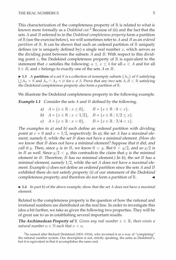
Example 1.1 Consider the sets A and B defined by the following.
a) A = {x # R : x + 0}, B = {x # R : 0 < x}.
b) A = {x # R : x < 1/2}, B = {x # R : 1/2 + x}.
c) A = {x # R : x < 0}, B = {x # R : 3/4 < x}.
The examples in a) and b) each define an ordered partition with dividingpoint at x = 0 and x = 1/2, respectively. In a), the set A has a maximal ele-ment, namely 0, while the set B does not have a minimal element. (How dowe know that B does not have a minimal element? Suppose that it did, andcall it y. Then, since y is in B, we know 0 < y. But 0 < y/2, and so y/2 isin B as well. Since y/2 < y, this contradicts the claim that y is the minimalelement in B. Therefore, B has no minimal element.) In b), the set B has aminimal element, namely 1/2, while the set A does not have a maximal ele-ment. Example c) does not define an ordered partition since the sets A and Bexhibited there do not satisfy property (i) of our statement of the Dedekindcompleteness property, and therefore do not form a partition of R. "
! 1.4 In part b) of the above example, show that the set A does not have a maximalelement.
Related to the completeness property is the question of how the rational andirrational numbers are distributed on the real line. In order to investigate thisidea a bit further, we take as given the following two properties. They will beof great use to us in establishing several important results.
The Archimedean Property of R Given any real number x # R, there exists anatural number n # N such that x < n.
2So named after Richard Dedekind (1831–1916), who invented it as a way of “completing”the rational number system. Our description is not, strictly speaking, the same as Dedekind’s,but it is equivalent in that it accomplishes the same end.

6 THE SPACES R, Rk, AND C
The Well-Ordered Property of N If S is a nonempty subset of N, then S has aminimal element.
The meaning of each of these properties is rather subtle. On first blush, itseems that the Archimedean property is making the uncontroversial claimthat there is no largest natural number. In fact, it is claiming a very signifi-cant characteristic of the real numbers, namely, that each real number is finite.When turned on its head, it also implies that there are no nonzero “infinites-imal” real numbers.3 The meaning of the well-ordered property of N is alsodeep. In fact, although we do not prove it here, it is equivalent to the principleof mathematical induction.
! 1.5 Establish the following:
a) Show that, for any positive real number x, there exists a natural number n suchthat 0 <
1n
< x. This shows that there are rational numbers arbitrarily close tozero on the real line. It also shows that there are real numbers between 0 and x.
b) Show that, for any real numbers x, y with x positive, there exists a natural numbern such that y < nx.
! 1.6 Use the Archimedean property and the well-ordered property to show that,for any real number x, there exists an integer n such that n & 1 # x < n. To do this,consider the following cases in order: x " Z, {x " R : x > 1}, {x " R : x ' 0}, {x "R : x < 0}.
We will now use the results of the previous exercises to establish an impor-tant property of the real line. We will show that between any two real num-bers there is a rational number. More specifically, we will show that for anytwo real numbers x and y satisfying x < y, there exists a rational number qsuch that x < q < y. To establish this, we will find m # N and n # Z suchthat mx < n < my. In a geometric sense, the effect of multiplying x and y bym is to “magnify” the space between x and y on the real line to ensure that itcontains an integer value, n. To begin the proof, note that 0 < y"x, and so bythe Archimedean property there exists m # N such that 0 < 1
m < y " x. Thisin turn implies that 1 < my " mx, or 1 + mx < my. According to a previousexercise, there exists an integer n such that n" 1 + mx < n. The right side ofthis double inequality is the desired mx < n. Adding 1 to the left side of thisdouble inequality obtains n + 1 + mx. But we have already established that1 + mx < my, so we have the desired n < my. Overall, we have shown thatthere exists m # N and n # Z such that mx < n < my. Dividing by m yieldsx < n/m < y, and the result is proved.
Not only have we shown that between any two real numbers there is a ratio-nal number, it is not hard to see how our result actually implies there are in-
3Loosely speaking, if ! and x are positive real numbers such that ! < x, the number ! iscalled infinitesimal if it satisfies n ! < x for all n # N. Sets with such infinitesimal elements arecalled non-Archimedean and are not a part of modern standard analysis. This is so despite theerroneous use of this term and a version of its associated concept among some mathematiciansduring the early days of analysis.

THE REAL NUMBERS R 7
finitely many rational numbers between any two real numbers. It also provesthat there was nothing special about zero two exercises ago. That is, there arerational numbers arbitrarily close to any real number.
! 1.7 Show that if # is irrational and q %= 0 is rational, then q# is irrational.
! 1.8 In this exercise, we will show that for any two real numbers x and y satisfyingx < y, there exists an irrational number # satisfying x < # < y. The result of this ex-ercise implies that there are infinitely many irrational numbers between any two realnumbers, and that there are irrational numbers arbitrarily close to any real number.To begin, consider the case 0 < x < y, and make use of the previous exercise.
1.2 The Absolute Value
We have seen several properties of real numbers, including algebraic prop-erties, order properties, and the completeness property, that give us a fullerunderstanding of what the real numbers are. To understand R even better, wewill need a tool that allows us to measure the magnitude of any real number.This task is accomplished by the familiar absolute value.
Definition 1.2 For any x # R, the absolute value of x is the nonnegativereal number denoted by |x| and defined by
|x| =
$"x for x < 0
x for x ! 0.
It is worth noting that for any pair of real numbers x and y, the differencex " y is also a real number, so we may consider the magnitude |x " y|. Ge-ometrically, |x| can be interpreted as the “distance” from the point x to theorigin, and similarly, |x " y| can be interpreted as the “distance” from thepoint x to the point y. The idea of distance between two points in a space isan important concept in analysis, and the geometric intuition it affords willbe exploited throughout what follows. The important role played by the ab-solute value in R as a way to quantify magnitudes and distances betweenpoints will be extended to Rk and C in the next chapter.
Note that a convenient, equivalent formula for computing the absolute value
of a real number x is given by |x| =,
x2. To see the equivalence, considerthe two cases x ! 0 and x < 0 separately. If x ! 0, then according to our
definition, |x| = x. Also,,
x2 = x, and so |x| =,
x2 for x ! 0. If x < 0,then our definition yields |x| = "x, while
,
x2 =%
("x)2 = "x. Therefore,
|x| =,
x2 for x < 0. This means for computing |x| is particularly useful inproving many of the following properties of the absolute value, which westate as a proposition.

8 THE SPACES R, Rk, AND C
Proposition 1.3 Absolute Value Properties
a) |x| ! 0 for all x # R, with equality if and only if x = 0.
b) |" x | = |x| for all x # R.
c) |x " y| = |y " x| for all x, y # R.
d) |x y| = |x| |y| for all x, y # R.
e)&&&xy
&&& = |x||y| for all x, y # R such that y $= 0.
f) If c ! 0, then |x| + c if and only if " c + x + c.
g) "|x| + x + |x| for all x # R.
PROOF
a) Clearly |x| =,
x2! 0 for all x # R. Note that |x| = 0 if and only if
,
x2 = 0 if and only if x2 = 0 if and only if x = 0.
b) |" x | =%
("x)2 =,
x2 = |x| for all x # R.
c) For all x, y # R, we have that |x " y| = |"(x " y)| by part b), and
|"(x " y)| = |y " x|.
d) For all x, y # R, we have |xy| =%
(x y)2 =%
x2 y2 =,
x2%
y2 = |x| |y|.
e)&&&xy
&&& =
'(xy
)2=*
x2
y2 =$
x2,
y2= |x|
|y| .
f) Note that
{x # R : |x| + c} = {x # R : |x| + c} & ({x # R : x ! 0} % {x # R : x < 0})
= {x # R : x ! 0, |x| + c} % {x # R : x < 0, |x| + c}
= {x # R : x ! 0, x + c} % {x # R : x < 0,"x + c}
= {x # R : 0 + x + c} % {x # R : "c + x < 0}
= {x # R : "c + x + c}.
g) We consider the proof casewise. If x ! 0, then "|x| + 0 + x = |x| + |x|.
If x < 0, then "|x| + "|x| = x < 0 + |x|. #
! 1.9 Show that if c > 0, then |x| < c if and only if &c < x < c.
The following corollary to the previous result is especially useful. It can serveas a convenient way to prove that a real number is, in fact, zero.
Corollary 1.4 Suppose x # R satisfies |x| < ! for all ! > 0. Then x = 0.

THE REAL NUMBERS R 9
! 1.10 Prove the above corollary. Show also that the conclusion still holds when thecondition |x| < $ is replaced by |x| # $.
! 1.11 If x < $ for every $ > 0, what can you conclude about x? Prove your claim.(Answer: x # 0.)
The inequalities in the following theorem are so important that they are worthstating separately from Proposition 1.3.
Theorem 1.5
a) |x ± y| + |x| + |y| for all x, y # R. The triangle inequality
b)&&|x|" |y|
&&+ |x ± y| for all x, y # R. The reverse triangle inequality
The results of the above theorem are sometimes stated together as&&|x|" |y|
&&+ |x ± y| + |x| + |y| for all x, y # R.
PROOF We prove the “+" case of the stated “±," in both a) and b), leavingthe “"" case to the reader. First, we establish |x + y| + |x| + |y|. We prove thiscasewise.
Case 1: If x + y ! 0, then |x + y| = x + y + |x| + |y| .
Case 2: If x + y < 0, then |x + y| = "(x + y) = "x " y + |x| + |y|.
Now we establish that&&|x|" |y|
&&+ |x + y| . Note by part a) that
|x| = |x + y " y| + |x + y| + |y| ,
which upon rearrangement gives |x|" |y| + |x + y| . Similarly, we have that
|y| = |y + x " x| + |y + x| + |x| = |x + y| + |x| ,
and so |x|" |y| ! " |x + y|. These results stated together yield
" |x + y| + |x|" |y| + |x + y| .
Finally, part f) of Proposition 1.3 gives&& |x|" |y|
&& + |x + y| . #
! 1.12 Finish the proof of the triangle inequality. That is, show that&& |x|& |y|
&& # |x & y| # |x| + |y| for all x, y " R.
! 1.13 Show that |x & z| # |x & y| + |y & z| for all x, y, and z " R.
A natural extension of the triangle inequality to a sum of n terms is oftenuseful.
Corollary 1.6 For all n # N and for all x1, x2, . . . , xn # R,
|x1 + x2 + x3 + · · · + xn| + |x1| + |x2| + |x3| + · · · + |xn|.
! 1.14 Prove the above corollary.

10 THE SPACES R, Rk, AND C
1.3 Intervals in R
To close out our discussion of the basic properties of the real numbers, weremind the reader of an especially convenient type of subset of R, and onethat will be extremely useful to us in our further development of analysis.Recall that an interval I ' R is the set of all real numbers lying between twospecified real numbers a and b where a < b. The numbers a and b are calledthe endpoints of the interval I . There are three types of intervals in R:
1. Closed. Both endpoints are included in the interval, in which case wedenote the interval as I = [a, b ].
2. Open. Both endpoints are excluded from the interval, in which case wedenote the interval as I = (a, b).
3. Half-Open or Half-Closed. Exactly one of the endpoints is excluded fromthe interval. If the excluded endpoint is a we write I = (a, b ]. If theexcluded endpoint is b we write I = [a, b).
In those cases where one wishes to denote an infinite interval we will makeuse of the symbols "- and -. For example, ("-, 0) represents the set ofnegative real numbers, also denoted by R", ("-, 2 ] represents all real num-bers less than or equal to 2, and (5,-) represents the set of real numbers thatare greater than 5. Note here that the symbols "- and - are not meant toindicate elements of the real number system; only that the collection of realnumbers being considered has no left or right endpoint, respectively. Because"- and - are not actually real numbers, they should never be consideredas included in the intervals in which they appear. For this reason, "- and- should always be accompanied by parentheses, not square brackets. Theopen interval (0, 1) is often referred to as the open unit interval, and the closedinterval [0, 1] as the closed unit interval. We will also have need to refer to thelength of an interval I ' R, a positive quantity we denote by " (I). If an inter-val I ' R has endpoints a < b # R, we define the length of I by " (I) = b " a.An infinite interval is understood to have infinite length.
2 THE REAL SPACES Rk
Just as for the real numbers R, we state the basic properties of elements of Rk .Students of calculus should already be familiar with R2 and R3. In analogywith those spaces, each space Rk is geometrically interpretable as that spaceformed by laying k copies of R mutually perpendicular to one another withthe origin being the common point of intersection. Cartesian product nota-tion may also be used to denote Rk , e.g., R2 = R . R. We will see that thesehigher-dimensional spaces inherit much of their character from the copies ofR that are used to construct them. Even so, they will not inherit all of theproperties and structure possessed by R.

THE REAL SPACES Rk 11
Notation
Each real k-dimensional space is defined to be the set of all k-tuples of realnumbers, hereafter referred to as k-dimensional vectors. That is,
Rk =
!(x1, x2, . . . , xk) : xj # R for 1 + j + k
".
For a given vector (x1, x2, . . . , xk) # Rk , the real number xj for 1 + j + kis referred to as the vector’s jth coordinate or as its jth component. For conve-nience, when the context is clear, we will denote an element of Rk by a singleletter in bold type, such as x, or by [xj] when reference to its coordinates is
critical to the discussion. Another element of Rk different from x might bey = (y1, y2, . . . , yk), and so on. When there can be no confusion and we arediscussing only a single element of R2, we may sometimes refer to it as (x, y)as is commonly done in calculus. When discussing more than one elementof R2, we may also use subscript notation to distinguish the coordinates ofdistinct elements, e.g., (x1, y1) and (x2, y2).
In each space Rk, the unit vector in the direction of the positive xj -coordinateaxis is the vector with 1 as the jth coordinate, and 0 as every other coordinate.Each such vector will be denoted by ej for 1 + j + k. (In three-dimensionalEuclidean space, e1 is the familiar ı, for example.)
Students of linear algebra know that vectors are sometimes to be interpretedas column vectors rather than as row vectors, and that the distinction be-tween column vectors and row vectors can be relevant to a particular dis-cussion. If x = (x1, x2, . . . , xk) is a row vector in Rk , its transpose is typicallydenoted by xT or (x1, x2, . . . , xk)T , and represents the column vector in Rk .(Similarly, the transpose of a column vector is the associated row vector hav-ing the same correspondingly indexed components.) However, we prefer toavoid the notational clutter the transpose operator itself can produce. For thisreason, we dispense with transpose notation and allow the context to justifyeach vector’s being understood as a column vector or a row vector in eachcase.
Given these new higher-dimensional spaces and their corresponding ele-ments, we now describe some of their basic properties.
2.1 Properties of the Real Spaces Rk
The Algebraic Properties of Rk
The set of points in Rk can be combined according to an addition operationsimilar to that of the real numbers R. In fact, for all x, y # Rk, addition in Rk
is defined componentwise by
x + y = (x1, x2, . . . , xk) + (y1, y2, . . . , yk) = (x1 + y1, x2 + y2, . . . , xk + yk) # Rk .
Notice that the sum of two elements of Rk is itself an element of Rk . That is,Rk is closed under this addition operation.

12 THE SPACES R, Rk, AND C
We can also define scalar multiplication in Rk. For all c # R, and for all x # Rk ,
cx = c (x1, x2, . . . , xk) = (c x1, c x2, . . . , c xk) # Rk .
The real number c in this product is referred to as a scalar in contexts involv-ing x # Rk . Note also that
cx = c (x1, x2, . . . , xk) = (c x1, c x2, . . . , c xk) = (x1 c, x2 c, . . . , xk c) / x c # Rk
allows us to naturally define scalar multiplication in either order, “scalartimes vector" or “vector times scalar." It should be noted that while the aboveproperty is true, namely, that cx = x c, rarely is such a product written in anyother way than cx.
There are some other nice, unsurprising algebraic properties associated withthese two binary operations, and we list these now without proof.
1. (Addition is commutative) x + y = y + x for all x, y # Rk .
2. (Addition is associative) (x + y) + z = x + (y + z) for all x, y, z # Rk .
3. (Additive identity) 0 = (0, 0, . . . , 0) # Rk is the unique element in Rk suchthat x + 0 = x for all x # Rk .
4. (Additive inverse) For each x = (x1, x2, . . . , xk) # Rk , there exists a uniqueelement "x = ("x1,"x2, . . . ,"xk) # Rk such that x + ("x) = 0.
5. (A type of commutativity) cx = xc for all c # R and for all x # Rk .
6. (A type of associativity) (cd)x = c(dx) for all c, d # R and for all x # Rk.
7. (Scalar multiplicative identitiy) 1 # R is the unique element in R such that1x = x for all x # Rk .
9. (Distributive properties) For all c, d # R and for all x, y # Rk, c(x + y) =cx + cy = xc + yc = (x + y)c, and (c + d) x = cx + dx = x (c + d).
! 1.15 Prove the above properties.
The numbering here is meant to mirror that of the analogous section in ourdiscussion of addition and multiplication in R, and it is here that we stress avery important distinction between R and Rk thus far: scalar multiplicationas defined on Rk is not comparable to the multiplication operation previ-ously defined on R. Not only is the analog to property 8 missing, but thismultiplication is not of the same type as the one in R in another, more funda-mental way. In particular, multiplication as defined on R is an operation thatcombines two elements of R to get another element of R as a result. Scalarmultiplication in Rk , on the other hand, is a way to multiply one element ofR with one element of Rk to get a new element of Rk ; this multiplication doesnot combine two elements of Rk to get another element of Rk . Because of this,and the consequent lack of property 8 above, Rk is not a field.
Our set of elements with its addition and scalar multiplication as defined

THE REAL SPACES Rk 13
above does have some structure, however, even if it isn’t as much structureas is found in a field. Any set of elements having the operations of additionand scalar multiplication with the properties listed above is called a vectorspace. So Rk , while not a field, is a vector space. A little thought will convinceyou that R with its addition and multiplication (which also happens to be ascalar multiplication) is a vector space too, as well as a field.
Of course, the familiar notion of “subtraction” in Rk is defined in terms ofaddition in the obvious manner. In particular, for any pair of elements x andy from Rk , we define their difference by x"y = x+("y). Scalar multiplicationof such a difference distributes as indicated by c(x" y) = cx" cy = (x" y)c.And, unsurprisingly, (c " d) x = cx " dx = xc " xd = x (c " d).
Order Properties of Rk
As in R, we can define a relation on the higher-dimensional spaces Rk thatsatisfies properties 1 and 2 listed on page 3, and so higher-dimensional spacescan possess an ordering. An example of such an ordering for R2 is definedas follows. Consider any element y = (y1, y2) # R2. Then any other elementx = (x1, x2) from R2 must satisfy exactly one of the following:
1. x1 < y1
2. x1 = y1 and x2 < y2
3. x1 = y1 and y2 = x2
4. x1 = y1 and y2 < x2
5. y1 < x1
If x satisfies either 1 or 2 above, we will say that x < y. If x satisfies 3 wewill say that x = y. And if x satisfies either 4 or 5, we will say that y <x. Clearly this definition satisfies property 1 of the ordering properties onpage 3. We leave it to the reader to verify that it also satisfies property 2there, and therefore is an ordering on R2.
! 1.16 Verify property 2 on page 3 for the above defined relation on R2, confirming
that it is, in fact, an ordering on R2. Draw a sketch of R
2 and an arbitrary point y init. What region of the plane relative to y in your sketch corresponds to those pointsx " R
2 satisfying x < y? What region of the plane relative to y corresponds to thosepoints x " R
2 satisfying y < x?
Note that since none of the higher-dimensional real spaces is a field, proper-ties 3 and 4 listed on page 3 will not hold even if an ordering is successfullydefined.
The Completeness Property of Rk
Since Rk is a Cartesian product of k copies of R, each of which is complete asdescribed in the previous section, it might come as no surprise that each Rk
is also complete. However, there are difficulties associated with the notion

14 THE SPACES R, Rk, AND C
of Dedekind completeness for these higher-dimensional spaces. Fortunately,there is another way to characterize completeness for the higher-dimensionalspaces Rk . This alternate description of completeness, called the Cauchy com-pleteness property, will be shown to be equivalent to the Dedekind version inthe case of the real numbers R. Once established, it will then serve as a moregeneral description of completeness that will apply to all the spaces Rk, andto R as well. For technical reasons, we postpone a discussion of the Cauchycompleteness property until Chapter 3.
2.2 Inner Products and Norms on Rk
Inner Products on Rk
The reader will recall from a previous course in linear algebra, or even multi-variable calculus, that there is a kind of product in each Rk that combines twoelements of that space and yields a real number. The familiar “dot product”from calculus is an example of what is more generally referred to as an innerproduct (or scalar product). An arbitrary inner product is typically denoted by0·, ·1, so that if x and y is a pair of vectors from Rk , the inner product of x andy is denoted by 0x, y1. When an inner product has been specified for a givenRk, the space is often called a real inner product space. Within a given Rk, innerproducts comprise a special class of real-valued functions on pairs of vectorsfrom that space. We begin by defining this class of functions.4
Definition 2.1 An inner product on Rk is a real (scalar) valued function ofpairs of vectors in Rk such that for any elements x, y, and z from Rk, and forc any real number (scalar), the following hold true:
1. 0x, x1 ! 0, with equality if and only if x = 0.
2. 0x, y1 = 0y, x1.
3. 0x, y + z1 = 0x, y1 + 0x, z1.
4. c0x, y1 = 0x, cy1.
! 1.17 Suppose (·, ·) is an inner product on Rk . Let x and y be arbitrary elements of
Rk , and c any real number. Establish the following.
a) c(x, y) = (cx, y) b) (x + y, z) = (x, z) + (y, z)
! 1.18 Define inner products on R in an analogous way to that of Rk . Verify that
ordinary multiplication in R is an inner product on the space R, and so R with itsusual multiplication operation is an inner product space.
Many different inner products can be defined for a given Rk, but the mostcommon one is the inner product that students of calculus refer to as “the
4Even though functions will not be covered formally until Chapter 4, we rely on the reader’sfamiliarity with functions and their properties for this discussion.

THE REAL SPACES Rk 15
dot product.” We will adopt the dot notation from calculus for this particularinner product, and we will continue to refer to it as “the dot product” in ourwork. In fact, unless specified otherwise, “the dot product” is the inner productthat is meant whenever we refer to “the inner product” on any space Rk , as well ason R. It is usually the most natural inner product to use. Recall that for anyx = (x1, x2, . . . , xk) and y = (y1, y2, . . . , yk) in Rk, the dot product of x and y isdenoted by x · y and is defined by
x · y /
k+
j=1
xj yj .
The dot product is a genuine inner product. To verify this, we must verify thatthe five properties listed in Definition 2.1 hold true. We will establish prop-erty 4 and leave the rest as exercises for the reader. To establish 4, simply notethat
x · (y + z) =k+
j=1
xj (yj + zj) =k+
j=1
xj yj +k+
j=1
xj zj = x · y + x · z.
! 1.19 Verify the other properties of Definition 2.1 for the dot product.
A key relationship for any inner product in Rk is the Cauchy-Schwarz in-equality. We state and prove this important result next.
Theorem 2.2 (The Cauchy-Schwarz Inequality)For all x, y # Rk, if 0·, ·1 is an inner product on Rk , then
|0x, y1| + 0x, x11/20y, y11/2.
PROOF Clearly if either x or y is 0 the result is true, and so we consider onlythe case where x $= 0 and y $= 0. For every # # R,
0x " #y, x " #y1 = 0x, x1 " 2# 0x, y1 + #20y, y1. (1.1)
The seemingly arbitrary choice5 of # = 0x, y1/0y, y1 yields for the abovequadratic expression
0x " #y, x " #y1 = 0x, x1 " 20x, y12
0y, y1+0x, y12
0y, y1= 0x, x1 "
0x, y12
0y, y1. (1.2)
Since the left side of expression (1.2) is nonnegative, we must have
0x, x1 !0x, y12
0y, y1,
which in turn implies the result |0x, y1| + 0x, x11/20y, y11/2. Note that the
5This choice actually minimizes the quadratic expression in (1.1).

16 THE SPACES R, Rk, AND C
only way we have |0x, y1| = 0x, x11/20y, y11/2 is when x" #y = 0, i.e., when
x = #y for the above scalar #. #
Norms on Rk
A norm provides a means for measuring magnitudes in a vector space andallows for an associated idea of “distance” between elements in the space.More specifically, a norm on a vector space is a nonnegative real-valued func-tion that associates with each vector in the space a particular real numberinterpretable as the vector’s “length.” More than one such function mightexist on a given vector space, and so the notion of “length” is norm specific.Not just any real-valued function will do, however. In order to be considereda norm, the function must satisfy certain properties. The most familiar normto students of calculus is the absolute value function in R, whose propertieswere reviewed in the last section. With the familiar example of the absolutevalue function behind us, we now define the concept of norm more generallyin the higher-dimensional real spaces Rk .
Definition 2.3 A norm | · | on Rk is a nonnegative real-valued function sat-isfying the following properties for all x, y # Rk.
1. |x| ! 0, with equality if and only if x = 0.
2. |cx| = |c| |x| for all c # R.
3. |x + y| + |x| + |y|.
! 1.20 For a given norm | · | on Rk and any two elements x and y in R
k , establish|x & y| # |x| + |y|, and
&&|x| & |y|&& # |x ± y|. These results together with part 3 of
Definition 2.3 are known as the triangle inequality and the reverse triangle inequality,as in the case for R given by Theorem 1.5 on page 9.
! 1.21 Suppose x " Rk satisfies |x| < $ for all $ > 0. Show that x = 0.
Once a norm is specified on a vector space, the space may be referred to asa normed vector space. While it is possible to define more than one norm on agiven space, it turns out that if the space is an inner product space, there is anatural choice of norm with which to work. Fortunately, since the real spacesR and Rk are inner product spaces, this natural choice of norm is available tous. The norm we are referring to is called an induced norm, and we define itbelow.
Definition 2.4 For an inner product space with inner product 0·, ·1, the in-duced norm is defined for each x in the inner product space by
|x| = 0x, x11/2.

THE REAL SPACES Rk 17
We now show that the induced norm is actually a norm. The first three prop-erties are straightforward and hence left to the reader. We prove the fourthone. Let x, y # Rk . We have, by the Cauchy-Schwarz inequality:
|x + y|2 = 0x + y, x + y1
= 0x, x1 + 2 0x, y1 + 0y, y1
+ |x|2 + 2 |x| |y| + |y|2
= (|x| + |y|)2.
Now take square roots to get the desired inequality.
! 1.22 Verify the other norm properties for the induced norm.
With the dot product as the inner product, which will usually be the case inour work, the induced norm is given by
|x| =,
x2 for all x # R, (1.3)
and
|x| =*
x21 + x2
2 + . . . + x2k for all x = (x1, x2, . . . , xk) # R
k. (1.4)
If a norm is the norm induced by the dot product it will hereafter be denotedby | · |, with other norms distinguished notationally by the use of subscripts,such as | · |1, for example, or by 2 · 2.6 We now restate the Cauchy-Schwarzinequality on Rk in terms of the dot product and its induced norm.
Theorem 2.5 (The Cauchy-Schwarz Inequality for the Dot Product)For all x, y # Rk, the dot product and its induced norm satisfy
&& x · y&& + |x| |y|.
! 1.23 Verify that the absolute value function in R is that space’s induced norm,with ordinary multiplication the relevant inner product.
The following example illustrates another norm on R2, different from the dotproduct induced norm.
Example 2.6 Consider the real valued function | · |1 : R23 R defined by
|x|1 = |x1| + |x2| for each x = (x1, x2) # R2. We will show that this functionis, in fact, a norm on R2 by confirming that each of the three properties ofDefinition 2.3 hold true. Consider that
|x|1 = |x1| + |x2| = 0 if and only if x = 0,
and so property 1 is clearly satisfied. Note that
|cx|1 = |c x1| + |c x2| = |c|,|x1| + |x2|
-= |c| |x|1,
6Such specific exceptions can be useful to illustrate situations or results that are norm de-pendent.

18 THE SPACES R, Rk, AND C
which establishes property 2. Finally, for x, y # R2, note that
|x + y|1 =&& x1 + y1
&& +&& x2 + y2
&&+ |x1| + |y1| + |x2| + |y2| = |x|1 + |y|1,
which is property 3. Note that the collection of vectors in R2 with length 1according to the norm | · |1 are those whose tips lie on the edges of a square(make a sketch), a somewhat different situation than under the usual normin R2. "
2.3 Intervals in Rk
In Rk , the notion of an interval I is the natural Cartesian product extensionof that of an interval of the real line. In general we write
I = I1 . I2 . · · ·. Ik ,
where each Ij for 1 + j + k is an interval of the real line as describedin the previous section. An example of a closed interval in R2 is given by[0, 1] . ["1, 2] =
.(x, y) # R2 : 0 + x + 1, "1 + y + 2
/. In Rk a closed inter-
val would be given more generally as
I = [a1, b1] . [a2, b2] . · · ·. [ak, bk] with aj < bj ,
for 1 + j + k. To be considered closed, an interval in Rk must contain all ofits endpoints aj , bj for j = 1, 2, . . . , k. If all the endpoints are excluded, theinterval is called open. All other cases are considered half open or half closed.Finally, if any Ij in the Cartesian product expression for I is infinite as de-scribed in the previous section, then I is also considered infinite. Whether aninfinite interval is considered as open or closed depends on whether all thefinite endpoints are excluded or included, respectively.
Example 2.7
a) [0, 1] . [0, 1] is the closed unit interval in R2, sometimes referred to as the
closed unit square.
b) ("-,-) . [0,-) is the closed upper half-plane, including the x-axis,
in R2.
c) (0,-) . (0,-) . (0,-) is the open first octant in R3.
d) The set given by.
(x, y) # R2 : x # ["1, 3], y = 0/
is not an interval
in R2. "
Finally, we would like to characterize the “extent” of an interval in the realspaces Rk in a way that retains the natural notion of “length” in the caseof an interval in R. To this end, we define the diameter of an interval in Rk
as follows. Let I = I1 . I2 . · · · . Ik be an interval in Rk , with each Ij for1 + j + k having endpoints aj < bj in R. We define the real number diam (I)by

THE COMPLEX NUMBERS C 19
diam (I) /*
(b1 " a1)2 + (b2 " a2)2 + · · · + (bk " ak)2.
For example, the interval I = ["1, 2] . (0, 4] . ("3, 2) ' R3 has diameter
given by diam (I) =,
32 + 42 + 52 =,
50. If the interval I ' Rk is an infiniteinterval, we define its diameter to be infinite. Note that this definition is, infact, consistent with the concept of length of an interval I ' R, since for such
an interval I having endpoints a < b, we have diam (I) =%
(b " a)2 = b" a ="(I).
3 THE COMPLEX NUMBERS C
Having described the real spaces and their basic properties, we consider onelast extension of our number systems. Real numbers in R, and even real k-tuples in Rk , are not enough to satisfy our mathematical needs. None ofthe elements from these number systems can satisfy an equation such asx2 + 1 = 0. It is also a bit disappointing that the first extension of R to higherdimensions, namely R2, loses some of the nice properties that R possessed(namely the field properties). Fortunately, we can cleverly modify R2 to ob-tain a new number system, which remedies some of these deficiencies. Inparticular, the new number system will possess solutions to equations suchas x2 +1 = 0, and, in fact, any other polynomial equation. It will also be a field(but not an ordered field). The new number system is the system of complexnumbers, or more geometrically, the complex plane C.
3.1 An Extension of R2
We take as our starting point the space R2 and all of its properties as outlinedpreviously. One of the properties that this space lacked was a multiplicationoperator; a way to multiply two elements from the space and get anotherelement from the space as a result. We now define such a multiplication op-eration on ordered pairs (x1, y1) and (x2, y2) from R2.
Definition 3.1 For any two elements (x1, y1) and (x2, y2) from R2, we definetheir product according to the following rule called complex multiplication:
(x1, y1) · (x2, y2) / (x1 x2 " y1 y2, x1 y2 + x2 y1) .
Complex multiplication is a well-defined multiplication operation on thespace R2. From now on, we will denote the version of R2 that includes com-plex multiplication by C. We will distinguish the axes of C from those of R2
by referring to the horizontal axis in C as the real axis and referring to thevertical axis in C as the imaginary axis.

20 THE SPACES R, Rk, AND C
Note that(x, 0) + (y, 0) = (x + y, 0)
and(x, 0)(y, 0) = (xy, 0),
and so the subset of C defined by.
(x, 0) : x # R/
is isomorphic to the realnumbers R. In this way, the real number system can be algebraically identi-fied with this special subset of the complex number system, and geometri-cally identified with the real axis of C. Hence, not only is C a generalizationof R2, it is also a natural generalization of R. At this point, it might appearthat C generalizes R in a merely notational way, through the correspondencex 4 (x, 0), but there is more to the generalization than mere notation.
In fact, one new to the subject might ask “If R2 already generalizes R ge-ometrically, why bother with a new system like C at all?" It might initiallyappear that R2 is as good an option as C for generalizing R. After all, bothsets consist of ordered pairs of real numbers that seem to satisfy some ofthe same algebraic properties. For example, note that for any (x, y) in C, theelement (0, 0) has the property that (x, y) + (0, 0) = (x, y). That is, the ele-ment (0, 0) is an additive identity in C, just as in R2. Also, for each (x, y) # C
there exists an element "(x, y) # C (namely, "(x, y) = ("x,"y)) such that(x, y) + ("(x, y)) = (0, 0). That is, every element in C has an additive inverse,just as in R2. Finally, elements of the form (x, 0) # R2 seem to generalize anyx # R just as well as (x, 0) # C, so what does C offer that R2 doesn’t? Much.Recall that R2 is algebraically deficient in that it lacks a multiplication oper-ation. The set C has such a multiplication, and like R, has some extra alge-braic structure associated with it. In fact, we will show that C is a field, justas R is. In particular, for each (x, y) # C the element (1, 0) has the propertythat (x, y) (1, 0) = (x, y). That is, (1, 0) is a multiplicative identity in C. Also, foreach (x, y) in C such that (x, y) $= (0, 0), we will see that there exists a unique(x, y)"1
# C, called the multiplicative inverse of (x, y), which has the propertythat (x, y) (x, y)"1 = (1, 0). This, along with the other properties of complexmultiplication, makes C a field. While the space R2 extends R geometrically,it is not a field. The space C extends R geometrically as R2 does, and retainsthe field properties that R originally had. This, we will soon discover, makesquite a difference.
Notation
As mentioned above, for any (x, y) # C, we have
(1, 0) · (x, y) = (x " 0, y + 0) = (x, y),
and so (1, 0) is called the multiplicative identity in C.
Another element in C worth noting is (0, 1). In fact, it is not hard to verifythat (0, 1)2 = ("1, 0) = "(1, 0), an especially interesting result.
It is useful to introduce an alternative notation for these special elements of

THE COMPLEX NUMBERS C 21
C. In particular, we denote the element (1, 0) by 1, and the element (0, 1) byi. Any element (x, y) of C can then be written as a linear combination of 1and i as follows:7
(x, y) = (x, 0) + (0, y) = x (1, 0) + y (0, 1) = x · 1 + y · i = x · 1 + i · y.
Of course, the 1 in this last expression is usually suppressed (as are the mul-tiplication dots), and so for any (x, y) # C we have that (x, y) = x + i y. Notethat in this new notation our result (0, 1)2 = "(1, 0) becomes i2 = "1. Infact, multiplication of two complex numbers in this new notation is easier tocarry out than as described in the definition, since (x1, y1) · (x2, y2) becomes(x1 + i y1) · (x2 + i y2), which, by ordinary real multiplication and applicationof the identity i2 = "1, quickly yields the result
(x1 + i y1) · (x2 + i y2) = (x1 x2 " y1 y2) + i (x1 y2 + x2 y1)
= (x1 x2 " y1 y2, x1 y2 + x2 y1),
thus matching the definition.
As a further convenience in working with complex numbers, we will oftendenote elements of C by a single letter. An arbitrary element of C is usuallydenoted by z. In this more compact notation we have z = x + i y = (x, y), andwe make the following definition.
Definition 3.2 For z # C, where z = x + i y, we define x to be Re(z), thereal part of z, and we write Re(z) = x. Likewise, we define y to be Im(z), theimaginary part of z, and we write Im(z) = y.
Note in the definition above that Re(z) and Im(z) are real numbers. As wehave already seen, the real numbers can be viewed as a subset of C. Likewise,the elements z # C with Re(z) = 0 and Im(z) $= 0 are often referred to as pureimaginary numbers.
3.2 Properties of Complex Numbers
For convenience, we summarize those algebraic properties alluded to above;in particular, the properties inherited from R2 and supplemented by thoseassociated with complex multiplication. In all that follows, z is an elementof C, which we assume has real and imaginary parts given by x and y, re-spectively. In cases where several elements of C are needed within the samestatement, we will sometimes use subscripts to distinguish them. In generalthen, zj will represent an element of C having real and imaginary parts givenby xj and yj , respectively.
7This should not be a surprise, since a field is also a vector space. The elements 1 % (1, 0)and i % (0, 1) form a basis of the two-dimensional vector space C over the field of real numbersas scalars.

22 THE SPACES R, Rk, AND C
Addition of two complex numbers z1 and z2 is defined as in R2. Namely,
z1 + z2 = (x1 + i y1) + (x2 + i y2) = (x1 + x2) + i (y1 + y2).
Note that C is closed under the addition operation.
Subtraction of two complex numbers z1 and z2 is also defined as in R2. Thatis,
z1"z2 = (x1 + i y1)" (x2 + i y2) = (x1 + i y1)+("x2" i y2) = (x1"x2)+ i (y1"y2).
Note that C is closed under the subtraction operation.
Scalar multiplication is defined in C in the same way as it is in R2. Namely, forc # R, we have
c z = c (x + i y) = c x + i c y.
Note that the result of scalar multiplication of an element of C is an elementof C. But this scalar multiplication is merely a special case of complex multi-plication, which follows.
Complex multiplication is defined in C as described in the previous subsection.Since a scalar c # R can be considered as an element of C having real part cand imaginary part 0, the notion of scalar multiplication is not really neces-sary, and we will no longer refer to it in the context of complex numbers.
Complex division will be described immediately after our next topic, the fieldproperties of C.
The Field Properties of C
Given the operations of addition and complex multiplication as described above,we summarize their properties below.
1. (Addition is commutative) z1 + z2 = z2 + z1 for all z1, z2 # C.
2. (Addition is associative) (z1 + z2) + z3 = z1 + (z2 + z3) for all z1, z2, z3 # C.
3. (Additive identity) There exists a unique element 0 = (0 + i 0) # C suchthat z + 0 = z for all z # C.
4. (Additive inverse) For each z = (x + i y) # C, there exists a unique element"z = ("x " i y) # C such that z + ("z) = 0.
5. (Multiplication is commutative) z1z2 = z2z1 for all z1, z2 # C.
6. (Multiplication is associative) (z1z2)z3 = z1(z2z3) for all z1, z2, z3 # C.
7. (Multiplicative identity) There exists a unique element 1 = (1 + i 0) # C
such that 1 z = z for all z # C.
8. (Multiplicative inverse) For each nonzero z # C, there exists a uniqueelement z"1
# C such that z z"1 = 1.
9. (Distributive property) z1(z2 + z3) = z1z2 + z1z3 for all z1, z2, z3 # C.
! 1.24 Establish the above properties by using the definitions.

THE COMPLEX NUMBERS C 23
With these properties, we see that C is a field just as R is. But it is worthelaborating on property 8 a bit further. Suppose z = a + i b, and z $= 0. Then,writing z"1 as z"1 = c + i d for some pair of real numbers c and d, one caneasily show that z z"1 = 1 implies
c =a
a2 + b2and d =
"b
a2 + b2.
That is,
z"1 =a
a2 + b2" i
b
a2 + b2.
! 1.25 Verify the above claim, and that z z!1 = 1.
Division of two complex numbers is then naturally defined in terms of com-plex multiplication as follows,
z1
z2/ z1 z"1
2 for z2 $= 0.
From this, we may conclude that z"1 = 1z for z $= 0.
Finally, integer powers of complex numbers will be of almost immediate impor-tance in our work. To remain consistent with the corresponding definitionof integer powers of real numbers, we define z0
/ 1 for nonzero z # C. Tomake proper sense of such expressions as zn and z"n for any n # N, we nat-urally define zn, by zn
/ zz · · · z, where the right-hand side is the product ofn copies of the complex number z. We then readily define z"n for z $= 0 bythe expression z"n
/
,z"1
-n.
! 1.26 Suppose z and w are elements of C. For n " Z, establish the following:
a) (zw)n = znw
n b) (z/w)n = zn/w
n for w %= 0
The Order Properties of C
Just like R2 from which C inherits its geometric character, there exist order-ings on C. In fact, any ordering on R2 is also an ordering on C. However,unlike R2, the set C is also a field, and so we should determine whether prop-erties 3 and 4 on page 3 also hold. In fact, they do not, and so even thoughC is a field with an ordering, it is not an ordered field. This fact might leaveone somewhat dissatisfied with C, as falling short of our goal of extendingall the nice properties of R to a new, higher-dimensional system. However,it can be shown that any two complete ordered fields are isomorphic to eachother. Therefore, if C had this property, it would really be R in disguise withnothing new to discover! We leave the details of establishing that C is not anordered field as an exercise.
! 1.27 Show that any ordering on C which satisfies properties 3 and 4 on page 3cannot satisfy properties 1 and 2 on page 3. (Hint: Exploit the fact that i
2 = &1.)

24 THE SPACES R, Rk, AND C
The Completeness Property of C
C is complete, as inherited from R2. We say that C is a complete field. Justify-ing this fact more properly is postponed until the description of the Cauchycompleteness property in Chapter 3, just as for the case of R2.
3.3 A Norm on C and the Complex Conjugate of z
A Norm on C
As in Rk , there are many possible norms one could define on C, includingnorms induced by inner products. However, up to this point we haven’t spec-ified an inner product on C, and so induced norms such as those associatedwith the dot product in Rk are not evident in this case.8 Despite this, there isa natural choice of norm on C. Recall that while C is algebraically differentfrom R2, it is geometrically identical to it. For this reason, we will use a normin C that is consistent with our choice of norm in R2. For each z = x + i y # C,we define the norm (sometimes also called the modulus) of z to be the realnumber given by
|z| =%
x2 + y2 . (1.5)
Again, this choice of norm on C is consistent with the fact that C is a geomet-ric copy of R2. That is, the norm of z is the length of the vector representedby the ordered pair z = (x, y) = x + iy. It is also worth noting that if z is real,i.e., z = (x, 0) for some x # R, this norm on C yields the same result as theordinary absolute value on R.
! 1.28 Suppose z " C is such that |z| < $ for all $ > 0. Show that z = 0.
The Complex Conjugate of z
Complex conjugation will prove to be a convenient tool in various calcula-tions, as well as in characterizing certain functions later in our studies. Weformally define the complex conjugate of z # C below.
Definition 3.3 For z = x + i y # C, the complex conjugate of z, denoted byz, is an element of C. It is given by the formula
z = x " i y.
The complex conjugate z is z with its imaginary part “flipped” in sign. Geo-metrically this amounts to z being the reflection of z across the real axis. The
8It should be noted that the definition of inner product that we provided in Definition 2.1,while the most general one for the real spaces R and Rk , is not the most general (or even themost common) definition of inner product on C. Inner products on C are typically defined overthe field of complex numbers as scalars, and the defining properties of the inner product mustappropriately reflect this. In particular, properties 3 and 5 in Definition 2.1 must be properlygeneralized.
THE COMPLEX NUMBERS C 25
basic properties of complex conjugation are listed below. We leave the proofof each to the exercises.
a) z = z.
b) z = z 5 z is real.
c) z = "z 5 Re(z) = 0.
d) z1 ± z2 = z1 ± z2.
e) z1 z2 = z1 z2.
f)(
z1z2
)= (z1)
(z2)for z2 $= 0.
! 1.29 Prove each of the above properties.
There is another formula for our choice of norm in C that is often convenientto use. While equivalent to equation (1.5), this alternative formula does notrefer to the real and imaginary parts of z explicitly, and is given by
|z| =,
z z. (1.6)
! 1.30 Verify the equivalence of (1.6) with (1.5).
We list some useful properties of our adopted norm on C in the followingtheorem. Many of them are analogous to those listed in Proposition 1.3.
Proposition 3.4 Norm Properties
a) |z| ! 0 for all z # C, with equality if and only if z = 0.
b) |" z | = |z| for all z # C.
c)&& z1 " z2
&& =&& z2 " z1
&& for all z1, z2 # C.
d) |z1z2| = |z1| |z2| for all z1, z2 # C.
e)&&&z1z2
&&& =|z1|
|z2|, for all z1, and nonzero z2 # C.
f) |z| = |z| for all z # C.
g) z z = |z|2 for all z # C.
h) z"1 = z|z|2
for all nonzero z # C.
i) Re(z) = z + z2 and Im(z) = z " z
2 i for all z # C.
j)&& Re(z)
&& + |z| and&& Im(z)
&& + |z| for all z # C.
! 1.31 Prove the properties in the above proposition.
The reader should recognize the first five norm properties in this result as thenatural extensions of those that hold for the more familiar norm used in R,i.e., the absolute value. One more norm property is important enough to bestated on its own. It is the complex version of Theorem 1.5 on page 9.

26 THE SPACES R, Rk, AND C
Theorem 3.5
a)&& z1 ± z2
&&+ |z1| + |z2| for all z1, z2 # C. The triangle inequality
b)&&|z1|" |z2|
&&+
&& z1 ± z2
&& for all z1, z2 # C. The reverse triangle inequality
Sometimes the results of the above theorem are stated together as&&& |z1|" |z2|
&&& +
&& z1 ± z2
&&+ |z1| + |z2| for all z1, z2 # C.
PROOF We first establish the “forward” triangle inequality given by the ex-pression
&& z1 ± z2
&&+ |z1| + |z2|. Note that
&& z1 + z2
&&2 = (z1 + z2) (z1 + z2)
= (z1 + z2) (z1 + z2)
= z1 z1 + z1 z2 + z1 z2 + z2 z2
= |z1|2 + |z2|
2 + z1 z2 + (z1 z2)
= |z1|2 + |z2|
2 + 2 Re (z1 z2)
+ |z1|2 + |z2|
2 + 2 |z1 z2|
= |z1|2 + |z2|
2 + 2 |z1| |z2|
=,|z1| + |z2|
-2.
Taking the square root of each side yields the result&& z1 + z2
&&+ |z1|+ |z2|. For
the case&& z1 " z2
&&+ |z1| + |z2|, replace z2 with ("z2). To prove the “reverse”
triangle inequality,&&|z1|" |z2|
&&+
&& z1 ± z2
&&, consider that
|z1| =&& (z1 + z2) " z2
&&+
&& z1 + z2
&& + |z2|,
and|z2| =
&& (z2 + z1) " z1
&&+
&& z2 + z1
&& + |z1|.
These two inequalities, respectively, yield |z1|"|z2| +&& z1+z2
&& and |z2|"|z1| +&& z1 + z2&&. Together, these last two inequalities are equivalent to
&& |z1|" |z2|&& +
&& z1 + z2&&.
For the case of&&|z1|" |z2|
&& +&& z1 " z2
&&, replace z2 with ("z2). #
! 1.32 Describe how intervals in C should be defined. Do so in a manner that isconsistent with what has already been described for intervals in R
k .
3.4 Polar Notation and the Arguments of z
The norm and the complex conjugate will turn out to be especially useful con-cepts. In fact, they will simplify the analysis of various problems, as well as

THE COMPLEX NUMBERS C 27
aid in the conceptual understanding of certain aspects of the complex plane.To these ends, it is worth pointing out yet another means of describing acomplex number z. We’ve already seen two ways of depicting z (as an or-dered pair, and via the i notation). We now present a notation that employsthe norm in a fundamental way.
Polar Notation
As all students of calculus have learned, the use of polar coordinates in sit-uations involving circular symmetry in the plane can greatly simplify one’swork, and one’s understanding. This is true whether one is working in thereal plane R2, or the complex plane C. For a nonzero complex number z =x + iy in C, we may consider z geometrically as a point in R2. Such a point
has polar coordinates (r, $) where r =%
x2 + y2 = |z|, and tan $ = y/x. Ofcourse, not just any angle $ satisfying tan $ = y/x will do, since the equationsx = r cos $, and y = r sin $ must be satisfied as well. Nonetheless, for a given$ that works, note that $ is not unique because $ + 2% k for any k # Z servesjust as well. For a specified z = x + iy $= 0, we refer to the set of allowablepolar angles for representing z as the argument of z, denote it by arg z, anddefine it as follows:
arg z / {$ # R : x = r cos $, y = r sin $} .
Using any one of the allowable angles in the set arg z, we have
z = x + i y = r cos $ + i r sin $ = r (cos $ + i sin $) . (1.7)
To make the notation more compact, we define ei " and e"i " for $ # R asfollows:
ei "/ (cos $ + i sin $) and e"i "
/ ei ("") = cos $ " i sin $. (1.8)
Note that both of these expressions yield the value one expects to obtainwhen $ = 0. The first identity in (1.8) is commonly known as Euler’s formula.With it, expression (1.7) becomes
z = rei ", where r = |z| and $ # arg z. (1.9)
We will hereafter refer to the expression (1.9) as a polar form of z. From theabove discussion, we see that any nonzero z # C has exactly one possiblevalue of r, but infinitely many valid values of $. So there are actually infinitelymany valid polar forms for any given z $= 0, each corresponding to a differentvalue of $ from the infinite set arg z. This polar form notation will be usedfrequently in what follows.
! 1.33 Why doesn’t z = 0 have a polar form?
! 1.34 Show that if % and & are both elements of arg z for some nonzero z " C, then& = % + 2'k for some k " Z.
It is useful at this point to derive certain results involving complex num-bers in polar form, which will simplify our later work. These “basic exponent

28 THE SPACES R, Rk, AND C
rules” are the natural ones that one would hope (and expect) to be true forcomplex numbers in polar form, and they follow rather naturally from theexponential notation adopted via Euler’s formula. The verification of manyof these properties is left to the exercises.
Proposition 3.6 In the following list of identities, $ and & are elements of R.
a) ei"ei# = ei("+#).
b)(ei"
)n= ein" for n # N.
c)(ei"
)"1= e"i".
d)(ei"
)"n= e"in" for n # N.
e) ei" = ei# if and only if $ = & + 2%k for some k # Z.
f)&&&ei"
&&& = 1.
g) ei" = e"i".
h) cos $ = 12 (ei" + e"i"), and sin $ = 1
2i (ei"" e"i").
PROOF We prove the first four properties and leave the rest to the reader. Toestablish a), note that
ei "ei# = (cos $ + i sin $) (cos & + i sin &)
= (cos $ cos & " sin $ sin &) + i (cos $ sin & + sin $ cos &)
= cos ($ + &) + i sin ($ + &)
= ei ("+#).
For b), we will prove the result inductively. The n = 1 case is obvious. Assumethat
,ei "
-n= ei n". Then,
,ei "
-n+1 =,ei "
-nei " = ei n"ei " = ei (n"+") = ei (n+1)".
To establish c), use a) to readily verify that (ei")(e"i") = ei(""") = e0 = 1, or,since ei"
$= 0,
,ei "
-"1 =1
ei "=
1
ei "
,e"i "
e"i "
-=
e"i "
e0= e"i ".
To establish d), note that,ei "
-"n=,,
ei "-"1-n
=,e"i "
-n=,ei ("")-n
=,ei n("")- = e"i n".
Proofs of parts e) through h) are left to the reader. #
! 1.35 Prove the remaining properties in the above result.

THE COMPLEX NUMBERS C 29
It is worth noting that the second and fourth properties in the above list areoften written as
,cos $ + i sin $
-n= cos (n$) + i sin (n$) for n # Z, (1.10)
a result commonly known as de Moivre’s Formula.
The Arguments of z : argz and Arg (z)
A significant aspect of polar notation which we now address more carefullyis the seeming multivalued nature of arg z. As described above, for any givenz = x + iy $= 0 located in the complex plane, if the angle subtended as mea-sured from the positive real axis to the ray from the origin through x + iy canbe recorded as $, then z may be represented in polar notation as
z = rei("+2$ k) for any k # Z, where r =%
x2 + y2 = |z|.
For a given nonzero z # C then, it might seem that arg z is a multivalued“function” of z. In fact, as previously discussed, arg z for a specified nonzeroz # C represents an infinite set of values. Sometimes we refer to the valuesin such a set as being members of the same equivalence class. When we referto arg z, therefore, we are referring to all of the members of this equivalenceclass. In order to extract a true, single-valued function from arg z, we makethe following definition.
Definition 3.7 For nonzero z = rei"# C, the principal value or principal
branch of arg z is denoted by Arg(z) and is defined to be the unique value ofarg z satisfying the following condition:
Arg(z) / ! # arg z such that " % < ! + %.
By restricting arg z in the above definition to those angles within ("%, %],we have made Arg(z) a single-valued function of z. However, our choiceof restriction was clearly not the only choice. For example, restricting theargument values to [0, 2%) would work just as well. In fact, the restriction ofthe argument to any particular half-open interval of length 2% is referred toas a branch of arg z. We will always assume the principal branch, Arg(z), asdefined above unless specified otherwise. Note too that the principal branchvalue of the argument of z is denoted by a capital !.
We now investigate a key distinction in how to properly handle arg z andArg(z) in certain computations. Consider two complex numbers, z1 $= 0 andz2 $= 0, given by
z1 = r1ei"1 and z2 = r2e
i"2 ,
where $1 # arg z1 and $2 # arg z2. Denoting the product of z1 and z2 by z, wehave then
z = z1z2 =(r1e
i"1
)(r2e
i"2
)= r1r2e
i("1+"2).

30 THE SPACES R, Rk, AND C
Note here that |z| = |z1z2| = r1r2, and ($1 + $2) is a particular element ofarg z = arg z1z2. Adding the exponents that represent arguments of z1 andz2 to arrive at an argument for the product z = z1z2 is valid. In fact, anychoice of argument for z from arg z = arg z1z2 =
.($1 + $2) + 2%n for any n #
Z/
would be a valid choice, and we have conveniently selected the choicecorresponding to n = 0. In this sense, “ arg z1z2 = arg z1 + arg z2, ” if weinterpret + in this last expression as a setwise addition operation. That is,
arg z1 + arg z2 /
!&1 + &2 : &1 # arg z1, &2 # arg z2
".
The moral here is that when one needs an argument for a product z = z1z2 ofcomplex numbers, one can conveniently compute an argument of the prod-uct z by adding arguments of the factors z1 and z2. Unfortunately, this same“convenient” addition should not be used when dealing with the principalbranch of the argument Arg(z) (or any branch of the argument for that mat-ter). The reason should be clear from the following example.
Example 3.8 Let z be the product of z1 = "1 + i and z2 = "1. Note then that
arg z1 =.
3$4 + 2%n for n # Z
/and Arg(z1) = 3$
4 ,
while arg z2 =.% + 2%m for m # Z
/and Arg(z2) = %. As described above,
we may conveniently compute the product z as
z = z1z2 =(,
2ei3$/4)(
ei$)
=,
2ei7$/4,
where 7$4 # arg z. Note, however, that Arg(z) = "
$4 but Arg(z1) + Arg(z2) =
3$4 + % = 7$
4 , and so Arg(z) = Arg(z1z2) $= Arg(z1) + Arg(z2). "
3.5 Circles, Disks, Powers, and RootsCircles and Disks
Polar notation gives us an especially easy way to describe circular regions inthe complex plane, C. In particular, consider the equation of a circle of radiusR centered at the origin in C. This is given in terms of complex coordinates by
the simple equation |z| = R. In fact, recalling that |z| =%
x2 + y2 for z = x + iymakes this explicitly clear. Generalizing to a circle centered at z0 = x0 + iy0
isn’t difficult. The circle of radius R centered at z0 = x0 + iy0 is given byordered pairs (x, y) in the plane satisfying the equation (x" x0)2 + (y " y0)2 =
R2, or%
(x " x0)2 + (y " y0)2 = R. It is easy to verify that this is equivalent to
|z " z0| = R.
Of course, any point z # C that satisfies this equation also satisfies z " z0 =R ei" for some angle $, and so the points z on this circle are just those pointssatisfying
z = z0 + R ei",

THE COMPLEX NUMBERS C 31
z0
Rz0 + Rei!
!
Figure 1.1 The points z on the circle with center z0 and radius R.
as Figure 1.1 clearly illustrates.
Circular regions in the complex plane are easy to describe as well. The opendisk of radius R centered at z0 is given by the set of points z satisfying
|z " z0| < R,
and the closed disk of radius R centered at z0 is given by the set of points zsatisfying
|z " z0| + R.
Powers and Roots
With this circular geometry in mind, consider the effect of multiplying agiven complex number z = r ei" by itself. Clearly we obtain z2 = r2ei2", andso the resulting product complex number lies on a circle of radius r2 at anangle 2$ as measured from the positive real axis. Similarly, any higher powerzn = rnein" for integer n > 0 lies on a circle of radius rn at an angle n$ asmeasured from the positive real axis. If one considers the sequence of val-ues, z, z2, z3, . . ., one can visualize them as discrete points on a spiral that isspiraling away from the origin in the case where r > 1, spiraling toward theorigin in the case where r < 1, or on a circle, circling the origin in the casewhere r = 1.
The formula zn is just as easy to understand for negative integer powers.Suppose we wish to raise z to the "n power where n is taken to be a positiveinteger. Recalling that z"n is defined as
,z"1
-n, we have for z = rei" that
z"1 =(rei"
)"1= r"1e"i", giving us
z"n =(z"1
)n=(r"1e"i"
)n= r"ne"in".
The roots of a complex number are also of interest to us. How do we findthem? In particular, how do we find the nth roots of a complex number z0? It

32 THE SPACES R, Rk, AND C
would seem natural to denote such roots as those complex numbers z satis-fying
z = z1/n0 .
Stated a bit differently, we seek complex numbers z satisfying
zn = z0.
We start by considering the special case where z0 = 1. This case is referredto as finding the nth roots of unity, and it goes as follows. We wish to find allcomplex numbers z which satisfy the equation
zn = 1.
For z having the form z = rei" this leads to
zn = rnein" = 1.
Clearly to satisfy this equation, we must have
rn = 1 and n$ = 2%k for any integer k.
Solving for r and $, and considering only values of k which lead to geometri-cally distinct values of $, we must have
r = 1 and $ = 2$kn for k = 0, 1, 2, . . . , n " 1.
Denoting the kth nth root of unity by ukn, we have
ukn = ei 2!k
n for k = 0, 1, 2, . . . , n " 1.
Note that k = n corresponds to $ = 2%, which is geometrically equivalent to$ = 0, and the cycle would start over again. Therefore, there are n nth roots ofunity. They are conveniently arranged around the unit circle, starting at z = 1on the real axis and stepped along, counterclockwise, at 2$
n sized angular
intervals as shown in Figure 1.2 for the case n = 8. In fact, since ei 2!n = u1
n,to get to the next nth root of unity from 1 we can think of multiplying 1 byu1
n. Likewise, to get to the next root from there, we multiply u1n by u1
n to getu2
n. To get to the next root we again multiply by u1n to get u3
n, and so on. Thesequence of roots so generated is
1, u1n, u2
n, u3n, . . . , un"1
n .
Each factor of u1n rotates the complex number in the plane by 2$
n in the coun-terclockwise direction while leaving its magnitude equal to 1. We stop atun"1
n in our sequence since another rotation of 2$n would take us back to 1.
We can generalize this idea to finding the nth roots of any complex numberz0 = r0e
i"0 . We seek all complex numbers z = rei" satisfying the equation
z = z1/n0 ,
orzn = z0.
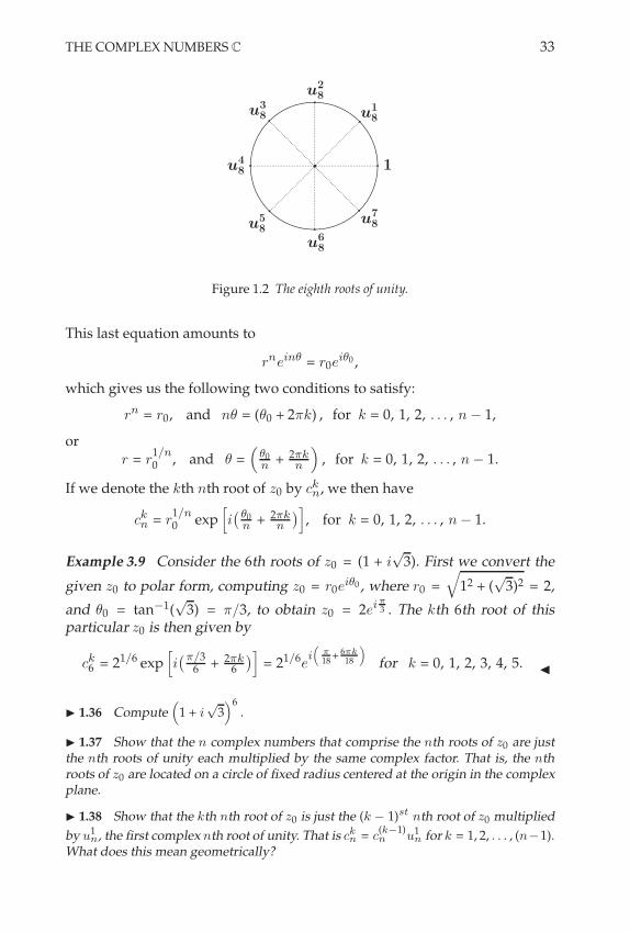
THE COMPLEX NUMBERS C 33
1
u2
8
u3
8
u4
8
u5
8
u6
8
u7
8
u1
8
Figure 1.2 The eighth roots of unity.
This last equation amounts to
rnein" = r0ei"0 ,
which gives us the following two conditions to satisfy:
rn = r0, and n$ = ($0 + 2%k) , for k = 0, 1, 2, . . . , n " 1,
orr = r
1/n0 , and $ =
("0n + 2$k
n
), for k = 0, 1, 2, . . . , n " 1.
If we denote the kth nth root of z0 by ckn, we then have
ckn = r
1/n0 exp
0i, "0
n + 2$kn
-1, for k = 0, 1, 2, . . . , n " 1.
Example 3.9 Consider the 6th roots of z0 = (1 + i,
3). First we convert the
given z0 to polar form, computing z0 = r0ei"0 , where r0 =
*12 + (
,
3)2 = 2,
and $0 = tan"1(,
3) = %/3, to obtain z0 = 2ei!3 . The kth 6th root of thisparticular z0 is then given by
ck6 = 21/6 exp
0i,$/3
6 + 2$k6
-1= 21/6e
i(!18 + 6!k
18
)
for k = 0, 1, 2, 3, 4, 5. "
! 1.36 Compute(
1 + i*
3)6
.
! 1.37 Show that the n complex numbers that comprise the nth roots of z0 are justthe nth roots of unity each multiplied by the same complex factor. That is, the nthroots of z0 are located on a circle of fixed radius centered at the origin in the complexplane.
! 1.38 Show that the kth nth root of z0 is just the (k & 1)stnth root of z0 multiplied
by u1n, the first complex nth root of unity. That is c
kn = c
(k!1)n u
1n for k = 1, 2, . . . , (n&1).
What does this mean geometrically?

34 THE SPACES R, Rk, AND C
! 1.39 Show that every quadratic equation of the form a z2 +b z+c = 0 where a, b, c "
C has at least one solution in C. Also show that if b2 & 4 a c %= 0, then the equation has
two solutions in C.
3.6 Matrix Representation of Complex Numbers
So far we have seen several different methods of representing a complexnumber, z # C. These include denoting z as an ordered pair (or two-dimensionalvector), using i notation, and polar notation. We present in this section yet an-other interpretation of z. While lacking in practical, computational benefits,it has a very nice conceptual upside. Complex numbers can be viewed asmatrices.
As we saw in the previous section, multiplication of one complex number byanother is geometrically equivalent to a scaling (stretching or shrinking) anda rotation in the complex plane. If we consider this process from the point ofview of transformations or mappings from C to C (or R2 to R2), the complexnumber we use as the “multiplier,” say, z0 = x0 + iy0, takes complex num-bers to complex numbers (or two-dimensional vectors to two-dimensionalvectors). We already know such multiplication is a linear operation, since
z0 (z1 + z2) = z0z1 + z0z2, and z0 (kz1) = kz0z1, for k a scalar.
Therefore, this multiplication operation is a linear transformation from C toC. Denote this linear transformation by Tz0 : C 3 C where Tz0 (z) = z0z,and recall from linear algebra that any linear transformation from one two-dimensional vector space to another can be represented by a 2.2 matrix A. Infact, given a specified basis for the vector spaces, this matrix representationis unique. In particular, consider the standard basis of C given by
{1, i} =
$21
0
3,
20
1
34.
Notice that we have expressed the complex number basis elements 1 and i bytheir corresponding two-dimensional column vectors, a notation with whichstudents of linear algebra should be familiar. Corresponding to this standardbasis, the unique standard matrix representation of Tz0 is given by
A =
5
66 6
Tz0 (1) Tz0(i)7 7
7
8 .
Therefore, the first column of A is given by
Tz0(1) = z01 = x0 + iy0 =
2x0
y0
3,
and the second column is given similarly by
Tz0 (i) = z0i = "y0 + ix0 =
2"y0
x0
3.

SUPPLEMENTARY EXERCISES 35
Overall we have
A =
9x0 "y0
y0 x0
:.
This is the unique matrix representation corresponding to Tz0 , and thereforeto z0, in the standard basis. This establishes a one-to-one correspondence be-tween the complex numbers and the set of 2 . 2 matrices with real entries of
the form
9a "bb a
:, i.e., we have
z = a + ib 83
9a "bb a
:.
We will refer to the collection of such 2 . 2 matrices as M.
! 1.40 Show that for z0 = x0 + iy0 " C, the product z0z can be computed via the
matrix product
9x0 &y0y0 x0
: (x
y
)for any z = x + iy " C.
! 1.41 Verify that any matrix in M represents a scaling and rotation of the vector itmultiplies.
! 1.42 Show that M forms a two-dimensional vector space, and that the mappingthat takes elements of C to elements of M is a one-to-one correspondence. This showsthat the class M of 2 + 2 matrices is isomorphic to the vector space of complex num-bers.
In this chapter we have focused primarily on the basic algebraic propertiesof the spaces R, Rk , and C, with some extra attention paid to the basic geom-etry of complex numbers as well. In the next chapter, we set out to expand oncertain shared, geometric features among all these spaces. In particular, eachof these spaces is a normed space. We will see that within each such space thenorm can be used to measure the “distance” between any pair of points. Sinceall norms share certain properties, what arises is a common framework forexploring what is referred to as the topology of such normed spaces. This inturn will provide the foundation for exploring certain distance-related prop-erties of interest to us in our development of analysis, such as open and closedsets, bounded and unbounded sets, convergence, and continuity, to name just afew. While this motivation for the study of the topology of spaces is not themost general, it is the most natural one for us to pursue in our study of anal-ysis on the Euclidean spaces of interest to us.
4 SUPPLEMENTARY EXERCISES
1. Show that Z is not a field.
2. Consider a subset A of a field F . If A is itself a field with the addition and multi-plication inherited from F , then A is called a subfield of F . Show that Q is a subfield

36 THE SPACES R, Rk, AND C
of R, and that there are no proper subfields of Q. This means that Q is the smallestsubfield of R.
3. Two fields F and G are said to be isomorphic if there exists a mapping f : F , G
that is one-to-one and onto such that for all a, b " F ,
(i) f (a + b) = f (a) + f (b),
(ii) f (ab) = f (a)f (b).
That is, f is a one-to-one correspondence between the elements of F and the elementsof G that also preserves the algebraic field properties. Note that the + on the left sideof the equality in (i) is the addition on F while the + on the right side is the additionon G, and similarly for the multiplications on each side of (ii), respectively. Show thatC is not isomorphic to R by considering the following:
a) Assume f : C , R possesses the above isomorphism properties.
b) Determine f (0).
c) Determine f (1).
d) Use the fact that i2 = &1 to obtain a contradiction.
4. Show that for all a, b, c " R,
a) & (&a) = a b) (a!1)!1 = a for a %= 0c) a(&b) = (&a)(b) = &(ab) d) (&a)(&b) = ab
e) ab = 0 - a = 0 or b = 0 f) a + b = a + c - b = c
g) a + b = a - b = 0 h) a + b = 0 - b = &a
i) a %= 0 and ab = ac - b = c j) a %= 0 and ab = a - b = 1k) a %= 0 and ab = 1 - b = a
!1 l) 0a = 0
5. Find the multiplicative inverse for each of the following complex numbers.
a) i b) 7i c) 3 + i d) 5 & i e)*
2 & #
2 i
6. Express each of the following complex numbers in x + i y form.
a) 13+i
b) 1+i"2!!
2 ic) 2i
5!id) e!#i
7i
e) (1 + 2i)('i) f) (7 + 'i)(' + i) g) (1 + 4i)(4 & 2i)
7. Suppose a and b are real numbers such that 0 # a # b.
a) Show that a2 # b
2. b) Show that*
a #*
b.
8. Can you define another ordering for R2 different from the one described on page 13?
How about one defined in terms of polar coordinates?
9. Suppose you were to attempt to define an ordering on R2 in the following way:
“Given two vectors x and y in R2, if x1 < y1 and x2 < y2 we will write x < y and say
that x is “less than” y." What is wrong with this attempt?
10. Define an ordering for R3. How about more generally for R
k?

SUPPLEMENTARY EXERCISES 37
11. Is there a “well-ordered property of R” ? What about for Rk? How about C?
(Answer: There is none. Explain this.)
12. Show that Q is not complete according to the Dedekind completeness property.
13. Suppose q " Q. If # " R is irrational, show that q + # is irrational.
14. Suppose a and b are two arbitrary real numbers. Simplify the expressions 12
,a +
b +&& a & b
&&- and 12
,a + b &
&& a & b&&-.
15. Suppose a square root of a complex number z is a complex number w such thatw
2 = z. Find the two square roots of 1+i. How do you know there are only two squareroots? Find the only complex number having only one square root.
16. Find the complex solutions to the equation z2+z+1 = 0. Show that every quadratic
equation az2 + bz + c = 0 where a, b, c " C has a solution if a %= 0. How is this different
from the real case ax2 + bx + c = 0 with a, b, c " R?
17. Define what it means for w " C to be a fifth root of z. How many fifth roots does32 have if complex numbers are allowed as roots? Graph the fifth roots of 32. Whatgeometrical shape is associated with your graph? Why?
18. Express the following in x + i y form: a) (1 + i)100 b) (*
3 & i)50
19. Suppose z " C is on the circle of radius two centered at the origin. Show that13 #
&& z + 12 z
5 + 1&& # 19.
20. Let zi " C for i = 1, 2, . . . , m. Show that&&;m
i=1 zi
&& #;
m
i=1 |zi|.
21. If z " C is such that |z| = 1, compute&&1 + z
&&2 +&&1 & z
&&2.
22. If (·, ·) is an inner product on Rk , show that (0, x) = 0 for all x " R
k .
23. Show that for any real numbers a, b, c, d, the following is true:
&*,
a2 + b2-,
c2 + d2-# ac & bd #
*,a2 + b2
-,c2 + d2
-.
(Hint: Use the Cauchy-Schwarz inequality.)
24. Let (·, ·) be an inner product on Rk , and let B =
!x " R
k : |x| < 1"
where | · | is
the induced norm. Show that B is convex, i.e., that for all x, y " B, the line segmentin R
k that joins x to y is contained in B.
25. Show that for all x and y in R,&& x + y
&&2 +&& x & y
&&2 = 2 |x|2 + 2 |y|2,
andx y = 1
4
0&& x + y&&2 &
&& x & y&&21
.
The first equality is called the parallelogram equality. The second is called the polar-ization identity.

38 THE SPACES R, Rk, AND C
26. Consider Rk with the dot product as inner product. Show that for any x, y " R
k ,
|x + y|2 + |x & y|2 = 2 |x|2 + 2 |y|2
andx · y = 1
4
0|x + y|2 & |x & y|2
1.
These are the parallelogram equality and the polarization identity, respectively, forthe dot product and its induced norm on R
k. The significance of these two equalitieslies in the following fact, described more generally in terms of an arbitrary norm. Ifa norm on R
k satisfies the parallelogram equality, then an inner product that inducesthat norm can be defined according to the polarization identity (just replace x · y inthe above equality with (x, y)). If the norm fails to satisfy the parallelogram equality,then no such inducing inner product exists for that norm.
27. Suppose (·, ·) is an arbitrary inner product on Rk , and let | · | be the associated
induced norm. Show that the polarization identity and the parallelogram equality
hold, i.e., for all x, y " Rk ,
|x + y|2 + |x & y|2 = 2|x|2 + 2|y|2, and (x, y) = 14
0|x + y|2 & |x & y|2
1.
28. For all x = (x1, x2) " R2, consider the norm on R
2 given by |x|1 = |x1| + |x2|. Doesthis norm satisfy the parallelogram equality on R
2?
29. Suppose | · | is an arbitrary norm on Rk satisfying the parallelogram equality,
|x + y|2 + |x & y|2 = 2 |x|2 + 2 |y|2
for all x, y " Rk . Show that the inner product defined by
(x, y) . 14
0|x + y|2 & |x & y|2
1
for all x, y " Rk is a valid inner product that induces this norm. To do so, show
a) 0 # (x, x) = |x|2 for all x " Rk .
b) (y, x) = (x, y) for all x, y " Rk .
c) (x + y, z) = (x, z) + (y, z) for all x, y, z " Rk .
d) (x, cy) = c (x, y) for all x, y " Rk and for all c " R. To establish this, consider the
following special cases, in order: c = n " Z+, c = &n " Z
!, c = 1m
for nonzero
m " Z, c = n
mfor nonzero m " Z and n " Z, c = r " Q. This step-by-step
procedure proves the result for rational c. Finally, to establish the result for any
real c, show that&&(x, cy) & c (x, y)
&& < $ for all $ > 0. To do this, consider that&&(x, cy) & c (x, y)
&& =&&&(x, (c & r)y) + (x, ry) & r (x, y) + (r & c) (x, y)
&&&,
where r " Q and |c & r| can be made as small as you like.
e) Show that | · | is induced by this inner product.
30. Is the norm | · |1 described in Example 2.6 on page 17 induced by an inner productin R
2?

SUPPLEMENTARY EXERCISES 39
31. What is the geometrical significance of the parallelogram equality in R2?
32. Consider the dot product induced norm | · | and | · |1 from Example 2.6 on page17, both defined on R
2. Show that
12 |x|1 # |x| # 2 |x|1 for every x " R
2.
In general, any two norms | · |1 and | · |2 that satisfy "!1|x|1 # |x|2 # " |x|1 for " > 0
are called equivalent. It can be shown that any two norms on Rk are equivalent. This
fact might surprise one at first. We will see in Chapter 3 that it is a very significant,and convenient truth.
33. For z, w " C, define the product (·, ·) : C + C , C by
(z, w) . z w.
Recall that the inner product properties in Definition 2.1 on page 14 were specifiedfor real vector spaces. Is the product we define in this exercise an inner product on C
according to Definition 2.1 of the last subsection? If so, verify it. If not, can you thinkof a way to extend Definition 2.1 so as to include the product of this exercise whileremaining consistent with the original definition when the vectors used are, in fact,real vectors?
34. Recall that C is a geometric copy of R2. Verify that the norm | · | in C defined in
equation (1.6) on page 25 is just another way of writing the induced norm from R2
under the R2 dot product. Is this complex norm induced by an associated complex
inner product? If so, what inner product on C induces it?
35. For the norm | · | in C defined by (1.6) on page 25, and the complex inner productgiven by (z, w) . z w, show the following:
a)&& z + w
&&2 +&& z & w
&&2 +&& z + iw
&&2 +&& z & iw
&&2 = 4 |z|2 + 4 |w|2
b) Re,(z, w)
-= 1
4
,|z + w|2 & |z & w|2
-
c) Im,(z, w)
-= 1
4
,|z + iw|2 & |z & iw|2
-
d) (z, w) = 14
,|z + iw|2 & |z & iw|2
-+ i
14
,|z + iw|2 & |z & iw|2
-
Part a) is the parallelogram equality, and part d) is the polarization identity for thiscomplex inner product.
36. Let C2 =
.(z, w) : z, w " C
/, and define
<(z1, w1), (z2, w2)
=. z1w1 + z2w2.
Show that (·, ·) is an inner product on C2 with the complex numbers as scalars. What
is the norm induced by this inner product?
37. Consider C2 with the inner product described in the last exercise. Find an associ-
ated Cauchy-Schwarz inequality.
38. Find arg z and Arg(z) for the following:

40 THE SPACES R, Rk, AND C
a) z = &i b) z = &1 + i c) z = 1 + i*
3
39. For the following pairs of complex numbers, show that arg z1z2 = arg z1 + arg z2.
a) z1 = &3, z2 = 7 i b) z1 = 1 & i, z2 = 1 + i*
3 c) z1 = 1 & i, z2 = 1 + i
40. For parts a), b), and c) of the previous exercise, determine whether or not Arg(z1z2) =Arg(z1) + Arg(z2).
41. Suppose n " N, n > 1. Prove that
n!1+
j=0
e2!in j = 0.
(Hint: Set the value of that sum to be s, and consider e2!in s. Or use the geometric
series.)

2POINT-SET TOPOLOGY
Mathematics would certainly have not come into existence if one had known fromthe beginning that there was in nature no exactly straight line, no actual circle, noabsolute magnitude.
Friedrich Nietzsche
To someone unfamiliar with the subject, the topology of spaces such as R, Rk ,or C can be a difficult concept to describe. Our desire in this introductorynote is only to motivate our study of certain topological topics as they re-late to analysis. The chapter itself will serve to make these ideas more pre-cise. Also, it is worth emphasizing that many topological results applicableto more general spaces (that is, to spaces other than R, Rk , and C) belongmore properly to the subject of topology itself, not analysis, and so we willnot pursue them. With these goals in mind, our motivation for the study oftopology stems from the following fact: It will be useful in our work to char-acterize the points of a space in certain ways. In particular, if A is any subsetof one of the spaces R, Rk , or C, we will characterize the points of the spacerelative to A. That is, we will define a collection of properties that describein some way how the points of A are configured relative to each other, andto the points of the space outside of A. We will collectively refer to the studyof such properties as point-set topology. It is both significant and convenientthat within the spaces R, Rk , and C, these properties can be described in re-lation to the distances between points. It is just as significant and convenientthat each of these spaces is a normed space, and that within each of them wecan specify the distances between points using the norm on each space. Thisshared trait will allow us to efficiently characterize the topological featuresof these spaces in terms that are common to all of them. For this reason, wewill use the symbol X throughout our discussion to represent any one of thespaces R, Rk , or C when the result to which we refer applies to each of them.If a result is unique to one of the spaces R, Rk , or C or does not apply to oneof them, we will make explicit mention of that fact.
41

42 POINT-SET TOPOLOGY
1 BOUNDED SETS
We begin by developing the concept of distance between elements of a spaceX. We remind the reader that, as noted in the introduction to this chapter, wewill generally limit our attention to the sets R, Rk, and C. As we saw in theprevious chapter, each of these spaces is a normed space. Since most of theresults of interest to us will apply to all of them, we will let X be our concisenotation for any (or all) of these spaces in statements that apply to them all.With this convention in mind, we note that the norm associated with a spaceis a convenient means for measuring distances between points in that space.1
This motivates the following definition:
distance between x and y in X / |x " y |.
Here, | · | is the usual norm associated with the space X unless otherwisespecified. This distance function inherits many of the norm properties, andwe list these now: For all x, y # X,
(i) |x " y | ! 0 with equality if and only if x = y.
(ii) |x " y | = | y " x |.
(iii) |x " y | + |x " z | + | z " y | for any z # X.
To better suggest the geometric intuition associated with the notion of “dis-tance” on normed spaces such as X, the elements of X are often referred to aspoints.
1.1 Bounded Sets in X
We will now develop certain concepts and their associated language for de-scribing collections of points in X. We start by defining what it means for asubset A ' X to be bounded in X.
Definition 1.1 The set A ' X is called bounded if there exists a nonnegativereal number M such that |x | + M for each x # A.
In the above definition, it sometimes helps to remember that |x | = |x " 0 |and is the distance from x to 0 in X. With this in mind, a bounded set can bethought of as one that can be entirely contained inside a disk centered at theorigin and of large enough finite radius. The following examples illustratethe above definition in the spaces of interest to us.
Example 1.2 Let A = {x # R : |x " 4 | < 2} . Clearly A is bounded, since for
1The function that measures distance in a given space can be defined in other ways as well.It is convenient when the distance function is induced by a norm in the space, but it is notnecessary. The reader can see another kind of distance function in the supplementary exercisesat the end of this chapter.

BOUNDED SETS 43
each x # A we have |x | + |x " 4 | + 4 < 6. Letting M = 6 in Definition 1.1gives the result. The set A consists of those points within R that are within adistance 2 of the point 4. "
Example 1.3 Let A =!
5n2n"1 : n # N
"' R. We will show that A is bounded.
Note that each x # A satisfies
|x | =
&&&&5n
2n" 1
&&&& =5n
2n " 1+
5n
n= 5.
Letting M = 5 in Definition 1.1 gives the result. "
Example 1.4 Consider the first quadrant Q1 ' R2. We will show that Q1 isnot bounded using Definition 1.1 and a proof by contradiction. To this end,assume there exists a real number M ! 0 such that
|x | + M for all x # Q1.
Choosing x = (n, n) where n # N, we then have
|x | =,
2 n + M for all n # N.
This is clearly a contradiction. (Why?) "
Example 1.5 Let A = {z # C : | z | + | 1 " z | = 5} . We will show that A isbounded. Let z be an arbitrary element of A. Then | z | + | 1 " z | = 5. But| z " 1 | ! | z |" 1 (Why?), and so we have
| z | + | z |" 1 + | z | + | 1 " z | = 5,
which implies | z | + 3. Since z # A was arbitrary, letting M = 3 in Defini-tion 1.1 yields the result. Note that the points in the set A are those on theellipse centered at z = 1/2, with foci at z = 0 and z = 1, in the complex plane.One could also argue as follows. If |z|+ |1 " z| = 5, then clearly |z| + 5. Hencefor all z # A, |z| + 5. This also shows that A is bounded, although the boundM we get is larger than before. "
! 2.1 Determine whether the given set is bounded or unbounded.
a) S =.z " C : |z| + |z & 1| < |z & 2|
/
b) S =.z " C : |z| + |z & 1| > |z & 2|
/
c) S =.xn " R
3 : xn =,n
22!n, n2+1
2n3+1 , cos n"n
-/
! 2.2 Consider a set S ! X.a) If S is bounded, show that the complement of S, denoted by S
C , is unbounded.
b) If S is unbounded, show that SC is not necessarily bounded.
! 2.3 Suppose {S!} ! X is a collection of bounded sets.
a) Is#
S! bounded? b) Is>
S! bounded? (Answers: a) Depends, b) Yes. For a),the answer is always yes if the collection is finite.)
In the following subsection, we consider the important case of bounded setsin R. The real numbers possess special order properties that give rise to no-tions of boundedness not found in Rk or C.

44 POINT-SET TOPOLOGY
1.2 Bounded Sets in R
Because R possesses a “natural” ordering that plays a significant role in char-acterizing the real numbers, there are several concepts associated with bound-edness in this case that require special attention.
Upper Bounds and Lower Bounds
We begin with a definition.
Definition 1.6 A set of real numbers S is said to be bounded above if thereexists a real number M such that s + M for all s # S. Such a number M iscalled an upper bound on S.
Sets of real numbers can have more than one upper bound, or no upperbound, as the following example illustrates.
Example 1.7
a) Consider the set R" of negative real numbers. Any nonnegative real num-ber M ! 0 serves as an upper bound for R".
b) Consider the set of all real numbers R. This set is not bounded above.To see this, assume M is an upper bound on R. Then, since M + 1 is anelement of R greater than M , we have a contradiction. Hence, no suchupper bound exists.
c) Suppose we generate a set of real numbers A according to the followingalgorithm. Let x1 = 1 and xn+1 = 2 +
,
xn for n ! 1. That is,
A =.
1, 2 +,
1, 2 +
*2 +
,
1, . . ./
.
We will show that A is bounded above. To do this, we will establish thatxn + 4 for all n ! 1 by induction. This is obviously true for n = 1. Nowassume that xN + 4. We have then,
xN+1 = 2 +,
xN + 2 +,
4 = 4,
and the claim is proved. "
A lower bound for a set of real numbers is defined in a manner similar to thatof an upper bound.
Definition 1.8 A set of real numbers S is said to be bounded below if thereexists a real number m such that m + s for all s # S. Such a number m iscalled a lower bound on S.
Example 1.9
a) The set of positive real numbers R+ is bounded below. Any nonpositivereal number m + 0 serves as a lower bound on R+.

BOUNDED SETS 45
b) The set of real numbers R is not bounded below. For any assumed lowerbound m, consider the real number m " 1.
c) Let A =!
("1)nnn+1 : n # N
". To show that A is bounded below, we note that
if n is even, then ("1)nnn+1 = n
n+1 ! 0, and if n is odd, then ("1)nnn+1 = "
nn+1 !
"1. Therefore, ("1)nnn+1 ! "1 for every n # N. "
! 2.4 Prove that a set of real numbers S is both bounded above and bounded belowif and only if it is bounded.
! 2.5 Show that the set A described in each part c) of the previous two examples isbounded.
The Least Upper Bound and the Greatest Lower Bound
Suppose a set of real numbers is bounded above. If we consider the collectionof all upper bounds of this set, it is reasonable to ask whether there is a leastupper bound from this collection of upper bounds.
Definition 1.10 For a nonempty set of real numbers S ' R, the real numberMS is called the least upper bound, or the supremum, or the sup of the setS, if the following both hold:
(i) MS is an upper bound on S,(ii) MS + M for all upper bounds M of S.
In this case, we write MS = sup S.
It follows at once from the definition that sup S, if it exists, is unique. In fact,suppose both MS and M &
S satisfied the above properties. Then both are upperbounds for S, and so we get MS + M &
S and M &S + MS by the second axiom.
Hence MS = M &S .
Likewise, if a set S is bounded below, it is reasonable to ask whether there isa greatest lower bound for S.
Definition 1.11 For a nonempty set of real numbers S ' R, the real numbermS is called the greatest lower bound, or the infimum, or the inf of the setS, if the following both hold:
(i) mS is a lower bound on S(ii) m + mS for all lower bounds m of S.
In this case, we write mS = inf S.
Similarly, inf S is unique if it exists.
Of course, merely defining the properties of a new mathematical object doesnot, in itself, ensure its existence. Also, it is important to note that if either

46 POINT-SET TOPOLOGY
the sup or the inf of a set S exists, it may or may not be a member of theset S. “Having a sup” does not necessarily mean that sup S is a member ofthe set S, but only that the sup exists. Likewise for the inf. The followingimportant theorem tells us when we are guaranteed the existence of a sup oran inf. As the proof will show, their existence is a direct consequence of thecompleteness of R.
Theorem 1.12 If S is a nonempty set of real numbers that is bounded above, thensup S exists. If S is a nonempty set of real numbers that is bounded below, then inf Sexists.
PROOF We prove the case where S is nonempty and bounded above, leav-ing the bounded below case as an exercise. Let B be the set of all upperbounds on S, and let A = BC . Then R = A % B, and a < b for all a # Aand for all b # B. (Why?) Since A and B satisfy our Dedekind completenessproperty criteria, either A has a maximal element or B has a minimal ele-ment. Suppose A has a maximal element, '. Then ' $# B, so ' is not an upperbound for S, i.e., there exists s # S such that ' < s. Since this is a strict in-equality, there must exist a real number between ' and s. In fact, c / ('+s)/2is such a real number, and so ' < c < s. But c < s implies c $# B, i.e., c # A.Since ' < c, we have a contradiction, since ' # A was assumed to be thelargest element of A. Therefore, since our completeness criteria are satisfied,and A does not have a maximal element, it must be true that B has a minimalelement, call it (. Clearly ( is the least upper bound or sup S. #
! 2.6 Complete the proof of the above theorem. That is, suppose S is a nonemptyset of real numbers that is bounded below, and show from this that inf S exists.
Example 1.13 Let S =!
("1)n nn+1 : n # N
"=!"
12 , 2
3 ," 34 , 4
5 , . . ."
. We will show
that MS = sup S = 1. To do this, we begin by noting that
("1)n n
n + 1+
n
n + 1+ 1 for all n.
Therefore, 1 is an upper bound for S. To show that 1 is the least upper boundfor S, we assume there is a smaller upper bound M such that
("1)n n
n + 1+ M < 1 for all n.
To get a contradiction, it suffices to find an even integer n such that M <n
n+1 < 1. This is equivalent to finding an even integer n > M1"M , which is
certainly possible according to the Archimedean property. Therefore, MS =sup S = 1. "
! 2.7 For the set S of the previous example, show that mS = inf S = &1.

BOUNDED SETS 47
! 2.8 Recall that a maximal element of a set S is an element x " S such that s # x
for all s " S. Likewise, a minimal element of a set S is an element y " S such thaty # s for all s " S. When they exist, we may denote a maximal element of a set S
by max S, and a minimal element of a set S by min S. Show that if S has a maximalelement, then max S = sup S. Likewise, show that if S has a minimal element, thenmin S = inf S.
The following proposition involving properties of sups and infs will be ofmuch use to us in our work. The proof follows readily from the definitionsof supremum and infimum and is left to the reader.
Proposition 1.14 Let MS = sup S and let mS = inf S for some set S of realnumbers.
a) For every u < MS there exists s # S such that u < s + MS .
b) For every v > mS there exists s # S such that mS + s < v.
! 2.9 Prove the above proposition.
! 2.10 Use Proposition 1.14 to show that if sup S exists for S ! R, then sup S isunique. Do likewise for inf S.
1.3 Spheres, Balls, and Neighborhoods
Among the simplest types of bounded set, and among the most useful inanalysis, are spheres, balls, and neighborhoods.
Spheres
Consider a point x0 in X. Now consider all other points x # X that lie a dis-tance r from x0. We call this collection of points the sphere of radius r centeredat x0. More formally, we state the following definition.
Definition 1.15 For x0 in X, and for any r > 0, the collection of points x # X
satisfying |x " x0 | = r is called the sphere of radius r centered at x0.
In most cases in which we will work, the intuition provided by thinking of asphere as the familiar object from three-dimensional geometry is a valuableaid in understanding and in problem solving. Nonetheless, spheres need notbe round, even in our familiar spaces R, Rk , and C. (For r > 0 fixed, what,after all, is the sphere of radius r in R?)2
2In fact, since the definition of sphere depends directly on the norm being used to measuredistance, and since there are many possible norms for any normed space, the intuitive notion of“sphere” can become somewhat distorted. We will not have need of such counterintuitive casesin our development of analysis, but refer to Example 2.6 on page 17 of Chapter 1 for a norm thatinduces a distance function with nonround spheres.
48 POINT-SET TOPOLOGY
Example 1.16 As already seen in Chapter 1, polar notation and the usualnorm give us an especially easy way to describe spheres in C (although inChapter 1 they were referred to as circles). Recall that we considered theequation of such a sphere of radius R > 0 centered at the origin in C bythe simple equation | z " 0 | = | z | = R. We saw that the sphere of radius Rcentered at z0 = x0 + iy0 is given by points z = x + iy in the plane C satisfyingthe equation
| z " z0 | = R.
Note that any point z # C that satisfies this equation also satisfies z " z0 =R ei" for some angle $ (after all, the complex number w / z " z0 is such thatits magnitude is R, and its argument is as yet unspecified), and so the pointsz on this sphere are those points satisfying
z = z0 + R ei", for 0 + $ < 2%. "
Balls
We now give the definitions of an open ball and a closed ball in X.
Definition 1.17 Consider a point x0 in X, and let r > 0 be fixed.
1. The collection of points x # X satisfying |x " x0 | < ris called the open ball of radius r centered at x0.
2. The collection of points x # X satisfying |x " x0 | + ris called the closed ball of radius r centered at x0.
Like the sphere, the intuitive notion of “ball” is directly dependent on thenorm used in the space X.
Example 1.18 Consider the set of real numbers described by A = {x # R :|x " 1 | < 2} and B = {x # R : |x + 1 | + 3}. The set A is an open ball ofradius 2 centered at x = 1, and the set B is a closed ball of radius 3 centeredat x = "1. "
Of course, as the previous example illustrates, open and closed balls in R
with the usual distance are just open and closed intervals, respectively. Thesituation in Rk is similarly straightforward. In fact, using the usual distanceon Rk , the open ball of radius r centered at ! = ()1, . . . , )k) # Rk is given bythose x = (x1, . . . , xk) # Rk satisfying |x " !| < r, or, equivalently,
(x1 " )1)2 + · · · + (xk " )k)2 < r2,
and the closed ball of radius r centered at ! # Rk is given by those x # Rk
satisfying |x " !| + r, or, equivalently,
(x1 " )1)2 + · · · + (xk " )k)2+ r2.

BOUNDED SETS 49
Finally, open and closed balls in the complex plane C are easy to describe.The open ball of radius r centered at z0 # C is given by the set of pointsz # C satisfying
| z " z0 | < r,
and the closed ball of radius r centered at z0 is given by the set of points zsatisfying
| z " z0 | + r.
Neighborhoods
For a fixed point x0 in X, open balls provide a precise and intuitive way todescribe the part of X that “surrounds” the point x0. In fact, two differenttypes of open ball will be of interest to us in our work, and we define themnow. Their use in referring to that portion of X that surrounds a specifiedpoint x0 is reflected in their names—they are called neighborhoods of x0.
Definition 1.19
1. A neighborhood of x0 # X is an open ball of radius r > 0 in X
that is centered at x0. Such a neighborhood is denoted by Nr(x0).
2. A deleted neighborhood of x0 # X is an open ball of radius r > 0in X that is centered at x0 and that excludes the point x0 itself.Such a deleted neighborhood is denoted by N &
r(x0).
To illustrate the above definition, consider the following sets in R :
N 12(3) =
!x # R : |x " 3 | < 1
2
",
andN &
12
(3) =!
x # R : 0 < |x " 3 | < 12
".
The first set, the neighborhood of radius 12 centered at x = 3, is just the open
interval,
52 , 7
2
-centered at x = 3. The second set, the deleted neighborhood of
radius 12 centered at x = 3, consists of the union
,52 , 3
-%
,3, 7
2
-. For an example
in R2, consider the following sets relative to the point x0 = (3, 1) :
N1(x0) =!x # R
2 : |x" x0 | < 1"
=!
(x1, x2) # R2 :
*(x1 " 3)2 + (x2 " 1)2 < 1
",
N &1(x0) =
!x # R
2 : 0 < |x " x0 | < 1"
=!
(x1, x2) # R2 : 0 <
*(x1 " 3)2 + (x2 " 1)2 < 1
".
The first set, the neighborhood of radius 1 centered at x0 = (3, 1), is the inte-rior of the disk of radius 1 centered at x0. The second set, the deleted neigh-

50 POINT-SET TOPOLOGY
borhood of radius 1 centered at x0 = (3, 1), is the “punctured” interior of thedisk of radius 1 centered at x0 that excludes x0 itself.
! 2.11 Recall that any interval of real numbers contains infinitely many rational andinfinitely many irrational numbers. Therefore, if x0 is a real number, then every neigh-borhood Nr(x0) centered at x0 contains infinitely many rational and infinitely manyirrational numbers. Let A and B be subsets of R
2 defined as follows:
A =!
(x, y) " R2 : x, y " Q
"and B =
!(x, y) " R
2 : x, y " I
".
That is, A consists of those vectors from R2 having only rational components, and B
consists of those vectors of R2 having only irrational components. If x0 is an arbitrary
vector in R2, show that every neighborhood Nr(x0) centered at x0 contains infinitely
many elements of A and infinitely many elements of B. Investigate the comparablesituation in R
k and in C.
2 CLASSIFICATION OF POINTS
2.1 Interior, Exterior, and Boundary Points
The concept of neighborhood allows us to characterize any point x0 in X in avery convenient way. In particular, consider an arbitrary set A ' X. Then anypoint in X can be unambiguously classified according to its relation to the setA.
Definition 2.1 For a given set A ' X, a point x # X is called
1. an interior point of A if there exists a neighborhood of x that isentirely contained in A.
2. an exterior point of A if there exists a neighborhood of x that isentirely contained in AC .
3. a boundary point of A if every neighborhood of x contains a pointin A and a point in AC .
For a given set A ' X, each point x # X must satisfy exactly one of theproperties described in the previous definition; each point x # X is an interiorpoint of A, an exterior point of A, or a boundary point of A, the designationbeing mutually exclusive of the other two possibilities.
! 2.12 Prove the above claim in the following two steps: First, consider an arbitrarypoint in X and show that it must satisfy at least one of the above three characteriza-tions. Then, prove that if a point in X satisfies one of the above three characterizations,it cannot satisfy the other two.

CLASSIFICATION OF POINTS 51
Definition 2.2 A given set A ' X implicitly defines the following three sub-sets of X :
1. the boundary of A, denoted by *A, and consisting of all theboundary points of A,
2. the interior of A, denoted by Int(A), and consisting of all theinterior points of A,
3. the exterior of A, denoted by Ext(A), and consisting of all theexterior points of A.
Example 2.3 Consider the closed ball in R2 centered at x0 = (1, 2) and givenby A =
.x # R2 : |x " x0 | + 5
/. We will show that
a) the point x1 = (1, 3) is an interior point of A.
b) the point x2 = (7, 2) is an exterior point of A.
c) the point x3 = (1, 7) is a boundary point of A.
These classifications are easily determined by considering Figure 2.1 below.However, pictures are not sufficient, and in many cases not easily drawn orinterpreted, as a means for properly classifying points. In what follows, foreach point, we apply the relevant definition to establish the proper charac-terization.
x0 x2
x3
"A
x1Int(A)
Ext(A)
Figure 2.1 A set with interior, exterior, and boundary points.
To establish a), consider N 12(x1). We will show that N 1
2(x1) ' A. To see this,

52 POINT-SET TOPOLOGY
let x # N 12(x1). Then |x " x1 | < 1
2 . Now it follows that
|x " x0 | + |x" x1 | + |x1 " x0 | < 12 + 1 < 5,
and therefore x # A. To establish b), consider N 14(x2). We will show that
N 14(x2) ' AC . To see this, let x # N 1
4(x2). Then |x " x2 | < 1
4 . From this we
have
|x " x0 | =&&&x " x2 + x2 " x0
&&&
=&&&x " x2 + (6, 0)
&&&
! 6 " |x " x2 |
> 6 "14 > 5.
Therefore, x # AC . To establish c), we will show that every neighborhoodcentered at x3 contains at least one point in A and at least one point in AC .To do this, we consider the case of neighborhoods having radius 0 < r < 1first. Let Nr(x3) be an arbitrary such neighborhood centered at x3. Note that
x = x3 "
,0, r
2
-# A & Nr(x3),
and thatx = x3 +
,0, r
2
-# AC
& Nr(x3).
Since the neighborhood Nr(x3) was an arbitrary neighborhood centered atx3 having radius 0 < r < 1, all such neighborhoods must also contain atleast one point in A and at least one point in AC . We leave as an exercise thetask of proving that any neighborhood centered at x3 having radius r ! 1also contains at least one point in A and at least one point in AC , and thattherefore x3 is a boundary point of A. Note that the boundary of A is givenby *A = {x # R2 : |x " x0| = 5} and consists of those points on the circleof radius 5 centered at x0. The interior of A is given by Int(A) = {x # R2 :|x" x0| < 5}, and is the open disk of radius 5 centered at x0. The exterior ofA is the set Ext(A) = {x # R2 : |x " x0| > 5} and consists of all points of R2
outside the disk of radius 5 centered at x0. "
! 2.13 Complete part (iii) of the previous example by showing that Nr(x3) for r ' 1
must contain at least one point in A and at least one point in AC .
! 2.14 For A ! X, show that (A = (
(A
C
).
It is an interesting fact that within the space of real numbers R, every pointof Q is a boundary point of Q, i.e., Q ' *Q. To see this, consider any pointq0 # Q. Then, for any real number r > 0 the neighborhood Nr(q0) mustcontain both rational and irrational numbers. Hence, q0 is a boundary pointof Q. Perhaps even more interesting is the fact that the boundary of Q is allof R.
! 2.15 Show that (Q = R. Show the same for (I.

CLASSIFICATION OF POINTS 53
2.2 Limit Points and Isolated PointsLimit Points
For a subset A of X, we have seen that any point x # X is exactly one ofthe following three types: an interior point of A, an exterior point of A, or aboundary point of A. There is another classification of interest to us. For anysubset A of X, a point x # X might also be what is referred to as a limit point3
of A. We formalize this important concept in the following definition.
Definition 2.4 Let A ' X. Then x0 # X is called a limit point of A if N &r(x0)&
A $= ! for all r > 0, i.e., if every deleted neighborhood of x0 contains at leastone point of A.
! 2.16 Show that, in fact, if x0 is a limit point of A, then every deleted neighborhoodof x0 contains infinitely many points of A.
! 2.17 Show that if x0 " X is not a limit point of A ! X, then x0 is a limit point ofA
C .
For any set A ' X, we have seen that there are two ways of classifying x0 # X
with respect to A. First, x0 must be an interior point, an exterior point, or aboundary point of A. Second, x0 can be a limit point of A, or not a limitpoint of A. One might wonder if there is a relationship between these twoclassifications. The following examples give a partial answer to this question.
Example 2.5 Consider A ' X and suppose x0 is an interior point of A. Wewill show that x0 is also a limit point of A. To do this, note that since x0
is an interior point of A, there exists a neighborhood Nr(x0) ' A for somer > 0. Let N &
%(x0) be any deleted neighborhood of x0. There are two cases toconsider: + + r and + > r. The first leads to N%(x0) ' Nr(x0) ' A, while thesecond leads to Nr(x0) ' N%(x0). In both situations there are clearly infinitelymany points of A inside of N &
%(x0), and so x0 is a limit point of A. "
Example 2.6 Let A =!
1n : n # N
"' R. We will show that 0, a boundary
point of A that is not a member of A, is a limit point of A. To this end, considerNr(0) for any r > 0, and choose an integer M > 1
r (How do we know we can
do this?). Then 0 < 1M < r, and so 1
M # N &r(0). But 1
M # A, and sincer > 0 was arbitrary, this shows that there is at least one element of A in everydeleted neighborhood of 0. Hence 0 is a limit point of A. "
Example 2.7 Let A =.x # R2 : |x | + 1
/. We will show that x0 = (0, 1), a
boundary point that is an element of A, is a limit point of A. To this end, we
3Some texts also use the term accumulation point or cluster point in addition to limit point.In fact, some authors use two of these three terms to distinguish between two situations: limitpoints of sequences of numbers and limit points of sets of points. We choose to use the singleterm limit point for both cases. The context is typically sufficient to clarify the interpretation.

54 POINT-SET TOPOLOGY
first consider an arbitrary neighborhood N &r(x0) for any 0 < r < 1 (the r ! 1
case will be handled separately). Choose x2 such that 1 " r < x2 < 1. Thenx = (0, x2) # N &
r(x0) & A. Now consider an arbitrary neighborhood Nr(x0)with r ! 1. In this case, any x = (0, x2) with 0 < x2 < 1, is in N &
r(x0) & A.Since every deleted neighborhood of x0 has been shown to contain at leastone point of A, x0 is a limit point of A. "
! 2.18 It is not necessarily true that if x is a boundary point of a subset A of X, thenx must be a limit point of A. Give a counterexample.
! 2.19 Suppose x0 is an exterior point of A ! X. Then show that x0 can never be alimit point of A. But show that x0 is necessarily a limit point of A
C .
While it is useful to be able to identify individual points as limit points for agiven set, it will also be useful to consider the collection of all the limit pointsassociated with a given set. We formally define this collection of points now.
Definition 2.8 The collection of limit points of A ' X is denoted by A& andis called the derived set of A.
Example 2.9 We will show that Z& = !. To this end, suppose x0 # Z&. Wewill obtain a contradiction. Note that the point x0 cannot be an integer, sinceif it were, N &
12
(x0) & Z = !, contradicting that x0 is a limit point. Therefore x0
must be in ZC . But for x0 # ZC , there exists M # Z such that M < x0 < M +1.Taking r < min
.|x0 "M |, |x0 " (M + 1) |
/obtains a neighborhood N &
r(x0)such that N &
r(x0) & Z = !. Since this contradicts our assumption that x0 is alimit point of Z, we must have that Z& = !. "
Example 2.10 We will show that Q& = R. To this end, let x0 be an arbitraryreal number, and consider any deleted neighborhood N &
r(x0). Since there mustbe a rational number between x0 and x0+r (Why?), it follows that N &
r(x0)&Q $=!, and so x0 is a limit point of Q. Since x0 was arbitrary, Q& = R. "
! 2.20 If A ! B ! X, show that A# ! B
#.
Isolated Points
We now define the concept of an isolated point.
Definition 2.11 For A ' X, a point x # A is called an isolated point of A ifthere exists r > 0 such that N &
r(x) & A = !.
That is, x # A is an isolated point of A if and only if there exists a deletedneighborhood of x that contains no points of A. The following examples il-lustrate the idea.
OPEN AND CLOSED SETS 55
Example 2.12 Consider Z ' R. Every n # Z is an isolated point of Z becauseN &
12
(n) & Z = !. "
Example 2.13 Consider S ' R where S =.
1, 12 , 1
3 , . . ./
. We will show thatevery point of S is isolated. To do this, let s be an arbitrary element of S.Then s = 1
n for some n # N. Choose r = 1n "
1n+1 = 1
n(n+1) and consider N &r(s).
Clearly N &r(s) & S = !, and so s = 1
n is an isolated point of S. Since s was anarbitrary point of S, every point of S is isolated. "
! 2.21 In the last example, find the limit points of S.
! 2.22 Prove or disprove: The point x " A ! X is not an isolated point of A if andonly if x is a limit point of A.
! 2.23 Suppose S ! R is bounded and infinite. Let MS = sup S and mS = inf S. AreMS and mS always in S? Are MS and mS always limit points of S? (Answer: In bothcases, no. Give counterexamples.)
3 OPEN AND CLOSED SETS
3.1 Open Sets
With the fundamental notions of spheres, open and closed balls, neighbor-hoods, and classification of points established, we are ready to define theimportant topological concept of an open set.
Definition 3.1 A subset G of X is called open if for each x # G there is aneighborhood of x that is contained in G.
With a little thought, one realizes that the above definition is equivalent tothe statement that a set G ' X is open exactly when all of the points of G areinterior points. We state this as a proposition.
Proposition 3.2 The set G ' X is open if and only if all of its points are interiorpoints.
! 2.24 Prove the above proposition.
Example 3.3 In this example, we show that for any r > 0 and any x0 # X,the neighborhood Nr(x0) is an open set. To establish this, let x be an arbi-trary point in Nr(x0). We must find a neighborhood N%(x) that is containedin Nr(x0). (See Figure 2.2.) To this end, choose + = r " |x " x0|, and consideran arbitrary point y in N%(x). We will show that y must be in Nr(x0). Sincey # N%(x), we have that |y " x| < +. From this, it follows that
|y " x0| + |y " x| + |x " x0| < + + |x " x0| = r.

56 POINT-SET TOPOLOGY
x0
x
r
y
Nr(x0)
|y ! x0|
#
N#(x)
|x ! x0|
|y ! x|
Figure 2.2 The proof that Nr(x0) is an open set.
Therefore y # Nr(x0), and so N%(x) ' Nr(x0). Since x # Nr(x0) was arbitrary,Nr(x0) is open. "
! 2.25 For any real r > 0 and any x0 " X, show that N#r(x0) is an open set.
! 2.26 Using Definition 3.1, prove that every interval of the form (a, b) ! R wherea < b is an open set in R. Handle as well the cases where a is replaced by &/ or b isreplaced by /.
! 2.27 Using Definition 3.1, prove that every open interval of the form (a, b)+(c, d) !R
2 where a < b and c < d is an open set in R2. Extend this result to open intervals
(a1, b1) + (a2, b2) + · · · + (ak, bk) in Rk. Consider the infinite intervals of R
k as well.
Open sets are at the root of many of the most important and fundamentalideas in analysis. It is worth our while, then, to investigate the properties ofopen sets.
Proposition 3.4
a) The entire space X and the empty set ! are open sets in X.
b) The intersection of any two open sets in X is an open set in X.
c) The union of any collection of open sets in X is an open set in X.
PROOF a) Clearly X is open. The set ! has no elements, so the result holdsvacuously in this case.
b) Let A and B be two open sets in X, and let x # A & B. Then x # A
OPEN AND CLOSED SETS 57
and x # B, and since A and B are open there exist open neighborhoodsNr1(x) ' A and Nr2 (x) ' B. Therefore x # Nr1(x) & Nr2 (x) ' A & B.All that is left to do is to find r small enough so that x # Nr(x) whereNr(x) '
,Nr1 (x) & Nr2 (x)
-. We leave this as an exercise for the reader.
c) Let {A&} be a collection of open sets in X, and let x #
#& A&. Then
x # A&! for some '&, so there exists a neighborhood Nr(x) suchthat x # Nr(x) ' A&! '
#A&. Therefore
#A& is open. #
! 2.28 Complete the proof of part b) of the above proposition.
! 2.29 Generalize part b) of the above proposition as follows. Let G1, G2, . . . , Gn
be open sets in X. Prove that $n
j=1Gj is also open in X. The generalization does nothold for arbitrary collections {G!} of open sets. That is, it is not true that
>G! is
necessarily open if each G! is open. Find a counterexample to establish the claim.
Example 3.5 Let G =.x # R2 : |x1 | + |x2 | < 1
/be a subset of R2. The reader
is urged to draw the set G in the plane. We will show that G is open in R2. Tothis end, fix an arbitrary x0 = (), ,) # G and let r = 1
10 (1 " | ) |" | , |) > 0. Wewill show that Nr(x0) ' G. Let x = (x1, x2) # Nr(x0), and compute
|x1 | + |x2 | =&& (x1 " )) + )
&& +&& (x2 " ,) + ,
&&
+ |x1 " ) | + | ) | + |x2 " , | + | , |
+ 2 |x" x0 | + | ) | + | , | (Why?)
< 2(
110
) ,1 " | ) |" | , |
-+ | ) | + | , |
= 15 + 4
5
,| ) | + | , |
-< 1. (Why?)
Therefore, x # G. Since x was an arbitrary element of Nr(x0), we have shownthat Nr(x0) ' G. But x0 was an arbitrary element of G, and so G must beopen. "
The following proposition allows us to conveniently characterize any openset in X in terms of open intervals. This is useful since intervals are often theeasiest sets with which to work.
Proposition 3.6 Let G be an open subset of X. Then G =#
I& where {I&} is acollection of open intervals in X.
PROOF Consider an arbitrary x # G. Since G is open, there exists a neigh-borhood Nr(x) such that Nr(x) ' G. It is left as an exercise to verify that onecan find an open interval Ix containing x such that Ix ' Nr(x) ' G. Fromthis it is easy to see that
G =?
x#G
Ix.#
! 2.30 Show in each of the cases X = R, C, and Rk that one can find an open interval
Ix such that Ix ! Nr(x) ! G as claimed in the above proposition. Also, give thedetailed argument justifying the final claim that G =
#x$G
Ix.

58 POINT-SET TOPOLOGY
3.2 Closed Sets
We now introduce what amounts to the complementary idea of an open set,namely, a closed set.
Definition 3.7 A subset F of X is called closed if its complement FC is open.
Applying Definition 3.7 in order to verify that a set is closed is fairly straight-forward, as the following examples show.
Example 3.8 We will show that A = ("-, 1] % [3,-) ' R is closed. Usingthe above definition, accomplishing this amounts to showing that AC = (1, 3)is open, a result the reader was asked to establish (for any open interval) in aprevious exercise. "
Example 3.9 We will show that A = (0, 1] is neither open nor closed in R.First, assume that A is open. Then there exists a neighborhood centered atx = 1 for some r > 0 such that Nr(1) ' A. But this implies that x = 1 + 1
2r #
A, which is false, and so A cannot be open. Assume now that A is closed.This implies that AC = ("-, 0] % (1,-) is open. Therefore, there exists someneighborhood centered at x = 0 for some r > 0 such that Nr(0) ' AC . Butthis too yields a contradiction (Why?), and so A cannot be closed. "
The counterpart to Proposition 3.4 on open sets is the following propositionhighlighting some important properties of closed sets. The proof is left to thereader, since it follows directly from the definition of closed set and Proposi-tion 3.4.
Proposition 3.10
a) The entire space X and the empty set ! are closed sets in X.
b) The union of any two closed sets in X is a closed set in X.
c) The intersection of any collection of closed sets in X is a closedset in X.
! 2.31 Prove the above proposition.
! 2.32 Part b) of the above proposition can be generalized in the same way as thecorresponding part in Proposition 3.4 as described in a previous exercise. That is, letF1, F2, . . . , Fn be closed sets in X. Prove that
#n
j=1 Fj is also closed in X. Does thegeneralization hold for arbitrary collections {F!} of closed sets? That is, is it true that#
F! is necessarily closed if each F! is closed? (Answer: See the next exercise.)
! 2.33 Find an infinite collection of closed sets F1, F2, F3, . . . where#%
j=1 Fj is notclosed.

OPEN AND CLOSED SETS 59
As the previous examples and theorems indicate, sets can be open, closed,both open and closed, or neither open nor closed. We now conveniently char-acterize closed sets in terms of their boundary points.
Proposition 3.11 The set F ' X is closed if and only if F contains all of itsboundary points.
PROOF Suppose the set F is closed, and let x be a boundary point of F .We will show by contradiction that x # F . To this end, suppose x # FC .Then since FC is open, there exists a neighborhood Nr(x) ' FC . That is,there are no points of F in Nr(x). But this contradicts x being a boundarypoint of F . Therefore, the boundary point x must not be an element of FC .This shows that if x is a boundary point of the closed set F , then it must bein F . Conversely, suppose the set F contains all of its boundary points. Toshow that F must be closed, consider an arbitrary x # FC . This x cannotbe a boundary point of F , and so x must be an exterior point of F . (Why?)Therefore, there exists a neighborhood Nr(x) ' FC . Since the point x was anarbitrary point from FC , we have shown that FC is open, and therefore F isclosed. #
! 2.34 Suppose F is a finite set in X. Show that F is closed.
! 2.35 If F ! X is closed, and x0 " X is a limit point of F , prove that x0 " F .
It is convenient at this point to define what is meant by the closure of a set.There are actually several equivalent notions of closure, and we leave a cou-ple of them for the reader to explore in the exercises.
Definition 3.12 For any subset A of X, the closure of A is denoted by A andis given by
A = A % A&.
The closure of a set is the set itself along with all of its limit points.
! 2.36 Show that for A ! X, if x is a boundary point of A then x " A. Also, if sup A
exists then sup A " A, and if inf A exists then inf A " A.
! 2.37 Show that for any set A ! X, the point x is in A if and only if every neigh-borhood of x contains a point of A.
! 2.38 If A ! B ! X, show that A ! B.
Example 3.13 We will show that Z = Z. According to a previous example,Z& = !, and so we have Z = Z % Z& = Z % ! = Z. "
Example 3.14 In this example we establish that Q = R. According to a pre-vious example, Q& = R, and so Q = Q % Q& = Q % R = R. "

60 POINT-SET TOPOLOGY
Example 3.15 Consider the set A =!,
mn , m
n
-# R2 : m, n # N
". We will
determine A. Note that each point of A is of the form,
mn , m
n
-= m
n (1, 1) =q(1, 1) for q # Q+, and therefore lies on the ray R that is the portion of theline y = x within the first quadrant of the xy-plane. That is, A ' R. Considerthe origin 0, and note that 0 is not in A. However, for any r > 0, there existsan integer M > 0 large enough so that the neighborhood Nr(0) contains the
points(
1n , 1
n
)for all n > M . (Why?) Therefore, 0 is a limit point of A and is
in A. Now consider an arbitrary x > 0 so that x / x(1, 1) is an arbitrary pointlying on R. For any r > 0, consider the neighborhood Nr(x). We will showthat there are infinitely many points from A that lie within this neighborhood.To establish this, recall that within the interval (x"
r$2, x + r$
2) ' R there are
infinitely many rational numbers. Among these, there are infinitely manypositive rational numbers. (Why?) Each such positive rational number q #
(x "r$2
, x + r$2
), corresponds to a point (q, q) ' A that lies within Nr(x).
(Why?) Hence, x is a limit point of A. That is, every point of the ray R is alimit point of A, and so R ' A. We leave it to the reader to show that anypoint of R2 not on the ray R is not a limit point of A, and therefore A = R. "
! 2.39 Give a detailed answer for each (Why?) question from the previous example.Also, show that any point of R
2 not on the ray R is not a limit point of A, and thereforeA = R.
The following proposition gives two useful criteria for the closure of a set.
Proposition 3.16 Let A ' X. Then:
a) A is the smallest closed set containing A.
b) We have x0 # A if and only if Nr(x0) & A $= ! for all r > 0.
PROOF We start with the second claim. Suppose Nr(x0) & A $= ! for allr > 0. We will show that x0 # A. There are two possibilities: either x0 # A, orx0 /# A. In the former case, x0 # A clearly. In the latter, we see that Nr(x0) &A = N &
r(x0) & A for all r, hence N &r(x0) & A $= ! for all r, and x0 # A&
' A.The rest of the proof of b) is left to the reader. We now prove part a). Letx1 be an arbitrary element of *A. We will show that x1 # A, and thereforethat A is closed. Each neighborhood Nr(x1) satisfies Nr(x1) & A $= !. Thusthere exists a1 # Nr(x1) & A, and we can choose s small and positive sothat Ns(a1) ' Nr(x1). Now since a1 # A, we see that Ns(a1) & A $= ! bypart b), whence Nr(x1) & A $= !, and x1 # A by part b) w again. Thus Ais closed. Moreover, any closed set containing A must contain A. Indeed, itmust contain A& by Exercise 2.35, hence must contain A = A % A&. #
! 2.40 Complete the proof of part b) of the above proposition.

OPEN AND CLOSED SETS 61
! 2.41 For a set S ! X, prove that S = S 0 (S. It is, however, not necessarily truethat S
# = (S. Give examples of this phenomenon.
! 2.42 For A, B ! X, prove the following: a) A 0 B = A 0 B b)#
A! !#
A!
! 2.43 For {A!} with each A! ! X, find an example where#
A! %=#
A!.
! 2.44 Presuming all sets are from X, how do the following sets compare?
a) A $ B, A $ B b)>
A! ,>
A!
c) (A 0 B)# , A# 0 B
# d) (A $ B)# , A# $ B
#
! 2.45 Show that (a, b) = (a, b ] = [ a, b) = [a, b ] = [a, b ].
! 2.46 Let I1 and I2 be intervals in R. Then I . I1 + I2 is an interval in R2. Show
that I = I1 + I2, i.e., that I1 + I2 = I1 + I2. Generalize this result to intervals in Rk .
3.3 Relatively Open and Closed Sets
It is sometimes useful to work within a subset S of a space X. In such cases,we would like to characterize when a set U ' S is open or closed relative toS. The following definition and examples make this idea more clear.
Definition 3.17 Consider U ' S ' X.
1. The set U is called open relative to S or open in S if there exists an
open set V ' X such that U = S & V .
2. The set U is called closed relative to S or closed in S if S \ U is
open in S.
Example 3.18 Consider the subsets U1 = ( 12 , 1) and U2 = ( 1
2 , 1], each con-tained in S = [0, 1] ' R. We will show that both U1 and U2 are, in fact,open in S according to Definition 3.17. We begin with U1 = ( 1
2 , 1). Since U1 isopen in R, this might not be unexpected, yet we must properly apply Defi-nition 3.17 to make the conclusion. To see this, choose the open set V1 ' R
as V1 = U1 = ( 12 , 1). Then U1 = S & V1, and therefore U1 is open in S. In the
case of U2 = ( 12 , 1], which is not open in R, we choose the open set V2 ' R as
V2 = ( 12 , 2). Then U2 = S & V2, and therefore U2 is open in S. "
! 2.47 Is it true in general that if U is open in X, then for any subset S ! X withU ! S the set U will be open in S? (Answer: Yes.)
! 2.48 Suppose U ! S ! X where S is closed. Is it possible for U to be open in S ifU is not open in X? (Yes. Give examples.)
! 2.49 Suppose U ! S ! X where U is open in S, and S is open. Prove that U isnecessarily open in X.
62 POINT-SET TOPOLOGY
! 2.50 Suppose U1 and U2 are subsets of S ! X and are relatively open in S. Provethe following:
a) U1 0 U2 is relatively open in S. b) U1 $ U2 is relatively open in S.c) Generalize a) to infinite unions. d) Why does b) fail for infinite intersections?
! 2.51 Suppose S ! X. Show that ! and S are both relatively open in S, and that !
and S are both relatively closed in S.
3.4 Density
For two sets A and B satisfying A ' B ' X, it is of interest to know how theelements of A are distributed within B. Are they merely “sprinkled” in, orare they packed in very tightly throughout B? If they are packed in tightlyenough throughout B, we say that A is dense in B. We make this idea moreprecise in the following definition.
Definition 3.19 Let A and B be subsets of X, with A ' B. We say that A isdense in B if
A 9 B,
i.e., if every point of B is either in A or is a limit point of A.
The density of one set within another is a very useful concept that will beexploited later in our work. Its value is especially notable in the theory of ap-proximation. The following proposition establishes another way of thinkingabout the idea of density that is less set-theoretic than the above definition,and more geometrically intuitive. Basically, it says that a set A is dense in Bif, no matter where you go within the set B, you’ll be arbitrarily close to ele-ments of A. To be dense in B, then, the set A must be distributed throughoutB and packed in very tightly indeed!
Proposition 3.20 Let A and B be subsets of X, with A ' B. Then the followingare equivalent.
a) The set A is dense in B.
b) For each b # B, every neighborhood of b contains elements of A.
c) Each b # B is in A or is a boundary point of A.
! 2.52 Prove the above proposition.
Example 3.21 The set of integers Z is not dense in R. This is so since wecan find a real number with a deleted neighborhood around it containing nointegers. An example is x = 1
2 , and N 110
( 12 ). In fact, for any x # R, there exists
a deleted neighborhood centered at x that contains no integers. "

NESTED INTERVALS AND THE BOLZANO-WEIERSTRASS THEOREM 63
Example 3.22 The set of rationals Q is dense in R. To show this, we will useProposition 3.20. Consider an arbitrary x # R and let Nr(x) be a neighbor-hood around x of radius r > 0. According to the argument on page 6, thereexists a rational number q satisfying x < q < x + r, and hence, q # Nr(x).Since Nr(x) was an arbitrary neighborhood around x, and x was an arbitraryelement of R, this shows that Q is dense in R. "
We will find in our work that the density of Q in R is an important propertyof the real line.
4 NESTED INTERVALS AND THE
BOLZANO-WEIERSTRASS THEOREM
4.1 Nested Intervals
More elaborate sets of real numbers can be constructed from the basic “in-tervals building blocks” by making use of unions, intersections, and comple-ments. Recall that unions and intersections of sets need not be finite unionsor intersections. Examples such as the following from R are common.
R = ("-,-) ='?
n=1
["n, n],
and
[ 0, 1 ] ='@
n=1
("
1n , 1 + 1
n
).
In both of these examples the sets on the right-hand side of the equality arenested. That is, each subsequent set in the sequence comprising the union (orintersection) contains (or is contained in) the previous set in the union (or in-tersection). In the first example, we have ["1, 1] ' ["2, 2] ' · · · ' ["n, n] '· · · , and so the nested sets are said to be increasing, since each set in the unionincludes all previous sets in the union. In the second example the sets arenested and decreasing, since each set in the intersection is included in all pre-vious sets in the intersection. To the newly initiated it might be surprising tolearn that a nested sequence of decreasing sets may have either an empty ornonempty intersection. The second example above is a case of the latter, theintersection being the unit interval. (For an example of a nested sequence ofdecreasing sets whose intersection is empty, see the example that follows.)
While unions and intersections such as those in the two examples abovemight seem difficult to interpret at first, it helps to remember the correspond-ing interpretations of union and intersection. The first set in the above exam-ples consists of all elements that are members of at least one of the intervals["n, n]. The second consists of only those elements that are members of allthe intervals (" 1
n , 1 + 1n ).
Example 4.1 Consider the set expressed by>'
n=1[n,-). We claim this set

64 POINT-SET TOPOLOGY
is empty, and will establish this fact by contradiction. Assume there existsx #
>'n=1[n,-). Then x # [n,-) for all n # N. By the Archimedean prop-
erty, there exists M # N such that x < M . This implies that x $# [M ,-), acontradiction. "
Example 4.2 Let In =.z # C : 0 + Re(z) < 1
n , 0 < Im(z) < 12n
/. We
will show that>'
n=1 In = !. To see this, suppose>'
n=1 In $= ! and that z0 #>'n=1 In, where z0 = x0 +i y0. Then z0 # In for all n ! 1, and hence 0 + x0 < 1
n
for all n ! 1 and 0 < y0 < 12n for all n ! 1. It is easy to see that x0 = 0. To
satisfy y0 < 12n for all n ! 1, we must have y0 = 0. But this contradicts y0 > 0.
Therefore, no such z0 exists, and>'
n=1 In = !. "
Example 4.3 Consider In ' R2 given by In =0
12 , 1 + 1
n
).
An
n+1 , 1B
. We will
find>'
n=1 In and show that the sequence of intervals In is decreasing. Todetermine the intersection, suppose (x, y) # In for all n ! 1. Then
12 + x < 1 + 1
n and nn+1 + y + 1 for all n ! 1.
This implies x #
012 , 1
1and y = 1, and so
'@
n=1
In =!
(x, 1) # R2 : 1
2 + x + 1"
.
To see that {In} is decreasing, let (x, y) be an arbitrary element of In+1. Then
12 + x < 1 + 1
n+1 < 1 + 1n and n
n+1 +n+1n+2 + y < 1,
and so (x, y) # In. "
It is a particularly important property of the real numbers R, following fromthe completeness property, that a nested sequence of decreasing, closed, andbounded intervals is not empty. This property extends naturally to Rk and C
as stated in the following theorem.
Theorem 4.4 (The Nested Closed Bounded Intervals Theorem in X)Suppose {In}
'n=1 is a nested sequence of decreasing, closed, bounded intervals in X.
That is, I1 : I2 : . . . : In : . . . . Then>'
n=1 In $= !. That is, there exists atleast one element common to all the intervals.
PROOF We begin by establishing the result for R. To this end, suppose In =[an, bn] for n = 1, 2, . . ., and that {In} is a nested sequence of decreasing,closed, bounded intervals in R, i.e., I1 : I2 : . . . : In : . . . . Our first stepwill be to show that every an is less than every bm. Since In+1 = [an+1, bn+1] '[an, bn] = In for all n, it follows that
a1 + a2 + a3 + · · · ,

NESTED INTERVALS AND THE BOLZANO-WEIERSTRASS THEOREM 65
i.e., the {ai} are nondecreasing. Similarly,
b1 ! b2 ! b3 ! · · · ,
and the {bi} are nonincreasing. If we now fix n and m and let k = max (m, n),it is not hard to see that
an + ak < bk + bm.
Therefore, every an is less than every bm. Now fix the value of n. By the lastexpression above, we see that the set B = {b1, b2, b3, . . .} is bounded below byany an. Therefore, b / inf B exists, and an + t for all n. This last inequalityimplies that the set A = {a1, a2, a3, . . .} is bounded above by b, and so a /
sup A exists. Also, a + b. (Why?) Altogether we can write
an + a + b + bn for all n.
Therefore, [a, b] ' [an, bn] = In for all n. (If a = b, we temporarily abusenotation and write [a, b] for the set {a}.) That is, [a, b] '
>n In.
We now prove the case for R2, leaving the general case of Rk to the reader(clearly, the case for C will be equivalent to that of R2). Our proof for the R2
case will build on the result already established for R. In particular, let {In}
be a decreasing sequence of closed bounded intervals in R2, i.e.,
I1 9 I2 9 · · · 9 In 9 · · · .
Then for each n, we have In = I1n . I2n, where I1n and I2n are closedbounded intervals in R, and the sequences {I1n} and {I2n} are each decreas-ing. (Why?) From the case of the theorem for R proved above, there existsx0 #
>'n=1 I1n and y0 #
>'n=1 I2n, which implies that
(x0, y0) #
C '@
n=1
I1n
D
.
C '@
n=1
I2n
D
='@
n=1
(I1n . I2n) (Why?)
='@
n=1
In.
Therefore>'
n=1 In is nonempty, and the case for R2 is proved. #
! 2.53 Give the detailed answers to the three (Why?) questions in the above proof.
Example 4.5 Let In = (0, 1n ] for n ! 1 where In+1 ' In for all n. We will show
that in this case,>'
n=1 In = !. To show this, suppose there exists x0 #
>'n=1 In.
Then x0 # In for all n, and so 0 < x0 +1n for all n. But since x0 > 0, we can
find a positive integer N > 1x0
. (Why?) This is a contradiction, since x0 must
satisfy x0 +1N . Therefore, no such x0 exists, and
>'n=1 In must be empty. "
! 2.54 What is the significance of the last example? How about Examples 4.1 and4.2?

66 POINT-SET TOPOLOGY
We now give a useful corollary to Theorem 4.4. It gives sufficient condi-tions which, when satisfied, imply that the common intersection of the nestedclosed intervals is exactly one point.
Corollary 4.6 (to the Nested Closed Bounded Intervals Theorem in X)Suppose the hypotheses of Theorem 4.4 hold. In addition, suppose that there existsr # R such that 0 < r < 1 and
diam (In) = rn"1 diam (I1) for n ! 1.
Then there exists exactly one point x0 #
>'n=1 In.
PROOF Suppose two such points exist, call them x0 and y0. Then x0, y0 # In
for all n ! 1. Therefore,
|x0 " y0 | + diam (In) = rn"1 diam (I1) for all n ! 1.
We may now choose n so large that rn"1 diam (I1) < |x0 " y0 |. (Why?) Fromthis we obtain
|x0 " y0 | + rn"1 diam (I1) < |x0 " y0 |,
which is clearly a contradiction. Therefore, we conclude that there can onlybe one point in
>'n=1 In. #
! 2.55 Answer the (Why?) question in the above proof.
Note that in the statement of the above corollary we assume that the diame-ters of the nested intervals decrease to 0 geometrically. Later we will see that,in order to draw the same conclusion, all we really need is for the diametersto decrease to 0. However, this more general result will have to wait until wehave defined the concept of convergence.
4.2 The Bolzano-Weierstrass Theorem
The Bolzano-Weierstrass theorem makes a significant statement about thestructure of the spaces represented by X in which we have such a partic-ular interest.4 Its proof makes clever use of nested intervals, although thestatement of the theorem makes no reference to such geometry. In fact, theresult pertains to limit points, not intervals. Recall from our discussion oflimit points in subsection 2.2 that some sets have no limit points, some setshave a finite number of limit points, and some sets have infinitely many. TheBolzano-Weierstrass theorem establishes that if S ' X is a set of a particulartype, then it must have at least one limit point.
4The analogous statement to the Bolzano-Weierstrass theorem with X replaced by a moregeneral space is not true.

NESTED INTERVALS AND THE BOLZANO-WEIERSTRASS THEOREM 67
Theorem 4.7 (The Bolzano-Weierstrass Theorem)Every bounded infinite set S ' X has at least one limit point.
PROOF We begin with the case S ' R. Since S is bounded, there exists aclosed interval I1 such that S ' I1. Bisect I1 to form two closed subintervalsI &1, I &&1 . Since S is an infinite set, either I &1 or I &&1 (or both) must contain aninfinite number of points of S. Denote this subinterval by I2. Note that thelength of I2 is half the length of I1, i.e., "(I2) = 1
2 "(I1). Repeat this process bybisecting I2 into two closed subintervals I &2, I &&2 . Similarly, at least one of thesesubintervals must contain infinitely many points of S. Denote it by I3. Notethat "(I3) = 1
22 "(I1). Continuing in this way, we generate a sequence of closedintervals {In}, where
(i) I1 9 I2 9 I3 9 · · · .(ii) Each interval contains infinitely many points of S.(iii) "(In) = 1
2n"1 "(I1).
According to Corollary 4.6, there exists exactly one point in>'
n=1 In. Let x0
be the unique point in>'
n=1 In. We will show that x0 is a limit point of S.To see this, let N &
r(x0) be a deleted neighborhood of x0. Since x0 # In for alln, we may choose K # N so large that "(IK ) < r, and therefore guaranteethat x0 # IK ' Nr(x0). Since IK contains infinitely many points of S, theremust be a point y of S other than x0 that lies in Nr(x0), i.e., y # N &
r(x0). Thisestablishes the result for S ' R.
Now let S ' R2 be an infinite, bounded set. In a completely similar way, weconstruct a sequence of closed intervals {In} in R2 such that
(i) I1 9 I2 9 I3 9 · · · .(ii) Each interval contains infinitely many points of S.(iii) diam (In) = 1
2n"1 diam (I1).
Then x0 #
>'n=1 In has the required properties to make it a limit point of S.
The case for S ' C is equivalent to that of R2, and the case for S ' Rk ishandled similarly. #
! 2.56 Write the details of the proof of the above theorem for R2. Write the analogous
proofs for Rk and for C.
In an intuitive, geometric sense, the Bolzano-Weierstrass theorem says thatwhen you put an infinite number of points in a bounded subset of X, thepoints must “accumulate” in at least one place within that bounded subset.Such a point of accumulation is, in fact, a limit point. We illustrate this im-portant theorem with an example.
Example 4.8 Let S =!
("1)n nn+1 : n ! 1
"=
!"
12 , 2
3 ," 34 , 4
5 , . . ."' R. The set S

68 POINT-SET TOPOLOGY
is bounded since &&&&("1)n n
n + 1
&&&& =n
n + 1+ 1.
S is clearly also infinite, and so by the Bolzano-Weierstrass theorem, S musthave at least one limit point. "
! 2.57 In fact, both 1 and &1 are limit points for the set S of the previous example.Prove this.
We will now use the Bolzano-Weierstrass theorem to generalize our nestedclosed bounded intervals theorem to nested, decreasing sets of a more arbi-trary kind.
Theorem 4.9 (The Nested Closed Bounded Sets Theorem in X)Let F1 9 F2 9 F3 9 · · · be a sequence of decreasing, closed, bounded, nonempty
sets all contained in X. Then>'
j=1 Fj $= !.
PROOF Let xj # Fj for each j, and let S = {x1, x2, x3, . . .} . There are twocases to consider: S possessing finitely many distinct values, and S possess-ing infinitely many distinct values. Suppose S possesses finitely many dis-tinct values. Then one of the elements, say, xL, must be repeated infinitelyoften in S. (Why?) This element must be in every set Fj . (Why?) Therefore,xL #
>'j=1 Fj . Now suppose S possesses infinitely many distinct values.
Since S is also bounded, it must have a limit point, call it x. If we can showthat x is in fact a limit point for every set Fj , then x # Fj for all j (Why?) andwe are done. Consider an arbitrary Fj from the sequence, and let N &
r(x) beany deleted neighborhood of x. This neighborhood must contain infinitelymany points of S, since x is a limit point of S. That is, there are infinitelymany xks in N &
r(x), and in particular, at least one with index mr greater thanj. (Why?) Since the sequence
.Fj
/is decreasing, it is easy to see that xmr
must be in Fj & N &r(x). Since the deleted neighborhood N &
r(x) of x was arbi-trary, such a point xmr exists for every deleted neighborhood N &
r(x) centeredat x, and so x is a limit point of Fj . Since Fj was arbitrary, x must be a limitpoint of every Fj . #
Previously, we had defined what is meant by the diameter of an interval inX. We now extend this idea to more general bounded sets in X. Specifically,for any bounded set S ' X, we define the diameter of S by
diam(S) / supx,y#S
!|x " y |
".
That is, the diameter of S is the supremum of the set of all distances betweenpairs of points in S. With this definition in hand, we can state the followingcorollary to Theorem 4.9. This corollary is a natural generalization of Corol-lary 4.6.

COMPACTNESS AND CONNECTEDNESS 69
Corollary 4.10 (to the Nested Closed Bounded Sets Theorem in X)Suppose the hypotheses of Theorem 4.9 hold. In addition, suppose that there existsr # R such that 0 < r < 1 and
diam (Fn) = rn"1 diam (F1) for n ! 1.
Then there exists exactly one point x0 #
>'n=1 Fn.
! 2.58 Prove the above corollary.
5 COMPACTNESS AND CONNECTEDNESS
5.1 Compact Sets
We begin with a definition.
Definition 5.1 Let A ' X, and suppose S is a collection of elements. We call{O&}&#S an open covering of A if the following two properties hold:
1. O& is open in X for all ' # S.
2. A '
#&#S O&.
As the above definition indicates, the number of open sets in an open cover-ing need not be finite, or even countable. A somewhat general example getsus started.
Example 5.2 Let A ' X be any set. Then since X itself is open, it serves asan open covering of A. To obtain another covering, fix r > 0, and considerNr(x) for each x # A. Then
A '
?
x#A
Nr(x)
is also an open covering of A. "
In dealing with open coverings of a set A, one might be troubled by theprospect of working with possibly uncountable index sets S as allowed inDefinition 5.1. But one needn’t worry. If {O&}&#S is an open covering for aset A ' X, and if A ' {O&!}&!#S! where S&
' S, we refer to {O&!}&!#S! asan open subcover of A contained in the original open covering {O&}&#S . Wewill now exploit the density of the rationals in R to establish a rather conve-nient truth. For any set A ' X, if {O&}&#S is an open covering of A, thenwe can always extract a countable open subcover
.Oj
/'j=1 ' {O&} such that
A '
.Oj
/'j=1 . To prove this, suppose the index set S on the sets {O&} is
uncountable. For p # A, there exists 'p # S such that p # O&p . Since O&p

70 POINT-SET TOPOLOGY
is open, there exists a neighborhood of p such that Nr(p) ' O&p . There alsoexists a point p& # Nr(p) having coordinates in Q that is the center of a neigh-borhood N'(p&) of radius ( # Q such that p # N'(p&) ' Nr(p) ' O&p . (Why?)Since p # A was arbitrary, this shows that each point of A is contained in sucha neighborhood N'(p&) for some rational ( and some p& # X having rationalcoordinates. We then have
A '
?
', p!
N'(p&).
Therefore, the set A is covered by a collection of “rational” neighborhoods,a collection that must be countable. (Why?) From now on we may thereforepresume that an open covering of a set A ' X is a countable open covering.
! 2.59 In the above, we argued that for arbitrary p " A, there exists a neighborhoodof p such that Nr(p) ! O!p , and that there also exists a point p
# " X having coor-dinates in Q that is the center of a neighborhood N"(p#) of radius " " Q such thatp " N"(p#) ! Nr(p) ! O!p . Give the detailed argument for the existence of p
# and "
with the claimed properties.
As convenient as it is to be able to presume that an open covering of any setA # X is countable, it would be too greedy on our part to presume even more.In fact, it is a special class of sets that can always be covered by only a finitenumber of open sets. This special class of sets is defined next.
Definition 5.3 The set A ' X is called compact if every open covering of Ahas a finite subcover.
Although not obvious at this stage of our development, the concept of com-pactness will be extremely important in our work. In fact, we have alreadymade use of it in this chapter without explicitly referring to it. It happensto be a fact that within the spaces of interest to us, a set is compact if andonly if it is closed and bounded. That is, within X the compactness of a set isequivalent to the set being closed and bounded.5 As we will see, many sig-nificant results are related to compactness, primarily involving convergence(the topic of the next chapter), as well as several key properties of continu-ous functions (which we discuss in Chapter 4).6 Such results might seem farremoved from the above definition involving open coverings of a set. Thefollowing example illustrates the use of Definition 5.3 to establish that a setis compact.
Example 5.4 Consider the set A = {0, 1, 12 , 1
3 , . . .} ' R. We will show that Ais compact. To do this, let {On} be any open covering of A. Then 0 # OM
5This equivalence is not true in more general spaces.6Probably the best-known example to students of calculus is that a continuous function
defined on a compact set assumes a maximum value and a minimum value somewhere withinthe set.

COMPACTNESS AND CONNECTEDNESS 71
for some M ! 1. Since OM is open, there exists Nr(0) ' OM . Now, choosepositive integer N > 1
r . Then, if j > N , we see that 1j # OM . (Why?) Finally,
for every integer 1 + j + N we have 1j # A and so 1
j # Omj for someOmj # {On}. Therefore, A ' (OM %Om1 %Om2 %· · ·%OmN ), a finite subcoverfor A. "
! 2.60 Is the set given by!
1, 12 , 1
3 , . . ."
! R compact? (Answer: No. Prove it.)
! 2.61 Let A =.
(0, 0), ( 1m
, 1n
) " R2 : m, n " N
/. Is this set compact? (Answer: No.
Why is that?)
5.2 The Heine-Borel Theorem
The Heine-Borel theorem7 establishes the equivalence of compact sets andclosed and bounded sets within X. This theorem is of great practical im-portance since it allows for a simpler characterization of compactness whenworking in the spaces R, Rk , or C.
Theorem 5.5 (The Heine-Borel Theorem)The set A ' X is compact if and only if it is closed and bounded.
PROOF 8 We begin by showing that if A is closed and bounded in X, then Ais compact. Suppose otherwise, namely, that there exists an open covering{Oi}
'i=1 having no finite subcover for A. Then, for every union
#ni=1 Oi, there
must be at least one point of A excluded from the union, i.e.,
En = A &
0 n?
i=1
Oi
1C$= ! for n = 1, 2, 3 . . . .
Since the sets En are closed, bounded, and decreasing (Why?), we may inferthat there exists a point x0 #
>'n=1 En. Since x0 # En = (A&O
C1 &O
C2 &O
C3 &
· · · &OCn ) for all n, we see that x0 # A, and x0 $# Oi for all i. This contradicts
the fact that A '
#'i=1 Oi. Therefore, a finite subcover of A must, in fact, exist.
To show that compactness of A implies that A is closed, assume A is compact.We will show that AC is open. Consider an arbitrary x # AC , and let
Oj (x) =!y # X : |x " y | > 1
j
".
Then {Oj(x)} is a nested, increasing sequence of open sets in X. Also, wehave
#'j=1 Oj (x) = X\{x}, and so A '
#'j=1 Oj (x). This means that the union
7It is interesting to note, although we shall not prove it here, that the Heine-Borel theoremis equivalent to the Bolzano-Weierstrass theorem.
8We borrow the proof from [Bar76].

72 POINT-SET TOPOLOGY
#'j=1 Oj (x) is an open cover for A, and so there exists a positive integer m
such that
A '
m?
j=1
Oj (x) = Om(x).
Consider the neighborhood of radius 1m centered at x, i.e., N 1
m(x). Since
N 1m
(x) =.y # X : |x " y | < 1
m
/, the established fact that A ' Om(x) im-
plies that N 1m
(x) contains no points of A. We have shown that there exists a
neighborhood of x entirely contained in AC . Since x # AC was arbitrary, thisshows that AC is open and hence A is closed. To show that compactness ofA implies boundedness of A, simply consider the open balls of radius j cen-tered at the origin, denoted by Nj (0). It is certainly true that X =
#'j=1 Nj(0),
and so A '
#'j=1 Nj(0). Since A is compact, there exists some positive integer
m such that A '
#mj=1 Nj(0) = Nm(0), and so A is bounded. #
An immediate consequence of the Heine-Borel theorem is that closed, boundedintervals in X are compact. Of course, such theorems as the nested closedbounded intervals theorem can now be more succinctly renamed.
! 2.62 Give more concise names for Theorem 4.4 and Theorem 4.9.
5.3 Connected Sets
Connectedness is one of those mathematical properties that seems easy to un-derstand at first. In fact, most students probably feel that they already knowwhat it means for a set to be connected. For them, this concept can only becomplicated by mathematicians. But the notion is more subtle than novicesrealize. In making the determination of whether a set in X is connected or dis-connected mathematically precise, mathematicians must keep in mind not justthe obvious cases (although the definitions should certainly yield the intu-itive results for them), but also the cases that are not so obvious. The value ofmathematics is in its precision and its consistency, even if the price requiredis a bit of patience and the determined development of some technical skill.In fact, mathematicians find use for various kinds of connectedness, althoughwe will limit ourselves to only those that are absolutely necessary for our de-velopment of analysis. We introduce what we consider our primary notionof connectedness in this section, leaving other types of connectedness to bedefined later in our development as the need arises.
Connected and Disconnected Sets
We begin with our definition for a disconnected set.
Definition 5.6 A set S ' X is called disconnected if there exist nonemptysets A, B ' X such that the following are true:

COMPACTNESS AND CONNECTEDNESS 73
1. S = A % B.
2. A & B = A & B = !.
Any set S ' X that is not disconnected is called connected.
While this definition might initially appear overly complicated, a little thoughtreveals its straightforward logic. Any disconnected set must consist of at leasttwo separated subsets, which motivates condition 1. The sense in which thesesubsets are separated from each other is characterized by condition 2, namely,no point of the subset A can be a member of the subset B or its boundary, andno point of the subset B can be a member of the subset A or its boundary. Afew examples will illustrate the idea.
Example 5.7 Let S = {x # R : 0 < |x " 3 | < 1} = N &1(3). We will show that
S is disconnected. To do this, make the rather obvious choices of letting A =(2, 3) and B = (3, 4). Then clearly A % B = S, while A & B = (2, 3) & [3, 4] = !
and A & B = [2, 3] & (3, 4) = !. "
Example 5.8 The set Q is disconnected. To see this, let A = Q & ("-,,
2)and let B = Q & (
,
2,-). We leave it to the reader to verify that
A = Q & ("-,,
2] = R & ("-,,
2] = ("-,,
2], and B = [,
2,-). (2.1)
From this we see that
A & B = Q & ("-,,
2) & [,
2,-) = !,
andA & B = ("-,
,
2] & Q & (,
2,-) = !. "
! 2.63 In general, for two sets E, F ! X, we have that E $ F ! E $F . Find a pair ofsets in R such that the closure of their intersection is a proper subset of the intersectionof their closures. Now note that in (2.1) of the above example we have equalities, thatis, in this case we have that the closure of the intersection equals the intersection ofthe closures. Verify (2.1), and determine why equalities hold here.
We continue our discussion of connectedness with two useful propositions.
Proposition 5.9 Suppose S ' X is disconnected, i.e., there exist nonempty setsA, B ' X such that
(i) S = A % B,
(ii) A & B = A & B = !.
If C is a connected subset of S, then either C ' A or C ' B.
PROOF Suppose C ' S is connected. Then since C is a subset of S, in com-bination with property (i) in the statement of the proposition, we have
C = C & S = C & (A % B) = (C & A) % (C & B) .

74 POINT-SET TOPOLOGY
Now, by property (ii) in the statement of the proposition, we have
(C & A) & (C & B) = (C & A) & (C & B) = !. (Why?)
Since C is connected, it follows that C & A = ! or C & B = ! (Why?), whichimplies C ' B, or C ' A, respectively. #
! 2.64 Answer the two (Why?) questions in the above proof.
Proposition 5.10 Suppose {A&} is a collection of connected subsets of X and>A& $= !. Then
#A& is connected.
PROOF Suppose#
A& is disconnected. That is, suppose C and D are bothnonempty subsets of X, where
(i)#
A& = C % D,
(ii) C & D = C & D = !.
We will show that this leads to a contradiction. Since each A& is connected,it follows from the previous proposition that for each A&, we have A& ' C,or A& ' D, but not both. Since
>A& $= !, there exists a point p #
>A&.
This point p must also be in#
A&, and so p belongs to either C or D, but notboth. From this, it must be true that either
#A& ' C, in which case D must
be empty, or#
A& ' D, in which case C must be empty. But this contradictsthe assumption that C and D are both nonempty. Therefore, we must havethat
#A& is connected. #
Probably the most obvious class of sets that are connected are the intervalscontained in X. We state this broad claim in the form of a proposition.
Proposition 5.11 Let I ' X be any interval. Then I is connected.
PROOF We prove the case for R, leaving the other cases to the exercises. Tobegin, we will assume that an arbitrary interval I ' R is disconnected, andderive a contradiction. Since I is assumed to be disconnected, there exists apair of nonempty sets A, B ' R such that
(i) I = A % B,
(ii) A & B = A & B = !.
Without loss of generality, choose a # A, and b # B such that a < b. Sincea, b # I , it follows that [a, b ] ' I . Now let c = sup (A & [a, b ]) . Then clearlyc # A & [a, b ] ' A & [a, b ] ' I (see Exercise 2.63). By (ii) it follows thatc /# B. By (i) we then have that c # A, and so again by (ii) we may concludethat c /# B. But, since c = sup (A & [a, b ]), we must have that (c, b ] ' B andso c # B, a contradiction. #

SUPPLEMENTARY EXERCISES 75
! 2.65 Complete the proof of the above proposition for the cases Rk and C. To get
started, consider the case of R2 as follows. Suppose E, F ! R are connected sets.
Prove that E + F is a connected set in R2. (Hint: Fix a point (a, b) " E + F , and show
that {a} ! E and {b} ! F are connected. Then show that ({a}+ F ) 0 (E + {b}) isconnected.) Extend this result to R
k .
The following important property of X is an immediate corollary to the pre-vious proposition.
Corollary 5.12 X is connected.
! 2.66 Prove the above corollary.
6 SUPPLEMENTARY EXERCISES
1. More than one “distance” might exist on a given space, and they need not allbe induced by norms. As an example, consider the “discrete distance” defined asfollows. For any x, y " X denote the discrete distance between x and y by d(x, y) and
define it by d(x, y) =
$0 if x = y
1 if x %= y. First, show that the four properties of distance
given on page 42 all hold for d(·, ·). Then, fix a point x0 in R2. Show that, with the
discrete distance, all spheres around x0 " R2 having radius 0 < r < 1 are empty.
2. Consider the discrete distance function described in the previous exercise, and fix y
at 0. Is the resulting function d(·, 0) a norm on X? That is, is the function d(·, 0) : X , R
where d(x, 0) =
$0 if x = 01 if x %= 0
a norm on X? (Answer: No.)
3. Why do we specify in Definitions 1.10 and 1.11 that the set S be nonempty?
4. Let S =!
(!1)n
n+1 : n ' 1"
=!& 1
2 , 13 , & 1
4 , 15 , . . .
". What are the inf and sup of S?
Show that neither belongs to S. What are the max and min of S?
5. Suppose S is a nonempty, bounded set of real numbers, and let MS = sup S andmS = inf S. For c " R fixed, let cS be the set defined by cS = {c s : s " S}. Provethat cS is bounded. Also, find the relationships among MS , mS , McS . sup(cS), andmcS . inf(cS).
6. Suppose S and T are nonempty, bounded sets of real numbers, and let MS =sup S, mS = inf S, MT = sup T , and mT = inf T . Define the set S + T by S + T .{s + t : s " S, t " T}. Prove that S + T is bounded and find the relationships amongMS , mS , MT , mT , and MS+T . sup(S + T ) and mS+T . inf(S + T ).
7. Suppose S and T are nonempty, bounded sets of real numbers, and let MS =sup S, mS = inf S, MT = sup T , and mT = inf T . Define the set ST by ST . {st : s "S, t " T}. Investigate the set ST as in the previous two exercises.

76 POINT-SET TOPOLOGY
8. In the previous chapter, we stated the Archimedean property. Give a proof of thisresult that uses the method of contradiction and Theorem 1.12.
9. Consider x0 " R2 and the discrete distance. Describe the sphere of radius r = 1.
Describe the spheres of radius r > 1.
10. Extend the norm | · |1 on R2 as defined in Example 2.6 on page 17 to the space
R3 in the natural way, and verify that the result is, in fact, a norm on R
3. Using thedistance associated with this norm, describe the sphere of radius r centered at x0 =(#, ), *) " R
3.
11. Let A =!
1n
: n " N
"! R. Show that 0 is a boundary point of A that is not an
element of A.
12. Let A =!
(!1)nn
n+1 : n " N
"! R. Show that ±1 are boundary points of A that are
not elements of A.
13. Let A =!x = (x1, x2, x3) " R
3 : |x1| + |x2| + |x3| < 1"
. Let x1 =(
12 , 0, 0
), x2 =
(5, 1, &2), and x3 = (0, 1, 0). Show that x1 is an interior point, x2 is an exterior point,and x3 is a boundary point of A.
14. Consider the distance on R3 defined by d1(x, y) . |y1 & x1| + |y2 & x2| + |y3 & x3|.
Using this distance, determine whether each of the points x1, x2, and x3 as specifiedin the previous exercise is an interior, exterior, or boundary point relative to the set
A =!x = (x1, x2, x3) " R
3 : |x1| + |x2| + |x3| < 1"
.
15. Let A ! R2 consist of the pairs of points (x1, x2) " R
2 such that x1 and x2 areirrational and positive. Find the interior, exterior, and boundary points of A.
16. Let A =!
(!1)nn
n+1 : n " N
"! R. Show that 1 is a boundary point of A that is not
an element of A. Also show that 1 is a limit point of A.
17. Consider Q2 =
.(q1, q2) : q1, q2 " Q
/! R
2. Find(
Q2)#
.
18. Consider A ! R2 where A =
. (1n
, 1m
): m, n " N
/. Find A
#.
19. Consider Z2 ! R
2 where Z2 =
.(m, n) : m, n " Z
/. Find (Z2)#. What are the
isolated points and the limit points of Z2?
20. Consider Q2 ! R
2. Find the isolated points of Q2.
21. Suppose S ! X is a finite set. Find the isolated points and the limit points of S.
22. Consider S ! C where S =. 1
m+ i
1n
: m, n " N/
. What are the isolated pointsand limit points of S?

SUPPLEMENTARY EXERCISES 77
23. Consider S ! R2 where S =
.,m
m+1 , n
n+1
-: m, n " N
/. What are the isolated
points and limit points of S?
24. Show that if x " A ! X is an interior point of A, then x is not an isolated point ofA.
25. Show that if x " X is an exterior point of A, then x can’t be an isolated point ofA
C .
26. Suppose x " A ! X is a boundary point of A. Then x can be an isolated point ofA. Give an example.
27. Suppose G ! X is open, and x0 " X is not a limit point of G. Show that x0 mustbe an exterior point of G.
28. Show that the union in the statement of Proposition 3.6 on page 57 can be replacedby a countable union.
29. Consider A =.
(&/, 1] 0 [3, /)/
+ {0} ! R2. Show that A is closed. How about
A =.
(&/, 1] 0 [3, /)/
+ {0} + {0} ! R3?
30. Is the real axis in C open or closed? (Answer: closed.)
31. Find A for each of the following.
a) A =. ,
m
n, n
m
-" R
2 : m, n " N/
b) A =. ,
n
n+1 , m
n
-" R
2 : m, n " N/
c) A =. (
m
n, k
n
)" R
2 : k, m, n " N/
d) A =. 1
n+ i
1m
" C : m, n " N/
e) A =!,
cos( m
n'), sin( m
n')
-" R
2 : m, n " N
"
32. Find X and !.
33. Find a set in R2 having no interior points, yet whose closure is R
2.
34. Consider S ! X, and let {F!} be the collection of all closed sets that contain S.Prove that S =
>!
F!.
35. Suppose A1 and A2 are arbitrary sets of real numbers. Then A1 + A2 is a subsetof R
2. Show that A1 + A2 = A1 + A2. More generally, if Aj is an arbitrary set ofreal numbers for j = 1, . . . , k, then A = A1 + · · · + Ak is a subset of R
k . Show thatA = A1 + · · ·+ Ak .
36. In Proposition 3.4 on on page 56 the claim was made that the entire space X isopen. Of course, this refers to the spaces R, R
k , and C. What if the space is Z?
37. Let A =!x = (x1, x2) " R
2 : |x1 | + |x2 | = 1"
. Show that A is closed.
38. Consider the countably infinite set of natural numbers N ! R. Is N open or closed?(Answer: closed.) What does your answer tell you about the integers Z ! R?

78 POINT-SET TOPOLOGY
39. Consider the set A =.
1, 12 , 1
3 , 14 , . . .
/. Is A open or closed? (Hint: Consider A
C
and write it as a union of sets.)
40. Consider the countably infinite set of rationals Q ! R. Is Q open or closed?
41. Let A =. (!1)nn
n+1 : n " N/
. Find A.
42. Consider the set Q2 =
.(q1, q2) : q1, q2 " Q
/! R
2. Show that Q2 = R2.
43. Consider A, B ! X.
a) Show that it is not always true that A & B = A & B.
b) Show that (A = A $ AC .
44. Show that the set U = {z " C : Im z > 0} is open relative to S = {z " C : Im ' 0}.
45. Prove that there exists no proper subset of [0, 1] that is closed in [0, 1] but notclosed in R.
46. Consider the set Q ! R. Find a nontrivial subset of Q (i.e., not ! or Q itself) thatis open in Q. Find one that is closed in Q.
47. Redo the previous exercise by replacing Q with I, the set of irrational numbers.Redo it again by replacing Q with Z.
48. In this exercise, you will derive another proof that Z is not dense in R. Prove thatZ = Z, and apply the definition for denseness. In fact, the elements of Z are isolatedsince for each element in Z you can find a neighborhood within R containing no otherelements of Z. Z is an example of a nowhere dense set, the antithesis of a dense set.
49. An alternative characterization of a set A ! X being nowhere dense in X is tocheck that the interior of the closure of A is empty. Show that Z is nowhere dense in R
according to this definition. Is the interior of the closure of a set the same thing as theclosure of the interior of a set? Determine the answer to this question by consideringZ and Q in R.
50. A set that is nowhere dense in X need not consist only of isolated points. Give anexample.
51. Prove that Q + Q is dense in R2.
52. In part b) of Proposition 3.20 on page 62, if “neighborhood” is replaced with“deleted neighborhood,” is the resulting statement still equivalent to parts a) and c)?Why or why not?
53. Consider the collection of intervals given by.
[n, n + 1]/
for n " N. Verify that>%n=1[n, n + 1] is empty. Does this contradict Theorem 4.4 on page 64?

SUPPLEMENTARY EXERCISES 79
54. Consider the collection of intervals given by.
[n & 1n
, n + 1n
]/
for n " N. Verifythat
>%n=1[n & 1
n, n + 1
n] is empty. Does this contradict Theorem 4.4?
55. Write a different, “component-wise” proof of the Bolzano-Weierstrass theoremfor the case R
2 that relies on the R case of the theorem.
56. Let Y be the set of all rational numbers between 0 and 3, and consider the usualdistance as given by |x&y| for all x, y " Y. Let s1 be any element of Y$(
*2&1,
*2+1).
Let s2 be any element from Y $ (*
2 & 12 ,
*2 + 1
2 ) different from s1. Similarly, let sn beany element of Y $ (
*2 & 1
n,*
2 + 1n
) such that sn is different from every previous sm
for m < n. This defines a set S = {s1, s2, . . .} ! Y that is bounded and infinite. Showthat S has no limit points in Y. Does this contradict the Bolzano-Weierstrass theorem?Why or why not? What property does Y lack that seems to be critical to the theoremaccording to this example?
57. Let F1 be the points on and interior to the triangle in C having vertices 0, 2, and i.Connect the midpoints of each side of F1 to form the triangle F2. Continue in this wayto connect the midpoint of each side of F2 to form the triangle F3, and so on. Showthat there is a unique point z0 "
>%n=1 Fn.
58. Suppose F ! X is closed, K ! X is compact, and F ! K. Show that F is compact.
59. Suppose Kj for j ' 1 are compact subsets of X. Show that K1 $ K2 is compact.Show the same for
>m
j=1 Kj . This is no longer necessarily true for>%
j=1 Kj . Give acounterexample. Suppose {K!} is a collection of compact subsets of X. Is
>K! com-
pact?
60. For two subsets A, B of X, define A + B . {a + b " X : a " A, b " B}. Assume A
is open and B is arbitrary. Prove that A + B is open.
61. Suppose A and B are compact subsets of Rn. Prove that A + B is compact by first
showing that A + B is bounded, and then showing that A + B is closed.
62. Exhibit an infinite disconnected set whose only connected subsets contain onepoint.
63. Suppose A is a subset of X.
a) Show that A# =
,A-#
.
b) Is it necessarily true that,A-#
= (A#)? If so, prove it. If not, provide acounterexample.
c) Show that A# is closed.
64. Consider X with the discrete distance d(x, y) =
E1 if x %= y
0 if x = y. With this distance
function, which subsets of X are open? Which are closed? Which (if any) are bothopen and closed?

80 POINT-SET TOPOLOGY
65. Consider R with d(x, y) = |x!y|1+|x!y| . Does d have the distance properties specified
on page 42?
66. Show that every open set in R is the union of disjoint open intervals. Can the samebe said of every open set in R
k?
67. Is I connected? How about Z?
68. Can you show that for any x " X, and any r > 0, the set Nr(x) is connected?What about N
#r(x)?
69. Let A ! X be connected and A ! S ! A. Show that S is also connected.
70. Is ! connected?
71. Prove that intervals are the only connected subsets of R. How about in R2?
72. Suppose for integers n ' 1, the sets {An} ! X are such that every An is connectedand An $ An+1 %= !. Show that
#An is connected.
73. Show that the only subsets of X that are both open and closed are ! and X itself.
74. Suppose S ! X is such that S and SC are each nonempty. Show from this that
(S %= !.
75. The Cantor setLet C0 = [0, 1] be the closed unit interval in R. Remove the middle third G1 =
, 13 , 2
3
-to
form the set C1 =A0, 1
3
B0A 2
3 , 1B. Remove the middle third of each interval comprising
C1, that is, G2 =, 1
32 , 232
-0
, 732 , 8
32
-, to form C2. Continue in this manner of removing
middle thirds of each interval comprising Cn to form a sequence of nested sets,
C0 1 C1 1 C2 1 · · · .
Defining C .>%
n=1 Cn to be the Cantor set, establish the following:
a) C %= !.
b) C is closed.
c) C is compact.
d) Cn is the union of 2n disjoint intervals, each having length, 1
3
-n. What is the total
length of Cn? What is the total “length” of C? (Hint: Can you determine the length ofGn and hence of
#Gj?)
e) No interval of the form, 3k+1
3m , 3k+23m
-where k, m > 0 contains any elements of C.
f) C contains no intervals (!, ") for any ! < " " R.
g) C contains at least a countably infinite subset.
h) What are the boundary points of C?
i) What are the limit points of C?
SUPPLEMENTARY EXERCISES 81
j) Does C have any isolated points? If so, what are they?
k) Does C have any interior points? If so, what are they?
l) Is C connected? Is there any proper subset of C that is connected? (Answer: No.)
m) Each element of Z ! R is an isolated point of Z, since one can find a deletedneighborhood of any integer that contains no integers. This is not so of the Cantorset, however. Can you show that any deleted neighborhood of any point c " C mustcontain elements of C?
n) A set A ! X is called nowhere dense if the set’s closure has empty interior. The setof integers Z ! R is clearly nowhere dense. Can you show that the Cantor set C ! R,is, like Z, nowhere dense? That is, can you show that C has empty interior?


3LIMITS AND CONVERGENCE
The infinite! No other question has ever moved so profoundly the spirit of man.
David Hilbert
One could argue that the concept of limit is the most fundamental one in anal-ysis. Two of the most important operations in a first-year calculus course, thederivative and the integral, are in fact defined in terms of limits, even thoughmany first-year calculus students willingly forget this is so. We begin thischapter by considering limits of sequences. The limit of a sequence of num-bers, while the simplest kind of limit, is really just a special case of the limit ofa sequence of vectors. In fact, real numbers can be considered geometricallyas points in one-dimensional space, while vectors with k real componentsare just points in k-dimensional space. The special case of k = 2 correspondsto limits of sequences of points in R2 and to limits of sequences of pointsin C. Whether a sequence of real numbers, a sequence of real vectors, or asequence of complex numbers has a well-defined limit is just a matter of de-termining whether the sequence of points is converging in some sense to aunique point in the associated space. This notion of convergence is one of thedistance-related concepts referred to in the previous chapter, and it is com-mon to all the spaces of interest to us. For this reason, we will again use thesymbol X to denote any of the spaces R, Rk, or C in those cases where theresults apply to all of them. After establishing the ideas underlying conver-gence of sequences in X, we develop the related notion of a series, wherebythe terms of a sequence are added together. As we will see, whether a seriesconverges to a well-defined sum depends on the behavior of its associatedsequence of partial sums. While this definition of convergence for a series isboth efficient and theoretically valuable, we will also develop tests for con-vergence that in many cases are easier to apply.
83

84 LIMITS AND CONVERGENCE
1 DEFINITIONS AND FIRST PROPERTIES
1.1 Definitions and Examples
We begin by defining the basic idea of a sequence of elements in X. In whatfollows, unless specifically noted otherwise, we emphasize that references toelements x # X include the cases of x # R, x # Rk, and z # C. In state-ments of results that rely on the associated algebra of the space (in particular,whether or not the space possesses the field properties), the definition or the-orem will mention this fact, and refer to x # R and z # C more explicitly andexclusively.
Definition 1.1 Consider the infinite, ordered list of elements from X givenby x1, x2, x3, . . . . We refer to such an ordered list as a sequence, and denoteit more compactly by {xn} for n # N.
It is important to note that while we define a sequence as starting with n = 1for convenience, in fact, a sequence can start with n at any integer value. Forthis reason, if the context is clear, the specification of the index set for n isoften omitted. Several examples of sequences follow.
Example 1.2 We look at several examples of sequences.
a) Consider xn = 1n # R for n ! 1. This is called the harmonic sequence,
1, 12 , 1
3 , 14 , . . . .
b) Consider xn = ("1)nn # R for n ! 1. This is the sequence
"1, 2, "3, 4, "5, 6, . . . .
c) Let xn =(n, 1
n
)# R2 for n ! 1. This is the sequence
(1, 1),(
2, 12
),(
3, 13
),(
4, 14
), . . . .
d) Let zn = ( 1+i4 )n # C for n ! 0. This is the sequence
1, 1+i4 ,
(1+i4
)2,(
1+i4
)3,(
1+i4
)4, . . . . "
As can be seen from the above examples, along with a bit of intuition, somesequences seem to “converge” to a fixed, particular member of the corre-sponding space, while others clearly do not. Even more interesting are thosesequences for which this “convergence” behavior is not so obvious eitherway. To clarify this determination, and to give it precision, we present thefollowing definition.

DEFINITIONS AND FIRST PROPERTIES 85
Definition 1.3 Let {xn} be a sequence of elements from X. We say that thesequence converges to x # X, and we write
limn('
xn = x,
if for every ! > 0, there exists an N # N such that
n > N ) |xn " x | < !.
Otherwise, we say that the sequence diverges.
A more concise notation for limn#$
xn when no possibility of ambiguity exists
is lim xn. This alternate notation will also be used in what follows.
Loosely speaking, the above definition says that the sequence {xn} convergesto x if we can get (and remain) as close as we like to x by going out far enoughin the sequence. A couple of things are worth noting:
1. In general N will depend on !.
2. N is not unique, since any N &! N will work as well.
A few examples will show how to effectively use Definition 1.3 to establishlimits of sequences. The goal is always to find an N # N that accomplishes thetask, given some value of ! with which to work. In these examples it mightseem strange at first that we begin with the conclusion—that is, we start withthe expression |xn " x |, and set it less than !. We then determine from thisinequality how large N needs to be. Ultimately, once we’ve found the N thatworks, we’ve done the hard part. To be completely formal, we should thenrewrite the overall statement in the order presented in Definition 1.3.
Example 1.4 Consider the sequence {xn} where xn = n+1n # R for n ! 1. We
will show, according to Definition 1.3, that the limit of this sequence is 1. Tobegin, suppose we have an arbitrary ! > 0 with which to work. The distancefrom the nth term in the sequence to the proposed limit value of 1 is given by
&&&&n + 1
n" 1
&&&& =
&&&&1
n
&&&& =1
n.
This distance will be less than ! if 1n < !, or n > 1
( . That is,
n >1
!)
&&&&n + 1
n" 1
&&&& =
&&&&1
n
&&&& =1
n< !.
From this, we see that choosing N # N such that N > 1( does the trick. That
is, for N > 1( , we have that n > N ) |
n+1n " 1| < !, which establishes the
result. We have shown that for any given value of !, there is an index valueN # N such that all the terms of the sequence beyond the N th one are within! of the limit. "

86 LIMITS AND CONVERGENCE
Note from this example that a smaller value of ! would require a larger valueof N . This is usually the case. Also note that xn > 1 for all xn in the sequence,and yet lim xn = 1. From this we see that “taking the limit on each side” ofthe inequality xn > 1 does not yield a correct result. This example pointsto an important fact, namely, there is a subtlety to taking limits that stu-dents might easily overlook. All students of calculus (or even precalculus)know that when faced with an equality or an inequality, there are severalmathematical operations that can be applied to each side of the expressionthat leave the equality or inequality unchanged; for example, adding a con-stant to both sides, or multiplying both sides by a positive constant. Studentsmight naturally feel that the same principle applies when taking limits onboth sides of such an expression. While this is true in many situations, suchas those cases involving =, +, and !, an exception to this “rule” is the casewhere the expression involves a strict inequality. For example, each term ofthe sequence given by {
1n} for n ! 1 is a positive number, and so 1
n > 0for all n ! 1. However, when taking the limit as n 3 - on each side ofthe expression 1
n > 0, one must weaken the strict inequality and change it
to !, yielding limn(' 1n ! 0. The reason is that the limit of a sequence is
a special type of point called a limit point that is often not a member of thesequence itself, and, as in this case, may not share in all of the attributes ofthe members of that set. We will learn more about limit points of sequenceslater in this chapter. For now, this new “rule” for handling limits involvingstrict inequalities should be remembered!
! 3.1 Show that lim(
1+i
4
)n
= 0.
The techniques illustrated in the following examples can be extended to other,more complicated limit problems.
Example 1.5 Consider the sequence {xn} where xn = n2"n"12n3+n2+7
# R for n !
1. We will show, according to Definition 1.3, that the limit of this sequence is0. This suspected value of the limit should be clear. After all, for very large
n, each xn is very close to n2
2n3 = 12n , which clearly goes to 0 as n increases. To
begin, suppose we have an arbitrary ! > 0. Then,&&&&
n2" n " 1
2n3 + n2 + 7" 0
&&&& =
&&n2" n " 1
&&
2n3 + n2 + 7.
To remove the absolute value in the numerator, note that x2" x " 1 ! 0 if
x > 2 (Why?), and so&&&&
n2" n " 1
2n3 + n2 + 7
&&&& =n2
" n " 1
2n3 + n2 + 7for n > 2.
We would like to find an upper bound to n2"n"12n3+n2+7
that is an even simplerfunction of n, and that applies when n is large. In particular, we seek simplepolynomials p(n) and q(n) such that for some M # N, if n > M , then n2
"n"

DEFINITIONS AND FIRST PROPERTIES 87
1 + p(n) and 2n3 + n2 + 7 ! q(n). We already require n to be greater than 2.Note that for large n values, the largest term in n2
"n" 1 is n2. Likewise, forlarge n values, the largest term in 2n3 + n2 + 7 is 2n3. This leads us to chooseas a candidate for p(n) a constant multiple of n2, and as a candidate for q(n)a constant multiple of n3. In fact, p(n) = n2 and q(n) = n3 satisfy all of ourconditions for all n ! 1, and so we have
n > 2 )
&&&&n2
" n " 1
2n3 + n2 + 7
&&&& =n2
" n " 1
2n3 + n2 + 7+
n2
n3=
1
n.
The right-hand side of the above inequality will be less than ! if n > 1( and
n > 2. That is, overall,
n > max
22,
1
!
3)
&&&&n2
" n " 1
2n3 + n2 + 7
&&&& =n2
" n " 1
2n3 + n2 + 7+
n2
n3=
1
n< !.
From this, we see that choosing N # N such that N > max(
2, 1(
)will sat-
isfy Definition 1.3. That is, for N > max(
2, 1(
)we have that n > N )
&&& n2"n"12n3+n2+7
" 0&&& < !. "
! 3.2 Why can’t we take N = max(
2, 1$
)in the above example?
Example 1.6 We will show that the limit of the sequence {xn} where xn =n2+n"10
2n3"5n2+1is 0. Again suppose that ! > 0 is given, and consider
&&&&n2 + n " 10
2n3" 5n2 + 1
" 0
&&&& =|n2 + n " 10|
|2n3" 5n2 + 1|
.
To remove the absolute value in the numerator, we note that x2 + x " 10 ! 0if x > 3 (Why?). To remove the absolute value in the denominator, we notethat 2x3
" 5x2 + 1 > 0 if x > 3 (Why?). This yields&&&&
n2 + n " 10
2n3" 5n2 + 1
" 0
&&&& =n2 + n " 10
2n3" 5n2 + 1
if n > 3.
It would be nice if we could say that n2 +n"10 + n2 and 2n3"5n2+1 ! n3 for
n large enough, but the first of these inequalities is not true. (The reader canverify that the second inequality is true for n > 5.) To work on the numeratora bit more, we note that x2 + x " 10 + 2x2 if x > 0. Therefore,
n2 + n " 10
2n3" 5n2 + 1
+
2n2
n3=
2
nif n > 5.
Overall then, we obtain&&&&
n2 + n " 10
2n3" 5n2 + 1
" 0
&&&& =n2 + n " 10
2n3" 5n2 + 1
+
2
n< ! if n > max
25,
2
!
3.

88 LIMITS AND CONVERGENCE
That is, if we choose N # N such that N > max,5, 2
(
-, we have that
n > N )
&&&&n2 + n " 10
2n3" 5n2 + 1
" 0
&&&& < !."
Example 1.7 Let {xn} be the sequence in R2 with xn =(
1n , 2 n
n+12
). We will
show that lim xn = (0, 2) . To do this, let ! > 0 be given. Then
&&&&
21
n,
2 n
n + 12
3" (0, 2)
&&&& =
&&&&
21
n,"24
n + 12
3&&&& =
F21
n
32
+
2"24
n + 12
32
.
If we can force(
1n
)2< (2
2 and(
"24n+12
)2< (2
2 then we are done. To establish
the first inequality, we just need to take n >$
2( . For the second inequality,
we need 24n+12 < ($
2, or n > 24
$2
( " 12. Choosing N # N such that N >
max($
2( , 24
$2
( " 12)
yields
n > N )
&&&&
21
n,
2 n
n + 12
3" (0, 2)
&&&& < !,
i.e., lim(
1n , 2 n
n+12
)= (0, 2). "
! 3.3 Show that lim(
n
n2!4 n+1 , n2+5
n2+1
)= (0, 1).
Suppose you suspect a given sequence is converging to the limit L whenin fact it converges to H . The following example illustrates how applyingDefinition 1.3 will show you your error.
Example 1.8 Consider the sequence {zn} in C where zn =(
11+i
)n. We will
show that lim zn $= 1. To do this, assume the limit is 1. We will derive a con-tradiction. In particular, we will exhibit a value of ! for which Definition 1.3doesn’t apply. According to the definition, for ! = 1
2 , we have
n > N )
&&&&( 1
1 + i
)n" 1
&&&& <1
2. (3.1)
But the reverse triangle inequality yields
1 "
&&&&1
1 + i
&&&&n
+
&&&&( 1
1 + i
)n" 1
&&&& ,
and so (3.1) becomes
n > N ) 1 "
&&&&1
1 + i
&&&&n
<1
2,
which after algebra is just

DEFINITIONS AND FIRST PROPERTIES 89
n > N )
1
2<
21,
2
3n
.
This is clearly a contradiction. Therefore, lim zn $= 1. "
! 3.4 Was there anything special about our choosing $ = 12 in the above example?
What if you chose $ = 14 instead? How about $ = 2? You should find that large $
choices do not necessarily work.
! 3.5 Show that lim in does not exist. (Hint: Assume it does.)
1.2 First Properties of Sequences
When a sequence converges, it is reassuring to know that the limit is unique.
Proposition 1.9 Suppose {xn} # X is a convergent sequence. Then the limit ofthe sequence is unique.
PROOF Suppose x and Gx are both limits of the convergent sequence {xn}.We will use Definition 1.3 to establish that x = Gx. In particular, consider any! > 0, and divide it in two. According to Definition 1.3 there exists N1 # N
such that |xn " x | < (2 for n > N1. Likewise, there exists N2 # N such that
|xn " Gx | < (2 for n > N2. Consider the number |x " Gx|, and note that
|x " Gx | =&& x " xn + xn " Gx
&&+ |x " xn | + |xn " Gx | for any n # N. (3.2)
Choose n > max (N1, N2), and (3.2) becomes
|x " Gx | =&& x " xn + xn " Gx
&&+ |x " xn | + |xn " Gx | <
!
2+
!
2= !.
That is, |x " Gx | < !. Since ! was arbitrary, it follows that x = Gx. #
The following proposition allows us to handle sequences of vectors from Rk
or C as a finite number of sequences of real numbers. That is, we can chooseto handle a sequence of vectors or complex numbers one component at atime. The practical advantages of this should be clear. Stated informally, theproposition establishes that a sequence of vectors from Rk or C convergesto a vector limit if and only if each component sequence converges to thecorresponding component of the limit.
Proposition 1.10
a) Let {xn} be a sequence in Rk with xn = (x(1)n , x(2)
n , . . . , x(k)n ), and suppose
x = (x1, x2, . . . , xk) # Rk . Then for j = 1, . . . , k we have
limn('
x(j)n = xj if and only if lim
n('xn = x.

90 LIMITS AND CONVERGENCE
b) Let {zn} be a sequence in C with zn = xn + i yn and let z = x + i y # C. Then,
limn(' zn = z if and only if limn(' xn = x and limn(' yn = y.
PROOF We will prove the first result and leave the proof of the second tothe reader. Assume limn(' xn = x and let ! > 0 be given. Then there exists
N # N such that n > N ) |xn " x | < !. Since |x(j)n " xj | + |xn " x | for
each j = 1, 2, . . . , k, we have that
n > N ) |x(j)n " xj | + |xn " x | < ! for j = 1, 2, . . . , k,
i.e., limn(' x(j)n = xj for j = 1, 2, . . . , k. Now assume that limn(' x
(j)n = xj
for j = 1, 2, . . . , k. Then for any given ! > 0, there exists for each j an Nj # N
such that n > Nj ) |x(j)n " xj | < (
k . From this we have
n > maxj
,Nj
-) |xn " x | +
k+
j=1
|x(j)n " xj | < !,
i.e., limn(' xn = x. #
! 3.6 Prove part b) of the above proposition.
! 3.7 Reconsider the limits lim, 1
n, 2n
n+12
-and lim
, 1+i
4
-nwith this proposition in
mind.
2 CONVERGENCE RESULTS FOR SEQUENCES
In this section, we present some results that allow one to determine the con-vergence behavior of a sequence without having to resort to the definitiongiven in Definition 1.3. This can often be a great convenience.
2.1 General Results for Sequences in X
To begin, we define what it means for a sequence to be bounded.
Definition 2.1 A sequence {xn} # X is called bounded if there exists a realnumber M such that |xn| + M for all n.
In the case of a sequence of real numbers, boundedness implies that the ele-ments of the sequence are restricted to a finite interval of the real line. In thecase of a sequence of vectors in R2 or points in C, boundedness implies thatthe elements of the sequence are restricted to a disk of finite radius in theplane. More generally, boundedness of a sequence in Rk implies that the vec-tors of the sequence are restricted to a ball of finite radius in k-dimensionalEuclidean space. Clearly, the sequence elements considered as a set S ' X isa bounded set as defined in Chapter 2. That a sequence is bounded is often avery useful piece of information to determine.

CONVERGENCE RESULTS FOR SEQUENCES 91
! 3.8 Consider the sequence {xn} in Rk , where xn =
,x1n, x2n, . . . , xkn
-. Show
that {xn} is bounded in Rk if and only if each sequence {xjn} is bounded in R for
j = 1, 2, . . . , k. State and prove the analogous situation for a sequence {zn} ! C.
! 3.9 Consider the case where {xn} is a sequence of real numbers. Such a sequenceis called bounded below if there exists a real number M1 such that M1 # xn for alln. Similarly, the sequence is called bounded above if there exists a real number M2such that xn # M2 for all n. Show that a sequence of real numbers is bounded if andonly if it is bounded below and bounded above. We will not be using the notions of“bounded below" and “bounded above" for sequences in higher dimensions. Why isthat?
Proposition 2.2 Let {xn} # X be a convergent sequence. Then {xn} is bounded.
PROOF Suppose lim xn = x exists. Then there exists N # N such that n >N ) |xn " x | < 1. From this we have that, for all n > N ,
|xn| =&&xn " x + x
&&+ |xn " x | + |x | < 1 + |x |.
Now it is easy to see that
|xn | + max.|x1 |, |x2 |, . . . , |xN |, 1 + |x |
/for all n. #
As the proof of the above proposition implies, any finite subset of termsfrom a sequence is bounded. Determining that a sequence is bounded, there-fore, says something important about the “tail” of the sequence, that is, thoseterms xn in the sequence for all n > N for some finite N # N. We may ac-tually disregard the first N terms, if it is convenient to do so, to determineboundedness. We will see that the same idea applies to the notion of conver-gence of a sequence—it too is a “tail property” of the sequence.
The following proposition summarizes several convenient results that al-low for easier manipulation of limits involving sequences in X. Most of themshould be familiar to any student of calculus.
Proposition 2.3 Let {xn} and {yn} # X be two sequences such that lim xn = xand lim yn = y for some x and y # X. Then
a) lim(xn ± x0) = x ± x0 for any x0 # X.
b) lim(xn ± yn) = x ± y.
c) lim(c xn) = c x for any c # R or C.
d) lim (xn · yn) = x · y.
e) lim |xn | = |x |.
Note that in the statement of part d) in the above proposition, the productshould be understood as the usual product in R and in C, and as the dotproduct in Rk .

92 LIMITS AND CONVERGENCE
PROOF We prove b) and d), and leave the rest for the reader as exercises.
To establish b), note that for any ! > 0 there exists N1 # N such that n >N1 ) |xn"x | < (
2 , and there exists N2 # N such that n > N2 ) | yn"y | <(2 . Choose N = max
,N1, N2
-. Then for n > N , we have
| (xn ± yn) " (x ± y) | = | (xn " x) ± (yn " y) | + |xn " x | + | yn " y | < !.
To establish d), note that since {xn} is convergent there exists an M # N suchthat |xn | + M for all n. It is also true that for any ! > 0 there exists an N1 # N
such thatn > N1 ) | yn " y | <
!
2 (M + 1),
and there exists an N2 # N such that
n > N2 ) |xn " x | <!
2 (| y | + 1).
From all this, we obtain that whenever n > max (N1, N2),
|xn · yn " x · y | =&&xn · (yn " y) + (xn " x) · y
&&
+ |xn | | yn " y | + | y | |xn " x | (3.3)
+ M
9!
2 (M + 1)
:+ | y |
9!
2 (| y | + 1)
:
<!
2+
!
2= !,
and the result is proved. Note that in expression (3.3) we have applied thetriangle inequality, and in the case of X = Rk, the Cauchy-Schwarz inequal-ity. #
! 3.10 Complete the proof of the above proposition.
! 3.11 Show that the converse of property e) is true only when x = 0. That is, showthe following: If lim |xn| = 0, then lim xn = 0. If lim |xn| = x %= 0, then it is notnecessarily true that lim xn = x.
! 3.12 In the previous proposition, show that property d) is still true when {xn} isa sequence of real numbers while {yn} is a sequence from R
k or C.
2.2 Special Results for Sequences in R and C
Certain results are particular to R and C due to their possessing the fieldproperties, or to R alone due to its possessing special order properties. Westate these results next.
A Field Property Result for Sequences in R and C
We begin with a proposition that relies on the field properties, and thereforeapplies only to sequences in R and C.

CONVERGENCE RESULTS FOR SEQUENCES 93
Proposition 2.4 Let {zn} and {wn} be sequences in R or in C such that wn $= 0for all n. If lim zn = z and lim wn = w $= 0 for some real or complex z and w, then
lim
2zn
wn
3=
z
w.
PROOF We first prove the result for the case zn = 1 for all n ! 1. Note
that&&& 1
wn"
1w
&&& = |wn"w ||w | |wn | . Now, since w $= 0, we can choose ! = 1
2 |w |. In
particular, there exists N1 # N such that n > N1 ) |wn " w | < 12 |w |. Then
from the triangle inequality, we have
n > N1 ) |w |" |wn | + |w " wn | < 12 |w |,
which in turn implies that |wn | > 12 |w | if n > N1. From this, we have that
n > N1 )
&&&&1
wn"
1
w
&&&& =|wn " w |
|w | |wn |
+
2 |wn " w |
|w |2
. (3.4)
Now, for ! > 0 there exists N2 # N such that n > N2 ) |wn " w | <(|w |2
2 .This combined with (3.4) yields, for N / max
,N1, N2
-,
n > N )
&&&&1
wn"
1
w
&&&& +2 |wn " w |
|w |2
< !.
We leave the remainder of the proof as an exercise. #
! 3.13 Complete the proof of the above proposition by handling the case where zn %=1 for at least one n " N.
Order Property Results for Sequences in R
We now develop certain results particular to sequences in R. These resultsinvolve the special order properties possessed by R that are so familiar tostudents of calculus. We begin with a proposition.
Proposition 2.5 Suppose {xn} # R is a sequence of real numbers with xn ! 0 forall n, and for which lim xn = x. Then x ! 0.
PROOF We employ the method of proof by contradiction. Assume the limitx of the convergent sequence is negative. Then there exists an N # N suchthat n > N ) |xn " x | < "
12 x. This in turn implies
xn = (xn " x) + x + |xn " x | + x < 12 x < 0 for n > N .
This contradicts what was given about each xn, namely, that xn ! 0 for alln. #

94 LIMITS AND CONVERGENCE
Corollary 2.6 Suppose {xn} and {yn} # R are sequences of real numbers withxn + yn for all n, and for which lim xn = x and lim yn = y. Then x + y.
! 3.14 Prove the above corollary.
We apply the result of Proposition 2.5 in the following example.
Example 2.7 Fix a real convergent sequence {xn} where xn ! 0 for all n andlim xn = x. We will show that lim
,
xn =,
x. According to Proposition 2.5,we know that x ! 0. If x > 0, then
&&,xn "
,
x&& =
|xn " x|,
xn +,
x+
|xn " x|,
x.
For a given ! > 0, there exists an N # N such that
n > N ) |xn " x| < !,
x.Therefore,
n > N )
&&,xn "
,
x&&+
|xn " x|,
x< !,
i.e., lim,
xn =,
x. What if x = 0? Then |
,
xn " 0| =,
xn. For a given ! > 0,there exists an N # N such that
n > N ) |xn| < !2 (3.5)
But |xn| = (,
xn)2, and so (3.5) is equivalent to n > N )
,
xn < !. There-fore, lim
,
xn = 0 =,
x. "
! 3.15 Suppose {xn} " R is a sequence of real numbers with xn # 0 for all n, andfor which lim xn = x. Prove that x # 0.
We now define the supremum and the infimum of a sequence. In particular,suppose {xn} is a sequence of real numbers whose elements comprise theset S ' R. If the sequence is bounded above, then S ' R is bounded above,and by Theorem 1.12 in Chapter 2 the supremum sup S exists. Likewise, if{xn} is bounded below, then S ' R is bounded below, and by Theorem 1.12in Chapter 2 the infimum inf S exists. We use these facts as the basis for thefollowing definition.
Definition 2.8 Suppose {xn} is a sequence of real numbers whose elementscomprise the set S ' R.
1. If the sequence {xn} is bounded above, then we define the supremum
of the sequence {xn} to be sup S, and we denote it by sup xn.
2. If the sequence {xn} is bounded below, then we define the infimum
of the sequence {xn} to be inf S, and we denote it by inf xn.

CONVERGENCE RESULTS FOR SEQUENCES 95
! 3.16 Suppose {xn} and {yn} are sequences of real numbers that are boundedabove. If xn # yn for all n ' 1, show the following:
a) sup xn # sup yn.
b) sup(c xn) = c sup xn, if c ' 0.
c) If c < 0 in part b), what is the conclusion? (You should find the appearance of theinf.)
! 3.17 Suppose {xn} and {yn} are sequences of real numbers that are bounded be-low. If xn # yn for all n ' 1, show the following:
a) inf xn # inf yn.
b) inf(c xn) = c inf xn, if c ' 0.
c) If c < 0 in part b), what is the conclusion? (You should find a similar reversal as inthe previous exercise.)
We continue our discussion of special sequence results relating to the orderproperties of the real numbers with the following proposition.
Proposition 2.9 (The Squeeze Theorem)
Suppose {wn}, {xn}, and {yn} are sequences of real numbers. If xn + wn + yn forall n, and if lim xn = lim yn = L, then lim wn = L.
PROOF Since xn + wn + yn for any n, it is also true that for any n we havexn " L + wn " L + yn " L. Let ! > 0 be given. Then there exists N # N
such that whenever n > N , we have both |xn " L | < ! and | yn " L | < !.Combining these results we see that
n > N ) "! < xn " L + wn " L + yn " L < !.That is,
n > N ) "! < wn " L < !,or
n > N ) |wn " L | < !,
and the result is proved. #
Example 2.10 Suppose xn = 1 + cos nn for n ! 1. We will show that lim xn = 1
by using the squeeze theorem. To begin, note that
1 "1n + xn + 1 + 1
n .
Since lim(
1 "1n
)= lim
(1 + 1
n
)= 1 (Why?), we have via the squeeze theo-
rem that lim xn = 1. "
! 3.18 Show that lim(
1 & 1n
)= lim
(1 + 1
n
)= 1.
Finally, we define what it means for a real sequence to be monotone.

96 LIMITS AND CONVERGENCE
Definition 2.11 Let {xn} be a sequence in R. The sequence is called mono-tone if any of the following hold true:
1. xn + xn+1 for all n. In this case, the monotone sequence
is called nondecreasing.
2. xn < xn+1 for all n. In this case, the monotone sequence
is called increasing.
3. xn ! xn+1 for all n. In this case, the monotone sequence
is called nonincreasing.
4. xn > xn+1 for all n. In this case, the monotone sequence
is called decreasing.
Theorem 2.12 (The Monotone Sequence Theorem)
Suppose {xn} is a monotone sequence of real numbers.
a) If {xn} is a nondecreasing or an increasing sequence that is bounded above,then {xn} converges to x = sup xn.
b) If {xn} is a nonincreasing or a decreasing sequence that is bounded below,then {xn} converges to x = inf xn.
PROOF We prove part a) and leave part b) to the reader. Let x = sup xn. Thenfor each ! > 0 there exists an N # N such that x " ! < xN . For n > N , wehave
x " ! < xN + xn + x < x + !.
Subtracting x from each part of this multiple inequality leads to the result weseek. That is, n > N ) |xn " x | < !. #
! 3.19 Prove part b) of the above theorem.
Example 2.13 Suppose the real sequence {xn} is defined recursively as fol-lows: x1 = 1, x2 = 2 +
,
x1, x3 = 2 +,
x2, . . . , xn+1 = 2 +,
xn. We willshow that lim xn exists. Recall that we showed in Example 1.7 of Chapter2 that xn + 4 for all n ! 1. Therefore, the sequence is bounded above.We now use induction to show that xn + xn+1 for all n ! 1. Note thatx2 = 2 +
,
x1 = 2 +,
1 = 3 > x1. Also, if xN + xN+1 for some N # N,then
xN+2 = 2 +,
xN+1 ! 2 +,
xN = xN+1.
This proves that the sequence {xn} is nondecreasing. Since we’ve alreadyestablished that the sequence is bounded above, by the monotone sequencetheorem lim xn = sup xn exists. "
TOPOLOGICAL RESULTS FOR SEQUENCES 97
For some divergent real sequences, we can be more specific about how theydiverge. The following definition describes what it means for a real sequenceto diverge to - or to "-.
Definition 2.14 Let {xn} be a sequence in R.
1. If for every real number M there exists an N # N such that n > N
implies xn > M , then we say that the sequence diverges to !,
and we write lim xn = -.
2. If for every real number M there exists an N # N such that n > N
implies xn < M , then we say that the sequence diverges to "!,
and we write lim xn = "-.
Example 2.15 We will show that the real sequence {xn} with xn = n2"3n"2
diverges to - as n increases to -. To show this, note that if n > 6 thenn2
" 3n " 2 > 12n2 (Why?). Now let M be any real number. There are two
cases to consider:
(i) If M < 0, then n2" 3n " 2 > 1
2n2 > M whenever n > 6.
(ii) If M ! 0, then n2" 3n" 2 > 1
2n2 > M whenever n > 6 and n >,
2M .
If we choose N > max,6,
%2|M |
-, then in either case we have
n > N ) n2" 3n" 2 > M ,
and so lim xn = -. "
3 TOPOLOGICAL RESULTS FOR SEQUENCES
3.1 Subsequences in X
The notion of a subsequence of a given sequence is a useful one in analysis.It has both conceptual and practical use, as we will soon see.
Definition 3.1 Let {xn} be a sequence in X, and let n1, n2, n3, . . . be a set ofpositive integers such that 1 + n1 < n2 < n3 < · · · . Then {xnm} for m ! 1 iscalled a subsequence of {xn}.
A subsequence, loosely speaking, is a sampling from the original sequence.If one were to progress through the terms of a sequence and write down onlythose that correspond to an even index value, retaining their relative orderas presented in the original sequence, one obtains a subsequence from theoriginal sequence. The odd-indexed terms also comprise a subsequence, asdo the prime-indexed terms, and so forth. There are in fact an infinite numberof possible subsequences one could obtain from a given sequence.

98 LIMITS AND CONVERGENCE
Example 3.2 Suppose the sequence {xn} # R is given by xn = 1n + cos
,n $
2
-
for n ! 1. We will exhibit the terms of the subsequences {x2m} and {x4m} form # N. Note that cos(m %) = ("1)m, and cos(2%m) = 1 for all m, and so
x2m =1
2m+ cos(m %) =
1
2 m+ ("1)m for all m # N,
while
x4m =1
4m+ cos(2m %) =
1
4 m+ 1 for all m # N.
"
While there are an infinite number of different subsequences one could con-struct from a given sequence, it is helpful to know that when the originalsequence converges, all subsequences of that sequence converge to the samelimit. We state this result in the following proposition.
Proposition 3.3 Let {xn} be a sequence in X, and suppose lim xn = x. Thenlimm(' xnm = x for every subsequence {xnm} of the sequence.
PROOF Let ! > 0 be given. Then there exists an N # N such that
n > N ) |xn " x | < !.Therefore,
nm > N ) |xnm " x | < !.
Now, since nm ! m, it follows that
m > N ) nm > N ) |xnm " x | < !,
and the proposition is proved. #
Definition 3.4 Let {xn} be a sequence in X. The point x is called a limitpoint of the sequence if there exists a subsequence {xnm} of {xn} such thatlimm(' xnm = x.
Limit points of a sequence are those points having infinitely many elementsof the sequence arbitrarily close to them. They are analogous to limit pointsof sets as described in Chapter 2.
! 3.20 Show that if x is a limit point of the sequence {xn} in X, then for any $ > 0,the neighborhood N$(x) contains infinitely many elements of {xn}.
Example 3.5 Let {xn} be a sequence in R2 with xn =,
nn+1 , ("1)n
-. Note
that the subsequence of even indexed terms x2m =,
2m2m+1 , 1
-has the limit
given by limm(' x2m = (1, 1). The subsequence of odd indexed terms x2m+1 =(2m+12m+2 , "1
)has the limit given by limm(' x2m+1 = (1,"1). Therefore (1, 1)
and (1,"1) are limit points of the original sequence. It is also worth notingthat according to Proposition 3.3, lim xn does not exist. "

TOPOLOGICAL RESULTS FOR SEQUENCES 99
! 3.21 Prove that if a sequence is convergent, the limit of the sequence is the onlylimit point of that sequence.
! 3.22 Suppose {xn} is a bounded sequence in X. Define the sequence {x#n} such
that x#n = xn+L for some fixed L " N. Prove that x is a limit point of {xn} if and only
if x is a limit point of {x#n}. This result establishes that deleting any finite number of
terms from a sequence does not affect the set of limit points of that sequence. What ifyou delete an infinite number of terms from the original sequence? Show that this isno longer necessarily true by giving a counterexample.
The previous examples and exercises bring to light several facts about limitpoints of sequences. In particular, the limit points of a given sequence neednot be members of the sequence. Also, not every sequence has a limit point,while some sequences have more than one. Despite the apparently unbridledfreedom the relationship between limit points and their associated sequencesseems to possess, there are some things that can be counted on. We start byshowing that, under certain circumstances, a sequence is guaranteed to haveat least one limit point. The theorem that establishes this fact can be thoughtof as the “sequence version” of the Bolzano-Weierstrass theorem, discussedearlier in the context of limit points of sets.
Theorem 3.6 (The Bolzano-Weierstrass Theorem for Sequences)
Every bounded sequence in X has at least one limit point.
It is worth noting that this theorem is often alternatively stated as follows:“Every bounded sequence in X has a convergent subsequence." Clearly thetwo statements are equivalent.
PROOF Let {xn} be a bounded sequence whose elements comprise the setS ' X. If S has only finitely many distinct elements, then at least one elementof S, call it xL, must occur infinitely many times in {xn}. That is, xL = xn1 =xn2 = xn3 = · · · , where n1 < n2 < n3 < . . . . In this case, it is easy to see thatlimm(' xnm = xL, and so xL is a limit point of the sequence {xn}. Supposenow that there are infinitely many distinct elements in the sequence {xn}
and that no element occurs infinitely many times. Then if we consider S asa set of points in X, according to Theorem 4.7 in Chapter 2 the set S has atleast one limit point, x. We will show that this “set-sense” limit point is infact a “sequence-sense” limit point as well. In particular, we will show thatthere exists a subsequence of {xn} that converges to x. Now, according tothe exercise immediately following Definition 2.4 on page 53 in Chapter 2,every neighborhood of x contains infinitely many points of S. In particular,in the neighborhood of radius 1 centered at x there exists xn1 # S. That is,there exists xn1 # S satisfying |xn1 "x | < 1. Now consider the neighborhoodof radius 1
2 centered at x. It too contains infinitely many elements of S, andone of these must have index n2 greater than n1 (Why?). That is, there existsxn2 # S such that |xn2 " x | < 1
2 with n2 > n1. Continuing in this fashion, we

100 LIMITS AND CONVERGENCE
can find xnm # S such that |xnm "x | < 1m with nm > nm"1 > · · · > n2 > n1.
Note from this that for any given ! > 0, we can specify an N # N such thatN > 1
( (that is, 1N < !) and m > N ) |xnm " x | < !. But this means that
the subsequence {xnm} so generated has the property that limm(' xnm = x.That is, x is a (sequence-sense) limit point of S. #
If you reconsider the previous examples and exercises, you will see thatsome sequences have limit points that are members of the sequence itself,and some have limit points that are not members of the sequence. How alimit point is related to the set of points S that constitutes the elements of thesequence is not completely arbitrary, however, as the following propositionshows.
Proposition 3.7 Let {xn} ' S ' X be a sequence. Then the limit points of {xn}
are in the closure of S. That is, for each limit point x, we have x # S.
PROOF Suppose the limit point x is in (S)C . Then, since (S)C is open, thereexists a neighborhood Nr(x) ' (S)C . Also, since x is a limit point of {xn},there exists a subsequence {xnm} convergent to x. This implies there existsM # N such that m > M ) |xnm " x | < r, and so xnm # Nr(x) ' (S)C form > M . But then xnm /# S for m > M . This is a contradiction, and so x mustbe in S. #
! 3.23 Consider a set of points S ! X, and let S# be the set of limit points of S. Show
that if x " S#, there exists a sequence {xn} ! S for n ' 1 such that lim xn = x.
! 3.24 Suppose {xn} ! S ! X is a sequence convergent to x. Show that x " S, butit is not necessarily true that x " S
#.
! 3.25 Suppose A ! X is compact and B ! X is closed such that A $ B = !.Then dist(A, B) . inf
a!Ab!B
|a & b| > 0. To show this, assume dist(A, B) = 0. Then there
exist sequences {an} ! A and {bn} ! B such that lim |an & bn| = 0. Exploit thecompactness of A to derive a contradiction.
3.2 The Limit Superior and Limit Inferior
The results of this section apply to bounded sequences of real numbers. Ofcourse, as was seen in a previous exercise, {xn} ' X is a bounded sequencein X if and only if each component of {xn} is a bounded sequence in R. Withthis fact in mind, we can apply the results of this subsection more generallyin a component-wise way. They are therefore not as limited as they mightotherwise first appear.
Definitions of the lim sup and lim inf
As we have seen, a sequence can have more than one limit point. In the caseof a bounded sequence of real numbers {xn} with |xn| + M for all n, the

TOPOLOGICAL RESULTS FOR SEQUENCES 101
collection of limit points L is nonempty. It is not too hard to show in thiscase that the set L is also bounded. In fact, for arbitrary L # L, there exists asubsequence {xnm} of the original sequence that converges to L. That is, forany ! > 0 there exists an N # N such that m > N ) |xnm " L | < !. Inparticular, for ! = 1 there is an N # N such that m > N ) |xnm " L | < 1.From this, and the triangle inequality, we have that m > N ) |L | + |L "
xnm |+|xnm | < 1+M . Since the element L # L was arbitrary, we have shownthat L is bounded.
! 3.26 Show that the M referred to above is a sharper bound on L. That is, showthat if L " L, then |L| # M .
Since the set L of limit points of a bounded sequence {xn} in R is itself justa bounded set of real numbers, we can consider supL and infL, which arealso real numbers. These values are of particular importance since they relateto the sequence {xn}, and we define them now.
Definition 3.8 Let {xn} be a bounded sequence in R, and let L be its as-sociated set of limit points. We define the limit superior of {xn} to be thesupremum of the set L, and we denote this new quantity by lim sup xn. Sim-ilarly, the limit inferior of {xn} is defined to be the infimum of the set L, andis denoted by lim inf xn. That is,
lim sup xn / supL and lim inf xn / infL.
In the following discussion, we will often use the symbol " to represent thereal number that is the lim sup xn, and likewise, the symbol # will be used torepresent the real number that is the lim inf xn.
Example 3.9 Consider the sequence {xn} in R with terms given by xn =1+sin
,n$2
-for n # N. We will find " and # for this sequence. To this end, note
that since |xn| + 2, it follows that " and # each exist. Also, since sin,
n$2
-only
takes values from the set {"1, 0, 1}, the set of limit points for the sequence isgiven by L = {0, 1, 2}. From this we see that " = 2 and # = 0. "
Properties of the lim sup and lim inf
We now establish some results relating to " and # associated with a boundedsequence {xn} in R.
Proposition 3.10 " and # are elements of L, and therefore
" = maxL ! minL = #.
PROOF The relation " ! # is a direct consequence of the definitions oflim sup and lim inf. We prove that " = maxL, and leave the proof for #as an exercise. Since " = supL, any L # L must satisfy L + ". Also, there

102 LIMITS AND CONVERGENCE
exists L1 # L such that " " 1 < L1. Together, these two facts require that L1
satisfies" " 1 < L1 < " + 1.
That is, L1 is a point in the interior of the interval (" " 1, " + 1) . We alsoknow that since L1 is a limit point, there exists a subsequence of {xn} thatconverges to L1. Therefore, there exists an xn1 within the interval containingL1, that is,
" " 1 < xn1 < " + 1.
By a similar argument, we can find an L2 # L that lies within the interval(" "
12 , " + 1
2
), and an associated xn2 with n2 > n1 (Why?) satisfying
" "12 < xn2 < " + 1
2 .
Continuing in this way, we generate a subsequence {xnm} such that
" "1m < xnm < " + 1
m .This implies that
limm('
xnm = ",
and so " # L. #
! 3.27 Answer the (Why?) in the above proof, and then prove that + " L.
Since " is the supremum of all the limit points associated with the boundedsequence {xn}, there are no limit points of {xn} greater than ". Recalling theidea behind the Bolzano-Weierstrass theorem, we realize that for any ! > 0there should be at most a finite number of sequence terms greater than " + !.Similarly, for any ! > 0 there should be at most a finite number of sequenceterms less than #"!. We summarize these conclusions in the following propo-sition.
Proposition 3.11 For any ! > 0, there exist N1, N2 # N such that
a) n > N1 ) xn < " + !,b) n > N2 ) # " ! < xn.
PROOF We prove a) and leave the proof of b) as an exercise. Let ! > 0 begiven, and suppose that infinitely many terms of the bounded sequence {xn}
are greater than or equal to " + !, i.e., that there exists a subsequence {xnm}
such that " + ! + xnm for m ! 1. We will show that this leads to a contra-diction. Since the sequence {xn} is bounded, there exists some real numberM such that |xn| + M for all n ! 1, and so certainly the same bound appliesto the terms of the subsequence, namely, |xnm | + M for all m ! 1. Thereforewe have that xnm # [" + !, M ] for all m ! 1. It follows from the Bolzano-Weierstrass theorem for sequences that the subsequence {xnm} must have alimit point, L. Clearly, L # [" + !, M ]. But this means that L > " is a limitpoint of the original sequence {xn} as well, which contradicts the fact that "

TOPOLOGICAL RESULTS FOR SEQUENCES 103
is the supremum of all the limit points of the sequence {xn}. Therefore ourinitial assumption, that infinitely many terms of the bounded sequence {xn}
are greater than " + !, must be false. This proves a). #
! 3.28 Prove part b) of the above proposition.
The following proposition characterizes the relationship between # and " inthe case where the bounded sequence {xn} is convergent.
Proposition 3.12 " = # if and only if the bounded sequence {xn} converges to" = #.
PROOF Suppose " = #. Then by the previous proposition, for any ! > 0there exists a positive integer N1 such that n > N1 ) xn < " + !. For thissame ! > 0 there exists a positive integer N2 such that n > N2 ) ""! < xn.Letting N = max (N1, N2), we have that
n > N ) " " ! < xn < " + !,
which in turn is equivalent to
n > N ) |xn " " | < !.
This proves that " = # ) lim xn = ". Now suppose the bounded sequence{xn} converges to L. Since every subsequence of {xn} must converge to L wesee that L = {L}, and so " = # = L. #
Example 3.13 In this example we will show that limn(' n,
n = 1. Sincen,
n ! 1 for n ! 1, we have that
1 + lim inf n,
n + lim sup n,
n.
If we can show that lim sup n,
n = 1 we are done. We will argue by contradic-tion. To this end, assume " = lim sup n
,
n > 1, so that ( / " " 1 > 0, and
1 <,1 + '
2
-< ". Then there exists a subsequence { nj
,nj } for j ! 1 that
converges to ", and therefore for some large enough N # N we have that
j > N ) nj,
nj !
,1 + '
2
-,
i.e.,
j > N ) nj !
,1 + '
2
-nj! 1 + nj
,'2
-+
nj (nj " 1)
2
,'2
-2. (Why?)
But this is a contradiction since
1 + nj
,'2
-+
nj(nj " 1)
2
,'2
-2>
nj (nj " 1)
2
,'2
-2
> nj for j large, (Why?)
and therefore " = lim sup n,
n = 1. "
! 3.29 Answer the two (Why?) questions in the above example.

104 LIMITS AND CONVERGENCE
! 3.30 Let {xn} be a bounded sequence of real numbers. Show that for any c ' 0,
a) lim sup(c xn) = c lim sup xn b) lim inf(c xn) = c lim inf xn
! 3.31 Show that the equalities in parts a) and b) of the last exercise do not necessar-ily hold if c < 0.
! 3.32 Let {xn} and {yn} be bounded sequences of real numbers such that xn # yn
for all n = 1, 2, . . . . Show that a) lim sup xn # lim sup yn b) lim inf xn # lim inf yn
! 3.33 Suppose {xn} is a bounded sequence of real numbers where xn ' 0 forn = 1, 2, . . . . Suppose also that lim sup xn = 0. Show in this case that lim xn = 0.
3.3 Cauchy Sequences and Completeness
Classifying a sequence as convergent or divergent can be a technically chal-lenging problem. The usefulness of theorems such as the monotone sequencetheorem is in their accomplishing this task through the verification of condi-tions other than those in the definition of convergence given in Definition 1.3.Often a theorem’s conditions are easier to verify or are intuitively clearer thanthose in the definition. Unfortunately, however, applicability of such theo-rems is typically limited. A drawback of the monotone sequence theorem, forexample, is its explicit dependence on the order property of the real numbersystem, and hence its limited applicability to sequences in R. The classifica-tion we introduce in this subsection, that of Cauchy sequences, possesses nosuch limitations, and in fact will be seen to be equivalent to convergence asdescribed in Definition 1.3 for sequences in X. We begin by defining whatit means for a sequence to be a Cauchy sequence. The significant and conve-nient equivalence of this new class of sequences and the class of convergentsequences will be expressed in the form of a theorem. This equivalence is soimportant, that we will also characterize completeness of the real numbersR, and hence also that of Rk and C, in terms of it.
Definition 3.14 Let {xn} be a sequence in X. Then {xn} is called a Cauchysequence if for every ! > 0, there exists an N # N such that
n, m > N ) |xn " xm | < !.
Suppose someone could write down all the elements of a sequence (this per-son must have an infinite amount of ink, paper, and time). For convenience,label the elements of the sequence 1st, 2nd, 3rd,. . . . A Cauchy sequence isa sequence with the following property: given an arbitrarily small distance! > 0, one can determine an N # N such that all the elements in the sequencebeyond the N th element remain within a distance ! from each other. Often, asequence that satisfies Definition 3.14 will be said to be “Cauchy.”
Example 3.15 We will show that the sequence {xn} ' R given by xn = nn+1

TOPOLOGICAL RESULTS FOR SEQUENCES 105
is a Cauchy sequence. To this end, let ! > 0 be any positive number. Then forn, m # N we have
|xn " xm| =&&&
n
n + 1"
m
m + 1
&&& =
&&&&nm + n " (mn + m)
(n + 1)(m + 1)
&&&&
=|n " m|
(n + 1)(m + 1)
+
n
(n + 1)(m + 1)+
m
(n + 1)(m + 1)
<1
m + 1+
1
n + 1
< ! if n, m >
22
!" 1
3.
Choosing N >,
2( " 1
-gives the result. "
Example 3.16 Consider the sequence of complex numbers {zn} given byzn = n+1
n + in2 . We will show that this sequence is Cauchy. To this end, consider
|zn " zm| =
&&&&
2n + 1
n"
m + 1
m
3+ i
21
n2"
1
m2
3&&&&
=
&&&&
21
n"
1
m
3+ i
21
n2"
1
m2
3&&&&
+
1
n+
1
m+
1
n2+
1
m2.
If we can make each term on the right-hand side of the above inequalityless than (
4 , we’ll be done. This is accomplished by taking both n and m to be
greater than max
24( ,
*4(
3. That is, choosing N > max
24( ,
*4(
3, we obtain
n, m > N ) |zn " zm| < !,
and so the sequence {zn} is Cauchy. "
The following theorem is the key result of this subsection.
Theorem 3.17 Let {xn} be a sequence in X. Then {xn} is convergent if and onlyif it is a Cauchy sequence.
PROOF Assume {xn} in X is convergent, and denote the limit of the se-quence by x. We will show that the sequence is Cauchy. For ! > 0, thereexists an N # N such that n > N ) |xn " x | < (
2 . Similarly, m > N )
|xm " x | < (2 . Combining these inequalities, we have that
n, m > N ) |xn " xm | =&& (xn " x) + (x " xm)
&&+ |xn " x | + |x " xm | < !.
This proves that the convergent sequence is a Cauchy sequence. Assume now

106 LIMITS AND CONVERGENCE
that the sequence {xn} is a Cauchy sequence. We will show that {xn} mustbe convergent. Since the sequence is Cauchy, there exists an N # N such thatm, n > N ) |xn "xm | < 1. Therefore, choosing m to be N + 1, and makinguse of the triangle inequality, we obtain |xn | < 1 + |xN+1 | for n > N . Fromthis it follows that
|xn | + max(|x1 |, |x2 |, . . . , |xN |, 1 + |xN+1 |
)for all n,
i.e., the sequence {xn} is bounded. By Theorem 3.6, we know that the se-quence must have at least one limit point. Let x be a limit point for this se-quence. We will show that the sequence must converge to x. First, note thatsince x is a limit point there exists a subsequence {xnj} convergent to x. Thatis, for ! > 0 there exists an N1 # N such that j > N1 ) |xnj " x | < (
2 . Also,since {xn} is a Cauchy sequence, for each ! > 0 there exists an N2 # N suchthat n, m > N2 ) |xn"xm | < (
2 . Therefore, n, nj > N2 ) |xn"xnj | < (2 .
But nj ! j, so it follows that n, j > N2 ) |xn " xnj | < (2 . Now, fix
j > max(N1, N2). Then, if n > N2 we have
|xn " x | =&& xn " xnj + xnj " x
&& + |xn " xnj | + |xnj " x | < !.
This shows that the Cauchy sequence {xn} in X is convergent. #
! 3.34 Show that {xn} where xn = (xn, yn) is a Cauchy sequence in R2 if and only
if {xn} and {yn} are Cauchy sequences in R. What does this imply about sequences{zn} " C, where zn = xn + i yn? (Think about convergence.) Generalize this result to
sequences {xn} = (x1n, x2n, . . . , xkn) " Rk .
! 3.35 Suppose {xn} is a sequence in X such that |xn+1 & xn | # c rn for some
positive c " R and 0 < r < 1. Prove that {xn} is a Cauchy sequence, and thereforelim xn = x exists.
The significance of Theorem 3.17 cannot be overemphasized. The propertythat all Cauchy sequences converge is referred to as Cauchy completeness, andcan be taken as an axiomatic property of the real numbers. In fact, it canreplace Dedekind completeness as a description of completeness in R. Ofcourse, both notions of completeness must be equivalent in this case. Thismeans that if we assume all the axioms on R including the Dedekind com-pleteness property, then we can prove R satisfies the Cauchy completenessproperty. Moreover, if we take all the axioms on R except the Dedekind com-pleteness property and replace it with the Cauchy completeness property, thenwe can deduce the Dedekind completeness property. We prove this now.
Theorem 3.18 R is Cauchy complete if and only if R possesses the Dedekind com-pleteness property.
PROOF Note that since we have presumed throughout our developmentthat R possesses the Dedekind completeness property, the proof of Theo-rem 3.17 establishes that this implies that R must also be Cauchy complete.

TOPOLOGICAL RESULTS FOR SEQUENCES 107
We now prove the converse. To begin, suppose R is Cauchy complete, andthat R = A % B where A and B are nonempty subsets of R satisfying the fol-lowing:
(i) R = A % B,
(ii) a < b for every a # A and every b # B.
We will show that either A has a maximal element or B has a minimal ele-ment, and hence that the Dedekind completeness property holds. To see this,take any a1 # A and b1 # B. Then a1 < b1 and for I1 = [a1, b1], the length ofI1 is given by "(I1) = b1 " a1. Bisect I1 to form two intervals I &1 and I &&1 . Oneof these intervals must be of the form I2 = [a2, b2] where a2 # A, b2 # B, anda2 < b2. (Why?) Bisect I2 similarly and continue in this way to construct asequence of nested intervals
I1 9 I2 9 I3 9 · · ·
where(i) In = [an, bn] with an # A, bn # B,
(ii) "(In) = 12n"1 "(I1).
From this we have that
lim(bn " an) = lim "(In) = 0. (3.6)
We will now show that both sequences {an} and {bn} are Cauchy sequences(and hence both converge by assumption). To show this, we examine an+1 "
an, which is either 0 or 12 "(In), and so
an+1 " an +
1
2"(In) =
1
2n"1"(I1).
It follows from Exercise 3.35 that {an} is a Cauchy sequence, and thereforelim an = a exists. Similarly, lim bn = b exists. Since, according to (3.6), lim(bn"
an) = 0, we have
b " a = lim bn " lim an = lim(bn " an) = 0,
and so a = b. All that remains is to show that either A has a maximal element,or B has a minimal element. We handle this in two cases: a = b # A, anda = b # B. For the case a = b # A, there can be no element of A that isgreater than a. If there were, say, a) > a such that a) # A, then becauselim bn = a, there exists N # N large enough that a < bN < a), a contradiction.Therefore, a = max A. The set B cannot simultaneously have a minimal valuebmin, since if it did, then a < bmin, which contradicts a = lim bn. (Why?) Thecase a = b # B is handled similarly, and the result is proved. #
! 3.36 Answer the two (Why?) questions, and write the details of the a = b " B caseto complete the above proof.
Having established the equivalence of Cauchy completeness and Dedekindcompleteness in the case of R, we may now adopt Cauchy completeness as

108 LIMITS AND CONVERGENCE
our fundamental notion of completeness for all of the spaces of interest to us.That each of the spaces represented by X is complete in this sense is of greatsignificance in analysis.
4 PROPERTIES OF INFINITE SERIES
In this section, we consider what happens when the terms of a sequence {xn}
in X are added together to form what is called an infinite series. Such an in-finite series is denoted by
;'j=1 xj = x1 + x2 + · · · . Does the result of such
a sum even make sense? We will find that under the right circumstances,it does. When it does, we say the series converges to the sum. We will de-velop results for determining whether or not a series converges, and in somecases, in what manner the series converges. For many convergent series, nomeans for determining the exact value of the sum is known. While methodsfor approximating the sum of a convergent series exist, we will not presentsuch techniques in our development of analysis, techniques more suited to acourse in numerical methods or applied mathematics.
4.1 Definition and Examples of Series in X
We begin with a definition.
Definition 4.1 For a sequence {xj} # X, we define the nth partial sum bysn =
;nj=1 xj = x1 + x2 + · · · + xn. Considering the sequence of partial sums
given by {sn}, if lim sn = s exists, then we say that the infinite series;'
j=1 xj
converges to s, and we write '+
j=1
xj = s.
Otherwise, we say that the infinite series;'
j=1 xj diverges.
Note that while this definition introduces a new concept, that of an infiniteseries, it provides a way to determine whether an infinite series converges ordiverges in terms of an already familiar concept, that of a sequence. This isa common strategy in mathematics—seeing new problems in the light of oldones already solved. Note too that the term “infinite” in infinite series refersto the fact that we are adding an infinite number of terms. It does not implythat the sum itself is necessarily infinite. Also, since each xj in the infiniteseries
;'j=1 xj is finite, omitting any finite number of terms from the series
will not alter its behavior as far as convergence or divergence is concerned.We say that whether an infinite series converges or diverges depends only onthe “tail” of the series, the terms beyond the N th term for any finite choiceof N # N. This means that for a given sequence {xj}, the associated infiniteseries given by
;'j=1 xj and
;'j=m xj for any m # N will both converge or
both diverge. Of course, in the case where both series converge, they will

PROPERTIES OF INFINITE SERIES 109
not in general converge to the same sum. Finally, it should be pointed outthat while Definition 4.1 describes infinite series with the summation indexstarting at the value 1, this is not necessary. We should, however, clarify ourinterpretation of the associated partial sums for such a series. If the seriesstarts at j = j0 rather than j = 1, then the associated sequence of partial sums{sn} is defined for n ! j0 by sn =
;nj=j0
xj . Note that this definition of thenth partial sum means that we are summing the terms of the sequence up tothe nth term, not that we are summing the first n terms of the sequence.
Example 4.2 Consider the series;'
j=1 xj where xj = 1j (j+1) # R for each
j # N. We will show that this series converges, and we will exhibit the sum.This is significant since finding the sum to a convergent series is not usuallypossible. Note that the nth partial sum is given by
sn =n+
j=1
1
j (j + 1)=
n+
j=1
(1j "
1j+1
)by partial fractions,
=(
1 "12
)+(
12 "
13
)+(
13 "
14
)+ · · · +
,1n "
1n+1
-
= 1 "1
n+1 after cancelation.
From this we see that lim sn = 1, and so the series converges to 1. Such aseries where the partial sum expression “collapses” in this way is called atelescoping series. "
Example 4.3 Consider the series;'
j=01
2j . The nth partial sum is given by
sn = 1 +1
2+
1
22+
1
23+ · · · +
1
2n,
so1
2sn =
1
2+
1
22+
1
23+
1
24· · · +
1
2n+1,
and we findsn "
1
2sn = 1 "
1
2n+1.
This in turn implies that sn = 2 "1
2n , and so lim sn = 2. Therefore,;'
j=01
2j =2, i.e., the series is convergent to 2. This is an example of what is called ageometric series. "
Note that, as in the case of the convergent telescoping series in Example 4.2,we were able to determine the sum for the convergent geometric series inExample 4.3. This is not always possible for convergent series more generally.The classes of series represented by these two examples are special in thisregard. We will look at other special classes of series of real numbers later inthis section.
Example 4.4 Consider the series;'
j=11j , also known as the harmonic se-
ries. We will show that this series is divergent. To this end, consider thesubsequence of partial sums given by {s2n} = {s2, s4, s8, s16, . . .}. If the

110 LIMITS AND CONVERGENCE
harmonic series converges, then lim sn = s exists, and according to Propo-sition 3.3, the above-mentioned subsequence must have the same limit, thatis, lim s2n = lim sn = s. But
s2 = 1 + 12 !
12 + 1
2 = 2(
12
),
s4 =(
1 + 12
)+(
13 + 1
4
)!
12 + 1
2 + 14 + 1
4 = 3(
12
),
s8 = s4 + 15 + 1
6 + 17 + 1
8 ! 3(
12
)+ 1
8 + 18 + 1
8 + 18 = 4
(12
),
and in general,s2n ! (n + 1)
(12
). (Why?)
Therefore, lim s2n = - $= s, and so the series must diverge. "
! 3.37 Answer the (Why?) in the above example with an appropriate inductionproof.
4.2 Basic Results for Series in X
In the examples of the previous subsection, we saw some special techniquesthat can be useful in working with certain kinds of infinite series. In this sub-section, we formalize some general rules for manipulating series in X. Wealso prove some general results that enable one to determine whether a givenseries converges or diverges. This is an important first step in dealing withany infinite series. It is important to note that often all one can do is distin-guish whether a given series converges or diverges. While in some cases onecan go further and describe how the series converges or diverges, in manyof the convergent cases determining the exact sum is not possible. We beginwith a proposition, the proof of which we leave to the exercises.
Proposition 4.5 Suppose;'
j=1 xj and;'
j=1 yj are each convergent series in X.Then, for any c # R,
a);'
j=1
,xj ± yj
-=;'
j=1 xj ±;'
j=1 yj ,
b);'
j=1 c xj = c;'
j=1 xj .
! 3.38 Prove the above proposition.
! 3.39 Consider part b) of the above proposition. What if c " C and {xj} ! R? Howabout if c " C and {xj} ! C? Prove that analogous results hold.
Example 4.6 Consider the infinite series given by;'
j=1
,1
2j + 5j(j+1)
-. Accord-
ing to the previous proposition, since;'
j=11
2j and;'
j=11
j(j+1) are each con-
vergent infinite series, we know that;'
j=1
,1
2j + 5j(j+1)
-is convergent. In fact,
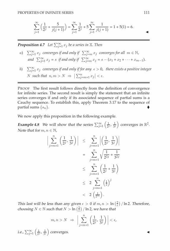
PROPERTIES OF INFINITE SERIES 111
'+
j=1
( 1
2j+
5
j(j + 1)
)=
'+
j=1
1
2j+ 5
'+
j=1
1
j(j + 1)= 1 + 5(1) = 6.
"
Proposition 4.7 Let;'
j=1 xj be a series in X. Then
a);'
j=1 xj converges if and only if;'
j=m xj converges for all m # N,
and;'
j=1 xj = s if and only if;'
j=m xj = s " (x1 + x2 + · · · + xm"1).
b);'
j=1 xj converges if and only if for any ! > 0, there exists a positive integer
N such that n, m > N )
&&;nj=m+1 xj
&& < !.
PROOF The first result follows directly from the definition of convergencefor infinite series. The second result is simply the statement that an infiniteseries converges if and only if its associated sequence of partial sums is aCauchy sequence. To establish this, apply Theorem 3.17 to the sequence ofpartial sums {sn}. #
We now apply this proposition in the following example.
Example 4.8 We will show that the series;'
j=1
(1
2j , 13j
)converges in R2.
Note that for m, n # N,&&&&
n+
j=m+1
21
2j,
1
3j
3 &&&& +
n+
j=m+1
&&&&
21
2j,
1
3j
3&&&&
=n+
j=m+1
'1
22j+
1
32j
+
n+
j=m+1
21
2j+
1
3j
3
+ 2n+
j=m+1
(12
)j
< 2(
12m
).
This last will be less than any given ! > 0 if m, n > ln,
2(
-/ ln 2. Therefore,
choosing N # N such that N > ln,
2(
-/ ln 2, we have that
m, n > N )
&&&&n+
j=m+1
21
2j,
1
3j
3 &&&& < !,
i.e.,;'
j=1
(1
2j , 13j
)converges. "
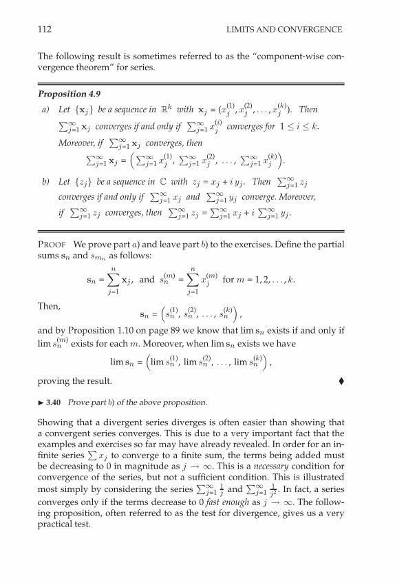
112 LIMITS AND CONVERGENCE
The following result is sometimes referred to as the “component-wise con-vergence theorem” for series.
Proposition 4.9
a) Let {xj} be a sequence in Rk with xj = (x(1)j , x(2)
j , . . . , x(k)j ). Then
;'j=1 xj converges if and only if
;'j=1 x
(i)j converges for 1 + i + k.
Moreover, if;'
j=1 xj converges, then;'
j=1 xj =(;'
j=1 x(1)j ,
;'j=1 x
(2)j , . . . ,
;'j=1 x
(k)j
).
b) Let {zj} be a sequence in C with zj = xj + i yj . Then;'
j=1 zj
converges if and only if;'
j=1 xj and;'
j=1 yj converge. Moreover,
if;'
j=1 zj converges, then;'
j=1 zj =;'
j=1 xj + i;'
j=1 yj .
PROOF We prove part a) and leave part b) to the exercises. Define the partialsums sn and smn as follows:
sn =n+
j=1
xj , and s(m)n =
n+
j=1
x(m)j for m = 1, 2, . . . , k.
Then,sn =
(s
(1)n , s
(2)n , . . . , s
(k)n
),
and by Proposition 1.10 on page 89 we know that lim sn exists if and only if
lim s(m)n exists for each m. Moreover, when lim sn exists we have
lim sn =(
lim s(1)n , lim s
(2)n , . . . , lim s
(k)n
),
proving the result. #
! 3.40 Prove part b) of the above proposition.
Showing that a divergent series diverges is often easier than showing thata convergent series converges. This is due to a very important fact that theexamples and exercises so far may have already revealed. In order for an in-finite series
;xj to converge to a finite sum, the terms being added must
be decreasing to 0 in magnitude as j 3 -. This is a necessary condition forconvergence of the series, but not a sufficient condition. This is illustratedmost simply by considering the series
;'j=1
1j and
;'j=1
1j2 . In fact, a series
converges only if the terms decrease to 0 fast enough as j 3 -. The follow-ing proposition, often referred to as the test for divergence, gives us a verypractical test.

PROPERTIES OF INFINITE SERIES 113
Proposition 4.10 (Test for Divergence)
For {xj} # X, if lim xj $= 0, then;'
j=1 xj is divergent.
A statement that is equivalent to the above proposition is, “If;'
j=1 xj con-verges, then lim xj = 0."
PROOF Assume that;'
j=1 xj converges. For ! > 0, there exists a positiveinteger N such that
m, n > N )
&&&&n+
j=m+1
xj
&&&& < !.
Now, let m = n + 1. Then for n > N , we have&&&&
n+1+
k=n+1
xj
&&&& < !,
i.e.,n + 1 > N ) |xn+1 | < !.
This proves that lim xn+1 = 0, and so lim xn = 0. #
Example 4.11 Consider;'
j=1 xj where xj =(
1j , j+1
j+2
)# R2. Then, since
lim j+1j+2 = 1 $= 0, we have that lim xj $= 0, and so the series must diverge. "
! 3.41 Suppose | xj | ' a rj , where a > 0 and r > 1. Show that
;%j=1 xj diverges.
When a series converges, one can describe more specifically how it converges.The following definition distinguishes between those series that convergeabsolutely and those that converge only conditionally.
Definition 4.12 For a convergent series;'
j=1 xj in X, if the series;'
j=1 |xj |
converges, we say that the series;'
j=1 xj is absolutely convergent. If theseries
;'j=1 |xj | diverges, we say that
;'j=1 xj is conditionally convergent.
Example 4.13 We will show that the series;'
j=1("1)j4(j+1)(2j+1)(2j+3) converges con-
ditionally. To this end, let sn =;n
j=1("1)j4(j+1)(2j+1)(2j+3) . Using partial fractions, it is
easy to see that
sn =n+
j=1
("1)j2
1
2j + 1+
1
2j + 3
3= "
1
3+
("1)n
2n + 3,
and that lim sn = "13 exists. Therefore, the series converges. To show that the
series is not absolutely convergent, consider;'
j=14(j+1)
(2j+1)(2j+3) and its partial
sums given by Hsn =;n
j=14(j+1)
(2j+1)(2j+3) . We estimate the jth term of this partial

114 LIMITS AND CONVERGENCE
sum as follows. Note that when j is large, the numerator “looks like” 4j whilethe denominator “looks like” (2j)(2j) = 4j2, resulting in an overall ratio that“looks like” 1
j . Therefore the “tail” of the series “looks like” the tail of the
divergent harmonic series, and so we suspect we can bound 4(j+1)(2j+1)(2j+3) below
by a harmonic-like term. To this end, we note that 4(j + 1) > 4j for all j ! 1,and (2j + 1) + (2j + j) for all j ! 1. Finally, (2j + 3) + (2j + 3j) for all j ! 1,and so, 4(j + 1)
(2j + 1)(2j + 3)>
4j
(2j + j)(2j + 3j)=
4
15 jfor j ! 1.
From this we see that
Hsn =n+
j=1
4(j + 1)
(2j + 1)(2j + 3)>
4
15
n+
j=1
1
j.
Since the sum on the right-hand side diverges as n 3 -, so too Hsn 3 - as
n 3 -, and the convergence of;'
j=1("1)j4(j+1)(2j+1)(2j+3) is only conditional. "
As the above definition and example indicate, a series that does not convergeabsolutely may still converge conditionally. The following proposition tellsus that absolute convergence of a series implies conditional convergence.
Proposition 4.14 For {xj} # X, if;'
j=1 |xj | converges, then;'
j=1 xj con-verges.
PROOF Let ! > 0 be given. Then, from result b) from Proposition 4.7 onpage 111, there exists an N # N such that
m, n > N )
&&&&n+
j=m+1
|xj |
&&&& < !.
But, &&&&n+
j=m+1
xj
&&&& +n+
j=m+1
|xj | =
&&&&n+
j=m+1
|xj |
&&&& < ! if m, n > N .
Therefore;'
j=1 xj converges, and the result is proved. #
! 3.42 For {xj} ! X such that;%
j=1 |xj | converges, show that
&&&& |x1|&&&&
%+
j=2
xj
&&&&&&& #
&&&&%+
j=1
xj
&&&& #%+
j=1
|xj |.
This is the natural extension of the triangle and reverse triangle inequalities to infiniteseries.
Many results for series, and in particular, many tests for convergence of se-ries, apply only to series in R. We will explore these results and tests in thenext subsection. The significance of the above proposition is that it allows us

PROPERTIES OF INFINITE SERIES 115
to use many of these “R-specific” results and tests even when working witha series in Rk or C. In particular, we can use them to test any series in X forabsolute convergence, since for any xj # X, the quantity |xj | is a real number.
4.3 Special Series
We now describe several special classes of series, each of which occurs fre-quently in practice and has its own convergence and divergence criteria. Westart with one of the most useful classes of infinite series in analysis and inapplications.
Geometric Series
Definition 4.15 An infinite series of the form;'
j=0 rj = 1 + r + r2 + · · · forconstant r # R or C is called a geometric series.
Note from the above that the first summand of a geometric series is 1 by def-inition. Example 4.3 on page 109 is an example of a geometric series. This ispossibly the most important class of series in analysis and will be critical toour development in later chapters. It is also important because of its appear-ance in many applications, as well as the fact that when a geometric seriesconverges, we can determine its sum. The following exercises allow you tocharacterize the convergence properties of geometric series.
! 3.43 Show that, if |r| < 1, the corresponding geometric series converges to the
sum 11!r
. To get started, show that sn = 1!rn+1
1!r.
! 3.44 Show that, if |r| ' 1, the corresponding geometric series diverges.
Alternating Series
An important class of series within R that contains examples that are condi-tionally convergent is the class of alternating series.
Definition 4.16 A series;'
j=1("1)j+1xj with 0 < xj # R for all j is calledan alternating series.
There is an especially convenient test for convergence for alternating series.We establish this test in the following proposition.
Proposition 4.17 (Alternating Series Test)
Suppose;'
j=1("1)j+1xj is an alternating series. If xj ! xj+1 for all j, and iflim xj = 0, then the series converges.

116 LIMITS AND CONVERGENCE
PROOF Let sn =;n
j=1("1)j+1xj . We will show that the odd and even subse-quences, {s2k+1} and {s2k}, both converge to the same limit. To see this, notethat s2k+1 = s2k"1 " x2k + x2k+1 + s2k"1,
and so {s2k+1} is nonincreasing. It is also easy to see that s2k+1 > 0, and so{s2k+1} is bounded below. Therefore, lim s2k+1 = sodd exists. Similarly, we seethat s2k = s2k"2 + x2k"1 " x2k ! s2k"2,
and s2k + x1 for all k (Why?), and so {s2k} is nondecreasing and boundedabove. Therefore, it follows that lim s2k = seven exists. We will now show thatsodd = seven. To establish this, note that s2k+1 = s2k +x2k+1. Taking the limit ask goes to - on both sides of this equality yields the result that sodd = seven.The completion of the proof is left to the reader. #
! 3.45 Complete the proof of the above proposition by showing that for every $ > 0,there exists N " N such that n > N - |sn & s| < $. (Hint: The value of n must beeither even or odd.)
Example 4.18 We will show that the alternating series;'
j=1("1)j 1j is condi-
tionally convergent. (We already know that it is not absolutely convergent.)First, note that
;'j=1("1)j 1
j = ("1);'
j=1("1)j+1 1j , provided the series both
converge. The series on the right converges by the alternating series test,since 1
j > 0 for all j ! 1, and.
1j
/is a decreasing sequence (Why?) with
lim 1j = 0. Therefore, the series
;'j=1("1)j 1
j converges conditionally. "
Series with Nonnegative Terms
The following important results pertain to series whose terms are presumedto be nonnegative real numbers. This is not as restrictive a category as onemight think. It includes situations where one tests a series for absolute con-vergence, even when the series has negative terms, and even when the seriesis a sum of vectors.
Proposition 4.19 Suppose xj ! 0 for all j = 1, 2, . . . . Then;'
j=1 xj converges ifand only if the sequence of associated partial sums {sn} is bounded above.
PROOF Since xj ! 0, it follows that the sequence of partial sums {sn} isincreasing. If {sn} is also bounded above, then lim sn exists, and
;'j=1 xj
converges. Conversely, if;'
j=1 xj converges, then lim sn = s exists, and sothe sequence {sn} must be bounded. #
Example 4.20 We illustrate the use of the above proposition by establishing
the convergence of the series;'
j=0
(12
)j2
. To see this, simply note that for
any integer n ! 0,

PROPERTIES OF INFINITE SERIES 117
sn =n+
j=0
(12
)j2
+
n+
j=0
(12
)j= 2
21 "
(12
)n+13
< 2.
Therefore, according to Proposition 4.19, the series;'
j=0
(12
)j2
converges. "
! 3.46 Give an example of a series from R2 that converges absolutely.
The following test for convergence is of great use in proving theorems. Ofcourse, it can also be used as a practical tool to show that a series converges.
Proposition 4.21 (The Comparison Test)
Suppose 0 + xj + yj for j = 1, 2, . . . . Then the following are true:
a) If;'
j=1 yj converges, then;'
j=1 xj converges, and;'
j=1 xj +
;'j=1 yj .
b) If;'
j=1 xj diverges, then;'
j=1 yj diverges.
PROOF To prove a), let sn =;n
j=1 xj , and tn =;n
j=1 yj be the nth par-tial sums of the two series, and assume that
;'j=1 yj converges. By Propo-
sition 2.2, the sequence of partial sums {tn} is bounded above. Clearly, wehave sn + tn for any n, and so the sequence {sn} is also bounded above. Butsince xj ! 0 for all j, it follows that the sequence {sn} is increasing, and soit must be convergent according to the monotone sequence theorem. It easilyfollows that
;'j=1 xj +
;'j=1 yj . The proof of b) is a direct consequence of part
a), since, according to a) if;'
j=1 yj converges, then;'
j=1 xj converges. Thismeans that the divergence of
;'j=1 xj implies the divergence of
;'j=1 yj . #
! 3.47 Show that the condition “0 # xj # yj for j = 1, 2, . . ." in the comparisontheorem can be weakened to “0 # xj # yj for j ' N for some N " N" and the sameconclusion still holds.
Example 4.22 Consider the series given by;'
j=1
, j2 j+1
-j . Clearly for all j !
1 we have 0 +
, j2 j+1
-j+
,12
-j , where,
12
-j are the terms of a convergent ge-
ometric series. Therefore, by the comparison test,;'
j=1
, j2 j+1
-j converges. "
We now state a particularly potent test for convergence. Its proof relies onthe comparison test.
Theorem 4.23 (The Cauchy Condensation Test)
Suppose {xj} is a nonincreasing sequence, and xj ! 0 for all j. Then the series;'j=1 xj and
;'j=0 2j x2j both converge, or both diverge.
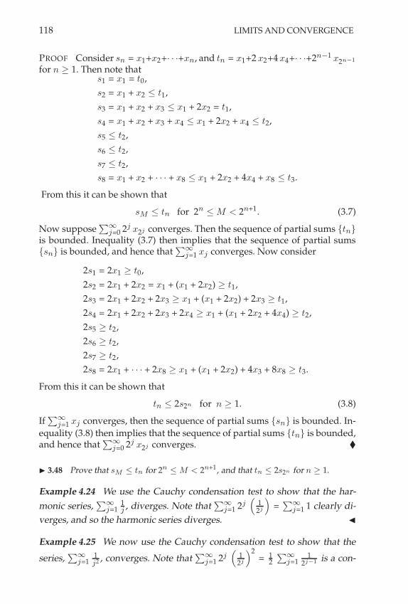
118 LIMITS AND CONVERGENCE
PROOF Consider sn = x1+x2+· · ·+xn, and tn = x1+2 x2+4 x4+· · ·+2n"1 x2n"1
for n ! 1. Then note thats1 = x1 = t0,
s2 = x1 + x2 + t1,
s3 = x1 + x2 + x3 + x1 + 2x2 = t1,
s4 = x1 + x2 + x3 + x4 + x1 + 2x2 + x4 + t2,
s5 + t2,
s6 + t2,
s7 + t2,
s8 = x1 + x2 + · · · + x8 + x1 + 2x2 + 4x4 + x8 + t3.
From this it can be shown that
sM + tn for 2n+ M < 2n+1. (3.7)
Now suppose;'
j=0 2j x2j converges. Then the sequence of partial sums {tn}is bounded. Inequality (3.7) then implies that the sequence of partial sums{sn} is bounded, and hence that
;'j=1 xj converges. Now consider
2s1 = 2x1 ! t0,
2s2 = 2x1 + 2x2 = x1 + (x1 + 2x2) ! t1,
2s3 = 2x1 + 2x2 + 2x3 ! x1 + (x1 + 2x2) + 2x3 ! t1,
2s4 = 2x1 + 2x2 + 2x3 + 2x4 ! x1 + (x1 + 2x2 + 4x4) ! t2,
2s5 ! t2,
2s6 ! t2,
2s7 ! t2,
2s8 = 2x1 + · · · + 2x8 ! x1 + (x1 + 2x2) + 4x3 + 8x8 ! t3.
From this it can be shown that
tn + 2s2n for n ! 1. (3.8)
If;'
j=1 xj converges, then the sequence of partial sums {sn} is bounded. In-equality (3.8) then implies that the sequence of partial sums {tn} is bounded,and hence that
;'j=0 2j x2j converges. #
! 3.48 Prove that sM # tn for 2n # M < 2n+1, and that tn # 2s2n for n ' 1.
Example 4.24 We use the Cauchy condensation test to show that the har-
monic series,;'
j=11j , diverges. Note that
;'j=1 2j
(1
2j
)=
;'j=1 1 clearly di-
verges, and so the harmonic series diverges. "
Example 4.25 We now use the Cauchy condensation test to show that the
series,;'
j=11j2 , converges. Note that
;'j=1 2j
(1
2j
)2= 1
2
;'j=1
12j"1 is a con-

PROPERTIES OF INFINITE SERIES 119
stant multiple of a convergent geometric series, and so the series;'
j=11j2
converges. "
Each of the two previous examples is a member of the more general cate-gory of series known as p-series. Such series have the form
;'j=1
1jp for some
constant real number p. We formally define the p-series below.
Definition 4.26 A series of the form;'
j=11jp for real constant p is called a
p-series.
! 3.49 Show that a given p-series is convergent if and only if p > 1.
While not as useful in proving theorems, the following test is usually moreeasily applied than the comparison test. Its proof, like that of the Cauchycondensation test, relies on the comparison test.
Theorem 4.27 (The Limit Comparison Test)
Suppose;'
j=1 xj and;'
j=1 yj are series of positive terms such that
lim
2xj
yj
3= L > 0 exists.
Then;'
j=1 xj converges if and only if;'
j=1 yj converges.
PROOF There exists an N # N such that
n > N )
&&&&xj
yj" L
&&&& <L
2.
That is,n > N )
1
2L yj < xj <
3
2L yj .
The comparison test now proves the result. #
Example 4.28 We will show that the series;'
j=11
j2"5 j+1converges by use of
the limit comparison test. To find the appropriate candidate for yj to compare
to our xj = 1j2"5 j+1
, we note that to determine the convergence behavior of
a series requires only that we determine the convergence behavior of its tail.That is, how do the terms of the series behave when j is very large? For verylarge j, we see that xj = 1
j2"5 j+1is approximately 1
j2 , and so the natural
choice for yj is yj = 1j2 . Applying the limit comparison test we find
lim
2xj
yj
3= lim
2j2
j2" 5 j + 1
3= lim
I
J 1
1 "5j + 1
j2
K
L = 1.
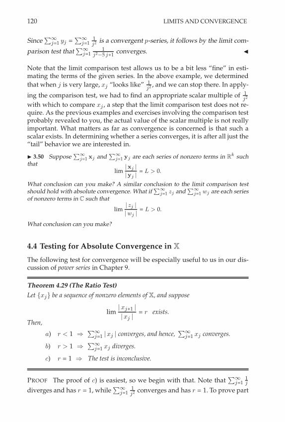
120 LIMITS AND CONVERGENCE
Since;'
j=1 yj =;'
j=11j2 is a convergent p-series, it follows by the limit com-
parison test that;'
j=11
j2"5 j+1converges. "
Note that the limit comparison test allows us to be a bit less “fine” in esti-mating the terms of the given series. In the above example, we determinedthat when j is very large, xj “looks like” 1
j2 , and we can stop there. In apply-
ing the comparison test, we had to find an appropriate scalar multiple of 1j2
with which to compare xj , a step that the limit comparison test does not re-quire. As the previous examples and exercises involving the comparison testprobably revealed to you, the actual value of the scalar multiple is not reallyimportant. What matters as far as convergence is concerned is that such ascalar exists. In determining whether a series converges, it is after all just the“tail” behavior we are interested in.
! 3.50 Suppose;%
j=1 xj and;%
j=1 yj are each series of nonzero terms in Rk such
thatlim
|xj ||yj |
= L > 0.
What conclusion can you make? A similar conclusion to the limit comparison testshould hold with absolute convergence. What if
;%j=1 zj and
;%j=1 wj are each series
of nonzero terms in C such that
lim| zj ||wj |
= L > 0.
What conclusion can you make?
4.4 Testing for Absolute Convergence in X
The following test for convergence will be especially useful to us in our dis-cussion of power series in Chapter 9.
Theorem 4.29 (The Ratio Test)
Let {xj} be a sequence of nonzero elements of X, and suppose
lim|xj+1 |
|xj |= r exists.
Then,
a) r < 1 )
;'j=1 |xj | converges, and hence,
;'j=1 xj converges.
b) r > 1 )
;'j=1 xj diverges.
c) r = 1 ) The test is inconclusive.
PROOF The proof of c) is easiest, so we begin with that. Note that;'
j=11j
diverges and has r = 1, while;'
j=11j2 converges and has r = 1. To prove part

PROPERTIES OF INFINITE SERIES 121
a), note that there exists an N # N such that
j > N )
&&&&|xj+1 |
|xj |" r
&&&& <1 " r
2.
From this we obtain
j > N ) |xj+1 | <
21 + r
2
3|xj |.
Letting t / 1+r2 < 1, this gives
j > N ) |xj+1 | < t |xj |,
which in turn yields
|xj | < tj"N"1|xN+1 | for j ! N + 2.
That is,|xj | <
,t"N"1
|xN+1 |-tj , for j ! N + 2,
and the result follows by use of the comparison test (and Exercise 3.47) wherewe note that the right-hand side of the above inequality represents the jthterm of a convergent geometric series. To prove part b), note that there existsa positive integer N such that for j > N ,
&&&&|xj+1 |
|xj |" r
&&&& <r " 1
2.
This in turn implies that for j > N ,
|xj+1 | >
21 + r
2
3|xj |,
or equivalently, for t / 1+r2 > 1,
|xj | > tj"N"1|xN+1 | for j ! N + 2.
From this it follows that lim xj $= 0. Therefore, by the test for divergence, theseries
;'j=1 xj diverges. #
Example 4.30 Fix z0 # C. We will show that the series;'
n=0zn
0n! converges
absolutely by use of the ratio test. Simply consider the limit
lim
&&&&&zn+1
0 /(n + 1)!
zn0 /n!
&&&&& = lim&&&
z0
n + 1
&&& = 0.
Note that since z0 # C was arbitrary, this result holds for any z0 # C. "
The idea behind the truth of parts a) and b) of the ratio test is that, in eachof these two cases, the tails of the given series can be seen to “look like”that of a convergent or a divergent geometric series, respectively. Since theconvergence behavior of a series depends only on the behavior of its tail, we

122 LIMITS AND CONVERGENCE
obtain a useful test for convergence in these two cases. Case c) is a case thatthe ratio test is not fine enough to resolve. Other methods need to be tried inthis case to properly determine the series” behavior. Similar reasoning givesrise to another useful test that is actually more general than the ratio test,although not always as easy to apply. That test is the root test. Our version ofthe root test defines + as a lim sup rather than as a limit, which gives the testmore general applicability since the lim sup always exists (if we include thepossible value of -), whereas the limit might not. Of course, when the limitdoes exist, it equals the lim sup .
Theorem 4.31 (The Root Test)
Let {xj} be a sequence of nonzero elements of X, and suppose
lim sup j*|xj | = + exists.
Then,
a) + < 1 )
;'j=1 |xj | converges, and hence,
;'j=1 xj converges.
b) + > 1 )
;'j=1 xj diverges.
c) + = 1 ) The test is inconclusive.
PROOF To prove part c), consider;'
j=11j , which diverges, and
;'j=1
1j2 ,
which converges. Both have + = limj('
j%|aj | = 1. Now suppose + < 1. Then
there exists N # N such that
n > N )j*|aj | <
1 + +
2< 1.
From this we haven > N ) |aj | <
(1 + +
2
)j,
and so;'
j=0 |aj | is bounded above by a geometric series and therefore con-verges by the comparison test and Exercise 3.47. Now suppose + > 1. If;'
j=0 aj converges then limj(' aj = 0. Since + = lim sup j%|aj | > 1, there
must be a subsequence of.
j%
|aj |/
that converges to +. But this contradictsthe fact that every subsequence of {aj} must converge to 0, and so
;'j=0 aj
must diverge. #
Example 4.32 Consider the series;'
j=0 aj , where aj is given by
aj =
E,12
-j for odd j ! 1,,
13
-j for even j ! 2.
In this case, even though limj('
j%|aj | does not exist, we do have that
lim sup j*|aj | = 1
2 < 1,

MANIPULATIONS OF SERIES IN R 123
and so by the root test, the series converges. "
Example 4.33 In this example we will see that the root test can work wherethe ratio test fails. Consider the series given by
'+
j=1
e"j+sin (j$/2).
Then aj = e"j+sin (j$/2) and so&&&aj+1
aj
&&& = e"1+sin ((j+1)$/2)"sin (j$/2),
which does not have a limit as j 3 -. Yet,
j*|aj | = e"1+(sin (j$/2))/j ,
which converges to e"1 as j 3 -. Therefore, the series converges by the roottest. "
5 MANIPULATIONS OF SERIES IN R
Several interesting results pertain specifically to the case of series of realnumbers. We discuss these next.
5.1 Rearrangements of Series
We begin with a definition.
Definition 5.1 Let;'
j=1 aj be an infinite series of real numbers correspond-
ing to the sequence {an}. If {a&n} is a permutation1 of {an}, the infinite series;'j=1 a&j is called a rearrangement of
;'j=1 aj .
It is an interesting fact that if;'
j=1 aj is conditionally convergent, one canfind a rearrangement that converges to any specified real number '. How-ever, if
;'j=1 aj is absolutely convergent we will show that every rearrange-
ment converges to the same value. In order to establish these results we willmake use of the following convenient notation. In particular, we define
a+j /
|aj | + aj
2=
$aj if aj ! 00 if aj < 0
, (3.9)
anda"j /
|aj |" aj
2=
$0 if aj > 0
"aj if aj + 0. (3.10)
1A permutation of an means that the terms are placed in a different order.

124 LIMITS AND CONVERGENCE
Note that a+j ! 0 and a"j ! 0. Also, it is easy to see that aj = a+
j " a"j , and
|aj | = a+j + a"j .
Proposition 5.2 Consider the series;'
j=1 aj and the associated series;'
j=1 a+j
and;'
j=1 a"j with a+j and a"j as defined above.
a) If;'
j=1 aj converges conditionally, then both of the series;'
j=1 a+j and
;'j=1 a"j
diverge.
b) If;'
j=1 aj converges absolutely, then both of the series;'
j=1 a+j and
;'j=1 a"j
converge absolutely.
PROOF We prove part a), and leave part b) to the reader. Suppose;'
j=1 aj
converges conditionally and that;'
j=1 a+j converges. Then we have that
;'j=1 a"j =
;'j=1
(a+j " aj
)converges, and so
;'j=1 |aj | =
;'j=1
(a+j + a"j
)
converges, giving a contradiction. Presuming;'
j=1 a"j converges yields asimilar contradiction. #
! 3.51 Prove part b) of the above proposition. To get started, consider that a+j &a
!j
=
aj , and a+j + a
!j
= |aj |.
The proof of the next result is left to the reader.
Proposition 5.3 Suppose;'
j=1 aj converges conditionally. If Sn and Tn are the
partial sums of;'
j=1 a+j and
;'j=1 a"j , respectively, then lim Sn = lim Tn = -.
! 3.52 Prove the above proposition.
The following result is often surprising at first. Of course, as with many the-orems, the proof should make things clearer.
Theorem 5.4 If;'
j=1 aj converges conditionally, then there exists a rearrange-ment of
;'j=1 aj that converges to any real number '.
PROOF Let ' be an arbitrary real number, and let Sn =;n
j=1 a+j and Tn =
;nj=1 a"j . Here, a+
j and a"j are as defined in equations (3.9) and (3.10) on
page 123. The strategy is to add together just enough of the a+j terms to ex-
ceed ', then to subtract just enough of the a"j terms to make the sum no
greater than ', then add more a+j terms to just exceed ' again, and so on,
thereby “zeroing in” on '. To this end, we recall that lim Sn = -, so thereexists n1 ! 1 such that
Sn1 > ' while S) + ' for " < n1.

MANIPULATIONS OF SERIES IN R 125
Similarly, since lim Tn = -, we can find k1 ! 1 such that
Sn1 " Tk1< ' while Sn1 " T) ! ' for " < k1.
Continuing in this way, we can find n2 ! 1 such that
Sn1+n2 " Tk1> ' while Sn1+n2"1 " Tk1
+ ',
and k2 ! 1 such that
Sn1+n2 " Tk1+k2< ' while Sn1+n2 " Tk1+k2"1 ! '.
After such an nj and kj have been found, we have that
Sn1+···+nj " Tk1+···+kj< ' while Sn1+···+nj " Tk1+···+kj"1 ! ',
and therefore,
' + Sn1+···+nj " Tk1+···+kj"1 = Sn1+···+nj " Tk1+···+kj+ a"kj
< ' + a"kj.
That is, &&&Sn1+···+nj " Tk1+···+kj"1 " '&&& < a"kj
,
and since limj(' a"kj= 0 (Why?), it follows that
limj('
(Sn1+···+nj " Tk1+···+kj"1
)= '.
#
! 3.53 Answer the (Why?) question in the above proof.
The following result is often convenient.
Theorem 5.5 If;'
j=1 aj converges absolutely, then every rearrangement of;'
j=1 aj
converges to the same value.
PROOF Let;'
j=1 a&j be a rearrangement of;'
j=1 aj . We will first assume thataj ! 0 for all j. Then, defining Sn / a1 + · · · + an, we have that lim Sn = Sfor some real number S. Define Tn / a&1 + · · · + a&n. Then Tn + S (Why?),and since Tn is bounded above, it follows that lim Tn = T exists and T + S.Similarly, Sn + T (Why?), and so S + T . Therefore, we must have T = S. Thecase where aj < 0 for at least one j is left to the reader. #
! 3.54 Answer the two (Why?) questions in the above proof, and prove the abovetheorem in the case where aj < 0 for at least one j.
5.2 Multiplication of Series
If;'
j=1 aj and;'
j=1 bj are convergent infinite series, it might seem natural
to consider their product,;'
j=1 aj
-,;'j=1 bj
-. How might one define such a
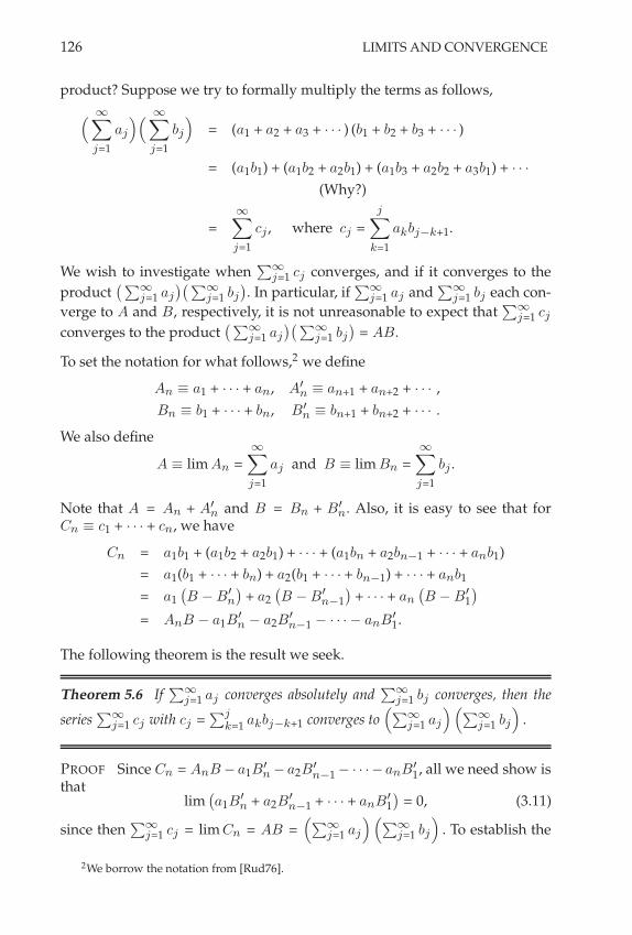
126 LIMITS AND CONVERGENCE
product? Suppose we try to formally multiply the terms as follows,
( '+
j=1
aj
)( '+
j=1
bj
)= (a1 + a2 + a3 + · · · ) (b1 + b2 + b3 + · · · )
= (a1b1) + (a1b2 + a2b1) + (a1b3 + a2b2 + a3b1) + · · ·
(Why?)
='+
j=1
cj , where cj =j+
k=1
akbj"k+1.
We wish to investigate when;'
j=1 cj converges, and if it converges to the
product,;'
j=1 aj
-,;'j=1 bj
-. In particular, if
;'j=1 aj and
;'j=1 bj each con-
verge to A and B, respectively, it is not unreasonable to expect that;'
j=1 cj
converges to the product,;'
j=1 aj
-,;'j=1 bj
-= AB.
To set the notation for what follows,2 we define
An / a1 + · · · + an, A&n / an+1 + an+2 + · · · ,
Bn / b1 + · · · + bn, B&n / bn+1 + bn+2 + · · · .
We also define
A / lim An ='+
j=1
aj and B / lim Bn ='+
j=1
bj .
Note that A = An + A&n and B = Bn + B&
n. Also, it is easy to see that forCn / c1 + · · · + cn, we have
Cn = a1b1 + (a1b2 + a2b1) + · · · + (a1bn + a2bn"1 + · · · + anb1)
= a1(b1 + · · · + bn) + a2(b1 + · · · + bn"1) + · · · + anb1
= a1,B " B&
n
-+ a2
,B " B&
n"1
-+ · · · + an
,B " B&
1
-
= AnB " a1B&n " a2B
&n"1 " · · ·" anB&
1.
The following theorem is the result we seek.
Theorem 5.6 If;'
j=1 aj converges absolutely and;'
j=1 bj converges, then the
series;'
j=1 cj with cj =;j
k=1 akbj"k+1 converges to(;'
j=1 aj
)(;'j=1 bj
).
PROOF Since Cn = AnB " a1B&n " a2B
&n"1 " · · ·" anB&
1, all we need show isthat
lim,a1B
&n + a2B
&n"1 + · · · + anB&
1
-= 0, (3.11)
since then;'
j=1 cj = lim Cn = AB =(;'
j=1 aj
)(;'j=1 bj
). To establish the
2We borrow the notation from [Rud76].

MANIPULATIONS OF SERIES IN R 127
limit (3.11), note that lim B&n = 0 (Why?), and so for any ! > 0 there exists an
N # N such that n > N ) |B&n| < !. That is, there exists an N # N such
that m > 0 ) |B&N+m| < !. We now consider the following estimate:
|a1B&n + a2B
&n"1 + · · · + anB&
1| + |a1||B&n| + |a2||B
&n"1| + · · · + |an||B
&1|
=(|an||B
&1| + · · · + |an"(N"1)||B
&N |
)
+(|an"N ||B&
N+1| + · · · + |a1| |B&n|
)
<(|an||B
&1| + · · · + |an"(N"1)||B
&N |
)
+!
'+
j=1
|aj |. (Why?)
Since lim an = 0, we have for all ! > 0,
lim sup |a1B&n + a2B
&n"1 + · · · + anB&
1| + lim sup
M(|an||B
&1| + · · ·
+ |an"(N"1)||B&N |
)+ !
'+
j=1
|aj |
N
= !
'+
j=1
|aj |. (Why?)
Since this is true for all ! > 0, we have that
lim sup |a1B&n + a2B
&n"1 + · · · + anB&
1| = 0.
Clearly,lim inf |a1B
&n + a2B
&n"1 + · · · + anB&
1| = 0, (Why?)
and thereforelim |a1B
&n + · · · + anB&
1| = 0.
This establishes the limit (3.11), and the theorem is proved. #
! 3.55 Answer the four (Why?) questions from the proof of the previous theorem.
Example 5.7 Recall from Example 4.30 that;'
j=0z
j0
j! converges absolutelyfor any z0 # C. Fix z0 and w0 in C. We will show that
2 '+
j=0
zj0
j!
32 '+
j=0
wj0
j!
3=
'+
j=0
(z0 + w0)j
j!.
To see this, note that by Theorem 5.6 we may write
2 '+
j=0
zj0
j!
32 '+
j=0
wj0
j!
3=
'+
j=0
cj ,

128 LIMITS AND CONVERGENCE
where
cj =j+
m=0
zm0
m!
wj"m0
(j " m)!.
Simple algebra and use of the binomial theorem gives
cj =1
j!
j+
m=0
2j
m
3zm
0 wj"m0 =
1
j!(z0 + w0)j .
"
5.3 Definition of ex for x # R
In this subsection, we formally define the real number denoted by ex for anyfixed x # R. We do this in terms of a convergent series.
Definition 5.8 For any fixed x # R, the real number denoted by ex is definedas
ex/
'+
j=0
xj
j!.
To establish that this series converges absolutely for every x # R, refer toExample 4.30 on page 121. Several familiar properties of ex are a direct con-sequence of the above definition. In particular, note that the number e is nowdefined to be e =
;'j=0
1j! = 1 + 1 + 1
2! + 13! + · · · , a convergent sum. Also,
e0 = 1. While we will assume the reader is familiar with the other propertiesassociated with ex, several of them are available to the reader to establish inthe supplementary exercises at the end of the chapter.
6 SUPPLEMENTARY EXERCISES
1. Suppose the sequence {xn} converges to x " X with the usual norm | · |. We willshow that convergence in X is “norm-independent.” To see this, consider anothernorm | · |1 on X and recall as stated in an earlier exercise that all norms on X areequivalent. That is, there exists " > 0 such that
1"|x|1 # |x| # " |x|1
for every x " X. From this, show that for any $ > 0, there exists an integer N > 0such that n > N - |x & xn|1 < $.
2. Show that lim n3!2 n+122 n4!12
= 0.
3. Does the sequence! (
n2+n+1
n2!n+1 cos n#
3 , n2+n+1
n2!n+1 sin n#
3
) "in R
2 converge? (It does
not. Prove this.)

SUPPLEMENTARY EXERCISES 129
4. If it exists, determine the limit of the sequence {zn} ! C given by zn = n
2n+1 +i (&1)n. If it doesn’t exist, show why not.
5. Suppose {xn} and {yn} are sequences in X such that lim(xn ± yn) = L exists.
a) If lim xn = x exists, what can you say about lim yn? Show that the limit exists, andevaluate it.
b) If lim xn does not exist, what can you say about lim yn? Try finding an examplewhere lim xn and lim yn do not exist but lim(xn + yn) does.
6. Come up with another example of a convergent sequence where the strict inequal-ity < must be replaced by # when taking the limit.
7. Find lim 4n2+1
n3+nby using the squeeze theorem.
8. Use the result of Example 2.7 to determine the limit in Example 2.13.
9. Show that lim n3+n!53n2+1 = / and that lim 1!n
2
1+3n= &/.
10. Show that lim xn = &/ if and only if lim(&xn) = /.
11. Suppose {xn} and {yn} are sequences in X such that lim(xn ± yn) = L exists. Iflim xn = /, what can you say about lim yn? (You should find that the limit is either±/, depending on the various cases.)
12. Suppose the sequence {xn} " R2 is given by xn =
((!1)n
n2 , 4 + sin,
n #
2
-). Find
expressions for the terms of the subsequences {x2m} and {x2m+1}.
13. In the previous exercise, determine whether lim x2m or lim x4m exists. Based onyour conclusions, what do you think is true of lim xn? (You should conclude {xn}does not converge.)
14. Suppose {xn} is a decreasing sequence of positive real numbers. If lim x2m = 1,find lim xn.
15. Does the sequence in Example 3.5 on page 98 have any other limit points? (Yes.)
16. Consider the sequence {zn} " C with zn = 1n
+ i cos,
n #
4
-. Find the limit points
of {zn}.
17. If {xn} in X has exactly one limit point, must {xn} converge? (No. Find a coun-terexample.)
18. Is it true that if the sequence {xn} ! S ! X converges to the limit x, then x mustbe a limit point of S? (Yes. Find a quick proof.)
19. Give an example of a sequence {zn} ! C that does not have a limit point.
20. Let {xn} ! S ! X be a sequence where S is closed. Prove that every limit pointof {xn} lies in S.

130 LIMITS AND CONVERGENCE
21. Find " and + for the real sequence {xn} given by
a) xn = (!1)n n
n+1 b) xn = 1en + cos
,n #
4
-c) xn = 1
n+ sin
,n #
2
-
22. Suppose {xn} and {yn} are bounded sequences of nonnegative real numbers.Show that lim sup(xnyn) #
,lim sup xn
- ,lim sup yn
-.
23. Suppose {yn} is a bounded sequence of real numbers such that lim sup yn = 0.Also suppose that for all $ > 0, there exists N " N such that n > N - |xn| # yn +$.
a) Does lim yn exist? (Yes.) b) Does lim xn exist? (Yes.)
24. In the previous exercise, if the condition on lim sup yn is changed to lim sup yn =" %= 0, what happens to your conclusions in parts a) and b)? (Neither is true anymore.)
25. Show that the sequence {xn} " R2 given by xn =
((12
)n
, n
n+1
)is Cauchy.
26. Find the sum of the series given by;%
j=11
j (j+2) .
27. Show that the series;%
j=11j2 converges. (Hint: First show by induction that sn #
2n
n+1 for all n ' 1.)
28. Use the comparison test to show that the real series given by;%
j=11
j2!5 j+1 con-verges.
29. Suppose xj = (&1)j and yj = (&1)j+1. What can you say about;%
j=1(xj + yj )?What can you say about
;%j=1 xj +
;%j=1 yj? Prove that one series converges, but the
other does not.
30. Suppose the sequences {xj} and {yj} in X are such that;%
j=1(xj + yj ) converges.What can you say about
;%j=1 xj and
;%j=1 yj? What if
;%j=1(xj &yj ) also converges?
In the final case, show that;%
j=1 xj and;%
j=1 yj converge as well; this is not neces-sarily true without that assumption.
31. Show that the series;%
j=1
(#
6 + i
4
)j
converges in C.
32. In Example 4.8 on page 111 we confirmed the convergence of a series in R2.
Determine the sum.
33. Show that the series;%
j=51
2j converges. To what number does this series con-verge?
34. Determine the limit as n goes to / of the product*
' 4*
' 8*
' · · · 2n*
'.
35. Consider the series given by;%
j=0 zj , where zj =(
12j + i
3j
)" C for j = 1, 2, . . . .
Show that the series converges and find the sum.

SUPPLEMENTARY EXERCISES 131
36. Consider the series in C given by;%
j=0
, 1+i
2
-j. Determine whether it converges,
and if so, the sum.
37. Show that the real series given by;%
j=1j
ej converges by using the comparisontest.
38. Consider the series given by;%
j=21
j ln j. How does this series compare to a p-
series? Use the Cauchy condensation test to determine whether it converges. (It doesnot converge.)
39. Show that the real series given by;%
j=1j
ej and by;%
j=11
j (j+1) are convergent byusing the limit comparison test.
40. Using the ratio test, show that r = 1 for the series;%
j=11j
and;%
j=11j2 .
41. In the application of the ratio test, suppose the limit condition is replaced by thefollowing:
r = lim sup|xj+1 ||xj |
exists.
Show that if r < 1 the series converges, while if |xj+1||xj| ' 1 for j ' N for some N " N,
the series diverges.
42. Using the root test, show that , = 1 for the series;%
j=11j
and;%
j=11j2 .
43. Abel’s identity. Suppose {an} is a sequence in R or C, and {bn} is a sequence in X.Let the sequence {Tn} in X be such that Tn & Tn!1 = bn. Show that for n ' m + 2,
n+
j=m+1
aj bj = an Tn & am+1 Tm &n!1+
j=m+1
(aj+1 & aj ) Tj .
Does this result remind you of integration by parts?
44. Abel’s test. Suppose {an} is a sequence in R or C, and {bn} is a sequence in X suchthat
(i);%
j=1 bj converges,
(ii);%
j=2 |aj & aj!1| converges.
Then,;%
j=1 aj bj converges. To show this, define the following four quantities:
K . max
I
J%+
j=2
|aj & aj!1|, |a1|
K
L , B .%+
j=1
bj , Bn .n+
j=1
bj , Tn . Bn & B.
For now, assume that K > 0. Clearly Tn+1 & Tn = bn. Since lim Tn = 0, we know thatfor any $ > 0 there exists N " N such that
n > N - |Tn| <$
6K.
Note thatan = a1 +
n+
j=2
(aj & aj!1),

132 LIMITS AND CONVERGENCE
and so it follows that
|an| # |a1| +n+
j=2
|aj & aj!1| # K + K = 2K for all n.
To determine the convergence of;%
j=1 aj bj we will show that the partial sums areCauchy. To this end, let m < n, and consider that
&&&&&
n+
m+1
aj bj
&&&&& =
&&&&&anTn & am+1Tm &n!1+
m+2
(aj+1 & aj ) Tj
&&&&&
# |an| |Tn| + |am+1| |Tm| +n!1+
m+2
|aj+1 & aj | |Tj |
# 2K
($
6K
)+ 2K
($
6K
)+ K
($
6K
)
< $ whenever m, n > N .
a) What if K = 0 in the above argument? Show that it is a trivial case.
b) What if {an} is a sequence in Rk? Does Abel’s test still apply in some form?
(It does, if {bn} is a sequence in R.)
45. Prove the following corollary to Abel’s test. Suppose {an} is a sequence in R orC, and {bn} is a sequence in X such that
(i);%
j=1 bj converges,
(ii) {an} is monotone and converges.
Then,;%
j=1 aj bj converges.
46. Dirichlet’s test. Suppose {bn} is a sequence in X such that the sequence of partialsums {Bn} given by Bn =
;n
j=1 bj is bounded. Show that if {an} is a sequence in R
or C such that lim an = 0 and;%
j=2 |aj & aj!1| converges, then;%
j=1 aj bj converges.
47. Show that the alternating series test is a special case of Dirichlet’s test.
48. For a sequence {xn} " R, suppose lim xn = x exists. Prove that lim 3*
xn = 3*
x.(Hint: Use the fact that a
3 & b3 = (a & b)(a2 + ab + b
2) for any a, b " R, and considerthe cases x > 0, x < 0, and x = 0 separately.) Can you generalize this result to showthat lim m
*xn = m
*x for any m " N? How about generalizing the result to show that
lim(xn)q = xq for any q " Q?
49. Suppose 0 < x1 < y1, and that xn+1 =*
xnyn and yn+1 = 12 (xn + yn) for n " N.
a) Show that 0 < xn < yn for all n. b) Show that xn < xn+1 for all n.
c) Show that yn+1 < yn for all n. d) Show that lim xn = lim yn = L.
50. Is it possible that lim an = 0 and a);%
j=1aj
jdiverges? (Yes. Find an example.)
b);%
j=1aj
j2 diverges? (No. Prove this.)
51. Is it possible that;%
j=1 aj converges and;%
j=1 a2j diverges? (No. Why?)

SUPPLEMENTARY EXERCISES 133
52. Determine whether the series;%
j=1(!1)j sin j"
jdiverges, converges conditionally,
or converges absolutely.
53. Suppose {yj} is a nonnegative sequence, and that;%
j=1 yj has bounded partialsums. Also, suppose the sequence of real numbers {xn} is such that xn > 0 for all n,and lim xn = 0. Show that
;%j=1 xjyj converges.
54. Let an, for n ' 0 be a sequence of real numbers such that a = lim an exists. Define-n . a0+a1+···+an
n+1 . Prove that lim -n = a. To do so, fix $ > 0, and split in two the sumin the definition of -n at $n. Then take n very large.
55. Suppose {an}, {bn} are real sequences for n ' 1. Suppose further that;%
n=1 an2
and;%
n=1 bn2 converge. Then it can be shown that
;%n=1 anbn converges absolutely
and satisfies&&&&
%+
n=1
anbn
&&&& #
OPPQ%+
n=1
an2
OPPQ%+
n=1
bn2.
a) Does this look familiar for finite sums? You may wish to look back at Chapter 1here where we discussed inner product spaces. Assume the an and bn are nonneg-ative to start with.
b) Prove that the inequality for finite sums can be extended to infinite sums.
56. Prove the following facts relating to ex:
a) exey = e
x+y for all x, y " R. b) e!x = 1
ex for all x " R.c) e
x> 0 for all x " R. d) e
x> x for all x " R.
e) x > 0 - ex
> 1. f) x < 0 - ex
< 1.g) e
x = 1 2 x = 0. h) x < y - ex
< ey for all x, y " R.
i) (ex)n = enx for all n " Z. j) (ex)r = e
rx for all r " Q.
To establish j), begin by showing that (ex)1/n = ex/n for all nonzero n " Z.
57. The Cantor SetRecall the construction of the Cantor set, C, from Exercise 75 on page 80. We will char-acterize points from this set according to their ternary expansion, a concept analagousto a decimal expansion. In fact, for any x " [0, 1] we can write x in decimal expansionform as
x =a1
10+
a2
102+
a3
103+ · · · ,
where each aj " {0, 1, 2, . . . , 9} for j = 1, 2, . . . . This expansion is unique for somex " [0, 1]. For others, there might be more than one decimal expansion representation.
a) Show that for x = 13 , we can write
13
=310
+3
102+
3
103+ · · · ,
and that this representation is unique.
b) Show that for x = 12 , we can write x in a decimal expansion in two ways. (In fact,
any x with a decimal expansion that terminates in an infinite string of ajs equalto 0 can also be written to terminate with an infinite string of 9s as well, and vice

134 LIMITS AND CONVERGENCE
versa.)
c) Show that for x " [0, 1], we can write x in a ternary expansion so that
x =c1
3+
c2
32+
c3
33+ · · · ,
where each cj " {0, 1, 2} for j = 1, 2, . . . . Show that the number x = 13 has two
ternary expansions. (In fact, any x with a ternary expansion that terminates in aninfinite string of cjs equal to 0 can also be written to terminate with an infinitestring of 2s as well, and vice-versa.)
d) Recall from Exercise 75 on page 80 that the construction of the Cantor set C =>%j=0 Cj involves generating a sequence {Cj} of sets starting with the interval C0 =
[0, 1] in R and removing the open middle-third segment G1 =(
13 , 2
3
)to form
C1, removing the two open middle-third segments comprising G2 =(
132 , 2
32
)0
(732 , 8
32
)from C1 to form C2, and so on. The set Gn in this process is the union of
“open middle-thirds” that is removed from Cn!1 to form Cn. Show that if x " G1then c1 = 1, if x " G2 then c2 = 1, and more generally, if x " Gn then cn = 1. Fromthis, conclude that x /" C if and only if cn = 1 for some n. That is, x " C if and onlyif x has a ternary expansion such that cj %= 1 for all j. From this, can you determinethe cardinality of the Cantor set (i.e., how many points are in the Cantor set)?
e) From the results of parts c) and d), you should conclude that x = 13 is in C. In fact,
x = 13 is a boundary point of G1, the first removed middle-third from the Cantor
set construction algorithm. Define K1 .#
(Gj . Can you show that any x " K1 isa Cantor set point? How many such points are there?
f) In fact, C = K1 0 K2 where K2 ! [0, 1], K1 $ K2 = !, and K2 %= !. To prove thislast fact, show that x = 1
4 is in C, but 14 /" K1. How many points must exist in the
set K2?
g) Are there any irrational numbers in C? (Yes.)
h) Can you show that K1 is dense in C? That is, can you show that K1 = C?
i) From the result in part h), show that for any Cantor set point x, there exists asequence of Cantor set points {xj} ! K1 such that lim xj = x.
j) Show that for any Cantor set point x, there exists an increasing sequence of Cantorset points {xj} ! K1 such that lim xj = x. Similarly, show that there exists adecreasing sequence of Cantor set points {xj} ! K1 such that lim xj = x.

4FUNCTIONS: DEFINITIONS AND LIMITS
Mathematics may be defined as the subject in which we never know what we aretalking about, nor whether what we are saying is true.
Bertrand Russell
Much of the material of this chapter should be familiar to students who havecompleted a “transition course” to higher mathematics, and for this reasonmany of the proofs are omitted. We define the general concept of a func-tion and we assume the reader is well acquainted with real-valued func-tions of a single real variable, and even somewhat familiar with real-valuedand vector-valued functions of a vector. We introduce the important classof complex functions in a bit more detail, spending extra effort to investi-gate the properties of some fundamental examples from this special class.While some of these examples are seemingly natural extensions of their real-function counterparts, we will see that there are some significant differencesbetween the real and complex versions. We also consider functions as map-pings and review some basic terminology for discussing how sets of points inthe function’s domain are mapped to their corresponding image sets in thecodomain. We summarize the rules for combining functions to make newfunctions, and we note the special circumstances under which a given func-tion has an associated inverse function. Finally, we investigate the importantprocess of taking the limit of a function in our various cases of interest, a pro-cess that will be used throughout our remaining development of analysis.
1 DEFINITIONS
Although readers are probably familiar with a variety of functions from pre-vious experience, we take the time now to formally discuss what constitutes afunction in the many contexts we will be exploring. Several examples will fa-miliarize the reader with each case. We begin with a summary of our adoptednotation and the definition for function in the most general case.
135

136 FUNCTIONS: DEFINITIONS AND LIMITS
1.1 Notation and Definitions
We will again use the symbol X in all that follows to represent any of thespaces R, C, or Rk in those situations where the result may apply to anyof those spaces. Related to this, we use the symbol D to denote the genericdomain of a function, where D is to be understood as a nonempty subset ofX. In specific examples or results, we will use the more specific notation D1
when the domain lies in R, D when the domain lies in C, and the notationDk when the domain lies in Rk. In a similar fashion to our use of the symbolsX and D, we use the notation Y to denote the codomain of a function, whereY should be interpreted as a subset (possibly a proper subset!) of any of thespaces R, C, or Rp for integer values p ! 2. Note that we use the letter p todenote the dimension of Rp associated with the symbol Y, since the use ofthe letter k is reserved for the space Rk associated with the symbol X. Also,recall that the norm notation | · | will be used for all of the spaces of interest.Finally, as usual, when results do not apply to all the spaces R, C, Rk, andRp, we will refer to the relevant spaces explicitly.
We now provide some definitions that will be used throughout our discus-sion of functions.
Definition 1.1 Suppose for some nonempty D ' X each element in D can beassociated with a unique element in Y. We make the following definitions.
1. The association, denoted by f , is called a function from D into Y,and we write f : D 3 Y.
2. The set D is called the domain of f , and the set Y is called thecodomain of f .
3. For a particular associated x # D and y # Y we write y = f (x).In this case y is referred to as the image of x under f .
4. The range of f consists of all those elements of Y that areimages of some x # D under f . We denote the range of f by
Rf = {y # Y : y = f (x) for some x # D} .
Note that a function f is actually a set of ordered pairs (x, y) with x # D andy = f (x) # Y. In fact, the function f can be understood to be a subset of theCartesian product D.Y. Note too that the domain D does not have to be theentire space X. We can think of X as the ambient space in which the domain D
resides. Finally, note that in general, the range of a function may be a propersubset of its codomain. We can think of Y as the ambient space in which therange Rf resides. The range of f : D 3 Y is also sometimes denoted by f (D).
In referring to a function, we will often allude to the specific spaces D andY on which it is defined. For example, in the special case where D and Y arespecified as subsets of R we will simply write f : D1
3 R, or even f : I 3 R

DEFINITIONS 137
if the domain is an interval I of real numbers. This case corresponds to thefamiliar situation from calculus, that of a real-valued function of a single realvariable. When D is specified as a subset of Rk and Y as R we will writef : Dk
3 R. This corresponds to the case where f is a real-valued function ofseveral real variables, or a real-valued function of a vector. Such real-valued func-tions will often be denoted more explicitly in either of the following ways,
f (x) or f (x1, . . . , xk).
Here, x denotes the vector (usually considered as a row vector) having com-ponents x1, . . . , xk . In the case where D is specified as a subset of Rk andY is specified as Rp, we will write f : Dk
3 Rp, and we are dealing witha vector-valued function of several real variables, or a vector-valued function of avector. Such functions will be more explicitly denoted by either
f (x) or f (x1, . . . , xk).
Here, the bold f indicates its vector value. We will also consider functionsfrom a subset of C to C. For such functions we write f : D 3 C and referto them as complex functions. This class of functions is associated with someof the most interesting and beautiful results in analysis. Complex functionswill often be denoted as f (z) where z = x + i y # C. Finally, in those caseswhere the domain of a function has not been specified, but only its rule orassociation given, the reader should interpret the domain to be the largest setof allowable values within the appropriate space.
1.2 Complex Functions
The special case of complex-valued functions of a complex variable, hereafterreferred to as complex functions, is of great importance in analysis. Not only iscomplex function theory regarded as one of the most beautiful subjects in allof mathematics, it is also one of the most useful, being routinely employedby mathematicians, physicists, and engineers to solve practical problems. Tomany readers the category of complex functions is entirely new, and so wewill develop it a bit more carefully than the more general description of func-tions already presented.
Definition 1.2 A complex function f : D 3 C with D ' C is an associationthat pairs each complex number z = x + i y # D with a complex numberf (z) = u + i v # C. Here, u and v are real-valued functions of x and y. That is,
f (z) = u(x, y) + i v(x, y).
We refer to u(x, y) as the real part of f (z), and to v(x, y) as the imaginary partof f (z).
As we have already seen, C is different from both R and R2 in significantways. Yet we can rely on our knowledge of these more familiar Euclidean
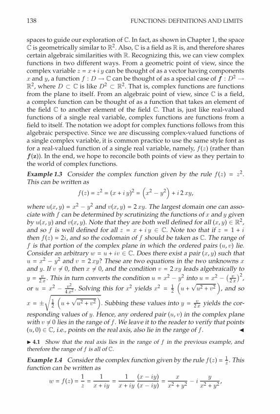
138 FUNCTIONS: DEFINITIONS AND LIMITS
spaces to guide our exploration of C. In fact, as shown in Chapter 1, the spaceC is geometrically similar to R2. Also, C is a field as R is, and therefore sharescertain algebraic similarities with R. Recognizing this, we can view complexfunctions in two different ways. From a geometric point of view, since thecomplex variable z = x+ i y can be thought of as a vector having componentsx and y, a function f : D 3 C can be thought of as a special case of f : D2
3
R2, where D ' C is like D2' R2. That is, complex functions are functions
from the plane to itself. From an algebraic point of view, since C is a field,a complex function can be thought of as a function that takes an element ofthe field C to another element of the field C. That is, just like real-valuedfunctions of a single real variable, complex functions are functions from afield to itself. The notation we adopt for complex functions follows from thisalgebraic perspective. Since we are discussing complex-valued functions ofa single complex variable, it is common practice to use the same style font asfor a real-valued function of a single real variable, namely, f (z) (rather thanf (z)). In the end, we hope to reconcile both points of view as they pertain tothe world of complex functions.
Example 1.3 Consider the complex function given by the rule f (z) = z2.This can be written as
f (z) = z2 = (x + i y)2 =(x2
" y2)
+ i 2 xy,
where u(x, y) = x2" y2 and v(x, y) = 2 xy. The largest domain one can asso-
ciate with f can be determined by scrutinizing the functions of x and y givenby u(x, y) and v(x, y). Note that they are both well defined for all (x, y) # R2,and so f is well defined for all z = x + i y # C. Note too that if z = 1 + ithen f (z) = 2i, and so the codomain of f should be taken as C. The range off is that portion of the complex plane in which the ordered pairs (u, v) lie.Consider an arbitrary w = u + iv # C. Does there exist a pair (x, y) such thatu = x2
" y2 and v = 2 xy? These are two equations in the two unknowns xand y. If v $= 0, then x $= 0, and the condition v = 2 xy leads algebraically to
y = v2 x . This in turn converts the condition u = x2
" y2 into u = x2"
,v
2 x
-2,
or u = x2"
v2
4 x2 . Solving this for x2 yields x2 = 12
(u +
,
u2 + v2)
, and so
x = ±
'12
(u +
,
u2 + v2)
. Subbing these values into y = v2 x yields the cor-
responding values of y. Hence, any ordered pair (u, v) in the complex planewith v $= 0 lies in the range of f . We leave it to the reader to verify that points(u, 0) # C, i.e., points on the real axis, also lie in the range of f . "
! 4.1 Show that the real axis lies in the range of f in the previous example, andtherefore the range of f is all of C.
Example 1.4 Consider the complex function given by the rule f (z) = 1z . This
function can be written as
w = f (z) =1
z=
1
x + iy=
1
x + iy
(x " iy)
(x " iy)=
x
x2 + y2" i
y
x2 + y2,

FUNCTIONS AS MAPPINGS 139
where u(x, y) = xx2+y2 and v(x, y) = "
yx2+y2 . The largest domain one can
associate with f can be determined by scrutinizing the functions of x andy given by u(x, y) and v(x, y), and noting that they are both well definedfor all (x, y) # R2, except (x, y) = (0, 0), and so f is well defined for allz # D = C\{0}. As in the previous example, the codomain can be readily seento be C. To determine the range, first note that for the set of z = (x + i y) # D,the functions u(x, y) = x
x2+y2 and v(x, y) = "y
x2+y2 can each take any real
value, but x and y can never be simultaneously equal to 0. From this we con-clude that the range must exclude w = 0. "
! 4.2 Show that the range of the function in the previous example is, in fact, C \ {0}by considering an arbitrary #+i ) " C\{0} and showing that there exists an x+i y " C
that corresponds to it.
! 4.3 Accomplish the same end as the previous exercise by letting w = f (z) andconsidering z = 1
w. For which complex numbers w does this equation have complex
solutions? Will this technique always work, rather than the lengthier method of theprevious exercise?
2 FUNCTIONS AS MAPPINGS
Sometimes functions are referred to as mappings. The use of the term mappinginstead of function is common when we are discussing sets of points ratherthan an individual point or its image. This point of view stresses the geo-metric nature of a function, viewing it as a transformation that takes a set inthe domain to an image set in the codomain. Within this context, the rangeof a function f : D 3 Y is often denoted by f (D), in which case it can beinterpreted as the image of D under the mapping f . Eventually we will explorewhether certain topological properties of the domain set are retained aftermapping it to the codomain by a particular function. For now, we merely layout the basic ideas associated with thinking of functions as mappings.
2.1 Images and Preimages
Definition 2.1 Consider f : D 3 Y and A ' D. Then the image of A underf is denoted by f (A) and is defined as
f (A) = {y # Y : y = f (x) for some x # A} .
For any set B ' Y, the preimage of B under f is denoted by f"1(B) and isdefined as
f"1(B) = {x # D : f (x) # B} .
The preimage of B under f is sometimes also referred to as the inverse image ofB under f . Note that the notation f"1 here is not meant to denote the inverse

140 FUNCTIONS: DEFINITIONS AND LIMITS
function associated with f . Indeed, such an inverse function may not evenexist. We will review the concept of inverse function a bit later in this chapter.Here, f"1(B) denotes a subset of the domain of f .
We now consider some higher-dimensional examples.
Example 2.2 Suppose f : R23 R2 is given by f (x) = x + a where a # R2 is
a constant vector. Then f is said to “translate” points of R2 a distance |a| inthe direction of a. Let’s apply this function to the set A = {x # R2 : |x " c| =4, where c = (1, 0)} ' R2. Note that A is just the circle of radius 4 centered atthe point c = (1, 0) in R2. From this we have that
f (A) = {y # R2 : y = f (x) for some x # A}
= {y # R2 : y = x + a for x satisfying |x" c| = 4}
= {y # R2 : |(y " a) " c| = 4}
= {y # R2 : |y " (a + c)| = 4}.
This is just the circle of radius 4 centered at a + c in R2. "
Example 2.3 Consider f : C \ {0} 3 C given by f (z) = 1z . We will show that
f maps circles in C \ {0} into circles. Note that, as seen previously,
f (z) =1
z=
x " i y
x2 + y2=
2x
x2 + y2
3" i
2x
x2 + y2
3.
Letting w = u + i v = f (z), we see that
u =x
x2 + y2and v = "
y
x2 + y2,
from which we obtain that
x =u
u2 + v2and y = "
v
u2 + v2.
Now, for z = x + i y and z0 = x0 + i y0, consider the circle of radius r > 0centered at z0 and described by the equation |z " z0| = r. Notice that
|z " z0| = r ) (x " x0)2 + (y " y0)2 = r2.
Subbing our formulas for x and y in terms of u and v into this last equalityobtains ( u
u2 + v2" x0
)2+("
v
u2 + v2" y0
)2= r2.
This, in turn, is equivalent to
(x20 + y2
0 " r2) (u2 + v2) + 2 (y0 v " x0 u) + 1 = 0.
Now, since our original circle of radius r does not pass through the origin,we have that x2
0 + y20 " r2
$= 0, and the above equation can be seen to be theequation of a circle in the variables u and v. "

FUNCTIONS AS MAPPINGS 141
Example 2.4 Let f : C \ {"1} 3 C be given by f (z) = z"1z+1 . We will find the
image of the points on the circle of radius 1 centered at the origin given bythe set A = {z # C \ {"1} : |z| = 1}. Note first that the set A excludes thepoint z = "1, and so is not the whole circle of radius 1 centered at the origin.Then note that
f (z) =z " 1
z + 1=
(x + iy) " 1
(x + iy) + 1=
(x2 + y2" 1) + i2y
(x + 1)2 + y2. (4.1)
Also, since |z| = 1 for each z # A, we have x2 + y2 = 1, and so (4.1) becomes
f (z) = i( y
x + 1
)for z # A. (4.2)
Hence, f has pure imaginary values on the set A. We leave it to the reader toshow that f (A) is the whole imaginary axis. "
! 4.4 Consider the function f and the set A from the previous example. Determinethat f (A) is the whole imaginary axis by using equation (4.2) and considering anarbitrary pure imaginary number i). Show that there exists an x and a y such that) = y
x+1 and x + iy " A.
We now summarize several useful properties regarding images and preim-ages of functions. These results are usually proved in a transition course tohigher mathematics, and so we omit the proof for brevity.
Proposition 2.5 For f : D 3 Y, suppose {A&} ' D, and {B'} ' Y. Then thefollowing all hold.
a) f (%A&) =#
f (A&)
b) f"1,%B'
-=#
f"1(B')
c) f (&A&) '>
f (A&)
d) f"1,&B'
-=>
f"1(B')
Suppose A ' D and B ' Y. Then the following hold.
e) f"1 (f (A)) : A
f) f,f"1(B)
-' B
2.2 Bounded Functions
The following definition specifies a special case where the range is a boundedsubset of the codomain.

142 FUNCTIONS: DEFINITIONS AND LIMITS
Definition 2.6 A function f : D 3 Y is bounded on D if there exists anM # R such that
|f (x)| + M for all x # D.
That is, a function f : D 3 Y is bounded on D if the range of f is a boundedsubset of Y.
Example 2.7 Let f : Rk3 R be given by f (x) = e"|x|2. Then f is bounded
on its domain. To see this, note that since |x| ! 0, it follows that "|x|2 + 0,and therefore
e"|x|2+ e0 = 1 for all x # R
k . "
Example 2.8 Let f : D 3 C be given by f (z) = 1(z+1)2 where D = {z # C :
Re(z) ! 0}. Then, since Re(z) ! 0, it follows that |z + 1| ! 1 (Why?), andtherefore
|f (z)| =1
|z + 1|2+ 1 on D.
Therefore f is bounded on D. "
! 4.5 Answer the (Why?) question in the previous example.
2.3 Combining Functions
The following rules for combining functions should be familiar to the reader.We list them here for completeness. For simplicity in expressing and prop-erly interpreting the statements that follow, the codomain Y should be un-derstood to be the whole space R, C, or Rp, and not a proper subset of any ofthem.
Sums, Differences, and Scalar Multiples of Functions
Suppose f and g are functions from the same domain D to codomain Y. Then,
1. f ± g : D 3 Y are functions, and (f ± g)(x) = f (x) ± g(x) for all x # D.
2. c f : D 3 Y for c # R is a function, and (c f )(x) = c f (x) for all x # D.
Note that the constant c in statement 2 above can also be a complex numberin the case of a complex function f . While the same is true even when f is realvalued, we won’t have need to work with such products in our developmentof analysis.1
1One could also define a complex multiple of a vector-valued function, but the resultingfunction is complex vector valued, a case we don’t consider in our development of analysis.

FUNCTIONS AS MAPPINGS 143
Products and Quotients of Functions
Suppose f : D 3 Yf and g : D 3 Yg are functions from the same domain D.Then,
1. (f · g) : D 3 Yf ·g where (f · g)(x) = f (x) · g(x) for all x # D is a function inthe following cases:
a) Yf = R, Yg = Yf ·g = Y,
b) Yf = Yg = Rp, Yf ·g = R,
c) Yf = Yg = Yf ·g = C,
2. (f/g) : D 3 Yf/g where (f/g)(x) = f (x)/g(x) for all x # D, providedg(x) $= 0 is a function in the following cases:
a) Yf = Y, Yg = R, and Yf/g = Y
b) Yf = Yg = Yf/g = C.
Note that in 1 the product between f and g should be interpreted as the dotproduct when Yf and Yg are both Rp, and as the usual product when Yf andYg are both R or C.
Composition of Functions
We now formally define the composition of functions. In what follows, eachof Yf and Yg should be understood to be any of the spaces R, Rp, or C.
Definition 2.9 Consider f : D 3 Yf with Rf = f (D), and g : Rf 3 Yg .Define the function g ; f : D 3 Yg by
(g ; f )(x) = g (f (x)) for all x # D.
The function g ; f is called the composition of g with f .
Example 2.10 Consider f : R 3 R2 and g : Rf 3 C, where f (x) = (x2, 3 "
x), and g(r, s) = r2 ei s. Then, g ; f : R 3 C, and
(g ; f )(x) = g (f (x)) = g(x2, 3 " x) = x4 ei (3"x).
Note that the domain of g is the range of f given by Rf = {(x, y) # R2 : x !
0}. Also note that f ; g does not exist in this case since f (g(r, s)) = f,r2 ei s
-
is not defined. "
Example 2.11 Consider f : C\{"1}3 C given by f (z) = z+1z"1 . We will write
f as a composition of simpler functions. To this end, note that
f (z) =z + 1
z " 1=
(z " 1) + 2
z " 1= 1 +
2
z " 1. (4.3)

144 FUNCTIONS: DEFINITIONS AND LIMITS
We now define the following:
f1 : C \ {1} 3 C \ {0}, given by f1(z) = z " 1,
f2 : C \ {0} 3 C, given by f2(z) = 2z ,
f3 : C 3 C, given by f3(z) = 1 + z.
Note from this that
f (z) = 1 +2
z " 1= 1 +
2
f1(z)= 1 + f2 (f1(z)) = f3
,f2 (f1(z))
-,
and therefore, f = f3 ; f2 ; f1. "
2.4 One-to-One Functions and Onto Functions
There are properties a function might possess that indicate in significantways what kind of function it is, what operations it will allow, or to what,if any, other functions it might be related. In this subsection, we review twosuch important properties. We begin with a definition.
Definition 2.12 Suppose f : D 3 Y is a function such that for all pairsx, Gx # D, the following property holds,
f (x) = f (Gx) ) x = Gx.
Then we say that f is a one-to-one function, or that f is 1-1.
A statement that is equivalent to the above definition is that a function f :D 3 Y is one-to-one if and only if for x, Gx # D, x $= Gx ) f (x) $= f (Gx). One-to-one functions are those functions that map no more than one element of theirdomains into a given element of their codomains. Another term for one-to-one that is often used in analysis is injective. Such a function is referred to asan injection. Our first example establishes that linear functions are one-to-one.
Example 2.13 Consider f : C 3 C given by f (z) = az + b, where a, b # C,and a $= 0. We will show that f is one-to-one. To see this, let z, Gz # C be suchthat f (z) = f (Gz). Simple algebra obtains z = Gz, and therefore f is one-to-one."
Example 2.14 Consider f : Rk3 R given by f (x) = 1
|x|+1. Let ej for j =
1, . . . , k denote the unit vectors in Rk whose components are all zeros exceptfor the jth component, which has the value 1. Clearly f is not one-to-one,since f (ej) = f (em) for j $= m such that 1 + j, m + k. "
The first result we will establish about one-to-one functions involves a par-ticular type of real-valued function of a single real variable, namely, strictlymonotone functions. We define monotone functions and strictly monotone func-tions next.

FUNCTIONS AS MAPPINGS 145
Definition 2.15 A real-valued function f : D13 R is called monotone if
any of the following hold true. For all x1, x2 # D1,
1. x1 < x2 ) f (x1) + f (x2). In this case, the monotone function is callednondecreasing.
2. x1 < x2 ) f (x1) < f (x2). In this case, the monotone function is calledincreasing.
3. x1 < x2 ) f (x1) ! f (x2). In this case, the monotone function is callednonincreasing.
4. x1 < x2 ) f (x1) > f (x2). In this case, the monotone function is calleddecreasing.
A function f is called strictly monotone if it is either increasing or decreasing.
Since the definition relies on the order property exclusively possessed by thereal numbers, it does not make sense to refer to a monotone function that isnot real-valued or whose domain is not a subset of R. Monotone functions areconvenient functions with which to work, as we will soon see. For example,strictly monotone functions are necessarily one-to-one.2
Proposition 2.16 Suppose f : D13 R is a strictly monotone function. Then f is
one-to-one on D1.
PROOF Suppose f (x1) = f (x2) and that f is decreasing (the increasing caseis handled similarly). If x1 < x2 then f (x1) > f (x2), a contradiction. If x1 > x2
then f (x1) < f (x2), also a contradiction. Therefore we must have x1 = x2, andso f is one-to-one. #
The above proposition allows us a convenient means, in some cases anyway,for establishing that a function is one-to-one. If we can show that the functionis strictly monotone, then it must be one-to-one as well.
! 4.6 Consider D1 ! R and consider fj : D
1 , R for j = 1, 2, . . . , p. Is it true that if
fj is a one-to-one function for j = 1, 2, . . . , p, then the function f : D1 , R
p given byf = (f1, f2, . . . , fp) is one-to-one? (Yes.) How about the converse? (No.)
! 4.7 Consider Dk ! R
k and consider fj : Dk , R for j = 1, 2, . . . , p. Is it true that
if fj is a one-to-one function for j = 1, 2, . . . , p, then the function f : Dk , R
p givenby f (x) = (f1(x), f2(x), . . . , fp(x)) is one-to-one? (Yes.) How about the converse? (No.)
2Note that some texts use the terms increasing and strictly increasing in place of nondecreas-ing and increasing, respectively. Likewise, such texts also use the terms decreasing and strictlydecreasing in place of nonincreasing and decreasing.
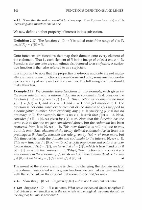
146 FUNCTIONS: DEFINITIONS AND LIMITS
! 4.8 Show that the real exponential function, exp : R , R given by exp(x) = ex is
increasing, and therefore one-to-one.
We now define another property of interest in this subsection.
Definition 2.17 The function f : D 3 Y is called onto if the range of f is Y,i.e., if Rf = f (D) = Y.
Onto functions are functions that map their domain onto every element ofthe codomain. That is, each element of Y is the image of at least one x # D.Functions that are onto are sometimes also referred to as surjective. A surjec-tive function is then also referred to as a surjection.
It is important to note that the properties one-to-one and onto are not mutu-ally exclusive. Some functions are one-to-one and onto, some are just one-to-one, some are just onto, and some are neither. The following example shouldmake this clear.
Example 2.18 We consider three functions in this example, each given bythe same rule but with a different domain or codomain. First, consider thefunction f : R 3 R given by f (x) = x2. This function is not one-to-one sincef ("1) = f (1) = 1, and so x = "1 and x = 1 both get mapped to 1. Thefunction is not onto, since every element of the domain R gets mapped toa nonnegative number. More explicitly, any y # R satisfying y < 0 has nopreimage in R. For example, there is no x # R such that f (x) = "3. Next,consider f : R 3 [0,-) given by f (x) = x2. Note that this function has thesame rule as the one we just considered above, but the codomain has beenrestricted from R to [0,-) ' R. This new function is still not one-to-one,but it is onto. Each element of the newly defined codomain has at least onepreimage in R. Finally, consider the rule given by f (x) = x2 once more, butthis time restrict both the domain and codomain to the interval [0,-) ' R.This new function f : [0,-) 3 [0,-) is both one-to-one and onto. It is one-to-one since, if f (x) = f (Gx), we have that x2 = (Gx)2, which is true if and only if|x| = |Gx|, which in turn means x = Gx. (Why?) The function is onto since if y isany element in the codomain,
,
y exists and is in the domain. That is, for anyy # [0,-) we have y = f (
,
y) with,
y # [0,-). "
The moral of the above example is clear. By changing the domain and/orthe codomain associated with a given function, we can make a new functionwith the same rule as the original that is one-to-one and/or onto.
! 4.9 Show that f : [0, /) , R given by f (x) = x2 is one-to-one, but not onto.
! 4.10 Suppose f : D , Y is not onto. What set is the natural choice to replace Y
that obtains a new function with the same rule as the original, the same domain asthe original, but that is now onto?

FUNCTIONS AS MAPPINGS 147
Of course, as one might expect, functions that are both one-to-one and ontoare special.
Definition 2.19 A function that is both one-to-one and onto is called a one-to-one correspondence.
One-to-one correspondences are important in many areas of mathematics.Such a function may also be referred to as a bijection. The function, possessingboth the one-to-one and the onto properties, is then said to be bijective. Thefollowing example illustrates that linear complex functions are one-to-onecorrespondences.
Example 2.20 Let f : C 3 C be given by f (z) = az + b where a, b # C anda $= 0. We will show that f is onto. To this end, consider an arbitrary w # C.If we can find a z # C such that f (z) = w, i.e., such that az + b = w, we will bedone. But clearly z = w"b
a has the desired property, and so f is onto. "
As learned in typical transition courses to higher mathematics, it is exactlyone-to-one correspondences that have inverses. We review this idea next.
2.5 Inverse Functions
We begin by formally defining the inverse function for a function.
Definition 2.21 Consider the function f : D 3 Rf , where Rf = f (D). Ifthere exists a function g : Rf 3 D such that
(i) f (g(y)) = y for all y # Rf .
(ii) g (f (x)) = x for all x # D,
then g is called the inverse function of f .
A few remarks relating to this definition are in order.
1. Note that if g is the inverse of f , then f is the inverse of g. The pair offunctions, f and g, are called inverse functions, and the inverse of f is oftendenoted by f"1 instead of g.
2. When f"1 exists, f,f"1(y)
-= y for all y # Rf . That is, f ; f"1 = IRf
,
the identity function on Rf . Similarly, f"1 (f (x)) = x for all x # D, i.e.,
f"1; f = ID, the identity function on D.
3. The two identity functions described in the last remark are in general notthe same, since D and Rf are in general not the same.
Example 2.22 Let f : C\{1} 3 C\{1} be given by f (z) = z+1z"1 . The reader is
asked to verify that this function is, in fact, a one-to-one correspondence. We
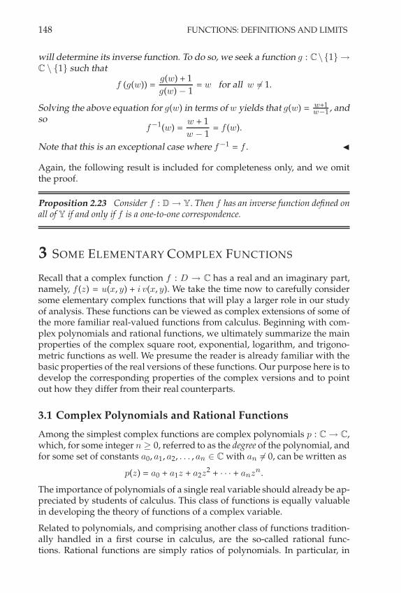
148 FUNCTIONS: DEFINITIONS AND LIMITS
will determine its inverse function. To do so, we seek a function g : C\{1} 3
C \ {1} such that
f (g(w)) =g(w) + 1
g(w) " 1= w for all w $= 1.
Solving the above equation for g(w) in terms of w yields that g(w) = w+1w"1 , and
sof"1(w) =
w + 1
w " 1= f (w).
Note that this is an exceptional case where f"1 = f . "
Again, the following result is included for completeness only, and we omitthe proof.
Proposition 2.23 Consider f : D 3 Y. Then f has an inverse function defined onall of Y if and only if f is a one-to-one correspondence.
3 SOME ELEMENTARY COMPLEX FUNCTIONS
Recall that a complex function f : D 3 C has a real and an imaginary part,namely, f (z) = u(x, y) + i v(x, y). We take the time now to carefully considersome elementary complex functions that will play a larger role in our studyof analysis. These functions can be viewed as complex extensions of some ofthe more familiar real-valued functions from calculus. Beginning with com-plex polynomials and rational functions, we ultimately summarize the mainproperties of the complex square root, exponential, logarithm, and trigono-metric functions as well. We presume the reader is already familiar with thebasic properties of the real versions of these functions. Our purpose here is todevelop the corresponding properties of the complex versions and to pointout how they differ from their real counterparts.
3.1 Complex Polynomials and Rational Functions
Among the simplest complex functions are complex polynomials p : C 3 C,which, for some integer n ! 0, referred to as the degree of the polynomial, andfor some set of constants a0, a1, a2, . . . , an # C with an $= 0, can be written as
p(z) = a0 + a1z + a2z2 + · · · + anzn.
The importance of polynomials of a single real variable should already be ap-preciated by students of calculus. This class of functions is equally valuablein developing the theory of functions of a complex variable.
Related to polynomials, and comprising another class of functions tradition-ally handled in a first course in calculus, are the so-called rational func-tions. Rational functions are simply ratios of polynomials. In particular, in

SOME ELEMENTARY COMPLEX FUNCTIONS 149
the complex case, if p, q : C 3 C are complex polynomials, then the function
r : D 3 C given by r(z) = p(z)q(z) is a complex rational function, where D ' C
is the set of complex numbers that excludes the zeros of the polynomial q.
An example of such a rational function is given by r(z) = z3+z+7z4"z2 defined on
D ' C with D = C \ {"1, 0, 1}.
3.2 The Complex Square Root Function
Recall from Chapter 1 that every z # C \ {0} can be written in polar form asz = r ei " , where r = |z| and $ is an angle measured counterclockwise from thepositive real axis to the ray in the complex plane emanating from the originthrough z. We called $ an argument of z, denoted it by arg z, and noted that $is not unique since
z = r ei " = r ei ("+2 $ k) for k # Z.
This means there are infinitely many ways to represent any particular z # C\
{0} in polar form. Restricting $ = arg z to the interval ("%, % ] distinguisheda unique choice of argument for z and defined a function of z that we calledthe principal branch of the argument and denoted by Arg(z) or !. The key pointhere is that Arg(z) is a function while the unrestricted arg z is not. In fact,Arg(z) is a function from C \ {0} to R. Recall also that f (x) =
,
x was madeinto a function by requiring the symbol
,
x to represent only the nonnegativesquare root of x. Can something similar be done in C where x is replaced byz # C? Yes! We will use the Arg function to define a square root function inC. To this end, consider g : C \ {0} 3 C given by
g(z) = z12 =
(r ei!
)1/2= r
12 ei 1
2 !.
Note that 0 has been excluded from the domain of g because the argument ofz = 0 is not well defined. We can, however, “patch” our function g at z = 0.We do this in the following definition.
Definition 3.1 Let z = r ei!# C, where r = |z| and ! = Arg(z). Then the
complex square root function f : C 3 C is defined as
f (z) =
Er
12 ei 1
2 ! for z $= 00 for z = 0
.
Note that,f (z)
-2 =,r
12 ei 1
2 !-2 = r ei ! = z for z $= 0, and
,f (0)
-2 = 02 = 0,
which implies (f (z))2 = z for all z # C. Therefore the function h : C 3 C
given by h(z) = z2 is a function that takes our defined square root of z backto z.
! 4.11 Show that the square root function f : C , C given in Definition 3.1 is one-

150 FUNCTIONS: DEFINITIONS AND LIMITS
to-one. Is it onto? (No.) What can you conclude about the function h : C , C given
by h(z) = z2? Is it f
!1? (No.)
Two well-known properties of the real square root function f : [0,-) 3 R
given by f (x) =,
x are
(i) f (x1x2) = f (x1)f (x2),
(ii) f(
x1x2
)= f (x1)
f (x2) , provided x2 $= 0.
However, these familiar properties do not hold for the complex square rootfunction given in Definition 3.1. We establish this for (i) and leave (ii) to thereader. Let z1 = "1 " i and z2 = "i. Then
f (z1) = 21/4 ei 5$/8, and f (z2) = ei 3$/4.
But z1z2 = "1 + i, and so
f (z1z2) = 21/4 ei 3$/8, while f (z1)f (z2) = 21/4 ei 11$/8.
! 4.12 Find a pair of complex numbers z1, z2 that violates property (ii) above. Whyexactly do properties (i) and (ii) fail to hold for the complex square root function?
! 4.13 Note that for the real square root function f : [0, /) , R given by f (x) =*
x,we know that f (x2) = |x| = x. Now consider the complex square root function givenby Definition 3.1. It is still true that f (z2) = z, but f (z2) %= |z|. Why is that?
3.3 The Complex Exponential Function
Consider the complex function given by the rule f (z) = ez. Recall that thusfar we have defined ei "
/ cos $ + i sin $ for $ # R. This formula definesexponentials for pure imaginary numbers i $. We would now like to extendthis definition to handle exponentials of more general complex numbers z =x + i y.
Definition 3.2 Let z = x + i y # C. Then the function exp : C 3 C given byexp(z), or more commonly denoted by ez, is defined by
exp(z) = ez/ ex ei y.
The motivation for this definition should be clear. We are merely extendingthe traditional rules of manipulating exponents for real numbers as learnedin calculus. Note that this definition is consistent with our notion of expo-nentiation of pure imaginary numbers (corresponding to x = 0), as it mustbe. Note too, however, that the complex exponential function differs fromthe real exponential function in significant ways. For instance, the complexexponential function is not one-to-one, since
exp(z + 2 % i) = ez+2 $ i = ez e2 $ i = ez = exp(z)

SOME ELEMENTARY COMPLEX FUNCTIONS 151
for every z # C, and so exp is periodic with period 2%i. Also, exp(i%) =cos % + i sin % = "1, and so the complex exponential function takes negativereal values.
We now consider some important algebraic properties of ez . We state themin the form of a proposition.
Proposition 3.3 Let z, z1, and z2 be in C. Then
a) ez1+z2 = ez1ez2 ,
b) e"z = (ez)"1,
c) |ez| = eRe(z),
d) ez1 = ez2 if and only if z2 = z1 + i 2% k for some k # Z,
e) ez$= 0.
PROOF Properties a) and b) are simple consequences of the definition. Theseand property e) are left to the exercises. To prove c), we take norms to obtain
|ez| =
&&&ex ei y&&& = |ex
|
&&&ei y&&& = |ex
| = ex.
To establish property d), we equate (after application of the definition)
ex1 ei y1 = ex2 ei y2 ,
which implies that ex1 = ex2 . (Why?) From this it follows that x1 = x2. Wealso have that ei y1 = ei y2 , which implies that y2 = y1 + 2% k for some integerk. Overall this gives
z2 = x2 + i y2 = x1 + i (y1 + 2% k) = z1 + 2% i k for some k # Z.
We have shown that ez1 = ez2 ) z2 = z1 + i 2% k for some integer k. Theconverse follows readily from Definition 3.2. #
! 4.14 Prove properties a), b), and e) of the above proposition.
! 4.15 Show that the range of the complex exponential function is C \ {0}.
! 4.16 Show that the following properties hold for the complex exponential func-tion: a) e
z1!z2 = ez1
ez2 b) e0 = 1 c) (ez)n = e
nz for all n " Z.
More general powers of complex numbers will be postponed until we define the com-plex logarithm function.
3.4 The Complex Logarithm
In what follows we will denote the natural logarithm of a general complexnumber by “log” and reserve the calculus notation “ln” for those cases where

152 FUNCTIONS: DEFINITIONS AND LIMITS
we are taking the natural logarithm of a positive real number.3 In defining acomplex logarithm function, we would like to preserve the inverse relation-ship between the logarithm and the exponential as learned in calculus, andso in our definition of the log of a complex number z we require that
elog z = z.
Certainly this will preserve the relevant inverse relationship in the specialcase when z is real and positive. Also note that since ew
$= 0 for any w # C,we immediately see that the logarithm of 0 will remain undefined, even inthe complex case. With these ideas in mind, consider z = r ei "
$= 0 and letw = log z = & + i -, where here & and - are real numbers. It then followsthat ew = e#+i * . But ew = elog z = z = r ei " as well, and so we have thate#+i * = r ei ". From this we obtain
e#+i* = r ei " = eln rei " = eln r+i ".
(Note our use of ln in this last expression, since it is known that r is a positivereal value.) From this last equality we may conclude that
& + i - = ln r + i $ + i 2% k for some k # Z.
Equating the real and imaginary parts obtains
& = ln r and - = $ + 2% k for k # Z.
Overall, we see that a nonzero complex number z = r ei" has infinitely manylogarithms given by
log z = ln r + i ($ + 2% k) for k # Z.
Again we point out that the ln r appearing on the right side of the aboveequality is the “ordinary,” single-valued natural logarithm of a positive realnumber as encountered in calculus, while log z is the newly defined, multiple-valued natural logarithm of a complex number.
We now consider a few examples to illustrate how to compute logarithms inthe context of complex numbers. To do so, it is often easiest to first convertthe given z to its most general polar form.
Example 3.4 We will find the natural logarithm of the following:
a) z = i b) z = 1 + i c) z = "1 d) z = 1
In all that follows, k should be understood to be an arbitrary integer value.
a) Here, z = i = ei (!2
+2$ k). Taking the logarithm gives
log i = ln 1 + i,
$2 + 2% k
-= i
,$2 + 2% k
-.
3This is not necessarily standard notation. The notation log is typically used for either con-text described here, at least in higher mathematics. For most mathematics students, in fact, thenotation ln is rarely encountered after a first-year calculus course, and rarely is any base otherthan e ever used in analysis. For these reasons, there is never really any confusion as to whichbase is implied by either notation. Our reasons for distinguishing between the two situationswill become clear shortly.

SOME ELEMENTARY COMPLEX FUNCTIONS 153
b) z = 1 + i =,
2 ei (!4 +2$ k). Taking the logarithm gives
log (1 + i) = ln,
2 + i,
$4 + 2% k
-.
c) z = "1 = ei($+2$ k). Taking the logarithm gives
log ("1) = ln 1 + i (% + 2% k) = i (% + 2% k).
d) z = 1 = ei (0+2$ k). Taking the logarithm gives
log 1 = ln 1 + i (0 + 2% k) = i 2% k. "
Note from this example that our new, generalized definition of natural loga-rithm allows us to take the logarithm of negative real numbers. This wasn’tpossible with the old logarithm from calculus. Note also that with the newlydefined logarithm, any nonzero real number (in fact, any nonzero complexnumber too) has infinitely many logarithms instead of just one. This last factmeans that our complex logarithm, as defined so far, is not yet a function.
We now state the relationship between the complex logarithm and the com-plex exponential in the form of a proposition.
Proposition 3.5
a) For nonzero z # C, elog z = z.
b) For any z # C, log ez = z + i 2%k for k # Z.
PROOF To prove a), note that log z = ln |z| + i ($ + 2% k), so exponentiatinggives
elog z = eln |z|+i ("+2$ k) = eln |z|ei ("+2$ k) = |z| ei " = z.
To establish b), note that ez = ex ei y , and so taking logarithms gives
log ez = log(ex ei y
)= ln ex + i (y + 2% k) = (x + i y) + i 2% k = z + i 2% k. #
As explained prior to the statement of the above proposition, just as for com-plex square roots, if z $= 0 # C the complex quantity log z has infinitely manypossible values. We will once again use the principal branch of the argument,Arg, to define a single-valued function from our complex logarithm.
Definition 3.6 Let z = r ei"$= 0 be a complex number. Then if ! = Arg(z) is
the principal branch of the argument of z, we define the principal branch ofthe complex logarithm function Log : C \ {0} 3 C by
Log(z) / ln r + i Arg(z) = ln r + i !.
Note that other “branches” of the complex logarithm can be defined as func-tions as well. This is done by restricting arg z to intervals of length 2 % other

154 FUNCTIONS: DEFINITIONS AND LIMITS
than ("%, % ]. The principal branch is distinguished from other possible defi-nitions of single-valued complex logarithm functions by its designation Log(z)rather than log(z).
! 4.17 Determine the range of the complex logarithm function, Log : C \ {0} , C.(Hint: Consider its real and imaginary parts.)
! 4.18 Show that the complex logarithm function Log : C \ {0} , C is one-to-one.
! 4.19 Proposition 3.5 established that elog z = z and that log e
z = z+i 2 ' k for k " Z
for all nonzero z " C. What can you say about eLog(z) and Log (ez)? (The latter need
not equal z.)
3.5 Complex Trigonometric Functions
We have already seen in Chapter 1 that
sin $ =ei "
" e"i "
2 i, and cos $ =
ei " + e"i "
2.
We would like any generalization of these formulas with the real value $replaced by the more general complex number z to reduce to the above in thespecial case where z is real. To this end, we make the following definition.
Definition 3.7 For z # C define the complex functions sin : C 3 C andcos : C 3 C by
sin z /
ei z" e"i z
2 i, and cos z /
ei z + e"i z
2.
! 4.20 Find Re(sin z), Im(sin z), Re(cos z), and Im(cos z).
We illustrate the use of Definition 3.7 to calculate some complex trigonomet-ric values in the following examples.
Example 3.8 In this example, we will determine cos (i) and sin (1 + i). Ap-plying the definitions, we have
cos (i) =ei i + e"i i
2=
e"1 + e
2, a real number.
Similarly, we find that
sin (1 + i) =ei (1+i)
" e"i (1+i)
2 i=
eie"1" e"ie
2 i.
But ei = cos(1) + i sin (1), and e"i = cos (1) " i sin (1). Overall then, we have
sin (1 + i) =
2e"1 + e
2
3sin (1) " i
2e"1
" e
2
3cos (1).
"

SOME ELEMENTARY COMPLEX FUNCTIONS 155
We now consider the properties of the complex trigonometric functions todetermine how they might differ from their real function counterparts. Tothis end, consider the function sin : C 3 C as defined in Definition 3.7. Therange is the set R =
.w # C : w = (ei z
" e"i z)/(2 i) for some z # C/
. Wewill show that R = C. To prove this, we must solve the equation w = (ei z
"
e"i z)/(2 i) for z. Multiplying this equation by 2 i, by ei z , and rearranging,yields the quadratic equation in ei z given by
(ei z
)2" 2 i w
(ei z
)" 1 = 0.
Solving for ei z via the quadratic formula obtains ei z = i w ±
,
1 " w2. Fromthis we get
z =1
ilog
(i w ±
%1 " w2
).
For any choice of w # C this formula provides a z # C (in fact, infinitelymany) as a preimage of w, and so R = C. Therefore, sin z is unbounded, avery different situation from the case of real-valued trigonometric functions.This unboundedness property can also be established as follows:
&& sin z&& =
&&&&ei z
" e"i z
2 i
&&&&
=1
2
&&&ei (x+i y)" e"i (x+i y)
&&&
=1
2
&&&ei x e"y" e"i x ey
&&&
!
1
2
,ey
" e"y-
,
from which it follows that sin z is unbounded on C. (Why?)
! 4.21 Answer the (Why?) question above. Also, show that the complex functioncos z has range C, and is therefore unbounded on C.
! 4.22 Establish the following properties of the complex sine and cosine functions.Note that each one is a complex analog to a well-known property of the real sine andcosine functions.
a) sin(&z) = & sin z b) cos(&z) = cos z c) sin2z + cos2
z = 1
d) sin(2 z) = 2 sin z cos z e) sin(z + 2 ') = sin z f ) cos(z + 2 ') = cos z
g) sin(z + ') = & sin z h) cos(z + ') = & cos z i) cos(2 z) = cos2z & sin2
z
j) sin,z + #
2
-= cos z
! 4.23 Show that sin(z1 + z2) = sin z1 cos z2 + cos z1 sin z2 and that cos(z1 + z2) =cos z1 cos z2 & sin z1 sin z2.
! 4.24 Show that ei z = cos z + i sin z for any z " C.

156 FUNCTIONS: DEFINITIONS AND LIMITS
4 LIMITS OF FUNCTIONS
Consider a function f : D 3 Y, and suppose x0 # D&, the derived set ofD. Since there exist points x # D arbitrarily close to x0, we can consider thevalues f (x) as x gets closer and closer to x0. In particular, if we let x get arbi-trarily close to x0, does f (x) get arbitrarily close to an element in Y? In orderto consider such a limit as well defined, we require that f (x) get arbitrarilyclose to the same element in Y no matter how we let x approach x0. We for-malize these ideas in defining the limit of a function, a concept that is crucialto the development of analysis.
4.1 Definition and Examples
We begin with a definition.
Definition 4.1 Suppose f : D 3 Y is a function and x0 # D&. We say thelimit of f (x) as x # D approaches x0 exists and equals L, and we write
limx(x0
f (x) = L,
if for each ! > 0 there exists a . > 0 such that
x # D and 0 < |x " x0| < . ) |f (x) " L| < !.
Several remarks are worth noting about this definition.
1. The point x0 must be in D&, since it is only such points that can be ap-proached arbitrarily closely by points x # D.
2. The limit limx(x0 f (x) may exist even if f is not defined at x0. That is, thelimit point x0 might not be in the domain of f .
3. In general, . will depend on ! and x0.
4. The value of . is not unique, since any .& < . will also work.
5. Even in cases where both f (x0) and limx(x0 f (x) exist, they may not beequal to each other.
6. In those cases where Y is a proper subset of R, Rp, or C, it is possible forthe limit L to be in Y but not in Y.
7. An alternative, equivalent notation for the condition “x # D and 0 <|x " x0| < ." that is sometimes used is “x # D & N &
+(x0)."
8. The limit process described here is not the same as that associated with alimit of a sequence as defined in the last chapter. Here, x is not constrainedto approach x0 via a particular sequence of values {xn} within the domainof f . The limit process described here is one that implicitly applies for anysequence {xn} converging to x0, and for which xn $= x0 for each xn. Of

LIMITS OF FUNCTIONS 157
course, in those cases where one knows that the limit according to Defi-nition 4.1 exists, one can take the limit along a particular sequence. Thatis, suppose f : D 3 Y is a function where x0 is a limit point of D. Iflimx(x0 f (x) = L, and if {xn} is a sequence in D such that xn $= x0 for alln and limn(' xn = x0, then limn(' f (xn) = L.
! 4.25 Prove the statement at the end of remark 8 above. That is, for a functionf : D , Y and x0 a limit point of D, suppose limx&x0 f (x) = L. If {xn} is a sequencein D such that xn %= x0 for all n and limn&% xn = x0, then limn&% f (xn) = L. Whatif the sequence does not satisfy the condition that xn %= x0 for all n? (In that case, theresult fails.)
! 4.26 Consider f : R2 \ {0} , R given by
f (x, y) =x y
x2 + y2for any (x, y) " R
2 \ {0}.
Show that the limit lim(x,y)&(0,0) f (x, y) does not exist. (Hint: Argue by contradiction,using the result of remark 8 above.)
We now provide several examples to illustrate the use of Definition 4.1 inestablishing the limit of a function.
Example 4.2 For f : R 3 R given by f (x) = x2, we will show that limx(3 f (x) =9. Note that
|x2" 9| = |x " 3| |x + 3| = |x " 3| |(x " 3) + 6| + |x " 3|2 + 6 |x " 3|.
For arbitrary ! > 0, if we force |x " 3|2 < (2 , i.e., |x " 3| <
%(2 , and also
6 |x " 3| < (2 , i.e., |x " 3| < (
12 , then we obtain |x2" 9| < ! as desired. Taking
. = min,%
(2 , (
12
-, we have that x satisfying 0 < |x"3| < . ) |x2
"9| < !."
Example 4.3 For f : C \ {"1, 1} 3 C given by f (z) = z2+1z2"1
, we will showthat limz(0 f (z) = "1. Let ! > 0 be given, and note that
&&&&z2 + 1
z2" 1
+ 1
&&&& =2 |z|2
|z2" 1|
.
Suppose 0 < |z| < 12 . Then |z2
" 1| ! 1 " |z|2 > 34 , so that
&&&&z2 + 1
z2" 1
+ 1
&&&& =2 |z|2
|z2" 1|
<8
3|z|2.
This last expression will be less than ! as long as |z| <*
3 (8 . We therefore
choose . / min
212 ,*
3 (8
3, and we have
0 < |z| < . )
&&&&z2 + 1
z2" 1
+ 1
&&&& < !."
Note that in the two previous examples, limx(x0 f (x) = f (x0). This is notalways the case.

158 FUNCTIONS: DEFINITIONS AND LIMITS
Example 4.4 Consider f : R 3 R given by f (x) =
$3x + 1 for x $= 2
1 for x = 2.
We will show that limx(2 f (x) = 7. Note that for x $= 2, i.e., for 0 < |x " 2|,we have that |f (x) " 7| = |(3x + 1)" 7| = 3 |x" 2|. This last expression will beless than any arbitrary ! > 0 if |x " 2| < (
3 . That is, letting . = (3 obtains
0 < |x " 2| < . ) |f (x) " 7| = 3 |x " 2| < !. "
Note in the last example that f (2) is defined, and limx(2 f (x) exists, butlimx(2 f (x) $= f (2).
Example 4.5 Consider f : R 3 R given by f (x) = sin x. We will establishthat limx(0 sin x = 0. To see this, let 0 < ! < 1 and choose . < sin"1 !. Then,
0 < |x| < . ) | sin x " 0| = | sin x| < sin . < !. "
! 4.27 Show that lim%&0 cos % = 1. To do this, draw the unit circle and consider theray with angle % having small magnitude as measured from the positive x-axis. Recallthat cos % corresponds to the x coordinate of the point of intersection of this ray withthe unit circle. Use the definition of limit along with the geometry of the problemto derive the conclusion. That is, for $ > 0 find . > 0 such that 0 < |%| < . -| cos % & 1| < $.
In the following example we show how to confirm that a proposed limitingvalue for a function is not the correct limit.
Example 4.6 For f : R 3 R given by f (x) = x2" 2 we will show that
limx(0 f (x) $= "1. To this end, assume that limx(0 f (x) = "1. We will obtaina contradiction. Assuming the limit, let ! = 1
2 . Then there exists a . > 0 suchthat
0 < |x| < . )
&&&x2" 2 + 1
&&& < 12 .
This in turn yields that
0 < |x| < . )
&&&x2" 1
&&& < 12 .
But by the triangle inequality we have that 1 " x2+
&&x2" 1
&& < 12 , i.e.,
0 < |x| < . ) |x| > 1$2
.
This is clearly a contradiction, since whenever |x| is close enough to 0 it can-not simultaneously be greater than 1$
2. Therefore limx(0 f (x) $= "1. "
Finally, in the following examples, we illustrate the case where the argumentof the function approaches a limit point that is not in the function’s domain.
Example 4.7 Consider f : R \ {0} 3 R given by f (x) = x3"2xx . Note that
x = 0 is not in the domain of f , and hence, f (0) is not defined. We will showthat limx(0 f (x) = "2. To this end, let ! > 0 be arbitrary and consider
|f (x) " ("2)| =
&&&&x3
" 2x
x+ 2
&&&& =
&&&&x3
x
&&&& = x2 if x $= 0.

LIMITS OF FUNCTIONS 159
Since x2 < ! as long as |x| <,
!, it follows that taking . =,
! yields
0 < |x| < . ) |f (x) " ("2)| < !. "
! 4.28 Show that the real function f : R \ {0} , R given by f (x) = exp,& 1/x
2-
has a limit of 0 as x , 0, but that the complex function f : C \ {0} , C given byf (z) = exp
,& 1/z
2- does not have a limit as z , 0.
We now consider a higher-dimensional example.
Example 4.8 Consider f : R2\ {0} 3 R2 given by
f (x) =
Cx2
1
|x|,
x22
|x|
D
for any x = (x1, x2) # R2.
We will show that limx(0 f (x) = 0. As in the previous example, note thatthe point x = 0 is not in the domain of f , and hence f (0) is not defined.However, since x = 0 is a limit point of the domain of f we may consider thelimit limx(0 f (x). To this end, note that for x $= 0,
|f (x) " 0| =
&&&&&
Cx2
1
|x|,
x22
|x|
D&&&&& =1
|x|
*x4
1 + x42
+
x21 + x2
2
|x|
= |x|.
Therefore, taking . = ! yields
0 < |x " 0| < . ) |f (x) " 0| < !,
and the limit is established. "
Example 4.9 Consider f : R2\ {0} 3 R given by
f (x, y) =x y
x2 + y2,
and consider the limit lim(x,y)((0,0) f (x, y). In order for the limit to exist, thesame limiting value must be obtained regardless of the path of approach(x, y) takes toward (0, 0). We will show that the limit does not exist. To doso, we will investigate the limit along straight lines passing through the ori-gin. Let y = m x for some fixed m # R and note that along this line,
lim(x,y)((0,0)
f (x, y) = limx(0
m x2
x2 + m2x2= lim
x(0
m
1 + m2,
a value that clearly depends on the slope of the line of approach of (x, y)toward (0, 0). Therefore, the limit does not exist. "
The last example illustrates a significant difference between establishing alimit for a function of more than one real variable and establishing a limit for

160 FUNCTIONS: DEFINITIONS AND LIMITS
a function of a single real variable. In the latter case, the limit exists as longas the same value is obtained as x approaches its limit point from either theleft or the right (these two limits are referred to as left-hand and right-handlimits, respectively, and will be discussed later in this chapter). When thefunction depends on two or more variables, there are an infinite number ofways to approach the limit point. Since one can’t exhaust all possible paths(even checking all possible straight line paths is not sufficient), the definitionis often the only way to establish the limit for such functions, when it exists.
4.2 Properties of Limits of Functions
In this subsection, we discuss some properties of limits of functions that ei-ther allow for easier computation of the limits, or that imply certain nicecharacteristics about the functions in question if the limits exist. We’ll beginwith a result that proves the uniqueness of the limit, when it exists.
Proposition 4.10 For f : D 3 Y and x0 # D&, suppose limx(x0 f (x) exists.Then the limit is unique.
PROOF Suppose limx(x0 f (x) = A and limx(x0 f (x) = B. Then, for any! > 0 there exist .1 > 0 and .2 > 0 such that
x # D and 0 < |x " x0| < .1 ) |f (x) " A| <!
2,
and
x # D and 0 < |x " x0| < .2 ) |f (x) " B| <!
2.
Choosing . < min (.1, .2), if x # D is such that 0 < |x " x0| < . we have
|A " B| = |A " f (x) + f (x) " B| + |A " f (x)| + |f (x) " B| < !.
Since this is true for arbitrary ! > 0, it follows that A = B. Therefore the limitis unique. #
When we learn that the limit of a function limx(x0 f (x) exists we have actu-ally learned more about the function than merely the value of the limit itself.When such a limit exists, the function cannot behave too wildly near thatlimit point. That is, the behavior of the function is constrained to a certaindegree in the immediate vicinity of the limit point x0. In fact, the next resultestablishes that such a function must be bounded near that limit point.
Proposition 4.11 Consider f : D 3 Y and suppose x0 # D&. If limx(x0 f (x) =A exists, then there exists a deleted neighborhood N &
+(x0) centered at x0 such that fis bounded on N &
+(x0) & D.

LIMITS OF FUNCTIONS 161
PROOF According to Definition 4.1 there exists a . > 0 such that for x # D
and 0 < |x"x0| < ., i.e., for x # N &+(x0)&D, we have |f (x)"A| < 1. Applying
the triangle inequality, we easily obtain for all such x that
|f (x)| = |f (x) " A + A| + |f (x) " A| + |A| < 1 + |A|.
This proves the result. #
Example 4.12 Recall that in Example 4.7 on page 158 we showed the the
function f : R \ {0} 3 R given by f (x) = x3"2xx has the limit limx(0 f (x) =
"2. We now will show that f is bounded on N &1(0). To see this, consider an
arbitrary x # N &1(0). Then 0 < |x| < 1, and so we have
|f (x)| =
&&&&x3
" 2x
x
&&&& =&&&x2
" 2&&& + |x|2 + 2 < 3.
"
The following useful result might be called “the component-wise limit theo-rem.” To make its usefulness even more plain, note that for any f : Dk
3 Rp
we may write f (x) in terms of its component functions fj : Dk3 R for
1 + j + p. That is, f (x) =,f1(x), f2(x), . . . , fp(x)
-. Similarly, for any complex
function f : D 3 C where z = x + i y # D, we have f (z) = u(x, y) + i v(x, y)with u(x, y) and v(x, y) considered as “component functions” of f (z). The fol-lowing result summarizes the idea.
Proposition 4.13
a) Consider f : Dk3 Rp where f (x) =
,f1(x), f2(x), . . . , fp(x)
-for each
x # Dk , and let x0 be a limit point of Dk . Then,
limx(x0
f (x) = A with A =,A1, A2, . . . , Ap
-# R
p
if and only if limx(x0fj(x) = Aj for each 1 + j + p.
b) Consider the complex function f : D 3 C where f (z) = u(x, y) + i v(x, y)
for each z = x + i y # D, and let z0 = x0 + i y0 be a limit point of D.
Then,lim
z(z0f (z) = u0 + i v0 # C
if and only if lim(x,y)((x0,y0) u(x, y) = u0 and lim(x,y)((x0,y0) v(x, y) = v0.
PROOF We prove a) and leave the proof of b) to the reader. Supposelimx(x0
f (x) = A. Then, for each ! > 0 there exists a . > 0 such that
0 < |x " x0| < . ) |f (x) " A| < !. (4.4)
But &&fj(x) " Aj
&& + |f (x) " A| for each 1 + j + p,
and so expression (4.4) implies
0 < |x " x0| < . )
&&fj(x) " Aj
&& < ! for each 1 + j + p.
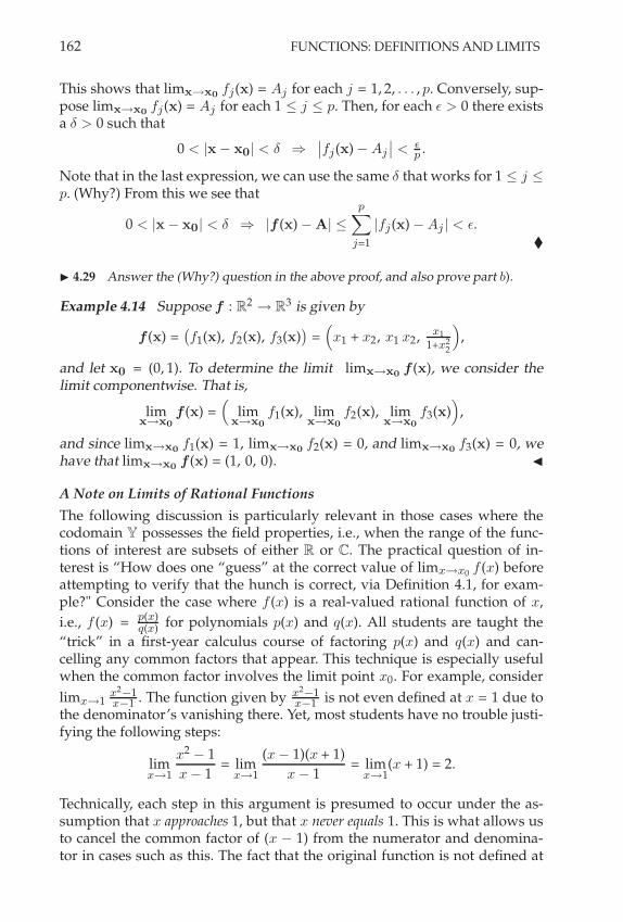
162 FUNCTIONS: DEFINITIONS AND LIMITS
This shows that limx(x0fj(x) = Aj for each j = 1, 2, . . . , p. Conversely, sup-
pose limx(x0fj(x) = Aj for each 1 + j + p. Then, for each ! > 0 there exists
a . > 0 such that
0 < |x " x0| < . )
&&fj(x) " Aj
&& < (p .
Note that in the last expression, we can use the same . that works for 1 + j +
p. (Why?) From this we see that
0 < |x " x0| < . ) |f (x) " A| +
p+
j=1
|fj(x) " Aj | < !.#
! 4.29 Answer the (Why?) question in the above proof, and also prove part b).
Example 4.14 Suppose f : R23 R3 is given by
f (x) =,f1(x), f2(x), f3(x)
-=(x1 + x2, x1 x2, x1
1+x22
),
and let x0 = (0, 1). To determine the limit limx(x0f (x), we consider the
limit componentwise. That is,
limx(x0
f (x) =(
limx(x0
f1(x), limx(x0
f2(x), limx(x0
f3(x))
,
and since limx(x0f1(x) = 1, limx(x0
f2(x) = 0, and limx(x0f3(x) = 0, we
have that limx(x0f (x) = (1, 0, 0). "
A Note on Limits of Rational Functions
The following discussion is particularly relevant in those cases where thecodomain Y possesses the field properties, i.e., when the range of the func-tions of interest are subsets of either R or C. The practical question of in-terest is “How does one “guess” at the correct value of limx(x0 f (x) beforeattempting to verify that the hunch is correct, via Definition 4.1, for exam-ple?" Consider the case where f (x) is a real-valued rational function of x,
i.e., f (x) = p(x)q(x) for polynomials p(x) and q(x). All students are taught the
“trick” in a first-year calculus course of factoring p(x) and q(x) and can-celling any common factors that appear. This technique is especially usefulwhen the common factor involves the limit point x0. For example, consider
limx(1x2"1x"1 . The function given by x2"1
x"1 is not even defined at x = 1 due tothe denominator’s vanishing there. Yet, most students have no trouble justi-fying the following steps:
limx(1
x2" 1
x " 1= lim
x(1
(x " 1)(x + 1)
x " 1= lim
x(1(x + 1) = 2.
Technically, each step in this argument is presumed to occur under the as-sumption that x approaches 1, but that x never equals 1. This is what allows usto cancel the common factor of (x " 1) from the numerator and denomina-tor in cases such as this. The fact that the original function is not defined at

LIMITS OF FUNCTIONS 163
x = 1 does not deter us from readily determining the function’s limit as x
approaches 1. We have really replaced the original function f (x) = x2"1x"1 with
another function g(x) = (x + 1) in this limit calculation. The reason the limitresult for g equals that of the function f is that these functions give the samevalues everywhere in a neighborhood of the limit point x0, except at the limitpoint itself. We formalize this idea in the following result.
Proposition 4.15 Suppose D is a subset of X, and that x0 # D&&DC . Consider f :
D 3 Y and g : D0 3 Y, where D0 = D%{x0}. If f = g on D and limx(x0 g(x) = A,then limx(x0 f (x) = A as well.
PROOF For any ! > 0 there exists a . > 0 such that
x # D0 and 0 < |x " x0| < . ) |g(x) " A| < !.
Since f (x) = g(x) for all x # D, we have that
x # D and 0 < |x " x0| < . ) |f (x) " A| < !,
i.e., limx(x0
f (x) = A.#
! 4.30 If the condition “f = g on D" in the statement of the above result is replacedby “f = g on N
#r(x0) $ D," does the conclusion of the proposition still hold? (Yes.)
Example 4.16 Consider f : R \ {0} 3 R given by
f (x) =x3
" 2 x
x.
Since x3"2 xx = x2
" 2 if x $= 0, let g : R 3 R be given by g(x) = x2" 2.
Since limx(0 g(x) = "2 and f = g on R \ {0}, the previous result allows us toconclude that
limx(0
x3" 2 x
x= lim
x(0(x2
" 2) = "2."
4.3 Algebraic Results for Limits of FunctionsGeneral Results
We now present some limit rules that allow for easy manipulation of limits offunctions. Most of these rules are familiar to students of calculus, and manyof the proofs are left as exercises for the reader. The following proposition isanalogous to Proposition 2.3 of the last chapter, which established a similarset of rules for manipulating limits of sequences.
Proposition 4.17 Consider the functions f and g, both with domain D and codomainY, where Y is here understood to be the whole space R, Rp, or C. Also suppose x0 isa limit point of D. If limx(x0 f (x) = A and limx(x0 g(x) = B, then

164 FUNCTIONS: DEFINITIONS AND LIMITS
a) limx(x0 (f (x) ± y0) = A ± y0 for y0 # Y,
b) limx(x0 (f ± g) (x) = A ± B,
c) limx(x0 (c f ) (x) = c A for c # R or C,
d) limx(x0 (f · g) (x) = A · B,
e) limx(x0 |f (x)| = |A|.
Note that the product in part d) is to be interpreted as the dot product in Rp,and the usual product in R or C.
PROOF We prove b) and d) and leave the other properties to the reader asexercises. To prove b), note that for a given ! > 0, there exists a .1 > 0 suchthat
x # D and 0 < |x " x0| < .1 ) |f (x) " A| <!
2, (4.5)
and also a .2 > 0 such that
x # D and 0 < |x " x0| < .2 ) |g(x) " B| <!
2. (4.6)
For x # D satisfying 0 < |x " x0| < . = min(.1, .2), expressions (4.5) and (4.6)yield
| (f ± g) (x) " (A ± B)| = | (f (x) " A) ± (g(x) " B) |
+ |f (x) " A| + |g(x) " B|
< !.
The proof of d) is similar to the proof of the corresponding property fromProposition 2.3. In particular, note that
|f (x) · g(x) " A · B| = |f (x) · (g(x) " B) + B · (f (x) " A)|
+ |f (x)| |g(x) " B| + |B| |f (x) " A|. (4.7)
The idea is to find an upper bound for each x-dependent term on the right-hand side of inequality (4.7). To this end, note that since limx(x0 f (x) ex-ists there exists a deleted neighborhood N &
r(x0) such that f is bounded onN &
r(x0) & D. That is, |f (x)| + M on N &r(x0) & D for some number M . Now
consider that for ! > 0 there exists .1 > 0 such that x # D satisfying 0 <|x " x0| < .1 yields
|g(x) " B| <!
2(M + 1).
Finally, for ! > 0 there exists .2 > 0 such that x # D satisfying 0 < |x"x0| < .2
yields
|f (x) " A| <!
2(|B| + 1).
Considering only those x # D satifying 0 < |x " x0| < . = min(.1, .2, r), we

LIMITS OF FUNCTIONS 165
can substitute these upper bounds into the original inequality (4.7), yielding
|f (x) · g(x) " A · B| + |f (x)| |g(x) " B| + |B| |f (x) " A|
< M!
2 (M + 1)+ |B|
!
2 (|B| + 1)
=!
2
2M
M + 1
3+
!
2
2|B|
|B| + 1
3
<!
2+
!
2= !.
Since ! was arbitrary, the result is proved. #
! 4.31 Prove the remaining results of the above proposition.
! 4.32 Suppose the functions f and g are such that f : D , Y1 and g : D , Y2where Y1 is either R or C, and Y2 is one of the spaces R, C, or R
p. What can you sayabout property d) from the above proposition? (Similar results should hold.)
A Field Property Result for Limits of Real or Complex Valued Functions
As described in previous chapters, certain results rely explicitly on the prop-erties of a field. As we did in Chapter 3 when discussing sequences of num-bers, we now prove one such result dealing with limits of functions whereone of the functions takes its values in either the real or complex field, R orC. The reader is urged to compare the following proposition with Proposi-tion 2.4 on page 93 of the above referenced chapter.
Proposition 4.18 Consider two functions f and g, both having domain D. Assumef has codomain Y and that g has codomain R or C. (If its codomain is C, then weassume that of f is C too to avoid complex vectors.) Suppose also that x0 # D&. Then,if limx(x0 g(x) = B $= 0, and if limx(x0 f (x) = A, we have that
limx(x0
2f
g
3(x) =
A
B.
Note that if Y = Rk and g has codomain R, then the division in the statementof the theorem is legitimate: one is dividing a vector by a scalar, or multiply-ing the former by the inverse of the latter. Also, that scalar is nonzero in asmall deleted neighborhood of x0 since B $= 0, as we shall see in the proof.
PROOF Consider the case f / 1 on D. To prove the result, note that&&&&
1
g(x)"
1
B
&&&& =|g(x) " B|
|B| |g(x)|.
Since B $= 0 there exists a .1 > 0 such that x # D satisfying 0 < |x " x0| < .1
implies |g(x) " B| <|B|
2 . This in turn implies, for x # D satisfying 0 < |x "
x0| < .1, that |g(x)| >|B|
2 . (Why?) In particular, g(x) $= 0 for such x. Finally,

166 FUNCTIONS: DEFINITIONS AND LIMITS
for ! > 0 there exists a .2 > 0 such that x # D satisfying 0 < |x " x0| < .2
yields |g(x) " B| <( |B|2
2 . From all this, we see that for . = min (.1, .2) andx # D & N &
+(x0), we obtain&&&&
1
g(x)"
1
B
&&&& =|g(x) " B|
|B| |g(x)|< !.
We leave the general case to the reader. #
! 4.33 Complete the proof of the proposition by handling the case where f %. 1.
! 4.34 If p(z) = c0 + c1 z + c2 z2 + · · · + cn z
n with cj " R or C for 1 # j # n, showthat limz&z0 p(z) = p(z0).
! 4.35 Consider f : D , C where f (z) = p(z)q(z) , and p(z) and q(z) are polynomials
in z. Let D = C \ Zq where Zq is the set of roots of the polynomial q. Show that
limz&z0 f (z) = p(z0)q(z0) as long as z0 " D.
Order Property Results for Real-Valued Functions
Finally, as we did for sequences of real numbers in Chapter 3, we now con-sider those special rules relating to the order property of R. In particular, forreal-valued functions f the following proposition is analogous to Proposi-tion 2.5 on page 93 and its corollary from section 2.2.
Proposition 4.19 Consider f and g where both are functions from D to codomainR. Suppose x0 is a limit point of D, and that limx(x0 f (x) = A and limx(x0 g(x) =B. a) If f (x) ! 0 on N &
+(x0) & D for some . > 0, then A ! 0.
b) If f (x) ! g(x) on N &+(x0) & D for some . > 0, then A ! B.
PROOF To prove a), suppose A < 0. Then there exists a .1 > 0 such that
x # D and 0 < |x " x0| < .1 ) |f (x) " A| < "12 A.
Application of the triangle inequality yields that
x # D & N &+1
(x0) ) f (x) < 12 A < 0.
But this is a contradiction since f (x) ! 0 on N &+(x0) & D for some . > 0. We
leave the proof of b) to the reader. #
! 4.36 Prove part b) of the above proposition.
Example 4.20 In this example, we will show that if f : D 3 R is any non-negative real-valued function such that limx(x0 f (x) = A exists, then
limx(x0
%f (x) =
,
A.
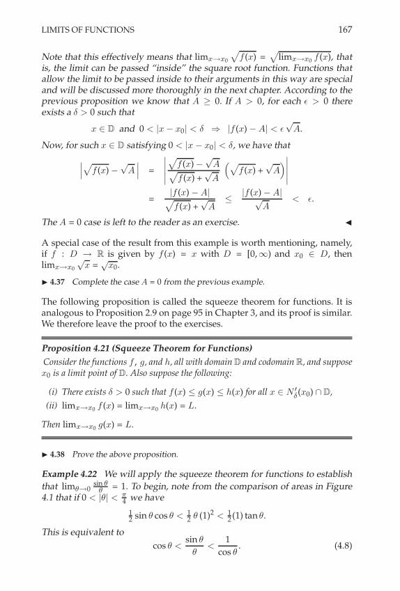
LIMITS OF FUNCTIONS 167
Note that this effectively means that limx(x0
%f (x) =
%limx(x0 f (x), that
is, the limit can be passed “inside” the square root function. Functions thatallow the limit to be passed inside to their arguments in this way are specialand will be discussed more thoroughly in the next chapter. According to theprevious proposition we know that A ! 0. If A > 0, for each ! > 0 thereexists a . > 0 such that
x # D and 0 < |x " x0| < . ) |f (x) " A| < !,
A.
Now, for such x # D satisfying 0 < |x " x0| < ., we have that
&&&%
f (x) ",
A&&& =
&&&&&
%f (x) "
,
A%f (x) +
,
A
(%f (x) +
,
A)&&&&&
=|f (x) " A|%f (x) +
,
A+
|f (x) " A|
,
A< !.
The A = 0 case is left to the reader as an exercise. "
A special case of the result from this example is worth mentioning, namely,if f : D 3 R is given by f (x) = x with D = [0,-) and x0 # D, thenlimx(x0
,
x =,
x0.
! 4.37 Complete the case A = 0 from the previous example.
The following proposition is called the squeeze theorem for functions. It isanalogous to Proposition 2.9 on page 95 in Chapter 3, and its proof is similar.We therefore leave the proof to the exercises.
Proposition 4.21 (Squeeze Theorem for Functions)
Consider the functions f , g, and h, all with domain D and codomain R, and supposex0 is a limit point of D. Also suppose the following:
(i) There exists . > 0 such that f (x) + g(x) + h(x) for all x # N &+(x0) & D,
(ii) limx(x0 f (x) = limx(x0 h(x) = L.
Then limx(x0 g(x) = L.
! 4.38 Prove the above proposition.
Example 4.22 We will apply the squeeze theorem for functions to establishthat lim"(0
sin "" = 1. To begin, note from the comparison of areas in Figure
4.1 that if 0 < |$| < $4 we have
12 sin $ cos $ < 1
2 $ (1)2 < 12 (1) tan $.
This is equivalent to
cos $ <sin $
$<
1
cos $. (4.8)

168 FUNCTIONS: DEFINITIONS AND LIMITS
1
sin!!
tan!
Figure 4.1 Demonstration that lim%&0sin %
%= 1.
We saw in a previous exercise that lim"(0 cos $ = 1, and so application ofthe squeeze theorem for functions to the double inequality (4.8) yields theresult. "
Our final order property results pertaining to limits of real-valued functionshave to do with one-sided limits. In particular, for f : (a, b) 3 R and x0 #
[a, b), we wish to investigate the behavior of f (x) as x 3 x0 from the right,i.e., through values of x > x0. Similarly, for x0 # (a, b], we wish to investigatethe behavior of f (x) as x 3 x0 from the left, i.e., through values of x < x0. Acareful look at Definition 4.1 on page 156 will show that such one-sided limitsare already well defined, since that definition handles the case where x0 is alimit point. Of course, this includes limits such as limx(a f (x) or limx(b f (x)for a function f : (a, b) 3 R. However, we make this idea more explicit in thecase of real-valued functions through the following special definition.
Definition 4.23 Consider f : D13 R, and x0 such that for any r > 0,
D1& (x0, x0 + r) $= !. We write
limx(x+
0
f (x) = A
if for any ! > 0 there exists a . > 0 such that
x # D1& (x0, x0 + .) ) |f (x) " A| < !.
When it exists, the limit A is called the right-hand limit of f as x approachesx0, or the limit of f as x approaches x0 from the right. Similarly, for x0 such thatfor any r > 0, D1
& (x0 " r, x0) $= !, we write
limx(x"
0
f (x) = B
if for any ! > 0 there exists a . > 0 such that
x # D1& (x0 " ., x0) ) |f (x) " B| < !.
When it exists, the limit B is called the left-hand limit of f as x approachesx0, or the limit of f as x approaches x0 from the left.

LIMITS OF FUNCTIONS 169
Note from the above definition that the right-hand limit of f might exist atx0 even though the function f might not be defined at x0. Similarly for theleft-hand limit of f at x0. Also, while we will not formalize these ideas ina separate definition, note in the definition of right-hand limit that the con-dition on x0 that for any r > 0, D1
& (x0, x0 + .) $= ! ensures that x0 is a“right-hand limit point” of D1. Similarly, in the case of the left-hand limit thecorresponding condition on x0 that for any r > 0, D1
& (x0 " ., x0) $= ! en-sures that x0 is a “left-hand limit point” of D1. A limit point x0 of D1 is eithera right-hand limit point of D1, a left-hand limit point of D1, or both a right-and left-hand limit point of D1.
As one might expect, a natural relationship exists between the limit of f andthe right- and left-hand limits of f as x 3 x0.
Proposition 4.24 Consider f : D13 R.
a) If limx#x+
0
f (x) and limx#x"0
f (x) both exist and equal L # R, then
limx(x0 f (x) exists and equals L.
b) Suppose x0 is such that for any r > 0, D1& (x0 " r, x0) $= !, and
D1& (x0, x0 + r) $= !. If limx(x0 f (x) = L exists, then limx(x+
0f (x)
and limx(x"
0f (x) exist and equal L.
! 4.39 Prove the previous proposition.
! 4.40 Suppose f : D1 , R and x0 are such that limx&x0 f (x) = L exists. Must
f have both left- and right-handed limits? (Yes, if the set has appropriate nonemptyintersections.)
Example 4.25 Suppose f : (0, 5) 3 R is given by
f (x) =
E2 x " 1 for 0 < x + 3
5 " x for 3 < x < 5.
We will investigate the left- and right-hand limits of f as x approaches 3.Considering the left-hand limit first, note that for 0 < x + 3,
|f (x) " 5| = |2 x " 1 " 5| = |2 x " 6| = 2 |x " 3|.
This last expression will be less than any given ! > 0 if |x " 3| < . = (2 . That
is, for ! > 0 take . = (2 to obtain
x < 3 and 0 < |x " 3| < . ) |f (x) " 5| < !.
Hence, the left-hand limit is 5. Considering the right-hand limit now, notethat for 3 < x < 5,
|f (x) " 2| = |5 " x " 2| = |3 " x| = |x " 3|.
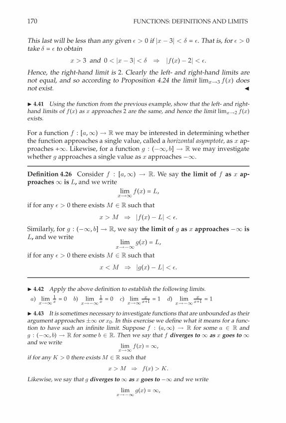
170 FUNCTIONS: DEFINITIONS AND LIMITS
This last will be less than any given ! > 0 if |x " 3| < . = !. That is, for ! > 0take . = ! to obtain
x > 3 and 0 < |x " 3| < . ) |f (x) " 2| < !.
Hence, the right-hand limit is 2. Clearly the left- and right-hand limits arenot equal, and so according to Proposition 4.24 the limit limx(3 f (x) doesnot exist. "
! 4.41 Using the function from the previous example, show that the left- and right-hand limits of f (x) as x approaches 2 are the same, and hence the limit limx&2 f (x)exists.
For a function f : [a,-) 3 R we may be interested in determining whetherthe function approaches a single value, called a horizontal asymptote, as x ap-proaches +-. Likewise, for a function g : ("-, b] 3 R we may investigatewhether g approaches a single value as x approaches "-.
Definition 4.26 Consider f : [a,-) 3 R. We say the limit of f as x ap-proaches - is L, and we write
limx('
f (x) = L,
if for any ! > 0 there exists M # R such that
x > M ) |f (x) " L| < !.
Similarly, for g : ("-, b] 3 R, we say the limit of g as x approaches "- isL, and we write
limx("'
g(x) = L,
if for any ! > 0 there exists M # R such that
x < M ) |g(x) " L| < !.
! 4.42 Apply the above definition to establish the following limits.
a) limx&%
1x
= 0 b) limx&!%
1x
= 0 c) limx&%
x
x+1 = 1 d) limx&!%
x
x+1 = 1
! 4.43 It is sometimes necessary to investigate functions that are unbounded as theirargument approaches ±/ or x0. In this exercise we define what it means for a func-tion to have such an infinite limit. Suppose f : (a, /) , R for some a " R andg : (&/, b) , R for some b " R. Then we say that f diverges to / as x goes to /and we write
limx&%
f (x) = /,
if for any K > 0 there exists M " R such that
x > M - f (x) > K.
Likewise, we say that g diverges to / as x goes to &/ and we write
limx&!%
g(x) = /,

SUPPLEMENTARY EXERCISES 171
if for any K > 0 there exists M " R such that
x < M - g(x) > K.
Similar definitions exist for functions that approach &/ in the limit as x approacheseither / or &/. Write them. It is also possible for functions to grow without boundtoward / or &/ as x approaches a finite limit x0. We say in such cases that the func-tion has a vertical asymptote at x0. Write these definitions as well. Finally, while it isalso possible for a function f : R
k , R to have an infinite limit such as limx&x0f (x) =
/, or limx&x0f (x) = &/, we will not try to formalize the notion of a vector-valued
function having an infinite limit. Why is that?
! 4.44 Evaluate or verify the following limits.
a) limx&%
ex = / b) lim
x&!%ex = 0 c) lim
x&%e
x!e"x
ex+e"x d) limx&!%
ex!e
"x
ex+e"x
e) limx&0
ex!1x
= 1
5 SUPPLEMENTARY EXERCISES
1. Specify the domain, codomain, and range for the function f : R3 , R
2, given bythe rule f (x, y, z) = (x + y + z, xyz).
2. Consider f (z) = z. Find u(x, y) and v(x, y), and determine the domain, codomain,and range of f .
3. Consider the complex function given by the rule f (z) = |z|. Find u(x, y) and v(x, y),and determine the domain, codomain, and range of f .
4. Consider the function f : R \ {0} , R given by f (x) = x + 1x
. What is f (A) for thefollowing sets? a) A = (0, 1) b) A = [1, 2] c) A = (1, /)
5. If f : R \ {0} , R is given by f (x) = 1x
, what is f!1(B) if B = [0, 2)?
6. In Example 2.2 on page 140, let B = {x " R2 : |x| = 1}. Find f
!1(B).
7. Consider the same function as in Example 2.4 on page 141, namely, f : C\{&1} ,C given by f (z) = z!1
z+1 . Find the image of the points on the circle of radius a centeredat the origin for the two cases 0 < a < 1 and 1 < a.
8. Suppose f : X , X is given by f (x) = ax + b where a " R such that a %= 0, andb " X. Show that f is one-to-one and onto.
9. Suppose f : X , R is given by f (x) = a · x + b where a " X such that a %= 0, andb " R. Is f one-to-one? Is it onto? (Yes in both cases.)
10. For the function f : C , C given by f (z) = ez ,
a) What happens to horizontal lines under this mapping?
b) What happens to vertical lines under this mapping?

172 FUNCTIONS: DEFINITIONS AND LIMITS
c) What happens to the strip S = {z " C : 1 # Re(z) # 4}?
11. Consider the function f : C \ {&1} , C given by f (z) = z!1z+1 once more. Find
f (A) where A is the set given by the following (in part c), a " R is fixed):
a) A = {z " C : |z| = 2} b) A = {z " C : |z| = 12} c) A = {z " C : |z| ' a}
12. Let f : R , R2 be given by f (x) = (x, x2). Find f (A) for the following:
a) A = [0, 1] b) A = (&/, /)
13. Suppose f : C , R is given by f (z) = |z|. Find f (A) for the following:
a) A = {z " C : |z| = 5} b) A = {z " C : Re(z) = 2} c) A = {z " C : Im(z) = 2}
14. For the complex function f : D , C, suppose you know that f (z) = f (z) for allz " D. What does this tell you about the function f? (Hint: Think of f as f = u + i v.)
15. Consider f : C \ {0} , C given by f (z) = z + 1z
. If A is the unit circle in thecomplex plane centered at the origin, find f (A). (Hint: Consider the points on thecircle in polar form.)
16. Consider f : R , R given by f (x) = x2. Is f
!1(Q) = Q? (No.) Is f!1(Q) = R?
(No.) Is f!1(I) = I? (Yes.) Is f
!1(I) = R? (No.)
17. Consider f : R2 , R given by f (x, y) = x
2 + y, and suppose B = (0, 1). Findf!1(B).
18. Consider a function f : D , Y. Find the following:
a) f (!) b) f!1(!) c) f
!1(Y)
19. Find an example where equality in part 6 of Proposition 2.5 on page 141 does nothold.
20. For each of the following pairs of sets, determine whether one is a subset of theother, or if they are equal.
a) f (A + B) , f (A) + f (B) b) f!1(B), f!1(B) c)
0f!1(B)
1#, f
!1 ,B
#-
d) f (A), f (A)
21. Show that f : C , R given by f (z) = e!|z|2 is bounded on C.
22. Suppose g : R2 , C and f : C , R are given by g(x, y) = x
2 & i y and f (z) = |z|,respectively. Find f 3 g and identify its domain and codomain.
23. Determine whether each of the following functions is one-to-one.
a) f : R \ {& c
b} , R given by f (x) = a
bx+cwhere a, b, c " R and b %= 0.
b) f : C \ {1} , C given by f (z) = z
z!1 .

SUPPLEMENTARY EXERCISES 173
24. Consider the function f : R , R given by f (x) = 2x. Show that f is increasing,and therefore one-to-one. Determine the range of f . Is f onto? (No.)
25. Let f : R2 , R
3 be given by f (x1, x2) = (x1, x1 + x2, 2x2 ) . Is f one-to-one?
26. Give an example of a function that is one-to-one but not strictly monotone.
27. Determine whether the function f : R3 , R
2 given by f (x, y, z) = (x + y + z, xyz)is one-to-one and/or onto.
28. Consider f : R2 , R
2 given by f (x) = (x1 + x2, x1 & x2) where x = (x1, x2) . Is f
onto? (Yes.)
29. Consider f : R2 , Y ! R
2 given by f (x) = (x1 + x2, x1x2) where x = (x1, x2) .Find a space Y ! R
2 that makes f onto.
30. We define the complex tangent function by tan z . sin z
cos z. The other complex
trigonometric functions are defined in terms of the sine and cosine in a similar man-ner. Find the domain and range of the following: tan z, cot z, sec z, and csc z. Also,show that 1 + tan2
z = sec2z and that 1 + cot2
z = csc2z.
31. Define sin!1z in the natural way by letting w = sin!1
z if and only if z = sin w =e
i w!e"i w
2 iand solving for w. Show that sin
(sin!1
z
)= z. However, sin!1 (sin z) is
not just equal to z. Why?
32. Define cos!1z, tan!1
z, cot!1z, sec!1
z, and csc!1z in the natural way.
33. Define the complex hyperbolic sine and cosine functions sinh : C , C andcosh : C , C according to
sinh z . ez & e
!z
2, and cosh z . e
z + e!z
2.
Show that cosh2z & sinh2
z = 1 for all z " C.
34. Define sinh!1z and cosh!1
z in the natural way.
35. Show that the function f : C\{1} , C\{1} given by f (z) = z+1z!1 in Example 2.22
on page 147 is, in fact, a one-to-one correspondence.
36. In Example 2.22 on page 147, we saw that the function in the previous exercise isits own inverse. Can you think of another function that is its own inverse?
37. Is the function f : C , C given by f (z) = e!z
2
bounded on C? (No.)
38. Let f : R2 \ {0} , R
2 be given by f (x) =(
x21
|x| ,x
22
|x|
)for any x = (x1, x2) " R
2,
and let xn =, 1
n2+1 , 1n
-for n ' 1. Show that limn&% f (xn) = 0.
39. Suppose f : R \ {&1} , R is given by f (x) = x3+1
x+1 . Prove that limx&!1x
3+1x+1 = 3.

174 FUNCTIONS: DEFINITIONS AND LIMITS
40. Suppose f : R , R2 is given by f (x) =
,x
2, x+1x!1
-. Prove that limx&2 f (x) = (4, 3).
41. Suppose f : R \ {0, &1} , R3 is given by f (x) =
,1, 1
x, x
2+1x+1
-. Prove that
limx&!1 f (x) = (1, &1, &2).
42. Rework the last two exercises using Proposition 4.13 on page 161.
43. A function f : R , R is called even if f (&x) = f (x) for all x. What is the relationbetween the left-hand and right-hand limits of an even function at 0? A function f :R , R is called odd if f (&x) = &f (x) for all x. Answer the same question for oddfunctions.
44. Prove that any function f : R , R is the sum of an even and an odd function.(See the previous exercise for the definitions.)
45. Suppose P : C , C is a polynomial and P (sin z) . 0. Prove that P is the zeropolynomial. Prove a similar result for cos z and e
z .
46. Let {an} for n ' 0 be a sequence in X. Define f : [0, /) , X by the formula:f (x) . an, if n # x < n + 1. What is limx&% f (x) if it exists? When does it exist?
47. Define f : R , R such that f (x) = 1 if x " Q, and f (x) = 0 otherwise. Describethe limits of f .
48. Recall that f : C \ {&1, 1} , C given by f (z) = z2+1
z2!1 has the limit limz&0 f (z) =
&1. Find a deleted neighborhood N#r(0) such that f is bounded on N
#r(0) $ D where
D . C \ {&1, 1}.
49. In Example 4.8 on page 159 we showed that limx&0 f (x) = 0. Find a deletedneighborhood of 0 where f is bounded.
50. Suppose f : R\{0} , R2 is given by f (x) =
,x
3!2 x
x, x
2-. Prove that limx&0 f (x) =(&2, 0).
51. Suppose f : R \ {&1, 0} , R3 is given by f (x) =
,x
2!1x+1 , x
2+x
x+1 , 1x
-. Prove that
limx&!1 f (x) = (&2, &1, &1).
52. Consider f : C\{&1} , C given by f (z) = z2!1z+1 . Use Proposition 4.15 on page 163
to find the limit limz&!1 f (z).
53. Use Proposition 4.15 to show that, for n " N, limx&1x
n!1x!1 = n.
54. What are the domains and codomains of the functions in a) through e) of Propo-sition 4.17 on page 163?
55. Consider the function given by f (z) = z2+1
z2!1 on D = C \ {&1, 1} from Example 4.3on page 157. Determine the limit limz&0 f (z) by applying Proposition 4.18 on page165, and compare it to the example.

SUPPLEMENTARY EXERCISES 175
56. Determine the following limits if they exist.
a) limx&01!cos x
xb) limz&0
1!cos z
zc) limz&0
sin z
z
57. Suppose f : R \ {1} , R is given by f (x) =
E3 x &/ < x < 1
2 x & 4 1 # x < /. Show
that limx&1" f (x) = 3 and limx&1+ f (x) = &2.
58. Consider f : R \ {0} , R be given by f (x) = x sin(
1x
). Find
a) limx&0" f (x) b) limx&0+ f (x)
59. Let f : R , R be given by f (x) =
RST
SU
12 if x " (&/, 0),
0 if x " [0, /) $ Q,
1 if x " (0, /) $ I.Find: a) limx&0" f (x) b) limx&0+ f (x)
60. Evaluate or verify the following limits.
a) limx&%
sin x
xb) lim
x&!%sin x
xc) lim
x&%x sin x
d) limx&%
x cos x
x+1 e) limx&%
(x
2 + x + 1)
= / f ) limx&!%
(x & x
2)
= &/.
61. Using the real exponential function and its inverse, the natural logarithm function,define y
x for any pair of real numbers, x " R and y > 0. Extend this definitionappropriately for the case y < 0.
62. Definition of zw .
Recall that for x, y " R with x > 0, we have that xy = e
ln(xy) = ey ln x. With our new
definitions of ez and log z, we may extend this idea as follows. Suppose w " C is
fixed and that z " C is nonzero. Then we define
zw . e
w log z . (4.9)
Note that since log z is multiple valued, zw is also multiple valued. To illustrate this
fact, we determine the values of ii. Using (4.9), we have
ii = e
i log i = ei [ln 1+i ( !
2 +2#k)] = e!( !
2 +2#k), where k " Z.
For parts a) through g) below, determine the values of zw :
a) i!i
b) i1/4
c) (&i)1/3d) 31+i
e) (*
2)2!if ) (
*2 & i)
23 +2i
g) 5"
2!i
h) Recall that we already have a single-valued definition for zn where n " Z (z %= 0 if
n < 0). Does the new definition given by (4.9) above agree with the old one whenn " Z even though the new definition is multiple valued?
i) How many values does zp/q have where z %= 0 and p/q is a rational number in
lowest terms?
j) How many values does z# have where z %= 0?
k) Relate your findings above with our discussion of the nth roots of unity given inChapter 1.

176 FUNCTIONS: DEFINITIONS AND LIMITS
l) Consider our definition of ez given earlier in this chapter. Verify that it is consistent
with the definition of zw given here (that is, though we didn’t define it this way,
ez can be interpreted as a complex number raised to another complex number, just
as zw is). Also verify that e
z is single-valued via (4.9).
m) Just as in the case of the complex logarithm, we may define the principal value ofz
w asz
w . ew Logz . (4.10)
According to (4.10), the principal value of ii is e
!#/2. Assuming z %= 0, does theprincipal value of z
w obey the traditional rules of exponents given by zw1z
w2 =
zw1+w2 and z
w1
zw2 = zw1!w2 ?
n) Define the function F : C , C by
F (z) =
Ee
12 Logz if z %= 0,
0 if z = 0.
Does F agree with our definition of the complex square root function on page 149?
o) Define the complex nth root function in the obvious way.

5FUNCTIONS: CONTINUITY AND
CONVERGENCE
The continuous function is the only workable and usable function. It alone is subjectto law and the laws of calculation. It is a loyal subject of the mathematical kingdom.Other so-called or miscalled functions are freaks, anarchists, disturbers of the peace,malformed curiosities which one and all are of no use to anyone, least of all to theloyal and burden-bearing subjects who by keeping the laws maintain the kingdomand make its advance possible.
E.D. Roe, Jr.
In this chapter, we formally define what it means for a function to be continu-ous at a point or on a set. As we will see, continuous functions have many niceproperties. We will also consider a special type of continuity called uniformcontinuity. Functions that are uniformly continuous are even nicer in certainways than functions that are only continuous. We will also apply the limitconcept to a sequence of functions, and in this way effectively generalize thenotion of sequence, and that of convergence, to “points” that are functions ina function space. Within this context, we take special note of a type of conver-gence called uniform convergence, and determine the particular consequencesto which this type of convergence can lead. Finally, we will consider seriesof functions. While the idea of a series of functions is analogous to that of aseries of numbers or a series of vectors, there are some subtleties to explore.Later, series of functions will play a more prominent role in our developmentof analysis.
1 CONTINUITY
1.1 Definitions
We begin by defining what it means for a function to be continuous at a point.
177

178 FUNCTIONS: CONTINUITY AND CONVERGENCE
Definition 1.1 Consider the function f : D 3 Y.
1. We say that f is continuous at the point x0 # D if for any ! > 0,there exists a . > 0 such that
x # D and |x " x0| < . ) |f (x) " f (x0)| < !.
2. If f is continuous at every point x0 # S ' D, we say that f iscontinuous on S.
We follow Definition 1.1 with a several important remarks.
1. The . that makes the definition “work” depends, in general, on both ! andon x0. A different choice of either ! or x0 # D might require a different ..This is especially significant as it relates to part 2 of Definition 1.1, whichinvolves the continuity of f on a set of points, not just at one particularpoint. We will explore this subtlety in our discussion of the concept ofuniform continuity later in this section.
2. If x0 # D is also a limit point of D, then our definition of continuity atx0 reduces to limx(x0 f (x) = f (x0). In this case, the intuitive idea behindDefinition 1.1 is fairly clear. It states that f is continuous at x0 if whenvalues of x # D get arbitrarily close to x0 the associated values of f (x) getarbitrarily close to f (x0). In this case, one can interpret Definition 1.1 aslimx(x0 f (x) = f (limx(x0 x), i.e., the limit process can be taken “inside”the function f to its argument.
3. If x0 # D is an isolated point of D, then our definition of continuity at x0
holds vacuously. In this case, even the relevance of Definition 1.1 may notseem clear. In fact, however, when x0 # D is an isolated point of D thereexists a deleted neighborhood N &
+(x0) such that N &+(x0) & D = !, and so
there are no points x # D available to contradict the definition of continu-ity. For this reason, if x0 is an isolated point of its domain, f is continuousthere. This seemingly strange conclusion may take some getting used to.
4. If f : D 3 Y is continuous throughout a set S ' D, as described in part 2of the definition, it is not true in general that f maps convergent sequencesin S to convergent sequences in Y. That is, f being continuous on S is notenough to imply that f preserves convergence on S. We refer the readerto the exercises that follow for evidence of this. We will discover that thisconvergence-preserving property is only possessed by functions that areuniformly continuous.
! 5.1 Prove remark 2 above.
! 5.2 As a special case of remark 2, consider the following situation. Suppose f :D , Y is continuous at x0 " D where x0 is a limit point of D. If {xn} ! D is a sequencethat converges to x0, then show that limn&% f (xn) = f (limn&% xn) = f (x0).
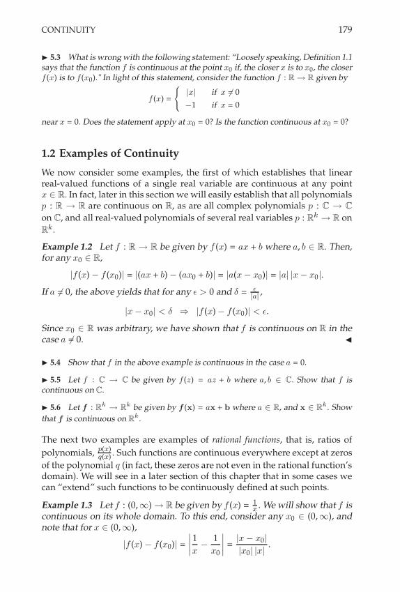
CONTINUITY 179
! 5.3 What is wrong with the following statement: “Loosely speaking, Definition 1.1says that the function f is continuous at the point x0 if, the closer x is to x0, the closerf (x) is to f (x0)." In light of this statement, consider the function f : R , R given by
f (x) =
E|x| if x %= 0
&1 if x = 0
near x = 0. Does the statement apply at x0 = 0? Is the function continuous at x0 = 0?
1.2 Examples of Continuity
We now consider some examples, the first of which establishes that linearreal-valued functions of a single real variable are continuous at any pointx # R. In fact, later in this section we will easily establish that all polynomialsp : R 3 R are continuous on R, as are all complex polynomials p : C 3 C
on C, and all real-valued polynomials of several real variables p : Rk3 R on
Rk.
Example 1.2 Let f : R 3 R be given by f (x) = ax + b where a, b # R. Then,for any x0 # R,
|f (x) " f (x0)| = |(ax + b) " (ax0 + b)| = |a(x " x0)| = |a| |x " x0|.
If a $= 0, the above yields that for any ! > 0 and . = (|a| ,
|x " x0| < . ) |f (x) " f (x0)| < !.
Since x0 # R was arbitrary, we have shown that f is continuous on R in thecase a $= 0. "
! 5.4 Show that f in the above example is continuous in the case a = 0.
! 5.5 Let f : C , C be given by f (z) = az + b where a, b " C. Show that f iscontinuous on C.
! 5.6 Let f : Rk , R
k be given by f (x) = ax + b where a " R, and x " Rk . Show
that f is continuous on Rk .
The next two examples are examples of rational functions, that is, ratios of
polynomials, p(x)q(x) . Such functions are continuous everywhere except at zeros
of the polynomial q (in fact, these zeros are not even in the rational function’sdomain). We will see in a later section of this chapter that in some cases wecan “extend” such functions to be continuously defined at such points.
Example 1.3 Let f : (0,-) 3 R be given by f (x) = 1x . We will show that f is
continuous on its whole domain. To this end, consider any x0 # (0,-), andnote that for x # (0,-),
|f (x) " f (x0)| =
&&&&1
x"
1
x0
&&&& =|x " x0|
|x0| |x|.

180 FUNCTIONS: CONTINUITY AND CONVERGENCE
If we assume that |x " x0| < 12 x0, then |x| ! 1
2 x0, and therefore
|f (x) " f (x0)| + 2x2
0|x " x0| < !,
as long as |x " x0| <( x2
02 . That is, for . = min
212x0,
( x20
2
3, we have that for
x # (0,-),|x " x0| < . ) |f (x) " f (x0)| < !. "
! 5.7 Show in the above example that it is impossible to choose . to be independentof x0. (Hint: For given $ > 0, consider x0 = 1
n $and x = 1
(n+1) $for sufficiently large
n " N.)
! 5.8 Consider f : (0, /) , R given by f (x) = 1x
. Use this example to show that,as claimed in remark 4 after Definition 1.1, not all continuous functions preserve con-vergence.
In the following example, we apply Definition 1.1 to a function of more thanone variable.
Example 1.4 Let D2 = {x = (x, y) # R2 : x > 0, y > 0} and suppose f :D2
3 R is given byf (x) =
x
x + y.
We will show that f is continuous at the point (2, 1), an interior point (andtherefore a limit point) of its domain. To this end, let x = (x, y) # D2. Then
|f (x) " f (2, 1)| =
&&&&x
x + y"
2
3
&&&&
=|(x " 2) + 2 (1 " y)|
3 (x + y)
+
|x " 2|
3 (x + y)+
2 |y " 1|
3 (x + y)
+
|x" (2, 1)|
3 (x + y)+
2 |x" (2, 1)|
3 (x + y)
=|x" (2, 1)|
(x + y).
If we suppose for the moment that |x " (2, 1)| < 12 , then |x " 2| < 1
2 and
|y " 1| < 12 , and so x + y > 2 (Why?), and 1
x+y < 12 . This yields
|f (x) " f (2, 1)| < 12 |x" (2, 1)|,
and the right side of the above inequality will be less than any given ! > 0 as
long as |x" (2, 1)| < min(
2 !, 12
)/ .. That is, overall we have shown that for
any given ! > 0 and x # D2,
|x" (2, 1)| < . ) |f (x) " f (2, 1)| < !.
Therefore, f is continuous at (2, 1). "

CONTINUITY 181
! 5.9 Show that the function f (x) = x
x+yin the last example is continuous at every
point in its domain.
Example 1.5 Consider f : C \ {1} 3 C given by f (z) = z + 1z"1 , and let
zn =(
1+i3
)nfor n # N. We will use the result of Exercise 5.2 to show that
limn(' f (zn) = "1. To do this, we will first show that f is continuous atevery point in its domain. Consider an arbitrary z0 # C \ {1} and note thatfor any other z # C \ {1},
|f (z) " f (z0)| =
&&&&z " z0 +1
z " 1"
1
z0 " 1
&&&&
=
&&&&z " z0 +z0 " z
(z " 1) (z0 " 1)
&&&&
+ |z " z0| +|z " z0|
|z " 1| |z0 " 1|. (5.1)
Now, consider those points z # C that satisfy |z " z0| < 12 |z0 " 1|. For such z,
|z " 1| = |z " z0 + z0 " 1| ! |z0 " 1|" |z " z0| > 12 |z0 " 1|,
and therefore (5.1) becomes
|f (z) " f (z0)| + |z " z0| +|z " z0|
|z " 1| |z0 " 1|
< |z " z0| +2 |z " z0|
|z0 " 1|2
=
21 +
2
|z0 " 1|2
3|z " z0|.
This last expression will be less than ! provided z # D and |z"z0| < ., where
. / min
212 |z0 " 1|, !
(1 + 2
|z0"1|2)"1
3.
This establishes that f is continuous at every z0 # C \ {1}. We now will showthat limn(' zn = 0. To see this, note that
|zn " 0| =&&&(
1+i3
)n&&& =&&& 1+i
3
&&&n
=($
23
)n,
and the above clearly goes to zero as n goes to -. Finally, by remark 2 fol-lowing Definition 1.1, we have
limn('
f (zn) = f,
limn('
zn-
= f (0) = "1."
Example 1.6 Let f : [0,-) 3 R be given by f (x) =,
x. Then for x0 # (0,-)and x # [0,-), we have that
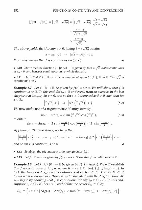
182 FUNCTIONS: CONTINUITY AND CONVERGENCE
|f (x) " f (x0)| =&&,x "
,
x0&& =
&&&&,,
x "
,
x0- ,
x +,
x0,
x +,
x0
&&&&
=|x " x0|,
x +,
x0
<|x " x0|,
x0.
The above yields that for any ! > 0, taking . = !,
x0 obtains
|x " x0| < . ) |
,
x "
,
x0| < !.
From this we see that f is continuous on (0,-). "
! 5.10 Show that the function f : [0, /) , R given by f (x) =*
x is also continuousat x0 = 0, and hence is continuous on its whole domain.
! 5.11 Show that if f : D , R is continuous at x0 and if f ' 0 on D, then*
f iscontinuous at x0.
Example 1.7 Let f : R 3 R be given by f (x) = sin x. We will show that f iscontinuous on R. To this end, fix x0 # R and recall from an exercise in the lastchapter that limx(0 sin x = 0, and so for ! > 0 there exists . > 0 such that forx # R, &&&x"x0
2
&&& < +2 )
&&&sin(
x"x02
)&&& < (2 . (5.2)
We now make use of a trigonometric identity, namely,
sin x " sin x0 = 2 sin,x"x0
2
-cos
,x+x02
-, (5.3)
to obtain| sin x " sin x0| =
&&&2 sin,x"x0
2
-cos
,x+x02
-&&& + 2&&&sin
,x"x02
-&&& .
Applying (5.2) to the above, we have that&&&x"x0
2
&&& < +2 , or |x " x0| < . ) | sin x " sin x0| + 2
&&&sin(
x"x02
)&&& < !,
and so sin x is continuous on R. "
! 5.12 Establish the trigonometric identity given in (5.3).
! 5.13 Let f : R , R be given by f (x) = cos x. Show that f is continuous on R.
Example 1.8 Let f : C\{0} 3 R be given by f (z) = Arg(z). We will establishthat f is continuous on C \ K where K = {z # C : Re(z) + 0, Im(z) = 0}. Infact, the function Arg(z) is discontinuous at each z # K . The set K ' C
forms what is known as a “branch cut” associated with the Arg function. Wewill begin by showing that f is continuous for any z0 # C \ K . To this end,suppose z0 # C \ K . Let ! > 0 and define the sector Sz0 ' C by
Sz0 /
!z # C : |Arg(z) " Arg(z0)| < min
,% " Arg(z0), % + Arg(z0), !
-".

CONTINUITY 183
Note that this ensures that Sz0 ' C\K . Figure 5.1 illustrates the case where z0
lies in the second quadrant of the complex plane. The reader is encouragedto sketch the cases corresponding to z0 lying in the other quadrants to seethe resulting geometry associated with Sz0 . Now choose . > 0 such that
$
z0
Figure 5.1 Demonstration that Arg(z) is continuous.
N+(z0) ' Sz0 . It is easy to see that
z # N+(z0) ) z # Sz0 , i.e., |Arg(z) " Arg(z0)| < !,
which in turn implies that Arg : C \ K 3 C is continuous on its domain. Tosee that f (z) = Arg(z) is not continuous at z0 = "1 (for example), we assumethe opposite and argue by contradiction. If f is continuous at z0 = "1, thenthere exists . > 0 such that
|z + 1| < . ) |Arg(z) " Arg("1)| = |Arg(z) " %| < $4 .
We may choose N # N large enough so that zN / ei("$+ 1N ) is within . of
z0 = "1, that is |zN + 1| < .. (Why?) This yields
|Arg(zN ) " %| = |("% + 1N ) " %| = |2% "
1N | < $
4 ,
a contradiction. The proof that Arg(z) is discontinuous on the rest of K is leftto the reader. "
! 5.14 Complete the proof of the claim in the above example, and show that Arg(z)is discontinuous on all of K.
! 5.15 Why does the proof given in the above example for the continuity of Arg(z)on C \ K not work for z0 " K?
! 5.16 Let f : C , C be given by f (z) =*
z as given in Definition 3.1 on page 149.Show that f is not continuous on all of C. Where is this function continuous?
! 5.17 Let f : C \ {0} , C be given by f (z) = Log(z) as given in Definition 3.6on page 153. Show that f is not continuous on all of C \ {0}. Where is this functioncontinuous?
! 5.18 Consider the function f : R \ {0} , R2 given by f (x) =
(1x
, 2 x2)
. Show
that f is continuous at every point in R \ {0}.

184 FUNCTIONS: CONTINUITY AND CONVERGENCE
! 5.19 Consider the function from the previous exercise, and let xn = 2 n2
n2+1 for n " N.
Show that limn&% f (xn) =(
12 , 8
).
! 5.20 Show that the complex function f : C , C given by f (z) = a z2 + b z + c for
a, b, c " C is continuous on C.
! 5.21 Prove that the real exponential function exp : R , R given by exp(x) = ex is
continuous on its domain.
1.3 Algebraic Properties of Continuous Functions
In this subsection we describe the many convenient properties possessed bycontinuous functions in various settings. We begin with the algebraic prop-erties that allow for simple constructions of more elaborate continuous func-tions from more basic ones.
Proposition 1.9 Consider f and g where both are functions from D to codomainY, and both f and g are continuous at x0 # D. Then
a) f ± y0 is continuous at x0 for any y0 # Y.
b) f ± g is continuous at x0.
c) c f is continuous at x0 for c # R or C.
d) f · g is continuous at x0.
e) f/g is continuous at x0 if f and g are real or complex valued and g is nonzero atx0.
f) |f | is continuous at x0.
Note that in property c), the constant c should be understood as complexonly in the case where f is complex valued. Note also that in property d), themultiplication indicated is the dot product in the case Y = Rp, and the usualmultiplication in R or C otherwise.
! 5.22 Prove the previous proposition.
! 5.23 Does property d) in the above proposition still hold if f has codomain R
while g has codomain Rp?
! 5.24 In property e), is it necessary that f be real or complex valued? Explain.
! 5.25 Prove that the following functions f : R , R are continuous on R.
a) f (x) = c for c " R b) f (x) = x c) f (x) = xn for n " Z
+
d) f (x) = c0 + c1 x + c2 x2 + · · · + cn x
n for cj " R and n " N with cn %= 0.
This establishes that all real polynomials are continuous on R.
! 5.26 Generalize the conclusion of the previous two exercises to the complex func-tion case. That is, show that complex polynomials are continuous on C and complexrational functions are continuous on their domains.

CONTINUITY 185
! 5.27 Prove that the following functions f : R2 , R are continuous on R
2.
a) f (x, y) = c for c " R b) f (x, y) = x c) f (x, y) = y
d) f (x, y) = xn for n " Z
+ e) f (x, y) = yn for n " Z
+
f) f (x, y) = cij xiy
j for i, j " Z+ and cij " R
g) f (x, y) =+
1'i,j'm
cij xiy
j
This establishes that real-valued polynomials in two real variables are continuous onall of R
2.
! 5.28 Generalize the previous exercise to the case of f : Rk , R.
! 5.29 Let f : D2 , R be given by f (x, y) = p(x,y)
q(x,y) where p : R2 , R and q : R
2 , R
are of the form described in part g) of the previous exercise, and D2 = {(x, y) "
R2 : q(x, y) %= 0}. Show that f is continuous on D
2. This establishes that real-valuedrational functions of two real variables are continuous on all of R
2 \ Zq where Zq isthe set of zeros of q(x, y).
! 5.30 Generalize the previous exercise to the case of the rational function f : Dk ,
R given by f (x1, . . . , xk) = p(x1,...,xk)q(x1,...,xk) defined on D
k given by Dk = {(x1, . . . , xk) "
Rk : q(x1, . . . , xk) %= 0}.
! 5.31 Consider f : D , Rp where f (x) = (f1(x), f2(x), . . . , fp(x)) for each x " D,
and fj : D , R for 1 # j # p. Show that f is continuous at x0 " D if and only iffj is continuous at x0 " D for each 1 # j # p. What does this say about the complexfunction case f : D , C with z0 " D?
Example 1.10 Let f : C 3 C be given by f (z) = sin z. We will establish thatf is continuous on C. To this end, note that
f (z) = sin z =,
ey+e"y
2
-sin x + i
,e"y"ey
2
-cos x. (Why?)
Since Re (f (z)) and Im (f (z)) are continuous functions of (x, y) (Why?), it fol-lows that f (z) is continuous in z. "
! 5.32 Answer the two (Why?) questions in the previous example.
! 5.33 Consider f : C , C given by f (z) = cos z. Show that f is continuous on C.
As described in an earlier chapter, each of Y1 and Y2 in the statement of thefollowing proposition should be understood to be any of the spaces R, Rp, orC. The proposition basically states that a continuous function of a continuousfunction is a continuous function.
Proposition 1.11 Let f and g be functions such that f : D 3 Y1 has range givenby Rf = f (D), and g : Rf 3 Y2. Suppose also that f is continuous at x0 # D, andg is continuous at y0 = f (x0) # Rf . Then the composite function g ; f : D 3 Y2 iscontinuous at x0 # D.

186 FUNCTIONS: CONTINUITY AND CONVERGENCE
PROOF Suppose ! > 0 is given. Then there exists , > 0 such that
y # Rf and |y " y0| < , ) |g(y) " g(y0)| < !.
Similarly, for this same , > 0 there exists . > 0 such that
x # D and |x " x0| < . ) |f (x) " f (x0)| < ,.
For y = f (x) we have |g(y) " g(y0)| = |g(f (x)) " g(f (x0))| and |f (x) " f (x0)| =|y " y0|. From this we see that for any given ! > 0 there exists a . > 0 suchthat
x # D and |x " x0| < . ) |g(f (x)) " g(f (x0))| < !,
and the proposition is proved. #
Example 1.12 Consider the function h : Rk3 R given by h(x) = e"|x|2 .
Let f : Rk3 R be given by f (x) = "|x|2, and let g : Rf 3 R be given by
g(x) = ex. By a previous exercise we know that g is continuous on R, andtherefore is continuous on Rf . The reader should verify that f is continuous
on Rk . By Proposition 1.11, it follows that h = g ; f is continuous on Rk . "
! 5.34 Show that the function f : Rk , R given by f (x) = &|x|2 is continuous on
Rk .
The following proposition is an unsurprising consequence of the continuityof f : Dk
3 Y, a function of a vector. It basically states that if f is a con-tinuous function of the vector x, then f is continuous in each component ofx. One should be careful, however, in noting that the converse is not true ingeneral.
Proposition 1.13 Suppose f : Dk3 Y is continuous at a = (a1, . . . , ak) #
Dk . Let Dj /
!xj # R : (a1, . . . , aj"1, xj , aj+1, . . . , ak) # Dk
", and define the
function f (j) : Dj 3 Y by
f (j)(xj ) / f (a1, . . . , aj"1, xj , aj+1, . . . , ak) for 1 + j + k.
Then f (j) is continuous at xj = aj .
PROOF Since f is continuous at a, given any ! > 0 there exists . > 0 suchthat
x # Dk and |x " a| < . ) |f (x) " f (a)| < !.
Note that if xj # Dj then xj / (a1, . . . , aj"1, xj , aj+1, . . . , ak) # Dk , and that
f (j)(xj ) = f (xj). All of this yields
xj # Dj and |xj " aj | < . ) xj # Dk and |xj " a| < ..
Therefore,
xj # Dj and |xj " aj | < . ) |f (xj) " f (a)| = |f (j)(xj ) " f (j)(aj)| < !,
that is, f (j) is continuous at xj = aj . #

CONTINUITY 187
To illustrate that the converse of Proposition 1.13 is not true in general, wegive the following example.
Example 1.14 Consider f : R23 R given by
f (x, y) =
E2 x yx2+y2 if (x, y) $= (0, 0)
0 if (x, y) = (0, 0).
This function is not continuous at (0, 0), since
f (t, t) = 2 t2
t2+t2 = 1 if t $= 0,
and f (0, 0) = 0. However, if x = c is fixed, then
f (2)(y) / f (c, y) = 2 c yc2+y2
is a continuous function of y for each value of c. Similarly, if y = k is fixed,then the corresponding function
f (1)(x) / f (x, k) = 2 k xx2+k2
is a continuous function of x for each value of k. "
The above example illustrates that a function of a vector may be continu-ous in each component of the vector separately, with the other componentsheld fixed, but it may not be continuous as a function of the vector accordingto Definition 1.1. We sometimes refer to such a function as being separatelycontinuous in each variable, but not jointly continuous.
1.4 Topological Properties and Characterizations
We now consider how the continuity of a function f : D 3 Y is related to thetopology of the sets D and Y. In particular, bounded sets, open sets, compactsets, and connected sets have special significance as they relate to continu-ous functions. Before we state our first result, recall from Chapter 2 that forD ' X, a subset U ' D is open in D if U = D & V for some open set V ' X.Also, U is said to be closed in D if D \ U is open in D.
We begin by showing that if a function is continuous at a point x0, then itmust be bounded on a neighborhood of that point.
Proposition 1.15 Suppose f : D 3 Y is continuous at x0 # D. Then there exists. > 0 such that f is bounded on N+(x0) & D.
PROOF Since f is continuous at x0, there exists a . > 0 such that if x # D
and |x " x0| < ., i.e., if x # N+(x0) & D, then |f (x) " f (x0)| < 1. Applicationof the triangle inequality then yields that
x # N+(x0) & D ) |f (x)| < 1 + |f (x0)|,
and the proposition is proved. #

188 FUNCTIONS: CONTINUITY AND CONVERGENCE
! 5.35 Does Proposition 1.15 simply follow from Proposition 4.11 on page 160?
! 5.36 Prove the following corollary to Proposition 1.15: Suppose f : D , Y iscontinuous at x0 " D where x0 is an interior point of D. Then there exists a . > 0 suchthat f is bounded on N&(x0).
Our next result states that a function f is continuous on its domain if andonly if inverse images of open sets in its codomain are open in its domain.Stated more concisely, “f is continuous if and only if inverse images of opensets are open sets."
Theorem 1.16 The function f : D 3 Y is continuous on D if and only if for anyset U open in Y the set f"1 (U ) is open in D.
PROOF We prove the case where Y is all of R, Rp, or C, and leave the casewhere Y is a proper subset of one of these spaces to the reader. Supposef : D 3 Y is continuous on D, and let U be an open subset of Y. We mustshow that f"1(U ) is open in D, i.e., that f"1(U ) = D & V for some open setV in X. To see this, consider an arbitrary x0 # f"1 (U ) . Then f (x0) # U , andsince U is open in Y, there exists a neighborhood Nr (f (x0)) ' U . Since f iscontinuous at x0, there exists a . > 0 such that
x # D and |x " x0| < . ) |f (x) " f (x0)| < r.
That is,x # D & N+(x0) ) f (x) # Nr (f (x0)) ' U .
This implies that x # f"1(U ), and so
D & N+(x0) ' f"1(U ). (5.4)
Note that every x0 # f"1(U ) has a neighborhood N+(x0) such that (5.4) istrue, and note also that . will in general depend on x0. Finally, define V byV /
#x0#f"1(U ) N+(x0). It then follows from (5.4) that D & V ' f"1(U ). Since
it is also true that any x # f"1(U ) must also be in D&V (Why?), we have thatf"1(U ) = D & V , and hence, f"1(U ) is open in D. For the converse, supposethat f : D 3 Y is such that f"1(U ) is open in D for every open subset U ' Y.Fix x0 # D, and consider an arbitrary ! > 0. We must find . > 0 such that
x # D and |x " x0| < . ) |f (x) " f (x0)| < !,
that is,x # D & N+(x0) ) f (x) # N( (f (x0)) .
Note that N( (f (x0)) is open in Y, and therefore f"1 [N( (f (x0))] = D & V ,where V is open in X. Since x0 # f"1 [N( (f (x0))], it follows that x0 # D & V ,and since V is open in X there exists a . > 0 such that N+(x0) ' V . Finally, ifx # D & N+(x0), we have that x # D & V , and, since D & V = f"1 [N( (f (x0))],that f (x) # N( (f (x0)) . #

CONTINUITY 189
! 5.37 Answer the (Why?) question in the above proof, and then prove the case ofthe above theorem where Y is a proper subset of R, R
p, or C.
! 5.38 Note that the condition on U that it be “open in Y" cannot be changed to“open and a subset of Y." Trace through the example of the function f : R , Y
given by f (x) =
E&1 if x < 0
1 if x ' 0, with Y = {&1, 1} to see why. In this example, the
conditions of the altered theorem would be satisfied, but the conclusion obviouslydoesn’t hold for f .
Example 1.17 Suppose f : R 3 R has the property that f"1(I) is open forevery open interval I ' R. We will show that f must be continuous on R.To this end, let B ' R be an open set. From Proposition 3.6 on page 57 weknow that B =
#I& where {I&} is a collection of open intervals in R. Since
f"1(B) = f"1 (#
I&) =#
f"1(I&), and since f"1(I&) is open for each ', itfollows that f"1(B) is also open. Hence, f is continuous. "
! 5.39 Does Example 1.17 generalize to functions f : Rk , R? How about to func-
tions f : Rk , R
p? How about to complex functions f : C , C?
! 5.40 Show that f : D , Y is continuous on D if and only if f!1(B) is closed in D
for every B closed in Y.
Yet another equivalence for the continuity of f on D is given by the followingresult. While its meaning may be unclear initially, it will be useful in provingthe next result whose meaning is clearer.
Proposition 1.18 The function f : D 3 Y is continuous on D if and only iff,A-' f (A) for every subset A ' D.
PROOF We consider the case where D = X and Y is all of R, Rp, or C, leavingthe more general case to the reader. Suppose f : D 3 Y is such that f
,A-'
f (A) for every subset A ' D. We will show that f"1(B) is closed in D forevery B closed in Y. By Exercise 5.40, this will establish the continuity of fon D. To this end, suppose B is a closed subset of Y and let A = f"1(B). Tosee that A is closed in D, let x # A. Then
f (x) # f,A-' f (A) ' B = B,
and therefore x # f"1(B) = A. We have shown that A ' A, which impliesthat A is closed. Now assume f : D 3 Y is continuous on D. Let A ' D
and y0 # f (A). Then y0 = f (x0) for x0 # A, and since there exists a sequence{xn} ' A such that lim xn = x0, it follows that the sequence {f (xn)} ' f (A)converges to f (x0), that is, y0 = f (x0) # f (A). This completes the proof in thespecial case. The general case is left to the reader. #

190 FUNCTIONS: CONTINUITY AND CONVERGENCE
! 5.41 Generalize the argument given in the proof above to account for the caseswhere D ! X and Y ! R, R
p, or C.
! 5.42 Can you find an example of a discontinuous function f : D , Y such thatfor some A ! D, f (A) 1 f (A)?
The following proposition establishes a convenient sufficient condition forcontinuity of a function on its domain. In a certain sense, it can be seen as arefinement of remark 2 immediately following the definition of continuity onpage 178. Note the difference between that remark and the conditions statedin the proposition.
Proposition 1.19 Suppose f : D 3 Y is such that for each x # D, lim f (xn) =f (x) for every sequence {xn} ' D that converges to x # D. Then f is continuouson D.
PROOF Let A be any subset of D. We will show that f,A-' f (A). Recall
that according to Proposition 1.18, this is equivalent to f being continuouson D. To establish the result, let x0 # A. Then there exists {xn} ' A such thatlim xn = x0, and therefore lim f (xn) = f (x0). Since f (xn) # f (A), it followsthat f (x0) # f (A), which is equivalent to f (A) ' f (A). #
The next result effectively states that “continuous functions take compact setsto compact sets," that is, “continuous functions preserve compactness."
Theorem 1.20 Let K ' X be a compact set and f : K 3 Y a continuous functionon K . Then f (K) is compact.
PROOF Suppose f (K) '
#& W&, where {W&} is a collection of open sets
in Y. That is,#
& W& is an open cover for f (K). Then K ' f"1,#
& W&-
=#& f"1(W&), and since f"1(W&) is open in K we may write f"1(W&) = K &
V& where V& is open in X. From this, we may conclude that K '
#& V&. But
since K is compact and K '
#& V&, we can extract a finite subcover for K ,
namely, K ' V&1 % V&2 % · · · % V&r . From this we can conclude that
f (K) ' W&1 % W&2 % · · · % W&r .
Therefore, f (K) is compact. #
! 5.43 As claimed in the above proof, verify that K !#
!V! and that f (K) !#
r
i=1 W!i .
Example 1.21 Let a, b > 0 and define K / {(x, y) # R2 : x2
a2 + y2
b2 + 1}, thatis, K is the interior and boundary of an ellipse centered at the origin in theplane. Consider the continuous function f : R2
3 R given by f (x, y) = 1|xy|+1
.
By the previous theorem, we know that the image f (K) must be a compactsubset of R, even if we can’t visualize it. "

CONTINUITY 191
! 5.44 In the previous example, show that f is continuous on R2.
! 5.45 Let f : (0, 1) , R be given by f (x) = 1x
. Note that f is continuous on (0, 1)and f ((0, 1)) = (1, /) is not compact. Does this contradict Theorem 1.20?
! 5.46 Let f : (0, 1) , R be given by f (x) = 1x
sin 1x
. Show that f is continuous on(0, 1). Is f ((0, 1)) compact?
Finally, our last result in this discussion of topological properties and con-tinuous functions states that “continuous functions take connected sets toconnected sets," or “continuous functions preserve connectedness."
Theorem 1.22 Suppose f : D 3 Y is continuous on D. If D is connected, thenf (D) ' Y is connected.
PROOF Suppose f (D) is disconnected. Then f (D) = V % W where V and Ware nonempty and V & W = V & W = !. From this, it follows that
D = f"1(V ) % f"1(W ).
We leave it as an exercise to show that
a) f"1(V ) $= ! and f"1(W ) $= !
b) f"1(V ) & f"1(W ) = f"1(V ) & f"1(W ) = !.
This contradiction (that D is disconnected) shows that f (D) must be con-nected. #
! 5.47 Finish the proof of the above theorem.
Example 1.23 Let g : (0, 1) 3 R be given by g(x) = 1x sin 1
x . Since g iscontinuous and (0, 1) is connected, it follows that g ((0, 1)) = {y # R : y =1x sin 1
x for x # (0, 1)} is also connected. "
1.5 Real Continuous Functions
Here we present some results that are relevant only to real-valued functions.Each depends on the special order properties that, among our Euclideanspaces of interest, are only possessed by the real number system R.
Proposition 1.24 Suppose f : D 3 R is continuous at x0 # D, and supposef (x0) > 0. Then there exists a neighborhood N+(x0) centered at x0 such that f (x) >0 for x # N+(x0) & D.
PROOF By the continuity of f at x0, there exists a . > 0 such that
x # D and |x " x0| < . ) |f (x) " f (x0)| < 12 f (x0).

192 FUNCTIONS: CONTINUITY AND CONVERGENCE
Sincef (x0) " f (x) + |f (x) " f (x0)| < 1
2 f (x0),
we have thatx # D & N+(x0) ) f (x) > 1
2 f (x0) > 0,
and the proposition is proved. #
Note that in the special case where x0 is an interior point of D, the aboveresult can be stated more simply. Namely, if f is continuous at the interiorpoint x0 # D and if f (x0) > 0, then f must be positive throughout someneighborhood of x0.
! 5.48 If f : D , R is continuous at x0 " D and if f (x0) < 0, show that there existsa neighborhood N&(x0) centered at x0 such that f (x) < 0 for all x " D $ N&(x0).
The next result has great practical significance, as every student of calculusknows.
Theorem 1.25 (The Max-Min Theorem)Let K ' X be a compact set, and f : K 3 R a continuous, real-valued function onK . Then f attains a maximum value and a minimum value on K , i.e., there exist x1
and x2 in K such that f (x1) + f (x) + f (x2) for all x # K .
PROOF The set f (K) is compact, and therefore closed and bounded. Let M =sup f (K) and m = inf f (K). Since f (K) is closed, both M and m are in f (K).That is, there exist x1 and x2 in K such that f (x1) = m and f (x2) = M . #
Example 1.26 Consider again D2 = {x = (x, y) # R2 : x > 0, y > 0}, andf : D2
3 R given by f (x) = xx+y . As already seen in a previous example
and a previous exercise, f is continuous at every point in D2. If we takeK = [1, 2] . [1, 4] then K ' D2 and f must attain a maximum and a min-imum somewhere on K . Note that Theorem 1.25 does not provide a meansfor finding these extreme values. "
! 5.49 Even though Theorem 1.25 is not useful in this regard, can you find the max-imum and minimum of the function f from the previous example?
! 5.50 Let K ! X be a compact set, and f : K , Y a continuous function on K.Prove that |f | : K , R attains a maximum value and a minimum value on K.
In some ways the following significant theorem sheds more light on Propo-sition 1.24 on page 191, although it is not as generally applicable as Proposi-tion 1.24.
Theorem 1.27 (The Intermediate Value Theorem)Suppose f : [a, b] 3 R is continuous on [ a, b ] ' R and that f (a) $= f (b). Then forevery y between f (a) and f (b), there exists c # (a, b) such that f (c) = y.

CONTINUITY 193
PROOF We prove a special case and leave the general proof to the reader.Suppose f (a) < 0 and f (b) > 0. We will show that there exists c # (a, b) suchthat f (c) = 0. To this end, let S = {x # [ a, b ] : f (x) < 0}. Then a # S, andsince f is continuous at a there exists a .1 > 0 such that [ a, a + .1) ' S.(Why?) Similarly, b # SC , and there exists a .2 > 0 such that (b" .2, b ] ' SC .
Now let c = sup S. It follows that a + +12 + c + b "
+22 . (Why?) This shows
that c # (a, b). We will now show that f (c) = 0 with a proof by contradiction.Suppose f (c) < 0. Then there exists a .3 > 0 such that (c" .3, c + .3) ' [ a, b ],
where f (x) < 0 for all x # (c " .3, c + .3). But then f(c + +3
2
)< 0, which
implies that c + +32 # S, a contradiction. Therefore f (c) ! 0. But if f (c) > 0,
then there exists a .4 > 0 such that (c " .4, c + .4) ' [ a, b ], where f (x) > 0for all x # (c" .4, c + .4). By the definition of c there must exist ) # (c" .4, c ]such that ) # S, i.e., f ()) < 0. This contradicts the fact that f (x) > 0 on(c " .4, c + .4), and so we must have f (c) = 0. #
! 5.51 Prove the general case of the intermediate value theorem. Why is it not asgenerally applicable as Proposition 1.24?
! 5.52 Is the value c referenced in the intermediate Value theorem unique?
The following examples illustrate an interesting consequences of the inter-mediate value theorem.
Example 1.28 Suppose f : [0, 1] 3 [0, 1] is continuous. We will show thatthere exists at least one point x0 # [0, 1] such that f (x0) = x0. Such a pointis called a fixed point for f . To show this, first note that if f (0) = 0 or iff (1) = 1 then we are done. So assume that f (0) > 0 and that f (1) < 1. Letg(x) = f (x) " x, and note that g is continuous on [0, 1]. Since g(0) > 0 andg(1) < 0, according to the intermediate value theorem there must be a pointx0 # (0, 1) such that g(x0) = 0, i.e., f (x0) = x0. "
Example 1.29 Suppose f : R 3 R is the continuous function given by f (x) =x3
" x + 1. Are there any real roots to the equation f (x) = 0? If so, can theybe identified? While the intermediate value theorem can yield an answer tothe first question, we often can’t get a precise answer to the second. Note thatf ("2) = "5, while f ("1) = 1. Therefore, there exists c # ("2, "1) such thatf (c) = 0. "
! 5.53 Can you think of a procedure for specifying the numerical value of c in theprevious example to any desired degree of accuracy?
Our next order-related continuity property is that of left- and right-handedcontinuity of real-valued functions. Just as with our description of left- andright-handed limits in the previous section, the concept of left- and right-handed continuity is already implicitly well defined. Our definition of conti-nuity given on page 178 includes it as a special case. However, because it is

194 FUNCTIONS: CONTINUITY AND CONVERGENCE
a traditional topic in the development of the theory of functions of a singlereal variable, and because the reader is likely to encounter the terms left con-tinuous and right continuous in later work, we make the idea more explicit inthe following special definition.
Definition 1.30 Consider f : D13 R, and x0 # D1.
1. We say that f is right continuous at x0 if for any ! > 0 there exists . > 0such that
x # D1& [x0, x0 + .) ) |f (x) " f (x0)| < !.
If f is right continuous at x for all x # D1, we say that f is right continuouson D1.
2. We say that f is left continuous at x0 if for any ! > 0 there exists . > 0such that
x # D1& (x0 " ., x0] ) |f (x) " f (x0)| < !.
If f is left continuous at x for all x # D1, we say that f is left continuouson D1.
Example 1.31 Let f : [0, 2] 3 R be given by f (x) =
$3 x " 1 if 0 + x < 1"x + 7 if 1 + x + 2
.
We will show that f is right continuous at x = 1. To this end, let ! > 0 begiven, and for 1 + x + 2 consider that
|f (x) " f (1)| = |" x + 7 " 6| = |" x + 1| = |x " 1|.
This last will be less than the given ! as long as |x " 1| < . = !. That is, forany given ! > 0, we have shown that
x # [1, 2] and |x " 1| < . = ! ) |f (x) " 6| < !.
Hence f is right continuous at x = 1. "
! 5.54 Show that the function f in the previous example is not left continuous atx = 1.
! 5.55 What kind of continuity does f possess at x0 = 0? Is it left, right, or just plaincontinuous there? How about at x0 = 2?
As might have been expected, continuity of a function at a point is directlyrelated to left and right continuity at that point. The following propositionmakes the relationship clear.
Proposition 1.32 Consider f : D13 R and x0 # D1. Then f is continuous at
x0 if and only if f is right continuous and left continuous at x0.
! 5.56 Prove the above proposition.

CONTINUITY 195
Finally, we consider the case where a real-valued function f : D13 R has
an inverse function f"1 : Rf 3 D1, where here Rf is the range of f . If f is
continuous on D1, it is natural to wonder whether f"1 is continuous on Rf .To establish the relevant result requires some work, including the followingexercise.
! 5.57 Let I = [a, b] be an interval of real numbers.a) Show that any subset J ! I of the form J1 = [a, b], J2 = (c, b], J3 = [a, c), or
J4 = (c, d) is open in I .b) Suppose f : I , R is one-to-one and continuous on I . Let m . min{f (a), f (b)},
and let M . max{f (a), f (b)}. Show that f (I) = [m, M ], and that f must beeither increasing or decreasing on I .
c) Suppose f : I , [m, M ] is one-to-one, onto, and continuous on I . For each ofthe J intervals described in part a), prove that f (J) is open in [m, M ].
We are now ready to state and prove the relevant theorem.
Theorem 1.33 Suppose f : [a, b] 3 [m, M ] is a continuous one-to-one correspon-dence. Then g / f"1 : [m, M ] 3 [a, b] is also continuous.
PROOF To establish that g is continuous, we will show that g"1(A) = f (A) isopen in [m, M ] for every open subset A ' [a, b]. To this end, note that for anyopen subset A ' [a, b] there exists an open set V ' R such that A = [a, b]& V .By Proposition 3.6 on page 57 we may write V =
#& I& where {I&} is a
collection of open intervals in R. From this, we then have that
A = [a, b] &(?
&
I&
)=?
&
,[a, b] & I&
-/
?
&
J&,
where J& / [a, b]&I& is of the form of J1, J2, J3, or J4 in the exercise precedingthe theorem. Since
f (A) = f(?
&
J&
)=?
&
f (J&)
is the union of open subsets of [m, M ], it follows from the previous exercisethat f (A) is open in [m, M ], and the theorem is proved. #
A familiar example that illustrates the use of the above theorem is the fol-lowing. Consider f : ["a, a] 3 R given by f (x) = tan x, where a < $
2 . It isnot hard to show that f is a continuous one-to-one correspondence, and infact is increasing on ["a, a]. Therefore, according to the above theorem, theinverse function f"1 :
Atan("a), tan(a)
B3 ["a, a] given by f"1(x) = tan"1 x
is continuous onA
tan("a), tan(a)B.
! 5.58 Show that f : [&a, a] , R given by f (x) = tan x is a continuous one-to-onecorrespondence, and is increasing on [&a, a] for a <
#
2 .
! 5.59 Within the context of the above discussion where f is a continuous one-to-one correspondence, prove that if f is increasing so is f
!1. Likewise, if f is decreasing
so is f!1.

196 FUNCTIONS: CONTINUITY AND CONVERGENCE
! 5.60 Suppose f : [a, b) , Rf is continuous and one-to-one where Rf is the range
of f . Can you use a similar argument as in the above proof to show that f!1 : Rf ,
[a, b) is continuous?
! 5.61 Suppose f : [a, b] , [c, d] is a continuous one-to-one correspondence. IfA ! [a, b] is open in [a, b] then there exists an open V ! R such that A = [a, b] $ V .It is also true in this case that f (A) = f ([a, b]) $ f (V ). (Note that, in general for setsB and C, we may conclude only that f (B $ C) ! f (B) $ f (C).) What allows for theequality in this case?
Classification of Discontinuities
Suppose f : D 3 Y is a function and x0 is a point in D at which f is ei-ther not defined or not continuous. In such cases, we often say that f has adiscontinuity at x0. Clearly not all points of discontinuity are the same. Afterall, according to this convention, some might be points that are in the do-main of the function, and some might lie outside the domain of the function.There are still other differences as well. We will provide a definition describ-ing three kinds of discontinuities for a real-valued function of a real variable.To do so, we first define two different ways that a one-sided limit of a func-tion f can fail to exist as x approaches x0.
Definition 1.34 Consider f : D13 R and suppose x0 is a limit point of D1.
1. Suppose limx#x+0f (x) fails to exist and that, in addition, x0 is such that
there exists r > 0 where D1& (x0, x0 + r) = !. In this case, we will say that
the right-hand limit of f at x0 fails to exist in the weak sense. Similarly, iflim
x#x"0
f (x) fails to exist where x0 is such that there exists r > 0 where
D1& (x0 " r, x0) = !, we will say that the left-hand limit of f at x0 fails to
exist in the weak sense.
2. Suppose limx#x+0f (x) fails to exist and that x0 is such that for all r > 0,
D1& (x0, x0 + r) $= !. In this case, we will say that the right-hand limit of f
at x0 fails to exist in the strict sense. Similarly, if limx#x"0
f (x) fails to exist
where x0 is such that for all r > 0, D1& (x0 " r, x0) $= !, we will say that
the left-hand limit of f at x0 fails to exist in the strict sense.
Note that the above definition relates to our informal discussion of “left-hand limit points” and “right-hand limit points” in Chapter 4. In particular,a function f : D1
3 R fails in the weak sense to have a left-hand limit as xapproaches x0 precisely when x0 fails to be a “left-hand limit point” of D1.In this case, we cannot even approach x0 from the left, and that is why theleft-hand limit fails to exist there. Failure in the strict sense implies that wecan approach x0 from the relevant side, but the one-sided limit fails to existanyway. A similar explanation for the case of right-hand limits also applies.

CONTINUITY 197
Definition 1.35 Consider f : D13 R, and suppose x0 # D1 is a point where
f is not continuous or not defined. Such a point x0 is sometimes referred toas a point of discontinuity or a discontinuity point of f . We consider threekinds of discontinuity.
1. The point x0 is called a removable discontinuity of f if either of the fol-lowing is true:
a) The point x0 is an interior point of D1 and both limx#x+
0
f (x) and limx#x"
0
f (x)
exist and equal L.
b) The point x0 is a boundary point of D1 and both limx#x+
0
f (x) and limx#x"
0
f (x)
exist and equal L, or one of either limx#x+
0
f (x) or limx#x"0
f (x) exists while the
other fails to exist in the weak sense.
2. The point x0 is called a jump discontinuity of f if limx#x+
0
f (x) and limx#x"
0
f (x)
exist but are not equal.
3. The point x0 is called an essential discontinuity of f if either of the fol-lowing is true:
a) The point x0 is an interior point of D1 and limx#x+
0
f (x) or limx#x"
0
f (x) fails to
exist.
b) The point x0 is a boundary point of D1 and either limx#x+
0
f (x) or limx#x"
0
f (x)
fails to exist in the strict sense.
Example 1.31 on page 194 illustrates a function with a jump discontinuity atx0 = 1. The function f : R \ {0} 3 R given by f (x) = 1
x has an essential dis-continuity at x = 0. In the case of a removable discontinuity, we may assignf the common limit value at x0 and hence “make” f continuous at x0. Weillustrate the removable discontinuity case in the following example.
Example 1.36 Let f : R \ {0} 3 R be given by f (x) = sin xx . Then f is clearly
continuous on its domain. Near 0 we have
limx(0
,sin x
x
-= lim
x(0+
,sin x
x
-= lim
x(0"
,sin x
x
-= 1.
According to Definition 1.35, the function f has a removable discontinuity atx = 0. Therefore the function g : R 3 R defined by
g(x) =
Esin x
x if x $= 0
1 if x = 0,
is continuous on R. "
! 5.62 If x0 is an essential discontinuity of f : D1 , R, is it necessarily true that f
becomes unbounded as x approaches x0?

198 FUNCTIONS: CONTINUITY AND CONVERGENCE
2 UNIFORM CONTINUITY
We are now ready to introduce the special property of uniform continuity.We will see that functions that are uniformly continuous are somewhat more“tame” than functions that are merely continuous. Also, there are some con-venient consequences to uniform continuity that do not hold for merely con-tinuous functions. We begin by motivating the definition.
2.1 Definition and Examples
Suppose f : D 3 Y is continuous on D. Then, fixing x0 # D, continuityimplies that for any ! > 0 there exists a . > 0 such that for x # D,
|x " x0| < . ) |f (x) " f (x0)| < !.
As noted in the remarks following our definition of continuity in Defini-tion 1.1 on page 178, for any given ! > 0 the . that makes the definition“work” generally depends on ! and on x0. Specifying a smaller ! usually re-quires a smaller .. Considering the function f near a different point than x0,say x1 # D, might also require a smaller .. However, there are functions forwhich this last possibility is not a concern, in that a positive . can be found forwhich the continuity definition “works” independently of the point within D
at which one investigates f . For such a function, determining the continuityof f on D depends on the nearness of pairs of points in D, but not on thelocation within D where this nearness is measured. Such functions are calleduniformly continuous on D.
Definition 2.1 A function f : D 3 Y is uniformly continuous on A ' D iffor any ! > 0 there exists a . > 0 such that for any ), , # A,
|) " ,| < . ) |f ()) " f (,)| < !.
It is important to note that when speaking of a function as being uniformlycontinuous, one must always specify on what set this uniform continuityapplies, whether it be the whole domain or only a subset of it. It is also usefulto understand what it means when a function f : D 3 Y is not uniformlycontinuous on D. Negating the above definition gives the following usefulstatement:
A function f : D , Y is not uniformly continuous on A ! D if and only if there existsan $ > 0 such that for every . > 0 there are points #, ) " A such that |# & )| < . and yet|f (#) & f ())| ' $.
We will now use Definition 2.1 to establish uniform continuity in severalexamples. In the first example, we show that linear complex functions areuniformly continuous on their whole domains. The argument is exactly the
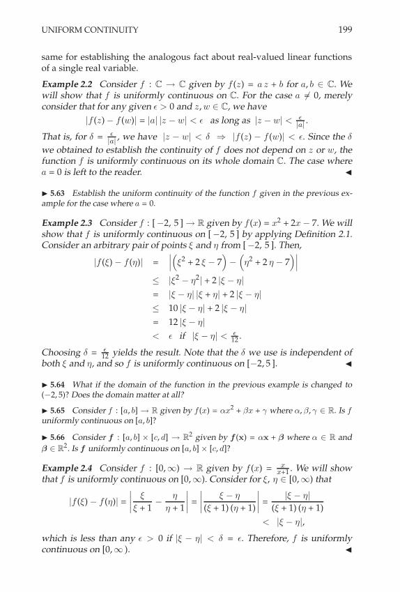
UNIFORM CONTINUITY 199
same for establishing the analogous fact about real-valued linear functionsof a single real variable.
Example 2.2 Consider f : C 3 C given by f (z) = a z + b for a, b # C. Wewill show that f is uniformly continuous on C. For the case a $= 0, merelyconsider that for any given ! > 0 and z, w # C, we have
|f (z) " f (w)| = |a| |z " w| < ! as long as |z " w| < (|a| .
That is, for . = (|a| , we have |z " w| < . ) |f (z) " f (w)| < !. Since the .
we obtained to establish the continuity of f does not depend on z or w, thefunction f is uniformly continuous on its whole domain C. The case wherea = 0 is left to the reader. "
! 5.63 Establish the uniform continuity of the function f given in the previous ex-ample for the case where a = 0.
Example 2.3 Consider f : ["2, 5 ] 3 R given by f (x) = x2 + 2x " 7. We willshow that f is uniformly continuous on ["2, 5 ] by applying Definition 2.1.Consider an arbitrary pair of points ) and , from ["2, 5 ]. Then,
|f ()) " f (,)| =&&&()2 + 2 ) " 7
)"
(,2 + 2 , " 7
)&&&
+ |)2" ,2
| + 2 |) " ,|
= |) " ,| |) + ,| + 2 |) " ,|
+ 10 |) " ,| + 2 |) " ,|
= 12 |) " ,|
< ! if |) " ,| < (12 .
Choosing . = (12 yields the result. Note that the . we use is independent of
both ) and ,, and so f is uniformly continuous on ["2, 5 ]. "
! 5.64 What if the domain of the function in the previous example is changed to(&2, 5)? Does the domain matter at all?
! 5.65 Consider f : [a, b] , R given by f (x) = !x2 + "x + / where !, ", / " R. Is f
uniformly continuous on [a, b]?
! 5.66 Consider f : [a, b] + [c, d] , R2 given by f (x) = !x + " where ! " R and
" " R2. Is f uniformly continuous on [a, b] + [c, d]?
Example 2.4 Consider f : [0,-) 3 R given by f (x) = xx+1 . We will show
that f is uniformly continuous on [0,-). Consider for ), , # [0,-) that
|f ()) " f (,)| =
&&&&)
) + 1"
,
, + 1
&&&& =
&&&&) " ,
() + 1) (, + 1)
&&&& =|) " ,|
() + 1) (, + 1)
< |) " ,|,
which is less than any ! > 0 if |) " ,| < . = !. Therefore, f is uniformlycontinuous on [0,- ). "

200 FUNCTIONS: CONTINUITY AND CONVERGENCE
! 5.67 What if the domain in the previous example is changed to (&1, /)? Is f uni-formly continuous on (&1, /)?
And how does one show that a given continuous function is, in fact, not uni-formly continuous on a given set? We illustrate this in the next example.
Example 2.5 Consider f : (0, 1) 3 R given by f (x) = 1x . As seen in Exam-
ple 1.3 on page 179, this function is continuous on (0,-). However, as indi-cated in that example, the derived . was dependent upon x. We will show,in fact, that f is not uniformly continuous on (0, 1). We will use the methodof proof by contradiction. To this end, assume f is uniformly continuous on(0, 1). Then for ! = 1
2 there exists . > 0 such that
), , # (0, 1) and |) " ,| < . )
&&&&1
)"
1
,
&&&& =|) " ,|
|)| |,|< 1
2 .
With no loss in generality, we may assume that . < 1. (Why?) Note that
the numerator of |!",||!| |,| is restricted in magnitude to be no larger than ., yet
the denominator can be made arbitrarily small (and hence, the overall ratioarbitrarily large) by taking ) and , as close as we like to 0. That is, no matterhow close together ) and , are within (0, 1), we can find such a ) and , as closeto 0 as we need in order to derive the contradiction we seek. In particular,suppose |)",| = +
2 < ., and consider such a ) and , that satisfy 0 < ), , <,
..This yields
|) " ,|
|)| |,|=
./2
) ,>
./2
.= 1
2 ,
a contradiction. Therefore, our initial assumption that f is uniformly contin-uous on (0, 1) cannot be true. "
! 5.68 Answer the (Why?) question in the above example.
! 5.69 Can you change the domain of the function in the last example in such a waythat the resulting function is uniformly continuous on the new domain?
Example 2.6 In this example we will show that f : R 3 R is not uniformlycontinuous on [a,-) for any fixed a # R. To do so, assume the contrary. Thenthere exists . > 0 such that for any ), , # [a,-) satisfying |) " ,| < . we willhave |e!
"e,| < 1. If we choose ) = ,+ +
2 > , > 0, we have that e,++/2"e, < 1
for all , > 0. From this we may write
e,++/2" e, = e,(e+/2
" 1) = e,'+
j=1
(./2)j
j!! e,
,+2
-,
which implies e,,
+2
-< 1 for all , > 0, i.e., e, < 2
+ for all , > 0. This lastis a contradiction. "
! 5.70 Suppose [a, b] ! R. Show that the real exponential function exp : R , R
given by exp(x) = ex is uniformly continuous on [a, b]. Show that it is also uniformly
continuous on (&/, a] for any a " R.

UNIFORM CONTINUITY 201
Example 2.7 Consider f : D23 R given by f (x, y) = 1
x+y , where D2 =
{(x, y) # R2 : x + y ! 1}. We will show that f is uniformly continuous onits domain. To this end, let ! > 0 be given, and consider ! = ()1, )2) and# = (,1, ,2) from D2. Note that
|f (!) " f (#)| =
&&&&1
)1 + )2"
1
,1 + ,2
&&&& =|(,1 " )1) + (,2 " )2)|
()1 + )2) (,1 + ,2)
+ |,1 " )1| + |,2 " )2|
+ |# " !| + |# " !|
= 2 |# " !|
< ! if |# " !| < (2 .
Therefore, choosing . /(2 establishes the result. "
2.2 Topological Properties and Consequences
Interestingly enough, what can often determine the uniform continuity of acontinuous function on a certain set are the topological characteristics of theset, rather than any particular qualities the function possesses. The examplesand exercises up to this point might have already led the reader to suspectthis very idea. The following theorem points out how compactness of the setin question plays the key role in this issue.
Theorem 2.8 Suppose f : D 3 Y is continuous on a compact set K ' D. Then fis uniformly continuous on K .
PROOF Suppose ! > 0 is given. For each x0 # K there exists a .x0 > 0 suchthat
x # K and |x " x0| < .x0 ) |f (x) " f (x0)| < (2 ,
i.e., we have thatx #
,K & N+x0
(x0)-
) |f (x) " f (x0)| < (2 .
Here, .x0 emphasizes the potential dependence of . on x0. Of course, we willshow in this case that the dependence does not, in fact, exist. It is certainlytrue that for each x0 # K we have x0 # N 1
2 +x0(x0), and so it follows that
K '
?
x#K
N 12 +x
(x).
But since K is compact, there exists a finite collection x1, x2, . . . , xm # Ksuch that
K '
m?
j=1
N 12+xj
(xj ).
Now choose. / min
,12.x1 , 1
2.x2 . . . , 12.xm
-, (5.5)
and consider any pair of points ), , # K such that |) " ,| < .. Since ) #

202 FUNCTIONS: CONTINUITY AND CONVERGENCE
N 12 +xj%
(xj)) for some j< # {1, 2, . . . , m}, we know that |) " xj)| < 12.xj% . But
we also know that|, " xj)| + |, " )| + |) " xj)| < . + 1
2.xj% < .xj% ,
and so ) and , both belong to N+xj%(xj)). This means that
|f ()) " f (xj))| < (2 and |f (,) " f (xj))| < (
2 .
From this we obtain
|f ()) " f (,)| + |f ()) " f (xj))| + |f (xj)) " f (,)| < !.
That is, for . > 0 chosen according to (5.5), we have that
), , # K and |) " ,| < . ) |f ()) " f (,)| < !,
and the theorem is proved. #
Example 2.9 Consider f : [0, 1] 3 R given by
f (x) =
Ex sin 1
x for 0 < x + 1
0 for x = 0.
We will show that f is uniformly continuous on [0, 1]. Since [0, 1] is compact,by Theorem 2.8, we only need to show that f is continuous on [0, 1]. Thefunction f is clearly continuous on (0, 1], and so we need only show that it isalso continuous at x0 = 0. To see this, consider
&&&x sin 1x " 0
&&& = |x|&&&sin 1
x
&&& + |x| < ! if |x| < . = !.
Hence, f is continuous at x0 = 0, and therefore on all of [0, 1]. By Theorem 2.8,f is uniformly continuous on [0, 1]. "
! 5.71 Fix ! " R and consider the function f : [0, 1] , R given by
f (x) =
Ex
! sin 1x
for 0 < x # 1
0 for x = 0.
For what values of ! is the function uniformly continuous on [0, 1]?
Consequences of Uniform Continuity
There are some significant consequences of a function being uniformly con-tinuous on its domain. Our first result establishes that uniform continuitypreserves the Cauchy property.
Proposition 2.10 Suppose f : D 3 Y is uniformly continuous on D. If {xn} is aCauchy sequence in D, then {f (xn)} is a Cauchy sequence in Y.

UNIFORM CONTINUITY 203
PROOF Assume f is uniformly continuous on D. Then given ! > 0, thereexists . > 0 such that
), , # D and |) " ,| < . ) |f ()) " f (,)| < !. (5.6)
Since {xn} is Cauchy, there exists N # N such that
n, m > N ) |xn " xm| < .. (5.7)
Combining expressions (5.6) and (5.7) yields
n, m > N ) |f (xn) " f (xm)| < !,
and the result is proved. #
! 5.72 What happens if in the statement of the above proposition, you replace uni-form continuity with mere continuity?
The following proposition establishes the fact that a uniformly continuousfunction “preserves boundedness.”
Proposition 2.11 If D ' X is bounded and f : D 3 Y is uniformly continuouson D, then f (D) is bounded.
PROOF Since f is uniformly continuous on D there exists . > 0 such that
), , # D and |) " ,| < . ) |f ()) " f (,)| < 1.
Assume that f is not bounded on D. Then there exists a sequence {xn} '
D such that |f (xn)| ! n for all integers n ! 1. Since the sequence {xn} isbounded, there exists a convergent subsequence {xnm} with the propertythat limm(' xnm = x0 for some x0 # D. Therefore the deleted neighborhoodN &
"2
(x0) contains xj for infinitely many values of j. Fix one of these points,
say, xJ . Then it follows that |xj " xJ | < . for infinitely many values of j,which in turn implies that |f (xj)"f (xJ )| < 1, and hence, |f (xj )| < 1 + |f (xJ )|for infinitely many values of j. But this is a contradiction, since |f (xj)| ! jfor all j. Therefore, f must be bounded on D. #
Recall that the function f : (0, 1) 3 R given by f (x) = 1x maps its bounded
domain to (1,-), an unbounded range. Therefore by the above proposition,we may conclude that f cannot be uniformly continuous on its domain.
! 5.73 Suppose f : D , R is uniformly continuous on D. If D is not bounded, whatcan you say about f (D)? What if D is bounded, but f is merely continuous?
2.3 Continuous Extensions
Recall that in the case of a removable discontinuity at x0 # D1' R, a function
f : D13 R that is continuous on D1
\ {x0} can be “redefined” at x0 so as

204 FUNCTIONS: CONTINUITY AND CONVERGENCE
to be continuous on all of D1. We now consider a slightly different problem.Stated generally, suppose f : D 3 Y possesses certain properties throughoutits domain D, but one would like to “extend” the function so as to possessthem at points beyond D. Such extensions are not always possible in general.In this subsection, we will consider the more specific problem of how onemight extend a continuous function f : D 3 Y to a continuous functionGf : B 9 D 3 Y, such that Gf = f on D. We refer to Gf as a continuous extension off , and we say that f has been continuously extended to B. As we will see, thisparticular type of extension is not always possible either, unless the domainD is closed. We begin with a simple example.
Example 2.12 Consider f : (0, 1) 3 R given by f (x) = x2. Clearly, f iscontinuous on its specified domain. Perhaps one would like to extend fto a larger set, say ("2, 2). One might also wish, along with the extensionequalling f on (0, 1), that it be continuous throughout ("2, 2). One obvi-
ous way to accomplish this is with the function Gf1 : ("2, 2) 3 R given byGf1(x) = x2. If we also require that the extension be bounded by the samebounds that applied to the original function f , where 0 + |f (x)| + 1 for allx # (0, 1), then this particular extension won’t do. However, a continuousextension that satisfies this additional requirement is given by the functionGf2 : ("2, 2) 3 R defined as
Gf2(x) =
RST
SU
0 if "2 < x + 0,
x2 if 0 < x < 1,
1 if 1 + x < 2.
The reader can verify that Gf2 = f on (0, 1), that Gf2 is continuous throughout("2, 2), and that 0 +
&& Gf2(x)&&+ 1 for all x # ("2, 2). "
While the above example illustrates that what we wish to do may be possi-ble, it makes no claim as to the uniqueness of the extensions presented. Theremay be many ways to extend a given function to larger domains while retain-ing certain specified properties of the original function. While such questionsof uniqueness can ultimately be of interest, it is first useful to know whensuch continuous extensions exist. The following theorem, called the pastingtheorem, gives sufficient conditions for the existence of such an extension.
Theorem 2.13 (The Pasting Theorem)Suppose D = A % B where A and B are closed subsets of D. Let f : A 3 Y andg : B 3 Y be continuous functions. If f (x) = g(x) for all x # A & B, then f and gextend to the continuous function h : D = A % B 3 R given by
h(x) =
Ef (x) if x # A,
g(x) if x # B.
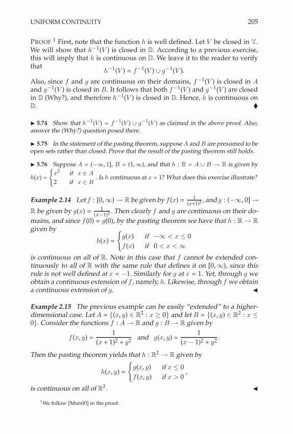
UNIFORM CONTINUITY 205
PROOF 1 First, note that the function h is well defined. Let V be closed in Y.We will show that h"1(V ) is closed in D. According to a previous exercise,this will imply that h is continuous on D. We leave it to the reader to verifythat
h"1(V ) = f"1(V ) % g"1(V ).
Also, since f and g are continuous on their domains, f"1(V ) is closed in Aand g"1(V ) is closed in B. It follows that both f"1(V ) and g"1(V ) are closedin D (Why?), and therefore h"1(V ) is closed in D. Hence, h is continuous onD. #
! 5.74 Show that h!1(V ) = f
!1(V ) 0 g!1(V ) as claimed in the above proof. Also,
answer the (Why?) question posed there.
! 5.75 In the statement of the pasting theorem, suppose A and B are presumed to beopen sets rather than closed. Prove that the result of the pasting theorem still holds.
! 5.76 Suppose A = (&/, 1], B = (1, /), and that h : R = A 0 B , R is given by
h(x) =
Ex
2 if x " A
2 if x " B. Is h continuous at x = 1? What does this exercise illustrate?
Example 2.14 Let f : [0,-) 3 R be given by f (x) = 1(x+1)2 , and g : ("-, 0] 3
R be given by g(x) = 1(x"1)2 . Then clearly f and g are continuous on their do-
mains, and since f (0) = g(0), by the pasting theorem we have that h : R 3 R
given by
h(x) =
Eg(x) if "- < x + 0
f (x) if 0 < x < -
is continuous on all of R. Note in this case that f cannot be extended con-tinuously to all of R with the same rule that defines it on [0,-), since thisrule is not well defined at x = "1. Similarly for g at x = 1. Yet, through g weobtain a continuous extension of f , namely, h. Likewise, through f we obtaina continuous extension of g. "
Example 2.15 The previous example can be easily “extended” to a higher-dimensional case. Let A = {(x, y) # R2 : x ! 0} and let B = {(x, y) # R2 : x +
0}. Consider the functions f : A 3 R and g : B 3 R given by
f (x, y) =1
(x + 1)2 + y2and g(x, y) =
1
(x " 1)2 + y2.
Then the pasting theorem yields that h : R23 R given by
h(x, y) =
Eg(x, y) if x + 0
f (x, y) if x > 0,
is continuous on all of R2. "
1We follow [Mun00] in the proof.
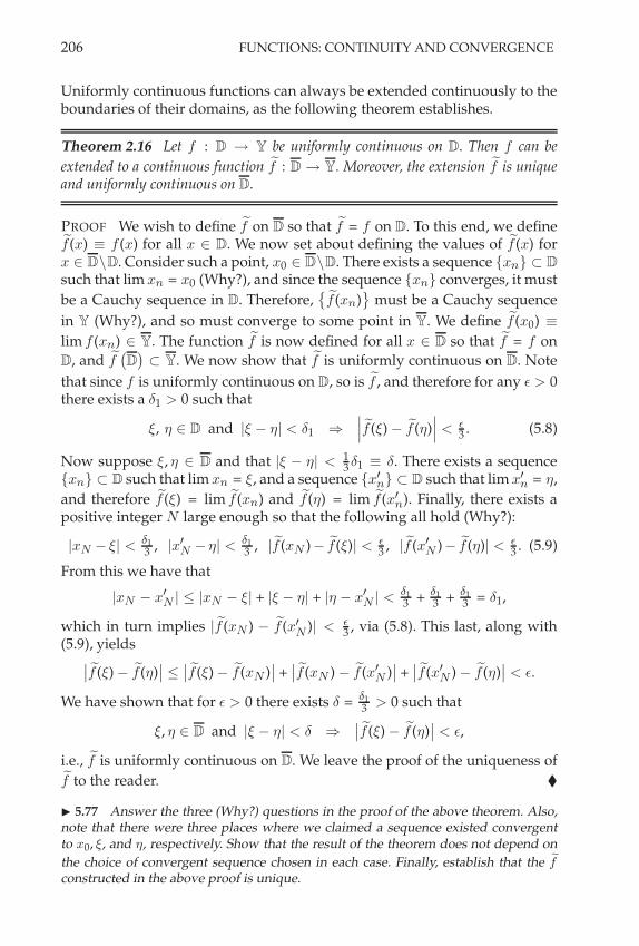
206 FUNCTIONS: CONTINUITY AND CONVERGENCE
Uniformly continuous functions can always be extended continuously to theboundaries of their domains, as the following theorem establishes.
Theorem 2.16 Let f : D 3 Y be uniformly continuous on D. Then f can be
extended to a continuous function Gf : D 3 Y. Moreover, the extension Gf is uniqueand uniformly continuous on D.
PROOF We wish to define Gf on D so that Gf = f on D. To this end, we defineGf (x) / f (x) for all x # D. We now set about defining the values of Gf (x) forx # D\D. Consider such a point, x0 # D\D. There exists a sequence {xn} ' D
such that lim xn = x0 (Why?), and since the sequence {xn} converges, it must
be a Cauchy sequence in D. Therefore,. Gf (xn)
/must be a Cauchy sequence
in Y (Why?), and so must converge to some point in Y. We define Gf (x0) /
lim f (xn) # Y. The function Gf is now defined for all x # D so that Gf = f onD, and Gf
,D-' Y. We now show that Gf is uniformly continuous on D. Note
that since f is uniformly continuous on D, so is Gf , and therefore for any ! > 0there exists a .1 > 0 such that
), , # D and |) " ,| < .1 )
&&& Gf ()) " Gf (,)&&& < (
3 . (5.8)
Now suppose ), , # D and that |) " ,| < 13.1 / .. There exists a sequence
{xn} ' D such that lim xn = ), and a sequence {x&n} ' D such that lim x&n = ,,
and therefore Gf ()) = lim Gf (xn) and Gf (,) = lim Gf (x&n). Finally, there exists apositive integer N large enough so that the following all hold (Why?):
|xN " )| < +13 , |x&N " ,| < +1
3 , |Gf (xN )" Gf ())| < (
3 , |Gf (x&N )" Gf (,)| < (
3 . (5.9)
From this we have that
|xN " x&N | + |xN " )| + |) " ,| + |, " x&N | < +13 + +1
3 + +13 = .1,
which in turn implies |Gf (xN ) " Gf (x&N )| < (
3 , via (5.8). This last, along with(5.9), yields
&& Gf ()) " Gf (,)&&+
&& Gf ()) " Gf (xN )&& +
&& Gf (xN ) " Gf (x&N )&& +
&& Gf (x&N ) " Gf (,)&& < !.
We have shown that for ! > 0 there exists . = +13 > 0 such that
), , # D and |) " ,| < . )
&& Gf ()) " Gf (,)&& < !,
i.e., Gf is uniformly continuous on D. We leave the proof of the uniqueness ofGf to the reader. #
! 5.77 Answer the three (Why?) questions in the proof of the above theorem. Also,note that there were three places where we claimed a sequence existed convergentto x0, #, and ), respectively. Show that the result of the theorem does not depend on
the choice of convergent sequence chosen in each case. Finally, establish that the Gfconstructed in the above proof is unique.

UNIFORM CONTINUITY 207
Note that the function f : (0, 1) 3 R given by f (x) = 1x is continuous on
(0, 1). However, there is no way to extend f continuously to x0 = 0 sincelimx(0+ f (x) = -. In fact, the sequence {xn} ' (0, 1) with xn = 1
n for n # N
is such that lim xn = 0, but lim f (xn) does not exist. This example shows thatnot all continuous functions can be extended continuously to the boundaryof their domains. The key in this case is that the function f is not uniformlycontinuous on (0, 1). This example points to the following result, the proof ofwhich is left to the reader.
Proposition 2.17 Suppose f : D 3 Y is continuous on the bounded domain D.Then f can be extended continuously to the closure D if and only if f is uniformlycontinuous on D.
! 5.78 Prove the above proposition.
Recall that the function Arg(z) was defined on C\{0} and that it is continuousonly on C \ K where K = {z # C : Re(z) + 0, Im(z) = 0} . In the followingexample, we establish that the restriction to C \ K of the function Arg(z)cannot be extended continuously to all of C, or even to C \ {0}.
Example 2.18 Consider the function f : C \ K 3 R given by f (z) = Arg(z).We will show that f (z) cannot be continuously extended to all of C \ {0}. To
this end, suppose there exists such an extension, Gf : C \ {0} 3 C, continuouson C \ {0} such that Gf (z) = Arg(z) for all z # C \ K . We will derive a contra-
diction. Consider the sequence of points {zn} with zn = ei ($" 1n ) for n # N.
These points approach z = "1 from above the real axis along the the arc of
the unit circle centered at the origin. Since lim zn = "1, continuity of Gf on Kimplies
Gf ("1) = Gf (lim zn) = lim Gf (zn) = lim Arg(zn) = lim(% "1n ) = %. (5.10)
If we now consider the points {wn} with wn = ei ("$+ 1n ) for n # N, a sequence
approaching z = "1 from below the real axis along the arc of the unit circlecentered at the origin, then clearly lim wn = "1. However, by the continuityof Gf on K we now conclude that
Gf ("1) = Gf (lim wn) = lim Gf (wn) = lim Arg(wn) = lim("% + 1
n
)= "%.
This contradicts (5.10). "
! 5.79 Is f : C \ {0} , R given by f (z) = Arg(z) uniformly continuous on C \ K?
! 5.80 What are the implications of the previous example as it relates to the func-
tions Log(z) and z1/2?
Another significant continuous extension result is the Tietze extension theo-rem. It states that if D is closed, and if f : D 3 Y is continuous and bounded

208 FUNCTIONS: CONTINUITY AND CONVERGENCE
on D, i.e., |f | + M , then f can be extended to a continuous function on thewhole space X 9 D such that the extension is also bounded by M . To estab-lish this result requires the use of sequences and series of functions, topicswe develop next.
3 SEQUENCES AND SERIES OF FUNCTIONS
In this section we broaden our concept of sequences to include sequences offunctions. This is a more sophisticated notion than a mere sequence of num-bers, or even of vectors. One can develop the same intuitive understandingthat the geometry of convergence of points allows, and some texts do so. Inthis view, one considers functions as points in a function space, and a se-quence of functions is considered to converge if these points are determinedto be getting closer to a well-defined limit function in that space. We choosenot to pursue this point of view in our treatment of analysis, as it requiresdevelopment of the more abstract notion of a metric space. In choosing a lesssophisticated approach, we remind the reader that functions are more com-plicated mathematical objects than mere numbers or vectors.
3.1 Definitions and Examples
Definition 3.1 Consider fn : D 3 Y for n = 1, 2, . . . . We call the collec-tion {fn} a sequence of functions. We say the sequence is convergent andwe write limn(' fn(x) = f (x), where f is called the limit function of thesequence, if both of the following are true:
1. The limit function has the same domain and codomain as thefunctions in the sequence. That is, f : D 3 Y.
2. For each ! > 0 and each x0 # D, there exists an N # N suchthat n > N ) |fn(x0) " f (x0)| < !.
It is worth noting that the N referred to in Definition 3.1 will generally de-pend on both ! and x0. In the special case where N does not depend on x0,the convergence is rather special. Also, the definition of convergence givenabove is sometimes more specifically referred to as “pointwise convergence”to distinguish it from other, more subtle modes of convergence that might bedefined for sequences of functions. The term “pointwise” refers to the factthat the sequence of functions must converge to the limit function at everypoint in the domain. While interesting, and of great use in more advancedtopics in analysis, we won’t have need of any of the other types of conver-gence in what follows. For this reason, our use of the unadorned term “con-vergence” will always mean “pointwise convergence.”

SEQUENCES AND SERIES OF FUNCTIONS 209
An alternative version of condition 2 in the above definition of convergenceis the following equivalent statement:
2&. For each x0 # D, the sequence of points {fn(x0)} # Y convergesto the point f (x0) # Y. That is,
x0 # D ) limn(' fn(x0) = f (x0).
Example 3.2 Consider the functions fn : ("1, 1) 3 R given by fn(x) = xn
for n # N, and let f : ("1, 1) 3 R be given by f (x) / 0. We will show thatlimn(' fn(x) = f (x) = 0 on ("1, 1). To this end, fix an arbitrary x0 # ("1, 1).Then,
|fn(x0) " f (x0)| = |xn0 | = |x0|
n.
Certainly the above expression will be less than any given ! > 0 for x0 = 0. Inthe case x0 $= 0 the expression will be less than any given ! > 0 as long as n >
ln (ln |x0|
. That is, for any ! > 0 and any specified x0 # ("1, 1), we choose N # N
such that N > ln (ln |x0|
. We then have that n > N ) |fn(x0) " f (x0)| < !, i.e.,
limn(' fn(x0) = f (x0). "
Note in the previous example that the value of N that fulfills our definitionof convergence, Definition 3.1, depends on x0.
! 5.81 Consider the sequence of complex functions fn : N1(0) , C described byfn(z) = z
n for n " N, and the complex function f : N1(0) , C given by f (z) . 0 onN1(0) ! C. What can you say about limn&% fn(z) on N1(0)?
We consider another example.
Example 3.3 Let D2 = {x = (x, y) # R2 : |x| < 1}, and consider the functionsfn : D2
3 R2 given byfn(x) =
(xn,
n y
n + 1
).
We outline the argument for showing that limn(' fn(x) = (0, y) / f (x), andleave the details to the reader. We denote fn(x) component-wise by fn(x) =(f1n(x, y), f2n(x, y)), and we proceed to examine the component functionsf1n(x, y) = xn and f2n(x, y) = n y
n+1 for fixed values of x and y. One only needsto show that for all (x, y) # D2, limn(' f1n(x, y) = 0, and limn(' f2n(x, y) =y to determine the limit limn(' fn(x). "
! 5.82 Complete the argument of the last example. Does the N required to establishconvergence depend on x and/or y, and hence on (x, y) = x?
! 5.83 Let fn : [0, 1] , R be given by fn(x) = xn for n " N. Use the Definition 3.1 to
show that limn&%
fn(x) =
$0 for 0 # x < 11 for x = 1
. Does the N required depend on x?
Note that each fn is continuous on [0, 1], but the limit function f is not.
! 5.84 Consider the sequence of functions fn : R , R given by fn(x) = sin(nx)"n
for
n " N. Find limn&% fn(x).
! 5.85 For D = {z " C : Re(z) %= 0}, consider the sequence of functions fn : D , C
given by fn(z) = e!nz for n " N. Find limn&% fn(z).

210 FUNCTIONS: CONTINUITY AND CONVERGENCE
3.2 Uniform Convergence
We now define a special form of convergence for a sequence of functions,a form that carries with it some rather important implications. Recall thatuniform continuity implied more about a function’s behavior than regularcontinuity. Likewise, we will find that uniform convergence implies more abouta sequence’s behavior than regular convergence. We begin with a definition.
Definition 3.4 Let {fn} be a sequence of functions, each with domain D andcodomain Y, that converges to the limit function f according to Definition 3.1on page 208. We will say that the convergence is uniform on D, or that thesequence converges uniformly on D if the following is true:
For each ! > 0, there exists an N # N such that for all x0 # D,n > N ) |fn(x0) " f (x0)| < !.
It is worth emphasizing how uniform convergence differs from ordinary con-vergence. In comparing Definition 3.1 on page 208 with the definition of uni-form convergence given above, one should note that uniform convergencehas the added condition that the value of N required to satisfy the definitionmust be independent of x0 # D. This difference will be seen to have significantimplications.
Example 3.5 Recall our sequence of functions from Example 3.2, namely,fn : ("1, 1) 3 R given by fn(x) = xn for n ! 1. In that example, we showedthat lim fn(x) = 0 on ("1, 1). While we alluded to the convergence beingnonuniform, we now show this to be the case unequivocally. To show this,let’s assume otherwise. That is, assume there exists an N # N such that forany x # ("1, 1),
n > N ) |xn" 0| < 1
2 .
Note that we have chosen the ! value to be 12 here for convenience. The defini-
tion for convergence must be true for any positive !, so certainly it must alsobe true for this particular choice. From the above mentioned assumption, wemay conclude that &&xN+1
&& < 12 for all x # ("1, 1).
Taking the left-handed limit as x approaches 1 on each side of the aboveinequality yields
limx(1"
&&&xN+1&&& = 1 +
12 ,
a contradiction. Hence, our initial assumption that the convergence is uni-form on ("1, 1) is incorrect. "
Example 3.6 Fix 0 < a < 1 and consider the functions fn : ["a, a] 3 R
given by fn(x) = xn for n ! 1. We will show that in this case, with the domainof definition for each fn altered from the previous example, the convergenceof limn(' fn(x) = f (x) / 0 is uniform on ["a, a]. To establish this, note

SEQUENCES AND SERIES OF FUNCTIONS 211
that for any x # ["a, a] we have that |xn" 0| = |x|n. Clearly, for any given
! > 0 we have |x|n < ! for any n when x = 0. Also, for any x # ["a, a]we have |x|n + an, and this will be less than any given ! as long as n > ln (
ln a .Clearly neither case requires an N that depends on x, and so the convergenceis uniform as claimed. "
Example 3.7 Consider the functions fn : D 3 C for n # N and D = {z #
C : |z| + 1} given by fn(z) = n z2
n+1+z . We will show that the sequence {fn}
converges uniformly to some limit function f : D 3 C. In fact, it is easy tosee that
lim fn(z) = lim
2z2
1 + 1n + z
n
3= z2 = f (z) on D.
To show that the convergence is uniform, note that
|fn(z) " f (z)| =
&&&&n z2
n + 1 + z" z2
&&&& =|z2 + z3
|
|n + 1 + z|+
|z|2 + |z|3
n + 1 " |z|+
2n+1"1 = 2
n .
Clearly, given any ! > 0 the above will be less than ! if n > 2( . Therefore, the
convergence is uniform on D. "
There are many interesting consequences of uniform convergence that wewill explore in later chapters. For now, we satisfy ourselves with one of thesimpler ones, namely, the preservation of continuity.
Theorem 3.8 Suppose {fn} is a sequence of continuous functions on D where fn :D 3 Y for each n = 1, 2, . . . . If {fn} converges uniformly to f on D, then f is alsocontinuous on D.
PROOF For any ! > 0 there exists N # N such that for all x # D,
n > N ) |fn(x) " f (x)| < (3 . (5.11)
Fix M > N . Then, |fM (x)" f (x)| < (3 for all x # D. Now fix x0 # D. Since fM
is continuous at x0, there exists a . > 0 such that
x # D and |x " x0| < . ) |fM (x) " fM (x0)| < (3 . (5.12)
Combining inequalities (5.11) and (5.12), we obtain that x # D and |x"x0| <. together imply
|f (x) " f (x0)| = |f (x) " fM (x) + fM (x) " fM (x0) + fM (x0) " f (x0)|
+ |f (x) " fM (x)| + |fM (x) " fM (x0)| + |fM (x0) " f (x0)|
< (3 + (
3 + (3 = !,
and so f is continuous at x0. #
! 5.86 In a previous exercise, we saw that fn : [0, 1] , R given by fn(x) = xn for
n " N converged to f (x) =
E0 for 0 # x < 1
1 for x = 1. Is the convergence uniform?
212 FUNCTIONS: CONTINUITY AND CONVERGENCE
! 5.87 Let fn : (0, 1] , R be given by fn(x) =
E1 for 0 < x # 1
n
0 for 1n
< x # 1.Note that
the functions {fn} are not continuous on (0, 1]. Show that the limit function f (x) .lim fn(x) is continuous on (0, 1], and the convergence is not uniform. What does thissay about Theorem 3.8?
There is an important consequence following from the above theorem. Sup-pose {fn(x)} is a sequence of continuous functions on D that converges uni-formly to f (x) on D. If x0 is a limit point of D, it can be shown that
limx(x0
limn('
fn(x) = limn('
limx(x0
fn(x), (5.13)
i.e., the two limits may be interchanged. Such limit interchanges can be con-venient.
! 5.88 Prove the equality (5.13) under the conditions described above.
Criteria for Uniform Convergence
The notion of a Cauchy sequence is relevant for sequences of functions justas it is for sequences of vectors. In particular, we define what it means for asequence of functions {fn} to be uniformly Cauchy on their common domain.
Definition 3.9 Suppose {fn} is a sequence of functions where fn : D 3 Y.We say the sequence is uniformly Cauchy on D if for each ! > 0 there existsan N # N such that
m, n > N ) |fn(x) " fm(x)| < ! for all x # D.
Note that the N that corresponds to a given ! in the above definition is in-dependent of x # D. This is the “uniform” part of the definition of uniformlyCauchy.
The following proposition establishes the important fact that, under certainconditions, the sequence {fn} converges uniformly to a function f : D 3 Y
if and only if the convergence is uniformly Cauchy on D.
Proposition 3.10 Suppose {fn} is a sequence of functions where fn : D 3 Y andY is R, Rp, or C for all of n = 1, 2, . . . . Then {fn} converges uniformly to a functionf : D 3 Y if and only if the convergence is uniformly Cauchy on D.
The key point here is that Y be complete, as the proof will show.
PROOF Suppose {fn} converges uniformly to f on D, and let ! > 0 be given.Then there exists an N # N such that
n > N and x # D ) |fn(x) " f (x)| < (2 .
Similarly,

SEQUENCES AND SERIES OF FUNCTIONS 213
m > N and x # D ) |fm(x) " f (x)| < (2 .
Therefore, m, n > N and x # D implies that, for all x # D,
|fn(x) " fm(x)| = |fn(x) " f (x) + f (x) " fm(x)|
+ |fn(x) " f (x)| + |f (x) " fm(x)|
< (2 + (
2 = !.
Hence, the convergence is uniformly Cauchy on D. Suppose now that {fn}
is a sequence of functions from D to Y with the property that for each ! > 0there exists an N # N such that
m, n > N and x # D ) |fn(x) " fm(x)| < !. (5.14)
We will show that limn(' fn(x) = f (x) exists, and the convergence is uni-form. To this end, note that according to (5.14), for any fixed x # D the se-quence {fn(x)} is a Cauchy sequence of elements in Y. Therefore, since Y
is complete, limn(' fn(x) = f (x) exists. To prove that the convergence isuniform, let ! > 0 be given. Then there exists an N # N such that
m, n > N and x # D ) |fn(x) " fm(x)| < (2 .
Now fix n > N and x # D, and take the limit as m 3 - on each side of thelast inequality. This yields
n > N and x # D ) |fn(x) " f (x)| + (2 < !. (5.15)
Since the N in expression (5.15) does not depend on x, the proposition isproved. #
! 5.89 Suppose in the statement of the previous proposition that Y is presumed tobe a subset of R, R
p, or C. In this case, what else must be presumed about Y in orderfor the argument given in the above proof to remain valid?
! 5.90 Consider the sequence of functions fn : [&a, a ] , R given by fn(x) = xn
where 0 # a < 1. Establish that the sequence {fn} is uniformly Cauchy on [&a, a ],first by applying Proposition 3.10, and then by applying Definition 3.9. Which methodis easier?
Proposition 3.10 is a nice result in that, when Y is complete it character-izes uniformly convergent sequences of functions as those that have the uni-formly Cauchy property. This has great value, particularly in proving theo-rems where it is not always necessary to know, or even possible to determine,the exact form of the limit function. Just confirming that the sequence con-verges uniformly to some limit function is often enough. For example, if eachfn is continuous and {fn} is a uniformly Cauchy sequence, Proposition 3.10implies that fn converges to some function f uniformly. Theorem 3.8 thenimplies that the limit function f is continuous, even if it’s not possible tocharacterize its explicit form.

214 FUNCTIONS: CONTINUITY AND CONVERGENCE
Example 3.11 Consider a sequence of complex functions fn : D 3 C suchthat for all n # N and for all z # D,
|fn+1(z) " fn(z)| < c rn, where c # R and 0 < r < 1.
We will show that {fn} is uniformly Cauchy on D, and hence converges uni-formly to some function f : D 3 C. To this end, if n > m we have
|fn(z) " fm(z)| + |fn(z) " fn"1(z)| + |fn"1(z) " fn"2(z)| + · · ·
+ |fm+1(z) " fm(z)|
< c rn"1 + c rn"2 + · · · + c rm
< c rm(
1 + r + r2 + · · ·
)
=c rm
1 " r.
In general, we then have that
|fn(z) " fm(z)| +c rmin(m,n)
1 " r,
and the last expression above will be less than ! if m, n > N for some N #
N. (Why?) Therefore {fn} is uniformly Cauchy on D and hence convergesuniformly to some limit function f : D 3 C. "
! 5.91 Answer the (Why?) question in the above example. Also, come up with an ex-plicit example of a sequence of complex functions fn : D , C behaving as describedthere. Do the functions fn have to be complex functions?
In fact, when dealing with sequences of functions it is often not possible tocharacterize the form of the limit function, even in cases where the conver-gence is uniform. If one does know the limiting function, a situation that isrelatively rare, the following result provides a convenient test for determin-ing whether the convergence is uniform. The test is easy to use because itrelates the convergence of functions to the convergence of real numbers.
Theorem 3.12 (The M-Test)Suppose {fn} is a sequence of functions where fn : D 3 Y for each n = 1, 2, . . . ,that f : D 3 Y, and that limn(' fn(x) = f (x) for all x # D. Suppose too thatMn / supx#D
|fn(x) " f (x)| exists for all n. Then {fn} converges uniformly to fon D if and only if lim Mn = 0.
PROOF Suppose lim Mn = 0, and let ! > 0 be given. Then there exists anN # N such that n > N ) Mn < !. Note that this N is independent of anyx # D. With this same N we also have that
n > N ) |fn(x) " f (x)| + Mn < !,
and so the sequence {fn} converges to f uniformly. Conversely, suppose

SEQUENCES AND SERIES OF FUNCTIONS 215
limn(' fn(x) = f (x) uniformly on D, and let ! > 0 be given. Then thereexists an N # N such that
n > N and x # D ) |fn(x) " f (x)| < (2 . (5.16)
Since N in expression (5.16) is independent of x # D, we clearly have
n > N ) Mn = supx#D
|fn(x) " f (x)| + (2 < !.
Hence, lim Mn = 0 and the theorem is proved. #
The M-test says, roughly, that for a sequence of functions {fn} convergingto f on D, the convergence will be uniform on D exactly when the biggestdifference in values between fn(x) and f (x) over D goes to 0 as n goes to -.
Example 3.13 Let fn : [0, 1] 3 R be given by fn(x) = xn for n # N. Note that
limn('
fn(x) = f (x) =
E0 for 0 + x < 1
1 for x = 1,
and that Mn = supx#[0,1] |fn(x) " f (x)| = 1. Since lim Mn $= 0, it follows fromthe M-test that the convergence is not uniform on [0, 1]. "
Example 3.14 Let fn : D 3 C be given by fn(z) = zn for n # N, whereD = Na(0) for 0 < a < 1. Then limn(' fn(z) = 0 (Why?), and
Mn = supz#D
|zn| = sup
z#D
|z|n = an.
Since lim Mn = 0, it follows by the M-test that the convergence is uniform onD. "
! 5.92 Answer the (Why?) question in the last example.
Example 3.15 Let fn : [1, 2] 3 R be given by fn(x) = n2x1+n3x2 for n # N. Then
limn(' fn(x) = 0 on [1, 2], and the convergence is uniform on [1, 2]. To seethis, note that
Mn = sup[1,2]
&& n2x1+n3x2
&& = max[1,2]
,n2x
1+n3x2
-.
To evaluate Mn, it is not difficult to show that for n fixed, fn(x) = n2x1+n3x2 is
decreasing on [1, 2], and therefore Mn = n2
1+n3 . Clearly then, lim Mn = 0. "
! 5.93 Show that fn(x) = n2x
1+n3x2 is decreasing on [1, 2].
! 5.94 Let fn : D , C be given by fn(z) = n2z
1+n3z2 for n = 2, 3, . . ., where D = {z "C : 1 # |z| # 2}. Find f (z) = lim fn(z). Is the convergence uniform on D?
Example 3.16 Let fn be given by fn(x) = n2x1+n3x2 for n # N as in the previ-
ous example, but change the domain to [0, 1]. We will show that although
216 FUNCTIONS: CONTINUITY AND CONVERGENCE
limn(' fn(x) = 0 as before, the convergence is not uniform on [0, 1]. To seethis, note that
Mn = sup[0,1]
&& n2x1+n3x2
&& = max[0,1]
,n2x
1+n3x2
-,
butMn !
n2(
1n3/2
)
1 + n3(
1n3/2
)2 =
,
n
2.
Therefore, lim Mn $= 0, and so the convergence is not uniform on [0, 1]. "
3.3 Series of Functions
Just as we generalized the notion of sequences to sequences of functions, wecan also generalize the notion of series to series of functions. We begin witha definition.
Definition 3.17 Let fj : D 3 Y for j # N be a sequence of functions.
1. The series;'
j=1 fj(x) is referred to as the series of functions
associated with the sequence {fj}.
2. The function sn : D 3 Y for each n # N, defined by
sn(x) /;n
j=1 fj(x), is called the nth partial sum of the series,
and the sequence of functions {sn} is called the sequence of
partial sums associated with the series;'
j=1 fj (x).
Of course, we are primarily concerned with those series of functions thatconverge in some sense. We define this concept next.
Definition 3.18 Suppose;'
j=1 fj(x) is a series of functions fj : D 3 Y forj # N, with the associated sequence of partial sums {sn}. If the sequence{sn} converges on D to some function s : D 3 Y, then we say that the series;'
j=1 fj(x) converges to the function s : D 3 Y, and we write
s(x) ='+
j=1
fj(x) for each x # D.
Example 3.19 Let fj : ("1, 1) 3 R be given by fj(x) = xj for j ! 0. Then,;'j=0 fj(x) is a geometric series with ratio x, and so
'+
j=0
fj (x) ='+
j=0
xj =1
1 " x= s(x) for |x| < 1, i.e., on ("1, 1).
"
Example 3.20 Consider the series of complex functions given by;'
j=0
(4z
)j.
Since this is a geometric series with ratio 4z , we may conclude that the series

SEQUENCES AND SERIES OF FUNCTIONS 217
converges to s(z) / 11" 4
z
= zz"4 if
&&& 4z
&&& < 1. That is, the series converges to the
function s(z) = zz"4 on |z| > 4. "
! 5.95 What if the series in the previous example is replaced by;%
j=0
,z0z
-j, for
some z0 " C? On what part of the complex plane is the series convergent now?
Just as with sequences of functions, series of functions can converge uni-formly. We specify this idea next.
Definition 3.21 Let fj : D 3 Y for j # N be a sequence of functions, andsuppose the series
;'j=1 fj(x) converges to the function s : D 3 Y. We say
that the series converges uniformly on D if the sequence of associated partialsums {sn} converges uniformly to s on D.
Example 3.22 Consider again the functions fj : ("1, 1) 3 R given by fj(x) =xj for j ! 0. We learned in Example 3.19 above that
'+
j=0
fj(x) ='+
j=0
xj =1
1 " x= s(x) on ("1, 1).
So certainly the series also converges to s(x) on ["a, a] ' ("1, 1). In fact, theconvergence on such an interval ["a, a] is uniform. To see this, consider
sn(x) =n+
j=1
xj =1 " xn+1
1 " x,
and compute
Mn / supx#["a,a]
&&&sn(x) "1
1 " x
&&& = maxx#["a,a]
(|x|n+1
1 " x
)+
an+1
1 " a.
Clearly, lim Mn = 0, and the result follows by the M-test. "
! 5.96 In Example 3.20 on page 216, is the convergence uniform on D = {z " C :|z| > 4}? If not, can you modify D so that the convergence is uniform on D? What if
fj (z) =(
4z
)j
is replaced by,
z0z
-jfor some z0 " C? What is the largest subset D ! C
where the convergence is uniform now?
Another test for the uniform convergence of a series of functions is the Weier-strass M-test.
Theorem 3.23 (The Weierstrass M-test)Suppose fj : D 3 Y where Y is the whole space R, Rp, or C for j # N is asequence of functions. Suppose also that |fj (x)| + Mj for all x # D, where
;'j=1 Mj
converges. Then;'
j=1 fj(x) converges uniformly to s(x) on D for some functions : D 3 Y.

218 FUNCTIONS: CONTINUITY AND CONVERGENCE
PROOF Let ! > 0 be given. Then there exists an N # N such that
m < n and m, n > N )
&&&&n+
j=m+1
Mj
&&&& < !.
But m, n > N implies that
|sn(x) " sm(x)| =
&&&&n+
j=m+1
fj(x)
&&&& +n+
j=m+1
Mj < !,
i.e., the sequence of functions.sj (x)
/is uniformly Cauchy on D. Therefore,
since Y is complete, the sequence converges uniformly to some function s(x)on D. #
! 5.97 Suppose in the statement of the previous theorem that Y is presumed to be asubset of R, R
p, or C. In this case, what else must be presumed about Y in order forthe argument given in the above proof to remain valid?
The benefits of the Weierstrass M-test are that it is fairly easy to apply andit does not require us to know the sum s in order to apply it. The drawbackis that the limit function s is not always evident, and the Weierstrass M-testdoes not provide a means for determining it, even when convergence is con-firmed.
Example 3.24 We can show that;'
j=0 xj converges uniformly to 11"x on
["a, a] for 0 < a < 1. This follows easily from the Weierstrass M-test since
|xj| = |x|j + aj
/ Mj for all x # ["a, a] ,
and;'
j=1 aj is a convergent geometric series. "
Example 3.25 Consider the series of functions given by;'
j=1sin(jx)
j5 . Note
that && sin(jx)j5
&&+
1j5 = Mj ,
and since;'
j=1 Mj converges, it follows that;'
j=1sin(jx)
j5 converges uniformly
on R. "
The following result is yet another important consequence of uniform con-vergence.
Theorem 3.26 Suppose fj : D 3 Y for j # N is a sequence of continuous func-tions on D. Suppose also that
;'j=1 fj(x) converges uniformly to s(x) on D for some
function s : D 3 Y. Then the function s is continuous.
! 5.98 Prove the above theorem.

SEQUENCES AND SERIES OF FUNCTIONS 219
Example 3.27 Fix 0 < a < 1, and let x # ["a, a]. Then;'
j=0 xj = 11"x .
Since the convergence is uniform on ["a, a] ' ("1, 1), and fj(x) = xj iscontinuous on ["a, a] ' ("1, 1) for each j ! 1, we see that the sum 1
1"xmust also be continuous on ["a, a] ' ("1, 1). Since this is true for all closedintervals ["a, a ] ' ("1, 1), the function given by f (x) = 1
1"x is continuouson ("1, 1). To see this, consider any x0 # ("1, 1). Then there exists 0 < a < 1such that x0 # ["a, a ] ' ("1, 1), and the result follows from the above. "
! 5.99 Is the convergence of;%
j=0 xj to 1
1!xuniform on (&1, 1)?
Uniform convergence can be used to confirm the continuity of the exponen-tial function exp : R 3 R given by exp(x) = ex.
Example 3.28 Consider the real exponential function exp : R 3 R denoted
by exp(x) = ex and defined by;'
j=0xj
j! . We will (again) establish that thisfunction is continuous on R. To this end, consider Nr(0) with r > 0. Then, forx # Nr(0) we have &&xj
j!
&&+
rj
j! ,
and since;'
j=0rj
j! converges, it follows by the Weierstrass M-test that;'
j=0xj
j!converges uniformly to some function, in fact, exp(x) = ex, on Nr(0). By The-
orem 3.8 on page 211, since exp(x) =;'
j=0xj
j! =;'
j=0 fj(x) converges uni-formly on Nr(0) and each fj(x) is continuous on Nr(0), the function exp(x) isalso continuous on Nr(0). Since r > 0 was arbitrary, exp(x) is continuous onall of R. "
Note in the above example that while we are able to conclude that exp(x)is continuous on all of R, we have not concluded that the sum exp(x) =;'
j=0xj
j! =;'
j=0 fj(x) converges uniformly on all of R (it doesn’t!).
! 5.100 Consider;%
j=0z
j
j! where z " C.
a) For what values of z, if any, does the series converge?
b) Is the convergence uniform on C?
c) What if z is restricted to {z " C : |z| # r}, for some r > 0?
3.4 The Tietze Extension Theorem
Finally, we conclude this section with an important result called the Tietzeextension theorem.2 It states that if D is closed, and if f : D 3 Y is continu-ous and bounded on D, i.e., |f | + M , then f can be extended to a continuousfunction Gf on the whole space X 9 D such that Gf is bounded by M on X.While this result would more naturally find its place in subsection 2.3 of this
2We follow [Bar76] in the proof.

220 FUNCTIONS: CONTINUITY AND CONVERGENCE
chapter, its proof requires Theorem 3.26, and so it is presented here. The theo-rem is often a great convenience in that, when the conditions are satisfied, onecan effectively consider a given function f : D 3 Y as if it were defined on allof X, retaining the often crucial properties of being continuous and bounded.In order to prove the theorem, we require a few technical results. We beginby defining the “distance function” from a point to a set. More specifically,consider any subset D ' X, and define the distance function dD : X 3 R by
dD(x) = infa#D
|x " a|.
Then dD can be interpreted as measuring the distance from any point in X tothe set D.
! 5.101 Establish the following properties of dD defined above.
a. Show that |dD(x) & dD(y)| # |x & y| for all x, y " X, and therefore dD is uniformlycontinuous on X.
b. Show that dD(x) ' 0 for all x " X, and that dD(x) = 0 if and only if x " D.
The proof of the theorem will require the following technical lemma.
Lemma 3.29 Suppose D ' X is closed, and suppose g : D 3 R is continuous on D
and bounded, i.e., |g(x)| + M on D for some M > 0. Then there exists a continuousfunction G : X 3 R such that |G(x)| + M
3 on X, and |g(x) " G(x)| + 2 M3 for all
x # D.
The lemma states that there exists a bounded, continuous function G definedon all of X whose function values are “never too far from” those of g on D.
PROOF We begin by defining the following subsets of D :
D"/
!x # D : "M + g(x) + "
M3
",
andD
+/
!x # D : M
3 + g(x) + M"
.
We leave it to the reader to show that D+ and D" are closed in D, and there-fore closed in X. We now define G : X 3 R by
G(x) =M
3
9dD" (x) " dD+ (x)
dD" (x) + dD+(x)
:,
and leave it to the reader to show that G has the following properties:
(i) G(x) = &M
3 on D!.
(ii) G(x) = M
3 on D+.
(iii) |G(x)| # M
3 on X.
We will now show that |g(x)"G(x)| + 2 M3 if x # D. To see this, suppose first
that x # D". Then,

SEQUENCES AND SERIES OF FUNCTIONS 221
|g(x) " G(x)| =&&&g(x) + M
3
&&& + 2 M3 .
A similar argument shows that for x # D+,
|g(x) " G(x)| =&&&g(x) " M
3
&&& + 2 M3 .
Finally, if x # D \
,D"
% D+-, we have |g(x)| + M
3 , and so,
|g(x) " G(x)| + |g(x)| + |G(x)| + 2 M3 . #
! 5.102 Show that D+ and D
! are closed in D, and that D!$D
+ = !. This is sufficientto show that dD" (x) + dD+ (x) is never 0, and therefore G is well defined.
! 5.103 Prove properties (i), (ii), and (iii) listed in the above proof.
We are now ready to state and prove the Tietze extension theorem.
Theorem 3.30 (The Tietze Extension Theorem)Suppose D is closed and that f : D 3 Y is continuous and bounded on D, i.e.,
|f | + M for some M > 0. Then f can be extended to a continuous function Gf on
the whole space X 9 D such that&& Gf
&&+ M .
PROOF Suppose D ' X is closed, and let f : D 3 R be continuous on D.Suppose also that there exists M > 0 such that |f (x)| + M for all x # D. Thenby Lemma 3.29 there exists a continuous function F1 : X 3 R such that
|f (x) " F1(x)| + 23 M on D, and |F1(x)| + 1
3 M on X.
Now consider the function f " F1 : D 3 R, and apply Lemma 3.29 to obtainanother continuous function F2 : X 3 R such that
|f " F1 " F2| +,
23
-2M on D, and |F2| +
13
,23
-M on X.
Continuing in this way, we generate a sequence of continuous functions Fj :X 3 R such that for any n # N and 1 + j + n,
&&&&f "
n+
j=1
Fj
&&&& +,
23
-nM on D, and
&&Fj
&&+
13
,23
-j"1M on X.
By the Weierstrass M-test and Theorem 3.26, it is easy to see that;'
j=1 Fj (x)converges uniformly to a continuous function F : X 3 R. The reader shouldverify that F (x) = f (x) for all x # D, and that |F (x)| + M on D.3 #
! 5.104 Verify that F (x) = f (x) for all x " D, and that |F (x)| # M on D.
3However, even if we did not know that |F (x)| * M for all x # X, we could make thathappen by defining F1(x) % max(M , min("M , F (x))). Then F1 still agrees with f on D, F1 iscontinuous, and F1 is bounded by M .

222 FUNCTIONS: CONTINUITY AND CONVERGENCE
The Tietze extension theorem is an existence theorem. Its statement makes aclaim about the existence of a function with certain properties but makes noclaims about how to find this function. It might seem that the proof of thetheorem provides a practical algorithm to do just that, but exploration of anexample or two will unfortunately convince the reader that this is not thecase. Despite this, the theorem is of great theoretical value, and of practicaluse too, but the practicality is of a slightly different variety than most wouldinitially presume. In very simple cases, the theorem might not even seemnecessary. For example, consider the function f : ["1, 1 ] 3 R given by f (x) =x3. This function is continuous on its domain and is bounded by 1 there.Clearly we can extend f continuously to all of R so as to maintain the boundby simply “capping off” the function at the value "1 for x < "1 and at thevalue 1 for x > 1. The continuous extension of f that we obtain in this way isGf : R 3 R given by
Gf (x) =
RST
SU
"1 if x < "1
x3 if "1 + x < 1
1 if x > 1
.
Similarly, the function g : D23 R given by g(x, y) = x2 + y2 where D2 =
{(x, y) # R2 : x2 +y2+ 1} is readily continuously extended to the whole plane
while maintaining the bound of 1 by “capping off” the function outside theunit disk. The continuous extension of g obtained in this way is Gg : R2
3 R
given by
g(x, y) =
Ex2 + y2 if (x, y) # D2
1 if (x, y) # R2\ D2 .
It is not clear in either of the simple examples described above whether thealgorithm described in the proof of the Tietze extension theorem would giverise to the same extensions, even if the algorithm were easy to apply. Thetheorem, after all, makes no claims of uniqueness. For an example whoseextension is not so obvious, consider a function such as h : D2
3 R given byh(x, y) = xy where D2 = {(x, y) # R2 : x2 + y2
+ 1}. Initially, it might not evenseem possible to continuously extend such a function to the whole plane soas to maintain the bound on h for all values in D2 (consider the differingvalues of h along the boundary of D2). Yet, the theorem guarantees that justsuch an extension exists.
4 SUPPLEMENTARY EXERCISES
1. Prove the inequality |sin x| # |x| by a geometric argument (look at a circle). Usethat to prove the continuity of sin x in a similar fashion as in the example.
2. Determine whether the given function is continuous anywhere in its domain.a) f : D , R with f (x) = x for D = {0, 1}.
b) f : D , R with f (x) = x for D = { 1n
: n " N}.
c) f : D , R with f (x) = x for D = { 1n
: n " N} 0 {0}.

SUPPLEMENTARY EXERCISES 223
d) f : D , R with f (x) = x for D = Q $ [0, 1].
e) f : D , R with f (x) = x!1 for D = { 1
n: n " N}.
f) f : D , R with f (x) = x!1 for D = Q $ [0, 1].
g) f : D , R with f (x) =
E0 for x " Q such that x <
*2
1 for x " Q such that x >*
2.
3. Suppose f : D , Y is such that D is a discrete set in X. Can f be continuousanywhere in its domain?
4. Consider the domain D2 = {x = (x, y) " R
2 : x > 0, y > 0} and the function
f : D2 , R given by f (x) = x
x+yas in Example 1.4 on page 180. Let xn =
(1n
, 1 + 1n2
)
and use remark 2 following Definition 1.1 to show that limn&% f (xn) = 0.
5. Consider the function f : R , R given by f (x) =
E0 if x " Q
1 if x " I. Is f continuous
at any point in R?
6. This exercise establishes the continuity of the dot product on Rk . Let the function
f : Rk + R
k , R be given by f (x, y) = x · y.
a) Fix y = y0. Show that the function defined by f1(x) . f (x, y0) is continuous, i.e.,the dot product is continuous in the first variable.
b) Show that the dot product is continuous in the second variable.
c) Consider the function f : Rk + R
k , R described in this problem as the function
F : R2k , R where F (x1, x2, . . . , xk, y1, y2, . . . , yk) =
;k
j=1 xj yj . Show that this
function is continuous on R2k .
7. Suppose f : D , R is continuous on D. Show that for any a " R, the set A = {x "D : f (x) = a} is closed in D. Also show that the set A! = {x " D : f (x) < a} is open inD. Use this to prove the following, more general statement of the intermediate valuetheorem: Suppose f : D , R is continuous on the connected set D, and that a < b
are any two distinct values of f on D. Then for each y " R such that a < y < b, thereexists an x " D such that f (x) = y.
8. Consider f : Q $ [0, 2] , R given by f (x) =
E0 if 0 # x < 1
1 if 1 # x # 2. Is f continuous on
Q $ [0, 2]?
9. Consider f : Q $ [0, 2] , R given by f (x) =
E0 if 0 # x <
*2
1 if*
2 # x # 2. Is f continuous
on Q $ [0, 2]?
10. What does the intermediate value theorem have to say about the function in theprevious exercise?
11. Suppose f : [0, 1] , R is continuous on [0, 1]. Is f continuous on Q $ [0, 1]?

224 FUNCTIONS: CONTINUITY AND CONVERGENCE
12. Suppose f : [a, b] , C is continuous on [ a, b ] ! R and that f (a) and f (b) are realnumbers such that f (a) < f (b). Is it still true that for every real number y such thatf (a) < y < f (b) there exists c " (a, b) such that f (c) = y?
13. Suppose f : [a, b] , R is continuous on [a, b]. Will the graph of the functionalways include at least one point (x, y) with both x and y in Q? What if f is alsopresumed to be strictly increasing?
14. Let f : R2 , R be given by f (x, y) =
$ xy
x2+y2 if (x, y) %= (0, 0)
0 if (x, y) = (0, 0). Show that f is
separately continuous in each variable, but is not jointly continuous.
15. Let f : R , R have the property that limh&0 [f (x + h) & f (x & h)] = 0 for all x. Isf continuous on R?
16. Suppose f : D , Y is such that f takes open sets to open sets. That is, if U is openin D, then f (U ) is open in Y. Is f necessarily continuous?
17. Let f : X , R be continuous on X. Define the set of zeros of the function f asZ(f ) . {x " X : f (x) = 0}. Show that Z(f ) is a closed subset of X. Must Z(f ) beconnected? Must Z(f ) be discrete?
18. Consider the function f : K , R where K ! R is a compact set, and let G ={(x, f (x)) " R
2 : x " K} be the graph of f . Show that f is continuous on K if andonly if G is compact in R
2.
19. Suppose f : D , Y takes every compact K ! D to a compact set f (K) ! Y. Is f
necessarily continuous on D? (Hint: Consider a function whose range is finite.)
20. Suppose f : D , Y is such that f (A) ! Y is connected for every connected subsetA ! D. Is f necessarily continuous on D? (Hint: Consider sin 1
x).
21. Suppose f : R , Q is a continuous function on R. What can you conclude aboutf?
22. Can you find a function that is one-to-one but not continuous on its whole do-main? Can you find a function that is a one-to-one correspondence but is not contin-uous on its whole domain?
23. Consider the function f : R \ {#
2 } , R given by f (x) = cos x!2 !x
. Can f be assigned
a value at x = #
2 so as to be continuous there?
24. Recall the function from Example 4.9 on page 159, given by f : R2 \ (0, 0) , R
where f (x, y) = x y
x2+y2 . If this function is assigned the value 0 at (0, 0), will the resulting“extended” function be continuous at (0, 0)?

SUPPLEMENTARY EXERCISES 225
25. Consider the function f : R2 , R given by f (x, y) =
Ex
2y
x4+y2 if (x, y) %= (0, 0)
0 if (x, y) = (0, 0).
Where is f continuous?
26. Does the result of Example 1.28 on page 193 still hold if the codomain is changedto [0, 1
2 ]? What if the codomain is changed to any interval I ! [0, 1]? What if thecodomain is changed to any closed subset F ! [0, 1]?
27. Suppose f : [a, b] , [a, b] is a continuous function.
a) Must there exist a point x0 " [a, b] such that f (x0) = x0?
b) What if the codomain is changed to any interval I ! [a, b]?
c) What if the codomain is changed to any closed subset F ! [a, b]?
28. Let I1 = [0, 1] ! R, and suppose f : I1 + I1 , I1 + I1 is continuous.
a) Does there exist at least one point (x0, y0) " I1 + I1 such that f (x0, y0) = (x0, y0)?
b) What if the codomain is changed to Iab + Iab ! I1 + I1, where Iab = [a, b] ! [0, 1]?
c) What if the codomain is changed to any closed subset F ! I1 + I1?
29. Suppose f : R , R is given by f (x) = 3 sin x & cos x. Are there any roots to theequation f (x) = 1? If so, can they be identified?
30. Let f : R , R be given by f (x) =
RSSST
SSSU
x + 1 if & / < x < 1
2 x & 3 if 1 # x < 3
4 if x = 3
2 x if 3 < x < /
. Determine
whether f is left or right continuous at x = 1 and x = 3.
31. Consider the function h : [0, 1) , R given by h(x) =
$x
! sin 1x
on (0, 1)0 if x = 0
.
For each of the values ! " {&1, 0, 1, 2}, determine
(i) if h is right continuous at x = 0, and
(ii) if h ([0, 1)) is connected.
32. Determine whether the function f : [0, /) , R given by f (x) =*
x is rightcontinuous at 0.
33. Consider the functions and the specified discontinuity points given below. Deter-mine the type of discontinuity in each case.
a) f : R \ {0} , R given by f (x) = sin 1x
; x = 0.
b) f : R \ {0} , R given by f (x) = cos 1x
; x = 0.
c) f : R \ {0} , R given by f (x) = e1x ; x = 0.
34. Suppose f : (&1, 1) , R is given by f (x) =
Ex if &1 < x # 0
sin 1x
if 0 < x # 1. What type
of discontinuity does f have at x = 0?

226 FUNCTIONS: CONTINUITY AND CONVERGENCE
35. Consider the function f : R , R given by f (x) =
E1 if x " Q
0 if x " I. What kind(s)
of discontinuities does this function have? Note that this function is bounded for allx " R.
36. How many nonessential discontinuities can a function have? If it is infinitelymany, can it be uncountably many?
37. Let f : R , Y be continuous and periodic on R. Show that f is uniformly contin-uous on R. Must f be bounded as well?
38. Show that if f : D , Y is uniformly continuous on D, and if D is not bounded,then f (D) is not necessarily bounded.
39. Show that if f : D , Y is merely continuous on D, and if D is bounded, then f (D)is not necessarily bounded.
40. Consider f : R2 , R given by f (x) = 3 |x|. Show that f is uniformly continuous
on R2.
41. Consider D = {z " C : |z| # 1} and let f : D , C be given by f (z) = z
z+2 . Showthat f is uniformly continuous on D. If D is changed to D = {z " C : |z| < 2}, is f
still uniformly continuous on D?
42. Here is the idea for another proof of Proposition 2.11 on page 203, the detailsof which are left to the reader. The theorem states that if D ! X is bounded and iff : D , Y is uniformly continuous on D, then f (D) must be bounded. To provethis, one can show that there exists a finite number of points S = {x1, . . . , xN} ! D
distributed within D so that every point in D is within distance . > 0 of some xj " S.Here, . should be chosen via uniform continuity for $ = 1 for simplicity. One can thenshow that f is bounded by 1 + max
,f (x1), . . . , f (xN )
-.
43. Prove that f (x) = sin 1x
is not uniformly continuous on (0, 1). What can you sayabout f (x) = x
! sin 1x
for different real powers !?
44. Suppose f : R , R is such that there exists a positive real number M where
|f (x) & f (y)| # M |x & y| for all x, y " R.
Prove that f is continuous and uniformly continuous on R. Functions that obey thisproperty are called Lipschitz continuous. The constant M is referred to as the Lips-
chitz constant associated with the function.
45. Show that the real exponential function exp : R , R is not Lipschitz continuouson its whole domain.
46. Let f : R , R be given by f (x) =
Ex
2 if x # 1,
1 if x > 1.Use the pasting theorem to
prove that f is continuous on R.

SUPPLEMENTARY EXERCISES 227
47. What if, in Example 2.15, the function g : {x # 0} ! R2 , R was given by
g(x, y) = f (0, y)? What does this tell you about the uniqueness of the extension givenin that example?
48. Suppose f : {Im(z) ' 0} , C is given by f (z) = z. Can you find at least twodifferent complex functions g1 and g2 defined on {Im(z) # 0} ! C which, via thepasting theorem, allow you to extend f to the whole complex plane C? What if f
were given instead by the rule f (z) = sin z?
49. Suppose f : {Im(z) ' 0} , C is given by f (z) = 1(z+i)2 . Find at least two com-
plex functions g1 and g2 which, via the pasting theorem, allow you to extend f con-tinuously to the whole complex plane C. What if f were given instead by the rulef (z) = 1
z+i?
50. Suppose f :0& 1
2 , /)
, R is given by f (x) = 1(x+1)2 . Can you find a function
g :(&/, 1
2
1such that f = g on
0& 1
2 , 12
1, and g extends f continuously to all of R?
This is not easy in general.
51. Let |·|1 be a norm on Rk .
a) Show that there exists a constant M such that |x|1 # K |x|. To do this, note that ifx = (x1, . . . , xn), then
|x|1 =
&&&&&&
k+
j=1
xjej
&&&&&&1
#2
maxj
&&ej
&&1
3 k+
j=1
&&xj
&& # k
2max
j
&&ej
&&1
3|x| .
b) Show that |·|1 is Lipschitz continuous with constant M . Use the reverse triangle
inequality. Show that |·| is also continuous on Rk .
c) Show that the function g : Rk \ {0} , R given by g(x) . |x|1
|x| is continuous and
nonzero on the unit sphere {x : |x| = 1}. Using a homogeneity argument, showthat the norms |·|1 and |·| are equivalent in the sense of Supplementary Exercise 32in Chapter 1.
d) Conclude that any two norms on Rk are equivalent.
52. Consider the sequence of functions fn : (&1, 1) , R given by fn(x) = 2 x + xn for
n ' 1. That is,f1(x) = 2 x + x
f2(x) = 2 x + x2
f3(x) = 2 x + x3
...
If f : (&1, 1) , R is given by f (x) = 2 x, show that limn&% fn(x) = f (x) on (&1, 1).Does the N required to establish convergence depend on x?
53. Define for n ' 1 and 0 # k # 2n!1 the sequence of functions {fn} given by
fn(x) =
RSST
SSU
x & k
2n"1 for x "0
2k
2n , 2k+12n
1
k
2n"1 & x for x "(
2k+12n , 2k+1
2n
1 .

228 FUNCTIONS: CONTINUITY AND CONVERGENCE
a) Show that fn(x) is continuous for each n ' 1. Draw the first severalfunctions in this sequence.
b) What is the value of limn&% fn
(1
2k
)for k " Z?
c) What is limn&% fn
(35
)? What is limn&% fn(')?
d) Find f (x) . limn&% fn(x). Is f continuous?
54. Let fn : C , C be given by fn(z) = n z
n+1 for n " N. Show that limn&% fn(z) = z
for all z " C. Is the convergence uniform on C?
55. Modify the domain in the last exercise to be D = {z " C : |z & 1| < 12}. Is theconvergence uniform on D? How about for D = {z " C : |z & 1| # 12}?
56. Let fn : [4, 5] + [0, 12 ] , R
2 be given by fn(x) =,y
n, n x
n+1
-for n " N. Find
limn&% fn(x) and determine whether the convergence is uniform.
57. Define f : R , R according to the following description. For each x " R, notethat there exists a unique k " Z such that 2k & 1 # x # 2k + 1. Let f (x) = |x & 2k| forthis k.
a) Sketch the graph of f .
b) Show that f (x + 2L) = f (x) for L " Z.
c) Show that for all x1, x2 " R, |f (x2) & f (x1)| # |x2 & x1|, and therefore f isuniformly continuous on R.
d) Let g : R , R be given by g(x) =;%
n=0
(14
)n
f (4nx) . Show that the sum
converges uniformly and that g is continuous on R.
58. Suppose f : X , Y is continuous on X. If A is open in X, does it follow that f (A)must be open in Y? What if f has an inverse function? What if the inverse function iscontinuous?
59. Suppose f : D1 , R is continuous on D
1 ! R. Is f (D1) necessarily connected?
60. Suppose f : D1 , R is continuous on D
1 ! R and D1 is connected. Is Gf .
{(x, f (x)) : x " D1} necessarily a connected subset of R
2?
61. Using Theorem 1.22 on page 191, give another proof of the intermediate valuetheorem on page 192.
62. Let C be the Cantor set as described in the Supplementary Exercise section ofChapter 2, and let f : C , R be given by f (x) = 3x
2 & 5*
x. Show that f (C) = {y "R : y = 3x
2 & 5*
x for x " C} is compact.
63. Consider fn : (&1, 1) , R given by fn(x) = xn for n " N. We already know
this sequence of functions converges. Use the M-test to determine whether the con-vergence is uniform.

SUPPLEMENTARY EXERCISES 229
64. Use the M-test on the sequence of functions fn : (& 12 , 2
3 ) , R given by fn(x) = xn
for n " N to determine whether the convergence is uniform.
65. Use the M-test on the sequence of functions fn : C , C given by fn(z) = n z
n+1 forn " N to determine whether the convergence is uniform.
66. Change the domain of definition for each fn in the previous exercise to D = {z "C : |z&1| < 12} and use the M-test to determine whether the convergence is uniform.
67. Change the domain of definition for each fn in the previous exercise to D = {z "C : |z&1| # 12} and use the M-test to determine whether the convergence is uniform.
68. Let fn : [0, 2 ] , R be given by fn(x) =
RT
Un x for 0 # x <
1n
& n x
2 n!1 + 2 n
2 n!1 for 1n
# x # 2.
a) Sketch the first three functions in this sequence.
b) Find limn&% fn(x).
c) Is the convergence uniform on [0, 2 ]?
69. Let fn : [0, 1 ] , R be given by fn(x) =
RSST
SSU
2 n*
n x for 0 # x <1
2 n
&2 n*
n x + 2*
n for 12 n
# x <1n
0 for 1n
# x # 1
.
a) Sketch the first three functions in this sequence.
b) Find limn&% fn(x).
c) Is the convergence uniform on [0, 1 ]?
70. Let fn : [0, 1 ] , R be given by fn(x) =
RSST
SSU
2 n x for 0 # x <1
2 n
&2 n x + 2*
n for 12 n
# x <1n
0 for 1n
# x # 1
.
a) Sketch the first three functions in this sequence.
b) Find limn&% fn(x).
c) Is the convergence uniform on [0, 1 ]?
d) What is the point of this exercise?
71. Consider the functions fn : [0, 1] , R given by fn(x) = nx2
1+nx.
a) Find limn&% fn(x). b) Show that the convergence is uniform on [0, 1].
72. The Cantor function
Consider the function fC : [0, 1] , R defined as follows. Recall that the removedmiddle-third sets in the Cantor set construction (Supplementary Exercise 75 in Chap-

230 FUNCTIONS: CONTINUITY AND CONVERGENCE
ter 2) are of the form
G1 =(
13 , 2
3
),
G2 =(
132 , 2
32
)0(
732 , 8
32
),
G3 =(
133 , 2
33
)0(
733 , 8
33
)0(
1933 , 20
33
)0(
2533 , 26
33
),
and more generally
Gn .2n"1?
j=1
I(n)j
. (5.17)
From this we see that each Gn is the union of 2n!1 disjoint open intervals I(n)j
. Since
Gn $ Gm = ! for n %= m, note that I(n1)j1
$ I(n2)j2
= ! if either j1 %= j2 or n1 %= n2. The
union#%
n=1 Gn is the complement of the Cantor set in [0, 1]. We will first define fC
for x "#%
n=1 Gn. To this end, let
fC (x) =2j & 1
2nif x " I
(n)j
. (5.18)
Thus, fC takes on a different constant value on each I(n)j
. Next we will define fC
on the Cantor set C. Recall from Supplementary Exercise 57 in Chapter 3 that C =K1 0 K2 where K1 .
#%n=1 (Gn is the set of “Cantor set points of the first kind.”
From the same exercise, we saw that for any x " C there exists an increasing sequenceof points {xn} ! K1 such that lim xn = x, and likewise, there exists a decreasingsequence of points {xn} ! K1 such that lim xn = x. With these facts in mind, wedefine fC at x " C by
fC (x) = lim fC (xn) = lim fC (xn) if x " C. (5.19)
a) Show that expressions (5.18) and (5.19) yield a well-defined function fC on all
of [0, 1]. Begin by considering what value fC must take at x " (I(n)j
. What
about x " K2?
b) Show that fC is continuous on [0, 1].
c) Is fC uniformly continuous on [0, 1]?
73. Consider the sequence of functions fn : [0, 1] , R given by f0(x) = x, and
fn+1(x) =
RSST
SSU
12 fn(3x) if 0 # x # 1
3 ,12 if 1
3 < x # 23 ,
12
(1 + fn
(3 (x & 2
3 )))
if 23 < x # 1,
for integers n ' 0.
a) Sketch the first few functions in this sequence.
b) Show that each fn is continuous on [0, 1].
c) Show that limn&% fn(x) = fC (x).
d) Is the convergence uniform?
e) What does your answer to part d) tell you about the function fC?
SUPPLEMENTARY EXERCISES 231
74. Let D =#%
n=1 Gn ! [0, 1], where Gn is as described in (5.17) from the Cantor func-tion construction given in a previous exercise, and consider the function f : D , R
given by f = fC on D. That is, f (x) = 2j!12n if x " I
(n)j
, where I(n)j
! Gn as describedin (5.18). Show that f is uniformly continuous on D, and that the continuous exten-sion of f to all of [0, 1] is the Cantor function fC . Is fC uniformly continuous on [0, 1]?
75. We have seen that the function exp : R , R given by exp(x) = ex is not uniformly
continuous on its domain. What about the function f : R , R given by f (x) =exp(&x) = e
!x?
76. Suppose f : R , R and g : R , R are each uniformly continuous on R. Deter-mine whether the functions f + g and fg must be uniformly continuous on R. If not,give a counterexample.
77. Let fj : Dj , C be given by fj (z) = j z
j3 (z2+1) for j " N.
a) Determine Dj ! C for each fj .
b) Determine the domain D ! C where the series;%
j=1 fj converges.
78. Let fj : Dj , C be given by fj (z) = j z
j3 z2+1 for j " N.
a) Determine Dj ! C for each fj .
b) Determine the domain D ! C where the series;%
j=1 fj converges.
(Hint: Try to show the series converges absolutely.)
79. Determine whether;%
j=1cos(jx)
j7/3 converges. If so, does it converge uniformly onany subset of R?
80. Determine whether the series;%
j=1j z
j3 (z2+1) converges uniformly on the specified
domain: a) 2 < |z| < 4 b) 1 < |z| < 4 c) 2 < |z|
81. Determine whether the series;%
j=1j z
j3 z2+1 converges uniformly on the specified
domain: a) 2 < |z| < 4 b) 1 < |z| < 4 c) 2 < |z|
82. Consider the function f : R , R given by f (x) =;%
j=0|x!j|
j! . Show that thisfunction is well defined, i.e., converges, for any x " R. Show also that for x " [N , N +
1] and N " Z, the convergence of;%
j=0|x!j|
j! is uniform, and hence f is continuouson R.
83. As described at the end of the last section of this chapter, one can experience thedifficulties in attempting to apply the algorithm described in the proof of the Tietzeextension theorem. To do so, attempt to apply the algorithm to the simple case off : [&1, 1 ] , R given by f (x) = x.


6THE DERIVATIVE
I recoil with dismay and horror at this lamentable plague of functions which do nothave derivatives.
Charles Hermite
In this chapter we abandon our more general notation involving X, D, andY and work individually with the specific cases of interest in developing thederivative. We begin in Section 6.1 by considering functions f : D1
3 R.There, we remind the reader of the traditional difference quotient definitionfor the derivative of a function at a point, a formulation with very practi-cal benefits. Most notable among these is that this version of the definitionallows for the computation of the derivative at a specified point. This defini-tion also provides conceptual clarity, directly exhibiting the derivative f &(a)to be the rate of change of f with respect to changes in its argument at thepoint a. Yet despite these strengths, the difference quotient derivative defini-tion has one significant shortcoming. While it extends to the class of complexfunctions f : D 3 C, it is not generalizable to other real classes of functionsf : Dk
3 R or f : Dk3 Rp for k, p > 1. For this reason, we immediately de-
velop two alternative versions of the derivative definition, “the !, . version“and “the linear approximation version.“ All three versions will be shown tobe mathematically equivalent in the cases f : D1
3 R and f : D 3 C, butthe !, . version and the linear approximation version are both generalizableto the higher-dimensional real-function cases, while the difference quotientversion is not. And yet these alternate versions are not perfect either. The !, .version is generalizable and practical in theoretical developments, but it lacksthe conceptual clarity of the difference quotient version and cannot be usedto actually compute the derivative of a function at a point. The linear approx-imation version is also generalizable and provides a conceptual clarity of itsown, but it lacks the practical benefit that each of the other versions provides.Since each of the three derivative formulations is less than optimal in someway, we choose the linear approximation version as our “official“ definitionfor its generalizability and its conceptual strengths. However, it is important
233

234 THE DERIVATIVE
to note that, depending on the circumstances, all three versions of the definitionare useful. For this reason, it is important to develop a facility with each ofthem. The remaining part of Section 6.1 is devoted to establishing the manyderivative related results for functions f : D1
3 R that are so familiar to stu-dents of calculus. In Section 6.2, we extend many of these results to functionsf : Dk
3 R for k > 1, pointing out differences and subtleties associated withthe higher-dimensional domain, including the concept of partial derivatives.In Section 6.3 we handle the class of real functions f : Dk
3 Rp for k, p > 1,where we find that some new tools are required to deal with the fact that thederivative at a point in this case can be represented as a matrix of constants.Finally, in Section 6.4 we consider the case of a complex-valued function ofa complex variable, f : D 3 C. As we learned in a previous chapter, C isgeometrically similar to R2 and algebraically similar to R. In fact, we’ll findthat the class of complex functions can be compared to the two classes ofreal functions represented by f : D1
3 R and f : D23 R2 and inherits
the best of both worlds in many ways. Complex functions possess the extraalgebraic structure that the field properties afford, as well as the richness ofa two-dimensional geometric environment. Yet despite these similarities, wewill discover that complex functions also possess many unique propertiesnot found in any of the real counterparts to which we compare it. In the lastsection of the chapter, we state and prove the inverse and implicit functiontheorems. While they are relatively straightforward generalizations of whatstudents already know about the existence of inverse and implicit functionsfrom a first year calculus course, their proofs are subtle and involve much ofthe more advanced techniques of analysis developed thus far.
1 THE DERIVATIVE FOR f : D13 R
1.1 Three Definitions Are Better Than One
Our goal in this subsection is to motivate what will ultimately be adoptedas our formal definition for the derivative of a function f : D1
3 R at acertain kind of point a in its domain. In particular, we require that the pointa be a limit point of D1 that is also a member of D1. The set of such “included“limit points of a set D1 will hereafter be denoted by L(D1). Note that the setL(D1) contains the interior points of D1, so the derivative will be definedand may exist at any interior point of D1. In the important case where D1 isa closed interval I ' R, we have L(I) = I , and so the derivative may exist atthe endpoints as well as on the interior of the interval. We will see that thereare three different versions of the derivative definition to choose from, andwhile only one of them will be adopted as our “official“ definition (becauseit generalizes most naturally to the other cases we will be studying), we willshow that all three formulations are mathematically equivalent. With a bitof experience, one finds that the initial ambiguity over the decision of which
THE DERIVATIVE FOR f : D1 , R 235
definition to apply gives way to a sense of appreciation for the three choicesthat are available. Each has its own strengths and limitations, as we will see.
The Difference Quotient Version
We begin by recalling the familiar derivative definition from calculus. For areal-valued function f : D1
3 R, and a # L(D1), consider the limit of the“difference quotient“ given by
limx(a
f (x) " f (a)
x " a. (6.1)
Recall that in the case where a is an endpoint of an interval, this limit1 isequivalent to the appropriate one-sided limit associated with a. In any case,if this limit exists, we call it the derivative of f at a and denote it by f &(a) ordfdx (a). We then say that f is differentiable at a. As mentioned in the introduc-tion to this chapter, this formulation for the derivative has two particularmerits. First, it is conceptually clear from the very form of (6.1) that, shouldthe limit exist, it is the rate of change of the function f at the point a. Second,it is practically convenient as a tool for actually computing the derivative, aproperty unique to this, our first version of the derivative definition. And yetthe difference quotient formulation is not perfect. Its failing is that it does notgeneralize to accommodate all the different kinds of functions we would liketo study, such as f : Dk
3 Rp for k, p > 1. In fact, the difference quotientdefinition depends implicitly on the field property possessed by R, whichmakes the quotient itself a well-defined quantity. The only other case wherethis will remain true is the complex function case, f : D 3 C.
Since students of calculus are already well acquainted with the differencequotient definition and its manipulation, we immediately move on to ournext derivative formulation, using the difference quotient formulation as astarting point.
The $, % Version
As a first step toward our second formulation of the derivative definition, letus assume for a given real-valued function f : D1
3 R that the derivativef &(a) at a # L(D1) exists. In this case, the meaning of the expression (6.1) is
that the quantity f (x)"f (a)x"a can be made to be as close to the quantity f &(a) as
we like by restricting x to within a certain distance of a. Stated more precisely,for any ! > 0, there exists a number . > 0 small enough that
x # D1& N &
+(a) )
&&&&f (x) " f (a)
x " a" f &(a)
&&&& < !. (6.2)
With simple rearrangement, (6.2) becomes
x # D1& N &
+(a) )
&&f (x) " f (a) " f &(a) (x " a)&& < ! |x " a|.
1Alternatively, the equivalent limit given by limh#0f (a+h)"f (a)
h serves just as well.

236 THE DERIVATIVE
Including the possibility x = a, we obtain
x # D1& N+(a) )
&&f (x) " f (a) " f &(a)(x " a)&&+ ! |x " a|.
What we have just shown is that if f &(a) exists according to expression (6.1),then for any ! > 0, there exists . > 0 such that
x # D1& N+(a) )
&&f (x) " f (a) " f &(a)(x " a)&&+ ! |x " a|.
Now, without presuming the existence of the derivative of f at a, assume thatthere is a number A # R such that for any ! > 0, there exists . > 0 such that
x # D1& N+(a) ) |f (x) " f (a) " A (x " a)| + ! |x " a|. (6.3)
Then, replacing ! with (2 , we can certainly find . > 0 small enough so that
x # D1& N+(a) ) |f (x) " f (a) " A (x " a)| + (
2 |x " a|.
If x $= a, the above expression can be rearranged to obtain
x # D1& N &
+(a) )
&&&&f (x) " f (a)
x " a" A
&&&& +(2 < !,
or, in other words,limx(a
f (x) " f (a)
x " a= A.
This shows that if there exists an A # R satisfying the !, . expression (6.3),then according to our difference quotient definition (6.1), the derivative of fexists at x = a and is equal to A, i.e., A = f &(a). Overall, we have just es-tablished the equivalence of the difference quotient expression (6.1) and the!, . expression (6.3) for the derivative of a function f : D1
3 R. While notas practical for computing derivatives, the !, . version provides an equivalentmathematical formulation for the differentiability of f at a that is often ex-tremely useful in writing proofs. It also has the benefit of being generalizable(as we will see) to all the other cases we would like to explore, includingf : Dk
3 Rp for k, p > 1. However, despite these merits, the !, . versionlacks a certain conceptual clarity. It is not as easy to determine, particularlyfor those new to the subject, just what it is saying about the function f ata. Our third version, the version we will ultimately adopt as our “official“definition, will regain this conceptual simplicity even while retaining the !, .version’s generalizability. Yet we will still find it lacking in one respect. It isoften not as practical a tool as either of the first two versions.
The Linear Approximation Version
Consider once again the !, . version for the definition of the derivative off : D1
3 R at a # L(D1). That is, there exists a number A # R such that forany ! > 0 there exists . > 0 such that
x # D1& N+(a) ) |f (x) " f (a) " A (x " a)| + ! |x " a|.

THE DERIVATIVE FOR f : D1 , R 237
Note that by defining the linear function p : D13 R by p(x) / f (a)+A (x"a),
we can express the !, . version of differentiability (6.3) as
x # D1& N+(a) ) |f (x) " p(x)| + ! |x " a|.
By choosing . > 0 small enough to accommodate (2 in place of !, we obtain
x # D1& N+(a) ) |f (x) " p(x)| + (
2 |x " a|,
which, for x $= a, yields
x # D1& N &
+(a) )
&&&&f (x) " p(x)
x " a
&&&& +(2 < !.
This indicates a nice conceptual formulation for the derivative. A given f :D1
3 R will have a derivative at a # L(D1) if and only if there exists a linearfunction p : D1
3 R of the form p(x) = f (a) + A (x " a) with A # R such that
limx(a
f (x) " p(x)
x " a= 0.
In this case, we refer to the number A as the derivative of f at a and denoteit thereafter by f &(a). The linear function p corresponding to this A has thesame value as f at x = a, and, in a sense to be made clearer later, is the bestsuch linear function to approximate the values of f when x is sufficientlynear to x = a. We take this linear function approximation as the basis forour “official“ definition of derivative, which we formally state below. Beforedoing so, however, we will replace x " a in the denominator by |x " a|. Thischange does not alter the meaning of the result and is not even necessary inthe case f : D1
3 R. We include it here merely to ensure consistency of formbetween this definition and the case f : Dk
3 Rp for k, p > 1 to follow.
Definition 1.1 (Derivative of f : D1 $ R at the point a)For a function f : D1
3 R, and a # L(D1), we say that f is differentiableat a if there exists a real number A such that the linear function p : D1
3 R
given by
p(x) = f (a) + A (x " a) satisfies limx(a
f (x) " p(x)
|x " a|= 0.
In this case, we refer to the number A as the derivative of f at a and denoteit thereafter by f &(a) or df
dx (a).
In the case where a is an interior point of D1, the geometric interpretationof the value of the derivative is even more evident in our adopted definitionthan in either of the previous two versions. Clearly, it is the slope term in theequation of the line given by the function p : D1
3 R. This linear function is,in fact, the equation of the tangent line to the graph of f at the point (a, f (a))in the xy-plane. Finally, it is worth reiterating that while we choose this linearapproximation version as our formal definition for the derivative of a func-tion f : D1
3 R at a # L(D1) for its conceptual elegance, we often will use

238 THE DERIVATIVE
the equivalent !, . version and the difference quotient version in our workbecause of their utility. The reader is therefore encouraged to become wellacquainted with all three forms. To further emphasize this fact, we state thefollowing theorem, the proof of which we have almost already established.
Theorem 1.2 Consider f : D13 R and a # L(D1). The following three state-
ments are mathematically equivalent.
a) limx(af (x)"f (a)
x"a = A.
b) There exists A # R such that for any ! > 0 there exists . > 0 such that
x # D1& N+(a) ) |f (x) " f (a) " A (x " a)| + ! |x " a| .
c) There exists A # R such that the linear function p : D13 R given by
p(x) = f (a) + A (x " a) satisfies limx(a
f (x) " p(x)
|x " a|= 0.
When any one (and therefore all three) of these statements is true, the function f isdifferentiable at a # L(D1) with derivative f &(a) = A.
! 6.1 In the above discussion, we started with the $, . version of the definition andderived the linear approximation version from it. Beginning with the linear approxi-mation version, derive the $, . version, thus establishing the equivalence of these twoversions of the derivative definition, and hence completing the proof of Theorem 1.2.
! 6.2 Show that limx&af (x)!p(x)
x!a= 0 if and only if limx&a
f (x)!p(x)|x!a| = 0.
! 6.3 Suppose limx&af (x)!f (a)!A (x!a)
|x!a| exists and equals L. Is it necessarily true
that limx&af (x)!f (a)!A (x!a)
x!aexists as well? And if so, is it necessarily equal to L?
! 6.4 Now suppose that limx&af (x)!f (a)!A (x!a)
x!aexists and equals L. Is it neces-
sarily true that limx&af (x)!f (a)!A (x!a)
|x!a| exists as well? And if so, is it necessarily
equal to L?
! 6.5 Based on your results from the previous two problems, what is the relation-
ship between the limits given by limx&a
f (x)!f (a)!A (x!a)x!a
and limx&a
f (x)!f (a)!A (x!a)|x!a| ?
How does the situation in Exercise 6.2 differ from that exhibited in Exercises 6.3 and6.4?
1.2 First Properties and Examples
We have shown three equivalent ways to determine whether f : D13 R
is differentiable at a # L(D1). But we have not yet shown that when such aderivative exists, it is unique. We do this next.

THE DERIVATIVE FOR f : D1 , R 239
Proposition 1.3 Consider f : D13 R and a # L(D1). If f &(a) exists, then it is
unique.
PROOF Suppose there are two numbers A and B such that pA(x) = f (a) +
A (x" a) satisfies limx(af (x)"pA(x)
|x"a| = 0, and pB(x) = f (a) + B (x" a) satisfies
limx(af (x)"pB(x)
|x"a| = 0. From this it follows that
0 =
2limx(a
f (x) " pA(x)
|x " a|" lim
x(a
f (x) " pB(x)
|x " a|
3
= limx(a
2f (x) " pA(x)
|x " a|"
f (x) " pB(x)
|x " a|
3
= limx(a
(B " A) (x " a)
|x " a|.
If we assume that A $= B, dividing by (B " A) yields
0 = limx(a
(x " a)
|x " a|.
But this is a contradiction, since limx(ax"a|x"a| does not exist (Why?). There-
fore A = B, and the result is proved. #
Example 1.4 Consider the function f : R 3 R given by f (x) = x2. We willshow that f is differentiable at every real number a, and f &(a) = 2a. We willdo so by first using the difference quotient formulation of the derivative, andthen the !, . version. To this end, consider the limit
limx(a
f (x) " f (a)
x " a= lim
x(a
x2" a2
x " a= lim
x(a(x + a) = 2a.
From this we see that f &(a) = 2a for each a # R. Alternatively, by applyingthe !, . version of our definition with 2a as a candidate for f &(a), we see that
|f (x) " f (a) " 2a(x " a)| = |x2" a2
" 2a(x " a)| = |x " a| |x " a|.
This implies that as long as x # D1 satisfies |x " a| < !, we will have
|f (x) " f (a) " 2a(x " a)| + ! |x " a|.
That is, given any ! > 0, taking . = ! gives the result. "
Note in the above example that in applying the !, . version of our derivativedefinition we start with the left-hand side of the inequality
|f (x) " f (a) " A (x " a)| + ! |x " a|. (6.4)
We then use it to determine what . must be to imply that the inequality (6.4)is true. This is typically accomplished by showing that the term |f (x)"f (a)"

240 THE DERIVATIVE
A (x " a)| is less than or equal to a product of |x " a| and another factor thatis itself a function of |x " a| (in this case the other factor just happened to beanother copy of |x " a|), and then forcing this other factor to be less than ! inmagnitude. The . required for a given ! is then found, in general, to dependon !. One more example should make the general idea clear.
Example 1.5 Consider f : R 3 R defined by f (x) = 2x3 + x " 7. We will usethe !, . version of our derivative definition to show that f &(a) = 6a2 + 1 forevery a # R. First, suppose a $= 0. Then we have
&&f (x) " f (a)"f &(a) (x " a)&&
=&&&(
2x3 + x " 7)"
(2a3 + a " 7
)"
(6a2 + 1
)(x " a)
&&&
=&&&2
(x3
" a3)" 6a2 (x " a)
&&&
=&&&2 (x" a)
(x2 + ax + a2
)" 6a2 (x " a)
&&&
= 2 |x " a|&&&(x2 + ax + a2
)" 3a2
&&&
= 2 |x " a|&&&x2 + ax " 2a2
&&&
= 2 |x " a|2 |x + 2a|
= 2 |x " a|2 |x " a + 3a|
+ 2 |x " a|3 + 6a |x " a|2
=(
2 |x " a|2 + 6a |x " a|)|x " a|.
Now, for any given ! > 0, if,2 |x " a|2 + 6a |x " a|
-< ! we will have the
result. To obtain this, force each summand in,2 |x " a|2 + 6a |x " a|
-to be
less than (2 . Then |x " a| < . / min
,%(4 , (
12 a
-yields
&&f (x) " f (a) " f &(a) (x" a)&&+ ! |x " a|.
The case of a = 0 is left to the reader. "
! 6.6 Finish the previous example by using the $, . version of our derivative defini-tion to show that f
#(0) = 1.
! 6.7 For each f (x) below, use the difference quotient formulation to verify that thegiven f
#(a) is as claimed. Then use the $, . version to prove that the derivative is the

THE DERIVATIVE FOR f : D1 , R 241
given f#(a).
a) f (x) = c for D1 = R, constant c " R, f
#(a) = 0 for all a " D1
b) f (x) = x3 for D
1 = R, f#(a) = 3a
2 for all a " D1
c) f (x) = x!1 for D
1 = R \ {0}, f#(a) = &a
!2 for all a " D1
d) f (x) = xn for D
1 = R, n " Z+, f
#(a) = nan!1 for all a " D
1
e) f (x) = xn for D
1 = R \ {0}, n " Z!, f
#(a) = nan!1 for all a " D
1
f ) f (x) = sin x for D1 = R, f
#(a) = cos a, for all a " D1
g) f (x) = cos x for D1 = R, f
#(a) = & sin a, for all a " D1
A hint for part f) is to consider the trigonometric identity
sin % & sin & = 2 cos(
%+'
2
)sin
(%!'
2
).
! 6.8 In Example 1.4 on page 239 we established that the function f : R , R givenby f (x) = x
2 was differentiable on R and had derivative f#(a) = 2 a at x = a.
a) Consider g : [1, 3] , R given by g(x) = x2. Show that g
#(3) = 6 = f#(3).
b) Consider h : [1, /) given by h(x) =
Ex
2 for x " [1, 3]
9 for x " (3, /). Is h differentiable
at a = 3? Explain.
! 6.9 Consider f : R , R given by f (x) = |x|. Show that f is not differentiable ata = 0. Let g : [0, /) , R be given by g(x) = |x|. Show that g is differentiable at a = 0.
In the following example, we establish the important fact that the real expo-nential function is its own derivative.
Example 1.6 Consider the real exponential function exp : R 3 R definedby exp(x) = ex. We will show that this function is its own derivative at everypoint in its domain. In fact, all we need to show is that the derivative existsat x = 0 and equals 1 there, since
f &(a) = limx(a
ex" ea
x " a= ea lim
x(a
ex"a" 1
x " a= ea lim
x(0
ex" 1
x= ea f &(0).
To show that f &(0) = 1, note that
&&ex" e0
" x&& =
&&&&'+
j=0
xj
j!" 1 " x
&&&& =
&&&&'+
j=2
xj
j!
&&&&.
Our goal, using the !, . version of our definition of derivative, is to show thatthere exists . > 0 such that
|x| < . )
&&f (x) " f (0) " f &(0) (x " 0)&& =
&&&ex" e0
" x&&& =
&&&&'+
j=2
xj
j!
&&&& + ! |x|.

242 THE DERIVATIVE
To obtain this, note that if |x| < 1, then&&&&'+
j=2
xj"2
j!
&&&& +'+
j=2
1
j!+ e,
and so |x| < 1 obtains&&&&'+
j=2
xj
j!
&&&& =
&&&&'+
j=2
xj"2
j!
&&&& |x|2+ e |x|2.
Choosing . / min,1, (
e
-yields that
|x| < . )
&&&&'+
j=2
xj
j!
&&&& + e |x|2 + ! |x|.
This establishes that exp(x) = ex has derivative 1 at x = 0, and the resultfollows. "
As we will now see, if the derivative of a function f : D13 R is posited to
exist at a # L(D1), the !, . version of our derivative definition is still usefuleven when no explicit candidate for the derivative value is at hand. This is acommon occurrence in proofs, such as the one associated with the followingwell-known result from calculus.
Proposition 1.7 Let the function f : D13 R be differentiable at a # L(D1).
Then f is continuous at a as well.
PROOF Using the !, . version of differentiability with ! = 1, there exists .1 >0 such that
x # D1& N+1
(a) )
&&f (x) " f (a) " f &(a)(x " a)&& + |x " a|. (6.5)
Also, by the reverse triangle inequality, we have&&f (x) " f (a) " f &(a)(x" a)
&&! |f (x) " f (a)|"
&&f &(a)&&|x " a|. (6.6)
Therefore, as long as x # D1 satisfies |x " a| < .1, it follows from (6.5) and(6.6) that
|f (x) " f (a)| + |x " a| + |f &(a)| |x " a|
=,1 +
&&f &(a)&& -
|x " a|
< ! whenever |x " a| < . / min
2.1,
!
1 + |f &(a)|
3,
and continuity is proved. #
! 6.10 Establish the result again using the difference quotient definition given by
limx&a
f (x)!f (a)x!a
= f#(a), and the fact that limx&a(x & a) = 0 with the product rule for
limits.

THE DERIVATIVE FOR f : D1 , R 243
To some, the following example might exhibit one of the less intuitive conse-quences of our derivative definition.
Example 1.8 Let f : D13 R be given by f (x) = x3 where D1 = {0} % {±
1n :
n # N}. We will show that f &(0) exists and is zero. First, note that 0 # L(D1).For x # D1 such that x $= 0,
&&&&f (x) " f (0)
x " 0" 0
&&&& = |x2| = x2.
Therefore, for ! > 0 we may choose . =,
! to obtain
x # D1& N &
+(0) )
&&&&f (x) " f (0)
x " 0" 0
&&&& = x2 < !."
! 6.11 Let f : D1 , R be given by f (x) = 1
xwhere D
1 = {1} 0.
n
n+1 : n " N/
. Doesf#(1) exist? If so, what is it?
Higher-Order Derivatives
Of course, a function f : D13 R might be differentiable at more than just a
single point of its domain. In fact, we may consider all the points D1f ! ' D1
at which f is differentiable as the domain of the function f & : D1f ! 3 R.
That is, the derivative of f is itself a real-valued function, and we say thatf is differentiable on D1
f ! . If a # L(D1f ! ), we may consider whether f & has a
derivative at a. According to Theorem 1.2 on page 238, we can determinethis by checking whether the limit
limx(a
f &(x) " f &(a)
x " a= B
for some real number B. If so, then B is called the second derivative of f at
a, and we denote it by f &&(a) or d2fdx2 (a). In similar fashion one can consider
whether the third derivative f &&&(a) exists at a, and more generally whetherthe nth derivative f (n)(a) exists at a. As this derivative-generating schemeindicates, it is clearly necessary for the (n" 1)st derivative to exist before onecan consider the existence of the nth derivative. It is also necessary for thepoint a to be an element of L(D1
f (n"1) ) to consider the existence of f (n)(a).
Finally, this last fact implies that the domain of the nth derivative will becontained in the domain of the (n " 1)st. To illustrate these ideas, considerthe function f : R 3 R given by f (x) = x5. Since f (n)(x) exists for every xand every n ! 0, it follows that D1
f (n) = L(D1f (n) ) = R for all n ! 0. For a
simple example where the domain of f & is a proper subset of the domain off , consider the function f (x) : R 3 R given by f (x) = |x|. The derivativedoes not exist at x = 0, and
f &(x) =
$1 if x > 0
"1 if x < 0.

244 THE DERIVATIVE
It follows that D1f ! = L(D1
f ! ) = R \ {0} is a proper subset of D1 = L(D1) = R.
We take the time now to develop a few more practical results that are ofinterest in the case f : D1
3 R. They should be familiar to the reader.
Algebraic Results
We begin with a theorem that allows for more efficient algebraic manipula-tion of derivatives. Many problems typically involve combinations of func-tions as sums, differences, products, and quotients, and so convenient meansfor finding the derivatives of such combinations is a valuable tool. Also ofgreat importance is a convenient way to handle the computation of the deriva-tive of a composition of functions. This last result, of course, is the familiarchain rule learned in calculus.
Theorem 1.9 (Algebraic Properties of the Derivative)Suppose the functions f : D1
3 R and g : D13 R are differentiable at a # L(D1).
Then
a) f ± g is differentiable at a, and (f ± g)& (a) = f &(a) ± g&(a).
b) fg is differentiable at a, and (fg)& (a) = f &(a)g(a) + f (a)g&(a).
c) cf is differentiable at a, and (cf )& (a) = cf &(a) for c # R.
d) (f/g) is differentiable at a provided g(a) $= 0. In this case,
(f/g)& (a) =g(a)f &(a) " f (a)g&(a)
(g(a))2.
Note that property b) in Theorem 1.9 is often referred to as the product rule.Similarly, property d) is often called the quotient rule.
PROOF We prove b) and leave the others to the exercises. Consider the dif-ference quotient associated with the function fg : D1
3 R at a # L(D1),broken up cleverly as
f (x)g(x) " f (a)g(a)
x " a= f (x)
9g(x) " g(a)
x " a
:+ g(a)
9f (x) " f (a)
x " a
:.
Since f is differentiable at a, it follows from Proposition 1.7 on page 242 thatf is continuous at a, and so limx(a f (x) = f (a), yielding
limx(a
f (x)g(x) " f (a)g(a)
x " a= f (a)g&(a) + g(a)f &(a),
and the theorem is proved. #
! 6.12 Complete the above proof for parts a), c), and d). Also, determine the do-mains of the functions defined in a) through d).

THE DERIVATIVE FOR f : D1 , R 245
! 6.13 Prove that the following functions f : R , R are differentiable on R.a) f (x) = x b) f (x) = x
n for n " Z+
c) f (x) = c0 + c1 x + c2 x2 + · · · + cn x
n for cj " R and n " N with cn %= 0.
! 6.14 For each of the following, verify that the given f#(a) is as claimed by using
an induction proof.a) f (x) = x
n for D1 = R, n " Z
+, f#(a) = na
n!1 for all a " D1
b) f (x) = xn for D
1 = R \ {0}, n " Z!, f
#(a) = nan!1 for all a " D
1
! 6.15 Suppose p : R , R is given by p(x) = a0 + a1 x + a2 x2 + · · · + an x
n forn " N, aj " R for all 0 # j # n, and an %= 0, and q : R , R is given by q(x) =
b0 + b1 x + b2 x2 + · · · + bm x
m for m " N, bj " R for all 0 # j # m, and bm %= 0. Then,
for f : D1 , R given by f (x) = p(x)
q(x) where D1 = {x " R : q(x) %= 0}, show that f is
differentiable on D1.
Suppose we are interested in finding the derivative of a more complicated
function, such as h(x) =,x2
" 7 x + 1-80
. Here, h : R 3 R can be expressed asthe composite function h = g;f where f : R 3 R is given by f (x) = x2
"7 x+1,and g : R 3 R is given by g(x) = x80. Must we use the difference quotientversion of our definition directly to determine the derivative of h? Of course,thanks to the following frequently employed theorem known to all studentsof calculus, the answer is no. In fact, we can compute h&(a) by knowing onlyf &(a) and g&(f (a)). While of great practical value, this result will be importantin our theoretical development as well.
Theorem 1.10 (The Chain Rule)Suppose f : D1
f 3 R is differentiable at a # L(D1f ), and let Rf / f (D1
f ). Suppose
Rf ' D1g . If g : D1
g 3 R is differentiable at b = f (a) # L(D1g), then h / g ; f :
D1f 3 R is differentiable at a # L(D1
f ), and
h&(a) = g&(b)f &(a) = g& (f (a)) f &(a).
PROOF 2 Let the function G : D1g 3 R be defined by
G(y) /
Eg(y)"g(b)
y"b if y $= b and y # D1g
g&(b) if y = b.
Note that since limy(b G(y) = g&(b) = G(b), it follows that G is continuous at
b. Since g(y) " g(b) = G(y)(y " b) for all y # D1g, we have for y = f (x) and
b = f (a),
h(x) " h(a)
x " a=
g (f (x)) " g (f (a))
x " a= G (f (x))
2f (x) " f (a)
x " a
3. (6.7)
Since f is differentiable at a it follows that f is continuous at a, and so G (f (x))
2We follow [Fit95].

246 THE DERIVATIVE
is also continuous at a. Taking the limit as x approaches a in (6.7) above, weobtain
h&(a) = G (f (a)) f &(a) = G(b)f &(a) = g&(b)f &(a),
and the theorem is proved. #
Example 1.11 We now consider the example posed just before our statementof the chain rule. Suppose f : R 3 R is given by f (x) = x2
" 7 x + 1, andg : Rf 3 R by g(x) = x80. Then f &(a) = 2 a" 7 for all a # R, and g&(a) = 80 a79
for all a # R. If h : R 3 R is given by
h(x) = g (f (x)) =(x2
" 7 x + 1)80
,
then h is differentiable at every a # R and
h&(a) = g& (f (a)) f &(a) = 80(a2
" 7 a + 1)79
(2 a" 7) . "
A significant result is that the natural logarithm is differentiable on its wholedomain, having derivative d
dx (ln x) = 1x . We establish this next.
Example 1.12 Consider the natural logarithm function ln : R+3 R. We
will show that the derivative of this function is given by ddx (ln x) = 1
x foreach x # R+. First, we note that if ln x is presumed to be differentiable, itsderivative must take the form d
dx (ln x) = 1x . To see this, note that eln x = x for
all x # R+, and so application of the chain rule yields
eln x d
dx(ln x) = 1,
which implies that ddx (ln x) = 1
eln x = 1x . We now show that the derivative of
ln x exists at any x0 # R+. To this end, we wish to show that for any ! > 0there exists . > 0 small enough that x # R+ satisfying 0 < |x " x0| < . willimply &&&&
ln x " ln x0
x " x0"
1
x0
&&&& < !.
Note that since the real exponential function is a one-to-one correspondenceof R onto R+, and the natural logarithm function is its inverse, there areunique values y, y0 # R such that ln x = y and ln x0 = y0. From this weobtain &&&&
ln x " ln x0
x " x0"
1
x0
&&&& =
&&&&y " y0
ey" ey0
"
1
ey0
&&&& .
Butlim
y(y0
2ey
" ey0
y " y0
3= ey0
$= 0,
and so it follows that
limy(y0
2y " y0
ey" ey0
3=
1
ey0.
Therefore, for any ! > 0 we can choose .1 > 0 such that
0 < |y " y0| < .1 )
&&&&y " y0
ey" ey0
"
1
ey0
&&&& < !,

THE DERIVATIVE FOR f : D1 , R 247
or, equivalently,
0 < |ln x " ln x0| < .1 )
&&&&ln x " ln x0
x " x0"
1
x0
&&&& < !.
Since the natural logarithm function is continuous and one-to-one, we canfind . > 0 such that
0 < |x " x0| < . ) 0 < |ln x " ln x0| < .1,
and so overall we have
0 < |x " x0| < . )
&&&&ln x " ln x0
x " x0"
1
x0
&&&& < !."
! 6.16 For f : R+ , R given by f (x) = x
3/2, show that f#(a) = 3
2 a1/2 for all a " R
+.
(Hint: Consider f (x) = e32 ln x.)
! 6.17 Consider the function f : D1 , R given by f (x) = x
p/q with p/q " Q.
a) Find the largest domain D1 for this function. (Hint: The answer depends on p
and q.)b) For each distinct case determined in part a) above, find the values a " D
1
where f is differentiable and find the derivative.
1.3 Local Extrema Results and the Mean Value TheoremLocal Extrema Results
Other derivative results familiar to students of calculus are those that dealwith the identification of points in a function’s domain that correspond to lo-cal maxima or minima (collectively referred to as the function’s local extrema).We say that a function f : D1
3 R has a local maximum at a point a # D1 ifthere exists a deleted neighborhood N &(a) ' D1 such that f (x) < f (a) for allx # N &(a). Similarly, we say that a function f : D1
3 R has a local minimumat a point a # D1 if there exists a deleted neighborhood N &(a) ' D1 suchthat f (a) < f (x) for all x # N &(a). Students of calculus will recall that for afunction f : D1
3 R a critical point of f is any point a # L(D1) at which thederivative of f either fails to exist or is zero. Recall also that for a functionf : (c, d) 3 R differentiable on (c, d), local extrema can occur only at pointsa # (c, d) where f &(a) = 0. We prove this fact below.
Theorem 1.13 Suppose f : (c, d) 3 R is differentiable at a # (c, d). If f has alocal maximum or a local minimum at a, then f &(a) = 0.
PROOF We prove the case where f has a local maximum at a, leaving thelocal minimum case to the reader. Also, assuming that f &(a) $= 0, we considerthe case f &(a) < 0, and note that the f &(a) > 0 is handled similarly. With theseassumptions there exists . > 0 such that for 0 < |x " a| < .,
&&&&f (x) " f (a)
x " a" f &(a)
&&&& < "12f &(a). (Why?)

248 THE DERIVATIVE
Since &&&&f (x) " f (a)
x " a" f &(a)
&&&& !f (x) " f (a)
x " a" f &(a),
it follows that for 0 < |x " a| < . we have that f (x)"f (a)x"a < 0. (Why?) But
this implies that f (x) > f (a) for x < a and 0 < |x " a| < ., contradictingthe assumption that f (a) is a local maximum. The case f &(a) > 0 is handledsimilarly and is left to the reader. Therefore we must have f &(a) = 0. #
! 6.18 Answer the two (Why?) questions in the proof given above, and completethe proof to the theorem by assuming f (a) to be a local maximum with f
#(a) > 0.Show that a contradiction results. Complete the similar argument for f (a) presumedas a local minimum with f
#(a) %= 0.
! 6.19 Suppose f : [c, d] , R is differentiable at a " [c, d]. Does the conclusion ofthe above theorem necessarily hold?
Note that this theorem in combination with Theorem 1.25 on page 192 fromthe previous chapter implies the following practical fact. We leave its proofto the reader.
Corollary 1.14 If f : [c, d] 3 R is continuous on [c, d] and differentiable on (c, d),then f achieves a maximum value and a minimum value somewhere in [c, d]. If eitherextreme value is attained at an interior point, ), of the interval, then f &()) = 0.
! 6.20 Prove the above result.
Example 1.15 Consider the function f : [" 12 , 1
2 ] 3 R given by f (x) = x4"
2x2+3. We will find the local maxima and minima and the absolute maximumand minimum on the interval
0"
12 , 1
2
1. As students of calculus will recall, we
must check the value of the function on the boundary points of the interval
separately. The only possible local extrema in("
12 , 1
2
)correspond to x #
("
12 , 1
2
)for which f &(x) = 4x3
" 4x = 0, i.e., at x = 0. To determine whether
f (0) = 3 is a local maximum or minimum, we examine the function at valuesof x near 0. Note that for ! > 0, we have that f ("!) = !4
" 2!2 + 3 = f (!).Since both f ("!) and f (!) are less than 3 for 0 < ! <
,
2, we conclude that thepoint (0, 3) is a local maximum. To find the absolute maximum and minimum
of f on0"
12 , 1
2
1, we determine the function values at the boundary points
of the interval and compare them to the function value at the critical point.
In this case, f(±
12
)= 41
16 < 3, and so the function f achieves its absolute
minimum value at each of the endpoints of the interval0"
12 , 1
2
1, while its
absolute maximum is its local maximum value at the point x = 0. "

THE DERIVATIVE FOR f : D1 , R 249
Rolle’s Theorem and the Mean Value Theorem
We now build on our extrema results to obtain a result known as Rolle’s theo-rem. Used more as a tool for proving other, more significant theorems such asthe mean value theorem and Taylor’s theorem, which follow immediately af-ter, one might wonder if “Rolle’s lemma“ would be a more appropriate name.However, as the exercises will reveal, Rolle’s theorem is actually equivalentto the mean value theorem, and so the name is justified.
Theorem 1.16 (Rolle’s Theorem)Suppose the function f : [c, d] 3 R is continuous on [c, d] and differentiable onthe open interval (c, d). If f (c) = f (d) = 0, then there exists ) # (c, d) such thatf &()) = 0.
PROOF Let M = f (xM ) = max[c,d] f and m = f (xm) = min[c,d] f . If M = m,then f (x) = M = m for all x # [c, d] and we have f &(x) = 0 for all x # (c, d),and the theorem is established. Therefore, assume M > m. It follows thatat least one of the points xM or xm must lie in the interior of [c, d]. (Why?)Denote that x value by ). Since ) is a point where f attains a maximum orminimum value, by the previous theorem we must have that f &()) = 0, andthe theorem is proved. #
! 6.21 Answer the (Why?) question in the above proof.
Theorem 1.17 (The Mean Value Theorem)Suppose the function f : [c, d] 3 R is continuous on [c, d] and differentiable on theopen interval (c, d). Then, there exists ) # (c, d) such that
f (d) " f (c) = f &())(d " c).
PROOF Consider the points (c, f (c)) and (d, f (d)) connected by the line
yL = f (c) +f (d) " f (c)
d " c(x " c).
Since the curve y = f (x) and the line yL contain these points, it must be truethat the difference
F (x) / y " yL = f (x) "
9f (c) +
f (d) " f (c)
d " c(x " c)
:
vanishes at the points x = c and x = d. Applying Rolle’s theorem to F weobtain
0 = F &()) = f &()) "f (d) " f (c)
d " cfor some ) # (c, d).
Simple rearrangement of the above gives the result. #

250 THE DERIVATIVE
Example 1.18 Consider the function f : [0, 2 %] 3 R given by f (x) = x "
sin x. By the mean value theorem, there must be a point ) # (0, 2%) such thatf (2%) " f (0) = f &()) 2%, i.e., 2% = (1 " cos ))2%. From this it is easy to see that) must be %/2 or 3%/2. "
Example 1.19 In this example we will use the mean value theorem to showthat the function f : R 3 R given by f (x) = ex is uniformly continuous on("-, a] for any a # R, but is not uniformly continuous on [a,-). To this end,let ! > 0 be given. Then for ), , # ("-, a], the mean value theorem impliesthat there exists c between ) and , such that
&&e!" e,
&& =&&ec
&&|) " ,| + ea
|) " ,| < ! if |) " ,| < . /
!
ea.
This establishes the uniform continuity on ("-, a]. To see that f is not uni-formly continuous on [a,-), assume the opposite. That is, assume that forany ! > 0 there exists . > 0 such that
&&e!" e,
&& < 1 if ), , # [a,-) and |) " ,| < ..
If we let ) = , + ./2, then we have&&e,++/2
" e,&& < 1 for all , # [a,-),
and by the mean value theorem we obtain for some c between , and , + ./2that &&e,++/2
" e,&& =
&&ec&& +
2 ! e, +2 ,
which implies e, < 2+ for all , # [a,-), a contradiction. "
Example 1.20 Consider the function f : ["1, 1] 3 R given by f (x) = x2/3.Since f is not differentiable on the whole interval ("1, 1), we should not ex-pect the conclusion of the mean value theorem to necessarily hold in thiscase. In fact, it doesn’t. "
! 6.22 Verify the claim in the previous example.
! 6.23 Prove the following result, known as the Cauchy mean value theorem. Letf , g : [a, b] , R both be continuous on [a, b] and differentiable on (a, b). Then thereexists c " (a, b) such that [f (b) & f (a)] g
#(c) = [g(b) & g(a)] f#(c).
! 6.24 Suppose f : (a, b) , R is differentiable on (a, b), and f#(x) = 0 for all x " (a, b).
Use the mean value theorem to show that there exists a constant c such that f (x) . c
for all x " (a, b).
1.4 Taylor Polynomials
As our linear approximation definition of the derivative should have alreadyimplied, it is often of interest in analysis to be able to approximate compli-cated functions by simpler ones. The simplest and most useful functions formaking such approximations are polynomials.

THE DERIVATIVE FOR f : D1 , R 251
Definition 1.21 (Taylor Polynomial and Remainder)Consider a function f : D1
3 R, and a # L(D1). If f &(a), f &&(a), . . . , f (n)(a) allexist, then the polynomial Pn : D1
3 R defined by
Pn(x) / f (a) + f &(a)(x " a) +f &&(a)
2!(x " a)2 + · · · +
f (n)(a)
n!(x " a)n
is called the nth-degree Taylor polynomial at a, and the difference Rn(x)given by
Rn(x) / f (x) " Pn(x)
is called the remainder associated with Pn(x).
For a given function f : D13 R, a Taylor polynomial at a # L(D1) acts as
a perfect approximation to the function f at x = a. In fact, Pn(a) = f (a). ButPn may also be a good approximation to f for values of x $= a as long asx is sufficiently close to a. How good is good? And how close is sufficientlyclose? For a given Taylor polynomial Pn, sufficiently close is determined byhow small we require the magnitude of the remainder Rn(x) = f (x) " Pn(x)to be. Suppose one wishes to approximate f by Pn with an error no greaterthan E. Then one must restrict the domain of consideration to only thosevalues of x near a that obtain |Rn(x)| < E. Depending on the function f , andon which point a of its domain the Taylor polynomial is centered, the set ofx values that yield |Rn(x)| < E might comprise a whole interval containinga, a half-interval with a as an endpoint, or perhaps just a itself. The Taylorpolynomial Pn is said to be a good approximation if the error Rn goes to 0fast enough as x approaches a. In particular, consider the first-degree Taylorpolynomial approximation P1 at a, which serves as a linear approximation tof at a. In this case, to be a good approximation, we require that R1 go to 0 fastenough that even when divided by |x " a|, which itself is going to zero as xapproaches a, the resulting ratio still goes to 0. That is,
limx(a
R1(x)
|x " a|= 0.
We say in this case that R1(x) is o(x"a), read “little-oh of (x"a).“ A good linearapproximation, then, is one for which R1(x) is o(x" a). Of course, the readershould recognize the linear approximation P1(x) as the p(x) to which we referin our definition of the derivative f &(a) at a. This discussion then yields aninsightful interpretation of our linear approximation derivative definition.Namely, f : D1
3 R has a derivative at the point a # L(D1), only if f has a goodlinear approximation via the first-degree Taylor polynomial at a.
Formulas for the remainder associated with a Taylor polynomial are of par-ticular interest in analysis. The following theorem expresses one form that isuseful, although there are others as well.

252 THE DERIVATIVE
Theorem 1.22 (Taylor’s Theorem with Remainder)Consider f : [c, d] 3 R. Suppose f &(x), . . . , f (n)(x) exist and are continuous on[c, d], and f (n+1)(x) exists on (c, d). Fix a # [c, d], and let Pn be the nth-degreeTaylor polynomial at a. Then for every x # [c, d] such that x $= a there exists a realnumber ) between a and x such that
f (x) = Pn(x) + Rn(x),
where Rn(x) is given by
Rn(x) =f (n+1)())
(n + 1)!(x " a)n+1.
PROOF 3 We prove the theorem for a # (c, d), leaving the cases a = c and a = dto the reader. Fix x and a in (c, d) such that x > a, and let $ # [a, x] (the prooffor x < a is handled similarly). Define F : [a, x] 3 R by
F ($) / f (x) " f ($) " (x " $)f &($)
"
(x " $)2
2!f &&($) " · · · "
(x " $)n
n!f (n)($) "
(x " $)n+1
(n + 1)!K ,
where K is a constant to be determined. We wish to apply Rolle’s theoremto F , so we need to have F (a) = F (x) = 0. It is easy to see that F (x) = 0. Toguarantee that F (a) = 0, we define K to make it so, i.e.,
K /
(n + 1)!
(x " a)n+1
9f (x) " f (a) " (x " a)f &(a) " · · · "
(x " a)n
n!f (n)(a)
:. (6.8)
Recall in the above expression that x and a are fixed. From this, Rolle’s theo-rem implies that there exists a point ) # (a, x) such that F &()) = 0. Differenti-ating F and evaluating at ) gives
0 = F &()) = "
(x " ))n
n!f (n+1)()) +
(x " ))n
n!K ,
which when combined with the expression (6.8) for K yields
(n + 1)!
(x " a)n+1
9f (x) " f (a) " (x " a)f &(a) " · · ·"
(x " a)n
n!f (n)(a)
:
= K = f (n+1)()).
Now a simple rearrangement gives
f (x) = f (a) + f &(a)(x" a) + · · · +f (n)(a)
n!(x " a)n +
fn+1())
(n + 1)!(x " a)n+1,
where ) # (a, x) and fn+1(!)(n+1)! (x " a)n+1 = Rn(x). #
3Our proof is from Fulks [Ful78].

THE DERIVATIVE FOR f : D1 , R 253
! 6.25 Complete the above proof by considering the cases a = c and a = d.
Example 1.23 We apply Taylor’s theorem with remainder to the functionf : R 3 R given by f (x) = sin x, and a = 0. The utility of the theorem willbe seen in our finding an explicit expression for Rn(x) and an estimate for itsmagnitude. We have
sin x = x "
x3
3!+
x5
5!" · · · +
("1)nx2n+1
(2n + 1)!+ R2n+1(x), where
R2n+1(x) = Cx2n+2
(2n + 2)!, and C = ± sin ) for some ) between 0 and x.
For example, with n = 2 in the above expression for sin x, we have
sin x = x "
x3
3!+
x5
5!+ R5(x),
where R5(x) is given by
R5(x) = "(sin ))x6
6!for some ) between 0 and x.
As an explicit example of such an approximation, consider the angle x = $90
radians (i.e., 2 degrees). The above Taylor polynomial gives us
sin( %
90
)=
%
90"
(%/90)3
3!+
(%/90)5
5!+ R5(%/90),
where |R5(%/90)| +($/90)6
6! < 2.52 . 10"12. That is, estimating sin (%/90)
by the sum $90 "
($/90)3
3! + ($/90)5
5! is in error by at most ($/90)6
6! , or less than2.52. 10"12. This is a relative error of less than 10"8 percent! We note in thisexample that for any x # R,
|R2n+1(x)| +|x|2n+2
(2n + 2)!3 0 as n 3 -, (Why?)
and so limn(' R2n+1(x) = 0 for all x # R. This means that for any specifieddegree of accuracy E, we can approximate the function sin x on any boundedinterval by a polynomial of suitably high (yet finite) degree.4 "
! 6.26 Determine P6(x) and R6(x) in the above example. How does it compare toP5(x) and R5(x) obtained there?
4Real functions that can be approximated by Taylor polynomials of arbitrarily high degreewithin a neighborhood of a point a, and whose remainders behave in this way are called analyticat a and are very special. In the case where Rn(x) ( 0 as n ( ', we refer to the associated“infinite degree Taylor polynomial“ implied by limn#$ Pn(x) (actually called a power series)as the Taylor series of f centered at a. We will discuss Taylor series and analyticity more fully inChapter 9.

254 THE DERIVATIVE
! 6.27 Consider the function f (x) = sin x and its fifth degree Taylor polynomial andremainder term at 0 as in the previous example. Evaluate the function, the polyno-mial, and the remainder at the value x = '. Is this as good an approximation to thefunction’s value as at x = '/90? Is the remainder approximation of any use at all?What is the difference between this exercise and the example? Can the Taylor polyno-mial approximation at 0 evaluated at ' be improved in any way?
! 6.28 In the above example, we showed that limn#$
R2n+1(x) = 0 for all x " R. Show
that, in fact, R2n+1(x) , 0 uniformly on any bounded interval as n , /.
While useful in a first-year calculus course, we won’t often use L’Hospital’srule in our work. Nonetheless, for completeness, we present it here.
Theorem 1.24 (L’Hospital’s Rule)Suppose f and g are differentiable on (a " h, a + h) ' R for some number h > 0such that the following all hold:
(i) f (a) = g(a) = 0,
(ii) g& $= 0 and g $= 0on (a " h, a + h),
(iii) limx(a
f &(x)
g&(x)= L exists .
Then, limx(af (x)g(x) = L.
PROOF Let ! > 0 be given. Then there exists . > 0 such that
0 < |x " a| < . )
&&&&f &(x)
g&(x)" L
&&&& < !.
Fix x > a such that 0 < |x " a| < .. Then define F : [a, x] 3 R by
F ($) = f ($)g(x) " g($)f (x).
Note that F (a) = F (x) = 0. According to Rolle’s theorem there must exist apoint ) # (a, x) such that F &()) = 0, i.e.,
F &()) = f &())g(x) " g&())f (x) = 0.
Rearranging this last expression yields
f &())
g&())=
f (x)
g(x).
Assuming 0 < |x " a| < ., and noting that ) # (a, x), we see that&&&&f &())
g&())" L
&&&& < !, which implies
&&&&f (x)
g(x)" L
&&&& < !.
We have shown that for a given ! > 0 there exists a . > 0 such that
x > a and 0 < |x " a| < . )
&&&&f (x)
g(x)" L
&&&& < !.

THE DERIVATIVE FOR f : D1 , R 255
The case x < a can be handled similarly, and so limx(af (x)g(x) = L. #
1.5 Differentiation of Sequences and Series of Functions
The following result is often of great practical use.
Theorem 1.25 For n # N, consider the sequence of functions fn : (a, b) 3 R suchthat the following hold:
(i) For some x0 # (a, b), the limit lim fn(x0) exists.
(ii) For each n # N, f &n(x) exists on (a, b).
(iii) There exists a function g : (a, b) 3 R such that f &n(x) converges uniformly
to g(x) on (a, b).
Then there exists a function f : (a, b) 3 R such that for all x # (a, b),
lim fn(x) = f (x) and f &(x) = g(x).
That is, for all x # (a, b), ddx
,lim fn(x)
-= lim
,f &n(x)
-.
PROOF 5 We begin by showing that f (x) = lim fn(x) exists on (a, b). To thisend, consider n, m # N and apply the mean value theorem to fn(x) " fm(x)to obtain
fn(x) " fm(x) = fn(x0) " fm(x0) + (x " x0)Af &n(c) " f &
m(c)B
,
where c is a number between x and x0. From this we see that
|fn(x) " fm(x)| + |fn(x0) " fm(x0)| + (b " a) |f &n(c) " f &
m(c)|.
Since {fn(x0)} is a Cauchy sequence (Why?), we have for ! > 0 that thereexists N1 # N such that
n, m > N1 ) |fn(x0) " fm(x0)| < (2 , (6.9)
and since {f &n} is uniformly Cauchy on (a, b) (Why?), there exists N2 # N such
that for all x # (a, b),
n, m > N2 ) |f &n(x) " f &
m(x)| <!
2 (b " a). (6.10)
Combining inequalities (6.9) and (6.10) yields that, for all x # (a, b),
n, m > max(N1, N2) ) |fn(x) " fm(x)| < !,
i.e., {fn} is uniformly Cauchy on (a, b), and thus convergent to a limit func-tion f : (a, b) 3 R given by f (x) = lim fn(x).
Now we will show that f &(c) = g(c) for all c # (a, b). To see this, we again use
5We follow [Rud76].

256 THE DERIVATIVE
the mean value theorem to obtain
fn(x) " fm(x) = fn(c) " fm(c) + (x " c)Af &n(s) " f &
m(s)B
,
where s is a number between c and x (recall that c is between x and x0, andtherefore x $= c). From this, it follows that
2fn(x) " fn(c)
x " c
3"
2fm(x) " fm(c)
x " c
3= f &
n(s) " f &m(s). (6.11)
Again, since {f &n} is uniformly Cauchy on (a, b), we have for ! > 0 that there
exists N3 # N such that for all x # (a, b),
n, m > N3 ) |f &n(x) " f &
m(x)| < (3 . (6.12)
Combining inequality (6.12) with (6.11) obtains for all x # (a, b) and c $= xthat
n, m > N3 )
&&&&
2fn(x) " fn(c)
x " c
3"
2fm(x) " fm(c)
x " c
3&&&& < (3 . (6.13)
Now we let n 3 - in (6.13) to yield for all x # (a, b) and c $= x that
m > N3 )
&&&&
2f (x) " f (c)
x " c
3"
2fm(x) " fm(c)
x " c
3&&&& +(3 . (6.14)
Since lim f &m(c) = g(c), there exists N4 # N such that
m > N4 ) |f &m(c) " g(c)| < (
3 . (6.15)
Finally, for any m, there exists . > 0 such that
0 < |x " c| < . )
&&&&fm(x) " fm(c)
x " c" f &
m(c)
&&&& < (3 . (6.16)
Combining inequalities (6.14), (6.15), and (6.16), and fixing m > max(N3, N4),we obtain that 0 < |x " c| < . )
&&&&f (x) " f (c)
x " c" g(c)
&&&& +&&&&
2f (x) " f (c)
x " c
3"
2fm(x) " fm(c)
x " c
3&&&&
+
&&&&fm(x) " fm(c)
x " c" f &
m(c)
&&&& +&&f &
m(c) " g(c)&&
< !,
i.e., f &(c) = g(c). #
Corollary 1.26 For j # N, consider the sequence of functions fj : (a, b) 3 R suchthat the following hold:
(i) For some x0 # (a, b), the sum;'
j=1 fj(x0) converges.
(ii) For each j # N, f &j(x) exists for all x # (a, b).
(iii) There exists a function g : (a, b) 3 R such that;'
j=1 f &j(x) = g(x) on (a, b),
and the convergence is uniform on (a, b).

THE DERIVATIVE FOR f : Dk , R 257
Then there exists a function f : (a, b) 3 R such that for all x # (a, b),;'
j=1 fj(x) = f (x) and f &(x) = g(x).
That is, for all x # (a, b) we have that ddx
;'j=1 fj(x) =
;'j=1 f &
j(x).
! 6.29 Prove the above corollary.
The great utility of the theorem and its corollary is in allowing for term-by-term differentiation of a series of functions. The following example illustratesthis in an important case.
Example 1.27 Recall that exp(x) : R 3 R is given by ex =;'
j=0xj
j! . We will
show that ddxex = ex via Corollary 1.26. To this end, let fj : R 3 R be given
by fj(x) = xj
j! , and note that
(i);'
j=0 fj(x) =;'
j=0xj
j! converges for all x # R,
(ii) For each j ! 1, f &j(x) =
xj"1
(j " 1)!exists for all x # R,
(iii);'
j=0 f &j(x) = f &
0(x) +;'
j=1 f &j(x) =
;'j=1
xj"1
(j"1)! =;'
j=0xj
j! = ex
for all x # R.
Therefore, ddxex = d
dx
;'j=0
xj
j! =;'
j=0ddx
xj
j! =;'
j=1xj"1
(j"1)! = ex on R. "
2 THE DERIVATIVE FOR f : Dk3 R
The functions we will consider next are those that take k-dimensional vectorsto real numbers. Of course, the special case k = 1 corresponds to the case justconsidered in the last section, and our results here should reduce to thosefrom before when setting k = 1. Recall that when k > 1 we refer to suchfunctions as real-valued functions of several real variables, or real-valuedfunctions of a vector. Such functions will be denoted by
f (x) or f (x1, . . . , xk).
Here, x denotes the vector having components x1, . . . , xk . As described in aprevious chapter, we will often dispense with transpose notation when refer-ring to column vectors in a line of text. A vector x having components xi fori = 1, . . . , k will also be denoted by (x1, . . . , xk) or [xi] where the context isclear regarding its dimension, as well as its being a column or row vector. Re-gardless of notation, when working with functions of several variables thereare many derivatives to investigate. In fact, such a function has (potentially)k first-order derivatives, each taken with respect to one of the k independentvariables xi for i = 1, . . . , k. We call such derivatives partial derivatives, and in

258 THE DERIVATIVE
a sense we will see that they form the building blocks of our more generaldefinition of derivative.
In what follows, we denote the unit vector in the direction of the positivexi-coordinate axis by ei. (In three-dimensional Euclidean space, e1 is the fa-miliar ı, for example.)
2.1 Definition
We immediately present our formal definition for the derivative of a functionf : Dk
3 R. We concern ourselves in this and other higher-dimensional caseswith the derivative of such a function f only at interior points of its domain.
Definition 2.1 (The Derivative of f : Dk $ R at the Point a)Consider f : Dk
3 R and an interior point a # Dk . We say that f is differen-tiable at a if there exists a 1 . k matrix A having real components, Ai, suchthat the mapping p : Dk
3 R given by
p(x) = f (a) + A (x " a) satisfies limx(a
f (x) " p(x)
|x " a|= 0.
In this case we refer to the matrix A = [A1 A2 · · · Ak] as the derivative of fat a and denote it thereafter by f !(a).
Note that what was a product of the two real numbers A and (x" a) in Theo-rem 1.2 on page 238 is replaced by a product between a matrix and a columnvector in this case. Each quantity on the right side of the expression for p(x)must be a real number (Why?). Since the scalar quantity (x " a) from Defini-tion 1.1 on page 237 is here changed to a vector quantity (x " a), the otherfactor and the binary operator between them must be such that the productis a real number.
! 6.30 Answer the above (Why?) question. Then, suppose in our definition for the
derivative of a function f : Dk , R we replace A (x & a) with A |x & a| for some
real number A. What is wrong with this proposal? (Hint: Does this definition reduceto the correct derivative value in the special case k = 1?)
The above linear approximation definition is equivalent to the following !, .version:
The function f : Dk3 R is differentiable at interior point a # Dk with the
derivative given by the 1. k matrix A if and only if for any ! > 0 there exists . > 0such that
|x " a| < . ) |f (x) " f (a) " A (x " a)| + ! |x" a|. (6.17)
The reader should verify this. Note also that since we restrict our discussion
here to interior points a # Dk , if we choose . > 0 small enough the condition

THE DERIVATIVE FOR f : Dk , R 259
|x " a| < . will ensure x # Dk in expressions such as (6.17). Therefore thesimpler condition |x " a| < . will be used instead of x # Dk
& N+(a).
! 6.31 Verify that the above $, . version of Definition 2.1 is in fact equivalent to it.
! 6.32 Is it possible to formulate an equivalent difference quotient version to Defi-nition 2.1? Refer to the exercises immediately following Exercise 6.1 on page 238 for aclue.
Of course, just as in the f : D13 R case, when the derivative of a function
f : Dk3 R exists at an interior point a # Dk, it is unique. We formally state
this result, leaving the proof to the reader.
Proposition 2.2 Consider f : Dk3 R and an interior point a # Dk . If f !(a)
exists, then it is unique.
! 6.33 Prove the above result.
Example 2.3 For the function f : R23 R given by f (x, y) = x2y, we will
use the !, . version of the definition to show that f !(1, 2) = A = [4 1]. To thisend, let x = (x, y) and a = (1, 2). We must show that for any given ! > 0 thereexists . > 0 such that
|x " a| < . ) |f (x) " f (a) " A (x " a)| + ! |x" a|.
Once again, the idea is to begin with the ! inequality on the right-hand sideof the implication, and to use it to determine the required value of . in theinequality on the left-hand side. Substituting f and A into the ! inequalitygives
|f (x) " f (a) " A (x" a)| =&&&x2y " 2 " 4x + 4 " y + 2
&&&
=&&&(x2
" 1)(y " 2) + 2(x " 1)2&&&
+ |x " 1| |x + 1| |y " 2| + 2 |x " 1|2
= |x " 1| |(x " 1) + 2| |y " 2| + 2 |x " 1|2
+ |x " 1|2 |y " 2| + 2 |x " 1| |y " 2| + 2 |x " 1|2
+ |x " a|3 + 2 |x" a|2 + 2 |x" a|2
=(|x " a|2 + 4 |x" a|
)|x " a|.
We would like the last expression above to be no greater than ! |x " a|. Thiswill be true if ,
|x" a|2 + 4 |x" a|-
< !. (6.18)
But if |x"a| < 1, then,|x " a|2 + 4 |x " a|
-< 5 |x"a| < ! as long as |x"a| <
(5 . Overall then, we have
|x " a| < . / min,
(5 , 1
-) |f (x) " f (a) " A (x " a)| + ! |x" a|,
and the result is established. "

260 THE DERIVATIVE
! 6.34 In Example 2.3, consider the inequality (6.18). Complete the proof differentlyby forcing each summand in the parentheses on the left-hand side to be less than $
2 .
We postpone the proof that differentiability of a function f : Dk3 R implies
its continuity until we reach the more general case of functions f : Dk3 Rp
in the next section. The more general result will also apply to the special caseof p = 1.
2.2 Partial Derivatives
Suppose f : Dk3 R is differentiable at the interior point a # Dk accord-
ing to Definition 2.1. What are the entries of the 1 . k matrix f !(a) = A =[A1 A2 · · · Ak]? How do they depend on f and on a? To answer these ques-tions, we will refer to the equivalent !, . version of the definition. That is, weassume for any ! > 0 there exists . > 0 such that
|x " a| < . ) |f (x) " f (a) " A (x " a)| + ! |x" a|.
Denoting the ith components of the column vectors x and a by xi and ai,respectively, if we substitute x = a + h ei, i.e., we let x differ from a only inthe ith coordinate. This obtains
|h| < . ) |f (a + h ei) " f (a) " A h ei| + ! |h|.
But since A h ei = Ai h and h = xi " ai (Why?), this expression becomes
|xi " ai| < . )
|f (a1, . . . , xi, . . . , ak) " f (a1, . . . , ai, . . . , ak) " Ai (xi " ai)| + ! |xi " ai|,
or, equivalently for pi(xi) / f (a1, . . . , ai, . . . , ak) + Ai (xi " ai),
limxi(ai
f (a1, . . . , xi, . . . , ak) " pi(xi)
|xi " ai|= 0. (6.19)
Note that the function f (a1, . . . , xi, . . . , ak) in the above limit expression isa function of only the variable xi. Therefore, the limit expression (6.19) saysthat the real number Ai is just d
dxif (a1, . . . , xi, . . . ak) evaluated at xi = ai,
according to Definition 1.1 on page 237. We have proved the following result.
Theorem 2.4 Suppose f : Dk3 R is differentiable at interior point a # Dk , with
the derivative given by the 1 . k matrix A =AA1 A2 · · · Ak
Bthere. Then the
entries Ai of the matrix A satisfy the following properties.
a) For pi(xi) / f (a1, . . . , ai, . . . , ak) + Ai (xi " ai),
limxi(ai
f (a1, . . . , xi, . . . , ak) " pi(xi)
|xi " ai|= 0.

THE DERIVATIVE FOR f : Dk , R 261
b) Ai is the real number given by ddxi
f (a1, . . . , xi, . . . ak) evaluated at xi = ai.
Note that in the above discussion the characterization of each Ai is a conse-quence of f being differentiable at a, and the linear polynomial pi representsthe best linear approximation of f at a corresponding to changes in f in the xi
direction. That is, for x shifted from a by a small amount in the xi direction,pi(xi) is a good linear approximation to f (x) in the sense of Definition 1.1.The associated Ai is a real number representing the rate of change of f ata with respect to a change in a only in the ith component. We will refer tothis quantity as the partial derivative of f with respect to xi at a, and denote
it hereafter by -f-xi
(a) or by fxi(a). Overall then, when the total derivative
f !(a) for a function f : Dk3 R exists, it is the 1 . k matrix whose entries
are the above described partial derivatives. In fact, however, we can defineeach partial derivative Ai = fxi(a) according to either part a) or part b) ofTheorem 2.4 without assuming the existence of f !(a). Of course, our definitionshould be formulated so that when the total derivative f !(a) does exist, thepartial derivatives fxi(a) given by the definition will correspond to the com-ponents of f !(a) as described above. We give this definition now.
Definition 2.5 (Partial Derivatives of f : Dk $ R at the Point a)Consider f : Dk
3 R and interior point a = (a1, . . . , ak) # Dk . If there existsa real-valued function pi of the form pi(xi) = f (a) + Ai (xi " ai) for some realnumber Ai such that
limxi(ai
f (a1, . . . , xi, . . . , ak) " pi(xi)
|xi " ai|= 0,
then we say that Ai is the partial derivative of f with respect to xi at a anddenote it by
Ai =*f
*xi(a) or Ai = fxi(a).
The partial derivatives defined above are also referred to as the first-order par-tial derivatives of f with respect to xi at a. As noted in the discussion precedingDefinition 2.5, if the total derivative f ! exists at the interior point a # Dk, itis given by
f !(a) =Afx1(a) fx2 (a) · · · fxk (a)
B. (6.20)
! 6.35 Formulate a difference quotient version and an $, . version for the definitionof partial derivative fxi (a). Show that they are equivalent to each other and to Defi-nition 2.5.
! 6.36 Suppose f : D2 , R is differentiable on all of D
2, where D2 = (a, b) + (c, d).
Fix # " (a, b), and ) " (c, d), and define the functions u and v by
u : (a, b) , R, where u(x) . f (x, ))
v : (c, d) , R, where v(y) . f (#, y).
Are the functions u and v differentiable on their domains? If so, find their derivatives.

262 THE DERIVATIVE
The following theorem is a higher-dimensional version of the result fromExercise 6.24 on page 250.
Theorem 2.6 Suppose Dk is open and connected, and f : Dk3 R is such that
f !(x) = 0 for all x # Dk. Then there exists c # R such that f (x) = c for all x # Dk .
PROOF We begin our proof by considering the special case where Dk is aneighborhood of a point a # Rk . To this end, consider Nr(a) for some r > 0,and suppose [a, b] is a segment that lies in Nr(a) where b = a + h ei, i.e., thesegment [a, b] is parallel to the ith coordinate axis. Then
f (b) " f (a) = f (a + h ei) " f (a).
Defining F : R 3 R by F (xi) / f (a1, . . . , xi, . . . , ak) we have that f (b) "f (a) = F (ai + h) " F (ai). It follows from the mean value theorem that thereexists ci between ai and ai + h such that
f (b) " f (a) = F (ai + h) " F (ai) = F &(ci) h =*f
*xi(a1, . . . , ci, . . . , ak) h.
But -f-xi
(a1, . . . , ci, . . . , ak) = 0 (Why?), and so f (b) = f (a) = c for somereal number c. From this we may conclude that f is constant along seg-ments parallel to the coordinate axes. Every pair of points a, b # Nr(a) canbe connected by a polygonal path whose segments are parallel to the co-ordinate axes (Why?), and so for any point x # Nr(a), x can be so con-nected to b. From this we see that f (x) = c for all x # Nr(a). Now for the
more general Dk , fix x0 # Dk and define A /
!x # Dk : f (x) = f (x0)
", and
B /
!x # Dk : f (x) $= f (x0)
". Clearly, Dk = A%B, and A&B = !. We leave
it to the reader to use our special case proved above to show that A and B areeach open in Rk . With this, since Dk is connected, we must have that eitherA = ! or B = !. But x0 # A, and so A $= !. Therefore B = !, and Dk = A,i.e., f (x) = f (x0) for all x # Dk . #
! 6.37 Answer the (Why?) question in the above proof, and then show that the setsA and B defined in the above proof are each open in R
k .
! 6.38 Consider f : Rk , R given by f (x) = c for all x " R
k where c " R is a
constant. Prove that f !(x) = 0 for all x " Rk .
! 6.39 Can you see why the condition that Dk be connected is necessary in Theo-
rem 2.6?
2.3 The Gradient and Directional DerivativesThe Gradient
There is a common and convenient notation for collecting all the first-orderpartial derivatives of a function f : Dk
3 R into one mathematical object.Students of calculus know this to be the gradient of f.

THE DERIVATIVE FOR f : Dk , R 263
Definition 2.7 (Gradient of f : Dk$ R at the Point a)
Consider a function f : Dk3 R and an interior point a # Dk such that all
partial derivatives of f exist at a. The gradient of f at a is the 1 . k matrixdenoted by %f (a) and defined as
%f (a) =Afx1 (a) fx2 (a) · · · fxk (a)
B.
Note that although we have defined the gradient of f : Dk3 R as a 1 . k
matrix, it can be thought of equivalently as a k-dimensional row vector. Theexistence of the gradient of f : Dk
3 R at an interior point a # Dk de-pends solely on the existence of the first-order partial derivatives of f at a.That is, if the individual first-order partial derivatives fxi(a) exist accordingto Definition 2.5, we could easily compute them and thereby construct thegradient matrix for f at a according to Definition 2.7. Based on our discus-sion of the derivative f !(a) and its relationship to the first-order partials asdescribed by Definition 2.5 on page 261, a natural question now arises. Doesthe existence of f !(a) also depend solely on the existence of the first-orderpartial derivatives? Phrased slightly differently, does the existence of %f (a)imply the existence of f !(a)? Although one might be tempted to think so,the answer is no. As we have already seen, if the derivative f !(a) exists, itis related to the partial derivatives of f according to (6.20). From this andDefinition 2.7 we see that if the derivative f !(a) exists, it can be representedby the gradient %f (a), since both the derivative and the gradient are the1 . k matrix whose entries are the first-order partial derivatives of f at a.However, there are situations where the gradient exists while the derivativedoes not. Rather than determining conditions under which %f is in fact thederivative, we postpone this topic until we reach the higher-dimensional sit-uations, f : Dk
3 Rp. The result stated and proved there will also applyfor the case where k > 1 and p = 1. As stated above, we will find that whenf ! exists it is equal to the gradient %f , but there are situations where thegradient %f exists while the derivative f ! does not. This possibility pointsto a very important fact. Differentiability for functions of more than one variableentails more than just the existence of the first-order partial derivatives.
Example 2.8 We will find the partial derivatives and the gradient of thefunction given by
f (x, y) =
E xyx2+y2 (x, y) $= (0, 0)
0 (x, y) = (0, 0).
We will also show that despite the existence of %f at the origin, the functionf is not differentiable there. If (x, y) $= (0, 0), then at (x, y),
*f
*x=
y3" x2y
(x2 + y2)2,
*f
*y=
x3" y2x
(x2 + y2)2,
and

264 THE DERIVATIVE
%f (x, y) =
9y3
" x2y
(x2 + y2)2
x3" y2x
(x2 + y2)2
:.
To find the partial derivatives at (0, 0), we use the difference quotient versionto obtain
*f
*x(0, 0) = lim
x(0
f (x, 0) " f (0, 0)
x " 0= 0,
*f
*y(0, 0) = lim
y(0
f (0, y) " f (0, 0)
y " 0= 0,
and therefore, %f (0, 0) = [0 0]. It follows from this that if f !(0, 0) were toexist, then it must satisfy f !(0, 0) = %f (0, 0) = 0. This in turn implies that forany given ! > 0, we can find . > 0 such that
%x2 + y2 < . )
&&f (x, y) " f (0, 0) " f !(0, 0) (x, y)&&+ !
%x2 + y2.
In particular, this obtains
0 <%
x2 + y2 < . )
&&&&xy
x2 + y2
&&&& + !%
x2 + y2,
or0 <
%x2 + y2 < . )
|xy|,x2 + y2
-3/2+ !.
But letting y = 5 x in the last expression, i.e., having (x, y) approach (0, 0)along the line given by y = 5 x, yields
0 <,
26 |x| < . )
5
(26)3/2|x|
+ !,
a contradiction. (Why?) "
! 6.40 In fact, the function in the previous example is not even continuous at theorigin. Can you show this?
Directional Derivatives
When f ! exists, what exactly is the relationship between f ! and the individ-ual partial derivatives that make up its components? Is there another wayto look at each fxi other than as the components of f !? As we have alreadymentioned, we can think of the 1 . k matrix f ! as the total derivative of f . Ifone wants the rate of change of f in the ei direction, i.e., -f
-xi, one can simply
consider the ith entry of the matrix f !. But one can also think of the ith entryof f ! as the projection of the row vector f ! in the ei direction, i.e., fxi = f ! ei.That is, the rate of change of f in the ei direction is found by the inner prod-uct of f ! and the unit vector pointing in the direction of interest. This is truefor directions other than the coordinate directions as well.
Definition 2.9 (Directional Derivative of f : Dk $ R at the Point a)Consider a function f : Dk
3 R having derivative f !(a) at an interior pointa # Dk. Then the derivative of f in the direction u (where u is a unit columnvector) at a # Dk is denoted by f !
u(a), is given by
f !
u(a) = f !(a) u,

THE DERIVATIVE FOR f : Dk , R 265
and is referred to as the directional derivative of f at a in the direction u.
Notice that the directional derivative of such an f in the u direction at a pointa is a scalar quantity. It is the rate of change in f (a scalar quantity) whenmoving from point a in the u direction. In fact, for u = [ui], we have
f !
u(a) = f !(a) u =k+
i=1
ui fxi(a).
Example 2.10 Consider f (x, y) = 1x"y on D2 =
.(x, y) # R2 : x $= y
/. We will
a) Find %f (2, 1).
b) Show that f !(2, 1) = %f (2, 1).
c) Find f !
u(2, 1) where u =,
1$2
," 1$2
-.
For the solution to part a), note that for all (x, y) # D2, we have -f-x = "
1(x"y)2 ,
-f-y = 1
(x"y)2 , and so the gradient at (2, 1) is given by %f (2, 1) = ["1 1] . To
prove b) we need to show that for any ! > 0 there exists . > 0 such that%(x " 2)2 + (y " 1)2 < . )
|f (x, y) " f (2, 1) " ["1 1] (x " 2, y " 1)| + !
*(x " 2)2 + (y " 1)2.
To see this, note that
|f (x, y)"f (2, 1)"["1 1] (x"2, y"1)| =
&&&&(x " 2)2
" 2 (x " 2) (y " 1) + (y " 1)2
x " y
&&&& .
Note that here we have written the numerator of the right-hand side in termsof (x"2) and (y"1). If we now assume that
%(x " 2)2 + (y " 1)2 < 1
10 , then it
follows that |x"2| < 110 and |y"1| < 1
10 , which in turn implies that x"y > 810 .
(Why?) Finally,
|f (x, y) " f (2, 1) " ["1 1] (x" 2, y " 1)|
+
(108
) 0|x " 2|2 + 2 |x " 2| |y " 1| + |y " 1|2
1
+
5
4
M
4
2*(x " 2)2 + (y " 1)2
32N
since |a| +,
a2 + b2,
+ !
*(x " 2)2 + (y " 1)2 if
*(x " 2)2 + (y " 1)2 < (
5 .
Letting . = min,
110 , (
5
-gives the result. To establish c) simply compute the
value of f !u(2, 1) = f !(2, 1) u = ["1 1]
,1$2
, " 1$2
-= "
,
2. "
! 6.41 As you might expect, there is a difference quotient definition for the direc-tional derivative that is very similar to Definition 2.9. Write this limit expression andverify that it is consistent with Definition 2.9.

266 THE DERIVATIVE
! 6.42 For a function f : Dk , R differentiable at interior point a " D
k , show thatthe partial derivatives fxi (a) are just the directional derivatives f !
ei(a).
! 6.43 Suppose f : D2 , R has directional derivatives in every direction at x = 0.
Must f be differentiable at x = 0?
2.4 Higher-Order Partial Derivatives
Of course, any partial derivative fxi may exist for many values of x in the do-main of f : Dk
3 R. We may refer to the set of such values of x as the domainof fxi and denote it by Dk
fxi. That is, fxi may itself be considered a function
of x = (x1, x2, . . . , xk), and so might be differentiated again with respect toone of the components x1, x2, . . . , xk at an interior point of its domain. Whenthe differentiation is possible, say with respect to the jth variable, the result
is denoted by fxixj , or -2f-xj-xi
. In the case where i $= j, this is called the second-
order partial derivative of f with respect to xi and xj . Note that what is implied bythe two different notations, and the verbal description, is that the xi deriva-tive is taken first. Under appropriate conditions (which we will see later), wewill have the convenience of being able to assume that fxixj = fxjxi . Thatis, under the right conditions it does not matter in what order you take thepartial derivatives of f . In general, however, fxixj $= fxjxi . In the case where
i = j, the result is fxixi or -2f
-x2i, the second-order partial derivative of f with re-
spect to xi. Third, and other higher-order derivatives are defined similarly.Of course, each of these higher-order partial derivatives may be consideredas a function of x = (x1, x2, . . . , xk). The domain of each higher-order partialderivative is the set of x # Dk at which the higher-order partial derivative iswell defined.
Example 2.11 Let f : R23 R be given by f (x, y) = 3
5x5/3(y + 1). It is easy
to determine that -f-x = x2/3(y + 1), and -f
-y = 35x5/3, and that these partial
derivatives exist for every (x, y) # R2. It is also easy to see that -2f-x2 = 2 (y+1)
3 x1/3
for all (x, y) such that x $= 0. Does the second-order partial derivative -2f-x2 exist
at the origin? To determine this, we need to evaluate the following limit,
limx(0
-f-x (x, 0) " -f
-x (0, 0)
x= lim
x(0
x2/3" 0
x= lim
x(0
1
x1/3,
and we see that the limit does not exist. Therefore, -2f-x2 (0, 0) does not exist.
Note, however, that -2f-y2 = 0 for every (x, y) # R2. Also note that for every
(x, y) # R2,*2f
*x*y=
*2f
*y*x= x2/3.
"

THE DERIVATIVE FOR f : Dk , R 267
Example 2.12 Let f : R23 R be given by
f (x, y) =
Ex3y"y3x
x2+y2 for (x, y) $= (0, 0)
0 for (x, y) = 0.
We will show that, for this function, the second-order mixed partial deriva-tives are not equal at the origin. Note that
fx(0, 0) = limx(0
f (x, 0) " f (0, 0)
x= lim
x(0
0
x= 0,
while fx(0, y) is given by
fx(0, y) = limx(0
f (x, y) " f (0, y)
x= lim
x(0
x3y " y3x
x (x2 + y2)= lim
x(0
x2y " y3
x2 + y2= "y.
The value of fxy(0, 0) is then found to be
fxy(0, 0) = limy(0
fx(0, y) " fx(0, 0)
y= lim
y(0
"y " 0
y= "1.
A similar determination of fyx(0, 0) via fy(0, 0) and fy(x, 0), or by recognizingthe antisymmetric nature of f relative to switching the roles of x and y, yieldsthe result fyx(0, 0) = 1. "
The following theorem gives sufficient conditions under which fxy = fyx forfunctions f : D2
3 R. This allows for algebraic simplifications when dealingwith mixed higher-order derivatives of functions of more than one variable.The more general case of f : Dk
3 R is left to the reader as an exercise.
Theorem 2.13 (The Mixed Derivative Theorem for f : D2 $ R)Suppose f : D2
3 R is such that f , fx, fy, fxy, and fyx exist and are continuouson a neighborhood of the interior point (a, b) # D2. Then fyx(a, b) = fxy(a, b).
PROOF 6 Choose ! > 0 small enough so that the open rectangle (a " !, a +!). (b" !, b + !) is contained in the neighborhood where f , fx, fy, fxy, and fyx
are presumed continuous. Then let h, k # R be such that |h| < ! and |k| < !.Define g : (a " !, a + !) 3 R to be the function given by
g(x) / f (x, b + k) " f (x, b).
Then by two applications of the mean value theorem, there exists ) between
6We borrow the idea from [Ful78].

268 THE DERIVATIVE
a and a + h and , between b and b + k such that
g(a + h) " g(a) = g&())h
=0*f
*x(), b + k) "
*f
*x(), b)
1h
=( *2f
*y*x(), ,)
)hk.
Therefore,( *2f
*y*x(), ,)
)hk = g(a + h) " g(a) (6.21)
= f (a + h, b + k) " f (a + h, b) " f (a, b + k) + f (a, b).
Finally, dividing the above by hk and taking the limit as (h, k) approaches(0, 0) obtains
*2f
*y*x(a, b) = lim
(h,k)((0,0)
f (a + h, b + k) " f (a + h, b) " f (a, b + k) + f (a, b)
hk.
(6.22)In taking the limit on the left-hand side of (6.21) above we have exploited
the continuity of fxy at (a, b). We leave it to the reader to show that -2f-x-y (a, b)
equals the same limit expression on the right-hand side of (6.22). #
! 6.44 Complete the above proof. To do so, let q : (b & $, b + $) , R be given byq(y) . f (a + h, y) & f (a, y). Then apply the mean value theorem to q.
! 6.45 How would you generalize the statement of the above theorem to handlethe more general case f : D
k , R? How would you prove it? What about higher-order mixed partial derivatives? For example, under the right circumstances can weconclude that fyxx = fxyx = fxxy?
2.5 Geometric Interpretation of Partial Derivatives
It is worth a bit of effort to understand partial derivatives geometrically. Forconvenience, we consider the case f : D2
3 R, leaving the general case off : Dk
3 R as an exercise for the reader. Let f : D23 R be differentiable at
the interior point a = (a, b) # D2, with graph S =.
(x, y, f (x, y)) : (x, y) # D2/
as shown in the figure below. If we “slice“ S with the plane given by H1 =.(x, y, z) # R3 : y = b
/, more compactly denoted by H1 = {(x, b, z)}, we obtain
the curveC1 = S & H1 =
!(x, b, f (x, b)) : (x, b) # D2
".
This curve can be represented by the function
z = f1(x) = f (x, b),
which describes how the value of f varies when the first component of ais allowed to change while the other component of a is held fixed at b. (See

THE DERIVATIVE FOR f : Dk , R 269
Figure 6.1.) Differentiating this function at x = a obtains
f &1(a) =
*f
*x(a, b),
a value representing the slope of the tangent line to the curve represented byf1(x) at x = a. Similarly, we may slice the graph of f with the plane H2 ={(a, y, z)}, to obtain the curve
C2 = S & H2 =!
(a, y, f (a, y)) : (a, y) # D2"
.
This curve can be represented by the function f2(y) = f (a, y), a function thatdescribes how the value of f varies when the second component of a is al-lowed to change while the first component of a is held fixed at a. Differenti-
ating this function at y = b obtains f &2(b) = -f
-y (a, b), which represents the slope
of the tangent line to f2(y) at y = b.
(a, b
, f(a
, b))
H1
C1
S
x y
z
Figure 6.1 The geometric interpretation of (f
(x(a, b).
! 6.46 Consider a function f : Dk , R that is differentiable at the interior point
a = (a1, a2, . . . , ak) " Dk . Discuss what happens if you slice the graph of f with the
planes Hi = {(a1, a2, . . . , ai!1, xi, ai+1, . . . , ak, xk+1)}. Relate the partial derivativesof f to slopes of tangents to the curves Ci = S $ Hi.
2.6 Some Useful Results
As in the previous section, we now develop some practical results involvingthe derivative for functions f : Dk
3 R.
Algebraic Results
The following result, analogous to Theorem 1.9 on page 244, provides someconvenient rules for manipulating derivatives of real-valued functions of avector. The proof is left to the exercises.

270 THE DERIVATIVE
Proposition 2.14 (Algebraic Properties of the Derivative)Suppose the functions f : Dk
3 R and g : Dk3 R are differentiable at the interior
point a # Dk. Then
a) h / f ± g is differentiable at a, and h!(a) = f !(a) ± g!(a).
b) h / fg is differentiable at a, and h!(a) = g(a)f !(a) + f (a)g!(a).
c) h / cf is differentiable at a, and h!(a) = cf !(a) for c # R.
d) h / (f/g) is differentiable at a provided g(a) $= 0. In this case,
h!(a) =g(a)f !(a) " f (a)g!(a)
(g(a))2.
! 6.47 Prove the above result. Also determine the domains of the functions definedin parts a) through d).
! 6.48 Prove that the following functions f : R2 , R are differentiable on R
2.a) f (x, y) = x b) f (x, y) = y c) f (x, y) = x
n for n " Z+
d) f (x, y) = yn for n " Z
+e) f (x, y) = cij x
iy
j for i, j " Z+ and cij " R
f ) f (x, y) =;
1'i,j'mcij x
iy
j
! 6.49 Generalize the previous exercise to the case of f : Rk , R.
! 6.50 Let f : D2 , R be given by f (x, y) = p(x,y)
q(x,y) where p : R2 , R and q : R
2 , R
are of the form described in part f ) of the previous exercise, and D2 = {(x, y) " R
2 :
q(x, y) %= 0}. Show that f is differentiable on D2.
! 6.51 Generalize the previous exercise to the case of the rational function f : Dk ,
R given by f (x1, . . . , xk) = p(x1,...,xk)q(x1,...,xk) defined on D
k given by Dk = {(x1, . . . , xk) "
Rk : q(x1, . . . , xk) %= 0}.
Rather than prove the chain rule for functions f : Dk3 R, we simply point
out that the higher-dimensional cases that we will prove in the next sectionfor functions f : Dk
3 Rp will also apply in the case p = 1.
Local Extrema Results
The following result is the higher-dimensional version of Theorem 1.13 onpage 247.

THE DERIVATIVE FOR f : Dk , R 271
Proposition 2.15 Suppose f : Dk3 R has a local maximum or minimum at the
interior point a = (a1, . . . , ak). If f is differentiable at a # Dk, then f !(a) = 0. Thatis, fxi(a) = 0 for each i = 1, . . . , k.
PROOF We prove the result for the case k = 2. Suppose f : D23 R has a
local maximum or minimum at interior point a = (a1, a2) # D2, and that f isdifferentiable at a. Note that
f !(a) =Afx(a) fy(a)
B,
so establishing that the derivative is zero at the extremum means establish-ing that each entry of the derivative matrix is zero at the extremum. Defineg(x) / f (x, a2) on an open interval containing x = a1. Then according to The-orem 1.13 on page 247, g must have a local maximum (minimum) at x = a1,and so 0 = g&(a1) = fx(a). To see that fy(a) = 0 we apply the same argumentto the function h(y) / f (a1, y). #
! 6.52 Can you generalize the above proof to the cases k > 2?
Example 2.16 We will find the local extrema of the function f : R23 R
given byf (x, y) = 4x2 + xy + y2 + 12
and determine their nature. We leave it to the reader to show that this func-tion is, in fact, differentiable on all of R2. Assuming the function is differen-tiable, the only points at which extrema can occur are those for which both
*f
*x= 8x + y = 0, and
*f
*y= x + 2y = 0,
i.e., (x, y) = (0, 0). To determine whether f (0, 0) = 12 is a local maximum orminimum, suppose !1, !2 # R are not both zero, and note that
f (!1, !2) = 4!21 + !1!2 + !2
2 + 12
= 72!2
1 +(
12 !2
1 + !1!2 + 12 !2
2
)+ 1
2 !22 + 12
= 72!2
1 +,
1$2!1 + 1$
2!2-2 + 1
2 !22 + 12
> 12.
Therefore, f (0, 0) = 12 is the only extremum, and is a minimum. But note thatsince the above argument actually holds for all !1 and !2 (not just small !1
and !2), the minimum is in fact a global minimum. "
Finally, rounding out our local extrema results for functions f : Dk3 R, we
consider the higher-dimensional analog to Corollary 1.14 on page 248.

272 THE DERIVATIVE
Proposition 2.17 Let Dk be a compact subset of Rk, and suppose that f : Dk3 R
is differentiable on Int(Dk) and continuous on Dk . Then f achieves a maximumvalue and a minimum value somewhere in Dk. If either extreme value is attained atan interior point, !, then it must be true that f !(!) = 0.
! 6.53 Prove the above result.
Rolle’s Theorem
We would like to consider a higher-dimensional version of Rolle’s theoremnext. One might wonder if it is even possible to generalize Rolle’s theoremto higher dimensions. In fact, if one generalizes in the wrong way, the resultwill not hold. Rolle’s theorem for a real-valued function of one real variablesays that if the function vanishes at two different points, then under appro-priate conditions there is a point between them where the derivative of thefunction vanishes. Suppose we consider the real valued function of two vari-
ables, f (x, y) = x3
3 + x + y2. It is easy to verify that this f vanishes at the
two points (0, 0) and ("1, 2$3
). But clearly f !(x, y) = [(x2 + 1) 2y] $= [0 0] for
any (x, y) # R2. We must therefore be careful in generalizing such results tohigher dimensions, as we now do.
Proposition 2.18 (Rolle’s Theorem in Rk)
Let Dk be an open and bounded subset of Rk , and suppose that f : Dk3 R is
differentiable on Dk and continuous on Dk. If f / 0 on the boundary of Dk, thenthere exists an interior point q # Dk such that f !(q) = 0.
PROOF First, notice that the correct generalization here involves requiringthe function to be zero on the entire boundary of Dk (convince yourself thatthis idea is, in fact, consistent with our one-dimensional case). The proof ofthis higher-dimensional version of Rolle’s theorem goes just as in the one-dimensional case, and the reader is encouraged to write out the details as anexercise. #
! 6.54 Write out the proof of the above theorem.
Example 2.19 What kind of function would satisfy the conditions of theabove version of Rolle’s theorem? Consider the top half of the unit spherecentered at the origin of R3. For any point in D2 = {(x, y) # R2 : x2 + y2 < 1},the z-coordinate of a point on this half-sphere surface, i.e., its height above
the xy-plane, is given by the formula z =%
1 " x2" y2. Let f : D2
3 R bethe square of this height, so that f (x, y) = 1 " x2
" y2. Clearly f is defined
on D2, differentiable on D2, continuous on D2, and f / 0 on *D2 = {(x, y) #R2 : x2 + y2 = 1}. It is also clear that f !(0, 0) = 0. "

THE DERIVATIVE FOR f : Dk , R
p 273
! 6.55 Verify the claims made in the above example.
! 6.56 Why not state the conditions of Proposition 2.18 in terms of f : Dk , R with
Dk closed, f differentiable on the interior of D
k , and f continuous on Dk?
There is a mean value theorem and a version of Taylor’s theorem with re-mainder for functions f : Dk
3 R, but we postpone their statement andproof until the next section. Our proofs of these results will make use of thechain rule associated with the more general class of real functions f : Dk
3
Rp, and so we must establish this result first. We begin our discussion of thef : Dk
3 Rp case next.
3 THE DERIVATIVE FOR f : Dk3 Rp
The functions we now consider are those that take k-dimensional vectors top-dimensional vectors. In this case we are dealing with vector-valued func-tions of several real variables, or vector-valued functions of a vector. We re-mind the reader that such functions will be denoted as
f (x) , f (x1, . . . , xk) , or,f1(x), f2(x), . . . , fp(x)
-.
As described previously, a vector x having components xi for i = 1, . . . , kwill also be simply denoted by [xi] where the context is clear regarding itsdimension, as well as its being a column or row vector. Similarly, a p . kmatrix with components Ai j will sometimes be succinctly denoted by [Ai j ].
3.1 Definition
We begin with our formal definition, once again restricting ourselves to inte-rior points of Dk .
Definition 3.1 (The Derivative of f : Dk $ Rp at the Point a)Consider f : Dk
3 Rp and an interior point a # Dk . We say that f is differ-entiable at a if there exists a p . k matrix A of real numbers, Aij , such that
the mapping p : Dk3 Rp given by
p(x) = f (a) + A (x " a) satisfies limx(a
f (x) " p(x)
|x " a|= 0.
In this case we refer to the matrix A as the derivative of f at a, and denote itthereafter by f !(a).
It might seem strange that the derivative of a function f : Dk3 Rp is a p. k
matrix, but students of linear algebra will recall that this choice of mathemat-ical object, when multiplying the k-dimensional vector (x " a), will return ap-dimensional vector. (Note that the vector (x"a) must be thought of here as

274 THE DERIVATIVE
a column vector in order for the product to be well defined.) The reader canverify that this last, most general derivative definition is consistent with thetwo previous cases we have considered (namely, k = p = 1, and k > 1, p = 1).Just as in the cases we have already considered, there is an equivalent !, .definition for differentiability in the case of f : Dk
3 Rp :
The function f : Dk3 Rp is differentiable at interior point a # Dk and has the
derivative f !(a) if and only if for each ! > 0 there exists . > 0 such that
|x " a| < . )
&&f (x) " f (a) " f !(a)(x " a)&& + ! |x" a|. (6.23)
! 6.57 Prove the equivalence of Definition 3.1 and its corresponding $, . version.
! 6.58 For f : Dk , R
p, consider a difference quotient version for our derivativedefinition. What difficulties do you encounter?
! 6.59 We will have need to define the derivative of a function f : R , Rp in later
chapters. Show that Definition 3.1 extends naturally to this case. That is, show that ifk = 1, Definition 3.1 applies. Show too that if f is given by f (x) =
,f1(x), . . . , fp(x)
-,
then f !(a) is given by,f#1(a), . . . , f #
p(a)-.
Of course, as in the previous cases we have considered, when the derivativeexists at a # Dk for f : Dk
3 Rp, it is unique.
Proposition 3.2 Consider f : Dk3 Rp and an interior point a # Dk . If f !(a)
exists, then it is unique.
PROOF Suppose A and B are matrices such that pA(x) = f (a) + A (x " a)and pB(x) = f (a) + B (x " a) satisfy
limx(a
f (x) " pA(x)
|x " a|= 0 and lim
x(a
f (x) " pB(x)
|x" a|= 0,
respectively. Subtracting these limit expressions from each other obtains
limx(a
(B " A) (x" a)
|x" a|= 0.
This in turn implies that for any ! > 0, there exists . > 0 such that
0 < |x" a| < . )
|(B " A) (x" a)|
|x" a|< !. (6.24)
Letting x = a + h ei for i = 1, . . . , k in the inequality (6.24) above obtains
0 < |h| < . )
|(B " A) h ei|
|h|< !.
But in fact, |(B"A) h ei||h| = |(B " A) ei|, and so |(B " A) ei| < ! must be true
for all ! > 0 and for all i, independent of h. Therefore, (B " A) ei = 0 for all i,and this implies B " A = 0 (Why?). That is, A = B. #

THE DERIVATIVE FOR f : Dk , R
p 275
! 6.60 Answer the (Why?) question in the above proof.
As one might expect, differentiability implies continuity for functions f :Dk
3 Rp just as it does for functions f : D 3 R. We would like to establishthis fact next, and to more easily do so, we introduce the notion of a norm formatrices. 7
Definition 3.3 Let A be a p.k matrix of real numbers Aij . The real numberdenoted by |A| is called the norm of A, and is defined by
|A| = maxi,j
|Aij |.
Example 3.4 For A =
92 4 "120 1 %
:, we have |A| = 12. "
Our matrix norm also has the following nice property, which we state as aproposition.
Proposition 3.5 Let A be a p . k matrix of real numbers Aij . Then there exists areal number C > 0, such that
|Ax| + C |A| |x| for every x # Rk .
PROOF Suppose the matrix A has entries Aij for 1 + i + p, and 1 + j + k.
Then (Ax)i =;k
j=1 Aijxj , and so
|(Ax)i| +k+
j=1
|Aij ||xj | + |A|
k+
j=1
|xj | + |A|
k+
j=1
|x| = k |A| |x|.
From this,(Ax)2
i = |(Ax)i|2+ (k |A| |x|)2 .
Now consider that
|Ax| =
OPPQC
p+
i=1
(Ax)2i
D
+
OPPQp+
i=1
(k |A| |x|)2 =*
(k |A| |x|)2 p = k,
p |A| |x|.
Letting C / k,
p gives the result. #
Note in the above proof that C does not depend on x, but it does depend onthe size of the matrix A.
! 6.61 Prove the following.a) |A| ' 0 with equality if and only if A = O, the zero matrix.
b) | & A| = |A|c) |c A| = |c| |A|, for c " R
d) |A + B| # |A| + |B|, for A and B both p + k
e) |A B| # c |A| |B|, for some constant c where A is p + k and B is k + r
7There are actually many norms one could define on the set of p + k matrices. We chooseone here that is simple and convenient for our needs.

276 THE DERIVATIVE
Note that a), c), d), and e) together imply that | · | is a norm as defined in Chapter 1on the space of all p + k matrices.
We are now ready to prove the following theorem.
Theorem 3.6 Suppose f : Dk3 Rp is differentiable at interior point a # Dk .
Then f is continuous at an a.
PROOF Remember in what follows that f !(a) is a matrix. Since f is differ-entiable at a, for ! = 1 there exists .1 > 0 such that
|x " a| < .1 ) |f (x) " f (a) " f !(a) (x" a)| + |x " a|.
Therefore,
|f (x) " f (a)| = |f (x) " f (a) " f !(a) (x" a) + f !(a) (x" a)|
+ |f (x) " f (a) " f !(a) (x" a)| + |f !(a) (x" a)|
+ |x " a| + C |f !(a)| |x" a|
=,1 + C |f !(a)|
-|x " a|
< ! if |x " a| < . / min
2.1,
!,1 + C |f !(a)|
-3
,
and the theorem is proved. #
When f : Dk3 Rp is differentiable at a # Dk, what do the entries of the
derivative matrix f !(a) look like? How do they depend on f and on a? Toanswer these questions, recall that for a function f : Dk
3 Rp we may con-sider each of the p components of the vector f as a function fi : Dk
3 R fori = 1, . . . , p. That is,
f (x) =,f1(x), f2(x), . . . , fp(x)
-,
where each fi(x) = fi(x1, . . . , xk) for i = 1, . . . , p. Now, suppose that f isknown to be differentiable at a and has the derivative given by the matrix Athere. Then according to our equivalent !, . version of Definition 3.1 (as givenby expression (6.23) on page 274), for any ! > 0 there exists . > 0 such that
|x " a| < . ) |f (x) " f (a) " A (x " a)| + ! |x" a|.
The ith component of the vector f (x) " f (a) " A (x " a) is given by
fi(x) " fi(a) " [Ai1 Ai2 · · · Aik] (x" a),
and so, for x # Dk and |x " a| < .,
|fi(x) " fi(a) " [Ai1 Ai2 · · · Aik] (x" a)| + |f (x) " f (a) " A (x " a)|
+ ! |x " a|.
This implies that [Ai1 · · · Aik] = f !
i(a) according to the !, . version of our
derivative definition given by expression (6.17) on page 258. But we have

THE DERIVATIVE FOR f : Dk , R
p 277
already learned that if fi : Dk3 R is differentiable at a # Dk , then f !
i(a) =
%fi(a), and so f !(a) = A is given by
A =
5
VVVVV6
8 f !
1(a) 3
8 f !
2(a) 3
...
8 f !p(a) 3
7
WWWWW8=
5
VVVVV6
8 %f1(a) 3
8 %f2(a) 3
...
8 %fp(a) 3
7
WWWWW8, (6.25)
where the horizontal arrows serve to remind the reader that the entries f !
i(a)
and %fi(a) are row vectors for 1 + i + p.
Example 3.7 Let f : R23 R3 be given by f (x, y) = (x + y, xy, exy), and
suppose it is known that f is differentiable on R2. We will calculate f !(x, y).Denoting each component function of f by f1, f2, and f3, we have for all(x, y) # R2,
*f1
*x=
*f1
*y= 1,
*f2
*x= y,
*f2
*y= x,
*f3
*x= y ex y ,
*f3
*y= x ex y .
From this we obtain for each (x, y) # R2 that f !(x, y) =
5
61 1y x
y ex y x ex y
7
8 . "
If f !(a) is given by the p . k matrix A, what is the rate of change of f atx = a with respect to a change in x in the x th
i coordinate only? Recall thatthe matrix A represents the change in f at x = a associated with a generalchange in x (along any direction). In particular, in terms of the !, . version ofDefinition 3.1 we have that for any ! > 0 there exists . > 0 such that
|x " a| < . ) |f (x) " f (a) " A (x " a)| + ! |x " a|. (6.26)
If we let x vary from x = a along the xi direction only, that is, let x = a + h ei,then (6.26) becomes
|h| < . ) |f (a + h ei) " f (a) " A (h ei)| + ! |h|,
or|h| < . ) |f (a + h ei) " f (a) " h Ai| + ! |h|, (6.27)
where Ai = A ei is the ith column of the matrix A. That is, according to(6.25),
Ai =
5
VVVVV6
A1 i
A2 i
...
Ap i
7
WWWWW8=
5
VVVVVV6
-f1-xi
(a)-f2-xi
(a)
...-fp-xi
(a)
7
WWWWWW8.
But (6.27) is equivalent to
limh(0
f (a + h ei) " f (a)
h= Ai,
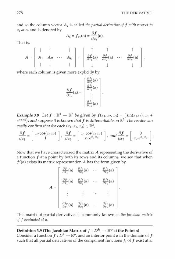
278 THE DERIVATIVE
and so the column vector Ai is called the partial derivative of f with respect toxi at a, and is denoted by
Ai = fxi (a) =*f
*xi(a).
That is,
A =
5
VV6
6 6 6
A1 A2 · · · Ak
7 7 7
7
WW8 =
5
VV6
6 6 6
-f
-x1(a) -f
-x2(a) · · ·
-f
-xk(a)
7 7 7
7
WW8 ,
where each column is given more explicitly by
*f
*xi(a) =
5
VVVVVV6
-f1-xi
(a)-f2-xi
(a)
...-fp-xi
(a)
7
WWWWWW8.
Example 3.8 Let f : R33 R2 be given by f (x1, x2, x3) =
,sin(x1x2), x1 +
ex2 x3-, and suppose it is known that f is differentiable on R3. The reader can
easily confirm that for each (x1, x2, x3) # R3,
*f
*x1=
9x2 cos(x1x2)
1
:,
*f
*x2=
9x1 cos(x1x2)
x3 ex2 x3
:, and
*f
*x3=
90
x2 ex2 x3
:.
"
Now that we have characterized the matrix A representing the derivative ofa function f at a point by both its rows and its columns, we see that whenf !(a) exists its matrix representation A has the form given by
A =
5
VVVVVVVVVVV6
-f1-x1
(a) -f1-x2
(a) · · ·-f1-xk
(a)
-f2-x1
(a) -f2-x2
(a) · · ·-f2-xk
(a)
......
. . ....
-fp-x1
(a) -fp-x2
(a) · · ·-fp-xk
(a)
7
WWWWWWWWWWW8
.
This matrix of partial derivatives is commonly known as the Jacobian matrixof f evaluated at a.
Definition 3.9 (The Jacobian Matrix of f : Dk $ Rp at the Point a)Consider a function f : Dk
3 Rp, and an interior point a in the domain of fsuch that all partial derivatives of the component functions fi of f exist at a.

THE DERIVATIVE FOR f : Dk , R
p 279
The Jacobian matrix of f at a is the p.k matrix denoted by J(a) and definedas
J(a) =
5
VVVVVVVVVVV6
-f1-x1
(a) -f1-x2
(a) · · ·-f1-xk
(a)
-f2-x1
(a) -f2-x2
(a) · · ·-f2-xk
(a)
......
. . ....
-fp-x1
(a) -fp-x2
(a) · · ·-fp-xk
(a)
7
WWWWWWWWWWW8
.
Notice that the above definition does not require the differentiability of f ata, but only that the individual partial derivatives exist at a. Just as for thegradient in the case f : Dk
3 R, the Jacobian matrix for any f : Dk3 Rp
can be constructed as long as all k first-order partial derivatives exist for eachcomponent function fi for i = 1, . . . , p. Just as with the gradient, the existenceof the Jacobian matrix for a mapping f at a point a is not enough to ensure theexistence of the derivative f ! there. What exactly is the relationship betweenthe Jacobian matrix and the derivative of a function f at a point a? What wehave seen so far is that if the function is already known to be differentiableat a, then the derivative at a is in fact the Jacobian matrix evaluated at a.From this we can conclude that if the Jacobian matrix J fails to exist at apoint a, the derivative of f will not exist there either. In other words, theexistence of J(a) is a necessary condition for the existence of f !(a). In general,this necessary condition is not a sufficient condition, however. That is, thereexist functions f : Dk
3 Rp for which the Jacobian J(a) exists at a, but thederivative f !(a) fails to exist. Fortunately, there is an extra condition which,when combined with the existence of the Jacobian matrix at a, guarantees theexistence of f ! there. When these two conditions are satisfied, we then willhave f !(a) = J(a). The moral of the story once again is: The differentiabilityof a function of more than one variable requires more than just the existence of thefirst-order partial derivatives.
Theorem 3.10 (Sufficient Conditions for Existence of f ! at the Point a)Let f : Dk
3 Rp have component functions fi : Dk3 R for i = 1, . . . , p,
and let a be an interior point of Dk . If the partial derivatives -fi-xj
for i = 1, . . . , p
and j = 1, . . . , k exist in a neighborhood of a and are continuous at a, then f isdifferentiable at a and f !(a) = J(a).
PROOF Consider the simpler case of f : D23 R first, and assume that fx
and fy satisfy the hypotheses of the theorem at and near the interior point a =(a, b) # D2. We will show that f !(a) = %f (a). To do this, we must establishthat for any given ! > 0 we can find . > 0 such that |x " a| < . implies

280 THE DERIVATIVE
|f (x) " f (a) " %f (a) (x" a)| + ! |x" a| .
This vector version of the !, . definition of differentiability is not quite asuseful in this particular instance, and so we translate it into its correspondingcomponentwise form as follows. We will show that, for x = (x, y) # D2,
whenever%
(x " a)2 + (y " b)2 < ., we have
&&f (x, y) " f (a, b) " (x " a)fx(a, b) " (y " b)fy(a, b)&&+ !
*(x " a)2 + (y " b)2.
To this end, we consider
f (x, y) " f (a, b) " (x " a) fx(a, b) " (y " b) fy(a, b)
= f (x, y) " f (a, y) " fx(a, y) (x" a) (6.28)
+f (a, y) " f (a, b) " fy(a, b) (y " b) + [fx(a, y) " fx(a, b)] (x" a).
Since fx(a, y) exists for y near b, there exists .1 > 0 such that
|x " a| < .1 ) |f (x, y) " f (a, y) " fx(a, y) (x" a)| + (3 |x " a|.
Similarly, since fy(a, b) exists, there exists .2 > 0 such that
|y " b| < .2 ) |f (a, y) " f (a, b) " fy(a, b) (y " b)| + (3 |y " b|.
Finally, since fx is continuous at (a, b), there exists .3 > 0 such that
|y " b| < .3 ) |fx(a, y) " fx(a, b)| < (3 .
Overall, letting . = min (.1, .2, .3), we have that%
(x " a)2 + (y " b)2 < .implies both |x " a| < . and |y " b| < ., which in turn imply that
|f (x, y) " f (a, b) " fx(a, b) (x" a) " fy(a, b) (y " b)|
+(3 |x " a| + (
3 |y " b| + (3 |x " a| (6.29)
+ !
*(x " a)2 + (y " b)2.
The first inequality in expression (6.29) is obtained by substituting (6.28) intothe absolute value bars on the left-hand side, followed by two applicationsof the triangle inequality. With this, the special case of the theorem is proved.The case for f : Dk
3 R with k > 2 is left as an exercise.
We consider now another case, namely, f : D23 R2. Suppose that for x =
(x, y) # D2, and f : D23 R2, the function f (x) is given by
f (x) = (g(x, y), h(x, y)) ,
where gx, gy, hx, and hy satisfy the hypotheses of the theorem at and nearthe point a = (a, b) # D2. We will show that f is differentiable at a with
f !(a) = J(a) =
5
6gx(a, b) gy(a, b)
hx(a, b) hy(a, b)
7
8 .
Since gx, gy, hx, and hy exist in a neighborhood of the point a = (a, b) and

THE DERIVATIVE FOR f : Dk , R
p 281
are continuous there, it follows from the case already proved that each ofthe component functions g and h are differentiable at the point a = (a, b).Therefore, for ! > 0 there exists . > 0 such that whenever |x"a| < . we have
&&g(x) " g(a) " g!(a) (x" a)&& + (
2 |x " a|,
and &&h(x) " h(a) " h! (a) (x" a)&&+
(2 |x " a|.
From this we obtain that whenever |x " a| < ., we have
|f (x) " f (a) " J(a) (x " a)|
=&&,g(x) " g(a) " g!(a) (x" a) , h(x) " h(a) " h!(a) (x" a)
-&&
+
&&g(x) " g(a) " g!(a) (x" a)&& +
&&h(x) " h(a) " h!(a) (x " a)&& (Why?)
+(2 |x " a| + (
2 |x" a|
= ! |x " a|.
This completes the proof for f : D23 R2. The more general case is handled
similarly and is left to the exercises. #
! 6.62 Prove the above theorem for the case f : D3 , R. Can you prove it for the
more general f : Dk , R?
! 6.63 Prove the above theorem for the case f : D3 , R
2. Can you prove it for the
more general f : Dk , R
p?
Theorem 3.10 is a very practical theorem. It allows one to avoid direct appli-cation of the derivative definition when trying to determine f ! for a functionf : Dk
3 Rp. More specifically, it says that if one constructs the Jacobianmatrix of first-order partial derivatives, and the partial derivatives all existin a neighborhood of a and are all continuous at a, then f ! exists at a and isgiven by J(a). That is, in many cases we can simply construct the Jacobianmatrix and then confirm that it is the derivative!
Example 3.11 Consider the function g : R 3 R2 given by
g(t) =,g1(t) , g2(t)
-=,t2 , et
-.
It is easy to see that g!(t) is given by
g!(t) =
9g&1(t)
g&2(t)
:=
92tet
:,
for all t. (Why?) "
Example 3.12 Consider the function f : D23 R2 given by
f (x, y) =
2exy
x,%
sin y
3
defined on the strip D2 = ("-, 0) . (0, %). If we denote the two component

282 THE DERIVATIVE
functions of f by f1 and f2 we have for all (x, y) # D2,
*f1
*x=
(xy " 1)exy
x2,
*f1
*y= exy,
and*f2
*x= 0,
*f2
*y=
cos y
2,
sin y,
all of which are continuous on D2. Therefore, f is differentiable on D2 andthe Jacobian matrix gives us the derivative as
f !(x, y) =
5
V6
(xy"1)exy
x2 exy
0 cos y2$
sin y
7
W8 .
"
Example 3.13 Consider the function given by
f (x, y) =
E xyx2+y2 (x, y) $= (0, 0)
0 (x, y) = (0, 0).
Clearly the first-order partial derivatives of f with respect to x and y exist atthe origin, since *f
*x(0, 0) = lim
x(0
f (x, 0) " f (0, 0)
x " 0= 0,
and *f
*y(0, 0) = lim
y(0
f (0, y) " f (0, 0)
y " 0= 0.
But this function can’t be differentiable at the origin, since
f (x, mx) =mx2
x2 + m2x2=
m
1 + m2
is enough to show that f isn’t even continuous there. It is left as an exerciseto show that *f/*x and *f/*y are not continuous at the origin. "
! 6.64 In the previous example, (f/(x and (f/(y can’t both be continuous at theorigin. Why? Show that both (f/(x and (f/(y are not continuous at the origin.
The following result is a generalization of Theorem 2.6 on page 262.
Proposition 3.14 Let Dk be a connected open subset of Rk, and suppose that f :Dk
3 Rp is differentiable on Dk with f !(x) = 0 for all x # Dk . Then there existsa constant vector c # Rp such that f (x) = c for all x # Dk .
! 6.65 Prove the above theorem.
! 6.66 Consider f : Dk , R
p. If there exists a constant vector c " Rp such that
f (x) = c for all x " Dk , show that f !(x) = 0 for all interior points x " D
k .

THE DERIVATIVE FOR f : Dk , R
p 283
3.2 Some Useful Results
In this subsection we develop the higher-dimensional analogues of some ofour earlier “useful results.“ Note that functions f : Dk
3 Rp have no “lo-cal extrema results,“ nor is there a version of Rolle’s theorem that applies tothem. This is because higher-dimensional Euclidean spaces lack the specialorder properties possessed by R.
Algebraic Results
The following result is analogous to Theorem 1.9 on page 244 and Proposi-tion 2.14 on page 270.
Proposition 3.15 (Algebraic Properties of the Derivative)Suppose the functions f : Dk
3 Rp and g : Dk3 Rp are differentiable at the
interior point a # Dk . Thena) f ± g is differentiable at a, and (f ± g)! (a) = f !(a) ± g!(a).
b) cf is differentiable at a, and (cf )! (a) = cf !(a) for c # R.
c) f · g is differentiable at a, and (f · g)! (a) = f (a)g!(a) + g(a)f !(a).
! 6.67 Prove the above theorem. Note that in part c) the terms f (a)g!(a) and g(a)f !(a)are products of a p-dimensional row vector with a p + k matrix. That is, (f · g)! (a) isa 1 + k matrix, as it should be. Why is the corresponding part d) of Theorem 1.9 andProposition 2.14 not represented here?
The higher-dimensional version of the chain rule for functions f : Dk3 Rp
is a generalization of the more familiar one corresponding to one dimen-sional Euclidean space, as it must be. We prove this important theorem next.
Theorem 3.16 (The Chain Rule for f : Dk $ Rp)Suppose f : Dk
3 Dp is differentiable at the interior point a # Dk, and g :Dp
3 Rm is differentiable at the interior point b = f (a) # Dp. Then the compositefunction h / g;f : Dk
3 Rm is differentiable at a # Dk and h!(a) = g!(b) f !(a).
Note that h!(a) = g!(b) f !(a) in the above theorem is a product of matrices. Inparticular, g!(b) is an m . p matrix and f !(a) is a p . k matrix.
PROOF 8 We begin the proof with a rather convenient choice of function. Wedefine the function G : Dp
3 Rm as follows:
G(y) /
Eg(y)"g(b)"g! (b)(y"b)
|y"b| for y $= b and y # Dp
0 for y = b.
8We follow [Fit95] for the proof.

284 THE DERIVATIVE
This function G is continuous at y = b (Why?). Rearranging the expressionfor G(y) gives
g(y) " g(b) = g!(b)(y " b) + G(y)|y " b| for all y # Dp.
Letting y = f (x) and substituting f (a) for b yields
h(x) " h(a) = g!(b)(f (x) " f (a)) + G (f (x)) |f (x) " f (a)|. (6.30)
Subtracting g!(b)f !(a)(x " a) from both sides of (6.30), and dividing bothsides by |x" a| under the assumption x $= a obtains the lengthy expression
h(x)"h(a)"g! (b)f ! (a)(x"a)|x"a| = g!(b)
0f(x)"f(a)"f !(a)(x"a)
|x"a|
1+ G (f (x)) |f(x)"f(a)|
|x"a| .
(6.31)Now, since f is differentiable at a, the following is true:
1. limx(a
0f(x)"f(a)"f !(a)(x"a)
|x"a|
1= 0.
2. There exists .1 > 0 and a constant C > 0 such that 0 < |x " a| < .1 )
|f(x)"f(a)||x"a| + C
,1 + |f !(a)|
-. (Why?)
Also, by continuity of f and G, we have that
3. limx(a G (f (x)) = G (f (a)) = G(b) = 0.
Considering the lengthy expression (6.31), along with these last three facts,yields
limx(a
h(x) " h(a) " g!(b) f !(a)(x " a)
|x" a|= 0.
That is,h!(a) = g!(b) f !(a). #
! 6.68 Show that the function G : Dp , R
m in the above proof is continuous aty = b. Also, answer the (Why?) question following remark number 2.
Note again that the derivative h!(a) is the product of matrices g!(b) and f !(a).This is found to be either strange or convenient, depending on one’s mathe-matical experience.
Mean Value Theorems and Taylor’s Theorems with Remainder
Recall that we postponed stating and proving the mean value theorem andTaylor’s theorem with remainder for functions f : Dk
3 R in the previoussection. This was because we needed the chain rule in the f : Dk
3 Rp
case. Now that this chain rule is established, we can tie up these loose ends.Before stating and proving these results, we take the time to clarify whatis meant by the phrase “between two points“ in higher-dimensional spaces.One natural interpretation of this phrase is “on the line segment joining“the two points. In the discussion that follows, we denote the line segmentjoining two points p1 and p2 in Rk by [p1, p2] or (p1, p2). Square brackets

THE DERIVATIVE FOR f : Dk , R
p 285
will be used to indicate that the segment includes the endpoints p1 and p2,while parentheses will be used to indicate that the segment does not includethe endpoints p1 and p2. For example, the line segment joining p1 and p2
but not containing either is the set (p1, p2) /
.p # Rk : p = p1 + t (p2 "
p1), for 0 < t < 1/
.
Theorem 3.17 (The Mean Value Theorem for f : Dk $ R)Let Dk be an open subset of Rk and suppose that f : Dk
3 R is differentiable onDk. Suppose p1 and p2 are two distinct interior points in Dk such that the segment(p1, p2) is entirely contained within Dk. Then, there exists a point q on the segment(p1, p2) such that
f (p2) " f (p1) = f !(q) (p2 " p1).
PROOF 9 To prove the result, we define a real-valued function of a single realvariable, g(t) / f (p1 + t (p2 " p1)) . It is easy to see that g is continuous on[0, 1] and differentiable on (0, 1), with derivative
g&(t) = f ! (p1 + t (p2 " p1)) (p2 " p1).
Then there exists / # (0, 1) such that g(1)" g(0) = g&(/ ). (Why?) Defining q byq / p1 + / (p2 " p1), we obtain
f (p2) " f (p1) = f !(q) (p2 " p1),
and the theorem is proved. #
! 6.69 Can you use this version of the mean value theorem to prove the version ofRolle’s theorem given by Proposition 2.18 on page 272?
To round out our list of “useful results“ for functions f : Dk3 R, we now
develop a version of Taylor’s theorem with remainder for real-valued func-tions of several variables. For convenience, we will handle the f : D2
3 R
case and leave the more general f : Dk3 R case to the reader. For conve-
nience, assume f : D23 R has as many mixed partial derivatives as needed.
Fix interior point a # D2 and x # D2 near a. As in the proof of the meanvalue theorem, we define
g(t) / f (a + t (x " a)) , (6.32)
where a = (a, b), and x = (x, y). Applying the one-dimensional version ofTaylor’s theorem with remainder to g, centered at t = 0, gives
g(t) =n+
j=0
g(j)(0)
j!tj + Rn(t).
Setting t = 1 obtains
9We follow [Ful78].

286 THE DERIVATIVE
g(1) =n+
j=0
g(j)(0)
j!+ Rn(1), (6.33)
where, for some ) # (0, 1), Rn(1) is given by
Rn(1) =g(n+1)())
(n + 1)!. (6.34)
But (6.32) yields that g(1) = f (x), and so (6.33) becomes
f (x) =n+
j=0
g(j)(0)
j!+
g(n+1)())
(n + 1)!,
where we have used (6.34) to replace Rn(1). We denote the finite sum on theright-hand side of the above formula for f (x) by Pn(x), that is, we define
Pn(x) /
;nj=0
g(j)(0)j! . Though a bit difficult to see, Pn(x) is actually the nth-
degree Taylor polynomial for f (x) centered at a. To see this more clearly, weuse (6.32) to compute the first few terms in the sum:
g(0) = f (a)
g&(0) = (x " a)fx(a) + (y " b)fy(a)
g&&(0) = (x " a)2fxx(a) + (x " a)(y " b)fxy(a)
+ (x " a)(y " b)fyx(a) + (y " b)2fyy(a).
Notice that g&(0) is a first-degree polynomial in x and y, and g&&(0) is a second-degree polynomial in x and y, where x and y are the components of the vectorx. Of course, just as in the one-dimensional case, we can approximate f (x) byits Taylor polynomial Pn(x).10
! 6.70 Compute g###(0). Can you find a pattern for g
(j)(0)?
! 6.71 Find P2(x) for the function f (x) = sin x sin y.
In order to state Taylor’s theorem with remainder in a more compact form,we take the time now to develop a bit of informal operator notation. It willgreatly simplify the form of the derivative terms g(j)(0), which can otherwiseseem rather complicated. We do this in the f : D2
3 R case for convenience,although it is readily generalizable to the f : Dk
3 R case. Define the differ-ential operator L by11
10Just as in the one-dimensional case, if Pn(x) exists for all n within a neighborhood of a,and if Rn(x) ( 0 as n ( ' within that neighborhood, we refer to the resulting associated“infinite degree Taylor polynomial“ as the Taylor series of f centered at a. Again, Taylor series willbe discussed more fully in Chapter 9.
11Note that the differential operator could have been more explicitly denoted by La, in thatthe point a = (a, b) # R2 is specific to L. However, to retain a less cluttered notation we willdispense with the subscript and work under the assumption that the context will make it clearabout which point we are expanding our Taylor polynomial.

THE DERIVATIVE FOR f : Dk , R
p 287
L / (x " a)*
*x+ (y " b)
*
*y.
Applying this operator to the function f , we have
Lf = (x " a)*f
*x+ (y " b)
*f
*y.
We also define “powers“ of L in the following formal, nonrigorous manner,12
namely,
L2 /
((x " a) -
-x + (y " b) --y
)2
/
((x " a) -
-x + (y " b) --y
)((x " a) -
-x + (y " b) --y
)
= (x " a)2 -2
-x2 + (x " a)(y " b) -2
-x-y + (x " a)(y " b) -2
-y-x + (y " b)2 -2
-y2 .
Likewise, we define Lj for any j # N according to
Lj /
((x " a) -
-x + (y " b) --y
)j.
It is not hard to show that
g(j)(0) =,Ljf
-(a), (6.35)
and so
f (x) =n+
j=0
,Ljf
-(a)
j!+ Rn(x), (6.36)
where Rn(x) is given by
Rn(x) =
,L(n+1)f
-(!)
(n + 1)!for some ! # (a, x). (6.37)
! 6.72 Verify (6.35) and therefore that equations (6.36) and (6.37) can be obtainedfrom the one-dimensional Taylor’s theorem with remainder, Theorem 1.22 on page 252,applied to the function g.
We now formally state the theorem implied by our special-case derivation.
Theorem 3.18 (Taylor’s Theorem with Remainder for f : Dk $ R)Suppose all partial derivatives of order n of the function f : Dk
3 R are continuouson Dk, and suppose all partial derivatives of order n + 1 exist on Dk . Fix interiorpoint a # Dk and fix r > 0 such that Nr(a) ' Dk. Define the differential operatorL by
L /
k+
i=1
(xi " ai)-
-xi.
Then for x # Nr(a),f (x) = Pn(x) + Rn(x),
12We use a subscript rather than an exponent to remind the reader that the resulting operatoris not actually the associated operator power of L. To see this, simply consider the case of Lapplied to Lf , i.e., L(Lf ). The result is not given by what we refer to as L2f .

288 THE DERIVATIVE
where
Pn(x) =n+
j=0
,Ljf
-(a)
j!and Rn(x) =
,L(n+1)f
-(!)
(n + 1)!
for some ! # (a, x).
! 6.73 How does the expression for L2f simplify for a function f : D2 , R that
satisfies fxy = fyx?
! 6.74 Write the derivation of Taylor’s theorem with remainder for f : Dk , R.
! 6.75 Can you derive the associated mean value theorem from Taylor’s theoremwith remainder for f : D
2 , R? How about for f : Dk , R?
Now that we have established the mean value theorem and Taylor’s theoremfor functions f : Dk
3 R, results that were left unfinished in the previoussection, we can refocus our attention on the functions specific to this section,namely, f : Dk
3 Rp. There are versions of the mean value theorem andTaylor’s theorem with remainder in this more general case as well, althoughthey are a bit different from the previous cases we have seen.
Theorem 3.19 (The Mean Value Theorem for f : Dk $ Rp)Let Dk be an open subset of Rk , and suppose that f : Dk
3 Rp is differentiable onDk . Suppose p1 and p2 are two distinct interior points in Dk such that the segment(p1, p2) is entirely contained within Dk . Then, there exist points q1, q2, . . . , qp
on the segment (p1, p2) such that
f (p2) " f (p1) =
5
VVVVV6
8 f !
1(q1) 3
8 f !
2(q2) 3
...
8 f !p(qp) 3
7
WWWWW8(p2 " p1).
! 6.76 Prove the above theorem along the lines of Theorem 3.17 on page 285. In whatsignificant way does it differ from previous versions of the mean value theorem?
! 6.77 Let f : R2 , R
2 be given by f (x, y) =(x
2 + 4y, x3 & y2)
. If a = (0, 0), and
b = (1, 0), show that there does not exist a point ! " R2 such that f (b) & f (a) =
f !(!) (b & a).
Corresponding to the above mean value theorem for functions f : Dk3 Rp
is the following Taylor’s theorem with remainder.

THE DERIVATIVE FOR f : Dk , R
p 289
Theorem 3.20 (Taylor’s Theorem with Remainder for f : Dk $ Rp)Consider the function f : Dk
3 Rp given by f (x) =,f1(x), f2(x), . . . , fp(x)
-
for all x # Dk , where each fi is a real-valued function on Dk . Suppose all partialderivatives of order n of the functions fi are continuous on Dk for i = 1, 2, . . . p,and suppose all partial derivatives of order n + 1 of the functions fi exist on Dk fori = 1, 2, . . . p. Fix a # Dk and r > 0 such that Nr(a) ' Dk . Then, for x # Nr(a),
f (x) = Pn(x) + Rn(x)
where
Pn(x) =
I
Jn+
j=0
,Ljf1
-(a)
j!, . . . ,
n+
j=0
,Ljfp
-(a)
j!
K
L ,
and
Rn(x) =
C,L(n+1)f1
-(!1)
(n + 1)!, . . . ,
,L(n+1)fp
-(!p)
(n + 1)!
D
for some !1, !2, . . . , !p # (a, x).
! 6.78 Prove the above theorem.
! 6.79 Consider the function f : R2 , R
2 given by f (x, y) =,exy, x sin y
-. Find
P3(x) and R3(x) centered at 0.
3.3 Differentiability Classes
Functions can be conveniently categorized according to how many contin-uous derivatives they possess, i.e., how many derivatives they possess thatare themselves continuous functions. For example, one such class of func-tions of interest in analysis is the class of functions having a continuous firstderivative. Such functions are often referred to as continuously differentiablefunctions. The following definition generalizes this classification idea.
Definition 3.21 A function f : D13 R is called a Cn function on D1, or is
considered to be in the class Cn(D1), if f has n derivatives that are themselvescontinuous functions on D1.
If f has continuous derivatives of all orders on D1 we say that f is a C"
function on D1 and consider it to be in the class C'(D1).
Example 3.22 Consider f : D13 R given by f (x) = x7/2, where D1 =
("1, 1). Then f # C3(D1). (Why?) "
! 6.80 Verify the claim made in the above example.

290 THE DERIVATIVE
Note that a function f : D13 R that is Cn(D1) is also Cm(D1) for m < n.
In fact, the differentiability classes have a nested relationship. Often, the do-main of interest in using the above terminology is clear from the context ofthe problem, in which case D1 won’t be specified explicitly and the functionwill simply be referred to as a Cn function. For example, if f is C3 ((0, 1)), andthe interval (0, 1) is unambiguously understood to be the domain of interest,we will simply say that f is C3. It is worth pointing out that identifying f asC3 does not preclude the possibility that f might in fact be C4 or even Cn forsome other n > 3. While one usually categorizes a function into its appropri-ate Cn class according to the largest n for which the function qualifies, it isnot necessary, and in certain instances not very convenient to do so. Also, iff is Cn, but is not Cn+1, this does not imply that f does not have a derivativeof order (n + 1), but only that such a derivative (if it exists) is not continuous.It is worth mentioning that, in general, the higher the differentiability classto which it belongs, the “better behaved“ a function can be expected to be. Aclue as to why this is so is the fact, proved in Chapter 5, that if a function iscontinuous at a point then the function remains bounded in some neighbor-hood of that point. Therefore, if a function f is C1, for example, its derivativef & remains bounded in some neighborhood of each point of its domain. If thefunction is differentiable but not C1, then its derivative may be unboundedat any point in its domain where f & is not continuous. This possibility canlead to the function f having unusual behavior at or near such a point.
Just as we categorized a function f : D13 R having n continuous deriva-
tives on D1 as being Cn(D1), we can likewise categorize functions f : Dk3
R as Cn(Dk) according to how many continuous partial derivatives they have.
Definition 3.23 A function f : Dk3 R is called a Cn function on Dk , or
is considered to be in the class Cn(Dk), if all partial derivatives (includingmixed) of order n exist and are continuous on Dk . We say that f is a C"
function on Dk if it has continuous partial derivatives of all orders on Dk . Inthis latter case, we consider f to be in the class C'(Dk).
Example 3.24 Let f (x, y) = x(x2 + y2)3/2 on all of R2. Then it is not hard toverify that fx(x, y) = 3x2(x2 + y2)1/2 + (x2 + y2)3/2, and fy(x, y) = 3xy(x2 +
y2)1/2. From this we determine that f is at least C1(R2). In determining thesecond-order partial derivatives, one can show that fxy does not exist at (0, 0).Therefore, f cannot be in C2(R2). "
! 6.81 In the above example, verify that fxy does not exist at (0, 0). Also, find theother second-order partial derivatives of f , and verify that the origin is the only dis-continuity among them.
! 6.82 For the same function as in the last example, suppose we restrict the domainto D
2 . {(x, y) : xy %= 0}. The result is a new function (since the domain is dif-

THE DERIVATIVE FOR f : D , C 291
ferent from the function in the example); call it g. What is the largest n for whichg " C
n(D2)?
! 6.83 Can you extend Definition 3.23 in a natural way to be able to similarly cate-gorize functions f : D
k , Rp?
The concepts of derivative and differentiability play an even more significantrole for functions of a complex variable than for functions of real variables.In fact, we will ultimately discover that if a complex function f : D 3 C isdifferentiable on D ' C, then f must be C' on D. This is a significant re-sult. It means that differentiable complex functions can’t exhibit the unusualbehaviors that some differentiable real functions might exhibit. We begin dis-cussing this very important case next.
4 THE DERIVATIVE FOR f : D 3 C
In this section we investigate the concept of differentiation for complex val-ued functions of a complex variable, commonly referred to as complex func-tions. There are in fact two ways to view such functions. From a geometricpoint of view, since the complex variable z can be thought of as a vector hav-ing components x and y, a function f : D 3 C can be thought of as a specialcase of f : D2
3 R2. That is, a complex function is a function from the(complex) plane to itself. From an algebraic point of view, since C is a field, acomplex function can be thought of as a function that takes an element of thefield C to another element of the field C. That is, just like real-valued func-tions of a single real variable, a complex function is a function from a fieldto itself. The notation we adopt for complex functions follows from this al-gebraic perspective. Since we are discussing complex-valued functions of asingle complex variable, it is common practice to use the same style font asfor a real-valued function of a single real variable, namely f (z) (rather thanf (z)). Although the algebraic view “wins out“ notationally, we will see thatcomplex functions can be more rewardingly viewed from the geometric per-spective. (See, for example, the discussion of complex functions as mappingsin Chapter 10.) In the end, we hope to reconcile both points of view as theypertain to the world of complex functions. As already mentioned in Chapter4, we note that in the context of complex functions f : D 3 C, the domainwill be denoted by D rather than D2 to distinguish this rather special classof functions from the real case(s). Finally, before we begin our discussion ofderivatives of complex functions, we must clarify our position on the termi-nology common to the theory of functions of a complex variable. In mosttexts on complex function theory, a complex function that is differentiable onan open set D ' C is referred to as analytic (or, somewhat less commonlynowadays, holomorphic) on D. In some such texts, a complex function is evendefined to be analytic on such a set D exactly when it is differentiable there.It is in fact true that such differentiable complex functions are analytic, but inour development of the subject we will not define analyticity until later in the

292 THE DERIVATIVE
text.13 Once we have defined the term analytic, we will show that a complexfunction that is differentiable on an open set D must be analytic there. Thereader may then return to this section and replace each instance of the phrase“complex function differentiable on the open set D ' C“ with “analytic com-plex function on the open set D ' C,“ thereby gaining consistency betweenthe statements of theorems in this work and the corresponding statementsin other, more traditional treatments. It should be noted, however, that realfunctions that are differentiable on an open set are not necessarily analyticthere, no matter what text you are reading. This is one of the significant waysin which complex functions and real functions differ from each other.
4.1 Three Derivative Definitions Again
Let us look more carefully now at the algebraic representation of the deriva-tive. Just as in the real case, we will present an “official“ derivative definition,as well as two equivalent, alternative versions that will prove to be quitepractical in our work. As in the real case, our “official“ version is the linearapproximation version.
The Linear Approximation Version
Definition 4.1 (Derivative of f : D $ C at the point z0) For a complex func-tion f : D 3 C and z0 # Int(D), we say that f is differentiable at z0 if thereexists a complex number A such that the linear function p : D 3 C given by
p(z) = f (z0) + A (z " z0) satisfies limz(z0
f (z) " p(z)
|z " z0|= 0.
In this case, we refer to the complex number A as the derivative of f at z0,
and denote it thereafter by f &(z0) or dfdz (z0).
Note that the absolute value bars in the denominator of the above limit ex-pression are not really necessary, just as in the case of a real-valued functionf : D1
3 R. This is because the numerator f (z) " p(z) and the denominatorz " z0 are members of the same field, and so their ratio (without absolutevalue bars) is well defined as long as the denominator is nonzero. We haveretained the absolute value bars only to be consistent with the correspondingreal function versions of the definition.
The Difference Quotient Version
Omitting the absolute value bars mentioned above, and a bit of rearrange-ment, leads us naturally to the convenient, practical, and equivalent differ-ence quotient version of the derivative of a complex function.
13Our definition of analyticity, in fact, will rely on the existence of a convergent Taylor seriesfor the function in question. This will provide us with a definition of analyticity that extendsconsistently to real functions.

THE DERIVATIVE FOR f : D , C 293
A complex function f : D 3 C is differentiable at z0 # Int(D) if and only if
limz(z0
f (z) " f (z0)
z " z0
exists. In this case, we denote the limit by f &(z0) or dfdz (z0).
We emphasize again that this version of the derivative definition is onlyavailable in this case and that of a real-valued function of a single real vari-able. In each of these cases, the function is a mapping from a field to itself,and so the difference quotient (without absolute value bars) is well defined.
The $, % Version
Likewise, the !, . version of the definition of the derivative is often conve-nient to apply.
The function f : D 3 C is differentiable at z0 # Int(D) and has derivative f &(z0)there if and only if for each ! > 0 there exists . > 0 such that
|z " z0| < . ) |f (z) " f (z0) " f &(z0) (z " z0)| + ! |z " z0|.
The equivalence of these three definitions is stated in the following result,an analog to Theorem 1.2 on page 238.
Proposition 4.2 Consider f : D 3 C and z0 # Int(D). The following threestatements are mathematically equivalent.
a) limz(z0f (z)"f (z0)
z"z0= A.
b) There exists A # C such that for any ! > 0 there exists . > 0 such that
|z " z0| < . ) |f (z) " f (z0) " A (z " z0)| + ! |z " z0|.
c) There exists A # C such that the function p : D 3 C given by
p(z) = f (z0) + A (z " z0) satisfies limz(z0
f (z) " p(z)
|z " z0|= 0.
When any one (and therefore all three) of these statements is true, the function f isdifferentiable at z0 # Int(D) with derivative f &(z0) = A.
! 6.84 Prove the above result.
! 6.85 For each f (z) below, use the difference quotient formulation to verify that thegiven f
#(z0) is as claimed. Then use the $, . version to prove that the derivative is the

294 THE DERIVATIVE
given f#(z0).
a) f (z) = c for D = C, constant c " C, f#(z0) = 0 for all z0 " D
b) f (z) = z3 for D = C, f
#(z0) = 3z20 for all z0 " D
c) f (z) = z!1 for D = C \ {0}, f
#(z0) = &z!20 for all z0 " D
d) f (z) = zn for D = C, n " Z
+, f#(z0) = nz
n!10 for all z0 " D
e) f (z) = zn for D = C \ {0}, n " Z
!, f#(z0) = nz
n!10 for all z0 " D
f ) f (z) = sin z for D = C, f#(z0) = cos z0, for all z0 " D
g) f (z) = cos z for D = C, f#(z0) = & sin z0, for all z0 " D
A hint for part f) is to consider the trigonometric identity
sin % & sin & = 2 cos(
%+'
2
)sin
(%!'
2
).
Just as for real functions, when the derivative of a complex function f at apoint z0 exists, it is unique. This fact is given in the following proposition,the proof of which is left to the reader.
Proposition 4.3 Consider f : D 3 C and z0 # Int(D). If f &(z0) exists, then it isunique.
! 6.86 Prove the above result.
It is also true for complex functions that differentiability implies continuity.We state this too as a separate result, mirroring Proposition 1.7 on page 242in the real case almost exactly. Once again, the proof is left to the reader.
Proposition 4.4 Let the function f : D 3 C be differentiable at z0 # Int(D).Then f is continuous at z0 as well.
! 6.87 Prove the above result.
Higher-Order Derivatives
Of course, just as for real functions, a function f : D 3 C might be differen-tiable at more than just a single point of its domain. In fact, we may considerall the points Df ! ' D at which f is differentiable as the domain of the func-tion f & : Df ! 3 C. That is, the derivative of f is itself a complex function, andwe say that f is differentiable on Df ! . If z0 is an interior point of Df ! , we mayconsider whether f & has a derivative at z0. We can determine this by checkingwhether the limit
limz(z0
f &(z) " f &(z0)
z " z0= B

THE DERIVATIVE FOR f : D , C 295
for some complex number B. If so, then B = f &&(z0) is called the second deriva-tive of f at z0. In similar fashion, one may consider whether the third deriva-tive f &&&(z0) exists at z0, and more generally, whether the nth derivative f (n)(z0)exists at z0. Just as we found for real-valued functions of a single real variable,this derivative-generating scheme shows that it is necessary for the (n " 1)st
derivative to exist before one can consider the existence of the nth derivative.It is also necessary for the point z0 to be an interior point of the domain off (n"1) to consider the existence of f (n)(z0). Once again, this last fact impliesthat the domain of the nth derivative will be contained in the domain of the(n " 1)st.
4.2 Some Useful Results
Just as in the real function case, we list a few of the more convenient resultsthat allow for easier manipulation of derivatives for functions f : D 3 C. Webegin with the algebraic properties.
Algebraic Results
Proposition 4.5 (Algebraic Properties of the Derivative)Suppose the functions f : D 3 C and g : D 3 C are differentiable at z0 # Int(D).Then
a) f ± g is differentiable at z0, and (f ± g)& (z0) = f &(z0) ± g&(z0).
b) fg is differentiable at z0, and (fg)& (z0) = g(z0)f &(z0) + f (z0)g&(z0).
c) cf is differentiable at z0, and (cf )& (z0) = cf &(z0) for c # C.
d) (f/g) is differentiable at z0 provided g(z0) $= 0. In this case,
(f/g)& (z0) =g(z0)f &(z0) " f (z0)g&(z0)
(g(z0))2.
! 6.88 Prove the above result.
! 6.89 Consider f : D , C. If f# . 0 on D, what can you conclude about f? Does it
matter what kind of set D is?
! 6.90 Prove that the following functions f : C , C are differentiable on C.a) f (z) = z b) f (z) = z
n for n " Z+
c) f (z) = c0 + c1 z + c2 z2 + · · · + cn z
n for cj " C and n " N with cn %= 0.
! 6.91 Suppose p : C , C is given by p(z) = a0 + a1 z + a2 z2 + · · · + an z
n forn " N, aj " C for all 0 # j # n, and an %= 0, and q : C , C is given by q(z) =
b0 + b1 z + b2 z2 + · · · + bm z
m for m " N, bj " C for all 0 # j # m, and bm %= 0. Then,
for f : D , C given by f (z) = p(z)q(z) , where D = {z " C : q(z) %= 0}, show that f is
differentiable on D.

296 THE DERIVATIVE
Proposition 4.6 (The Chain Rule for f : D $ C)Suppose f : Df 3 C is differentiable at z0 # Int(Df ), and let Rf / f (Df ).Suppose Rf ' Dg . If g : Dg 3 C is differentiable at w0 = f (z0) # Int(Dg), thenh / g ; f : Df 3 C is differentiable at z0 # Int(Df ), and
h&(z0) = g&(w0)f &(z0) = g& (f (z0)) f &(z0).
! 6.92 Prove the chain rule for complex functions.
Lack of Local Extrema Results
Just as in the real case f : Dk3 Rp, there are no local extrema results for
functions f : D 3 C, nor is there a comparable version of Rolle’s theorem.After all, C is geometrically similar to R2, and both lack the special orderproperties possessed by R that are required. Also lacking in the complexfunction case is a version of the mean value theorem that would in some waydepend on Rolle’s theorem (recall that in the case f : D1
3 R one could showthat Rolle’s theorem implied the mean value theorem and vice versa). In fact,the reader is encouraged to work the following exercise, which provides acounterexample to this type of mean value theorem for complex functions.Later we will see that a different kind of mean value theorem holds in thiscase.
! 6.93 Let f : C , C be given by f (z) = z3, and consider the points z1 = 1 and z2 = i
as p1 and p2 in the statement of Theorem 3.17 on page 285. Show that there does notexist a complex number playing the role of q as described in that theorem.
As a consequence of the above discussion, there is no version of Taylor’stheorem with remainder that would have followed directly from the meanvalue theorem as was possible for f : D1
3 R and for f : Dk3 R. This
is not to say that there is no Taylor’s theorem with remainder for complexfunctions—there is! However, we will see in a later chapter that it is in aform that differs from the versions we have seen thus far. In particular, itsremainder is expressible in a way that does not involve a derivative of thefunction in question.
There is one very significant derivative result that is special to the class ofcomplex functions f : D 3 C. In fact, this result is named after not one, buttwo mathematicians worthy of note. Just as the Jacobian provided a conve-nient way to determine whether a real function f : Dk
3 Rp was differen-tiable at a point, the Cauchy-Riemann equations provide a means for doing thesame thing in the complex function case. We investigate this important set ofequations next.

THE DERIVATIVE FOR f : D , C 297
4.3 The Cauchy-Riemann Equations
The Cauchy-Riemann equations of complex function theory are arguablyamong the most significant results in analysis, providing a convenient char-acterization of differentiability for complex functions. We begin with an in-formal motivation, followed by a more careful, mathematically rigorous de-velopment.
An Informal Motivation for the Cauchy-Riemann Equations
For the moment, consider f (z) = u(x, y) + i v(x, y) from the geometric point ofview. At any point z = x+ i y in the domain of f , we have, with a slight abuseof notation,
f (z) = u(x, y) + i v(x, y) =,u(x, y), v(x, y)
-= f (x, y).
Here, u and v can be thought of as the real-valued component functions of avector-valued function f : D2
3 R2. The function f maps elements of D2 toR2, and so it clearly lends itself to the derivative definition from the previoussubsection. That is, if the derivative f &(z0) exists, it should take the form of a2 . 2 matrix A = f !(x0, y0), which must be the Jacobian matrix,14
J(x0, y0) =
5
VV6
ux(x0, y0) uy(x0, y0)
vx(x0, y0) vy(x0, y0)
7
WW8 .
There is more here, however, than meets the eye. We will see that for a com-plex function f : D 3 C to be differentiable implies much more than for avector valued function f : D2
3 R2. Since a significant difference betweenthe two situations is that C is a field, whereas R2 is not, the field propertymust be what gives complex functions their additional structure.
While the above 2. 2 matrix description of the derivative of f (z) at z0 seemsreasonable enough, now consider the function f (z) the way one considers areal-valued function of a single real variable, i.e., algebraically. The readercan readily verify that, consistent with (6.1) on page 235, the derivative off at z0 # C might also be viewed as the limit of the appropriate differencequotient,
limz(z0
f (z) " f (z0)
z " z0.
This limit, when it exists, must be a member of the field of which the differ-ence quotient is a member, i.e., the limit, when it exists, is a complex number.But just as with the geometric point of view, there is something of substanceyet hidden from us. In the comparison of complex functions f : D 3 C to
14Note that J(x, y) is a function of x and y, and not z, since each of its entries is a functionof x and y, and not z. When the context is clear, we will sometimes suppress the explicit xand y dependence in the entries of the Jacobian matrix to avoid a cluttered appearance in ourequations.

298 THE DERIVATIVE
real-valued functions f : D13 R, the only difference is that of dimension.
Since C is two-dimensional, the theory of complex functions is a richer the-ory than that of real-valued functions, as we will see.
How do we reconcile these seemingly different representations for the deriva-tive f &(z0) when it exists? We will “follow our noses“ and argue rather infor-mally first, then we will more rigorously justify what we have found in ourintuitive investigations. In the geometric point of view, the derivative is a2 . 2 matrix. In the algebraic point of view, the derivative is a complex num-ber. As we’ve seen in Chapter 2, there is a subset of 2 . 2 matrices that isnaturally isomorphic to the complex numbers, indicated by
a + ib 4
9a "bb a
:.
Comparing this to our 2 . 2 Jacobian matrix J(x0, y0), and viewing J(x0, y0)as a complex number via the above-mentioned isomorphism, yields
J(x0, y0) =
5
VV6
ux(x0, y0) uy(x0, y0)
vx(x0, y0) vy(x0, y0)
7
WW8 =
9a "bb a
:,
giving us a pair of equations that seemingly must hold true in order to makesense of our notion of derivative for complex functions. That is,
ux(x0, y0) = vy(x0, y0), and uy(x0, y0) = "vx(x0, y0).
In fact, these equalities relating the first-order partial derivatives of u and vat (x0, y0) are the Cauchy-Riemann equations that lie at the heart of complexfunction theory. Applying them to our Jacobian representation for f &(z0), andrecognizing the complex number represented by the resulting 2 . 2 matrixyields the correspondence
f !(x0, y0) =
5
VV6
ux(x0, y0) uy(x0, y0)
vx(x0, y0) vy(x0, y0)
7
WW883f &(z0) = ux(x0, y0) + i vx(x0, y0).
That is, the matrix representation of the derivative at z0 = x0 + i y0 is equiv-alent to the complex number having real part ux(x0, y0), and imaginary partvx(x0, y0). So, just as for a differentiable real function f : D1
3 R, a differen-tiable complex function can be seen to have as its derivative a member of thefield it maps from and into, even when starting from the geometric point ofview. This is not true for a general real function f : D2
3 R2 whose deriva-tive, if it exists, is not a member of R2, which itself is not a field. Also, whilewe can represent the derivative of a differentiable complex function in matrixform, the set of possible candidates is restricted to a very special class of 2.2

THE DERIVATIVE FOR f : D , C 299
matrices, namely, a subset of matrices isomorphic to the complex numbers.15
This last remark deserves further comment, since it is directly related to oneof the key ways in which complex functions differ from their real counter-parts. Recall that Theorem 3.10 from the last section gave us the followingresult. For a real function f : D2
3 R2 given by f (x, y) = (f1(x, y), f2(x, y)),
if each partial derivative, -f1-x , -f1
-y , -f2-x , and -f2
-y exists in a neighborhood of
the point (x0, y0) # D2 and is continuous at (x0, y0), then the function f isdifferentiable at (x0, y0) and f !(x0, y0) is given by J(x0, y0). Although a com-plex function f (z) = u(x, y) + i v(x, y) can also be viewed in certain ways as amapping from a subset of the plane to itself, the similarity runs only so deep.In fact, for such a complex function Theorem 3.10 is not enough to guaran-tee differentiability at a point z0. As already described, the Cauchy-Riemannequations impose an extra set of conditions that must be satisfied by a com-plex function in order for the derivative f &(z0) to exist, an extra set of condi-tions that effectively restrict the set of 2 . 2 Jacobian matrices available for acomplex function to qualify as differentiable at a point z0.
Example 4.7 Suppose f : C 3 C is given by f (z) = z + z = 2x. Viewing f
as f : D23 R2, we have f (x, y) = (2x, 0), and J(x, y) =
92 00 0
:. From this
we see that the Jacobian matrix exists, and each entry is in fact a continuousfunction on all of R2. Therefore f is differentiable as a function from R2 toR2. Furthermore, in this case the Jacobian matrix is the derivative. However,
the Jacobian matrix is not of the form
9a "bb a
:, and so we infer that f is
not differentiable as a function from C to C. "
Example 4.8 Suppose f : C 3 C is given by
f (z) = z2 =(x2
" y2)
+ i 2xy.
Then u(x, y) = x2" y2 and v(x, y) = 2xy. If we view f as f : R2
3 R2, thenf (x, y) =
,x2
" y2, 2xy-, and the Jacobian is given by
J(x, y) =
92x "2y2y 2x
:.
It is clear that all of the entries of J(x, y) are continuous for all values of x andy, and so the derivative f ! exists and is J(x, y) at all points of R2. Since the
Jacobian matrix has the form J(x, y) =
9a "bb a
:, we can identify f ! with
15The practical significance of the matrix representation for f !(z0) lies in its interpretation asa linear transformation. When applied to an element of the complex plane, the matrix has theeffect of scaling and rotating as discussed in subsection 3.6 of Chapter 1. The derivative of acomplex function at a point z0, when it exists, must be a scaling and a rotation at the point z0in this sense. We will consider this idea more carefully when we discuss conformal mappings inChapter 10.

300 THE DERIVATIVE
the complex number a + i b, or 2x + i 2y = 2z in this case. That is, according tothe matrix 4 complex number isomorphism,
f !(x, y) = J(x, y) =
92x "2y2y 2x
:83 f &(z) = 2x + i 2y = 2 z,
and so we can infer that when considered as a function from C to C, f & existsand will be given by f &(z) = 2 z. Note that this yields a derivative formula forthe complex function f (z) = z2 that is analogous to that of the real functionf (x) = x2. "
! 6.94 Using the same line of reasoning as in the last example, and recalling the factthat e
z = ex cos y + i e
x sin y, show that d
dzez can be inferred to be e
z .
! 6.95 Assuming that d
dzez = e
z , show that d
dzsin z can be inferred to be cos z, and
that d
dzcos z can be inferred to be & sin z. (Hint: Use the exponential forms of sin z
and cos z.)
! 6.96 Consider f : C , C given by f (z) = u(x, y) + i v(x, y) where u(x, y) = x2 + y
and v(x, y) = x2+y
2. Infer that the only z " C at which f#(z) might exist is z = & 1
2 &i12 .
! 6.97 Consider f : C , C given by
f (z) =(
5x + 12 x
2 + xy & y2)
+ i
(5y + 2xy + 1
2 y2 & 1
2 x2)
.
Use the method of this section to infer where f might be differentiable.
Rigorous Derivation of the Cauchy-Riemann Equations
Suppose f : D 3 C is differentiable at z0 = x0 + i y0 # Int(D) with deriva-tive f &(z0) = A1 + iA2, where A1, A2 # R. What are the values of A1 and A2?To determine this we will force z to approach z0 in the complex plane firsthorizontally and then vertically. To this end, substitute z = x + i y0 into Def-inition 4.1 given on page 292, and note that y0 is fixed. The definition thenyields that for any ! > 0 there exists . > 0 such that|x " x0| < . )
&&,u(x, y0)"u(x0, y0)"A1(x"x0)-+i
,v(x, y0)"v(x0, y0)"A2(x"x0)
-&&+ ! |x"x0|.
From this, we find that |x " x0| < . )
|u(x, y0) " u(x0, y0) " A1(x " x0)| + ! |x " x0|, and
|v(x, y0) " v(x0, y0) " A2(x " x0)| + ! |x " x0|, (Why?)
which in turn implies that
*u
*x(x0, y0) = A1,
*v
*x(x0, y0) = A2. (6.38)
A similar calculation associated with the substitution of z = x0 + i y intoDefinition 4.1 (and hence, forcing z to approach z0 vertically in the complexplane) yields
*v
*y(x0, y0) = A1,
*u
*y(x0, y0) = "A2. (6.39)

THE DERIVATIVE FOR f : D , C 301
Together, (6.38) and (6.39) give us the Cauchy-Riemann equations. We sum-marize these results formally in the following theorem.
Theorem 4.9 (The Cauchy-Riemann Equations (Necessity))Consider f : D 3 C where f (z) = u(x, y) + i v(x, y) is differentiable at z0 =x0 + i y0 # Int(D). Then the Cauchy-Riemann equations given by
ux = vy , uy = "vx,
must hold at z0 = (x0, y0). In this case, the derivative at z0 is given by
f &(z0) = ux(x0, y0) + i vx(x0, y0) or f &(z0) = vy(x0, y0) " i uy(x0, y0).
This theorem tells us that for a complex function f : D 3 C given byf (z) = u(x, y) + i v(x, y) to be differentiable at a point z0, the Cauchy-Riemannequations must hold there. They are necessary conditions for the derivativef &(z0) to exist. This means that in order for f to be a differentiable complexfunction, its imaginary part v must be related to its real part u in a very specialway. Not just any old u(x, y) and v(x, y) will do, even if they are (individually)differentiable real-valued functions of x and y. It is worth emphasizing thatthe two key ways in which the world of complex functions differs from itsclosest real function counterparts are what give rise to the Cauchy-Riemannequations in the first place. If one starts with the geometric point of view, asin our informal discussion earlier, the field property possessed by C imposesconditions on the entries of the 2 . 2 matrix representation of the derivative,giving rise to the Cauchy-Riemann equations. If one starts with the algebraicpoint of view as represented by Definition 4.1, the two-dimensional geome-try of C imposes conditions on the resulting limit. In particular, the same lim-iting value must be obtained regardless of the direction of approach, againgiving rise to the Cauchy-Riemann equations. These very properties that giverise to the Cauchy-Riemann equations also act as a severe constraint on thefunction f . Differentiable complex functions comprise a very special class offunctions.
! 6.98 Consider Example 4.8 and the complex functions from the two exercises im-mediately following it. Verify that for each of these (complex) differentiable functions,the Cauchy-Riemann equations hold.
Example 4.10 Recall the function f from Example 3.12 on page 281 in theprevious section, given by
f (x, y) =
2exy
x,%
sin y
3
defined on the strip D2 = ("-, 0) . (0, %). This function was found to be

302 THE DERIVATIVE
differentiable on D2, and the Jacobian matrix gave the derivative as
f !(x, y) =
5
V6
(xy"1)exy
x2 exy
0 cos y2$
sin y
7
W8 .
Denoting the complex plane counterpart of D2' R2 by D, if we consider the
corresponding complex function given by f (z) = u(x, y) + i v(x, y) with
u(x, y) =exy
xand v(x, y) =
%sin y,
we might wonder whether f : D 3 C is differentiable as a complex func-tion. A simple comparison of the partial derivatives ux, uy, vx, and vy clearlyshows that the Cauchy-Riemann equations are not satisfied at any point inthe plane, and so, although f is differentiable as a function from D2
' R2 toR2, f is not differentiable as a function from D ' C to C. "
Example 4.11 Suppose f (z) is given by
f (z) =1
z=
x
x2 + y2" i
y
x2 + y2.
Then f can be seen to be differentiable at z $= 0 (Why?), i.e., x and y not both0. Therefore, the functions
u(x, y) =x
x2 + y2and v(x, y) =
"y
x2 + y2
must satisfy the Cauchy-Riemann equations. To check this, we compute
ux =y2
" x2
,x2 + y2
-2, uy =
"2xy,x2 + y2
-2
and
vx =2xy
,x2 + y2
-2, vy =
y2" x2
,x2 + y2
-2
to see that the Cauchy-Riemann equations are indeed satisfied for z $= 0. "
! 6.99 Show that f : C \ {0} , C given by f (z) = 1z
is differentiable as suggested inthe previous example.
The Cauchy-Riemann equations by themselves are not enough to ensuredifferentiability of a function at a point.16 However, the Cauchy-Riemannequations along with a continuity condition are enough to do the trick. Wenow establish a set of sufficient conditions for a complex function f (z) =u(x, y) + i v(x, y) to be differentiable at z0 # Int(D). Note in the statement
16Our results focus on the question of differentiability at a point. If instead we were to con-sider differentiability on an open set, it can be shown that the Cauchy-Riemann equations aresufficient to ensure differentiability for all points of the set.

THE DERIVATIVE FOR f : D , C 303
of this result that the sufficient conditions that the function f : D 3 C mustsatisfy in order to be differentiable at a point z0 # Int(D) are exactly those ofTheorem 3.10 on page 279 supplemented by the Cauchy-Riemann equations.
Theorem 4.12 (The Cauchy-Riemann Equations (Sufficiency))Suppose f : D 3 C is given by f (z) = u(x, y) + i v(x, y), and consider z0 =x0 + i y0 # Int(D). If the first-order partial derivatives ux, uy, vx, and vy exist in aneighborhood of (x0, y0) and are continuous at (x0, y0), and if the Cauchy-Riemannequations given by
ux = vy , uy = "vx,
hold at (x0, y0), then the derivative of f exists at z0 and is given by
f &(z0) = ux(x0, y0) + i vx(x0, y0).
PROOF Suppose the hypotheses of the theorem hold. It follows from Theo-rem 3.10 that u(x, y) and v(x, y) are differentiable at (x0, y0). Therefore,%
(x " x0)2 + (y " y0)2 < ., )
&&u(x, y) " u(x0, y0) " ux(x0, y0)(x " x0) " uy(x0, y0)(y " y0)&&
+(2
%(x " x0)2 + (y " y0)2,
(6.40)
and &&v(x, y) " v(x0, y0) " vx(x0, y0)(x " x0) " vy(x0, y0)(y " y0)&&
+(2
%(x " x0)2 + (y " y0)2.
(6.41)
Consider now&&&f (z) " f (z0) " [ux(x0, y0) + i vx(x0, y0)] (z " z0)&&&
=&&&u(x, y) + i v(x, y) " [u(x0, y0) + i v(x0, y0)]
" [ux(x0, y0) + i vx(x0, y0)] [(x " x0) + i (y " y0)]&&&
=&&&u(x, y) " u(x0, y0) " ux(x0, y0)(x " x0) + vx(x0, y0)(y " y0)
+ i [v(x, y) " v(x0, y0) " vx(x0, y0)(x " x0) " ux(x0, y0)(y " y0)]&&&
+
&&&u(x, y) " u(x0, y0) " ux(x0, y0)(x " x0) + vx(x0, y0)(y " y0)&&&
+&&&v(x, y) " v(x0, y0) " vx(x0, y0)(x " x0) " ux(x0, y0)(y " y0)
&&&.
To complete the proof, we use the Cauchy-Riemann equations at (x0, y0) andinequalities (6.40) and (6.41) to obtain for |z " z0| < .,
&&&f (z) " f (z0) " [ux(x0, y0) + i vx(x0, y0)] (z " z0)&&&
+(2
%(x " x0)2 + (y " y0)2 + (
2
%(x " x0)2 + (y " y0)2
= ! |z " z0|. #

304 THE DERIVATIVE
It is worth reiterating that for complex functions f : D 3 C given by f (z) =u(x, y) + i v(x, y), in order for the derivative f & to exist at a point z0 = x0 + i y0,it is not enough that ux, uy, vx, and vy all exist in a neighborhood of the pointand be continuous at the point. Although this was a sufficient set of con-ditions for the existence of the derivative of a real-valued function f (x, y) =(u(x, y), v(x, y)) at the point (x0, y0) # R2, it is not enough in the otherwise anal-ogous complex function case. A complex function must satisfy a bit more inorder for the derivative to exist. As indicated by the previous two theorems,satisfaction of the Cauchy-Riemann equations is a definitive property of any differ-entiable complex function.
Example 4.13 Suppose f (z) = sinh z. Recall from Chapter 4 that
u(x, y) = 12
,ex
" e"x-
cos y and v(x, y) = 12
,ex + e"x
-sin y.
From this we easily obtain
ux = 12
,ex + e"x
-cos y, uy = "
12
,ex
" e"x-
sin y,
andvx = 1
2
,ex
" e"x-
sin y, vy = 12
,ex + e"x
-cos y,
and so it follows that the Cauchy-Riemann equations hold at every point ofthe complex plane. Moreover, the partial derivatives are clearly continuousfor all x and y, and hence are continuous in the entire complex plane as well.Hence, f (z) = sinh z is differentiable everywhere, and
f &(z) = 12
,ex + e"x
-cos y + i 1
2
,ex
" e"x-
sin y = cosh z.
Notice that the derivative of sinh z is cosh z. The reader will recall that thederivative of sinh x is cosh x in the real function case, and so our complexfunction theory has retained another well-known derivative identity. "
Example 4.14 Let f : D 3 C be differentiable on the open and connectedset D ' C, such that |f (z)| = c on D for some c # R. Then f must be constanton D. To see this, first note that if |f (z)| = 0 on D, then f (z) = 0 and we aredone; so assume
|f (z)| =,
u2 + v2 = c $= 0 on D.
Then, by differentiation, we have
2uux + 2vvx = 0, (6.42)
2uuy + 2vvy = 0. (6.43)
Applying the Cauchy-Riemann equations to (6.42) and (6.43) above, we ob-tain
(a) uvy + vvx = 0,(b) "uvx + vvy = 0.
Since u2 + v2$= 0, it follows that either u $= 0 or v $= 0. If u $= 0 then (a) yields
vy = "vuvx, which can be subbed into (b) to obtain vx = 0. This in turn yields
vy = ux = uy = 0. If v $= 0 then (a) yields vx = "uv vy , which can be subbed into

THE DERIVATIVE FOR f : D , C 305
(b) to obtain vy = 0. This in turn yields vx = ux = uy = 0. From this we mayconclude that each of u and v are constant, and so therefore is f = u + iv. "
Before leaving this section, we give an example of a function for which theCauchy-Riemann equations apply at a point, and yet that lacks a derivativeat that point. In fact, the function is not differentiable anywhere in its domain.
Example 4.15 Let f : C 3 C be given by f (z) = u(x, y) + i v(x, y), where
u(x, y) =
Ex3"3xy2
x2+y2 for (x, y) $= (0, 0)
0 for (x, y) = (0, 0),
and
v(x, y) =
Ey3"3x2yx2+y2 for (x, y) $= (0, 0)
0 for (x, y) = (0, 0).
We leave it to the reader to show that the Cauchy-Riemann equations onlyhold at (0, 0), yet despite this, the function f is still not differentiable there."
! 6.100 As claimed in the previous example, show that the Cauchy-Riemann equa-tions only hold at (0, 0) for the function f described there. Also show why the func-tion is not differentiable anywhere in its domain, even at (0, 0), despite the fact thatthe Cauchy-Riemann equations hold there.
4.4 The z and z Derivatives
In this subsection we consider an interesting and convenient way of charac-terizing differentiable complex functions. In this section we consider func-tions f : D 3 C with D open where f (z) = u(x, y) + iv(x, y) is such that u andv have continuous x and y partial derivatives. Then it is not unreasonable to
define -f-x and -f
-y according to
*f
*x/
*u
*x+ i
*v
*xand
*f
*y/
*u
*y+ i
*v
*y.
We now define new operators --z and -
-z in terms of these operators --x and
--y on f .
Definition 4.16 (The z and z Derivatives)Suppose f : D 3 C is given by f (z) = u(x, y) + iv(x, y). We define -f
-z and -f-z
according to
*f
*z/
1
2
2*f
*x" i
*f
*y
3and
*f
*z/
1
2
2*f
*x+ i
*f
*y
3.
Initially, the definition of these operators might seem arbitrary. We now elab-orate on two motivations behind it, one of them rigorous and the other less

306 THE DERIVATIVE
so. We’ll begin with the nonrigorous, symbolic motivation. Note that
x = 12 (z + z) and y = 1
2i (z " z). (6.44)
This implies that any f (z) = u(x, y) + i v(x, y) given in terms of the indepen-dent variables x and y can be written in terms of z and z by simply substi-tuting via the formulas in (6.44). However, it must be remembered that z andz are not actually independent, since knowing the value of z uniquely deter-mines that of z. Yet, by a symbolic but nonrigorous application of the chainrule to the complex function f (x, y), we obtain
*f
*z=
*f
*x
*x
*z+
*f
*y
*y
*z
=*f
*x
1
2+
*f
*y
1
2iby (6.44)
=1
2
2*f
*x" i
*f
*y
3.
A motivation for -f-z can be obtained similarly. Yet, it is important to empha-
size that Definition 4.16 is valid even without the above justification. Defi-nitions, of course, do not need to be proved. Applying Definition 4.16 to acomplex function f (z), then, is a perfectly valid mathematical calculation. Infact, there is no need to interpret the operators -
-z and --z as partial deriva-
tives (which they are not), and there is no need to interpret the variables z andz as independent (which they are not). The great convenience of the methoddescribed in this section lies in a very happy coincidence associated with thefunction f (z) and the operators -
-z and --z . That coincidence is at the heart
of the more rigorous motivation for using these operators, which we presentshortly. But if these operators are going to be intuitively useful, they shouldat least provide what one would expect when applied to certain functions.
In particular, the values of -f-z and -f
-z for certain simple functions should bewhat one expects. The reader is urged to verify, in fact, that
*
*zz = 1,
*
*zz = 0,
*
*zz = 0, and
*
*zz = 1.
! 6.101 Verify the above.
! 6.102 Show that (
(z(z2
z) = 2zz and that (
(z(z2
z) = z2.
For the real motivation behind Definition 4.16, and its true significance, con-sider f (x, y) = u(x, y) + i v(x, y) on D ' C. Then
*
*zf =
1
2
2*f
*x+ i
*f
*y
3
= 12 (ux + i vx) + i 1
2
,uy + i vy
-
= 12
,ux " vy
-+ i 1
2
,vx + uy
-.

THE DERIVATIVE FOR f : D , C 307
From this we see that --z f = 0 on D ' C if and only if the Cauchy-Riemann
equations hold on D ' C. By Theorem 4.12 on page 303, it follows that f isdifferentiable on D. We have just proved the following result.
Theorem 4.17 Let f : D 3 C be given by f (z) = u(x, y) + i v(x, y). Then f isdifferentiable on D if and only if -
-z f = 0 on D.
This is a very useful theorem. It provides an extremely simple way to de-termine, for certain functions f : D 3 C, whether or not f is differentiablewithout necessarily computing the derivative itself or applying its definition.
Example 4.18 Consider the complex function given by f (z) = z. We havealready seen that the z-derivative of this function is 1, and so is never zero.By the above theorem, this function cannot be differentiable anywhere in thecomplex plane. "
The above theorem is certainly a good justification for our new operator --z .
We now establish an equally valid justification for --z . We will show that for
a differentiable complex function f on D ' C, the z derivative and f & are one
and the same, i.e., -f-z = f &. To show this, consider that for such a function we
have*
*zf =
1
2
2*f
*x" i
*f
*y
3= 1
2 (ux + i vx) " i 12 (uy + i vy)
= 12 (ux + vy) + i 1
2 (vx " uy)
= 12 (2ux + i 2vx) by the Cauchy-Riemann equations
= ux + i vx = f &.
We have just established the following theorem.
Theorem 4.19 If f : D 3 C is a differentiable function on D, then f & = --z f on
D.
Note that for an arbitrary function f : D 3 C, one may calculate -f-z even if
f & fails to exist, that is, even if f is not differentiable. The function f (z) = z issuch a function.
Of course, to apply our new operators efficiently we need to develop somesimple rules for their manipulation. In this way, a calculus for manipulating--z and -
-z is born. While we will not establish all the details of this devel-opment here, it can be shown that our new operators satisfy many of the

308 THE DERIVATIVE
convenient properties of other differential operators.17 We leave the detailsto the reader.
! 6.103 Show that the operators (
(x, (
(y, (
(z, and (
(zare linear operators. That is, for
constant c " C and for f , g : D , C complex functions, show that (
(x(c f ) = c
(
(xf
and (
(x(f ± g) = (
(xf ± (
(xg. Likewise for (
(y, (
(z, and (
(z.
! 6.104 The product rule. For f , g : D , C, show that (
(x(f g) = f
(
(xg + g
(
(xf . Do
likewise for (
(y, (
(z, and (
(z
! 6.105 Is there a quotient rule for (
(x, (
(y, (
(z, and (
(z? (Hint: Consider 1
finstead of
f .)
! 6.106 Use induction to show that (
(z(zn) = 0 and (
(z(zn) = 0, and that (
(z(zn) =
nzn!1 and (
(z(zn) = nz
n!1.
! 6.107 Show that (
(z(z2
z) = 2zz and that (
(z(z2
z) = z2 more efficiently than by use
of the definition for (
(zand (
(z.
! 6.108 Show that (f
(z=(
(f
(z
), and that (f
(z=(
(f
(z
).
! 6.109 The chain rule. Let w and h be two complex functions as described in thissection. Show that (
(z(h 3 w) = (h
(w
(w
(z+ (h
(w
(w
(z, and (
(z(h 3 w) = (h
(w
(w
(z+ (h
(w
(w
(z.
! 6.110 Show that any polynomial in z is differentiable everywhere in C.
! 6.111 Let f and g be two complex functions as described in this section. Then(
(zg,f (z)
-= g
#,f (z)
-(f
(zand (
(zg,f (z)
-= g
#,f (z)
-(f
(z.
! 6.112 Find the z and z derivatives of the following functions.a) k " C b) zz c) 1
2 (z + z) d) |z| e) e|z|
! 6.113 Show that ez is differentiable on all of C by using the definition of (
(zto
compute (
(zez = 0. Now do it via the chain rule. Similarly, show that e
z is not differ-entiable at any point in C.
! 6.114 Show that (
(zsin z = 0 and that (
(zsin z = cos z.
! 6.115 Show that (
(zsin |z| =
,cos |z|
-z
2|z| .
! 6.116 Show that a first-degree Taylor polynomial with remainder can be written
for f as f (z) = f (z0) + (f
(z(z0) (z & z0) + (f
(z(z0) (z & z0) + R1(|z & z0|2), where R1(|z &
z0|2) , 0 as z , z0 in such a way that R1|z!z0|2
, C as z , z0 for some constant
C " C.
17It is worth emphasizing again that the operators ##z and #
#z are not partial derivative op-erators. To be so, the function f would have to justifiably be interpretable as depending on zand z independently. Clearly this is not the case, since specifying z completely specifies z. One
cannot, then, think of #f#z as holding z fixed and varying z to see how f varies. These operators
are, in fact, called derivations, a sort of generalized derivative operator that only needs to satisfy
the product rule, namely, that ##z (fg) = f #g
#z + g #f#z . This alone, it turns out, provides much of
what a true derivative operator provides, but not all.

THE INVERSE AND IMPLICIT FUNCTION THEOREMS 309
! 6.117 Consider the function given by f (z) = (x2 + y2) + i (x & y). Find the z and z
derivatives both by Definition 4.16 and formally through the associated F (z, z). Does
f#(z) = (f
(zin this case?
! 6.118 For each function in the exercise just prior to Definition 4.16, find (formally)(F/(z and (F/(z from the F found in each case by treating z and z as independentvariables. Then find the derivatives by writing each function as a function of x and y
and using Definition 4.16.
! 6.119 Show that (f
(xand (f
(ycan be written in terms of (f
(zand (f
(zas
(f
(x=
2(f
(z+
(f
(z
3and
(f
(y= i
2(f
(z& (f
(z
3.
! 6.120 For each function f = u + i v given below, verify that u and v are C1(D), and
that the partial derivative of f with respect to z is zero. Conclude from this that each f
is a complex-differentiable function on the specified domain. Also, find the derivativef# in each case.a) f (z) = z
3, for all z b) f (z) = e!z , for all z c) f (z) = 1/z, for z %= 0
! 6.121 Determine whether the following functions are differentiable on all or partof the complex plane.a) f (z) = 4xy + i 2(y2 & x
2) b) f (z) = ex + i e
yc) f (z) = z
2 + |z|2
5 THE INVERSE AND IMPLICIT FUNCTION THEOREMS
For a given function, we would like to know under what circumstances thefunction is guaranteed to have an inverse. Clearly, in the simple case wheref : D1
3 R is linear with nonzero slope, say, f (x) = mx + b for m, b # R, thefunction will be invertible on all of R, since y = mx + b and simple algebrayields
x =1
m(y " b) / f"1(y).
Indeed, the inverse is itself a linear function, and (f"1)&(y) = 1f !(x) . But the
simplicity reflected in this special case is not to be expected in general. Whatcan we expect for a nonlinear function f? And what of functions on higher-dimensional spaces? The reader might recall from a first-year calculus coursethat any function f : D1
3 R that is continuously differentiable on D1 andwhose derivative does not vanish there is one-to-one on D1, and thereforehas a continuously differentiable inverse there as well. Also, if f (x) = y, thederivative of the inverse at y is given by
,f"1)&(y) = 1
f !(x) . The key here is that
such a function is adequately approximated by its linear Taylor polynomialnear x, and so the nice result we obtained for linear functions will apply fornonlinear functions too, at least locally, that is, in some neighborhood of x.In this section we prove a generalization of this result to higher-dimensionalspaces. In fact, a vector-valued function f : Dk
3 Rp with a derivative atx0 # Dk can be similarly approximated locally near x0 by a matrix (a lin-ear transformation). If this matrix is invertible, i.e., if the determinant of the
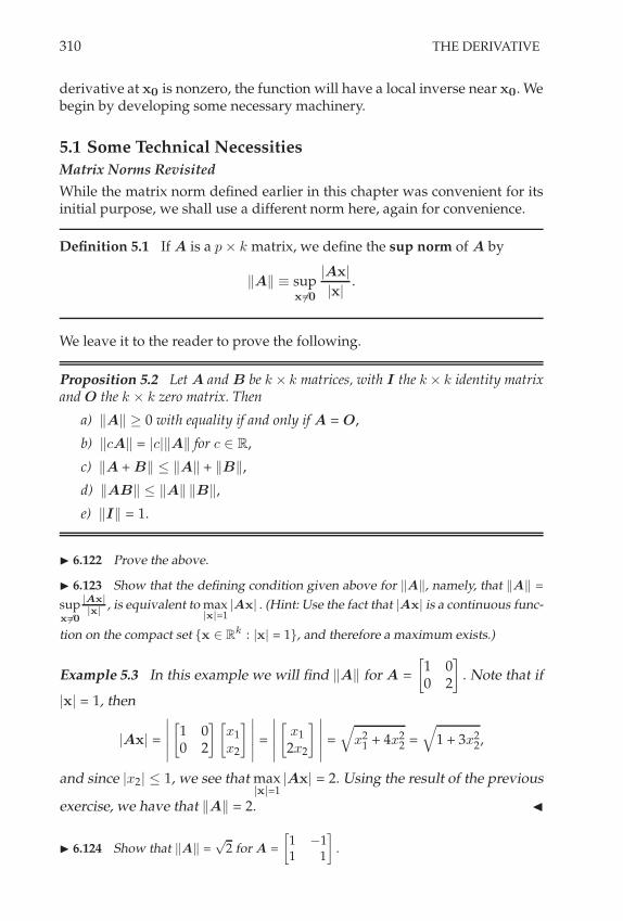
310 THE DERIVATIVE
derivative at x0 is nonzero, the function will have a local inverse near x0. Webegin by developing some necessary machinery.
5.1 Some Technical NecessitiesMatrix Norms Revisited
While the matrix norm defined earlier in this chapter was convenient for itsinitial purpose, we shall use a different norm here, again for convenience.
Definition 5.1 If A is a p . k matrix, we define the sup norm of A by
2A2 / supx,=0
|Ax|
|x|.
We leave it to the reader to prove the following.
Proposition 5.2 Let A and B be k . k matrices, with I the k . k identity matrixand O the k . k zero matrix. Then
a) 2A2 ! 0 with equality if and only if A = O,
b) 2cA2 = |c|2A2 for c # R,
c) 2A + B2 + 2A2 + 2B2,
d) 2AB2 + 2A2 2B2,
e) 2I2 = 1.
! 6.122 Prove the above.
! 6.123 Show that the defining condition given above for 4A4, namely, that 4A4 =
supx(=0
|Ax||x| , is equivalent to max
|x|=1|Ax| . (Hint: Use the fact that |Ax| is a continuous func-
tion on the compact set {x " Rk : |x| = 1}, and therefore a maximum exists.)
Example 5.3 In this example we will find 2A2 for A =
91 00 2
:. Note that if
|x| = 1, then
|Ax| =
&&&&&
91 00 2
: 9x1x2
: &&&&& =
&&&&&
9x1
2x2
: &&&&& =*
x21 + 4x2
2 =*
1 + 3x22,
and since |x2| + 1, we see that max|x|=1
|Ax| = 2. Using the result of the previous
exercise, we have that 2A2 = 2. "
! 6.124 Show that 4A4 =*
2 for A =
91 &11 1
:.

THE INVERSE AND IMPLICIT FUNCTION THEOREMS 311
! 6.125 Show that for a, b " R if A =
9a 00 b
:then 4A4 = max
,|a|, |b|
-.
We now establish that the two matrix norms we have introduced (recall thematrix norm used in Chapter 6) are in fact equivalent. That is, convergencein one implies convergence in the other.
Proposition 5.4 Let A = [aij] be a p . k matrix and recall that |A| = maxi,j
|aij |
where the maximum is taken over all 1 + i + p and 1 + j + k. Then
|A| + 2A2 + k,
p |A|.
PROOF Note that for fixed j such that 1 + j + k, we have
2A2 !
&&Aej
&& =
&&&&&&&
5
V6aij
...apj
7
W8
&&&&&&&!
&&aij
&& for 1 + i + p.
Therefore 2A2 ! |A|, and the left side of the double inequality is established.We will now establish the right side. To do so, note that
|Ax|2 =
&&&&&&&
5
V6a11x1 + · · · + a1kxk
...ap1x1 + · · · + apkxk
7
W8
&&&&&&&
2
= (a11x1 + · · · + a1kxk)2 + · · · + (ap1x1 + · · · + apkxk)2
+
,|a11||x1| + · · · + |a1k||xk |
-2+ · · · +
,|ap1||x1| + · · · + |apk||xk|
-2
+ (k|A| |x|)2 + · · · + (k|A| |x|)2
= pk2|A|
2|x|2,
which implies the right side of the result. #
Once we have the notion of a norm on the set of all p . k matrices we candefine topological properties as well as convergence properties. For example,if {An} is a sequence of p . k matrices then we say lim An = A exists if
(1) A is a p . k matrix,
(2) For all ! > 0 there exists N # N such that n > N ) |An " A| < !.
Proposition 5.4 implies that the convergence of the sequence {An} is inde-pendent of the two norms | · | and 2 · 2.
! 6.126 Show that the convergence referred to above is independent of the twonorms | · | and 4 · 4.
! 6.127 Can you define what it means for;%
j=1 Aj to converge where the Aj arep + k matrices?
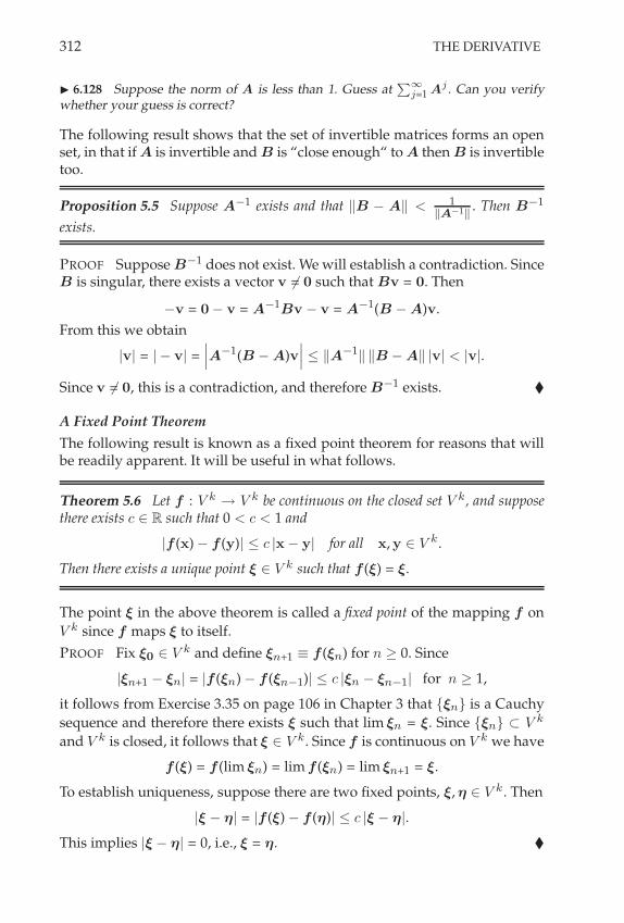
312 THE DERIVATIVE
! 6.128 Suppose the norm of A is less than 1. Guess at;%
j=1 Aj . Can you verifywhether your guess is correct?
The following result shows that the set of invertible matrices forms an openset, in that if A is invertible and B is “close enough“ to A then B is invertibletoo.
Proposition 5.5 Suppose A"1 exists and that 2B " A2 < 1-A"1- . Then B"1
exists.
PROOF Suppose B"1 does not exist. We will establish a contradiction. SinceB is singular, there exists a vector v $= 0 such that Bv = 0. Then
"v = 0" v = A"1Bv " v = A"1(B " A)v.
From this we obtain
|v| = |" v| =&&&A"1(B " A)v
&&& + 2A"12 2B " A2 |v| < |v|.
Since v $= 0, this is a contradiction, and therefore B"1 exists. #
A Fixed Point Theorem
The following result is known as a fixed point theorem for reasons that willbe readily apparent. It will be useful in what follows.
Theorem 5.6 Let f : V k3 V k be continuous on the closed set V k, and suppose
there exists c # R such that 0 < c < 1 and
|f (x) " f (y)| + c |x" y| for all x, y # V k .
Then there exists a unique point ! # V k such that f (!) = !.
The point ! in the above theorem is called a fixed point of the mapping f onV k since f maps ! to itself.
PROOF Fix !0 # V k and define !n+1 / f (!n) for n ! 0. Since
|!n+1 " !n| = |f (!n) " f (!n"1)| + c |!n " !n"1| for n ! 1,
it follows from Exercise 3.35 on page 106 in Chapter 3 that {!n} is a Cauchysequence and therefore there exists ! such that lim !n = !. Since {!n} ' V k
and V k is closed, it follows that ! # V k. Since f is continuous on V k we have
f (!) = f (lim !n) = lim f (!n) = lim !n+1 = !.
To establish uniqueness, suppose there are two fixed points, !, # # V k . Then
|! " #| = |f (!) " f (#)| + c |! " #|.
This implies |! " #| = 0, i.e., ! = #. #

THE INVERSE AND IMPLICIT FUNCTION THEOREMS 313
5.2 The Inverse Function Theorem
With all of the necessary technical results now at our disposal, we may prove,in stages, the inverse function theorem. We begin with the statement of thetheorem.
Theorem 5.7 (The Inverse Function Theorem)Let f : Dk
3 Rk be C1 and suppose f !(a) is invertible for some a # Dk . Then thereexist open sets U ' Dk and V ' Rk with a # U such that f maps U one-to-oneand onto V . Moreover, the function g : V 3 U given by g = f"1 is differentiable
at each y0 # V with g!(y0) =Af !(x0)
B"1 where x0 = g(y0).
The theorem is surprisingly difficult to prove. To do so we will need a seriesof five lemmas, which we now establish. The first one gives a convenientmeans, in a different but equivalent manner to that given in Chapter 6, forcharacterizing when a function is continuously differentiable at a point.
Lemma 5.8 Consider f : Dk3 Rk where f (x) /
,f1(x), f2(x), . . . , fk(x)
-for
fj : Dk3 R. Then f ! is continuous at a # Dk if and only if for any ! > 0 there
exists a . > 0 such that
|x " a| < . ) 2f !(x) " f !(a)2 < !.
PROOF Given any ! > 0, suppose 2f !(x) " f !(a)2 < ! whenever |x" a| < ..Then we have for any 1 + i, j + k that
|x " a| < . )
&&&&*fi
*xj(x) "
*fi
*xj(a)
&&&& + 2f !(x) " f !(a)2 < !,
which implies that all partial derivatives -fi-xj
are continuous at a, and hence
that f ! is continuous at a. Now suppose f is C1 at a # Dk. Then all partial
derivatives -fi-xj
are continuous at a. That is, for any ! > 0 there exists a single
. > 0 (Why?) such that for any 1 + i, j + k we have
|x " a| < . )
&&&&*fi
*xj(x) "
*fi
*xj(a)
&&&& <!
k3/2.
By Proposition 5.4 on page 311 we have
|x " a| < . ) 2f !(x) " f !(a)2 + k3/2 maxi,j
M&&&&*fi
*xj(x) "
*fi
*xj(a)
&&&&
N
< !,
and the result is proved. #
The second lemma establishes a certain topological property about the imageb = f (a) when f !(a) is an invertible matrix.

314 THE DERIVATIVE
Lemma 5.9 Let f : Dk3 Rk be C1 and suppose a # Dk with f (a) = b and
f !(a) invertible. Then b is an interior point to f,Nr(a)
-for every neighborhood
Nr(a) ' Dk .
PROOF Let f !(a) = A and let # = 142A
"12"1. Then there exists . > 0 such
that
x # N+(a) ) |f (x) " f (a) " A(x" a)| + #|x" a| and 2f !(x) " A2 < #.
The first part of above conclusion follows from the differentiability of f ata. The second part of the conclusion follows from Lemma 5.8. Note too thatby Proposition 5.5 on page 312 the function f ! is invertible on all of N+(a).Given the above, we will show that if r + . then Nr.(b) ' f
,Nr(a)
-. To see
this, let y0 # Nr.(b), i.e., |y0 " b| < r#, and let G : Dk3 Rk be given by
G(x) = A"1(y0 " b) " A"1,f (x) " f (a) " A(x " a)-
+ a
= A"1,y0 " f (x)-
+ x. (6.45)
It follows that for x # Nr/2(a) we have
|G(x) " a| + 2A"12 |y0 " b| + 2A"1
2 |f (x) " f (a) " A(x " a)|
< 2A"12 r# + 2A"1
2# |x" a|
< 14 r + 1
412 r < 1
2 r,
that is, G(Nr/2(a)
)' Nr/2(a). Now, from (6.45) we have G!(x) = I"A"1f !(x),
and so2G!(x)2 = 2A"1(A " f !(x))2 + 2A"1
2# = 14 .
By the mean value theorem for functions of several variables, this implies|G(x) " G(a)| + 1
4 |x " a|, and so G has a fixed point x0 # Nr/2(a). From(6.45), this fixed point has the property that
y0 = f (x0) # f,Nr/2(a)
-' f
,Nr(a)
-,
and the lemma is established if r + .. Finally, if r > . we have N+.(b) '
f,N+(a)
-by the argument just established, and clearly f
,N+(a)
-' f
,Nr(a)
-.
Overall then we have shown that N+.(b) ' f,Nr(a)
-and the lemma is
proved. #
The third lemma gives sufficient conditions under which f : Dk3 Rk is
one-to-one at and near a # Dk .
Lemma 5.10 Let f : Dk3 Rk be C1 and suppose f !(a) is invertible for some
a # Dk. Then there exists . > 0 such that f is one-to-one on N+(a).
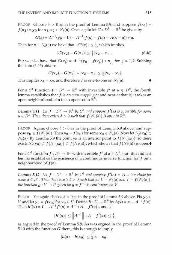
THE INVERSE AND IMPLICIT FUNCTION THEOREMS 315
PROOF Choose . > 0 as in the proof of Lemma 5.9, and suppose f (x1) =f (x2) = y0 for x1, x2 # N+(a). Once again let G : Dk
3 Rk be given by
G(x) = A"1(y0 " b) " A"1(f (x) " f (a) " A(x " a)) + a.
Then for x # N+(a) we have that 2G!(x)2 +14 , which implies
|G(x2) " G(x1)| + 14 |x2 " x1| . (6.46)
But we also have that G(xj) = A"1,y0 " f (xj)
-+ xj for j = 1, 2. Subbing
this into (6.46) obtains
|G(x2) " G(x1)| = |x2 " x1| +14 |x2 " x1|.
This implies x1 = x2, and therefore f is one-to-one on N+(a). #
For a C1 function f : Dk3 Rk with invertible f ! at a # Dk, the fourth
lemma establishes that f is an open mapping at and near a; that is, it takes anopen neighborhood of a to an open set in Rk .
Lemma 5.11 Let f : Dk3 Rk be C1 and suppose f !(a) is invertible for some
a # Dk. Then there exists . > 0 such that f,N+(a)
-is open in Rk.
PROOF Again, choose . > 0 as in the proof of Lemma 5.9 above, and sup-pose y0 # f
,N+(a)
-. Then y0 = f (x0) for some x0 # N+(a). Now let N%(x0) '
N+(a). By Lemma 5.9 the point y0 is an interior point to f,N%(x0)
-, so there
exists Ns(y0) ' f,N%(x0)
-' f
,N+(a)
-, which shows that f
,N+(a)
-is open.#
For a C1 function f : Dk3 Rp with invertible f ! at a # Dk , our fifth and last
lemma establishes the existence of a continuous inverse function for f on aneighborhood of f (a).
Lemma 5.12 Let f : Dk3 Rk be C1 and suppose f !(a) = A is invertible for
some a # Dk . Then there exists . > 0 such that for U = N+(a) and V = f,N+(a)
-,
the function g : V 3 U given by g = f"1 is continuous on V .
PROOF Yet again choose . > 0 as in the proof of Lemma 5.9 above. Fix y0 #
V and let y0 = f (x0) for x0 # U . Define h : U 3 Rk by h(x) = x " A"1f (x).Then h!(x) = I " A"1f !(x) = A"1
,A " f !(x)
-, and so
2h!(x)2 +
XXXA"1XXX 2A " f !(x)2 +
14 ,
as argued in the proof of Lemma 5.9. As was argued in the proof of Lemma5.10 with the function G there, this is enough to imply
|h(x) " h(x0)| + 14 |x " x0|.

316 THE DERIVATIVE
But we also have
|h(x) " h(x0)| =&&&(x" x0) " A"1(f (x) " f (x0))
&&& ,
from which the reverse triangle inequality obtains
|x " x0| +43 2A
"12 |f (x) " f (x0)| ,
and if we let x = g(y), we get
|g(y) " g(y0)| + 43 2A
"12 |y " y0| . (6.47)
This last expression implies that g is (Lipschitz) continuous. #
We are now ready to prove the inverse function theorem.
PROOF (of the inverse function theorem)
We assume that f : Dk3 Rk is C1 and that f !(a) is invertible for some a #
Dk . Let U = N+(a) with . > 0 as chosen in the proofs of the previous lemmas,and let V = f
,N+(a)
-. For any y0 = f (x0) # V we will show that g : V 3 U
given by g = f"1 is differentiable at y0 and that g!(y0) =Af !(x0)
B"1. To thisend, let ! > 0 and fix y0 # V . Let f !(x0) = A. By Lemma 5.12 we have thatg : V 3 U given by g = f"1 is continuous on V . For y # V with g(y) = x, let! > 0 be given. Then there exists .1 > 0 such that if |x " x0| < .1 we have
&&&g(y) " g(y0) " A"1(y " y0)&&& =
&&&x " x0 " A"1(f (x) " f (x0))&&&
=&&&A"1(f (x) " f (x0) " A(x " x0))
&&&
+ 2A"12
34 !
2A"12
2|x " x0|
= 34 !
1
2A"12
|g(y) " g(y0)|
+ ! |y " y0|. (6.48)
The first inequality in the above follows from the differentiability of f at x0,while the second follows from (6.47) in the proof of Lemma 5.12. Note that|x " x0| < .1 if and only if |g(y) " g(y0)| < .1, which will be true if
43 2A2 |y " y0| < .1,
i.e., if |y" y0| < . /34
1-A-.1. We have shown that if y is within . of y0, then
(6.48) holds, and therefore g is differentiable at y0 # V with g!(y0) = A"1 =Af !(x0)
B"1. #
It will be convenient to have the differentiability of the inverse function of acomplex differentiable function. Fortunately, this is a simple corollary of theresult already proved.

THE INVERSE AND IMPLICIT FUNCTION THEOREMS 317
Theorem 5.13 Suppose f : D 3 C is differentiable with f &(a) $= 0. Then thereexist open sets U ' D, and V ' C such that a # U , and such that f maps Uone-to-one and onto V . Moreover, the function g : V 3 U given by g = f"1 isdifferentiable at each w0 # V with g&(w0) = (f &(z0))"1 where z0 = g(w0).
PROOF Writing z0 = x0 + iy0 and f = u + iv, and noting that f &(z0) =ux(x0, y0) + ivx(x0, y0) $= 0, we have by the Cauchy-Riemann equations
ux(x0, y0) = vy(x0, y0) $= 0 and uy(x0, y0) = "vx(x0, y0) $= 0.
Now consider f as a function f : R23 R2. Then the Jacobian matrix of f at
(x0, y0) is
J(x0, y0) =
5
6ux(x0, y0) uy(x0, y0)
vx(x0, y0) vy(x0, y0)
7
8 ,
whose determinant is u2x(x0, y0) + u2
y(x0, y0) > 0, and so J(x0, y0) is invert-ible. We thus know, by the inverse function theorem, that there are open setsU , V ' R2 such that f maps U onto V in a one-to-one correspondence andsuch that the inverse g is continuously differentiable as a real function. Weneed to show that it is also differentiable as a complex function, i.e., that itsatisfies the Cauchy-Riemann equations. We know that f &(z0) is of the form
9A B
"B A
:with A2 + B2 > 0,
and we must show that its inverse matrix, which is the derivative of f"1 atf (z0), is of that same form. This will show that the inverse function satisfiesthe Cauchy-Riemann equations. But this can be seen directly; the inverse isgiven by 1
A2 + B2
9A "BB A
:,
and so clearly the inverse of f satisfies the Cauchy-Riemann equations. Bythe inverse function theorem the inverse is differentiable, and therefore con-tinuous, and so A and B in the above matrix expression are continuous par-tial derivatives. Therefore, going back to the complex plane, the inverse g off is complex differentiable with the appropriate derivative, and the proof iscomplete. #
Corollary 5.14 Suppose f : D 3 C is differentiable on the open set D ' C.Suppose that f (D) = V is open and f is one-to-one, and suppose f & does not vanish.Then the inverse map g = f"1 : V 3 D is also differentiable.
PROOF By the previous theorem, g is differentiable in a neighborhood ofeach point, and since g may be defined everywhere since f is a one-to-onecorrespondence, g is also differentiable everywhere. #

318 THE DERIVATIVE
Some examples will illustrate the inverse function theorem’s implicationsand limitations.
Example 5.15 Let f : R 3 R be given by f (x) = x2. Then if a $= 0 wehave f &(a) $= 0 and therefore there exists a neighborhood Nr(a) such thatf : Nr(a) 3 V is one-to-one and onto, and f"1 : V 3 Nr(a) is differen-tiable on V . Moreover,
,f"1
-&(b) = 1
f !(a) where f (a) = b. In fact, if a > 0, theneighborhood Nr(a) can be replaced by the interval (0,-). That is, an inversefunction for f with the stated properties exists on all of (0,-). Likewise, onecan find an inverse for f with the stated properties on all of ("-, 0). But onecannot find a single inverse for f with all the stated properties on all of R. "
! 6.129 What are the inverse functions defined on (0, /) and (&/, 0) referred to inthe above example?
Example 5.16 Maps that are “dimension reducing“ are not invertible any-where. To see an example of this, let f : R2
3 R2 be given by f (x, y) =(sec xy, tan xy). We will show that f is not invertible in a neighborhood ofany point. To see this, note that
f !(x, y) =
5
6y sec xy tan xy x sec xy tan xy
y sec2 xy x sec2 xy
7
8 ,
and det,f !
-(x, y) = xy sec3 xy tan xy"xy sec3 xy tan xy / 0 for every (x, y) #
R2. In this case, where f ! is singular, the function f effectively maps theset R2 to a curve, a set of lower dimension. To see this, let u = sec xy andv = tan xy. Then for all (x, y) # R2 we have f (x, y) = (u, v) where u2
" v2 = 1.Therefore f takes all points in the plane to the points on a hyperbola in theplane. "
! 6.130 Let f : R2 , R
2 be given by f (x, y) = (x2 + xy, x2 + y2) = (u, v).
a) At which points in R2 can you find an inverse for this mapping?
b) Describe the set of points where no inverse to this mapping exists.
Example 5.17 Let f : C 3 C given by f (z) = ez. Then for every a # C, wehave f &(a) = ea
$= 0. Therefore there exists a neighborhood Nr(a) such thatf : Nr(a) 3 V is one-to-one and onto, and the inverse function f"1 : V 3
Nr(a) is differentiable on V . Note that f"1 is a logarithm of z defined on V .
Moreover,,f"1
-&(w) = 1f !(a) = 1
ea = 1w where ea = w. "
! 6.131 For a given nonzero a " C, what is the inverse of f referred to in the previ-ous example? What is its domain? What if a is replaced by &a? What if a = 0?
5.3 The Implicit Function Theorem
Suppose we have an equation in two variables F (x, y) = 0, and that the pair(x, y) = (a, b) is a solution. It is convenient to be able to solve the equation

THE INVERSE AND IMPLICIT FUNCTION THEOREMS 319
F (x, y) = 0 for y as a function of x, say y = h(x), near (a, b) such that F (x, y) =F (x, h(x)) = 0. The implicit function theorem tells us that under the rightconditions we can do this locally, even in higher dimensions. Before statingand proving the theorem, however, we introduce some helpful notation andmake some preliminary comments.
Notation
Suppose x = (x1, x2, . . . , xk) # Rk and y = (y1, y2, . . . , yl) # Rl. Then we write(x, y) / (x1, x2, . . . , xk , y1, y2, . . . , yl) # Rk+l, and thus identify Rk+l with theCartesian product Rk
. Rl. If (x, y) # Rk+l, we will assume that x # Rk andthat y # Rl unless otherwise noted. For two sets A ' Rk and B ' Rl, wewrite A . B / {(x, y) : x # A, y # B}.
! 6.132 Show that (x1 + x2, y) = (x1, y) + (x2, y). Also, show that a similar identityholds for scalar products. If A+B = !, then what are A and B? What if A+B = R
k+l?
Finally, suppose we are given a differentiable F : Dk+l3 Rl, with F =
(F1, . . . , Fl) and Fi : Dk+l3 R for 1 + i + l. The derivative F &(x, y) is given
by the usual matrix:
F &(x, y) =
5
VVVVVVVV6
-F1-x1
. . . -F1-xk
-F1-y1
. . . -F1-yl
-F2-x1
. . . -F2-xk
-F2-y1
. . . -F2-yl
.... . .
......
. . ....
-Fl-x1
. . . -Fl-xk
-Fl-y1
. . . -Fl-yl
7
WWWWWWWW8
(The only difference is that there are entries for both the x and y coordinates.)Define the matrix Fx by
Fx /
5
VVVVVVVV6
-F1-x1
-F1-x2
. . . -F1-xk
-F2-x1
-F2-x2
. . . -F2-xk
......
. . ....
-Fl-x1
-Fl-x2
. . . -Fl-xk
7
WWWWWWWW8
,
and similarly for Fy. This notational convention allows us to write
F &(x, y) =AFx Fy
B.
! 6.133 Show that all the standard linearity properties hold for Fx and Fy. Whatabout a function F : D
k+l+m , Rl given by F (x,y, z) in three variables? Define
what (x, y, z) means and define the expressions Fx, Fy, and Fz.

320 THE DERIVATIVE
The Implicit Function Theorem
We now use the above-developed notation to state and prove the implicitfunction theorem, which itself is an application of the inverse function theo-rem. Our proof of the result is from [Rud76].
Theorem 5.18 (The Implicit Function Theorem)Suppose F : Dk+l
3 Rl is continuously differentiable on the open set Dk+l' Rk+l.
Suppose (a, b) # Dk+l satisfies F (a, b) = 0. Assume, moreover, that the squarematrix Fy(a, b) is invertible. Then there exists a neighborhood Nr(a) of a and acontinuously differentiable function h : Nr(a) 3 Rl satisfying h(a) = b such thatif x # Nr(a), then F (x, h(x)) = 0. Moreover, on Nr(a) we have
h&(x) = "
AFy(x, h(x))
B"1Fx(x, h(x)).
PROOF Consider the function G : Dk+l3 Rk+l given by G(x, y) = (x, F (x, y)).
Then we have G(a, b) = (a, F (a, b)) = (a, 0). The definition of G makes it clearthat if the output of G has the second coordinate zero, then the input repre-sents a solution of F (x, y) = 0. Hence it is for such points that we search. Todo this, we will apply the inverse function theorem to G. Note that
G&(a, b) =
5
6I O
Fx(a, b) Fy(a, b)
7
8 , (Why?)
with all partial derivatives evaluated at (a, b). On the right, we have writtenthe matrix in what is often referred to as “block form,“ with I representingthe k.k identity matrix and O representing the l.l zero matrix. We assumedthat Fy(a, b) was invertible, and obviously I is invertible. We now use a factfrom linear algebra, namely, if a matrix is given in block form
M =
9A OB C
:,
where A and C are square matrices, then det M = det A det C. In particu-lar, M is invertible if and only if A and C are. This obtains that G&(a, b) isinvertible. Since F is continuously differentiable it follows that G is contin-uously differentiable, and therefore the inverse function theorem applies toG. Let U ' Dk+l and V ' Rk+l be open sets such that (a, b) # U and (a, 0) =F (a, b) # V . Then G : U 3 V has inverse function G"1 : V 3 U , which isdifferentiable on V . Since V is open, there exists N%(a, 0) ' V . We leave it tothe reader to show that there exists Nr1 (a) ' Rk and Nr2(0) ' Rl such that(a, 0) # Nr1 (a).Nr2 (0) ' N%(a, 0) ' V . It follows that there exists a functionH : V 3 U differentiable on V such that G"1(x, y) = (x, H(x, y)). If we leth : Nr1 (a) 3 Rl be given by the differentiable function h(x) = H(x, 0). Thenthe function h has the desired property that we seek, namely, for x # Nr1 (a)

SUPPLEMENTARY EXERCISES 321
we have
(x, 0) = G(G"1(x, 0)) = G(x, H(x, 0)) = G(x, h(x)) =,x, F (x, h(x))
-.
This means that F (x, h(x)) = 0 on Nr1 (a). Finally, we leave it to the reader toverify that
0 = F !(x, h(x))
9I
h&(x)
:
=AFx(x, h(x)) Fy(x, h(x))
B 9I
h&(x)
:
= Fx(x, h(x)) + Fy(x, h(x))h&(x).
This implies that
h&(x) = "
AFy(x, h(x))
B"1Fx(x, h(x)),
and the theorem is proved. #
! 6.134 Answer the (Why?) question in the above proof. Also, given a neighborhood
N)(x0, y0) ! Rk+l, show that it contains a product of two neighborhoods Nr1 (x0) +
Nr2 (y0).
Example 5.19 Consider the system of equations given by
3x + 6y + z3 = 0
x + 2y + 4z = 0.
We will show that it is possible to solve this system of equations for x and zin terms of y. To do so, let f : R3
3 R2 be given by f (x, y, z) = (3x + 6y +
z3, x + 2y + 4z). Then f !(x, y, z) =
93 3z2 61 4 2
:. Since f (0, 0, 0) = (0, 0), we
examine f !(0, 0, 0) =
93 0 61 4 2
:. Since
93 01 4
:is invertible, we may solve
for y in terms of x and z. "
! 6.135 In the above example, can we solve for z in terms of x and y?
6 SUPPLEMENTARY EXERCISES
1. Consider the function f : R , R given by f (x) = 2x2 & 3. Use the $, . version of
derivative to show that f#(1) %= 3. Hint: Use the method of proof by contradiction.
2. Let f : R , R be given by f (x) =
Ex
2 for x irrational
0 for x rational. Find the points
x " R where f is differentiable.
3. Can you find a function f : R , R that is differentiable at exactly two points?

322 THE DERIVATIVE
4. The function f : R , R given by f (x) = |x| is differentiable everywhere in R exceptat x = 0. Can you find a function f : R , R that is differentiable everywhere exceptat exactly two points?
5. For a fixed positive integer N , show that the function f : R , R given by f (x) =;N
j=1 |x& j| is differentiable everywhere in R except at x = j for j = 1, 2, . . . , N . Whatif each of the points x = j is replaced by a more generic xj " R?
6. Consider the function f : R , R given by f (x) =;%
j=0|x!j|
j! . Show that f isdifferentiable everywhere in R except at j = 0, 1, 2, . . . .
7. Recall from a previous exercise that f : R , R is called Lipschitz continous if thereexists a nonnegative real number M independent of x and y where
|f (x) & f (y)| # M |x & y| for all x, y " R.
Is a function that is Lipschitz continuous on R necessarily differentiable on R? Is afunction that is differentiable on R necessarily Lipschitz continuous on R?
8. Suppose f : R , R is such that there exists a nonnegative real number M and apositive real number $ each independent of x and y where
|f (x) & f (y)| # M |x & y|1+$ for all x, y " R.
Show that f is differentiable on R. Can you say anything else about f?
9. Consider f : D1 , R and interior point x0 " D
1. Suppose that
limx#x0x!Q
f (x) & f (x0)x & x0
exists. That is, for any sequence of rational x that converges to x0, the limit of thedifference quotient always gives the same finite value. Show by counterexample thatdespite this, f
#(x0) does not necessarily exist.
10. Suppose f : D1 , R is given by f (x) = tan x where
D1 =
!x " R : x %= 2n+1
2 ' for n " Z
". Show that f
#(a) = sec2a for all a " D
1. Use
the quotient rule to find the derivative for each of the functions sec x, csc x, and cot x,remembering to specify each on its appropriate domain.
11. Consider the function f (x) : (&1, 1) , R given by f (x) = x2/3. What is the domain
of f#(x)?
12. For the following functions, find the local extrema and determine their nature asin Example 1.15 on page 248.
a) f (x) = 14 x
4 & x3 + 3
2 x2 & x & 5, x " R b) f (x) = x
x+1 , x " [1, 4]
c) f (x) = x2!1
x2+1 , x " R d) f (x) = x"2& sin x, x " [0, ')
13. Consider the function f : [&1, 1] , R given by f (x) = |x|. Find and characterizeany extrema. Does this example contradict Corollary 1.14?

SUPPLEMENTARY EXERCISES 323
14. We used Rolle’s theorem to prove the mean value theorem. See if you can use themean value theorem to prove Rolle’s theorem instead.
15. Why do you suppose Theorem 1.17 is called the mean value theorem?
16. Suppose f : (a, b) 0 (c, d) , R is differentiable on the disjoint union (a, b) 0 (c, d),and f
#(x) = 0 for all x " (a, b) 0 (c, d). Is it still true that there exists a constant c suchthat f (x) . c for all x " (a, b) 0 (c, d)? What if c = b?
17. As students of calculus are well aware, the second derivative test can be of greatpractical value in determining the nature of a critical point. If the critical point corre-sponds to an extrema of the function f , the second derivative test described below candetermine whether it is a local minimum or a local maximum. Of course, not all crit-ical points correspond to extrema, as the example of x = 0 for the function f (x) = x
3
illustrates. In this case, x = 0 corresponds to an inflection point, a point where theconcavity of the curve associated with the graph of f (x) in the xy-plane changes sign.At such points, the second derivative test is inconclusive. Use the mean value theo-rem to prove the following:
Suppose f : Nr(a) , R for some r > 0 is such that f## exists and is
continuous on Nr(a), and f#(a) = 0.
a) If f##(a) > 0, then f (a) is a local minimum.
b) If f##(a) < 0, then f (a) is a local maximum.
c) If f##(a) = 0, the test is inconclusive.
18. Prove the following: If f : (a, b) , R is differentiable, then at each x " (a, b),the derivative f
# is either continuous or has an essential discontinuity, i.e., f# has no
removable or jump discontinuities.
19. Consider the function f : R , R given by f (x) =
E1
24 x4 for x ' 0
& 124 x
4 for x < 0.
a) Find the highest possible degree Taylor polynomial at x = 0 having a remainderaccording to Theorem 1.22.
b) What is the expression for its remainder term?
c) Suppose you are interested in evaluating f (x) at x = & 12 via your Taylor
approximation with remainder as described by your results from parts a)and b). How small might the remainder be? How large? Can you make itarbitrarily small?
d) Suppose you are interested in evaluating f (x) at x = 12 via your Taylor
approximation with remainder as described by your results from parts a)and b). How small might the remainder be? How large? Can you make itarbitrarily small?
20. Suppose f and g are differentiable on N#r(a) ! R for some r > 0 such that the
following all hold:

324 THE DERIVATIVE
(i) limx&a f (x) = limx&a g(x) = ±/(ii) g
#(x) %= 0 for all x " N#r(a)
(iii) limx&af%(x)
g%(x) = L exists
Prove that limx&af (x)g(x) = L.
21. For the following functions, find the largest n for which f " Cn(D1).
a) f (x) = x!1, D
1 = (0, 2) b) f (x) = |x|, D1 = (&1, 0)
c) f (x) = |x|, D1 = (&1, 1) d) f (x) = x
x2+1 , D1 = R
e) f (x) = sin(x
2)
, D1 = R f ) f (x) =
Ex
2/2 if x ' 0
&x2/2 if x # 0
, D1 = R
22. Let fn : R , R be given by fn(x) =
RT
Ux
n sin(
1x
)x %= 0
0 x = 0.
a) Show that f1 is continuous, but not differentiable at x = 0.
b) What can you say about f2?
c) What can you say about fn?
23. Let f : [0, /) , R be given by f (x) =*
x. Find Df % .
24. Let f : R , R be given by f (x) = |x|. Find Df % .
25. Let f : R , R be given by f (x) =
Ex
2 if x # 0
x if x > 0. Find Df % and Df %% .
26. Discuss the critical point of the function f : [&1, 1] , R given by f (x) = x2/3.
Does the (interior) minimum happen at a point where f# = 0? Does this example
contradict Corollary 1.14 on page 248?
27. Consider f : R , R given by f (x) =
RT
Ux
2 sin(
1x
)if x %= 0
0 if x = 0.
a) Show that f is differentiable on R, and that f#(0) = 0. Therefore x = 0 is a critical
point.
b) Show that f#(x) is discontinuous at x = 0.
c) Show that f#(x) takes values that are greater than 0 and less than 0 in any neigh-
borhood of x = 0, and hence x = 0 is not a local extremum.
d) Show that f##(0) doesn’t exist, and so x = 0 is not an inflection point.
28. Confirm that f : R , R given by f (x) =
RT
Ux
4 sin(
1x
)if x %= 0
0 if x = 0has the prop-
erty that f#(0) = f
##(0) = 0, but x = 0 is not an extremum or an inflection point.

SUPPLEMENTARY EXERCISES 325
29. Consider the function f : R , R given by f (x) =
RT
U
x
2 + x2 sin
(1x
)for x %= 0
0 for x = 0.
a) Show that f is differentiable in a neighborhood of x = 0, and that f#(0) is
positive.
b) Can you find an interval containing x = 0 throughout which f is increasing?
c) Find a . > 0 such that f (x) < 0 on (&., 0) and f (x) > 0 on (0, .).
30. Consider f : R , R given by f (x) =
Ex
2 if x # 2
ax + b if x > 2where a and b are
constants. Can you find values of a and b that make f# continuous on R?
31. Suppose f : R , R has the following properties.
a) f is continuous at x = 0,
b) f (a + b) = f (a) + f (b) for all a, b " R,
c) f#(0) = C for some constant C.
Show that f (x) = Cx for all x " R.
32. For f : R , R given by f (x) =
Ee!1/x if x > 0
0 if x # 0find f
#(x) and f##(x) for all
x " R.
33. Suppose f : (a, b) , R is differentiable on (a, b). Find a nonconstant sequence{xn} ! (a, b) satisfying both of the following (Hint: Use the mean value theorem.):
a) lim xn = c " (a, b),
b) lim f#(xn) = f
#(c).
34. Suppose f : R , R is differentiable at the point x0. Compute
limh&0
f (x0 + ! h) & f (x0 + " h)h
where ! and " are constants.
35. Can you use the Cauchy mean value theorem on page 250 to prove the meanvalue theorem?
36. Consider f : R , R and suppose there exists some constant K " R such thatfor all x and y in R, |f (x) & f (y)| # K (x & y)2. Prove that there exists some constantc " R such that f . c on R.
37. In the previous exercise, what if the exponent 2 is replaced by !? For what valuesof ! does the conclusion still hold?
38. Let a1, . . . , an be a set of nonnegative real numbers. The arithmetic-geometricmean inequality states that the arithmetic mean is at least the geometric mean, i.e.,
1n
n+
j=1
aj ' (a1 . . . an)1/n.

326 THE DERIVATIVE
The inequality is obvious if one of the ajs is zero, so assume all of them are nonzero.
a) Let c > 0. If the inequality is true for a1, . . . , an, then it is true for ca1, . . . , can. Thusshow that it is enough to consider the case when a1 . . . an = 1, so the geometricmean is 1.
b) Let x > 0. Prove that x & 1 ' log x. Use the mean value theorem, considering thecases x > 1, x < 1, and x = 1 separately.
c) Now suppose a1 . . . an = 1. Use the previous inequality to get
n+
j=1
aj & n ' 0, hence1n
n+
j=1
aj ' 1.
This proves the inequality. This proof, due to Schaumberger, is from [Sch85].
39. Consider f : R , R such that limx&% f (x) = /.
a) Can you find a function h : R , R such that limx&% h(x) = /, and for any
integer k ' 1 limx&%A,
f (x)-1/k,
h(x)-!1B
= /?
b) Can you find a function H : R , R such that limx&% H(x) = /, and for any
integer k ' 1 limx&%AH(x)
,f (x)
-!kB= /?
40. Suppose f : R , R is C2 on its whole domain. Show that for any h > 0 and any
x there exists a point # between x & h and x + h such that
f (x + h) & 2 f (x) + f (x & h)
h2= f
##(#).
41. Find the positive real values x for which sin x ' x & x3
6 .
42. Suppose f : R , R is continuously differentiable on R, and assume a < b suchthat
(i) f (b) ' f (a) > 0(ii) f and f
# never have the same sign at any point in [a, b].
Show that there exists a constant c such that f (x) = c on [a, b].
43. Suppose f : R , R is continuously differentiable on R and that f# is never zero
at the roots of f . Show that any bounded interval [a, b] contains no more than a finitenumber of roots of f .
44. Suppose f and g : R , R are differentiable on R such that f g# & f
#g %= 0 on R. If
r1 and r2 are consecutive roots of f , show there is a root of g between r1 and r2.
45. Suppose in the previous exercise that f# and g
# are also continuous. Show thatthere is only one root of g between r1 and r2.
46. Suppose f : R , R is differentiable on R, and assume a < b such that f#(a) < 0 <
f#(b). Show that there exists a number c between a and b such that f
#(c) = 0. (Notethat f
# need not be continuous!)
47. Determine whether the following limit exists: limx&0 x e1/x.

SUPPLEMENTARY EXERCISES 327
48. Show that 120 # x
16+x3 # 112 for 1 # x # 4.
49. Suppose f : [a, b] , R is continuous on [a, b] and differentiable on (a, c) 0 (c, b)for some c " (a, b). Also, suppose limx&c f
#(x) = L. Use the mean value theorem toshow that f
#(c) = L.
50. Establish the following inequalities for nonnegative values of x.
a) e!x # 1 b) 1 & x # e
!xc) e
!x # 1 & x + x2
2Determine a general rule consistent with the above, and prove it.
51. Consider a differentiable function f : [0, /) , R such that limx&% f (x) = M
and limx&% f#(x) = L. Can you use the mean value theorem to determine L?
52. Consider the function f : R\{0} , R given by f (x) = x
1+e1/x . Can you extend thisfunction’s domain to include x = 0? Is f differentiable there? (Hint: Use one-handedlimits.)
53. Suppose fn : [0, 1] , R is given by fn(x) = 1n
e!n
2x
2
for n = 1, 2, . . . .a) Show that the sequence of functions {fn} converges uniformly on [0, 1].
b) Is the same true for the sequence {f #n}? Why or why not?
54. Suppose f : R , R and g : R , R are C1(&/, /), and that g(x) > 0 for all x.
For each real number # define the function W* : R , R by
W*(x) = g(x)f #(x) & # f (x)g#(x).
If a and b are consecutive zeros of the function f , show that for each real number #
the function W* has a zero between a and b.
55. Suppose f : R , R is differentiable on R, and that f#(a) < 0 < f
#(b) for somea < b. Show that there exists c " (a, b) such that f
#(c) = 0 even though f# is not
necessarily continuous.
56. In a supplementary exercise from the previous chapter, we considered the func-
tion f : R , R given by f (x) =;%
j=0|x!j|
j! . There, you were asked to show that thisfunction is well defined, i.e., converges, for any x " R, and that f is continuous onR. Show that this function is differentiable at any x %= N " Z. To get started, what isthe derivative of f at x " (N , N + 1) for N " Z? Compare it to the derivative of f atx " (N & 1, N ).
57. Consider the function f : R \ {0} , R given by f (x) = (cos x)1/x . Can f beassigned a value at x = 0 so as to be continuous there?
58. A Continuous Nowhere Differentiable Function.Such “pathological“ functions are actually more typical than originally realized. Infact, if C[a, b] is the space of continuous functions on the interval [a, b], and if CND[a, b]is the subset of continuous nowhere differentiable functions on [a, b], one can showthat CND[a, b] is dense in C[a, b] when C[a, b] is viewed as a normed complete vectorspace with the sup norm. That is, every continuous function in C[a, b] has a contin-uous nowhere differentiable function arbitrarily near to it. Also, CND[a, b] functions

328 THE DERIVATIVE
are what is known as “prevalent“ in C[a, b], a measure-theoretic concept meaningroughly that “almost all“ functions in C[a, b] are, in fact, members of CND[a, b]. Thatis, they are to C[a, b] what the irrationals are to R! While there are many examplesof functions that are continuous everywhere and differentiable nowhere on their do-mains, one of the earliest examples known was constructed by Bolzano in the 1830s.A more famous example was constructed by Weierstrass some 40 years later. The rel-atively recent example presented here is by McCarthy (published in the AmericanMathematical Monthly, Vol. LX, No.10, December 1953). It has the benefit of simplic-ity over its historical predecessors. Our presentation is inspired by [Thi03]. Define thefunction f : R , R according to
f (x) =%+
k=1
2!k&,22k
x-,
where & : R , R is the “saw-tooth“ function with period 4 given by
&(x) =
E1 + x for x " [&2, 0]
1 & x for x " [0, 2],
and &(x + 4) = &(x) for all x " R.
a) Use the Weierstrass M-test to see that f is continuous on R.b) To show that f is nowhere differentiable, fix an arbitrary x " R. We will construct a
sequence {xn} of real numbers approaching x such that the limit limn&%
|f (xn)!f (x)||xn!x|
does not exist. To this end, let xn = x ± 2!2n
where the sign is selected so that xn
and x are on the same straight-line segment of the saw-tooth function &. Show thefollowing:1. For k " N such that k > n, &
,22k
xn
-& &
,22k
x-
= 0.
2. For k " N such that k = n,&&&
,22k
xn
-& &
,22k
x-&& = 1.
3. For k " N such that k < n, supk${1,2,...,n!1}
&&&,22k
xn
-& &
,22k
x-&& # 2!2n"1
.
c) Show that
|f (xn) & f (x)||xn & x|
= 22n&&&&
%+
k=1
2!k0&,22k
xn
-& &
,22k
x-1&&&&
' 22n2
1 &
&&&&&
n!1+
k=1
2!k0&,22k
xn
-& &
,22k
x-1&&&&
D
' 22n,1 & (n & 1)2!2n"1-
' 22n,1 & 2n2!2n"1-
, which goes to / as n , /.
59. For each of the following functions, use the $, . definition to verify that the deriva-tive is as claimed.a) Consider the function f : D
2 , R with D2 = {(x, y) " R
2 : xy ' 0} and f
given by f (x, y) =*
2xy. At the point (1, 1), show that f has the derivativeA 1"2
1"2
B.
b) Consider the function f : D2 , R with D
2 = {(x, y) " R2 : xy %= 0} and f
given by f (x, y) = (xy)!1. At the point (1, 1), show that f has the derivative
[&1 & 1] .
c) Consider the function f : D3 , R with D
3 = {(x, y, z) " R3 : x + y + z %= 0}

SUPPLEMENTARY EXERCISES 329
and f given by f (x, y) = x
x+y+z. At the point (0, 0, 1), show that f has derivative
given by [1 0 0] .
60. Can you construct a function f : R2 , R that is differentiable at exactly one
point? Exactly two points?
61. Can you construct a function f : R2 , R that is differentiable everywhere on its
domain except at exactly one point? Exactly two points?
62. Show that the function f : R2 , R given by f (x, y) = 4x
2 + xy + y2 + 12 in
Example 2.16 on page 271 is, in fact, differentiable on its whole domain.
63. For the following functions, find all extrema and determine their nature.a) f (x, y) = x
3/3 & x
2y + xy
2 + y2/2, (x, y) " R
2
b) f (x, y) = sin(xy), (x, y) " R2
64. Just as in the case of f : D1 , R, a critical point for a function f : D
2 , R
might not correspond to a local extremum. Such a point in the higher-dimensionalcase might be what is called a saddle point, a higher-dimensional analog of the one-dimensional inflection point. A saddle point corresponding to a function f : D
2 , R
can be defined as a critical point that is neither a local maximum nor a local minimum.Along at least one direction of approach to the saddle point, the behavior is that of alocal minimum, while along at least one other direction the behavior is that of a localmaximum. A simple example of such a saddle point is the origin corresponding tothe graph of the function f : R
2 , R given by f (x, y) = y2 &x
2. For f : R2 , R given
by f (x, y) = y2 & x
2, find a direction along which f attains what appears to be a localminimum as you approach (0, 0). Similarly, find a direction along which this functionattains what appears to be a local maximum as you approach (0, 0).
65. As we have already seen in the case of f : D1 , R, determining the type of
extremum associated with a given critical point is often made easier by applying asecond derivative test. We now describe such a test for the special case of functionsf : D
2 , R. Implementation of the test in this case involves a function D : D2 , R
called the discriminant of f , a function not referred to in the case of f : D1 , R. In
particular, we define D(x) to be the determinant of the two-by-two array of second-order partial derivatives of f evaluated at x, i.e.,
D(x) .
&&&&&&
fxx(x) fxy(x)
fyx(x) fyy(x)
&&&&&&= fxx(x)fyy(x) & fxy(x)fyx(x).
Our test is then stated as follows:
Consider f : D2 , R and suppose a is an interior point of D
2 such thatf !(a) = 0. Suppose also that fxx, fxy , fyx, and fyy exist and are continuouson Nr(a) for some r > 0.
a) If D(a) > 0 and fxx(a) > 0, then f (a) is a local minimum.
If D(a) > 0 and fxx(a) < 0, then f (a) is a local maximum.
b) If D(a) < 0, then a corresponds to a saddle point of the function f .
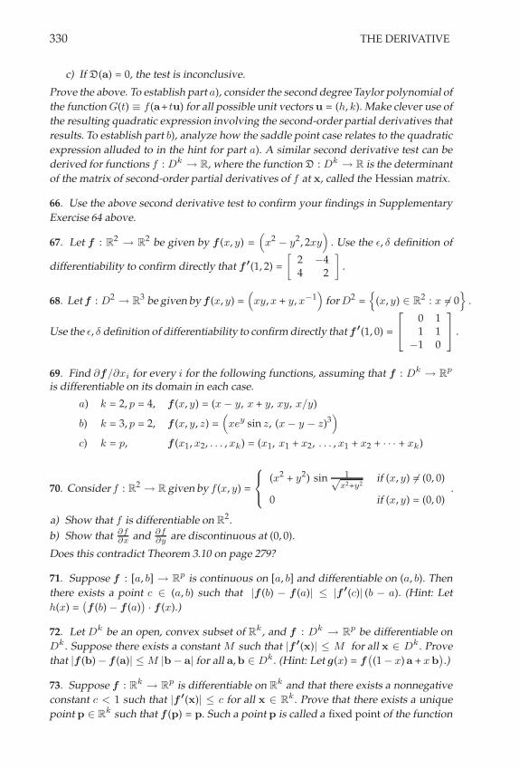
330 THE DERIVATIVE
c) If D(a) = 0, the test is inconclusive.
Prove the above. To establish part a), consider the second degree Taylor polynomial ofthe function G(t) . f (a+tu) for all possible unit vectors u = (h, k). Make clever use ofthe resulting quadratic expression involving the second-order partial derivatives thatresults. To establish part b), analyze how the saddle point case relates to the quadraticexpression alluded to in the hint for part a). A similar second derivative test can bederived for functions f : D
k , R, where the function D : Dk , R is the determinant
of the matrix of second-order partial derivatives of f at x, called the Hessian matrix.
66. Use the above second derivative test to confirm your findings in SupplementaryExercise 64 above.
67. Let f : R2 , R
2 be given by f (x, y) =(x
2 & y2, 2xy
). Use the $, . definition of
differentiability to confirm directly that f !(1, 2) =
92 &44 2
:.
68. Let f : D2 , R
3 be given by f (x, y) =(xy, x + y, x!1
)for D
2 =!
(x, y) " R2 : x %= 0
".
Use the $, . definition of differentiability to confirm directly that f !(1, 0) =
5
60 11 1
&1 0
7
8 .
69. Find (f/(xi for every i for the following functions, assuming that f : Dk , R
p
is differentiable on its domain in each case.
a) k = 2, p = 4, f (x, y) = (x & y, x + y, xy, x/y)
b) k = 3, p = 2, f (x, y, z) =(xe
y sin z, (x & y & z)3)
c) k = p, f (x1, x2, . . . , xk) = (x1, x1 + x2, . . . , x1 + x2 + · · · + xk)
70. Consider f : R2 , R given by f (x, y) =
RT
U(x2 + y
2) sin 1*x2+y2
if (x, y) %= (0, 0)
0 if (x, y) = (0, 0).
a) Show that f is differentiable on R2.
b) Show that (f
(xand (f
(yare discontinuous at (0, 0).
Does this contradict Theorem 3.10 on page 279?
71. Suppose f : [a, b] , Rp is continuous on [a, b] and differentiable on (a, b). Then
there exists a point c " (a, b) such that |f (b) & f (a)| # |f !(c)| (b & a). (Hint: Leth(x) =
,f (b) & f (a)
-· f (x).)
72. Let Dk be an open, convex subset of R
k , and f : Dk , R
p be differentiable onD
k . Suppose there exists a constant M such that |f !(x)| # M for all x " Dk . Prove
that |f (b) & f (a)| # M |b & a| for all a, b " Dk . (Hint: Let g(x) = f
,(1 & x) a + xb
-.)
73. Suppose f : Rk , R
p is differentiable on Rk and that there exists a nonnegative
constant c < 1 such that |f !(x)| # c for all x " Rk. Prove that there exists a unique
point p " Rk such that f (p) = p. Such a point p is called a fixed point of the function

SUPPLEMENTARY EXERCISES 331
f . Hints:1. Show that |f (x) & f (y)| # c |x & y| for all x, y " R
k .2. Let x0 be a point in R
k and define xn+1 = f (xn) for all n ' 1.Show that lim xn = p exists.
3. Show that f (p) = p.
74. Let D2 be an open disk in R
2, and f : D2 , R differentiable on D
2 such that(f
(x(x, y) = 0 for all (x, y) " D
2. Show that f (x, y) depends only on y.
75. Let D2 = R1 0 R2 0 R3, where R1 = (0, 1) + (0, 6), R2 = [1, 2] + (5, 6), and
R3 = (2, 3) + (0, 6). If f : D2 , R is differentiable on the interior of D
2 such that(f
(x(x, y) = 0 for all interior points (x, y) " D
2, does it follow that f (x, y) depends onlyon y?
76. Suppose f : R2 , R has the property that there exist two constants M1 and M2
such that for all (x, y) " R2,
&&&(f
(x(x, y)
&&& # M1 and&&&(f
(y(x, y)
&&& # M2. Show that f is
continuous on R2.
77. Suppose D2 is open in R
2 and that f : D2 , R is such that f and all mixed partial
derivatives of order # 3 are continuous on D2. Show that on D
2, fxxy = fxyx = fyxx.
78. Suppose f : R2 , R has continuous first- and second-order partial derivatives. If
gab(t) . f (at, bt) has a local minimum at t = 0 for every choice of real numbers a andb, does f have a local minimum at (0, 0)?
79. Consider the function f : R2 , R given by f (x, y) =
Ex
2y
x4+y2 for (x, y) %= (0, 0)
0 for (x, y) = (0, 0).
a) Is f continuous at (0, 0)?
b) Do the partial derivatives fx and fy exist at (0, 0)?
c) Is f differentiable at (0, 0)?
80. If f : R2 , R is given by f (x, y) =
E(x + y)2 sin(1/y) for (x, y) %= (0, 0)
0 for (x, y) = (0, 0), is fy
continuous at (0, 0)?
81. Suppose f : R2 , R has continuous partial derivatives up to order k ' 2, and for
all a, b " R the function ga,b : R , R given by ga,b(t) . f (at, bt) has a local minimumat t = 0. Show that f has a local minimum at (0, 0). (The order k may be chosen to beany value greater than or equal to 2 for convenience in justifying your answer.)
82. Consider the function f : C , C given by f (z) = 2z2 & 3. Use the $, . version of
the derivative to show that f#(1) %= 3. Hint: Use the method of proof by contradiction.

332 THE DERIVATIVE
83. In each of the following, consider the function f : D , C that is given, and findas large a domain D as is possible for the function f . Also find the correspondingdomain of f
#. a) f (z) = z5
b) f (z) = |z| c) f (z) = z2/3
84. Determine the values of z for which the following functions are differentiable(presume the natural domain for f in each case). First, use the Jacobian to infer whatthe derivative should be, and then use the Cauchy-Riemann equations to find thederivative in each case.a) f (z) = (z & 1)!1
b) f (z) = z3
c) f (z) = sinh z
d) f (z) = z2 + (z)2
e) f (z) = &2xy + i
(x
2 & y2)
f ) f (z) = 2xy + i x2
g) f (z) = ex + i e
yh) f (z) = x
3y & y
3x + i
(32 x
2y
2 & 14 y
4 & 14 x
4)
85. Suppose u : R2 , R is given by u(x, y) = xy. Can you find a (complex) differen-
tiable function f : C , C such that Re (f ) = u?
86. Suppose v : R2 , R is given by v(x, y) = x
2y. Can you find a (complex) differen-
tiable function f : D , C such that Im(f ) = v?
87. Suppose u : D2 , R is such that its second-order partial derivatives exist and are
continuous on D2, and #u . uxx+uyy = 0 on D
2. Such a function u is called harmonicon D
2. What would you need to assume in order to find a function f : D , C suchthat Re(f ) = u? What if you require f to be differentiable?
88. Suppose f : D , C given by f (z) = u(x, y) + i v(x, y) is differentiable on D ! C,and that the functions u and v satisfy the conditions of the mixed derivative theoremon page 267. Compute #u and #v. What can you conclude? We will see in a laterchapter that differentiablity of the complex function f implies these other conditionson its real and imaginary parts u and v, and so the conclusion you come to will applyto the real and imaginary parts of any differentiable complex function.
89. Compare your results from the last exercise to what you find for the real function
g : D2 , R
2 given by g(x, y) =(x
2 + y, x2 + y
2)
.
90. Suppose the function f : D , C is given in polar coordinates as f (z) = u(r, %) +
i v(r, %), and that f is defined in a neighborhood of the point z0 = r0ei %0 %= 0. Un-
der the right conditions (which?), show that the Cauchy-Riemann equations in polarcoordinates are given by
ur =1r
v% and1r
u% = &vr.
91. Show that the Laplacian operator # . (2
(x2 + (2
(y2 can be expressed in terms of (
(z
and (
(zas # = 4 (
(z
(
(z.
92. Suppose we have a function of two complex variables, f (z1, z2). Show that such afunction can be written in the form f (z1, z2) = F (z1, z1, z2, z2), where z1 = x1+i y1, z1 =x1 & i y1, z2 = x2 + i y2, and z2 = x2 & i y2.

SUPPLEMENTARY EXERCISES 333
93. Find F for the following functions.
a) f (z1, z2) = z21 + z1z2 b) f (z1, z2) = |z1|ez2 c) f (z1, z2) = Im(z1z2)
94. For the functions you found in the previous exercise, formally determine thefollowing: (F/(z1, (F/(z2, (F/(z1, and (F/(z2.
95. One could define f (z1, z2) to be differentiable if after finding its associated func-tion F (z1, z1, z2, z2) it was determined that (F/(z1 = (F/(z2 = 0. Which functions inthe previous exercise would be differentiable according to this definition?
96. Given the above definition of differentiability for functions of more than one com-plex variable, is there a corresponding set of “Cauchy-Riemann equations¿‘ Explorethis possibility.
97. Let f : R2 , R be given by f (x, y) = x
2 + y2 & 1. Use the implicit function
theorem to solve for y = g(x) in a neighborhood of ( 1"2
, 1"2
). Can this be done in a
neighborhood of (1, 0)?
98. Consider the equation x3 + y cos xy = 0. Can you solve for y = f (x) in a neighbor-
hood of (0, 0)? Can you solve for x = g(y) in a neighborhood of (0, 0)?
99. Consider the equation x2y & z ln x + e
z = 1. Can you solve for z = f (x, y) in aneighborhood of (1, 0, 0)? Can you solve for x = g(y, z) in a neighborhood of (1, 0, 0)?Can you solve for y = h(x, z) in a neighborhood of (1, 0, 0)?
100. Consider the system of equations given below and determine whether you cansolve for z in terms of x, y, and w:
x & y + z + w8 = 0
2x + y & z + w = 0
y + z & 3w = 0.


7REAL INTEGRATION
God does not care about our mathematical difficulties. He integrates empirically.
Albert Einstein
We begin by studying what will be defined as the Riemann integral of a func-tion f : [a, b] 3 R over a closed interval. Since the Riemann integral is theonly type of integral we will discuss in detail,1 any reference to the integral ofa function should be understood to be the Riemann integral of that function.One motivation for the development of the Riemann integral corresponds tothe special case where such a function f is continuous and nonnegative on itsdomain. We may then determine the area under the curve described by thegraph of f in the xy-plane lying above the x-axis. The key idea, so familiar toall students of calculus, is to approximate the area by a finite sum of rectangu-lar subareas, a so-called Riemann sum, and then take the appropriate limit toobtain the exact area under the curve, the value of which corresponds to thevalue of the integral in this case. Even this special case prompts some naturalquestions. What other kinds of functions will obtain a limit in this process?Must the associated Riemann sum be set up in a particular way? Of course,we will be able to define such a Riemann integral even when the function fis negative over part of, or even all of, its domain. However, in such cases weusually forgo the interpretation of the integral as an area, instead relying onthe more abstract notion of the integral as the limit of a Riemann sum.
1 THE INTEGRAL OF f : [a, b] 3 R
1.1 Definition of the Riemann Integral
We begin with the following definition.
1Other types include the Riemann-Stieltjes integral, the Lebesgue integral, the Lebesgue-Stieltjes integral, and the Daniell integral. Each was developed, in some measure, to amendperceived shortcomings of the integral type that preceded it historically.
335

336 REAL INTEGRATION
Definition 1.1 A partition of [a, b] ' R is an ordered collection of n+1 pointsP = {x0, x1, x2, . . . , xn} ' [a, b],
such that a = x0 < x1 < x2 < · · · < xn = b. Each partition P determines
a collection of n subintervals {Ij} of [a, b], each given by
Ij = [xj"1, xj] for 1 + j + n.
The length of each subinterval Ij is denoted by
#xj / xj " xj"1.
Finally, the norm of the partition P is the length of the largest subintervaldetermined by P , and is given by
2P2 / max1*j*n
#xj .
We now introduce the useful concept of a refinement of a partition P .
Definition 1.2 A refinement of a partition P on [a, b] is any partition P& on
[a, b] satisfyingP ' P
&.
A simple example that illustrates the above definition is to consider the in-terval [0, 1] and the partition P =
.0, 1
2 , 1/
. One refinement of P is P& =.
0, 14 , 1
2 , 34 , 1
/. The partition given by P
&& =.
0, 14 , 3
4 , 1/
is not a refinementof P . (Why?) Finally, we will sometimes have need to form the union of twopartitions, and we do this in a very natural way. For example, P1 = {0, 1
2 , 1}
and P2 = {0, 14 , 1
3 , 1} are partitions of [0, 1], and P3 = {1, 32 , 2} is a partition of
[1, 2]. The partition P = P1 % P2 / {0, 14 , 1
3 , 12 , 1} is also a partition of [0, 1],
and GP = P1 % P3 / {0, 1
2 , 1, 32 , 2} is a partition of [0, 2]. With the concept of a
partition of an interval established, we now define a Riemann sum associatedwith a function f : [a, b] 3 R.
Definition 1.3 Consider f : [a, b] 3 R and suppose P = {x0, x1, x2, . . . , xn}
is a partition of [a, b]. Let C = {c1, c2, . . . , cn} be a collection of points suchthat cj # Ij for 1 + j + n. Then the Riemann sum of f associated with thepartition P and the collection C is given by
SP (f , C) /n+
j=1
f (cj)#xj .
It is important to note that the value of the Riemann sum SP (f , C) describedin the above definition will, in general, depend on the partition P and thechoice of points C, as well as on the function f .

THE INTEGRAL OF f : [a, b] , R 337
Example 1.4 Let f : [0, 1] 3 R be given by f (x) = x2 +1, and let P =.
0, 13 , 1
/
be a partition of [0, 1]. The subintervals associated with P are I1 =A0, 1
3
Band
I2 =A
13 , 1
B, and the norm of P is 2P2 = 2
3 . Computing SP (f , C) for C =.
0, 12
/,
we obtainSP (f , C) = f (0) 1
3 + f(
12
)23 = 7
6 . "
! 7.1 Consider the function from the previous example.a) Using the same partition as given in the example, compute the Riemann
sum SP (f , C) associated with C =. 1
4 , 34
/.
b) Using the same C as in the example, compute the Riemann sum SP (f , C)
associated with the partition P =.
0, 18 , 1
/.
c) Compute the Riemann sum SP% (f , C#) associated with the refinement
P # =.
0, 18 , 1
3 , 1/
of the partition from the example, and C# =.
0, 18 , 1
3
/.
d) Compute the Riemann sums SPn (f , Cn) associated with the partitions
Pn =.
0, 1n
, 2n
, . . . , 1/
and associated Cn =. 1
n, 2
n, . . . , 1
/for n = 3, 5,
8, and 10. What seems to be happening here?
If f (x) ! 0 is continuous on [a, b], it is easy to see that SP (f , C) approxi-mates the area under the curve above the x-axis between a and b. For a fixedpartition P of [a, b] we may adjust C = {c1, . . . , cn} to obtain a better approx-imation to the area, but in general it is easier to improve the approximationby reducing 2P2. This can be accomplished through the use of a “finer“ par-tition, achieved by increasing n. Ultimately, and under suitable conditions,letting n 3 - forces 2P2 3 0, and the associated Riemann sum approachesthe exact area. This idea is summarized in the following definition, whichalso specifies what it means for a function f : [a, b] 3 R to be integrable on[a, b].
Definition 1.5 We say that
lim&P�
SP (f , C) = L
exists if and only if for each ! > 0 there exists . > 0 such that for any partitionP of [a, b] satisfying 2P2 < ., and for any corresponding choice of C, weobtain
|SP (f , C) " L| < !.
We say that f : [a, b] 3 R is integrable on [a, b] if and only if
lim&P�
SP (f , C) = L
exists. In this case we refer to L as the integral of f from a to b, and we writeY b
af (x) dx = L.

338 REAL INTEGRATION
Note that the above definition implies that when f : [a, b] 3 R is integrable
on [a, b], thenZ ba f (x) dx / lim&P� SP (f , C). Also note that when we refer
to the integral of a function “on [a, b],“ we are referring to the integral from ato b. Finally, it is worth mentioning that what we call an integrable functionas described by Definition 1.5 is more specifically called a Riemann integrablefunction in texts that treat other types of integrals. Since we will only developthe Riemann integral in what follows, we simply refer to such functions asintegrable.
To maintain consistency in our development, we define the following quan-tity for an integrable function f : [a, b] 3 R, namely,
Y a
bf (x) dx / "
Y b
af (x) dx. (7.1)
This effectively defines the integral of f from b to a in terms of the integralof f from a to b. Also note that for any integrable f : [a, b] 3 R, and anyc # [a, b], we define Y c
cf (x) dx / 0. (7.2)
The somewhat arbitrary nature of the identities (7.1) and (7.2) can be ex-plained through a more detailed development of the Riemann sum concept,which the reader may explore in the supplementary exercises section of thischapter.
Note that according to Definition 1.5, if f : [a, b] 3 R is integrable on [a, b],then for each ! > 0 there exists . > 0 such that for any partition P of [a, b]satisfying 2P2 < ., and any corresponding choice of C, we obtain
&&&&&SP (f , C) "
Y b
af (x) dx
&&&&& < !.
Therefore, for such an integrable f , we may choose a convenient sequence
of partitions, say, Pn = {a = x0, x1, . . . , xn = b} where xj = a + j (b"a)n for
0 + j + n, and associated points Cn = {c1, . . . , cn} with cj = xj # Ij for
1 + j + n, for which it follows that 2Pn2 = b"an and SPn (f , Cn) =
;nj=1 f
,a +
j (b"a)n
-(b"an
). Note that with such a choice, we have that 2Pn2 = b"a
n < .
as long as n >(
b"a+
), and so choosing N # N such that N >
(b"a+
)obtains
the result
n > N )
&&&&&SPn (f , Cn) "
Y b
af (x) dx
&&&&& < !,
or more succinctly,
limn('
(b"an
) n+
j=1
f(a + j (b"a)
n
)=
Y b
af (x) dx. (7.3)

THE INTEGRAL OF f : [a, b] , R 339
Such a convenient choice of partitions is common in practice when a functionis known to be integrable on the interval in question, allowing the integralto be expressed as the limit of a Riemann sum with the limit being takenas n 3 -. We now give our first, and simplest, example of a subclass ofintegrable functions on a closed and bounded interval.
Example 1.6 Let f : [a, b] 3 R be given by f (x) = k, where k # R is aconstant. If P is any partition of [a, b], then
SP (f , C) =+
j
k #xj = k (b " a),
for all choices of C. Hence,
Y b
ak dx = lim
&P�SP (f , C) = k (b " a),
and so any function f : [a, b] 3 R that is constant on [a, b] is integrable on[a, b]. "
In the remainder of this section we will determine other subclasses of in-tegrable functions that are especially convenient and common and that areeasier to identify than the more general class of integrable functions given byDefinition 1.5. Also, we will derive the important properties of integrals thatallow for easier manipulation of them in various settings, and we will seesome examples of functions that are not integrable. While the definition ofintegrability in terms of Riemann sums given by Definition 1.5 is relativelystraightforward and conveys the relevant ideas in an uncluttered way, it isnot always easily applied. To remedy this, we will now recast integrabilityin terms of what are commonly referred to as upper and lower Riemann sums.This will require us to restrict our focus to bounded functions f : [a, b] 3 R.
1.2 Upper and Lower Sums and Integrals
Upper and Lower Sums and Their Properties
For all that follows in this subsection, we will presume that f : [a, b] 3 R is abounded function. We begin with a definition.
Definition 1.7 Consider the bounded function f : [a, b] 3 R, and let P be apartition of [a, b] having associated subintervals {Ij}. Finally, let Mj / sup
Ij
f
and let mj / infIj
f . Then the upper sum associated with f on [a, b] is given by
SP (f ) /n+
j=1
Mj#xj ,

340 REAL INTEGRATION
and the lower sum associated with f on [a, b] is given by
SP (f ) /n+
j=1
mj#xj .
Note in the above that supIj
f / sup{f (x) : x # Ij}, and likewise infIj
f /
inf{f (x) : x # Ij}. We now give an example.
Example 1.8 Consider f : [0, 1] 3 R given by f (x) = x2 + 1, and let P =.0, 1
3 , 1/
be a partition of [0, 1]. Clearly f is bounded on [a, b] since f is con-tinuous there. We will find the associated upper and lower sums. Note thatI1 =
A0, 1
3
B, and so
M1 = supI1
f =(
13
)2+ 1 = 10
9 ,
while I2 =A
13 , 1
B, and so
M2 = supI2
f = 12 + 1 = 2.
Therefore, we have that
SP (f ) = 109
(13
)+ 2
,23
-= 46
27 .
In a similar fashion, we find that
m1 = infI1
f = 02 + 1 = 1, and m2 = infI2
f =(
13
)2+ 1 = 10
9 .
Therefore, we have that
SP (f ) = 1(
13
)+ 10
9
,23
-= 29
27 . "
! 7.2 In what follows, let f : [a, b] , R be bounded.a) Suppose f : [a, b] , R is bounded, and that P = {a = x0, x1, . . . , xn = b} is a
partition of [a, b]. Fix any 0 < j < n, and let P1 = {a = x0, . . . , xj} and P2 ={xj , . . . , xn = b}, so that P = P1 0P2. Show that SP1)P2 (f ) = SP1
(f ) +SP2 (f ), andthat SP1)P2
(f ) = SP1(f ) + SP2
(f ).
b) Consider any bounded function f : [a, b] , R and suppose c " (a, b). If P1 = {a =x0, x1, . . . , xm = c} partitions [a, c] and P2 = {c = xm, . . . , xm+n = b} partitions[c, b], then P = P1 0 P2 is a partition of [a, b]. Show that SP1)P2 (f ) = SP1
(f ) +SP2 (f ), and that SP1)P2
(f ) = SP1(f ) + SP2
(f ).
Recall that in Example 1.4 on page 337 the value obtained for the Riemannsum associated with the same function and partition as in the above exam-ple was 7
6 , a value lying between the lower and upper sum values of 2927 and
4627 , respectively. This illustrates a general fact, and we state the result in thefollowing lemma.

THE INTEGRAL OF f : [a, b] , R 341
Lemma 1.9 For any bounded function f : [a, b] 3 R, any partition P of [a, b],and any associated choice of points C = {c1, . . . , cn},
SP (f ) + SP (f , C) + SP (f ).
! 7.3 Prove the above lemma.
Note that the above lemma also establishes that for any partition P , the lowersum associated with f is less than or equal to the upper sum associated withf , i.e.,
SP (f ) + SP (f ).
The above lemma will also enable us to study the integrability of boundedfunctions in terms of upper and lower sums, which are often easier to workwith than Riemann sums. In particular, we will ultimately show that the inte-gral of a bounded function f exists as described in Definition 1.5 on page 337if and only if the supremum of the associated lower sums equals the infimumof the associated upper sums. Before formally stating and proving this result,however, we will prove a series of lemmas establishing various properties ofupper and lower sums.
Lemma 1.10 Suppose f : [a, b] 3 R is a bounded function and P is a partition of[a, b]. If P & is a refinement of P , then
SP (f ) + SP !(f ) and SP !(f ) + SP (f ).
The lemma says that under refinements of a given partition, lower sumsnever decrease, and upper sums never increase.
PROOF We prove that SP ! (f ) + SP (f ) and leave the proof that SP (f ) +
SP ! (f ) to the reader. Note that it is only necessary to consider a “one point“refinement, since the general case can then be done by induction. To this end,suppose P = {x0, x1, . . . , xn} and P
& = P % {)}, where xk"1 < ) < xk forsome 1 + k + n. Then,
SP (f ) =n+
j=1
Mj#xj = M1#x1 + M2#x2 + · · · + Mn#xn,
and
SP !(f ) = M1#x1 + · · · + Mk"1#xk"1 + M leftk () " xk"1) + M
rightk (xk " ))
+Mk+1#xk+1 + · · · + Mn#xn,
whereM left
k / sup[xk"1, !]
f and Mrightk / sup
[!, xk]f .
Therefore,
SP (f ) " SP !(f ) = Mk#xk "
(M left
k () " xk"1) + Mrightk (xk " ))
). (7.4)

342 REAL INTEGRATION
To complete the proof, we note that
M leftk = sup
[xk"1,!]f + sup
Ik
f = Mk, and similarly, Mrightk + Mk.
This combined with (7.4) above yields
SP (f ) " SP ! (f ) ! Mk#xk "
(Mk() " xk"1) + Mk(xk " ))
)
= Mk#xk " Mk#xk
= 0.
That is,SP !(f ) + SP (f ). #
! 7.4 Complete the proof of the above lemma by showing that SP (f ) # SP% (f ).
The following lemma differs from the previous one in that it considers twopossibly different partitions of [a, b]. Basically, it says that lower sums arenever greater than upper sums.
Lemma 1.11 Suppose f : [a, b] 3 R is a bounded function, and P1 and P2 aretwo partitions of [a, b]. Then,
SP1(f ) + SP2
(f ).
PROOF Let P = P1 % P2. Then P is a refinement of P1 and of P2. By Lem-mas 1.9 and 1.10 on page 341, we have that
SP1(f ) + SP1.P2
(f ) + SP1.P2(f ) + SP2
(f ). #
Upper and Lower Integrals and Their Properties
For a given bounded function f : [a, b] 3 R, since every lower sum is lessthan or equal to every upper sum, and Riemann sums are caught betweenthem, it is reasonable to consider the supremum of the lower sums and theinfimum of the upper sums. If these values are the same, the common valuewill be shown to equal the limit of the Riemann sums, and hence the integralof f over [a, b]. In fact, for m + f + M on [a, b], it is easy to see that lowersums are bounded above, since
SP (f ) + SP (f ) =n+
j=1
Mj#xj +
n+
j=1
M #xj = M (b " a).
Therefore, the supremum of the lower sums exists. Similarly, one can showthat upper sums are bounded below, and hence, that the infimum of the up-per sums exists.
! 7.5 Show that, for a bounded function f : [a, b] , R, the upper sums are boundedbelow.

THE INTEGRAL OF f : [a, b] , R 343
With the above facts in mind, we make the following definition.
Definition 1.12 For any bounded function f : [a, b] 3 R, we define thelower integral of f over [a, b] by
Y b
af (x) dx / sup
PSP (f ).
Similarly, we define the upper integral of f over [a, b] by
Y b
af (x) dx / inf
PSP (f ).
Note in the above that
supP
SP (f ) / sup.SP (f ) : P is a partition of [a, b]
/.
Similarly,infP
SP (f ) / inf.SP (f ) : P is a partition of [a, b]
/.
As expected, the upper integral of a bounded function is never less than thelower integral of the function.
Theorem 1.13 Suppose f : [a, b] 3 R is a bounded function. Then,
Y b
af (x) dx +
Y b
af (x) dx.
PROOF Fix a partition P1 of [a, b], and note that for any other partition P of[a, b] we have
SP1(f ) + SP (f ).
Therefore,
SP1(f ) +
Y b
af (x) dx. (Why?)
Since P1 was arbitrary, it follows that SP (f ) +Z ba f (x) dx for all partitions P
of [a, b]. This yields Y b
af (x) dx +
Y b
af (x) dx,
and the theorem is proved. #
! 7.6 Suppose f , g : [a, b] , R are both bounded functions such that f (x) # g(x) on
[a, b]. Prove thatZ
b
af (x) dx #
Zb
ag(x) dx, and
Zb
af (x) dx #
Zb
ag(x) dx.
The following lemmas will be useful to us later.

344 REAL INTEGRATION
Lemma 1.14 Suppose f : [a, b] 3 R is a bounded function. Then, for any ! > 0there exists . > 0 such that if P is a partition of [a, b],
2P2 < . ) SP (f ) <
Y b
af (x) dx + ! and SP (f ) >
Y b
af (x) dx " !.
PROOF We establish the inequality SP (f ) <Z ba f (x) dx + ! and leave the in-
equality involving the lower sum to the reader. For ! > 0 we may choose apartition P1 of [a, b] such that
SP1(f ) <
Y b
af (x) dx + (
2 .
Now suppose P is a partition of [a, b] such that 2P2 < ., where . > 0 is to be
determined so that SP (f ) <Z ba f (x) dx+!. IfP2 = P%P1, then SP2
(f ) + SP1(f )
so that
SP (f ) =,SP (f ) " SP2
(f )-
+ SP2(f )
+
,SP (f ) " SP2
(f )-
+ SP1(f )
<,SP (f ) " SP2
(f )-
+
Y b
af (x) dx + (
2 . (7.5)
If we can show that,SP (f ) " SP2
(f )-
< (2 , we are done. To this end, we
describe the partitions P , P1, and P2 more explicitly by
P1 = {x&0, x&1, . . . , x&n},
P = {x0, x1, . . . , xm},
P2 = {x&&0 , x&&1 , . . . , x&&r},
and illustrate these partitions in Figure 7.1. Let .1 / minP1
(#x&j), and assume
that 2P2 < . < .1 so that every subinterval associated with P2 = P % P1is smaller than the smallest subinterval associated with P1, i.e., between anytwo points in P there is at most one point of P1. Then, denoting
Mj / sup[xj"1, xj]
f , and M &&j / sup0
x!!j"1, x!!
j
1f ,
we haveSP (f ) " SP2
(f ) =+
Mj#xj "
+M &&
j #x&&j . (7.6)
Note that for any subinterval that is common to P and P2 there is no con-tribution to SP (f ) " SP2
(f ). The only contributions come from subinter-vals Ij = [xj"1, xj] of P that have been subdivided by a point x&k from P1,i.e., Ij = [xj"1, xj ] = [xj"1, x&k] % [x&k , xj], where #xleft
j / x&k " xj"1, and
#xright
j / xj " x&k . Recall that #xj = xj " xj"1. There are no more than n such

THE INTEGRAL OF f : [a, b] , R 345
P1
P2
P
{x"
j}
{x""
j }
{xj}
Figure 7.1 The partitions P1,P , and P2.
subintervals from P , and each such subdivided subinterval Ij gives rise to acontribution to the right-hand side of (7.6) of the form
Ej =
2sup
[xj"1, xj ]f
3#xj "
5
62
sup[xj"1, x!
k]
f
3#xleft
j +
2sup
[x!k, xj ]
f
3#x
right
j
7
8 .
If we let " / sup[a, b]
|f |, then we have
|Ej | + 3 " 2P2 < 3 " ..
All of this yieldsSP (f ) " SP2
(f ) =&&SP (f ) " SP2
(f )&&
+ 3 " . n
< (2 ,
provided that . < (6 " n . Combining this with (7.5) obtains
SP (f ) <
Y b
af (x) dx + !,
provided that 2P2 < . / min,.1, (
6 " n
-. #
! 7.7 Complete the above proof by writing up the similar argument for the lowerintegral. What . must ultimately be used to establish the overall result?
Lemma 1.15 Suppose f : [a, b] 3 R is bounded on [a, b], and a < c < b. ThenY b
af (x) dx =
Y c
af (x) dx +
Y b
cf (x) dx,
and Y b
af (x) dx =
Y c
af (x) dx +
Y b
cf (x) dx.

346 REAL INTEGRATION
PROOF We will establish the equality for upper integrals. To this end, let Pbe a partition of [a, b]. Then P % {c} = P1 %P2 where P1 is a partition of [a, c],and P2 is a partition of [c, b]. Now, since
SP (f ) ! SP.{c}(f )
= SP1(f ) + SP2
(f ) by Exercise 7.2 on page 340,
!
Y c
af (x) dx +
Y b
cf (x) dx,
it follows that Y b
af (x) dx !
Y c
af (x) dx +
Y b
cf (x) dx. (7.7)
We now establish the reverse inequality. To this end, for any ! > 0 there existsa partition P1 of [a, c], and a partition P2 of [c, b] such that
SP1(f ) <
Y c
af (x) dx + (
2 , and SP2(f ) <
Y b
cf (x) dx + (
2 . (Why?)
Now, since P1 % P2 is a partition of [a, b], we have
Y b
af (x) dx + SP1.P2
(f )
= SP1(f ) + SP2
(f ) by Exercise 7.2 on page 340,
<
Y c
af (x) dx +
Y b
cf (x) dx + !.
This is true for every ! > 0, and therefore
Y b
af (x) dx +
Y c
af (x) dx +
Y b
cf (x) dx. (7.8)
Inequalities (7.7) and (7.8) together obtain
Y b
af (x) dx =
Y c
af (x) dx +
Y b
cf (x) dx.
We leave the proof of the lower integral equality to the reader. #
! 7.8 Answer the (Why?) question in the above proof, and prove the lower integralresult.
1.3 Relating Upper and Lower Integrals to Integrals
The following theorem is the key result of this section. It provides a meansfor determining the integrability of a function f : [a, b] 3 R, and its valuewhen it is integrable, via upper and lower integrals.

THE INTEGRAL OF f : [a, b] , R 347
Theorem 1.16 Suppose f : [a, b] 3 R is a bounded function. Then,
f : [a, b] 3 R is integrable if and only if
Y b
af (x) dx =
Y b
af (x) dx,
and in either case,Y b
af (x) dx =
Y b
af (x) dx =
Y b
af (x) dx.
PROOF SupposeZ ba f (x) dx =
Z ba f (x) dx. We will show that this implies that
f is integrable. To this end, consider ! > 0. By Lemma 1.14, there exists . > 0such that if P is a partition of [a, b],
2P2 < . ) SP (f ) <
Y b
af (x) dx + ! and SP (f ) >
Y b
af (x) dx " !.
From this we obtain, for 2P2 < . and any C associated with P ,
Y b
af (x) dx " ! < SP (f ) + SP (f , C) + SP (f ) <
Y b
af (x) dx + !. (7.9)
Denoting the common value ofZ ba f (x) dx and
Z ba f (x) dx by L, we obtain from
expression (7.9) that2P2 < . ) |SP (f , C) " L| < !,
i.e., lim&P�
SP (f , C) = L, (7.10)
and hence f is integrable on [a, b]. Note also that equality (7.10) establishes
thatZ ba f (x) dx =
Z ba f (x) dx =
Z ba f (x) dx. Now assume that f is integrable on
[a, b], i.e., lim&P�
SP (f , C) =Z ba f (x) dx exists. Then, for ! > 0 there exists . > 0
such that if P is a partition of [a, b],
2P2 < . )
&&&&&SP (f , C) "
Y b
af (x) dx
&&&&& <!
2.
Choose a partition P of [a, b] such that 2P2 < ., and select cj # Ij such thatfor Mj / sup
Ij
f ,
f (cj) > Mj "!
2 (b " a)for j = 1, . . . , n.
Then for C = {c1, . . . , cn},
SP (f , C) > SP (f ) " (2 !
Y b
af (x) dx "
(2 .

348 REAL INTEGRATION
Since SP (f , C) <Z ba f (x) dx + (
2 , it follows thatZ ba f (x) dx <
Z ba f (x) dx + ! for
all ! > 0. Hence, Y b
af (x) dx +
Y b
af (x) dx. (7.11)
If we choose cj # Ij such that, for mj / infIj
f ,
f (cj) < mj +!
2 (b " a),
we may similarly conclude thatY b
af (x) dx +
Y b
af (x) dx. (7.12)
Combining inequalities (7.11) and (7.12), we have
Y b
af (x) dx +
Y b
af (x) dx +
Y b
af (x) dx,
which impliesY b
af (x) dx =
Y b
af (x) dx =
Y b
af (x) dx.
#
Example 1.17 Consider the bounded function f : [0, 2] 3 R given by
f (x) =
E0 if 0 + x + 1
1 if 1 < x + 2.
We will show that f is integrable on [0, 2], and determine the value of the in-tegral. To this end, let P = {x0, x1, . . . , xn} be a partition of [0, 2]. We considertwo cases: Case 1 with xm"1 < 1 < xm, and case 2 with xm = 1. Note that incase 1,
SP (f ) =n+
j=m
#xj = xn " xm"1 = 2 " xm"1,
andSP (f ) =
n+
j=m+1
#xj = xn " xm = 2 " xm.
In case 2 we similarly have
SP (f ) = 1, and SP (f ) = 2 " xm+1.
We leave it to the reader to show that
infP
SP (f ) =
Y 2
0f (x) dx = 1, and sup
PSP (f ) =
Y 2
0f (x) dx = 1,
and therefore that f is integrable on [0, 2] andZ 2
0 f (x) dx = 1. "
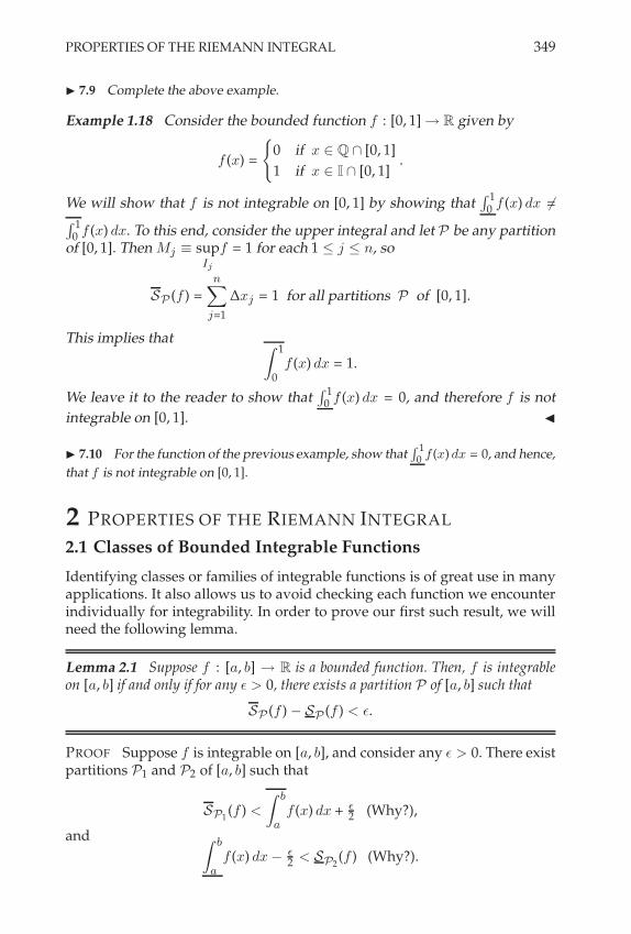
PROPERTIES OF THE RIEMANN INTEGRAL 349
! 7.9 Complete the above example.
Example 1.18 Consider the bounded function f : [0, 1] 3 R given by
f (x) =
E0 if x # Q & [0, 1]
1 if x # I & [0, 1].
We will show that f is not integrable on [0, 1] by showing thatZ 1
0 f (x) dx $=Z 1
0 f (x) dx. To this end, consider the upper integral and let P be any partitionof [0, 1]. Then Mj / sup
Ij
f = 1 for each 1 + j + n, so
SP (f ) =n+
j=1
#xj = 1 for all partitions P of [0, 1].
This implies that Y 1
0f (x) dx = 1.
We leave it to the reader to show thatZ 1
0 f (x) dx = 0, and therefore f is not
integrable on [0, 1]. "
! 7.10 For the function of the previous example, show thatZ 1
0 f (x) dx = 0, and hence,
that f is not integrable on [0, 1].
2 PROPERTIES OF THE RIEMANN INTEGRAL
2.1 Classes of Bounded Integrable Functions
Identifying classes or families of integrable functions is of great use in manyapplications. It also allows us to avoid checking each function we encounterindividually for integrability. In order to prove our first such result, we willneed the following lemma.
Lemma 2.1 Suppose f : [a, b] 3 R is a bounded function. Then, f is integrableon [a, b] if and only if for any ! > 0, there exists a partition P of [a, b] such that
SP (f ) " SP (f ) < !.
PROOF Suppose f is integrable on [a, b], and consider any ! > 0. There existpartitions P1 and P2 of [a, b] such that
SP1(f ) <
Y b
af (x) dx + (
2 (Why?),
and Y b
af (x) dx "
(2 < SP2
(f ) (Why?).

350 REAL INTEGRATION
Now let P = P1 % P2. Then,
SP (f ) + SP1(f ) <
Y b
af (x) dx + (
2 =
Y b
af (x) dx + (
2 ,
andSP (f ) ! SP2
(f ) >
Y b
af (x) dx "
(2 =
Y b
af (x) dx "
(2 ,
which together implySP (f ) " SP (f ) < !.
Now suppose that for any ! > 0 there exists a partition P of [a, b] such thatSP (f ) " SP (f ) < !. To prove that f is integrable on [a, b], note that
0 +
Y b
af (x) dx "
Y b
af (x) dx + SP (f ) " SP (f ) < !.
Since this is true for every ! > 0, it follows thatZ ba f (x) dx =
Z ba f (x) dx, and
the lemma is proved. #
! 7.11 Answer the two (Why?) questions in the above proof.
The following important example makes critical use of the above lemma.
Example 2.2 Suppose the bounded function f : [a, b] 3 R is nonnegativeand integrable on [a, b]. The reader can easily verify that
,
f is then boundedon [a, b]. We will show that
,
f is also integrable on [a, b]. To this end, consider. > 0 and let P be a partition of [a, b] such that
SP (f ) " SP (f ) < .2. (7.13)
Note that for Mj / supIj
f and mj / infIj
f ,
SP,%
f-" SP
,%f-
=n+
j=1
(*Mj "
,mj
)#xj . (7.14)
We now split up the sum in (7.14) according to
A / {j : Mj " mj < .} and B / {j : Mj " mj ! .}.
That is,
SP,%
f-" SP
,%f-
=+
j#A
(*Mj "
,mj
)#xj +
+
j#B
(*Mj "
,mj
)#xj .
(7.15)Note that
j # A )
*Mj "
,mj +
*Mj " mj <
,
., (Why?)
and therefore +
j#A
(*Mj "
,mj
)#xj <
,
. (b " a). (7.16)

PROPERTIES OF THE RIEMANN INTEGRAL 351
Also note that inequality (7.13) yields
.2 > SP (f ) " SP (f ) =n+
j=1
(Mj " mj) #xj
!
+
j#B
(Mj " mj) #xj
! .+
j#B
#xj ,
and so +
j#B
#xj + .. (7.17)
Inequality (7.17) now yields that+
j#B
(*Mj "
,mj
)#xj +
,
M+
j#B
#xj +
,
M ., (7.18)
where M / sup[a, b]
f . Finally, we have that
SP,%
f-" SP
,%f-
=+
j#A
(*Mj "
,mj
)#xj +
+
j#B
(*Mj "
,mj
)#xj
<,
. (b " a) +,
M . by (7.16) and (7.18),
< ! if . < min
$(
2($
M+1) ,
0(
2 (b"a)
124
.
Therefore,,
f is integrable on [a, b]. "
! 7.12 Verify that*
f is bounded on [a, b], and answer the (Why?) question in theabove example.
Using Lemma 2.1, we can now prove that continuous functions on [a, b] areintegrable on [a, b].
Theorem 2.3 If f : [a, b] 3 R is continuous on [a, b], then f is integrable on[a, b].
PROOF Since f is continuous on the closed interval [a, b], it is also boundedthere. Consider any ! > 0. We will find a partition P of [a, b] such that SP (f )"SP (f ) < !. To this end, note that since f is continuous on the compact set[a, b], it is uniformly continuous there. Therefore, there exists . > 0 such thatfor ), , # [a, b],
|) " ,| < . ) |f ()) " f (,)| <!
(b " a).
Now choose partition P of [a, b] such that 2P2 < ., and consider
SP (f ) " SP (f ) =n+
j=1
,Mj " mj
-#xj . (7.19)
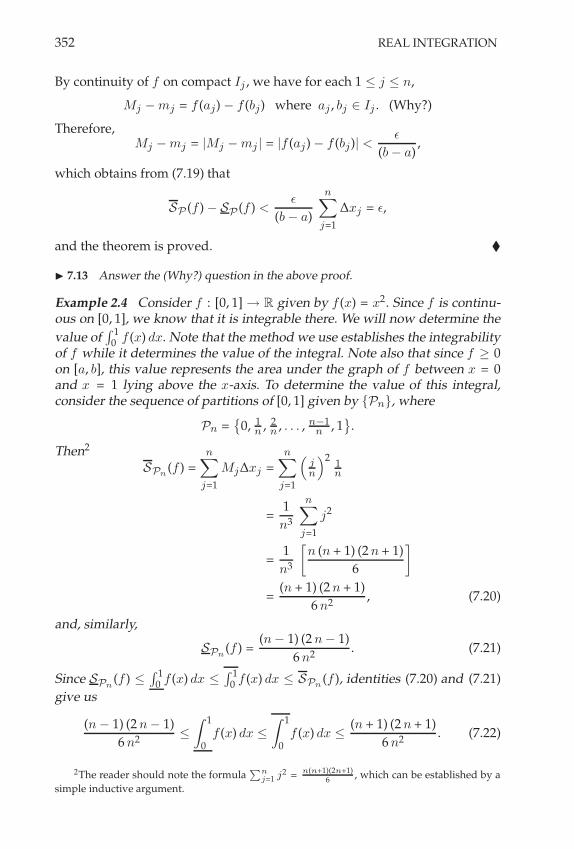
352 REAL INTEGRATION
By continuity of f on compact Ij , we have for each 1 + j + n,
Mj " mj = f (aj) " f (bj) where aj , bj # Ij . (Why?)
Therefore,Mj " mj = |Mj " mj | = |f (aj) " f (bj)| <
!
(b " a),
which obtains from (7.19) that
SP (f ) " SP (f ) <!
(b " a)
n+
j=1
#xj = !,
and the theorem is proved. #
! 7.13 Answer the (Why?) question in the above proof.
Example 2.4 Consider f : [0, 1] 3 R given by f (x) = x2. Since f is continu-ous on [0, 1], we know that it is integrable there. We will now determine the
value ofZ 1
0 f (x) dx. Note that the method we use establishes the integrabilityof f while it determines the value of the integral. Note also that since f ! 0on [a, b], this value represents the area under the graph of f between x = 0and x = 1 lying above the x-axis. To determine the value of this integral,consider the sequence of partitions of [0, 1] given by {Pn}, where
Pn =.
0, 1n , 2
n , . . . , n"1n , 1
/.
Then2
SPn (f ) =n+
j=1
Mj#xj =n+
j=1
(jn
)21n
=1
n3
n+
j=1
j2
=1
n3
9n (n + 1) (2 n + 1)
6
:
=(n + 1) (2 n + 1)
6 n2, (7.20)
and, similarly,
SPn(f ) =
(n" 1) (2 n" 1)
6 n2. (7.21)
Since SPn(f ) +
Z 10 f (x) dx +
Z 10 f (x) dx + SPn (f ), identities (7.20) and (7.21)
give us
(n " 1) (2 n" 1)
6 n2+
Y 1
0f (x) dx +
Y 1
0f (x) dx +
(n + 1) (2 n + 1)
6 n2. (7.22)
2The reader should note the formula;n
j=1 j2 = n(n+1)(2n+1)6 , which can be established by a
simple inductive argument.

PROPERTIES OF THE RIEMANN INTEGRAL 353
Letting n 3 - in (7.22) then yields
1
3+
Y 1
0f (x) dx +
Y 1
0f (x) dx +
1
3,
and thereforeY 1
0f (x) dx =
Y 1
0f (x) dx =
Y 1
0f (x) dx =
1
3.
"
! 7.14 Consider f : [0, 1] , R given by f (x) = x. Is f integrable on [0, 1]? FindZ 1
0 f (x) dx andZ 1
0 f (x) dx, and show they are equal. From this, determineZ 1
0 f (x) dx.
Do the same for g : [0, 1] , R given by g(x) = x3. You will need the formula
;n
j=1 j3 =
n2 (n+1)2
4 .
The following theorem establishes another important class of integrable boundedfunctions.
Theorem 2.5 If f : [a, b] 3 R is bounded and monotone on [a, b], then f isintegrable on [a, b].
PROOF We consider the case where f is nondecreasing, and leave the non-increasing case to the reader. If f (a) = f (b) we are done (Why?), so supposef (a) < f (b). Consider any ! > 0, and choose a partition P of [a, b] such that2P2 < (
f (b)"f (a) . Then
SP (f ) " SP (f ) =n+
j=1
(Mj " mj) #xj
=n+
j=1
,f (xj) " f (xj"1)
-#xj
<!
f (b) " f (a)
n+
j=1
,f (xj ) " f (xj"1)
-
=!
f (b) " f (a)(f (b) " f (a))
= !,
and the theorem is proved in the nondecreasing case. #
! 7.15 Answer the (Why?) in the above proof, and finish the proof by handling thecase where f is nonincreasing.
The following theorem establishes yet another important class of integrablebounded functions.

354 REAL INTEGRATION
Theorem 2.6 If f : [a, b] 3 R is bounded and has finitely many discontinuitieson [a, b], then f is integrable on [a, b].
PROOF We consider the case where f has exactly one discontinuity on [a, b],and we assume it is also in (a, b). In particular, we leave the case of this dis-continuity being at one of the endpoints, and the more general case of f hav-ing more than one discontinuity, to the reader. To this end, let x0 # (a, b) bethe only discontinuity of f on [a, b], and consider any ! > 0. We will ap-ply Lemma 2.1 on page 349. For " / sup
[a,b]
|f (x)|, choose . > 0 such that
(x0"., x0 +.) ' (a, b). Then f is integrable on each of [a, x0".] and [x0 +., b],since f is continuous on each of these intervals. Therefore, there exists a par-tition P1 of [a, x0 " .] such that
SP1(f ) " SP1
(f ) < (3 ,
and there exists a partition P2 of [x0 + ., b] such that
SP2(f ) " SP2
(f ) < (3 .
Now, P = P1 % P2 is a partition of all of [a, b], and
SP (f ) " SP (f ) = SP1(f ) " SP1
(f ) + (2 .)(
sup[x0"", x0+"]
f)
" (2 .)(
inf[x0"", x0+"]
f)
+ SP2(f ) " SP2
(f )
< (3 + 4 . " + (
3 .
Choose . < (12 "
to obtain the result. #
! 7.16 Prove the case with x0 = a or x0 = b, as well as the case of more than onediscontinuity in the above theorem. What can happen if there are infinitely manydiscontinuities in [a, b]?
2.2 Elementary Properties of Integrals
We now prove several convenient and familiar properties of integrals of boundedfunctions.
Algebraic Properties
The following theorem establishes two properties that together are often re-ferred to as the linearity property of the integral.
Theorem 2.7 Suppose f : [a, b] 3 R and g : [a, b] 3 R are both bounded andintegrable on [a, b]. Then

PROPERTIES OF THE RIEMANN INTEGRAL 355
a) kf : [a, b] 3 R is bounded and integrable on [a, b] for all k # R, andY b
ak f (x) dx = k
Y b
af (x) dx.
b) f ± g : [a, b] 3 R is bounded and integrable on [a, b], andY b
a(f ± g)(x) dx =
Y b
af (x) dx ±
Y b
ag(x) dx.
PROOF We leave it to the reader to verify that kf and f ± g are boundedon [a, b]. To prove integrability in part a), let P be any partition of [a, b] withassociated C. Then,
SP (k f , C) =n+
j=1
k f (cj) #xj = k SP (f , C).
Since f is integrable on [a, b], for any ! > 0 there exists . > 0 such that
2P2 < . )
&&&&SP (f , C) "
Y b
af (x) dx
&&&& <!
|k| + 1.
Therefore, 2P2 < . implies&&&&SP (kf , C) " k
Y b
af (x) dx
&&&& =
&&&&k SP (f , C) " k
Y b
af (x) dx
&&&&
= |k|
&&&&SP (f , C) "
Y b
af (x) dx
&&&&
< |k|
2!
|k| + 1
3< !.
That is, Y b
ak f (x) dx = lim
&P�SP (k f , C) = k
Y b
af (x) dx.
To prove integrability in part b), let P be any partition of [a, b]. Then,
SP (f ± g, C) =n+
j=1
,f (cj) ± g(cj)
-#xj = SP (f , C) ± SP (g, C).
It is left to the reader to show that
lim&P�
SP (f ± g, C) = lim&P�
SP (f , C) ± lim&P�
SP (g, C),
and hence, Y b
a(f ± g)(x) dx =
Y b
af (x) dx ±
Y b
af (x) dx.
#
! 7.17 Complete the proof of part a) by showing that kf is bounded on [a, b] andthat lim
&P�SP (k f , C) = k lim
&P�SP (f , C).

356 REAL INTEGRATION
! 7.18 Complete the proof of part b) by showing that f ± g is bounded on [a, b] andthat lim
&P�SP (f ± g, C) = lim
&P�SP (f , C) ± lim
&P�SP (g, C).
We would next like to prove that if two functions are bounded and integrableover a closed interval, their product is also bounded and integrable over thatinterval. To do so we will need the following two technical lemmas.
Lemma 2.8 Suppose f : [a, b] 3 R is bounded and integrable on [a, b]. Thenf+ : [a, b] 3 R given by
f+(x) =
E0 when f (x) < 0
f (x) when f (x) ! 0,
and f" : [a, b] 3 R given by
f"(x) =
E"f (x) when f (x) < 0
0 when f (x) ! 0,
are also bounded and integrable on [a, b].
PROOF We consider the case of f+, and leave the f" case to the reader.Clearly f+ is bounded on [a, b]. Let P be a partition of [a, b] and define M+
j /
supIj
f+ and m+j / inf
Ij
f+. Then M+j " m+
j + Mj " mj (Why?). Therefore, for
! > 0 there exists a partition P of [a, b] such that
SP (f+) " SP (f+) + SP (f ) " SP (f ) < !.
This establishes the integrability of f+ on [a, b]. #
! 7.19 Answer the (Why?) question in the above proof, and prove the case for f!.
Lemma 2.9 Suppose f : [a, b] 3 R and g : [a, b] 3 R are both bounded, nonneg-ative and integrable on [a, b]. Then fg : [a, b] 3 R is also bounded and integrableon [a, b].
PROOF We leave it to the reader to verify that fg is bounded on [a, b]. Let P
be a partition of [a, b] and define Mfgj / sup
Ij
(fg) and mfgj / inf
Ij
(fg). Then,
since
Mfgj + M
fj M
gj and m
fgj ! m
fj m
gj , (Why?)

PROPERTIES OF THE RIEMANN INTEGRAL 357
we have that
SP (fg) " SP (fg) =+
j
,M
fgj " m
fgj
-#xj
+
+
j
,M
fj M
gj " m
fj m
gj
-#xj
=+
j
0M
fj
,M
gj " m
gj
-+ m
gj
,M
fj " m
fj
-1#xj
+ Mf,SP (g) " SP (g)
-+ Mg
,SP (f ) " SP (f )
-, (7.23)
where Mf = sup[a,b]
f and Mg = sup[a,b]
g. Now, since f and g are integrable on
[a, b], there exists a partition P of [a, b] such that
SP (g) " SP (g) <!
2 (Mf + 1), and SP (f ) " SP (f ) <
!
2 (Mg + 1),
which together with (7.23) imply
SP (fg) " SP (fg) < !,
and the result is proved. #
! 7.20 Verify that fg is bounded on [a, b], and answer the (Why?) question in the
above proof. In particular, show that Mfg
j# M
f
jM
g
j, and that m
fg
j' m
f
jm
g
j.
We can now state the following more general result, the proof of which is leftto the reader.
Theorem 2.10 Suppose f : [a, b] 3 R and g : [a, b] 3 R are both bounded andintegrable on [a, b]. Then fg : [a, b] 3 R is also bounded and integrable on [a, b].
! 7.21 Prove the above theorem, noting that f (x) = f+(x)&f
!(x), and g(x) = g+(x)&
g!(x).
Theorem 2.11 Suppose f : [a, b] 3 R and g : [a, b] 3 R are both bounded andintegrable on [a, b].
a) If f (x) + g(x) on [a, b], thenZ ba f (x) dx +
Z ba g(x) dx.
b) |f (x)| is integrable on [a, b], and&&&Z ba f (x) dx
&&& +Z ba |f (x)| dx.
PROOF To prove a), define h : [a, b] 3 R by h(x) = g(x)" f (x), and note thath(x) ! 0 on [a, b] and that h is integrable according to part b) of Theorem 2.7on page 354. Also, for any partition P of [a, b] we have
SP (h, C) =n+
j=1
h(cj) #xj ! 0.

358 REAL INTEGRATION
It is left to the reader to show that lim&P�
SP (h, C) ! 0, and therefore,
Y b
ah(x) dx ! 0.
Again by part b) of Theorem 2.7, we then haveY b
af (x) dx +
Y b
ag(x) dx.
To establish part b) of the present theorem, we note that if f is integrable thenf+ and f" are integrable. Since |f | = f+ + f", it follows that |f | is integrable.The details of the rest of the proof of part b) are left to the reader. #
! 7.22 Complete the proof of part a) by considering the bounded function h : [a, b] ,R satisfying h(x) ' 0 on [a, b]. Show that lim
&P�SP (h, C) ' 0. Complete the proof of
part b).
The following corollary to the above theorem is a useful result on its own.
Corollary 2.12 If f : [a, b] 3 R is bounded and integrable on [a, b] with " /
sup[a,b]
|f (x)|, then &&&&
Y b
af (x) dx
&&&& + " (b " a).
! 7.23 Prove the above corollary.
! 7.24 In this exercise we will establish a result known as Jordan’s Inequality. It willbe useful to us in Chapter 9. In particular, we will establish that
Z#
0 e!R sin %
d% # #
R.
From this, we will be able to conclude that limR&%Z
#
0 e!R sin %
d% = 0. To begin,
note thatZ #
0 e!R sin %
d% = 2Z #/2
0 e!R sin %
d%. Draw a graph of the sine function on
[0, '/2] to see that sin % ' 2%
#on that interval. Verify this inequality analytically by
considering the function f (%) = sin %& 2#
on the interval [0, '/2]. Where does it achieveits maximum and minimum values? With this inequality established, note that
Y#
0e!R sin %
d% = 2
Y#/2
0e!R sin %
d% # 2
Y#/2
0e!2R%/#
d% ='
R(1 & e
!R) # '
R.
Integration over Subintervals
One more result in this subsection rounds out our list of convenient integralproperties for bounded functions. To prove it, we will need the followinglemma.
Lemma 2.13 Suppose f : [a, b] 3 R is bounded and integrable on [a, b]. If [c, d] '[a, b], then f is also integrable on [c, d].

PROPERTIES OF THE RIEMANN INTEGRAL 359
PROOF Note that after two applications of Lemma 1.15 on page 345, wehave Y b
af (x) dx =
Y c
af (x) dx +
Y d
cf (x) dx +
Y b
df (x) dx, (7.24)
and similarly,Y b
af (x) dx =
Y c
af (x) dx +
Y d
cf (x) dx +
Y b
df (x) dx. (7.25)
Subtracting (7.25) from (7.24), we obtain
0 =
Y b
af (x) dx "
Y b
af (x) dx
=
CY c
af (x) dx "
Y c
af (x) dx
D
+
CY d
cf (x) dx "
Y d
cf (x) dx
D
+
CY b
df (x) dx "
Y b
df (x) dx
D
!
CY d
cf (x) dx "
Y d
cf (x) dx
D
! 0,
which implies Y d
cf (x) dx =
Y d
cf (x) dx.
Therefore, f is integrable on [c, d]. #
! 7.25 For an alternative proof of the above theorem, consider $ > 0 and let P be apartition of [a, b] such that SP (f ) & SP (f ) < $. Let P # . P 0 {c, d}, and verify thatSP% (f ) & SP% (f ) < $ still holds. Finally, for P ## . P # $ [c, d], show that SP%% (f ) &SP%% (f ) # SP% (f ) & SP% (f ) < $, and so f is integrable on [c, d].
The following important property can now be proved, a task that is left tothe reader.
Theorem 2.14 Suppose f : [a, b] 3 R is bounded and integrable on [a, b], andc # [a, b]. Then Y b
af (x) dx =
Y c
af (x) dx +
Y b
cf (x) dx.
! 7.26 Prove the above theorem. Show also that if c1 # c2 # · · · # cm are points
each lying within [a, b], thenZ b
af (x) dx =
Z c1
af (x) dx +
Z c2
c1f (x) dx + · · · +
Z b
cmf (x) dx.
! 7.27 Suppose f : [a, b] , R is bounded and integrable on [a, b], and let c1, c2, andc3 be any three points in [a, b]. Show that
Zc2
c1f (x) dx +
Zc3
c2f (x) dx =
Zc3
c1f (x) dx. Note
that you need not presume c1 # c2 # c3.

360 REAL INTEGRATION
2.3 The Fundamental Theorem of Calculus
We now will establish one of the most important results in all of mathematics,the fundamental theorem of calculus. To do so, we note that if f : [a, b] 3 R
is bounded and integrable on [a, b], then it is integrable on every subinterval[a, u] ' [a, b], and therefore the integral
Z ua f (x) dx determines a function F (u)
defined on [a, b]. This function has nice properties, as the following theoremestablishes.
Theorem 2.15 If f : [a, b] 3 R is bounded and integrable on [a, b], let F :[a, b] 3 R be given by
F (u) =
Y u
af (x) dx.
The function F has the following properties:
a) F is continuous on [a, b].
b) F is differentiable at points u0 # [a, b] where f is continuous, and in this caseF &(u0) = f (u0).
Note that the conclusion to part b) of the theorem can be understood as2
d
du
Y u
af (x) dx
3&&&&u=u0
= f (u0),
a result with great significance.
PROOF Let " / sup[a, b]
|f |. If " = 0, then F / 0 on [a, b], and so the theorem
holds. Assume " $= 0. Consider any ! > 0 and fix u0 # [a, b]. For any u # [a, b],we have
|F (u) " F (u0)| =
&&&&
Y u
af (x) dx "
Y u0
af (x) dx
&&&&
=
&&&&
Y u
u0
f (x) dx
&&&&
+ " |u " u0|
< ! if |u " u0| < ("
,
establishing continuity of F at u0. To prove part b) of the theorem, consideru0 # [a, b] such that f is continuous at u0. Then for ! > 0 we must show thereexists . > 0 such that for u # (a, b),
|u " u0| < . ) |F (u) " F (u0) " f (u0) (u " u0)| + ! |u " u0|.
We have
|F (u) " F (u0) " f (u0) (u " u0)| =
&&&&
Y u
af (x) dx "
Y u0
af (x) dx " f (u0) (u " u0)
&&&&
=
&&&&
Y u
u0
,f (x) " f (u0)
-dx
&&&& . (7.26)
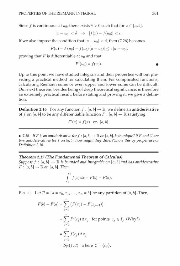
PROPERTIES OF THE RIEMANN INTEGRAL 361
Since f is continuous at u0, there exists . > 0 such that for x # [a, b],
|x " u0| < . ) |f (x) " f (u0)| < !.
If we also impose the condition that |u " u0| < ., then (7.26) becomes
|F (u) " F (u0) " f (u0) (u " u0)| + ! |u " u0|,
proving that F is differentiable at u0 and that
F &(u0) = f (u0). #
Up to this point we have studied integrals and their properties without pro-viding a practical method for calculating them. For complicated functions,calculating Riemann sums or even upper and lower sums can be difficult.Our next theorem, besides being of deep theoretical significance, is thereforean extremely practical result. Before stating and proving it, we give a defini-tion.
Definition 2.16 For any function f : [a, b] 3 R, we define an antiderivativeof f on [a, b] to be any differentiable function F : [a, b] 3 R satisfying
F &(x) = f (x) on [a, b].
! 7.28 If F is an antiderivative for f : [a, b] , R on [a, b], is it unique? If F and G aretwo antiderivatives for f on [a, b], how might they differ? Show this by proper use ofDefinition 2.16.
Theorem 2.17 (The Fundamental Theorem of Calculus)Suppose f : [a, b] 3 R is bounded and integrable on [a, b] and has antiderivativeF : [a, b] 3 R on [a, b]. Then
Y b
af (x) dx = F (b) " F (a).
PROOF Let P = {a = x0, x1, . . . , xn = b} be any partition of [a, b]. Then,
F (b) " F (a) =n+
j=1
,F (xj ) " F (xj"1)
-
=n+
j=1
F &(cj ) #xj for points cj # Ij (Why?)
=n+
j=1
f (cj) #xj
= SP (f , C) where C = {cj}.

362 REAL INTEGRATION
From this we obtain,
SP (f ) + F (b) " F (a) + SP (f ) for all partitions P of [a, b].
Therefore, Y b
af (x) dx + F (b) " F (a) +
Y b
af (x) dx.
SinceZ ba f (x) dx =
Z ba f (x) dx =
Z ba f (x) dx, it follows that
Y b
af (x) dx = F (b) " F (a).
#
! 7.29 Answer the (Why?) question in the above proof. If f has more than one an-tiderivative on [a, b], does it matter which one you use in evaluating the integral of f
over [a, b]?
! 7.30 Show that, for R > 0,Z
#
0 e!R sin %
d% <#
R. (Hint: To do so, first prove Jor-
dan’s inequality, namely, 2 %
## sin % for % " [0, #
2 ]. This in turn yieldsZ !
20 e
!R sin %d% #
Z !2
0 e"2 R "
! d%.)
In practice, the expression of the conclusion of the fundamental theorem ofcalculus is often given as
Y b
af (x) dx = F (x)
&&&b
a/ F (b) " F (a),
a notation with which students of calculus should be familiar.
Average Values
For a function f : [a, b] 3 R, the average value of f on the interval [a, b], de-noted by 0f1, might be of interest. If P is a partition of [a, b], then the averagevalue of f over [a, b] might be estimated by
1
n
n+
j=1
f (cj) where cj # Ij . (7.27)
If the partition P is chosen so that #xj = b"an for 1 + j + n, then 1
n =#xjb"a for
every 1 + j + n, and the estimate (7.27) becomes
1
b " a
n+
j=1
f (cj) #xj . (7.28)
If the function f is integrable on [a, b], letting 2P2 3 0 in (7.28) obtains thevalue
lim&P�
21
b " a
n+
j=1
f (cj) #xj
3=
1
b " a
Y b
af (x) dx.
This discussion motivates the following definition.

FURTHER DEVELOPMENT OF INTEGRATION THEORY 363
Definition 2.18 Suppose f : [a, b] 3 R is integrable on [a, b]. Then the aver-age value of f over [a, b] is given by
0f1 /1
b " a
Y b
af (x) dx.
It is an interesting fact that if f is continuous on [a, b], then f assumes itsaverage value over the interval [a, b] at some point ) # (a, b). We prove thisresult next.
Theorem 2.19 Suppose f : [a, b] 3 R is continuous on [a, b]. Then there exists) # (a, b) such that
f ()) =1
b " a
Y b
af (x) dx.
PROOF Let F : [a, b] 3 R be given by
F (u) =
Y u
af (x) dx.
Then, according to Theorem 2.15 on page 360, we know that F is continuousand differentiable on [a, b] such that F &(x) = f (x) on [a, b]. Applying the meanvalue theorem to F , we obtain
F (b) " F (a) = F &()) (b " a) for some ) # (a, b),
i.e., Y b
af (x) dx = f ()) (b" a).
#
! 7.31 For an alternative proof of the above theorem, show that the quantity given
by 1b!a
Zb
af (x) dx is between the maximum and the minimum of f on [a, b], and
apply the intermediate value theorem.
3 FURTHER DEVELOPMENT OF INTEGRATION THEORY
3.1 Improper Integrals of Bounded Functions
We sometimes wish to investigate the integrability of bounded functions overunbounded intervals. To begin, we define what it means for a function to beintegrable on an interval of the form [a,-), or ("-, b].
Definition 3.1 Suppose f : [a,-) 3 R is bounded and integrable on [a, b]
for every b > a. If the limit limb('
Z ba f (x) dx exists, then we say that f is inte-
grable on [a,!) and we denote the integral byY '
af (x) dx / lim
b('
Y b
af (x) dx.

364 REAL INTEGRATION
Similarly, suppose f : ("-, b] 3 R is bounded and integrable on [a, b] for ev-
ery a < b. If the limit lima("'
Z ba f (x) dx exists, then we say that f is integrable
on ("!, b] and we denote the integral byY b
"'f (x) dx / lim
a("'
Y b
af (x) dx.
Example 3.2 Consider f : [1,-) 3 R given by f (x) = 1x2 . Then,
Y b
1
1
x2dx = "
1
x
&&&&b
1= "
1b + 1,
and so Y '
1
1
x2dx = lim
b('
("
1b + 1
)= 1.
"
! 7.32 Evaluate the integralZ !1!%
1x2 dx.
If each of the integrals described in Definition 3.1 exists, then we considerthe function to be integrable on the whole real line. We define this formallybelow.
Definition 3.3 Suppose f : R 3 R is bounded and integrable on [a, b] forevery choice of a < b # R, and for every c # R the integrals
Z'c f (x) dx andZ c
"' f (x) dx exist. Then we say that f is integrable on R, and we denote theintegral by Y '
"'f (x) dx /
Y c
"'f (x) dx +
Y '
cf (x) dx.
! 7.33 For a function f : R , R satisfying the conditions of the above definition,show that the sum
Zc
!% f (x) dx +Z%c
f (x) dx is independent of the choice of c.
! 7.34 Suppose f : [a, b] , R is integrable on [a, b] for every choice of a, b " R, andfor a particular choice of c " R the integrals
Z %c
f (x) dx andZ
c
!% f (x) dx exist. Showthat this is enough to conclude that Definition 3.3 holds.
Example 3.4 Consider f : R 3 R given by f (x) = x e"x2. Then since f is
continuous on all of R, it follows that f is integrable on [a, b] for all a, b # R.Note that Y c
"'x e"x2
dx = lima("'
Y c
ax e"x2
dx
= lima("'
("
12 e"x2
&&&c
a
)
= lima("'
("
12 e"c2
+ 12 e"a2
)
= "12 e"c2
.

FURTHER DEVELOPMENT OF INTEGRATION THEORY 365
Similarly, Y '
cx e"x2
dx = 12 e"c2
.
Therefore, we have thatY '
"'x e"x2
dx =
Y c
"'x e"x2
dx +
Y '
cx e"x2
dx = "12 e"c2
+ 12 e"c2
= 0.
"
Example 3.5 Consider f : R 3 R given by f (x) = x. Then since f is contin-uous on all of R, it follows that f is integrable on [a, b] for all a, b # R. In thiscase, note that Y c
"'xdx = lim
a("'
Y c
axdx
= lima("'
(12 x2
&&&c
a
)
= lima("'
(12 c2
"12 a2
),
which does not exist. Therefore,Z'"' xdx does not exist. "
! 7.35 Verify that the integralZ%c
x dx does not exist either, although we do notneed this additional information in order to come to the conclusion of the previousexample.
Note that if we had computed the improper integralZ'"' xdx from the pre-
vious example somewhat differently, we would have arrived at a differentconclusion. Namely, consider the limit given by
limR('
Y R
"Rxdx = lim
R('12 x2
&&&R
"R= lim
R('
(12 R2
"12 ("R)2
)= 0.
In computing the limit in this way, we are mistakenly led to believe that theimproper integral
Z'"' xdx exists and equals 0. Note that in carrying out this
“different“ limit process, we have not used our definition for evaluating such“doubly improper“ integrals as
Z'"' xdx, namely, Definition 3.3. According
to Definition 3.3, this integral does not exist. And yet this “different“ limitprocedure is sometimes useful. We define it more formally below.
Definition 3.6 Suppose f : R 3 R is bounded and integrable on [a, b] forevery choice of a < b # R. Then, if it exists, the Cauchy principal value ofthe integral
Z'"' f (x) dx is given by the following limit,
CPV
Y '
"'f (x) dx / lim
R('
Y R
"Rf (x) dx.

366 REAL INTEGRATION
The reader is cautioned to note, as illustrated by Example 3.5, that the valueCPV
Z'"' f (x) dx may exist for a given function f even if
Z'"' f (x) dx does
not.
! 7.36 Calculate CPVZ %!% e
!|x|dx. Does
Z%!% e
!|x|dx exist? What is its relation-
ship to CPVZ%!% e
!|x|dx?
! 7.37 Show that if f : R , R is an even function thenZ%!% f (x) dx exists if and
only if CPVZ%!% f (x) dx gives the same value.
! 7.38 Show that ifZ%!% f (x) dx converges, then CPV
Z%!% f (x) dx must converge to
the same value.
3.2 Recognizing a Sequence as a Riemann Sum
We sometimes can use our acquired knowledge of integrals, paticularly inte-grable functions and their associated Riemann sums, to determine the limit-ing value of an otherwise difficult sequence. To this end, we will make use ofequality (7.3) on page 338. For example, consider the expression given by
limn('
n+
j=1
,
j
n3/2= lim
n('
C1
n3/2+
,
2
n3/2+
,
3
n3/2+ · · · +
,
n
n3/2
D
.
If we can recognize the finite sum as being a Riemann sum associated withsome integrable function f : [a, b] 3 R, we can evaluate the limit as theintegral of f over [a, b], a much simpler task in most cases than determiningthe sum directly. In our example, note that the finite sum can be rewritten as
n+
j=1
,
j
n3/2=
n+
j=1
'j
n
1
n.
This corresponds to a Riemann sum of the function f : [0, 1] 3 R given byf (x) =
,
x, with a = 0, b = 1, and #xj = 1n for each 1 + j + n. Since we know
this f is integrable over [0, 1], the limit of the sum is equal to the integralZ 10
,
xdx, that is,
limn('
n+
j=1
,
j
n3/2= lim
n('
n+
j=1
'j
n
1
n=
Y 1
0
,
xdx = 23 x3/2
&&&1
0= 2
3 .
! 7.39 What partition P of [0, 1] is implicitly used in the above Riemann sum forf (x) =
*x? Also, what set of points C is implicitly used there?
! 7.40 Find limn&%
;n
j=11n
ej/n.
! 7.41 Show that ln u = limn&%
;n
j=1u!1
n+j (u!1) .
3.3 Change of Variables Theorem
The following theorem is especially useful, as every student of calculus knows.
FURTHER DEVELOPMENT OF INTEGRATION THEORY 367
Theorem 3.7 Suppose f : [a, b] 3 R is continuous on [a, b]. Suppose g : [c, d] 3[a, b] is a function such that
(i) g(c) = a and g(d) = b, (7.29)
(ii) g& exists on [c, d] and is continuous on [c, d]. (7.30)
Then, Y b
af (x) dx =
Y d
cf (g(y)) g&(y) dy.
PROOF The proof makes explicit use of the chain rule. Let F (u) /Z ua f (x) dx.
Then F &(u) = f (u) for all u # [a, b]. Note thatd
dyF (g(y)) = F &(g(y)) g&(y) = f (g(y)) g&(y),
i.e., F (g(y)) is an antiderivative of f (g(y)) g&(y). Therefore,Y d
cf (g(y)) g&(y) dy = F (g(d)) " F (g(c))
= F (b) " F (a)
=
Y b
af (x) dx. #
In applying the above theorem, we implicitly make use of the relationshipbetween x and y given by x = g(y). The following example illustrates thetechnique, so familiar to calculus students.
Example 3.8 ConsiderZ 4
1 x ex2dx. If we let g : [1, 2] 3 [1, 4] be given by
g(y) =,
y, thenY 4
1x ex2
dx =
Y 2
1
,
y ey 12$
ydy = 1
2
Y 2
1ey dy = 1
2 (e2" e).
"
3.4 Uniform Convergence and Integration
Theorem 3.9 Suppose fn : [a, b] 3 R is a sequence of bounded integrable func-tions on [a, b] that converges uniformly to f : [a, b] 3 R. Then f is bounded andintegrable on [a, b].
PROOF We leave it to the reader to prove that f is bounded on [a, b]. Wewill establish that f is integrable. By the uniform convergence of {fn} to fon [a, b], for any ! > 0 there exists N # N such that for all x # [a, b],
n > N ) |fn(x) " f (x)| <!
2 (b " a)/ G!.

368 REAL INTEGRATION
This implies that for all x # [a, b] and for all n > N ,
fn(x) " G! < f (x) < fn(x) + G!,
and thereforeY b
a
,fn(x) " G!
-dx =
Y b
a
,fn(x) " G!
-dx +
Y b
af (x) dx
+
Y b
af (x) dx +
Y b
a
,fn(x) + G!
-dx =
Y b
a
,fn(x) + G!
-dx. (7.31)
A simple rearrangement of (7.31) yields
0 +
Y b
af (x) dx "
Y b
af (x) dx +
Y b
a
,fn(x) + G!
-dx "
Y b
a
,fn(x) " G!
-dx = !.
Since this holds for all ! > 0, it follows thatZ ba f (x) dx =
Z ba f (x) dx, and so f is
integrable on [a, b]. #
! 7.42 Complete the above proof by establishing that f is bounded on [a, b].
Theorem 3.10 Suppose fn : [a, b] 3 R is a sequence of bounded integrable func-tions on [a, b] that converges uniformly to f : [a, b] 3 R. Then,
limn('
Y b
afn(x) dx =
Y b
a
(lim
n('fn(x)
)dx =
Y b
af (x) dx.
PROOF By Theorem 3.9 we know that f is bounded and integrable on [a, b].By the uniform convergence of {fn} to f on [a, b], for any ! > 0 there existsN # N such that for all x # [a, b],
n > N ) |fn(x) " f (x)| <!
2 (b " a).
Therefore,
n > N )
&&&&&
Y b
a(fn(x) " f (x)) dx
&&&&& +!
2 (b " a)(b " a) < !. (7.32)
Expression (7.32) is equivalent to
n > N )
&&&&&
Y b
afn(x) dx "
Y b
af (x) dx
&&&&& < !,
which implies that
limn('
Y b
afn(x) dx =
Y b
af (x) dx.
#
Example 3.11 Consider the sequence of functions fn : [1, 2] 3 R given by

VECTOR-VALUED AND LINE INTEGRALS 369
fn(x) = n2 x1+n3 x2 . We know from a previous exercise that fn(x) 3 0 uniformly
on [1, 2]. Therefore, it must be true that
limn('
Y 2
1
n2 x
1 + n3 x2dx =
Y 2
1
2lim
n('n2 x
1 + n3 x2
3dx =
Y 2
10 dx = 0.
"
! 7.43 Change the domain in the previous example to [0, 1]. What happens now?
! 7.44 Let fn : [&1, 1] , R be a sequence of functions given by fn(x) = n x2
n+1+x.
a) Find limn&%
fn(x).
b) Is the convergence uniform?
c) Compute limn&%
Z 1!1 fn(x) dx and
Z 1!1
,lim
n&%fn(x)
-dx. Are they equal? Why?
Corollary 3.12 Suppose fj : [a, b] 3 R is a sequence of bounded integrable func-tions on [a, b] such that f (x) =
;'j=1 fj(x) converges uniformly on [a, b]. Then
f : [a, b] 3 R is bounded and integrable on [a, b], and,Y b
af (x) dx =
Y b
a
( '+
j=1
fj(x))dx =
'+
j=1
2Y b
afj(x) dx
3.
! 7.45 Prove the above corollary.
Example 3.13 Consider the series of functions;'
j=1sin(jx)
j5 . We know from
an exercise in Chapter 3 that this series converges uniformly on R; therefore itmust converge uniformly on ["A, A] for every choice of real number A > 0.From this, we conclude thatY A
"A
2 '+
j=1
sin(jx)j5
3dx =
'+
j=1
2Y A
"A
sin(jx)j5 dx
3=
'+
j=1
1j5
2Y A
"Asin(jx) dx
3= 0.
"
4 VECTOR-VALUED AND LINE INTEGRALS
4.1 The Integral of f : [a, b] 3 Rp
We now consider the integral of a function f : [a, b] 3 Rp, easily extendingmany of the results from the real-valued case. We begin with the followingdefinitions.

370 REAL INTEGRATION
Definition 4.1 Consider f : [a, b] 3 Rp, given by f (x) =,f1(x), . . . , fp(x)
-
where fj : [a, b] 3 R for 1 + j + p. Then, if fj is integrable on [a, b] for each1 + j + p, we say that f is integrable on [a, b], and
Y b
af (x) dx =
CY b
af1(x) dx, . . . ,
Y b
afp(x) dx
D
.
Definition 4.2 Suppose f : [a, b] 3 Rp is given by f (x) =,f1(x), . . . , fp(x)
-
where fj : [a, b] 3 R for 1 + j + p. Then we define an antiderivative of f on[a, b] to be any differentiable function F : [a, b] 3 Rp satisfying
F &(x) = f (x) on [a, b].
! 7.46 If the function F : [a, b] , Rp in the above definition is given by F (x) =,
F1(x), . . . , Fp(x)-
where Fj : [a, b] , R for 1 # j # p, show that each Fj satisfiesF
#j = fj on [a, b], and is therefore an antiderivative of fj on [a, b] for 1 # j # p.
With these definitions in hand, we state the following theorems, which areanalogous to Theorems 2.15 and 2.17 on pages 360 and 361.
Theorem 4.3 If f : [a, b] 3 Rp is bounded and integrable on [a, b], let F :[a, b] 3 Rp be the function given by
F (u) =
Y u
af (x) dx.
Then F has the following properties:
a) F is continuous on [a, b],
b) F is differentiable at points u0 # [a, b] where f is continuous,
and in this case F &(u0) = f (u0).
Note that the conclusion to part b) of the theorem can be written
d
du
2Y u
af (x) dx
3&&&&u0
= f (u0).
! 7.47 Prove the above theorem.

VECTOR-VALUED AND LINE INTEGRALS 371
Theorem 4.4 Suppose f : [a, b] 3 Rp is bounded and integrable on [a, b], andhas antiderivative F : [a, b] 3 Rp. Then
Y b
af (x) dx = F (b) " F (a).
! 7.48 Prove the above theorem.
Theorem 4.5 If f : [a, b] 3 Rp is bounded and integrable on [a, b], then |f | :[a, b] 3 R is integrable on [a, b], and
&&&&&
Y b
af (x) dx
&&&&& +Y b
a|f (x)| dx.
PROOF Let f (x) =,f1(x), . . . , fp(x)
-, where fj(x) is integrable on [a, b] for
1 + j + p. Then, by Theorems 2.7 and 2.10 on pages 354 and 357 and Exam-
ple 2.2 on page 350, |f |(x) =*
f21 (x) + · · · + f2
p (x) is integrable on [a, b]. Define
Ij /
Z ba fj(x) dx for 1 + j + p, I /
Z ba f (x)dx = (I1, I2, . . . , Ip), and note that
&&&&&
Y b
af (x) dx
&&&&&
2
=p+
j=1
CY b
afj(x) dx
D2
=p+
j=1
I2j
=p+
j=1
Y b
aIj fj(x) dx
=
Y b
a
p+
j=1
Ij fj(x) dx
=
Y b
aI · f (x) dx
+
Y b
a|I| |f (x)| dx
=
&&&&&
Y b
af (x) dx
&&&&&
Y b
a|f (x)| dx.
From this we have that &&&&&
Y b
af (x) dx
&&&&& +Y b
a|f (x)| dx.
#

372 REAL INTEGRATION
We would now like to generalize our notion of integral to include paths ofintegration other than segments of the real axis. In general, we would liketo be able to integrate a real-valued function of more than one variable f :Dk
3 R over some curve C ' Dk . There are many types of functions fto integrate, and there are many kinds of curves C to integrate over. Theproperties possessed by f and C will play a significant role in determiningthe value of such an integral.
4.2 Curves and Contours
We begin with some definitions.
Definition 4.6 Let C be a subset of Dk . If there exists a continuous functionx : [a, b] 3 Dk such that C = x
,[a, b]
-, then C is called a curve in Dk . In this
case, the function x : [a, b] 3 Dk is called a parametrization of C.
Example 4.7 Let C =.
(x, y) # R2 : x2
4 + y2
9 = 1/
. To see that C is a curve inR2, let x : [0, 2%] 3 R2 be given by x(t) = (2 cos t, 3 sin t) and note that x iscontinuous on [0, 2%]. (Why?) We will now show that x
,[0, 2%]
-= C. To see
that x,[0, 2%]
-' C, note that (2 cos t)2
4 + (3 sin t)2
9 = 1. To see that C ' x,[0, 2%]
-,
fix (x0, y0) # R2 such thatx2
04 +
y20
9 = 1. We will find at least one value of t such
that x(t) = (x0, y0). Sincex2
04 = 1 "
y20
9 + 1, it follows that "1 +x02 + 1 and
there exists t0 such that x02 = cos t0. From this we have that
y20
9= 1 "
x20
4= 1 " cos2 t0 = sin2 t0,
so that y03 = ± sin t0. This then yields
x0 = 2 cos t0 and y0 = ±3 sin t0.
If y0 = 3 sin t0 we are done, but if y0 = "3 sin t0 we have
x0 = 2 cos t0 = 2 cos("t0) and y0 = "3 sin t0 = 3 sin("t0),
and again we are done. "
It is important to note that while a given parametrization specifies a curveC ' Dk, a given curve C ' Dk has many possible parametrizations associ-ated with it. When we refer to a parametrized curve C ' Dk , we are referringto the curve along with a particular choice of parametrization x : [a, b] 3 Dk .In such a situation, the point x(a) is called the initial point of the curve, whilethe point x(b) is called the terminal point of the curve. If x(a) = x(b), the curveis called closed. If the curve does not cross itself, i.e., x(t1) $= x(t2) for alla < t1 < t2 < b, the curve is called simple. A simple closed curve is a closed

VECTOR-VALUED AND LINE INTEGRALS 373
curve whose only point of intersection is its common initial/terminal point.As an aid to visualizing a parametrized curve, each component functionxj : [a, b] 3 R of the parametrization x can be thought of as describing the j-th coordinate of some particle traversing the curve C, starting from the initialpoint x(a) and ending at the terminal point x(b). While certain parametriza-tions could allow for the particle to “backtrack“ as it moves along the curve,we will typically not use such parametrizations. For any parametrized curve,the parametrization will specify an initial and a terminal point and will si-multaneously specify a direction in which the curve is “traversed.“ Chang-ing from one parametrization to another for a given curve is referred to asreparametrizing the curve.
Example 4.8 Consider the circle of radius R centered in the plane R2. Oneparametrization of this simple closed curve is given by x : [0, 2%] 3 R2 wherex(t) = (R cos t, R sin t). The initial point is x(0) = (R, 0), the terminal point isx(2%) = (R, 0), and the circle is traversed in the counterclockwise direction."
! 7.49 Parametrize the circle described in the previous example so that it is tra-versed in the clockwise direction.
! 7.50 Suppose C in Rk is the straight line segment that connects two points p %= q
in Rk. Find a parametrization of this “curve.“
! 7.51 Let C be a curve in Rk parametrized by x : [a, b] , R
k . Let Gx : [c, d] , Rk
be given by Gx(s) = x(a + b!a
d!c(s & c)
). Show that Gx is a parametrization of C on the
parameter interval [c, d].
It is often convenient to catenate curves to form new curves.
Definition 4.9 Let {C1, C2, . . . , Cn} be a finite collection of curves in Rk withCj parametrized by xj : [j " 1, j] 3 Rk for 1 + j + n, and xj"1(j " 1) =
xj(j " 1) for 2 + j + n. Let C be the curve in Rk given by
C / (C1, C2, . . . , Cn) /n?
j=1
Cj .
When referred to as the parametrized curve C = (C1, C2, . . . , Cn), unlessspecified otherwise, we will assume C to be parametrized by x : [0, n] 3 Rk
where
x(t) =
RSSSST
SSSSU
x1(t) for 0 + t + 1,
x2(t) for 1 + t + 2,...
...
xn(t) for n " 1 + t + n.
! 7.52 Verify that the parametrized C = (C1, C2, . . . , Cn) is a curve.
It is also often convenient to subdivide a given curve into smaller curves.

374 REAL INTEGRATION
Definition 4.10 Let C be a curve in Rk with parametrization x : [a, b] 3
Rk. Let S = {!1, !2, . . . , !n#1} be any finite collection of ordered (via theparametrization) points of C, i.e., there exists a partition P = {a = t0, t1, . . . ,tn"1, tn = b}, of [a, b] such that !j = x(tj ) for 1 + j + n " 1. Define thesubcurve Cj ' C for each 1 + j + n to be the curve parametrized by xj :[tj"1, tj ] 3 C where xj(t) / x(t). We say that S subdivides C into the nsubcurves C1, C2, . . . , Cn, which form a subdivision of C.
Note from the above definition that C1 is that part of C from x(a) to !1, C2
is that part of C from !1 to !2, and so on. Note too, that any partition speci-fied for a given parametrized curve implicitly provides a subdivision of thatcurve. Also, by selecting a set of (ordered) points S = {!1, . . . , !n#1} from agiven parametrized curve C, one has also selected a partition P of [a, b].
Both S and the associated P subdivide C into C1, C2, . . . , Cn, and clearly wemay write C = (C1, C2, . . . , Cn).
Of particular importance in our work will be the kinds of curves known assmooth curves.
Definition 4.11 Let C be a curve in Dk . If there exists a parametrizationx : [a, b] 3 Dk such that
(i) x is continuously differentiable on [a, b],
(ii) x&(t) $= 0 for all t # [a, b],
then C is called a smooth curve in Dk .
Condition 2, that x&(t) not vanish on [a, b], distinguishes a smooth curve fromone that is merely continuously differentiable. Recall the definition of theunit tangent vector to a curve from calculus, and the imposition of this con-dition becomes a bit clearer. Consider a curve in R2 as an example, withparametrization x(t) = (x(t), y(t)) for a + t + b. If we think of x(t) as indi-cating a particle’s position in the plane at any time t # [a, b], the unit tangentvector to the path of this particle is given by
[T =x&(t)
|x&(t)|,
which would clearly be undefined if x&(t) were zero. A smooth curve is onewhose unit tangent vector is well defined along the entire curve and thatchanges its direction, that is, its angle of inclination with the positive realaxis, in a continuous manner.
We now define what we will call a contour.

VECTOR-VALUED AND LINE INTEGRALS 375
Definition 4.12 Let C be a curve in Dk . If there exists a parametrizationx : [a, b] 3 Dk and a partition P = {a = t0, t1, . . . , tn = b} of [a, b] such thatCj / x
,[tj"1, tj]
-is a smooth curve for 1 + j + n, then C is called a contour.
A contour C in Dk is a curve that is the union of a finite number of smoothcurves Cj ' Dk . If x : [a, b] 3 Dk is a parametrization of the contourC consistent with Definition 4.12, then for each 1 + j + n the functionxj : [tj"1, tj] 3 Dk given by xj(t) / x(t) is the induced parametrization of thesmooth curve Cj . Note that the initial point of Cj coincides with the terminalpoint of Cj"1 for every 1 + j + n. Clearly, the initial point of C1 and theterminal point of Cn are the initial and terminal points of the contour C, andso, C = (C1, C2, . . . , Cn). Also, there are such things as closed contours (thosefor which the initial point of C1 coincides with the terminal point of Cn),simple contours (those that have no points of self-intersection other than pos-sibly the initial and terminal points coinciding), and smooth contours (thosethat are smooth curves). It is worth noting that with respect to this lattercategory, “patching“ smooth curves together to form contours will not nec-essarily result in a smooth contour. The “patch points“ will not in general bepoints with well-defined derivatives. The following example illustrates howtwo smooth curves can be patched together to form a contour.
Example 4.13 Consider the contour C in R2 shown in Figure 7.2 below. LetC1 be the smooth curve parametrized by x1 : [0, %] 3 R2 where x1(t) =(R cos t, R sin t), and let C2 be the smooth curve parametrized by x2 : [%, % +2 R] 3 R2 where x2(t) = (t " % " R, 0). Then the contour C = (C1, C2) isparametrized by x : [0, % + 2 R] 3 R2 given by
x(t) =
Ex1(t) for 0 + t + %,
x2(t) for % + t + % + 2 R.
Note that C is not smooth.
C1
C2!R R
C
"
Figure 7.2 The semicircular contour C.

376 REAL INTEGRATION
! 7.53 Find another parametrization for the contour C described above such thatthe initial and terminal points are both (&R, 0).
For a given contour C in Dk it will be useful to define when two parametriza-tions of C are equivalent in a certain sense. We begin by defining when twoparametrizations of a smooth curve are equivalent.
Definition 4.14 Let C be a smooth curve in Dk with parametrization x :[a, b] 3 Dk. Another parametrization of C given by Gx : [c, d] 3 Dk is calledequivalent to x if there exists a mapping g : [c, d] 3 [a, b] such that
(i) Gx = x ; g,
(ii) g is C1 on [c, d],
(iii) g& > 0 on [c, d],
(iv) g(c) = a and g(d) = b.
Loosely speaking, two parametrizations of a contour C are equivalent if theyassociate the same initial and terminal points, and if they preserve the direc-tion in which the contour is traversed as the parameter increases. In terms ofan imagined particle traversing the contour, the difference between two dif-ferent but equivalent parametrizations can be likened to the particle travers-ing the contour at different speeds. It is useful to know how to reparametrizea given contour, that is, to change from a given parametrization to a differentone.
! 7.54 Let C be a smooth curve in Dk with parametrization x : [a, b] , D
k . Letg : [c, d] , [a, b] be such that properties 2–4 of Definition 4.14 hold. Show that Gx :
[c, d] , Dk given by Gx = x 3 g is a parametrization of C and is therefore equivalent
to x.
We can easily define two contour parametrizations to be equivalent in the sameway that two curve parametrizations are defined to be equivalent, namely, xand Gx are equivalent if Gx = x ; g for a function g as above.
Example 4.15 Consider again the circle of radius R centered in the planeR2 and parametrized by x : [0, 2%] 3 R2 where x(t) = (R cos t, R sin t). Letg : [0, %] 3 [0, 2%] be given by g(s) = 2 s. Then Gx : [0, %] 3 R2 given byGx(s) = x ; g(s) =
,R cos(2s), R sin(2s)
-is a reparametrization of C. Recall
from vector calculus that the instantaneous velocity of an imagined particleas it traverses the curve C according to the original parametrization is givenby x&(t). Its instantaneous speed is the magnitude of this velocity, which inthis case is just R. We leave it to the reader to verify that a particle traversingthis curve according to the reparametrization does so twice as fast as withthe original parametrization, but traverses it in the same direction, and withthe same initial and terminal points. Therefore, this new parametrization isequivalent to the original one. "

VECTOR-VALUED AND LINE INTEGRALS 377
! 7.55 Confirm the claim in the above example. Then reparametrize the curve sothat an imagined particle traverses it three times more slowly than the original parametriza-tion.
! 7.56 Consider the contour C described in Example 4.13 above. Find an equivalentreparametrization of C.
It can also be useful to traverse a given parametrized contour C “in reverse.“To this end, let C be a given parametrized contour having initial and terminalpoints x(a) and x(b), respectively. We define the parametrized contour "C tobe the same set of points as C, but with initial point x(b), terminal point x(a),and parametrized so as to be traversed in the “opposite“ direction from theparametrized contour C. The following result establishes a convenient wayto obtain a parametrization for "C with these properties.
Theorem 4.16 Suppose C is a contour in Dk with parametrization xC : [a, b] 3Dk. Then x"C : ["b,"a] 3 Dk given by
x"C (t) = xC ("t)parametrizes the contour "C.
! 7.57 Prove the above theorem. Begin by considering the case where C is a smoothcurve.
Example 4.17 Let C ' R2 be the circle parametrized by xC : [0, 2%] 3 R2
where xC (t) = (r cos t, r sin t). Then "C is the circle parametrized by x"C :["2%, 0] 3 R2 where x"C (t) =
,r cos("t), r sin("t)
-= (r cos t,"r sin t). The
reader should verify that x"C parametrizes the circle in the clockwise direc-tion, whereas xC parametrized the circle in the counterclockwise direction."
! 7.58 Verify the above.
4.3 Line Integrals
We begin our discussion of line integrals with the following definition.
Definition 4.18 Let f : Dk3 R be continuous on the open set Dk
' Rk andlet C be a smooth curve in Dk with parametrization x : [a, b] 3 Dk givenby x(t) =
,x1(t), . . . , xk(t)
-. For each 1 + j + k, the line integral of f with
respect to xj is given by
Y
C
f (x1, . . . , xk) dxj /
Y b
af,x1(t), . . . , xk(t)
-x&j (t) dt.

378 REAL INTEGRATION
If C = (C1, . . . , Cn) is a contour in Dk , then for each 1 + j + k,Y
C
f (x1, . . . , xk) dxj /
n+
)=1
Y
C$
f (x1, . . . , xk) dxj .
! 7.59 Let f , g : Dk , R be continuous on the open set D
k , and suppose C is a
contour in Dk . Show the following:
a)Z
C
(f ± g)(x) dxj =Z
C
f (x) dxj ±Z
C
g(x) dxj for each 1 # j # k.
b) For any ! " R,Z
C
! f (x) dxj = !Z
C
f (x) dxj for each 1 # j # k.
Example 4.19 Let C = (C1, C2) be the piecewise-smooth contour describedin Example 4.13, and let f : R2
3 R be given by f (x, y) = x2 + y2. Then,Y
C1
f (x, y) dx =
Y $
0R2 ("R sin t)dt = "2 R3,
and Y
C2
f (x, y) dx =
Y $+2 R
$(t " % " R)2 dt = 2
3 R3.
Therefore,Y
C
f (x, y) dx =
Y
C1
f (x, y) dx +
Y
C2
f (x, y) dx = "2 R3 + 23 R3 = "
43 R3.
"
! 7.60 FindZ
C
f (x, y) dy for the previous example.
The following theorem is an especially useful result. We leave its proof to thereader.
Theorem 4.20 Suppose f : Dk3 R is continuous on the open set Dk
' Rk
and C is a contour in Dk with parametrization x : [a, b] 3 Dk given by x(t) =,x1(t), . . . , xk(t)
-. Suppose Gx : [c, d] 3 Dk given by Gx(t) =
,Gx1(t), . . . , Gxk(t)
-is a
parametrization of C equivalent to x. Then for each 1 + j + k,Y
C
f (x1, . . . , xk) dxj =
Y
C
f (Gx1, . . . , Gxk) dGxj .
! 7.61 Prove the above theorem, considering first the case where C is a smoothcurve.
Example 4.21 Let f : R23 R be given by f (x, y) = x2 +xy+1, and let C ' R2
be the contour parametrized by x : [0, 1] 3 R2 where x(t) = (t, t2). Then,

VECTOR-VALUED AND LINE INTEGRALS 379
Y
C
f (x, y) dx =
Y 1
0(t2 + t3 + 1) dt = 19
12 .
If we let g : ["1, 0] 3 [0, 1] be given by g(s) = s3 + 1, then by Definition 4.14on page 376 it follows that Gx : ["1, 0] 3 R2 given by
Gx(s) / x,g(s)
-=,s3 + 1, (s3 + 1)2-
is an equivalent parametrization of C. RecalculatingZ
C
f (x, y) dx with the equiv-
alent parametrization Gx obtainsY
C
f (Gx, Gy) dGx =
Y 0
"1
A(s3 + 1)2 + (s3 + 1)3 + 1
B3s2 ds = 19
12 ,
the same value as with the original parametrization. "
! 7.62 Show thatZ
C
f (x, y) dy =Z
C
f (Gx, Gy) dGy in the above example.
For the most general line integral, consider the following definition.
Definition 4.22 Let f : Dk3 Rk be continuous on the open set Dk
' Rk
with f = (f1, . . . , fk), and let C be a smooth curve in Dk with parametrizationx : [a, b] 3 Dk given by x(t) =
,x1(t), . . . , xk(t)
-. Then the line integral of f
with respect to x along C is given byY
C
f (x) · dx /
Y
C
f1(x) dx1 + · · · + fk(x) dxk /
Y
C
f1(x) dx1 + · · · +
Y
C
fk(x) dxk.
Note that the above, in combination with the chain rule, yieldsY
C
f (x) · dx /
Y
C
f1(x) dx1 + · · · + fk(x) dxk
=
Y
C
f1(x) dx1 + · · · +
Y
C
fk(x) dxk
=
Y b
af1(x(t))
dx1
dtdt + · · · +
Y b
afk(x(t))
dxk
dtdt
=
Y b
a
2f1(x(t))
dx1
dt+ · · · + fk(x(t))
dxk
dt
3dt
=
Y b
af (x) ·
dx
dtdt. (7.33)
The formula for the line integral indicated by (7.33) is often useful in appli-cations. It also leads to the following nice result.

380 REAL INTEGRATION
Theorem 4.23 (The Fundamental Theorem of Calculus for Line Integrals)Suppose f : Dk
3 Rk is continuous on the open set Dk' Rk with f = (f1, . . . , fk),
and let C be a contour in Dk with parametrization x : [a, b] 3 Dk given byx(t) =
,x1(t), . . . , xk(t)
-. Suppose also that there exists F : Dk
3 R such that
f = %F on Dk. Then,Y
C
f (x) · dx = F,x(b)
-" F
,x(a)
-.
! 7.63 Prove the above theorem.
The above theorem is a generalization of the fundamental theorem of calcu-lus, and it is a great convenience. It implies two very interesting facts. First,under the right circumstances, the value of the line integral of a vector-valuedfunction f along a contour C can be obtained simply by evaluating the func-tion’s antiderivative at the endpoints of the contour. Second, if the contour C isclosed, then the value of the line integral is zero.
! 7.64 Is it necessary that the function F : Dk , R referred to in Theorem 4.23 be
differentiable, i.e., is it necessary that f be the derivative of F ?
Example 4.24 Let f : R33 R3 be given by f (x, y, z) = (yz, xz, xy), and let
C ' R3 be the contour parametrized by x : [0, 1] 3 R3 where x(t) = (t, t2, t3).Then,
Y
C
f (x) · dx =
Y
C
yz dx + xz dy + xy dz
=
Y 1
0t5 dt +
Y 1
0t4 (2t) dt +
Y 1
0t3 (3t2) dt
=
Y 1
06t5 dt = 1.
Note, however, that since f has an antiderivative F : R33 R given by
F (x, y, z) = xyz, we haveY
C
f (x) · dx = F,x(1)
-" F
,x(0)
-= F (1, 1, 1) " F (0, 0, 0) = 1,
which is much easier. "
! 7.65 Verify that the function F in the above example is an antiderivative for thefunction f given there.
The following theorem tells us how a line integral changes when we traversea contour C in the opposite direction.

SUPPLEMENTARY EXERCISES 381
Theorem 4.25 Suppose f : Dk3 R is continuous on Dk and that C is a contour
in Dk. Then,Y
"C
f (x1, . . . , xk) dxj = "
Y
C
f (x1, . . . , xk) dxj .
PROOF We consider the case where C is a smooth curve and leave the moregeneral case to the reader. If xC : [a, b] 3 Dk given by xC (t) =
,x1(t), . . . , xk(t)
-
is a parametrization of C, then x"C : ["b,"a] 3 Dk given by x"C (t) =,x1("t), . . . , xk("t)
-is a parametrization of "C. From this we have that
Y
"C
f (x1, . . . , xk) dxj =
Y "a
"bf,x1("t), . . . , xk("t)
- ," x&j ("t)
-dt.
Changing variables by letting s = "t, we obtainY
"C
f (x1, . . . , xk) dxj =
Y a
bf,x1(s), . . . , xk(s)
- ," x&j (s)
-("ds)
= "
Y b
af,x1(s), . . . , xk(s)
-x&j (s) ds
= "
Y
C
f (x1, . . . , xk) dxj . #
! 7.66 Prove the above theorem for contours.
Example 4.26 Let f : R23 R be given by f (x, y) = x2 + y2, and C be the
curve in R2 parametrized by xC (t) = (R cos t, R sin t) for t # [0, %]. Then "Cis parametrized by x"C (t) = (R cos t,"R sin t) for t # ["%, 0], and
Y
C
(x2 + y2) dx =
Y $
0R2 ("R sin t) dt = "2 R3,
while Y
"C
(x2 + y2) dx =
Y 0
"$R2 ("R sin t) dt = 2 R3.
"
5 SUPPLEMENTARY EXERCISES
1. Recall that we appended our definition of the integrability of f : [a, b] , R givenin Definition 1.5 on page 337 with the seemingly arbitrary definition (7.1), repeatedhere for convenience: Y
a
b
f (x) dx . &Y
b
a
f (x) dx. (7.1)

382 REAL INTEGRATION
This exercise will help the reader to justify this definition. In particular, note thatin defining the Riemann sum associated with the integral of f from a to b, one canthink of the Riemann sum, and hence the associated integral, as accumulating valuesas you traverse the interval [a, b] from a to b, left-to-right along the x-axis. We haddefined the length of each subinterval Ij as #xj = xj & xj!1, a natural definitionthat assigns a positive length to each subinterval Ij since xj!1 < xj . Using the samepoints C and subintervals {Ij} defined by P = {a = x0, x1, . . . , xn = b} from before,one could also determine the integral obtained by traversing the interval [a, b] in theopposite direction, from b to a, or right-to-left along the x-axis. Since a partition is anordered set of points from the interval [a, b], we are now effectively making use ofthe “reverse“ partition Pr = {xr
0 , xr
1 , . . . , xrn} = {b = xn, xn!1 . . . , x0 = a}. From this,
we see that #xr
j = xr
j & xr
j!1 = xn!(j!1) & xn!j = &(xn!j & xn!(j!1)) = &#xn!j .The reader should verify that the resulting Riemann sum associated with Pr is thesame in magnitude as that associated with P , but opposite in sign. This results in theformula given by (7.1).
2. Use the result of the previous exercise to justify the definition given by (7.2) onpage 338, i.e.,
Z c
cf (x) dx . 0, for any c " [a, b].
3. Suppose f : [a, b] , R is nonnegative and continuous on [a, b] such thatZ b
af (x) dx =
0. Show that f . 0 on [a, b].
4. Suppose f " C2,[a, b]
-, and that f (x) ' 0 and f
##(x) # 0 on [a, b]. Show that
12 (b & a)
,f (a) + f (b)
-#
Yb
a
f (x) dx # (b & a) f
(a+b
2
).
5. Integration by parts. Suppose u, v : [a, b] , R are differentiable on [a, b], and u#
and v# are integrable on [a, b]. Show that
Yb
a
u(x) v#(x) dx = u(x) v(x)
&&ba&
Yb
a
v(x) u#(x) dx.
6. EvaluateZ 2
13*
x dx using Definition 1.5 on page 337.
7. EvaluateZ 2
0
,x + |x & 1|
-dx.
8. Let f : [0, 3] , R be given by f (x) =
RST
SU
x on [0, 1]
x & 1 on (1, 2]
0 on (2, 3]
. Define F : [0, 3] , R by
F (u) =Z
u
0 f (x) dx. Is F continuous? Does F# = f on all of [0, 3]?
9. Let f : [a, b] , R be bounded and integrable, and suppose g : [a, b] , R is suchthat g(x) = f (x) on [a, b] except at a finite number of points of [a, b]. Show that g is
also integrable on [a, b], and findZ b
ag(x) dx.
10. The function g to which we referred in the previous exercise is not necessarilyintegrable if g(x) %= f (x) on Q $ [a, b]. To see this, construct such a g : [a, b] , R and

SUPPLEMENTARY EXERCISES 383
show that it is not integrable on [a, b]. Suppose g(x) %= f (x) on some infinite collection
of points within [a, b]. Is it necessarily true thatZ
b
af (x) dx %=
Zb
ag(x) dx?
11. Suppose f : [0, 1] , R is continuous on [0, 1] andZ u
0 f (x) dx =Z 1u
f (x) dx forevery u " [0, 1]. Find f (x).
12. Suppose f : [a, b] , R is continuous on [a, b] andZ
b
af (x) dx = 0. Show that there
exists c " [a, b] such that f (c) = 0.
13. Find an example of a function f : [a, b] , R such that f is not integrable on [a, b],but |f | and f
2j are for any j " N.
14. Suppose f : [a, b] , R is continuous on [a, b] such that |f (x)| # 1 on [a, b], andZb
af (x) dx = b & a. Show that f (x) . 1 on [a, b].
15. Find an integrable function f : [0, 1] , R such that F : [a, b] , R given byF (u) =
Zu
0 f (x) dx does not have a derivative at some point of [a, b]. Can you find anf such that F is not continuous at some point of [a, b]?
16. Let f : [0, 1] , R be given by f (x) =
Ex
2 sin(
1x2
)if x %= 0 and x " [0, 1]
0 if x = 0. Show
that f is differentiable on [0, 1], but f# is not integrable on [0, 1]. Clearly f
# can’t becontinuous on [0, 1], right?
17. Let C be the Cantor set, and define 0C : [0, 1] , R, the characteristic func-
tion of C, by 0C (x) =
E1 for x " C $ [0, 1]
0 for x %" C $ [0, 1]. Show that 0C is integrable and that
Z 10 0C (x) dx = 0. Contrast this with Example 1.18 on page 349. How does 0C differ
from the function described there? How are they similar?
18. Suppose f : [a, b] , R is continuous on [a, b], and thatZ
b
af (x) h(x) dx = 0 for
every continuous h : [a, b] , R. Show that f . 0 on [a, b].
19. Suppose f : [a, b] , R is integrable on [a, b], and thatZ b
af (x) h(x) dx = 0 for
every continuous h : [a, b] , R. Show that f (x) = 0 at all points x " [a, b] where f iscontinuous.
20. Suppose f : [a, b] , R is integrable on [a, b], and g : R , R is continuous on R.Is g 3 f : [a, b] , R necessarily integrable?
21. Show that limn&%
Z b
0 e!nx
dx = 0 for any choice of b > 0. Now answer the fol-
lowing with a valid explanation: The sequence of functions fn(x) = e!nx converges
uniformly on [0, b], true or false?
22. Suppose 0 < a < 2. Show that limn&%
Z 2a
e!nx
dx = 0. Now consider the case a = 0.

384 REAL INTEGRATION
23. Leibniz’s ruleLet f : [a, b] , R be a bounded and integrable function on [a, b], and let g, h : D
1 ,[a, b] be differentiable on D
1. Show the following.
a) The function F : D1 , R given by F (u) =
Zg(u)a
f (x) dx is differentiable at
points u0 " D1 where f is continuous, and F
#(u0) = f,g(u0)
-g#(u0).
b) The function G : D1 , R given by G(u) =
Z g(u)h(u) f (x) dx is differentiable at
points u0 " D1 where f and g are continuous. Find G
#(u).
c) Generalize the above results to the case of f : [a, b] , Rp, where
f (x) =,f1(x), . . . , fp(x)
-and fj : [a, b] , R for 1 # j # p.
24. Let;%
n=1 xn be a series of positive nonincreasing real numbers, and supposef : [N , /) , R is a function such that f (n) = xn for n ' N . Show that
;%n=1 xn andZ%
Nf (x) dx both converge or both diverge.
25. Improper integrals of unbounded functionsLet f : (a, b] , R be such that f is integrable on [c, b] for every a < c < b, and
limx#a+
f (x) = ±/. We define the improper integralZ
b
af (x) dx = lim
c&a+
Zb
cf (x) dx when
this limit exists. Similarly, suppose g : [a, b) , R is integrable on [a, c] for every a <
c < b, and limx&b"
g(x) = ±/. Define the improper integralZ
b
ag(x) dx = lim
c&b"
Zc
ag(x) dx
when this limit exists. Show thatZ 1
01"x
dx exists, butZ 1
01x
dx does not.
26. Integrals depending on a parameterLet D
2 = [a, b] + [c, d] and suppose f (x, t) is continuous on D2. Define F : [c, d] , R
by F (t) .Z b
af (x, t) dx.
a) Show that F is continuous on [c, d].
b) Suppose (f
(tand (f
(xare continuous on D
2. Show that F is differentiable on
[c, d], and F#(t0) =
Z b
a
(f
(t(x, t0) dx.
27. The Cauchy-Schwarz inequality for integrals
a) If a, b " R, show that ab # a2+b
2
2 .
b) Given Riemann-integrable functions f , g : [a, b] , R, show thatY
b
a
|f (x)g(x)|dx # 12
CYb
a
f (x)2dx +
Yb
a
g(x)2dx
D
.
c) Show that ifZ
b
af (x)2
dx =Z
b
ag(x)2 = 1, then
Zb
a|f (x)g(x)|dx # 1.
d) Show that for any f , g,Y b
a
|f (x)g(x)|dx #
CY b
a
f (x)2dx
D1/2 CY b
a
g(x)2dx
D1/2
.
To do this, note that it is true when both factors on the right are 1 (Why?). Observethat the inequality is homogeneous in f and g, i.e., you can divide f or g by aconstant factor and it will still hold. And when one of those is zero, this is trivial(Why?).

SUPPLEMENTARY EXERCISES 385
e) Look back at Chapter 1 at the section on inner products. Prove that
(f , g) =
Yb
a
f (x)g(x)dx
is an inner product on the vector space of continuous functions on [a, b]. Does theproof of the Cauchy-Schwarz inequality there still work? What does the triangleinequality state here, if it works?
28. A function 1 : R , R is called convex when 1(w1x1 + w2x2 + · · · + wnxn) #w11(x1) + w21(x2) + · · · + wn1(xn). Suppose f : [0, 1] , R is continuous. Show that
1
CY 1
0f (x)dx
D
#Y 1
01(f (x))dx,
a statement known as Jensen’s inequality by considering Riemann sums whose normsare very small, and applying the definition of a convex function.
29. This exercise and the next illustrate useful techniques in analysis, cf. [Zyg77]. Letf : [a, b] , R be continuous. Define the sequence {fn} as
fn =
Y b
a
f (x) sin(nx)dz. (7.34)
In this exercise you will prove a version of the Riemann-Lebesgue lemma, i.e., thatlim fn = 0.
a) Suppose g is the characteristic function of a subinterval I# of [a, b], i.e., g(x) = 1
if x " I#, and g(x) = 0 otherwise. Define the sequence gn correspondingly, as in
(7.34). Prove by direct calculation that lim gn = 0.
b) Prove the same when g is a step function, or a linear combination of characteristicfunctions of intervals.
c) Given $ > 0 and f continuous, prove that there exists a step function g such that|f (x) & g(x)| < $ for all x " [a, b]. Deduce that |fn| # |gn| + $(b & a).
d) Show that lim sup |fn| # $(b & a) and finish the proof.
30. Let f : [0, 1] , R be nonnegative and continuous. Write M = sup[0,1] f . Considerthe expressions
Mn =
CYb
a
fndx
D1/n
for each n " N.a) Prove that Mn # M for all n.
b) Fix $ > 0. Prove that there exists an interval J = [c & ), c + )] ! [0, 1] such thatf (x) > M & $ for x " J .
c) Prove that (with the same notation) Mn ' (2))1/n(M&$). Deduce that lim inf Mn 'M & $.
d) Prove that lim Mn = M .


8COMPLEX INTEGRATION
The shortest path between two truths in the real domain passes through the complexdomain.
Jacques Hadamard
We have already seen how complex functions can have significantly differentproperties than real-valued or vector-valued functions. Not the least of theseare the very different and far-reaching implications associated with complexdifferentiability. The theory of complex integration is no less rich. Some ofthe results we ultimately develop will rely on subtle topological propertiesof certain subsets of the plane, as well as the curves along which we will in-tegrate. In fact a proper development of the main theorem of this chapter,Cauchy’s integral theorem, will require quite a bit of careful effort due tosuch subtleties. Despite this, we will find that integration is as useful an an-alytical tool as differentiation for investigating complex functions and theirkey properties. In fact it is in the theory of complex integration where we willdiscover some of the most interesting and useful results in all of analysis, re-sults that will apply even to real functions of a real variable.
1 INTRODUCTION TO COMPLEX INTEGRALS
1.1 Integration over an Interval
We begin by considering the integral of a continuous complex-valued func-tion of a single real variable, w : [a, b] 3 C. We assume w has the formw(t) = u(t) + iv(t), and so w being continuous implies that each of u and v iscontinuous. We define the integral of w(t) on [a, b] according to
Y b
aw(t) dt /
Y b
au(t) dt + i
Y b
av(t) dt. (8.1)
This definition is consistent with the linearity property possessed by the inte-gral of a real-valued function of a single real variable, extended in the natural
387

388 COMPLEX INTEGRATION
way to include pure imaginary constants. We will build on this basic defini-tion, developing for our complex integral many of the properties possessedby the more familiar integral of real-valued functions. Consistent with this,we define the complex integral from b to a where a < b according to
Y a
bw(t) dt / "
Y b
aw(t) dt,
and the complex integral from c to c for any c # [a, b] according toY c
cw(t) dt / 0.
The following result should also be familiar from the real case.
Proposition 1.1 Suppose w, w1, w2 : [a, b] 3 C are continuous on [a, b].
a) If z1, z2 # C, thenZ ba
,z1 w1(t) + z2 w2(t)
-dt = z1
Z ba w1(t) dt + z2
Z ba w2(t) dt.
b) Re(Z b
a w(t) dt)
=Z ba Re
,w(t)
-dt, and Im
(Z ba w(t) dt
)=Z ba Im
,w(t)
-dt.
c) If c1, c2, and c3 are any three points from [a, b], then,Y c2
c1
w(t) dt =
Y c3
c1
w(t) dt +
Y c2
c3
w(t) dt.
! 8.1 Prove the above proposition.
Some of the most useful results in analysis aren’t identities or equalities, theyare inequalities. Such results are particularly useful in proving theorems, andone such inequality, a sort of “triangle inequality for line integrals“ follows.
Theorem 1.2 Suppose w : [a, b] 3 C is continuous on [a, b], with " / max[a,b]
|w(t)|.
Then,&&&&
Y b
aw(t) dt
&&&& +Y b
a
&&w(t)&& dt + " (b " a).
PROOF IfZ ba w(t) dt = 0, we are done. Therefore assume that
Z ba w(t) dt =
r0 ei"$= 0. Then we have
&&&&
Y b
aw(t) dt
&&&& = r0 = Re(r0) = Re(e"i" r0 ei"
)
= Re
2e"i"
Y b
aw(t) dt
3
= Re
2Y b
ae"i" w(t) dt
3
=
Y b
aRe
,e"i" w(t)
-dt

INTRODUCTION TO COMPLEX INTEGRALS 389
+
Y b
a
&&e"i" w(t)&& dt
=
Y b
a
&&w(t)&& dt.
Clearly,Z ba
&&w(t)&& dt + " (b " a), and the theorem is proved. #
In the above theorem it is often more convenient to replace " with any M !
". This is particularly true when any upper bound is all that is needed, orwhen the maximum of |w(t)| over [a, b] is inconveniently obtained.
The following result is the familiar change-of-variables formula from calcu-lus in terms of our new complex integral.
Proposition 1.3 Suppose w : [a, b] 3 C is continuous on [a, b], and let t = g(s)where g : [c, d] 3 [a, b] has the following properties:
(i) g(c) = a and g(d) = b,
(ii) g is continuously differentiable on [c, d].
Then, Y b
aw(t) dt =
Y d
cw(g(s)) g&(s) ds.
! 8.2 Prove the above proposition.
What would our complex integral be worth if the fundamental theorem ofcalculus didn’t apply? It does, as described by the following results.
Proposition 1.4 Suppose w : [a, b] 3 C is continuous on [a, b] and W : [a, b] 3C is given by
W (s) =
Y s
aw(t) dt.
Then W is differentiable on [a, b], and W &(s) = w(s) for all s # [a, b].
The careful reader will notice that we never formally defined what it meansfor a function W : [a, b] 3 C to be differentiable. But the definition is trans-parent. If we write W = U + iV for real-valued functions U , V , then W &(t) =w(t) just means U &(t) = Re(w(t)) and V &(t) = Im(w(t)).
! 8.3 Prove the above proposition.

390 COMPLEX INTEGRATION
Theorem 1.5 (The Fundamental Theorem of Calculus)Suppose w : [a, b] 3 C is continuous on [a, b], and there exists a differentiablecomplex-valued function W : [a, b] 3 C such that W &(t) = w(t) on [a, b]. Then,
Y b
aw(t) dt = W (t)
&&&b
a= W (b) " W (a).
PROOF Let w(t) = u(t) + iv(t) and W (t) = U (t) + iV (t), where U &(t) = u(t) andV &(t) = v(t) for all t # [a, b]. Then by definition of our complex integral andthe fundamental theorem of calculus for real functions, we have
Y b
aw(t) dt =
Y b
au(t) dt + i
Y b
av(t) dt
=,U (b) " U (a)
-+ i
,V (b) " V (a)
-
= W (b) " W (a). #
As a simple illustration of the above, consider w : [0, 1] 3 R given by w(t) =t2 + i t3. Then,
Y 1
0w(t) dt =
Y 1
0(t2 + i t3) dt =
(13 t3 + i 1
4 t4) &&&
1
0= 1
3 + i 14 .
1.2 Curves and Contours
In general, we would like to be able to integrate a complex-valued functionof a complex variable over a curve C in the complex plane. To begin, weextend our notion of a parametrized curve from R2 to C in the natural way.Recall that a curve C in R2 can be parametrized by a continuous map x :[a, b] 3 R2. Similarly, we will say that a curve C in C can be parametrized bya continuous map z : [a, b] 3 C. In this case, z(a) is referred to as the initialpoint of the curve C and z(b) is referred to as the terminal point of the curveC. The curve C = (C1, . . . , Cn) =
#nj=1 Cj is to be interpreted in C as in R2, as
a union of curves Cj for 1 + j + n, or, when parametrized, as a catenationof curves Cj for 1 + j + n. The notion of equivalent parametrizations for agiven curve C in C is also defined as in the real case, as are the definitionsfor closed curve, simple curve, and smooth curve. In particular, the curve Cin C is smooth if there exists a parametrization z : [a, b] 3 C such that zis continuously differentiable on [a, b] and z&(t) $= 0 for all t # [a, b]. Finally,contours are also defined as in the real case. A contour C&
' C will be called asubcontour of the contour C ' C if every point of C& is also a point of C, i.e.,C&
' C.
Circles
The following definitions and conventions will also be of use to us in whatfollows.

INTRODUCTION TO COMPLEX INTEGRALS 391
Definition 1.6 For any r > 0 and z0 # C, let Cr(z0) be the circle in C havingradius r and center z0, i.e.,
Cr(z0) / {z # C : |z " z0| = r}.
When referred to as the parametrized circle Cr(z0), unless specified other-wise, we will assume Cr(z0) to be parametrized by z : [0, 2 %] 3 C where
z(t) = z0 + r ei t.
! 8.4 Verify that the parametrized circle Cr(z0) is a smooth curve, and that the de-fault parametrization described in Definition 1.6 associates a counterclockwise direc-tion to the traversal of Cr(z0).
! 8.5 Fix %0 " R. Let Gz : [%0, %0 + 2 '] , C be given by Gz(t) = z0 + r ei t. Show that
Gz is also a parametrization of Cr(z0). How does Cr(z0) parametrized by Gz differ fromCr(z0) parametrized by z?
Line Segments and Polygonal Contours
Definition 1.7 For any z1, z2 # C with z1 $= z2, let [z1, z2] ' C be the closedline segment in C determined by z1 and z2. When referred to as the parametrizedsegment [z1, z2], unless specified otherwise, we will assume [z1, z2] to beparametrized by z : [0, 1] 3 C where
z(t) = z1 + t (z2 " z1).
! 8.6 Verify that the parametrized segment [z1, z2] is a smooth curve with initialpoint z1 and terminal point z2.
! 8.7 Let Gz : [a, b] , C be given by Gz(t) = z1 + t!a
b!a(z2 & z1). Show that Gz is a
parametrization of [z1, z2] that is equivalent, according to Definition 4.14 in Chapter7, to the parametrization z given in Definition 1.7.
Definition 1.8 The collection of points {z0, z1, z2, . . . , zN} ' C are calledvertices if they have the following properties:
1. zj"1 $= zj for 1 + j + N ,
2. zj"1, zj , zj+1 for 1 + j + N " 1 are not collinear.
Let P be the polygonal contour in C given by
P / [z0, z1, . . . , zN ] /N?
j=1
[zj"1, zj].
When referred to as the parametrized polygonal contour P , unless specified

392 COMPLEX INTEGRATION
otherwise, we will assume P to be parametrized by z : [0, N ] 3 C where
z(t) =
RSSSST
SSSSU
z0 + t (z1 " z0) for 0 + t + 1,
z1 + (t " 1) (z2 " z1) for 1 + t + 2,...
...
zN"1 +,t " (N " 1)
-(zN " zN"1) for N " 1 + t + N .
z1
z2
z3
z0
z4
z5
Figure 8.1 A polygonal contour.
The condition that zj"1 $= zj for 1 + j + N in the above definition simply en-sures that no point is repeated consecutively in the collection {z0, z1, z2, . . . ,zN}. Also, note that when N = 1 the polygonal contour P described abovereduces to a single segment. Finally, if z0 = zN , then P is called closed, other-wise P is called open. The following special case will also be of importance tous.
Definition 1.9 A rectangular contour is a polygonal contour whose seg-ments are horizontal or vertical.
! 8.8 Verify that the parametrized polygonal contour P = [z0, z1, . . . , zN ] is a con-tour.
The notion of a connected set was defined in Chapter 2. A particular type ofconnected set is a path-connected set, one such that any pair of points from itcan be connected to each other by a curve lying completely in the set. Path-connected sets are nice for many reasons, but we will have need of a bit more.We will usually require that the curve connecting any two such points be acontour. If, in fact, any two points within the set can always be connected bya contour, we will sometimes refer to the set as contour connected, indicating aspecial type of path-connected set. As it turns out, within all of the Euclideanspaces of interest to us, an open connected set must be contour connected.The proof of this fact, and some other related results, is left to the reader.

INTRODUCTION TO COMPLEX INTEGRALS 393
! 8.9 Let E ! X be open and connected. Show that E is contour connected. To dothis, fix any point w0 " E, and consider the set A defined as follows:
A = {w " E : There exists a contour x : [a, b] , E with x(a) = w0 and x(b) = w}.
(In fact, one can choose a rectangular contour.) Show that A is open. If A is all of E,there is nothing else to prove, so assume there exists w1 " B . E \ A. Show that B isalso open, that A$B = A$B = !, and hence that E = A0B is therefore disconnected,a contradiction. Hence E = A is contour connected.
! 8.10 In this exercise, you will show that if a set E ! X is contour connected, thenit is connected. To do this, suppose E ! X has the property that for every pair ofpoints w1, w2 " E there exists a contour x : [a, b] , E such that x(a) = w1 andx(b) = w2. Assume E = A 0 B where A and B are nonempty and A $ B = A $ B = !.Choose w1 " A and w2 " B, and a contour x : [a, b] , E such that x(a) = w1and x(b) = w2. Argue that x
,[a, b]
-is a connected subset of E, and that x
,[a, b]
-is
completely contained in either A or B, a contradiction.
! 8.11 Suppose D ! C is open and connected. Define the open set D0 . D \ {z0}where z0 " D. Show that for any pair of points w1, w2 " D0, there exists a contourz : [a, b] , D0 such that z(a) = w1 and z(b) = w2. Therefore D0 is connected. Convinceyourself that this is also true for R
k for k ' 2, but not for R.
! 8.12 Suppose D ! C is open and connected. Define the open set Dn . D \{z1, z2, . . . , zn} where zj " D for 1 # j # n. Show that for any pair of pointsw1, w2 " Dn, there exists a contour z : [a, b] , Dn such that z(a) = w1 and z(b) = w2.Therefore Dn is connected. Convince yourself that this is also true for R
k for k ' 2,but not for R.
Finally, we end this section with the statement of a significant result fromtopology that will be of use to us. For a proof, we refer the reader to the book[Ful97] by Fulton.
Theorem 1.10 (The Jordan Curve Theorem)If C is a simple closed curve in the plane, then the complement of C consists of
two components, the interior of the curve C, and the exterior of the curve C,denoted by Int(C) and Ext(C), respectively. Int(C) and Ext(C) have the followingproperties:
a) Int(C) and Ext(C) are open, connected, and disjoint.
b) Int(C) is bounded and Ext(C) is unbounded.
c) The curve C is the boundary of Int(C) and Ext(C).
1.3 Complex Line Integrals
We would ultimately like to consider integrals such asZ
C
f (z) dz for complex
functions f and parametrized contours C. We begin by parallelling the work

394 COMPLEX INTEGRATION
done in the real case, and so it will be convenient to assume that f is continu-ous on the contour C. We will take this to mean that, for C with parametriza-tion z : [a, b] 3 C, the function f
,z(t)
-is continuous for all t # [a, b]. With
this, the following definition is analogous to that of the previous chapter forreal-valued functions. Recall that if C = (C1, . . . , Cn) is a given contour in C,then each Cj for 1 + j + n is a smooth curve in C.
Definitions and Examples
We begin with a definition.
Definition 1.11 Consider f : D 3 C on the open set D ' C. Suppose C isa smooth curve in D with parametrization z : [a, b] 3 D, and suppose f iscontinuous on C. Then,Y
C
f (z) dz /
Y b
af (z(t)) z&(t) dt.
If C = (C1, . . . , Cn) is a parametrized contour in D, then
Y
C
f (z) dz /
n+
j=1
Y
Cj
f (z) dz.
Closed contours are especially significant in the context of complex inte-gration, and in cases where we integrate a complex function f around aparametrized contour C that is known to be closed we often use a specialnotation to emphasize this fact: \
C
f (z) d z.
Example 1.12 Consider the two parametrized contours P and C illustratedin Figure 8.2, each having initial point 0 and terminal point 1 + i in C, andgiven by the parametrizations zP : [0, 1] 3 C and zC : [0, 1] 3 C wherezP (t) = t + i t and zC(t) = t + i t2, respectively. Then,
Y
P
z dz =
Y 1
0(t + i t) (1 + i) dt = (1 + i)2 1
2 t2
&&&&1
0= 1
2 (1 + i)2 = i,
whileY
C
z dz =
Y 1
0(t + i t2) (1 + i 2t) dt =
Y
C
,(t " 2t3) + i 3t2- dt
= 12 (t2
" t4) + i t3
&&&&1
0= i. "

INTRODUCTION TO COMPLEX INTEGRALS 395
PC
Figure 8.2 The smooth parametrized contours of Example 1.12.
! 8.13 Using the same contours P and C as parametrized in the previous example,compute
Z
P
z dz andZ
C
z dz. What is different here from what we found in the example?
! 8.14 Let P = [1, i, &1, &i, 1] be the parametrized square whose interior containsthe origin, and let C1 be the parametrized unit circle centered at the origin. Compute]
P
z dz and]
C1
z dz, and compare the results. Then compute]
P
1z
dz and]
C1
1z
dz and do
the same. By the way, what relationship exists between 1z
and z on C1?
The following example will be of great use to us later.
Example 1.13 We will evaluate the integral]
C
dzz"z0
where C = Cr(z0) is the
parametrized circle of radius r centered at z0. To do so, let z : [0, 2%] 3 C begiven by z(t) = z0 + r eit. Then,
\
C
dz
z " z0=
Y 2$
0
i r eit
r eitdt = 2% i.
"
! 8.15 Let C be the circle described in the previous example. Show that for anyinteger n %= 1,
]
C
dz
(z!z0)n = 0.
! 8.16 Let Log : C \ {0} , C be the principal branch of the logarithm, i.e., Log(z) =ln |z| + i Arg(z), where &' < Arg(z) # '. Let C1 be the parametrized unit circlecentered at the origin, and let $$ be the contour parametrized by z$ : [&'+$, '&$] , C
where z$(t) = ei t as shown in Figure 8.3. Note that since $$ ! C\(&/, 0] for every $ >
0, the function Log(z) is continuous on $$. Compute]
C1
Log(z) dz . lim$&0
Z
$#
Log(z) dz.
What happens to the integral defined above if a different branch of the logarithm is
used, say, log : C\{0} , C given by log(z) = ln |z|+i Arg(z), where 0 # Arg(z) < 2'?
Elementary Properties
The following proposition establishes some useful properties of our complexintegral.

396 COMPLEX INTEGRATION
!$
Figure 8.3 The contour $$ in Exercise 8.16, which is “almost a circle.”
Proposition 1.14 Let C be a parametrized contour in the open set D ' C, andsuppose f , g : D 3 C are continuous on D.
a) For constants w1, w2 # C, thenZ
C
,w1 f (z) ± w2 g(z)
-dz = w1
Z
C
f (z) dz ±
w2Z
C
g(z) dz.
b) If S = {z1, . . . , zN"1} ' C subdivides C into the N subcontours C1, C2, . . . ,CN , then Y
C
f (z) dz =N+
j=1
2Y
Cj
f (z) dz
3.
PROOF We prove the special case of b) where C is a smooth curve and S con-sists of a single point in C. We leave the more general case, and the proof of a)to the reader. Suppose S = {z)} ' C, and let z : [a, b] 3 D be a parametriza-tion of the smooth curve C. Then z) = z(t)) for some t) # [a, b]. In this caseC = (C1, C2) where C1 is parametrized by z1 : [a, t)] 3 D and z1(t) / z(t),and C2 is parametrized by z2 : [t), b] 3 D where z2(t) / z(t). Finally,Y
C
f (z) dz =
Y b
af,z(t)
-z&(t) dt
=
Y t%
af,z1(t)
-z&1(t) dt +
Y b
t%f,z2(t)
-z&2(t) dt
=
Y
C1
f (z) dz +
Y
C2
f (z) dz. #
! 8.17 Complete the proof of the above proposition by proving a), and proving b)for contours and more general subdivisions of C.
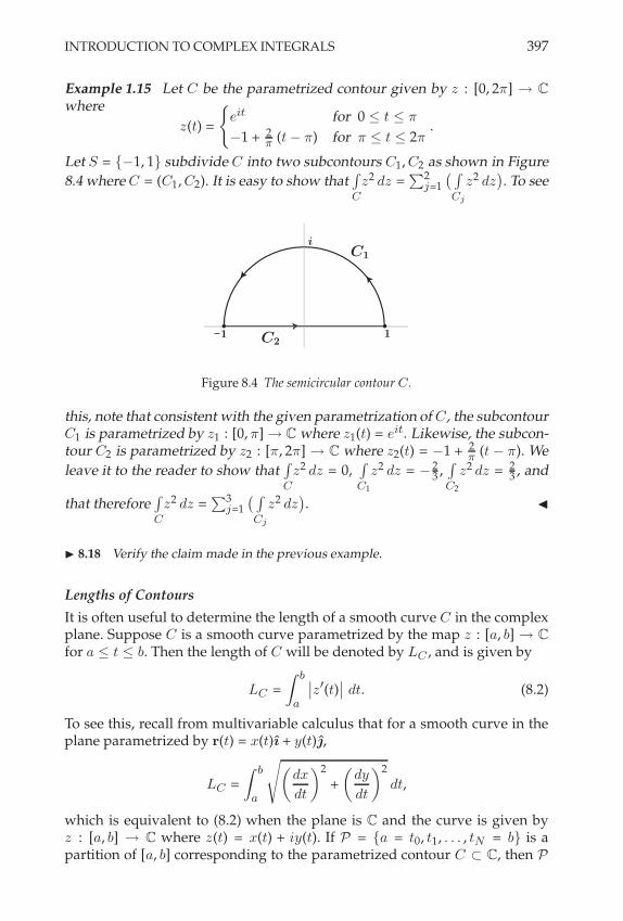
INTRODUCTION TO COMPLEX INTEGRALS 397
Example 1.15 Let C be the parametrized contour given by z : [0, 2%] 3 C
where
z(t) =
Eeit for 0 + t + %
"1 + 2$ (t " %) for % + t + 2%
.
Let S = {"1, 1} subdivide C into two subcontours C1, C2 as shown in Figure8.4 where C = (C1, C2). It is easy to show that
Z
C
z2 dz =;2
j=1
, Z
Cj
z2 dz-. To see
11
iC1
C2
Figure 8.4 The semicircular contour C.
this, note that consistent with the given parametrization of C, the subcontourC1 is parametrized by z1 : [0, %] 3 C where z1(t) = eit. Likewise, the subcon-tour C2 is parametrized by z2 : [%, 2%] 3 C where z2(t) = "1 + 2
$ (t " %). Weleave it to the reader to show that
Z
C
z2 dz = 0,Z
C1
z2 dz = "23 ,
Z
C2
z2 dz = 23 , and
that thereforeZ
C
z2 dz =;3
j=1
, Z
Cj
z2 dz-. "
! 8.18 Verify the claim made in the previous example.
Lengths of Contours
It is often useful to determine the length of a smooth curve C in the complexplane. Suppose C is a smooth curve parametrized by the map z : [a, b] 3 C
for a + t + b. Then the length of C will be denoted by LC , and is given by
LC =
Y b
a
&&z&(t)&& dt. (8.2)
To see this, recall from multivariable calculus that for a smooth curve in theplane parametrized by r(t) = x(t)ı + y(t)&,
LC =
Y b
a
F2dx
dt
32
+
2dy
dt
32
dt,
which is equivalent to (8.2) when the plane is C and the curve is given byz : [a, b] 3 C where z(t) = x(t) + iy(t). If P = {a = t0, t1, . . . , tN = b} is apartition of [a, b] corresponding to the parametrized contour C ' C, then P

398 COMPLEX INTEGRATION
subdivides C into subcontours C1, C2, . . . , CN , and
LC =N+
j=1
LCj .
! 8.19 Prove the above claim.
! 8.20 Consider C parametrized by z : (0, 1] , C where z(t) = t + i sin, 1
t
-. Find
LC . Is C a contour according to Definition 4.12 in Chapter 7? Why or why not?
The following result is the complex analog to Corollary 2.12 in Chapter 7.
Proposition 1.16 Suppose C is a parametrized contour contained in the open setD ' C, and that f : D 3 C is continuous on D. If " / max
z#C|f (z)|, then
&&&&
Y
C
f (z) dz
&&&& + " LC .
! 8.21 Prove the above proposition. Clearly it also holds if " is replaced by anyM > ".
Just as in the real line integral case, it is an extremely useful fact that if twoequivalent parametrizations of C ' C are given, the value of the integralof a complex function f along C will be the same with respect to either ofthe equivalent parametrizations used to describe C. We state this result moreformally in the following theorem, the proof of which is left to the reader.
Proposition 1.17 Suppose f : D 3 C is continuous on the open set D ' C, andC is a contour in D with parametrization z : [a, b] 3 D. Suppose Gz : [c, d] 3 D isa parametrization of C equivalent to z. Then,
Y
C
f (z) dz /
Y b
af (z(t)) z&(t) dt =
Y d
cf (Gz(s)) Gz&(s) ds.
! 8.22 Prove the above proposition. Refer to Proposition 1.3 on page 389.
Example 1.18 Consider the segment [1, i] and the integralZ
[1,i]
z dz. With the
standard parametrization z1 : [0, 1] 3 C given by z1(t) = 1 + t (i" 1), we haveY
[1,i]
z dz =
Y 1
0
,1 + t ("i " 1)
-(i " 1) dt = 2 + i.
With the equivalent parametrization z2 : ["1, 1] 3 C given by z2(t) = 1 +

INTRODUCTION TO COMPLEX INTEGRALS 399
12 (t + 1) (i " 1), we have
Y
[1,i]
z dz =
Y 1
"1
(1 + 1
2 (t + 1) ("i" 1))
12 (i " 1) dt = 2 + i,
and the integral has the same value for both parametrizations. "
Based on our results for contours in R2, for any contour C ' C withparametrization zC : [a, b] 3 C, the associated parametrized curve or con-tour "C consisting of the same set of points in C but traversed in the oppositeway can be parametrized by z"C : ["b,"a] 3 C where z"C (t) = zC ("t). Weleave it to the reader to show that if f : D 3 C is continuous in the open setD, and if C is a parametrized contour in D, then
Y
"C
f (z) dz = "
Y
C
f (z) dz.
! 8.23 Prove the above claim.
Example 1.19 Suppose C is a simple closed contour contained in an openset D ' C. Connect two points of C by a contour S ' D that passes onlythrough the interior of C. More specifically, consider Figure 8.5 with CL thecontour parametrized so as to be traversed from z1 to z3 via z2, and with CR
the contour parametrized so as to be traversed from z3 to z1 via z4. Take the
z2
z1
z3
z4
Sz5
CR
CL
Figure 8.5 The situation in Example 1.19.
closed contour C to be (CL, CR), and let S be the contour parametrized fromz3 to z1 via z5. Then note that for any function f : D 3 C that is continuouson (C % S) ' D, we have
\
Cf (z) dz =
\
CL
f (z) dz +
\
CR
f (z) dz
=
\
CL
f (z) dz +
Y
S
f (z) dz "
Y
S
f (z) dz +
\
CR
f (z) dz

400 COMPLEX INTEGRATION
=
\
(CL ,S)
f (z) dz +
\
(CR ,"S)
f (z) dz.
That is, the integral of f around the the closed contour C is equal to the sumof the integrals of f around the two closed contours (CL, S) and (CR,"S),and so we may interpret the integral of f along S and "S as “canceling eachother out.“ "
! 8.24 In the above example, suppose S connects two points of C by going throughthe exterior of C. Does the conclusion of the example still hold? That is, does theintegral of f along S still cancel out the integral of f along &S?
! 8.25 In the above example, suppose the contour C is not simple and S is a contourthat connects two points of C. Does the conclusion of the example still hold now?
! 8.26 Suppose C ! C is a closed contour parametrized by z : [a, b] , C. For anyt0 " R show that if C is reparametrized by Gz : [a+t0, b+t0] , C where Gz(t) . z(t&t0),then the value of
]
C
f (z) dz is unchanged.
2 FURTHER DEVELOPMENT OF COMPLEX LINE
INTEGRALS
2.1 The Triangle Lemma
One of the most important concepts in the theory of complex integrationis that, under the right conditions, the integral of a differentiable complexfunction around a closed contour is zero. We establish our first such resultnext. It will be critical to our development of what follows.
Lemma 2.1 (The Triangle Lemma)Suppose f : D 3 C is differentiable on the open set D ' C, and suppose theparametrized triangle = = [z0, z1, z2, z0] and its interior are contained in D. Then
\
/
f (z) dz = 0.
PROOF Let P0 be the perimeter of =, and let L0 be the length of the longestside of =. Let M1 be the midpoint of [z0, z1], let M2 be the midpoint of[z1, z2], and let M3 be the midpoint of [z2, z0]. Connect these midpoints toform four parametrized triangles T1 = [z0, M1, M3, z0], T2 = [M1, z1, M2, M1],T3 = [M2, z2, M3, M2], and T4 = [M3, M1, M2, M3], as shown below. As inExample 1.19 on page 399, it is easy to see that by cancelation of contourcontributions,\
/
f (z) dz =
\
T1
f (z) dz +
\
T2
f (z) dz +
\
T3
f (z) dz +
\
T4
f (z) dz.

FURTHER DEVELOPMENT OF COMPLEX LINE INTEGRALS 401
z0
z2
z1
#1
#2
#3
M1
M2
M3
Figure 8.6 Demonstration of the proof of the triangle lemma.
One of the smaller triangles T1, T2, T3, or T4, hereafter denoted by =1, has theproperty that &&&&
\
/
f (z) dz
&&&& + 4
&&&&
\
/1
f (z) dz
&&&&. (8.3)
(Why?) Consider the same procedure with =1 as the initial triangle (shadedin Figure 8.6), and of the four smaller triangles coming from =1, let the trian-gle having property (8.3) be denoted by =2. Then we have
&&&&
\
/
f (z) dz
&&&& + 4
&&&&
\
/1
f (z) dz
&&&& + 42
&&&&
\
/2
f (z) dz
&&&&.
Continuing this procedure indefinitely, we generate a sequence of triangles=,=1,=2, . . . such that
1.
&&&&]
/f (z) dz
&&&& + 4n
&&&&]
/n
f (z) dz
&&&&,
2. Pn = (perimeter of =n) = 12n P0,
3. Ln = (length of the longest side of =n) = 12n L0.
Now denote the closure of the interior of each triangle in this sequence by $
and by $j for j = 1, 2, . . . . Then, $ 9 $1 9 $2 9 · · · , forms a nested sequenceof closed sets, and therefore by Theorem 4.9 in Chapter 2 there exists a uniquez0 # $ &
,>'j=1 $j
-. Since f is differentiable at z0, for any ! > 0 there exists
. > 0 such that
0 < |z " z0| < . )
&&&&f (z) " f (z0)
z " z0" f &(z0)
&&&& <!
2 L0 P0.

402 COMPLEX INTEGRATION
Now choose N large enough that $N ' N+(z0). Then it follows that&&f (z) " f (z0) " f &(z0) (z " z0)
&& +!
2 L0 P0|z " z0|
+
!
2 L0 P0LN for all z # $N .
From this last inequality we obtain&&&&
\
/N
,f (z) " f (z0) " f &(z0) (z " z0)
-dz
&&&& +!
2 L0 P0LN PN =
!
2 (4N ). (8.4)
We leave it to the reader to show that]
/N
f (z0) dz =]
/N
f &(z0) (z " z0) dz = 0,
and therefore that]
/N
f (z) dz =]
/N
,f (z) " f (z0) " f &(z0) (z " z0)
-dz. This in
turn, along with (8.4), leads to&&&&
\
/
f (z) dz
&&&& + 4N
&&&&
\
/N
f (z) dz
&&&&
= 4N
&&&&
\
/N
,f (z) " f (z0) " f &(z0) (z " z0)
-dz
&&&&
+(2 < !,
and so,]
/f (z) dz = 0. #
! 8.27 Show that]
*N
f (z0) dz =]
*N
f#(z0) (z & z0) dz = 0 by parametrizing 5N and
computing.
The above result can clearly be applied to integrals along nontriangular con-tours, as the following example illustrates.
Example 2.2 Suppose f : D 3 C is differentiable on D and that the parametrizedrectangle R = [z0, z1, z2, z3, z0] and its interior is contained in D. Clearly Rcan be carved up into parametrized triangular pieces =1 and =2 such that]
R
f (z) dz =]
/1
f (z) dz +]
/2
f (z) dz. Since the integral over each triangle is zero,
it follows that]
R
f (z) dz = 0. "
! 8.28 Fill in the details of the above example.
An important refinement of the triangle lemma follows next. It says that thedifferentiability of f is allowed to be relaxed at a single point p # D, and yetthe result still holds.

FURTHER DEVELOPMENT OF COMPLEX LINE INTEGRALS 403
Corollary 2.3 Suppose f : D 3 C is continuous on D, and suppose the parametrizedtriangle = = [z0, z1, z2, z0] and its interior are contained in D. Assume that f is dif-ferentiable on D \ {p} for some p # D. Then
\
/
f (z) dz = 0.
PROOF 1 Note that if p is outside the triangle, the proof is the same as for theprevious theorem. There are three other cases to consider (see Figure 8.7).
a
b
p
cd
a
b
p
c
a
bp
c
Figure 8.7 Demonstration of the proof of Corollary 2.3 in Cases 1–3, from left to right.
Case 1: p is a vertex of =.
Denote the other two vertices of = by a and b, and let ! > 0 be given. Let" / max |f (z)|, the maximum value of f on (and within) =. Consider thefigure above, where we choose points c and d on = so that the perimeter ofthe triangle formed by c, d, and p, denoted by P/cdp
, is less than ("
. Then wehave \
/
f (z) dz =
\
[a,d,c,a]
f (z) dz +
\
[a,b,d,a]
f (z) dz +
\
[c,d,p,c]
f (z) dz
= 0 + 0 +
\
[c,d,p,c]
f (z) dz,
and so, &&&&
\
/
f (z) dz
&&&& =
&&&&
\
[c,d,p,c]
f (z) dz
&&&& + " P/cdp< !,
which yields the result.
Case 2: p lies on a side of =, but not on a vertex.
1We follow [Rud87] in the proof.

404 COMPLEX INTEGRATION
Denote the vertices of = by a, b, and c. Then,\
/
f (z) dz =
\
[a,b,p,a]
f (z) dz +
\
[a,p,c,a]
f (z) dz = 0 + 0 = 0.
Case 3: p lies in the interior of =.
Again, denote the vertices of = by a, b, and c. Then,\
/
f (z) dz =
\
[a,b,p,a]
f (z) dz +
\
[b,c,p,b]
f (z) dz +
\
[a,p,c,a]
f (z) dz = 0 + 0 + 0 = 0.
#
! 8.29 In the above proof, where in cases 2 and 3 is the result of case 1 implicitlyused? Extend the corollary to the case where f : D , C is differentiable on D \{p1, p2, . . . , pn} for p1, p2, . . . , pn " D.
2.2 Winding Numbers
To motivate what follows, consider the integral 12$i
]
C
dzz for some parametrized
closed curve C in C where 0 $# C. Since 0 $# C, we may parametrize C ac-cording to z(t) = r(t)ei"(t) where r(t) and $(t) are continuously differentiablefunctions on [a, b]. Following our noses in a nonrigorous way, we obtain
1
2% i
\
C
dz
z=
1
2% i
Y b
a
z&(t)
z(t)dt
=1
2% i
Y b
a
,r&(t) + i r(t)$&(t)
-ei"(t)
r(t)ei"(t)dt
=1
2% i
Y b
a
(r&(t)
r(t)+ i $&(t)
)dt
=1
2% i
2ln |r(t)|
&&&b
a+ i $(t)
&&&b
a
3
=$(b) " $(a)
2%
=#$
2%.
Here, #$ is the net change in the argument of z(t) as C is traversed oncefrom t = a to t = b. As we rigorously show in Appendix A, the value of #$
is an integer (not necessarily zero!) multiple of 2%. Hence, 12$ i
]
C
dzz can be
thought of as the number of times the contour C “winds around“ the origin.The definition below exploits this conclusion and characterizes a topologicalconcept that will be of surprisingly great use to us. In fact, the statements andproofs of many of our most potent results will rely on it.
FURTHER DEVELOPMENT OF COMPLEX LINE INTEGRALS 405
Definition 2.4 Let C be a closed parametrized contour in C, and considerany z0 $# C. The winding number of C about z0, denoted by nC (z0), is givenby
nC (z0) /1
2 % i
\
C
d0
0 " z0.
As described above, the number nC (z0) can be seen to be the number of timesthe contour C “winds around“ the point z0. A rigorous justification for thisgeometric interpretation can be found in Appendix A. To illustrate this ge-ometric connection to the formula in the above definition, we consider thesimple case where C = Cr(z0) is a circle of radius r centered at z0.
Example 2.5 Consider the circle C = Cr(z0) centered at z0 in the complexplane and parametrized by 0 : [0, 2 %] 3 C where 0(t) = z0 + r ei t. Then,
nC (z0) =1
2 % i
\
C
d0
0 " z0=
1
2 % i
Y 2 $
0
i r ei t dt
r ei t= 1.
"
! 8.30 Show that if you traverse the circle in the above example in the same coun-terclockwise direction, but n times rather than once, then nC (z0) = n. (Hint: What isthe parametrization for this new curve?)
! 8.31 Parametrize the circle from the above example in the opposite direction andshow that nC (z0) = &1.
Proposition 2.6 nC (z0) is an integer.
PROOF We prove the case where C is a smooth closed curve, and leave themore general case where C is a contour to the exercises. For C parametrizedby z : [a, b] 3 C, let F : [a, b] 3 C be defined by
F (s) /
Y s
a
z&(t)
z(t) " z0dt for s # [a, b].
Note that F (b) = 2 % i nC(z0). Also, by Proposition 1.4 on page 389 we have
F &(s) = z!(s)z(s)"z0
. Now consider the following derivative,
d
ds
MeF (s)
z(s) " z0
N
=
,z(s) " z0
-eF (s) F &(s) " eF (s) z&(s),z(s) " z0
-2= 0.
This yields that eF (s)
z(s)"z0is a constant for all s # [a, b], and therefore in partic-
ular,eF (a)
z(a) " z0=
eF (b)
z(b) " z0.
Since C is closed we have that z(a) = z(b), and so eF (a) = eF (b). This last

406 COMPLEX INTEGRATION
equality implies that F (b) = F (a)+2 % i m for some integer m. But since F (a) =0, we obtain
nC (z0) =F (b)
2 % i=
2 % i m
2 % i= m,
proving the result. #
! 8.32 Prove the above proposition for a general closed contour C.
For a fixed closed parametrized contour C ' C, we can allow the point z0 $#
C to vary continuously, thereby denoting it by z, and investigate how thevalue of nC (z) varies as a consequence. In light of this, for a fixed closedparametrized contour C in C, we may view nC : C \ C 3 Z as a function,given by
nC (z) /1
2 % i
\
C
d0
0 " z.
We will now try to characterize what integer values nC (z) may take, and hownC (z) may vary as z is varied for a given closed parametrized contour C.
Proposition 2.7 Let C be a closed parametrized contour in C. Then nC (z) is con-stant (and therefore a single integer value) on any connected subset of C \ C.
! 8.33 Prove the above theorem by establishing the following:
a) Show that nC is continuous on C \ C.
b) Show that if A ! C \ C is connected, then nC (A) must also be connected.
Proposition 2.8 Let C be a closed parametrized contour in C. Then nC (z) = 0 onany unbounded connected set in C \ C.
PROOF We handle the case where C is a smooth curve and leave the proofof the more general case where C is a contour to the reader. To this end, letA be an unbounded connected set in C \ C. Let z0 # A be far enough from Csuch that |z0 " 0(t)| ! LC for all t # [a, b]. Then
|nC (z0)| =1
2%
&&&&
\
C
d0
0 " z0
&&&&.
Since |0(t) " z0| ! LC , it follows that
|nC (z0)| +1
2% LCLC < 1,
which implies that nC (z0) = 0. (Why?) Finally, since A is connected, it followsfrom the previous proposition that nC (z) = 0 for all z # A. #
! 8.34 Answer the (Why?) question in the above proof, and complete the proof byestablishing the result for the case where C is a closed parametrized contour.

FURTHER DEVELOPMENT OF COMPLEX LINE INTEGRALS 407
! 8.35 In Example 2.5 on page 405, we found that the winding number nC (z0) fora counterclockwise circle C around its center z0 was 1. Consider this same contouragain. Let a be any point from Int(C). Show that nC (a) = 1. What if a " Ext(C)?
Example 2.9 Let R be a rectangle that is parametrized counterclockwise,and let z0 # Int(R). We will show that nR(z0) = 1 using a technique some-times referred to as “the horseshoe method.“ Without any loss of generality,let z0 be the origin of the complex plane, and choose Cr ' Int(R) whereCr / Cr(0) is the parametrized circle of radius r centered at 0. Considerthe simple closed contours C1 and C2 as shown in Figure 8.8. (C1 has initialpoint z1, and passes through z2, z3, z4, z5, z6, and z7 as t increases, terminat-ing at z1. Likewise, C2 starts at z1 and passes through z8, z6, z5, z9, z10, andz2 before terminating at z1.) Clearly, 0 # Ext(C1) and 0 # Ext(C2), and so
z1
z0
z2
z4
z3
z5
z6
z7 z8
z9
z10
C1
C2
Cr
Figure 8.8 The horseshoe method of computing the winding number of a rectangular contour.Note the shading of the interiors of C1 and C2.
nC1(0) = nC2
(0) = 0. But since
0 = nC1(0) + nC2
(0)
=1
2% i
\
C1
dz
z+
1
2% i
\
C2
dz
z
=1
2% i
\
R
dz
z"
1
2% i
\
Cr
dz
z(Why?)
= nR(0) " nCr (0),
it follows that nR(0) = nCr (0). Since nCr (0) = 1, we have that nR(0) = 1. "
! 8.36 Answer the (Why?) question in the above example. See Example 1.19 on page399 for a clue.

408 COMPLEX INTEGRATION
2.3 Antiderivatives and Path-Independence
An antiderivative associated with a complex function f is defined as in thereal function case. That is, for open D ' C, consider f : D 3 C and sup-pose there exists a differentiable function F : D 3 C such that F &(z) = f (z)for all z # D. Then F is called an antiderivative of f on D. As you might ex-pect, antiderivatives play a useful role in evaluating line integrals of complexfunctions.
Proposition 2.10 (The Fundamental Theorem of Calculus)Suppose f : D 3 C is continuous on the open set D ' C and let C be a parametrizedcontour in D with initial and terminal points zI and zT , respectively. If f has anantiderivative F on D, then
Y
C
f (z) dz = F (zT ) " F (zI ).
! 8.37 Prove the above proposition.
In practice, the contour C referred to in Proposition 2.10 will have a particularparametrization z : [a, b] 3 C with zI = z(a) and zT = z(b). However, itshould be clear that the choice of parametrization does not matter, since thevalue of the integral does not depend on it. This is a very practical theorem. Itsays that when you know an antiderivative for f , you can evaluate
Z
C
f (z) dz
without applying Definition 1.11, and the result depends only on the initialand terminal points of C. The following corollary, partly illustrated in Figure8.9, is a useful consequence of Proposition 2.10.
Corollary 2.11 Suppose f : D 3 C is continuous on the open set D ' C and hasantiderivative F there.
a) If C is a closed parametrized contour in D, then]
C
f (z) dz = 0.
b) Let z1 and z2 be any two points in D. If C1 and C2 are any two parametrizedcontours in D with initial point z1 and terminal point z2, then
Y
C1
f (z) dz =
Y
C2
f (z) dz.
! 8.38 Prove the above corollary.
! 8.39 If Gz is another parametrization for C, is the result of part a) of the abovecorollary still true? Does it matter if Gz is equivalent to z or not? Does the result of partb) depend on the parametrizations used for C1 and C2?

FURTHER DEVELOPMENT OF COMPLEX LINE INTEGRALS 409
C1
C2
z1
z2
Figure 8.9 The situation in Corollary 2.11, part b): path independence.
Corollary 2.11 tells us that the class of complex functions that are continuousand have an antiderivative on D is an especially nice class. If f : D 3 C
is such a function, then not only can we conclude that]
C
f (z) dz = 0 for any
closed contour C ' D, we can also conclude that the integral of f from onepoint to another in D is path independent. That is, the value of the integraldepends only on the initial point and the terminal point, not on the path(within D) taken between them. This is significant. After all, in general forf : D 3 C there are infinitely many paths within D that connect two points inD. The answer to the question When will the integral of a complex function f fromone point to another not depend on the choice of contour between them? is importantfor both practical and theoretical reasons. In particular, the property of pathindependence is convenient, since it allows one to choose a different contourthan the one specified (if specified) connecting the initial point to the terminalpoint.
Example 2.12 We will evaluate the integralZ
C
ez dz where C is the curve
parametrized by z : [0, 2%] 3 C where z(t) = t + i sin t. Note that sincef (z) = ez has antiderivative F (z) = ez on C, we may change the path C to GCparametrized by Gz : [0, 2%] 3 C where Gz(t) = t. Then we have
Y
C
ez dz =
Y
GC
eGz dGz =
Y 2$
0et dt = e2$
" 1.
"
The results indicated in Corollary 2.11 need deeper exploration. In particu-lar, we would like to identify exactly those properties a function f , a set D,and a closed contour C need to possess so that f has an antiderivative in D.More generally, we would like to identify the properties f , D, and the closed

410 COMPLEX INTEGRATION
contour C need to possess so that]
C
f (z) dz = 0. There are many technical
hurdles to overcome in handling this topic properly, and so we will moveforward carefully. The geometry/topology of the set D in which our func-tion is defined will become more significant as we continue to “fine-tune“the statements of our theorems. In light of this, the following concept will beespecially useful.
2.4 Integration in Star-Shaped SetsStar-Shaped Sets
We begin with a definition.
Definition 2.13 A set D ' C is star-shaped if there exists z0 # D such that[z0, z] ' D for every z # D. Such a point z0 # D is sometimes called a starcenter.
Figure 8.10 provides examples of star-shaped sets and a set that is not star-shaped.
Figure 8.10 Two star-shaped sets (to the left) with star centers shown, and one set that is notstar-shaped (to the right).
A special subclass of star-shaped sets, and one that is probably more familiar,is the class of convex sets. A set is convex if the line segment connecting anypair of points of the set is completely contained in the set. A star-shaped set isone that contains at least one star center. A convex set is one for which everypoint is a star center. Simple examples of convex sets, and therefore star-shaped sets, are disks, rectangles, and ellipses. The following, nonconvex setis star-shaped. Consider a point z) # C, and let R be any ray beginning at z).Then D / C \ R is star-shaped, but not convex.
! 8.40 Let D ! C be star-shaped and suppose f : D , C is such that f# . 0 on D.
Show that f . c on D for some c " C.
The star-shaped condition on D allows us to rephrase one of our earlier re-sults. Recall that Corollary 2.11 on page 408 stated that if the continuous func-

FURTHER DEVELOPMENT OF COMPLEX LINE INTEGRALS 411
tion f : D 3 C had an antiderivative on the open set D ' C, then the integralof f around any closed contour contained in D is zero and the integral of fbetween any two points z1, z2 # D is path independent. For the function f ,the key to the path-independence property holding is the existence of an an-tiderivative for f on D. The following result establishes convenient sufficientconditions for the existence of such an antiderivative in the case where theopen set D is star-shaped.
Theorem 2.14 Suppose f : D 3 C is differentiable on the open star-shaped setD ' C. Then f has an antiderivative on D.
Of course, the significant consequences of having an antiderivative on D areprecisely those listed in the conclusion of Corollary 2.11, namely, if z1 andz2 are any two points in D, then the integral of f within D along contoursstarting from z1 and ending at z2 are path independent. Also, integrals of falong closed contours within D are zero.
PROOF Let z) # D be such that [z), z] ' D for all z # D, i.e., z) is a starcenter for D. We define F : D 3 C for the parametrized [z), z] by
F (z) /
Y
[z%,z]
f (0) d0.
We will show that for each z0 # D,
F &(z0) = limz(z0
F (z) " F (z0)
z " z0= f (z0).
To establish this, we note that since f is continuous at z0, given ! > 0 thereexists . > 0 such that
|0 " z0| < . ) |f (0) " f (z0)| < (2 .
Since we wish to consider points near z0 that are also elements of D, we take. small enough that N+(z0) is entirely contained in D. (See Figure 8.11.) For
z
z0
[z$, z0]
[z$, z]
N%(z0)z$
Figure 8.11 The situation in the proof of Theorem 2.14.
412 COMPLEX INTEGRATION
such a ., it follows that for z satisfying 0 < |z " z0| < . we have&&&&F (z) " F (z0)
z " z0" f (z0)
&&&& =
&&&&1
z " z0
Y
[z0,z]
f (0) d0 " f (z0)
&&&&
=
&&&&&1
z " z0
Y
[z0,z]
f (0) d0 "
1
z " z0
Y
[z0,z]
f (z0) d0
&&&&&
=1
z " z0
&&&&&
Y
[z0,z]
,f (0) " f (z0)
-d0
&&&&&
+
1
|z " z0|
(2 |z " z0|
= (2
< !, (8.5)
and therefore F is an antiderivative of f on D. By Corollary 2.11 on page 408integrals of f on contours C ' D are path independent. #
Note that in the above proof, the first equality in expression (8.5) implicitlymakes use of the identity
1
z " z0
C Y
[z%,z]
f (0) d0 "
Y
[z%,z0]
f (0) d0
D
=1
z " z0
C Y
[z0,z]
f (0) d0
D
. (8.6)
Here, the existence of the difference on the left-hand side requires that theintegrals along the parametrized segments [z), z] and [z), z0] be well defined,i.e., that these segments are contained in D. That D is star-shaped with starcenter z) ensures this. Equality (8.6) then follows from the triangle lemma.
The following corollary to the above theorem weakens the conditions on fjust a bit, and yet the conclusion still holds. This corollary will be neededwhen we prove the Cauchy integral theorem in the next section.
Corollary 2.15 Suppose f : D 3 C is differentiable on the open star-shaped setD ' C, except possibly at a single point p # D where f is merely continuous. Thenf still has an antiderivative on D.
! 8.41 Prove the above corollary.
The conclusion to the above corollary holds even if the number of excludedpoints p1, . . . , pn, is greater than one, but finite. We leave the proof of this tothe reader.
! 8.42 Prove that the conclusion to Corollary 2.15 still holds even for a finite collec-tion p1, . . . , pn of excluded points.

FURTHER DEVELOPMENT OF COMPLEX LINE INTEGRALS 413
z0
a
C1
Cs(z0)Cs(z0)
Cr(a)Cr(a)
z0 a
C2
R1
R2
Figure 8.12 The contours in the horseshoe construction of Example 2.16, with rays shown.
Example 2.16 Let Cr / Cr(a) and suppose z0 # C is such that |z0 " a| < r.We will show that
]
Cr
dzz"z0
= 2% i. To this end, choose s > 0 so that Cs /
Cs(z0) ' Int(Cr). Define the parametrized contours C1 and C2 as shown inFigure 8.12, and such that
\
C1
dz
z " z0+
\
C2
dz
z " z0=
\
Cr
dz
z " z0"
\
Cs
dz
z " z0.
In fact,]
Cj
dzz"z0
= 0 for j = 1, 2. To see this, embed C1 in a star-shaped region
D1 / C \R1, formed by omitting the ray R1 emanating from z0 from C. Nownote that 1
z"z0is differentiable on D1. Similarly, embed C2 in a star-shaped
region D2 / C \ R2 on which 1z"z0
is differentiable. Since]
Cs
dzz"z0
= 2% i, it
must also be true that]
Cr
dzz"z0
= 2% i. "
Example 2.17 Let D / C \ R where R = ("-, 0] is the ray from the originalong the negative real axis. Note that z) = 1 is a star center for D and soD is star-shaped. Since 1
z is differentiable on D, Theorem 2.14 implies thatthere exists a function F : D 3 C such that F is differentiable on D andF &(z) = 1
z . We will show that the function F is related to a branch of the
logarithm function. To see this, consider F : D 3 C given by F (z) /Z
[1,z]
d// .
Since F is differentiable on D, it follows that F = U + i V where -U-x = -V
-y ,
and -U-y = "
-V-x . We also have
F &(z) =*U
*x+ i
*V
*x=
1
z=
x
x2 + y2" i
y
x2 + y2,

414 COMPLEX INTEGRATION
and therefore,*U
*x=
x
x2 + y2and
*V
*x= "
y
x2 + y2. (8.7)
Integrating each equation in (8.7) with respect to x yields
U (x, y) = ln%
x2 + y2 + c1, and V (x, y) = tan"1 , yx
-+ c2,
where c1 and c2 are constants. From this, we have
F (z) = U + i V = ln%
x2 + y2 + i tan"1 , yx
-+ (c1 + i c2),
and since F (1) = 0, we see that c1 + i c2 / 0. Therefore,
F (z) = ln |z| + i Arg(z) / log(z),
for Arg(z) # ("%, %). Here, Arg : D 3 ["%, %) is a (nonprincipal) branchof the argument of z, and log(z) is its associated (nonprincipal) branch of thelogarithm function as described in Chapter 4. The function F is the restrictionof log(z) to D. "
! 8.43 Consider the situation described in the previous example, but with D . C\R
where R is some other ray emanating from z0 " C. How does the result differ in thiscase?
Example 2.18 Suppose D ' C is open and star-shaped, and f : D 3 C \
{0} is twice differentiable on D. We will show that f has a differentiablelogarithm on D, i.e., that there exists g : D 3 C such that g is differentiable
on D and eg(z) = f (z) on D. By Theorem 2.14, since f !(z)f (z) is differentiable on
D it must have an antiderivative F (z) on D, i.e., F &(z) = f !(z)f (z) . Now, since
,f (z) e"F (z)
-& = f &(z) e"F (z)" f (z) e"F (z) F &(z) = 0, it follows that there exists
some z0 # D such that f (z) e"F (z) = c = ez0 on D, and f (z) = eF (z)+z0 . Thefunction F (z) + z0 is sometimes called a differentiable logarithm of f . "
Example 2.19 Suppose D ' C is open and star-shaped and f : D 3 C \ {0}is twice differentiable on D. Suppose also that g is a differentiable logarithmof f on D. If C ' D is any contour parametrized by z : [a, b] 3 C, we will
show thatZ
C
f !(z)f (z) dz = g
,z(b)
-" g
,z(b)
-. To see this, note that f (z) = eg(z),
and so it follows that f &(z) = eg(z) g&(z), or g&(z) = f !(z)eg(z) = f !(z)
f (z) , i.e., g(z) is an
antiderivative of f !(z)f (z) . This implies that
Z
C
f !(z)f (z) dz = g
,z(b)
-" g
,z(a)
-. "
The following theorem establishes a useful equivalence that summarizes manyof the significant results of this section.

CAUCHY’S INTEGRAL THEOREM AND ITS CONSEQUENCES 415
Theorem 2.20 Suppose f : D 3 C is continuous on the open connected set D.Then the following are equivalent:
(i) Integrals of f in D are path independent.
(ii) Integrals of f around closed contours in D are 0.
(iii) There is an antiderivative F : D 3 C for f on D.
PROOF By Corollary 2.11 we see that (iii) ) (i), and that (iii) ) (ii). We leaveit to the reader to show that (i) 5 (ii). We now prove that (i) ) (iii). Fix a # D.Then, for any contour C ' D that has initial point a # D and terminal pointz # D, define F : D 3 C by
F (z) /
Y
C
f (0) d0.
We now show that F &(z0) = f (z0) for every point z0 # D. Note that forany contour C0 in D with initial point a and terminal point z0 there existsNr(z0) ' D, and for z # Nr(z0) we have that [z0, z] ' Nr(z0) ' D. (Why?)Therefore,
F (z) " F (z0) =
Y
C
f (0) d0 "
Y
C0
f (0) d0 =
Y
[z0,z]
f (0) d0.
This yields
F (z) " F (z0) " f (z0) (z " z0) =
Y
[z0,z]
,f (0) " f (z0)
-d0.
Since f is continuous, for each ! > 0 there exists . > 0 such that
|0 " z0| < . ) |f (0) " f (z0)| < !.
Choosing . < r, we obtain
|z " z0| < . ) |F (z) " F (z0) " f (z0) (z " z0)| + ! |z " z0|,
which implies F &(z0) = f (z0). #
! 8.44 Prove (i) 2 (ii) in the above theorem.
! 8.45 Show that connectedness is not necessary in the above theorem.
3 CAUCHY’S INTEGRAL THEOREM AND ITS
CONSEQUENCES
We will now generalize the triangle lemma to more general simple closedcontours in D. The resulting Cauchy’s integral theorem is as fundamentalto the theory of complex functions as the Cauchy-Riemann equations. Many

416 COMPLEX INTEGRATION
zj
zj
Nr(zj!1)
zj!1
zj!1
PjCj
Figure 8.13 The proof of Lemma 3.1.
far-reaching results are a consequence of it, which we will see in a later sec-tion of this chapter. For now, it can be seen as a generalization of the circum-stances under which differentiable functions f : D 3 C that don’t necessar-ily have an antiderivative on D still satisfy
]
C
f (z) dz = 0 for closed contours
C ' D.
3.1 Auxiliary Results
In order to prove Cauchy’s integral theorem we will need several technicalresults. In the first of these we establish that for any function f : D 3 C thatis differentiable on the open set D, and any parametrized contour C ' D,the integral of f along C is equal to the integral of f along a rectangularparametrized contour P ' D consisting of only vertical and horizontal seg-ments.
Lemma 3.1 Let C be a contour in the open set D ' C, and let C be parametrizedby zC : [a, b] 3 C. Then there exists a rectangular contour P in D with parametriza-tion zP : [a, b] 3 C satisfying zP (a) = zC (a) and zP (b) = zC (b) such that iff : D 3 C is any differentiable function on D,
Y
C
f (z) dz =
Y
P
f (z) dz.
PROOF Choose r > 0 small enough so that |zC (t) " w| ! r for all w # DC
and for all t # [a, b]. Since zC(t) is continuous on the closed interval [a, b], it is

CAUCHY’S INTEGRAL THEOREM AND ITS CONSEQUENCES 417
uniformly continuous there, and so there exists . > 0 such that for t, s # [a, b],
|t " s| < . ) |zC (t) " zC (s)| < r,
and this . is independent of t and s. Now, choose a partition P = {a =t0, t1, . . . , tN = b} of [a, b] with 2P2 < . and such that zC (tj"1) $= zC(tj) for1 + j + N . Also, for notational convenience, let zj / zC (tj) for 0 + j + N .If Cj is the smooth piece of C parametrized by zCj
: [tj"1, tj] 3 C wherezCj
(t) / zC (t) for t # [tj"1, tj], then it follows that |zCj(t) " zj"1| < r for
t # [tj"1, tj], i.e., Cj ' Nr,zj"1
-for j = 1, 2, . . . , N . By our choice of r we
have that Nr,zj"1
-' D for j = 1, 2, . . . , N . Now, since each Nr
,zj"1
-is star-
shaped, we can replace Cj by a rectangular contour Pj having parametriza-tion zPj : [tj"1, tj] 3 C that lies in Nr
,zj"1
-and that connects zj"1 to zj (see
Figure 8.13). By Corollary 2.11 on page 408 and Theorem 2.14 on page 411,we know that
Z
Cj
f (z) dz =Z
Pj
f (z) dz. Let P / (P1, P2, . . . , PN ). Then P is rect-
angular, and part b) of Proposition 1.14 on page 396 yieldsY
C
f (z) dz =
Y
P
f (z) dz. #
Clearly the above lemma holds for both open and closed contours C.
Now that we have established that integrals along contours can be adequatelyreplaced by integrals along rectangular contours, we state and prove a keylemma relating to integrals along rectangular contours.
Lemma 3.2 Suppose P is a closed rectangular parametrized contour in C. Thenthere exist counterclockwise-parametrized rectangles R1, . . . , RN in C such that for
arbitrary points wj # Int(Rj) for 1 + j + N , and for g :#N
j=1 Rj 3 C continuous
on#N
j=1 Rj , \
P
g(z) dz =N+
j=1
2nP (wj)
\
Rj
g(z) dz
3.
PROOF 2 Let P = [z0, z1, . . . zM"1, zM , z0] for some M # N. We begin bychoosing a rectangle R ' C that contains all of P in its interior. Form agrid of rectangles Rj for 1 + j + N by extending each segment of P in
both directions until it intersects R. Note that P '
#Nj=1 Rj , where each Rj is
parametrized counterclockwise. For each Rj let wj be an arbitrary point from
Int(Rj). Note that#N
j=1 Rj consists of parametrized segments of two types,each of which is a parametrized side of some rectangle Rj . A segment of the
2The proof of this technical lemma, and this approach to Cauchy’s integral theorem, aretaken from [AN07].

418 COMPLEX INTEGRATION
R
P
&
'
Figure 8.14 The proof of Lemma 3.2, with a sigma (-) and a tau (2 ) segment shown.
first type, hereafter referred to as a tau segment, is not a segment of P . A seg-ment of the second type, hereafter referred to as a sigma segment, is a segmentof P . We will show that
\
P
g(z) dz =N+
j=1
2nP (wj )
\
Rj
g(z) dz
3(8.8)
for any function g :#N
j=1 Rj 3 C that is continuous on#N
j=1 Rj . To do this,we will prove that the parametrized tau segments make no net contributionto the right-hand side of equality (8.8), and that each parametrized sigmasegment, 1 =
,P & Rj
-for some j, contributes an equal amount to each side
of equality (8.8). The situation is illustrated in Figure 8.14.
Let / be a parametrized tau segment of rectangle RI where / is not containedin P . We will show that / makes no net contribution to the right-hand side of(8.8). There are two cases to consider, each illustrated in Figure 8.15:
RI
RJ
RI
Case 2Case 1
&
&
Figure 8.15 The two cases in the proof for 2 segments.
Case 1: / is a common side for adjacent rectangles RI and RJ , i.e., / is notpart of R.
Since / is not contained in P , it follows that the segment [wI , wJ ] does notintersect P , and therefore
nP (wI ) = nP (wJ ). (Why?)

CAUCHY’S INTEGRAL THEOREM AND ITS CONSEQUENCES 419
The only contributions from / to the right-hand side of (8.8) are from theterms
nP (wI )
\
RI
g(z) dz + nP (wJ )
\
RJ
g(z) dz,
whose / -related contributions are, more explicitly,
nP (wI )
Y
0
g(z) dz + nP (wJ )
Y
"0
g(z) dz =,nP (wI ) " nP (wJ )
- Y
0
g(z) dz = 0.
Case 2: / is a side of exactly one rectangle RI , i.e., / is part of R.
In this case, since / is not contained in P it follows that nP (wI ) = 0. Tosee this, note that / is part of R but not a part of P . Therefore, there ex-ists a ray from wI that crosses / and therefore exits Int(R) but never in-tersects P . Proposition 2.8 on page 406 then yields that nP (wI ) = 0, andhence the only contribution from / to the right-hand side of equation (8.8)is nP (wI )
Z
0g(z) dz = 0.
Now suppose,P & RI
-$= ! for some I . Then
,P & RI
-consists of one or
more segments. Fix one. It must be a common side of two adjacent rectan-gles, RI and RJ . Parametrize the segment from one endpoint to the other (itwill not matter which endpoint is considered the initial point and which theterminal point) and denote the parametrized segment by 1. We will showthat the contribution of 1 to each side of equality (8.8) is the same. Begin byconsidering the left-hand side of (8.8), and let ' ! 0 be the number of timesthe parametrized segment 1 is traversed in a single traversal of P . Similarly,let ( ! 0 be the number of times the parametrized segment "1 is traversedin a single traversal of P (see Figure 8.16). Then the net contribution of 1 to
(
')
Figure 8.16 The meaning of the quantities ! and ".
]
P
g(z) dz is ('"()Z
1g(z) dz. We will now show that the parametrized segment
1 contributes the same amount, (' " ()Z
1g(z) dz, to the right side of (8.8). To
see this, we note that the only place the termZ
1g(z) dz can appear in the right
side of (8.8) is in
nP (wI )
\
RI
g(z) dz + nP (wJ )
\
RJ
g(z) dz. (8.9)

420 COMPLEX INTEGRATION
The 1 contributions to (8.9) are given by
nP (wI )
Y
1
g(z) dz + nP (wJ )
Y
"1
g(z) dz =,nP (wI ) " nP (wJ )
-Y
1
g(z) dz.
We will show that,nP (wI ) " nP (wJ )
-= (' " (), which will complete the
proof. To show this, consider\
P
g(z) dz " (' " ()
\
RI
g(z) dz =
\
GP
g(z) dz. (8.10)
Here, GP is the closed rectangular contour obtained by traversing P but de-touring around the 1 segment of RI along the other three sides of RI . Ob-
tained in this way, GP does not contain 1, and the points wI and wJ endup in the same unbounded connected region of the plane determined by
the closed contour GP (see Figure 8.17). Since 1 is not contained in GP , it fol-
P ˜P
wI wJwI
wJ
' '
Figure 8.17 An example of the replacement of P by P , where the whole grid of rectangles isnot shown in either case.
lows that n GP (wI ) = n GP (wJ ). Since equation (8.10) holds for any function
g :#N
j=1 Rj 3 C that is continuous on#N
j=1 Rj , we may choose g to be given
by g(z) = 1z"wI
. We may also choose g to be given by g(z) = 1z"wJ
. Makingthese substitutions into 8.10 and multiplying each integral in that equality by
12$i yields that
nP (wI ) " (' " () = n GP (wI ) = n GP (wJ ) = nP (wJ ),i.e.,
nP (wI ) " nP (wJ ) = ' " (.
This completes the proof. #
3.2 Cauchy’s Integral Theorem
The following result is the main result of this section and one of the keyresults of complex function theory. Its proof relies on Lemma 3.2.

CAUCHY’S INTEGRAL THEOREM AND ITS CONSEQUENCES 421
Theorem 3.3 (Cauchy’s Integral Theorem)Let C be a closed parametrized contour in the open set D ' C, and suppose nC (w) =0 for all w # DC . If f : D 3 C is differentiable on D, then
\
C
f (z) dz = 0.
PROOF 3 By Lemma 3.1, there exists a closed rectangular parametrized con-tour P in D (see Figure 8.18) such that for any g : D 3 C differentiable onD, \
C
g(z) dz =
\
P
g(z) dz.
If we choose g = f we obtain]
C
f (z) dz =]
P
f (z) dz, and if we choose g(z) = 1z"w
for w # DC it follows that
nP (w) = nC(w) = 0 for all w # DC .
Therefore, we need only establish the theorem for P . By Lemma 3.2, we canfind rectangles R1, . . . , RN in C and points wj # Int(Rj) for 1 + j + N suchthat \
P
g(z) dz =N+
j=1
2nP (wj )
\
Rj
g(z) dz
3
for all functions g continuous on#N
j=1 Rj . Let Sj / Int(Rj). Since f is differ-
R
PD
Figure 8.18 The proof of Cauchy’s integral theorem, with the points zj shown and the rect-angles contained in D shaded darker.
entiable on D, it must be continuous on P %
#
Sj0D
Sj . By the Tietze extension
3We follow [AN07] in the proof.

422 COMPLEX INTEGRATION
theorem, we may extend f to a continuous function Gf on all of C such thatGf = f on P %
#
Sj0D
Sj . Therefore,
\
P
Gf (z) dz =N+
j=1
2nP (wj)
\
Rj
Gf (z) dz
3. (8.11)
There are two cases to consider, Sj ' D and Sj $' D. If Sj ' D, then by the
triangle lemma]
Rj
Gf (z) dz =]
Rj
f (z) dz = 0. If Sj $' D, there exists w # Sj &DC
such that [wj , w] does not intersect P , and therefore
nP (wj ) = nP (w) = 0.
In either case we have nP (wj )]
Rj
Gf (z) dz = 0, and therefore,
\
P
f (z) dz =
\
P
Gf (z) dz =N+
j=1
2nP (wj)
\
Rj
Gf (z) dz
3= 0. #
Corollary 3.4 Let C be a simple closed parametrized contour in the open set D '
C such that Int(C) ' D. If f : D 3 C is differentiable on D, then\
C
f (z) dz = 0.
PROOF Consider any w # DC . Then w # Ext(C), and so nC (w) = 0. Theresult follows from the previous theorem. #
An example illustrates the power of Cauchy’s integral theorem.
Example 3.5 Suppose C is the contour shown in Figure 8.19 parametrizedby z : [0, 2%] 3 C where
z(t) =
Et + i sin t for 0 + t + %
2% " t for % < t + 2%.
It then follows from Cauchy’s integral theorem that]
C
ecos z dz = 0. "
The conclusion of the corollary to Cauchy’s integral theorem, namely, that]
C
f (z) dz = 0 for a simple closed contour C ' D such that Int(C) ' D, clearly
holds if f has an antiderivative F on D. From this we see that Cauchy’s in-tegral theorem gives more general conditions under which the integral of afunction f around a closed contour equals zero.

CAUCHY’S INTEGRAL THEOREM AND ITS CONSEQUENCES 423
C
0*
Figure 8.19 The contour of Example 3.5.
3.3 Deformation of Contours
The following results provide a convenient means for determining the valueof the integral of f : D 3 C along a closed contour C1 ' D by givingconditions under which C1 can be replaced by a simpler contour C2. Theeffect is that, under the right circumstances, one can think of “deforming“ thecontour C1 into the simpler contour C2, and thereby determine
]
C1
f (z) dz by
computing]
C2
f (z) dz instead. With experience, these results provide a useful
visual intuition for manipulating such integrals in C.
Theorem 3.6 Suppose D ' C is open and connected, and that f : D 3 C isdifferentiable on D.
a) Let C1 and C2 be closed parametrized contours in D such that for all w # DC
nC1(w) = nC2
(w). Then]
C1
f (z) dz =]
C2
f (z) dz.
b) Let {C, C1, C2, . . . , CN} be a collection of closed parametrized contours in
D, and suppose nC (w) =;N
j=1 nCj (w) for all w # DC . Then]
C
f (z) dz
=;N
j=1
]
Cj
f (z) dz.
PROOF We prove part a) and leave the proof of part b) to the reader. Let C1and C2 be parametrized by z1 : [a, b] 3 D and z2 : [c, d] 3 D, respectively.Figure 8.20 illustrates one possible situation. Since D is connected, we mayfind a contour C3 in D that is parametrized by z3 : [', (] 3 D such thatz3(') = z1(a) and z3(() = z2(c). Now let C = (C1, C3,"C2,"C3). Note that Cis closed and contained in D.
Let w # DC . Then w $# C ' D, and since\
C
dz
z " w=
\
C1
dz
z " w+
Y
C3
dz
z " w+
\
"C2
dz
z " w+
Y
"C3
dz
z " w,

424 COMPLEX INTEGRATION
C1
C2
Figure 8.20 The situation in case a) of Theorem 3.6.
we obtain after multiplying by 12$i ,
nC (w) = nC1(w) +
1
2 % i
Y
C3
dz
z " w" nC2
(w) "1
2 % i
Y
C3
dz
z " w= 0.
Therefore by Cauchy’s integral theorem, for any f : D 3 C where f is dif-ferentiable on D, we have that
]
C
f (z) dz = 0. Since for any such f we also
have\
C
f (z) dz =
\
C1
f (z) dz +
Y
C3
f (z) dz +
\
"C2
f (z) dz +
Y
"C3
f (z) dz
=
\
C1
f (z) dz "
\
C2
f (z) dz,
the result is proved. #
! 8.46 Prove part b) of the above theorem.
Example 3.7 Let C1 be the parametrized nonsimple closed contour indi-cated in Figure 8.21. By the geometric interpretation suggested in AppendixA, this contour has winding number +1 around the origin. Let C2 be theparametrized circle given by z2 : [0, 2%] 3 C where z2(t) = ei t. Then, ac-cording to Theorem 3.6, we have
]
C1
cos zz dz =
]
C2
cos zz dz. "
Example 3.8 Let z1 = 12 (% + i), z2 = 1
2 (3% " i), and consider the function f :
D 3 C given by f (z) = 1(z"z1) (z"z2) where D / C \ {z1, z2}. Let C = (C&, C')
where C& is the parametrized cycle of the sine curve given by z& : [0, 2%] 3 C
where z&(t) = (t, sin t), and C' is the parametrized segment of the real axisfrom 2 % to the origin given by z' : [2%, 4%] 3 C where z'(t) = (4% " t, 0).By the geometric interpretation suggested in Appendix A, the contour C haswinding number "1 around z1, and winding number +1 around z2. Let C1

CAUCHY’S INTEGRAL THEOREM AND ITS CONSEQUENCES 425
C1
C2
Figure 8.21 The nonsimple closed contour winding once around the origin in Example 3.7.
be a circle of small enough radius !1 > 0 centered at z1 and parametrizedclockwise, and let C2 be a circle of small enough radius !2 > 0 centered atz2 and parametrized counterclockwise. (See Figure 8.22.) By Theorem 3.6, we
C
C1
C2
Figure 8.22 The contours of Example 3.8.
see that \
C
dz
(z " z1) (z " z2)=
\
C1
dz
(z " z1) (z " z2)+
\
C2
dz
(z " z1) (z " z2).
"
Theorem 3.6 is a very useful result. The following corollaries make this plainer.The first is illustrated in Figure 8.23.
Corollary 3.9 Let f : D 3 C be differentiable on the open connected set D, andsuppose C1 and C2 are simple closed contours in D such that
(i) C2 ' Int(C1),
(ii) Ext(C2) & Int(C1) ' D,
(iii) nC2(z) = nC1
(z) for all z # Int(C2).
Then,

426 COMPLEX INTEGRATION
\
C1
f (z) dz =
\
C2
f (z) dz.
PROOF By Theorem 3.6 it suffices to show that nC2(w) = nC1
(w) for all w #
DC . From (ii),
DC'
,Ext(C2)
-C%
,Int(C1)
-C =,C2 % Int(C2)
-%
,C1 % Ext(C1)
-,
and since C1, C2 ' D, we have
DC' Int(C2) % Ext(C1),
where Int(C2) & Ext(C1) = !. Now suppose w0 # DC . Then there are two
C1 C2
Figure 8.23 The situation in Corollary 3.9.
cases, w0 # Int(C2) and w0 # Ext(C1). If w0 # Int(C2), then by condition (iii)nC2
(w0) = nC1(w0). For the case w0 # Ext(C1), we leave it to the reader to
show that Ext(C1) ' Ext(C2) and therefore w0 # Ext(C2), which implies
nC2(w0) = nC1
(w0) = 0. #
! 8.47 Complete the proof of the above corollary by showing that if w0 " Ext(C1)then w0 " Ext(C2), implying nC2 (w0) = nC1
(w0) = 0.
Example 3.10 Consider the parametrized contour C shown in Figure 8.24,
and consider f : D 3 C given by f (z) = Log(z)z"i where D / C\
,("-, 0]%{i}
-.
The reader should verify, via the argument given in Appendix A, that thewinding number of C around z = i is +1, and that f is differentiable on theopen connected set D. We would like to evaluate the integral
]
C
f (z) dz. To do
so, imagine “deforming“ the contour C into the circle C 13/ C 1
3(i). This can
be done in such a way that as C deforms into C 13, it does so within D where
f is differentiable. Note that the contour C and the contour C 13
into which
we have chosen to have C deform satisfy the conditions of Corollary 3.9.Therefore,
]
C
f (z) dz =]
C 13
f (z) dz, and so
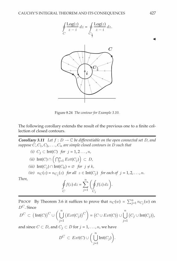
CAUCHY’S INTEGRAL THEOREM AND ITS CONSEQUENCES 427
\
C
Log(z)
z " idz =
\
C 13
Log(z)
z " idz.
"
i
C
C 1
3
Figure 8.24 The contour for Example 3.10.
The following corollary extends the result of the previous one to a finite col-lection of closed contours.
Corollary 3.11 Let f : D 3 C be differentiable on the open connected set D, andsuppose C, C1, C2, . . . , Cn are simple closed contours in D such that
(i) Cj ' Int(C) for j = 1, 2 . . . , n,
(ii) Int(C) &(>n
j=1 Ext(Cj ))
' D,
(iii) Int(Cj) & Int(Ck) = ! for j $= k,
(iv) nC (z) = nCj(z) for all z # Int(Cj) for each of j = 1, 2, . . . , n.
Then, \
C
f (z) dz =n+
j=1
2\
Cj
f (z) dz
3.
PROOF By Theorem 3.6 it suffices to prove that nC (w) =;n
j=1 nCj(w) on
DC . Since
DC'
,Int(C)
-C%
2 n?
j=1
,Ext(Cj )
-C3
=,C % Ext(C)
-%
n?
j=1
,Cj % Int(Cj )
-,
and since C ' D, and Cj ' D for j = 1, . . . , n, we have
DC' Ext(C) %
2 n?
j=1
Int(Cj)
3.

428 COMPLEX INTEGRATION
As in the proof of the previous corollary, if w0 # DC there are two cases toconsider. If w0 # Ext(C), we leave it to the reader to show that Ext(C) '
Ext(Cj ) for j = 1, . . . , n, and hence that nC (w0) = nCj(w0) = 0 so that
nC (w0) =;n
j=1 nCj (w0). If instead w0 #
(#nj=1 Int(Cj )
), then w0 # Int(Cj ) for
some 1 + j + n, and for this j we have nC (w0) = nCj(w0). Since w0 $# Int(Ck)
for k $= j (Why?), we have nCk(w0) = 0 for k $= j. Overall, this obtains in this
second case that nC (w0) =;n
j=1 nCj (w0). #
! 8.48 Complete the proof of the above corollary by showing that when w0 " Ext(C)we have Ext(C) ! Ext(Cj) for j = 1, . . . , n, and hence that nC (w0) = nCj (w0) = 0 sothat nC (w0) =
;n
j=1 nCj (w0). Also, answer the (Why?) question in the above proof.
Example 3.12 For the contour C shown in Figure 8.25, we will show that]
C
dzz2"z
=]
C1
dzz2"z
+]
C2
dzz2"z
where C1 is the parametrized circle of radius !1
centered at the origin, and C2 is the parametrized circle of radius !2 centeredat z = 1. Here, !1 and !2 are to be taken small enough to ensure that C1 and C2
C
C1
C2
Figure 8.25 The situation in Example 3.12.
are contained in Int(C). Verify via the geometric intuition established in Ap-pendix A that nC (0) = nC1
(0) = 1 and that nC (1) = nC2(1) = 1. By confirming
too that the conditions of Corollary 3.11 hold, we have the result. "
4 CAUCHY’S INTEGRAL FORMULA
It is an interesting and useful property of differentiable complex functionsthat they can be appropriately represented by integrals around closed con-tours. Cauchy’s integral formula and the variations of it that follow are notonly of great practical use in computations, they are also fundamental in es-tablishing other results of deep significance in complex function theory.
4.1 The Various Forms of Cauchy’s Integral Formula
We begin with a version of Cauchy’s integral formula on star-shaped sets.

CAUCHY’S INTEGRAL FORMULA 429
Proposition 4.1 (Cauchy’s Integral Formula on Star-Shaped Sets)Let f : D 3 C be differentiable on the open star-shaped set D, and suppose C is aclosed parametrized contour in D. Then for z0 # D \ C,
1
2% i
\
C
f (0)
0 " z0d0 = nC (z0) f (z0).
PROOF Let g : D 3 C be given by g(0) =
Ef (/)"f (z0)
/"z0for 0 # D \ {z0}
f &(z0) for 0 = z0.
Note that g is continuous on D and differentiable on D \ {z0}, and thereforeby Corollary 2.11 on page 408 and Theorem 2.14 on page 411 we have that
0 =
\
C
g(0) d0 =
\
C
f (0)
0 " z0d0 " 2% i nC(z0) f (z0).
A simple rearrangement gives the result. #
! 8.49 Show that the function g described in the proof of the above result is contin-uous on D and differentiable on D \ {z0}.
The following corollary is a useful consequence of the above result.
Corollary 4.2 (Cauchy’s Integral Formula for Circles)Suppose f : D 3 C is differentiable on the open set D, and let Cr be a parametrizedcircle of radius r such that it and its interior are contained in D. Then for z0 #
D \ Cr ,1
2 % i
\
Cr
f (0)
0 " z0d0 =
E0 if z0 # Ext(Cr)
f (z0) if z0 # Int(Cr).
PROOF We first consider the case where z0 is outside Cr. Let D& be an opendisk in D that contains Cr but excludes z0, i.e., Cr ' D&
' D and z0 $# D&.The function F : D&
3 C given by F (0) / f (/)/"z0
is differentiable on D&, and so\
Cr
F (0) d0 =
\
Cr
f (0)
0 " z0d0 = 0. (Why?)
Now consider the case where z0 is inside Cr. Again, let D& be a disk such thatCr ' D&
' D. Apply the previous proposition, and the result is proved. #
! 8.50 How do we know a disk such as D# as described in each of the cases of the
above proof exists? What type of region is D# in each case? To answer these ques-
tions, let Cr be a circle such that it and its interior are contained in the open setD ! C. If r and a are the circle’s radius and center, respectively, show that there

430 COMPLEX INTEGRATION
exists a neighborhood N)(a) such that Cr ! N)(a) ! D. (Hint: Assume otherwise,that is, that for all , > r we have N)(a)$D
C %= !. In particular, show that there existswn " N
r+ 1n
(a) $ DC .)
! 8.51 Suppose the circle in the statement of the above corollary is parametrized sothat it is traversed n " N times in the counterclockwise direction, rather than just
once. Show that this yields the result 12 # i
]
Cr
f (+)+!z0
d* =
E0 if z0 " Ext(Cr)
n f (z0) if z0 " Int(Cr).
What if the circle is traversed in the clockwise direction?
! 8.52 Use Corollary 4.2 to prove Gauss’s mean value theorem. If f : D , C isdifferentiable on the open set D ! C, and Cr(z0) and its interior are contained within
D, then f (z0) = 12#
Z 2#
0 f (z0 + r ei t) dt.
Let Dr / Int(Cr). Then Corollary 4.2 (and also Exercise 8.52) tells us that ifDr ' D and if f is differentiable on D, the values of f inside the disk Dr
are completely determined by the values of f on the boundary of the disk, animportant insight about differentiable complex functions. That is, for z0 #
Dr,
f (z0) =1
2 % i
\
Cr
f (0)
0 " z0d0. (8.12)
Of course, this expression can also be rearranged as\
Cr
f (0)
0 " z0d0 = 2 % i f (z0), (8.13)
highlighting its computational utility in evaluating integrals of this type.
Example 4.3 Note that, for C2 / C2(i), the parametrized circle of radius 2centered at i, the integrals
]
C2
sin zz dz and
]
C2
sin zz"5 i dz can both readily be seen
to equal 0 by virtue of formula (8.13) and Corollary 4.2. "
! 8.53 Use (8.13) to calculate the results of the integrals obtained in Examples 3.7and 3.8 on page 424, and Example 3.10 on page 426.
Next, a generalization of Cauchy’s integral formula to open connected sets.
Theorem 4.4 (Cauchy’s Integral Formula on Open Connected Sets)Let f : D 3 C be differentiable on the open connected set D ' C. Suppose C is aclosed parametrized contour in D and suppose nC (w) = 0 for all w # DC . Then forz0 # D \ C, 1
2% i
\
C
f (0)
0 " z0d0 = nC (z0) f (z0).

CAUCHY’S INTEGRAL FORMULA 431
PROOF Choose r > 0 small enough so that Nr(z0) ' D \C and let GC r2
be the
contour parametrized by Gz : [0, 2%] 3 C, where Gz(t) = z0 + r2 exp
,i nC(z0) t
-
(see Figure 8.26). Then as shown in Exercise 8.30 on page 405, n GC r2
(z0) =
nC (z0). Now, if D0 / D \ {z0} it follows that f (/)/"z0
is differentiable on the
open connected set D0, and C and GC r2
are closed contours in D0. If we can
Nr(z0)
˜Cr2
C
z0
Figure 8.26 The situation described in the proof of Cauchy’s integral formula on open con-nected sets.
show that n GC r2
(w) = nC (w) for all w # DC0 , then by Theorem 3.6 on page 423,
we have \
C
f (0)
0 " z0d0 =
\
GC r2
f (0)
0 " z0d0.
Since f is differentiable on Nr(z0), Cauchy’s integral formula on star-shapedsets yields that
\
GC r2
f (0)
0 " z0d0 = 2% i n GC r
2
(z0) f (z0) = 2% i nC(z0) f (z0).
It remains only to show that n GC r2
(w) = nC (w) for all w # DC0 . To see this,
consider w # DC0 . Then w # DC
% {z0}. If w # DC , then n GC r2
(w) = 0 and
nC (w) = 0, and hence, n GC r2
(w) = nC (w). If w = z0, then n GC r2
(w) = n GC r2
(z0) =
nC (z0) = nC (w), and the theorem is proved. #
Example 4.5 Recall that in Example 3.7 on page 424 we established that]
C1
cos zz dz =
]
C2
cos zz dz for the contours C1 and C2 depicted there. Applying
Corollary 4.2 yields the result that]
C1
cos zz dz =
]
C2
cos zz dz = 1
2$ i . Likewise, in
Example 3.8 we established that]
C
dz(z"z1) (z"z2) =
]
C1
dz(z"z1) (z"z2) +
]
C2
dz(z"z1) (z"z2) .

432 COMPLEX INTEGRATION
Once again, by applying Corollary 4.2 we obtain\
C
dz
(z " z1) (z " z2)=
\
C1
dz
(z " z1) (z " z2)+
\
C2
dz
(z " z1) (z " z2)
= ("1)1
2% i
1
(z1 " z2)+ ("1)
1
2% i
1
(z2 " z1). "
! 8.54 Reconsider Example 3.12 on page 428 , and show via Cauchy’s integral for-mula that the integral there is equal to 0.
In practice, a frequent case to consider is that where z belongs to a connectedsubset of D \ C, and nC (z) = 1. Then,
f (z) =1
2% i
\
C
f (0)
0 " zd0
for all z in this connected set. In fact, we have the following result.
Corollary 4.6 (Cauchy’s Integral Formula for Simple Closed Contours)Let f : D 3 C be differentiable on the open set D ' C, and suppose C is a simpleclosed parametrized contour such that C and Int(C) are contained in D. If nC (z) = 1for all z # Int(C), then for any z0 # Int(C),
1
2% i
\
C
f (0)
0 " z0d0 = f (z0).
! 8.55 Prove the above corollary.
Note that determining that nC (z) = 1 for a particular simple closed contourC and a point z # Int(C) is usually accomplished through the geometric in-tuition developed in the Appendices section of this chapter (see the sectionpreceding the Supplementary Exercises). An actual computation of nC (z) forsuch a simple closed contour is not generally necessary. For a single traver-sal of a specific contour such as that described here, one can trace the con-tour starting from the initial/terminal point and note that the continuouslychanging argument has a net increase of 2% when one arrives back at theinitial/terminal point. This is enough to imply that the associated windingnumber for the contour is 1. The reader is encouraged to read the Appendicessection now.
Example 4.7 We will use Corollary 4.6 to evaluate]
C
ez
z dz where C is the
parametrized square [2 + 2 i,"2 + 2 i,"2" 2 i, 2" 2 i, 2 + 2 i]. Simply note thatez is differentiable on C, and therefore by the above corollary the integral isequal to 2% i. "

CAUCHY’S INTEGRAL FORMULA 433
Example 4.8 We will evaluate]
C 12
dzz3"z
where C 12/ C 1
2(1) is the parametrized
circle centered at z = 1 of radius 12 . If we consider f : D 3 C where
f (z) = 1z (z+1) and D = {z # C : |z " 1| < 3
4}, then f is differentiable onD, and C 1
2and its interior are contained in D. By Cauchy’s integral formula
for circles, we have \
C 12
dz
z3" z
= 2% i f (1) = 2% i,
12
-= % i.
"
4.2 The Maximum Modulus Theorem
We present one more important property of differentiable complex functions.Our proof of it relies on the application of Cauchy’s integral formula. Calledthe maximum modulus theorem, it establishes that if a differentiable complexfunction on D ' C is such that |f | attains a local maximum at a # D, then|f | must equal that maximum value throughout some neighborhood Nr(a) ' D.Even more than this is true, namely, there exists some constant c # C suchthat |c| = |f (a)| and for which f (z) = c throughout Nr(a). This result is nottrue generally for differentiable functions in any of the real cases we haveconsidered.4
Theorem 4.9 (Maximum Modulus Theorem—First Version)Suppose f : D 3 C is differentiable on the open connected set D ' C and that forsome a # D there exists NR(a) ' D such that |f (z)| + |f (a)| for all z # NR(a).Then f (z) = f (a) for all z # NR(a).
PROOF Choose 0 < r < R, and define Cr / Cr(a) to be the parametrizedcircle of radius r centered at a. Then
f (a) =1
2% i
\
Cr
f (z)
z " adz
=1
2% i
Y 2$
0
f (a + r eit)
r eiti r eit dt
=1
2%
Y 2$
0f (a + r eit) dt.
Therefore,
|f (a)| +1
2%
Y 2$
0|f (a + r eit)| dt +
1
2%
Y 2$
0|f (a)| dt = |f (a)|,
4In fact, it is true for the special case of harmonic functions u : D2 ( R, but not moregenerally among real differentiable functions. Of course, a differentiable complex function f =u + iv has harmonic functions u and v as its real and imaginary parts!

434 COMPLEX INTEGRATION
which implies that
1
2%
Y 2$
0|f (a + r eit)| dt = |f (a)| =
1
2%
Y 2$
0|f (a)| dt.
From this we have, Y 2$
0
(|f (a + r eit)|" |f (a)|
)dt = 0.
But since |f (a + r eit)| + |f (a)|, it follows that |f (a + r eit)| " |f (a)| + 0, andhence that
|f (a + r eit)|" |f (a)| = 0. (Why?)
Overall then, we have that
|f (a + r eit)| = |f (a)| for all 0 < r < R, and for all t # [0, 2%],
which means that|f (z)| = |f (a)| for all z # NR(a).
Finally, we see that f maps a small neighborhood of z into a circle. Takingderivatives in different directions, it follows from the Cauchy-Riemann equa-tions that f (z) = c on NR(a) for some constant c # C. The value of c mustclearly be f (a). #
! 8.56 Justify the conclusion of the proof of the above theorem.
Actually, it can be shown that if f satisfies the conditions of the above theo-rem, it must equal c on all of D. This is even more surprising, but requires abit more work to establish.5 An extension of the above theorem that we willprovide is the following.
Theorem 4.10 (Maximum Modulus Theorem—Second Version)Let D ' C be bounded, open, and connected. Suppose f : D 3 C is differentiableon D and continuous on D. Then the maximum value of |f | on D is attained on theboundary *D. If the maximum of |f | is also attained on the interior of D, then fmust be constant on D.
PROOF We follow a proof idea as described in [MH98]. Let M = maxD
|f (z)| =
|f (a)| for some a # D. If a # *D we are done. So assume a # D. Define
D1 / {z # D : f (z) = f (a)} and D2 / D \ D1.
We will establish the following:1. D ' D1 % D2.
2. D1 & D2 = !.
3. D1 is open.
5The proof involves the idea of analytic continuation of a differentiable complex function. See[MH98].

CAUCHY’S INTEGRAL FORMULA 435
4. D2 is open.
To establish 1, let z0 be an arbitrary point in D. If z0 # D2, we are done. Ifz0 $# D2, then z0 # D1. (Why?) Choosing a sequence {zn} ' D1 such thatlim zn = z0, continuity of f then implies that lim f (zn) = f (z0). But f (zn) =f (a) for all n # N, and so it follows that f (z0) = f (a) and therefore z0 # D1.To prove 2, suppose there exists z0 # D1 & D2. Then z0 # D1 (Why?) andz0 # D2 = D \ D1, a contradiction. Therefore, D1 & D2 = !. To establish 3, letz0 be an element of D1. Then |f (z0)| = |f (a)| = M . Since D is open there existsa neighborhood NR(z0) ' D, and
|f (z)| + M = |f (a)| = |f (z0)| on NR(z0).
From the first version of the maximum modulus theorem it follows thatf (z) = f (z0) = f (a) on NR(z0), that is, NR(z0) ' D1. Therefore D1 is open.Finally to prove 4, note that D2 = D \ D1 = D & (D1)C , the intersection ofopen sets. Therefore D2 is open. With 1–4 established, since D is connected,it must follow that either D1 = ! or D2 = !. But a # D1, so it must be the casethat D2 = !. This and 1 then implies that D ' D1, and therefore f (z) = f (a)for all z # D. By continuity, this implies f (z) = f (a) for all z # D. This saysthat |f (z)| = M on D as well as on D, and the proof is complete. #
! 8.57 Let D ! C be bounded, open and connected. Suppose the complex functionf : D , C is nonconstant and differentiable on D and continuous on D. What doesthe above theorem allow you to conclude about the location of the maximum value off on D? How does this differ from the case where f is a real-valued function of twovariables?
4.3 Cauchy’s Integral Formula for Higher-Order Derivatives
The following proposition is a valuable tool.
Proposition 4.11 Let f : D 3 C be continuous on the open set D ' C, and let Cbe a parametrized contour in D. For each n # N define Fn : C \ C 3 C accordingto
Fn(z) /
Y
C
f (0)
(0 " z)nd0.
Then for each n # N the function Fn is differentiable on C \ C, and
F &n(z) = n
Y
C
f (0)
(0 " z)n+1d0 = n Fn+1(z) for all z # C \ C.
Note that this result says that under the conditions of the proposition, wemay differentiate under the integral sign, i.e.,
F &n(z) = n
Y
C
f (0)
(0 " z)n+1d0 =
Y
C
d
dz
2f (0)
(0 " z)n
3d0.

436 COMPLEX INTEGRATION
PROOF We will establish the result for n = 1 and leave the general case tothe reader. Let z0 # D \ C and choose + > 0 such that N%(z0) ' D \ C. Forany ! > 0, we will find . > 0 such that
z # D & N+(z0) )
&&&&F1(z) " F1(z0) "
2Y
C
f (0)
(0 " z0)2d0
3(z " z0)
&&&& + ! |z " z0|.
To see this, note that for z # N %2
(z0) we have&&&&F1(z) " F1(z0)"
2Y
C
f (0)
(0 " z0)2d0
3(z " z0)
&&&&
=
&&&&
Y
C
f (0)
0 " zd0 "
Y
C
f (0)
0 " z0d0 "
2Y
C
f (0)
(0 " z0)2d0
3(z " z0)
&&&&
=
&&&&
2Y
C
f (0)
(0 " z)(0 " z0)d0 "
Y
C
f (0)
(0 " z0)2d0
3(z " z0)
&&&&
=
&&&&(z " z0)
Y
C
(0 " z0)(z " z0)f (0)
(0 " z0)3(0 " z)d0
&&&&
= (z " z0)2
&&&&
Y
C
f (0)
(0 " z0)2(0 " z)d0
&&&&.
Now for 0 # C and z # N %2
(z0), it follows that
1. |f (0)| + " / max/#C
|f (0)|,
2. |0 " z0| ! +,
3. |0 " z| ! %2 ,
and therefore for |z " z0| < ( %3
2 " LC/ .,
&&&&F1(z) " F1(z0) "
2Y
C
f (0)
(0 " z0)2d0
3(z " z0)
&&&& + |z " z0|2 2 " LC
+3
+ ! |z " z0|.
Therefore, F &1(z) =
Z
C
f (/)(/"z0)2 d0 and the proof of the n = 1 case is complete. #
! 8.58 Prove the general case.
Using the above proposition, one can now prove the following result, a kindof converse to Corollary 4.6.
Corollary 4.12 Let f : D 3 C be continuous on the open connected set D ' C.Suppose that for every z0 # D and every simple closed parametrized contour C
CAUCHY’S INTEGRAL FORMULA 437
satisfying the following conditions,
(i) z0 # Int(C),
(ii) C and Int(C) are contained in D,
we havef (z0) =
1
2% i
\
C
f (0)
0 " z0d0.
Then f is differentiable on D.
! 8.59 Prove the above corollary to Proposition 4.11
The following corollary is a surprising and potent extension of the idea rep-resented by equation (8.12) on page 430.
Corollary 4.13 Suppose f : D 3 C is differentiable on the open connected set D,and let C be a closed parametrized contour contained in D. Then for any z0 # D\C,
nC (z0) f (n)(z0) =n!
2 % i
\
C
f (0)
(0 " z0)n+1d0 for n = 0, 1, 2, . . . . (8.14)
Also, for " and r defined by " / max/#C
|f (0)| and r / min/#C
|0 " z0|,
&&nC (z0) f (n)(z0)&&+
n! " LC
2% rn+1. (8.15)
Expressions (8.14) and (8.15) in Corollary 4.13 are known as Cauchy’s integralformulas for the derivatives and Cauchy’s inequalities, respectively.
! 8.60 Prove the above corollary using Proposition 4.11.
! 8.61 In the special case where C = Cr(z0), a circle of radius r centered at z0, show
that (8.15) in the above corollary reduces to&&f (n)(z0)
&& # n! "rn .
The above corollary tells us some very significant things about a complexfunction f : D 3 C that is differentiable on the open connected set D.
1. It tells us that such a function has derivatives of all orders inside D, and
provides a formula for computing any derivative of f inside D.
2. It tells us that for any z0 # Int(C) ' D, the values of f and its derivatives
of all orders at z0 are determined by the values of f on the boundary of thedisk Dr ' D centered at z0.
The first fact is significant enough to state as a separate corollary.

438 COMPLEX INTEGRATION
Corollary 4.14 If f : D 3 C is differentiable at z0 in the open set D, then f isinfinitely differentiable at z0 # D.
It is important to note that while the above corollary is true for differentiablecomplex functions f : D 3 C, it does not hold for any of the real functionclasses we have studied thus far. For example, it is not true that all differen-tiable functions f : R 3 R are necessarily infinitely differentiable, nor is ittrue that all differentiable functions f : Rk
3 Rm are necessarily infinitelydifferentiable, and so on. This is one of the significant ways in which complexfunctions distinguish themselves from real functions.
5 FURTHER PROPERTIES OF COMPLEX DIFFERENTIABLE
FUNCTIONS
5.1 Harmonic Functions
There is a special subclass of real functions u : D23 R called harmonic func-
tions to which Corollary 4.14 does apply. And it is no coincidence that thissubclass of real-valued functions is directly related to the class of differen-tiable complex functions, as the next corollary shows.
Corollary 5.1 If f : D 3 C given by f = u + i v is differentiable on the open setD ' C, then u, v : D2
3 R, where D2 is the set D as represented in the xy-plane,are each twice differentiable and satisfy
#u /
*2u
*x2+
*2u
*y2= 0 and #v /
*2v
*x2+
*2v
*y2= 0
on D2. That is, u and v are harmonic functions.
PROOF Since f = u + i v is differentiable on D, the Cauchy-Riemann equa-tions yield -u
-x = -v-y and -u
-y = "-v-x . Since f & = -u
-x + i -v-x = -v
-y " i -u-y is also
differentiable on D, the Cauchy-Riemann equations applied once again yield
*2u
*x2=
*2v
*y*x,
*2u
*y2= "
*2v
*x*y,
and*2v
*x2= "
*2u
*y*x,
*2v
*y2=
*2u
*x*y.
These equations together, along with the mixed derivative theorem, imply#u = #v = 0. #
A special relationship exists between the functions u and v in the case wheref : D 3 C given by f = u + iv is a differentiable complex function. From
FURTHER PROPERTIES OF COMPLEX DIFFERENTIABLE FUNCTIONS 439
Corollary 5.1 we know that u and v must both be harmonic on D2, the ver-sion of D in R2. But this is not all. The functions u and v must also satisfythe Cauchy-Riemann equations, a condition that forces them to be what arecalled harmonic conjugates of each other. This is illustrated in the followingexample.
Example 5.2 Suppose u : R23 R is given by u(x, y) = x2
" y2. Can we finda function v : R2
3 R such that the complex function f : C 3 C wheref = u + iv is differentiable? If so, is the associated v unique? Before lookingfor such a v, note that for the given u we have that #u / 0 on R2. Thereforeaccording to Corollary 5.1, the function u might be the associated real partof a differentiable complex function f = u + iv. Of course, any v we seekas the imaginary part of f must also satisfy #v / 0 on R2, but if f is tobe differentiable u and v must also satisfy the Cauchy-Riemann equations,namely, ux = vy and uy = "vx on R2. Therefore, since ux = 2 x, we must havevy = 2 x. Integrating this last equation with respect to y obtains v = 2 xy+k(x).Note that the constant of integration associated with the y partial integrationmight actually be a function of x. From this candidate for v we see that vx =2 y + k&(x). And since "uy = 2 y the Cauchy-Riemann equations imply that2 y + k&(x) = 2 y, or k&(x) = 0. That is, k(x) / c # R, a constant. Overall then,any function v : R2
3 R of the form v = 2 xy+c will work. It is easy to see thatour discovered form for v satisfies the condition #v / 0 as well. Any such vis called a harmonic conjugate of u = x2
" y2 on R2. The reader should checkthat u is a harmonic conjugate of v on R2. "
! 8.62 Given v : R2 , R where v(x, y) = 2xy, show that there exists a harmonic
function u : R2 , R such that f : C , C given by f = u + iv is a differentiable
complex function on C, and that u has the form u(x, y) = x2 & y
2 + c for arbitraryconstant c " R.
! 8.63 If u : D2 , R is harmonic on D
2, then u is C%(D2). In fact, u = Re(f ) for
some differentiable complex function f : D , C, where D is D2 as represented in C.
Note that this result only holds locally, even if D is connected. To see this, consideru : D
2 , R given by u(x, y) = ln(x2 + y2) where D
2 = R2 \ {0}. Determine the
harmonic conjugates of u. How do they differ from each other? What is the domainof the resulting differentiable complex function f?
5.2 A Limit Result
The following result will be of use to us in the next chapter. Its proof, perhapssurprisingly, requires the use of Cauchy’s integral formula.
Theorem 5.3 Let fn : D 3 C be differentiable on D for n ! 1 and suppose thereexists a function f : D 3 C such that lim
n('fn(z) = f (z) uniformly on D. Then f
is differentiable on D and f &(z) = limn('
f &n(z) on D.

440 COMPLEX INTEGRATION
PROOF Fix a # D, and choose the parametrized circle Cr / Cr(a) such thatCr and its interior belong to D. Then Cauchy’s integral formula obtains
fn(z) =1
2%i
\
Cr
fn(0)
0 " zd0 for |z " a| < r.
We ask the reader to show that for fixed z,
limn('
\
Cr
fn(0)
0 " zd0 =
\
Cr
f (0)
0 " zd0.
This implies
f (z) =1
2%i
\
Cr
f (0)
0 " zd0 for |z " a| < r,
and so by Proposition 4.11 we have
f &(z) =1
2%i
\
Cr
f (0)
(0 " z)2d0 for |z " a| < r.
Finally, we know that
f &n(z) =
1
2%i
\
Cr
fn(0)
(0 " z)2d0 for |z " a| < r,
which yields
limn('
f &n(z) =
1
2%i
\
Cr
f (0)
(0 " z)2d0 = f &(z) for |z " a| < r.
#
! 8.64 For fixed z, show that limn&%
]
Cr
fn(+)+!z
d* =]
Cr
f (+)+!z
d*, and thereby complete the
proof of the above theorem.
5.3 Morera’s Theorem
The following result is a kind of converse to Cauchy’s integral theorem. Itsproof requires Cauchy’s integral formula, however, and so we present it hererather than in the previous section.
Theorem 5.4 (Morera’s Theorem)Let f : D 3 C be continuous on the open set D ' C such that
]
C
f (z) dz = 0 for
every closed contour C ' D. Then f is differentiable on D.
PROOF Fix z0 # D. We will show that f is differentiable at z0. To this end,

FURTHER PROPERTIES OF COMPLEX DIFFERENTIABLE FUNCTIONS 441
consider Nr(z0) ' D, and define F : Nr(z0) 3 C by
F (z) /
Y
[z0,z]
f (0) d0.
By the path-independence of integrals of continuous functions in star-shapedregions, for any triangle = ' Nr(z0) we have that
]
/f (0) d0 = 0. It then fol-
lows by an argument similar to that in the proof of Theorem 2.14 on page 411that F is differentiable on Nr(z0), and F &(z) = f (z). By Corollary 4.14 onpage 438, F is infinitely differentiable on Nr(z0), which implies that f is alsoinfinitely differentiable on Nr(z0), and hence at z0. #
! 8.65 Let f : D , C be continuous on the open set D ! C, and suppose f isdifferentiable on D \ {p} for some p " D. Show that f is differentiable on all of D.What if f is presumed initially to only be differentiable on D \ {z1, z2, . . . , zn} forz1, z2, . . . , zn " D?
5.4 Liouville’s Theorem
The next result pertains to complex functions that are differentiable in theentire complex plane. Such functions are called, appropriately enough, entirefunctions. The result follows the formal definition.
Definition 5.5 A function f : C 3 C that is differentiable on all of C is calledan entire function.
Constant functions and polynomials are entire. The following theorem mayseem surprising at first.
Theorem 5.6 (Liouville’s Theorem)If f : C 3 C is entire and bounded, then f (z) / c for some constant c # C.
PROOF The proof of this result is almost as surprising as the result itself.In fact, it is surprisingly simple. If f is to be shown to be constant, then weshould be able to show that its derivative is identically zero. Suppose |f (z)| +M for all z # C. Then fix an arbitrary z0 # C and let C be a circle of radius Rcentered at z0. By Corollary 4.13 on page 437, we have
f &(z0) =1
2 % i
\
C
f (z)
(z " z0)2 dz,
and
|f &(z0)| +1
2 %
M
R2(2 % R) =
M
R. (8.16)
Note that (8.16) is true for any R > 0. If ! > 0 is given, choose R large enoughsuch that

442 COMPLEX INTEGRATION
|f &(z0)| +M
R< !,
which implies that f &(z0) = 0. Since z0 # C was arbitrary, f &(z) = 0 for allz # C, and so f must be constant on C. #
5.5 The Fundamental Theorem of Algebra
Liouville’s theorem is useful in proving the following famous result.
Theorem 5.7 (The Fundamental Theorem of Algebra)If p : C 3 C is a nonconstant polynomial given by
p(z) = a0 + a1 z + · · · + aN zN , where aN $= 0 and N ! 1,
then there exists z0 # C such that p(z0) = 0, i.e., the polynomial p(z) has at least oneroot.
PROOF Assume p(z) has no roots. Then the function f : C 3 C given byf (z) = 1
p(z) is entire. We will show that f is bounded, and hence, by Liouville’s
theorem, constant (a contradiction). To see that f must be bounded, note
|f (z)| =1
|p(z)|+
1&&&|aN zN|" |a0 + a1 z + · · · + aN"1 zN"1
|
&&&. (8.17)
But,
|a0 + a1 z + · · ·+aN"1 zN"1|
+
,max
k|ak|
- ,1 + |z| + · · · + |z|N"1-
=,
maxk
|ak|- 1 " |z|N
1 " |z|
+ |aN |
,|z|" 1
- |z|N " 1
|z|" 1for |z| > R sufficiently large,
= |aN | |z|N " |aN |
= |aN zN|" |aN |. (8.18)
The “sufficiently large“ R referred to above can be any value greater thanmaxk |ak|
|aN | + 1. Subbing (8.18) into (8.17) obtains
|f (z)| =1
|p(z)|+
1
|aN |
/ c for |z| > R.
From this, we have that f is bounded by c outside the disk of radius R. Butsince the closed disk of radius R is a compact set, there exists M such that|f | < M on the closed disk. Overall then, we have |f | + max (M , c), andhence, f is bounded. By Liouville’s theorem f must be constant, a contradic-tion. #

APPENDICES: WINDING NUMBERS REVISITED 443
The following corollary to the fundamental theorem of algebra is a frequentlyexploited fact, namely, that any polynomial of degree N # N with real orcomplex coefficients has exactly N roots, including multiplicities. We prefaceits more formal statement with some terminology. Note that if z1 is a root ofthe polynomial p(z), we may write p(z) as follows,6
p(z) = (z " z1) q1(z),
where q1(z) is a polynomial of degree one less than that of p(z). If z1 is a rootof q1(z), we may repeat the procedure and obtain
p(z) = (z " z1)2 q2(z),
where q2(z) is a polynomial of degree one less than that of q1(z). We maycontinue in this way until z1 is no longer a root of qm1 for some m1 # N,yielding
p(z) = (z " z1)m1 qm1 (z).
We then say that p(z) has root z1 with multiplicity m1. Doing this for each rootof p(z), and accounting for each root’s multiplicity, we obtain the followingresult.
Corollary 5.8 Suppose p : C 3 C is a nonconstant polynomial given by
p(z) = a0 + a1 z + · · · + aN zN , where aN $= 0 and N # N.
If z1, z2, . . . , zr are the distinct roots of p, with associated multiplicities m1, m2, . . . ,mr, then
;rj=1 mj = N , and p(z) can be written as
p(z) = c (z " z1)m1 (z " z2)m2· · · (z " zr)mr
for some constant c # C.
! 8.66 Prove the above corollary.
6 APPENDICES: WINDING NUMBERS REVISITED
6.1 A Geometric Interpretation
In this appendix, we will establish a useful geometric interpretation of thewinding number nC (z0) of a curve C ' C about a fixed point z0 # C. In par-ticular, nC (z0) can be interpreted as the number of times the curve C “windsaround“ the point z0. To establish this, we will need to prove several technicalresults.
Continuous Logarithms and Arguments
For the following four lemmas, we follow [AN07]. The results are actuallyspecial cases of more general theorems about “covering spaces” in topology,for which we refer the reader to [Hat02].
6See any introductory text in abstract algebra.

444 COMPLEX INTEGRATION
Lemma 6.1 Let z : [a, b] 3 C be continuous on [a, b] such that z(t) $= 0 for allt # [a, b]. There exists a continuous function g : [a, b] 3 C such that z(t) = eg(t)
for all t # [a, b].
The function g is sometimes called a continuous logarithm of z. This resultwould probably seem obvious if the complex z were replaced by real x > 0.
m
Nm(z(tj!1))
Figure 8.27 The proof of Lemma 6.1.
PROOF As depicted in Figure 8.27, let m / mint'[a,b]
|z(t)| > 0. Since z is uni-
formly continuous on [a, b], there exists . > 0 such that
|t " t&| < . ) |z(t) " z(t&)| < m.
Let P = {a = t0, t1, . . . , tn = b} be a partition of [a, b] with 2P2 < .. It followsthat for each 1 + j + n,
z(t) # Nm,z(tj"1)
-for t # [tj"1, tj]. (Why?)
Since 0 $# Nm,z(tj"1)
-for 1 + j + n, there exists a continuous function
hj : Nm,z(tj"1)
-3 C such that
0 = ehj(/) for all 0 # Nm,z(tj"1)
-.
Note here that hj is a branch of the complex logarithm (and is therefore dif-ferentiable on Nm
,z(tj"1)
-), and that it takes complex arguments; the g we
seek will take real arguments. We’ll now restrict this hj to points on the con-tour within Nm
,z(tj"1)
-. Since z(t) # Nm
,z(tj"1)
-for all t # [tj"1, tj], we
havez(t) = ehj
,z(t)
-for t # [tj"1, tj].
Now define gj : [tj"1, tj] 3 C for 1 + j + n according to gj(t) / hj
,z(t)
-for
t # [tj"1, tj]. Then,

APPENDICES: WINDING NUMBERS REVISITED 445
z(t) = eg1(t) for t # [a, t1],
z(t) = eg2(t) for t # [t1, t2],
......
z(t) = egn(t) for t # [tn"1, b].
Note that g2(t1) = g1(t1) + 2% i N for some N # Z (Why?), so that we mayreplace g2 by g2 " 2% i N and define g : [a, t2] 3 C by
g(t) =
Eg1(t) for t # [a, t1]
g2(t) " 2% i N for t # [t1, t2].
Then g is continuous on [a, t2] (Why?), and we have that z(t) = eg(t) for t #
[a, t2]. Continuing in this way, we can define g on [a, t3], and eventually onall of [a, b] such that g is continuous on [a, b], and z(t) = eg(t) on [a, b]. #
If g is a continuous logarithm of z, it is reasonable to consider g(z) as log z =ln |z| + i arg z, and to therefore expect that arg z can be chosen to be continu-ous. We prove this next.
Lemma 6.2 Let z : [a, b] 3 C be a continuous function on [a, b] such that z(t) $= 0for all t # [a, b]. Then there exists $ : [a, b] 3 R continuous on [a, b] such thatz(t) = |z(t)| ei"(t) for all t # [a, b].
PROOF By the previous lemma there exists g : [a, b] 3 C continuous on[a, b] such that z(t) = eg(t) for all t # [a, b]. From this we have
z(t) = eg(t) = eRe(g(t))+i Im(g(t)) = eRe(g(t)) ei Im(g(t)),
and therefore, |z(t)| = eRe(g(t)). Defining $ : [a, b] 3 R by $(t) / Im(g(t)), wehave
z(t) = |z(t)| ei "(t). #
Two more technical results are required. The first one says that if you havetwo continuous logarithms of z, then they can differ by only a multiple of2% i. Likewise, their arguments can differ only by a multiple of 2%.
Lemma 6.3 Let z : [a, b] 3 C be a continuous function on [a, b] such that z(t) $= 0for all t # [a, b]. Suppose g1, g2 : [a, b] 3 C and $1, $2 : [a, b] 3 R are continuouson [a, b] such that
z(t) = eg1(t) = eg2(t) = |z(t)| ei "1(t) = |z(t)| ei "2(t) for all t # [a, b].
Then, for some m, n # Z,
g2(t) = g1(t) + 2% i n, and $2(t) = $1(t) + 2% m.

446 COMPLEX INTEGRATION
PROOF Note that since eg1(t) = eg2(t) for all t # [a, b], we have eg1(t)"g2(t) = 1 =e2$in for some n # Z, and so g1(t) " g2(t) = 2%in or g1(t)"g2(t)
2$i = n. Therefore
the function h : [a, b] 3 C given by h(t) /g2(t)"g1(t)
2$ i is integer-valued, i.e.,h(t) = n(t). The function h is also continuous on [a, b]. Since [a, b] is connected,g2(t)"g1(t)
2$ i / n on [a, b] for some fixed n # Z. A similar argument obtains the
conclusion that "2(t)""1(t)2$ / m on [a, b] for some fixed m # Z, and the lemma
is proved. #
Lemma 6.4 Let z : [a, b] 3 C be a continuous function on [a, b] such that z(t) $= 0for all t # [a, b]. Let g : [a, b] 3 C and $ : [a, b] 3 R be continuous on [a, b] suchthat z(t) = eg(t) = |z(t)| ei "(t). Then, for t1, t2 # [a, b],
g(t2) " g(t1) = ln |z(t2)|" ln |z(t1)| + i,$(t2) " $(t1)
-.
PROOF Let h : [a, b] 3 C be given by h(t) / ln |z(t)| + i $(t). Then,
z(t) = eh(t) = |z(t)| ei "(t),
and by Lemma 6.3 there exists n # N such that
g(t) = h(t) + 2% i n = ln |z(t)| + i $(t) + 2% i n.
The result follows. #
Winding Numbers and the Logarithm
And now the key result. We continue to follow [AN07].
Theorem 6.5 Let C be a closed contour in C parametrized by z : [a, b] 3 C, andsuppose z0 $# C. Choose $ : [a, b] 3 R to be a continuous argument of z(t) " z0.Then,
nC (z0) =1
2%
,$(b) " $(a)
-.
PROOF Let r / dist(z0, C) = mint'[a,b]
|z(t) " z0| > 0. Since z(t) is uniformly
continuous on [a, b], there exists . > 0 such that
|t " t&| < . ) |z(t) " z(t&)| < r.
Choose a partition P = {a = t0, t1, . . . , tn = b} of [a, b] such that 2P2 < ..Then, for t # [tj"1, tj], we have that z(t) # Nr
,z(tj"1)
-while z0 $# Nr
,z(tj"1)
-.
For all 0 # Nr,z(tj"1)
-we have 0 " z0 $= 0. Therefore, there exists hj :
Nr
,z(tj"1)
-3 C differentiable on Nr
,z(tj"1)
-, where hj is the restriction
of a branch of the logarithm function onto Nr
,z(tj"1)
-. Then
0 " z0 = ehj (/) for all 0 # Nr,z(tj"1)
-.
It then follows that

APPENDICES: WINDING NUMBERS REVISITED 447
z(t) " z0 = ehj
,z(t)
-for t # [tj"1, tj]. (8.19)
If we define gj : [tj"1, tj] 3 C for 1 + j + n according to gj(t) / hj
,z(t)
-for
t # [tj"1, tj], equality (8.19) becomes
z(t) " z0 = egj (t) for t # [tj"1, tj ].
Therefore, g&j(t) = z!(t)z(t)"z0
. From this and Lemma 6.4, we have
Y
Cj
dz
z " z0=
Y tj
tj"1
z&(t)
z(t) " z0dt
= gj(tj) " gj(tj"1)
= ln |z(tj) " z0|" ln |z(tj"1) " z0| + i,$(tj) " $(tj"1)
-,
and\
C
dz
z " z0=
n+
j=1
2Y
Cj
dz
z " z0
3= i
,$(b) " $(a)
-.
The result follows. #
6.2 Winding Numbers of Simple Closed Contours
In this subsection, we establish that when traversing a simple closed contourin the plane, the winding number around any interior point is either +1 or"1. We begin with a lemma corresponding to a special case. In its statement,we denote the upper half-plane of C by HU / {z # C : Im(z) > 0}, and thelower half-plane by HL / {z # C : Im(z) < 0}. We follow [Ful97] in theproofs.
Lemma 6.6 Suppose C ' C is a parametrized closed contour that does not containthe point P . Suppose also that there exist points zU # C & HU and zL # C & HL.Let A be the subcontour of C that begins at zL and terminates at zU , and let B bethe subcontour of C that begins at zU and terminates at zL. Suppose A and B havethe following properties:
(i) A & ("-, P ) = !,
(ii) B & (P ,-) = !.
Then nC (P ) = +1.
PROOF Without loss in generality, assume P # R. Parametrize a circle C&
around P such that C does not intersect C& or its interior. Let z1 and z2 bepoints on C& as shown in Figure 8.28, with GA the clockwise arc from z1 to z2,

448 COMPLEX INTEGRATION
P
z1
z2
C"AB
zU
zL
Figure 8.28 The situation in Lemma 6.6.
and GB the clockwise arc from z2 to z1. Define the contours 2A and 2B by
2A /
,A, [zU , z1], GA, [z2, zL]
-,
2B /
,B, [zL, z2], GB, [z1, zU ]
-.
It follows thatn2A(P ) + n2B (P ) = nC (P ) + nC! (P ).
Since 2A & ("-, P ) = !, we conclude that n2A(P ) = 0. Similarly, since 2B &
(P ,-) = !, it follows that n2B (P ) = 0. Therefore,
nC (P ) = "nC!(P ) = 1. #
And now we present the key result of this subsection.
Theorem 6.7 Let C be a parametrized simple closed contour. Then nC (P ) = "1for every P # Int(C), or nC (P ) = +1 for every P # Int(C).
PROOF Without loss of generality, we may assume that C is positioned sothat the following all hold for some parametrization z : [a, b] 3 C (see Figure8.29).
1. C lies in the right half-plane, i.e., Re,z(t)
-> 0 for all t # [a, b],
2. S / min C & (0,-), and T / max C & (0,-),
3. M = z(a) is in the lower half-plane, and N = z(u) is in the upper half-planefor some u with a < u < b,
4. [0, M ] & C = {M} and [0, N ] & C = {N},
5. A / z,[a, u]
-, and B / z
,[u, b]
-,
6. 2A /
,[0, M ], A, [N , 0]
-and 2B /
,[0, M ],"B, [N , 0]
-.

APPENDICES: WINDING NUMBERS REVISITED 449
N = z(u)
0
M = z(a)
Q S S" T " T
P
Figure 8.29 The conditions imposed on the contour C in the proof of Theorem 6.7.
Since C = (A, B), and A & B = {M , N}, it follows that T # A or T # B.We will consider the case where T # A and leave the other case, which ishandled similarly, to the reader. Assuming T # A, we note that [T ,-) doesnot intersect 2B , and therefore,
n2B (T ) = 0.
If 0 < Q < S, then by Lemma 6.6 we have
n2A (Q) = n2B (Q) = 1.
We now show that S # B. To do so, suppose instead that S # A. Note thatthe subcontour of A that connects S to T never intersects 2B , and therefore
n2B (S) = n2B (T ) = 0.
Since [Q, S] also never intersects 2B , we have
n2B (S) = n2B (Q) = 1,
a contradiction. Therefore, S # B. We now define
T &/ min A & (0,-) and S&
/ max B & (0, T &).
Note that the interval (S&, T &) contains no points of A%B. If we take any pointP # (S&, T &), then
nC (P ) = n2A (P ) " n2B (P ). (8.20)But note also that
n2A(P ) = n2A(S&) = n2A(S) = n2A(Q) = 1, (Why?)and
n2B (P ) = n2B (T &) = n2B (T ) = 0. (Why?)
From this, and (8.20), we have
nC (P ) = n2A (P ) " n2B (P ) = 1.
Note that P must be in the interior of C, since nC (W ) = 0 for all W #
Ext(C). #

450 COMPLEX INTEGRATION
! 8.67 Complete the above proof by considering the case where T " B. In this case,show that nC (P ) = &1 for P " Int(C).
7 SUPPLEMENTARY EXERCISES
1. EvaluateZ 2
1
(1t& i t
)2dt.
2. Suppose w : [&a, a] , C is an even function, i.e., w(&t) = w(t) for all t " [&a, a].Show that
Za
!aw(t) dt = 2
Za
0 w(t) dt. What if w(t) is odd, i.e., w(&t) = &w(t) for allt " [&a, a]?
3. EvaluateZ 1
0 ez0t dt, where z0 %= 0 is some complex constant.
4. Let z0, z1, z2 " C form a triangle, T = [z0, z1, z2, z0], in C. For the parametrized T ,write down the explicit parametrization z as described in Definition 1.8.
5. Let z0, z1, z2, z3 " C form a rectangle, R = [z0, z1, z2, z3, z0], in C. For the parametrizedR, write down the explicit parametrization z as described in Definition 1.8.
6. Let D2 = {(x, y) " R
2 : x > 0, y = sin(
1x
)}0{(0, y) " R
2 : &1 # y # 1}. Show that
D2 is connected but is not contour connected. In fact, D
2 is not even path connected.Does this contradict Exercise 8.9 on page 393?
7. Evaluate]
C
z dz if C is the parametrized circle Cr(0).
8. Let f : C , C be given by f (z) = Im(z) + i Re(z). EvaluateZ
C1
f (z) dz andZ
C2
f (z) dz
where C1 and C2 are the parametrized polygonal contours given by C1 = [0, i, 1 + i]and C2 = [0, 1 + i]. Comment.
9. EvaluateZ
C
sin z dz for the parametrized polygonal contour C = [1, i, &1].
10. Evaluate]
C
ez
dz for the parametrized polygonal contour C = [0, 1, 1 + i, i, 0].
11. Evaluate the integral]
P
ez
dz for the parametrized polygonal contour P = [0, 1, i, 0]
in C, and compare it to the value of the integral]
C
ez
dz where C . C1(&1) is the circle
parametrized by zC : [0, 2'] , C and zC (t) = &1 + ei t.
12. Let f : C , C be given by f (z) =
Ez if Im(z) ' 0
z if Im(z) < 0. Let C be the portion of the
parabola y = x2 from the point (&1, 1) to the point (2, 4) in the plane. Find
Z
C
f (z) dz.
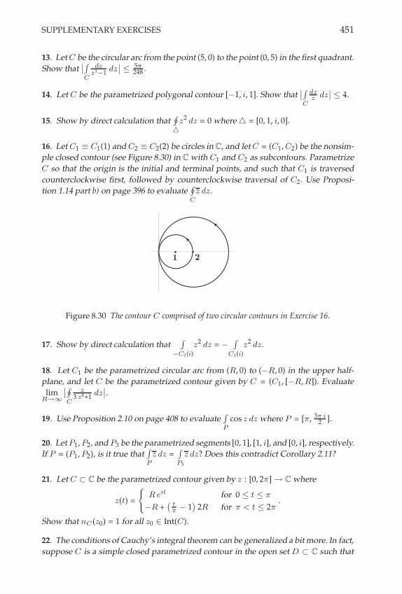
SUPPLEMENTARY EXERCISES 451
13. Let C be the circular arc from the point (5, 0) to the point (0, 5) in the first quadrant.Show that
&&Z
C
dz
z3!1 dz&& # 5#
248 .
14. Let C be the parametrized polygonal contour [&1, i, 1]. Show that&&Z
C
dz
zdz
&& # 4.
15. Show by direct calculation that]
*z
2dz = 0 where 5 = [0, 1, i, 0].
16. Let C1 . C1(1) and C2 . C2(2) be circles in C, and let C = (C1, C2) be the nonsim-ple closed contour (see Figure 8.30) in C with C1 and C2 as subcontours. ParametrizeC so that the origin is the initial and terminal points, and such that C1 is traversedcounterclockwise first, followed by counterclockwise traversal of C2. Use Proposi-tion 1.14 part b) on page 396 to evaluate
]
C
z dz.
1 2
Figure 8.30 The contour C comprised of two circular contours in Exercise 16.
17. Show by direct calculation thatZ
!C1(i)z
2dz = &
Z
C1(i)z
2dz.
18. Let C1 be the parametrized circular arc from (R, 0) to (&R, 0) in the upper half-plane, and let C be the parametrized contour given by C = (C1, [&R, R]). Evaluatelim
R&%
&&]
C
z
3 z8+1 dz&&.
19. Use Proposition 2.10 on page 408 to evaluateZ
P
cos z dz where P = [', 3# i
2 ].
20. Let P1, P2, and P3 be the parametrized segments [0, 1], [1, i], and [0, i], respectively.If P = (P1, P2), is it true that
Z
P
z dz =Z
P3
z dz? Does this contradict Corollary 2.11?
21. Let C ! C be the parametrized contour given by z : [0, 2'] , C where
z(t) =
ER e
it for 0 # t # '
&R +,
t
#& 1
-2R for ' < t # 2'
.
Show that nC (z0) = 1 for all z0 " Int(C).
22. The conditions of Cauchy’s integral theorem can be generalized a bit more. In fact,suppose C is a simple closed parametrized contour in the open set D ! C such that

452 COMPLEX INTEGRATION
Int(C) ! D, just as in Cauchy’s integral theorem. But now assume that f : D , C isdifferentiable on D \ {p} but only continuous at p for some p " C. Show that it is stilltrue that
]
C
f (z) dz = 0.
23. Show that the condition of continuity of f at p in the previous exercise can beweakened even further. One need only presume that lim
z&pf (z) exists. In fact, if p %" C,
one can presume the even weaker condition that limz&p
,(z & p) f (z)
-exists.
24. Evaluate]
C
ez
z5 dz where C is the parametrized square [2 + 2 i, &2 + 2 i, &2 & 2 i, 2 &
2 i, 2 + 2 i].
25. Let C be the ellipse given by z : [0, 2'] , C where z(t) = (3 cos t, 2 sin t). LetC1 . C 1
2(1), C2 . C 1
2(&1), C3 . C 1
2(i), and C4 . C 1
2(&i). Show that
]
C
dz
z4!1 =
;4j=1
]
Cj
dz
z4!1.
26. This and the following exercise relate to uniformly convergent sequences of com-plex functions and the interchanging of limit operations. Let fn : D , C for n =1, 2, . . ., be a sequence of functions continuous on the open set D ! C, such that {fn}converges uniformly to f : D , C on D. Show that for any parametrized contourC ! D,
limn&%
2Y
C
fn(z) dz
3=
Y
C
f (z) dz.
To do so, let C be a parametrized contour in D, and considerZ
C
,fn(z)&f (z)
-dz along
with Proposition 1.16 on page 398.
27. Let fn : D , C for n = 1, 2, . . ., be a sequence of functions differentiable on theopen set D ! C, and suppose {fn} converges uniformly to f : D , C on D. Showthat f is differentiable on D, and that
limn&%
f#n(z) = f
#(z) on D.
To do so, establish the following:
a) Show that f is continuous on D.
b) Fix z0 " D, and let C ! D be a simple closed parametrized contour such thatInt(C) ! D. Let r . dist(z0, C), and show that for $ > 0 there exists N " N
such that n > N - |fn(z) & f (z)| <$ r
2 LCfor all z " D.
c) Note that]
C
fn(+)+!z0
d* = 2' i fn(z0) for each n = 1, 2, . . ., and show from this
n > N -&&&&]
C
(fn(+)+!z0
& f (+)+!z0
)d*
&&&& < $, and so lim
2]
C
fn(+)+!z0
d*
3=]
C
f (+)+!z0
d*.
d) Apply the assumption of part c) to the conclusion of part c) to obtain the resultthat f (z0) = 1
2# i
]
C
f (+)+!z0
d*. By Corollary 4.12 on page 436, it follows that f is
differentiable on D.

SUPPLEMENTARY EXERCISES 453
C C
Figure 8.31 Two semicircular contours for Exercise 28.
e) Show that lim f#n(z0) = f
#(z0) by noting that f#n(z0) = 1
2# i
]
C
fn(+)(+!z0)2 d*, and
f#(z0) = 1
2# i
]
C
f (+)(+!z0)2 d*.
28. Computelim
t&%
Y
[c!it,c+it]
e±z
zn+1dz where c %= 0.
Hint: Consider the semicircular contours shown in Figure 8.31.
29. Evaluate]C
dz
z2!1 where C is the contour shown in Figure 8.32.
C
C1C2
1!1
Figure 8.32 The contour for Exercise 29.
30. In this exercise, you will prove the fundamental theorem of algebra using onlytechniques of winding numbers. Start with a monic7 nonconstant polynomial F (z) =
zn + a1z
n!1 + · · · + an. Assume it vanishes nowhere. We will define the closed curve
$r parametrized by /r : [0, 2'] , C given by /r(t) = F (reit)
|F (reit)| .
a) Prove that n($0, 0) = 0.
b) Fix r > 0. Show that if r# is sufficiently close to r, then n($r% , 0) = n($r, 0). (The two
curves are very close, and their winding numbers are thus very close integers.)
c) Deduce that
n($r, 0) =
Y 2#
0
/#r(t)
/r(t)dt
is continuous. Show that it is constant.
d) Take r very large. Show that /r(t) is close to eint, where n is the degree of F (z). If
r is large enough, then n($r, 0) = n, right? (Note that the dominant term in F (z) isz
n.)
7This means that the leading coefficient is 1. Why can we assume this?

454 COMPLEX INTEGRATION
e) Deduce that n($r, 0) = n for all n, and derive a contradiction.
The above exercise is from r [Hat02], where it is a theorem (though proved using thefundamental group, not winding numbers).
31. Suppose the open connected set D is simply connected,8 i.e., for any contourC ! D and w /" D, we have nC (w) = 0.
a) Prove that any differentiable f : D , C has an antiderivative on D.
b) Let u : D2 , R be harmonic on D
2, the corresponding region to D in R2. Prove
that f (z) = (u
(x& i
(u
(yis differentiable on D (as a complex function).
c) Prove that on a simply connected open set, any harmonic function has a harmonicconjugate.
d) Prove that D ! C is simply connected if and only if every differentiable g : D ,C & {0} has a differentiable logarithm. (Cf. the Appendix for a hint.)
e) Show D ! C is simply connected if and only if every harmonic function on D2
has a harmonic conjugate. (Think of log |g(z)| for g differentiable.)
8The standard definition of a simply connected set, that (intuitively) a closed curve can bedeformed into a point within that set, can be proved to be equivalent with this one.

9TAYLOR SERIES, LAURENT SERIES, AND
THE RESIDUE CALCULUS
A good calculator does not need artificial aids.
Lao Tze
In the first section of this chapter we will develop the theory of real and com-plex power series. While such series can be defined for some of the otherspaces we have previously discussed, we will restrict our attention to themost important cases, namely R and C. For results that apply to both R andC, we will denote these fields more generally by F, and an arbitrary elementof F by ). Results that are specific to either R or C will be stated explicitly interms of either, and we will denote an element of R and an element of C bythe usual x and z, respectively. In section 2 we define the important type ofpower series known as Taylor series and develop its key properties. In sec-tion 3 we use Taylor series to characterize what it means for a function tobe analytic. In the case of a complex function defined on an open connectedset D ' C, we will see that f is analytic on D if and only if f is differen-tiable on D, a significant identification that does not hold in the case of realfunctions. We then define a kind of series representation for a function neara point at which the function is not differentiable, also called a singularity ofthe function. The resulting Laurent series is extremely useful in characterizingsuch singularities. Finally, in the last section of the chapter, we show that aparticular coefficient of the Laurent series called the residue can be exploitedin evaluating complex contour integrals of the function. This so-called residuecalculus is an extremely useful technique, even for evaluating certain real in-tegrals.
455

456 TAYLOR SERIES, LAURENT SERIES, AND THE RESIDUE CALCULUS
1 POWER SERIES
1.1 Definition, Properties, and Examples
We begin with a definition.
Definition 1.1 Consider a fixed )0 # F and constants aj # F for j ! 0. Aseries of the form '+
j=0
aj () " )0)j ,
for ) # F is called a power series centered at )0. The radius of convergenceof the power series is defined as
R / sup!|) " )0| :
'+
j=0
aj() " )0)j converges"
,
when the supremum exists. When R exists and is nonzero, the neighborhoodNR()0) is called the neighborhood of convergence.
When R = 0, the series converges only at the point ) = )0, to the value a0. Ifthe supremum fails to exist the radius of convergence is considered infinite,and we will often write R = - and refer to NR()0) even in this case. WhenR = - it is not hard to show that the series converges for all ) # F. In thecase where F = R, we sometimes refer to NR(x0) = (x0 " R, x0 + R) as theinterval of convergence rather than as the neighborhood of convergence. In thecase where F = C we may refer to the circle CR(z0) / *NR(z0) as the circle ofconvergence, whereas in the case F = R the set CR(x0) consists of the endpointsof the interval of convergence. While any power series will converge for atleast ) = )0, it is not clear from the definition alone for what other points ) # F
the series might converge. Even the definition of the radius of convergenceR only tells us (roughly) the furthest distance from )0 at which convergenceoccurs. Fortunately, the situation is not as complicated as it might otherwisebe, as the following theorem establishes.
Theorem 1.2 For any power series;'
j=0 aj () " )0)j centered at )0 with radius ofconvergence R > 0, the following all hold:
a) The series converges absolutely on NR()0).
b) The series converges uniformly on Nr()0) for every r < R.
c) The series diverges for ) $# NR()0).
Convergence or divergence of the power series at points on CR()0) must be studiedindividually.
PROOF Part c) is immediate from the definition of R. To prove a) and b),consider r < R. There exists )1 # F such that r < |)1 " )0| + R and

POWER SERIES 457
;'j=0 aj()1 " )0)j converges. Since lim
j('aj()1 " )0)j = 0, there exists M ! 0
such that|aj()1 " )0)j | + M for all j ! 0.
Now suppose ) # Nr()0). Then,
|aj () " )0)j | = |aj()1 " )0)j |&&&) " )0
)1 " )0
&&&j+ M
( r
|)1 " )0|
)jfor all j ! 0,
and since r|!1"!0|
< 1, it follows from the Weierstrass M-test that;'
j=0 aj () "
)0)j converges absolutely and uniformly on Nr()0). #
! 9.1 Show that when R = 0 the associated power series centered at #0 convergesabsolutely at #0, but diverges for # %= #0.
! 9.2 Suppose;%
j=0 aj (# & #0)j is a power series centered at #0 that converges for#1 %= #0. Show that the series converges absolutely for any # such that |#�| < |#1�|,that is, for any # " Nr(#0) where r . |#1 & #0|.
! 9.3 Show that a power series converges uniformly on any compact subset of itsneighborhood of convergence.
To see that “anything can happen“ at points lying on the circle of convergenceof a power series, consider the particular complex example of
;'j=1
1j zj . Note
that the series converges at z = "1, but it diverges at z = 1. The radius ofconvergence must be R = 1 (Why?), and so the circle of convergence in thiscase contains at least one point of convergence and one point of divergencefor the series.
! 9.4 Consider the complex power series given by;%
j=01j2 z
j . Use the ratio test to
show that R = 1, and that the series converges absolutely at every point on its circleof convergence C1(0).
! 9.5 Can you find an example of a power series that does not converge at any pointon its circle of convergence?
The following corollary to Theorem 1.2 establishes a convenient fact aboutpower series, namely, they are continuous functions on their neighborhoodsof convergence.
Corollary 1.3 A power series;'
j=0 aj () " )0)j represents a continuous functionon its neighborhood of convergence.
PROOF Fix )1 # NR()0), where R is the radius of convergence for the series.Now choose r < R so that )1 # Nr()0) ' NR()0). Let fn : NR()0) 3 F bethe continuous function defined by fn()) =
;nj=0 aj () " )0)j for n ! 1. By
the previous theorem we know that;'
j=0 aj ()")0)j converges uniformly on

458 TAYLOR SERIES, LAURENT SERIES, AND THE RESIDUE CALCULUS
Nr()0). This, along with Theorem 3.8 from Chapter 5, implies that
limn('
fn()) = limn('
n+
j=0
aj () " )0)j ='+
j=0
aj () " )0)j
is continuous at )1. Since )1 # NR()0) was arbitrary, we have that f : NR()0) 3F given by f ()) /
;'j=0 aj () " )0)j is continuous on NR()0). #
Therefore, any power series centered at )0 is a continuous function of ) onits neighborhood of convergence. This neighborhood of convergence is thefunction’s domain and can be as small as )0 itself, or as large as all of F.
Examples of Power Series
The simplest type of power series is the geometric series introduced in Chapter3, namely,
;'j=0 )j . Recall that this series diverges for |)| ! 1 and converges to
11"! for |)| < 1. This fact will be extremely useful to us in what follows, since,
as indicated in the proof of Theorem 1.2, determining those values of ) forwhich a given power series converges hinges largely on determining thosevalues of ) for which the tail of the series behaves like that of a convergentgeometric series.
Example 1.4 Since;'
j=0 zj converges for |z| < 1, we may define the func-tion f : N1(0) 3 C according to
f (z) ='+
j=0
zj .
Given the discussion above, we see that the function g : C \ {1} 3 C givenby g(z) = 1
1"z is equal to f on N1(0). That is,
f (z) ='+
j=0
zj = 1 + z + z2 + · · · =1
1 " zon N1(0).
Note that the function g is actually defined outside of N1(0) as well; we havesimply established that f (z) = g(z) on N1(0). The radius of convergence ofthe series is R = 1, and the circle of convergence is C1(0). (See Figure 9.1.) "
As the above example illustrates, a power series can sometimes be writtenas a “closed formula“ function (rather than as an infinite series). In the par-ticular example above, we say that the function g(z) = 1
1"z has power series
representation;'
j=0 zj on N1(0). For the same function g(z) = 11"z , we can also
find a power series representation centered at a different point.
Example 1.5 For g : C \ {1} 3 C given by g(z) = 11"z , we will find a power
series representation for g centered at z = i. Note that
1
1 " z=
1
1 " i " (z " i)=
1
1 " i
1
1 "z"i1"i
=1
1 " i
1
1 " w,

POWER SERIES 459
for w = z"i1"i . From this we have
1
1 " z=
1
1 " i
'+
j=0
wj =1
1 " i
'+
j=0
(z " i
1 " i
)j=
'+
j=0
( 1
1 " i
)j+1(z " i)j ,
which converges for |w| =&&& z"i
1"i
&&& < 1, i.e., for |z " i| < |1 " i| =,
2, or on
N$2(i). Note that z = 1 lies on the circle of convergence C$
2(i). (See Figure9.1 again.) "
0
1
i
N%2
(i)
N1(0)
Figure 9.1 The regions of convergence for the power series in Examples 1.4 and 1.5
From Examples 1.4 and 1.5 we see that the same function g(z) = 11"z has two
different power series representations,
1
1 " z=
'+
j=0
zj = 1 + z + z2 + · · · on N1(0),
and
1
1 " z=
1
1 " i+( 1
1 " i
)2(z " i) +
( 1
1 " i
)3(z " i)2 + · · · on N$
2(i).
In fact, g(z) = 11"z has infinitely many different power series representations
corresponding to different values of z0 $= 1.
! 9.6 Suppose f : C \ {1} , C is given by f (z) = 1z!1 . Find a power series rep-
resentation for f centered at z = 2, and determine its radius and neighborhood ofconvergence.
Other examples can be analyzed in light of the special geometric series case.In each, a function is given by a formula, and an associated power seriesis sought. The strategy is to express the given function as a multiple of thequantity 1
1"w for some function w of ), and then recognize that 11"w =
;'j=0 wj
where the series converges for |w| < 1. This will yield the radius and neigh-borhood of convergence of the derived power series representation for theoriginal function.
Example 1.6 Consider the function f : C \ {13} 3 C given by f (z) = 1
1"3z .

460 TAYLOR SERIES, LAURENT SERIES, AND THE RESIDUE CALCULUS
Note that the function is not defined at z = 13 . Letting w = 3z, we have
1
1 " 3z=
1
1 " w=
'+
j=0
wj ='+
j=0
(3z)j ='+
j=0
3jzj ,
which converges for |w| = |3z| < 1, or for |z| < 13 . Therefore the radius of
convergence is 13 , and the neighborhood of convergence is N 1
3(0). Note that
the point z = 13 lies on the circle of convergence C 1
3(0). "
! 9.7 Choose any real ! > 0. Can you find a power series having radius of conver-gence equal to !?
! 9.8 For fixed a, b " F and m " N, consider the function given by the rule f (#) =1
a!b*m . Determine the neighborhood of convergence for this function’s power seriesrepresentation centered at #0 = 0.
Example 1.7 Consider the function f : C \ {±2i} 3 C given by f (z) = 1z2+4
.
Note that the function is not defined at z = ±2i. Factoring out a 14 , and letting
w = "z2
4 , we obtain
1
z2 + 4=
1
4
1
1 "
,"
z2
4
- =1
4
1
1 " w=
1
4
'+
j=0
wj =1
4
'+
j=0
( i
2
)2jz2j ,
which converges for |w| =&&"
z2
4
&& < 1, or |z| < 2. Hence, the radius ofconvergence is R = 2, and the neighborhood of convergence is N2(0). Notethat the points ±2i lie on the circle of convergence C2(0). "
The previous examples illustrate a useful method of exploiting the behaviorof geometric series to find power series representations for certain functions.The following two results are also useful in that they provide convenientmeans for computing the radius of convergence R for a given power series.The first makes use of the ratio test, and the second makes use of the roottest. Recall that both tests are based on comparison of the given series togeometric series.
Theorem 1.8 Let;'
j=0 aj () " )0)j be a power series centered at )0 with aj $= 0for all j ! 0, and let
+ / lim&&&aj+1
aj
&&&,
when the limit exists or is -. Then there are three cases:
a) If + $= 0, then R = 1% .
b) If + = 0, then R = -.
c) If + = -, then R = 0.

POWER SERIES 461
PROOF We first consider a). Suppose + = lim&&&aj+1
aj
&&& $= 0. Then if ) $= )0 we
may apply the ratio test to obtain
limj('
&&&&aj+1() " )0)j+1
aj () " )0)j
&&&& = + |) " )0|. (9.1)
From this we see that the series converges absolutely if + |) " )0| < 1 anddiverges if + |) " )0| > 1. This shows that R = 1
% . Now consider b). In thiscase, the limit in (9.1) equals zero for all ) # F. The ratio test then yields thatthe series converges absolutely for all ) # F, i.e., R = -. Finally, consider c)and suppose ) $= )0. Then,
limj('
&&&&aj+1() " )0)j+1
aj() " )0)j
&&&& = limj('
2&&&aj+1
aj
&&& |) " )0|
3= -.
Therefore, the only case in which convergence holds is ) = )0, i.e., R = 0. #
Clearly this theorem will be well suited to power series whose aj involvefactorials. On the other hand, the following result is typically more useful forthose power series whose aj involve j-dependent powers. Note too that it isa bit more general than Theorem 1.8 in that, like the root test of Chapter 3, itdefines + in terms of a lim sup rather than a limit. Of course, in those caseswhere the limit exists, it will equal the lim sup .
Theorem 1.9 Let;'
j=0 aj () " )0)j be a power series centered at )0, and let
+ / lim sup j*|aj |,
when it exists, otherwise let + = -. Then there are three cases:
a) If + $= 0, then R = 1% .
b) If + = 0, then R = -.
c) If + = -, then R = 0.
PROOF In cases a) and b), consider that
lim sup j*|aj () " )0)j | =
(lim sup j
*|aj |
)|) " )0| = + |) " )0|.
If + $= 0 then lim sup j*|aj () " )0)j | = + |) " )0| < 1 if and only if |) " )0| < 1
% ,
and therefore R = 1% . If + = 0 then lim sup j
*|aj () " )0)j | = 0 < 1, and the se-
ries converges for all ) # F, i.e., R = -. If + = - then lim sup j*|aj () " )0)j | <
1 only if ) = )0, i.e., R = 0. #
In applying either Theorem 1.8 or Theorem 1.9, it is convenient to think of Ras the reciprocal of +, even when + = 0 or + = -.

462 TAYLOR SERIES, LAURENT SERIES, AND THE RESIDUE CALCULUS
Example 1.10 We look at several examples.
a) Consider the complex power series;'
j=0 j!zj . Applying Theorem 1.8 wecompute
+ = lim
&&&&(j + 1)!
j!
&&&& = lim(j + 1) = -,
and so R = 0. Therefore the series converges only for z = 0.
b) Consider the power series;'
j=01j zj discussed previously. Applying The-
orem 1.8 we compute+ = lim
&&&&j
j + 1
&&&& = 1,
and so we confirm that R = 1 as we had deduced earlier. Recall that z = 1and z = "1 each lie on the circle of convergence C1(0) in this case, and thatthe series converges at z = "1 while it diverges at z = 1.
c) Consider the real power series;'
j=0("j)j (x " 1)j . Applying Theorem 1.9we see that
+ = lim sup j*|aj | = lim sup j
%jj = lim sup j,
which does not exist. Therefore, + = - and so R = 0. The series convergesonly for x = 1.
d) Consider the power series;'
j=0 aj zj , with
aj =
E,12
-j for odd j ! 1,
13
-j for even j ! 2.
Then it is easy to see that limj('
j*&&aj
&& does not exist. But lim sup j*&&aj
&& = 12 ,
and therefore the radius of convergence is R = 2.
e) Recall from Chapter 3 that our definition of ex was
ex/
'+
j=0
xj
j!.
We saw then, via the ratio test, that the above series converges for every x #
R. In Chapter 4, we naturally defined the exponential function exp : R 3 R
by
exp(x) = ex/
'+
j=0
xj
j!.
From this, we might naturally define a complex function given by
f (z) ='+
j=0
zj
j!(9.2)
and expect it to be equal to the complex exponential function on its neigh-borhood of convergence. To determine the radius of convergence for this

POWER SERIES 463
complex power series, apply Theorem 1.8 to see that R = -. We might betempted at this point to conclude that the complex exponential function hasthis power series representation on all of C. Recall, though, that in Chapter 4we defined the complex exponential function as exp(z) / ez
/ ex eiy. Laterwe will show that the power series given in (9.2) is equivalent to our defini-tion from Chapter 4. "
We prove one more result in this subsection, which will be of use in whatfollows. Referred to as Abel’s theorem, it establishes that if a real power seriesconverges at the right endpoint of its interval of convergence, then the powerseries is left continuous there.
Theorem 1.11 (Abel’s Theorem)Suppose f (x) =
;'j=0 aj(x"x0)j is a real power series that converges for |x"x0| <
R. If;'
j=0 ajRj converges then lim
x((x0+R)"f (x) =
;'j=0 ajR
j .
PROOF We consider the case x0 = 0 and R = 1, and leave the general case tothe reader. Suppose
;'j=0 aj = s, let Sn(x) =
;nj=0 ajx
j , and let Sj / Sj(1) =;j
k=0 ak. Then for |x| < R = 1,
f (x)
1 " x=( '+
j=0
ajxj)( '+
j=0
xj)
='+
j=0
Sjxj ,
where the second equality above is due to Theorem 5.6 in Chapter 3. Fromthis we have, for |x| < 1,
f (x) = (1 " x)'+
j=0
Sjxj
= (1 " x)'+
j=0
,Sj " s
-xj + (1 " x)
'+
j=0
s xj
= (1 " x)'+
j=0
,Sj " s
-xj + s. (9.3)
Now note that since limj('
Sj = s, for any ! > 0 there exists N # N such that
j > N ) |Sj " s| < (2 .
Therefore, for 0 + x < 1, equality (9.3) obtains
f (x) " s = (1 " x)'+
j=0
(Sj " s)xj
= (1 " x)N+
j=0
,Sj " s
-xj + (1 " x)
'+
j=N+1
,Sj " s
-xj ,

464 TAYLOR SERIES, LAURENT SERIES, AND THE RESIDUE CALCULUS
which implies that
|f (x) " s| + |1 " x|
&&&&N+
j=0
,Sj " s
-xj
&&&& + |1 " x|
'+
j=N+1
!
2|x|j
+ |1 " x|
N+
j=0
|Sj " s| +!
2|1 " x|
1
1 " |x|
= |1 " x|
N+
j=0
|Sj " s| + (2 . (Why?) (9.4)
If we choose . / !(
2;N
j=0 |Sj " s|)"1
, we obtain from inequality (9.4) that
1 " . < x < 1 ) |f (x) " s| < !,
and the special case of the result is proved. #
! 9.9 Answer the (Why?) question in the above proof. Then prove the general case;to do so, let y = x&x0 so that f (x) =
;%j=0 aj(x&x0)j becomes f (x0 +y) =
;%j=0 ajy
j .
Then rescale by letting y = Rt. This gives f (x0 + Rt) =;%
j=0 ajRjtj .
! 9.10 What conditions need be presumed in the above theorem in order to concludethat lim
x&(x0!R)+f (x) =
;%j=0 aj (&R)j?
1.2 Manipulations of Power Series
Algebraic Manipulations of Power Series
The following results are a great convenience in manipulating power series.
Theorem 1.12 Let f ()) =;'
j=0 aj ()")0)j and g()) =;'
j=0 bj ()")0)j be powerseries having radii of convergence Rf and Rg , respectively. Then,
a) (f ± g)()) =;'
j=0 cj () " )0)j where cj = aj ± bj , and
b) (fg)()) =;'
j=0 cj () " )0)j where cj =;j
k=0 ak bj"k.
In both cases, the resulting series has radius of convergence R ! min(Rf , Rg).
PROOF We prove b) and leave the proof of a) to the reader. Since;'
j=0 aj ()"
)0)j and;'
j=0 bj () " )0)j converge absolutely on Nr()0) for r = min(Rf , Rg),it follows from Theorem 5.6 in Chapter 3 (which allows for multiplication ofinfinite series) that

POWER SERIES 465
f ())g()) =
2 '+
j=0
aj () " )0)j32 '+
j=0
bj () " )0)j3
='+
j=0
2 j+
k=0
ak () " )0)k bj"k () " )0)j"k
3
='+
j=0
2 j+
k=0
ak bj"k
3() " )0)j
/
'+
j=0
cj () " )0)j , where cj /
j+
k=0
akbj"k,
and since this series converges on Nr()0) where r = min(Rf , Rg), it followsthat the radius of convergence R satisfies R ! r. #
! 9.11 Prove part 1 of the above theorem.
Theorem 1.13 Let f ()) =;'
j=0 aj () " )0)j be a power series having radius ofconvergence R. If a0 $= 0, then there exists r > 0 such that on Nr()0) we have
1
f ())=
'+
j=0
bj () " )0)j ,
whereb0 =
1
a0, and bj = "
1
a0
j+
k=1
akbj"k for j ! 1.
PROOF 1 If there is such a series;'
j=0 bj () " )0)j , then
1 =( '+
j=0
aj () " )0)j)( '+
j=0
bj () " )0)j)
='+
j=0
( j+
k=0
ak () " )0)k bj"k () " )0)j"k)
='+
j=0
( j+
k=0
ak bj"k
)() " )0)j .
This implies that a0b0 = 1, and;j
k=0 ak bj"k = 0 for j ! 1, i.e., that b0 = 1a0
and bj = "1a0
;jk=0 akbj"k for j ! 1. We must now prove that
;'j=0 bj () "
)0)j has a positive radius of convergence. Since;'
j=0 aj () " )0)j converges
1We follow [Ful78] in the proof.

466 TAYLOR SERIES, LAURENT SERIES, AND THE RESIDUE CALCULUS
for |) " )0| < R, choose 0 < r < R such that;'
j=0 aj rj converges. This
implies there exists M ! 1 such that |aj rj| + M |a0| for all j ! 0, i.e.,
|aj | +M |a0|
rjfor all j ! 0.
Now,
|b0| =1
|a0|+
M
|a0|,
|b1| =1
|a0||a1b0| +
1
|a0|
(M |a0|
r
) 1
|a0|=
1
|a0|
(M
r
),
|b2| =1
|a0||a1b1 + a2b0| +
1
|a0|
(M |a0|
r
M
|a0|r+
M |a0|
r2
M
|a0|
)=
2
|a0|
(M
r
)2,
and by induction it can be shown that
|bj | +2j"1
|a0|
(M
r
)jfor j ! 1. (9.5)
This implies
lim sup j*|bj | + lim sup
1j%
2 |a0|
(2M
r
)=
2M
r,
and therefore,
R =1
lim sup j%|bj |
!
r
2M> 0.
#
! 9.12 Use induction to prove inequality (9.5) for j ' 1.
! 9.13 Show that the coefficients bj described in Theorem 1.13 may be determinedby the “long division“ algorithm as illustrated in Figure 9.2. That is, divide 1 by thepower series representation for f (z), i.e., by a0 + a1z + a2z
2 + · · · .
a0 + a1z + a2z2+ . . .
1 + a!10 a1za!1
0 a2z2
1 + a!10 a1z + a!1
0 a2z2+ . . .
!a!10 a1z ! a!2
0 a21z
2+ . . .
a!10 ! a!2
0 a1z + . . .
!a!10 a1z ! a!2
0 a21z
2+ . . .
...
Figure 9.2 The ”long division” algorithm one can use to find the reciprocal of a power series.
Example 1.14 Suppose f : C 3 C is given by f (z) = 1 + z2. Then f is itsown power series representation on all of C. Let g : C \ {±i} 3 C be givenby g(z) = 1
f (z) = 11+z2 . Note that f (z) $= 0 on N1(0). According to the above
theorem, g(z) has a power series representation on Nr(0) for some r > 0given by

POWER SERIES 467
g(z) =1
f (z)=
'+
j=0
bj zj ,
whereb0 = 1,
b1 = "
1
a0(a1b0) = 0,
b2 = "
1
a0(a1b1 + a2b0) = "1,
b3 = "
1
a0(a1b2 + a2b1 + a3b0) = 0,
b4 = "
1
a0(a1b3 + a2b2 + a3b1 + a4b0) = 1,
etc.,
i.e.,g(z) =
1
f (z)=
1
1 + z2 = 1 " z2 + z4" z6 + · · · , on Nr(0).
The reader should verify that this power series representation for g has ra-dius of convergence R = 1. This is the same conclusion as that based onconvergent geometric series, namely,
1
1 + z2=
'+
j=0
("z2)j ='+
j=0
("1)j z2j on N1(0)."
! 9.14 Verify that the derived power series representation for g in the above examplehas radius of convergence R = 1 as claimed.
! 9.15 Find the first several terms of the power series representation for f (z) = sec z
centered at z0 = 0 using the method described in the previous exercise.
Corollary 1.15 Let f ()) =;'
j=0 aj () " )0)j and g()) =;'
j=0 cj () " )0)j bepower series each having radius of convergence Rf and Rg , respectively. If a0 $= 0,
then for some positive r < min(Rf , Rg), g(!)f (!) has power series representation
g())
f ())=
'+
j=0
2j () " )0)j on Nr()0),
with2j =
j+
k=0
ck bj"k,
where
b0 =1
a0, and bj = "
1
a0
j+
k=1
akbj"k for j ! 1
as described in Theorem 1.13.

468 TAYLOR SERIES, LAURENT SERIES, AND THE RESIDUE CALCULUS
! 9.16 Prove the above corollary and show via “long division“ that the coefficients/j are as claimed in the above theorem.
! 9.17 Find the first four terms of the Taylor series representation centered at z0 = 0for the complex function h(z) = z+1
z!1 on the neighborhood N1(0).
Term-by-Term Differentiation of Power Series
We have already seen that any power series;'
j=0 aj () " )0)j represents acontinuous function on its neighborhood of convergence. We will now show,in fact, that any power series represents a differentiable function on its neigh-borhood of convergence.
Theorem 1.16 The power series;'
j=0 aj () " )0)j with radius of convergence Ris infinitely differentiable at every ) # NR()0), and its nth derivative for n ! 1 isthe power series given by
dn
d)n
'+
j=0
aj () " )0)j ='+
j=n
j (j " 1) · · · (j " (n " 1)) aj () " )0)j"n,
i.e., the power series can be differentiated term-by-term. The differentiated powerseries has the same neighborhood of convergence as the original power series.
PROOF Suppose;'
j=0 aj (z " z0)j has radius of convergence R > 0 and fixz1 # NR(z0). We will show that
d
dz
&&&&z1
2 '+
j=0
aj(z " z0)j3
='+
j=1
j aj(z1 " z0)j"1.
We begin by choosing r such that |z1 " z0| < r < R, and recalling that;'j=0 aj(z " z0)j converges uniformly on Nr(z0). This means that Sn(z) /
;nj=0 aj(z " z0)j converges uniformly to S(z) /
;'j=0 aj (z " z0)j on Nr(z0).
By Theorem 5.3 of section 5 in Chapter 8, we know that S(z) is differentiable,and for all z # Nr(z0),
d
dz
2 '+
j=0
aj (z " z0)j3
=d
dz
(lim
n('Sn(z)
)
= limn('
( d
dzSn(z)
)
= limn('
n+
j=1
j aj (z " z0)j"1
='+
j=1
j aj(z " z0)j"1.

POWER SERIES 469
Finally note that if we are to consider the real power series;'
j=0 aj (x " x0)j ,we may “complexify“ the series and use the result proved above to obtain
d
dz
2 '+
j=0
aj(z " x0)j3
='+
j=1
j aj (z " x0)j"1. (9.6)
Now replace z in (9.6) with x to obtain
d
dx
2 '+
j=0
aj (x " x0)j3
='+
j=1
j aj(x " x0)j"1.
Extending this result to the case of higher-order derivatives, and the proofthat the differentiated series has the same radius of convergence are left tothe reader. #
! 9.18 Complete the proof of the above theorem by extending the result to higher-order derivatives. Also, show that the original power series and its claimed derivativehave the same radius of convergence by applying Theorem 1.9 on page 461.
Theorem 1.16 is a very practical result. It says that for a function given as apower series, the function is differentiable inside its associated power seriesrepresentation’s neighborhood of convergence, and the derivative is foundby differentiating the power series “term-by-term.“
Example 1.17 We have seen that the power series representation of the func-tion g(z) = 1
1"z is given by1
1 " z=
'+
j=0
zj on N1(0).
By Theorem 1.16, the derivative dgdz = 1
(1"z)2 has power series representation
given by1
(1 " z)2=
d
dz
'+
j=0
zj ='+
j=0
d
dzzj =
'+
j=1
jzj"1 on N1(0).
By differentiating again, we obtain a power series representation for d2gdz2 =
2(1"z)3 , namely,
2
(1 " z)3=
'+
j=2
j (j " 1) zj"2 on N1(0).
Clearly, there is no limit to the number of times one can differentiate a powerseries in this way. Note too that the above obtains a power series representa-tion for 1
(1"z)3 , namely,
1
(1 " z)3=
1
2
'+
j=2
j (j " 1) zj"2 on N1(0)."

470 TAYLOR SERIES, LAURENT SERIES, AND THE RESIDUE CALCULUS
Term-by-Term Integration of Power Series
In our consideration of the integration of power series, we will handle thereal and complex cases separately. Focusing on the real case first, we willshow that under the right conditions, a power series can be integrated term-by-term.
Recall from Chapter 7 that if {fn} is a sequence of integrable functions fn :[a, b] 3 R for n ! 1, such that lim
n('fn(x) = f (x) uniformly on [a, b] for some
f : [a, b] 3 R, then f is integrable on [a, b] and
limn('
Y b
afn(x) dx =
Y b
alim
n('fn(x) dx =
Y b
af (x) dx. (9.7)
Now consider a real power series;'
j=0 aj (x " x0)j with neighborhood ofconvergence NR(x0). Then by Theorem 1.2 on page 456, we know that thisseries converges uniformly on every closed interval [a, b] ' NR(x0). Lettingfn : [a, b] 3 R be defined by fn(x) /
;nj=0 aj (x " x0)j for n ! 0, we have
a uniformly convergent sequence of functions {fn} on [a, b] to f : [a, b] 3 R
where f (x) /;'
j=0 aj (x " x0)j . Subbing into (9.7), we obtain
limn('
Y b
a
2 n+
j=0
aj (x " x0)j3
dx =
Y b
a
2 '+
j=0
aj (x " x0)j3
dx. (9.8)
Since the left-hand side of the above equality involves an integral of a finitesum, we may interchange summation and integration and then take the limitto obtain '+
j=0
2Y b
aaj (x " x0)j dx
3.
Overall then, (9.8) and the above yieldY b
a
2 '+
j=0
aj (x " x0)j3
dx ='+
j=0
2Y b
aaj (x " x0)j dx
3. (9.9)
Equality (9.9) says that the series can be integrated term-by-term. We haveproved the following theorem.
Theorem 1.18 The real power series;'
j=0 aj (x" x0)j with neighborhood of con-vergence NR(x0) is integrable over any closed interval [a, b] ' NR(x0), and theintegral is given by
Y b
a
2 '+
j=0
aj (x " x0)j3
dx ='+
j=0
2Y b
aaj (x " x0)j dx
3,
i.e., the power series can be integrated term-by-term.

POWER SERIES 471
Example 1.19 Consider the function f : R 3 R given by f (x) = 11+x2 . It has
power series representation given by
1
1 + x2=
'+
j=0
("x2)j ='+
j=0
("1)j x2j ,
with neighborhood of convergence N1(0). For any ! > 0 we have [0, 1 " !] 'N1(0), and so
Y 1"(
0
1
1 + x2 dx =
Y 1"(
0
2 '+
j=0
("1)j x2j
3dx
='+
j=0
("1)j2Y 1"(
0x2j dx
3
='+
j=0
("1)j(1 " !)2j+1
2j + 1.
But we also haveY 1"(
0
1
1 + x2dx = tan"1 x
&&&&(1"()
0= tan"1(1 " !),
and so overall we obtain
tan"1(1 " !) ='+
j=0
("1)j(1 " !)2j+1
2j + 1. (9.10)
Applying Abel’s theorem on page 463, we may take the limit as ! 3 0+ in
(9.10). This yields tan"1(1) = $4 on the left-hand side and
;'j=0
("1)j
2j+1 on theright-hand side, obtaining what is known as the Leibniz series,
%
4=
'+
j=0
("1)j
2j + 1.
Multiplying the above equality by 4 obtains what is referred to as the Leibnizformula for %,
% = 4,1 "
13 + 1
5 "17 + · · ·
-. "
Example 1.20 In this example we will find a power series centered at x0 = 1and convergent on N1(1) = (0, 2) for the real natural logarithm ln x. To do so,we will exploit term-by-term integration of power series. Note that since
1
x=
1
1 " (1 " x)=
'+
j=0
(1 " x)j

472 TAYLOR SERIES, LAURENT SERIES, AND THE RESIDUE CALCULUS
converges on N1(1), it follows from Theorem 1.18 that for 0 < x < 2,
ln x =
Y x
1
1
ydy
=
Y x
1
'+
j=0
(1 " y)j dy
='+
j=0
2Y x
1(1 " y)j dy
3
='+
j=0
("1)j
j + 1(x " 1)j+1 for 0 < x < 2. (9.11)
"
! 9.19 From the results of the previous example, justify letting x , 2! to show that
ln 2 =;%
j=0(!1)j
j+1 .
We now develop a term-by-term integration theorem for complex integralsof complex power series. We will need the following result, analogous toTheorem 3.10 in Chapter 7.
Theorem 1.21 For each n # N, let fn : D 3 C be a continuous function onD and suppose there exists a function f : D 3 C such that lim
n('fn(z) = f (z)
uniformly on D. Then for any contour C ' D,
limn('
Y
C
fn(z) dz =
Y
C
limn('
fn(z) dz =
Y
C
f (z) dz.
PROOF Since each fn for n ! 1 is continuous on D, it follows from Theo-rem 3.8 in Chapter 5 that f is continuous on D. Let LC be the length of thecontour C, and let ! > 0. Then there exists N # N such that for all z # D,
n > N ) |fn(z) " f (z)| <!
2LC.
Note that
n > N )
&&&&&
Y
C
fn(z) dz "
Y
C
f (z) dz
&&&&& =
&&&&&
Y
C
,fn(z) " f (z)
-dz
&&&&& +!
2LCLC < !.
Therefore, limn('
Z
C
fn(z) dz =Z
C
f (z) dz. #
We now apply this theorem to prove the following term-by-term integrationtheorem for complex power series.

TAYLOR SERIES 473
Theorem 1.22 Let;'
j=0 aj (z"z0)j be a complex power series with neighborhoodof convergence NR(z0). Then for any contour C ' NR(z0),
Y
C
2 '+
j=0
aj (z " z0)j3
dz ='+
j=0
2Y
C
aj (z " z0)j dz
3,
i.e., the power series can be integrated term-by-term.
PROOF Let;'
j=0 aj (z " z0)j be a power series with neighborhood of con-vergence NR(z0). This series is a continuous function on NR(z0), and so itis continuous on C. Also, the series converges uniformly on Nr(z0) for allr < R, and there exists r > 0 such that r < R and C ' Nr(z0). Since the series;n
j=0 aj (z"z0)j converges uniformly to;'
j=0 aj (z"z0)j on Nr(z0), Theorem1.21 implies
Y
C
2 '+
j=0
aj (z " z0)j3
dz ='+
j=0
2Y
C
aj (z " z0)j dz
3,
and the theorem is proved. #
Example 1.23 Let C be any contour in N1(0) and consider the integralZ
C
11"z dz.
Recall that 11"z =
;'j=0 zj on N1(0), so that Theorem 1.22 obtains
Y
C
dz
1 " z=
Y
C
2 '+
j=0
zj
3dz =
'+
j=0
2Y
C
zj dz
3.
If C is parametrized by z(t) for a + t + b, this yields
Y
C
dz
1 " z=
'+
j=0
2Y
C
zj dz
3=
'+
j=0
,z(b)
-j+1"
,z(a)
-j+1
j + 1. (Why?)
"
2 TAYLOR SERIES
We now develop the theory of Taylor series expansions for real and complexfunctions. A Taylor series expansion (also referred to as a Taylor series represen-tation) of a function f centered at a point )0 is a special kind of power seriesuniquely determined by f and )0. To motivate the idea, suppose a functionf is infinitely differentiable at )0 and also suppose that f has a power seriesrepresentation on NR()0) given by
f ()) ='+
j=0
aj() " )0)j .

474 TAYLOR SERIES, LAURENT SERIES, AND THE RESIDUE CALCULUS
Evaluating the series at )0, we see that a0 = f ()0). If we now differentiate theseries we obtain f &()) =
;'j=1 jaj() " )0)j"1, and evaluating the differenti-
ated series at )0 then obtains a1 = f &()0). Differentiating the series again and
evaluating at )0 once more obtains a2 = f !!(!0)2! , and more generally we have
aj =f (j)()0)
j!for j ! 0. (9.12)
From this we see that if f is infinitely differentiable at )0 and if f has a powerseries representation there, then that power series representation is uniquesince its coefficients must be those given by (9.12). For ) # NR()0), the neigh-borhood of convergence of the series, we will investigate the significance ofthe series and its relation to the defining function f . We now formally definethis unique power series associated with f at )0 as the Taylor series of f centeredat )0.
Definition 2.1 Suppose f : D 3 F is infinitely differentiable at )0 # D ' F.Then the Taylor series of f centered at )0 is defined to be the power seriesgiven by '+
j=0
f (j)()0)
j!() " )0)j . (9.13)
The above definition says nothing about where the Taylor series of f cen-tered at )0 converges. Of course, it must converge at ) = )0 (to f ()0) in fact),but where else might it converge? If it converges at some other ) # D, isit necessarily true that it converges to the value f ()) there? Taylor’s theoremanswers these questions. Since there are significant differences in the real andcomplex cases, we will state Taylor’s theorem separately for each.
In the real case, we can appeal to Taylor’s theorem with remainder fromChapter 6. Recall from this result that if f : Nr(x0) 3 R has n + 1 deriva-tives on Nr(x0), then
f (x) =n+
j=0
f (j)(x0)
j!(x " x0)j + Rn(x) on Nr(x0), (9.14)
where Rn(x) / f (n+1)(c)(n+1)! (x " x0)n+1 for some c between x0 and x. Suppose in
addition we know that f is C' on Nr(x0) (not just at x0) and that limn('
Rn(x) =
0 on Nr(x0). Then, taking the limit as n 3 - in (9.14) obtains
f (x) ='+
j=0
f (j)(x0)
j!(x " x0)j on Nr(x0),
i.e., the Taylor series of f centered at x0 converges at each x # Nr(x0), and itconverges to the value f (x). This is the basis for referring to a Taylor series

TAYLOR SERIES 475
expansion of a function f centered at a point )0 as a Taylor series representationof f centered at that point. We have established the following result.
Theorem 2.2 (Taylor’s Theorem for Real Functions)Let f : D1
3 R be C' on some neighborhood Nr(x0) ' D1, and supposelim
n('Rn(x) = 0 on Nr(x0). Then f has unique Taylor series representation on
Nr(x0) given by
f (x) ='+
j=0
f (j)(x0)
j!(x " x0)j .
! 9.20 Prove the uniqueness in the above theorem.
While the real case of Taylor’s theorem above followed relatively easily fromTaylor’s theorem with remainder from Chapter 6, the version of Taylor’s the-orem for complex functions requires a bit more work. In fact, its proof willrequire key results from our development of complex integration.
Theorem 2.3 (Taylor’s Theorem for Complex Functions)Let f : D 3 C be differentiable on some neighborhood Nr(z0) ' D. Then f hasunique Taylor series representation on Nr(z0) given by
f (z) ='+
j=0
f (j)(z0)
j!(z " z0)j .
Before proving the complex version of Taylor’s theorem, we point out howit differs from the real one. Note that in the complex case we require onlythat f be differentiable on Nr(z0), since this will imply f is infinitely differ-entiable on Nr(z0). Also note in the complex case that we make no referenceto a Taylor remainder. It will turn out that in the complex case the remain-der will always go to zero as the degree of the associated Taylor polynomialgoes to -, and so we need not include it in the conditions of the theorem.These are two significant ways in which the complex case differs from thereal, and they point to just how restrictive it is for a complex function to bedifferentiable.
PROOF Without loss of generality, we may assume that z0 = 0 for the pur-poses of the proof. Fix z # Nr(0). Let Cs / Cs(0) be a circle of radius s < rcentered at 0 such that z # Int(Cs). Then Cauchy’s integral formula yields
f (z) =1
2%i
\
Cs
f (0)
0 " zd0. (9.15)

476 TAYLOR SERIES, LAURENT SERIES, AND THE RESIDUE CALCULUS
Now,
1
0 " z=
1
0
C1
1 "z/
D
=1
0
21 +
(z
0
)+(z
0
)2+ . . .
3by geometric series,
=1
0
C
1 +(z
0
)+(z
0
)2+ · · · +
(z
0
)N+(z
0
)N+1 1
1 "z/
D
. (Why?)
Multiplying this result by f (0) obtains
f (0)
0 " z=
N+
j=0
zj f (0)
0j+1+
2z
0
3N+1f (0)
0 " z.
Subbing this back into expression (9.15) yields
f (z) =1
2%i
\
Cs
N+
j=0
zj f (0)
0j+1d0 +
1
2%i
\
Cs
2z
0
3N+1f (0)
0 " zd0
=N+
j=0
zj 1
2%i
\
Cs
f (0)
0j+1d0 +
1
2%i
\
Cs
2z
0
3N+1f (0)
0 " zd0
=N+
j=0
zj f (j)(0)
j!+
1
2%i
\
Cs
2z
0
3N+1f (0)
0 " zd0. (9.16)
Note here that we have a version of Taylor’s theorem with remainder forcomplex functions, in that (9.16) is equivalent to
f (z) =N+
j=0
f (j)(0)
j!zj + GRN (z), (9.17)
where
GRN (z) /1
2%i
\
Cs
2z
0
3N+1f (0)
0 " zd0. (9.18)
We will now show that it is always the case that limN('
GRN (z) = 0, yielding the
result we seek. To see this, note that for 0 on Cs there exists M > 0 such that

TAYLOR SERIES 477
|f (0)| + M (Why?), and so
&&& GRN (z)&&& =
&&&&&&&
1
2%i
\
Cs
2z
0
3N+1f (0)
0 " zd0
&&&&&&&
+
1
2%
2|z|
s
3N+1 M
s " |z|2%s
=
2|z|
s
3N+1 Ms
s " |z|,
which goes to zero as N 3 - since |z| < s. Taking the limit as N 3 - in(9.17) then yields
f (z) ='+
j=0
f (j)(0)
j!zj .
Since z # Nr(0) was arbitrarily chosen, the result holds on all of Nr(0). Theuniqueness follows from the argument that began this section. #
Note that in Theorems 2.2 and 2.3 the neighborhood Nr()0) on which eachseries is shown to converge is not necessarily the whole neighborhood ofconvergence NR()0) for the series where R is the series’ radius of conver-gence. In general, Nr()0) ' NR()0). Of course, the series actually convergeson all of NR()0), and so it is customary to take r as large as one can so thatNr()0) ' D and the conditions of the theorem are satisfied.
Example 2.4 Recall in Chapter 6 we had considered the real function f :R 3 R given by f (x) = sin x with x0 = 0. We saw there that
sin x = x "
x3
3!+
x5
5!" · · · +
("1)nx2n+1
(2n + 1)!+ R2n+1(x),
where R2n+1(x) = (± sin c) x2n+2
(2n+2)! for some real number c between 0 and x.Since f (x) = sin x is C' on R and lim
n('R2n+1(x) = 0 for all x # R, it follows
from Taylor’s theorem for real functions that
sin x ='+
j=0
("1)jx2j+1
(2j + 1)!on R.
Therefore, sin x is equal to its Taylor series for every x # R. "
! 9.21 Show that the complex sine function has a Taylor series representation cen-tered at z0 = 0 of the same form as the real sine function.
Example 2.5 Consider the function f : C 3 C given by f (z) = cos z, dif-ferentiable on C. We will find the Taylor series centered at z0 = 0. Notethat f (2j+1)(0) = 0 for all j ! 0, and so the Taylor series of the even func-tion cos z will consist of only even powers of z. It is not hard to see that

478 TAYLOR SERIES, LAURENT SERIES, AND THE RESIDUE CALCULUS
f &&(z) = " cos z, f (4)(z) = cos z, and in general f (2j)(z) = ("1)j cos z for j ! 0.Therefore, f (2j)(0) = ("1)j for j ! 0, which yields a Taylor series centered atz0 = 0 for cos z of
cos z = 1 "
z2
2!+
z4
4!" · · · =
'+
j=0
("1)j
(2j)!z2j on C.
Note that this Taylor series has the same form as that of the real cosine func-tion f (x) = cos x. "
! 9.22 Find the Taylor series for f (z) = cos z centered at z0 = #
2 .
! 9.23 Show that the real cosine function has a Taylor series centered at x0 = 0 of thesame form as the complex cosine function.
Example 2.6 Consider the complex exponential function f (z) = ez , differen-tiable on C. Since f (j)(z) = ez for each j ! 0 (as derived from the definitionez
/ exeiy), we have that f (j)(0) = 1 for all j ! 0 and so the Taylor series off (z) = ez centered at z0 = 0 is
ez ='+
j=0
1
j!zj on C.
Note that this Taylor series has the same form as that of the real exponentialfunction f (x) = exp(x). Also, compare this result to that of part e) in Example1.10 on page 462. This result establishes that the complex exponential func-tion has a power series representation on its entire domain of the same formas the real exponential function. "
The careful reader might have noted that the previous three examples andtheir associated exercises hint at an interesting and useful technique. Ordi-narily, in investigating convergence of a real Taylor series for a real func-tion f (x), one must consider whether and where the remainder Rn(x) goesto zero; that is, unless the real function is a restriction of some differentiable com-plex function to the real line. In such a case, one may determine a Taylor seriesrepresentation for the “complexified“ version of the function f (z). One canthen obtain the corresponding Taylor series representation for the originalreal function by setting z = x in the complex Taylor series representation.This way, no remainders need be considered.
Example 2.7 Suppose one wishes to find a Taylor series for the real naturallogarithm centered at x0 = 1. Instead, consider the principal branch of thecomplex logarithm (restricted to C \ ("-, 0]) and find a Taylor series for itcentered at z0 = 1. Recall that Logz is differentiable on C \ ("-, 0], and so itis differentiable on a neighborhood Nr(1) of z0 = 1. Also, d
dz Logz = 1z . From
this it follows that
dj
dzjLogz =
("1)j"1(j " 1)!
zjfor j ! 1 on Nr(1),

TAYLOR SERIES 479
and so we obtain the Taylor series,
Logz ='+
j=0
("1)j
j + 1(z " 1)j+1 on Nr(1).
We leave it to the reader to show that this series has neighborhood of con-vergence N1(1). It must therefore converge for z = x # N1(1), that is, we mayconclude that the real function ln : (0,-) 3 R has Taylor series centered atx0 = 1 given by
ln x ='+
j=0
("1)j
j + 1(x " 1)j+1,
convergent on N1(1) = (0, 2) in R. Note that this agrees with our result fromExample 1.20 on page 471. "
! 9.24 Show that the complex Taylor series centered at z0 = 1 for Logz has neigh-borhood of convergence N1(1).
In the following example we see yet another interesting way in which a com-plex Taylor series can shed some light on the corresponding real version.
Example 2.8 Consider the real function f : R 3 R where f (x) = 14+x2 is
defined on the whole real line. We might expect that the Taylor series of thisfunction centered at any x0 would converge on all of R, but this is not true!In fact, for x0 = 0 we obtain the Taylor series
1
4 + x2=
'+
j=0
("1)j
4j+1x2j
with neighborhood of convergence N2(0) = ("2, 2) in R. (The reader shouldconfirm this.) Why is that? To understand what happens here, consider thecorresponding complex function 1
4+z2 studied in Example 1.7 on page 460. It’sdomain consists of C \ {±2i}, and its Taylor series expansion centered at z0 =
0 is given by 14+z2 =
;'j=0
("1)j
4j+1 z2j with neighborhood of convergence N2(0)in C. The bounded neighborhood of convergence suddenly makes sense. Thecomplex version of the function can’t include the points ±2i in the complexplane, although this limitation was not evident in the real case. The corre-sponding real Taylor series, a special case of the complex one with z = x,must conform to this limitation too! "
One can go from the real Taylor series to the corresponding complex oneas well. For example, as we saw in Example 2.4 on page 477, the real sine
function has a real Taylor series sin x =;'
j=0("1)j
(2j+1)!x2j+1 that is convergent
on all of R. This allows us to conclude that the complex Taylor series given
by F (z) =;'
j=0("1)j
(2j+1)!z2j+1 converges on all of C and equals sin x when z = x.
In fact, it must equal sin z for all z # C. To see this, apply Taylor’s theorem

480 TAYLOR SERIES, LAURENT SERIES, AND THE RESIDUE CALCULUS
for complex functions to sin z centered at z = 0. Since sin z and all of itsderivatives evaluated at the origin must match those of sin x, the Taylor seriesrepresentation of the complex sine function centered at the origin must havethe same form as the Taylor series representation of the real sine functioncentered at the origin. Hence the complex version must converge for all realz. If it didn’t converge at some z1 # C, a contradiction would result.
! 9.25 Derive the contradiction that would result from the above argument. Also,in the above discussion, does it matter whether the Taylor series representations forthe real and complex sine functions are centered at the origin? What if they were bothcentered at some other real value x0? What if the complex series is centered at someother z0 " C?
We give one more example of interest.
Example 2.9 For c # C fixed, consider the function f : N1(0) 3 C written asf (z) = (1 + z)c and defined as
f (z) = (1 + z)c / exp(c Log(1 + z)). (9.19)
Then f is a differentiable function in the open unit disk. In fact, the chain ruleapplied to (9.19) obtains f &(z) = c(1 + z)c"1, and by induction it follows thatf (n)(0) = c(c " 1) . . . (c " (n " 1)). If we define the binomial coefficient
,ck
-by2
c
k
3/
c(c " 1) . . . (c " (k " 1))
k!,
then Taylor’s theorem for complex functions yields
(1 + z)c = 1 +
2c
1
3z +
2c
2
3z2 + · · · =
'+
j=0
2c
j
3zj if |z| < 1. (9.20)
"
! 9.26 Use induction to show that f(n)(0) = c(c & 1) . . . (c & (n & 1)) for n ' 1.
! 9.27 Show directly that the radius of convergence of the series in (9.20) is 1 exceptin one important case. What is that case?
! 9.28 Show that the series in (9.20) gives the ordinary binomial theorem if c is apositive integer.
It is worth pointing out that we usually don’t compute the Taylor seriescoefficients for a given function f ()) by direct application of the formula
aj = f (j)(!0)j! given in expression (9.13) of Definition 2.1. Instead, we exploit
the uniqueness of the Taylor series representation for a given function f cen-tered at a particular point.
Example 2.10 We have already seen that the function given by f (z) = 11"z
has power series;'
j=0 zj centered at z0 = 0 with neighborhood of conver-gence N1(0). Since the Taylor series representation of f is unique, this powerseries must be the Taylor series of f centered at z0 = 0. Each coefficient aj = 1

ANALYTIC FUNCTIONS 481
must be f (j)(z0)j! = f (j)(0)
j! , that is, f (j)(0) = j!. We leave it to the reader to verifythis. "
! 9.29 Recall that in our discussion of power series in the last section we saw thatthe function with the formula f (z) = 1
4+z2 had power series representation given
by;%
j=0(!1)j
4j+1 z2j centered at z0 = 0 and convergent on N2(0). Verify from this that
f##(0) = & 1
8 , and that fn(0) = 0 for all odd n.
! 9.30 Suppose f , g : Nr(#0) , F each have Taylor series representations on Nr(#0).
Suppose also that f(j)(#0) = g
(j)(#0) for j ' 0. Show that f (#) = g(#) on Nr(#0).
3 ANALYTIC FUNCTIONS
3.1 Definition and Basic Properties
We now define one of the most important classes of functions in analysis,especially complex analysis.
Definition 3.1 A function f : D 3 F is called analytic at )0 # D if and onlyif f has a Taylor series representation on some neighborhood Nr()0) ' D. Iff is analytic at every point ) # D, we say that f is analytic on D.
Note that according to the definition, a function is analytic at a point )0 in itsdomain only if there exists a neighborhood Nr()0) centered at )0 such that f ())equals its Taylor series expansion throughout that neighborhood, i.e.,
f ()) ='+
j=0
f (j)()0)
j!() " )0)j on Nr()0).
If a function equals its Taylor series representation only at the point )0, this isnot enough to conclude that f is analytic at )0.
Example 3.2 Since the complex function f : N1(0) 3 C given by f (z) = 11"z
has the Taylor series representation
f (z) ='+
j=0
zj on N1(0),
it is analytic at z0 = 0. Similarly, the real function f : N1(0) 3 R given byf (x) = 1
1"x is analytic at x0 = 0. "
Theorem 3.3 Suppose f : D 3 F has a Taylor series representation on someneighborhood Nr()0) ' D. Then f is analytic at each point ) # Nr()0).

482 TAYLOR SERIES, LAURENT SERIES, AND THE RESIDUE CALCULUS
! 9.31 Prove the above theorem. (Hint: Consider arbitrary #1 " Nr(#0). Choose , =12
,r & |#1 & #0|
-, and consider N)(#1). Show that f has Taylor series representation on
N)(#1).)
Example 3.4 From the above result we see that the complex function f :N1(0) 3 C in the previous example given by f (z) = 1
1"z is analytic on N1(0).
Likewise, the real function f : N1(0) 3 R given by f (x) = 11"x is analytic on
N1(0) = ("1, 1). "
Clearly if f is analytic at )0, it is infinitely differentiable there. But infinitedifferentiability alone is not enough to ensure analyticity, at least not for realfunctions. In fact, the following example illustrates that a real function canbe infinitely differentiable and even have a Taylor series representation at apoint, and yet not be analytic there.
Example 3.5 Consider the function f : R 3 R given by
f (x) =
Eexp("1/x2) for x $= 0
0 for x = 0.
We will show that this function has a Taylor series centered at x0 = 0 thatconverges for all x # R. Yet, this Taylor series will only equal the function’svalue at x0 = 0, and so the function is not analytic there despite being C'
there. We begin by finding the Taylor series centered at x0 = 0 for f . Notethat f (0) = 0. To find f &(0), we use the limit definition to obtain
f &(0) = limh(0
exp("1/h2)
h
= limy(±'
y
ey2 for y = 1/h,
= 0 by L’Hospital’s rule.
We leave it to the reader to show that the same strategy yields
f (j)(0) = 0 for all j ! 0,
and therefore the Taylor series for f centered at x0 = 0 is given by
'+
j=0
f (j)(0)
j!xj
/ 0.
Clearly this does not equal the function’s values at x $= 0. "
! 9.32 Show that f(j)(0) = 0 for all j ' 0 for the function f of the previous example.
It might be surprising to learn that such a function as the one in the pre-vious example exists. In fact, in the complex case such functions don’t ex-ist. As we already know, if a complex function f is differentiable at a pointit is infinitely differentiable there. In the next subsection we will discover

ANALYTIC FUNCTIONS 483
even more, namely, a complex function f is differentiable on a neighborhoodNr(z0) if and only if it is analytic on that neighborhood. Differentiable com-plex functions are very nice functions.
! 9.33 Suppose f , g : D , F are analytic at #0 " D. Show the following:
a) f ± g is analytic at #0,
b) fg is analytic at #0,
c) f/g is analytic at #0 provided g(#0) %= 0.
3.2 Complex Analytic Functions
The following proposition establishes an important and useful fact, namely,the interchangeability of the terms differentiable and analytic for complex func-tions on open connected sets D.
Proposition 3.6 Consider the complex function f : D 3 C. Then f is differen-tiable on D if and only if f is analytic on D.
! 9.34 Prove the above proposition.
! 9.35 Show that the function f : C , C given by f (z) = |z|2 is not analytic any-where in C. Is it differentiable anywhere?
As a consequence of establishing Proposition 3.6, many results stated earlierin terms of differentiable complex functions can now be restated in termsof analytic complex functions (although we will not do so). The followingexercise provides such an opportunity to the reader.
! 9.36 Show that if fn : D , C for n ' 1 is a sequence of analytic complex functionson the open connected set D ! C that converges uniformly to f : D , C on D, thenf is analytic on D.
Example 3.7 Consider the complexified version of the real function fromExample 3.5, which we saw was not analytic at the origin, even though itwas C' there. The complexified version is f : C 3 C given by
f (z) =
Eexp("1/z2) for z $= 0
0 for z = 0.
Clearly f is differentiable for z $= 0, and is therefore analytic on C \ {0}. If fwere also (complex) differentiable at z = 0 then f would be analytic there aswell, and so f would have a Taylor series representation
'+
j=0
f (j)(0)
j!zj ,
on Nr(0) for some r > 0. But this in turn would imply that for z = x, the real

484 TAYLOR SERIES, LAURENT SERIES, AND THE RESIDUE CALCULUS
version of the function would have Taylor series representation
'+
j=0
f (j)(0)
j!xj ,
on Nr(0) = ("r, r) ' R, which would imply that the real version of the func-tion was analytic at x = 0. This contradiction tells us that the complex versionof the function in this example cannot be differentiable at z = 0. In fact, onecan show that the complex version of this function isn’t even continuous atz = 0 since lim
z(0f (z) does not exist. "
! 9.37 Show that limz&0
f (z) does not exist for the function f of the above example.
Analytic functions play a particularly important role in complex function the-ory, so determining their key properties (as related to their Taylor series rep-resentation) is fundamental to any development of analysis. Loosely stated,a function that is analytic on a neighborhood behaves much like an infinite-degree polynomial there. As with polynomials, it is often useful to character-ize the zeros of analytic functions.
Zeros of Complex Analytic Functions
Recall that the fundamental theorem of algebra says that every nonzero poly-nomial with complex coefficients has at least one complex root, i.e., for poly-nomial p(z) = a0 +a1 z+· · ·+an zn, with an $= 0 and aj # C for 0 + j + n, thereexists z0 # C such that p(z0) = 0. From elementary algebra we may write
p(z) = (z " z0) q1(z),
where q1(z) is a polynomial of degree n " 1. If q1(z0) = 0, then we can write
p(z) = (z " z0)2 q2(z),
and so on, until finally we can write
p(z) = (z " z0)m q(z),
where q(z) is a polynomial such that q(z0) $= 0. In this case we say that z0 is aroot or zero of multiplicity m ! 1. We now extend these ideas to more generalcomplex functions.
Definition 3.8 Let f : D 3 C be differentiable on D. Then,
1. The point z0 is an isolated zero of f if and only if f (z0) = 0 and
f (z) $= 0 on some deleted neighborhood N &r(z0) ' D.
2. Let z0 # D be an isolated zero of f such that there exists m # Z+
with f (z) = (z " z0)m g(z), where g : D 3 C is differentiable on D
and g(z0) $= 0. Then the number m is called the multiplicity of

ANALYTIC FUNCTIONS 485
the zero of f at z0.
Note in part 2 of the above definition that since g is differentiable it is alsocontinuous. Since g is nonzero at z0 the continuity of g implies the existenceof a neighborhood Nr(z0) on which g is nonzero. In a certain sense, then, thefunction f , which has an isolated zero of multiplicity m at z0, behaves muchlike (z " z0)m near z0.
Theorem 3.9 Let f : D 3 C be differentiable on D, and let z0 # D be an iso-lated zero of f . Then there exists some integer m ! 1 such that z0 is a zero of f ofmultiplicity m.
PROOF Choose Nr(z0) ' D. By Taylor’s theorem we have
f (z) ='+
j=0
aj (z " z0)j for z # Nr(z0),
and since f (z0) = 0 it follows that we may start the series index at j = 1. Letam be the coefficient corresponding to the smallest m ! 1 such that am $= 0.Note that such an m exists, otherwise aj = 0 for all j ! 1 implying f (z) / 0on Nr(z0), which contradicts that z0 is an isolated zero of f . Since a1 = a2 =· · · = am"1 = 0, we have
f (z) ='+
j=m
aj (z " z0)j = (z " z0)mAam + am+1 (z " z0) + · · ·
Bon Nr(z0).
Let g : D 3 C be defined by
g(z) =
Ef (z)
(z"z0)m for z # D \ {z0}
am for z = z0.
Then f (z) = (z " z0)m g(z) on D, where g(z0) = am $= 0. We leave it to thereader to show that g is differentiable on D. #
! 9.38 Show that g is differentiable on D.
Suppose D ' C is open and connected. The following theorem establishesthat if f : D 3 C is a complex differentiable function that is not identicallyequal to zero on D, then the zeros of f must be isolated.
Theorem 3.10 Let f : D 3 C be differentiable on the open connected set D ' C,and let Zf ' D be the set of zeros of f in D. If Zf has a limit point in D, thenf (z) / 0 on D.

486 TAYLOR SERIES, LAURENT SERIES, AND THE RESIDUE CALCULUS
PROOF Define the set A ' D according to
A =.z # D : f (j)(z) = 0 for all j ! 0
/.
We will show that the sets A and D \ A are both open. To see that A is open,suppose z0 # A. Then for some neighborhood Nr(z0),
f (z) ='+
j=0
f (j)(z0)
j!(z " z0)j = 0 for z # Nr(z0) ' D.
This implies that Nr(z0) ' A, and therefore A is open. To show that D \ Ais open, let z0 # D \ A. Then there exists m # N such that f (m)(z0) $= 0. Bycontinuity of f (m)(z) at z0 there exists some neighborhood Nr(z0) ' D onwhich f (m)(z) is nonzero, and hence Nr(z0) ' D \A. Therefore D \A is open.Now, since D is connected and D = A % (D \ A), it follows that either A = !
or A = D. Finally, suppose Zf has a limit point z) # D. We will show thatz) # A, and therefore A = D, proving that f (z) / 0 on D. To see that z) # A,we write
f (z) ='+
j=0
f (j)(z))
j!(z " z))j for z # Nr(z)) ' D.
If z) $# A there exists a smallest m ! 0 such that f (m)(z)) $= 0. This impliesthat for some 0 < s < r,
f (z) = (z " z))m h(z) on Ns(z)) ' Nr(z)) ' D,
where h(z) $= 0 on Ns(z)). (Why?) This contradicts the fact that z) is a limitpoint of Zf . Therefore z) # A, and so A = D, completing the proof. #
! 9.39 Answer the (Why?) in the above proof.
Corollary 3.11 Suppose f , g : D 3 C are differentiable on the open connected setD ' C.
a) If f (z) = 0 for all z # A ' D where the set A has a limit point in D,
then f (z) / 0 on D.
b) If f (z) = g(z) for all z # A ' D where the set A has a limit point in D,
then f / g on D.
! 9.40 Prove the above corollary.
Part b) of the above corollary is sometimes referred to as the identity principle.
Example 3.12 We will apply the above corollary to show that 1 + tan2 z =sec2 z for all z # C. To see this, let f : C 3 C be given by f (z) = sec2 z "
tan2 z"1. Then since f (x) = sec2 x" tan2 x"1 / 0 for all x # R, the corollaryyields that f (z) / 0 for all z # C. "
! 9.41 What other trigonometric identities can be derived in this way?

LAURENT’S THEOREM FOR COMPLEX FUNCTIONS 487
4 LAURENT’S THEOREM FOR COMPLEX FUNCTIONS
Consider the function f : C \ {2} 3 C given by f (z) = 1z"2 . By Taylor’s
theorem, f has a Taylor series centered at z0 = 0 with neighborhood of con-vergence N2(0). That is,
f (z) ='+
j=0
f (j)(0)
j!zj on N2(0).
But this function f is also defined for |z| > 2, so it is natural to ask if fcan be represented by some (other) series expansion centered at z0 = 0 andconvergent for |z| > 2. To explore this, note that
f (z) =1
z " 2=
1
z
C1
1 "2z
D
=1
z
'+
j=0
(2
z
)j=
'+
j=0
2j
zj+1,
and this series converges for&& 2z
&& < 1, i.e., for |z| > 2. This type of power
series, which involves powers of 1z"z0
, or equivalently, negative powers of(z " z0), is known as a Laurent series. More generally, the form of a Laurentseries centered at a point z0 involves both positive and negative powers of(z " z0), that is,
f (z) ='+
j=0
aj (z " z0)j +'+
j=1
bj
(z " z0)j, (9.21)
and so it consists of two infinite series. The first series in (9.21) is often referredto as the analytic part and the second series in (9.21) is often referred to asthe singular part, or the principal part of the Laurent series. For the Laurentseries expansion to exist at a particular z # C, both the analytic part and thesingular part must be convergent at z. In fact, the analytic part consistingof positive powers of (z " z0) will converge for all z inside some circle ofradius R, while the singular part consisting of negative powers of (z " z0)will converge for all z outside some circle of radius r, as in our example. Itis the overlap of the two regions of convergence associated with the analyticpart and the singular part that comprises the region of convergence of theLaurent series. This region of overlap is typically the annulus centered at z0
and denoted by ARr (z0) = {z # C : r < |z " z0| < R}. See Figure 9.3 for an
illustration. The situation R = - and r = 0 corresponds to the case wherethe Laurent series converges everywhere in C except possibly at z0. (In ourparticular example, we have convergence in the annulus A'
2 (0).) Note thatsince the annulus so described excludes the point z0, it is not necessary that fbe differentiable at z0 for it to have a Laurent series expansion centered there.(In fact, the function f need not be differentiable anywhere within Nr(z0).)
If 0 < r < r1 < R1 < R we will refer to the annulus AR1r1 (z0) ' AR
r (z0)as a proper subannulus of AR
r (z0). In a manner similar to that of a convergent

488 TAYLOR SERIES, LAURENT SERIES, AND THE RESIDUE CALCULUS
z0
r R
ARr (z
0)
Figure 9.3 The region of convergence of a Laurent series.
Taylor series on subsets of its neighborhood of convergence, when a functionf has a convergent Laurent series expansion on an annulus AR
r (z0), it will
converge absolutely on ARr (z0) and uniformly on A
R1r1 (z0) where A
R1r1 (z0) is
any proper subannulus of ARr (z0). To establish this, we must consider the
convergence of a given Laurent series a bit more carefully. Since the analyticpart of the Laurent series is a power series, it will converge absolutely on itsneighborhood of convergence NR(z0). Recall that the convergence is uniformon NR1
(z0) for any 0 < R1 < R. To analyze the singular part, we define
r / inf
$|z " z0| :
'+
j=1
bj
(z " z0)jconverges
4.
If r fails to exist then the singular part never converges. If r exists then wewill show that the singular part converges absolutely for (Nr(z0))C , and uni-formly on (Nr1(z0))C for any r1 > r. To see this, choose r1 > r. Then as indi-
cated in Figure 9.4 there exists z1 such that r + |z1"z0| < r1 and;'
j=1bj
(z1"z0)j
converges. Therefore, there exists M ! 0 such that&&&&
bj
(z1 " z0)j
&&&& + M for all j ! 1.
Now, for z # (Nr1 (z0))C we have&&&&
bj
(z " z0)j
&&&& =
&&&&bj
(z1 " z0)j
&&&&
2|z1 " z0|
|z " z0|
3j
+ M
2|z1 " z0|
r1
3j
.
Since |z1"z0| < r1 this establishes via the Weierstrass M-test that;'
j=1bj
(z"z0)j
converges absolutely on (Nr(z0))C and uniformly on (Nr1(z0))C . Since r1 > rwas arbitrary, this result holds for any r1 > r. We leave it to the reader to
show that;'
j=1bj
(z"z0)jdiverges on Nr(z0). As with a Taylor series, the points
on the boundary Cr(z0) must be studied individually.

LAURENT’S THEOREM FOR COMPLEX FUNCTIONS 489
r
r1
z0
Figure 9.4 The regions of convergence and divergence of the singular part of a Laurent series.
! 9.42 As claimed above, show that;%
j=1bj
(z!z0)j diverges on Nr(z0).
The above discussion and exercise establish the following result.
Proposition 4.1 Suppose f : D 3 C has a Laurent series expansion f (z) =;'
j=0 aj(z " z0)j +;'
j=1bj
(z"z0)jon the annulus AR
r (z0) ' D (where r ! 0 and R
may be -). Then for any proper subannulus AR1r1 (z0) ' AR
r (z0) the given Laurent
series expansion for f converges absolutely on AR1r1 (z0) and uniformly on A
R1r1 (z0).
This result, in turn, implies the following. It will be instrumental in provingpart of the key result of this section.
Proposition 4.2 Let;'
j=1bj
(z"z0)jbe the singular part of a Laurent series expan-
sion for f : D 3 C on ARr (z0) ' D. Then
;'j=1
bj
(z"z0)jrepresents a continuous
function on (Nr(z0))C , and for any contour C ' (Nr(z0))C we haveY
C
2 '+
j=1
bj
(z " z0)j
3dz =
'+
j=1
Y
C
bj
(z " z0)jdz.
! 9.43 Prove the above proposition.
It is also true, and of great practical value as we will see, that when a Laurentseries expansion exists for a function it is unique. To see this, suppose f isdifferentiable on the annulus AR
r (z0) and suppose too that it has a convergentLaurent series there given by
f (z) ='+
k=0
ak(z " z0)k +'+
k=1
bk
(z " z0)k. (9.22)

490 TAYLOR SERIES, LAURENT SERIES, AND THE RESIDUE CALCULUS
Recall that we established the uniqueness of the Taylor series representationof a function centered at a point by differentiating the series term-by-term;here, we will establish the uniqueness of the Laurent series representation byintegrating term-by-term. Let C be any simple closed contour in AR
r (z0) with
nC (z0) = 1, and note that C ' AR1r1 (z0) ' AR
r (z0) for some proper subannulus
AR1r1 (z0) ' AR
r (z0). Also note that for any k ! 0,
\
C
f (0)
(0 " z0)k+1d0 =
\
C
'+
j=0
aj (0 " z0)j"k"1 d0 +
\
C
'+
j=1
bj
(0 " z0)j+k+1d0
='+
j=0
\
C
aj (0 " z0)j"k"1 d0 +'+
j=1
\
C
bj
(0 " z0)j+k+1d0 (9.23)
= 2%i ak nC (z0)
= 2%i ak.
Note in (9.23) above that the integral of each summand corresponding toaj for j $= k, and for bj for j ! 1, vanishes due to the integrand havingan antiderivative within NR1
(z0). Also, in integrating the singular part term-by-term, we have applied Proposition 4.2. This shows that each ak in (9.22)is uniquely determined by f and z0. A similar argument can be made forthe uniqueness of each bk for k ! 1 in (9.22) by considering the integral]
C
f (/)(/"z0)"k+1 d0 for any fixed k ! 1. We leave this to the reader.
! 9.44 Establish the uniqueness of the bk terms in the Laurent series representation
(9.22) by carrying out the integral]
C
f (+)(+!z0)"k+1 d* for any fixed k ' 1.
With these important facts about an existing Laurent series established, wenow state and prove Laurent’s theorem, the key result of this section. It isa kind of sibling to Taylor’s theorem in complex function theory. It givesconditions under which a function f : D 3 C is guaranteed a Laurent seriesrepresentation convergent on an annulus AR
r (z0) ' D.
Theorem 4.3 (Laurent’s Theorem)Let f : D 3 C be differentiable on the annulus AR
r (z0) = {z : r < |z " z0| < R} '
D (where r ! 0 and R may be -). Then f (z) can be expressed uniquely by
f (z) ='+
j=0
aj(z " z0)j +'+
j=1
bj
(z " z0)j,
on ARr (z0). For any choice of simple closed contour C ' AR
r (z0) with nC (z0) = 1,the coefficients aj and bj are given by
aj =1
2%i
\
C
f (0)
(0 " z0)j+1d0 for j ! 0,

LAURENT’S THEOREM FOR COMPLEX FUNCTIONS 491
and
bj =1
2%i
\
C
f (0)
(0 " z0)"j+1d0 for j ! 1.
PROOF As in the proof of Taylor’s theorem, we may assume that z0 = 0. Fixz # AR
r (0). Choose circles C1 and C2 in ARr (0) such that both are centered at
0, with radii R1 and R2, respectively, satisfying r < R2 < |z| < R1 < R.
C2
C2
0
AR1
R2 z
C3
Figure 9.5 The situation in the proof of Laurent’s theorem.
As indicated in Figure 9.5, choose a third circle C3, centered at z and havingradius R3, with R3 small enough that C3 is contained in AR
r (0) and does not
intersect C1 or C2. Then, since nC1= nC3
+ nC2on
,AR
r (0)-C
% {z} (Why?),we have
1
2%i
\
C1
f (0)
0 " zd0 =
1
2%i
\
C3
f (0)
0 " zd0 +
1
2%i
\
C2
f (0)
0 " zd0 by Theorem 3.6, Chap. 8
= f (z) +1
2%i
\
C2
f (0)
0 " zd0 by Cauchy’s formula.
Solving for f (z) gives
f (z) =1
2%i
\
C1
f (0)
0 " zd0 "
1
2%i
\
C2
f (0)
0 " zd0
=1
2%i
\
C1
f (0)
0 " zd0 +
1
2%i
\
C2
f (0)
z " 0d0. (9.24)
We will show that the first integral on the right-hand side of (9.24) leads tothe analytic part of the Laurent series expansion for f (z), while the secondintegral on the right-hand side leads to the singular part. The analysis of the

492 TAYLOR SERIES, LAURENT SERIES, AND THE RESIDUE CALCULUS
first integral proceeds just as in the proof of Taylor’s theorem, that is,
1
2%i
\
C1
f (0)
0 " zd0 =
N+
j=0
zj 1
2%i
\
C1
f (0)
0j+1d0 +
1
2%i
\
C1
2z
0
3N+1 f (0)
0 " zd0.
In this case, however, we can no longer expect that 12$i
]C1
f (/)/j+1 d0 = f (j)(0)
j! ,
because f is not necessarily differentiable inside C1. Therefore, we define aj
by aj /1
2$i
]C1
f (/)/j+1 d0, for whatever value this integral takes. This yields
1
2%i
\
C1
f (0)
0 " zd0 =
N+
j=0
ajzj +
1
2%i
\
C1
2z
0
3N+1 f (0)
0 " zd0,
and letting N 3 - as in the proof of Taylor’s theorem gives the analytic part,
1
2%i
\
C1
f (0)
0 " zd0 =
'+
j=0
ajzj .
To obtain the singular part, we apply a similar technique. Consider that for0 # C2,
f (0)
z " 0=
f (0)
z
C1
1 "/z
D
=f (0)
z
C
1 +0
z+ · · · +
(0
z
)N+(0
z
)N+1 1
1 "/z
D
= f (0)
C1
z+
0
z2+ · · · +
0N
zN+1+(0
z
)N+1 1
z " 0
D
=N+1+
j=1
0j"1
zjf (0) +
(0
z
)N+1 f (0)
z " 0,
so that,
1
2%i
\
C2
f (0)
z " 0d0 =
N+1+
j=1
1
zj
21
2%i
\
C2
0j"1f (0) d0
3+
1
2%i
\
C2
(0
z
)N+1f (0)
z " 0d0.
In this case, define bj /1
2$i
]C2
0j"1f (0) d0, and take the limit as N 3 - toobtain
1
2%i
\
C2
f (0)
z " 0d0 =
'+
j=1
bj
zj.
Finally, consider aj = 12$i
]C1
f (/)/j+1 d0. To show that the conclusion holds for
any simple closed contour C ' ARr (z0) with nC (z0) = 1, consider any such
C. Then nC = 1 on Nr(0), and also nC1= nC on
,AR
r (0)-C , obtaining via
Theorem 3.6 from Chapter 8,
aj =1
2%i
\
C1
f (0)
0j+1d0 =
1
2%i
\
C
f (0)
0j+1d0.

SINGULARITIES 493
A similar argument works to show that bj = 12$i
]C 0j"1f (0) d0. Finally, the
uniqueness of the Laurent series expansion was established prior to the state-ment of the theorem. #
! 9.45 Answer the (Why?) question in the above proof. To do so, exploit the factthat the contours are all circles, and consider the cases z, Int(Cr(0)), and Ext(CR(0))separately.
In a certain sense, the concept of the Laurent series expansion generalizesthat of the Taylor series expansion. It allows for a series representation off : D 3 C in both negative and positive powers of (z " z0) in a regionthat excludes points where f is not differentiable. In fact, if the function fis differentiable on all of NR(z0) the Laurent series will reduce to the Taylorseries of the function centered at z0.
One practical use of a function’s Laurent series representation is the charac-terization of that function’s singularities. We consider this topic next.
5 SINGULARITIES
5.1 Definitions
In our motivating example from the last section we discussed the functionf : C \ {2} 3 C given by f (z) = 1
z"2 . The point z0 = 2 is one where thefunction f fails to be differentiable, and hence no Taylor series can be foundfor f centered at z0 = 2. Yet, f is differentiable at points z arbitrarily near toz0. Such a point z0 is called a singularity of the function f .
Definition 5.1 Suppose f : D 3 C is not differentiable at z0 # C. If f isdifferentiable at some point z in every deleted neighborhood N &
r(z0), then z0
is called a singularity of f .
There are different types of singularities, and we characterize them now.First, we distinguish between isolated and nonisolated singularities.
Definition 5.2 Suppose z0 # C is a singularity of f : D 3 C. If f is differ-entiable on some deleted neighborhood N &
r(z0) ' D centered at z0, then z0
is called an isolated singularity of f . Otherwise, z0 is called a nonisolatedsingularity of f .
Example 5.3 The function f : C \ {0} 3 C given by f (z) = 1z has an isolated
singularity at z0 = 0. The function Log : C \ {0} 3 C given by Log(z) =ln |z|+ i Arg(z) has nonisolated singularities at every point z = x # ("-, 0]."

494 TAYLOR SERIES, LAURENT SERIES, AND THE RESIDUE CALCULUS
! 9.46 Consider the function f : C , C given by f (z) =
Ez if Im(z) ' 0
&z if Im(z) < 0.
Find the singularities of f and characterize them as isolated or nonisolated. What if&z is replaced by z?
While we cannot find a Taylor series centered at a singularity of f , we can al-ways find a Laurent series centered at an isolated singularity, convergent in anannulus that omits that point. The Laurent series can then be used to furthercharacterize the isolated singularity. There are three subtypes to consider. Inthe following definition, note that N &
r(z0) is an annulus Ar0(z0) centered at z0.
Definition 5.4 Let z0 be an isolated singularity of f : D 3 C, and suppose
f has Laurent series representation f (z) =;'
j=0 aj (z " z0)j +;'
j=1bj
(z"z0)jon
N &r(z0) ' D.
1. If bj = 0 for all j ! 1, then f is said to have a removable singularity
at z0.
2. If there exists N # N such that bj = 0 for j > N but bN $= 0, then f is
said to have a pole of order N at z0. In the special case where N = 1,
the pole is often referred to as a simple pole.
3. Otherwise f is said to have an essential singularity at z0.
It is not hard to show that f has an essential singularity at z0 if and only ifbj $= 0 for infinitely many values of j ! 1 in its Laurent series expansion, thatis, if the Laurent series expansion’s singular part is an infinite series.
! 9.47 Prove the above claim.
According to this definition, if z0 is an isolated singularity of f : D 3 C onecan determine what type of singularity z0 is by finding the Laurent seriesrepresentation for f on an annulus AR
r (z0) centered at z0, and scrutinizing itssingular part. However, in practice it is often difficult to obtain the Laurentseries directly via Laurent’s theorem. Finding alternative means for makingthis determination is therefore worthwhile, and we do so now. The key willbe to exploit the uniqueness of the Laurent series representation of a givenfunction on a particular annular region. The following example illustratesthe idea.
Example 5.5 Consider the function f : C \ {0} 3 C given by f (z) = 1z3 ez .
We leave it to the reader to confirm that z0 = 0 is an isolated singularity. Todetermine what type of isolated singularity z0 = 0 is we will find the Laurentseries representation of f on N &
1(0). To this end, note that f has the form f (z) =1z3 f0(z) where the function f0 is differentiable on C. Therefore, we can expand
f0 in a Taylor series centered at z0 = 0, namely, f0(z) = ez =;'
j=01j!z
j . We

SINGULARITIES 495
then can write,
f (z) =1
z3
'+
j=0
1
j!zj =
'+
j=0
1
j!zj"3 =
1
z3+
1
z2+
1
2!
1
z+
1
3!+
1
4!z +
1
5!z2 + · · ·
which is convergent on A'0 (0). By the uniqueness property of Laurent series
representations, this must be the Laurent series centered at z0 = 0 for f . Sinceb3 = 1, and bn = 0 for n ! 4, we see that f has a pole of order 3 at z0 = 0. "
! 9.48 Consider the function f : C \ {0} , C given by f (z) = sin z
z. Show that z0 = 0
is a removable singularity.
Example 5.6 Consider the function f : C \ {"1, 1} 3 C given by f (z) =1
z2"1. We will determine what kind of singularity z0 = 1 is. Note that f (z) =
,1
z"1
-,1
z+1
-, and
1
z + 1=
1
2 + (z " 1)=
1
2
21
1 + z"12
3
=1
2
'+
j=0
("1)j(z " 1
2
)j=
'+
j=0
("1)j
2j+1(z " 1)j ,
which converges for |z " 1| < 2. Overall then, we have
f (z) =( 1
z " 1
)( 1
z + 1
)=
'+
j=0
("1)j
2j+1(z " 1)j"1,
and this Laurent series converges on the annulus A20(1). From this we see that
z0 = 1 is a simple pole. "
! 9.49 For the function in the above example, show that z = &1 is also a simple pole.
! 9.50 For N " N, what kind of singularity is z = 1 for the function f : C \ {1} , C
given by f (z) = 1(z!1)N ?
Example 5.7 Consider the function f : C \ {0} 3 C given by f (z) = e1/z .By Taylor’s theorem, we know that ez =
;'j=0
1j! zj , which converges for all
z # C. Therefore the Laurent series for f centered at z0 = 0 is given by
f (z) = e1/z ='+
j=0
1
j!
1
zj,
which converges on A'0 (0). Clearly z0 = 0 is not a removable singularity, nor
is it a pole of any order. Therefore, it is an essential singularity. "
Finally, we define what it means for a function to have a singularity at infin-ity.

496 TAYLOR SERIES, LAURENT SERIES, AND THE RESIDUE CALCULUS
Definition 5.8 Consider f : D 3 C. Let D)/
.z # D : 1
z # D/
, and define
the function g : D)3 C by g(z) = 1
z . Then the function f ;g : D)3 C is given
by (f ; g)(z) = f,g(z)
-= f
,1z
-. We say that f has a singularity at infinity if
the function f ; g has a singularity at z0 = 0. The singularity at infinity for fis characterized according to the singularity at z0 = 0 for f ; g.
Example 5.9 Consider the function f : C 3 C given by f (z) = z3. Then thefunction g : C \ {0} 3 C given by g(z) = 1
z obtains f ; g : C \ {0} 3 C given
by (f ; g)(z) = f,
1z
-= 1
z3 , which has a pole of order 3 at z0 = 0, and thereforef has a pole of order 3 at infinity. "
! 9.51 Consider the function f : C \ {0} , C given by f (z) = e1/z . Show that the
associated singularity of f 3g at z0 = 0 is removable, and hence that f has a removablesingularity at infinity.
! 9.52 Consider the function f : C \ {0} , C given by f (z) = sin z
z. Show that f has
an essential singularity at /.
5.2 Properties of Functions Near Singularities
We now prove some results particular to each type of isolated singularity,and thereby reveal something about how a function behaves near each suchpoint.
Properties of Functions Near a Removable Singularity
Suppose z0 is a removable singularity of the function f : D 3 C. Then forsome N &
r(z0) ' D, the function f has Laurent series representation given by
f (z) ='+
j=0
aj(z " z0)j on N &r(z0),
and we may extend f to z0 by defining F : D % {z0} 3 C according to
F (z) =
Ef (z) if z # D,
a0 if z = z0.
Clearly the function F is differentiable at z0. (Why?) This leads us to the fol-lowing theorem.
Theorem 5.10 Let z0 be an isolated singularity of f : D 3 C.
a) The point z0 is a removable singularity of f if and only if f can be extended
to a function F : D % {z0} 3 C that is differentiable at z0 and such that
F (z) = f (z) on D.

SINGULARITIES 497
b) The point z0 is a removable singularity of f if and only if there exists
N &r(z0) ' D such that f is bounded on N &
r(z0).
PROOF Half of the proof of part a) precedes the statement of the theorem,and we leave the remaining half of the proof to the reader. To prove part b),suppose f is differentiable and bounded on N &
r(z0) ' D, and let g : Nr(z0) 3C be given by
g(z) =
E(z " z0)2f (z) for z $= z0
0 for z = z0.
Since f is differentiable on N &r(z0), the function g must be too. To see that g is
also differentiable at z0, consider
g&(z0) = limz(z0
g(z)
z " z0= lim
z(z0(z " z0)f (z) = 0,
where the last equality holds since f is assumed bounded on N &r(z0). There-
fore, g is differentiable on Nr(z0) and hence has Taylor series representationthere given by
g(z) ='+
j=0
aj(z " z0)j ='+
j=2
aj (z " z0)j .
From this, and the fact that f (z) = g(z)(z"z0)2 on N &
r(z0), we obtain
f (z) ='+
j=2
aj(z " z0)j"2 ='+
j=0
aj+2(z " z0)j on N &r(z0).
This last expression must be the Laurent series for f on N &r(z0), and hence z0
is a removable singularity of f . Now assume z0 is a removable singularity off . Then f has Laurent series representation of the form
f (z) ='+
j=0
aj(z " z0)j on N &R(z0),
for some R > 0. Since this power series is defined and continuous (in fact,it is differentiable) on NR(z0), it must be bounded on Nr(z0) for 0 < r < R.Therefore f (z), which equals this power series on N &
r(z0) ' Nr(z0), must bebounded on N &
r(z0) ' Nr(z0). #
! 9.53 Complete the proof of part a) of the above theorem.
! 9.54 Prove the following corollaries to the above theorem. Let z0 be an isolatedsingularity of f : D , C.
a) Then z0 is a removable singularity if and only if limz&z0
f (z) exists.
b) Then z0 is a removable singularity if and only if limz&z0
(z & z0)f (z) = 0.
Use of the above theorem is illustrated in the following examples.

498 TAYLOR SERIES, LAURENT SERIES, AND THE RESIDUE CALCULUS
Example 5.11 As we have already seen in exercise 9.48, the function f : C \
{0} 3 C given by f (z) = sin zz has a removable singularity at z0 = 0. We
can extend f to z0 = 0 by assigning it the value a0 = 1 from its Laurentseries expansion centered at 0. The resulting function F : C 3 C given by
F (z) =
Esin z
z if z $= 0
1 if z = 0is therefore entire. "
Example 5.12 Consider the function f : C \ {1} 3 C given by f (z) = z2"1z"1 .
Since f (z) equals z + 1 on C \ {1}, it is clearly bounded on N &1(1). From the
above theorem, we conclude that z0 = 1 is a removable singularity of f . "
Properties of Functions Near an Essential Singularity
As established by the following theorem, near an essential singularity a func-tion will take values that are arbitrarily close to any fixed value w0 # C.
Theorem 5.13 (The Casorati-Weierstrass Theorem)Let z0 # C be an essential singularity of f : D 3 C. Then, for any w0 # C and any!, r > 0, there exists z # N &
r(z0) such that |f (z) " w0| < !.
PROOF 2 We use proof by contradiction. To this end, let z0 # C be an essentialsingularity of f : D 3 C and assume the negation of the conclusion. Thenthere exists w0 # C and !, r > 0 such that |f (z) " w0| ! ! on N &
r(z0). Sincez0 is an isolated singularity of f , there exists + > 0 such that f is differen-tiable on N &
%(z0). From this we may conclude that 1f (z)"w0
is differentiable
and bounded on N &%(z0). By Theorem 5.10, z0 is a removable singularity of
1f (z)"w0
and its Laurent series expansion has the form
1
f (z) " w0=
'+
j=0
aj(z " z0)j on N &%(z0). (9.25)
Let m ! 0 be the smallest integer such that am $= 0. Then (9.25) yields forz # N &
%(z0),1
f (z) " w0=
'+
j=m
aj(z " z0)j
= (z " z0)m'+
j=m
aj (z " z0)j"m
/ (z " z0)mg(z) on N &%(z0),
where g(z) is differentiable on N%(z0) and g(z0) $= 0. Also note that there existsNs(z0) ' N%(z0) such that g(z) $= 0 on Ns(z0). (Why?) From this, we can write
2We follow [Con78].

SINGULARITIES 499
f (z) " w0 =1
(z " z0)m1
g(z)on N &
s(z0), (9.26)
where 1g(z) is differentiable on Ns(z0). Therefore, 1
g(z) has Taylor expansion
1
g(z)=
'+
j=0
cj (z " z0)j on Ns(z0), with c0 $= 0, (Why?)
and (9.26) becomes
f (z) " w0 =1
(z " z0)m1
g(z)
=1
(z " z0)m
'+
j=0
cj(z " z0)j
='+
j=0
cj (z " z0)j"m
=c0
(z " z0)m+
c1
(z " z0)m"1+ · · · +
cm"1
(z " z0)+
'+
j=m
cj (z " z0)j"m.
Adding w0 to both sides of the above equality obtains the Laurent series rep-resentation for f centered at z0 from which we can clearly see that z0 is a poleof order m. This is a contradiction. #
! 9.55 Answer the two (Why?) questions in the above proof.
The Casorati-Weierstrass theorem is closely related to another result, oftenreferred to as Picard’s theorem, which we will not prove here. Picard’s the-orem states that if f has an essential singularity at z0, then in any deletedneighborhood of z0 the function f takes on every complex value with possi-bly a single exception.
Properties of Functions Near a Pole
We now characterize the behavior of a function near a pole.
Theorem 5.14 Suppose f : D 3 C has an isolated singularity at z0. Then z0 isa pole of order N ! 1 if and only if for some N &
r(z0) ' D there exists a function
f0 : Nr(z0) 3 C differentiable on Nr(z0) such that f0(z0) $= 0 and f (z) = f0(z)(z"z0)N
for all z # N &r(z0).
PROOF Suppose a function f0 : Nr(z0) 3 C exists as described. Since f0 isdifferentiable on Nr(z0), it has a convergent Taylor series
f0(z) ='+
j=0
aj(z " z0)j on Nr(z0).

500 TAYLOR SERIES, LAURENT SERIES, AND THE RESIDUE CALCULUS
Thenf (z) =
'+
j=0
aj (z " z0)j"N
is the Laurent series for f valid on Ar0(z0). Since f0(0) = a0 $= 0, we see that
f has a pole of order N at z0. Now suppose z0 is a pole of order N ! 1associated with the function f . Then there exists a deleted neighborhoodN &
r(z0) ' D on which f is differentiable and on which f has the Laurentseries representation given by
f (z) ='+
j=0
aj(z " z0)j +N+
j=1
bj
(z " z0)j, (9.27)
with bN $= 0. Define f0 : Nr(z0) 3 C according to f0(z) = (z " z0)Nf (z). Thenclearly f0 has Laurent series representation on N &
r(z0) given by
f0(z) = (z " z0)N'+
j=0
aj (z " z0)j + (z " z0)NN+
j=1
bj
(z " z0)j, (9.28)
='+
j=0
aj(z " z0)j+N +N+
j=1
bj(z " z0)N"j ,
='+
j=0
aj(z " z0)j+N + b1(z " z0)N"1 + b2(z " z0)N"2 + · · · + bN .
From this we see that f0 is, in fact, differentiable on Nr(z0), and that f0(z0) =
bN $= 0. Comparing equations (9.27) and (9.28) shows that f (z) = f0(z)(z"z0)N
on
N &r(z0). #
Corollary 5.15 Suppose f : D 3 C has an isolated singularity at z0. Then z0 is apole if and only if lim
z(z0|f (z)| = -.
PROOF Suppose z0 is a pole of order N ! 1 of f . Then there exists a neigh-borhood Nr(z0) ' D and a function f0 : Nr(z0) 3 C differentiable on Nr(z0)such that f0(z0) $= 0 and f (z) = f0(z)
(z"z0)Non N &
r(z0). By continuity there exists
a neighborhood Ns(z0) ' Nr(z0) such that |f0(z)| ! c > 0 on Ns(z0). There-fore, |f (z)| ! c
|z"z0|Non N &
s(z0), which implies limz(z0
|f (z)| = -. Conversely,
suppose limz(z0
|f (z)| = -. Since z0 is not a removable singularity (Why?), it
must either be a pole or an essential singularity. But limz(z0
|f (z)| = - implies
that for any M ! 0 there is a . > 0 such that |f (z)| ! M for |z " z0| < .. Bythe Casorati-Weierstrass theorem, z0 can’t be an essential singularity (Why?),and so it must be a pole. #

SINGULARITIES 501
! 9.56 Answer the two (Why?) questions in the above proof.
Note the difference between the behavior of a function near a pole as op-posed to its behavior near an essential singularity. While approaching a pole,the magnitude of the function’s value grows without bound, whereas ap-proaching an essential singularity causes the function’s value to go virtually“all over the place“ infinitely often as z gets nearer to z0. The behavior nearan essential singularity is singular indeed!
The following theorem points to yet another way in which poles of a functionare “less strange“ than essential singularities. In fact, if a function f has a poleof order N at z0, then near z0 the function f behaves like 1
(z"z0)Nfor the same
reason that near an isolated zero of order N a differentiable function behaveslike (z"z0)N . The theorem suggests even more, namely, that the reciprocal ofa function with an isolated zero of order N at z0 will be a function with a poleof order N at that point. Also, a type of converse holds as well. The reciprocalof a function f with a pole of order N at z0 is not quite a function with a zeroof order N at z0. But it can ultimately be made into one, as the proof shows.Ultimately, the poles of f can be seen to be zeros of the reciprocal of f in acertain sense.
Theorem 5.16
a) Suppose f : D 3 C is differentiable on D and has an isolated zero of order N atz0. Then there exists N &
r(z0) ' D such that the function g : N &r(z0) 3 C given
by g(z) / 1f (z) has a pole of order N at z0.
b) Suppose f : D 3 C has a pole of order N at z0. Then there exists N &r(z0) ' D
such that the function g : Nr(z0) 3 C given by g(z) /
E1
f (z) for z # N &r(z0)
0 for z = z0
has a zero of order N at z0.
PROOF To prove part a), note that there exists h : D 3 C differentiable onD with h(z0) $= 0 such that f (z) = (z " z0)Nh(z). By continuity of h thereexists Nr(z0) ' D such that h(z) $= 0 on Nr(z0). Therefore, the function g :
N &r(z0) 3 C given by g(z) = 1
f (z) = 1/h(z)(z"z0)N
has a pole of order N at z0.
To prove part b), we may assume there exists a function f0 : Ns(z0) 3 C
where Ns(z0) ' D, f0 is differentiable on Ns(z0), and f0(z0) $= 0 such thatf (z) = f0(z)
(z"z0)Non N &
s(z0). Again, by continuity of f0 there exists Nr(z0) '
Ns(z0) such that f0(z) $= 0 on Nr(z0). Therefore, on N &r(z0) we have 1
f (z) =
(z " z0)N 1f0(z) , which implies that z0 can be defined as a zero of order N for
1f . In fact, defining g : Nr(z0) 3 C by g(z) =
E1
f (z) for z # N &r(z0)
0 for z = z0obtains

502 TAYLOR SERIES, LAURENT SERIES, AND THE RESIDUE CALCULUS
g(z) =
E(z " z0)N 1
f0(z) for z # N &r(z0)
0 for z = z0. This function g has a zero of order
N at z0 as was to be shown. #
It should be noted that in the proof of part b) above, something a bit sub-tle occurs. It is not quite true that the reciprocal of the function f having apole of order N at z0 is a function with a zero of order N at z0. This is be-cause the original function f isn’t even defined at z0, and so the reciprocalof f isn’t defined there either, initially. However, it turns out that z0 is a re-movable singularity of the reciprocal of f . When assigned the value zero atz0, the reciprocal of f becomes a differentiable function at z0 with a zero ofmultiplicity N there. So while the domain of the function f excludes z0, wecan extend the domain of the function 1
f so as to include z0.
6 THE RESIDUE CALCULUS
6.1 Residues and the Residue Theorem
Let z0 be an isolated singularity of f : D 3 C and suppose f is differentiableon the annulus AR
r (z0) ' D. By Laurent’s theorem, f has a Laurent seriesexpansion on AR
r (z0),
f (z) ='+
j=0
aj(z " z0)j +'+
j=1
bj
(z " z0)j.
The coefficient b1 in this expansion is especially significant.
Definition 6.1 Let z0 be an isolated singularity of the function f : D 3 C.The coefficient b1 of the Laurent series representation of f on AR
r (z0) ' D iscalled the residue of f at z0 and is denoted by Res(f , z0).
In fact, if C ' ARr (z0) is a simple closed contour with nC (z0) = 1, Laurent’s
theorem tells us that
b1 =1
2% i
\
C
f (z) dz.
Rearranging this formula obtains\
C
f (z) dz = 2% i b1, (9.29)
and so the value of b1 is instrumental in evaluating complex integrals. If f isdifferentiable for all z # Int(C), and in particular at z0, Cauchy’s integral the-orem implies that this integral will be zero and so b1 should be zero as well.In fact, for such a function the whole singular part of the Laurent expansionwill vanish, leaving just the analytic part as the Taylor series expansion for
THE RESIDUE CALCULUS 503
f . But for a function f that is not differentiable at z0, we will find that for asimple closed contour C with nC (z0) = 1 the only term in the Laurent seriesexpansion for f that contributes a nonzero value to the integral in (9.29) isthe b1 term, hence the name “residue.“ For these reasons, it is of particularinterest to be able to compute the residue b1 easily.
Example 6.2 Recall the function f : C \ {0} 3 C given by f (z) = 1z3 ez dis-
cussed in Example 5.5 on page 494. We found the Laurent series of f centeredat z0 = 0 and convergent on A'
0 (0) to be
f (z) =1
z3
'+
j=0
1
j!zj =
'+
j=0
1
j!zj"3 =
1
z3+
1
z2+
1
2!
1
z+
1
3!+
1
4!z +
1
5!z2 + · · · .
From this, we see that z0 = 0 is a pole of order 3, and Res(f , 0) = b1 = 12 . "
Note that in the above example we found the Laurent series expansion of thefunction f (z) = 1
z3 f0(z) on A'0 (0) by finding the Taylor series for the differen-
tiable function f0 on a neighborhood of z0 = 0, and then dividing that Taylorseries by z3. The residue b1 of the resulting Laurent series corresponded to
the second coefficient of the Taylor series of f0, that is, Res(f , 0) =f !!
0 (0)2! = 1
2 .This is so because the coefficient of z2 in the Taylor series of f0, when dividedby z3, becomes the coefficient of the 1
z term of the final Laurent series. This istrue more generally, and is stated in the following important result.
Theorem 6.3 Suppose f : D 3 C is differentiable on ARr (z0) and let z0 be a pole
of order N of f where f0 : NR(z0) 3 C is the differentiable function on NR(z0)
such that f (z) = f0(z)(z"z0)N
, and f0(z0) $= 0. Then
Res(f , z0) =f
(N"1)0 (z0)
(N " 1)!.
Note that if N = 1, then Res(f , z0) = f0(z0). Also recall that if z0 is a pole oforder N for f , Theorem 5.14 on page 499 showed that we may choose f0 tobe given by f0(z) = (z " z0)Nf (z) in such a way that f0 is differentiable at z0.
! 9.57 Prove Theorem 6.3.
! 9.58 Find Res( sin z
z, 0).
! 9.59 Find the residues of the function f : C\{±1} , C given by f (z) = 1z2!1 at
each of its singularities.
! 9.60 Prove the following: Suppose the functions f and g are differentiable at z0,
f (z0) %= 0, g(z0) = 0, and g#(z0) %= 0. Then the function given by f (z)
g(z) has a simple pole
at z0, and Res(
f (z)g(z) , z0
)= f (z0)
g%(z0) .

504 TAYLOR SERIES, LAURENT SERIES, AND THE RESIDUE CALCULUS
Example 6.4 Consider f : N &32
(1) 3 C given by f (z) = 1z2"1
. We will use
equality (9.29) and Theorem 6.3 to evaluate\
C
dz
z2" 1
, where C = C1(1).
Note that z0 = 1 is a simple pole of f , and that f0 : N 32(1) 3 C given by
f0(z) = 1z+1 is differentiable on N 3
2(1) with f0(1) = 1
2 $= 0, and f (z) = f0(z)z"1 . By
Theorem 6.3, Res(f , 1) = f0(1) = 12 , and therefore equality (9.29) yields
\
C
dz
z2" 1
= 2% i Res(f , 1) = % i."
! 9.61 Evaluate]C
dz
z2!1 where C = C1(&1).
! 9.62 Evaluate]C
dz
z2!1 where C = [2i + 2, 2i & 2, &2i & 2, &2i + 2, 2i + 2].
The following important theorem generalizes the idea illustrated in the pre-vious example. It highlights the great practicality in using residues to com-pute complex integrals.
Theorem 6.5 (The Residue Theorem)Let GD ' C be open and connected and suppose {z1, . . . , zM} '
GD. Let D /GD \
{z1, . . . , zM} and suppose f : D 3 C is differentiable on D. If C ' D is any closed
contour such that nC (w) = 0 for all w #GDC , then,
\
Cf (z)dz = 2%i
M+
j=1
nC (zj)Res(f , zj).
PROOF Since f is differentiable on D /GD \ {z1, . . . , zM}, we may choose
r > 0 small enough such that the deleted neighborhoods N &r(zj) ' D\C for
j = 1, . . . , M are disjoint (see Figure 9.6). Also, choose circles Cj parametrizedby 0j : [0, 2%] 3 N &
r(zj) with
0j (t) = 12 r einjt, where nj / nC (zj).
Then it follows that
(1) nCj(zj) = nj = nC (zj),
(2) nC (w) = 0 =;M
j=1 nCj(w) for w #
GDC ,
which by Theorem 3.6 of Chapter 8 implies\
Cf (z)dz =
M+
j=1
\
Cj
f (z)dz.
But since

THE RESIDUE CALCULUS 505
r
Cj
zj
N "
r(zj)
C
Figure 9.6 The situation in the proof of the residue theorem.
\
Cj
f (z)dz = nj
\
C r2
(zj )f (z)dz
= nj 2%i Res(f , zj)
= 2%i nC(zj) Res(f , zj),
the theorem follows. #
The above theorem can also be thought of as a generalized Cauchy’s integraltheorem in that, for a function f : D 3 C integrated along contour C ' D, itprovides a formula for the value of the integral in the more complicated casewhere there are finitely many isolated singularities in D \ C. When no suchsingularities are present, it reduces to Cauchy’s integral theorem.
Example 6.6 We will evaluate the integral]
C
dzz2"1
for the contour C shown
in Figure 9.7.
1!1
Figure 9.7 The contour C of Example 6.6.
Note that f : C \ {±1} 3 C given by f (z) = 1z2"1
is differentiable on D /
C \ {±1}. Since z = ±1 $# C, and nC (1) = 1 and nC ("1) = 2 can be easilyverified using the visual inspection technique justified in the Appendix ofChapter 8, we have
\
C
dz
z2" 1
= 2% i
9nC ("1)Res
(1
z2"1,"1
)+ nC (1)Res
(1
z2"1, 1
):
= 2% i02,"
12
-+ 1
,12
-1= "%i. "

506 TAYLOR SERIES, LAURENT SERIES, AND THE RESIDUE CALCULUS
z0
!0
$
(
C$(()
Figure 9.8 A fractional circular arc.
The Fractional Residue Theorem
Suppose z0 is a simple pole of the function f : D 3 C. Let $0 be some fixedangle, and suppse ! > 0. Let C((') / {z0+!eit : $0 + t + $0+'} be the circulararc subtending ' radians of the circle of radius ! centered at z0 as shown inFigure 9.8. We will sometimes need to evaluate integrals of the form
lim((0
2 Y
C&(&)
f (z) dz
3. (9.30)
In such cases, the following result will be useful.
Theorem 6.7 Suppose z0 is a simple pole of the function f : D 3 C, and let C((')be defined as above. Then,
lim((0
2 Y
C&(&)
f (z) dz
3= i' Res(f , z0).
Note that if ' = 2% this result is consistent with the residue theorem. And yet,the proof of this result requires much less than that of the residue theorem.
PROOF 3 Since z0 is a simple pole, we know that on some neighborhoodNr(z0) we have
f (z) =b1
z " z0+ a0 + a1(z " z0) + · · · =
b1
z " z0+ g(z),
where g is differentiable on Nr(z0). If ! > 0 is small enough, then C((') '
Nr(z0), and Y
C&(&)
f (z) dz = b1
Y
C&(&)
dz
z " z0+
Y
C&(&)
g(z) dz. (9.31)
Note that Y
C&(&)
dz
z " z0=
Y "0+&
"0
i!eit
!eitdt = i',
3We follow [MH98].

THE RESIDUE CALCULUS 507
and so all that remains is to show that the second integral on the right of(9.31) vanishes as ! 3 0. To establish this, note that g(z) must be bounded onC(('), and so &&&&
Y
C&(&)
g(z) dz
&&&& + M LC&(&) for some M ! 0.
From this we obtain lim((0
( Z
C&(&)
g(z) dz)
= 0, and the theorem is proved. #
6.2 Applications to Real Improper Integrals
The residue theorem is an especially useful tool in evaluating certain realimproper integrals, as the following examples serve to illustrate.
Example 6.8 We begin by applying the technique to a real improper integralwhose value we already know, namely,
Z'"'
dxx2+1
= %. Traditionally this re-
sult is obtained by simply recognizing tan"1 x as the antiderivative to 1x2+1
.Here, we’ll begin by defining the contour C = {C1, C2}, where C1 = ["R, R]for R > 1 and C2 is the semicircle going counterclockwise from (R, 0) to("R, 0) as illustrated in Figure 9.9.
C1
C2
R!R
i
Figure 9.9 The contour of Example 6.8.
We will evaluate\
C
dz
z2 + 1=
Y
C1
dz
z2 + 1+
Y
C2
dz
z2 + 1.
By the residue theorem, we know\
C
dz
z2 + 1= 2% iRes
( 1
z2 + 1, i)
.
To find Res,
1z2+1
, i-, we write
1
z2 + 1=
1z+i
z " i,

508 TAYLOR SERIES, LAURENT SERIES, AND THE RESIDUE CALCULUS
which gives us Res,
1z2+1
, i-
= 12i . Therefore,
]C
dzz2+1
= 2%i(
12i
)= %, and
% =
\
C
dz
z2 + 1=
Y
C1
dz
z2 + 1+
Y
C2
dz
z2 + 1.
If we parametrize C1 by z1 : ["R, R] 3 C given by z1(t) = t and C2 byz2 : [0, %] 3 C given by z2(t) = Reit, we can write
% =
Y R
"R
dt
t2 + 1+
Y $
0
iReitdt
R2e2it + 1. (9.32)
We will take the limit of this expression as R 3 -. In doing so, the secondintegral on the right-hand side of (9.32) will vanish. To see this, note that
&&&&
Y $
0
iReit
R2e2it + 1dt
&&&& +Y $
0
R&&R2e2it + 1&&dt
+
Y $
0
R
R2" 1
dt =R%
R2" 1
,
and from this we obtain
limR('
Y $
0
iReit
R2e2it + 1dt = 0.
Given this, we conclude that
% = CPV
Y '
"'
dt
t2 + 1=
Y '
"'
dt
t2 + 1.
The last equality follows since the integrand is an even function of t, andtherefore the Cauchy principal value and the “regular“ value are equal inthis case. "
Example 6.9 In this example, we will evaluateZ'
0dx
x3+1. To do so, we con-
sider the integral]C
dzz3+1
, where C = (C1, C2, C3), and where ' = 2$3 as shown
in Figure 9.10.
C1
C2
R
C3
Re2*i/3
Figure 9.10 The contour of Example 6.9.
We will first find the singularities of the function f (z) = 1z3+1
. We will show

THE RESIDUE CALCULUS 509
that they are poles and find the residue for each. To this end, we set z3 + 1 = 0
and solve for the singularities z1 = ei!3 , z2 = "1, z3 = e"
i!3 . Note that z3 + 1 =
(z " z1)(z " z2)(z " z3). (Why?) Now it follows that each singularity of
f (z) =1
z3 + 1=
1
(z " z1)(z " z2)(z " z3)
is a pole of order 1 and that
Res( 1
z3 + 1, z1
)=
1
(z1 " z2)(z1 " z3)=
1
i,
3(
32 + i
$3
2
) ,
Res( 1
z3 + 1, z2
)=
1
(z2 " z1)(z2 " z3)=
1
3, and,
Res( 1
z3 + 1, z3
)=
1
(z3 " z1)(z3 " z2)= "
1
i,
3
C1
32 " i
$3
2
D
.
There is only one singularity of 1z3+1
inside C (which one?), and therefore,
\
C
dz
z3 + 1= 2% iRes
21
z3 + 1, z1
3=
2%i
i,
3
C1
32 + i
$3
2
D
=2%,
3
C1
32 + i
$3
2
D
.
We now parametrize as follows:
a) C1 by z1 : [0, R] 3 C given by z1(t) = t,
b) C2 by z2 : [0, 2$3 ] 3 C given by z2(t) = Reit, and
c) C3 by z3 : [0, R] 3 C given by z3(t) = (R " t)ei 2!3 ,
and calculate
\
C
dz
z3 + 1=
Y
C1
dz
z3 + 1+
Y
C2
dz
z3 + 1+
Y
C3
dz
z3 + 1
=
Y R
0
dt
t3 + 1+
Y 2!3
0
iReitdt
R3e3it + 1+
Y R
0
"ei 2!3 dt
(R " t)3 + 1
=
Y R
0
dt
t3 + 1+
Y 2!3
0
iReitdt
R3e3it + 1" ei 2!
3
Y R
0
dt
t3 + 1
= (1 " ei 2!3 )
Y R
0
dt
t3 + 1+
Y 2!3
0
iReitdt
R3e3it + 1. (9.33)
We will show that the last integral on the right of (9.33) is zero. To do this,
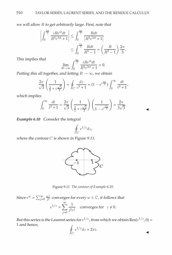
510 TAYLOR SERIES, LAURENT SERIES, AND THE RESIDUE CALCULUS
we will allow R to get arbitrarily large. First, note that&&&&&
Y 2!3
0
iReitdt
R3e3it + 1
&&&&& +Y 2!
3
0
Rdt&&R3e3it + 1&&
+
Y 2!3
0
Rdt
R3" 1
=
2R
R3" 1
32%
3.
This implies that
limR('
Y 2!3
0
iReitdt
R3e3it + 1= 0.
Putting this all together, and letting R 3 -, we obtain
2%,
3
C1
32 + i
$3
2
D
=
\
C
dz
z3 + 1= (1 " ei 2!
3 )
Y '
0
dt
t3 + 1,
which impliesY '
0
dt
t3 + 1=
2%,
3
C1
32 + i
$3
2
DC1
1 " ei 2!3
D
=2%
3,
3.
"
Example 6.10 Consider the integral\
Ce1/zdz,
where the contour C is shown in Figure 9.11.
C1!1
Figure 9.11 The contour of Example 6.10.
Since ew =;'
j=0wj
j! converges for every w # C, it follows that
e1/z ='+
j=0
1
j!zjconverges for z $= 0.
But this series is the Laurent series for e1/z , from which we obtain Res(e1/z, 0) =1 and hence, \
Ce1/zdz = 2%i.
"

THE RESIDUE CALCULUS 511
Example 6.11 Consider the integralZ'
0sin x
x dx. SinceY '
0
sin x
xdx = Im
2Y '
0
eix
xdx
3,
we will evaluate]C
eiz
z dz, where C = (C1, C2, C3, C4), as shown in Figure9.12.
C1
C2
C3
C4
R$!$!R
Figure 9.12 The contour of Example 6.11.
To evaluate each of these integrals, we note that:Y
C1
eiz
zdz = "
Y
C&($)
eiz
zdz,
Y
C2
eiz
zdz =
Y R
(
eit
tdt,
Y
C3
eiz
zdz =
Y $
0
eiReit
ReitiReitdt = i
Y $
0eiReit
dt, and
Y
C4
eiz
zdz =
Y "(
"R
eit
tdt.
Since]C
eiz
z dz = 0 (Why?), it follows that
0 = "
Y
C&($)
eiz
zdz + i
Y $
0eiReit
dt +
Y R
(
eit
tdt +
Y "(
"R
eit
tdt
= "
Y
C&($)
eiz
zdz + i
Y $
0eiReit
dt +
Y R
(
eit" e"it
tdt
= "
Y
C&($)
eiz
zdz + i
Y $
0eiReit
dt +
Y R
(
2i sin t
tdt.
From this we obtain
2i
Y '
0
sin t
tdt = lim
((0
(Y
C&($)
eiz
zdz
)" lim
R('i
Y $
0eiReit
dt. (9.34)

512 TAYLOR SERIES, LAURENT SERIES, AND THE RESIDUE CALCULUS
To evaluate the limits in the above, we note that&&&&
Y $
0eiReit
dt
&&&& =
&&&&
Y $
0eiR cos te"R sin tdt
&&&&
+
Y $
0e"R sin tdt,
the last of which 3 0 as R 3 - due to Jordan’s inequality (see Exercise 7.24on page 358 in Chapter 7). Also, by the fractional residue theorem,
lim((0
(Y
C&($)
eiz
zdz
)= i% Res
(eiz
z, 0
)= i%.
All of this allows us to rewrite (9.34) as
2i
Y '
0
sin t
tdt = i%,
which obtains Y '
0
sin t
tdt =
%
2.
"
7 SUPPLEMENTARY EXERCISES
1. Find the power series expansion and radius of convergence for f : C \ {&2} , C
given by f (z) = 12+z
in powers of z. How about in powers of z & i? In powers of z + 2?
2. Find the radius of convergence for each of the following:
a);%
j=0j
3
(j+3)4j zj
b);%
j=0j!xj
e2j c);%
j=1
, 2j+5j
j5
-z
jd)
;%j=1
(z!#)j
j5
e);%
j=12j (z+i)j
j(j+1) f );%
j=1(z+1)j
j2j g);%
j=15j (x!1)j
j2
3. Use the series expansion 11!z
=;%
j=0 zj to find the series expansion of 1
(1!z)2 =(;%
j=0 zj
)(;%j=0 z
j
). What is the radius of convergence?
4. Use the expansions f (z) = 11!z
=;%
j=0 zj and g(z) = 1
1!z2 =;%
j=0 z2j to find the
expansion for f (z)g(z) . Does this expansion reduce to 1 + z for appropriate values of z?
5. Consider the function f : R \ {0} , R given by f (x) = 1x
. Find the Taylor seriesexpansion for f in powers of x & 1. Where does it converge?
6. Find the Taylor series expansion for the function f : C \ {i} , C given by f (z) =e
z
z!iin powers of z + 1. Where does it converge?
7. Confirm that the product of the Taylor series representation for ex with that of e
iy
yields that of ez , as it must.

SUPPLEMENTARY EXERCISES 513
8. Differentiate the Taylor series expansion for sin z centered at z0 = 0 term-by-termto obtain the Taylor series for cos z centered at z0 = 0.
9. Find the Taylor series representation for f (z) = 1z
centered at z0 = &1. Differentiateit term-by-term to find the Taylor series for g(z) = 1
z2 .
10. Use multiplication and division of power series to find the power series represen-tations centered at the origin for the following:
a) ln(1+x)1+x
b) cos2x c) e
x sin x d) ez
1!z2 e) sin 2x = 2 sin x cos x
11. Let x
ex!1 =;%
j=0Bj
j! xj . The coefficients Bj for j ' 1 are called the Bernoulli
numbers. Show that B3 = B5 = B7 = · · · = 0, and calculate B1, B2, B4, and B6.
12. Find the Taylor series expanded around x0 = 0 for the following functions:
a) F (x) =Z
x
0sin t
tdt b) G(x) =
Zx
0
, sin t
t
-2dt.
13. Consider the function f : C\{±3} , C given by f (z) = 1z2!9 .
a) Find the Taylor series for f (z) that is valid for |z| < 3.
b) Find the Laurent series for f (z) that is valid for 0 < |z & 3| < 6 and Res(f (z), 3).
c) Find the Laurent series for f (z) that is valid for |z| > 6 and Res(f (z), 3).
14. Find the Laurent expansion for the function f : C\{±1} , C given by f (z) = 1z2+1
in powers of z & 1. Where does it converge? How about in powers of z + 1? Wheredoes it converge now?
15. Find the Laurent expansion for the function given by f (z) = cos z
z2+(1!i)z!ithat
converges for 0 < |z & i| <*
2. How about for |z & 1| <*
2?
16. Find the Laurent expansion for the function given by f (z) = 1z(z!1)(z!2) that
converges on A10(0). How about on A
21(0)? How about on A
%2 (0)?
17. Find the Laurent series for the following:
a) csc z on A#
0 (0) b) 1ez!1 on A
2#
0 (0) c) ez
z (z2+1) on A10(0).
18. Classify the indicated singularities:
a) f (z) = z2!2z+3z!2 at z0 = 2 b) f (z) = sin z
z4 at z0 = 0 c) f (z) = ez!1z
at z0 = 0.
19. Classify the singularities at z0 = 0 for the following:
a) f (z) = z sin 1z
b) f (z) = z cos 1z
c) f (z) = Log(z+1)z2 .
20. Show that a complex function f has a removable singularity at / if and only if f
is constant.
21. Show that a complex function f is entire with a pole at / of order m if and onlyif f is a polynomial of degree m.

514 TAYLOR SERIES, LAURENT SERIES, AND THE RESIDUE CALCULUS
22. Show thatZ 2#
0dt
2+cos t= 2#"
3. To do so, express cos t in terms of the complex expo-
nential function to show that the given integral expression is equivalent to 2i
]
C1(0)
dz
z2+4z+1 .
Then use residues to obtain the value 2#"3
. For a > b > 0, show more generally thatZ 2#
0dt
a+b cos t= 2#*
a2!b2.
23. Evaluate: a)]
C1(0)
ez
4z2+1 dz b)]
C2(0)
z3+1
(z+1)(z2+16) dz c)]
C2(0)
5z!2z (z!1) dz d)
]
C
dz
(z2!1)2+1
where C = [2, 2 + i, &2 + i, &2, 2].
24. Evaluate the following real integrals.
a)Z%
0dx
(1+x2)2 b)Z%
0x
2+3(1+x2)(4+x2) dx c)
Z 1!1
dx
(2!x2)*
1!x2d)
Z%0
x2+1
x4+5x2+4dx
e)Z%
0cos x
1+x2 dx f )Z%
0dx
(1+x)"
xg)
Z %0
cos x
1+x4 dx h)Z%
0ln x
x4+1dx i)
Z%0
ln x
x2+1 dx
j)Z%
0
, sin x
x
-2dx k)
Z%0
dx"x(x2+1)
l)Z%!%
dx
x2+4x+2m)
Z%0
x sin 2x
x4+1dx
n)Z%
0cos x!1
x2 dx o)Z%!%
dx
x2+x+1 p)Z%!%
ex/2
1+ex dx
25. What kind of singularity does the function f : C \ {0} , C given by f (z) =,ez & 1
-!1have at z0 = 0? Find three nonzero terms of the Laurent series expansion
of this function centered at z0 = 0. Then, find the largest value of R > 0 such that theLaurent series converges on 0 < |z| < R.
26. Show that the function f : C \ {0} , C given by f (z) = z
ez!1 has a removablesingularity at z0 = 0. Find the first two terms in the Laurent series expansion for f ,and find the radius of convergence.
27. For each of the following, find the residue and determine the type of singularity:
a) Res,ze
1/z , 0-
b) Res, 1!e
2z
z4 , 0-
c) Res,
e2z
(z!1)2 , 1-
d) Res,
z
cos z, #
2
-e) Res
,e
z
z2+#2 , i'-
f ) Res,
ez
z2+#2 , &i'-
28. Let the function f : C , C be entire such that limz&%
f (z) = /. Show that f must
be a polynomial.
29. True or false? Let f : C , C be an entire function.
a) If f (x) = 0 on (0, 1), then f (z) = 0 for all z " C.
b) If f (x) is bounded on R, then f (z) is constant on C.
30. Find the radius of convergence for;%
n=1 n2/n
zn and find a point on the circle of
convergence where the series diverges.
31. Fix !, " " C. Find the radius of convergence for;%
n=1
,!
n + "n-z
n.
10COMPLEX FUNCTIONS AS MAPPINGS
Mathematicians do not study objects, but relations between objects. Thus, they arefree to replace some objects by others so long as the relations remain unchanged.Content to them is irrelevant: they are interested in form only.
Jules Henri Poincaré
1 THE EXTENDED COMPLEX PLANE
In this section we will establish a convenient correspondence between thecomplex plane and the surface of a sphere known as the Riemann sphere. Aconsequence of this mapping will be a well-defined notion of the point at in-
finity in what is referred to as the extended complex plane [C / C % {-}.
Stereographic Projection and the Riemann Sphere
Consider the unit sphere S /
.(x1, x2, x3) # R3 : x2
1 + x22 + x2
3 = 1/' R3, and
let N = (0, 0, 1) be the “north pole“ of S. Consider the plane R2' R3 inter-
secting the sphere S along the equator as shown in Figure 10.1, and define amap f according to the following rule. For the ray emanating from N and in-tersecting the sphere S at (x1, x2, x3) and the plane at (x&1, x&2) define the mapf : S \ {N} 3 R2 by f (x1, x2, x3) = (x&1, x&2). To develop an algebraic formulafor f , we consider the line in R3 given by,
tx1, tx2, 1 + t(x3 " 1)-
for t # R.
This line contains the point N and the point with coordinates (x1, x2, x3) # S.To find the coordinates of the point in the plane that also lies on the line,set the third coordinate of the line to zero and obtain t = 1
1"x3. This yields
(x&1, x&2) =, x1
1"x3, x2
1"x3
-, and therefore f (x1, x2, x3) =
, x11"x3
, x21"x3
-. Clearly the
real plane can be replaced by the complex plane, and doing so lets us defineF : S \ {N} 3 C given by
F (x1, x2, x3) =x1
1 " x3+ i
x2
1 " x3. (10.1)
515

516 COMPLEX FUNCTIONS AS MAPPINGS
N
(x1, x2, x3)
(x"
1, x"
2)
Figure 10.1 Stereographic projection.
We will now show that F is a one-to-one correspondence. To see that Fis one-to-one, consider (x1, x2, x3) and (y1, y2, y3) both in R3 and such thatF (x1, x2, x3) = F (y1, y2, y3). This implies that x1+ix2
1"x3= y1+iy2
1"y3, which in turn
yieldsx2
1+x22
(1"x3)2 =y2
1+y22
(1"y3)2 . Since x21 + x2
2 + x23 = y2
1 + y22 + y2
3 = 1, this obtains
1"x23
(1"x3)2 =1"y2
3(1"y3)2 , which in turn yields that x3 = y3. (Why?) It is then easy to
see that x1 = y1 and x2 = y2, and therefore that F is one-to-one. To see thatF is onto, let w = & + i- # C be arbitrary. We will find (x1, x2, x3) # S \ {N}
such that F (x1, x2, x3) = & + i-. In fact, simple algebra obtains
x1 =2&
1 + &2 + -2, x2 =
2-
1 + &2 + -2, x3 =
&2 + -2" 1
1 + &2 + -2,
and so F is onto. Since F is one-to-one and onto, it has an inverse. We leaveit to the reader to show that F"1 : C 3 S \ {N} is given by
F"1(z) =
2z + z
|z|2 + 1,"i(z " z)
|z|2 + 1,|z|2 " 1
|z|2 + 1
3. (10.2)
! 10.1 Verify that F!1 is the inverse function to F .
We may extend the function F"1 and thereby extend the complex plane to in-clude an ideal point at infinity, denoted by -, in the following way. Note thatthere is no element of C that gets mapped by F"1 to N . In fact, we can showthat as (x1, x2, x3) approaches N , the magnitude of F (x1, x2, x3) becomes un-bounded. To see this, consider that
|F (x1, x2, x3)|2 =x2
1 + x22
(1 " x3)2=
1 " x23
(1 " x3)2=
1 + x3
1 " x3,
from which it follows that lim(x1,x2,x3)(N
|F (x1, x2, x3)|2 = -. Motivated by this,
we define the point at infinity, denoted by -, and adjoin it to the complex
plane C. We then define the extension [F"1 of F"1 to be the one-to-one corre-

THE EXTENDED COMPLEX PLANE 517
spondence [F"1 : C % {-} 3 S given by
[F"1(z) =
EF"1(z) if z # C
N if z = -
. (10.3)
Of course, we can similarly extend F to all of S by defining [F : S 3 C% {-}
according to
[F (x1, x2, x3) =
EF (x1, x2, x3) if (x1, x2, x3) # S \ {N}
- if (x1, x2, x3) = N. (10.4)
Then the functions [F"1 and [F are inverses of each other. This discussionmotivates the following definition.
Definition 1.1 The point at infinity, denoted by -, is defined as the unique
preimage of the point N # S under the mapping [F"1 : [C 3 S corresponding
to the stereographic projection described above. The set [C / C % {-} iscalled the extended complex plane.
Note that - is not a point in C. Yet it will be convenient to sometimes refer
to points in C '[C that are “near“ -. To do this properly, we must develop
a consistent notion of “distance“ from points in C '[C to -. This might
not appear possible since the distance from any point z0 # C '[C to -
would seemingly be infinite, no matter how large |z0| might be. The trick isto define a new distance function (called a metric) between any two points
in [C in terms of a well-defined distance between the corresponding points onthe sphere S. Then, with this new distance function, we can say that a point z0
in C '[C is “close“ to - exactly when the corresponding point 00 = [F"1(z0)
on the sphere is “close“ to N . One such distance function defined on thesphere is just the Pythagorean distance in R3. Define the distance function
d : [C .[C 3 R for any z, z& # [C by
d(z, z&) /&& [F"1(z) " [F"1(z&)
&&.
Then it can be shown that
d(z, z&) =
RT
U
2|z"z!|,
(1+|z|2)(1+|z!|2)for z, z& in C
2,
1+|z|2for z in C and z& = -
,
and that d(z1, z2) ! 0 with equality if and only if z1 = z2, d(z1, z2) = d(z2, z1),
and d(z1, z2) + d(z1, z3) + d(z2, z3) for all z1, z2, and z3 in [C. These proper-ties are the necessary ones of any well-defined metric or distance function inEuclidean space.
! 10.2 Verify the claims made above about the distance function d.

518 COMPLEX FUNCTIONS AS MAPPINGS
! 10.3 Using the new distance function on [C described above, show that for any
given $ satisfying 0 < $ < 2, any z " [C will be within $ of / if |z| >
*4$2 & 1. What
if $ ' 2?
Continuity of the Stereographic Projection
We may now establish that the stereographic projection mapping [F"1 is con-tinuous on C. Continuity is a “metric dependent“ property, and so we needto check it under each of the metrics we now have on C. To see continuity
in the old metric, note that [F"1 = F"1 on C, and simply consider (10.2). To
establish continuity for the d metric, fix z& # [C and let ! > 0 be given. We
must find . > 0 such that d(z, z&) < . implies |[F"1(z) " [F"1(z&)| < !. But
d(z, z&) / |[F"1(z) " [F"1(z&)|, and so taking . = ! does the trick. In fact, the d
metric can measure distances to - as well, and therefore continuity of [F"1
also holds at -. Because of this, we may hereafter think of S as a represen-
tation of [C and we will refer to S as the Riemann sphere. Through this specialidentification we can relate convergence in the complex plane to convergenceon S and vice versa. In fact, convergence in C as previously defined (with theusual distance function) is preserved under the new distance function d. Thatis, lim zn = z0 in the usual metric if and only if lim d(zn, z0) = 0. To see this,
note that lim zn = z0 if and only if lim [F"1(zn) = [F"1(z0) by continuity of[F"1. This in turn holds if and only if lim |
[F"1(zn) " [F"1(z0)| = 0, which istrue if and only if lim d(zn, z0) = 0. Also, using d we can extend the idea of
convergence in C to include sequences {zj} ' C '[C that converge to - in
the following way. Let {zj} be a sequence with zj # C '[C for j ! 1. Then,
denoting the traditional symbol of unboundedness by +- (rather than -,which now has a different meaning in this chapter), we have
limj(+'
d(zj ,-) = limj(+'
2*1 + |zj |
2= 0 if and only if lim
j(+'|zj | = +-.
We have established the following result.
Proposition 1.2 Let {zj} be a sequence with zj # C '[C for j ! 1. Then
limj(+'
zj = - if and only if limj(+'
|zj | = +-.
The point at infinity is said to “compactify“ the complex plane, since with
it and the new metric d the set [C = C % {-} is the image of the compact
set S under the continuous mapping [F . As we will see, the point at infinitycan be a convenience when discussing unbounded sets in the complex planeand mappings of them. For example, we will adopt the following rather typ-
ical convention: Let A be any subset of C. Since C '[C, the set A may also
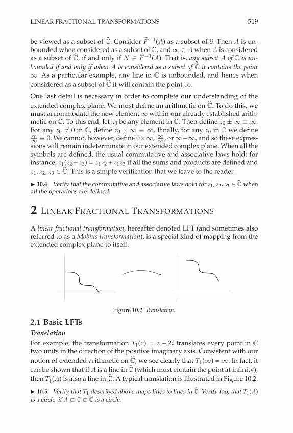
LINEAR FRACTIONAL TRANSFORMATIONS 519
be viewed as a subset of [C. Consider [F"1(A) as a subset of S. Then A is un-bounded when considered as a subset of C, and - # A when A is consideredas a subset of [C, if and only if N #
[F"1(A). That is, any subset A of C is un-
bounded if and only if when A is considered as a subset of [C it contains the point-. As a particular example, any line in C is unbounded, and hence when
considered as a subset of [C it will contain the point -.
One last detail is necessary in order to complete our understanding of the
extended complex plane. We must define an arithmetic on [C. To do this, wemust accommodate the new element - within our already established arith-metic on C. To this end, let z0 be any element in C. Then define z0 ±- / -.For any z0 $= 0 in C, define z0 . - / -. Finally, for any z0 in C we definez0' / 0. We cannot, however, define 0.-, '
' , or -"-, and so these expres-sions will remain indeterminate in our extended complex plane. When all thesymbols are defined, the usual commutative and associative laws hold: forinstance, z1(z2 + z3) = z1z2 + z1z3 if all the sums and products are defined and
z1, z2, z3 #[C. This is a simple verification that we leave to the reader.
! 10.4 Verify that the commutative and associative laws hold for z1, z2, z3 " [C whenall the operations are defined.
2 LINEAR FRACTIONAL TRANSFORMATIONS
A linear fractional transformation, hereafter denoted LFT (and sometimes alsoreferred to as a Mobius transformation), is a special kind of mapping from theextended complex plane to itself.
Figure 10.2 Translation.
2.1 Basic LFTsTranslation
For example, the transformation T1(z) = z + 2i translates every point in C
two units in the direction of the positive imaginary axis. Consistent with our
notion of extended arithmetic on [C, we see clearly that T1(-) = -. In fact, it
can be shown that if A is a line in [C (which must contain the point at infinity),
then T1(A) is also a line in [C. A typical translation is illustrated in Figure 10.2.
! 10.5 Verify that T1 described above maps lines to lines in [C. Verify too, that T1(A)
is a circle, if A ! C ! [C is a circle.

520 COMPLEX FUNCTIONS AS MAPPINGS
Rotation and Scaling (Dilation)
Fix nonzero z0 # C, and let T2 : [C 3[C be given by
T2(z) = z0z.
Clearly T (0) = 0 and T (-) = -. For any other z # C '[C we may employ
polar form with z0 = r0ei"0 and z = rei" to obtain
T2(z) = r0rei("+"0).
From this we see that the point z = rei" gets mapped to a new point whoseradius is rescaled by r0 and whose argument is increased by $0. Therefore amapping of the form T2(z) = z0z has the effect of rotating by $0 and scalingby a factor of r0. In the case where the angle $0 is negative, the rotation isclockwise of magnitude |$0|, whereas if $0 is positive the rotation is counter-clockwise. If r0 is greater than 1 the scaling effect is a stretching, whereas if r0
is less than 1 the scaling effect is a shrinking. As an explicit example, considerT2(z) = iz. Then
T2(z) = iz = ei$/2rei" = rei("+!2 ),
and it is easy to see that in this case T2 rotates points counterclockwise throughan angle of $
2 radians (see Figure 10.3). Again, consistent with our notion of
Figure 10.3 Rotation by 90 degrees.
extended arithmetic on [C, we see clearly that T2(-) = -. As in the case oftranslations, it can be shown that T2 takes lines to lines, and circles to circles.
! 10.6 Show that if A ! [C is a line, and if B ! C ! [C is a circle, then T2(A) is a lineand T2(B) is a circle.
Inversion
Let T3 : [C 3[C be given by
T3(z) =1
z.
Clearly, T (0) = - and T (-) = 0. To determine the image of any other point
in C '[C, note that in polar coordinates we have
T3(z) =1
z=
1
rei"=
1
re"i".

LINEAR FRACTIONAL TRANSFORMATIONS 521
From this we see that T3 rescales z by a factor of 1r2 , and rotates z through an
angle "2$. This rotation amounts to a reflection across the real axis.
!
!
r
r!1
Figure 10.4 Inversion.
Owing to the rescaling,1 any point inside the unit circle will be mapped byT3 to the exterior of the unit circle, and vice versa (see Figure 10.4). Points onthe unit circle will be mapped back to the unit circle.
! 10.7 Let A ! [C be a line that passes through the origin. Show that T3(A) is also aline. Explain why the image of a line that does not pass through the origin cannot bea line. In fact, show that such a line is mapped to a circle.
! 10.8 Find the image of the square A = [0, 1, i, 0] ! C ! [C under T3.
! 10.9 Let B ! C ! [C be a circle. Show that T3(B) is a circle if B does not passthrough the origin, but is a line if B does pass through the origin.
2.2 General LFTs
We now note the following important results regarding LFTs.
Proposition 2.1 Let T : [C 3[C be an LFT given by T (z) = az+b
cz+d . Then,
a) The mapping T is continuous on [C and is differentiable on
C \ {"dc} if c $= 0, and on C if c = 0.
b) The mapping T is a one-to-one correspondence from [C to itself.
c) The mapping T has an inverse T"1, which is also an LFT.
! 10.10 Prove the above. Begin by computing the derivative of T (z).
We will now show that the special-case LFTs T1, T2, and T3 from the last sub-section are the building blocks of every LFT.
1If one were to also consider more general inversions that mapped points on a circle ofradius R to itself, rather than just the inversions that map points of the unit circle to itself as wedo here, it would in fact be advisable to characterize the scaling differently. For a discussion ofthis more general inversion see [Nee99].

522 COMPLEX FUNCTIONS AS MAPPINGS
Proposition 2.2 Every LFT can be written as a composition of mappings of thetype T1, T2, and T3.
PROOF There are two cases.
Case 1: c = 0. In this case, d $= 0 and a $= 0, and we have
T (z) =a
dz +
b
d=,T1 ; T2
-(z),
where T1(z) = z + bd and T2(z) = a
dz.
Case 2: c $= 0. In this case,
T (z) =a
c"
(ad " bc
c
) 1
cz + d.
From this we may write
T (z) =, [T1 ; T2 ; T3 ; T1 ;
[T2-(z),
where [T2(z) = cz, T1(z) = z + d, T3(z) = 1z , T2(z) = "
,ad"bc
c
-z, and [T1(z) =
ac + z. #
It can be shown that LFTs map lines to lines or circles, and circles to lines orcircles. We leave this to the reader.
! 10.11 Suppose T is an LFT. If A ! [C is a line, show that T (A) is a line or a circle.
When will it be a circle? If B ! C ! [C is a circle, show that T (B) is a line or a circle.When will it be a line?
The simple proof of the following result is left to the reader.
Proposition 2.3 If S and T are both LFTs, then S ; T is also an LFT.
! 10.12 Prove the above.
Example 2.4 We will specify an LFT that maps the points "1, 0, and 1 to thepoints "i, 1, and i, respectively. To do so, let T (z) = az+b
cz+d . We will determinea, b, c, and d satisfying the above. Note that since T (0) = 1, we must haveb = d. Also, T (±1) = ±i, which implies a+b
c+b = i and "a+b"c+b = "i. Solving these
two equations for a and c in terms of b obtains a = ib and c = "ib. Overall wehave
T (z) =ibz + b
"ibz + b=
iz + 1
"iz + 1.
"
! 10.13 Find an LFT that maps 0, 1, and / to 1, 0, 2i, respectively.

LINEAR FRACTIONAL TRANSFORMATIONS 523
The above example illustrates that one can specify an LFT by specifying itsaction on three distinct points. This might be surprising, since the formulafor an LFT involves four complex numbers a, b, c, and d. In fact, we will show
that specifying the images of three distinct points z1, z2, and z3 in [C is suf-ficient to characterize an LFT completely. One way to see this [Nee99] is tofirst consider what are called the fixed points of an LFT. The point z0 is a fixedpoint of the LFT given by T (z) = az+b
cz+d if T (z0) = z0. Simple algebra revealsthat an LFT that is not the identity mapping can have at most two such fixed points,since the equality T (z0) = z0 amounts to a quadratic polynomial in z0.
! 10.14 Show that if c %= 0 then the fixed points of T lie in C. Show too that if c = 0then / is a fixed point, and if a = d as well, so that T (z) = z + b, then / is the onlyfixed point.
Given the above, if T is an LFT taking the distinct points z1, z2, z3 in [C to thepoints w1, w2, w3, then it is unique. To see this, suppose S is another LFT thatalso maps z1, z2, and z3 to w1, w2, and w3. Then S"1 is an LFT, and S"1
; Tis an LFT that takes each of z1, z2, and z3 to itself. This implies that S"1
; Tis the identity mapping, and hence S = T . Finally, note too that for any three
distinct points z1, z2, and z3 in [C and three distinct image points w1, w2, and
w3 in [C we can always find an LFT that maps each zi to each respective wi
for i = 1, 2, 3. This is left to the reader in the following exercise.
! 10.15 Show that the equation (w!w1)(w2!w3)(w!w3)(w2!w1) = (z!z1)(z2!z3)
(z!z3)(z2!z1) implicitly defines an
LFT given by w = T (z) that maps z1, z2, and z3 to w1, w2, and w3, respectively. Theexpression on each side of the equality implicitly defining w in terms of z is called across ratio.
! 10.16 Use the above discussion to revisit Example 2.4.
! 10.17 Consider the distinct points z1, z2, and z3 in C as shown in Figure 10.5. Find
z1
z2z3
Figure 10.5 The situation in Exercise 10.17
an LFT that takes z1, z2, and z3 to w1, w2, and /, respectively, with w1 < w2 real. If T
is the LFT so found, show that Im,T (z)
-= 0 if and only if z " C where C is the circle
containing z1, z2, and z3. If z0 is any point inside the circle C show that T (z0) is inthe upper half-plane. Likewise, show that points outside the circle C get mapped tothe lower half-plane. Can you show that Int(C) is mapped onto the upper half-plane?Can you use this to find a map from the upper half-plane to the unit disk?

524 COMPLEX FUNCTIONS AS MAPPINGS
Mapping the Right Half-Plane to the Unit Disk
We now show that we can map, via LFT, the right half-plane to the unit diskwith the imaginary axis mapped to the unit circle. To this end, consider theLFT given by T (z) = az+b
cz+d , and suppose we wish to map the points "i, 0, ito the points i, 1,"i, respectively. Since f (0) = 1, we have d = b, and sincef (±i) = >i we have
ai + b
ci + d= "i and
"ai + b
"ci + d= i.
Solving for a, b, c, and d, we obtain c = b and d = "a. Therefore we may takeas our mapping
f (z) =1 " z
1 + z.
Note that multiplying a, b, c, d by a constant does not change the linear trans-formation. (This is a clue, in fact, as to why only three distinct points needbe specified in order to characterize the LFT.) One can check that this LFTmaps the imaginary axis to the unit circle. To see that the right half-plane ismapped to the interior of the unit disk, note that 1 is in the right half-plane.If z is in the right half-plane too, then ("z) is in the left half-plane. Remem-bering that absolute values measure distance in the traditional way, we note
that |1 " z| < |1 + z| = |1 " ("z)|, and therefore |f (z)| = |1"z||1+z| < 1. We leave it
to the reader to show that the mapping is onto.
! 10.18 Show that the mapping constructed above is onto the open unit disk. Also,show that the imaginary axis is mapped onto the unit circle.
! 10.19 Find an LFT that maps the upper half-plane to the unit disk. Do this by firstmapping the upper half-plane to the right half-plane and then map the result to theunit disk via the LFT given above. You must apply Proposition 2.3.
! 10.20 Can you use Exercise 10.15 on page 523 to find a map from the right half-plane to the unit disk with the imaginary axis mapped to the unit circle?
3 CONFORMAL MAPPINGS
LFTs are a special subclass of important mappings that have the property thatthey “preserve angles.“ Such mappings are called conformal mappings, and thefollowing motivation for our formal definition of this class of mappings willmake this angle-preservation property more precise. For convenience in this
section, we restrict our attention to C (not [C).
3.1 Motivation and Definition
Consider a complex function f : D 3 C that is differentiable on D, and let z0
be in D. We wish to investigate conditions under which the function f , whenacting as a mapping, will preserve angles having their vertex at z0. To makethis idea more precise, consider any two smooth curves in D parametrized

CONFORMAL MAPPINGS 525
z1(t)
z2(t)
z"
2(t)
z"
1(t)
z0 w0
+"
1(t)+"
2(t)
+2(t)+1(t)
z!plane w!plane
((
Figure 10.6 Conformality.
by zi : [a, b] 3 C for i = 1, 2, such that for both i = 1, 2,
(i) zi(t0) = z0 for a < t0 < b,
(ii) z&i(t) is continuous and nonzero for a + t + b.
Geometrically, z&i(t0) can be thought of as a tangent vector to the curve pa-rameterized by zi(t) at the point zi(t0). Denote the angle between z&1(t0) andz&2(t0) by ', where ' # [0, 2%). Then if $i(t) is a continuous argument of z&i(t)note that ' = $2(t0)"$1(t0). We wish to see how ' transforms under the map-ping f . (It is useful to think of f as taking points z = x + iy # D from the“z-plane“ to points w = u + iv in the “w-plane“ as shown in Figure 10.6.) Tothis end, let 2i(t) = f
,zi(t)
-be the image of the curve zi(t) under the mapping
f . The chain rule yields2&i(t) = f &,zi(t)
-z&i(t), (10.5)
which has a continuous argument !i(t) if f &(z) $= 0 on D. It follows that
!2(t0) " !1(t0) =
9arg
(f &,z2(t0)
-)+ arg
(z&2(t0)
):
"
9arg
(f &,z1(t0)
-)+ arg
(z&1(t0)
):
= $2(t0) " $1(t0) = ',
and so the angle between the curves at z0 has been preserved. Also note thatif we think of z&i(t0) as the tangent vector to the curve zi(t) at z0, and 2&i(t0)as the tangent vector of the image curve at w0 = f (z0), then the differentiablemapping f has the effect according to equation (10.5) of acting on the tangentvector z&i(t0) by multiplying it by f &,zi(t0)
-= f &(z0) $= 0. Recall that f &(z0)
is just a complex number, and as such can be represented in polar form by
|f &(z0)|ei arg(f !(z0)). Seen this way, the mapping f then has the effect of stretch-ing or shrinking the tangent vector z&i(t0) by the factor |f &(z0)| and rotatingit by arg(f &(z0)). The key point here is to note that the smooth curve zi(t)passing through z0 was arbitrary, and for any choice of such a smooth curve,the mapping f has the same local effect on the tangent vector to the curve

526 COMPLEX FUNCTIONS AS MAPPINGS
at the point z0, namely, a stretching or shrinking by the same constant factor|f &(z0)| and a rotation by the same constant angle arg(f &(z0)). We refer to thisproperty of the scaling factor of f by saying that it scales uniformly in all direc-tions at z0. This and the uniformity of action by f on the angles subtended byvectors at z0 are what make it special, and we call such maps conformal. Thismotivates the following definition.2
Definition 3.1 Let f : D 3 C be differentiable on D and suppose z0 # D.If f &(z0) $= 0 then we say that f is conformal at z0. If f is conformal at eachpoint of D we say that f is conformal on D.
We give some examples.
Example 3.2 Consider the mapping f : C \ {1} 3 C given by f (z) = 1z"1 .
This map is conformal on its domain since f &(z) exists and is nonzero there.If w = f (z) = u + iv, then we may solve for x and y in terms of u and v toobtain
x =u2 + v2 + u
u2 + v2, y = "
v
u2 + v2.
The circle x2 + y2 = 1 and the line y = x in the z-plane are orthogonal at theirpoint of intersection z0 =
,1$2
, 1$2
-. The image in the w-plane of the line y = x
z0
w0
w-planez-plane
Figure 10.7 The situation in Example 3.2.
is the circle,u + 1
2
-2 +,v + 1
2
-2 = 12 , and the image of the circle x2 + y2 = 1
(minus the point (x, y) = (1, 0)) is the line u = "12 . The point corresponding to
z = 1 clearly gets mapped to the point at infinity. The image of the point ofintersection is w0 =
,"
12 ," 1
2$
2"2
-, and it can be seen in Figure 10.7 that the
image curves are also orthogonal at w0. "
2Some authors define a complex mapping f : D ( C to be conformal at a point z0 # Dif the mapping preserves angles at the point. This alone need not imply uniform scaling nearthe point. However, upon consideration of open connected sets mapped by f , the geometricproperty of angle preservation can be shown to obtain precisely when f is differentiable with f !
nonzero on the set. The uniform scaling property then comes along in the bargain; see [Nee99].

CONFORMAL MAPPINGS 527
Example 3.3 Let f : C 3 C be given by f (z) = ez . Then f is conformalon C since f &(z) = ez
$= 0 there. Consider the lines y = 0 and x = 0 in thecomplex plane. These lines are orthogonal at their point of intersection z0 = 0.The reader can easily verify that the image of the line x = 0 under f is thecircle u2 + v2 = 1 and the image of the line y = 0 is the ray from the originalong the positive real axis. The image of the point of intersection z0 = 0is w0 = f (z0) = 1. It is not hard to verify that the tangent to the circle isorthogonal to the ray at the point w0. "
! 10.21 Show that any LFT is conformal on C if c = 0, or on C \ {!d
c} if c %= 0.
It is convenient that conformality is preserved under compositions.
Proposition 3.4 Suppose f : Df 3 C is conformal at z0 # Df and that g :Dg 3 C is conformal at f (z0), where Dg 9 Rf . Then g ; f : Df 3 C is conformalat z0 # Df .
! 10.22 Prove the above proposition.
Points at which conformality of a mapping fail are called critical points of themapping. For example, the function f : C 3 C given by f (z) = zn for n ! 2has a critical point at z = 0. In fact, angles are multiplied by a factor of n there.To see this, consider a point z( = !ei" on the circle of radius ! < 1 centered atz = 0. Then w = f (z() = !nein" so that the vector corresponding to the point z(
has been “shrunk“ by a factor of !n"1 and rotated by an angle (n " 1)$. Thatis, the image point’s argument is n times the preimage point’s argument. Acircle that is parametrized to go around z = 0 once in the z-plane will haveits image go around f (0) = 0 in the w-plane n times. This means that eachpoint on the w-circle has n preimages on the z-circle. Near the critical pointz = 0 then, the function is not one-to-one. Also note that near the point z = 0the mapping f (z) = zn for n ! 2 has the effect of contracting, since a diskcentered at 0 and of radius ! < 1 is mapped to a disk centered at 0 of radius!n < ! < 1.
3.2 More Examples of Conformal Mappings
In this section we explore some other mappings of the complex plane to itself.
Example 3.5 Fix ' such that 0 < ' + %, and consider the open sector givenby A = {z # C : z = rei" with r > 0 and 0 < $ < '}. Let the mappingf : C \ ("-, 0] 3 C be given by f (z) = z$/&. We will find the image f (A) inthe w-plane (see Figure 10.8). Note that we may write
f (z) = z$/& = e!'Logz = e
!' (ln r+i") = e
!' ln rei!(' = r
!' ei!(' .
From this we see that the ray z = rei" for fixed 0 < $ < ' gets mapped

528 COMPLEX FUNCTIONS AS MAPPINGS
w"planez"plane
(
Figure 10.8 The region A in Example 3.5.
into the ray w = r!' ei!(' , which emanates from the origin of the w-plane and
makes an angle $"& as measured from the positive u-axis. It is now easy to
see that the sector A gets mapped into the upper half-plane. The boundaryray $ = 0 stays fixed while the other boundary ray $ = ' gets mapped to thenegative u-axis. "
! 10.23 Show that the mapping f is conformal. Also show that it maps its domainonto the upper half-plane.
! 10.24 Fix ! as before so that 0 < ! # '. Also, fix %0 " R. Consider the sectorA = {z " C : z = re
i% with r > 0 and %0 < % < %0 + !}. Using composition ofmappings, find a map from the sector A onto the upper half-plane. Now for any fixedz0 " C, do the same for the sector given by Az0 = {z " C : z = z0 + re
i% with r >
0 and %0 < % < %0 + !}. Can you find a map of Az0 to the unit disk?
Example 3.6 Consider f : C 3 C given by f (z) = ez, and suppose A = {z #
C : Im(z) = y0}, a horizontal line in the z-plane. Then for z # A, we havethat w = f (z) = exeiy0 . As x varies from "- to +- with y0 fixed, we see(as illustrated in Figure 10.9) that 0 < ex < +-, and hence the points onthe line in the z-plane are mapped to the points on a ray emanating from theorigin at angle y0 in the w-plane. If instead we consider the horizontal strip
z!plane w!plane
Figure 10.9 The region A in the latter part of Example 3.6.
B = {z # C : y1 + Im(z) + y2} where y2 " y1 + 2%, we see that B is mappedinto the sector {w # C : w = +ei# with + > 0 and y1 + & + y2}. "
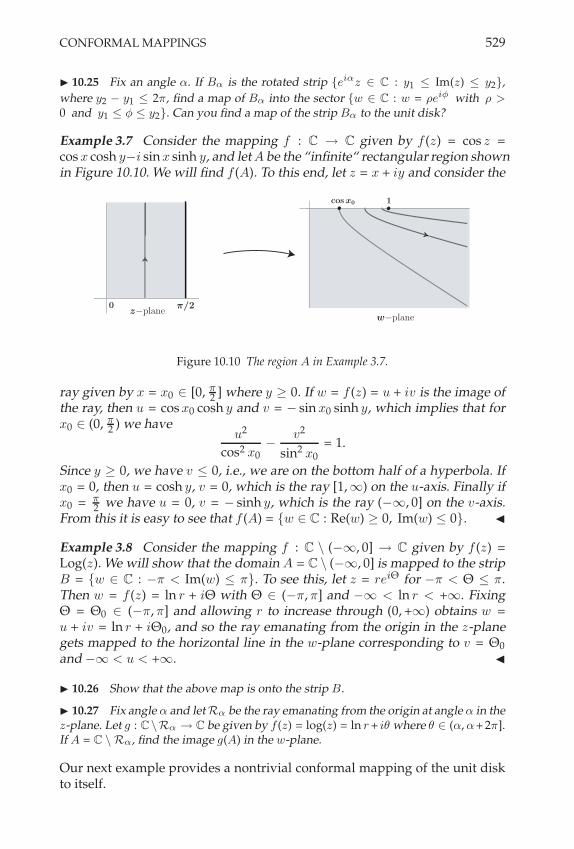
CONFORMAL MAPPINGS 529
! 10.25 Fix an angle !. If B! is the rotated strip {ei!z " C : y1 # Im(z) # y2},
where y2 & y1 # 2', find a map of B! into the sector {w " C : w = ,ei' with , >
0 and y1 # & # y2}. Can you find a map of the strip B! to the unit disk?
Example 3.7 Consider the mapping f : C 3 C given by f (z) = cos z =cos x cosh y"i sin x sinh y, and let A be the “infinite“ rectangular region shownin Figure 10.10. We will find f (A). To this end, let z = x + iy and consider the
0
cosx0 1
*/2
z!planew!plane
Figure 10.10 The region A in Example 3.7.
ray given by x = x0 # [0, $2 ] where y ! 0. If w = f (z) = u + iv is the image of
the ray, then u = cos x0 cosh y and v = " sin x0 sinh y, which implies that forx0 # (0, $
2 ) we haveu2
cos2 x0"
v2
sin2 x0= 1.
Since y ! 0, we have v + 0, i.e., we are on the bottom half of a hyperbola. Ifx0 = 0, then u = cosh y, v = 0, which is the ray [1,-) on the u-axis. Finally ifx0 = $
2 we have u = 0, v = " sinh y, which is the ray ("-, 0] on the v-axis.From this it is easy to see that f (A) = {w # C : Re(w) ! 0, Im(w) + 0}. "
Example 3.8 Consider the mapping f : C \ ("-, 0] 3 C given by f (z) =Log(z). We will show that the domain A = C \ ("-, 0] is mapped to the stripB = {w # C : "% < Im(w) + %}. To see this, let z = rei! for "% < ! + %.Then w = f (z) = ln r + i! with ! # ("%, %] and "- < ln r < +-. Fixing! = !0 # ("%, %] and allowing r to increase through (0, +-) obtains w =u + iv = ln r + i!0, and so the ray emanating from the origin in the z-planegets mapped to the horizontal line in the w-plane corresponding to v = !0
and "- < u < +-. "
! 10.26 Show that the above map is onto the strip B.
! 10.27 Fix angle ! and let R! be the ray emanating from the origin at angle ! in thez-plane. Let g : C\R! , C be given by f (z) = log(z) = ln r + i% where % " (!, !+ 2'].If A = C \ R!, find the image g(A) in the w-plane.
Our next example provides a nontrivial conformal mapping of the unit diskto itself.

530 COMPLEX FUNCTIONS AS MAPPINGS
Example 3.9 We define the unit disk to be U / N1(0). For z0 # U , define
Tz0 (z) /z " z0
1 " z0z.
Then Tz0 is differentiable on U (since |z0| < 1). We leave it to the reader toverify that Tz0 is conformal on U . We will now show that Tz0 maps the unitcircle to itself. To see this, let z0 = r0e
i"0 with r0 < 1, and suppose z = ei"#
*U . Then
&&&Tz0(ei")&&& =
&&&ei"" r0e
i"0
&&&&&1 " r0e"i"0ei"
&& =&&&ei"
&&&
&&&1 " r0ei("0"")
&&&&&1 " r0e"i("0"")
&& .
Since the numerator and the denominator in the last expression are conju-gates, it follows that |Tz0 (z)| = 1. By the maximum modulus theorem, itthen follows that U is mapped into itself since Tz0 is nonconstant. ThereforeTz0(z) # U for z # U , and so Tz0 is a nontrivial conformal mapping of U toitself. The reader can verify that the inverse transformation is given by
T"1(z) = T"z0 =z + z0
1 + z0z,
and note that the inverse is of the same form with z0 replaced by "z0. There-fore, T"z0 is a conformal mapping of U into itself too. Now, Tz0 and T"z0
being inverses, we have:
U = Tz0
,T"z0 (U )
-' Tz0(U ) ' U
This shows that Tz0 (U ) = U . The reader can verify that the mapping Tz0 isone-to-one, and therefore it is a one-to-one correspondence of the unit diskwith itself. "
! 10.28 Show that Tz0 is conformal on U . Also, verify that T!z0 is the inverse map-ping for Tz0 , and that Tz0 is one-to-one.
! 10.29 Suppose a " R, and consider T . eia
Tz0 . Show that T is also a conformalone-to-one correspondence of U with itself.
3.3 The Schwarz Lemma and the Riemann Mapping Theorem
We begin with a technical definition.
Definition 3.10 An open set D ' C is called simply connected if for everyclosed contour C ' D and w /# D,
nC (w) = 0.
Intuitively, a simply connected subset of C (or of R2) is one that contains no“holes.“ This is also sometimes described as a set within which any closed

CONFORMAL MAPPINGS 531
Figure 10.11 Examples of a simply connected region (left) and a region that is not simplyconnected (right).
contour can be “shrunk down“ to a point without ever leaving the set (seeFigure 10.11).
Example 3.11 The interior of a simple closed contour C& is a simply con-nected open set. In fact, if C ' Int(C&), then nC (w) is constant on the con-nected set Ext(C&) = C&
% Ext(C&) by Theorem 2.7 of Chapter 8. Since that setis unbounded, nC (w) is zero there. "
! 10.30 Let D ! C be a simply connected open set. If f : D , C is differentiableand C ! D is a closed contour, show that
]C
f (z)dz = 0.
! 10.31 Show that a star-shaped region is simply connected.
The Schwarz Lemma
The following is a significant result in the theory of complex functions asmappings. Its proof is a consequence of the maximum modulus theorem.
Theorem 3.12 (The Schwarz Lemma)Let U = {z # C : |z| < 1} be the unit disk. Suppose f : U 3 C is differentiable andsatisfies f (0) = 0 and f (U ) ' U , i.e., |f (z)| + 1 for z # U . Then
|f (z)| + |z| for all z # U .
If equality holds at some z $= 0, then f (z) = eiaz for some a # R.
Note that the final condition and its particular conclusion imply that if |f (z)| =|z| for some nonzero z in U , then the map f amounts to a rigid rotation.
PROOF Note that, since f (0) = 0, the function g(z) /f (z)z is differentiable
on the unit disk if it is defined to be f &(0) at z = 0. Fix r < 1. On the circleCr = {z : |z| = r},
|g(z)| =
&&&&f (z)
z
&&&& +1
r(10.6)
by the assumption on f . By the maximum modulus theorem, the inequalityholds for all z satisfying |z| + r. Take the limit as r 3 1" and we find that|g(z)| + 1 for all z, with equality implying g is constant. (See also the exercise

532 COMPLEX FUNCTIONS AS MAPPINGS
below.) This means that |f (z)| + z for all z # U , and the final assertion followsas well. #
! 10.32 Use the maximum modulus theorem to finish the proof of the above lemma.Prove also that
&&f #(0)&& # 1.
A consequence of the Schwarz lemma is that any conformal one-to-one map-ping of U to itself must be of a particular form.
Proposition 3.13 If f : U 3 U is a conformal one-to-one correspondence of Uwith itself, then there exists z0 # U , a # R, so that
f (z) = eiaTz0 (z) = eia z " z0
1 " z0z.
PROOF Take z0 to be the unique root of f and consider g : U 3 U given byg(z) = (f ; T"z0 )(z). Then g(0) = 0, since T"z0 (0) = z0, so that the Schwarzlemma applies. Therefore |g(z)| + |z|. Now g is also a one-to-one correspon-dence of the disk with itself, since T"z0 and f are. We may consider its in-verse h : U 3 U given by h(z) = g"1(z). Then h(0) = 0 too, and we apply theSchwarz lemma to h. We have that |h(z)| + |z| for all z # U . Therefore,
|z| = |h(g(z))| + |g(z)| + |z| ,
which means that |g(z)| = |z| for all z # U . Thus g is a rotation, g(z) = eiaz forsome a # R. Since g = f ; T"z0 , it then follows that f = g ; T"1
"z0= g ; Tz0 .
Thus f (z) = eiaTz0 (z). #
! 10.33 Suppose f1, f2 : D , U are differentiable and are conformal one-to-one
correspondences. Show by considering the composite mapping f23f!11 and applying
the above proposition, that for some a " R, z0 " U , f2 is given by f2(z) = eia f1(z)!z0
1!z0f1(z) .
The Riemann Mapping Theorem
The Riemann mapping theorem is a celebrated result in complex analysis.Originally stated and proved in Riemann’s doctoral thesis, the proof he pro-vided was dependent upon a result he called Dirichlet’s principle that waslater found to not necessarily apply to all the types of sets Riemann consid-ered.3 Subsequent refinements by a series of mathematicians (Weierstrass,Hilbert, Osgood, Carathéodory) firmly established the result. The proof israther technical and involves certain concepts and techniques we have notdeveloped, and we therefore omit it.4 Yet, it provides a nice culmination tothe present chapter, and an enticement to further reading.
3In particular, the nature of the boundary of the set is critical. In fact, the behaviors of func-tions and solutions to equations at and near the boundaries of the domains on which they areapplied are often complicated and/or difficult to establish.
4See [Ahl79].

CONFORMAL MAPPINGS 533
Theorem 3.14 (The Riemann Mapping Theorem)Let D ' C be an open, connected, and simply connected proper subset of the complexplane. Then there exists a differentiable function f : D 3 C such that f &(z) $= 0 onD, and so that f establishes a conformal one-to-one correspondence between D andU = N1(0).
! 10.34 In the statement of the above theorem, why can’t the set D be the wholecomplex plane? What would that imply?
! 10.35 Suppose D1, D2 ! C are open, connected, and simply connected. Use theRiemann mapping theorem to show that there exists a conformal one-to-one corre-spondence f : D1 , D2.
Note that the result is relatively simple to state, and is schematically illus-trated in Figure 10.12. Its consequences are significant, in that if one is work-ing on a problem in a complicated domain D ' C, even with a somewhatcomplicated boundary, one can map the problem to the much nicer environ-ment that is the unit disk. However, while the existence of such a mappingis guaranteed by the theorem, much as with the Tietze extension theorem ofChapter 4, there is no algorithm suggested for finding the map that does thejob. Even the proof of the theorem does not provide a practical means for ob-taining the desired map, much in the same way the Tietze extension theoremfailed to provide such details. It is also worth pointing out that there is noanalogous result for mappings from higher-dimensional Euclidean spaces tothemselves. Because of the Riemann mapping theorem, it is sometimes jokedthat those who study and understand the analysis of differentiable complexfunctions on the unit disk U know all there is to know about the subject. Butwe suggest you consult the bibliography to learn even more.
z!plane w!plane
Figure 10.12 The Riemann Mapping Theorem.

534 COMPLEX FUNCTIONS AS MAPPINGS
4 SUPPLEMENTARY EXERCISES
1. Find an LFT that maps 1, 0, &1 to i, /, 1, respectively.
2. Find an LFT that maps /, i, 0 to 0, i, /, respectively.
3. A fixed point of a function f is an element z such that f (z) = z.
a) Show that an LFT that is not the identity has at most two fixed points in [C.
b) Find the fixed point or points of w = f (z) = z!i
z+i.
4. Let f (z) = 1z
, and let A be the line {z : Im(z) = 1}. Let B be the line Re(z) = Im(z).Let C be the circle |z| = 1. Find f (A), f (B), and f (C).
5. Let f (z) = 1z
. Let A = {z : 0 < Im(z) <12}. Find f (A).
6. Let f (z) = 1z
. Let A be the disk of radius r centered at the origin. Find f (A). If B isthe disk of radius r centered at z = r, find f (B).
7. Let f (z) = z + 1z
, and let A be the top half of the unit disk. Find f (A). To what doesthe boundary of A get mapped?
8. Let f (z) = iz + 1. Let A be the region {z : Re(z) > 0, 0 < Im(z) < 2}. Find f (A).
9. Let f (z) = iz & 3 and A = [0, 2, 2 + i, 2i, 0], B = [0, 2, 2 + i, 0]. Find f (Int(A)) andf (Int(B)).
10. Let f (z) = z2 and A be the region shown in Figure 10.13, the set of points z = x+iy
such that 1 # xy # 2 and 1 # x2 & y
2 # 2. Find f (A).
xy = 2
xy = 1
x2! y2
= 1
x2! y2
= 2
Figure 10.13 The region A in Supplementary Exercise 10.
11. For f : C , C given by f (z) = sin z find f (A) for the following:a) A = {z " C : Im(z) = c > 0, & #
2 # Re(z) # #
2 }, where c " R
b) A = {z " C : &#
2 # Re(z) # #
2 , 0 # Re(z) # Im(z) # 1}
12. Consider the set A = {z " C : &#
2 # Re(z) # #
2 , Im(z) ' 0}. Show that f (A)where f : C , C is given by f (z) = sin z is the upper half-plane with the boundaryof A mapped to the real axis.

SUPPLEMENTARY EXERCISES 535
13. Let f (z) = sin z and A = {z : &' # x # ', 1 # y # x}, where as usual z = x + iy.Find f (A).
14. Let f (z) = sin z, and let A be the region shown in Figure 10.14. Find f (A).
*/2
*
!*/2
Figure 10.14 The region A in Supplementary Exercise 14.
15. Define conformality at / in terms of angle preservation at N " S. For any twocurves C1, C2 ! C that are unbounded, consider their images under stereographicprojection $1, $2 ! S, where $1 and $2 intersect at N .
16. Show that the line y = mx for m %= 0 in the z-plane is mapped to a spiral in thew-plane by the mapping f (z) = e
z .
17. Consider the set A = {z " C : 1 # Re(z) # 3, #
2 # Im(z) # '}. Show that f (A)where f : C , C is given by f (z) = e
z is a quarter annulus in the second quadrant ofthe complex plane.
18. Find a conformal map that maps A = {z " C : Im(z) > 1, |Re(z)| < b} whereb " R onto the upper half-plane such that b + i and &b + i are mapped to 1 and &1,respectively.
19. Find a conformal map that maps A = {z " C : |z| ' 1, Im(z) < 0} onto B = {w "C : |w| < 1}.
20. Let w = f (z) be defined by w!1w+1 =
,z!i
z+i
-2. Find the domain in the z-plane that is
mapped onto {w " C : Im(w) > 0}.
21. Find the image of the set {z " C : |z| < 1} under the mapping w = z
1!z.
22. Find a conformal map that maps {z " C : |z| < 1, Re(z) < 0} onto {w " C :Im(w) > 0} such that &1 is mapped to 1.
23. Find a conformal map that maps {z " C : 0 < Im(z) < '} onto {w " C : |w| < 1}.
24. Consider the mapping w = a
2
,z + z
!1- where a > 0. Find the domain in thez-plane that gets mapped onto {w " C : Im(w) > 0}.
25. Find a conformal mapping that maps C \ {z " C : Re(z) # &1} onto the interiorof the unit disk such that the origin is mapped to itself.


BIBLIOGRAPHY
Real Analysis References
[Bar76] Robert G. Bartle. The Elements of Real Analysis. Wiley, 1976.[Buc03] R. Creighton Buck. Advanced Calculus. Waveland Pr, Inc., 2003.[Cro94] Michael J. Crowe. A History of Vector Analyis: The Evolution of the Idea of a
Vectorial System. Dover, 1994.[Fit95] Patrick Fitzpatrick. Advanced Calculus. Brooks Cole, 1995.[Ful78] Watson Fulks. Advanced Calculus: An Introduction to Analysis. Wiley, 1978.[GO64] Bernard L. Gelbaum and John M. H. Olmstead. Counterexamples in Analysis.
Holden-Day, Inc., 1964.[HH01] John H. Hubbard and Barbara B. Hubbard. Vector Calculus, Linear Algebra, and
Differential Forms: A Unified Approach. Prentice Hall, 2001.[Hof07] Kenneth Hoffman. Analysis in Euclidean Space. Dover, 2007.[Kos04] Witold A. J. Kosmala. A Friendly Introduction to Analysis: Single and Multivari-
able. Pearson/Prentice Hall, 2 edition, 2004.[KP02] Steven G. Krantz and Harold R. Parks. The Implicit Function Theorem: History,
Theory, and Applications. Birkhauser Boston, 2002.[Lan94] Serge Lang. Differentiable Manifolds. Springer, 1994.[Rud76] Walter Rudin. Principles of Mathematical Analysis. McGraw-Hill, 1976.[Rud87] Walter Rudin. Real and Complex Analysis. McGraw-Hill, 1987.[Sch85] Norman Schaumberger. More applications of the mean value theorem. The
College Mathematics Journal, 16(5):397–398, 1985.[Spi65] Michael Spivak. Calculus on Manifolds. W. A. Benjamin, 1965.[Thi03] Johan Thim. Continuous nowhere differentiable functions. Master’s thesis,
Lulea University of Technology, 2003.[Zyg77] Antoni Zygmund. Trigonometric Series. Cambridge University Press, 1977.
Complex Analysis References
[Ahl79] Lars V. Ahlfors. Complex Analysis. McGraw-Hill, 1979.[AN07] Robert Ash and W.P. Novinger. Complex Variables. Dover, 2007.[BC03] James W. Brown and Ruel V. Churchill. Complex Variables and Applications.
McGraw-Hill, 2003.[Con78] John Conway. Functions of One Complex Variable. Springer, 1978.[Gam03] Theodore W. Gamelin. Complex Analysis. Springer, 2003.[GK06] Robert E. Greene and Steven G. Krantz. Function Theory of One Complex Vari-
able. AMS, 3 edition, 2006.[Hil62] Einar Hille. Analytic Function Theory. Ginn and Company, 1962.
537

538 BIBLIOGRAPHY
[Kra99] Steven G. Krantz. Handbook of Complex Variables. Birkhauser, 1999.[Mar05] A. I. Markushevich. Theory of Functions of a Complex Variable. American Math-
ematical Society, 2005.[MH98] Jerrold E. Marsden and Michael J. Hoffman. Basic Complex Analysis. W. H.
Freeman, 1998.[Nee99] Tristan Needham. Visual Complex Analysis. Oxford University Press, 1999.[Rud87] Walter Rudin. Real and Complex Analysis. McGraw-Hill, 1987.[Tit39] Edward C. Titchmarsh. The Theory of Functions. Oxford University Press, 1939.
Miscellaneous References
[Ful97] William Fulton. Algebraic Topology: A First Course. Springer, 1997.[Hat02] Allen Hatcher. Algebraic Topology. Cambridge University Press, 2002.[HK71] Kenneth Hoffman and Ray Kunze. Linear Algebra. Prentice Hall, 1971.[KD03] Helmut Kopka and Patrick W. Daly. A Guide to LATEX. Addison-Wesley, 2003.[MGB+04] Frank Mittelbach, Michel Goossens, Johannes Braams, David Carlisle, and
Chris Rowley. The LATEX Companion. Addison-Wesley, 2004.[Mun00] James Munkres. Topology. Prentice Hall, 2000.

INDEX
Abel’s identity, 131Abel’s test, 131–132Abel’s theorem, 463–464absolute convergence, 113–114
implication of conditionalconvergence, 114
absolute value, 7reverse triangle inequality, 9triangle inequality, 9
algebraic properties of Rk, 11–13
algebraic properties of continuity, 184algebraic properties of limits, 91–92algebraic properties of series, 110–111algebraic properties of the derivative,
244alternating series, 115
alternating series test, 115–116analytic functions, 481–482
complex analytic functions, 483counterexamples, 482–483identity principle, 486zeros of, see zeros of complex analytic
functionsantiderivatives, 361
for f : [a, b] , Rp, 370
of complex functions, 408on star-shaped sets, 411–413path-independence, 408–409, 415
Archimedean property, 5–6argument, 29–30
continuity of, 182–183continuous arguments, 445–446
average values, 362–363
balls, 48–49closed balls, 48–49open balls, 48–49
Bernoulli numbers, 513bijective, see one-to-one correspondence
Bolzano-Weierstrass theorem, 66–68for sequences, 99–100
boundary points, 50–52bounded functions, 142bounded sets, 42–43
Cantor function, 229–230Cantor set, 80–81, 133–134, 383Casorati-Weierstrass theorem, 498–499Cauchy completeness, 106–107Cauchy condensation test, 117–119Cauchy integral theorem
triangle lemma, see triangle lemmaCauchy principal value, 365–366Cauchy sequences, 104–105
convergence of, 105–106Cauchy’s inequalities, 437Cauchy’s integral formula, 428–433
converse of, 436–437extension to higher derivatives, 437for simple closed contours, 432–433on circles, 429–430on open connected sets, 430–432on star-shaped sets, 429
Cauchy’s integral theorem, 420–422consequence, see deformation of
contoursCauchy-Riemann equations
motivation, 297–300necessity, 300–302sufficiency, 303–304
Cauchy-Schwarz inequality, 15–16for integrals, 384
chain rule, 245–246for f : D , C, 296for f : D
k , Rp, 283–284
change of variablesfor complex integrals, 389for real integrals, 367
539
540 INDEX
circles, 30–31, 391closed sets, 58–59
relatively closed, 61closure, 59–60codomain, 136compact sets, 70–71
Heine-Borel theorem, 71comparison test, 117
limit comparisons, 119–120
completeness property of Rk , 13–14
complex analytic functions, see analyticfunctions
complex conjugate, 24–25complex integrals
change of variables, 389fundamental theorem of calculus, 390inequalities, 388–389line integrals, see complex line
integralslinearity property, 388of uniformly convergent sequences,
472over an interval, 387–388
complex line integrals, 394–395algebraic properties of, 395–397independence of parametrization,
398–399inequalities, 398
complex numbers, 19–24algebraic properties of, 21–22field properties of, 22–23imaginary part, 21integer powers of, 23matrix representation, 34–35multiplication, 19order properties of, 23powers of, 31real part, 21roots of, 31–33
conditional convergence, 113–114arbitrary rearrangements, 124–125relation to absolute convergence, 114
conformal mapping, 524–530disks to disks, 529–530, 532half-planes to disks, 524rectangular regions to hyperbolas, 529Riemann mapping theorem, 532–533sectors to half-planes, 527–528strips to sectors, 528–529
connected sets, 72–75contour-connected sets, 392–393, 450path-connected sets, 392simply connected sets, see simply
connected setscontinuity
algebraic properties, 184classification of discontinuities, see
discontinuitycomposite functions, 185–186connection with closure, 189–190definition of, 178–179examples of, 179–184extending, see continuous extensionsimplication by limit preservation, 190implication of boundedness, 187–188inverse images of open sets, 188–189left and right continuity, 194–195Lipschitz continuity, 226of inverses, 195–196of several variables, 186–187order properties, 191–192preservation of compactness, 190–191preservation of connectedness, 191uniform continuity, see uniform
continuitycontinuous extensions, 203–204
of uniformly continuous functions,206–207
pasting theorem, 204–206Tietze extension theorem, 221–222
contours, 375–376closed contours, 375in the complex plane, 390lengths of, 397–398parametrizations of, see
parametrizationsreverse of, 377, 399–400simple contours, 375smooth contours, 375subcontours, 390winding numbers of, see winding
numbersconvergence, 85–89
absolute convergence, see absoluteconvergence
componentwise, 112conditional convergence, see absolute
convergence

INDEX 541
convex functions, 385convex sets, 410cosine function, see trigonometric
functionscurves, 372
catenations of, 373closed curves, 372, 390contours, see contoursin the complex plane, 390initial point, 390initial points of, 372lengths of, 397–398parametrizations of, see
parametrizationssimple closed curves, 372simple curves, 372, 390smooth curves, 374, 390subdivisions of, 374terminal point, 390terminal points of, 372
de Moivre’s formula, 29decreasing, 145decreasing sequences, 96Dedekind completeness property, 4–5definition of derivatives, 237
$, . version, 235–236, 293difference quotient version, 235,
292–293directional derivatives, 264–265equivalence of definitions, 238, 293
for f : Dk , R, 258–259
for f : Dk , R
p, 273for complex f : D , C, 292gradients, 263linear approximation version,
236–237, 292partial derivatives, 261
deformation of contours, 423–428deleted neighborhoods, 49–50dense sets, 62–63derivatives
algebraic properties of, 244, 270, 283,295
at local extrema, 247–248at local extrema in R
k , 271Cauchy-Riemann equations, see
Cauchy-Riemann equationschain rule, 245–246
definitions, see definition ofderivatives
differentiability, see differentiabilitydirectional derivatives, see directional
derivativesexamples in R, 239–242examples of, 243, 259–260, 277,
281–282for f : D , C, 291–294for f : D
k , R, 258–259for f : D
k , Rp, 273–274
gradients, see gradientshigher-order derivatives, 243–244higher-order derivatives in C, 294–295of a power series, 468–469of a sequence, 255–256of a series, 256–257partial derivatives, see partial
derivativesuniqueness of, 239, 259, 274–275, 294
derived set, 54diameter, 68differentiability
analyticity, see analytic functionsdefinition of, see definition of
derivativesfor f : D
k , R, 258implication of continuity, 242, 276, 294
in Rk , to R
p, 273of implicit functions, see implicit
function theoremof inverse functions, see inverse
function theoremrelation to the gradient, 263–264sufficient conditions of, 279–281
differentiability classesC
n functions, 289–290C
n functions f : Dk , R, 290
differentiationunder an integral sign, 435–436
dilation, 520directional derivatives, 264–265
definition of, 264–265examples of, 265
Dirichlet’s test, 132disconnected sets, 72–74discontinuity
classification of, 196–197essential discontinuities, 197

542 INDEX
jump discontinuities, 197removable discontinuities, 197
discrete distance, 75–76, 79disks, 30–31distance, 42
discrete distance, 75–76, 79divergence, 85
test for, 113to ±/, 97
domain, 136
entire functions, 441bounded entire functions, 441–442
essential singularities, 494–495Casorati-Weierstrass theorem,
498–499Euler’s formula, 27ex
definition, 128exponential function
complex, 150–151continuity of, 219definition, 128derivative of, 241–242
exponents of complex numbers, 175–176extended complex plane, see Riemann
sphereexterior points, 50–52extreme value theorem, see max-min
theorem
field properties of R, 2–3field property of limits, 92–93fixed point theorem, 312fixed points, 534function
complex functions, 137functions, 136
complex functions, 137composition of, 143products and quotients of, 143real-valued functions of a single real
variable, 137real-valued functions of a vector, 137real-valued functions of several real
variables, 137sums, differences, and scalar
multiples of, 142
fundamental theorem of algebra,442–443
fundamental theorem of calculus,360–362for complex integrals, 390for complex line integrals, 408for line integrals, 380for vector-valued functions, 370–371
Gauss’s mean value theorem, 430general LFTs, 521–523geometric series, 115, 458–460gradients, 262–264
definition of, 263greatest lower bound, 45–47
harmonic functions, 438–439harmonic conjugates, 454
Heine-Borel theorem, 71–72Hessian, 329–330higher-order derivatives, 243–244
in C, 294–295
identity principle, 486image, 139imaginary part, 21implicit function theorem, 318–321improper integrals, see integralsincreasing, 145increasing sequences, 96infimum, 45–47infinite series, see seriesinjective, see one-to-oneinner products, 14–15
parallelogram equality, 37–39polarization identity, 37–38
integrable functions, 337–339absolute values of, 357–358classes of, 349–354continuous functions, 351–353functions with finitely many
discontinuities, 353–354integrals of, 337–339monotone functions, 353on subintervals, 358–359products of, 356–357relation to upper and lower sums,
347–349

INDEX 543
uniform limits of, 367–368integrals, 337–339
algebraic properties of, 354–356approximation by upper and lower
sums, 344–345average values, 362–363Cauchy principal value, 365–366change of variables, 367complex integrals, see complex
integralsdepending on a parameter, 384existence of, see integrable functionsfor f : [a, b] , R
p, 370fundamental theorem of calculus, see
fundamental theorem of calculusimproper integrals, 363–366, 384inequalities, 357–358, 371–372Leibniz’s rule, 384line integrals, see line integralsof power series, 470–473of uniformly convergent functions,
368–369, 472over subintervals, 359splitting over subintervals, 345–346upper and lower integrals, 342–344
integration, see integralsintegration by parts, 382interior points, 50–52intermediate value theorem, 192–193intervals
closed intervals, 10diameter of, 18–19half-closed intervals, 10half-open intervals, 10in R, 10in R
k , 18–19length of, 10open intervals, 10
inverse function theorem, 313–316examples, 318for complex functions, 317–318
inverse functions, 147continuity of, 195–196differentiability of, see inverse
function theoreminversion, 520–521isolated points, 54–55isomorphic fields, 36
Jacobian matrices, 278–279connection with differentiability,
279–281Jensen’s inequality, 385Jordan curve theorem, 393Jordan’s inequality, 358
L’Hospital’s Rule, 254–255Laurent series, 487
analytic parts, 487integration of, 489Laurent’s theorem, see Laurent’s
theoremprincipal parts, 487region of convergence, 487–489
Laurent’s theorem, 490–493least upper bound, 45–47left and right continuity, 194–195Leibniz’s rule, 384LFTs, see linear fractional
transformationslimit comparison test, 119–120limit inferior, 101–104limit points, 53–54
derived set, see derived setof sequences, 98–99
limit superior, 101–104limits, 85–89
algebraic properties, 91–92algebraic properties of, 163–165at /, 170componentwise, 89–90, 161field property, 92–93implication of boundedness, 160of /, 170–171of a function, 156of rational functions, 162–163one-sided, 168–170order properties, 166order property, 93–94uniqueness of, 89, 160
line integralscomplex line integrals, see complex
line integralsdefinition of, 377–379fundamental theorem of calculus, 380in reverse, 381independence of parametrization,
378–379
544 INDEX
line segments, 391linear fractional transformations, 519
conformal mapping examples, seeconformal mapping
dilation, 520general LFTs, 521–523inversion, 520–521
Liouville’s theorem, 441–442application to the fundamental
theorem of algebra, 442–443Lipschitz continuity, 226local extrema results for derivatives,
247–248in R
k , 271logarithm
continuous logarithms, 444–446derivative of, 246–247differentiable logarithms, 414logarithm function, 151–154
lower bounds, 44–45greatest lower bound, 45–47
lower sums, see Riemann sums
M-test, 214–216Weierstrass M-test, 217–218
matrix norms, 310–311and invertibility, 312definition of, 275equivalence of, 311–312multiplicative property of, 275
max-min theorem, 192mean value theorem, 249–250
Cauchy mean value theorem, 250failure for complex functions, 296
for f : Dk , R, 285
for f : Dk , R
p, 288mixed derivative theorem, 267–268monotone, 145monotone sequence theorem, 96–97monotone sequences, 96Morera’s theorem, 440–441multiplication of series, 125–128
neighborhood of convergence, see powerseries
neighborhoods, 49–50deleted neighborhoods, 49–50
nested closed bounded intervalstheorem, 64–66
nested closed bounded sets theorem,68–69
nested intervals, 63nondecreasing sequences, 96nonincreasing sequences, 96norms
equivalence of, 39induced norms, 16of matrices, see matrix normson C, 24–25on R
k, 16nowhere dense sets, 78
one-sided limits, see limitsone-to-one, 144one-to-one correspondence, 147onto, 146open coverings, 69–70open sets, 55–57
relatively open, 61order properties of R, 3–4
order properties of Rk , 13
order property of limits, 93–94
p-series, 119parallelogram equality, 37–39parametrizations, 372
equivalent parametrizations, 376–377,390
independence of, 378–379, 398–399induced parametrizations, 375reparametrizing, 373
partial derivatives, 260–262definition of, 261from D
k , Rp, 277–278
geometric interpretation, 268–269higher-order partial derivatives,
266–267mixed derivative theorem, 267–268relation to ordinary derivatives,
260–261partitions, 336
norm of, 336refinements of, 336subintervals determined by, 336unions of, 336

INDEX 545
pasting theorem, 204–206path-connected sets, 392
contour-connected sets, 392–393, 450path-independence, 408–409, 415point at infinity, 517–518polar notation, 27–29polarization identity, 37–38poles, 494–495
behavior near, 499–501polygonal contours, 391–392
rectangular contours, 392vertices, 391
polynomials, 148power series, 456
Abel’s theorem, 463–464absolute convergence of, 456–457algebraic manipulations of, 464–468circle of convergence, 456differentiation of, 468–469examples of, 458–460integration of, 470–473interval of convergence, 456neighborhood of convergence,
456–457radius of convergence, 456–457,
460–463ratio and root tests, 460–463Taylor series, see Taylor seriesuniform convergence of, 456–457
preimage, 139
radius of convergence, see power seriesrange, 136ratio test, 120–122real part, 21rearrangements of series, 123
of absolutely convergent ones, 125of conditionally convergent ones,
124–125rectangular contours, 392
approximation to other contours,416–417
complex line integrals over, 417–420relatively closed sets, 61relatively open sets, 61removable singularities, 494–498residue theorem, 504–506
applications to real integrals, 507–512fractional residue theorem, 506–507
residues, 502–503computing at poles, 503residue theorem, see residue theorem
reverse triangle inequality, 9Riemann integration, see integrationRiemann mapping theorem, 532–533Riemann sphere, 515–518
arithmetic on, 519linear fractional transformations, see
linear fractional transformationspoint at infinity, 517–518stereographic projection, see
stereographic projectionRiemann sums, 336–337
properties of, 341–342recognizing sequences as, 366upper and lower sums, 339–340
Riemann-Lebesgue lemma, 385right continuity, see left and right
continuityRolle’s theorem, 249
failure for complex functions, 296
in Rk , 272
root test, 122
saddle points, 329scalar multiplication, 12Schwarz lemma, 531–532second derivative test, 329–330sequences, 84
bounded, 90–91Cauchy sequences, 104–105
convergence of, 105–106limits of, 85–89monotone sequences, 96of functions, see sequences of
functionssupremums of, 94–95
sequences of functionsconvergence, 208–209derivatives of, 255–256uniform convergence, see uniform
convergenceseries, 108–110
algebraic properties, 110–111alternating series, see alternating
seriescomponents, 112convergence of, 108–110

546 INDEX
divergence of, 108geometric series, 115Laurent series, see Laurent seriesmultiplication of, see multiplication of
seriesof functions, see series of functionsp-series, 119power series, see power seriesrearrangements of, see
rearrangements of serieswith nonnegative terms, 116–117
series of functions, 216convergence, 216–217derivatives of, 256–257uniform convergence, see uniform
convergenceWeierstrass M-test, 217–218
simply connected sets, 454, 530–531sine function, see trigonometric functionssingularities, 493–494
at infinity, 495–496Casorati-Weierstrass theorem,
498–499essential singularities, 494–495isolated singularities, 493–494nonisolated singularities, 493–494poles, 494–495, 499–501removable singularities, 494–498residues at, see residues
spheres, 47–48square root function, 149–150squeeze theorem
for functions, 167–168for sequences, 95
star-shaped sets, 410antiderivatives, 411–413star-center of, 410
stereographic projection, 515–518continuity of, 518
strictly decreasing, 145strictly increasing, 145strictly monotone, 145subfields, 35subsequences, 97–98
limit points, 98–99limits of, 98
supremum, 45–47of a sequence, 94–95
surjective, see onto
Taylor polynomials, 251Taylor series, 473–474
examples, 477–481Taylor’s theorem
for complex functions, 475–477for real functions, 474–475
Taylor’s theorem with remainder,252–253for f : D
k , Rp, 289
for f : Dk , R, 285–288
test for divergence, 113Tietze extension theorem, 221–222topological properties of continuity,
188–191triangle inequality, 9triangle lemma, 400–402
refinement of, 403–404trigonometric functions, 154–155
uniform continuitydefinition, 198examples of, 199–201extensions to the closure, 206–207implication by continuity on compact
sets, 201–202preservation of boundedness, 203preservation of Cauchy sequences,
202–203uniform convergence, 210–211, 217
and integration, 367–369M-test, 214–216of complex differentiable functions,
452–453relationship with continuity, 211–212,
218–219uniformly Cauchy, 212–213
uniformly Cauchy sequences, 212–213upper bounds, 44
least upper bound, 45–47upper sums, see Riemann sums
vertices, 391
Weierstrass M-test, 217–218well-ordered property, 6winding numbers, 404–406
geometric interpretation of, 446–447of rectangles, 407

INDEX 547
of simple closed contours, 432,448–450
on connected subsets, 406–407
zeros of complex analytic functions,484–485isolated zeros, 484–486multiplicities, 484–486
